nicolás corona juárez please do not cite without … · 2012-06-11 · mexico3.other scholars...

DOES VIOLENT CRIME SCARE TOURISTS AWAY?

PANEL DATA EVIDENCE FROM 32 MEXICAN STATES

Nicolás Corona Juárez

Heidelberg University

Alfred-Weber-Institute for Economics University of Heidelberg, Germany

[email protected]

April 2012

VERY PRELIMINARY VERSION

PLEASE DO NOT CITE WITHOUT PERMISSON

Abstract

The scaling up of violent crime in Mexico is often characterized as detrimental to the Mexican

tourism industry. However, no econometric study so far challenges this claim with data. This

paper empirically analyzes the impact of crime on the arrivals of tourists in Mexico for the

period 1990 to 2010. Using a panel data set for the 31 Mexican federal states and a federal

district, I find a negative and significant effect of homicides on tourists’ arrivals. Furthermore,

when disaggregating the tourist arrival data into local and international, I find that international

tourists seem to be more intimidated from homicides than locals. These findings are robust to,

alternative estimation techniques and samples.

Keywords: Homicides, tourist arrivals, Mexico, panel data

JEL Classification: (C33, O17,O54).

_____________________________ Acknowledgements: The author is grateful to Salvador O. Rodríguez Hernández from the Central Bank of Mexico for the generous explanation about the regional inflation data and to Dr. González Villareal from the Institute of Engineering at the National Autonomous University (UNAM) in Mexico City for providing the data on hurricanes at the state level. The kind support from INEGI in Aguascalientes for all questions about the data at the state level is also acknowledged. All errors are mine.

INTRODUCTION

Is violent crime deterring tourists in Mexico? This paper is an empirical investigation of the

impact of violent crime on the arrivals of tourists in Mexico. According to the International

Organization on Tourism, Mexico was ranked in 2011 as the 10th place to visit in the preferences

of international tourists. Conversely, the country was ranked 121 out of 153 countries by the

Global Peace Index in the same year, where 153 is the most violent country. In the year 2006 the

Mexican government decided to give a frontal fight to the different drug trafficking

organizations (henceforth DTOs) operating all across the Mexican territory. As a result of this

strategy violent crime in the form of homicides started to dramatically increase. (Ríos 2012)

Thus, it was not uncommon to read since the end of 2006 the headlines of international and

national newspapers reporting the increasing wave of violence in Mexico. This has had a

negative impact on the Mexican society. For instance due to the violent fighting among the

DTOs, which occurred in the year 2010 in the municipality of Mier, in the northern Mexican

State of Tamaulipas, about 95% of the population were forced to abandon the town. This

municipality together with many smaller municipalities along the Mexican-U.S. border became

virtual shadow towns1. A further example is the Mexican industrial´s capital, Monterrey which

has been affected by the fight among DTOs in the year 2010. This had a negative impact on the

emerging medical tourism industry in that city, thus the fear of violence is keeping patients

away2. After the intensification of violence from early 2007 onwards, analysts in the U.S. and

Mexico have argued that there is a very thin line between terrorism and attacks by the DTOs in

1 -http://mexico.cnn.com/nacional/2011/12/09/600-militares-llegan-a-mier-una-ciudad-abandonada-por-sus-habitantes ; http://www.economist.com/blogs/americasview/2010/11/organised_crime_mexico 2 - http://www.economist.com/node/16231470?story_id=E1_TGNPTQSD

Mexico3. Other scholars directly argue that the Mexican DTOs are terrorists and explain that the

tactics, organization and their goals are homogenous to those used by terrorist organizations.

(Longmire S.M. and Longmire J. P., 2008) For instance after the detonation of hand grenades in

a crowded public square in Morelia, capital of the state of Michoacán on Mexico´s Independence

Day in September 2008, local and international media have gone as far as qualifying this attacks

as terrorism. Local newspapers reported the getaway of tourists on the following day4. Further

examples of terrorism-like events occurred in 2008, 2010 and 2011 in the states of Sinaloa,

Chihuahua, Tamaulipas and Nuevo León where vehicles deliberately went off either in parking

lots or near to police stations5. Following on this, more than one country6 has recommended their

citizens not to choose this country for holidaying. Travel warnings for international tourists

describe this kind of events in their alerts and express their worries about the integrity of people,

as pointed out by the Australian Department of Foreign Affairs and Trade in their Travel Advice

for Mexico: “Travellers may become victims of violence directed against others7.” It has been

documented in Neumayer (2004) that tourists are sensible to violent events happening in their

holiday destination and which can harm their physical integrity. He points out that if violent

events repeatedly occur and increase their intensity, the authorities of the origin of tourists, start

warning their citizens against visiting that particular destination. Despite the importance of the

tourism industry for the Mexican economy, there is no empirical evidence analyzing the extent to

which violent crime affects tourism in Mexico. This paper aims at filling this gap in the

3 http://www.economist.com/blogs/americasview/2010/11/organised_crime_mexico 4 - http://www.economist.com/node/16231470?story_id=E1_TGNPTQSD

5 - http://www.oem.com.mx/elsoldehidalgo/notas/n855609.htm

6 -Travel Warning as of February 8th 2012 U.S. Department of State. Bureau of Consular Affairs -Travel Warning as of April 4th 2012 Foreign Affairs and International Trade Canada. 7 - http://www.smartraveller.gov.au/zw-cgi/view/advice/mexico

literature. For this purpose, I use a unique dataset on tourist arrivals in each of the 31 Mexican

states and the federal district. The advantage of these data is the distinction between arrivals of

international tourists from those of local tourists for the period 1990-2010. International tourists

are expected to be more intimidated by crime than local tourists. The latter benefit from their

location in the country and thus directly know what is going on the ground, while the former are

only informed by what they read, hear or see in the news. Furthermore, I analyze whether

tourists arrivals are influenced by past realizations of crime. Due to availability of tourism flow

data, the period of study is restricted to 1990-2010. However this period takes into account the

scaling up of crime during the years 2007-2010 when the Mexican government started to directly

fight organized crime. As far as my knowledge goes, this is the first paper which quantitatively

analyzes the effect of violent crime on the arrival of tourists in Mexico and distinguishes whether

the international or national tourist are most intimidated by crime.

The rest of the paper is organized as follows: Section 2 revises the literature on tourism and

crime and provides the analytical background for the paper. Section 3 presents the empirical

methodology, explains the data used in the estimations. Section 4 discusses the results. The last

section concludes.

2. LITERATURE REVIEW AND ANALYTICAL BACKGROUND

It is well documented that any form of violence, conflict or social unrest hinders the development

of countries. Violence erodes all kinds of capital, i.e. physical, human and social, creates

disincentives for investments, and corrodes the life of citizens. This applies not only for wars but

also to organized crime as explained next.

For instance Chen, Loayza and Querol, (2008) analyze 41 countries involved in civil wars over

the period 1960-2003. By comparing several indicators before and after an internal war, as for

instance, economic performance, health and education, they find that despite the destructive

effects of violence, once it comes to an end, recovery and improvement emerge. Furthermore,

Bodea and Elbadawi (2008) analyze how political violence affects economic growth within an

endogenous model of growth under uncertainty. They show that the overall effects of organized

political violence are likely to be much higher than its direct capital destruction impact.

The literature on crime and tourism is rather small. Neumayer (2004) is the most up to date paper

which is to some extent close to my research aim. He investigates the impact of political violence

on tourism using a sample of 200 countries for the period 1977 to 2000. Most work on the

impact of crime on tourism is concentrated in qualitative evidence as for instance Teixeira (1995,

1997) for Brazil, De Albuquerque and McElroy (1999) for the Caribbean, and Ferreira and

Harmse (2000) for South Africa. The work by Levantis and Gani`s (2000) is one of the few

quantitative studies on the issue. They study how crime affects the arrivals of tourists in four

small Caribbean and four South Pacific islands states. As dependent variable they use the

country`s share of total tourism flows to the region. They prefer this tourism measure over tourist

expenditure, because the former better captures the deterrent effect of crime on travel to the

desired destination. This is similar in Neumayer (2004), who also prefers tourism flows as a

dependent variable since this is a more precise variable than tourists expenditures. Levantis and

Gani`s (2000) only include in their sample those countries for which data are available. In this

way they construct time series data from 1970 to 1993. Regarding the crime variable they argue

that the direct comparison of crime rates across nations is pointless, given data availability and

crime classifications which are different across countries. This is the reason as to why they

construct an index of the incidence of crime for each country in order to compare the trends in

crime. For each of the eight countries documented in their paper, they follow a log linear model

and perform a regression with OLS method. Only the index of the incidence of crime and its

lagged value are used in their model with no further controls. They find that crime negatively

affects the demand for tourism.

As previously mentioned, Neumayer (2004) investigates the impact of political violence on

tourism. He defines political violence as the exercise of politically motivated physical force with

the intention to harm the welfare or physical integrity of the victim and which is exercised by

governmental or antigovernmental groups. Following the general literature on tourism demand,

Neumayer (2004) founds his empirical model on a theoretical model. According to this last

model, the demand for tourism positively depends on the income of tourists, the characteristics

of the tourism population (size, education and amount of leisure time among others) and the

general attractiveness of the tourist destination. On the other hand, the demand for tourism

negatively depends on the relative cost of tourism in the destination, the transportation costs to

reach the destination and the extent of political violence. Since it is not possible to have data for

all the mentioned variables, he estimates a simplified model using panel data and a fixed effects

estimator as a first step. Secondly he argues that the impact of violence on tourism is not only

contemporaneous and can have an impact on the following years. He accounts for this by

including the lagged dependent variable. Given the inclusion of the lagged dependent variable,

an estimation using either the OLS method or the Fixed Effects estimator renders these

estimations biased and inconsistent due to the correlation of the lagged dependent variable and

the error term. Thus the model is estimated by implementing the GMM Arellano and Bond`s

(1991) estimator. In his estimations, the only variables not captured by time and fixed effects are

violence and the relative cost of tourism in the selected destination. For the latter he uses the real

effective exchange rate as a proxy. Moreover, he estimates the effect of various aspects of

political instability and political violence and uses for this aim terrorist events count, Bank`s

violent events count, conflict intensity from two different sources (Uppsala and the second from

ICRG), and human rights violation. In both models he finds that human rights violations,

conflict, and other politically motivated violent events deter tourists and reduce their arrivals. For

the dynamic model he further finds that even if autocratic regimes do not recur to violence, they

have lower number of tourist arrivals than more democratic regimes.

In a further article, Neumayer (2003) finds for a sample of 117 countries for the period 1980-97

that low income levels are linked up with high homicide rates. Interestingly he argues that

according to the evidence, some of the same processes responsible for the outbreak of violence in

the form of internal conflict (i.e. civil war) explain as well homicide rates, which is undoubtedly

the final expression of violent crime. These processes are political governance (democracy,

respect for human rights and absence of death penalty), and economy (economic growth and

income levels). With respect to inequality his results reflect the evidence found by Collier and

Hoeffler (2004) that civil wars can be better explained by economic characteristics. Accordingly

he points out that income inequality, economic discrimination of ethnic minorities, and social

welfare expenditures are not associated to homicides. However, it is worth noting that violent

crime differs from this type of violence to the extent that it is not exercised with a political

motivation. As pointed out by Becker (1968), criminals are rational individuals who decide to

engage into crime if the utility of participating in an illegal activity is higher than the utility of

not participating.

Looking at the crime literature, Detotto and Otranto (2010) find in a time series model, that

crime hinders the performance of the Italian economy by lowering investments, reducing firms’

competitiveness and reallocating resources which create uncertainty and inefficiency.

Additionally, crime negatively affects the daily life of citizens as documented by Braakman

(2012). Using panel data from the Mexican Family Life Survey for 2002 and 2005, he finds a

change in the behavior of crime victims and in individuals who have not been victims of crime.

For the crime victims, these changes include women changing their methods of transportation

and men arming themselves with a weapon and going out more. For both, women and men, there

is a welfare loss coming from the lack of and reduction in hours of sleep after being victim to a

crime. For those individuals who have not been victims of crime, crime itself represents a

negative externality, which translates in the fear of being victim of a crime.

When Neumayer and Plümper (2011) study the relation between American military support to

foreign governments and how this creates an incentive for foreign terrorist to attack Americans,

they point out that the severe government response against terrorists has an ambiguous effect. On

the one hand, the strength of the terror organization is weakened since the governmental

crackdowns compel costs on the group. On the other hand, such crackdowns can also be

beneficial to terrorists if they are perceived as more violent and restrict the individual freedoms

and increase the costs for all citizens or particular groups of the population. This in turn lowers

the popularity of the government. As of now there is no empirical evidence to argue that

organized crime is targeting the tourism in Mexico as a way to exert political pressure on the

Mexican government. According to Dell (2011), the motivation for violence among the DTOs is

the fight to take over the control of the routes of drugs from Mexico to the United States.

Following on this, the increasing violence in Mexico consists primarily of drug traffickers killing

each other. She exploits variation from close mayoral elections and under a regression

discontinuity framework, she finds that violence mirrors the endeavors of rivals traffickers to

take over the control of territories after crackdowns initiated by the ruling political party, PAN,

mayors have challenged the incumbent criminals. Further, estimating a model of equilibrium

trafficking routes she finds that drug traffic is diverted following close PAN victories. The

diversion of drug traffic to other municipalities is accompanied with an increase in violence in

those locations.

More recently, Ríos (2012) has investigated why violence has dramatically increased in the last 4

1/2 years in Mexico. According to her research, the wave of violence hitting Mexico can be

explained, on the one hand, by homicides as a result of traffickers fighting each other when

competing for territories and on the other, by the enforcement operations taken by the Mexican

Federal Government to arrest drug traffickers. These enforcement operations have had a negative

externality in the country. Ríos (2012) name this a self-reinforcing equilibrium; more precisely,

the situation in which the government weakens the structure of the DTOs and this in turn fuels

the incentives of DTOs to fight among them and eliminate the weakest DTOs. In the short run

the costs of this strategy are reflected in an increase in violence. In the long run, the DTOs will

weaken enough so that violence will stop.

Undoubtedly, this situation has put lot of burden on the Mexican society and damaged the

reputation of the country. Given that tourism represents one of the most important industries in

Mexico, as a next point I analyze whether there is an effect of violence on the tourism industry.

3. DATA AND METHOD

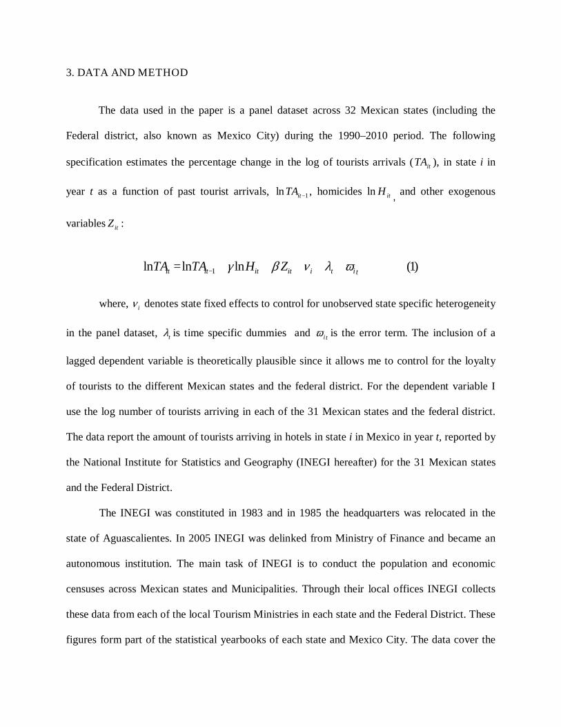
The data used in the paper is a panel dataset across 32 Mexican states (including the

Federal district, also known as Mexico City) during the 1990–2010 period. The following

specification estimates the percentage change in the log of tourists arrivals ( itTA ), in state i in

year t as a function of past tourist arrivals, 1ln −itTA , homicides ln itH, and other exogenous

variables itZ :

)1(lnlnln 1 titiitititit ZHTATA ωλνβγ +++++= −

where, iν denotes state fixed effects to control for unobserved state specific heterogeneity

in the panel dataset, tλ is time specific dummies and tiω is the error term. The inclusion of a

lagged dependent variable is theoretically plausible since it allows me to control for the loyalty

of tourists to the different Mexican states and the federal district. For the dependent variable I

use the log number of tourists arriving in each of the 31 Mexican states and the federal district.

The data report the amount of tourists arriving in hotels in state i in Mexico in year t, reported by

the National Institute for Statistics and Geography (INEGI hereafter) for the 31 Mexican states

and the Federal District.

The INEGI was constituted in 1983 and in 1985 the headquarters was relocated in the

state of Aguascalientes. In 2005 INEGI was delinked from Ministry of Finance and became an

autonomous institution. The main task of INEGI is to conduct the population and economic

censuses across Mexican states and Municipalities. Through their local offices INEGI collects

these data from each of the local Tourism Ministries in each state and the Federal District. These

figures form part of the statistical yearbooks of each state and Mexico City. The data cover the

most important tourist destinations in each state. Through its website, INEGI provides8 all the

statistical yearbooks for all states and the Federal District which contains, among several other

variables, the arrival of tourists as explained above. An advantage of these data is the fact that

the number of tourist arrivals can be separated into international and national tourist arrivals.

Unfortunately, the dataset does not provide information on the different nationalities of

international tourists nor on the states of origin of the local tourists.

I use three variables of tourist arrivals. Firstly, I look at overall arrivals of tourists. Secondly, I

separate the international tourist arrivals from the national tourist arrivals and compare the effect

that an uprise in violent crime has on both tourists categories. In order to control for violent

crime, I use the number of deaths resulting from homicides reported in state i in year t. The

rationale for this is that violent events leading to several killings attract more the attention of

local and international media. For instance, at the time of writing of this paper there has been

again a mass killing in different locations of Mexico. Soon after this event the coverage of this

notice was to be found in several newspapers across the world9.

I use two datasets on homicides. The first dataset on homicides comes from the yearly mortality

statistics gathered by INEGI10 and corresponds to the period 1990-2010. The homicides are

registered in the agency of the Public Ministry of the municipality where the crime took place.

8 See: http://www.inegi.org.mx/sistemas/productos/ for more information on the statistical yearbooks of each state and Mexico City. 9 http://www.lemonde.fr/ameriques/article/2012/05/13/mexique-37-cadavres-abandonnes-au-bord-d-une-route_1700533_3222.html http://www.bbc.co.uk/news/world-latin-america-18052540 http://www.faz.net/aktuell/gesellschaft/drogenkrieg-in-mexiko-los-zetas-enthaupten-49-menschen-11750742.html 10 For details on mortality statistics see: www.inegi.org.mx/est/contenidos/espanol/proyectos/continuas/vitales/bd/mortalidad/anexos/introduccion.asp?s=est&c=11142

This information is then delivered to the local INEGI offices across the different states and form

part of the Mortality Statistics of INEGI.

It is important to mention that for all crime data in Mexico there is the distinction to be made

between the, by INEGI, so called “register year” and “occurrence year”. The former represents

the year in which a criminal offence was registered and the latter shows the exact year in which a

criminal offence took place. It is usually the case that criminal offences are not always, for

several reasons, reported to the authorities when they happen. Thus the raw data show that there

are crimes which occurred in the past, say in 1990 but, are registered until 1998.

I only consider homicides which took place from 1990 onwards since the availability on tourism

data starts from 1990 onwards. Unlike other crime incidents data, the homicides data does not

seem to have under reporting bias as the data reported appears to be consistent across the states.

The second dataset on homicides is from an NGO11. It combines data from INEGI and BIIACS.

BIIACS12 is a databank on information for applied research in the social sciences from the

Centre for Research and Teaching in Economics, CIDE, in Mexico City. This dataset is only

available for the period 1990-2008.

Additional to the homicides variable, I also consider other forms of violent crime which

do not necessarily end up in death for the victim but are severe offences. I use data on

kidnapping, violent assault and rape and sum them up across states in order to construct a

variable which I label “Violent offences”. Contrary to the homicide data, I observe that there is

for all states a sudden increase in the number of cases recorded from the year 1996 to the year

1997 onwards. These violent crime data where downloaded from the INEGI website as well.

Despite of these crimes being severe offences, I do not expect them to have an intimidating

11 See: http://www.seguridadpublicaenmexico.org.mx/ 12 See: http://www.biiacs.cide.edu/

effect on tourist arrivals. The results of the model using these data will be presented in the

forthcoming version of this paper.

Figures 1, 2 and 3 show the number of tourist arrivals across the states during the period 1990-

2010. Figure 1 shows tourists preference for Distrito Federal, Veracruz, Jalisco and Quintana

Roo in this order. From figure 2 we can see that most International Tourists visit the following

states Quintana Roo, Distrito Federal, Baja California and Jalisco. These states are

internationally known for their beaches in the Caribbean Sea and the Pacific Ocean and are home

of several archeological parks and Mexican folklore. From figure 3, we see that national tourists

direct their preferences towards Federal District, Veracruz, Jalisco and Guerrero. Figure 4 shows

the number of homicides which took place across states during the period 1990-2010. It can be

seen that most homicides took place in following states: Estado de Mexico, Distrito Federal,

Chihuahua, Baja California, Guerrero, Michoacan, Oaxaca, and Sinaloa. It is worth to mention

that Estado de Mexico is the most populated state according to INEGI. Most of these states are

also victims of intense drug violence between the drug cartels and the state police and

paramilitary forces. (Ríos 2012) However, note that Distrito Federal, Baja California and

Guerrero are still in the preferences of tourists. Furthermore, figure 5 shows how violence is

distributed across states if we consider homicides as a rate per 100,000 inhabitants and use both

datasets. We see that in this case Chihuahua is the most violent state followed by Sinaloa and

Guerrero. This is in line with the recent work by Ríos (2012) mentioned above.

The vector of control variables (Zit) includes other potential determinants of tourist

arrivals reported in state i during year t which I obtain from the existing literature on the subject.

I follow Neumayer (2004) on the relationship between political violence and tourism demand,

and Crouch (1994) study of international tourism demand.

As consumers, tourists also decide where to go based on the price of the goods they want to

purchase; for instance holiday packages, which in some cases include flights and hotel

reservations. In order to account for the differences in prices I use the price indexes of the main

cities in each Mexican state and the Federal District. These data were computed by the Mexican

Central Bank and are used in the construction of the main national inflation index. It is important

to mention that since the summer 2011, INEGI is responsible for conducting the inflation

measurement and for reporting it to the Federal Government and to the public. However, since I

only consider the period 1990-2010, these data are taken from the Mexican Central Bank. I

would expect a negative and significant sign for this variable. Higher prices can induce tourists

to change their preferences and visit some other cheaper destination.

I use the natural logarithm of the gross domestic product per capita in state i during year t as a

proxy of economic welfare. I expect a positive and significant effect. A better economic

environment enhances appropriate conditions for the stay of tourists. These data were collected

from the National Accounts System of INEGI.

The variable urbanization is the amount of people living in urban areas as a share of total

population in state i during year t. I expect a positive and significant sign in this variable since

urban areas are known for providing a wide range of amenities for tourists for instance, health

services and public transport among others. This variable is drawn from the population census

data compiled by INEGI. Furthermore, I use the log of the number of establishments offering

overnight accommodation per capita in state i during year t to proxy for tourism infrastructure.

This variable includes hotels, hostels and guest houses. The data is originally from the Tourism

Ministry of each state, which reports on a yearly basis all tourism statistics to INEGI. These

statistics form part of the statistical yearbooks of each state provided by INEGI.

Additionally, I control for the transport infrastructure within the country when using the log of

the number of kilometers of roads available in in state i during year t. Once in the country,

tourists might be willing to visit other cities or towns near to their first destination. It is true that

some tourists would prefer to use air transportation. However, there is not much variation trough

time in the number of airports in each state. The data are from the Transportation and

Communications Ministry of each state. These statistics are as well provided to INEGI and form

part of the statistical yearbooks of each state too. I would expect a positive and significant effect

of this variable on the arrivals of tourists.

A further variable which tourists take into account for holidaying is the weather. Given the

geographic location of Mexico with a coast length of 7,828 kilometers on the Pacific Ocean side

and with a coast length of 3,249 kilometers on the side of the Gulf of Mexico and the Caribbean

Sea, the country experiences throughout a year several tropical storms which derive in hurricanes

of high intensity. Thus, I use the number of hurricanes which caused the worst floods in state i

during year t and construct a dummy variable which takes the value of one if a state was hit by a

hurricane in year t. In general, a hurricane can hit more than one state in the same year. The data

are from the Meteorological National Service13 and from the Engineering Institute of the

National Autonomous University of Mexico (UNAM)14.

3.1 Endogeneity concerns

It can potentially be the case that the number of tourists visiting a country originates more

crime. Tourists are new to the destination they visit; this lack of information puts them in a

13See: http://smn.cna.gob.mx/index.php?option=com_content&view=article&id=38&Itemid=46 14 See: http://www.iingen.unam.mx/es-mx/Paginas/default.aspx

riskier situation more easily than local people. Thus, criminals may see in them an easier prey.

This applies to both, national and international tourists.

In order to control for the direction of causality I use a dynamic model of Granger

Causality (Granger 1969). Following this model, the variable x is said to “Granger cause” a

variable y if the past values of the x help explain y, once the past influence of y has been

accounted for (Engle and Granger 1987). I stick to Dreher and Siemers (2009) to account for

Granger Causality in a panel setting as:

)2(,1

,1

titijtiitj

jtiitj

it xyy τζδϕϖρρ

++++= −=

−=

∑∑

Where, the parameters are denoted as: itϖ and itϕ for country i during the year t, the

maximum lag length is represented by ρ. While δi is unobserved individual effects, ζt is

unobserved time effects. tiτ represents the error term. Under the null hypothesis, the variable x is

assumed to not Granger cause y, while the alternative hypotheses allow for x to Granger cause y

after controlling for past influence of the variable y. Joint F-Statistics are used to gauge the joint

significance of tourist arrivals on homicides. Tables 5, 6 and 7 show evidence in favor of the null

hypothesis of no endogeneity for the three classifications of the dependent variable, namely

tourist arrivals as a total, international tourist arrivals and national tourist arrivals. These tables

also confirm my results in that the immediate past realizations of violent events do not affect

tourist arrivals. In table 7 there is only a slightly significant and negative effect in the first lag of

homicides on national tourist arrivals, which can account for the fact that national tourists might

be better informed than international tourists since the former are confronted on a more

frequently basis with the continuous violent events happening in Mexico. However, this effect

vanishes as I include more controls in the model as explained in the next section.

4. EMPIRICAL RESULTS

Table 1 presents the baseline results capturing the effect of homicides on the arrival of

overall tourists, international tourists and national tourists implementing fixed effects

estimation15. Table 2, also presents a fixed effects estimation. It addresses the question whether

tourists consider contemporaneous violent events more, rather than past violent events. In this

specification I lagged the homicides variable by one period.

According to Hsiao (1986), in a fixed effects panel model, the correlation between the

error term and the lagged dependent variable may render the estimates of the parameters bias and

inconsistent. This issue is quite serious in panel data sets with a small number of time series

observations and a large number of units. Increasing the number of units would not lead to better

estimates if the number of time series observations remains small. (Anderson and Hsiao, 1982)

In order to obtain consistent estimators, one possibility could be to implement instrumental

estimators. Nevertheless is important to note that, although GMM and IV estimators possess

good asymptotic properties, these estimators are still biases in a finite sample application,

Potrafke (2009). I follow Potrafke (2009) and use the dynamic bias corrected LS estimator

proposed by Bruno (2005a, 2005b) 16. Using asymptotic expansion techniques, Kiviet (1995,

1999) calculates approximation formulas for correcting the finite-sample bias of the least square

15 The Hausman test supports the fixed effects model specification. These results are available upon request. 16 As in Potrafke (2009), the results obtained from this method refer to the Blundell and Bond (1998) estimator as the initial one. The instruments are collapsed as suggested by Roodman (2006). I also undertake 50 repetitions of the procedure to bootstrap the estimated standard errors. The results are strong to changes in the number of repetitions such as 100, 200 and 500 and when using the Arellano and Bond (1991) estimator as the initial one.

estimator. In a further paper, Bun and Kviet (2003) redevelop Kiviet´s (1999) bias approximation

using a more austere formula. Bruno (2005a) generalizes the bias approximation formula of Bun

and Kviet (2003) and extends the analysis for unbalanced panels. The bias-correction procedure

involves some consistent estimates as a first step. The Blundell-Bond (1998) system GMM

estimator is used for these consistent estimates in this paper. Tables 3 and 4 present the bias-

corrected estimation results of the dynamic panel data model. I explain these results in the

robustness checks section. It will be seen there that my results are not affected by the potential

bias discussed above.

It is important to mention that in each table I use the two different homicide data

previously mentioned. Wherever only the homicide data from INEGI were used, I label the

corresponding columns with an “A”. On the other hand, wherever the homicide data from INEGI

& BIIACS is used, I label the corresponding columns with a “B”. Table 3 presents the results of

the Hausman test, which favour a fixed effects model specification. Table 4 presents results of

Granger causality test. From these results we see that there is no reverse causality. I discard the

possibility of tourism having an effect on homicides. The summary of data statistics is presented

in appendix 2.

Beginning with column 1 in table 1, the results show that, when using the homicide data

from INEGI and holding other factors constant, a one percentage increase in homicides

significantly leads to a roughly 15 percentage decrease in tourism at 5% level. This effect

coincides when we use the alternative data for homicides, namely those which include INEGI

and BIIACS data. In this second case, a one percentage increase in homicides leads to a roughly

19% decrease in tourism. From these results it can be seen that violent crimes are deterring

tourists in general. At this point it is interesting to ask whether this effect is similar or not for

international and national tourists. It is expected that international tourist are most deterred by

violent crime than national tourists. The latter have more information to what is happening in the

country. Thus, they have the advantage of better knowing where violence is worst and where not.

The former receive the information about crime in Mexico through the international news. When

a criminal event of high impact takes place, this is promptly communicated in the international

media. Following on this, the countries of origin of the international tourists warn their tourist

not no visit certain places in the country or better to choose completely other destination for

holidaying. Using the INEGI data, Column 3 shows the effect of violent crime/ homicides on the

arrival of international tourists. When holding other factors constant, a one percentage increase

in homicide leads to a 33% decrease on the international tourist arrivals. Furthermore, if we use

the alternative data on homicides, this effect remains in the same direction, namely a rough 32%

decrease in international tourist arrivals when homicides increase in one unit. It is interesting to

see that the effect of violent crime on international tourism is more nuanced than tourism in

general. At this point, the question whether this effect is the same or not for national tourists

comes into picture. This is done in Columns 5 with the INEGI homicide data and in Column 6

with the INEGI and BIIACS data. Column 5 shows that, holding other factors constant, the effect

of homicides on national tourist arrivals is a significant decrease of 12% at the 5% level. The

same applies when using the alternative homicide data in column 6. However, this effect is here

of the magnitude of 16% and also significant at the 5 % level. It is shown that violent crime

actually deters both types of tourists however, as expected this effect is stronger for the

international visitors.

As a next step I look at whether past crime events influence the arrival of tourists.

Tourists might cancel out their vacation if a high impact crime event takes place just before they

start their travel. Unfortunately the data on arrivals cannot be disaggregated by months. As a

result I consider the first lag of the homicide variable to control for immediate past effects of

crime on tourist arrivals. Table 2 shows the results for this specification and presents as well

estimations for tourists in general and separated by international and national tourists. Column 1

shows that a one percentage point increase in homicides leads to a decrease of tourist arrivals by

about 12%. This effect is significant at the 10 % level. The coefficient of the lagged homicide

variable, although negative, it is not significant. When using the alternative data on homicides, I

find a similar result, meaning that the contemporaneous effect of homicides on tourist arrivals is

negative and significant at the 10 % level. In this case tourist arrivals are reduced by roughly

17% and the one lagged value of the homicides variable, although negative, is insignificant.

Thus, tourists arrivals in general are not driven by past violent crime realizations but by those

violent criminal events which are contemporaneous to their vacations. As I did before, I look at

this effect after distinguishing international tourists from national tourists and using both

homicide databases.

Columns 3 and 4 show the results for the international tourist arrivals. Using the data

from INEGI, Column 3 shows that a one percentage point increase in homicides leads to a

decrease of 31% in international tourist arrivals; this is significant at the 1% level. The

coefficient of the lagged homicide variable, although negative, remains insignificant. This result

also holds when the alternative homicide data are used in Column 4. In this case, the magnitude

of the reduction in international tourist arrivals is of 31% but significant at the 5% level. Thus, it

is the contemporaneous level of homicides which intimidates international tourists and not the

past homicide events. This can be interpreted as the fact that international tourists do care about

their personal security when they are about to go on vacation and are not that interested on past

events. Here it is worth to mention that, despite the insignificance of the lagged homicide

variable, the sign remains negative. Furthermore, when looking at the national tourist arrivals in

Columns 5 and 6, it can be seen that the results are sensitive to the homicide data source. For

Column 5 the significance of the homicide variable, contemporaneous and lagged, goes away.

However, in Column 6 the homicide variable is significant at the 10% level and its first lag is not

significant. Thus, from tables 1 and 2 we can see that international tourists are most intimidated

by violent crime than national tourists. As mentioned before, this can be due to information

asymmetries arising from the location of tourists which shape the perception of tourists about

their decision for holidaying in Mexico.

Regarding the control variables, tables 1 and 2, show that prices do matter for tourism.

An increase in prices will lead tourists to choose other destinations. We see that, holding other

factors constant, a one percentage increase in inflation reduces the arrivals of tourists in general

by 6%. This effect is significant at the 10% level. This effect is similar in both tables and when

using the alternative homicide data from INEGI & BIIACS, this effect remains around 6% as

well. It is interesting to see that this effect is no more significant, although negative, for the

international tourists but only for the national tourists. Thus, prices are not an important

determinant of international tourism flows. Most of the international tourists visiting Mexico are

coming from the United States, Canada and European countries belonging to the European

Monetary Union. Due to the exchange rate advantage it is cheaper for international tourists to

holiday in Mexico than for the national tourists. This can also be seen in column 5 and 6 of tables

1 and 2. A rise in the prices matters more for national tourism than for international tourism.

Certainly, the higher the concentration of people in cities, the higher are the victimization

rates of crimes as pointed out by Gaviria and Páges (2002) in their study on Patterns of crime

victimization in Latin American cities. However, cities not only have problems but also

advantages as agglomeration of services and amenities which result attractive for tourists. It is

important to note that the correlation coefficients among the homicides variables I use and

urbanization is 0.08 and 0.04 for the INEGI and INEGI & BIIACS data respectively. Thus,

holding other factors constant, a one percentage point increase in the share of people living in

urban areas leads to a 3% increase in the arrival of tourists. This effect is significant at the 5%

level in tables 1 and 2 only for the INEGI data. Additionally, international tourists are more

attracted to urban areas than national tourist. This is consistent in both tables. Moreover, the

infrastructure for tourists, reflected in the number of establishments offering overnight services

per capita, is also important for tourism. A one percentage point increase in hotels per capita

increases the arrivals of tourists by 55%. Similarly as with urbanization, this effect is significant

at the 5% level. When looking at international and national tourists, this effect remains

significant at the 5 % only for the latter. Finally, I expect tourists past arrivals of tourists to

explain today´s arrivals. If visitors of a certain location have an enjoyable experience during their

stay, they most probably will visit the same location or country again in the future. This has also

influence on other fellow citizens when they return back to their place of residence, thus,

rumours or visit recommendations do matter for tourism markets. We see in tables 1 and 2 that

past tourist arrivals do matter for today´s arrivals. These results remain significant at the 1%

level for international, national tourists and both together. The availability of hotels variable

remains significant for tourism in general and for national tourists only. This does not necessarily

mean that such kind of infrastructure is not important for international tourists but it would rather

represent the fact that international tourists value their security more than the availability of

hotels and recreation infrastructure. Interestingly, I do not find any effects of per capita GDP,

Storms and Highways.

Before moving further towards robustness checks, I focus on the results of the model

when implementing the Dynamic Bias Corrected Estimator proposed by Bruno (2005). As table

3 shows, the results remain qualitatively unchanged in the sense that international tourists are

more intimidated by violent crime. Thus, a one percentage point increase in homicides leads to a

reduction of 33 % in the arrivals of international tourists. When using the alternative data set on

homicides, this reduction is of 32%, which is similar to the result found in table 1 for this

coefficient. The arrivals of national tourists are also negatively affected by violent crime.

Nevertheless this finding is now significant at the 10% level; previously it was significant at the

5% level as showed in table 1. This also applies when using the alternative homicide data. Thus,

violent crime reduces the arrivals of national tourists by 12% and 16% respectively.

Table 4 shows the results of implementing the model with the dynamic bias corrected

estimator and the inclusion of one lag in the homicide variable. As pointed above, this will allow

me to know whether past realizations of violent events are as important as those events taking

place in the same year when tourists are going on vacation. It is interesting to see that past

violent events do not have any significant effect for both tourist types. Only the arrivals of

international tourists remain significant and negative as in table 2 and the significance level

changes from 1% to 5%. The alternative homicide data show the same significance level as in

table 2 with fixed effects method. In both, tables 2 and 4, the magnitude of the reduction in

arrivals of international tourists is 31% after controlling for the immediate past violent events.

Coming now to the control variables, in both, tables 3 and 4, their behaviour is similar.

The variable for inflation is significant and negative in all specifications. This effect is

less significant for international tourists than for nationals. As argued above this might reflect a

higher purchasing power of international tourists, which makes them not to care about prices as

much as national tourists do. Furthermore, it seems that international tourists are more attracted

to urban areas than national tourists. This is in line with the results found in the fixed effects

specification. Contrary to the fixed effects specification, now the variable which controls for

overnight establishments is significant for both types of tourists. The remaining control variables

do not show any significance as in the fixed effects estimation.

4.1 Checks on Robustness

I examine the robustness of the main findings in the following ways. First, I exclude

those states which have more than 4 missing observations in the dependent variable. These states

are Coahuila, Estado de México, Hidalgo, Nayarit, Puebla, and Tamaulipas. The missing

observations range from 6 to 10. As an additional test for robustness, I exclude the few

observations with extreme values in tourist arrivals. Despite both robustness checks, the baseline

results are qualitatively unchanged, suggesting that the results are not driven neither by those

states with substantial missing observations nor by extreme values of the dependent variable. The

results of these robustness checks are not reported because of space considerations, but they are

replicable using the paper´s dataset and do files.

Given this evidence, I can safely argue that violent crime exerts a negative impact on

tourism in Mexico. This effect is stronger for the international tourists than for the nationals.

CONLCUSION

High criminality is nothing new in Mexico. However, during the last 4 ½ years Mexico

has experienced an increasing wave of violence as a result of competition among the DTOs for

the trafficking routes into the United States and the enforcement measures taken by the Mexican

Federal Government. These events have undoubtedly damaged the image of the country abroad

and put a serious burden on the life of citizens. However, it is important to note that this violence

is not spread all around the country. Some states have the same murder rates as European

countries. For instance, Yucatan has the same murder rate as Belgium. However, with the

advancement of technology, information is easily and quickly transmitted throughout the world.

News about violence and conflict are not the exception; on the contrary, this kind of news

change the perception people can have about municipalities, cities and countries.

This paper has investigated the effect of violent crime on the arrival of tourists in Mexico.

The point made here is that international tourists are more prone to be intimidated by the levels

of violence in Mexico. On the other hand, the national tourists are better informed about what is

going on in the country and thus better know about the riskier regions. Much has been said in the

media as to whether uprising crime in Mexico has had a negative impact or not on its tourism

industry with opinions going in both directions. Nonetheless, no paper has confronted this claim

with the data. This paper empirically analyzes the impact of crime on the arrivals of tourists in

Mexico for the period 1990 to 2010. Using a panel data set for the 31 Mexican federal states and

a federal district, I find a negative and significant effect of homicides on tourists’ arrivals.

Furthermore, when disaggregating the tourist arrival data into local and international, I find that

international tourists seem to be more intimidated from homicides than locals. These findings are

robust to alternative estimation techniques and samples.

Table 1: Tourist Arrivals, Total, International and National: Fixed Effects estimations

(1) (2) (3) (4) (5) (6)

Variables Arrivals: Total-A

Arrivals: Total-B

Arrivals: Foreign-A

Arrivals: Foreign-B

Arrivals: National-A

Arrivals: National-B

Arrivals Total- (log) t-1 0.528*** 0.489***

(0.0685) (0.0854)

Arrivals Foreign- (log) t-1 0.453*** 0.343***

(0.0882) (0.0900)

Arrivals Local- (log) t-1 0.589*** 0.577***

(0.0575) (0.0716)

Homicide (log) INEGI -0.145** -0.330*** -0.115**

(0.0581) (0.114) (0.0525)

Homicide (log) INEGI-BIIACS -0.189** -0.319** -0.161**

(0.0839) (0.142) (0.0773)

Inflation -0.0590* -0.0639* -0.0676 -0.0714 -0.0506* -0.0550*

(0.0306) (0.0325) (0.0513) (0.0537) (0.0259) (0.0274)

State per Capita GDP (log) -0.166 0.158 0.272 0.582 -0.211 0.221

(0.317) (0.464) (0.517) (0.565) (0.303) (0.460)

Urbanization 0.0260** 0.0248 0.0619** 0.0820*** 0.0260** 0.0238

(0.0116) (0.0186) (0.0249) (0.0285) (0.0113) (0.0179)

Hotels per Capita (log) 0.553** 0.629** 0.618 0.707 0.489** 0.540**

(0.222) (0.265) (0.402) (0.471) (0.193) (0.228)

Storms -0.0276 -0.00808 -0.0282 0.00508 -0.0322 -0.0116

(0.0400) (0.0420) (0.0818) (0.0986) (0.0384) (0.0410)

Roads (log) -0.000849 -0.0268 -0.137 -0.300 0.0215 0.0197

(0.0820) (0.0910) (0.218) (0.257) (0.0801) (0.0796)

Constant 12.94*** 11.60** 11.59* 10.21 10.95*** 8.676**

(4.087) (4.580) (6.587) (6.785) (3.714) (4.022)

Hausman test p > chi2 0 0 0 0 0 0

Time specific dummies YES YES YES YES YES YES

Number of States 31 31 31 31 31 31

Number of Observations 490 433 485 430 487 432

R-squared 0.553 0.509 0.340 0.287 0.615 0.575

Method Fixed Effects Fixed Effects Fixed Effects Fixed Effects Fixed Effects Fixed Effects

Notes: (a) Robust standard errors in parentheses *** p<0.01, ** p<0.05, * p<0.1

(b) Dependent Variable is Arrivals of Tourists as a total, international, and national

(c) A refers to the data solely from INEGI

(d) B refers to the data from INEGI & BIIACS

Table 2: Do Tourists forget? Tourist Arrivals, Total, International and National: Fixed Effects estimations

(1) (2) (3) (4) (5) (6)


Arrivals: Total-B

Arrivals: Foreign-A

Arrivals: Foreign-B




(0.0684) (0.0860)


(0.0870) (0.0906)


(0.0574) (0.0728)

Homicide (log) INEGI -0.118* -0.312*** -0.0763

(0.0682) (0.111) (0.0626)

Homicide (log) INEGI t-1 -0.0531 -0.0361 -0.0786

(0.0683) (0.0930) (0.0605)

Homicide (log) INEGI-BIIACS -0.165* -0.311** -0.136*

(0.0834) (0.130) (0.0798)

Homicide (log) INEGI-BIIACS t-1 -0.0543 -0.0195 -0.0563

(0.0923) (0.112) (0.0878)

Inflation -0.0604* -0.0652* -0.0686 -0.0719 -0.0526** -0.0563**

(0.0306) (0.0329) (0.0514) (0.0545) (0.0255) (0.0273)


(0.320) (0.474) (0.527) (0.573) (0.302) (0.468)

Urbanization 0.0271** 0.0252 0.0627** 0.0822*** 0.0275** 0.0242

(0.0116) (0.0189) (0.0242) (0.0284) (0.0112) (0.0181)

Hotels per Capita (log) 0.558** 0.636** 0.621 0.709 0.497** 0.548**

(0.222) (0.268) (0.404) (0.476) (0.193) (0.229)

Storms -0.0268 -0.00779 -0.0275 0.00529 -0.0307 -0.0113

(0.0403) (0.0427) (0.0816) (0.0990) (0.0391) (0.0417)

Roads (log) -0.00389 -0.0293 -0.139 -0.301 0.0164 0.0170

(0.0817) (0.0903) (0.217) (0.257) (0.0801) (0.0787)

Constant 13.23*** 11.94** 11.77* 10.31 11.38*** 9.029**

(4.118) (4.675) (6.693) (6.975) (3.713) (4.075)

Hausman test p > chi2 0 0 0 0 0 0.0003




R-squared 0.553 0.509 0.340 0.287 0.616 0.576

Method Fixed Effects Fixed Effects Fixed Effects Fixed Effects Fixed Effects Fixed Effects




(d) B refers to the data from INEGI &BIIACS

Table 3: Tourist Arrivals, Total, International and National: Dynamic bias corrected estimator

(1) (2) (3) (4) (5) (6)


Arrivals: Total-B

Arrivals: Foreign-A

Arrivals: Foreign-B




(0.0438) (0.0508)


(0.0535) (0.0481)

Arrivals Local- (log) t-1 0.680*** 0.685**

(0.0426) (0.0444)

Homicide (log) INEGI -0.146** -0.326*** -0-115*

(0.0662) (0.107) (0.0627)

Homicide (log) INEGI-BIIACS -0.188*** -0.320** -0.155*

(0.0723) (0.143) (0.0918)

Inflation -0.0587** -0.0635** -0667* -0.0704* -0.0500*** -0.0540**

(0.0245) (0.0251) (0.0377) (0.0388) (0.0179) 0.0248


(.0.361) (0.446) (0.688) (0.654) (0.380) (0.421)

Urbanization 0.0295 0.306 0.0645* 0.0855** 0.0308* 0.0327

(0.0202) (0.0226) (0.0356) (0.0433) 0.0186 (0.0223)

Hotels per Capita (log) 0.517*** 0.583*** 0.555** 0.634** 0.463*** 0.498***

(0.144) (0.140) (0.233) (0.316) (0.142) (0.134)

Storms -0.0254 -00487 -0.235 0.00777 -0.288 -0.055

(0.0576) (0.0707) (0.0818) (0.121) (0.0540) (0.0635)

Roads (log) 0.0133 -0.00489 -0.129 -0.289 0.0418 0.0540

(0.163) (0.162) (0.257) (0.320) (0.120) (0.153)

Constant




Method LSDV LSDV LSDV LSDV LSDV LSDV





Table 4: Do Tourists forget? Tourist Arrivals, Total, International and National: Dynamic bias corrected estimator

(1) (2) (3) (4) (5) (6)


Arrivals: Total-B

Arrivals: Foreign-A

Arrivals: Foreign-B




(0.0435) (0.0509)


(0.0544) (0.0485)


(0.0431) (0.0442)

Homicide (log) INEGI -0.118 -0.313** -0.0755

(0.0733) (0.124) (0.0712)

Homicide (log) INEGI t-1 -0.0540 -0.0243 -0.0790

(0.0922) (0.150) (0.0763)

Homicide (log) INEGI-BIIACS -0.163* -0.315** -0.132

(0.0853) (0.145) (0.101)

Homicide (log) INEGI-BIIACS t-1 -0.0536 -0.00981 -0.0512

(0.112) (0.172) (0.0960)

Inflation -0.0600** -0.0646*** -0.0671* -0.0705* -0.0520*** -0.0550**

(0.0242) (0.0250) (0.0380) (0.0394) (0.0177) (0.0248)


(0.360) (0.436) (0.688) (0.656) (0.375) (0.416)

Urbanization 0.0304 0.0305 0.0649* 0.0853** 0.0322* 0.0325

(0.0206) (0.0226) (0.0359) (0.0435) (0.0189) (0.0222)

Hotels per Capita (log) 0.520*** 0.589*** 0.555** 0.634** 0.470*** 0.505***

(0.142) (0.139) (0.228) (0.323) (0.143) (0.136)

Storms -0.0251 -0.00497 -0.0239 0.00760 -0.0277 -0.00562

(0.0582) (0.0719) (0.0816) (0.122) (0.0540) (0.0643)

Roads (log) 0.0124 -0.00586 -0.127 -0.287 0.0383 0.0527

(0.163) (0.161) (0.257) (0.319) (0.120) (0.153)

Constant




Method LSDV LSDV LSDV LSDV LSDV LSDV





Table 5: Causality tests Tourists Arrivals (Total) and Homicides

(1) (2) (3) (1) (2) (3)

Variables TA TA TA Variables HOM HOM HOM

Tourists Arrivals (log) (t-1) 0.566*** 0.379*** 0.591*** Homicides (log) (t-1) 0.678*** 1.263*** 1.181***

(0.0288) (0.108) (0.0953) (0.0689) (0.0793) (0.0920)

Tourists Arrivals (log) (t-2) 0.0214 0.177** Homicides (log) (t-2) 0.187*** 0.0894

(0.0830) (0.0818) (0.0641) (0.0804)

Tourists Arrivals (log) (t-3) -0.0623 Homicides (log) (t-3) 0.254**

(0.0510) (0.107)

Homicides (log) (t-1) -0.114 -0.128 -0.0301 Tourists Arrivals (log) (t-1) -0.00204 -0.00350 -0.0213

(0.0703) (0.0837) (0.0684) (0.0137) (0.0199) (0.0304)

Homicides (log) (t-2) -0.0588 -0.0185 Tourists Arrivals (log) (t-2) -0.0140 0.0401

(0.0823) (0.0850) (0.0194) (0.0416)

Homicides (log) (t-3) -0.0852 Tourists Arrivals (log) (t-3) -0.0651*

(0.0702) (0.0353)

Joint F-Statistics 2.65 1.49 0.85 Joint F-Statistics 0.02 0.47 1.52

Table 6: Causality tests Tourists Arrivals (International) and Homicides

(1) (2) (3) (1) (2) (3)



(0.0543) (0.0959) (0.0825) (0.0677) (0.0779) (0.0913)

Tourists Arrivals (log) (t-2) 0.0447 0.139 Homicides (log) (t-2) 0.189*** 0.100

(0.0941) (0.0955) (0.0629) (0.0800)

Tourists Arrivals (log) (t-3) -0.0379 Homicides (log) (t-3) 0.249**

(0.0686) (0.112)

Homicides (log) (t-1) -0.167 -0.144 -0.0516 Tourists Arrivals (log) (t-1) -0.00204 -0.00350 -0.0213

(0.111) (0.116) (0.104) (0.0137) (0.0199) (0.0304)

Homicides (log) (t-2) -0.119 -0.167 Tourists Arrivals (log) (t-2) -0.00624 0.0178

(0.102) (0.106) (0.0104) (0.0177)

Homicides (log) (t-3) 0.0375 Tourists Arrivals (log) (t-3) -0.0263

(0.122) (0.0206)


Table 7: Causality tests Tourists Arrivals (National) and Homicides

(1) (2) (3) (1) (2) (3)



(0.0296) (0.108) (0.0973) (0.0680) (0.0776) (0.0913)

Tourists Arrivals (log) (t-2) 0.0189 0.185** Homicides (log) (t-2) 0.190*** 0.0939

(0.0830) (0.0778) (0.0623) (0.0778)

Tourists Arrivals (log) (t-3) -0.091** Homicides (log) (t-3) 0.252**

(0.0428) (0.107)

Homicides (log) (t-1) -0.114 -0.149* -0.0562 Tourists Arrivals (log) (t-1) -0.00385 0.00116 -0.0245

(0.0693) (0.0771) (0.0627) (0.0135) (0.0198) (0.0313)

Homicides (log) (t-2) -0.0234 0.0202 Tourists Arrivals (log) (t-2) -0.0213 0.0405

(0.0843) (0.0786) (0.0207) (0.0460)

Homicides (log) (t-3) -0.0768 Tourists Arrivals (log) (t-3) -0.0618

(0.0714) (0.0378)


Appendix

Appendix 1: States under study

Aguascalientes Distrito Federal Morelos Sinaloa Baja California Durango Nayarit Sonora

Baja California Sur Estado de México Nuevo León Tabasco Campeche Guanajuato Oaxaca Tamaulipas

Chiapas Guerrero Puebla Tlaxcala Chihuahua Hidalgo Querétaro Veracruz

Coahuila Jalisco Quintana Roo Yucatán Colima Michoacán San Luis Potosí Zacatecas

Appendix 2: Descriptive Statistics

Variables Mean Standard Deviation Minimum Maximum Observations

Tourist Arrivals (Total) log 14.15577 1.098107 7.233455 16.31798 589

Tourist Arrivals (Total) log t-1 14.13433 1.107204 7.233455 16.31798 562

Tourist Arrivals (International) log 12.00465 1.668351 5.826 15.62604 586

Tourist Arrivals (International) log t-1 12.00123 1.675661 5.826 15.62604 559

Tourist Arrivals (National) log 13.92622 1.072491 6.952729 16.0395 588

Tourist Arrivals (National) log t-1 13.90193 1.080445 6.952729 16.02846 561

Homicides (INEGI) log 5.382426 1.150092 2.484907 8.737774 672

Homicides (INEGI) log t-1 5.355936 1.136255 2.484907 8.217709 640

Homicides (INEGI & BIIACS) log 5.386128 1.131877 2.484907 8.161375 608

Homicides (INEGI & BIIACS) log t-1 5.386128 1.131877 2.484907 8.161375 608

Inflation 11.87655 9.575491 2.617051 38.89253 630

State per Capita GDP (log) 4.146175 .513901 3.386864 6.176142 672

Urbanization 72.61502 14.94279 39.45287 99.76386 672

Hotels per Capita (log) -8.43469 .6558997 -10.28005 -6.645606 648

Storms .1622024 .368911 0 1 672

Roads (log) 8.883446 .6622945 7.247081 10.16591 651

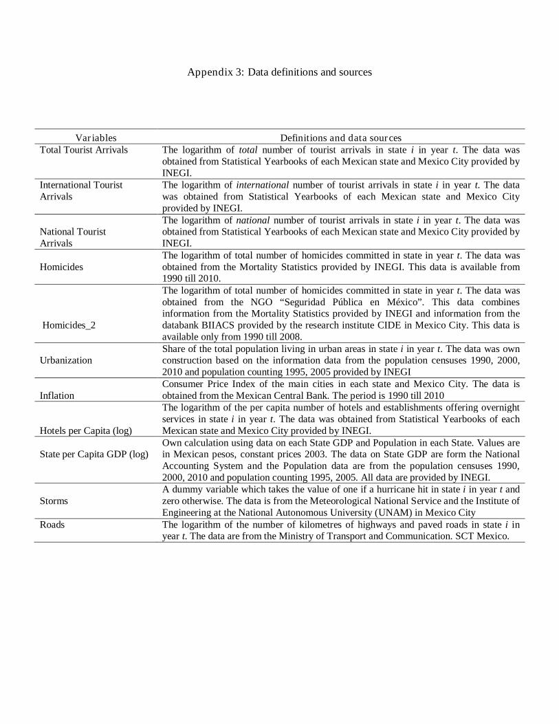
Appendix 3: Data definitions and sources

Variables Definitions and data sources Total Tourist Arrivals

The logarithm of total number of tourist arrivals in state i in year t. The data was obtained from Statistical Yearbooks of each Mexican state and Mexico City provided by INEGI.

International Tourist Arrivals

The logarithm of international number of tourist arrivals in state i in year t. The data was obtained from Statistical Yearbooks of each Mexican state and Mexico City provided by INEGI.

National Tourist Arrivals

The logarithm of national number of tourist arrivals in state i in year t. The data was obtained from Statistical Yearbooks of each Mexican state and Mexico City provided by INEGI.

Homicides

The logarithm of total number of homicides committed in state in year t. The data was obtained from the Mortality Statistics provided by INEGI. This data is available from 1990 till 2010.

Homicides_2

The logarithm of total number of homicides committed in state in year t. The data was obtained from the NGO “Seguridad Pública en México”. This data combines information from the Mortality Statistics provided by INEGI and information from the databank BIIACS provided by the research institute CIDE in Mexico City. This data is available only from 1990 till 2008.

Urbanization

Share of the total population living in urban areas in state i in year t. The data was own construction based on the information data from the population censuses 1990, 2000, 2010 and population counting 1995, 2005 provided by INEGI

Inflation Consumer Price Index of the main cities in each state and Mexico City. The data is obtained from the Mexican Central Bank. The period is 1990 till 2010

Hotels per Capita (log)

The logarithm of the per capita number of hotels and establishments offering overnight services in state i in year t. The data was obtained from Statistical Yearbooks of each Mexican state and Mexico City provided by INEGI.

State per Capita GDP (log)

Own calculation using data on each State GDP and Population in each State. Values are in Mexican pesos, constant prices 2003. The data on State GDP are form the National Accounting System and the Population data are from the population censuses 1990, 2000, 2010 and population counting 1995, 2005. All data are provided by INEGI.

Storms

A dummy variable which takes the value of one if a hurricane hit in state i in year t and zero otherwise. The data is from the Meteorological National Service and the Institute of Engineering at the National Autonomous University (UNAM) in Mexico City

Roads

The logarithm of the number of kilometres of highways and paved roads in state i in year t. The data are from the Ministry of Transport and Communication. SCT Mexico.

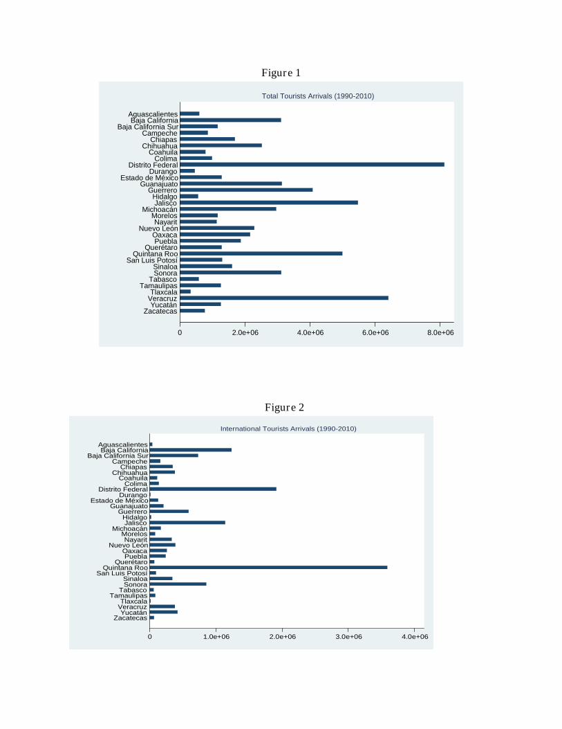
Figure 1

0 2.0e+06 4.0e+06 6.0e+06 8.0e+06

ZacatecasYucatán

VeracruzTlaxcala

TamaulipasTabasco

SonoraSinaloa

San Luis PotosíQuintana Roo

QuerétaroPuebla

OaxacaNuevo León

NayaritMorelos

MichoacánJaliscoHidalgo

GuerreroGuanajuato

Estado de MéxicoDurango

Distrito FederalColima

CoahuilaChihuahua

ChiapasCampeche

Baja California SurBaja California

Aguascalientes

Total Tourists Arrivals (1990-2010)

Figure 2

0 1.0e+06 2.0e+06 3.0e+06 4.0e+06

ZacatecasYucatán

VeracruzTlaxcala

TamaulipasTabasco

SonoraSinaloa


QuerétaroPuebla

OaxacaNuevo León

NayaritMorelos


GuerreroGuanajuato



CoahuilaChihuahua

ChiapasCampeche


Aguascalientes

International Tourists Arrivals (1990-2010)

0 2.0e+06 4.0e+06 6.0e+06

ZacatecasYucatán

VeracruzTlaxcala

TamaulipasTabasco

SonoraSinaloa


QuerétaroPuebla

OaxacaNuevo León

NayaritMorelos


GuerreroGuanajuato



CoahuilaChihuahua

ChiapasCampeche


Aguascalientes

Local Tourists Arrivals (1990-2010)

Figure 3

0 500 1,000 1,500 2,000 2,500

ZacatecasYucatán

VeracruzTlaxcala

TamaulipasTabasco

SonoraSinaloa


QuerétaroPuebla

OaxacaNuevo León

NayaritMorelos

MichoacánJalisco

HidalgoGuerrero

GuanajuatoEstado de México

DurangoDistrito Federal

ColimaCoahuila

ChihuahuaChiapas

CampecheBaja California Sur

Baja CaliforniaAguascalientes

Overview of Total Homicides

Figure 4

0 10 20 30 40

ZacatecasYucatán

VeracruzTlaxcala

TamaulipasTabasco

SonoraSinaloa


QuerétaroPuebla

OaxacaNuevo León

NayaritMorelos


GuerreroGuanajuato



CoahuilaChihuahua

ChiapasCampeche


Aguascalientes

Homicide rate per 100,000 inhabitants

INEGI INEGI-BIIACS

Figure 5

References

Anderson, T.W., and Hsiao, C. (1982), Formulation and Estimation of Dynamic Models

UsingPanel Data. Journal of Econometrics 18, 67-82

Arellano, M., and Bond, S. R. (1991), Some Specification Tests for Panel Data: Monte Carlo Evidence and an Application to Employment Equations. Review of Economic Studies 58, 277-298.

Becker, G. S. (1968), Crime and Punishment: An economic approach. Journal of Political Economy 76:169-217

Blundell, R., and Bond, S., (1998), Initial Conditions and Moment Restrictions in Dynamic Panel Data Models. Journal of Econometrics 87, 115-144

Bodea, C., and Elbadawi, I. (2008) Political Violence and Economic Growth. World Bank Policy Research Working Paper No. 4692

Braakmann, N. (2012), How do individuals deal with victimization and victimization risk?

Longitudinal evidence from Mexico. Journal of Economic Behavior & Organization forthcoming.

Bruno, G.S.F. (2005a). Approximating the bias of the LSDV estimator for dynamic unbalanced panel data models. Economics Letters, 87, 361-366

Bruno, G.S.F. (2005b). Estimation and inference in dynamic unbalanced panel data models with small number of individuals. Stata Journal, 5(4), 473-500

Bun, M.J.G. and Kiviet (2003) On the diminishing returns of higher order terms in asymptotic expansions of bias, Economics Letters 79, 145-152

Chen, S., Loayza, N., and Reynal-Querol, M. (2008) The Aftermath of Civil War. The World Bank Economic Review Vol. 22, Issue 1, 63-85

Collier, P., and Hoeffler, A. (2004) Greed and Grievance in Civil War. Oxford Economic Papers 56 (2004), 563-595

Crouch, I. G. (1994) The Study of International Tourism Demand: A Review of the Findings.

Journal of Travel Research 33:12 (12-23)

De Albuquerque, K. and McElroy J. (1999) Tourism and crime in the Caribbean. Annals of Tourism Research 26:968-84

Dell, M. (2011) Trafficking Networks and the Mexican Drug War. (Job Market Paper), Massachusetts Institute of Technology. Department of Economics.

Detotto, C. and Otranto, E. (2010) Does Crime Affect Economic Growth? Kyklos Vol.63 Issue 3, 330-345

Dreher A., and Siemers, L-H., (2009). The Nexus between Corruption and Capital Account Restrictions. Public Choice, 140(1), 245-265.

Ferreira, S. and Harmse, A. (2000) Crime and tourism in South Africa: International tourists´ perception and risk. South African Geographical Journal 82:80-85

Gaviria, A. and Pagés, C. Patterns of crime victimization in Latin American cities. Journal of Development Economics Vol. 67(2002) 181-203

Hsiao, C. (1986) Analysis of Panel Data. Cambridge: Cambridge University Press.

Kiviet, J.F. (1995) On bias, inconsistency and efficiency of various estimators in dynamic panel data models, Journal of Econometrics 68, 53-78

Kiviet, J.F. (1999) Expectation of Expansions for Estimators in a Dynamic Panel Data Model; Some Results for Weakly Exogenous Regressors. In: Hsiao, C. Lahiri, K., Lee, L. F., Pesaran, M.H. (Eds.), Analysis of Panel Data and Limited Dependent Variables. Cambridge University Press, Cambridge.

Levantis, T. and Gani, A. (2000) Tourism demand and the nuisance of crime. International Journal of Social Economics 27:959-67

Longmire S. M., and Longmire IV J. P., (2008) Redefining Terrorism: Why Mexican Drug Trafficking is More than Just Organized Crime. Journal of Strategic Security Vol. 1 (2008) 35-52

Neumayer, E. (2003) Good Policy Can Lower Violent Crime: Evidence from Cross-National Panel of Homicide Rates, 1980-97. Journal of Peace Research Vol. 40, No. 6, 619-640

Neumayer, E. (2004) The Impact of Political Violence on Tourism: Dynamic Cross-National Estimation, Journal of Conflict Resolution Vol. 48, No. 2, 259-281

Neumayer, E. and Plümper, (2011) Foreign Terror on Americans. Journal of Peace Research 48(1): 3-17

Potrafke, N. (2009) Did globalization restrict partisan politics? An empirical evaluation of social expenditures in panel of OECD countries. Public Choice 140:105-124

Ríos, V. (2012) Why did Mexico become so violent? A self-reinforcing violent equilibrium caused by competition and enforcement. Department of Government, Harvard University. Forthcoming in 2013 in Trends in Organized Crime

Roodman, D. (2006) How to Do xtabond2: An Introduction to “Difference” and “System” GMM in stata- Working Paper 103 Center for Global Development. Working Paper 103.

Texeira, M. (1995) O colapso do turismo e a violência no Brasil. Conjuntura Econômica 49:63-63

Texeira, M. (1997) A violência está matando o turismo no Brasil. Conjuntura Econômica 51:32-34

nicolás corona juárez please do not cite without … · 2012-06-11 · mexico3.other scholars...

Documents