news arrival, jump dynamics, and volatility …the journal of finance •vol. lix, no. 2 april 2004...
TRANSCRIPT
THE JOURNAL OF FINANCE • VOL. LIX, NO. 2 • APRIL 2004
News Arrival, Jump Dynamics, and VolatilityComponents for Individual Stock Returns
JOHN M. MAHEU and THOMAS H. MCCURDY∗
ABSTRACT
This paper models components of the return distribution, which are assumed to bedirected by a latent news process. The conditional variance of returns is a combinationof jumps and smoothly changing components. A heterogeneous Poisson process with atime-varying conditional intensity parameter governs the likelihood of jumps. Unliketypical jump models with stochastic volatility, previous realizations of both jump andnormal innovations can feed back asymmetrically into expected volatility. This modelimproves forecasts of volatility, particularly after large changes in stock returns. Weprovide empirical evidence of the impact and feedback effects of jump versus normalreturn innovations, leverage effects, and the time-series dynamics of jump clustering.
THERE IS A WIDE-SPREAD PERCEPTION in the financial press that volatility of assetreturns has been changing.
The new economy is introducing more uncertainty. Indeed, it can be arguedthat volatility is being transferred from the economy at large into thefinancial markets, which bear the necessary adjustment shocks.1
Given the impact of changes in volatility dynamics on many important finan-cial and economic decisions (such as portfolio rebalancing, derivative pricing,risk measurement, and risk management), it is important to assess the empiri-cal validity of this perception and to investigate the sources and characteristicsof changing volatility dynamics.
Volatility2 and risk can be linked to the quantity and quality of informationpertaining to a stock’s expected future earnings and cash flows. For example,
∗Maheu is from the Department of Economics, University of Toronto, and McCurdy is from theJoseph L. Rotman School of Management, University of Toronto, and is an Associated Fellow ofCIRANO. We are grateful to the editor (Rick Green) and an anonymous referee for very helpfulcomments. We also thank Toby Daglish, J.C. Duan, Robert Elliot, Adlai Fisher, and Nour Meddahi,as well as participants at the Modeling, Estimating and Forecasting Volatility Conference (Uni-versity of Montreal), the Financial Mathematics Seminar (Fields Institute), the North AmericanSummer Meeting of the Econometric Society (Los Angeles), the Northern Finance Association 2002Meetings, the Canadian Econometrics Study Group, the Waterloo Financial Econometrics Confer-ence, and workshops at Queen’s University and the University of Toronto. We also thank the SocialSciences and Humanities Research Council of Canada for financial support. Any errors are ourown.
1 “Coping with the market’s mood swings,” Financial Times, London, September 27, 2000.2 In this paper we use the term volatility to refer generically to information on the second moment
of returns.
755
756 The Journal of Finance
information that results in a resolution of uncertainty about a firm’s futureprospects can result in a large revision in current prices. According to thisview, the most important process affecting price movements is the news arrivalprocess. In Ross (1989) and Andersen (1996), the volatility of stock price changesis directly related to the rate of flow of information to the market.
For individual securities, news about anticipated cash flows and the appro-priate discount rate are particularly relevant. A noteworthy contribution inthis vein is a recent study by Campbell et al. (2001) who report that firm-levelvariance has more than doubled between 1962 and 1997, whereas market andindustry variances have remained fairly stable over that period.3 They analyzethe dynamics of idiosyncratic, industry, and market components of the volatilityof individual stock returns. We study the distributional components, in partic-ular, large versus small changes of stock returns, and how these componentscontribute to the dynamics of volatility and higher-order moments of returns.
In this paper we do not model the latent news process directly, but ratherpropose a model of the conditional variance of returns implied by the impact ofdifferent types of news. We interpret the innovation to returns, which is directlymeasurable from price data, as the news impact from latent news innovations.The latent news process is postulated to have two separate components, normalnews and unusual news events, which have different impacts on returns and ex-pected volatility for individual stocks.4 Normal news innovations are assumedto cause smoothly evolving changes in the conditional variance of returns. Thesecond component of the latent news process causes infrequent large moves inreturns. The impacts of these unusual news events are labeled jumps. There-fore, the news process induces two components in returns, which are identifiedby their volatility dynamics and higher-order moments. We model these com-ponents as normal innovations, and abnormal or jump innovations.
A potential source of jump innovations to returns can be important newsevents, such as earnings surprises. For example, in January 2000, Intel Cor-poration announced earnings that were 8.83 percent higher than the mean In-stitutional Brokers’ Estimate System (IBES) forecast. This earnings surpriseresulted in a 12.4 percent increase in price on January 14, 2000. In October2000, IBM’s negative earnings surprise of −0.18 percent led to a price changeof −16.9 percent on October 18, 2000. On November 13, 2000, an earningssurprise of −19.76 percent for Hewlett-Packard resulted in a price change of−13.67 percent. These news surprises concerning expected future cash flowsresulted in price changes well above normal and might be better captured byjumps rather than Brownian motion or normal innovations. On the other hand,less extreme movements in price (modeled as normal innovations) can be due
3 Although systematic market risk is an important part of many financial decisions, Campbellet al. (2001) emphasize that the total volatility of a firm’s return is also relevant (for arbitrageurs,for derivative pricing, for hedge funds, etc.).
4 Clark (1973) and Tauchen and Pitts (1983) use information flows to motivate price movementsand trading activity. Andersen (1996) concludes that “it is natural to hypothesize that there aretwo or more types of information arrival processes that have different implications for volume andreturn volatility persistence.”
Individual Stock Returns 757
to typical news events, as well as liquidity trading and strategic trading asinformation disseminates.5
To augment Brownian motion in an attempt to better capture the empiricaldistribution of returns, Press (1967) introduced a jump-diffusion model thatassumes information arrivals are independently and identically distributed asa Poisson process. Over an interval (t − 1, t), a random number of news eventsarrive. In this compound events model, the Poisson distribution directs thenumber of jump events occurring in the fixed interval. The expected numberof events per interval is defined as the intensity (jump frequency) of the Pois-son process. Associated with each of these news events is a jump size that isassumed to be stochastic. This basic jump-diffusion model and its many exten-sions can be applied to the effect of news flows on price changes. Of particu-lar relevance to our application are those that also incorporate autoregressivestochastic volatility (SV).
Traditional SV-jump-diffusion specifications assume a temporally indepen-dent arrival rate of jump events. There is evidence that, like the informationprocess itself, jumps tend to be clustered together. Not only do we observe sus-tained episodes of extreme volatility (for example, the SE Asian currency crisis),but even market crashes can be realized in a series of jumps over a short periodof time. Allowing for time variation and clustering in the process governingjumps may be important. For example, Bates (1991) finds systematic behaviorin the expected number of jumps around the 1987 crash using options data.Recent examples of SV-jump-diffusion specifications with time-varying jumpintensities include Andersen, Benzoni, and Lund (2002), Bates (2000), Chernovet al. (2003), and Pan (2002).6 Eraker, Johannes, and Polson (2003) allow forjumps in both returns and volatility.
We explore dependence in the arrival process governing jump events in adiscrete-time setting and extend the work of Jorion (1988) and Vlaar and Palm(1993), among others.7 Bates and Craine (1999) allow a volatility factor to drivethe intensity. Bekaert and Gray (1998), Das (2002), and Neely (1999) allow fi-nancial and macroeconomic variables to affect the jump intensity. Johannes,Kumar, and Polson (1999) consider a state dependent jump model that al-lows past jumps and observables to affect the jump probability. We develop amixed GARCH-jump model incorporating the autoregressive conditional jumpintensity parameterization proposed by Chan and Maheu (2002). Maintainingdistributional assumptions at the relevant discrete-time frequency allows usto use maximum likelihood estimation and the associated filter to infer the
5 Glosten and Milgrom (1985) and Andersen (1996) develop a market microstructure model inwhich asymmetric information and liquidity requirements induce trades in response to informationarrivals. They outline how a news event that causes a large price change can be associated withquite different volatility effects than one with less information content. Bates (2001) provides atheoretical model in which investor heterogeneity affects the impact of news events on asset prices.
6 Yu (2003) has proposed a pure jump diffusion with a time-varying intensity.7 For example, Baillie and Han (2001), Pan (1997), Nieuwland, Vershchoor, and Wolff (1994),
Feinstone (1987), and Ball and Torous (1983). Oomen (2002) discusses various extensions includinga multiple component compound Poisson model for high and low frequency jumps.
758 The Journal of Finance
distribution of the unobservable jumps. The conditional intensity process al-lows the expected arrival rate of jumps to vary over time and allows jumps tocluster. The time variation in the conditional intensity implies all high-orderconditional moments of returns are time varying. Similar to a Peso problem,jumps need not occur to have important effects on the conditional higher-ordermoments.
Linked to a particular jump event is the news impact that the jump has onprice changes. Depending on the type and the importance of the informationrevealed by the news, the stochastic jump size may be negative, positive, big, orsmall. For example, jumps can reflect good or bad news events and affect theconditional and unconditional skewness of the return distribution through themagnitude and the sign of the mean of the jump size distribution.
Therefore, the dynamics of volatility are affected by a time-varying rate ofjump arrival, stochastic jump size, and volatility clustering. The conditionalvariance in our model is a combination of a smoothly evolving continuous-stateGARCH component and a discrete jump component. In addition, unlike conven-tional parameterizations of SV-jump-diffusions, previous realizations of bothnormal and jump innovations affect expected volatility through the GARCHcomponent of the conditional variance.8 This feedback can be important becauseonce return innovations are realized, there may be strategic trading related tothe propagation of the news, liquidity trading, etc. These activities are furthersources of volatility clustering—in addition to clustering of jump arrivals.
We allow for several asymmetric responses to past return innovations. Firstly,the news impact resulting in jump innovations can have a different feedbackon expected volatility than the news impact associated with normal innova-tions. For instance, important news innovations that result in a jump maybe quickly incorporated into current prices and have a smaller effect on ex-pected volatility; or the reverse, news that results in jumps may cause fu-ture volatility. Secondly, we allow for asymmetric responses to good versusbad news in the GARCH component of volatility.9 A further flexibility is thatthe asymmetric effect of good versus bad news can be different for jump ver-sus normal innovations. These novel features allow a richer characterizationof volatility dynamics, particularly with respect to events in the tail of thedistribution.
We initially apply our model to equity returns from 11 U.S. stocks. To showthat jumps may be associated with significant news innovations, we have com-puted the probability of jumps (inferred from our model) around days that
8 GARCH specifications allow past (squared) return innovations to feedback into expected volatil-ity. Engle and Ng (1993) interpret the return innovation as the impact of news events. Their newsimpact curve summarizes the possibly asymmetric impact of good and bad news on the conditionalvariance of next period’s return.
9 Asymmetric GARCH models include Engle and Ng (1993), Glosten, Jagannathan, and Runkle(1993), and the Nelson (1991) EGARCH specification. The empirical stylized fact that negativereturn (bad news) innovations are associated with increases in volatility has become known as theleverage effect. Cho and Engle (1999) and Campbell and Hentschel (1992) provide an economicinterpretation of news effects through asymmetric volatility and its effect on the required rate ofreturn from stocks.
Individual Stock Returns 759
earnings surprises were announced. We find empirical support for our con-jecture that large innovations to returns are associated with significant newsevents. For the examples discussed above, the ex post probability of a jump forIntel is 0.94 (January 14, 2000), IBM 0.99 (October 18, 2000), and Hewlett-Packard 0.74 (November 13, 2000).
Consistent with previous studies, we find that the unconditional jump in-tensity is low. However, since the conditional jump intensity is autoregressive,jumps are likely to cluster. Therefore, IBM may have three jumps within a weekbut no jumps for the next three months. On average, jumps account for about25 percent of daily volatility. Yet, when jumps occur, their proportion of theconditional variance can shoot up to 90 percent.
Statistical tests strongly reject a constant intensity version of the model infavor of autocorrelation in the jump intensity. This time variation is very im-portant in capturing return dynamics. For example, by correctly predicting thejumps following the 1987 crash, the model’s predictions of IBM daily volatilityclosely match the quick return of realized volatility to normal levels. In contrast,we show that a benchmark asymmetric GARCH model, with t-distributed in-novations but no jumps, takes a significant period of time to return to normallevels of volatility.
Jumps affect forecasts of future volatility directly through the time-varyingPoisson arrival process. In addition, the effect of jumps on the conditional vari-ance through GARCH feedback effects is also statistically significant. However,jump innovations tend to have a smaller feedback coefficient than normal inno-vations. This evidence is consistent with the stylized fact10 that the persistenceeffect on expected volatility from large shocks to returns is often smaller thannormal innovations. Although we find the traditional good and bad news asym-metry associated with the GARCH volatility component, this appears to operatemostly when no jumps occur. In contrast, in the presence of jumps, the newsimpact curve displays less asymmetry.
It is interesting to note that the effects of jumps appear to be different fornew versus traditional economy stocks. To investigate further, we apply ourmodel to three indices of different types of firms: the DJIA, the Nasdaq 100,and the CBOE Technology index (TXX). The more volatile indices have morefrequent jumps, and these jumps have a larger impact on the return distribu-tion. All indices display significant jump clustering. This result is consistentwith evidence reported in Johannes et al. (1999).
The jump size mean is significantly negative for all three indices. This im-plies a negative conditional correlation between jump innovations and squaredreturn innovations. In other words, large negative return realizations are asso-ciated with an immediate increase in the variance. We call this a contempora-neous leverage effect. Note that this leverage effect is time varying due to thetime-varying correlation. This result of a significant contemporaneous asym-metry is associated with a somewhat weaker asymmetry between the sign oflagged innovations and the GARCH variance component. For our samples of
10 For example, Schwert (1990) and Engle and Mustafa (1992).
760 The Journal of Finance
indices, a contemporaneous leverage effect, which is captured directly by jumpsis more important than the lagged leverage effect, which is captured by theGARCH feedback structure. These results extend the evidence obtained fromtraditional GARCH models.
The structure of our model is such that the mixture of components can adaptflexibly to capture different features of the conditional distribution of returns.However, introducing more parameters involves the danger of over fitting insample. Therefore, it is important to determine whether or not the improvedin-sample fit is useful for forecasting out of sample. Using a range-based mea-sure for ex post or realized volatility, we demonstrate that for 10 of 11 firmsour model has superior out-of-sample forecasts relative to a benchmark asym-metric GARCH model with fat-tailed innovations. In addition, we provide ev-idence of superior out-of-sample forecasts for high volatility periods and forconditional forecasts following large negative moves in the market. The lat-ter two tests are designed to evaluate the dynamics in the tails of the returndistribution.
In summary, our paper provides evidence of time dependence in jump inten-sities for both individual stocks and indices using an autoregressive conditionaljump intensity parameterization; allows both normal and jump innovations tofeed back into expected volatility; and provides new results on asymmetric ef-fects of return innovations on volatility. Conditional skewness and kurtosis arefunctions of both volatility components. The conditional skewness result can beinterpreted as a time-varying contemporaneous leverage effect. This is modeledjointly with the possibility of lagged leverage effects through the GARCH feed-back structure. These novel features allow the model to perform better aroundcrash periods and other events in the tail of the distribution. With regard tothe indices studied in this paper, we document several differences betweenvolatility components associated with “old” versus “new economy” stocks. Fi-nally, our model provides superior out-of-sample conditional variance forecastsrelative to a popular benchmark model, even when the latter is allowed to havefat-tailed innovations. These superior out-of-sample forecasts should result inimprovements in financial management.
This paper is organized as follows. Section I gives a detailed account of thetwo stochastic components affecting returns, construction of the likelihood, andconditional moments. The data used in this study is presented in Section II. Adiscussion of the empirical results is presented in Section III, out-of-sampleforecasts are evaluated in Section IV, while Section V summarizes the results.An Appendix contains some theoretical calculations for the model.
I. A GARCH-Jump Model for Returns
In this section, we present a mixed GARCH-jump model for individual se-curity returns. In our model of return volatility, we maintain an unobservednews process that directs movements in prices. News events, together with in-vestors’ expectations of these events, may result in price changes. In this paper,we do not model the latent news process directly but rather propose a model
Individual Stock Returns 761
of the conditional variance of returns implied by the impact of different typesof news. We label the innovation to returns, which is directly measurable fromprice data, as the news impact from latent news innovations.
The latent news process is postulated to have two separate components, nor-mal and unusual news events. These news innovations are identified throughtheir impact on return volatility. In particular, the impact of unobservable nor-mal news innovations is assumed to be captured by the return innovationcomponent, ε1,t. This component of the news process causes smoothly evolvingchanges in the conditional variance of returns. The second component of thelatent news process causes infrequent large moves in returns, ε2,t. The impactsof these unusual news events are labeled jumps.
We begin by specifying the components of returns. Given an information setat time t − 1, which consists of the history of returns �t−1 = {rt−1, . . . , r1}, thetwo stochastic innovations, ε1,t and ε2,t, drive returns,
rt = µ + ε1,t + ε2,t . (1)
In particular, ε1,t is a mean-zero innovation (E[ε1,t | �t−1] = 0) with a Normalstochastic forcing process,
ε1,t = σt zt , zt ∼ NID(0, 1), (2)
ε2,t is a jump innovation specified so that it is also conditionally mean zero(E[ε2,t | �t−1] = 0), and ε1,t is contemporaneously independent of ε2,t.
The subsections that follow describe our parameterization of these twostochastic components of returns. In particular, we begin by specifying the pro-cess governing jumps and the distribution of jump sizes. Then we describe insome detail the components of time-varying volatility. These parametric as-sumptions allow us to optimally infer when jumps arrive through the use ofBayes rule. The next subsections summarize the conditional moments of re-turns and the construction of the log likelihood and the filter. Henceforth, werefer to the mixed GARCH-jump model with autoregressive jump intensity asGARJI.
A. Autoregressive Conditional Jump Intensity (ARJI)
Unlike the previously cited GARCH-jump mixture models, we explicitly in-corporate an autoregressive conditional intensity that governs the likelihood ofjumps occurring between time t − 1 and t. The distribution of jumps is assumedto be Poisson with a time-varying conditional intensity parameter. In partic-ular, a Poisson distribution with parameter λt conditional on �t−1 is assumedto describe the arrival of a discrete-valued number of jumps, nt ∈ {0, 1, 2, . . .},over the interval (t − 1, t). The conditional density of nt is
P (nt = j | �t−1) = exp(−λt)λjt
j !, j = 0, 1, 2, . . . . (3)
762 The Journal of Finance
The conditional jump intensity, λt ≡ E[nt | �t−1], is the expected number ofjumps conditional on the information set �t−1 . The dynamics governing λtare parameterized as
λt = λ0 + ρλt−1 + γ ξt−1, (4)
defined as an autoregressive conditional jump intensity (ARJI) model in Chanand Maheu (2002). In this model, the conditional jump intensity λt is assumed tobe autoregressive and related to last period’s conditional intensity as well as toan intensity residual ξt−1. It seems likely that the probability of jumps will varyover time, and may be sensitive to economic conditions, such as the businesscycle, bull and bear markets, and monetary policy. The specification in equa-tion (4) is a time-series approach to studying the arrival process of jumps.11
A natural measure of the persistence of this process is ρ. The restrictionsρ = γ = 0 yield a constant jump intensity as in Jorion (1988).
The jump intensity residual is defined as
ξt−1 ≡ E[nt−1 | �t−1] − λt−1
=∞∑
j=0
j P (nt−1 = j | �t−1) − λt−1. (5)
P(nt−1 = j | �t−1) is called the filter and is the ex post inference on nt−1 given timet − 1 information. More details on the filter and construction of the log likelihoodare detailed in a subsection below. E[nt−1 | �t−1] is our ex post assessment of theexpected number of jumps that occurred from t − 2 to t − 1, while λt−1 is by defi-nition the conditional expectation of nt−1 given the information set �t−2. There-fore, ξt−1 represents the change in the econometrician’s conditional forecastof nt−1 as the information set is updated (ξt−1 = E[nt−1 | �t−1] − E[nt−1 | �t−2]).Note from this definition that ξt is a martingale difference sequence with respectto �t−1,
E[ξt | �t−1] = 0 (6)
and therefore E[ξt] = 0 and Cov(ξt, ξt−i) = 0, i > 0. Hence, the intensity residu-als in a well specified model should display no autocorrelation.
There are several important features of this conditional intensity model.First, if the ARJI specification is stationary, (|ρ| < 1), then the unconditionaljump intensity is equal to
E[λt] = λ0
1 − ρ. (7)
Second, forecasts of λt+i, and therefore the conditional variance of ε2,t+i, arestraightforward to calculate. For example, multiperiod forecasts of the expectednumber of future jumps are
11 An alternative model of the conditional intensity would be a structural model in which eco-nomic variables affect the jump likelihood.
Individual Stock Returns 763
E[λt+i | �t−1] ={
λt i = 0
λ0(1 + ρ + · · · + ρi−1) + ρiλt i ≥ 1(8)
Notice that the ARJI model can be re-expressed as
λt = λ0 + (ρ − γ )λt−1 + γ E[nt−1 | �t−1]. (9)
A sufficient condition for λt > 0, for all t > 1, is λ0 > 0, ρ ≥ γ , and γ ≥ 0.12
To estimate the ARJI model, startup values of λt, ξt, t = 1 must be set. We setstartup values of the jump intensity to the unconditional value in equation (7),and ξ1 = 0.
B. The Jump Innovation and Jump-Size Distribution
The jump size Yt,k is assumed to be independently drawn from a Normaldistribution. The jump-size distribution is
Yt,k ∼ NID(θ , δ2), (10)
and the jump component affecting returns from t − 1 to t (period t) is
Jt =nt∑
k=1
Yt,k . (11)
Therefore, the jump innovation associated with period t is expressed as
ε2,t = Jt − E[Jt | �t−1] =nt∑
k=1
Yt,k − θλt , (12)
which is the sum of the stochastic nt jumps, which arrived over the time interval(t − 1, t) adjusted by E[Jt | �t−1] = θλt, so that ε2,t is conditionally mean zero.
C. Time-Varying Volatility Components
The conditional variance of returns is decomposed into two separate com-ponents: a smoothly evolving conditional variance component related to thediffusion of past news impacts and the conditional variance component associ-ated with the heterogeneous information arrival process that generates jumps.The conditional variance of returns is
Var(rt | �t−1) = Var(ε1,t | �t−1) + Var(ε2,t | �t−1). (13)
12 Note that if ρ < γ , additional restrictions on the model may be available to ensure λt > 0 forall t.
764 The Journal of Finance
The first component of the conditional variance, σ 2t ≡ Var(ε1,t | �t−1), is param-
eterized as a GARCH function of past return innovations,
σ 2t = ω + g (�, �t−1)ε2
t−1 + βσ 2t−1, (14)
where g(·) is a function of the parameter vector �, and the information set, and
εt−1 = ε1,t−1 + ε2,t−1, (15)
is the total return innovation observable at time t − 1. We label g(·) the feedbackcoefficient from past return innovations. The GARCH volatility component al-lows past shocks affecting returns to affect expected volatility, and captures thesmooth autoregressive changes in the conditional variance that are predictablebased on past news impacts.
Following Engle and Ng (1993), we associate good news with a positive im-pact on returns, (εt−1 > 0), and bad news with a negative impact on returns,(εt−1 < 0). The g(·) function detailed below allows for asymmetric effects withrespect to the impact of past good and bad news and also with respect to feed-back effects from past jump versus normal innovations.
Ideally, we want each component of εt−1 to affect future expected volatilitydifferently.13 However, we cannot perfectly separate these two stochastic com-ponents based on observed returns.14 Instead, our GARCH specification allowsthe feedback from εt−1 to flexibly respond to the composition of εt−1 through theparameter function g(�, �t−1). Volatility may be sensitive to good news versusbad news effects or whether a jump occurred last period. For instance, impor-tant news events that result in a jump may be quickly incorporated into currentprices and have a smaller effect on future volatility; or the reverse, news thatcauses jumps may cause future volatility.15 To investigate this hypothesis, weestimate the number of jumps that occurred during period t − 1 and allow it todirectly affect the feedback that εt−1 has on the GARCH variance process. Weallow for all of these responses using the following parameterization:16
g (�, �t−1) = exp(α + α j E[nt−1 | �t−1] + I (εt−1)(αa + αa, j E[nt−1 | �t−1])), (16)
where the model parameters are collected in the vector � = {α, αj, αa, αa, j},I(εt−1) is an indicator function that takes the value 1 when εt−1 < 0, and 0
13 Note that measurable shocks to the conditional intensity do propagate and affect future jumpprobability (and therefore expected volatility) separately from the GARCH specification.
14 We can calculate E[ε2,t−1 | �t−1], but this is likely to seriously understate the variability fromthe realized ε2,t−1.
15 Important news events may cause future volatility as investors absorb the importance of thenews and its effect on future cash flows and the profitability of the firm. Often important newsevents stay in the headlines for several days forcing investors to re-evaluate their expectations.
16 Along with non-negative constraints on ω and β, the exponential function ensures that theconditional variance is positive.
Individual Stock Returns 765
otherwise, and E[nt−1 | �t−1] is an ex post assessment of the expected numberof jumps that occurred between t − 2 and t − 1, using t − 1 information.
Firstly, this parameterization of σ 2t allows asymmetric responses to bad ver-
sus good news. In particular, observed negative innovations to returns (badnews) are allowed to have a different feedback on σ 2
t through the extra contri-bution of the parameters αa and αa, j.
Recall that the GARCH parameterization includes the effects of both pastnormal innovations and past jump innovations to returns, as indicated byequation (15). Our parameterization allows for a difference in the propagation ofprevious news effects that result in jumps (ε2,t−1) versus news events that causenormal innovations (ε1,t−1). Therefore, the parameter αj, scaled by the most re-cently inferred number of jumps, allows the feedback on σ 2
t from news eventscausing jumps to be different than the feedback associated with normal newsevents. In addition, we allow the news feedback on σ 2
t from the inferred numberof jumps to be different when the past news was good or bad. To illustrate: if lastperiod’s news was good and no jumps occurred, the feedback coefficient to σ 2
t isg(�, �t−1) = exp(α), while if news was good and one jump occurred, the coeffi-cient is g(·) = exp(α + αj); if last periods news was bad and no jump occurred,the feedback coefficient to σ 2
t is g(·) = exp(α + αa); and finally, if the news wasbad and was associated with one jump it is g(·) = exp(α + αa + αj + αa, j).
Given our development of the conditional jump intensity and the jump-sizedistribution, the conditional variance component associated with the jumpinnovation is
Var(ε2,t | �t−1) = (θ2 + δ2)λt . (17)
This contribution to the conditional variance from jumps will vary over time asthe conditional intensity λt varies. In other words, this component can rangefrom being small to large as the expected number of jumps changes throughtime.
One interpretation of the decomposition of the conditional variance into thetwo components is that the GARCH component σ 2
t captures the normal time-variation of volatility associated with the predictable decay of the impact, onexpected volatility, from past news innovations to returns. We interpret thistime-series effect to be related to the dissemination and diffusion of informa-tion, liquidity trading, etc. In contrast to the GARCH specification of volatility,jumps occur when a significant news event arrives that causes an unusualabrupt change in returns. For instance, a jump is likely to have occurred whenan extreme tail realization occurs in the returns process. Statistically, jumps areidentified by observations that are inconsistent with the first stochastic compo-nent of returns, ε1,t. In this case, the GARCH volatility component is unable toaccommodate the abrupt change in volatility and such observations are identi-fied as a jump. Modeling jumps and their arrival process may be a particularlyimportant feature for capturing events that lead to episodes of high volatilityas well as for incorporating higher-order conditional moment dynamics such astime-varying skewness, and kurtosis of stock returns.
766 The Journal of Finance
D. Moments of Returns
The first four conditional moments of returns for our model are
E[rt | �t−1] = µ (18)
Var(rt | �t−1) = σ 2t + (θ2 + δ2)λt (19)
Sk(rt | �t−1) = λt(θ3 + 3θδ2)(σ 2
t + λtδ2 + λtθ2)3/2
(20)
Ku(rt | �t−1) = 3 + λt(θ4 + 6θ2δ2 + 3δ4)(σ 2
t + λtδ2 + λtθ2)2
, (21)
in which Sk(rt | �t−1) is the conditional skewness of returns, and Ku(rt | �t−1) isthe conditional kurtosis. The derivation of these moments can be found in Dasand Sundaram (1997). The sign of conditional skewness depends on the signof the jump size mean, θ . With jumps in the model, all high-order conditionalmoments are effected by the conditional jump intensity λt and σ 2
t .17
In general, the g(·) function in the GARCH specification does not permit aclosed form solution for the unconditional variance. However, the unconditionalvariance of returns can be calculated for the special case of αj = αa = αa, j = 0,18
Var(rt) = ω
(1 − α − β)+ α(θ2 + δ2)
(1 − α − β)λ0
(1 − ρ)+ (θ2 + δ2)
λ0
(1 − ρ). (22)
The first term in (22) is the usual unconditional variance from a GARCH(1,1)model, the last term is the unconditional variance from the jump innovationε2,t, and the middle term is the result of the interaction of the total news impactεt−1 = ε1,t−1 + ε2,t−1 entering in the GARCH function. Details on this calculationcan be found in the Appendix.
E. Likelihood Function
Construction of the likelihood function follows. Conditional on j jumps occur-ring the conditional density of returns is Normal,
f (rt | nt = j , �t−1) = 1√2π
(σ 2
t + j δ2) exp
(− (rt − µ + θλt − θ j )2
2(σ 2
t + j δ2)
).
17 Alternative parametric approaches to modeling time-varying higher-order conditional mo-ments include Hansen (1994), Premaratne and Bera (2001), Perez, Quiros, and Timmermann(2001), and Harvey and Siddique (1999).
18 Here the GARCH is parameterized as σ2t = ω + αε2
t−1 + βσ2t−1.
Individual Stock Returns 767
Integrating out the number of jumps gives the conditional density in terms ofobservables,
f (rt | �t−1) =∞∑
j=0
f (rt | nt = j , �t−1)P (nt = j | �t−1). (23)
The filter is then constructed as
P (nt = j | �t) = f (rt | nt = j , �t−1)P (nt = j | �t−1)f (rt | �t−1)
j = 0, 1, 2, . . . , (24)
and provides an ex post distribution for the number of jumps, nt. The filter isalso applicable and useful in studying jump dynamics in simpler jump specifi-cations such as Jorion (1988). One method to assess if a jump occurred wouldbe to use the filter to find the probability that at least one jump occurred.This is, P(nt ≥ 1 | �t) = 1 − P(nt = 0 | �t), which is directly available from modelestimation.
Finally, it should be noted that these terms in the likelihood and filter involvean infinite summation. To make estimation feasible, we truncated this summa-tion at 25. In practice, for our model estimates, we found that the conditionalPoisson distribution had zero probability in the tail for values of nt ≥ 10.
II. Data
Due to the infrequent nature of jumps and our desire to obtain accurateestimates of the jump dynamics, we focused on firms with medium to longspans of available data. Daily price data for the randomly chosen firms thatfit this criteria were obtained from the Center for Research in Security Prices(CRSP) database with samples ending on December 29, 2000. These firms (startdates) are: Amgen (June 2, 1983); Apple (December 15, 1980); Coca Cola orKO (July 3, 1962); General Motors or GM (July 3, 1962); Home Depot or HD(January 3, 1983); Hewlett-Packard or HWP (July 3, 1962); Intel (January 4,1982); Johnson & Johnson or J&J (July 3, 1962); Motorola or MOT (July 3, 1962);and Texaco (July 3, 1962). In order to evaluate out-of-sample forecasts, a range-based estimate of realized or ex post volatility was constructed from intradayhigh and low price data obtained from Commodity Systems, Incorporated. Sincethis range-based measure was also used to evaluate IBM forecasts around the1987 crash, we obtained the IBM data from the same source for the periodJuly 3, 1962 to March 1, 2001. Finally, three indices were studied with samplesto the end of 2001. These indices (start dates) are the Dow Jones IndustrialAverage or DJIA (January 4, 1960); Nasdaq 100 (February 1, 1985); and theCBOE Technology Index or TXX (May 16, 1995).
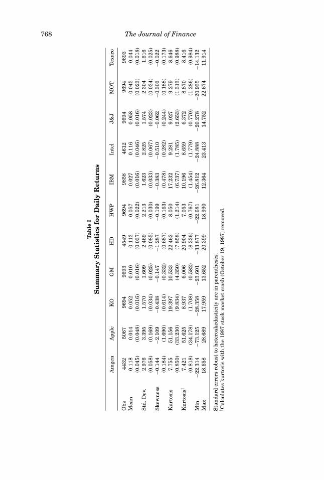
Table I provides summary statistics for daily continuously compounded re-turns for these firms. Percent returns were computed based on daily clos-ing prices, which have been adjusted for all applicable splits and dividenddistributions.
768 The Journal of Finance
Tab
leI
Su
mm
ary
Sta
tist
ics
for
Dai
lyR
etu
rns
Am
gen
App
leK
OG
MH
DH
WP
IBM
Inte
lJ&
JM
OT
Tex
aco
Obs
4432
5067
9694
9693
4549
9694
9858
4612
9694
9694
9693
Mea
n0.
118
0.01
40.
052
0.01
00.
113
0.05
70.
027
0.11
60.
058
0.04
50.
044
(0.0
45)
(0.0
48)
(0.0
16)
(0.0
16)
(0.0
37)
(0.0
22)
(0.0
16)
(0.0
46)
(0.0
16)
(0.0
23)
(0.0
18)
Std
.Dev
.2.
976
3.39
51.
570
1.60
92.
469
2.21
31.
623
2.82
51.
574
2.30
41.
616
(0.0
58)
(0.1
69)
(0.0
34)
(0.0
25)
(0.0
85)
(0.0
30)
(0.0
33)
(0.0
67)
(0.0
23)
(0.0
34)
(0.0
25)
Ske
wn
ess
−0.1
44−2
.109
−0.4
38−0
.147
−1.2
87−0
.199
−0.3
83−0
.510
−0.0
62−0
.303
−0.0
22(0
.184
)(1
.690
)(0
.614
)(0
.332
)(0
.687
)(0
.163
)(0
.478
)(0
.282
)(0
.244
)(0
.188
)(0
.173
)K
urt
osis
7.75
551
.156
19.3
9710
.533
22.4
628.
050
17.2
329.
281
9.02
79.
279
8.64
6(0
.850
)(3
3.23
0)(9
.834
)(4
.350
)(7
.858
)(1
.214
)(6
.737
)(1
.785
)(2
.653
)(1
.313
)(0
.988
)K
urt
osis
†7.
421
51.6
258.
937
6.00
620
.904
7.05
310
.196
8.65
96.
372
8.87
08.
416
(0.8
18)
(34.
178)
(1.7
08)
(0.5
82)
(8.3
36)
(0.7
67)
(1.4
54)
(1.7
79)
(0.7
70)
(1.2
86)
(0.9
84)
Min
−22.
314
−73.
125
−28.
358
−23.
601
−33.
877
−22.
681
−26.
812
−24.
888
−20.
278
−20.
935
−14.
132
Max
18.6
5828
.689
17.9
5913
.652
20.3
9918
.990
12.3
6423
.413
14.7
5222
.674
11.9
14
Sta
nda
rder
rors
robu
stto
het
eros
keda
stic
ity
are
inpa
ren
thes
es.
† Cal
cula
tes
kurt
osis
wit
hth
e19
87st
ock
mar
ket
cras
h(O
ctob
er19
,198
7)re
mov
ed.
Individual Stock Returns 769
III. Results for the GARJI Model
A. Individual Firms
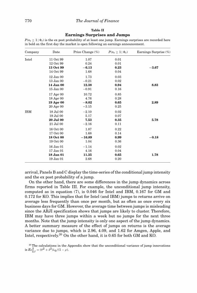
This subsection discusses estimation results for our GARCH-jump modelwith autoregressive jump intensity (GARJI) applied to individual firms. Table IIreports some empirical evidence supporting the conjecture that important newsevents, such as earnings surprises, can be a source of jumps. Choosing Intel andIBM as examples, and using the last six quarters of our sample, Table II reportsearnings surprises,19 daily price changes, and the probability that at least onejump occurred. For example, the large price drop for IBM on October 18, 2000was associated with a 0.99 probability of at least one jump and a negative earn-ings surprise reported the night before. Another interesting example was April2000 for Intel. Our model inferred that a jump occurred on April 17. The 10.72percent return that day may have been in anticipation of the positive earningssurprise reported the next day after the market closed. However, following theearnings announcement, there was another jump associated with a return of−8.02. One possible interpretation was that the positive earnings surprise wasnot as large as the market had anticipated. This example illustrates how jumpscan be clustered around significant news events. Of course earnings surprisesare only one source of news innovations that are associated with jumps. As dis-cussed further below, another source, which often results in a cluster of jumpsis a market crash such as October 1987.
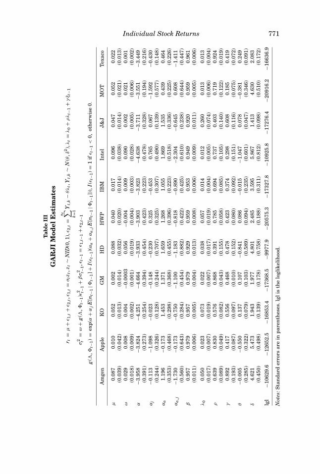
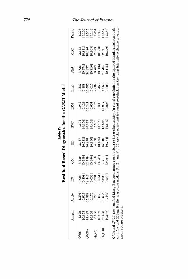
Table III reports parameter estimates for our GARJI model applied to in-dividual firms. The residual-based diagnostic test results reported in Table IVindicate that there is no remaining serial correlation in either the squared stan-dardized residuals or the jump intensity residuals. It is useful to note that thelatter test indicated misspecification for the case of a constant intensity param-eter (λt = λ). Also, a likelihood ratio (LR) test for the ARJI versus a constantjump intensity model strongly favors the ARJI dynamics for all models. The LRtests are discussed in more detail in the next section.
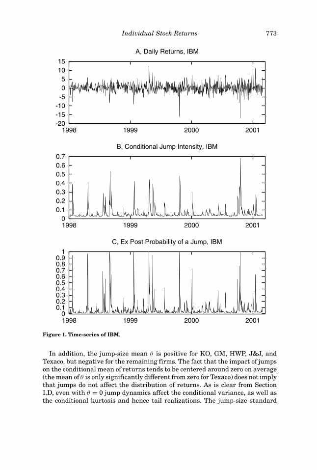
There are several common features for all companies evident in the Table IIIresults. First, there is very significant evidence of time-variation in the arrivalof jump events (ρ and γ are both significantly different from zero) for all firms.Note that the persistence parameter ρ for the arrival of jump events (jump clus-tering) is quite high, although it is considerably lower for J&J, HD, and KO thanfor all of the other firms. Secondly, the parameter γ , which measures the effectof the most recent intensity residual (the change in the conditional forecast ofnt−1 due to last day’s information innovation) ranges from 0.185 to 0.892. Thisstatistical significance of both the lagged intensity residual and jump clusteringsuggests that the arrival process can systematically deviate from its uncondi-tional mean. Panels A to E in Figure 1 display several features of the modelfor IBM over the recent period 1998 to 2001. For example, pertaining to jump
19 Earnings surprises were obtained from Bloomberg; they are based on the average of analysts’forecasts reported by IBES.
770 The Journal of Finance
Table IIEarnings Surprises and Jumps
P(nt ≥ 1 | �t) is the ex post probability of at least one jump. Earnings surprises are recorded herein bold on the first day the market is open following an earnings announcement.
Company Date Price Change (%) P(nt ≥ 1 | �t) Earnings Surprise (%)
Intel 11 Oct 99 1.07 0.0112 Oct 99 0.24 0.0113 Oct 99 −6.13 0.23 −3.6714 Oct 99 1.68 0.04
12 Jan 00 1.73 0.0313 Jan 00 −0.21 0.0214 Jan 00 12.38 0.94 8.8315 Jan 00 −0.91 0.16
17 Apr 00 10.72 0.8518 Apr 00 4.76 0.2819 Apr 00 −8.02 0.65 2.8920 Apr 00 −3.15 0.25
IBM 18 Jul 00 −2.10 0.0219 Jul 00 5.17 0.0720 Jul 00 7.53 0.35 5.7821 Jul 00 −2.16 0.11
16 Oct 00 1.87 0.2217 Oct 00 1.68 0.1418 Oct 00 −16.89 0.99 −0.1819 Oct 00 1.04 0.36
16 Jan 01 −1.14 0.0217 Jan 01 4.16 0.0418 Jan 01 11.35 0.65 1.7819 Jan 01 2.68 0.20
arrival, Panels B and C display the time-series of the conditional jump intensityand the ex post probability of a jump.
On the other hand, there are some differences in the jump dynamics acrossfirms reported in Table III. For example, the unconditional jump intensity,computed as in equation (7), is 0.046 for Intel and IBM, 0.167 for GM and0.172 for KO. This implies that for Intel (and IBM) jumps to returns arrive onaverage less frequently than once per month, but as often as once every sixbusiness days for GM. However, the average time between jumps is misleadingsince the ARJI specification shows that jumps are likely to cluster. Therefore,IBM may have three jumps within a week but no jumps for the next threemonths. Note that the jump intensity is only one aspect of the jump dynamics.A better summary measure of the effect of jumps on returns is the averagevariance due to jumps, which is 2.96, 4.09, and 1.62 for Amgen, Apple, andIntel, respectively.20 On the other hand, it is 0.65 for both GM and KO.
20 The calculations in the Appendix show that the unconditional variance of jump innovationsis Eε2
2,t = (θ2 + δ2)λ0/(1 − ρ).
Individual Stock Returns 771
Tab
leII
IG
AR
JI
Mod
elE
stim
ates
r t=
µ+
ε 1,t
+ε 2
,t,ε
1,t=
σtz
t,z t
∼N
ID(0
,1),
ε 2,t
=n t ∑ k=
1
Yt,
k−
θλ
t,Y
t,k
∼N
(θ,δ
2),
λt=
λ0
+ρλ
t−1
+γξ t
−1
σ2 t
=ω
+g
(�,�
t−1)ε
2 t−1
+βσ
2 t−1,ε
t−1
=ε 1
,t−1
+ε 2
,t−1
g(�
,�t−
1)
=ex
p(α
+α
jE
[nt−
1|�
t−1]+
I(ε t
−1)(
αa
+α
a,jE
[nt−
1|�
t−1])
),I(
ε t−1
)=
1if
ε t−1
<0,
oth
erw
ise
0.
Am
gen
App
leK
OG
MH
DH
WP
IBM
Inte
lJ&
JM
OT
Tex
aco
µ0.
087
0.01
00.
052
0.00
20.
088
0.04
00.
017
0.09
60.
047
0.05
20.
022
(0.0
39)
(0.0
42)
(0.0
13)
(0.0
14)
(0.0
32)
(0.0
20)
(0.0
14)
(0.0
38)
(0.0
14)
(0.0
21)
(0.0
13)
ω0.
029
0.00
80.
004
−0.0
003
0.05
6−0
.004
0.00
90.
090
0.00
20.
021
0.00
1(0
.018
)(0
.009
)(0
.002
)(0
.001
)(0
.019
)(0
.004
)(0
.003
)(0
.028
)(0
.005
)(0
.006
)(0
.002
)α
−3.9
58−3
.824
−4.2
51−4
.664
−3.9
33−3
.903
−3.8
23−4
.638
−3.7
11−3
.551
−3.4
49(0
.391
)(0
.273
)(0
.254
)(0
.394
)(0
.454
)(0
.423
)(0
.223
)(0
.478
)(0
.328
)(0
.194
)(0
.216
)α
j−0
.113
−1.0
98−0
.023
−0.1
48−0
.230
0.32
5−0
.453
0.76
50.
067
−1.5
92−0
.430
(0.2
44)
(0.3
26)
(0.1
28)
(0.2
44)
(0.7
07)
(0.3
25)
(0.3
07)
(0.4
90)
(0.1
39)
(0.5
77)
(0.1
48)
αa
1.19
6−0
.173
1.45
31.
371
1.65
91.
268
1.05
51.
869
1.53
50.
439
0.46
4(0
.353
)(0
.468
)(0
.298
)(0
.368
)(0
.455
)(0
.396
)(0
.223
)(0
.518
)(0
.336
)(0
.225
)(0
.226
)α
a,j
−1.7
30−0
.173
−0.7
50−1
.100
−1.1
83−0
.818
−0.8
90−2
.304
−0.6
450.
608
−1.4
11(0
.560
)(0
.643
)(0
.284
)(0
.454
)(0
.882
)(0
.422
)(0
.425
)(0
.610
)(0
.238
)(0
.644
)(0
.447
)β
0.95
70.
979
0.95
70.
979
0.92
90.
959
0.95
30.
949
0.92
00.
959
0.96
1(0
.011
)(0
.006
)(0
.005
)(0
.004
)(0
.013
)(0
.008
)(0
.006
)(0
.009
)(0
.011
)(0
.005
)(0
.006
)
λ0
0.05
00.
023
0.07
30.
022
0.03
80.
057
0.01
40.
012
0.26
00.
013
0.01
3(0
.017
)(0
.007
)(0
.019
)(0
.007
)(0
.017
)(0
.019
)(0
.004
)(0
.005
)(0
.074
)(0
.006
)(0
.004
)ρ
0.63
90.
830
0.57
60.
868
0.39
10.
785
0.69
40.
737
0.40
30.
719
0.92
4(0
.089
)(0
.049
)(0
.082
)(0
.043
)(0
.155
)(0
.058
)(0
.085
)(0
.105
)(0
.140
)(0
.122
)(0
.019
)γ
0.89
20.
417
0.55
60.
468
0.47
80.
423
0.37
40.
298
0.60
80.
185
0.41
9(0
.193
)(0
.087
)(0
.097
)(0
.010
)(0
.152
)(0
.080
)(0
.092
)(0
.151
)(0
.116
)(0
.075
)(0
.072
)θ
−0.0
05−0
.550
0.13
70.
107
−0.8
410.
086
−0.0
15−1
.047
0.07
8−0
.381
0.24
9(0
.285
)(0
.322
)(0
.079
)(0
.103
)(0
.589
)(0
.094
)(0
.235
)(0
.601
)(0
.047
)(0
.346
)(0
.091
)δ
4.62
15.
473
1.94
31.
977
4.80
12.
485
3.59
55.
867
1.41
34.
630
2.08
3(0
.450
)(0
.498
)(0
.139
)(0
.178
)(0
.758
)(0
.188
)(0
.311
)(0
.812
)(0
.098
)(0
.510
)(0
.172
)
lgl
−106
29.6
−126
52.5
−168
53.4
−173
68.5
−997
7.9
−205
75.3
−173
27.8
−109
25.8
−172
76.4
−209
16.2
−166
36.9
Not
es:S
tan
dard
erro
rsar
ein
pare
nth
eses
.lgl
isth
elo
glik
elih
ood.
772 The Journal of Finance
Tab
leIV
Res
idu
al-B
ased
Dia
gnos
tics
for
the
GA
RJ
IM
odel
Am
gen
App
leK
OG
MH
DH
WP
IBM
Inte
lJ&
JM
OT
Tex
aco
Q2(5
)1.
825
1.39
25.
065
3.72
92.
467
1.80
14.
942
5.23
73.
828
2.19
89.
223
[0.8
73]
[0.9
25]
[0.4
08]
[0.5
89]
[0.7
81]
[0.8
76]
[0.4
23]
[0.3
88]
[0.5
74]
[0.8
21]
[0.1
00]
Q2(2
0)14
.437
25.8
6233
.447
12.7
8910
.395
20.8
1717
.341
17.5
8524
.637
10.2
8626
.575
[0.8
08]
[0.1
70]
[0.0
30]
[0.8
86]
[0.9
60]
[0.4
08]
[0.6
31]
[0.6
15]
[0.2
16]
[0.9
63]
[0.1
48]
Qξ t
(5)
5.50
63.
276
3.99
12.
016
4.92
32.
939
5.17
54.
662
3.75
22.
079
5.21
4[0
.357
][0
.658
][0
.551
][0
.847
][0
.425
][0
.709
][0
.395
][0
.458
][0
.586
][0
.838
][0
.390
]Q
ξ t(2
0)32
.625
19.5
3518
.603
7.71
715
.040
18.8
4624
.917
14.0
5327
.764
22.9
7116
.487
[0.0
37]
[0.4
87]
[0.5
48]
[0.9
94]
[0.7
74]
[0.5
32]
[0.2
05]
[0.8
28]
[0.1
15]
[0.2
90]
[0.6
86]
Q2(5
)an
dQ
2(2
0)ar
em
odif
ied
Lju
ng-
Box
port
man
teau
test
,rob
ust
toh
eter
oske
dast
icit
y,fo
rse
rial
corr
elat
ion
inth
esq
uar
edst
anda
rdiz
edre
sidu
als
wit
hfi
vean
d20
lags
for
the
resp
ecti
vem
odel
s.Q
ξ t(5
),an
dQ
ξ t(2
0)ar
eth
esa
me
test
for
seri
alco
rrel
atio
nin
the
jum
pin
ten
sity
resi
dual
s.p-
valu
esar
ein
squ
are
brac
kets
.
Individual Stock Returns 773
-20-15-10-5 0 5
10 15
1998 1999 2000 2001
A, Daily Returns, IBM
0 0.1 0.2 0.3 0.4 0.5 0.6 0.7
1998 1999 2000 2001
B, Conditional Jump Intensity, IBM
0 0.1 0.2 0.3 0.4 0.5 0.6 0.7 0.8 0.9
1
1998 1999 2000 2001
C, Ex Post Probability of a Jump, IBM
Figure 1. Time-series of IBM.
In addition, the jump-size mean θ is positive for KO, GM, HWP, J&J, andTexaco, but negative for the remaining firms. The fact that the impact of jumpson the conditional mean of returns tends to be centered around zero on average(the mean of θ is only significantly different from zero for Texaco) does not implythat jumps do not affect the distribution of returns. As is clear from SectionI.D, even with θ = 0 jump dynamics affect the conditional variance, as well asthe conditional kurtosis and hence tail realizations. The jump-size standard
774 The Journal of Finance
0 2 4 6 8
10 12 14 16 18
1998 1999 2000 2001
D, Conditional Variance, IBM
0 2 4 6 8
10 12 14
1998 1999 2000 2001
E, Conditional Variance Components, IBM
GARCH componentJump component
Figure 1.—Continued
deviation δ is larger for Intel, Apple, and Amgen. Results in Section III.B willinvestigate whether there is a general difference between new economy andtraditional economy stocks with respect to size and average jump direction(sign of the jump-size mean).
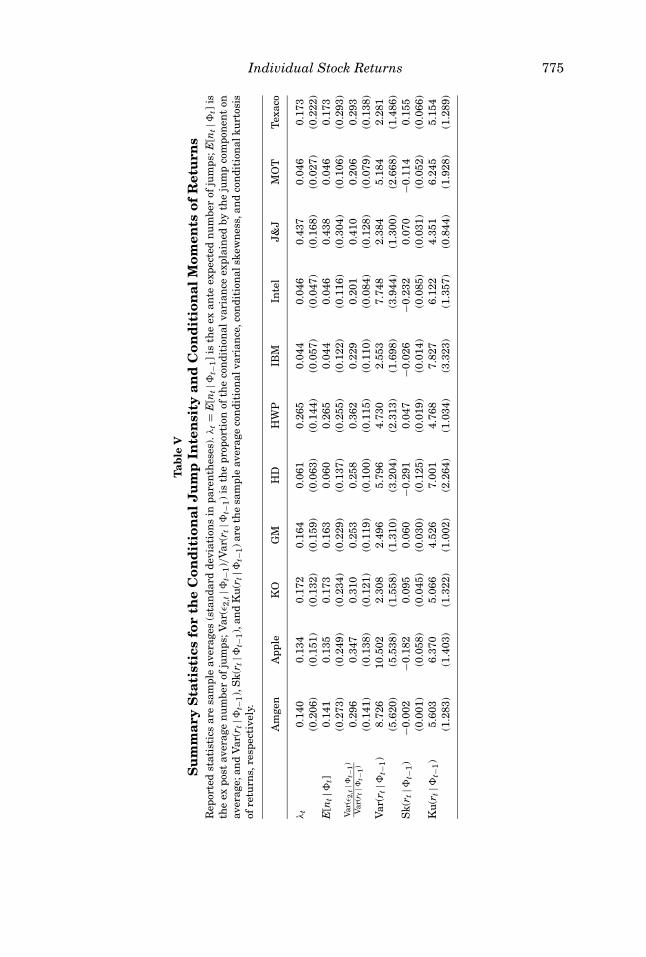
Table V reports some descriptive statistics for the jump components. The sam-ple averages of λt for the firms are almost identical to the implied unconditionalnumber of jumps (equation (7)) discussed above. The average realized numberof jumps per period (mean of E[nt | �t]) is very close to the average expectednumber of jumps (mean of λt) for each firm indicating that the λt are unbiasedforecasts for E[nt | �t]. As expected, the ex post measure of the number of jumpsE[nt | �t], has a higher standard deviation than its ex ante component, λt.
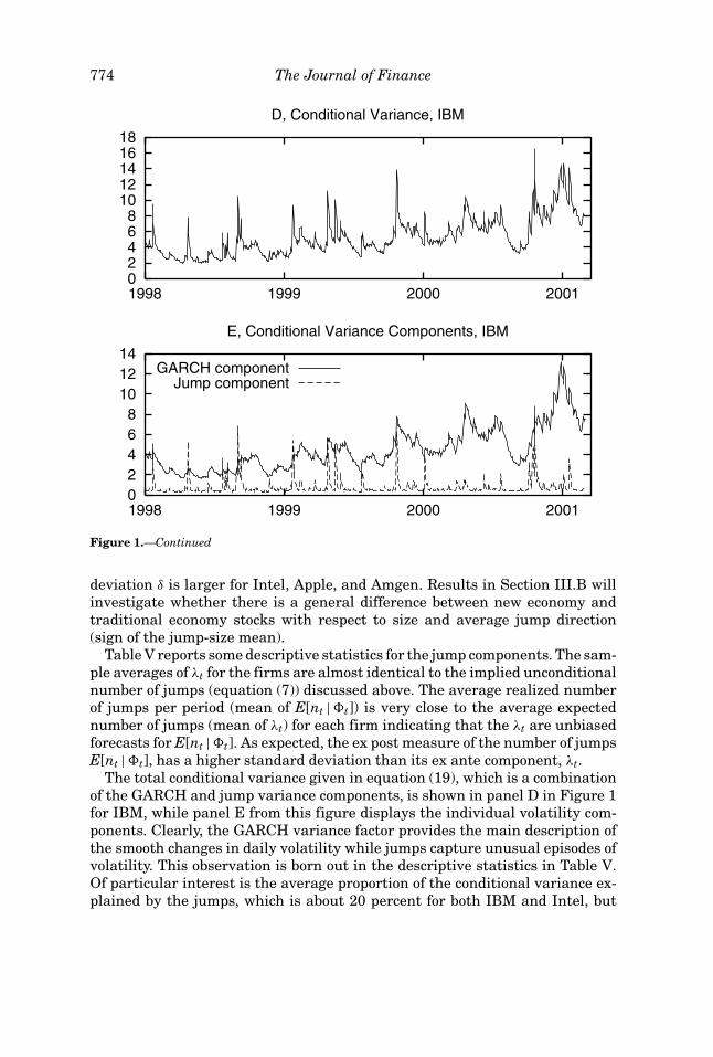
The total conditional variance given in equation (19), which is a combinationof the GARCH and jump variance components, is shown in panel D in Figure 1for IBM, while panel E from this figure displays the individual volatility com-ponents. Clearly, the GARCH variance factor provides the main description ofthe smooth changes in daily volatility while jumps capture unusual episodes ofvolatility. This observation is born out in the descriptive statistics in Table V.Of particular interest is the average proportion of the conditional variance ex-plained by the jumps, which is about 20 percent for both IBM and Intel, but
Individual Stock Returns 775
Tab
leV
Su
mm
ary
Sta
tist
ics
for
the
Con
dit
ion
alJ
um
pIn
ten
sity
and
Con
dit
ion
alM
omen
tsof
Ret
urn
sR
epor
ted
stat
isti
csar
esa
mpl
eav
erag
es(s
tan
dard
devi
atio
ns
inpa
ren
thes
es).
λt=
E[n
t|�
t−1]
isth
eex
ante
expe
cted
nu
mbe
rof
jum
ps;E
[nt|�
t]is
the
expo
stav
erag
en
um
ber
ofju
mps
;Var
(ε2,
t|�
t−1)/
Var
(rt|�
t−1)
isth
epr
opor
tion
ofth
eco
ndi
tion
alva
rian
ceex
plai
ned
byth
eju
mp
com
pon
ent
onav
erag
e;an
dV
ar(r
t|�
t−1),
Sk(
r t|�
t−1),
and
Ku
(rt|�
t−1)a
reth
esa
mpl
eav
erag
eco
ndi
tion
alva
rian
ce,c
ondi
tion
alsk
ewn
ess,
and
con
diti
onal
kurt
osis
ofre
turn
s,re
spec
tive
ly.
Am
gen
App
leK
OG
MH
DH
WP
IBM
Inte
lJ&
JM
OT
Tex
aco
λt
0.14
00.
134
0.17
20.
164
0.06
10.
265
0.04
40.
046
0.43
70.
046
0.17
3(0
.206
)(0
.151
)(0
.132
)(0
.159
)(0
.063
)(0
.144
)(0
.057
)(0
.047
)(0
.168
)(0
.027
)(0
.222
)E
[nt|�
t]0.
141
0.13
50.
173
0.16
30.
060
0.26
50.
044
0.04
60.
438
0.04
60.
173
(0.2
73)
(0.2
49)
(0.2
34)
(0.2
29)
(0.1
37)
(0.2
55)
(0.1
22)
(0.1
16)
(0.3
04)
(0.1
06)
(0.2
93)
Var
(ε2,
t|�
t−1)
Var
(rt|�
t−1)
0.29
60.
347
0.31
00.
253
0.25
80.
362
0.22
90.
201
0.41
00.
206
0.29
3(0
.141
)(0
.138
)(0
.121
)(0
.119
)(0
.100
)(0
.115
)(0
.110
)(0
.084
)(0
.128
)(0
.079
)(0
.138
)V
ar(r
t|�
t−1)
8.72
610
.502
2.30
82.
496
5.79
64.
730
2.55
37.
748
2.38
45.
184
2.28
1(5
.620
)(5
.538
)(1
.558
)(1
.310
)(3
.204
)(2
.313
)(1
.698
)(3
.944
)(1
.300
)(2
.668
)(1
.486
)S
k(r t
|�t−
1)
−0.0
02−0
.182
0.09
50.
060
−0.2
910.
047
−0.0
26−0
.232
0.07
0−0
.114
0.15
5(0
.001
)(0
.058
)(0
.045
)(0
.030
)(0
.125
)(0
.019
)(0
.014
)(0
.085
)(0
.031
)(0
.052
)(0
.066
)K
u(r
t|�
t−1)
5.60
36.
370
5.06
64.
526
7.00
14.
768
7.82
76.
122
4.35
16.
245
5.15
4(1
.283
)(1
.403
)(1
.322
)(1
.002
)(2
.264
)(1
.034
)(3
.323
)(1
.357
)(0
.844
)(1
.928
)(1
.289
)
776 The Journal of Finance
30 percent for Texaco and 40 percent for J&J. However, at times as much as90 percent of the conditional variance for Amgen is due to the jump component.
As previously noted, jumps will contribute to conditional skewness and kur-tosis. Table V reports the average conditional skewness and kurtosis impliedby the model. Even in the case of companies that have a relatively low numberof jumps, the effects on higher conditional moments can be substantial. Forinstance, over the period 1990 to 1992 there is considerable variation in condi-tional kurtosis for Intel, reaching as high as 13 and spending most of the time inthe range of five to nine. Equation (21) indicates that when λt > 0, the GARCHvariance component will have an effect on conditional kurtosis, in contrast to amodel without jumps, which has a constant conditional kurtosis.
A.1. The Effect of Jumps on Expected Volatility
Traditional jump diffusion models assume the process governing jump ar-rivals is independently and identically distributed and do not allow jumps toaffect the dynamics of diffusion volatility. In our case, jumps can affect expectedvolatility through two channels. Firstly, jumps affect the conditional variancedirectly through the time-varying Poisson arrival process and contribute to timevariation in the second- and higher-order moments. Secondly, the GARCH com-ponent of the conditional variance includes the propagation effects of previouslyrealized jumps.
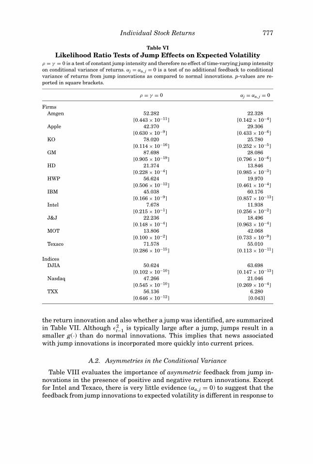
Table VI summarizes statistical tests of whether or not jumps affect volatilitydynamics. The first column of Table VI reports LR test statistics associatedwith the hypothesis that ρ = γ = 0. This test is designed to detect whetheror not time-variation in the jump intensity contributes to expected volatility.As expected from the t-statistics associated with these parameter estimates inTable III, these LR test results strongly reject ρ = γ = 0 so that jump clusteringaffects the conditional variance through this channel.
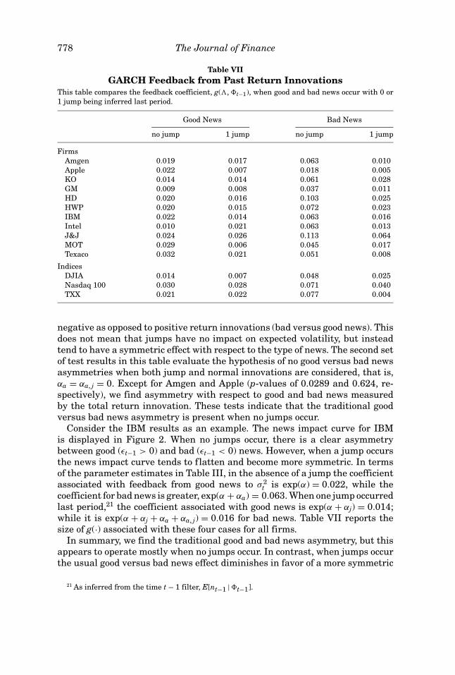
The results in the second column of Table VI refer to a LR test for the effectof jumps on conditional variance through GARCH feedback effects, that is, thepropagation of previously realized jump innovations to expected volatility. Ifthe parameters αj = αa, j = 0, then past jump innovations have the same effecton expected volatility as normal innovations. For all firms, we reject this nullhypothesis and conclude that jumps affect expected volatility differently thannormal innovations. Therefore, jumps do affect the conditional variance throughthis channel, and as shown in columns 2 and 4 of Table VII, tend to have asmaller positive feedback coefficient than do normal innovations.
Recall that εt−1 contains both normal and jump innovations that feed backinto the GARCH component of volatility. The feedback coefficient g(·), associatedwith ε2
t−1 in the GARCH function, includes the extra term αj when good newsand at least one jump occurs, and the extra terms αj + αa, j when a jump andbad news occurs. As reported in Table III, in nine out of the 11 firms, αj < 0reducing g(·) when a jump and good news occurs. Furthermore, when the newswas bad and a jump occured, all firms experience a reduction in g(·) sinceαj + αa, j < 0. The implications for the size of g(·), which depends on the sign of
Individual Stock Returns 777
Table VILikelihood Ratio Tests of Jump Effects on Expected Volatility
ρ = γ = 0 is a test of constant jump intensity and therefore no effect of time-varying jump intensityon conditional variance of returns. αj = αa, j = 0 is a test of no additional feedback to conditionalvariance of returns from jump innovations as compared to normal innovations. p-values are re-ported in square brackets.
ρ = γ = 0 αj = αa, j = 0
FirmsAmgen 52.282 22.328
[0.443 × 10⁻¹¹] [0.142 × 10⁻⁴]Apple 42.370 29.306
[0.630 × 10⁻⁹] [0.433 × 10⁻⁶]KO 78.020 25.780
[0.114 × 10⁻¹⁶] [0.252 × 10⁻⁵]GM 87.698 28.086
[0.905 × 10⁻¹⁹] [0.796 × 10⁻⁶]HD 21.374 13.846
[0.228 × 10⁻⁴] [0.985 × 10⁻³]HWP 56.624 19.970
[0.506 × 10⁻¹²] [0.461 × 10⁻⁴]IBM 45.038 60.176
[0.166 × 10⁻⁹] [0.857 × 10⁻¹³]Intel 7.678 11.938
[0.215 × 10⁻¹] [0.256 × 10⁻²]J&J 22.236 18.496
[0.148 × 10⁻⁴] [0.963 × 10⁻⁴]MOT 13.806 42.068
[0.100 × 10⁻²] [0.733 × 10⁻⁹]Texaco 71.578 55.010
[0.286 × 10⁻¹⁵] [0.113 × 10⁻¹¹]
IndicesDJIA 50.624 63.698
[0.102 × 10⁻¹⁰] [0.147 × 10⁻¹³]Nasdaq 47.266 21.046
[0.545 × 10⁻¹⁰] [0.269 × 10−4]TXX 56.136 6.280
[0.646 × 10⁻¹²] [0.043]
the return innovation and also whether a jump was identified, are summarizedin Table VII. Although ε2
t−1 is typically large after a jump, jumps result in asmaller g(·) than do normal innovations. This implies that news associatedwith jump innovations is incorporated more quickly into current prices.
A.2. Asymmetries in the Conditional Variance
Table VIII evaluates the importance of asymmetric feedback from jump in-novations in the presence of positive and negative return innovations. Exceptfor Intel and Texaco, there is very little evidence (αa, j = 0) to suggest that thefeedback from jump innovations to expected volatility is different in response to
778 The Journal of Finance
Table VIIGARCH Feedback from Past Return Innovations
This table compares the feedback coefficient, g(�, �t−1), when good and bad news occur with 0 or1 jump being inferred last period.
Good News Bad News
no jump 1 jump no jump 1 jump
FirmsAmgen 0.019 0.017 0.063 0.010Apple 0.022 0.007 0.018 0.005KO 0.014 0.014 0.061 0.028GM 0.009 0.008 0.037 0.011HD 0.020 0.016 0.103 0.025HWP 0.020 0.015 0.072 0.023IBM 0.022 0.014 0.063 0.016Intel 0.010 0.021 0.063 0.013J&J 0.024 0.026 0.113 0.064MOT 0.029 0.006 0.045 0.017Texaco 0.032 0.021 0.051 0.008
IndicesDJIA 0.014 0.007 0.048 0.025Nasdaq 100 0.030 0.028 0.071 0.040TXX 0.021 0.022 0.077 0.004
negative as opposed to positive return innovations (bad versus good news). Thisdoes not mean that jumps have no impact on expected volatility, but insteadtend to have a symmetric effect with respect to the type of news. The second setof test results in this table evaluate the hypothesis of no good versus bad newsasymmetries when both jump and normal innovations are considered, that is,αa = αa, j = 0. Except for Amgen and Apple (p-values of 0.0289 and 0.624, re-spectively), we find asymmetry with respect to good and bad news measuredby the total return innovation. These tests indicate that the traditional goodversus bad news asymmetry is present when no jumps occur.
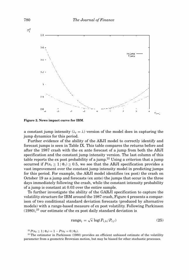
Consider the IBM results as an example. The news impact curve for IBMis displayed in Figure 2. When no jumps occur, there is a clear asymmetrybetween good (εt−1 > 0) and bad (εt−1 < 0) news. However, when a jump occursthe news impact curve tends to flatten and become more symmetric. In termsof the parameter estimates in Table III, in the absence of a jump the coefficientassociated with feedback from good news to σ 2
t is exp(α) = 0.022, while thecoefficient for bad news is greater, exp(α + αa) = 0.063. When one jump occurredlast period,21 the coefficient associated with good news is exp(α + αj) = 0.014;while it is exp(α + αj + αa + αa, j) = 0.016 for bad news. Table VII reports thesize of g(·) associated with these four cases for all firms.
In summary, we find the traditional good and bad news asymmetry, but thisappears to operate mostly when no jumps occur. In contrast, when jumps occurthe usual good versus bad news effect diminishes in favor of a more symmetric
21 As inferred from the time t − 1 filter, E[nt−1 | �t−1].
Individual Stock Returns 779
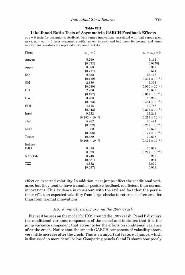
Table VIIILikelihood Ratio Tests of Asymmetric GARCH Feedback Effects
αa, j = 0 tests for asymmetric feedback from jumps innovations associated with bad versus goodnews. αa = αa, j = 0 tests asymmetry with respect to good and bad news for normal and jumpinnovations. p-values are reported in square brackets.
Firms αa, j = 0 αa = αa, j = 0
Amgen 5.260 7.162[0.022] [0.0278]
Apple 0.080 0.942[0.777] [0.624]
KO 2.552 25.428[0.110] [0.301 × 10⁻⁵]
GM 2.886 9.378[0.089] [0.920 × 10⁻²]
HD 2.206 10.020[0.137] [0.667 × 10⁻²]
HWP 3.208 15.266[0.073] [0.484 × 10⁻³]
IBM 4.118 30.788[0.042] [0.206 × 10⁻⁶]
Intel 9.622 12.244[0.192 × 10⁻²] [0.219 × 10⁻²]
J&J 5.282 30.494[0.022] [0.239 × 10⁻⁶]
MOT 1.080 12.670[0.298] [0.177 × 10⁻²]
Texaco 10.680 10.698[0.108 × 10⁻²] [0.475 × 10⁻²]
IndicesDJIA 0.018 30.062
0.893 [0.297 × 10⁻⁶]NASDAQ 0.748 6.260
[0.387] [0.044]TXX 4.882 6.800
[0.027] [0.033]
effect on expected volatility. In addition, past jumps affect the conditional vari-ance, but they tend to have a smaller positive feedback coefficient than normalinnovations. This evidence is consistent with the stylized fact that the persis-tence effect on expected volatility from large shocks to returns is often smallerthan from normal innovations.
A.3. Jump Clustering around the 1987 Crash
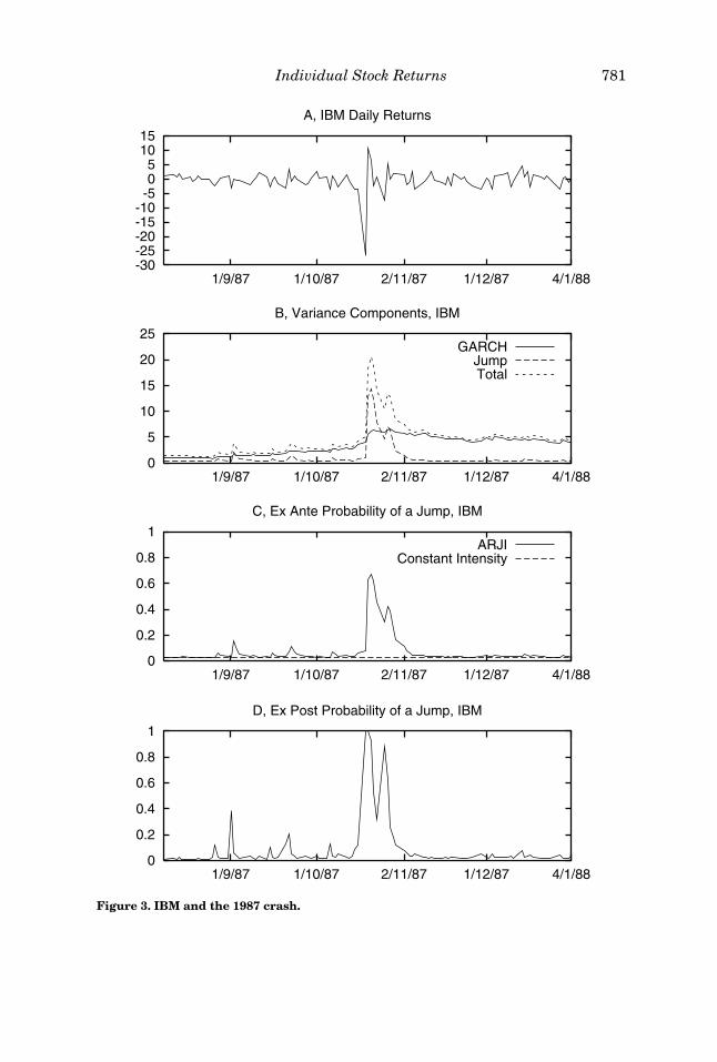
Figure 3 focuses on the model for IBM around the 1987 crash. Panel B displaysthe conditional variance components of the model and indicates that it is thejump variance component that accounts for the effects on conditional varianceafter the crash. Notice that the smooth GARCH component of volatility showsvery little increase after the crash. This is an important feature of jumps, whichis discussed in more detail below. Comparing panels C and D shows how poorly
780 The Journal of Finance
Figure 2. News impact curve for IBM.
a constant jump intensity (λt = λ) version of the model does in capturing thejump dynamics for this period.
Further evidence of the ability of the ARJI model to correctly identify andforecast jumps is seen in Table IX. This table compares the returns before andafter the 1987 crash with the ex ante forecast of a jump from both the ARJIspecification and the constant jump intensity version. The last column of thistable reports the ex post probability of a jump.22 Using a criterion that a jumpoccurred if P(nt ≥ 1 | �t) ≥ 0.5, we see that the ARJI specification provides avast improvement over the constant jump intensity model in predicting jumpsfor this period. For example, the ARJI model identifies (ex post) the crash onOctober 19 as a jump and forecasts (ex ante) the jumps that occur in the threedays immediately following the crash, while the constant intensity probabilityof a jump is constant at 0.03 over the entire sample.
To further investigate the ability of the GARJI specification to capture thevolatility structure for IBM around the 1987 crash, Figure 4 presents a compar-ison of two conditional standard deviation forecasts (produced by alternativemodels) with a range-based measure of ex post volatility. Following Parkinson(1980),23 our estimate of the ex post daily standard deviation is
ranget = √κ log(Pt,h/Pt,l ) (25)
22 P(nt ≥ 1 | �t) = 1 − P(nt = 0 | �t).23 The estimator in Parkinson (1980) provides an efficient unbiased estimate of the volatility
parameter from a geometric Brownian motion, but may be biased for other stochastic processes.
Individual Stock Returns 781
-30-25-20-15-10-5 0 5
10 15
1/9/87 1/10/87 2/11/87 1/12/87 4/1/88
A, IBM Daily Returns
0
5
10
15
20
25
1/9/87 1/10/87 2/11/87 1/12/87 4/1/88
B, Variance Components, IBM
GARCHJumpTotal
0
0.2
0.4
0.6
0.8
1
1/9/87 1/10/87 2/11/87 1/12/87 4/1/88
C, Ex Ante Probability of a Jump, IBM
ARJIConstant Intensity
0
0.2
0.4
0.6
0.8
1
1/9/87 1/10/87 2/11/87 1/12/87 4/1/88
D, Ex Post Probability of a Jump, IBM
Figure 3. IBM and the 1987 crash.
782 The Journal of Finance
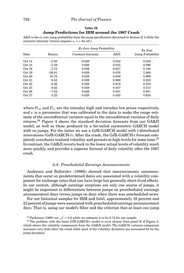
Table IXJump Predictions for IBM around the 1987 Crash
ARJI is the ex ante jump probability from the jump specification discussed in Section II.1 while theconstant intensity version imposes λt = λ for all t.
Ex Ante Jump ProbabilityEx Post
Date Return Constant Intensity ARJI Jump Probability
Oct 14 −2.38 0.029 0.032 0.032Oct 15 −3.59 0.029 0.035 0.090Oct 16 −3.72 0.029 0.057 0.120Oct 19 −26.81 0.029 0.076 1.000Oct 20 10.78 0.029 0.630 0.999Oct 21 6.52 0.029 0.669 0.923Oct 22 −2.26 0.029 0.618 0.532Oct 23 0.62 0.029 0.457 0.313Oct 26 −7.52 0.029 0.301 0.881Oct 27 5.22 0.029 0.420 0.624
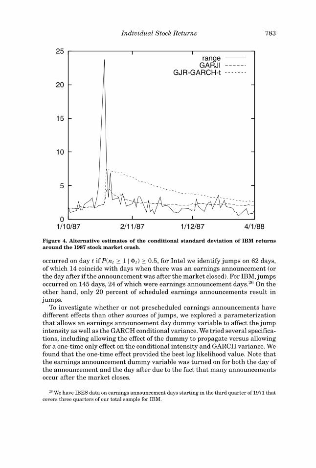
where Pt,h and Pt,l are the intraday high and intraday low prices respectively,and κ is a parameter that was calibrated to the data to make the range esti-mate of the unconditional variance equal to the unconditional variance of dailyreturns.24 Figure 4 shows the standard deviation forecasts from our GARJImodel, as well as those produced by a fat-tailed asymmetric GARCH modelwith no jumps. For the latter we use a GJR-GARCH model with t-distributedinnovations (GJR-GARCH-t). After the crash, the GJR-GARCH-t forecast com-pletely overshoots realized volatility and persists at high levels for some time.25
In contrast, the GARJI reverts back to the lower actual levels of volatility muchmore quickly, and provides a superior forecast of daily volatility after the 1987crash.
A.4. Prescheduled Earnings Announcements
Andersen and Bollerslev (1998b) showed that macroeconomic announce-ments that occur on predetermined dates are associated with a volatility com-ponent for exchange rates that can have large but generally short-lived effects.In our context, although earnings surprises are only one source of jumps, itmight be important to differentiate between jumps on prescheduled earningsannouncement days versus jumps on days when there was unscheduled news.
For our historical samples for IBM and Intel, approximately 16 percent and23 percent of jumps were associated with prescheduled earnings announcementdays. That is, using our model’s filter and the criterion that at least one jump
24 Parkinson (1980) set√
κ = 0.6 while we estimate it to be 0.74 for our sample.25 The problem with the basic GJR-GARCH-t model is even clearer from panel B of Figure 3,
which shows the volatility components from the GARJI model. The GARCH variance componentincreases very little after the crash while most of the volatility dynamics are accounted for by thejump dynamics.
Individual Stock Returns 783
0
5
10
15
20
25
1/10/87 2/11/87 1/12/87 4/1/88
rangeGARJI
GJR-GARCH-t
Figure 4. Alternative estimates of the conditional standard deviation of IBM returnsaround the 1987 stock market crash.
occurred on day t if P(nt ≥ 1 | �t) ≥ 0.5, for Intel we identify jumps on 62 days,of which 14 coincide with days when there was an earnings announcement (orthe day after if the announcement was after the market closed). For IBM, jumpsoccurred on 145 days, 24 of which were earnings announcement days.26 On theother hand, only 20 percent of scheduled earnings announcements result injumps.
To investigate whether or not prescheduled earnings announcements havedifferent effects than other sources of jumps, we explored a parameterizationthat allows an earnings announcement day dummy variable to affect the jumpintensity as well as the GARCH conditional variance. We tried several specifica-tions, including allowing the effect of the dummy to propagate versus allowingfor a one-time only effect on the conditional intensity and GARCH variance. Wefound that the one-time effect provided the best log likelihood value. Note thatthe earnings announcement dummy variable was turned on for both the day ofthe announcement and the day after due to the fact that many announcementsoccur after the market closes.
26 We have IBES data on earnings announcement days starting in the third quarter of 1971 thatcovers three quarters of our total sample for IBM.
784 The Journal of Finance
The results for this richer model are very comparable to our main resultsthat were discussed above and reported in Table III. In particular, all of ourconclusions, such as jump clustering and volatility asymmetries, are robust tothe addition of prescheduled announcement dummies. The effect of announce-ment dummies was imprecisely estimated for our data. As noted above, therelatively infrequent occurrence of announcements that result in jumps meanthat long samples are needed to accurately identify different types of jumpdynamics.
B. Indices
During discussion of the results for individual firms, it appeared as if theremight be differences between traditional firms and new economy firms. Giventhat available time-series are too short for many Internet stocks, and also thatit is difficult to classify some firms as traditional versus high-tech, this sectionreports results for our GARJI model applied to three different indices that coverdifferent types of firms. Table X reports parameter estimates for the GARJImodel for the DJIA, Nasdaq 100, and the CBOE Technology Index (TXX). Thespecification of the GARJI model in this table includes an AR(1) term to accountfor the autocorrelation found in the conditional mean of returns for the indices.27
The three indices cover the spectrum of volatility levels from low to high,ordered as DJIA, Nasdaq 100, and TXX. Unconditional standard deviations are0.948, 1.815, and 2.429 for the DJIA, Nasdaq, and TXX, respectively. Consistentwith this ordering is an increased likelihood of jumps for the more volatileindices. For instance, the implied unconditional jump intensities are 0.135,0.136, and 1.429 for the DJIA, Nasdaq 100, and TXX, respectively. The averagevariance due to jumps is 0.224 (DJIA), 0.443 (Nasdaq 100), and 5.073 (TXX). Themore volatile the index the larger the jump variance, although the proportionof the conditional variance explained by jumps is still quite low overall, 0.166for the DJIA, 0.144 for the Nasdaq 100, and 0.228 for the TXX index. Theseresults suggest that jumps in the DJIA are less frequent and have a smallereffect on returns than the other indices. Conversely, returns from the volatileTXX index display frequent large jumps.
There are several features that are common for individual firm and indexdynamics. For both, the addition of the ARJI jump dynamics provides a strongstatistical improvement over a constant jump intensity specification (see esti-mates for ρ and γ in Table X and column 1 of Table VI). The process governingthe arrival of jumps is serially correlated, which implies jump clustering for theindices as well. One difference between the individual firm results and those forthe two most volatile indices is that revisions to the conditional jump intensity,ξt−1, are more important for the latter. For example, γ is 0.936 and 0.974 forthe Nasdaq 100 and TXX, respectively, which is larger than the value for theDJIA and all the individual firms.
27 Market microstructure effects such as stale prices can cause low-order autocorrelation in indexreturns.
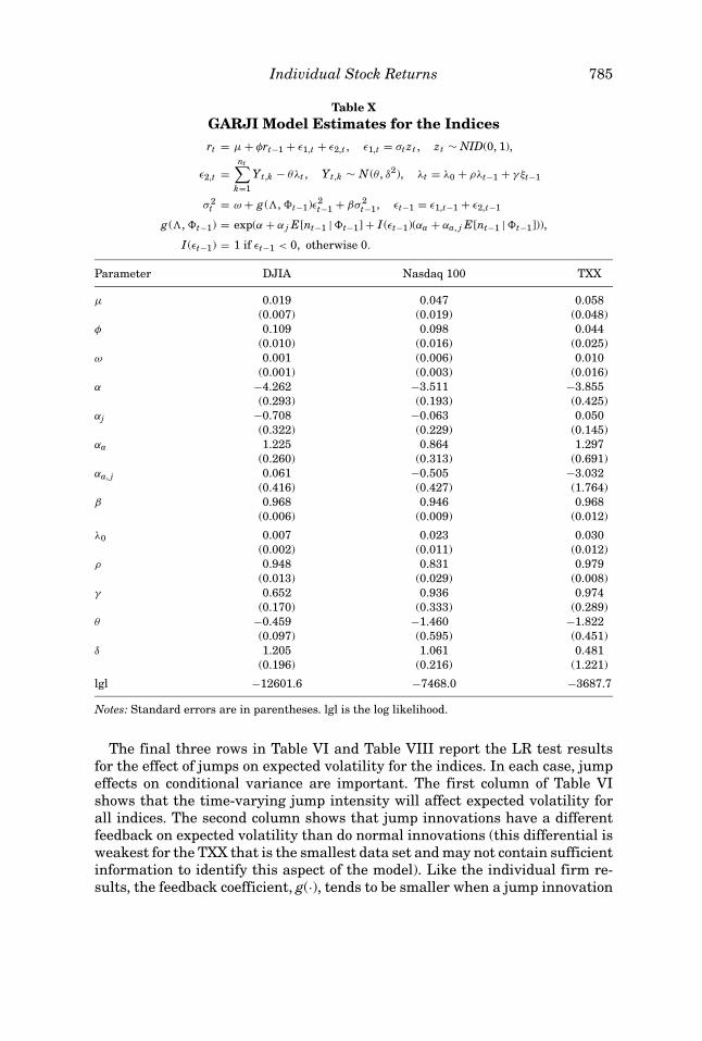
Individual Stock Returns 785
Table XGARJI Model Estimates for the Indicesrt = µ + φrt−1 + ε1,t + ε2,t , ε1,t = σt zt , zt ∼ NID(0, 1),
ε2,t =nt∑
k=1
Yt,k − θλt , Yt,k ∼ N (θ , δ2), λt = λ0 + ρλt−1 + γ ξt−1
σ 2t = ω + g (�, �t−1)ε2
t−1 + βσ 2t−1, εt−1 = ε1,t−1 + ε2,t−1
g (�, �t−1) = exp(α + α j E[nt−1 | �t−1] + I (εt−1)(αa + αa, j E[nt−1 | �t−1])),
I (εt−1) = 1 if εt−1 < 0, otherwise 0.
Parameter DJIA Nasdaq 100 TXX
µ 0.019 0.047 0.058(0.007) (0.019) (0.048)
φ 0.109 0.098 0.044(0.010) (0.016) (0.025)
ω 0.001 (0.006) 0.010(0.001) (0.003) (0.016)
α −4.262 −3.511 −3.855(0.293) (0.193) (0.425)
αj −0.708 −0.063 0.050(0.322) (0.229) (0.145)
αa 1.225 0.864 1.297(0.260) (0.313) (0.691)
αa, j 0.061 −0.505 −3.032(0.416) (0.427) (1.764)
β 0.968 0.946 0.968(0.006) (0.009) (0.012)
λ0 0.007 0.023 0.030(0.002) (0.011) (0.012)
ρ 0.948 0.831 0.979(0.013) (0.029) (0.008)
γ 0.652 0.936 0.974(0.170) (0.333) (0.289)
θ −0.459 −1.460 −1.822(0.097) (0.595) (0.451)
δ 1.205 1.061 0.481(0.196) (0.216) (1.221)
lgl −12601.6 −7468.0 −3687.7
Notes: Standard errors are in parentheses. lgl is the log likelihood.
The final three rows in Table VI and Table VIII report the LR test resultsfor the effect of jumps on expected volatility for the indices. In each case, jumpeffects on conditional variance are important. The first column of Table VIshows that the time-varying jump intensity will affect expected volatility forall indices. The second column shows that jump innovations have a differentfeedback on expected volatility than do normal innovations (this differential isweakest for the TXX that is the smallest data set and may not contain sufficientinformation to identify this aspect of the model). Like the individual firm re-sults, the feedback coefficient, g(·), tends to be smaller when a jump innovation
786 The Journal of Finance
is part of the return innovation. For instance, for the DJIA, the feedback co-efficient associated with good news and no jumps is g(·) = exp(α) = 0.014, butexp(α + αj) = 0.007, when one jump occurred. Also, in common with the re-sults for individual firms, the last three rows of the first column of Table VIIIshow that there is no evidence of asymmetric jump feedback (i.e., αa, j = 0) withrespect to good or bad news. However, at least for the DJIA index, the finalcolumn of Table VIII indicates that bad news asymmetries are still importantfor normal innovations in the absence of a jump.
A direct result of jumps is that they can cause significant conditional andunconditional skewness (see equation (20)). Conditional skewness is affectedby the magnitude and sign of θ . The jump size mean, θ , is significantly neg-ative for all three indices while it is centered around zero for most firms (theexception is Texaco). This indicates that a negative time-varying conditionalcorrelation between jump innovations (consequently return innovations) andsquared return innovations is an important feature of the indices.28 These re-sults are consistent with a time-varying leverage effect in which large negativereturn realizations, in this case due to jumps, are associated with an immediateincrease in the variance. This is because, when jumps are realized they tend tohave a negative effect on returns. This result of a significant contemporaneousasymmetry is associated with a weaker asymmetry between the sign of laggedinnovations and the GARCH variance component for the indices as comparedto the individual firms.29 This is consistent with Duffee (1995) who reports asignificant negative contemporaneous correlation between aggregate stock re-turns and volatility but a weaker contemporaneous correlation for individualstock returns and volatility. Duffee speculates that there is a negatively skewedmarket factor and an idiosyncratic firm factor, which is positively skewed. Weconclude that for the indices a time-varying contemporaneous leverage effectthat is captured by jumps is more important than the lagged leverage effectthat is identified in the GARCH structure.
IV. Evaluation of Variance Forecasts
This section summarizes results from our evaluation of the out-of-sampleforecasts from our GARJI model as compared to a benchmark GJR-GARCH-t model. In all cases, we re-estimated the models reserving 1,500 observa-tions for the out-of-sample analyses. Conditional variance forecasts were basedon these estimates and the parameters were updated (re-estimated) every50 observations.
One frequently used method to evaluate forecasts is to run a linear regressionof the realized variable on its forecast. Then the coefficient of determination,R2, provides a measure of the value of the forecasts. In the case of volatility, this
28 Covt−1(εt, ε2t ) = Et−1ε3
t < 0 if θ < 0.29 Applying the benchmark GJR-GARCH-t model to the indices revealed significant asymmetries
but in the GARJI model these feedback asymmetries are diminished. Results are available onrequest.
Individual Stock Returns 787
is complicated by the fact that the target is unobservable. Traditional proxiesfor ex post volatility, such as squared daily returns, are noisy and relatively in-effective for discriminating among forecasting models. Andersen and Bollerslev(1998a) show that the use of intraday prices can provide improved ex post esti-mates of latent volatility. One such estimator is the range, equation (25), whichwas used in the previous section to compare volatility forecasts for IBM aroundthe 1987 crash.
Therefore, we evaluate our out-of-sample volatility forecasts using the R2
from the following regression,
ranget = a + bVart−1(rt)1/2 + errort , (26)
where ranget is the estimate of the ex post standard deviation on day t, andVart−1(rt)1/2 is the square root of the out-of-sample conditional variance fore-cast for day t from a particular model.30 A higher R2 implies a better forecast-ing model in the sense that a larger percentage of the variability of realizedvolatility is explained by that model’s forecasts.
The first row of results in Table XI reports the R2 from the forecast evalu-ation regression (26) for the GJR-GARCH-t and the GARJI models applied toall firms.31 With the exception of Texaco, the GARJI produces a higher out-of-sample R2 for all firms, although the models are about equal for Amgen. Insome cases, the improvement in the R2 from the GARJI model is substantial(Apple, HD, HWP, IBM, and MOT). The Texaco exception is interesting sincewe found that case to be different from other firms in several respects, no-tably a higher average intensity of jumps and a significantly positive jump-sizemean. Although the GARJI model appears to add little to volatility forecastsfor Texaco, the strong rejection of a constant intensity specification reportedin Table VI suggests the GARJI dynamics may improve other features of thereturn distribution, such as density forecasts.
The second panel of results conditions on the observations of higher thannormal volatility, that is, including observations in (26) only when the ranget isgreater than its mean plus one standard deviation. The ranking of the modelsis consistent with the results reported in the first panel, which used all of theout-of-sample data.
The GJR-GARCH-t benchmark model can capture volatility clustering andfat-tails. However, since that model is from the location-scale family of distri-butions, the shape of the tails of the return distribution remain constant overtime.32 On the other hand, the GARJI model is an example of a time-varying
30 We also evaluate conditional variance forecasts using the square of the range as our targetvalue. The ranking of the models is identical to the results based on equation (26).
31 As noted in Section III.A.3, the unadjusted range statistic is a biased measure of the ex poststandard deviation and also, due to Jensen’s inequality, the square root of the variance forecast willbe a biased measure of the conditional standard deviation forecast. Our focus is not on potentialbias of the model forecasts, but on their ability to explain changes in the volatility as measured bythe R2 from regression (26).
32 For example, the conditional skewness and kurtosis are constant over time for the GJR-GARCH-t model.
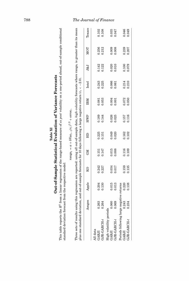
788 The Journal of Finance
Tab
leX
IO
ut-
of-S
amp
leS
tati
stic
alE
valu
atio
nof
Var
ian
ceF
orec
asts
Th
ista
ble
repo
rts
the
R2
from
ali
nea
rre
gres
sion
ofth
era
nge
-bas
edm
easu
reof
expo
stvo
lati
lity
ona
one-
peri
odah
ead,
out-
of-s
ampl
eco
ndi
tion
alst
anda
rdde
viat
ion
fore
cast
from
the
resp
ecti
vem
odel
:
ran
get=
a+
bVar
t−1(r
t)1/
2+
erro
r t.
Th
ree
sets
ofre
sult
su
sin
gth
isre
gres
sion
are
repo
rted
:usi
ng
allo
ut-
of-s
ampl
eda
ta,h
igh
-vol
atil
ity
fore
cast
sw
her
era
nge
tis
grea
ter
than
its
mea
npl
us
one
stan
dard
devi
atio
n,a
nd
out-
of-s
ampl
efo
reca
sts
for
10da
ysfo
llow
ing
ala
rge
neg
ativ
ere
turn
(rt<
−2.0
).
Am
gen
App
leK
OG
MH
DH
WP
IBM
Inte
lJ&
JM
OT
Tex
aco
All
data
GA
RJI
0.26
30.
204
0.24
20.
151
0.22
50.
189
0.08
10.
243
0.14
20.
256
0.10
2G
JR-G
AR
CH
-t0.
264
0.13
00.
227
0.14
70.
151
0.14
40.
053
0.22
50.
122
0.21
20.
108
Hig
hvo
lati
lity
peri
ods
GA
RJI
0.06
00.
015
0.03
40.
015
0.04
90.
026
0.00
40.
066
0.02
00.
009
0.03
5G
JR-G
AR
CH
-t0.
069
0.01
30.
017
0.00
80.
020
0.02
50.
001
0.06
10.
010
0.00
80.
047
Per
iods
foll
owin
gla
rge
neg
ativ
ere
turn
sG
AR
JI0.
243
0.22
00.
159
0.11
60.
162
0.15
70.
072
0.21
40.
100
0.23
90.
046
GJR
-GA
RC
H-t
0.23
40.
138
0.13
50.
109
0.10
20.
116
0.05
00.
210
0.07
90.
207
0.04
9
Individual Stock Returns 789
mixture of distributions, which allows the shape of the tails of the return distri-bution to change over time. Therefore, the more flexible GARJI model shouldbe able to capture dynamics in the tails of the return distribution, particularlyafter a large price move. In Section III.A.3, we illustrated the improved fore-casts of the GARJI model after the 1987 crash for IBM. This suggested that theaddition of jump dynamics plays an important role in improving forecasts aftera large negative move in the market. Again, the important question is whetherour richer specification also performs better for out-of-sample forecasts. To in-vestigate this for all firms, we consider another conditional regression eval-uating out-of-sample forecasts using data around large negative returns. Inparticular, we condition on the daily return being less than negative two per-cent and include the 10 days immediately following this downward move inthe market. The R2s from the regression (26) associated with the out-of-sampleforecasts for these episodes in our sample are reported in the bottom panel ofTable XI. As expected, the predictive ability of both models declines comparedto the top row which includes all of the data, but the GARJI specification con-tinues to provide superior forecasts compared to the GJR-GARCH-t alternativefor 10 out of 11 firms.
In summary, the results in the three panels of Table XI show that the GARJImodel produces superior forecasts relative to a benchmark GJR-GARCH-tmodel. These results include out-of-sample forecasts for average volatility,above average volatility, and the volatility just after large negative moves inthe stock price. These substantial improvements in the out-of-sample forecasts,relative to a popular benchmark model, should facilitate improved financialmanagement decisions.
V. Summary
In this paper we have developed a model of the components of the returndistribution implied by the impact of different types of news. We interpret theinnovation to returns, which is directly measurable from price data, as thenews impact from latent news innovations. The latent news process is pos-tulated to have two separate components, normal and unusual news events,which have different impacts on returns, expected volatility, and higher-ordermoments of the return distribution. Normal news innovations are assumed tocause smoothly evolving changes. The second component of the latent newsprocess causes infrequent large moves in returns which we label jumps. There-fore, the latent news process induces two separate components governing thedistribution of returns.
The volatility process is affected by both components driving returns. The con-ditional variance of the normal innovation captures the smooth autoregressivecomponent in volatility; whereas the conditional variance of the jump inno-vation captures unusual and often extreme price movements from significantinformation events. The intensity of the jump process is explicitly modeledas a serially correlated conditional Poisson process. This time-varying inten-sity affects volatility dynamics directly. In addition, previous jump innovations

790 The Journal of Finance
feed back into expected volatility through the GARCH component of condi-tional variance. Furthermore, normal and jump innovations have potentiallyasymmetric effects on volatility dynamics. This rich specification allows for con-ditional contemporaneous leverage effects and lagged leverage effects. Thesefeatures extend traditional models that combine GARCH and SV with jumps.
In summary, we find evidence of time dependence in jump intensities forboth individual stocks and indices using an autoregressive conditional jumpintensity parameterization; allow jump innovations to feed back to expectedvolatility; provide new results on asymmetric effects of return innovations onvolatility; and find evidence of a time-varying contemporaneous leverage ef-fect. These novel features allow jumps to have different impacts, feed backs,and decay rates as compared to normal innovations allowing the model to per-form better around crash periods and other events in the tail of the distribu-tion. The structure of our model is such that the mixture of components canadapt flexibly to capture different features of the conditional distribution ofreturns. Importantly, our GARCH-jump mixture model also provides superiorout-of-sample conditional variance forecasts relative to a benchmark asymmet-ric GARCH model with fat-tailed innovations. These superior out-of-sampleforecasts should result in improvements in financial management.
Finally, the process governing the arrival of jumps may be heterogeneouswith respect to the type of news. For example, some macro and firm-specific an-nouncement dates are known ex ante and may result in deterministic volatilitythat is identified as a jump. In other words, jump dynamics may differ acrossdifferent types of news events. However, the infrequent occurrence of jumpsmakes this identification of different jump dynamics a challenging area forfuture study.
Appendix
For notational convenience let E[· | �t−1] = Et−1. The conditional intensitycan be rewritten as
λt = λ0
∞∑i=0
ρi + γ
∞∑i=1
ρi−1ξt−i + limk→∞
ρkλt−k . (A1)
Now for |ρ| < 1 and, limk→∞ρkEλt−k = 0,
Eλt = λ0
1 − ρ. (A2)
The further restrictions of ρ ≥ γ ≥ 0, and λ0 > 0 ensures that λt > 0 for all t.For the GARCH-jump model with the following restrictions, αj = αa = αa, j = 0,and with the GARCH function parameterized as
σ 2t = ω + αε2
t−1 + βσ 2t−1, (A3)
Individual Stock Returns 791
the unconditional variance is composed of the two components,
E(rt − µ)2 = E(ε2
1,t + 2ε1,tε2,t + ε22,t
)(A4)
= Eσ 2t + Eε2
2,t . (A5)
To solve for Eε22,t, first note that Vart−1(ε2,t) = Et−1ε
22,t = (θ2 + δ2)λt , since by
construction Et−1ε2,t = 0. Therefore,
Eε22,t = E Et−1ε
22,t = (θ2 + δ2)E(λt) (A6)
= (θ2 + δ2)λ0
1 − ρ. (A7)
To find Eσ 2t we have
Et−2σ2t = ω + (α + β)σ 2
t−1 + αEt−2ε22,t−1, (A8)
or in general,
Et−kσ 2t = ω(1 + (α + β) + · · · + (α + β)k−2) + (α + β)k−1σ 2
t−k+1 (A9)
+ α(Et−kε2
2,t−1 + (α + β)Et−kε22,t−2 + · · ·
+ (α + β)k−2 Et−kε22,t−k+1
). (A10)
Under the above conditions that ensure Eλt exists and α + β < 1,
limk→∞
Et−kσ 2t = ω
(1 − α − β)+ α
(1 − α − β)(θ2 + δ2)
λ0
1 − ρ(A11)
and therefore,
Var(rt) = ω
(1 − α − β)+ α(θ2 + δ2)
(1 − α − β)λ0
(1 − ρ)+ (θ2 + δ2)
λ0
(1 − ρ). (A12)
REFERENCESAndersen, Torben G., 1996, Return volatility and trading volume: An information flow interpreta-
tion of stochastic volatility, Journal of Finance 51, 169–204.Andersen, Torben G., Luca Benzoni, and Jesper Lund, 2002, An empirical investigation of
continuous-time equity return models, Journal of Finance 62, 1239–1284.Andersen, Torben G., and Tim Bollerslev, 1998a, Answering the skeptics: Yes, standard volatility
models do provide accurate forecasts, International Economic Review 39, 885–905.Andersen, Torben G., and Tim Bollerslev, 1998b, Deutsche mark-dollar volatility: Intraday activity
patterns, macroeconomic announcements, and longer run dependencies, Journal of Finance 53,219–265.

792 The Journal of Finance
Baillie, Richard T., and Yun Han, 2001, Comment on testing target-zone models using efficientmethod of moments, Journal of Business and Economic Statistics 19, 273–276.
Ball, Clifford A., and Walter N. Torous, 1983, A simplified jump process for common stock returns,Journal of Financial and Quantitative Analysis 18, 53–65.
Bates, David S., 1991, The crash of ’87: Was it expected? The evidence from the options markets,Journal of Finance 46, 1009–1044.
Bates, David S., 2000, Post-’87 crash fears in the S&P 500 futures option market, Journal ofEconometrics 94, 181–238.
Bates, David S., 2001, The market for crash risk, Working Paper, University of Iowa, FinanceDepartment.
Bates, David S., and Roger Craine, 1999, Valuing the futures market clearinghouse’s default expo-sure during the 1987 crash, Journal of Money, Credit, and Banking 31, 248–272.
Bekaert, Geert, and Stephen F. Gray, 1998, Target zones and exchange rates: An empirical inves-tigation, Journal of International Economics 45, 1–35.
Campbell, John Y., and Ludger Hentschel, 1992, No news is good news: An asymmetric model ofchanging volatility in stock returns, Journal of Financial Economics 31, 281–318.
Campbell, John Y., Martin Lettau, Burton G. Malkiel, and Yexiao Xu, 2001, Have individual stocksbecome more volatile? An empirical exploration of idiosyncratic risk, Journal of Finance 56,1–43.
Chan, Wing H., and John M. Maheu, 2002, Conditional jump dynamics in stock market returns,Journal of Business & Economic Statistics 20, 377–389.
Chernov, Mikhail, A. Ronald Gallant, Eric Ghysels, and George Tauchen, 2003, Alternative modelsfor stock price dynamics, Journal of Econometrics, forthcoming.
Cho, Young-Hye H., and Robert F. Engle, 1999, Time-varying betas and asymmetric effects of news:Empirical analysis of blue chip stocks, NBER Working Paper 7330.
Clark, Peter K., 1973, A subordinated stochastic process model with finite variance for speculativeprices, Econometrica 41, 135–155.
Das, Sanjiv R., 2002, The surprise element: Jumps in interest rate, Journal of Econometrics 106, 27–65.
Das, Sanjiv R., and Rangarajan K. Sundaram, 1997, Taming the skew: Higher-order moments inmodeling asset price processes in finance, NBER Working Paper 5976.
Duffee, Greg R., 1995, Stock returns and volatility: A firm-level analysis, Journal of FinancialEconomics 37, 399–420.
Engle, Robert F., and Chaudhury Mustafa, 1992, Implied ARCH models from options prices, Journalof Econometrics 52, 289–311.
Engle, Robert F., and Victor K. Ng, 1993, Measuring and testing the impact of news on volatility,Journal of Finance 48, 1749–1778.
Eraker, Bjorn, Michael S., Johannes, and Nicholas G. Polson, 2003, The impact of jumps in volatilityand returns, Journal of Finance 58, 1269–1300.
Feinstone, Laura J., 1987, Minute by minute: Efficiency, normality, and randomness in intra-dailyasset prices, Journal of Applied Econometrics 2, 193–214.
Glosten, Lawrence, and Paul Milgrom, 1985, Bid, ask, and transaction prices in a specialist marketwith heterogenously informed traders, Journal of Financial Economics 14, 71–100.
Glosten, Lawrence R., Ravi Jagannathan, and David E. Runkle, 1993, On the relation between theexpected value and the volatility of the nominal excess return on stocks, Journal of Finance48, 1779–1801.
Hansen, Bruce E., 1994, Autoregressive conditional density estimation, International EconomicReview 35, 705–730.
Harvey, Campbell R., and Akhtar Siddique, 1999, Autoregressive conditional skewness, Journalof Financial and Quantitave Analysis 34, 465–487.
Johannes, Michael, Rohit Kumar, and Nicholas G. Polson, 1999, State dependent jump models:How do U.S. equity indices jump?, Working Paper, Graduate School of Business, University ofChicago.
Jorion, Philippe, 1988, On jump processes in the foreign exchange and stock markets, Review ofFinancial Studies 1, 427–445.

Individual Stock Returns 793
Neely, Christopher J., 1999, Target zones and conditional volatilty: The role of realignments, Jour-nal of Empirical Finance 6, 177–192.
Nelson, Daniel B., 1991, Conditional heteroskedasticity in asset returns: A new approach, Econo-metrica 59, 347–370.
Nieuwland, Frederick, Willem Vershchoor, and Christian Wolff, 1994, Stochastic trends and jumpsin EMS exchange rates, Journal of International Money and Finance 13, 699–727.
Oomen, Roel C.A., 2002, Statistical models for high frequency security prices, Working Paper,Warwick Business School, University of Warwick.
Pan, Jun, 1997, Stochastic volatility with resets at jumps, Working Paper, Graduate School ofBusiness, Stanford University.
Pan, Jun, 2002, The jump-risk premia implicit in options: Evidence from an integrated time-seriesstudy, Journal of Financial Economics 63, 3–50.
Parkinson, Michael, 1980, The extreme value method for estimating the variance of the rate ofreturn, Journal of Business 53, 61–65.
Perez-Quiros, Gabriel, and Allan Timmermann, 2001, Business cycle asymmetries in stock returns:Evidence from higher order moments and conditional densities, Journal of Econometrics 103,259–306.
Premaratne, Gamini, and Anil K. Bera, 2001, Modeling asymmetry and excess kurtosis in stockreturn data, Working Paper, Department of Economics, University of Illinois.
Press, S. James, 1967, A compound events model for security prices, Journal of Business 40, 317–335.
Ross, Stephen A, 1989, Information and volatility: The no-arbitrage martingale approach to timingand resolution irrelevancy, Journal of Finance 44, 1–17.
Schwert, G. William, 1990, Stock market volatility and the crash of ’87, Review of Financial Studies3, 77–102.
Tauchen, George E., and Michael Pitts, 1983, The price variability-volume relationship on specu-lative markets, Econometrica 51, 485–505.
Vlaar, Peter J.G., and Franz C. Palm, 1993, The message in weekly exchange rates in the Euro-pean monetary system: Mean reversion, conditional heteroscedasticity, and jumps, Journal ofBusiness & Economic Statistics 11, 351–360.
Yu, Jun, 2003, Empirical characteristic function estimation and its applications, EconometricReviews, forthcoming.