Dedicated to: Hediyeh

List of Papers

This thesis is based on the following papers, which are referred to in the text by their Roman numerals.

I. Beiki, M., and Pedersen, L. B. (2010), Eigenvector analysis of

gravity gradient tensor to locate geologic bodies. Geophysics, 75(6): I37-I49.

II. Beiki, M., Pedersen, L. B., and Nazi, H. (2011), Interpretation of aeromagnetic data using eigenvector analysis of pseudo-gravity gradient tensor. Submitted to Geophysics, accepted.

III. Beiki, M. (2010), Analytic signals of gravity gradient tensor and their application to estimate source location. Geophysics, 75(6): I59-I74.

IV. Beiki, M., and Pedersen, L. B. (2011), Deconvolution of grav-ity gradient tensor data using infinite dike and geological con-tact models. Submitted to Geophysics, under review.

Reprints were made with permission from the respective publishers. Additional articles written during my PhD studies but not included in this thesis are: Beiki, M., and Pedersen, L. B. (2011), Comment on ‘’Depth estimation

of simple causative sources from gravity gradient tensor invariants and vertical component’’ by B. Oruç. Submitted to Pure and Applied Geo-physics, accepted.

Beiki, M., Bastani, M., and Pedersen, L. B. (2010), Leveling HEM and aeromagnetic data using differential polynomial fitting. Geophysics, 75(1): L13-L23.

Contents

1. Introduction ............................................................................................. 13 1.1 Motivation and general objective...................................................... 13 1.2 Structure of the thesis........................................................................ 14

2. Potential field theory ............................................................................... 15 2.1 Potential field .................................................................................... 15

2.1.1 Green’s identities....................................................................... 15 2.2 Gravity field ...................................................................................... 18

2.2.1 Three-dimensional gravity field ................................................ 20 2.2.2 Two-dimensional gravity field .................................................. 20 2.2.3 Regional gravity field and gravity corrections .......................... 21 2.2.4 Gravity gradient tensor.............................................................. 21

2.3 Magnetic field ................................................................................... 24 2.3.1 Three-dimensional magnetic field............................................. 26 2.3.2 Two-dimensional magnetic field............................................... 26 2.3.3 Geomagnetic field ..................................................................... 27

3. Airborne gravity and magnetic instruments ............................................ 29 3.1 Airborne gravimetry.......................................................................... 29 3.2 Airborne gravity gradiometry ........................................................... 30 3.3 Aeromagnetic surveys....................................................................... 31

4. Source parameter estimation techniques ................................................. 33 4.1 Werner deconvolution technique ...................................................... 33 4.2 Naudy method................................................................................... 34 4.3 Analytic signal techniques ................................................................ 35 4.4 Euler deconvolution technique.......................................................... 35 4.5 Local wavenumber methods ............................................................. 38 4.6 Equivalent source techniques............................................................ 38 4.7 Statistical methods ............................................................................ 39

5. Case studies ............................................................................................. 41 5.1 The Vredefort impact structure, South Africa .................................. 41

5.1.1 The impact structure within the Witwatersrand basin ............... 41 5.1.2 The Vredefort dome or central part of the impact structure ...... 42 5.1.3 AGG data from the Vredefort dome.......................................... 43

5.2 The Särna area, west central Sweden................................................ 47 5.2.1 Aeromagnetic data from the Särna area .................................... 47

6. Summary of papers.................................................................................. 49 6.1 Paper I: Eigenvector analysis of GGT to locate geologic bodies...... 49

6.1.1 Summary ................................................................................... 49 6.1.2 Conclusions ............................................................................... 50 6.1.3 Contribution .............................................................................. 51

6.2 Paper II: Interpretation of aeromagnetic data using eigenvector analysis of PGGT.................................................................................... 51

6.2.1 Summary ................................................................................... 51 6.2.2 Conclusions ............................................................................... 52 6.2.3 Contribution .............................................................................. 52

6.3 Paper III: Analytic signals of GGT and their application to estimate source location ........................................................................................ 53

6.3.1 Summary ................................................................................... 53 6.3.2 Conclusions ............................................................................... 54 6.3.3 Contribution .............................................................................. 55

6.4 Paper IV: Deconvolution of GGT data using infinite dike and geological contact models....................................................................... 55

6.4.1 Summary ................................................................................... 55 6.4.2 Conclusions ............................................................................... 56 6.4.3 Contribution .............................................................................. 57

7. Discussion and conclusions ..................................................................... 59 7.1 Discussion......................................................................................... 59

7.1.1 Application of sliding windows in the source parameter estimation techniques ......................................................................... 59 7.1.2 Discrimination of solutions and geological constraints............. 60 7.1.3 Improvement of results using complementary methods............ 60

7.2 General conclusions .......................................................................... 61 7.3 Future developments ......................................................................... 62

8. Summary in Swedish ............................................................................... 63 8.1 Egenvektoranalys av GGT- och PGGT- data (artiklarna I och II)... 63 8.2 Analytiska signaler av GGT för uppskattning av djup till störkroppar (artikel III) ........................................................................... 63 8.3 Dekonvolution av GGT-data med hjälp av modeller för oändliga geologiska gångar och kontakter (artikel IV) ......................................... 64

9. Acknowledgements ................................................................................. 65

A. Additional notes on impact structures .................................................... 67 A.1 Impact craters................................................................................... 67 A.2 Impact cratering ............................................................................... 67

A.2.1 Contact and compression.......................................................... 67 A.2.2 Excavation ................................................................................ 68 A.2.3 Modification ............................................................................. 68

A.3 Morphology of impact craters.......................................................... 70

A.3.1 Simple craters ........................................................................... 70 A.3.2 Complex craters........................................................................ 70 A.3.3 Multi-ring craters...................................................................... 71

A.4 Gravity signature of impact craters .................................................. 72

References ................................................................................................... 73

Abbreviations

2D Two-dimensional 3D Three-dimensional AGG Airborne Gravity Gradiometry GGT Gravity Gradient Tensor LPI Lunar and Planetary Institute MGT Magnetic Gradient Tensor PDF Planar Deformation Features PGGT Pseudo-Gravity Gradient Tensor TIB Trans-Scandinavian Igneous Belt

13

1. Introduction

1.1 Motivation and general objective Studies of the Earth’s gravity and magnetic fields are examples of modern applications of classical Newtonian physics. Gravity and magnetic fields are routinely measured in mineral exploration, hydrocarbon exploration, crustal studies, environmental engineering and exploration of geothermal resources. Gravity and magnetic surveys are carried out using ground, airborne, ship-borne, satellite or borehole measurement systems. Among those, airborne is the most popular type of survey because of its cost-efficiency and rapid cov-erage of large areas.

Airborne magnetic is the oldest airborne geophysical technique which has been in use since 1943. The first application of airborne magnetic surveys was for detecting submarines in World War II. By advancements of instru-mentations and developing navigation systems, airborne gravity measure-ments became feasible in the early 1990s.

Gradients of gravity and magnetic fields are much more sensitive to short wavelength anomalies than gravity and magnetic fields. In the last two dec-ades, airborne and shipborne gravity gradiometers use developed for routine measurements and introduced to industry. At the time of writing this thesis, airborne magnetic gradiometry instruments are still under development. However, it is anticipated that in the near future, airborne magnetic gradi-ometers will be commercially available.

The gradient tensors of gravity and magnetic fields contain the first order derivatives of the gravity and magnetic vectors in three orthogonal direc-tions. Mathematical properties of gravity and magnetic gradient tensors sug-gest new processing and interpretation techniques. In recent years, several new techniques for interpretation of GGT data have been introduced in the literature (e.g. Pedersen and Rasmussen, 1990; Vasco and Taylor, 1991; Edwards et al., 1997; Routh et al., 2001; Zhdanov et al., 2004; Droujinine et al., 2007; While et al., 2006; Mikhailov et al., 2007; Pajot et al., 2008; While et al., 2009; Beiki and Pedersen, 2010; Beiki, 2010). However, both processing and interpretation of GGT data are still challenging and requires further development.

The general objective of this thesis is to develop new techniques for processing and interpretation of airborne gravity gradient tensor data. In particular, this thesis includes four papers. In paper I, a new interpretation technique is introduced for GGT data based on Pedersen and Rasmussen

14

(1990). In paper II, it is shown that the same mathematical properties of GGT data can be used for interpretation of pseudo-gravity gradient tensor (PGGT) derived from magnetic field data assuming that the magnetization direction is known. Paper III describes that the analytic signal concept can be extended to 3D GGT. It is also shown that the amplitudes of the analytic signals satisfy Euler’s homogeneity equation and they can be used to esti-mate source location. Paper IV contains a new deconvolution approach for GGT data using infinite dike and geological contact models. The applica-tions of introduced methods are demonstrated on an airborne GGT data set from the Vredefort impact structure, South Africa and an aeromagnetic data set from the Särna area, west central Sweden.

1.2 Structure of the thesis Before presenting the developed methods for interpretation of GGT and PGGT data, a brief description of potential field theory is provided in chap-ter 2 to explain theoretical basis of the thesis. Then, I shortly describe the commercially available airborne gravity and gradiometry instruments as well as different types of magnetometers adopted for airborne measurements in chapter 3. The source estimation techniques which are widely adopted for interpretation of gravity and magnetic data are described in chapter 4. In particular, those have capabilities to be employed for interpretation of GGT data are discussed in more details. Geological settings of the Vredefort im-pact structure, South Africa and the Särna area, west central Sweden are outlined in chapter 5. In order to have a better understanding of impact structures, additional notes on the structural geology of the impact structures are provided in Appendix A. The principles of the developed methods are summarized in chapter 6. Chapter 7 contains discussion and conclusions of the developed methods and their applications to the real data examples and finally a short summary of the thesis in Swedish is given in chapter 8.

15

2. Potential field theory

2.1 Potential field A field can be defined as a function that might be a scalar or a vector which holds space and time variations of a physical quantity. Temperature distribu-tion throughout space and magnetic field are examples of scalar and vector fields, respectively. A vector field F is said to be conservative if the work required to move a particle from one point to another is independent of the path connecting the two points. When F is conservative it is called a poten-tial field if it is related to the scalar potential Ø such that F= Ø. This im-plies that potential fields are irrotational, ×F=0. The potential Ø is a har-monic function and satisfies Laplace’s equation 2Ø=0 outside the source of the potential field F. The solutions to Laplace’s equation are known as harmonic functions.

2.1.1 Green’s identities Like any differential equation, a complete solution of Laplace’s equation is obtained only by application of boundary conditions. Some fundamental theorems and identities are derived from vector calculus and Laplace’s equation to study the existence and uniqueness of solutions to these bound-ary value problems.

Green’s first identity is derived from the divergence theorem applied to the vector field F= Ø where Ø and are scalar functions defined on region R and continuously differentiable to second and first orders, respec-tively. The region R is bounded by the surface boundary S with outward normal n :

SRR

2 ØØØ ds

ndvdv . (2.1)

Green’s second identity is obtained by interchanging Ø and in equation 2.1 and subtracting the new equation from equation 2.1,

SR

22 )Ø

Ø()ØØ( dsnn

dv . (2.2)

16

Now, by choosing =r

1 in Green’s second identity (equation 2.2), where r

is the distance between integration (point Q) and observation (point P) in the region R, the potential Ø at the observation point is

SSR

2

)1

(Ø4

1Ø1

4

1

r

Ø

4

1)P( Ø ds

rnds

nrdv . (2.3)

Equation 2.3 is known as Green’s third identity. Kellog (1953) and Blakely (1995) present a detail proof of the Green’s identities as well as theorems derived from them.

Several interesting theorems are derived from Green’s identities to prove the uniqueness of solutions to Laplace’s equation. Here, I briefly describe some important theorems which are useful to understand the potential field theory in general. One of the important theorems (Green’s equivalent layer) derived from Green’s identities remains to be discussed in the next section after describing the gravity field.

Theorem 1. If = 1 and Ø is harmonic, then 2Ø = 0 and = 0. Therefore, from equation 2.1 we have

0Ø

Sds

n (2.4)

while on the surface of the region

nF ˆØ

n. (2.5)

By substituting 2.5 into equation 2.4 and applying the divergence theorem we get

0R

dvF . (2.6)

The condition .F = 0 within the region is sufficient to conclude that the region is free of any sources.

Theorem 2. If Ø is harmonic and continuously differentiable in region R surrounded by surface S, and if Ø vanishes at surface S, it vanishes at all points located within the region R.

Theorem 3 (Stokes’ theorem). If Ø is harmonic and continuously differ-entiable in closed region R, then Ø can uniquely be determined in the region by its values on the boundary surface S.

Theorem 4. If Ø and are both harmonic and =1, from Green’s second identity (equation 2.2) we get the same result as theorem 1:

0S

dsnF . (2.7)

17

In words, the flux of a conservative field through a closed surface, S is equal to zero.

Theorem 5. If Ø is harmonic, then by substituting 2Ø=0 in equation 2.3, we get

S)

1(Ø

Ø1

4

1(P)Ø ds

rnnr (2.8)

which means that having the values of a harmonic function Ø and its normal derivatives on a closed surface S, one can calculate Ø at any point inside the region R enclosed by S. Equation 2.8 is simplified by eliminating the term

containingn

Øwhich leads to derivation of a practical formula. Assuming

that Ø and are both harmonic, the left side of equation 2.2 (Green’s sec-ond identity) vanishes. By adding the resulting equation to equation 2.8, we have

S

Ø)

1()

1(Ø

4

1(P)Ø ds

nrrn. (2.9)

With =r

1at surface S, we get

S)

1(Ø

4

1(P)Ø ds

rn. (2.10)

Assuming a half-space region (Figure 2.1) where Ø is harmonic throughout, if we choose point P such that it is located below the surface z=0 and has a

distance rr to point Q, by letting =r

1

S)

11(Ø

4

1(P)Ø ds

rrn. (2.11)

Equation 2.11 can be written as

ddr

zzyx

3

0) , ,(Ø

2)- , ,(Ø (2.12)

where 222 )()( zyxr . Equation 2.12 is called upward continua-

tion operation and states that the potential Ø can be calculated at any point above the surface on which the potential is measured (Blakely, 1995). Up-ward continuation is one of the most practical implications of Green’s iden-tities.

18

Figure 2.1. A half-space region above surface z = 0 where Ø is harmonic.

2.2 Gravity field Newton’s law of universal gravitation states that any two point masses in the universe exert a gravitational force of attraction on each other which is di-rectly proportional to the product of their masses and inversely proportional to the square of the distance between them (Figure 2.2).

Figure 2.2. The illustration of the Newton’s law of universal gravitation.

Assuming that m is a unit mass then the gravitational attraction caused by point mass m0 at P is

rg ˆ)P(20

r

m (2.13)

where = 6.67×10-11 m3/kg.s2 (SI system) is gravitational constant and unit

vector kjir ˆ)(ˆ)(ˆ)(1ˆ

000 zzyyxxr

is directed from the mass m0

toward the unit mass m. Gravitational attraction is a conservative field and it is related to the gravitational potential U through

19

U)P(g (2.14)

with

r

m)P(U . (2.15)

Note: Mass and potential are related through Poisson’s equation

4U2 (2.16)

and Laplace’s equation 02 U is only a special case of Poisson’s equation valid in source free regions.

Theorem 6. If S is a closed equipotential surface caused by a 3D density distribution and R is the region surrounded by S (Figure 2.3), Green’s second identity (equation 2.2) can be simplified to

Ss

R

2 Ø1)

1(Ø

Øds

nrrndv

r (2.17)

where Ø is the potential of the mass, r denotes the distance from point P

located outside the region, = r

1 and Øs is the potential at the equipotential

surface. By substituting equations 2.4 and 2.16 into equation 2.17, Green’s equivalent layer is given as

SR

Ø1

4

1ds

nrdv

r. (2.18)

In words, a gravitational potential caused by a three-dimensional source distribution with arbitrary shape is equivalent to the potential produced by a surface density distribution over any of its equipotential surfaces (Ramsey, 1940).

20

Figure 2.3. Equipotential surface S caused by a point source. S is a closed surface but to have a better illustration it is cut off from sides.

2.2.1 Three-dimensional gravity field Considering a three-dimensional mass of arbitrary shape, the potential and gravity field at a point outside the mass can be calculated by superposition of small elements. Hence, the potential of the total mass m is

vdR

rrrr )(

)(U (2.19)

where r and r’ denote observation and integration points, respectively. Con-sequently, the gravity vector is given as

vdR

rrrrrg ˆ)(

)( 2 . (2.20)

The potential of a solid sphere at points located outside the source is equal to the potential caused by a point source located at the center of the sphere with an identical total mass m.

2.2.2 Two-dimensional gravity field In the case of a two-dimensional mass distribution striking in the y-direction with a cross section of arbitrary shape in the xz-plane, the potential and gravity vector are, respectively:

21

zdxdx z

1ln)(2)(U

rrrr (2.21)

and

zdxdrrr

rrg ˆ)(2)(

x z

. (2.22)

A theoretical example for a 2D source is an infinite horizontal cylinder. Similar to the point mass described earlier, the potential of a solid horizontal cylinder at points located outside the source is equal to an infinite number of point sources with a mass per unit length m lying next to each other located on the axis of the cylinder. Then, the potential and gravity vector associated with an infinite horizontal cylinder is given as

rm ln 2)(U r (2.23)

and

rrg ˆ2)(

r

m. (2.24)

2.2.3 Regional gravity field and gravity corrections The vertical component of the gravity vector, gz, was first measured by Gali-leo Galilei about 1589. In honor of Galilei, the unit of gravity field is called Gal=0.01 m/s2. However, because of small variations of gravity fields caused by local masses and the sensitivity of gravimeters used in the field measurements, mGal=10-3 Gal is adopted as unit of gravity field (Telford et al., 1990).

In order to interpret short wavelength gravity anomalies caused by local masses with positive or negative density contrasts, a key step should be car-ried out to separate regional field from the anomaly caused by the target source prior to analysis of measured gravity field. The separation procedure involves a series of corrections to the measured gravity field. Blakely (1995) describes that the measured gravity field contains different effects of lati-tude, moving platforms, elevation above sea level, topography of the sur-rounding terrain and earth tides which require free-air, Bouguer, terrain, tidal, Eötvös and isostatic corrections. Readers are referred to text books e.g. Telford et al. (1990) and Blakely (1995) for details about gravity data cor-rections.

2.2.4 Gravity gradient tensor The history of gravity gradiometry goes back to 1886 when Lorand Eötvös, the Hungarian scientist, introduced his first torsion balance gradiometer to

22

the oil industry (Bell and Hansen, 1998). After Eötvös, the unit of gravity gradients is called Eötvös which is equal to 10-4 mGal/m. In the 1970’s new systems were developed to measure gradients of gravity vector components mainly for military purposes (Bell et al., 1997). About three decades later, new gravity gradiometry systems were introduced to industry for hydrocar-bon exploration, mineral exploration, structural geology, environmental engineering and geoid computations in geodesy.

As was described, the gravity vector is the gradient of the gravitational potential Ø in three Cartesian directions. Similarly, the next order of spatial derivatives yields a second-rank tensor:

zzyzxz

yzyyxy

xzxyxx

ggg

ggg

ggg

z

U

zy

U

zx

U

zy

U

y

U

yx

U

zx

U

yx

U

x

U

2

2

2

222

222

222

g .

(2.25)

Outside the source region, U satisfies Laplace’s equation, and hence the trace of the tensor is equal to zero. Since is symmetric, it only contains five independent components and can be diagonalized as:

VT V= (2.26)

where V=[v1 v2 v3] and

3

2

1

00

00

00

contain eigenvectors and eigen-

values, respectively. Physically, with the origin of the coordinate system at any observation point, equation 2.26 means that one can find a new coordi-nate system with axes along the eigenvectors in which the gradient tensor is on diagonal form. Pedersen and Rasmussen (1990) introduced the following three invariants:

I0 = Trace ( ) = 1+ 2+ 3 = 0, (2.27)

I1 = 11 22 + 22 33 + 11 33 – 122 – 23

2 – 132 = 1 2+ 2 3+ 1 3

(2.28) and

I2 = det ( ) = 1 2 3 . (2.29)

23

They showed that the invariant ratio 3

1

2

2

4

27

I

II lies between zero and unity

for any potential field. When the causative body as seen from the observa-tion point looks more and more 3D like, then I increases and eventually approaches unity and

321

32

22. (2.30)

With 2D geometry of sources striking in the y direction, the number of non-zero GGT components reduces to four with two independent elements

zzxz

xzxx

gg

gg

z

U

zx

U

zx

U

x

U

2

22

2

2

2

g . (2.31)

Then for a strict 2D case, I is equal to zero for all measurement points and

02

31 . (2.32)

For a quasi 2D body, the projection of the third eigenvector correspond-ing to the minimum eigenvalue onto the horizontal plane is directed along the strike of the body while the eigenvector corresponding to the intermedi-ate eigenvalue is along the maximum gradient of the field.

The potential U, the gravity vector and the GGT components correspond-ing to the theoretical examples of a mass point source and a mass line source striking in y direction are listed in Table 2.1 when x= x0 – x, y= y0 – y and

z= z0 – z. In reality, many of 2D geological structures can be approximated by infi-

nite dike and geological contact models which make them more practical than the infinite horizontal cylinder model for interpretation of magnetic and gravity field data (e.g., Nabighian, 1972 and 1974; Hsu et al., 1998; Bastani and Pedersen, 2001; Beiki and Pedersen, 2010). Telford et al. (1990) and Stanley and Green (1976) have shown expressions for the gravity gradients gxz and gzz caused by infinite dike and geological contact models, respec-tively. Application of these models in interpretation of GGT data is demon-strated in paper IV.

24

Table 2.1. Gravity and GGT components of mass point and mass line sources.

2.3 Magnetic field The word magnetism comes from the Greek ancient city of magnesia which was known because of certain magnetic rocks in the vicinity of this city (Roy, 2008). Oersted (1819) was the first to observe the connection between the flow of electric current through a wire and the generated magnetic field. One year later, Biot and Savart described the relation between the magnetic induction B generated by an electric current. In the same year, Ampere pro-posed his force law describing that there is an effective force between two parallel wires carrying an electric current.

Magnetic field is always a solenoidal field even within magnetic media

.B = 0. (2.33)

This is the most significant difference between magnetostatic field and other fields like electrostatic field, gravity field, heat flow field etc, in which sat-isfy Laplace’s equation only in source free regions. Unlike the gravity field, magnetostatic field is a rotational field and

×B=4 CmIt (2.34)

Point source Line source

U rm rm ln

gx 3rxm 2rxm

gy 3rym –

gz 3rzm 2rzm

gxx 5223 rrxm 4222 rrxm

gxy 53 ryxm –

gxz 53 rzxm 42 rzxm

gyy 5223 rrym –

gyz 53 rzym –

gzz 5223 rrzm 4222 rrzm

25

where Cm=10-7 Henry/m is a proportionality constant and It is current source. Assuming that there is no current source in the region, B is irrotational and it can be defined as the gradient of a scalar potential V

B = V. (2.35)

This approximation is valid only outside magnetic media where electric currents are negligible.

The potential of a magnetic dipole observed at point P is given as (Blake-ly, 1995)

rr

1.C

ˆ.CV(P) m2m PMrM

(2.36)

where sˆInM is the magnetic dipole moment with unit of ampere.m2 in SI system, I is the current in ampere, n is a unit normal vector and s is the area of the loop in m2. Poisson’s equation for magnetic scalar potential can be written as (Roy, 2008)

M4V2 . (2.37)

The magnetic induction of a magnetic dipole is acquired by substituting equation 2.36 into equation 2.35:

0;ˆˆ)ˆˆ(3CB3m r

r

m M-rrM . (2.38)

The magnetization of a volume V in ampere/m is defined as sum of indi-vidual dipole moments divided by the volume V (Blakely, 1995). In the SI system, the difference between magnetic induction normalized to the mag-netic permeability of free space 0 and magnetization is called magnetic field intensity

MBH0

(2.39)

where 0 is the magnetic permeability of free space in Henry/m. Note: H and B in the cgs system are identical outside the source region

whereas in the SI system they have the same direction but different magni-tudes and dimensions. Their units in the SI system are ampere/m and we-ber/m2=Tesla, respectively. For more details about units and their conver-sions, readers are referred to Blakely (1995).

The induced magnetization of rocks in the direction of an inducing field H is

M= H (2.40)

where is the dimensionless magnetic susceptibility. The total magnetiza-tion of rocks, M is equal to the sum of induced and remanent magnetizations

26

and the ratio between their magnitudes is expressed by Koenigsberger ratio

i

r

M

MQ where Mi and Mr are induced and remanent magnetizations, re-

spectively.

2.3.1 Three-dimensional magnetic field A uniformly magnetized volume of magnetic materials can be considered as a single dipole and subsequently its potential and magnetic induction at point P are (Blakely, 1995):

vdR

rrrMr r

1)(C)V( m (2.41)

and

vdR

rrrMrrB rrr

1)(C)V()( m (2.42)

where r and r’ are observation and integration points, respectively. The magnetic potential corresponding to a uniformly magnetized sphere is equal to the potential of a dipole (equation 2.36) located at the center of the sphere with a magnetic moment equal to the magnetization multiplied by the vol-ume of the sphere.

2.3.2 Two-dimensional magnetic field In analogy with gravitational potential, the magnetic potential corresponding to a two-dimensional source striking in the y direction with arbitrary cross section in xz-plane is given as

zdxdx z

m

ˆ)(C2)(V

rrrrMr . (2.43)

Consequently applying B = V provides:

zdxdx z

mˆˆ)ˆˆ(2

)(C2(P) M-rrM

rrrMB . (2.44)

The potential and magnetic field of an infinite horizontal cylinder with uni-form magnetization can be written as

rrr m rˆ

C2)(V m (2.45)

and

27

m-rrmrr

rB ˆˆ)ˆˆ(2C2

)( 2mm

(2.46)

where m is dipole moment per unit length.

2.3.3 Geomagnetic field William Gilbert (1540–1630) was the first to explain the existence of the earth magnetic field. He described that the field observed at the earth surface originates from the interior of the earth. Now using the satellites and space probe data it is understood that a significant part of the earth magnetic field has internal origin and only a small portion of the observed field (about 1%) is of extra terrestrial origin (Roy, 2008).

The magnetic field B can be described in terms of its deviation from the horizontal plane and the angle between its projection onto the horizontal plane (magnetic north) and the geographic north which are called inclination and declination of the field, respectively (Figure 2.4). The inclination and declination can be found from the horizontal and vertical components of the magnetic field such that

2y

2x

y1-

2y

2x

z1-

BB

BsinD

BB

BtanI

. (2.47)

The International Geomagnetic Reference Field (IGRF) is a mathematical model of the Earth’s main magnetic field which is widely used in studies of the Earth’s deep interior, the crust and ionosphere and magnetosphere. The IGRF is a result of an international collaboration between institutes and agencies responsible for collecting and publishing magnetic field data. The IGRF incorporates data from permanent observations at several base stations around the world as well as from land, airborne, marine and satellite sur-veys. The IGRF model is updated every five years by International Associa-tion of Geomagnetism and Aeronomy (IAGA) due to the time dependent variations of the geomagnetic field. Short period variations of the magnetic field are mainly caused by electric currents in the ionosphere. They are sub-divided into different scales of solar diurnal variations with a period of 24 hours, lunar variations with a period of 25 hours and magnetic storms caused by sunspot activities. In addition there are longer period variations called geomagnetic secular variations which are due to the variation in fluid outer core of the earth (Telford et al., 1990).

28

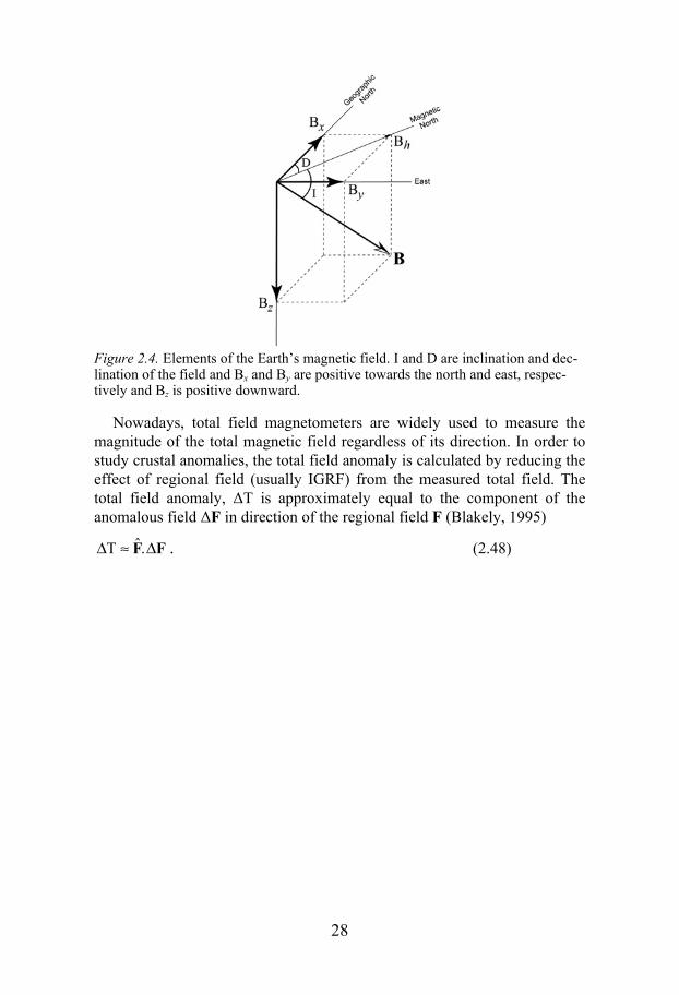
Figure 2.4. Elements of the Earth’s magnetic field. I and D are inclination and dec-lination of the field and Bx and By are positive towards the north and east, respec-tively and Bz is positive downward.

Nowadays, total field magnetometers are widely used to measure the magnitude of the total magnetic field regardless of its direction. In order to study crustal anomalies, the total field anomaly is calculated by reducing the effect of regional field (usually IGRF) from the measured total field. The total field anomaly, T is approximately equal to the component of the anomalous field F in direction of the regional field F (Blakely, 1995)

FF.ˆT . (2.48)

29

3. Airborne gravity and magnetic instruments

In recent years due to the advancements of methodologies, improvement of instrumentations and development of navigation systems, airborne meas-urements are routinely carried out over vast areas of land and sea. Airborne surveys provide rapid and consequently low-cost coverage of large areas. Airborne measurements are usually carried out along parallel flight lines in which the target size and depth determines the line separation. The effects of high frequency anomalies caused by near surface features are considerably reduced by choosing a high flight altitude and coarse sampling interval to favour structures of certain size located at deep levels. In this chapter I brief-ly describe the commercially available systems used to measure gravity and magnetic fields as well as gravity gradients.

3.1 Airborne gravimetry The largest market of airborne gravimetry is in oil exploration for identify-ing sedimentary basins. The latitude, free-air, Bouguer and terrain correc-tions are common processes applied to the airborne gravimetry and the ground gravity data. However, additional corrections are required in the airborne gravimetry to remove the effects from acceleration of the aircraft. Dransfield (1994) describes that there are two types of non-inertial effects to be corrected for; vertical acceleration of the aircraft and coupling between the aircraft velocity and the earth’s rotation (Eötvös correction).

Wooldridge (2010) provides an overview on available commercial air-borne gravity systems. At the time of writing this thesis, the commercially available airborne gravimeters are:

1- The LaCoste and Romberg–Air II system: It consists of a highly damped spring gravity sensor mounted on a two-axis stabilized plat-form. It has been commercially available since 1995.

2- The AIRGrav system: The system comprises a three-axis gyro-scopically stabilized platform, with three orthogonal accelerometers. It is developed by Sander Geophysics and it has been surveying since 1997 (Sander et al., 2005).

3- The GT-1A and GT-2A systems: It was initially designed by Gra-vimetric Technologies in the Russian Federation. Later, this system was further developed by Canadian Micro Gravity (CMG). The

30

CMG GT-1A is an airborne single sensor gravimeter with a three-axis inertial platform. The GT-2A gravimeter is almost identical to the GT-1A but has a higher dynamic range which makes it a better gravimeter for drape surveys. The GT-1A is commercially available since 2003. Studinger et al. (2008) has compared GT-1A and AIR-Grav systems for research applications from flight tests over the Canadian Rocky Mountains near Calgary.

4- The TAGS–Air III system: This system has been released by Micro-g LaCoste and Scintrex, recently. In fact, it’s a modification of the original LaCoste and Romberg–Air II gravimeter and it consists of a two-axis gyroscopically stabilized platform.

3.2 Airborne gravity gradiometry The major attraction of the airborne gravity gradiometry lies in the fact that it is insensitive to aircraft accelerations. Dransfield (1994) describes the ability of gravity gradiometry to provide better sensitivity and resolution than airborne gravimetry. In addition, airborne gravity gradiometry does not require the latitude, free-air or Bouguer corrections which are necessary for the airborne gravimetry. One of the most important corrections for the air-borne gravity gradiometry is the terrain correction. The terrain corrections consist of building a model of topographic features and then removing the gravity gradient effects of the constructed model from observed data. This requires a priori knowledge about the shape of terrain as well as densities of surrounding rocks. The accuracy provided by the navigation system is cru-cial for terrain corrections. For more details about terrain corrections and elevation error, readers are referred to Drandfield and Zeng (2009).

At the present there are only three commercially available airborne grav-ity gradiometry systems and some others are either under test or under con-structions. These gradiometers have been developed to commercial systems based on the first gravity gradiometers developed by Lockheed Martin be-tween 1975 and 1990 (Difrancesco, 2007);

1- The Air-FTG® system: This is a full tensor gradiometry system which measures five independent GGT components, namely gxx, gxy, gxz, gyy, and gyz. The gzz component is calculated from Laplace’s eq-uation. The system is developed by Bell Geospace.

2- The FalconTM AGG system: This system was first developed jointly by BHP Billiton and Lockheed Martin. The Falcon AGG system is designed to measure the horizontal curvature components gxy and (gxx-gyy)/2 which are also called the horizontal directional tendency (HDT). Then, the complete GGT is calculated from the measured components. It is now owned by Fugro Airborne Surveys. Figure 3.1 shows the Falcon AGG gradiometer mounted on an aircraft to-gether with magnetic sensor.

31

3- The BlueQube system: The ARKeX BlueQube is a full tensor gra-diometer which measures five independent GGT components. This system is very similar to the Air-FTG® system. BlueQube is com-mercially available since 2004.

Figure 3.1. Falcon AGG system together with a cesium vapor magnetometer, Mongolia (with courtesy of Fugro Airborne Surveys).

3.3 Aeromagnetic surveys Aeromagnetic surveys are widely used as a primary mineral exploration tool for some specific types of ore bodies such as iron, base metals and diamonds and mineralization such as skarns, massive sulfides, and heavy mineral sands. Another important application of aeromagnetic surveys is in routine geological mapping of prospective areas with buried igneous bodies which generally have higher susceptibilities than their surrounding rocks and are frequently associated with mineralization. The aeromagnetic data can also be used in a variety of applications for example understanding tectonic set-tings, hydrocarbon exploration, modeling ground water and geothermal re-sources, mapping unexploded ordinances and environmental engineering.

Nabighian et al. (2005) gives an excellent overview on the developments of different types of magnetometers designed for ground, airborne, marine, space and borehole measurements. In general, types of magnetometers which have been used in airborne surveys are;

1- Fluxgate magnetometers: In fact, these instruments were the first in-struments designed for airborne measurements. During World War II, they were utilized for detecting submarines. After the war, these magnetometers were introduced to the mining industry for geo-physical applications. Typically, these magnetometers are designed to measure all three components of the earth magnetic field Bx, By

32

and Bz. The main disadvantage of this type of magnetometer for air-borne applications is that since they measure the magnetic field components, they have to be oriented (Telford et al., 1990). Typical sensitivity of these magnetometers is about 1 nT.

2- Proton-precession magnetometers: These magnetometers were in-troduced to the industry in mid-1950s. Unlike fluxgate magnetome-ters, the proton-precession magnetometers do not require orienta-tion. They measure the intensity of the earth magnetic field. The main disadvantage of the proton-precession magnetometer is that in order to have a reasonable signal strength, a large amount of sensor liquid as well as a large coil are needed (Nabighian et al., 2005). Furthermore, the sampling rate is limited if a reasonable sensitivity is required. It has a sensitivity of about 0.1 nT. However, new ad-vancements in the instrumentation have increased the sensitivity to 0.05 nT (GEM magnetometers).

3- Alkali vapor magnetometers: This type of magnetometer was first designed for laboratory measurements. Then, at about the same time as the proton-precession it was introduced to industry (Nabighian et al., 2005). Nowadays, Alkali vapor magnetometers are popular for airborne measurements. These magnetometers have an alkali vapor pumped into their sensors. The alkali used in this instrument can be potassium, cesium 133, rubidium 85 or rubidium 87. Alkali vapor scalar magnetometers monitor the transitions in atoms to make cal-culations and reading of the total field magnetic intensity. The typi-cal sensitivity of this magnetometer is about 0.01 nT.

4- SQUID magnetometers: The SQUID (superconducting quantum in-terference devises) is the most sensitive available magnetometer. This vector magnetometer requires cooling with liquid helium or liquid nitrogen to operate. By far, because of technical issues, SQU-ID magnetometers are not widely adopted for airborne measure-ments. However, it is anticipated that the use of SQUIDs may in-crease in the near feature.

33

4. Source parameter estimation techniques

Early interpretation techniques were appeared in the literature in 1940s with the first gravity and magnetic surveys. They were mostly developed to esti-mate the depth to the source and thickness of sedimentary basins. Mapping basement structures was the preliminary application of gravity and magnetic data (Nabighian et al., 2005). These techniques were mainly based on curve matching, straight-slope, half-width amplitude and horizontal distance be-tween various characteristic points.

In the 1970s, a new era was started in developing interpretation tech-niques by the appearance of digital systems and the collecting large amounts of gravity and magnetic data. The new automated inverse techniques were widely adopted for interpretation of gravity and magnetic profile data based on 2D models such as thin sheet, thick dike, geological contact and polygo-nal bodies.

In the 1990s, by advancement of computer systems, the 2D automated techniques were extended to 3D for application to gridded data. Since 1990, commercial software were introduced based on various methods developed for both 2D and 3D interpretation of gravity and magnetic data.

In this chapter, I review some of the inverse methods which are widely adopted by workers for estimating the geometry and physical source pa-rameters from measured gravity and magnetic fields. Most of these methods were initially developed for interpretation of magnetic data due to the high availability of magnetic data in the public domain.

4.1 Werner deconvolution technique Werner deconvolution has been widely used for four decades for rapid in-terpretation of gravity and magnetic data. Werner (1953) introduced a me-thod for reducing the effect of neighboring sources on a magnetic anomaly. He assumed that the interference effect can be approximated by a polyno-mial of order n. Hartman et al. (1971) showed that the total magnetic field caused by an infinite thin dike striking along the y- direction can be written as:

20

0)()(F

rrrra

x (4.1)

34

where ki ˆBˆAa , and r and r0 denote observation point and center of the top surface of the dike, respectively. A and B are constants that depend on the ambient magnetic field strength, direction of magnetization and the dike geometry and susceptibility, i and k are unit vectors in x and z directions. Combining the polynomial introduced by Werner and equation 4.1, the measured magnetic field can be approximated as:

nnxx

zzxx

zzxxx CCC

)()(

)(B)(A)(F 102

02

0

00 (4.2)

where C0, C1,…, Cn are the coefficients of the polynomial. In practice, a low order (first or second order) polynomial is used to ap-

proximate the interference effect. The unknown parameters are estimated using the least squares approach within a window with adjustable size en-closing several data points. The same analysis can be used for other model types such as thick dike, geological contact or fault.

Ku and Sharp (1983) introduced a deconvolution technique based on Werner (1953) using an infinite thin sheet model. They showed that the source parameters depth to the top, horizontal position, dip angle and sus-ceptibility can be estimated using nonlinear least squares method in the presence of interfering sources. In 1993, Hansen and Simmonds generalized Werner deconvolution technique for multiple source bodies. Years later, Hansen (2005) extended the multiple source Werner deconvolution to 3D.

4.2 Naudy method This technique is one of the earliest automatic methods developed for inter-pretation of magnetic data which is still in use today. In 1970, Koulomzine et al. introduced an analytic technique for interpretation of magnetic anoma-lies caused by an infinite dike. They showed that the magnetic field caused by a dike like body can be decomposed into a symmetric (tangential) and an antisymmetric (logarithmic) component.

One year later, their method was further developed for interpretation of magnetic anomalies caused by 2D structures. Naudy (1971) proposed an automated line based depth estimation technique in which anomaly type and location of the causative body are identified by cross-correlation of the symmetric component of the measured magnetic field with theoretical ano-malies corresponding to infinite dike and a thin plate bodies. Depth to the source is then estimated from parameters relating width and depth of the source body and sampling interval.

35

4.3 Analytic signal techniques The analytic signal A(x) of a potential field x measured along the x-axis at a constant level caused by a 2D body striking along the y-axis can be writ-ten as a complex quantity

z

xi

x

xxA (4.3)

when x

x and

z

x are a Hilbert transform pair. The amplitude of the

2D analytic signal is

22

z

x

x

xxA . (4.4)

Nabighian (1972, 1974) showed the application of analytic signal tech-niques to 2D magnetic interpretation. He (Nabighian, 1984) generalized the 2D analytic signal to 3D and showed that the Hilbert transform of any po-tential field satisfies the Cauchy-Riemann relations. Roest et al., (1992) extended the definition of the analytic signal of the potential field

x measured on a horizontal plane to 3D as

z

yxi

y

yx

x

yxyxA

,,,, (4.5)

and showed that the amplitude of A(x,y) is given by

222,,,

,z

yx

y

yx

x

yxyxA . (4.6)

Hsu et al., (1998) showed that vertical derivatives of the analytic signal amplitude can be used to estimate depth to the top surface of the dike like and step like structures. Bastani and Pedersen (2001) further developed the analytic signal techniques to estimate source parameters of dike like bodies. Li (2006) has provided an excellent overview on applications and limita-tions of the 3D analytic signal as an interpretive tool.

4.4 Euler deconvolution technique In 1982, Thompson introduced a line based method for estimating magnetic source location based on Euler’s homogeneity equation. Theoretically, the gravity and magnetic fields caused only by pure 2D and 3D sources (sphere, horizontal cylinder, thin sheet, and geological contact) satisfy Euler’s ho-

36

mogeneity equation exactly. However, in practice, Euler deconvolution can be used to deconvolve the fields caused by sources of arbitrary shapes.

Reid et al. (1990) extended the 2D Euler deconvolution to 3D using square windows enclosing several grid data points;

B--N FF0r-r (4.7)

where r and r0 denote observation and source points, respectively, F is the measured gravity or magnetic field, N is the structural index and B is a con-stant level representing regional field within a sliding window with adjust-able size. Equation 4.7 can be solved in a window enclosing several data points to estimate the source location, r0 and the regional field, B.

Barbosa et al. (1999) described a new criterion to select the best solutions from a set of previously computed solutions. They showed that only those solutions providing standard deviations for depth to the source smaller than a threshold value can be chosen as the most reliable solutions. Mushayande-bvu et al. (2000) and Silva and Barbosa (2003) studied the theoretical basis of Euler deconvolution. Mushayandebvu et al. (2001) introduced an addi-tional equation that expresses the transformation of homogenous functions under rotation. The combined implementation of the new equation together with the standard Euler deconvolution is called the extended Euler deconvo-lution. Nabighian and Hansen (2001) showed that the extended Euler de-convolution can be generalized using Hilbert transforms. They also showed their new technique is a generalization of the Werner deconvolution. Hansen and Suciu (2002) improved the standard Euler deconvolution for multiple sources to have better estimates in the presence of overlapping anomalies. Stavrev and Reid (2007) provided an excellent overview on degrees of ho-mogeneity (structural index) of gravity and magnetic fields. They also stud-ied Euler deconvolution of gravity anomalies caused by geological contacts and faults with negative structural indices (Stavrev and Reid, 2010).

Huang et al., (1995) showed that if a function is homogenous of degree N, then its analytic signal amplitude is homogenous of degree N+1. Salem and Ravat (2003) combined analytic signal and Euler deconvolution for estimating the location of magnetic source as well as its structural index. In 2004, Keating and Pilkington used Euler deconvolution of the analytic sig-nal to remove effectively the regional value B. The advantage of the Euler deconvolution of analytic signal amplitude in contrast with the standard Euler deconvolution is that the structural index N can be directly calculated from the Euler’s homogeneity equation instead of specifying N in the stan-dard method. However, differentiation of the analytic signal amplitude may amplify high frequencies.

Zhang et al. (2000) employed the Euler’s homogeneity equation for in-terpretation of GGT data and showed that the standard Euler deconvolution can be extended to

37

zz

yy

xx

zzyzxz

yzyyxy

xzxyxx

Bg

Bg

Bg

N

zz

yy

xx

ggg

ggg

ggg

0

0

0

(4.8)

where Bx, By and Bz are the regional values of components of gravity vector gx, gy and gz to be estimated. Their method uses the full GGT and the com-ponents of the gravity vector to provide additional constraints on the Euler solutions.

Mikhailov et al. (2007) combined scalar invariants of the tensor and Euler deconvolution to locate equivalent sources. They showed that their method, the so-called tensor deconvolution, is rather insensitive to random noise in the different tensor components and a solution is found at all individual ob-servation points without use of sliding windows. They found that the struc-tural index of Euler deconvolution for point and line sources was simply equal to the scalar invariant, I (section 2.2.4), plus one.

I described that in 3D case, the components of the third column of the GGT are Hilbert transform pairs of the components of the first and second columns (Beiki, 2010). Then I defined an analytic signal for every single row called directional analytic signals in x, y and z directions. The direc-tional analytic signal in matrix form can be written as:

iggg

ggg

ggg

zyxA

zyxA

zyxA

zzyzxz

yzyyxy

xzxyxx

z

y

x

1

1

,,

,,

,,

(4.9)

Consequently, the amplitudes of the directional analytic signals are

222,, xzxyxxx gggzyxA

(4.10)

222,, yzyyxyy gggzyxA

(4.11)

and

222,, zzyzxzz gggzyxA . (4.12)

I also showed that the directional analytic signals are homogenous and satisfy Euler’s homogeneity equation. Euler deconvolution of the analytic signal can be extended to 3D for the GGT as

38

zzzz

yyyy

xxxx

zzzz

yyyy

xxxx

Az

Az

y

Ay

x

Ax

Az

Az

y

Ay

x

Ax

Az

Az

y

Ay

x

Ax

N

z

y

x

Az

A

y

A

x

A

Az

A

y

A

x

A

Az

A

y

A

x

A

0

0

0

. (4.13)

4.5 Local wavenumber methods In 2D, the local wavenumber k is defined as the derivative of the phase of the analytic signal with respect to distance (Bracewell, 1965);

xk (4.14)

where x

Fz

F1tan . Thurston and Smith (1997) introduced a method

based on the local wavenumber of the magnetic field called Source Parame-ter Imaging (SPITM) for estimating source parameters depth, dip angle and susceptibility contrast using geological contact and thin sheet models. Salem et al. (2005) and Salem and Smith (2005) combined the local wavenumber in x and z directions with Euler deconvolution to estimate the source loca-tion and structural index, simultaneously.

Pilkington and Keating (2006) showed that the horizontal and vertical wavenumbers are equivalent to normalized vertical and horizontal deriva-tives of the analytic signal amplitude, respectively. They also showed that the same relations are hold for higher orders local wavenumbers and ana-lytic signal amplitudes. In 2008, Salem et al. extended the local wavenum-ber method to 3D based on second derivative of magnetic field. Keating (2009) described that the local wavenumber of a potential field calculated at different levels above measurement height can be used to estimate depth to source and its degree of homogeneity. He showed that, in addition, ratio of the local wavenumber to its vertical derivative is independent of the degree of homogeneity.

4.6 Equivalent source techniques Dampney (1969) described that gravity field measured on an irregular grid and at different elevations can be approximated by an equivalent source of discrete point masses on a plane located below the observation surface. He showed that once the equivalent source is obtained, the gravity field can be calculated at a regularly gridded horizontal plane. Emilia and Massey (1975)

39

showed that for a 2D causative body, magnetization inclination can be esti-mated by solving the nonlinear inverse problem of a horizontal equivalent source layer with unknown magnetization distribution.

Bhattacharyya and Chan (1977) and Bhattacharyya et al. (1979) studied the reduction of gravity and magnetic data measured on an arbitrary surface of high topographic relief with equivalent source representation at observa-tion points. Hansen and Miyazaki (1984) introduced a new algorithm for continuing potential field data between arbitrary surfaces. In 1989, Leão and Silva (1989) presented a new approach to perform any linear transformation of gridded potential field data using the Green’s equivalent layer method. In the last two decades, correction of topographic distortion in airborne gravity and magnetic data has been one of the most popular applications of the equivalent source technique (Pilkington and Urquhart, 1990; Xia and Sprowl, 1991; Xia et al., 1993; Meurers and Pail, 1998).

In 1991, Pedersen presented a new method for interpretation of aeromag-netic data based on equivalent source technique. He studied two types of equivalent sources in detail; horizontal thin sheet and uniaxially magnetized half space. He extended these simple models to a sandwich distribution model containing several layers with different magnetization distributions. He showed that the sandwich model can be refined by determining the thickness and rms magnetization of each layer from the decay of the power spectrum. Zhdanov et al. (2010) proposed a new technique to migrate (trans-form) gravity and GGT data into subsurface density distributions. They showed that migration of the gravity field requires only downward continua-tion operator whereas for its gradients an additional differential operator is involved in the transformation procedure. On the other hand, their migration technique requires equivalent source of observed field above their profile as mirror images of true sources.

4.7 Statistical methods Another approach for estimating source parameters is statistical analysis of gravity and magnetic field anomalies which can be implemented in either space or wavenumber domains. In the magnetic method, an undulating magnetic basement can be represented by ensemble of prisms with finite depths or a slab. Bhattacharyya (1966) presented the magnetic anomaly caused by a prism in the wavenumber domain. Spector and Grant (1970) proposed a new technique for estimating depth to the top and bottom of a prism in wavenumber domain. In recent years, this approach is widely adopted for estimating Curie-isotherm depth of the crustal rocks (e.g. Hong et al., 1982; Okubo et al., 1994; Tanaka et al., 1999; Aydin et al., 2005; Ross et al., 2006; Aydin and Oksum, 2010). Abdeslem (1995) introduced a me-thod for interpretation of gravity anomalies using prism model. He described

40

that the power spectrum of gravity anomaly is given by the product of func-tions that describe source parameters depth, thickness horizontal dimensions and density contrast of the causative body.

Maus (1999) and Maus et al. (1999) showed that model variograms de-scribe the space domain statistics of gravity and magnetic data. They pro-posed variogram analysis of gravity and magnetic data as an alternative to power spectrum method. They used the space domain counterparts of a frac-tal power spectral model as model variograms.

41

5. Case studies

The application of the introduced methods in papers I, III, IV to real data is demonstrated on a GGT data set from the Vredefort impact structure in South Africa. The method introduced in paper I is extended to PGGT de-rived from measured magnetic field (paper II) and it is applied to an aero-magnetic data set from the Särna area, west central Sweden.

In this section, I briefly review the geological setting of the case studies shown in this thesis. Most emphasis is placed on the Vredefort impact struc-ture because of its importance from a geological point of view and the num-ber of papers included in this thesis related to this area. To have a better description of the structural geology of impact structures, some additional notes are given in section A.

5.1 The Vredefort impact structure, South Africa The Vredefort structure is located within the Witwatersrand basin, South Africa. Boon and Albritton (1937) were the first to suggest an impact origin for this giant structure. Since 1960’s many workers have studied the Vrede-fort structure and presented different hypotheses about its origin. After a few decades debate, the Vredefort structure is now accepted as an impact struc-ture which has been eroded significantly. The 50-km diameter dome of Ar-chean granotoid rocks represents the central uplift which is surrounded by Late Archean to Early Proterozoic meta-sediments (Grieve and Therriault, 2000).

5.1.1 The impact structure within the Witwatersrand basin Based on concentric structural features reported by McCarthy et al. (1990), Grieve and Masaitis (1994) estimated the original size of the impact struc-ture to about 300 km which is close to what Henkel and Reimold (1998) estimated based on geophysical modeling (Figure 5.1). Grieve and Therri-ault (2000) suggested that the diameter of the Vredefort impact structure can be 250–300 km. Henkel and Reimold (1998) estimated a central uplift of 13 km. They also described that the Vredefort dome may have experienced 7 to 10 km of erosion.

42

Pseudotachylite and shatter cones are widely accepted as traces of origi-nal impact structures. Shatter cones are evidence that the rock has experi-enced a shock with pressures of 2–30 GPa (French, 2005). They have a conical shape ranging in size from microscopic to several meters. Pseudo-tachylite is a fault rock which has a dark color and glassy appearance with very fine-grained material with radial and concentric clusters of crystals. Pseudotachylite is formed because of frictional effects. Usually pseudo-tachylite veins are much larger in impact structures than those associated with faults. In impact events, pseudotachylite is formed when the melting forms part of the shock metamorphic effect on the crater’s floor. They can be seen only in impact structures that have been deeply eroded to expose the crater’s floor.

Two sets of pseudotachylite occurrences are detected in the Vredefort impact structure. They occur along the contact of the inner and outer core rocks, 80 km from the center (Grieve and Therriault, 2000). The pseudo-tachylite and shatter cones occurrences in the Vredefort impact area are depicted in Figure 5.1.

In 1990, McCarthy et al. reported series of anticlines and synclines from the center to radius of 150 km (Figure 5.1) which can represent several rings around the core of the impact structure. There is still some discussion about the origin of these rings. Some studies (e.g, Spudis, 1993) have stated that there is no proof whether or not these rings correspond to a multi-ring crater. Some others (e.g., Brink et al., 1999) suggested that these rings are formed in excavation and modification stages of crater formation (section A). It seems that nowadays the latter hypothesis is more or less accepted to de-scribe the multi-ring crater formation of the Vredefort impact structure.

The target rocks of the Vredefort impact structure have experienced at least two intense metamorphisms; one on a regional scale prior to the im-pact and a second with the impact event (Reimold and Gibson, 1996). Pseu-dotachylite and Planar Deformation Features (PDFs) are formed in the sec-ond stage of metamorphism (Grieve et al., 1990). Gibson and Reimold (1999) described that the metamorphism (caused by the impact event) cen-tered on the core took place at a temperature of about 900oC.

5.1.2 The Vredefort dome or central part of the impact structure In the central part of the impact structure (Figure 5.2), no melt sheet remains from the original transient cavity because of the post-impact erosion of the crater (McCarthyet al., 1990; Therriault et al., 1997). Instead, there are some dikes, the so-called Vredefort granophyre, exposed at the surface which can be related to impact melt rocks. In the core, these dikes are distributed ra-dially to the center with up to 20 m width and 4–5 km length. In the collar rocks, they are concentric with widths greater than 50 m and lengths about 10 km (Grieve and Therriault, 2000). Walraven et al. (1990) estimated the

43

age of these granophyre dikes at 2.016±0.024 Ga. Kamo et al. (1996) dated the impact event at 2.023±0.004 Ga based on the estimated age of pseudo-tachylite in the core region.

Stepto (1990) subdivided the Archean basement into three concentrical units; an inner zone of granulite facies mafic and felsic gneisses, known as Inlandsee Leucogranofels (ILG), an outer amphibolite facies granitoids composed of granite, granodiorites, tonalities and adamellites, known as Outer Granite Gneiss (OGG) and finally Steynskraal Formation (SF). Based on the chemical variations of the rocks along a radial traverse from the core, the OGG and ILG represent upper and lower crust, respectively.

The core of the Vredefort dome is surrounded by Archean to Proterozoic supracrustal Witwatersrand, Ventersdorp and Transvaal supergroup (Henkel and Reimold, 2002). These collar rocks which contain meta-sedimentary and meta-volcanic rocks are about 20 km wide. The impact related rocks are well exposed in the northern and western parts of the central uplift while the southern and southeastern parts are covered by Phanerozoic meta-sediments as well as dolerites of the Karoo supergroup (Henkel and Reimold, 2002; Figure 5.2).

5.1.3 AGG data from the Vredefort dome In 2004 and 2007, Fugro Airborne Surveys covered the Vredefort dome area with airborne gravimetry and Falcon AGG surveys, respectively. The air-borne gravity (GT-1A) survey was flown at a constant barometric altitude of 2100 m and a line spacing of 2 km in north-south direction (Ameglio, 2005; Dransfield, 2010). The AGG survey comprised two blocks covering the western and eastern parts of the Vredefort dome area. The eastern block is studied in papers I and III (the larger dashed rectangle in Figure 5.2) whe-reas paper IV focuses on the northeastern part of the Vredefort dome (the smaller dashed rectangle in Figure 5.2). This block was flown north-south with a line spacing of 1 km and sampling interval of about 7 m along the flight lines. The nominal height of the aircraft was 80 m above the ground.

The free-air ground gravity data are also made available by the South Af-rican Council for Geosciences with sample spacing varies from a few hun-dred meters to about 10 km. Dransfield (2010) showed that the DNSC08 (global gravity data released by the Danish National Space Center, 2008), ground, airborne gravity (GT-1A) can be used to improve the long wave-length anomalies of the gravity data derived from Falcon AGG data. The conformed vertical component of the gravity vector over the Vredefort dome area gridded with a cell size of 250 m is shown in Figure 5.3.

44

Fig

ure

5.1.

Gen

eral

geo

logy

of

the

Witw

ater

sran

d ba

sin,

Sou

th A

fric

a, w

ith d

istr

ibut

ion

of l

arge

fol

ds (

afte

r M

cCar

thy

et a

l.,

1990

), d

istr

ibut

ion

of p

seud

otac

hylit

e, p

lane

r de

form

atio

n fe

atur

es (

PD

Fs)

and

sha

tter

cone

s (a

fter

The

rria

ult e

t al.,

199

7).

45

Figure 5.2. Geology map of the Vredefort dome (after Lana et al., 2003). The Vre-defort discontinuity separating ILG and OGG (Hart et al., 1990) is shown with dashed line.

Figure 5.3. Conformed vertical component of the gravity vector, gz.

46

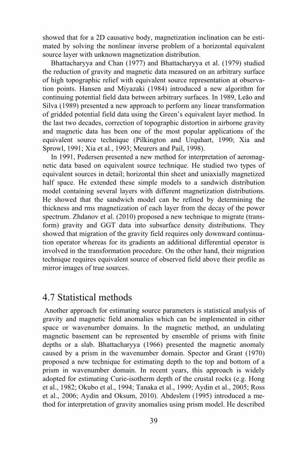
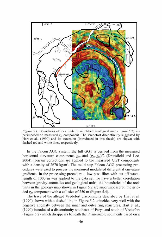
Figure 5.4. Boundaries of rock units in simplified geological map (Figure 5.2) su-perimposed on measured gzz component. The Vredefort discontinuity suggested by Hart et al., (1990) and its extension (introduced in this thesis) are shown with dashed red and white lines, respectively.

In the Falcon AGG system, the full GGT is derived from the measured horizontal curvature components gxy and (gxx-gyy)/2 (Dransfield and Lee, 2004). Terrain corrections are applied to the measured GGT components with a density of 2670 kg/m3. The multi-step Falcon AGG processing pro-cedures were used to process the measured modulated differential curvature gradients. In the processing procedure a low-pass filter with cut-off wave-length of 1000 m was applied to the data set. To have a better correlation between gravity anomalies and geological units, the boundaries of the rock units in the geology map shown in Figure 5.2 are superimposed on the grid-ded gzz component with a cell size of 250 m (Figure 5.4).

The trace of the alleged Vredefort discontinuity described by Hart et al. (1990) shown with a dashed line in Figure 5.2 coincides very well with the negative anomaly between the inner and outer ring structures. Hart et al., (1990) introduced a discontinuity southeast of Parys and south of Vredefort (Figure 5.2) which disappears beneath the Phanerozoic sediments based on a

47

broad negative magnetic anomaly that can give a good pattern for the core of the dome. This discontinuity separates the lower (ILG) and upper (OGG) crust. Based on the negative gravity anomaly separating the inner and outer ring structures (Figure 5.4), this discontinuity can be extended further to the south crossing the Greenstones in southeast of the Vredefort dome (Figure 5.4). In Figure 5.4, the Vredefort discontinuity suggested by Hart et al., (1990) and its extension (introduced in this thesis) are shown with dashed red and white lines, respectively.

5.2 The Särna area, west central Sweden Särna is located 450 km north west of Stockholm. Most of the geological units of the study area are dated between Paleoproterozoic to Neoprotero-zoic. Bylund and Patchett (1977) describes that the age of the nepheline syenite of Särna exposed on the hills Siksjöberget located about 15 km west of Särna is estimated the Permian (0.292–0.250 Ga). This circular body which is the youngest geological unit in the area with about 4 km diameter is intrusive into the Dala porphyries, rhyolite and trackydacite rocks, dated at 1.87–1.66 Ga (Welin and Lundqvist, 1970). Other lithologies include sandstone and intrusive dolerite of Precambrian age. Figure 5.5 shows the simplified geology of the Särna area provided by the Geological Survey of Sweden (SGU) in 2010. This figure shows that dolerite dikes are dominant geological features. The Neoproterozoic dolerite dikes (1–0.54 Ga) are in-trusive to most of the rock units except the young nepheline syenite. The dominant strike direction of the dolerite dikes is NW-SE. The most interest-ing geophysical feature of this area is the dolerite dike exposed as a ring structure in the center of the study area.

5.2.1 Aeromagnetic data from the Särna area The Särna area was covered with aeromagnetic measurements during years 2004 and 2005 in three campaigns conducted by SGU. The nominal height of the aircraft was 60 m above the ground with a sampling interval of about 17 m along the flight lines. The flight lines were flown in E-W direction with spacing of 200 m, 400 m and 800 m for areas 1, 2 and 3, respectively (see Figure 6a in paper II). Figure 6a of paper II shows the gridded total magnetic anomaly with cell size of 200 m after applying the low pass filter of 400 m and re-sampling the filtered data with 200 m sample interval in both x and y directions.

48

Fig

ure

5.5.

Geo

logy

map

of

the

Sär

na a

rea

(with

per

mis

sion

fro

m S

GU

).

49

6. Summary of papers

This thesis is based on four papers which are summarized in this chapter. The summary of papers involves a brief description of the main objectives, developed methods and their application to real data examples, conclusions and my individual contribution to each paper.

6.1 Paper I: Eigenvector analysis of GGT to locate geologic bodies 6.1.1 Summary This paper introduces a new method for interpretation of GGT data which is developed based on Pedersen and Rasmussen (1990). They studied gradient tensors of gravity and magnetic fields and introduced scalar invariants to indicate their dimensionality. They also showed that the eigenvector v1 cor-responding to the maximum eigenvalue of the GGT points towards the cen-ter of mass for a simple point source. In paper I, we show that the strike direction of a quasi 2D body can be estimated from the projection of the eigenvector corresponding to the smallest eigenvalue onto the horizontal plane.

For a compact body of arbitrary shape, the eigenvector v1 will be directed approximately towards the center of mass which can be approximated by an equivalent point source. Such an equivalent source location can then be es-timated from a collection of observation points located within a given win-dow whose gravity field is predominately generated from the same body. The eigenvector v1 which satisfies equation 01vrr denotes a straight line passing through the observation point P(x, y, z). The distance from the equivalent point source P0 to this line is given by

1

01

vrrv

d (6.1)

where 11v . Then, the distance from the source point to the line passing

through each observation point Pi (xi, yi, zi) parallel to the eigenvector v1 at Pi can be determined by minimizing the expression

50

N

i

idQ1

2 (6.2)

where N is the number of observation points in the window. Assuming that maxima or minima of the gzz component occurs approxi-

mately above the center of mass for positive or negative anomalies, respec-tively, a window centered on the located maximum or minimum is formed. With larger windows more eigenvectors are used to estimate the source lo-cation, and generally the accuracy of the estimated depth is improved sig-nificantly. However, in the case of real data, eventually eigenvectors may become more influenced by neighboring sources. The algorithm is improved by removing eigenvectors with distances to the estimated source location larger than a threshold value (20%) and the procedure is repeated.

In our algorithm, we increase the window size until the window size ex-ceeds a predefined limit which is defined by user based on the bandwidth of the data. Solution corresponding to the window with minimum standard error is then chosen as the final source location. In order to study the effect of additive random noise and interfering sources, the method is tested on synthetic data examples and it appears that our method is robust to random noise in the different measurement channels. The application of the method is demonstrated on a GGT data set from the Vredefort impact structure, South Africa.

6.1.2 Conclusions The application of the introduced method to a GGT data set from the Vrede-fort dome area provided very stable depth estimates along the ring struc-tures. The estimated depths along the inner rings are predominantly in the range 1000 to 1500 m and outer rings are predominantly exceeding 1500 m. In the central uplift part they are somewhat more scattered with most esti-mates exceeding 1500 m.

Comparing the results of the method with the results of Euler deconvolu-tion of GGT shows that Euler deconvolution by its very nature better out-lines the edges of the causative bodies whereas our method is more focused on the center of mass. Using our method we can easily distinguish between positive and negative anomalies of gzz and therefore produce two maps of depths and strikes. By this discrimination our maps become more easily interpretable. We conclude that the combination of Euler deconvolution and eigenvector analysis provides very useful complementary information which adds to the interpretative power of GGT data.

51

6.1.3 Contribution I carried out the theoretical derivations of eigenvector analysis of GGT and developed the least squares algorithm by the help of second author. I did the programming and numerical tests illustrated in this paper. The discussion and conclusions drawn in this paper are result of a cooperative of both au-thors. I wrote the manuscript but it was largely improved by second author.

6.2 Paper II: Interpretation of aeromagnetic data using eigenvector analysis of PGGT 6.2.1 Summary The pseudo gravity gradient tensor (PGGT) can be expressed in matrix form;

T

k

ik

k

ik

k

ik

k

k

k

kk

k

ik

k

kk

k

k

MC

yx

yyyx

xyxx

fmm

FF 1-

1

12

2

2

22

2

(6.3)

where F and -1F denote Fourier transformation and inverse Fourier trans-formation, kx and ky are wavenumbers in x and y directions and

22

yx kkk , m and f are phase factors of magnetization and induced

field with vectors of zyx mmm ˆ,ˆ,ˆ and zyx fff ˆ,ˆ,ˆ , respectively (Blakely,

1995). In paper II, we show that the same properties of the GGT are valid for the

PGGT derived from magnetic field data. Assuming that the magnetization direction is known, we extended the method introduced in paper I to PGGT for interpretation of magnetic sources. Eigenvectors of the PGGT are used to estimate depth to the center of mass of geological bodies as well as the strike directions of 2D geological structures.

The dimensionality of the pseudo-gravity field is defined from the dimen-sionality indicator I, derived from the tensor components. In the case of a quasi 2D structure, the horizontal gradient of the field along the strike of the causative body is very small. Employing the eigenvectors located along the strike direction may increase the uncertainty of the least squares procedure. To improve the performance of the introduced algorithm for 2D structures, a rectangular window with a length a few times greater than its width and perpendicular to the strike of the 2D structure is used for estimating the

52

source location. The ratio between the length to the width of the rectangular window is defined based on the dimensionality indicator I.

To study the effect of remanent magnetization on depth estimates, the method is applied to synthetic examples. Our numerical tests show that depth estimates are more affected by the difference between the inclination of the induced field and magnetization vector I, than the difference be-tween their declinations D. We have also studied the effect of remanent magnetization on strike estimation of 2D bodies by analysis of simple ge-neric models. These generic models show that the strike estimates are af-fected by remanent magnetization direction with deviations from pure 2D conditions whereas in the case of a 2D structure with infinite depth and strike length (a purely 2D field) remanent magnetization has no effect on estimated strikes.

6.2.2 Conclusions The method is applied to the magnetic field data from the Särna area, west central Sweden, to estimate depths to the center of mass of geological bodies as well as the strike direction of quasi 2D structure. Depth estimates along the linear features are very stable showing that most of the dolerite dikes are very shallow. This agrees with the geological information which show that these dikes outcrop on the surface.

As was discussed in paper I, comparing our method with Euler deconvo-lution shows that our method is rather insensitive to random noise while use of derivatives of the field in Euler deconvolution may amplify the random noise. Euler deconvolution gives better solutions for anomalies caused by sources suffering from interference effects whereas the eigenvector analysis method provides more reliable results for anomalies with small gradients of the field than Euler deconvolution. It is also shown that depth estimates derived from the proposed method are influenced by remanent magnetiza-tion when the solutions of Euler deconvolution are independent of magneti-zation direction

6.2.3 Contribution I did the programming and numerical tests used in this paper. The geological description provided in this paper is result of cooperation between first and third authors. I wrote the manuscript but it was modified by second author.

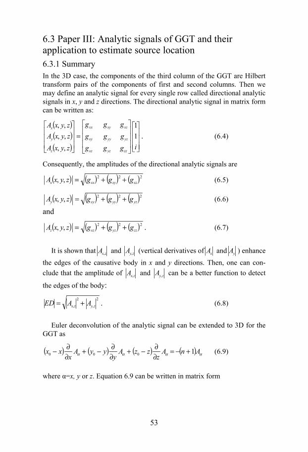
53

6.3 Paper III: Analytic signals of GGT and their application to estimate source location 6.3.1 Summary In the 3D case, the components of the third column of the GGT are Hilbert transform pairs of the components of first and second columns. Then we may define an analytic signal for every single row called directional analytic signals in x, y and z directions. The directional analytic signal in matrix form can be written as:

iggg

ggg

ggg

zyxA

zyxA

zyxA

zzyzxz

yzyyxy

xzxyxx

z

y

x

1

1

,,

,,

,,

. (6.4)

Consequently, the amplitudes of the directional analytic signals are

222,, xzxyxxx gggzyxA (6.5)

222,, yzyyxyy gggzyxA (6.6)

and

222,, zzyzxzz gggzyxA . (6.7)

It is shown that zxA , and zyA , (vertical derivatives of xA and yA ) enhance

the edges of the causative body in x and y directions. Then, one can con-

clude that the amplitude of zxA , and zyA , can be a better function to detect

the edges of the body:

2

,

2

, zyzx AAED . (6.8)

Euler deconvolution of the analytic signal can be extended to 3D for the GGT as

AnAz

zzAy

yyAx

xx 1000 (6.9)

where =x, y or z. Equation 6.9 can be written in matrix form

54

zzzz

yyyy

xxxx

zzzz

yyyy

xxxx

Az

Az

y

Ay

x

Ax

Az

Az

y

Ay

x

Ax

Az

Az

y

Ay

x

Ax

N

z

y

x

Az

A

y

A

x

A

Az

A

y

A

x

A

Az

A

y

A

x

A

0

0

0

.

(6.10)

By applying Euler’s equation (equation 6.10) to the GGT data, the location and structural index of the causative body is estimated within a sliding win-dow with adjustable size. Assuming that maxima of the edge detector func-tion, ED occurs approximately above the edges of causative bodies, a win-dow centered at the located maximum is formed. The computational time and number of solutions decrease significantly by locating the center of the square window at the predefined maxima of the function ED .

The relative estimated error, the standard error normalized by the corre-sponding estimated depth, is used to provide a better explanation of the error distribution for solutions with respect to the estimated depth. The following criteria are used in the presented algorithm to discriminate between solu-tions;

1- The estimated source locations with standard deviation-to-estimated depth ratio greater than a threshold which is defined by user are re-jected.

2- Only those solutions with horizontal coordinates located within the window are accepted.

3- Solutions with estimated depths greater than a predefined threshold (by user) are rejected.

4- Solutions with unreliable estimated structural indices are rejected.

The application of the method is demonstrated on gravity gradient tensor data in the Vredefort impact structure, South Africa.

6.3.2 Conclusions The introduced directional analytic signals can be used to detect the edges of causative bodies. It is shown that the edge detector function ED enhances the edges of causative bodies better than the horizontal gradient amplitude, HGA when the causative body is interfered by neighboring sources laterally and vertically.

The amplitudes of directional analytic signals are homogenous and sat-isfy the Euler’s homogeneity equation. The advantage of this method is that the constant base level is removed from the Euler’s equation. Then the struc-tural index and source location can be estimated from Euler deconvolution of the directional analytic signals directly. This improves the conventional

55

Euler deconvolution using three gradients of the vertical component of the gravity vector. It is also shown that the Euler deconvolution of the direc-tional analytic signals estimates the source location better than the conven-tional Euler deconvolution of GGT when the causative is interfered by neighboring sources. The disadvantage of the presented method is that they are more sensitive to noise than the conventional ones. Using upward con-tinuation of the gravity gradient tensor data, the noise effect can be reduced.

6.3.3 Contribution In this work, I developed the idea of combining analytic signals of GGT and Euler’s homogeneity equation to estimate source location. I did program-ming, numerical tests and manuscript writing alone. However, the com-ments made by Professor Laust B. Pedersen and other reviewers improved this work considerably.

6.4 Paper IV: Deconvolution of GGT data using infinite dike and geological contact models 6.4.1 Summary For infinite dike and geological contact models striking in the y direction, the measured gxz and gzz components can jointly be inverted for estimating the five model parameters horizontal position, depth to the top, thickness, dip angle and density contrast for infinite dike and geological contact mod-els.

In the introduced technique, we solve the nonlinear equations of infinite dike and geological contact models for estimating corresponding model parameters in a line segment containing several data points measured ap-proximately above the causative body. Assuming that the segment is suffi-ciently large, the parameter estimation problem is overdetermined. The Le-venberg-Marquardt (LM) algorithm is used to minimize the nonlinear objec-tive functions describing data fit over parameter space together with a quad-ratic programming approach allowing for upper and lower bounds on parameters.

Data and model parameters are related through a nonlinear system of eq-uations g(m)=d and the objective function to be minimized is

mn

rs

n

i

i

1

2

(6.11)

56

where ri=g (mest )i- di ; i=1, 2,…, n, n and m are the number of data points and model parameters, respectively, mest is the estimated model parameters and the data vector d include both gxz and gzz.

To reduce the effect of interfering sources, a window is formed around the maximum of gzz. Data points enclosed by this window are used in the inversion scheme for estimating the parameters and the position of the dike. In the case that the window length is very small, the dike parameters cannot be estimated accurately. In the presence of random noise, a large window size is preferred to overcome the effect of local high frequencies. However, use of a very large window is also risky as we may include data points which are more affected by neighboring bodies. We define an optimum window length based on the data fit error.

Investigating different synthetic data sets show that we normally are able to exclude inappropriate models based on a data fit criterion or because of scattered or unphysical solutions. To avoid unphysical estimates, we define constraints with lower and upper bounds on the model parameters so that solutions are always in the trust region. For real cases, any a priori informa-tion of the geology can be used either as constraints or criteria to reject spu-rious solutions.

As was shown in paper I, for a given measurement point, the strike direc-tion of the GGT caused by a quasi 2D structure is estimated from the eigen-vector corresponding to the smallest eigenvalue. Then, the measured com-ponents can be transformed into the strike coordinate system. In the case of gridded data and assuming that the maximum of gzz is approximately located above the causative body, all measurement points enclosed by a square win-dow centered at the maximum of gzz are used to estimate the source parame-ters.

We applied our method to a GGT data set from the Vredefort impact structure in South Africa. The physical and geometrical parameters of the major geological features of dike like bodies and/or geological contacts in the study area are estimated using the deconvolution technique introduced in paper IV.

6.4.2 Conclusions In practice, airborne gravity gradiometry surveys are collected along parallel lines crossing the dominant strike direction of 2D geological structures. For the deconvolution, we use data points located within a square window cen-tered at maxima of gzz. To improve the reliability of the estimated source parameters, some geological constraints are used in the inversion scheme. The measured gxz and gzz components are jointly inverted for estimating the source parameters for infinite dike and geological contact models.

The ratio between the estimated data fit errors for infinite dike and geo-logical contact models are used to discriminate the spurious model types.

57

This discrimination between dike and geological contact models based upon the data fit error criterion works very well for both theoretical and real cas-es. In the real case shown in this paper, the distribution of the data fit error for the two models and their ratio indicate mean data fit errors of 2.87 ± 1.01 E and 10.70 ± 5.35 E for dike and contact models, respectively.

The different parts of the Vredefort impact area such as the dense central part, dense ring structures and less dense metasediments are delineated very well by deconvolving the GGT data. Using geological constraints and dis-crimination criteria, all major 2D geological structures in the dome area can be modeled as thick dikes. Depth estimates along the major geological fea-tures are stable predominantly around 1000 m. Inferred strikes of the thick dikes are concentric to the center of the dome and they are subvertical and outward dipping for the two inner ring structures and inward dipping for the outer ring.

6.4.3 Contribution I carried out the theoretical derivations of the nonlinear least squares algo-rithm for inversion of two dimensional GGT components under supervision of second author. I did the programming and numerical tests illustrated in this paper. Both authors contributed equally to the interpretation of the real data example. I wrote the manuscript but it was improved by second author considerably.

58

59

7. Discussion and conclusions

This thesis focuses on the development of new processing and interpretation techniques for GGT data as well as PGGT derived from measured magnetic field data. The proposed methods in this thesis are applied to a recent GGT data set from the Vredefort impact structure, South Africa and an aeromag-netic data set from the Särna area, west central Sweden. The implementa-tions of the introduced methods are improved using sliding windows, dis-crimination of solutions, incorporating geological constraints and combining with results of complementary methods. In this chapter I describe the most important aspects of the methods and results achieved.

7.1 Discussion 7.1.1 Application of sliding windows in the source parameter estimation techniques Many processing and interpretation techniques (e.g. Euler deconvolution and Werner deconvolution) of gravity and magnetic data employ overlap-ping sliding windows to reduce the effect of random noise and interfering sources. Uncertainty of solutions acquired for every single window is in-creased when a window does not include any significant variations of the gravity or magnetic field or when it includes variations caused by different sources.

In the case that causative sources are close together, the smallest window possible is preferred. However, broad anomalies caused by deep sources are poorly estimated using a small window. In the introduced methods, we have shown that the optimum window size can be chosen based on the uncer-tainty of the solutions acquired for different window sizes. In paper II it is also shown that, in the case of 2D field, the results can be further improved by employing a rectangular window with its length perpendicular to the estimated strike direction of the causative 2D body.

To reduce the number of solutions and computational time, windows are centered at maxima of gzz (papers I, II and IV) or maxima of the edge detec-tor function introduced in paper III depending upon the method used for estimating the source location.

60

7.1.2 Discrimination of solutions and geological constraints In paper I, II and III, It is described that the uncertainty of the estimated source location can be calculated from the least squares solution of the overdetermined set of equations. The total uncertainty of the estimated source location contains the estimated errors of x, y and z coordinates of solution. The total uncertainty normalized by the corresponding estimated depth is used as a criterion to discriminate more reliable solutions from spu-rious ones. Furthermore, solutions with horizontal coordinates located out-side the window, estimated depths greater than a given threshold or solu-tions with negative estimated depths are rejected. In paper III, the estimated structural index is used as a discrimination criterion in addition to the crite-ria above.

In paper IV, we have used a quadratic programming allowing for upper and lower bounds on source parameters. To avoid unphysical estimates (e.g. negative depth, thickness, width and unreliable density contrast), some con-straints are defined so that solutions are always in the trust region. In addi-tion, the solutions with a horizontal distance to the center of the window greater than a given threshold are rejected. For real cases, any other a priori information of the geology can be used either as constraints or rejection criteria to refine solutions.

We have also shown that the discrimination between infinite dike and geological contact models based upon the data fit error acquired for each model type works surprisingly well. We also studied incorporation of low order polynomials representing interference effects in the presented decon-volution scheme. We found that the low order polynomials could accommo-date significant parts of the signal and thus make the discrimination between the model types less distinct.

7.1.3 Improvement of results using complementary methods Interpretation of GGT or magnetic data using the introduced methods can be significantly improved by incorporating complementary methods. In paper I, it is shown that tensor Euler deconvolution of GGT can be used to delineate the edges of causative bodies whereas eigenvector analysis of GGT data provides useful estimates of depth to the center of mass as well as strike direction of quasi 2D bodies.

In paper II, eigenvector analysis of PGGT derived from magnetic field data is compared with Euler deconvolution of magnetic field. Combining the results of these methods has considerably improved interpretation of the aeromagnetic data from the Särna area, west central Sweden. The Euler deconvolution employs first order derivatives of the magnetic field whereas the eigenvector analysis uses pseudo-gravity gradients. It is also described that Euler deconvolution provides more reliable solutions for anomalies with

61

high gradients of the field while the eigenvector analysis of PGGT data gives better estimates for long wavelength anomalies.

Euler deconvolution of directional analytic signals of GGT data (paper III) is compared with tensor Euler deconvolution. The advantages and dis-advantages of each method are studied with synthetic and real data exam-ples. Results of the deconvolution technique introduced in paper IV can be combined with analytic methods developed for estimating dike and contact model parameters (e.g. Hsu et al., 1998; Bastani and Pedersen, 2001). These methods were initially developed for the magnetic case but can easily be adopted for interpretation of GGT data.

7.2 General conclusions The main objective of this thesis was to develop new processing and inter-pretation tools for GGT data. The eigenvectors of GGT provide useful in-formation about depth to the center of mass for 3D causative bodies as well as the strike direction of quasi 2D structures. The same properties are valid for PGGT derived from magnetic field data assuming that magnetization direction is known. It is also shown that in the presence of interference ef-fects estimation of source location can be improved using Euler deconvolu-tion of directional analytic signals in x, y and z directions.

In 2D cases, the estimated strike direction using eigenvector analysis of GGT or PGGT can be used to correct the measured gravity or magnetic field for the effect of deviation of the angle between measured profile and strike of 2D sources from the normal. The source parameters horizontal position, depth to the top, dip angle, width, thickness and density contrast of infinite dike and geological contact models can be estimated using deconvolution of GGT components. To improve the reliability of the estimated source pa-rameters, geological constraints can be used in the inversion scheme. The developed methods for interpretation of GGT data may also well be suited for magnetic gradient tensor.

Applications of the introduced methods (papers I, III and IV) to the GGT data set from the Vredefort dome shows that the different parts of the struc-ture such as the dense central part, dense ring structures and less dense me-tasediments are delineated very well. Depth estimates along the major posi-tive anomalies are stable around 1000 m. The estimated strikes of these 2D features are concentric to the center of the dome and they are subvertical and outward dipping for the two inner ring structures and inward dipping for the outer ring.

The method described in paper II is applied to magnetic field data from the Särna area to estimate depths to the center of mass of geological bodies as well as the strike direction of quasi 2D structure. Depth estimates along the linear features are very stable. The results of our method show that most

62

of the dolerite dikes are very shallow. This agrees with the geological in-formation which show that these dikes outcrop on the surface.

7.3 Future developments The eigenvector analysis introduced in papers I and II can be employed for interpretation of measured GGT or magnetic gradient tensor (MGT) data measured along profiles. GGT data can be directly used for estimating source locations dimensionality analysis. MGT data need to be transformed to PGGT data before source locations can be estimated. Such transforma-tions can be carried out along profiles provided sufficiently long sections of 2D data.

To reduce the effect of the regional field on strike estimates, a high pass filter can be applied to data prior to calculation of eigenvectors. An alterna-tive approach to the method proposed in paper III is Euler deconvolution of the Hilbert transform of GGT data. The constant base levels of gravity gra-dients are then removed from Euler’s equation and the structural index and source location can be estimated directly from Euler deconvolution of Hil-bert transformed GGT data.

The deconvolution technique presented in paper IV can be further devel-oped using any simplified model such as sphere, vertical semi-infinite cylin-der (pipe) or rectangular prism.

63

8. Summary in Swedish

I ett kartesiskt koordinatsystem innehåller gravitationsfätets gradienttensor (GGT) andraderivatorna av potentialen för jordens gravitationsfält i de tre ortogonala riktningarna. GGT-data kan mätas med antingen mark- , luft-, marin- eller rymdplattformar. Under de senaste två årtiondena har tillämp-ningar av GGT-data i prospektering efter kolväten och mineral och i struk-turgeologiska undersökningar ökat avsevärt.

Detta arbete fokuserar på att utveckla nya tolkningstekniker för GGT-data samt för pseudo-gravitationsfältets gradienttensordata (PGGT-data) beräknade från uppmätta magnetfält. Tillämpningar av de utvecklade meto-derna visas på GGT-data från impaktstrukturen Vredefort, Sydafrika, och på magnetfältdata från Särnaområdet i nordvästra Dalarna, Sverige.

8.1 Egenvektoranalys av GGT- och PGGT- data (artiklarna I och II) Egenvektorer av den symmetriska GGT kan användas för att uppskatta såväl läget av en störkropp som dess strykningsriktning. För en given mätpunkt pekar den egenvektor, som motsvarar största egenvärdet, ungefär mot stör-kroppens tyngdpunkt. För en samling mätpunkter, som ligger inom ett kva-dratiskt fönster, har en robust algoritm, baserad på minstakvadratmetoden, utvecklats för att uppskatta störkroppens centrum som punkten med minsta kvadratsumma av avstånden till de linjer som går igenom mätpunkterna och är riktade som egenvektorerna. För en kvasi-2D störkropp kan stryknings-riktningen beräknas från den egenvektor som motsvarar det minsta egenvär-det. Samma egenskaper som gäller för GGT gäller för pseudo-gravitationsfältets gradienttensor (PGGT) från magnetfältdata förutsatt att magnetiseringsriktningen är känd och är konstant.

8.2 Analytiska signaler av GGT för uppskattning av djup till störkroppar (artikel III) Beräkning av analytisk signal tillämpas på GGT-data i tre dimensioner. Tre analytiska signaler införs i x-, y-och z-led och kallade riktade analytiska signaler. De riktade analytiska signalerna är homogena och uppfyller Eulers

64

homogenitetsekvation. Eulerdekonvolution av riktade analytiska signaler kan användas för att lokalisera orsakande störkroppar. Störningseffekter från angränsande källor minskas genom derivering av de riktade analytiska sig-nalerna i x-, y-och z-riktningarna. Dessutom uppskattas det strukturella in-dexet för gravitationsfältet automatiskt genom att lösa de tre Eulerekvatio-ner, som härrör från GGT för en uppsättning datapunkter inom ett kvadra-tiskt fönster med justerbar storlek.

8.3 Dekonvolution av GGT-data med hjälp av modeller för oändliga geologiska gångar och kontakter (artikel IV) För 2D störkroppar med strykning i y-riktningen kan gxz- och gzz-komponenterna av GGT inverteras tillsammans för att uppskatta parametrar i modeller för oändlig geologisk gång och kontakt. När strykningsriktningen av den orsakande störkroppen är beräknad, kan de uppmätta komponenterna av GGT transformeras till det strykningsorienterade koordinatsystemet. Mätpunkter inom ett kvadratiskt fönster används för att uppskatta störkrop-pens parametrar. Efter dekonvolvering av GGT-data inom en uppsättning kvadratiska fönster med både gång- och kontaktmodeller, väljs slutligen den bästa modellen utifrån bästa dataanpassning.

65

9. Acknowledgements

This work would not have been possible without the help, support and en-couragement of many people and I would like to take this opportunity to express my gratitude to them.

I am particularly grateful to my supervisor Professor Laust B. Pedersen who accepted me as a PhD student, gave me a great insight into applied geophysics and provided me with freedom in the research topics to follow my interests. I greatly appreciate his valuable comments on my papers. He spent many constructive hours helping me to formulate my ideas. I appreci-ate the time and effort he put into reading my manuscripts to make them comprehensible.

I would also like to thank my second supervisor Dr. Mehrdad Bastani for his constructive comments and valuable discussions which greatly improved my work. I should also express my appreciation to his wife Fariba. I do not know how to appreciate your friendship during these years. Dear Mehrdad and Fariba, thank you from bottom of my heart.

During my stay in Uppsala, I have found many new friends. Their friend-ship made my life a pleasure. I thank Naser Matori and his wife Afsaneh, Taher Mazloomian and his family, Faramarz Nilfouroushan and his wife Tabasom, Alireza Malehmir and Azita Dehghannejad, Jahangir Taghian and his wife Pooran, Farnoosh Rezaee, Hesam Kazemeini and his wife Masoo-meh, Aziz Nasuti and his wife Kurdestan, Saied Cheraghi and his wife Far-zaneh, Marie Keiding, Sawasdee Yordkahun, Emil Lundberg, Peter Schmidt, Jochen Kamm, Ismail Nazli, Abigail Barker, Artem Kashubin, Thomas Kalscheuer, Niklas Juhojuntti, Anna Ladenberger, Kristín J nsdóttir, Eva Lindblom, Tuna Eken, Maria Garcia, Can Yang, Fengjiao Zhang, Juliane Hübert, Milad Elmaradi, Amir Abdi, Arnaud Pharasyn, Pálmi Erlendsson and Nina Ivanova.

I would like to thank the academic and support staff from Department of Earth Sciences specially; Prof. Chris Juhlin, Dr. Chris Hieronymus, Prof. David Gee, Prof. Dan Dyrelius, Prof. Hemin Koyi, Mr. Lars Dynesius, Dr. Ari Tryggvason, Mr. Taher Mazloomian, Mrs. Siv Petterson, Mrs. Ingegerd Ohlsson, Mrs. Susanne Paul, Mr. Tomas Nord and Mr. Leif Nyberg.

66

I appreciate Dr. Mark Dransfield from Fugro Airborne Surveys for his constructive comments on two of my papers and providing the GGT data set from the Vredefort dome as well as useful resources for writing my thesis and also Dr. Lutz Kübler from SGU for geology description of the Särna area. I would also like thank to Dr. Lena Persson and Dr. Ildiko Antal-Lundin from SGU.

I would like to acknowledge Professor Laust. B. Pedersen, Dr. Mehrdad Bastani and Dr. Faramarz Nilfouroushan for their constructive comments on this thesis.

I have left the most important people until last; my parents, Mohammad and Farideh, my brother Mohsen and my beloved wife Hediyeh. I greatly appreciate my parents for all they have given me in life and for encouraging me to pursue my education. I am very sorry that I have not been beside you during past three years when Mohsen was ill. Mom, you have been fighting cancer for a long time, you are my hero. Dad, Mom, you are wonderful!

I would also like thank Flora, Hediyeh’s mother, for encouraging me dur-ing last two years with my PhD research. Dear Flora, you always have been as kind as a mother to me. Thank you!

Dear Hediyeh, today it is exactly two years and two months that we have been living together. I deeply appreciate your support during this period. I am sure that I would never have made it without the confidence you gave me. You always encourage me to go further with my studies and wish me success from bottom of your heart.

Hediyeh, you have given me your love and this is the most valuable thing that I have in my life. Thank you!

December 5, 2010 Uppsala

67

A. Additional notes on impact structures

A.1 Impact craters The term impact crater is used for any approximately circular depression on the surface of a planet or any other solid body in the Solar System caused by the hyper-velocity impact of a bolide with the surface. In contrast to vol-canic craters which are formed by explosion or internal collapse, impact craters typically have rims higher and floors lower than the surrounding terrain. On some planets like the Earth which has experienced active geo-logical processes, impact craters are less visible as they are eroded, buried or transformed by tectonics over time. In such cases the original crater is de-stroyed, and the term impact structure is more commonly used. More than 170 impact structures with diameters ranging from a few tens of meters up to 300 km are identified on Earth. Their ages range from very recent impact craters in 1947, the Sikhote-Alin in Russia, to more than two billion years (in the paleoproterozoic era), the Vredefort impact structure in South Africa.

A.2 Impact cratering In the case of hyper-velocity impacts, both impactor and target rocks are melted and vaporized partially. Impacts at speeds higher than velocity of sound produce shock wave in solid materials. Then impactor and the im-pacted surface materials are compressed considerably to form high density materials. Because of arbitrary size of impactors, the kinetic energy released into the Earth and subsequently geological processes may be extremely large. This is very different to normal geological process like volcanism as a huge amount of energy is released in a few seconds. Melosh (1989) divided the impact process into three distinct stages; contact and compression, exca-vation and modification.

A.2.1 Contact and compression When a hyper-velocity projectile contacts the surface, target materials are pushed out of the projectile’s path. Density of the materials between the projectile and surface is increased considerably because of the strong com-pression and subsequently shock waves are created around the contact area. At the same time, the resistance to penetration decelerates the projectile

68

(Melosh, 1989). When the projectile penetrates into the ground, shock pres-sure increases until it exceeds the yield strength of both the projectile and surface materials. In this stage they may melt or vaporize as the shock wave raises the temperature of the materials (Figure A.1). In the case of small impacts, this temperature is sufficient to melt the impactor. The contact and compression stage ends when the high pressure of the projectile decays.

Figure A.1. a) Contact and b) compression stage.

A.2.2 Excavation After the contact and compression stage, the excavation begins by moving the target materials away from the contact point. By growing the cavity, a bowl-shaped crater is produced in which its center is pushed downwards, a large volume of the surface materials are ejected and its elevated crater rim is formed. In the case of vertical impacts, normally the produced transient cavity is hemispherical. Hyper-velocity impacts usually create crater’s di-ameter much larger than sub-sonic impacts (Melosh, 1989).

During this stage, shock wave propagates into the target rocks and it di-minishes by expanding into more materials. A small portion of the melt rocks are ejected while a significant part remains inside the transient cavity (Figure A.2). The melt rock zone follows the vaporized zone and further down when shock energy is decreased rocks are fractured and brecciated (Figure A.1b). The ejecta cover the terrain around the crater within a few crater radii.

A.2.3 Modification In the modification stage, the transient crater remains as a simple bowl-shaped crater or develops into a complex crater exhibiting a central uplift or with several interior and exterior rings. This depends upon the size of the craters as well as physical properties of target materials. In this stage, the steep interior walls slide down and fill the transient cavity with collapsed breccia, ejecta and melt rocks.

69

For small transient craters, modifications are not significant. The original shape of the transient crater is preserved and the excavated crater remains as a bowl-shaped crater. In the case of large transient craters, the modifications are significant because of elastic rebound and collapse of the elevated rim under gravity. Then central uplifts and ring systems are formed a group of craters called complex craters (Figure A.2).

Figure A.2. Excavation and modification stages. (Image courtesy B. M. French and D. A. Kring, LPI).

70

A.3 Morphology of impact craters The impact structures produced by hyper-velocity impacts are categorized into three types; simple crater, complex crater and multi-ring basins (Me-losh, 1989). The difference between simple and complex craters is illus-trated in Figure A.3. Complex craters have a central peak while simple cra-ters are more bowl-shaped. According to this classification, most of the con-firmed impact structures on the Earth are considered to be either simple or complex type. Hawke (2004) describe that the distinction between simple and complex craters is very straightforward but there is some confusion about definition of multi-ring structures. He clearly states that the only con-firmed examples for true multi-ring basins are found on other planetary bod-ies in the Solar System. This is in contradiction with Grieve and Therriault (2000) which states that there are some confirmed multi-ring basins on the Earth e.g., the Vredefort, Sudbury and Chicxulub. They also mention that the only example with morphological ring features is the Chicxulub basin in Mexico.

A.3.1 Simple craters Simple crater have the classic form of bowl-shaped depression (Hawke, 2004). Figures A.3a and b show an image of a typical simple crater in Ari-zona, USA and a schematic diagram of a simple crater, respectively. The raised rim of the crater usually overturns due to the excavation of the tran-sient cavity. A layer of brecciated rocks resulting from slumping of the tran-sient crater walls covers the floor of the crater (Westbroek and Stewart, 1996).

A.3.2 Complex craters Generally, there is a transition diameter between simple and complex cra-ters. An abrupt change in morphology of lunar craters takes place at diame-ters 10-20 km (Melosh, 1989) while on Earth this diameter is 2-4 km. This depends upon surface gravity and target rock type (Pilkington and Grieve, 1992). In the case of large craters, because of steepness of the walls, they collapse under gravity to form a more complex shape and their floors are filled with brecciated and melt rocks. Main characteristics of complex cra-ters are shallow crater floors, central uplifts and terraces within the inner wall of the crater (Hawke, 2004). Figures A.3c and A.3d show an image of complex crater Tycho on the Moon and a schematic cross section of a com-plex crater, respectively.

Westbroek and Stewart (1996) describe that both simple and complex craters have a depth to diameter ratios of 1/4 to 1/3. They also state that because of the slumping, the transient crater diameter extends by almost 20% to form the final crater diameter. Grieve and Pilkington (1996) shows

71

that the terrestrial central peak is related to transient crater through the em-pirical relation

SU=0.086 D1.03 (A-1)

where SU is the amount of structural uplift now exposed at the surface and D is the crater diameter.

Figure A.3. a) A simple crater in Arizona, USA, b) a simplified cross section of a simple crater, c) a complex crater, Tycho on the Moon and d) a simplified cross section of a complex crater. (Image courtesy NASA).

A.3.3 Multi-ring craters Spudis (1993) defined multi-ring basins as large impact structures that ini-tially had multi-ring morphology. Based on this definition, Grieve and Ther-riault (2000) categorized the large impact structures Vredefort (South Af-rica), Sudbury (Canada) and Chicxulub (Mexico) as multi-ring impact struc-tures.

The Earth planet is the most geologically active planet in the Solar Sys-tem. This is why the earliest morphology of most of the impact craters on Earth is not preserved. They are mainly eroded, covered with younger sedi-ments or strongly tectonized. This makes the morphological study of the impact structures on the Earth very difficult. As an example of multi-ring basins, I show the 4000 km diameter Valhalla basin on Callisto, Jupiter’s moon (Figure A.4). Tens of rings are identified around the crater which is probably represented by the approximately 800 km diameter light gray area in the middle of the image (Hawke, 2004).

72

Figure A.4. Valhalla basin on Jupiter’s moon, Callisto (Image courtesy NASA).

A.4 Gravity signature of impact craters In the cases that morphology of impact craters are covered by post-impact sediments, geophysics can provide valuable information about physical and geometrical properties of impact structures. Many terrestrial impact craters are initially identified based on their geophysical signature. In 1992, Pilk-ington and Grieve provided and excellent overview on geophysical signature of terrestrial impact structures worldwide. To date, many new examples for geophysical studies including gravity, magnetic, electromagnetic and seis-mic methods are reported in the literature.

Gravity is an important geophysical tool for recognition of impact struc-tures because of density changes of target rocks in the compression stage. For simple craters, gravity anomalies are generally circular with negative values which are caused by low-density brecciated and fractured rocks. The density contrast of the brecciated and fractured rocks depends on the diame-ter of crater as well as pre-impact density distribution of target rocks. For large complex craters e.g., the Vredefort dome in South Africa, the central part of impact structures show a relatively high gravity anomaly which is caused by central uplift.

Pilkington and Grieve (1992) described that the existence of a central up-lift in complex craters is not a sufficient condition for producing a high gravity anomaly. They showed that for complex craters with diameter smaller than 30 km, the gravity anomaly caused by central uplift can be highly dependent to the pre-impact density distribution of target rocks. They also studied the relation between observed density values and their corre-sponding depths for a borehole at Ries impact structure, Germany. Pilking-ton and Grieve (1992) showed due to the decrease in the level of shock-induced stress and thus fracturing with depth, density increases with depth.

73

References

Ameglio, L., 2005, New Fugro airborne gravity system – survey test over the Vredefort structure (South Africa). 67th EAGE Conference and Exhi-bition, Madrid, Spain, Extended Abstracts.

Aydin, I., H. I. Karat, and A. Kocak, 2005, Curie-point depth map of Tur-key. Geophysical Journal International, 162, 633-640.

Aydin, I., and E. Oksum, 2010, Exponential approach to estimate the Curie-temperature depth. Journal of Geophysics and Engineering, 7, 113-125.

Barbosa, V. C. F., J. B. C. Silva, and W. E. Medeiros, 1999, Stability analy-sis and improvement of structural index estimation in Euler deconvolu-tion. Geophysics, 64, 48-60.

Bastani M. and L. B. Pedersen, 2001, Automatic interpretation of magnetic dike parameters using the analytical signal technique. Geophysics, 66, 551-561.

Beiki M., 2010, Analytic signals of gravity gradient tensor and their applica-tion to estimate source location. Geophysics, 76, I59-I74.

Beiki M. and L. B. Pedersen, 2010, Eigenvector analysis of the gravity gra-dient tensor to locate geological bodies. Geophysics, 75, I37-I49.

Bell, R. E., R. Anderson, and L. Pratson, 1997, Gravity gradiometry resur-faces. The Leading Edge, 16, 55-59.

Bell, R. E., and R. O. Hansen, 1998, The rise and fall of early oil field tech-nology: The torsion balance gradiometer. The Leading Edge, 17, 81-83.

Bhattacharyya, B. K., 1966, A method for computing the total magnetization vector and the dimensions of a rectangular block-shaped body from magnetic anomalies. Geophysics, 31, 74-96.

Bhattacharyya, B. K., and K. C. Chan, 1977, Reduction of magnetic and gravity data on an arbitrary acquired in a region of high topographic re-lief. Geophysics, 42, 1411-1430.

Bhattacharyya, B. K., R. E. Sweeney, and R. H. Godson, 1979, Integration of aeromagnetic data acquired at different times with varying elevations and line spacings. Geophysics, 44, 742-752.

Blakely, R. J., 1995, Potential theory in gravity and magnetic applications. Cambridge University Press.

Bracewell, R. M, 1965, The Fourier transform and its applications. McGraw-Hill, Inc.

74

Brink, M. C., F. B. Waanders, and A. A. Bisschoff, 1999, Evolution of the ringed basin around Vredefort, South Africa. Meteoritics and Planetary Science, 34, A19-A20.

Boon, J. D., and C. C. Albritton, 1937, Meteorite scars in ancient rocks. Field lab, 5-53.

Bylund, G., and P. J. Patchett, 1977, Palaeomagnetic and Rb-Sr isotopic evidence for the ages of the Särna alkaline complex, western central Sweden. Lithos, 10, 73-79.

Dampney, C. N. G., 1969, The equivalent source technique. Geophysics, 34, 39-53.

Difrancesco, D., 2007, Advances and challenges in the development and deployment of gravity gradiometer systems. EGM 2007 International Workshop.

Dransfield, M. H., 1994, Airborne gravity gradiometry. The University of Western Australia, PhD thesis.

Dransfield, M. H., and J. B. Lee, 2004, The Falcon airborne gravity gradi-ometer survey systems. In R. Lane, ed., Airborne Gravity 2004, the ASEG-PESA Airborne gravity workshop, Australia, Extended Abstracts, 15-19.

Dransfield, M. H., and Y. Zeng, 2009, Airborne gravity gradiometry: Ter-rain corrections and elevation error. Geophysics, 74, I37-I42.

Dransfield, M. H., 2010, Conforming Falcon gravity and the global gravity anomaly. Geophysical Prospecting, 58, 469-483.

Droujinine, A., A. Vasilevsky, and R. Evans, 2007, Feasibility of using full tensor gradient (FTG) data for detection of local lateral density contrasts during reservoir monitoring. Geophysical Journal International, 169, 795-820.

Edwards, A. J., J. T. Maki, and D. G. Peterson, 1997, Gravity gradiometry as a tool for underground facility detection. JEEG, 2, 139-143.

Emilia, D. A., and R. L. Massey, 1975, magnetization-inclination estimation from prism-like anomaly profiles. Geophysics, 40, 443-450.

French, B. M., 2005, Stalking the Wily shatter cone: A critical guide for impact-crater hunters, Impacts in the Field (Impact Field Studies Group), 2, s3-s10.

(http://web.eps.utk.edu/~faculty/ifsg_files/newsletter/Winter_2005.pdf)

Gibson, R. L., and W. U. Reimold, 1999, The metamorphic fingerprint of large impact events-the example of the Vredefort Dome, South Africa. Meteoritics and Planetary Science, 34, A42-A43.

García-Abdeslem, J., 1995, Inversion of the power spectrum from gravity anomalies of prismatic bodies. Geophysics, 60, 1698-1703.

Grieve, R. A. F., J. M. Coderre, P. B. Robertson, and J. S. Alexopoulos, 1990, Microscopic planar deformation features in quartz of the Vrede-fort structure: anomalous but still suggestive of an impact origin. Tec-tonophysics, 171, 185-200.

75

Grieve, R. A. F., and V. L. Masaitis, 1994, The economic potential of terres-trial impact craters. International Geology Review, 36, 105-151.

Grieve, R. A. F., and M. Pilkington, 1996, The signature of terrestrial im-pacts. Journal of Australian Geology and Geophysics, 16, 399-420.

Grieve, R. A. F., and A. Therriault, 2000, Vredefort, Sudbury, Chicxulub: Three of a kind? Annual Review of Earth Planetary Science, 28: 305-338.

Hansen, R. O., and Y. Miyazaki, 1984, Continuation of potential fields be-tween arbitrary surfaces. Geophysics, 49, 787-795.

Hansen, R. O., and M. Simmonds, 1993, Multiple-source Werner deconvo-lution. Geophysics, 58, 1792-1800.

Hansen, R. O., and L. Suciu, 2002, Multiple-source Euler deconvolution. Geophysics, 67, 525-535.

Hansen, R. O., 2005, 3D multiple-source Werner deconvolution for mag-netic data. Geophysics, 70, L45-L51.

Hart R. J., M. A. G. Andreoli, M. Tredoux, and M. J. De Wit, 1990, Geo-chemistry across an exposed section of Archean crust at Vredefort: with implications for mid-crustal discontinuities. Chemical Geology, 82, 21-50.

Hartman, R. R., D. J. Tesky, and J. L. Friedberg, 1971, A system for rapid digital aeromagnetic interpretation. Geophysics, 36, 891-918.

Hawke, P. J., 2004, The geological signatures and exploration potential of Australia’s meteorite impact structures. The University of Western Aus-tralia, PhD thesis.

Henkel, H., and W. U. Reimold, 2002, Magnetic model of the central uplift of the Vredefort impact structure, South Africa. Journal of Applied Geo-physics, 51, 43-62.

Henkel, H., and W. U. Reimold, 1998, Integrated geophysical modeling of a giant, complex impact structure: anatomy of the Vredefort structure, South Africa. Tectonophysics, 287, 1-20.

Hong, M. R., C. L. V. Aiken, and W. J. Peeples, 1982, Aeromagnetic anom-aly inversion and analysis of the depth-to-curie isotherm. Geophysics, 47, 421-422.

Huang, D., D. Gubbins, R. A. Clark, and K. A. Whaler, 1995, Combined study of Euler’s homogeneity equation for gravity and magnetic field. 57th EAGE conference, Glasgow, UK, Extended Abstracts, P144.

Hsu S. K., D. Coppens and C. T. Shyu, 1998, Depth to magnetic source using the generalized analytic signal. Geophysics, 63, 1947-1957.

Kamo, S. L., W. U. Reimold, T. E. Krogh, and W. P. Colliston, 1996, A 2.023 Ga age for the Vredefort impact event and a first report of shock metamorphosed zircons in pseudotachylitic breccias and Granophyre. Earth Planetary Science Letters, 144, 369-387.

76

Keating, P., and M. Pilkington, 2004, Euler deconvolution of the analytic signal and its application to magnetic interpretation. Geophysical Pros-pecting, 52, 165-182.

Keating, P., 2009, Improved use of the local wavenumber in potential-field interpretation. Geophysics, 74, 75-85.

Kellogg, O. D., 1953, Foundation of potential theory. Dover, New York.

Koulomzine, T. H., Y. Lamontagne, and A. Nadeau, 1970, New methods for the direct interpretation of magnetic anomalies caused by inclined dikes of infinite length. Geophysics, 35, 812-830.

Ku, C. C., and J. A. Sharp, 1983, Werner deconvolution for automated mag-netic interpretation and its refinement using Marquardt’s inverse model-ing. Geophysics, 48, 754-774.

Lana, C., R. L. Gibson, A. F. M. Kisters, and W. U. Reimold, 2003, Ar-chean crustal structure of the Kaapvaal craton, South Africa - evidence from the Vredefort dome. Earth Planetary Science Letters, 206, 133-144.

Leão, J. W. D., and J. B. C. Silva, 1989, Discrete linear transformations of potential field data. Geophysics, 57, 497-507.

Li, X., 2006, Understanding 3D analytic signal amplitude. Geophysics, 71, L13-L16.

Maus, S., 1999, Variogram analysis of magnetic and gravity data. Geophys-ics, 64, 776-784.

Maus, S., K. P. Sengpiel, B. Röttger, B. Siemon, and E. A. W. Tordiffe, 1999, Variogram analysis of helicopter magnetic data to identify paleo-channels of the Omaruru River, Namibia. Geophysics, 64, 785-794.

McCarthy, T. S., I. G. Stanistreet, and L. J. Robb, 1990, Geological studies related to the origin of the Witwatersrand Basin and its mineralization: an introduction and a strategy for research and exploration. South Afri-can Journal of Geology, 93, 1-4.

Meurers, B., and R. Pail, 1998, Potential-field continuation between irregu-lar surfaces—Remarks on the method by Xia et al.. Geophysics, 63, 104-108.

Melosh, H. J., 1989, Impact cratering: A geologic process. Oxford Univer-sity Press.

Mikhailov V., G. Pajot, M. Diament, and A. Price, 2007, Tensor deconvolu-tion: A method to locate equivalent sources from full tensor gravity data. Geophysics, 72, I61-I69.

Mushayandebvu, M. F., A. B. Reid, and J. D. Fairhead, 2000, Grid Euler deconvolution with constraints for 2-D structures. 70th Annual Interna-tional Meeting, SEG, Expanded Abstracts, 398-401.

Mushayandebvu, M. F., P. van Driel, A. B. Reid, and J. D. Fairhead, 2001, Magnetic source parameters of two-dimensional structures using ex-tended Euler deconvolution. Geophysics, 66, 814-823.

77

Nabighian, M. N., 1972, The analytic signal of two-dimensional magnetic bodies with polygonal cross-section – Its properties and use of auto-mated anomaly interpretation. Geophysics, 37, 507-517.

Nabighian, M. N., 1974, Additional comments on the analytic signal of two-dimensional magnetic bodies with polygonal cross-section. Geophysics, 39, 85-92.

Nabighian, M. N., 1984, Toward a three-dimensional automatic interpreta-tion of potential field data via generalized Hilbert transforms – Funda-mental relations. Geophysics, 49, 780-786.

Nabighian, M. N., and R. O. Hansen, 2001, Unification of Euler and Werner deconvolution in three dimensions via the generalized Hilbert transform. Geophysics, 66, 1805-1810.

Nabighian M. N., V. J. S. Grauch, R. O. Hansen, T. R. LaFehr, Y. Li, J. W. Peirce, J. D. Phillips, and M. E. Ruder, 2005, The historical develop-ment of the magnetic method in exploration. Geophysics, 70, 33ND-61ND.

Naudy, H., 1971, Automatic determination of depth on aeromagnetic pro-files. Geophysics, 36, 717-722.

Okubo, Y., and T. Matsunaga, 1994, Curie-point depth in northeast Japan and its correlation with regional thermal structure and seismicity. Jour-nal of Geophysical Research-Solid Earth, 99, 22363-22371.

Pajot, G., O. de Viron, M. Diament, M. F. Lequentrec-Lalancette, and V. Mikhailov, 2008, Noise reduction through joint processing of gravity and gravity gradient data. Geophysics, 73, 123-134.

Pawlowski, B., 1998, Gravity gradiometry in resource exploration. The Leading Edge, 17, 51-52.

Pedersen, L. B., and T. M. Rasmussen, 1990, The gradient tensor of poten-tial anomalies: Some implications on data collection and data processing of maps. Geophysics, 55, 1558-1566.

Pedersen, L. B., 1991, Relations between potential fields and some equiva-lent sources. Geophysics, 56, 961-971.

Pilkington, M., and W. E. S. Urquhart, 1990, Reduction of potential field data to a horizontal plane. Geophysics, 55, 549-555.

Pilkington, M., and R. A. F. Grieve, 1992, The geophysical signatures of terrestrial impact craters. Review of Geophysics, 30, 161-181.

Pilkington, M., and P. Keating, 2006, The relationship between local wave-number and analytic signal in magnetic interpretation. Geophysics, 71, 1-3.

Ramsey, A. S., 1940, An introduction to the theory of Newtonian attraction. Cambridge University Press.

Reid, A. B., J. M. Allsop, H. Grancer, A. J. Millet, and I. W. Somerton, 1990, Magnetic interpretation in three dimensions using Euler deconvo-lution. Geophysics, 55, 80-91.

78

Reimold, W. U., and R. L. Gibson, 1996, Geology and evolution of the Vre-defort impact structure, South Africa. Journal of African Earth Science, 23, 125-162.

Roest, W. R., J. Verhoef, and M. Pilkington, 1992, Magnetic interpretation using the 3-D analytic signal. Geophysics, 57, 116-125.

Routh, P., G. J. Jorgensen, and J. L. Kisabeth, 2001, Base of the salt map-ping using gravity and tensor gravity data. 70th Annual International Meeting, SEG, Expanded Abstracts, 1482-1484.

Roy, K. K., 2008, Potential theory in applied geophysics. Springer.

Ross, H. E., R. J. Blakely, and M. D. Zoback, 2006, Testing the use of aeromagnetic data for the determination of Curie depth in California. Geophysics, 71, 51-59.

Spudis, P. D., 1993, The geology of multi-ring impact basins. Nature, 373, 130-132.

Salem, A., and D. Ravat, 2003, A combined analytic signal and Euler me-thod (AN-EUL) for automatic interpretation of magnetic data. Geophys-ics, 68, 1952-1961.

Salem, A., and R. Smith, 2005, Depth and structural index from normalized local wavenumber of 2D magnetic anomalies. Geophysical Prospecting, 53, 83-89.

Salem, A., D. Ravat, R. Smith, and K. Ushijima, 2005, Interpretation of magnetic data using an enhanced local wavenumber (ELW) method. Geophysics, 70, 7-12.

Salem, A., S. Williams, D. Fairhead, R. Smith, and D. Ravat, 2008, Interpre-tation of magnetic data using tilt-angle derivatives. Geophysics, 73, 1-10.

Sander, S., M. Argyle, S. Elieff, S. Fergusen, V. Lavoie, and L. Sander, 2005, The AIRGrav airborne gravity system. CSEG Recorder.

Silva, J. B. C., and V. C. F. Barbosa, 2003, Euler deconvolution: Theoretical basis for automatically selecting good solutions. Geophysics, 68, 1962-1968.

Spector, A., and F. S. Grant, 1970, Statistical models for interpreting aero-magnetic data. Geophysics, 35, 293-302.

Stanley J. M., and R. Green, 1976, Gravity gradients and the interpretation of the truncated plate. Geophysics, 41, 1370-1376.

Stavrev, P., and A. Reid, 2007, Degrees of homogeneity of potential fields and structural indices of Euler deconvolution. Geophysics, 72, L1-L12.

Stavrev, P., and A. Reid, 2010, Euler deconvolution of gravity anomalies from thick contact/fault structures with extended negative structural in-dex. Geophysics, 75, I51-I58.

Schmidt, P., D. Clark, K. Leslie, M. Bick, D. Tilbrook, and C. Foley, 2004, GETMAG – a SQUID magnetic tensor gradiometer for mineral and oil exploration. Exploration Geophysics, 35, 297-305.

79

Stepto D., 1990, The geology and gravity field in the central core of the Vredefort structure. Tectonophysics, 171, 75-103.

Studinger, M., R. Bell, and N. Frearson, 2008, Comparison of AIRGrav and GT-1A airborne gravimeters for research applications. Geophysics, 73, I51-I61.

Tanaka, A., Y. Okubo, and O. Matsubayashi, 1999, Curie point depth based on spectrum analysis pf the magnetic anomaly data in East and South-east Asia. Tectonophysics, 306, 461-470.

Telford, W. M., L. P. Geldart, and R. E. Sheriff, 1990, Applied Geophysics. Cambridge University Press.

Therriault A. M., R. A. F. Grieve, and W. U. Reimold, 1997, Original size of the Vredefort structure: implications for the geological evolution of the Witwatersrand Basin. Meteoritics and Planetary Science, 32, 71-77.

Thompson, D. T., 1982, EULDPH: A new technique for making computer assisted depth estimates from magnetic data. Geophysics, 47, 31-37.

Thurston, J. B., and R. S. Smith, 1997, Automatic conversion of magnetic data to depth, dip, and susceptibility contrast using the SPI (TM) me-thod. Geophysics, 62, 807-813.

Vasco, O. W., and C. Taylor, 1991, Inversion of airborne gravity gradient data, southwestern Oklahoma. Geophysics, 56, 90-91.

Walraven, F. R. A. Armstrong, and F. J. Kruger, 1990, A chronostrati-graphic framework for the north-central Kaapvaal Craton, the Bushveld complex and the Vredefort structure. Tectonophysics, 171, 23-48.

Welin, E., and T. Lundqvist, 1970, New Rb-Sb age data for the sub-Jotnian volcanic (Dala porphyries) in the Los-Hamra region, central Sweden. Geologiska Föreningens i Stockholm Förhandlingar, 92, 35-39.

Werner, S., 1953, Interpretation of magnetic anomalies at sheet like bodies. Sveriges Geologiska Undersökning, Årsbok, 43, no.6.

Westbroek, H., and R. R. Stewart, 1996, The formation, morphology, and economic potential of meteorite impact craters. CREWES Research Re-port, 8: 1-26.

While, J., A. Jackson, D. Smit, and E. Biegert, 2006, Spectral analysis of gravity gradiometry profiles. Geophysics, 71, J11-J22.

While, J., E. Biegert, and A. Jackson, 2009, Generalized sampling interpola-tion of noise gravity/gravity gradient data. Geophysical Journal Interna-tional, 178, 638-650.

Wooldridge, A., 2010, Review of modern airborne gravity focusing on re-sults from GT-1A surveys. First Break, 28, 85-92.

Xia, J., and D. R. Sprowl, 1991, Correction of topographic distortion in gravity data. Geophysics, 56, 537-541.

Xia, J., D. R. Sprowl, and D. Adkins-Heljeson, 1993, Correction of topog-raphic distortions in potential-field data: A fast and accurate approach. Geophysics, 58, 515-523.

80

Zhang, C., M. F. Mushayandebvu, A. B. Reid, J. D. Fairhead, and M. Ode-gard, 2000, Euler deconvolution of gravity tensor gradient data. Geo-physics, 65, 512-520.

Zhdanov, M. S., R. Ellis, and S. Mukherjee, 2004, Three-dimensional regu-larized focusing inversion of gravity gradient tensor component data. Geophysics, 69, 925-937.

Zhdanov, M. S., X. Liu, and G. Wilson, 2010, Potential field migration for rapid 3D imaging of entire gravity gradiometry surveys. First Break, 28, 47-51.