estimation of hydraulic parameters from vertical

Journal of Informatics and Mathematical SciencesVol. 9, No. 2, pp. 285–296, 2017ISSN 0975-5748 (online); 0974-875X (print)Published by RGN Publications http://www.rgnpublications.com

Proceedings ofInternational Conference on Science and Sustainable Development (ICSSD)“The Role of Science in Novel Research and Advances in Technology”Center for Research, Innovation and Discovery, Covenant University, NigeriaJune 20-22, 2017

Research Article

Estimation of Hydraulic Parameters fromVertical Electrical Resistivity SoundingBlessing I. Etete, Funmilola R. Noiki and Ahzegbobor P. Aizebeokhai*Department of Physics, College of Science and Technology, Covenant University, Ota, Nigeria*Corresponding author: [email protected]

Abstract. This study presents the assessment of the groundwater potential in Iyesi, Ota,southwestern Nigeria. Thirty (30) vertical electrical soundings (VESs) were conducted usingSchlumberger array with a maximum half-current electrode spacing (AB/2) of 420 m. The apparentresistivity data observed were interpreted first by partial curve matching and then by computeriteration technique using WinResist program. Eight eoelectric layers were denoted as top soil (sandyclay), lateritic clay, silty clay, silty sand, mudstone, medium grain sand, coarse sand and clay mudwere delineated. The sixth (medium grain sand) and seventh (coarse sand) layers delineated form theaquifer unit with the overlying mudstone (fifth layer) serving as the confining bed. The geoelectricaland hydrogeological characteristics of the delineated aquifer in the study area was evaluated. Thestudy shows that the aquifer is highly productive and consequently a good groundwater potential. Thelitho-facies of the aquifer units are well sorted and graded; this accounts for the observed decrease inthe model resistivity with depth and thus, increasing porosity with depth in the aquifer unit.Keywords. Estimation; Hydraulic parametersMSC. 93E10Received: May 23, 2017 Revised: June 19, 2017 Accepted: July 11, 2017

Copyright © 2017 Blessing I. Etete, Funmilola R. Noiki and Ahzegbobor P. Aizebeokhai. This is an open accessarticle distributed under the Creative Commons Attribution License, which permits unrestricted use, distribution,and reproduction in any medium, provided the original work is properly cited.

1. IntroductionIn our rapidly changing world where there are many challenges regarding water such asdepletion of stored groundwater and groundwater pollution, it is necessary to pay ample

286 Estimation of Hydraulic Parameters from Vertical Electrical Resistivity Sounding: B.I. Etete et al.

attention to groundwater and its role in securing water supplies and in coping with water-related risk and uncertainty. Research on accurate groundwater resource assessment andgroundwater management has highly increased during the past few years, due to the limitedavailability of groundwater resources and the exposure of groundwater to contamination fromharmful chemicals from industrial wastes and dissolved minerals. For effective assessmentand management of groundwater resources, it is therefore essential to estimate varioushydraulic parameters of aquifers which include hydraulic conductivity (K) and aquifer depth.The electrical resistivity method is the most commonly used method for geophysical survey.Electrical resistivity is extensively used in the search for groundwater as a result of goodcorrelation between electrical properties, fluid content and geology.

The basis for the present day practical application of electrical prospecting was firstintroduced in 1914-1915 by both Conrad Schlumberger in France and Frank Wenner in theUSA. This idea which was introduced by Wenner and Schlumberger is presently used till date inelectrical survey. Wenner and Schlumberger proposed method involves the injection of electricalcurrent into the ground and the distribution of resulting potential on the surface of the groundis measured. Obviously, the potential distribution in a real Earth would differ from the potentialin a homogeneous half space as heterogenieties, such as are present in a real Earth, and woulddistort the potential field (Ginzburg [10]). Dobrin Conrad, during the period of 1912 to 1914,was able to establish from his studies the importance of using electrical resistivity methodfor subsurface studies and analysis (Compagnie Generale de Geophysique [7]). According toBreusse [4], electrical resistivity method for groundwater investigation was first applied duringthe World War II. The theory and practice of the direct-current electrical prospecting methodswas first developed by French, Russian and German geophysicists. Electrical resistivity methodinvolves the detection of surface effects or the response of subsurface materials to the flow ofelectric current.

2. Basic TheoryThe basic theorems of electrical resistivity for an isotropic and homogenous medium are Ohm’slaw and divergence theorem. Ohm’s law is one the most important and fundamental law ofelectricity which relates current I (amperes), voltage V (volts), and resistance R (ohms). Ohm’slaw can be represented mathematically as:

V = IR . (2.1)

Considering the flow of electric current through a medium with length L, cross sectional areaA, and current I . The current density ~J can be given as:

~J = IA

, (2.2)

RαLA

= ρLA

. (2.3)

Journal of Informatics and Mathematical Sciences, Vol. 9, No. 2, pp. 285–296, 2017

Estimation of Hydraulic Parameters from Vertical Electrical Resistivity Sounding: B.I. Etete et al. 287

ρ is the electrical resistivity (ohm-m) of the medium. Electrical current will flow in a mediumas charged particles moving in an electric field (~E).

R = VI

, (2.4)

ρ∆xA

= ∆VI

. (2.5)

Rearranging gives,∆V∆x

= IρA

. (2.6)

Taking limits,dVdx

= ~E = IρA

= ~Jρ , (2.7)

~J =σ~E , (2.8)

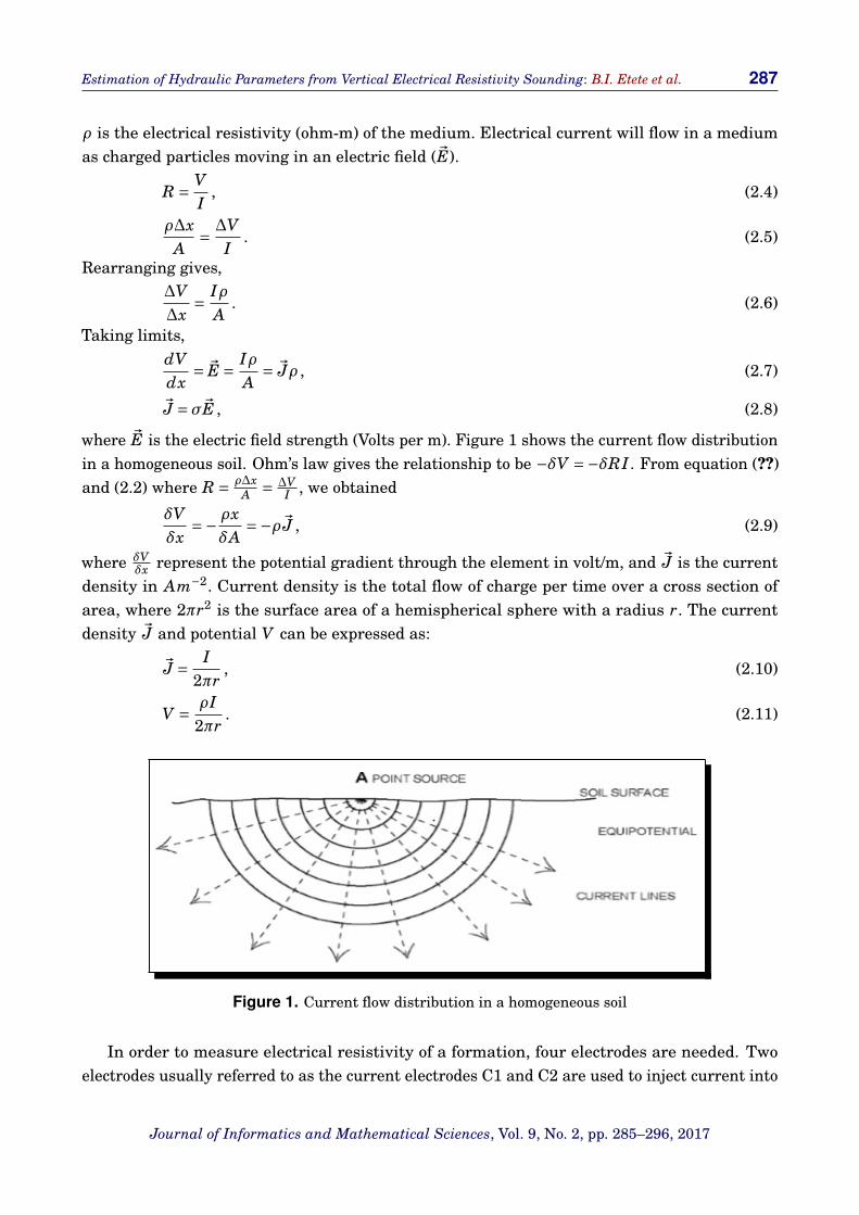
where ~E is the electric field strength (Volts per m). Figure 1 shows the current flow distributionin a homogeneous soil. Ohm’s law gives the relationship to be −δV =−δRI . From equation (??)and (2.2) where R = ρ∆x

A = ∆VI , we obtained

δVδx

=− ρxδA

=−ρ~J , (2.9)

where δVδx represent the potential gradient through the element in volt/m, and ~J is the current

density in Am−2. Current density is the total flow of charge per time over a cross section ofarea, where 2πr2 is the surface area of a hemispherical sphere with a radius r. The currentdensity ~J and potential V can be expressed as:

~J = I2πr

, (2.10)

V = ρI2πr

. (2.11)

Figure 1. Current flow distribution in a homogeneous soil

In order to measure electrical resistivity of a formation, four electrodes are needed. Twoelectrodes usually referred to as the current electrodes C1 and C2 are used to inject current into



the ground while the other two electrodes (potential electrodes) P1 and P2 are used to recordthe resulting potential difference (∆V ). The equation is given as:

∆V =∆VP1 −VP2 , (2.12)

∆V = ρI2π

[1

rc1p1− 1

rc2p1− 1

rc1p2+ 1

rc2p2

], (2.13)

where rc1p1, rc1p2, rc1p2 and rc2p2 are the geometrical distance between the electrodes and theelectrical resistivity can be calculated using:

ρ = 2π

1rc1p1

− 1rc2p1

− 1rc1p2

+ 1rc2p2

, (2.14)

ρ = ∆VIG

. (2.15)

G is a geometrical factor and it depends on the electrode configuration.

3. Materials and Methods3.1 Electrode ConfigurationThe configuration used for the measurements of vertical electrical sounding (VES) data was theSchlumberger electrode configuration. The electrode configuration for Schlumberger array isshown in Figure 2.

Figure 2. Schlumberger electrode configuration

In Figure 2, 2l is the spacing between the inner potential electrodes P1 and P2, while 2Lis the spacing between the current electrodes C1 and C2. From the configuration above theapparent resistivity is given as:

ρa =π× VI

[(AB/2)2 − (MN/2)2

MN

], (3.1)

K = πl2

2l, (3.2)

ρa = K∆V

I, (3.3)



where ρa is the apparent resistivity and K is the geometric factor, which depends on thegeometry or arrangements of the four electrodes. The apparent resistivity obtained from thevarious VES points can be used to estimate the true resistivities of various layers (lithologies)delineated about the point investigated.

3.2 Data Collection and ProcessingVertical electrical sounding (VES) using the Schlumberger configuration was conducted at thirtylocations in the study area. The equipment used to take the measurement in this survey wasthe ABEM Terrameter (it displays the apparent resistivity value). A 12V DC power source wasused to power the Terrameter. The four electrodes were inserted into the ground following theSchlumberger configuration. The potential difference at each progressive point (AB/2) wheremeasured and displayed on the ABEM Terrameter and then they were recorded and saved.The various apparent resistivities obtained from the vertical electrical sounding were plottedagainst the corresponding values for AB/2 using a log-log graph to give a sounding curve. Thesounding curve obtained from the plot between the apparent resistivity values and then AB/2was matched against the theoretical master curve to get an initial model for the interpretation.The model obtained from the curve matching was used as an initial input model for the computeriteration. The software used for the iteration is the WIN RESIST software.

3.3 Hydraulic Parameters EstimationWater samples were collected from different borehole points in Iyesi where thirty VES datawere collected. The conductivity measurements for the water samples were conducted usinga 4510 conductivity meter. From the conductivity values obtained for the water samples, theresistivity ρ which is the inverse of conductivity σ can be obtained from the water samples.

ρ = 1σ

(3.4)

From Archie’s (1942, 1950) equation for electrical resistivity ρ,

ρ = aρwφ−m , (3.5)

F = ρ f

ρw, (3.6)

where F is the formation factor, ρ f is the resistivity of formation, ρw is the resistivity of water,ρw is the tortuosity (a ≈ 1, for unconsolidated sediments), m is cementation exponent and φ isporosity. The cementation exponent ranges between 1.8 and 2.0, for consolidated sandstones,and 1.1 and 1.3 for unconsolidated clean sands.

F = aφ−m . (3.7)

The porosity φ of the formation can be estimation using the value obtained from the formationfactors. The water saturation Sw can be accounted for in Archie’s law as follows:

Fi = ρ

ρw= aφ−mS−n

w (3.8)



Equation (3.8) is known as the generalized Archie’s second law, where exponent n is thesaturation index, usually equal to 2. Using the Kozeny-Carmen-Bear equation (Carmen [5];Kozeny [11]), the hydraulic conductivity K can be calculated given:

K =(δw gµ

)(d2

180

)[φ3(

1−φ)2

](3.9)

where δw is the fluid density (1000 kg/m3), µ is the dynamic viscosity of water (0.0014 kg/ms), gis acceleration due to gravity (9.81 m/s2) and d is the grain size. The unit of K is m/sec. Theintrinsic permeability k f of the aquifer is given as:

k f =d2

180φ3

(1−φ)2 . (3.10)

Thus, the intrinsic permeability and hydraulic conductivity can be related using equation(Nutting, 1930) so that

K = δw gµ

k f . (3.11)

Using the relationship between the hydraulic conductivity K and the thickness b thetransmissivity of the aquifer is given as

T = Kb . (3.12)

Using the relationship between the hydraulic conductivity K and electrical resistivity ρ of anaquifer, the transmissivity of the aquifer is given

T = (Kρ)S , (3.13)

where ρ is the bulk resistivity and S is the longitudinal unit conductance of the aquifer materialwith thickness b given by b/ρ. For a lateral hydraulic flow and current flowing transversely, thetransmissivity of the aquifer becomes

T = (K /ρ)R , (3.14)

where R is the transverse unit resistance of the aquifer material given by bρ. If the aquiferis saturated with water with uniform resistivity, then the product Kρ or K /ρ would remainconstant. The above equations may therefore be written as T =αS; α= Kρ and T =βR, β= K /ρwhere α and β are constants of proportionality.

4. ResultsThe geoelectric parameters obtained from the VES data interpretation for this work arepresented in Tables 1 and 2. The results obtained from the water samples collected within thestudy area were used to obtain the hydraulic conductivity values. Table 3 shows the valuesobtained for the hydraulic conductivity, porosity, formation factor, transmissivity, permeability,longitudinal conductance and transverse resistance. The thickness and resistivity of the aquiferwere obtained from the inverse model of the resistivity soundings while the formation factorand porosity were obtained using Archie’s law.



Table 1. Table showing the VES correlation of the layer models obtained from the apparent resistivityand their lithologies

Table 2. Table showing the VES correlation of the layer models obtained from the apparent



Table 3. Table showing aquifer geologic properties for VES data

4.1 Geoelectric ParametersThe subsurface comprises of different lithologies which are sandy clay, lateritic clay, silty clay,silty sand, mudstone (confining bed), fine-to-medium grain sand, coarse sand and clayey mud.From Tables 1 and 2, the resistivity of the top soil varies from 22.5Ωm to 321.9Ωm; thethickness ranges from 0.9 m to 2.1 m. The resistivity of the top soil depends on clay volume,moisture content and degree of compaction. The resistivity of the underlying geoelectric layerranges from 39.2Ωm to 979.0Ωm with thickness ranging from 2.2 m to 16 m. The third layeris an intercalation of silt and clay and has its thickness and resistivity shown in Table 1 andTable 2. The fourth geoelectric layer, an intercalation of silt and sand, was delineated. Theresistivity ranges from 831.9Ωm to 2655.3Ωm; the thickness ranges from 4.1 m to 33.3 m.Underlying this geoelectric layer is a very high resistive substratum with resistivity rangingfrom and thickness ranging between 1669.0Ωm to 10259.1Ωm and 15.4 m to 41.7 m.

The sixth layer (medium grain sand) which is also an aquifer unit is overlain by theconfining bed (mudstone) which is characterized by its high resistive unit. The sixth layer hasits resistivity ranging from 348.4Ωm to 784.0Ωm (Figure 4) and thickness ranging from 12.1 mto 16.1 m (Figure 5). Mudstone is a mix of silt and clay sized particles. It contains phosphateparticle which is also responsible for its high resistivity value. The seventh geoelectric layerdelineates the major aquifer which consists of unconsolidated coarse grain sands. Underlyingthe major aquifer is a low resistive layer ranging from 35.5Ωm to 236.6Ωm.



(a)

(a)

(b)

(b)

(c)

(c)

(d)

(d)

(e)

(e)

(f)

(f)

Figure 3. Representative of the iterated VES curves showing the inverse models of the geoelectricalparameters for (a) VES 1, (b) VES 2, (c) VES 3, (d) VES 4 (e) VES 5, (f) VES 6

4.2 Parameter EstimationThe hydraulic properties (hydraulic conductivity and transmissivity) and Dar’Zarrouk’sparameters (longitudinal conductance and transverse resistance) are computed from thegeoelectric parameters of the aquifer Table 3. Following the determination of the mostappropriate values of the tortuosity parameter (α) and cementation factor (m) 1 and 1.3,respectively, the hydraulic parameters of the aquifer were calculated for all locations. Theseparameters i.e. (m) and (α) are essential to estimate an aquifer hydraulic parameters usinggeoelectrical resistivity. The longitudinal conductance of the major aquifer is generally lowranging from 0.07723Ω−1 to 0.12440Ω−1. The transmissivity in this area is generally high witha porosity range of 18 percent to 27 percent with an average of 22 percent and is spatiallyrelated to the hydraulic conductivity. This indicates a confined aquifer and is also characterized



Resistivity

Latitude

Lo

ngi

tud

e

Figure 4. Iso-resistivity map of the aquifer.

Longitude

L

ati

tu

Figure 5. Representation of the aquifers thickness

with high hydraulic conductivity as indicated in the table above. The transverse resistance ofan aquifer increases with increasing transmissivity and yield. The transverse resistance rangesfrom 1443.60Ωm2 to 2452Ωm2. This range indicates a high value of transmissivity and yield ofthe major aquifer in the study area.



5. DiscussionsThe direction of groundwater flow follows a curved path through an aquifer from areas of highwater levels to areas of low water levels; that is from recharge areas to discharge points invalleys or seas. It is therefore necessary to know the direction of groundwater flow and takesteps to ensure that land use activities in the recharge area will not pose a threat to the qualityof the groundwater (Freeze and Cherry [9]). Hence, the direction of flow Figure 6 was generatedusing the surfer 8 software.

Latitude

Lo

ngi

tud

e

Depth

Figure 6. Map showing the groundwater flow in the subsurface

6. ConclusionsGeoelectrical resistivity survey was carried out in Iyesi, Ota, Ogun state, southwesternNigeria. The aim of the survey was to assess the groundwater resource potential in the area.The information of groundwater resource potential is fundamental for groundwater resourceimprovement, administration and monitoring. The results of this study show that the depthto aquifer in the study area ranges from −23.6 m to 19.6 m. The aquifer unit show appreciablethickness that can support adequate drawdown for groundwater extraction. The porosity,hydraulic conductivity and transmissivity values indicate high productivity and high yield forthe aquifer unit. It is recommended that boreholes within the study area should be drilled to aminimum depth of about 47 m (144 ft) to ensure adequate draw-down and perennial yield. Also,better planning, development and management of the groundwater resources.



Acknowledgment

The authors appreciate Covenant University for partial sponsorship.

Competing InterestsThe authors declare that they have no competing interests.

Authors’ ContributionsAll the authors contributed significantly in writing this article. The authors read and approvedthe final manuscript.

References[1] G. Archie, The electrical resistivity log as an aid in determining some reservoir characteristics,

Petroleum transactions of the American Institute of Mineralogical and Engineers 146 (1942), 54 –62.

[2] G. Archie, Introduction to petrophysics of reservoir rocks, American Association of PetroleumGeologists Bulletin s (1950), 943 – 961.

[3] J.J. Breusse, Modern geophysical methods for subsurface water exploration, Geophysics 28 (1963),633 – 657.

[4] D.C. Carmen, Fluid flow through a granular bed, Transaction Institute of Chemical Engineering 15(1937), 150 – 157.

[5] D.C. Carmen, Flow of Gases through Porous Media, Academic Press, New York (1956), 182 p.

[6] European Association of Exploration Geophysicists, Compagnie Generale de Geophysique, Mastercurves for electrical sounding, 2nd revised edition (1963), https://books.google.co.in/books/about/Master_Curves_for_Electrical_Sounding.html?id=g1BmPAAACAAJ&redir_esc=y.

[7] M.B. Dobrin, Introduction to Geophysical Prospecting, 2nd edition, McGrow-Hill, New York (1960),446 p.

[8] R.A. Freeze and J.A. Cherry, Groundwater, Prentice Hall Inc., Englewood Cliffs, New Jersey (1979),7 p.

[9] A. Ginzburg, Resistivity surveying, Geophysical Surveys 1 (1974), 325 – 355.

[10] J. Kozeny, Ueber kapillare leitung des wassers im boden, Sitzungsberichte Akademie derWissenschaften Wien 136 (1927), 271 – 306.

[11] J. Kozeny, Hydraulics, Springer, Vienna (1953), 546 – 549.

[12] P.G. Nutting, Physical analysis of oil sands, American Association of Petroleum Geologist Bulletin14 (1930), 1337 – 1349.


https://books.google.co.in/books/about/Master_Curves_for_Electrical_Sounding.html?id=g1BmPAAACAAJ&redir_esc=y

https://books.google.co.in/books/about/Master_Curves_for_Electrical_Sounding.html?id=g1BmPAAACAAJ&redir_esc=y

estimation of hydraulic parameters from vertical

Documents