new directions in time-resolved neutron diffraction...
TRANSCRIPT
Glasgow Theses Service http://theses.gla.ac.uk/
Boscaino, Annalisa (2014) New directions in time-resolved neutron diffraction: probing high power microwave materials synthesis in situ. PhD thesis. http://theses.gla.ac.uk/5699/ Copyright and moral rights for this thesis are retained by the author A copy can be downloaded for personal non-commercial research or study, without prior permission or charge This thesis cannot be reproduced or quoted extensively from without first obtaining permission in writing from the Author The content must not be changed in any way or sold commercially in any format or medium without the formal permission of the Author When referring to this work, full bibliographic details including the author, title, awarding institution and date of the thesis must be given

NEW DIRECTIONS IN TIME-RESOLVED
NEUTRON DIFFRACTION.
PROBING HIGH POWER MICROWAVE
MATERIALS SYNTHESIS IN SITU
By
Annalisa Boscaino
Submitted in the fulfilment of the requirements for the
Degree of Doctor of Philosophy
School of Chemistry
University of Glasgow
October 2014

1
Abstract
This thesis aims to describe the design, implementation and use of a novel
instrumental set-up which, by providing in situ ultra-rapid synthesis of
transition metal carbides, is capable of investigating their reaction
mechanisms, thus developing new procedures to reduce energy demanding
industrial processes.
Ultra-rapid synthesis of titanium carbide, TiC - the main binary system
studied - has been achieved through the development of a reproducible
experimental technique and an investigation into crucial reaction
variables, microwave applicators and applied power. Specifically in the
case of the single mode cavity, this resulted in the completion of the
majority of reactions within 60 s.
TiC formation started from its elemental precursors (titanium and
graphite). An attempt to produce TiC by using a domestic microwave oven
successfully lead to the synthesis of the product after ca. 15 minutes.
A further achievement was made by exploiting the linear relationship
between the expansion of graphite (increase of c parameter) with
temperature, which allowed for in situ bulk temperature measurements
crystallographically. This method of measurement represents a more
reliable alternative to traditional techniques (i.e., pyrometery or use of
thermocouples).
The majority of this work was performed on the D20 beam line at the ILL
neutron source facility, in Grenoble. The choice of this beam line, capable

2
of collecting diffractograms at high speed rate was crucial for revealing
the reaction pathways of TiC MW-promoted synthesis, for the first time.
Raman spectroscopy and scanning electron microscopy techniques were
used in an effort to establish the presence of any amorphous phases in the
system.
The same methodology was applied in preliminary experiments to other
ternary transition metal-carbon systems. In particular, tungsten (W) and
tantalum (Ta) compounds were investigated, starting from both the
elements and respective oxides, WO2 and Ta2O5.

3
Acknowledgments
First of all, I would like to thank my two supervisors, Professor Duncan H.
Gregory and Dr. Thomas C. Hansen for their assistance and help during
my PhD. A warm thank to Alain Daramsy, D20 technician, who helped
this thesis to evolve from the experimental point of view, with his
expertise and patience. I also would like to thank Jennifer Kennedy and
Helen Kitchen for their help. In particular, Jen thanks for all the helpful
discussion and support, which I really appreciate.
Dr. Timothy D. Drysdale and Dr. A. Gavin Whittaker were very helpful
and present.
A special thank to Marco, Rei and Morgan, with their joy and love they
are my precious supporting team.

4
List of Contents
Abstract 1
Acknowledgements 3
List of Contents 4
List of Acronyms 6
List of Figures and Tables 7
Chapter 1: Introduction 15
1.1 Microwave Radiation 16
1.2 History of Microwave Processing 17
1.3 Microwave Interaction with Dielectric Materials 23
1.3.1 The Microwave Effect 28
1.4 Microwave-Induced Synthesis of Ceramics: Binary and Ternary
Carbides 32
1.4.1 Titanium Carbide 32
1.4.2 Other Ternary Compounds 35
1.5 Role of in situ Neutron Powder Diffraction in Microwave
Processing of Carbides and Aim of This Thesis 39
References 40
Chapter 2: Experimental Theory and Methods 47
2.1 Microwave radiation and instrumentation 47
2.1.1 Microwave Instrumentation for Single Mode Cavity
(SMC) and Multi Mode Cavity (MMC) 54
2.1.2 Temperature Measurements 67
2.2 Synthesis and Processing 70
2.2.1 Synthesis using a multi mode cavity (MMC) 71
2.2.2 Synthesis using a single mode cavity (SMC) 72
2.3 Physical methods to characterize solids 74
2.3.1 Basic Concepts of Crystallography 76
2.3.2 Neutron Scattering and Powder Neutron Diffraction 84
2.3.3 Powder X-Ray Diffraction 93
2.3.4 Rietveld refinement and Sequential refinement strategy 97
2.3.5 Raman Spectroscopy 104
2.3.6 Scanning Electron Microscopy (SEM) 111
References 115
Chapter 3: Design and Implementation of the in-situ Reactor 118
3.1 Introduction 118
3.2 Step one. Design of MW set-up and reactor on D20 119
3.3 Step two. Remote control 131
References 132
Chapter 4: Microwave Studies in the Ti-C System 134

5
4.1 Single and Multi Mode Cavity Synthesis in the Ti-C system 134
4.1.1. MW synthesis in the Ti-C system and experimental
details 136
4.2 Results 141
4.2.1 MMC microwave studies of Ti-C system 143
4.2.1.1 Sample 1. Synthesis of TiC starting from Ti + C 143
4.2.2 SMC microwave studies of the TiC system 144
4.2.2.1 Sample 2. SMC synthesis using the Gaerling reactor 144
4.2.2.2 In situ synthesis in Sairem reactor. Two cases 144
4.2.2.3 Rietveld refinement 148
4.2.2.4 Temperature measurement 155
4.2.2.5 SEM 160
4.2.2.6 Raman spectroscopy 163
4.3 Discussion and Conclusion 166
4.4 Preliminary results on other binary and ternary systems and future
studies 171
4.4.1 Experimental details 172
4.4.2 Preliminary results 174
4.4.2.1 Ti-Ta-C 174
4.4.2.2 Ti-W-C 176
4.4.2.3 Ti-WO2-C 177
4.4.2.4 Ti-Ta2O5-C 178
4.4.3 Discussion and Conclusion 179
References 180
Chapter 5: Conclusions 183

6
List of Acronyms
MW Microwaves
UHF Ultra High Frequency
SHF Super High Frequency
EHF Extremely High Frequency
DMO Domestic MW Oven
E Electric field
FP Forward Power
RP Reflected Power
TWT(s) High-power Travelling WaveTube(s)
TE Transverse Electric
TM Transverse Magnetic
TEM Transverse Electromagnetic
MMC Multi Mode Cavity
SMC Single Mode Cavity
PND Powder Neutron Diffraction
XRD X-Ray Diffraction
SEM Scanning Electron Microscope
PXD Powder X-Ray Diffraction
*Other abbreviations not shown here will be explained in the relevant
chapters

7
List of Figures and Tables
Figure 1.1. Location of the MW frequency band in the electromagnetic
spectrum and band designation. It is generally between 1 – 60 GHz that
MWs find their application in a variety of areas, while for the MW
processing of materials the S-band (between 2 – 4 GHz) is the most
exploited. 16
Figure 1.2 Resonant-cavity magnetron. In vacuum tubes, the anode is at a
higher potential than the cathode: this leads to a strong electric field and
the cathode is heated to remove the valence electrons. Once removed,
electrons are accelerated toward the anode by the electric field. An
external magnet is used to generate a magnetic field orthogonal to the
electric one and the magnetic field creates a circumferential force in the
electron as it is accelerated to the anode. This force causes the electron to
travel in a spiral direction, creating a swirling cloud of electrons. As
electrons pass the resonant cavities, the cavities set up oscillations in the
electron cloud, and the frequency of the oscillation depends on the size of
the cavity. 18
Figure 1.3 An example of how MW irradiation can drastically reduce
reaction times in organic reactions, by superheating the solvents up to 18 –
69 °C. All these reactions were performed at 560W - with the exception of
the 1-pentanol case, at 630W - in a DMSO. 21
Figure 1.4 The inverse temperature profile in MW heating. 24
Figure 2.1. a) Schematic of two charged plates (electrodes) without
applying an external electric field. b) The polarization of the dielectric
produces an electric field opposing the field of the charges of the plates.
The dielectric acts as a capacitor, allowing charge to be stored. As
consequence, no conductivity is observed between the two plates. (Picture
adapted from: http://hyperphysics.phy-
astr.gsu.edu/hbase/electric/dielec.html). 48
Figure 2.2 (a) H2O molecules showing a permanent dipole. (b) Permanent
dipoles are usually represented by an arrow. (c) In thermal equilibrium,
dipoles are randomly arranged. The dipole moments from different
molecules cancel out and the net polarization is zero. (d) When applying
an external electric field, dipoles rotate in order to align with the field E
and with each other: the net polarization is therefore non-zero. 49
Figure 2.3 Very similar to dipolar polarization, ionic polarization occurs
in crystals under external field E. 49

8
Figure 2.4 In the case of noble gases, dielectric heating occurs when its
electron cloud has been shifted by the influence of an external charge, and
it is not centered on the nucleus. 50
Figure 2.5 Materials are grouped into three categories (from left to right):
MW transmitters; MW reflectors, and MW absorbers. 53
Figure 2.6 Difference between conventional and MW heating. A
wavefront is the surface of points of the radio wave having the same
phase. 54
Figure 2.7 a) Schematic diagram of the magnetron tube: top view (left);
side view (right), as in reference [7]. b) Scheme of a DMO magnetron (as
in reference [8]). 55
Figure 2.8 a) A DMO magnetron section (Picture taken from
http://www.microwaves101.com/encyclopedia/magnetron.cfm). b) A
Sairem® 2 kW magnetron section (this magnetron has been used in the
thesis: the ceramic protection of the antenna has been broken by an arc,
which occurred during experiments). 56
Figure 2.9 TWT, as in reference [7], consisting of two main components:
an electron gun and a helical transmission line. Because there are no
resonant structures, TWT can amplify a large variation of frequencies
(bandwidth) within the same tube. The heated cathode emits a stream of
electrons that is accelerated toward the anode, and the electron stream is
focused by an external magnetic field. The purpose of the helix is to slow
the phase velocity of the MW (the velocity in the axial direction of the
helix) to a velocity approximately equal to the velocity of the electron
beam. For amplification of the signal to occur, the velocity of the electron
beam should be just faster than the phase velocity of the helix. In this case,
more electrons are being decelerated than accelerated, and the signal is
amplified because energy is being transferred from the electron beam to
the MW field. 57
Figure 2.10 a) TE (transverse electric) and TM (transverse magnetic)
mode. (Picture from:
http://www.allaboutcircuits.com/vol_2/chpt_14/8.html); b) TEM mode
waveguide: both field planes (electrical and magnetic) are perpendicular
(transverse) to the direction of signal propagation. 59
Figure 2.11 Scheme of a rectangular waveguide, in Cartesian coordinate
system (left). Scheme of a circular (or cylindrical) waveguide of radius a,
in cylindrical coordinate system. In both cases, the waveguide is
positioned with the longitudinal direction along the z-axis. 60

9
Table 2.2 Values for pmn cylindrical waveguides
(http://www.rfcafe.com/references/electrical/waveguide.htm). 63
Figure 2.12 a) Photographic and b) schematic representation of the TE10n
MW heating cavity. 66
Figure 2.13. Schematic of a SMC MW device, suitable for material
processing comprising a power supply; magnetron; rectangular
waveguide; 3-port ferrite circulator; quartz window (for preventing plasma
discharge destroying the magnetron); tuner; waveguide; applicator
(cylindrical or rectangular); short circuit (or metal plate).
It is difficult to heat ceramics with a domestic microwave oven (MMC),
because ” for ceramics is extremely small compared to that, for example,
of food. (The MMC type is suitable for heating of materials of
comparatively large ”, and the SMC type is suitable for that of small ”)
[15]. 66
Figure 2.14 Schematic of a pyrometer. An optical system collects the
visible and infrared energy from an object and focuses it on a detector.
The detector converts the collected energy into an electrical signal to drive
a temperature display or control unit. The detector receives the photon
energy from the optical system and converts it into an electrical signal.
Two types of detectors are used: thermal (thermopile) and photon
(photomultiplier tubes). Photon detectors are much faster than the
thermopile type. This enables the user to adopt the photon type for
measuring the temperature of small objects moving at high speed. (Picture
taken from: http://www.globalspec.com/reference/10956/179909/chapter-
7-temperature-measurement-radiation-pyrometers). 69
Figure 2.15. a) Picture of the MMC used in the work described in this
thesis; a) Schematic of silica beaker plus sample holder (quartz tube). 72
Figure 2.16 a) MW system used at Glasgow University; b) Cylindrical
applicator – with a choke for pyrometer readings; c) TiC reaction under
MW irradiation, in act. 74
Figure 2.17 a) Single mode MW device, on two-axis diffractometer D20,
at ILL. On the power supply display, FP and RP can be read. A MW
leakage detector has been installed. b) The single mode cylindrical
applicator has been designed specifically for D20. Its design addresses
multiple issues, such as avoiding interference with both the sample and the
neutron beam, complying with instrument geometry constraints and
avoiding activation risks. 75

10
Figure 2.18 a, b, and c and the angles between them ( , between axes b
and c; , between axes a and c and , between axes a and b) describe the
unit cell. 77
Figure 2.19 The seven crystal systems, listed in order of decreasing
symmetry. a) Cubic (a=b=c, ; b) Hexagonal (a=b≠c,
; c) Tetragonal (a=b≠c and = ; d) Trigonal
(a=b≠c, or alternative setting for the special case of
rhombohedral lattice, a=b=c, ≠ ; d) Orthorhombic (a≠b≠c,
; e) Monoclinic (a≠b≠c, ≠ ; f) Triclinic (a≠b≠c,
≠ ≠ ≠ . 77
Table 2.3 Symmetry elements. 78
Table 2.4 The essential symmetry for the seven crystal systems. 79
Figure 2.20 The fourteen Bravais lattice (Picture from:
http://www.seas.upenn.edu/~chem101/sschem/solidstatechem.html). 80
Figure 2.21 Translational symmetry operations: 41screw axis (a) and c
glide plane (b). Screw 41is obtained by a 2 /4 rotation around z axis,
combined with a c/4 sliding along z axis. Glide plane c means a reflection
perpendicular to y axis with a c/2 sliding along z axis. 80
Figure 2.22 The Bragg condition for the reflection of X-rays by a crystal.
X-ray crystallography relies on the fact that the distances between atoms
in crystals are of the same order of magnitude as the wavelength of X-rays
(1 Å). Hence a crystal acts as a three-dimensional diffraction grating to a
beam of X-rays. The resulting diffraction pattern can be interpreted to give
an insight into the crystal structure of the sample produced. 83
Figure 2.23 A beam of thermal neutrons incident on a sample. 84
Figure 2.24 Scattering process of a neutron beam by a sample is described
in terms of polar coordinates. 84
Figure 2.25 A spherical wave is used for describing a scattered neutron. b
is the scattering length, experimentally determined, characteristic of the
nucleus. 90
Figure 2.26 Schematic of 2-axis diffractometer D20, at the Institut Laue-
Langevin (Picture from:http://www.ill.eu/instruments-
support/instrumentsgroups/instruments/d20/description/instrument-
layout/). 93

11
Figure 2.27 Bragg-Brentano geometry. Sample holder is in position “S”.
In black, collimators (Picture taken from:[5]). 96
Figure 2.28 Spectroscopic transitions underlying several types of
vibrational spectroscopy. The arrow line thickness is about proportional to
the signal strength from the different transitions. 106
Figure 2.29 Raman spectra of commercially available TiC
(as in ref:[37]). 110
Figure 2.30 General set-up of a SEM microscope. 112
Figure 3.1. Final shape of the applicator (AutoCAD drawing): 80 mm
diameter and 352 mm length. It responds to multiple problems, such as
avoiding interference with both the sample and the neutron beam, fitting
D20 geometry constraints and does not exhibit permanent neutron
activation on exposure to the beam. 120
Figure 3.2 (a) 3D image of the applicator (and 90° bend waveguide); (b)
Plot of the electric field magnitude. Red spots indicate the position of the
maxima of the electromagnetic field inside the cylindrical reactor. These
are also the positions where the maximum MW/sample coupling can be
found. 122
Figure 3.3. (a) First MW set-up used on D20. It shows two bend
waveguides (after the isolator and before the transition waveguide). (b)
Diagram of the first MW set-up. (c) Second configuration of the set-up, on
D20. The first bend waveguide (after the isolator) has been removed. Both
solutions were unable to transfer the necessary power into the applicator
and at the sample position. 126
Figure 3.4. (a) Working MW set-up, mounted on D20: (1) MW generator
and magnetron; (2) isolator (3-port ferrite circulator); (3) quartz window;
(4) 3-stub tuner; (5) transition waveguide; (6) cylindrical applicator; (7)
power supply; (8) MW survey meter. (b) Schematic of MW set-up. 128
Figure 3.5. (a) MW-SMC set up mounted on the D20 beam line and a
zoom of the reaction tube (highlighted in yellow); (b) reaction tube loaded
into the applicator. This configuration allows manual adjustment of the
position of the sample in the cavity, thus achieving the best MW/sample
coupling position (namely, where the difference between FP and RP takes
its maximum value). 129
Figure 3.6. Schematic of the reaction tube (right), inside the applicator.
The quartz wool is needed for supporting the pellet in the quartz tube.
Quartz wool is inert for both neutrons and sample, it does not contribute

12
significantly to the diffraction pattern and it does not burn at the
temperature reached in the experiments. 130
Figure 3.7. (a) The microcontroller table moves the MW set-up vertically
(y-axis – maximum run 30 cm), horizontally (x-axis – maximum run 30
cm) and on the detector plane ( angle – 180° degrees), in order to allow
the best centering position of the sample in the neutron beam, after the
best coupling position MW/sample has been found; (b) Example of
microcontroller table shifted on the plane by 45° in respect to the
position in figure 3.7(a). 131
Figure 4.1 (a) Gaerling set-up, as used in GU for Ti-C system synthesis
experiments. (b) Cylindrical TE10n SMC in the Gaerling set-up. The
reaction tube is placed vertically in this cavity, from the (open) top. The
choke (indicated by a black arrow) is used for temperature readings (via
pyrometer). (c) Schematic of Gaerling set-up. 141
Table 4.1 Summary of the experimental conditions for samples 1-4. 142
Figure 4.2 Sample 1. Single phase TiC after 10 min of MW irradiation in
an MMC, in air. The graphite (002) peak is also indicated (○). 143
Figure 4.3 Sample 2. Single phase TiC after 10 min of MW irradiation in
Gaerling SMC reactor, in air. The graphite (002) peak is also indicated
(○). 144
Figure 4.4 Full reaction diffraction profile for sample 3. The shift of the
carbon peaks to lower 2 angles (at ca. 50 s) is a good indicator of a rapid
temperature increase. The formation of TiC (around 100 s) is revealed by
new peaks appearing at ca. 31° and 63° 2 . In this reaction, TiC is not
formed as a pure phase, as -Ti is always detectable and present until the
end of reaction. 145
Figure 4.5 Sample 3. For clarity, the diffractograms have been normalized
at 0, 10, 60, 100, and 120 s by shifting their intensity and adding a
constant of, respectively, 0, 500, 1000, 1500, 2000. 146
Figure 4.6. Full reaction diffraction profile for sample 4. The formation of
TiC (~ 50 s) is indicated by new peaks appearing at ca. 36 ° and
72 ° 2 . 147
Figure 4.7 Sample 4. As in Fig. 4.7, for clarity, diffractograms have been
normalised at 0, 10, 20, 50, and 90 s by shifting their intensity and adding
a constant of, respectively, 0, 500, 1000, 1500, 2000. Reflections from -
Ti (□), C (○), -Ti (*), and TiC (♦) are indicated. 148

13
Table 4.2 Crystallographic data from Rietveld refinement for samples 1,
2, 3 and 4. 150
Figure 4.8 Profile plot for Rietveld refinement against PXD data, for
sample 1 (MMC, 10 min, 800 W). The pattern is dominated by five peaks
that match with the reflections from the (111), (200), (220), (311) and
(222) planes of the cubic structure of TiC. 151
Figure 4.9 Profile plot for Rietveld refinement against PXD data, for
sample 2 (SMC, Gaerling set up, 10 min, 1 kW). As for Fig. 4.8, the
pattern is dominated by five peaks that match with the reflections from the
(111), (200), (220), (311) and (222) planes of the cubic structure of
titanium carbide. 152
Figure 4.10 (a) Profile plots for Rietveld refinement against neutron data
for sample 3, (a) at t = 0; (b) at t = 60 s; (c) at t = 100 s; (d) at t = 120 s.
Reflections from C (○) are indicated. 154
Figure 4.11 (a) Profile plots for Rietveld refinement against neutron data
for sample 4, (a) at t = 0. (b) at t = 20 s. (c) at t = 90 s (end of
reaction). 155
Figure 4.12 Reaction temperature vs reaction time for sample 3. -Ti
appears at higher temperature than conventional furnace case (1253 K and
1156 K [1], respectively). The experimental T at which the presence of
TiC phase is firstly observed in the diffraction pattern is 1370 K. After the
appearance of TiC, the temperature increases to a maximum of 1396 K
after ca. 120 s of MW irradiation, and begins to slowly decrease beyond
this time. 158
Table 4.3 Data for Fig. 4.12 (where reaction temperature vs reaction time
is plotted, for sample 3). 159
Figure 4.13 Reaction temperature vs reaction time for sample 4.The
phase transition occurs after ~20 s, at a much lower temperature (648 K)
than both sample 3 and conventional furnace. The experimental T at which
the presence of TiC phase is firstly observed in the diffraction pattern is
1322 K. After the appearance of TiC, the temperature increases up to a
maximum of 1603 K (after ca. ~70 s of MW irradiation), and slowly
decreases thereafter. 159
Table 4.4 Data for Fig. 4.13 (where reaction temperature vs reaction time
for sample 4). 160

14
Figure 4.14 (a) SEM picture (20 m) for sample 2 (SMC, Gaerling set-up,
1 kW, 10 min process); (b) SEM picture (20 m) for sample 3 (Sairem set-
up, 0.500 kW); (c) SEM picture (20 m) for sample 4 (Sairem set-up,
0.500 kW). 162
Figure 4.15 SEM images of sample 1 (MMC, 800 W). 163
Figure 4.16 (a) Raman spectra (literature data) taken from different
particles of commercially available graphite [2]. (b) Raman spectra
(literature data) of commercially available TiC powder (Aldrich, purity of
98%) [2], taken from seven different particles. 164
Figure 4.17 Raman spectrum for sample 1(MMC, 800 W). 165
Figure 4.18 Multiplot of Raman spectra for sample 3, collected from
different region of the same sample (SMC, 500 W). 165
Figure 4.19 Multiplot of Raman spectra for sample 4, collected from
different regions of the same sample (SMC, 500 W). 166
Figure 4.20 Time-temperature plot for the conventional solid state
reaction of Ti + C, as reported by Winkler et al. [1]. 168
Figure 4.21 Phase fraction in sample 3. Although the -Ti concentration
slowly decreases, it never disappears and always coexists with TiC. 169
Figure 4.22 Phase fraction vs reaction time for -Ti (blue), -Ti (red) and
TiC (green), in the SMC synthesis of sample 4. 170
Table 4.5. All the systems processed by means of in situ MWs, in Sairem
set-up, at ILL. Stoichiometric ratios were chosen in order to observe the
role (i.e., on the speed and the nature of product formation) of different
concentration of Ti in the mixture. 174
Figure 4.23. Diffractograms for Ti(1-x)TaxCy system (x=0.1-0.9, x = 0.1
and y=2). From the bottom, in black, TaTiC (1:1:2 ratio); in red,
Ti0.1Ta0.9C2; in green, Ti0.2Ta0.8C2; in blue, Ti0.3Ta0.7C2; in yellow,
Ti0.4Ta0.6C2 ; in turquoise Ti0.5Ta0.5C2; in pink, Ti0.6Ta0.4C2; in dark green,
Ti0.7Ta0.3C2 ; in orange, Ti0.8Ta0.2C2 ; and in violet Ti0.9Ta0.1C2. For
comparison, MW-processed TiC (in cyan) has been reported (sample 4, as
described in Chapter 4). For clarity, diffractograms have been normalized
at 0, 10000, 20000, 30000, 40000, 50000, 60000, 70000, …, 100000 by
shifting their intensity and adding a constant of, respectively, 0, 10000,
20000, 30000, 40000, 50000, 60000, 70000, …, 100000. 175

15
Figure 4.24 Diffractograms for each of the mixture in the Ti(1-x)WxCy
system (x=0.1-0.9 x = 0.1 and y=1). Starting from the bottom, in black,
TiWC (1:1:1 ratio). Going upwards, Ti0.1W0.9C1 (in red), Ti0.2W0.8C1 (in
green), Ti0.3W0.7C1 (in blue), Ti0.4W0.6C1 (in maroon), Ti0.5W0.5C1 (in
turquoise), Ti0.6W0.4C1 (in pink), Ti0.7W0.3C1 (in dark green), Ti0.8W0.2C1
(in orange), Ti0.9W0.1C1 (in violet). Cyan line belongs to the MW-
processed TiC (as described in Chapter 4, sample 4). 176
Figure 4.25. Ti(1-x)(WO2)xCy with (x=0.3-0.9 x = 0.1) and (y=1). From
the bottom, Ti0.3(WO2)0.7C1 (in blue), Ti0.4(WO2)0.6C1 (in maroon),
Ti0.5(WO2)0.5C1 (in turquoise), Ti0.6(WO2)0.4C1 (in pink), Ti0.7(WO2)0.3C1
(in dark green), Ti0.8(WO2)0.2C1 (in orange), Ti0.9(WO2)0.1C1
(in violet). 177
Figure 4.26. Diffractograms for Ti(1-x)(Ta2O5)xCy system (x=0.6-0.9 x =
0.1 and y=2). From the bottom, Ti0.9(Ta2O5)0.1C2 (in pink),
Ti0.8(Ta2O5)0.2C2 (in green), Ti0.7(Ta2O5)0.3C2 (in blue), Ti0.6(Ta2O5)0.4C1 (in
yellow), Ti0.5(Ta2O5)0.5C2 (in turquoise), Ti0.4(Ta2O5)0.6C2 (in pink), and
Ti0.3(Ta2O5)0.7C2 (in dark green). 179

16
Chapter 1
Introduction
1.1 Microwave Radiation
Microwave (MW) energy is a non-ionizing electromagnetic radiation with
frequencies between 0.3 and 300 GHz, with wavelengths ranging from 1
m to 1 mm. This broad frequency region includes three bands: the ultra
high frequency, UHF, (300 MHz – 3 GHz); the super high frequency,
SHF, (3 – 30 GHz) and the extremely high frequency, EHF, (30 – 300
GHz) [1] (Fig 1.1).
Figure 1.1. Location of the MW frequency band in the electromagnetic spectrum and
band designation. It is generally between 1 – 60 GHz that MWs find their application in a
variety of areas, while for the MW processing of materials the S-band (between 2 – 4
GHz) is the most exploited1.
It has been proved that frequencies such as 6, 28, 35, and 94 GHz give
very uniform electric fields, allowing efficient MW/material coupling,
thus being preferred for MW processing [2, 3]. However, the US Federal
1 Picture adapted from: http://www.moatel.com/board/faq.html#top

17
Communication Commission (FCC) allocated 915 MHz (896 MHz in the
UK [4]), 2.45, 5.85, and 20.2-21.2 GHz for Industrial, Scientific, Medical
and Instrumentation applications (ISMI) [5-7], making other frequencies
unsuitable.
Moreover, despite the development in 2003 of a compact-size 5.8 GHz
magnetron by Kuwahara et al. [8], this frequency is not popular because of
high costs of devices [5], thus leading to 915 MHz and 2.45 GHz as the
two most used frequencies at laboratory scale [1, 9, 10].
1.2 History of Microwave Processing.
The history of MW processing starts in 1921, when Albert Hull developed
the first magnetron. At that time, he was studying diodes and the motion
of electrons in uniform electric and magnetic fields. He devoted particular
attention to understanding the special case of a system combining a
uniform and static magnetic field with a radial (i.e. perpendicular to
magnetic field lines) electric field [11]. Electrons moving in such a system
and the associated MW production are in fact the working principle of a
magnetron. Independently, other researchers worked to develop similar
devices. However, these first prototypes had relatively low efficiency and,
although this generated academic interest, they did not gain commercial
success [12]. It was only later, in 1940, that John Randall and Henry Boot,
at the University of Birmingham, succeeded in developing a more
powerful - and exploitable – magnetron, called a resonant-cavity

18
magnetron, in which an evacuated multi-cavity was designed, capable of
generating MWs by exploiting the complex phenomenon of electron
behavior within a strong magnetic field (Fig 1.2). This device consists of a
heated cathode, a voltage biased anode, a magnetic field and an antenna:
electrons are emitted from the cathode and move along a spiral path,
induced by a magnetic field, to the anode. As the electrons spiral outward,
they form space charge groups, and the anode shape forms the equivalent
of a series of high-Q resonant inductive-capacitive circuits. The MW
frequency generated in the anode is picked up by the antenna and is
transmitted into the MW cavity [13].
Figure 1.2 Resonant-cavity magnetron. In vacuum tubes, the anode is at a higher
potential than the cathode: this leads to a strong electric field and the cathode is heated to
remove the valence electrons. Once removed, electrons are accelerated toward the anode
by the electric field. An external magnet is used to generate a magnetic field orthogonal
to the electric one and the magnetic field creates a circumferential force in the electron as
it is accelerated to the anode. This force causes the electron to travel in a spiral direction,
creating a swirling cloud of electrons. As electrons pass the resonant cavities, the cavities
set up oscillations in the electron cloud, and the frequency of the oscillation depends on
the size of the cavity [5].
In 1946, interest in MWs was rekindled by the engineer Dr. Otto Spencer,
who was working on radars at the Raytheon Corporation. He was the first
person to investigate the possibility of cooking food with MWs. After
experimenting, he realized that MWs would cook food faster than

19
conventional ovens. Radarange was then the first commercial MW oven,
built in 1954 by Raytheon: it was large, expensive, and had a power of
1600 watts. The first more affordable domestic MW oven was produced
only thirteen years later, in 1967 by Amana, a division of Raytheon, with a
working frequency of 2.45 GHz. At the end of the 60s, MW ovens started
to be supplied by Tappan [14] and were well-distributed worldwide. At
present, the annual sale of home MW ovens in the USA, for example, is
$1.5 to $2.0 billion [1, 15].
Today, the use of MWs is common in several fields, for example:
communication and information; manufacturing; diagnostics and analysis;
medical treatment and weapons [16, 17].
The possibility of ceramic processing via MW heating was first discussed
in 1954 by Von Hippel in “Dielectric Materials and Applications” [18],
followed by experimental studies in the 60s by Tinga et al. [19], Levinson
[20], and Bennett et al [21].
However, it is only when choke systems (which prevent MW leakage)2
were developed in 1962, that MWs started to be widely employed in both
research and industry [9].
2 In DMO, the choke is an integral part of the door structure, going around the full extent of the
edge of the door. The entrance to the choke is covered by a piece of plastic, called the 'choke
cover', which prevents steam or food particles entering the choke and changing its characteristics.
The choke system works because energy entering through the choke cover will travel the length of
the choke and then is reflected back by the end surface. This reflected energy would be half a
wavelength (180 degrees) out of phase with the incoming energy. This means that power
cancellation will occur. In the same way, in a single mode system, a choke is a plate (usually metallic) which will reflect back a radiation not absorbed by the load, thus avoiding MW leakage.

20
In the early „70s, mainly due to the fact that many laboratories began to be
equipped with domestic MW ovens (DMSO) [9], due to their affordable
prices, MW-assisted organic reactions started to be performed [22].
Reagents could be dissolved in a polar solvent with good MW absorbing
properties, thus providing a means for the necessary heat for the reaction.
The application of MWs in organic synthesis received a further impetus
following the publications of Gedye et al. and Giguere et al. [23, 24], in
1986, in which it was reported how the use of MWs increased the speed of
organic reactions by several orders of magnitude and, further, that carrying
out organic reactions in the presence of a MW field would not
significantly alter the product composition but only the temperature at
which the reaction occurred - i.e., at higher temperature than conventional
methods. In the specific case of comparison of esterification of benzoic
acid with different polar solvents under MW and classical condition (i.e.,
reflux), in fact, MW irradiation reduced the reaction time by between 1.3
and 96 times and temperatures were increased up to 69 °C in the case of
methanol (Fig 1.3) [25] - see also Gedye et al.[26]. More generally,
Baghurst and Mingos established that organic solvents in a MW cavity
superheat by 13-26 °C above their conventional boiling points at room
pressure [27].
Today the application of MWs in organic synthesis has become a very
large and active field of research. Just to cite few examples, MW
irradiation can successfully promote the ring-closure in azetidinones

21
(which are important building blocks in the construction of antibiotics)
without using solvents [28] or the reactions of primary and secondary
amines with aldehydes and ketones can accelerate in presence of a MW
field, leading to a high yield synthesis [29]. Progresses have been reported
in many reviews [30-33].
Figure 1.3 A table which shows good MW absorbers solvents (as from ref. [25]): MW
irradiation can drastically reduce reaction times in organic reactions, by superheating the
solvents up to 18 – 69 °C. All these reactions were performed at 560W - with the
exception of the 1-pentanol case, at 630W - in a DMO [25].
MWs reappeared in ceramic processing in the mid „70s – and during the
following decade - 1980 to 1990 - a steadily growing interest in
researchers, from all over the world, was observed. A pivotal moment was
in 1975 when while investigating MW drying of alumina castables, Sutton
observed that MWs were also heating the ceramic, in addition to removing
water [9]. Since then, and mainly from the 90s on [17], MWs have been
employed extensively in solid state chemistry and materials science. A
variety of materials such as carbides, nitrides, complex oxides (including
zeolites and apatites) – and silicides - have been synthesized [34-36].
Further, heating and sintering of uranium oxide, barium titanites, ferrites,
aluminas, and glass ceramics were also investigated [6, 37]. Interest was

22
fuelled further by some publications which contradicted the misconception
between researchers that all metals reflect MWs, leading to large electric
field gradients within a MW cavity and causing plasma discharge, thus
being unsuitable for MW-assisted syntheses [38-41]. This is valid only for
sintered or bulk metals at room temperature, but not for powdered metals
and/or at high temperatures [41].
Several comprehensive reviews and papers give a broad picture of the
status of MW processing over the last three decades: Katz in 1992 [6],
Schiffman in 1995 [42], Clark and Sutton in 1996 [9], Rao in 1999 [43]
and, more recently, Menendez in 2010 [44], among others. All the authors
agree on the fact that the use of MWs can produce several advantages over
conventional methods: enhanced diffusion, enhancement of mass
transport, lower potential processing costs, improved mechanical
properties of the products, higher resulting density at lower temperatures,
extremely rapid processing times, high energy efficiency, ecologically
friendly processes [45] - aspects described in more detail in section 1.2.
Conversely, the application of MWs in materials processing presents a
number of challenges as well, which have been well summarized by Clark
and Sutton [9]. These include: the inability to heat poorly MW-absorbing
materials, the inefficient transfer of MW energy into the sample, the
control of accelerated heating, and the high starting costs for MW
equipment.

23
1.3 Microwave Interactions with Dielectric Materials.
In the MW S-band range and, in particular, at 2450 MHz, the dominant
mechanism for dielectric heating is dipolar loss, also known as a re-
orientation loss mechanism: when a material is subject to a varying
electromagnetic field, heat is generated only if this material contains
permanent dipoles. The polar molecules in fact try to follow the polarity of
the MWs at a fast rate and when they are not able to follow the rapid
reversals in the field, a phase lag takes place, which leads the power to be
dissipated in the material and heat to be generated [4, 6].
This phenomenon makes MW-assisted processing essentially different
from conventional thermal processing [46]: in the latter, energy is
transferred to the material through convection, conduction and radiation of
heat from the surfaces of the material inward, while MW energy is
delivered directly to materials through molecular interaction with the
electromagnetic field [5].
This gives many differences and advantages when using MWs for
processing materials, with respect to conventional heating mechanisms:
- An inverse temperature gradient is observed [37, 41]. In
conventional processing, the sample is heated from the surface inwards,
while in MWs, the direction of heating is from inside to outside, thus
resulting in higher temperature of the sample core than the surface.

24
Figure 1.4 The inverse temperature profile in MW heating.
- Rapid/volumetric heating. MWs directly penetrate materials
interacting with particulates within the sample, rather than being
conducted into the bulk from an external heat source. This provides rapid
volumetric heating which enables the process of both large and small
samples very rapidly and uniformly [47].
- Enhanced densification and quality of products [5, 47, 48]. The
densification rate strongly depends on the diffusion of ions between
sample particles, and the grain growth rate is mostly determined by the
grain boundary diffusion. Dube and coworkers, have found that the intense
MW field concentrates around samples during MW sintering [49].
Especially, the power of MW field between sample particles is almost 30
times larger than the external field, giving rise to ionization at the surface
of sample particles. As a result, the diffusion of ions between sample
particles is accelerated and the densification stage is promoted [50].
Moreover, surrounding electromagnetic field can intensely couple with
ions at grain boundaries. Under drive of MW field, the kinetic energy of

25
ions at grain boundaries increases, which results in decreasing activation
energy for a forward jump of ions and increasing the barrier height for a
reverse jump. So the forward diffusion of intergrain ions is promoted and
thus accelerates the grain growth during sintering.
- Selective heating of materials and new materials production [51,
52].
- MWs selectively couple in different ways with materials showing
different dielectric properties; therefore, in multiple phase materials, some
phases may couple more readily with MWs, leading to new or unique
microstructures.
- High control of chemical reactions [52]. Reactions can be
"switched on and off" by simply switching on and off the power supply.
- Economically viable and ecology friendly [51]. The deposition of
energy directly in the bulk of the material eliminates wasting energy due
to the simultaneous heating of furnaces and reactor walls. With MWs, it is
the sample itself that heats up and in turn acts as the source of heat, thus
lowering the effective thermal mass and reducing the required power
input. Hence, MW methods can drastically reduce the energy consumption
which is experienced in high temperature processes, where heat losses
increase with increasing process temperature, thus permitting energy-
efficient reactions [41].

26
The dielectric properties of a sample – together with its shape and size -
are the main features determining the way in which a material will be
heated with MWs. They are expressed in terms of the dielectric constant (
' ) – which is the measure of the response to the applied external electric
field (E) and in particular, it is the measure of the polarizability of a
material in an E and it determines whether or not a material will heated by
MWs [53]- and the dielectric loss factor ( '' - which quantifies the ability
of the material to convert the absorbed MW power into heat [5].These two
components are expressed in terms of the complex dielectric permittivity
( *):
))(("'* "'
0
effr ii Eq.1.1
(where 0 is the permittivity in free space, 'r the relative dielectric
constant, "eff the effective relative dielectric loss factor, and i=(-1)1/2
.)
The dielectric response is also expressed in terms of the energy dissipation
factor, or loss tangent, tan , which is a measure of the absorption of MWs
by the material:
'
"
tan Eq.1.2
A tan around 0.01 indicates a low absorption material, a tan of 0.1 a
medium absorption material, while a tan around 1 indicates a high
absorber of MWs.
The knowledge of the complex dielectric constant is relevant for
specification of optimal MW heating strategies and optimal set-up design:

27
it determines the best working frequency, the shape of the applicator
(where the interaction material/MWs occurs, also referred to as cavity or
reactor), and the best position of the sample in the applicator. However, it
is a complex function of temperature, moisture content, density and
electric field direction, which make its determination not an easy task – as
is also demonstrated by the presence of over thirty methods for measuring
it [53].
The problem of processing materials which are poor absorbents of MWs
can be overcome by the so-called “hybrid heating”. This process is
commonly performed to sinter a material with low dielectric loss at low
temperature and high dielectric loss at high temperature. MWs are
absorbed by the component that shows the highest dielectric loss in the
mixture and passed through the low-loss material with little drop in energy
[41, 54]. This can be performed by using a material, called susceptor, with
high loss at low temperature, which will absorb MWs and reaches fast
high temperatures. Then, the susceptor will transfer heat to the sample via
conventional heating mechanism and the sample with high dielectric loss
at high temperature will be now able to absorb MWs alone (Figure 1.4). In
this thesis, an example of hybrid heating is presented in Chapter 4, given
by a mixture of titanium (Ti) – "low-lossy" material, with tan below 0.01
– and carbon graphite (C) – good MW absorber, tan of ca. 0.35-0.83
[44]. Ti has been successfully heated up by means of MW in the presence
of C, thus allowing fast formation of TiC.

28
1.3.1 The Microwave Effect
The term “microwave effect” refers to the drastic increase of speed
observed in reactions promoted by MWs, and it is usually quantified by
the difference between the temperatures of the two treatments leading to
the same microstructure:
MWconv TTT Eq. 1.3
where Tconv stands for conventional heating and TMW for heating by means
of MWs.
Examples of the enhanced speed of reactions promoted by MWs include,
among many others [52], sintering of ceramics [55-57], MW-driven
radioactive tracer ion diffusion [3], MW-driven ion-exchange reactions in
glasses [58], MW joining of ceramics [59], MW decomposition of solid
solutions [57], synthesis of metal-carbide powders [60], promotion of
organic imidazation reactions [61].
The “microwave effect” is still a controversial issue and over the years
different theories have been proposed to solve it: lowered activation
energies [3], enhanced diffusion caused by increased vibrational frequency
of ions due to the electric field component of the MW radiation [62],
excitation of a non-thermal phonon distribution in the polycrystalline
lattice, quasi-static polarization of the lattice near point defects, and the
ponderomotive action of the high-frequency electric field on charged
vacancies in the ionic crystal lattice [47, 48, 52].

29
The first complication in revealing this – sometimes huge - difference in
reaction behaviour can be addressed mainly to temperature measurements
experienced in MW processing. When the temperature is obtained by
means of a thermocouple, for example, only the zone close to the tip of the
thermocouple is considered (which means no bulk temperature
measurement). Further, the thermocouple needs to be shielded because it
can interact with the MW field, giving systematic errors. Another method
of temperature measurement makes use of optical pyrometery; however,
where the surface:volume ratio is small, optical methods do not give a
reliable measure of internal temperature [47], but only surface temperature
[37, 48], which in the case of MW heating is the coolest part of the sample
(while in conventional heating is the hottest), thus making the
measurement problematic and affected by error [48].
Over time, these difficulties have misled the knowledge of the real T. In
1990, Janney et al. reported a T=300-400°C in the processing of oxides,
in both 2.45 and 28 GHz MW furnaces [3]. Today, a more precise
determination of the temperature can be obtained. For example, Link and
co-workers applied Raman spectroscopy as a means of temperature
measurement of single phases in a multi-phase material [63], from which
values of T well below those reported in the literature earlier ones -
typically: ≤ 50°C instead of > 200°C – were obtained.3

30
In the light of these findings, it is crucial to understand if these differences
between MW-induced and traditional sintering processes are a “simple”
consequence of the T (i.e., given by a pure thermal effect) or other
phenomena have to be considered.
At present, two views regarding the increased reaction rates predominate
[64]:
a) Increased reaction rates are given by differences in temperature between
the two heating methods (MW and conventional), therefore they are
governed by thermal effects;
b) MWs enhance reaction speed because of non-thermal effects.
Many MW-induced reactions in liquid phases exhibiting enhanced
reaction rates have been exhaustively explained by means of localized
superheating effects [27, 47, 65], also known as “hot spots”[65]; in such
cases, reaction rates are determined by thermal effects.
For solid state case, in 1994, Rybakov and Symenov [66], and
independently other authors after them [48, 52, 67], proposed a possible
mechanism of the non-thermal influence of the high frequency (HF)
3 As described in more details in Chapter 2, section 2.3.4, Raman spectroscopy relies on
inelastic scattering of monochromatic light. In case that part of the photon energy is
transmitted to the material this is called Stokes scattering. The resulting photon of lower
energy generates a Stokes line on the red side of the incident light. On the other hand if
energy from the tested material is transmitted to the photon this is called Anti-Stokes
scattering. As a consequence, these shifts in photon energy contain information about the
energy states in the system - comparable to information resulting from infrared
spectroscopy. Thus Raman spectra reveal information about the phase composition of the
material. Furthermore, since in general the shift of observed spectral lines is temperature
dependent, this information can be used to get phase specific temperature information out
of a measured Raman spectrum [63].

31
electromagnetic field (typically, 2.45GHz). They considered that the effect
of MWs is not to increase transport coefficient – which would have lead to
a multiplicative increase in the transport flux in the presence of a pre-
existing conventional driving force – but rather introduce an additional
driving force, which should manifested as an additive increase in the
transport flux. They also found that when considering lattice defects, the
vacancy mobility was not affected. An enhancement in densification when
using MWs was consistent with a dependence on the electric field
experienced by the material. This suggested that the MW field was
inducing an additional (electric) driving force.
Whittaker experimentally investigated the effect of the direction of the
electric field upon the rate of ion transport – rather than on the strength of
the electric field – by studying the change in the mass transport as a
function of the angle to the MW electric field. He found that MWs may
directly influence ion transport in a high temperature sintering process. An
effect of this intense field is to concentrate the lattice defects and enhance
ion mobility at the interface. This mechanism may therefore enhance the
rate of mass transport at a given temperature when a MW field is present
[47].

32
1.4 MW-Induced Synthesis of Ceramics: Binary and
Ternary Carbides.
Microwave technology has been increasingly used for producing ceramic
materials in recent years. One of the most important reasons is the
potential of reduction in the manufacturing cost due to short synthesis time
and energy-efficiency [15, 68]. Standish et al. concluded – based on
rational assumptions for capital and operating costs – that a MW reduction
process could save 15% to 50% over a conventional operation [69].
1.4.1 Titanium Carbide
Titanium carbide (TiC) is an important nonoxide ceramic material used for
mechanical, chemical and electronic applications, as it possesses a number
of desirable properties, such as high melting temperature (3260 °C), high
hardness (Knoop‟s hardness = 32.4 GPa), high electrical conductivity
(3×10⁶ S/cm) [70-72], high thermal conductivity (16.7 W mK
-1), high
chemical stability, high wear resistance and high solvency for other
carbides [73] (and ref therein). Therefore, it can be used in cutting tools,
grinding wheels, wear resistant coatings, high-temperature heat
exchangers, magnetic recording heads, turbine seals, etc [74]. It is widely
used as a substitute for tungsten carbide (WC), a common machining
material, thus reducing manufacturing costs. In fact, currently 10% of the
world‟s consumed cobalt is employed as a binder material for WC

33
composites, while equivalent TiC materials use nickel as a binder, which
costs only half as much [75].
TiC and titanium carbonitride are also utilized in production of Al2O3-TiC
and ZrO2-Ti(C,N) composites [74]. In addition, a promising field of
application comprises plasma and flame spraying processes in air
atmosphere, where again TiC-based powders show higher phase stability
than WC-based powders [76].
There are a number of different methods for synthesizing TiC, such as the
reaction of liquid magnesium and vaporized TiCl4+CxCl4(x=1, 2) solution
[77], combined sol-gel and microwave carbothermal reduction methods
[78], gas phase reaction of TiCl4 with gaseous hydrocarbons [77] and,
synthesis by thermal plasma techniques [79]. TiC is traditionally
produced, however, by carbothermal reduction of titanium dioxide (TiO2)
in a temperature range between 1700 - 2100 °C for 10 – 20 h [73, 79].
TiO2 has generally been used as a raw material because of its low costs
and ease of handling. Further, TiO2 is abundantly available in nature. It
can be derived in fact from ilmenite (FeTiO3) which represents the main
matrix of sand found on beaches. Ilmenite contains TiO2 in the range of
40-60% along with iron oxide – depending on the source [80]. Globally,
nearly all TiO2 is produced from ilmenite as it naturally occurs in
accessible high concentrations and in a form which allows the preparation
of synthetic rutile [81].
34
However, in the production of TiC via the conventional carbothermal
reduction of TiO2/carbon, high temperatures and long reaction times – and
consequently high synthesis costs – are required. Moreover, there are
significant challenges to forming oxygen-free TiC [60, 78, 79].
A number of attempts have been made to produce TiC in a more energy
efficient way and the first successful effort in the synthesis of TiC via
carbothermal reduction assisted by MWs (MICROwave Controlled
COMbustion Synthesis, MICROCOM) was made by Ahmad and
coworkers in 1991. They ignite the starting powders, Ti and C graphite, in
a high power industrial multimode microwave oven (Raytheon 6.4kW
maximum, 2.45GHz) at 2.4kW and collected the product, TiC, after
several minutes [82].
In 1995, Hassine and co-workers attempted the synthesis of TiC and
tantalum carbide (TaC), starting from the oxides (TiO2 and Ta2O5,
respectively), via carbothermal reduction induced by MW power. Despite
both oxide precursors being relatively poor absorbers of MWs (with low
loss tangent, tan ), the TiO2/C and Ta2O5/C mixtures showed good
coupling abilities to MW energy, thanks to the high dielectric loss of the
carbon black reactant. However, while they succeeded in the formation of
TaC – which formed a pure phase without evidence of any intermediate
phases during the reaction - they encountered problems in synthesizing
TiC. The reaction exclusively yielded a titanium oxycarbide phase,
Ti(O0.2C0.8). They ascribed this to the experimental conditions: a relatively

35
low reaction temperature was reached (1550 °C instead of 2000 °C) and a
flux of argon was employed (which could contain oxygen as impurity)
[60].
More recently, Winkler et al. performed an in situ observation of TiC
formation via conventional heating, by using a high temperature furnace,
starting from Ti (powder, average grain size < 43 m) instead of TiO2 as a
starting material in combination with C (graphite powder, average grain
size <16 m), working in vacuum. They observed TiC formation after four
4 hours at a temperature of 1073K [83], with no formation of intermediate
phases:
Ti + C TiC (-139±6 kJ/mol) Eq.1.4
This reaction represents the first success in the production of TiC starting
from Ti and C via conventional means at shorter times and at lower
temperatures than previously observed. They employed powder neutron
diffraction (PND) to follow this reaction in situ. This study represents a
good starting point for the comparison of the MW synthesis of TiC
followed by in situ PND, as performed in this thesis.
1.4.2 Other ternary compounds
Additional, TiC-based ternary chemical systems have been tested in this
thesis, by using the same methodology already optimised for the
preparation of TiC.
36
TiC-based transition metal systems are classified as cermets, materials
composed of ceramic (cer) and metallic (met) parts, specifically designed
to have the optimal properties of both elements, namely high temperature
resistance and hardness of ceramic and the ability to undergo plastic
deformation, typical of metals. It is known, in fact, that the incorporation
of a second phase into a ceramic matrix result in improvement in the
mechanical properties of the composite material; e.g., when TiC particles
(grain size of 1–1.5 μm) are added to Al2O3, the carbide limits the Al2O3
grain growth in the matrix during sintering and gives a higher strength,
higher hardness material, which is resistant to crack propagation [3].
Al2O3–TiC composite has been widely used in industry as cutting tools
and wear resistance coating due to its high hardness, chemical stability,
good strength and toughness at elevated temperature, and excellent wear
resistance [74].
Also metals such as Ni, Co, and Fe have been incorporated as a ductile
second phase to improve monolithic TiC toughness at ambient
temperatures. Liquid phase sintering, and melt infiltration are the two
common production techniques used in the processing of these materials.
Nickel is the most commonly used metallic binder phase in TiC based
composites, which is mainly due to the low wetting angle4, 30° under
4 The wetting (or contact) angle is an angle conventionally measured through the liquid, where a
liquid/vapor interface meets a solid interface. It quantifies the wettability of a solid surface by a
liquid via the Young equation. A given system of solid, liquid and vapor at a given temperature and
pressure has a unique wetting angle. However, contact angle hysteresis is observed, ranging from
the maximal and minimal angle. The equilibrium contact is within these values: it reflects the
relative strength of the liquid, solid and vapor molecular interaction.

37
vacuum (10-5
torr) at 1450° C [84], that liquid Ni forms with solid TiC.
Addition of molybdenum to nickel reduces the wetting angle with TiC to
zero [84], and this leads to TiC-based composites with very good
mechanical properties. In the 1950s considerable effort had been devoted
to the development of TiC-based composites for high temperature critical
applications such as turbine blades. The major binder metallic alloys being
investigated were: Ni-Mo, Ni-Mo-Al, Ni-Cr, and Ni-Co-Cr. These
systems, however, were not able to meet the high temperature
requirements, such as high strength, oxidation resistance and ductility, and
TiC-based composites found use in less critical applications such as
cutting tools and metal working tools [75]. In the 1980s, ordered
intermetallic compounds, especially nickel aluminides (Ni3Al, NiAl),
titanium aluminides (Ti3Al, TiAl, TiAl3), and iron aluminides (Fe3, Al,
FeAl), have been considered as potential high temperature materials. This
is mainly due to the properties that these intermetallics possess, such as
increase in strength with temperature, relatively low density, and good
oxidation resistance. The research efforts on aluminides were successful,
and in the 1990s two of these aluminides, Ni3Al and TiAl, are
commercialized as high temperature materials for critical components
[85]. Recently, intermetallic aluminides have also been utilized as binder
phase in the preparation of TiC-based composites [86-89]. Hot pressing
and presureless melt infiltration techniques were utilized for the
processing of TiC-Ni3Al [86] and TiC-FeAl [87-89] composites with

38
promising mechanical properties comparable to that of commercially
available TiC-Ni and WC-Co cermets [87-89]. Of these intermetallic
composites, TiC-Ni3Al composites might be used for high temperature
(~1100°C) applications, and TiC-FeAl composites can be used under more
severe corrosion conditions [87-89]. Intermetallic aluminides have also
been used as binder phase in the processing of other carbides, oxides, and
borides, such as WC-Ni3Al and Al2O3-Ni3Al [86], Al2O3-
(Ti,Fe,Nb,Mo,Zr,Ni) aluminides of different stoichiometry [90], WC-
FeAl, TiB2-FeAl and ZrB2-FeAl [91], Al2O3-NbAl3 [92] and Al2O3-FeAl
[93]. Hot pressing and pressureless infiltration techniques have been used
in the processing of TiC-Ni3Al and TiC-FeAl composites. An alternative
processing technique for the production of TiC-based intermetallic
composites is the reactive sintering technique [75].
In past few years, also Ni, Fe, Al, Cu, Mo, W – among other metals - were
incorporated into reactant mixtures of Ti and C to study their effects on
the formation of TiC–metal composites. Conventional synthesis routes for
these compounds included self propagation high temperature synthesis
(SHS) and combustion synthesis (CS) [94-99]. However, carbide
preparation in these conventional routes require a huge instrumentation
regarding melting the metal and graphite under vacuum at a very high
temperature. Mechanical alloying of powder ingredients at room
temperature can easily produce nanocrystalline metal carbides, thus

39
representing one of the alternative, cost-effective way of producing these
compounds.
In this thesis, tantalum (Ta) and tungsten (W) - and their related oxides,
Ta2O5 and WO2 respectively - were mixed with Ti and graphite, in
different stoichiometric ratios.
To the knowledge of the author, cermets formed by Ta-TiC system are not
reported in literature, except for an extensive study of TaTiC2 at high
temperature (from 1500°C upwards) [100].
The synthesis of these compounds by means of MWs has been performed,
for the first time, during this thesis and preliminary results are presented in
Chapter 4.
1.5 Role of in situ Neutron Powder Diffraction in MW
Processing of Carbides and Aim of the Thesis.
At present, the characterization of products obtained by means of MW
heating is performed ex situ, but in order to reach a full understanding of
the interaction of a MW field with solids and to measure and interpret bulk
temperature, in situ analysis is essential.
Hence, although ex situ analysis allows the characterization of the
materials which is obviously important, it provides very little information
regarding the process of the reaction or why and how the reaction occurs.
The principal aim of this thesis has been the design of a single mode MW
reactor capable of inducing the fast synthesis of binary and ternary

40
carbides and in situ powder neutron diffraction (PND) observation, in
order to reveal the mechanism of formation of the compounds in study and
the sample/MW interaction.
In situ PND has been chosen as ideal probe over electrons and X-rays
methods, because transient intermediate phases – i.e., in the case of TiC
synthesis, Ti2O3, Ti3O5, Ti4O7, and Ti(Ox, Cy) in different O:C ratios –
were intended to be observed and neutrons discern C and O better than the
other techniques. This provides more insight in probing the reaction
mechanism for the formation of the expected final products.
References
1. Klein, M.V., J.A. Holy, and W.S. Williams, Raman scattering
induced by carbon vacancies in TiCx. Physical Review B, 1978.
17(4): p. 1546-1556.
2. Fukushima, H., Rapid Heating by Single-Mode Cavity Controlled
at 6GHz. Novel Materials Processing (MAPEES'04), 2005.
3. Janney, M.A. and H.D. Kimrey, Diffusion-Controlled Processes in
Microwave-Fired Oxide Ceramics. MRS Online Proceedings
Library, 1990. 189: p. 215.
4. Bradshaw, S.M., E.J. van Wyk, and J.B. de Swardt, Microwave
heating principles and the applications to the regeneration of
granular activated carbon. Journal of South African Institute of
Mining and Metallurgy, 1998.
5. Thostenson, E.T. and T.-W. Chou, Microwave processing:
fundamentals and applications. Composites: Part A, 1999. 30: p.
1055-1071.
6. Katz, J.D., Microwave Sintering of Ceramics. Annual Review of
Material Science, 1992. 22: p. 153-170.
7. Ghammaz, A., S. Lefeuvre, and N. Teissandier, Spectral behaviour
of domestic microwave ovens and its effects on the ISM band. Ann.
Telecommun., 2003. 58(7-8): p. 11.
8. Kuwahara, N. in Third Symposium Microwave Science and
Application Related Fields. 2003. Osaka University.

41
9. Clark, D.E. and W.H. Sutton, Microwave Processing of Materials.
Annual Review of Material Science, 1996. 26: p. 299-331.
10. Lewis, D., et al., Conventional and High Frequency Microwave
Processing of Nanophase Ceramic Materials. Nanostructured
Materials, 1997. 9(1-8): p. 97-100.
11. Hull, A.W., The Effect of a Uniform Magnetic Field on the Motion
of Electrons Between Coaxial Cylinders. Physical Review, 1921.
18(1): p. 31-57.
12. Wathen, R.L., Genesis of a generator—The early history of the
magnetron. Journal of the Franklin Institute, 1953. 255(4): p. 271-
287.
13. Helmich, R.J. Microwave-assisted Synthesis of Inorganic
Materials. 2006; Literature seminar:[
14. Osepchuk, J.M., A History of Microwave Heating Applications.
IEEE Transactions on Microwave Theory and Techniques, 1984.
32(9): p. 1200-1224.
15. Global Industry Analysts, I., Microwave Ovens MCP-6255. A
Global Strategic Business Report, in Global Microwave Ovens
Industry. 2010.
16. Clark, D.E. and D.C. Folz, What is Microwave Processing? 1994,
National Academy Press.
17. Agrawal, D., et al., Microwave Processing of Ceramics,
Composites and Metallic Materials, in Microwave Solutions for
Ceramic Engineers, D.E. Clark, et al., Editors. 2006, The
American Ceramic Society: Westerville, Ohio.
18. Von Hippel and A. R., Dielectric Materials and Applications, ed.
M.M.I.T.P. Cambridge. 1954, Cambridge.
19. Tinga, W.R. and W.A.G. Voss, Microwave Power Engineering, A.
Press, Editor. 1968: New York. p. 189-194.
20. Levinson, M.L., Method of Firing Ceramic Articles Utilizing
Microwave Energy, in U.S. Patent No. 3585258. 1971.
21. Bennett, C.E.G., N.A. McKinnon, and L.S. Williams, Sintering in
Gas Discharges. Nature, 1968. 217: p. 1287-1288.
22. Liu, S.W. and J.P. Wightman, Decomposition of simple alcohols,
ethers and ketones in a microwave discharge. Journal of Applied
Chemistry and Biotechnology, 1971. 21(6): p. 168-172.
23. Gedye, R., et al., The use of microwave ovens for rapid organic
synthesis. Tetrahedron Letters, 1986. 27(3): p. 279-282.
24. Giguere, R.J., et al., Application of commercial microwave ovens
to organic synthesis. Tetrahedron Letters, 1986. 27(41): p. 4945-
4948.
25. Gedye, R.N., F.E. Smith, and K.C. Westaway, The rapid synthesis
of organic compounds in microwave ovens. Canadian Journal of
Chemistry, 1988. 66(1): p. 17-26.

42
26. Gedye, R.N., W. Rank, and K.C. Westaway, The rapid synthesis of
organic compounds in microwave ovens. II. Canadian Journal of
Chemistry, 1991. 69(4): p. 706-711.
27. Baghurst, D.R. and D.M.P. Mingos, Superheating Effects
Associated with Microwave Dielectric Heating. Journal of
Chemical Society, Chemical Communications, 1992(9): p. 674-
677.
28. Martelli, G., G. Spunta, and M. Panunzio, Microwave-assisted
solvent-free organic reactions: Synthesis of β-lactams from 1,3-
azadienes. Tetrahedron Letters, 1998. 39(34): p. 6257-6260.
29. Varma, R.S., R. Dahiya, and S. Kumar, Clay catalyzed synthesis of
imines and enamines under solvent-free conditions using
microwave irradiation. Tetrahedron Letters, 1997. 38(12): p. 2039-
2042.
30. Caddick, S., Microwave assisted organic reactions. Tetrahedron,
1995. 51(38): p. 10403-10432.
31. Lidström, P., et al., Microwave assisted organic synthesis—a
review. Tetrahedron, 2001. 57(45): p. 9225-9283.
32. Kappe, C.O., Controlled Microwave Heating in Modern Organic
Synthesis. Angewandte Chemie International Edition, 2004.
43(46): p. 6250-6284.
33. de la Hoz, A., et al., Cycloadditions under Microwave Irradiation
Conditions: Methods and Applications. European Journal of
Organic Chemistry, 2000. 2000(22): p. 3659-3673.
34. Bykov, Y.V. and V.E. Semenov, High-temperature microwave
processing of materials. Journal of Physics D: Applied Physics,
2001. 34: p. R55-R75.
35. Cheng, J., et al., Microwave reactive sintering to fully transparent
aluminum oxynitride (ALON) ceramics. Journal of Materials
Science Letters, 2001. 20: p. 77-79.
36. Fang, Y., et al., Enhancing densification of zirconia-containing
ceramic-matrix composites by microwave processing. Journal of
Material Science, 1997. 32: p. 4925-4930.
37. Boch, P. and N. Lequeux, Do microwaves increase the
sinterability of ceramics? Solid State Ionics, 1997. 101-103: p.
1229-1233.
38. Zhou, G.-T., et al., Microwave-assisted solid-state synthesis and
characterization of intermetallic compounds of Li3Bi and Li3Sb.
Journal of Materials Chemistry, 2003. 13(10): p. 2607-2611.
39. Palchik, O., et al., Microwave-Assisted Preparation,
Morphological, and Photoacoustic Studies of the Na4SnSe4,
K4Sn2Se6, and K4Sn3Se8, Zintl Molecular Sn–Se Oligomers. Journal
of Solid State Chemistry, 2002. 165(1): p. 125-130.
40. Landry, C.C. and A.R. Barron, Synthesis of Polycristalline
Chalcopyrite Semiconductors by Microwave Irradiation. Science,
1993. 260: p. 1653-1655.

43
41. Goldstein, J., et al., Special Topics in Scanning Electron
Microscopy, in Scanning Electron Microscopy and X-ray
Microanalysis. 2003, Springer US. p. 195-270.
42. Schiffman, R.F., Commercializing Microwave Systems: Paths to
success or Failure. Ceramic Transactions, 1995. 59: p. 7-17.
43. Rao, K.J., et al., Synthesis of Inorganic Solids Using Microwaves.
Chemical Materials, 1999. 11: p. 882-895.
44. Menéndez, J.A., et al., Microwave heating processes involving
carbon materials. Fuel Processing Technology, 2010. 91: p. 1-8.
45. Michael, D., D.M.P. Mingos, and D.R. Baghurst, Microwaves in
Chemical Synthesis, in The New Chemistry. 2000, Cambridge
University Press.
46. Clark, D.E., I. Ahmad, and R.C. Dalton, Microwave ignition and
combustion synthesis of composites. Journal of Materials Science
and Engineering A, 1991. 144: p. 91-97.
47. Whittaker, A.G., Diffusion in Microwave-Heated Ceramics.
Journal of Chemical Materials, 2005. 17: p. 3426-3432.
48. Wang, J., et al., Evidence for the Microwave Effect During Hybrid
Sintering. Journal of the American Ceramic Society, 2006. 89(6):
p. 1977-1984.
49. Dube, D.C., et al., Experimental evidence of redistribution of fields
during processing in a high-power microwave cavity. Applied
Physics Letters, 2004. 85(16): p. 3632-3634.
50. Nightingale, S.A., Interfacial phenomena in microwave sintering.
Ionics, 2001. 7: p. 327-331.
51. Agrawal, D., et al., Microwave Energy Applied to Processing of
High-Temperature Materials. American Ceramic Society Bulletin,
2008. 87(3): p. 39-44.
52. Bookse, J.H., et al., Microwave ponderomotive forces in solid-state
ionic plasmas. Physics of Plasmas, 1998. 5(5): p. 1664-1670.
53. Tinga, W.R. and E.M. Edwards, Dielectric Measurements Using
Swept Frequency Techniques. Journal of Microwave Power and
Electromagnetic Energy, 1968. 3(3): p. 114-125.
54. Immirzi, A., La diffrazione dei cristalli, ed. L. Editore. 2002,
Napoli.
55. Bykov, Y., A. Eremeev, and V. Holoptsev, Experimental Study of
the Non-Thermal Effect in Microwave Sintering of Piezoceramics.
MRS Online Proceedings Library, 1994. 347.
56. Wroe, R. and A.T. Rowley, Evidence for a non-thermal microwave
effect in the sintering of partially stabilized zirconia. Journal of
Materials Science, 1996. 31(8): p. 2019-2026.
57. Willert-Porada, M., Microwave Effects on Spinodal
Decomposition. MRS Online Proceedings Library, 1996. 430.
58. Fathi, Z., D.E. Clark, and R. Hutcheon, Surface Modification of
Ceramics Using Microwave Energy. MRS Online Proceedings
Library, 1992. 269.

44
59. Palaith, D. and R. Silberglitt, Microwave joining of ceramics.
American Ceramic Society Bulletin, 1989. 68(9): p. 1601-1606.
60. Hassine, N.A., J.G.P. Binner, and T.E. Cross, Synthesis of
Refractory Metal Carbide Powders via Microwave Carbothermal
Reduction. International Journal of Refractory Metals & Hard
Material, 1995. 13: p. 353-358.
61. Lewis, D.A., et al., Accelerated imidization reactions using
microwave radiation. Journal of Polymer Science Part A: Polymer
Chemistry, 1992. 30(8): p. 1647-1653.
62. Clark, D.E., W.R. Tinga, and J.R. Laia, Microwaves: Theory and
application in materials processings Ceramic Transactions, ed.
A.C. Society. 1993.
63. Link, G., et al., Investigation of selective microwave heating by use
of Raman spectroscopy. Ceramic Transactions, 2010. 220: p. 27-
34.
64. Antonio, C. and R.T. Deam, Can "microwave effects" be explained
by enhanced diffusion? Journal of Physical Chemistry Chemical
Physics, 2007. 9: p. 2976-2982.
65. Jacob, J., L.H.L. Chia, and F.Y.C. Boey, Thermal and non-thermal
interactions of microwave radiation with materials. Journal of
Materials Science, 1995. 30: p. 5321-5327.
66. Rybakov, K.I. and V.E. Semenov, Possibility of plastic
deformation of an ionic crystal due to the nonthermal influence of
a high-frequency electric field. Physical Review B, 1994. 49(1): p.
64-68.
67. Rowley, A.T., et al., Microwave-assisted oxygenation of melt-
processed bulk YBa2Cu3O7- ceramics. Journal of Materials
Science, 1997. 32: p. 4541-4547.
68. Liu, P., et al., Microwave synthesis of nano-titanium carbide.
Advanced Materials Research 2012. 399-401: p. 561-564.
69. Standish, N. and H. Worner, Microwave Application in the
Reduction of Metal Oxides with Carbon. Journal of Microwave
Power and Electromagnetic Energy, 1990. 25(3): p. 177-180.
70. Rahaei, M.B., et al., Mechanochemical synthesis of nano TiC
powder by mechanical milling of titanium and graphite powders.
Powder Technology, 2012. 217(0): p. 369-376.
71. Li, S.-B., et al., Formation of TiC hexagonal platelets and their
growth mechanism. Powder Technology, 2008. 185(1): p. 49-53.
72. Benoit, C., et al., TiC nucleation/growth processes during SHS
reactions. Powder Technology, 2005. 157(1–3): p. 92-99.
73. Koc, R., Kinetics and phase evolution during carbothermal
synthesis of Titanium Carbide from ultrafine titania/carbon
mixture. Journal of Materials Science, 1998. 33: p. 1049-1055.

45
74. Niyomwas, S., Synthesis and Characterization of TiC and TiC-
Al2O3Composite from Wood Dust by Self-Propagating High
Temperature Synthesis. Energy Procedia, 2011. 9(0): p. 522-531.
75. Durlu, N., Titanium Carbide Based Cmposites for High
Temperature Applications. Journal of European Ceramic Society,
1999. 19: p. 2415-2419.
76. Liang, Y. and S.P. Dutta, Application trend in advanced ceramic
technologies. Technovation, 2001. 21(1): p. 61-65.
77. Lee, D.W., S. Alexandrovskii, and B.K. Kim, Mg-thermal
reduction of TiCl4+CxCl4 solution for producing ultrafine titanium
carbide. Materials Chemistry and Physics, 2004. 88(1): p. 23-26.
78. Zhang, H., et al., Preparation of titanium carbide powders by sol-
gel and microwave carbothermal reduction methods at low
temperatures. . Journal of Sol-Gel Science and Technology, 2008.
46: p. 217-222.
79. Mohapatra, S., D.K. Mishra, and S.K. Singh, Microscopic and
Spectroscopic Analysis of TiC Powder Synthesized by Thermal
Plasma Technique. Powder Technology, 2013. 237: p. 41-45.
80. Force, E.R., Geology of Titanium-Mineral Deposits. Vol. 259.
1991, Boulder, Colorado: The Geological Society of America, Inc.
81. Sundararajan, M., et al., Characterization of Ilmenite from Kerala
Coastline, India: Implications in the Production of Synthetic
Rutile. Journal of Minerals and Materials Characterization and
Engineering, 2009. 8(6): p. 427-438.
82. Ahmad, I., R. Dalton, and D. Clark, Unique Application of
Microwave Energy to the Processing of Ceramic Materials.
Journal of Microwave Power and Electromagnetic Energy, 1991.
26(3): p. 128-138.
83. Winkler, B., et al., In situ observation in the formation of TiC from
the elements by neutron diffraction. Journal of Alloys and
Compounds, 2007. 441: p. 374-380.
84. Humenik, M. and N.M. Parikh, Cermets: I, Fundamental Concepts
Related to Micro-structure and Physical Properties of Cermet
Systems. Journal of the American Ceramic Society, 1956. 39(2): p.
60-63.
85. Subramanian, P.R., et al., Advanced intermetallic alloys—beyond
gamma titanium aluminides. Materials Science and Engineering:
A, 1997. 239–240(0): p. 1-13.
86. Tiegs, T.N., et al., Ceramic composites with a ductile Ni3Al binder
phase. Materials Science and Engineering: A, 1996. 209(1–2): p.
243-247.
87. Subramanian, R., et al., Iron aluminide-titanium carbide
composites by pressureless melt infiltration — Microstructure and
mechanical properties. Scripta Materialia, 1996. 35(5): p. 583-588.

46
88. Subramanian, R. and J.H. Schneibel, FeAl-TiC cermets—melt
infiltration processing and mechanical properties. Materials
Science and Engineering: A, 1997. 239–240(0): p. 633-639.
89. Subramanian, R. and J.H. Schneibel, FeAl–TiC and FeAl–WC
composites—melt infiltration processing, microstructure and
mechanical properties. Materials Science and Engineering: A,
1998. 244(1): p. 103-112.
90. Claussen, N., D.E. Garcia, and R. Janssen, Reaction sintering of
alumina-aluminide alloys (3A). Journal of Materials Research,
1996. 11(11): p. 2884-2888.
91. Schneibel, J.H., et al., Liquid-phase sintered iron aluminide-
ceramic composites. Intermetallics, 1997. 5(1): p. 61-67.
92. Garcia, D.E., et al., Synthesis of Novel Niobium Aluminide-Based
Composites. Journal of the American Ceramic Society, 1997.
80(9): p. 2248-2252.
93. Schicker, S., et al., Reaction Processing of Al2O3 Composites
Containing Iron and Iron Aluminides. Journal of the American
Ceramic Society, 1997. 80(9): p. 2294-2300.
94. Choi, Y., J.K. Lee, and M.E. Mullins, Densification process of
TiCx–Ni composites formed by self-propagating high-temperature
synthesis reaction. Journal of Materials Science, 1997. 32(7): p.
1717-1724.
95. Fan, Q., H. Chai, and Z. Jin, Role of iron addition in the
combustion synthesis of TiC–Fe cermet. Journal of Materials
Science, 1997. 32(16): p. 4319-4323.
96. Dunmead, S.D., et al., Kinetics of Combustion Synthesis in the Ti-
C and Ti-C-Ni Systems. Journal of the American Ceramic Society,
1989. 72(12): p. 2318-2324.
97. LaSalvia, J.C. and M.A. Meyers, Combustion synthesis in the Ti-
C-Ni-Mo system: Part II. Analysis. Metallurgical and Materials
Transactions A, 1995. 26(11): p. 3011-3019.
98. Brinkman, H.J., et al., Production of Al–Ti–C grain refiner alloys
by reactive synthesis of elemental powders: Part I. Reactive
synthesis and characterization of alloys. Journal of Materials
Research, 2000. 15(12): p. 2620-2627.
99. Bandyopadhyay, S., H. Dutta, and S.K. Pradhan, XRD and
HRTEM characterization of mechanosynthesized Ti0.9W0.1C
cermet. Journal of Alloys and Compounds, 2013. 581(0): p. 710-
716.
100. Rudy, E., Phase Equilibria Investigation of Binary, Ternary, and
Higher Order Systems. Part I. The Phase Diagram of the Systems
Ti-Nb-C, Ti-Ta-C, and Ti-Mo-C. 1970, Aerojet-General
Corporation Materials Research Laboratory: Sacramento. p. 132.

47
Chapter 2
Experimental Theory and Methods
2.1 Microwave Radiation and Instrumentation.
A material can interact with radiation of wavelengths from meter to
millimeter (microwaves, MWs) if either permanent or induced dipoles are
present. Such a material is referred to as dielectric. In a dielectric, dipoles
will generally be in random orientations if no electric field (E) is applied,
while an applied field E – for example, if the dielectric is placed between
two charged plates - will polarize the material by orienting the dipole
moments of polar molecules. This reorientation of dipoles decreases the
effective electric field (Eeff) between the plates, while increasing the
capacitance5 of the plate structure. The dielectric constant, ’, is the factor
by which the Eeff is decreased by the polarization of the dielectric:
0'onpolarizatieff EEE Eq.2.1
Here, is the charge per unit area and 0 is the permittivity of free space
(8.854×10⁻¹²
F m-1
).
5 In the case of two parallel charged plates, capacitance is equal to the ratio between the
magnitude of charge stored on each plate, Q [Coulomb], and the voltage applied to the
plates, V [Volt]. Therefore, C[Farad]=Q/V.

48
The reorientation of dipoles in an applied alternating field E is significant
in the case of MWs and when the dipolar reorientation is unable to
respond to the frequency of the alternating field E of the MWs, a phase lag
happens which gives rise to a polarization current in phase with the
applied field [1]. As consequence, heating in the material is observed.
Figure 2.1. a) Schematic of two charged plates (electrodes) without applying an external
electric field. b) The polarization of the dielectric produces an electric field opposing the
field of the charges of the plates. The dielectric acts as a capacitor, allowing charge to be
stored. As consequence, no conductivity is observed between the two plates [2]. (Picture
adapted from: http://hyperphysics.phy-astr.gsu.edu/hbase/electric/dielec.html).
Dielectric heating is the process according to which dielectrics absorb
MW energy [2]. In general, depending on the nature of materials, four
mechanisms of dielectric heating can occur:

49
1) Dipolar polarization. It is caused by the molecular friction given by the
reorientation of the dipole moments of the material under the influence of
a MW field. This happens for liquids. Water represents an example, as
shown in Fig. 2.2.
(a) (b) (c) (d)
Figure 2.2 (a) H2O molecules showing a permanent dipole. (b) Permanent dipoles are
usually represented by an arrow. (c) In thermal equilibrium, dipoles are randomly
arranged. The dipole moments from different molecules cancel out and the net
polarization is zero. (d) When applying an external electric field, dipoles rotate in order to
align with the field E and with each other: the net polarization is therefore non-zero.
(Picture adapted from:
http://www.doitpoms.ac.uk/tlplib/dielectrics/polarisation_mechanisms.php).
2) Ionic polarization. Permanent dipoles also exist in ionic structures such
as crystals, and ionic polarization is a mechanism very similar to dipolar
polarization described above for molecules in liquids. When no field is
applied ( 0E ), internal dipoles in an ionic solid exactly cancel each
other and are unable to rotate. The applied external field induces net
dipoles by slightly displacing the ions from their thermal equilibrium
position (Fig.2.3).

50
Figure 2.3 Very similar to dipolar polarization, ionic polarization occurs in crystals under
external field E. (Picture adapted from:
http://www.doitpoms.ac.uk/tlplib/dielectrics/polarisation_mechanisms.php).
3) Electronic (or atomic) polarization. It happens because a field E will
always displace the center of charge of the electrons with respect to the
nucleus, inducing a dipole moment (Fig. 2.4). This polarization usually
takes place in the case of atoms with a spherical symmetry, like noble
gases, in all aggregate forms.
Figure 2.4 In the case of noble gases, dielectric heating occurs when its electron cloud
has been shifted by the influence of an external charge, and it is not centered on the
nucleus. (Picture taken from:
http://www.doitpoms.ac.uk/tlplib/dielectrics/polarisation_mechanisms.php).
4) Interphase polarization mechanism. This occurs especially in metals
showing surfaces, grain boundaries, interphase boundaries containing
dipoles, which are charged by the external field E and contribute to the
overall polarization of the material [2]. This effect often also happens

51
between particles of different phases which may have different electronic
properties.
The dielectric interaction of materials with MWs is expressed principally
by two parameters, the power density, P [W/m3] - Eq. 2.2 - and the
penetration depth of MWs, D [m] - Eq. 2.6:
2
0
2''
0
2tan'22 EEfEP Eq. 2.2
In Eq. 2.2, E and f are the electric field intensity (V m-1
) and its frequency
(Hz), respectively; ε0 is the permittivity of free space (see also Eq. 2.1), ''
is the dielectric loss, and tan is the loss factor, equal to:
'"tan Eq. 2.3
The dielectric constant ’ - or relative permittivity - is the ratio of the
permittivity of a substance to that of free space. It is a measure of the
response of the material to the external field E. The dielectric loss, '' ,
quantifies the ability of the material to convert the absorbed MW power
into heat. These two components are commonly expressed in terms of the
complex dielectric permittivity, * [F/m]:
"'* i Eq. 2.4
When the absorbed MW power in the material is converted into heat, it
leads to a temperature increase, according to Eq. 2.5:
C
Ef
t
T2''
02 Eq.2.5
where C (J/kg·K) is the specific heat of the material. The increase T in
temperature is dependent on the density of the sample: as the density

52
increases (and the corresponding thermal conductivity increases) the
heating rate decreases [3].
The penetration depth, D, determines the depth at which the incident
power is reduced by one half exhibiting the uniformity of heating
throughout the material:
"2
'D Eq. 2.6
Materials with higher loss factor ε" (imaginary part of the complex
permittivity) show faster microwave energy absorption. The power density
will decrease exponentially from the surface to the core region. Moreover,
high frequencies and large values of the dielectric properties will result in
a surface heating, while low frequencies and small values of dielectric
properties will result in more volumetric heating [4, 5]. D is a very
important parameter, because it gives an upper limit to the thickness of the
material that can be heated directly with MWs.
Materials are classified into three groups with respect to their interaction
with MWs (Fig. 2.5):
a) MW transmitters (i.e., quartz, zirconia, several glasses and ceramics
with no transition metals, Teflon, etc…) which are transparent to MWs.
These are used as sample holders or containers for MW reactions;
b) MW reflectors, such as bulk metals and alloys (i.e., brass). They are
normally used for waveguides;

53
c) MW absorbers (i.e., silicone, urethane, natural rubber) which are able to
take up the energy from the MW field and get heated up very rapidly, thus
playing an important role in MW reactions [6].
Figure 2.5 Materials are grouped into three categories (from left to right): MW
transmitters; MW reflectors, and MW absorbers.
Summarizing, the polarization of dielectrics and consequent MW
heating arises from the finite displacement of charges or the rotation of
dipoles in a field E. It is a different mechanism than that occurring in
conventional ovens, which results from translational motion of charges. In
the conventional heating mechanism, heat is transferred through
conduction, radiation and convection. The surface of the material is heated
first, followed by the heat moving inward [4]. In the MW case, a heat
propagation from inside to outside is observed (Fig. 2.6).

54
Figure 2.6 Difference between conventional and MW heating. A wavefront is the surface
of points of the radio wave having the same phase.
2.1.1 Microwave Instrumentation for Single Mode Cavity (SMC) and
Multi Mode Cavity (MMC) reactors.
MW sources. To achieve the high power and frequencies required for MW
heating, most of MW sources are vacuum tubes – such as magnetron tubes
and travelling wave tubes (TWTs). Magnetrons are used in domestic
microwave ovens (DMOs) and in industrial-scale MW devices. They use
resonant structure to generate the electromagnetic field, therefore they are
able of generating only fixed frequency electromagnetic fields.
Magnetrons are made of thermo-ionic diodes with heated cathodes, acting
as source of electrons [6]. In vacuum tubes, the circular anode is
concentric and surrounds the cathode (Fig 2.7(a)). The anode is at a high
potential compared to the cathode (potential difference between the two
electrodes: 2-20 kV) thus producing a strong electromagnetic field.
Electromagnetic radiation is generated from the acceleration of electrons;
these are emitted by the cathode and accelerated radially towards the

55
anode by the electric field. An external magnet is used, at the top and the
bottom, to create a magnetic field orthogonal to the electric field, so that
the electrons move circularly - rather than directly - to the anode, creating
a swirling cloud of electrons.
(a)
b)
Figure 2.7 a) Schematic diagram of the magnetron tube: top view (left); side view (right),
as in reference [7]. b) Scheme of a DMO magnetron, as in reference [8].

56
As the electrons pass the resonant cavities on the anode, the cavities set up
oscillations in the electron clouds and frequency of the oscillation depends
on the size of the cavity (Fig. 2.8). The electromagnetic field is then
extracted by an antenna and channeled to the cavity through a coaxial
cable or a waveguide (see following section on “Waveguides”).
a) b)
Figure 2.8 a) A DMO magnetron section (Picture taken from
http://www.microwaves101.com/encyclopedia/magnetron.cfm). b) A Sairem® 2 kW
magnetron section (this magnetron has been used in the thesis: the ceramic protection of
the antenna has been broken by an arc, which occurred during experiments).
The output power of the magnetron can be controlled either by adjusting
the period of operation or adjusting the cathode current or magnetic field
strength. In DMOs, the magnetron operates at full power and the average
output power is controlled by cycling the current on and off for segments
of time. This on/off mechanism is referred to as “duty cycle control”.
In industrial MWs generators, a continuous, variable power is provided so
that the output average power can be varied by changing the current
amplitude of the cathode or by varying the intensity of the magnetic field.
These magnetrons can display both the generated forward power (FP) and
the amount of MW energy reflected by the system components (or

57
sample) back to the magnetron, the reflected power (RP). They have a
circulator, which is a three-port ferrite device allowing transmission of
energy in one direction only (from magnetron to applicator). In a three-
port circulator, one port is connected to the MW source, another to the
applicator and a third port goes to a dummy load, which deflects the RP
energy into a water load, thus preventing the RP to bounce back into the
magnetron (see, for example, Fig. 2.13).
High-power Travelling Wave Tubes (TWTs) are used as MW
source for variable frequency MWs. While in magnetrons the tube is used
both to create the frequency of oscillation and to amplify the signal, TWT
is used as amplifier only. A voltage-controlled oscillator generates the
MW signal and then the signal is sent to the TWT for amplification (Fig.
2.9).
Figure 2.9 TWT, as in reference [7], consisting of two main components: an electron gun
and a helical transmission line. Because there are no resonant structures, TWT can
amplify a large variation of frequencies (bandwidth) within the same tube. The heated
cathode emits a stream of electrons that is accelerated toward the anode, and the electron
stream is focused by an external magnetic field. The purpose of the helix is to slow the
phase velocity of the MW (the velocity in the axial direction of the helix) to a velocity
approximately equal to the velocity of the electron beam. For amplification of the signal
to occur, the velocity of the electron beam should be just faster than the phase velocity of
the helix. In this case, more electrons are being decelerated than accelerated, and the
signal is amplified because energy is being transferred from the electron beam to the MW
field.

58
Transmission lines. Once generated by the magnetrons, MWs are
transported to the cavity, through transmission lines. While in low power
devices (such as a DMO) transmission lines are co-axial cables, at higher
frequencies and higher power transmission sections are often waveguides,
in order to reduce losses that would occur if using coaxial cables.
Waveguides are hollow tubes, in which the electromagnetic waves
propagate. The choice of materials is a compromise between high
conductivity to minimize losses, corrosion resistance, and ease of
manufacture. Aluminum is widely used for waveguides transmitting high
power, and is selected for its high electrical and thermal conductivity.
In waveguides, two modes6 of MW propagation exist (Fig. 2.10(a)):
- Transverse electric (TE): the electric intensity in the direction of
propagation is null (Ez=0). A TE mode has been used in this work.
- Transverse magnetic (TM): the magnetic intensity in the propagation
direction is null (Hz=0).
A transverse electromagnetic mode (TEM) also exists, where neither the
electric nor the magnetic field is in the same direction of signal
propagation (Fig. 2.10(b)), but the boundary conditions that apply to
waveguides will not allow a TEM wave to propagate. However, the wave
in the waveguide will propagate through air or an inert gas dielectric in a
manner similar to free space propagation. The phenomenon is bounded by
6 A field pattern within a MW applicator is known as a mode.

59
the walls of the waveguide and that implies that certain conditions must be
met. The boundary conditions for waveguides are:
1. The electric field must be orthogonal to the conductor in order to
exist at the surface of that conductor;
2. The magnetic field must not be orthogonal to the surface of the
waveguide.
(a)
(b)
Figure 2.10 a) TE (transverse electric - left) and TM (transverse magnetic - right) mode.
(Picture from: http://www.allaboutcircuits.com/vol_2/chpt_14/8.html); b) TEM mode
waveguide: both field planes (electrical and magnetic) are perpendicular (transverse) to
the direction of signal propagation.
Subscripts (m and n) are used to complete the description of the field
pattern for both TEmn and TMmn modes. In rectangular waveguides, the

60
first subscript indicates the number of half-wave patterns in the "a"
dimension, and the second subscript i ndicates the number of half-wave
patterns in the "b" dimension (Fig.2.11-left). For rectangular waveguides,
the coordinate system is usually oriented such as a ≥ b (a common
dimension is 86 43 mm (inner dimensions), as for the WR340-type
waveguide described in this thesis. An international standard of
waveguides lists the most common optimum waveguide type for specific
frequencies [9]. A similar system is used to identify the modes of circular
waveguides (Fig. 2.11-right); however, in this case, the subscripts have a
different meaning. The first subscript indicates the number of full-wave
patterns around the circumference of the waveguide, and the second
subscript indicates the number of half-wave patterns across the diameter.
The size of the waveguide determines the mode of MW that are
propagated – so the optimum size for a specific frequency band is a
compromise of minimizing power loss and heating, requiring a large
cross-section and avoiding possible excitation of higher-order modes [10].
Figure 2.11 Scheme of a rectangular waveguide, in Cartesian coordinate system (left).
Scheme of a circular (or cylindrical) waveguide of radius a, in cylindrical coordinate
system. In both cases, the waveguide is positioned with the longitudinal direction along
the z-axis.

61
The mode equation for a rectangular cavity is shown in Eq. 2.7:
21
222
222
1
a
n
b
m
dcfnml Eq. 2.7
Here fnml is the TEnml or TMnml mode‟s resonant frequency; c is the speed
of light; n, m, l, are the number of half-sinusoidal variations in the
standing wave pattern along the x, y, and z-axes, respectively; a, b, and d
are the dimensions of the cavity in the x, y and z directions.
The cutoff frequency (or corresponding wavelength) of an electromagnetic
waveguide is the lowest frequency (respectively, the longest wavelength)
for which a mode will propagate in it.
In the rectangular case, Eq. 2.8 defines the lower cut-off frequency [in Hz]
for a particular mode:
22
02
1)(
b
n
a
mf nmc Eq.2.8
the lower cut-off wavelength [m] is shown in Eq. 2.9:
22
2)(
b
n
a
mmnc Eq. 2.9
Here a is the internal width (the longer dimension) [in m], b is internal
height (the shortest dimension) [in m], m and n are, respectively, the
number of half-wavelength variations of fields in the a direction and the

62
number of half-wavelength variations of fields in the b direction – as
described above, while is the permittivity of free space as already
defined in Eq 2.1, and is the permeability of free space
(1.2566370614 10-6
H/m)7.
The dominant mode of any waveguide is the one of lowest cut-off
frequency. From Eq. 2.8, it follows that the TE10 mode is the dominant
mode of a rectangular waveguide with a>b, since it has the lowest
attenuation of all modes. Either m or n can be zero, but not both. For TM
guides, TM11 is the dominant mode, as m=0 and n=0 are not possible.
In the cylindrical case, the lower cut-off wavelength (or frequency) for a
particular TE mode is determined by the following equation:
mn
mncp
r
'
2)( Eq. 2.10
where p'mn is given in Table 2.1 for values of m=0,1,2:
m p'm1 p'm2 p'm3
0 3.832 7.016 10.174
1 1.841 5.331 8.536
2 3.054 6.706 9.970
Table 2.1. Values for p'mn for cylindrical waveguides.
It follows that in cylindrical wave, TE11 is the dominant mode. The lower
cutoff wavelength (or frequency) for a particular TM mode in circular
waveguide is given by the following Eq. 2.11:
7 Reference:http://www.rfcafe.com/references/electrical/waveguide.htm

63
mn
mncp
r2)( Eq. 2.11
where pmn is given in Table 2.2, for values of m=0,1,2:
m pm1 pm2 pm3
0 2.405 5.520 8.654
1 3.832 7.016 10.174
2 5.135 8.417 11.620
Table 2.2 Values for pmn cylindrical waveguides
(http://www.rfcafe.com/references/electrical/waveguide.htm).
TM11 is the dominant mode for cylindrical TM guides.
Tuner. Tuners are used to maximize the power absorbed by the load
(namely, the sample) through impedance matching (i.e., by reducing
reflection to zero between source and load). They also resize the cavity to
make it resonant at the working frequency of the source, as the presence of
the sample perturbs the resonant frequency, so that the level of the desired
signal at the load is optimized. Several tuners exist, such as irises, three-
stub tuners, and E-H plane tuners. In this thesis, a three-stub tuner has
been used. Most practical stub tuners make use of transmission line
segments in which the segments are either open or short circuited [11].
In a standard stub tuner, the stubs are brass threaded bolts mounted in a
flanged waveguide section. By setting the stubs for minimum RP from the
load/tuner combination, it is possible to generate a reflection of any
amplitude and phase, thus maximizing the power absorbed by the load. A
stub tuner can be used at both low and high power.

64
Applicator. Applicators are devices designed to ensure the transfer of
electromagnetic energy from the transmission line to the load. It is where
the MW/sample interaction occurs.
Common types of applicators used in materials processing are: 1)
multimode (MMC), and 2) single mode cavity (SMC) systems. Travelling
wave applicators are also employed, but their use is mainly for continuous
flow system, which is not the case of the work described in this thesis.
1) Multi mode applicators are capable of sustaining a number of
high order modes at the same time, and these are commonly used in
DMOs. The various modes result in non-uniformity inside the cavity,
where regions of high and low electric fields are present. As the size of the
MW cavity increases, the number of possible resonant modes also
increases. Consequently, MMC are much larger than one wavelength.
In MMC, the presence of different modes gives multiple hot spots within
the MW cavity. For cooking in DMOs (operating at 2.45 GHz), for
example, this difficulty can be overcome by using a turntable that rotates
during operation so that the food passes through areas of high power and
therefore is subject to time-averaged, uniform heating. Another technique
to improve uniformity is to use mode stirrers. These are reflectors similar
to fans which rotate within the cavity near the waveguide input. These
mode stirrers reflect waves off the irregularly shaped blades and
constantly redistribute the magnetic field thus creating time-averaged
uniformity in a similar way to turntables. But still, the non-uniformity of

65
MW field causes disadvantages when DMOs is used for synthesis and
processing, such as unpredictable mode patterns, poor reproducibility of
the synthesis results and the inability to modulate the power output.
However, MMCs are cheap and readily accessible.
2) Unlike MMCs, theoretical analysis can be performed in an
SMC to describe the response of MWs. An SMC consists of a metallic
cage in which a MW signal of the correct electromagnetic field
polarization will undergo multiple reflections. The superposition of the
reflected and incident waves gives rise to a standing wave pattern, very
well defined in space. Since the MW power density (Equation 2.2, in
Section 2.1) is proportional to the electric field strength inside the material
squared, such cavities offer extremely rapid heating rates and give the
opportunity to heat materials transparent to MWs in an MMC.
The present thesis project builds on the results obtained through a
collaboration between the University of Glasgow and the University of
Nottingham, in which it was demonstrated that ultrarapid, energy efficient
processing of materials was possible with MW irradiation [12, 13]. In that
case, a Sairem® 3-5 kW GMP 150SM microwave-generator was used,
connected through a WR430 waveguide to an automatic E-H tuner for
impedance matching. The tuner was connected to an 82 mm internal
diameter TE10n single mode cavity (Fig. 2.12(a)). A short circuit tuner
terminated the waveguide. In Fig 2.12(b), a schematic representation of

66
the position of the sample inside the cavity is depicted [13, 14]. Pyrometer
readings for temperature measurements were performed.
Figure 2.12 a) Photographic and b) schematic representation of the TE10n MW heating
cavity.
In this thesis, a single mode microwave cavity reactor – operating at a
frequency of 2.45 GHz - able to promote material processing probed by in
situ powder neutron diffraction (PND) has been designed and optimized
(Fig 2.13). A detailed description will be given in Chapter 3.
Figure 2.13. Schematic of a SMC MW device, suitable for material processing
comprising a power supply; magnetron; rectangular waveguide; 3-port ferrite circulator;
quartz window (for preventing plasma discharge destroying the magnetron); tuner;
waveguide; applicator - also called cavity - (cylindrical or rectangular); short circuit (or
metal plate). It is difficult to heat ceramics with a domestic microwave oven (MMC),
because ” for ceramics is extremely small compared to that, for example, of food. (The
MMC type is suitable for heating of materials of comparatively large ”, and the SMC
type is suitable for that of small ”) [15].

67
The main advantage of a SMC is that through proper design, the MW field
can be focused at a given location. Further, precise knowledge of the
electromagnetic field distribution enables materials to be placed in the
position of highest field strength for optimum coupling. Therefore, these
cavities have been used for laboratory-scale studies, while MMC are
typically more versatile for batch operations and processing of large,
complicated shape objects because of less stringent spatial requirements.
2.1.2 Temperature measurements.
As already mentioned in Chapter 1, Section 1.3.1, a complicated issue in
MW processing of materials is the precise measurement of temperature.
The two most common conventional methods for temperature
measurement, thermocouples and pyrometers, are both problematic as
discussed below.
Thermocouples. Thermocouples directly read the temperature when in
contact with the sample. However, this need for thermocouples to make
contact with the sample, often gives errors or uncertainties in the
measurements. Being an electric conductor, in fact, it is probable that the
thermocouple probe will change the local electromagnetic field pattern
and therefore heat pattern in the MW [16].

68
Optical pyrometers (infrared temperature sensors). All materials give off
infrared (IR) energy depending on their temperature and an infrared sensor
consists of a lens to focus this IR energy to a detector. The detector then
converts the energy to an electrical signal that can be displayed in units of
temperature. IR temperature sensors do not require to be in contact with a
sample to read temperature and, so they do not need to be located inside the
cavity. However, field and angle of view (target size and distance), type of
surface being measured (emissivity considerations) and the temperature
range under consideration must be taken into account for correct
measurements. The target being measured should completely fill the field
of view of the instrument. Since the IR device determines the average
temperature of all surfaces within the field of view, it tends to average
local hot and cool spots. Emissivity is defined as the ratio of energy
radiated by an object at a given temperature to the energy emitted by a
perfect radiator, or black body, at the same temperature. The emissivity of
a black body is 1.0. All values of emissivity fall between 0.0 and 1.0. If
the emissivity of the sample measured is different from that which is
calibrated in the sensor, an error can occur. For most applications, a
factory setting is usually sufficient. A schematic of a pyrometer is shown
in Fig. 2.14.

69
Figure 2.14 Schematic of a pyrometer. An optical system collects the visible and infrared
energy from an object and focuses it on a detector. The detector converts the collected
energy into an electrical signal to drive a temperature display or control unit. The detector
receives the photon energy from the optical system and converts it into an electrical
signal. Two types of detectors are used: thermal (thermopile) and photon (photomultiplier
tubes). Photon detectors are much faster than the thermopile type. This enables the user to
adopt the photon type for measuring the temperature of small objects moving at high
speed. (Picture taken from: http://www.globalspec.com/reference/10956/179909/chapter-
7-temperature-measurement-radiation-pyrometers).
Temperature measurement during MW reactions is difficult because
emissivity changes as the chemical composition of the pellet changes and
emissivity also depends on other factors such as size, shape and granularity of
the sample. In addition to the issue of emissivity, due to the mechanisms
involved during microwave heating the surface temperature of the pellet
measured using the optical pyrometer could be significantly different from
the bulk temperature.
To overcome these difficulties and avoiding misleading temperature
measurements, in the work described in this thesis a crystallographic
thermometer has been used as temperature probe, taking advantage of the
presence of carbon graphite in all the samples and the fact that the linear
thermal expansion of graphite, , is known with a good accuracy for a
wide range of temperatures in literature – 293 to 1473K [17, 18].
From Eq. 2.11, the c-axis value at a given temperature T can be calculated:

70
c(T)=cTr + cTr (T-Tr) Eq. 2.11
where is the linear thermal expansion (27.7(±0.6) 10-6
K-1
), c(T) and
cTr (=6.7079 Å, at 298K) are the c-axis values at the unknown and at the
reference temperature respectively; T and Tr are the unknown and the
reference temperature, respectively. The unknown temperature T can be
then derived from Eq.2.12:
Trr
cTcTT
)( Eq.2.12
where c(T) is calculated by performing sequential refinement against in
situ data.
The error on T is given by the root mean square deviation (RMSD). If
rTTT and rccc , then Eq.12 can be rewritten as:
cT Eq.2.13
and the error on T is given by:
22
c
c
T
T Eq.2.14
2.2 Synthesis and Processing
MW synthesis of titanium carbide (TiC) and more complex ternary
carbides constituted the main target of this thesis. While the synthesis of

71
TiC was conducted in both MMC and SMC, starting from both elemental
powders (Ti and graphite), and its oxide (TiO2 and graphite), the ternary
carbides were processed in an SMC only, starting from their elemental
powders. In all the cases, starting materials were used as purchased.
Mixtures of powders were ground in an agate mortar to make them
homogeneous, and then cold pressed using an hydraulic press. Pellets were
kept under a pressure of 5 tons for about 10 minutes before being
removed. Pressed pellets (8 or 10 mm diameter; 1 g; 1 cm thickness) were
embedded in graphite (acting as a MW susceptor) in a 10 or 12 mm
diameter open silica tube (MW transparent). In the case of TiC synthesis
in an MMC, the quartz tube was placed in a beaker filled with low
dielectric loss silica flour.
A summary of the experimental set-up (both MMC and SMC) is reported
in the following sections (2.2.1 and 2.2.2, respectively), while more
detailed description is given in next Chapters 3 and 4.
2.2.1 Synthesis using a multi mode microwave cavity (MMC)
The synthesis of TiC was conducted in a DMO 800W MMC, operating at
2.45 GHz (Fig. 2.15(a)). All experiments were performed at ambient
pressure, in air, using a 12 mm diameter, 1 mm wall thickness quartz tube
as reaction vessel, closed at the bottom and open to the top. The tube was
then inserted in a glass beaker filled with ground silica (Fig. 2.15(b)),

72
which provided the mechanical support and the thermal insulation for the
quartz tube during the reaction.
(a)
b)
Figure 2.15. a) Picture of the MMC used in the work described in this thesis; a)
Schematic of silica beaker plus sample holder (quartz tube).
2.2.2 Synthesis using a single mode microwave cavity (SMC)
Two different SMC systems have been used in the work described in this
thesis: a Gaerling Applied Engineering magnetron head, 0-1 kW power,
2.45 GHz frequency, available at the Glasgow University (Fig. 2.16(a),(b)
and (c)), and a Sairem® GMP20K microwave-generator of 2 kW power
and 2.45 GHz frequency, available at the ILL (Fig. 2.17).

73
(a)
(b)

74
(c)
Figure 2.16 a) MW system used at Glasgow University; b) Cylindrical applicator – with
a choke for pyrometer readings; c) TiC reaction under MW irradiation, in act.
In both cases, after initial preparation of the samples, the sample holder
(quartz tube, 10 mm diameter, 1 mm wall thickness) was inserted into the
SMC. Samples were then irradiated with MWs for a set time and power.
Reflective power (RP) was also monitored on a display in both cases to
detect anomalies.
2.3 Physical methods to characterize solids
Basic concepts of crystallography are presented in this section, which
introduces both powder neutron diffraction (PND) and powder X-ray
diffraction (XRD). Rietveld refinement is also discussed and a description

75
of the two axis diffractometer D20 is given. Raman spectroscopy and
Scanning Electron Microscopy (SEM) are also described.
An experimental technique like PND can probe relatively large sample
volumes due to the charge neutrality of neutrons.
a) b)
Figure 2.17 a) Single mode MW device, on two-axis diffractometer D20, at ILL. On the
power supply display, FP and RP can be read. A MW leakage detector has been installed.
b) The single mode cylindrical applicator has been designed specifically for D20. Its
design addresses multiple issues, such as avoiding interference with both the sample and
the neutron beam, complying with instrument geometry constraints and avoiding
activation risks.
In situ PND on D20 has been chosen as an ideal probe to investigate the
formation mechanisms of carbides for several reasons:
1) To observe intermediate phases in different Mz:Ox:Cy stoichiometric
ratios (where M stands for transition metals). The ability of neutrons to
offer very good visibility for C and O, and to discern them more than

76
electrons or other techniques do, can give insight into the reaction
mechanism of carbide formation;
2) To probe fast reactions (time range of seconds). D20 is a high intensity
2-axis diffractometer equipped with a large micro-strip detector gas
chamber (MSGC) position sensitive detector (PSD). An extremely high
neutron flux (up to 108 s
−1 cm
−2 at the sample position) makes real-time
experiments on very small samples and/or with very short acquisition
times possible;
3) To use powder samples, which makes it possible to observe
simultaneously a true bulk average over the entire sample volume.
XRD has been used in some cases as an excellent tool for ex-situ
experiments as it is able to give information on the long-range order of the
structures, as PND can do. In addition, they are more easily available at
laboratory scale, rather that PND, which makes them a very useful
technique able to provide relatively fast answers. Raman spectroscopy has
been used in some cases for probing bonding environments in both
crystalline and amorphous structures, while SEM gave information about
the morphology of some of the reaction products.
2.3.1 Basic Concepts of Crystallography
Crystals are characterised by a “building motif” which continuously
repeats in three dimensions. This repeating block is called the unit cell of

77
the crystal and it is described in three dimensions by the length of its edges
a, b, and c and the , and angles between them (Fig. 2.18).
Figure 2.18 a, b, and c and the angles between them ( , between axes b and c; ,
between axes a and c and , between axes a and b) describe the unit cell.
The size, shape, symmetry of the unit cell, and the position of the atoms
within the cell define univocally a crystal. In Fig. 2.19, all the possible
unit cell shapes that can fill a three dimensional space are showed. These
are the seven crystal systems.
Figure 2.19 The seven crystal systems, listed in order of decreasing symmetry. a) Cubic
(a=b=c, ; b) Hexagonal (a=b≠c, ; c) Tetragonal (a=b≠c and
= ; d) Trigonal (a=b≠c, or alternative setting for the special
case of rhombohedral lattice, a=b=c, ≠ ; d) Orthorhombic (a≠b≠c, ;
e) Monoclinic (a≠b≠c, ≠ ; f) Triclinic (a≠b≠c, ≠ ≠ ≠ .
Each of the seven crystal systems is governed by the presence or absence
of symmetry elements in the structure. Table 2.3 summarises the possible
symmetry elements and their two nomenclatures, the Hermann-Mauguin
a) b) c) d) e) f) g)

78
notation – used mostly in crystallography - and the Schӧ nflies notation –
used mostly in spectroscopy. The essential symmetry for each of the seven
crystal system is listed in Table 2.4.
Symmetry element Hermann-
Mauguin
Schönflies
Point symmetry Mirror plane m v, h
Rotation axis n (=2,3,4,6) Cn(C2, C3,
etc.)
Inversion axis n (= .,2,1 etc ) ---
Alternating axis
(rotoreflection)
--- Sn(S1, S2, etc.)
Centre of
symmetry
1 i
Space symmetry Glide plane n, d, a, b, c ----
Screw axis 21, 31, ect. ----
Table 2.3 Symmetry elements.

79
Crystal system Essential symmetry
Cubic Four threefold axes
Hexagonal One sixfold axes
Tetragonal One fourfold axis
Trigonal (containing the special case of
rhombohedral)
One threefold axis
Orthorhombic
Three twofold axis or
mirror planes
Monoclinic
One twofold axis or mirror
plane
Triclinic None
Table 2.4 The essential symmetry for the seven crystal systems.
In three-dimensional space, in order to represent the distribution of atoms
in a crystal, an array of points is used. This array - called lattice - and its
points - called lattice points - defines completely the repetition
characteristics - while there is no reference to the details of the repeated
unit cell or the chemistry or bonding within the crystal. Fourteen
distinctive lattices are possible, called Bravais lattices (Fig. 2.20).

80
Figure 2.20 The fourteen Bravais lattice (Picture from:
http://www.seas.upenn.edu/~chem101/sschem/solidstatechem.html).
These are an infinite array of discrete points generated by a set of discrete
translation operations (Fig. 2.21).
Figure 2.21 Translational symmetry operations: 41screw axis (a) and c glide plane (b).
Screw 41is obtained by a 2 /4 rotation around z axis, combined with a c/4 sliding along z
axis. Glide plane c means a reflection perpendicular to y axis with a c/2 sliding along z
axis.

81
Within the unit cell, the collection of symmetry elements constitutes a
point group. Only 32 point groups are possible, which constitute 32 crystal
classes. In three-dimensional space, all crystals can be assigned to one of
them. If we combine the 32 crystal classes with the 14 Bravais lattices, we
get 230 three-dimensional space groups. A space group can be also viewed
as the combination of the symmetry operations of the point group plus
translational symmetry operations. Crystal structures can only adopt these
230 distinctive space-filling arrangements. The International Tables of
Crystallography reports a list of all of them.
The periodic arrangement of atoms in a crystal form planes passing
through the lattice points and oriented in different directions. All of the
planes oriented in a certain direction are parallel and separated from each
other by a distance d, which depends on the nature of the material.
If a line is drawn parallel to the faces such that the intercepts on the unit
cell edges are a/h, b/k, c/l; where h, k and l are integers, these integers are
referred to as Miller indices which are used to refer to the faces and the
planes within a crystal and they uniquely depend on the unit cell.
Diffraction and Bragg’s law. Techniques to study crystals are based upon
diffraction phenomena with radiation of wavelength of the order of 0.5-3.0
Å (roughly the range of interatomic nearest-neighbor distances). The
following description focuses on X-rays8, but same theory and

82
considerations apply to the case of neutrons (or electrons, however this is
not discussed in this thesis).
In the Bragg approach to diffraction, crystals are considered to be built up
in layers or planes where each of them can be regarded as a semi-
transparent mirror. In Fig. 2.22, the array of blue circles represents a
section through a crystal. They form a set of parallel planes with Miller
indices hkl and interplanar spacing dhkl. Two X-ray beams (1 and 2) are
reflected from adjacent planes within the crystal, generating the reflected
beams 1‟ and 2‟. To see when 1‟ and 2‟ are in phase, we should consider
that the beam 22‟ has to travel the extra distance xyz as compared to beam
11‟, and for beam 1‟ and 2‟ to be in phase, the distance xyz must equal a
whole number of wavelengths. The perpendicular distance between pairs
of adjacent planes, the d-spacing d and the angle of incidence, or Bragg
angle , are related to the distance xy as described in Equation 2.15:
sindyzxy Eq. 2.15
Thus:
sin2dxyz Eq. 2.16
But, from Fig. 2.22:
nxyz Eq. 2.17
And therefore, Eq. 2.18 can be derived:
8 This choice is merely due to historical reasons: Bragg father and son derived the
Bragg‟s law in 1913 and in 1914 the first atomic-resolution structure was determined
(“rock salt” structure, NaCl), while first neutron experiment on crystals was performed in
1946 by Shull and Wollan.

83
nd sin2 Eq. 2.18
Figure 2.22 The Bragg condition for the reflection of X-rays by a crystal. X-ray
crystallography relies on the fact that the distances between atoms in crystals are of the
same order of magnitude as the wavelength of X-rays (1 Å). Hence a crystal acts as a
three-dimensional diffraction grating to a beam of X-rays. The resulting diffraction
pattern can be interpreted to give an insight into the crystal structure of the sample
produced.
Equation 2.18 is known as Bragg‟s law and it relates the d-spacing, dhkl, to
the particular Bragg angle at which reflections from these planes are
observed. When n=1, the reflections are called first order, when n=2 the
reflections are second order and so on. However, the Bragg equation for a
second order reflection from a set of planes hkl is
2 = 2 sin hkl d Eq.2.19
Which can be rewritten as:
2
sin2
dhkl Eq. 2.20

84
Equation 2.20 represents a first order reflection from a set of planes with
interplanar spacing 2h 2k 2l. Therefore, the second order reflection from
hkl is indistinguishable from the first order reflection from 2h 2k 2l, and
the Bragg equation can be rewritten simply as
= 2 sin hkl d Eq.2.21
2.3.2 Neutron Scattering and Powder Neutron Diffraction
Basic properties of the neutron. The neutron is a subatomic particle with
the following properties:
- Zero charge (q=0), which makes it an effective and non-invasive
probe of bulk samples due to its large penetration power. Therefore, it
is suitable for “severe” sample environment (for example, in the case
of sample holder with thick walls). The scattering cross section does
vary over the periodic table of elements “arbitrarily” without any
strong correlation to the atomic mass (as being independent of the
electron shell). For some nuclides, the scattering is large. An
important example is the lightest element hydrogen which is virtually
transparent to X-rays but which scatters neutrons strongly;
- A mass of 1.675 10-27
kg, which results in a de Broglie wavelength of
the order of inter-atomic and inter-molecular distances9 ( dB=
mvh
9 For example, at T=293 K and since TkmvE Bc
2
21 , we have the neutron
wavelength: 8.1mv
hdB Å.

85
where h is the Plank constant equal to 6.626 10-34
J s). Therefore,
neutrons are suitable for studying the atomic structure of condensed
matter in diffraction studies. And we can also profit of sensitivity
from the sensitivity of the neutrons to light atoms and isotopic
substitution;
- A magnetic dipole moment ( n) equal to -1.913 N (where N is the
nuclear magneton = 5.051 10-27
J T-1
) , which is used for
investigating microscopically the magnetic structure and magnetic
fluctuations in materials;
- A spin (s) equal to 2
1 - therefore, the neutron can be used for
studying the arrangement of the nuclear spin orientation and it is
suitable for both coherent and incoherent scattering experiments;
The energies of thermal neutrons are around 25 meV (1 eV=1.6 10-19
J),
which are similar to the energies of many excitations present in solids and
liquids. Thermal neutrons are usually obtained by slowing down energetic
neutrons, produced in nuclear reactors, with a moderator. In the high flux
reactor at the ILL, the heavy water in the moderator-reflector vessel,
surrounding the fuel element, acts as moderator. After several collisions
with the deuterium nuclei, the neutrons are in thermal equilibrium with the
heavy water (slightly above room temperature thanks to a consequent
pumping rate evacuating the heat of the 50 MW thermal power reactor).
Heavy water, despite its difficulties (higher price, need of strict sealing,
transmutation of deuterium to radioactive tritium) has been preferred over

86
light water, as the latter absorbs more neutrons, and as it moderates a little
bit less quickly, bringing the maximum of thermal neutron flux further
away from the outside of the fuel element (about 30 cm). The latter has
two main advantages: it allows a tangential arrangement of evacuated
aluminum- or zirkalloy-beamtubes (relatively transparent to neutrons) that
lead in a straight line of sight neutrons to the instruments (i.e., the
instrument has thus no direct sight on the reactor core with all its gamma
and fast neutron radiation perturbing measurements and raising safety
issues), and it allows the installation of so-called “cold” (or “hot) sources
in the region of maximum flux, which would not be feasible too close to
the reactor core. A vessel containing 25 liters of liquid deuterium acts as a
cold moderating source, providing a velocity distribution with T 25 K,
thus “cold” neutrons of longer wavelength and less energy, and a block of
hot graphite of about half this volume provides a distribution with a T
2000 K), thus, “hot” neutrons of shorter wavelength and more energy.
Scattering geometry and definition of scattering cross-section. Consider
a beam of thermal neutron incident on a target (i.e., the sample), so that
every neutron has the same energy E0, wavelength 0 and wave-vector
2k (Fig.2.23):

87
Figure 2.23 A beam of thermal neutrons incident on a sample.
Various types of measurement can be made on the neutrons after they
have interacted with the sample. The result, in each case, can be
expressed in terms of a quantity known as a scattering cross-section,
defined as d in Fig. 2.24.
Figure 2.24 Scattering process of a neutron beam by a sample is described in terms of
polar coordinates.

88
A neutron counter (detector) able to measure the number of neutrons
scattered in a given direction as a function of their energy E` is set-up. If
the distance of the counter from the target is assumed to be large
compared to the dimensions of the counter and the target, then the small
angle d is well defined. To specify the geometry of the scattering
process, polar coordinates will be used, taking the direction of the incident
neutrons as the polar axis. The direction of the scattered neutrons will be
Then the partial differential cross-section, '
2
dEd
d,can be introduced,
defined by the number of neutrons scattered per seconds into a small solid
angle d centered around the k` direction in the direction with final
energy between E` and E`+dE` over Edd (where is the flux of the
incident neutrons per unit area - area perpendicular to the direction of the
neutron beam - and per unit time [area-1
time-1
]). The dimension of the
cross-section is an area, given usually in the unit “barn”: 1 barn = 10-24
cm2.
As the counter cannot perform energy analysis (but only the number of
neutrons scattered per second into the solid angle d in the direction
the cross-section corresponding to these measurements, known as
the differential scattering cross-section, is defined by the following
equation:

89
0
2
EdEdd
d
d
dEq. 2.22
When all the neutrons scattered per unit time are detected, the total
scattering cross-section is defined as:
onsalldirecti
tot dd
d Eq. 2.23
The cross-sections are the quantities measured in a scattering experiment
[19].
The energy of thermal neutrons is not high enough to cause any change of
the internal energy of the nucleus. Nevertheless, the scattering is not only
elastic, as collective vibration motion modes (i.e., phonons) can be
triggered. In many cases, though, one considers the scattering as purely
elastic when it comes to diffraction studies of static (time-averaged)
crystal structure without this approximation having a significant impact
on the structural result.
The scattering length. The diffraction theory assures that when waves of
any kind are scattered by objects whose linear size is smaller than the
wavelength , then the scattered waves are spherically symmetric (i.e.,
their amplitude depends only on the modulus r ).
For a neutron coming along z, a plane wave is obtained:
ikz
inc Ae Eq. 2.24
For a scattered neutron we use a spherical wave, such as:

90
rki
SC er
bA Eq.2.25
The constant b is experimentally determined and it is defined as the
scattering length. It is dependent on the particular nucleus. It is a length
and usually given in femto-meters (thus, roughly the “size” of a nucleus):
1 fm=10-15
m.
In Eq 2.25, the sign „-„ is arbitrary and corresponds to a positive value of b
for a repulsive potential. Isotopes of the same element can be different in
sign and value of b: hydrogen atom (to 99.99% the isotope 1H, the proton)
is one of those rare elements for which b is negative (b = -3.7390), while
for its isotope deuterium (2H) it is positive (b = 6.671).
Figure 2.25 A spherical wave is used for describing a scattered neutron. b is the
scattering length, experimentally determined, characteristic of the nucleus (Picture
adapted from "Neutron Diffraction and Reflectometry", SISN Summer School 2012 -
notes).
Two different kinds of nuclei exist:

91
i) Nuclei with complex b and strongly dependent on the incident neutron
energy. In this case, the scattering is resonant and associated with the
formation of a compound nucleus (namely, the original one plus the
neutron) with an energy close to the one of the excited state.
The imaginary part of the scattering length is caused by absorption: these
nuclei absorb neutrons strongly (e.g., 10
B, 113
Cd, 155
Gd and 157
Gd).
ii) Nuclei with a negligibly small imaginary part of b, and b independent
on the neutron energy (in the energy range of neutrons used for scattering
experiments). Most nuclei are of this type.
The value of b depends on the specific nucleus and on the spin of the
nucleus-neutron system.
D20
The 2-axis diffractometer D20 is capable to follow ultrafast reactions over
second timescales. It is equipped with a 1536 cell linear-curved PSD with
a definition of 0.1° in 2θ per cell, enabling extremely rapid count rates
with a neutron flux of up to 108 n/cm
2sec
-1, at the sample position [20].
Fig. 2.24 shows a schematic representation of D20.
In the frame of this study we used out of a choice of four different
monochromators the variably vertically focusing germanium
monochromator for higher take-off angles and thus higher resolution. It is
composed of eleven mosaic crystal blades cut in the crystallographic
orientation (113). In total, the monochromator arrangement is 6 cm wide

92
and 30 cm high. The blades above and below the central one can be
inclined collectively to provide optimum vertical focusing of the incident
neutron beam on the height of the 3.2 m distant sample of up to 50 mm
height. The resulting higher vertical divergence has hardly any impact on
the resolution of the diffraction pattern and is thus common practice in
neutron powder diffraction, where one has to face a relatively low
intensity as compared to modern synchrotron X-ray sources. Through
rotation of the monochromator out of the mirror symmetry position, one
can access further Bragg reflections obeying (hhl) with h and l impair or h
and l even and the sum of h+h+l being a multiple of 4 (e.g., (224), but not
(112), (113), but not (226)). In our measurement configuration, the
monochromator take-off angle was set to 2θ = 90º, providing us a
wavelength of λ = 1.54 Å when using the reflection (115) with a flux at
the sample position of about 107 n cm
-2 s
-1.
The precedent on using D20 for reactions of this type has been created by
the pioneering work of Kisi et al., who demonstrated that self-propagating
high-temperature synthesis (SHS) could be followed over seconds with
300-millisecond collection of diffraction profiles suitable for kinetic
analysis and, potentially, structure refinement [21-25].

93
Figure 2.26 Schematic of 2-axis diffractometer D20, at the ILL (Picture from:
http://www.ill.eu/instruments-
support/instrumentsgroups/instruments/d20/description/instrument-layout/).
A sample prepared as described above (Section 2.2, Paragraph 2.2.2), 1
cm thickness and 10 mm diameter was used for all the samples described
in this work. The pellet was positioned into an open quartz tube (10mm
inner diameter). In all the cases, pellets were embedded in graphite, acting
as MW susceptor. Acquisition times for a single diffractogram were in the
range eight-twelve seconds, and different take off angles and wavelengths
were tested. The best working set-up was found to be with a 90° take off
angle and =1.56Å.
2.3.3 Powder X-ray Diffraction
Powder X-ray diffraction (PXD) is a rapid and accurate method to identify
the crystalline phases – as well as atomic positions precisely - present in a

94
sample with relatively small amount of sample needed (ranging between 5
- 50 mg). This technique can be very useful in the case of carbides, where
it is difficult to grow single crystals, due to their high melting point and
high hardness.
In a powder X-ray diffractometer, electrons are emitted by a filament,
usually tungsten, and accelerated by a high potential difference (20 - 50
kV) to strike the anode (water cooled), which emits sharp and intense X-
ray peaks (K , K ) superimposed to a continuous spectrum of white X-
radiation. K and K have frequencies characteristic of the metal used as
an anode. They depend on the difference of energy between the electron
ejected from the innermost K shell (n=1) by the bombarding electrons, and
the electron from outer shells to fill this vacancy. Electrons descending
from the L shell (n=2) give K lines and electrons from the M shell (n=3)
give the K lines. The target metals most commonly used in X-ray
crystallography are copper (Cu) and molybdenum (Mo), chosen because
their wavelengths are close to the interatomic distances of crystals (K
lines at 1.5418 Å for Cu and K lines at 0.7107 Å for Mo).
Monochromatic radiation is often used, produced by filtering the K line
by using a thin metal foil of the previous element (Z-1) in the Periodic
Table as filter; (for example, nickel (Ni) filters out the K line of Cu, while
niobium (Nb) is used for Mo). Otherwise a single crystal, usually graphite,

95
can be used to select a monochromatic beam of X-rays by reflecting the
white radiation off a graphitic plane.
Powder X-ray diffraction sample preparation. Samples were prepared as
described in Paragraph 2.2. When using a flat plate in Bragg-Brentano
reflection configuration (see following section), part of the powder was
then spread uniformly over a glass sample holder (18 mm 0.8 mm),
assuring a flattened upper surface using a glass slide. This is important for
preventing displacement errors in the X-ray beam that happen if the
sample sits above the surface of the slide.
Powder X-ray diffraction data collection and analysis. In the Bragg-
Brentano geometry, the flat plate sample is irradiated using a stationary
source and a moving detector to measure the intensity of the diffracted X-
rays (Fig. 2.27). In particular, the detector is mounted on a moving arm,
activated by a stepper motor, while a second stepper motor – synchronized
with the first one – moves the sample at a half of the speed of the detector.
This assures that, when the detector is tilted at an angle 2 the sample is
tilted at an angle and the perpendicular of the sample is always the
bisector of the incident and the diffracted beam. In this geometry, the
lattice planes measured are the ones parallel to the sample surface. The X-
rays penetrate to a certain depth into the sample, where they are diffracted.
The Bragg-Brentano geometry is a type of reflection configuration where
the source and detector of X-rays are positioned at the same angle with
respect to the sample.

96
Figure 2.27 Bragg-Brentano geometry. Sample holder is in position “S”. In black,
collimators (Picture taken from:[5]).
The XRD measurements were performed using an X‟Pert PRO MPD
diffractometer, configured with Cu K radiation X-ray source and an
X‟Celerator solid-state detector. The standard operating power for the X-
ray tube was 40 kV and 40 mA. Collimation of the X-ray beam was made
dete
ctor X
-ray
so
urc
e

97
through a 10 mm beam mask, 0.04 rad Soller slits, 1/2° divergence slit and
a 1/2° anti-scatter slit for a standard run, in order to prevent both
horizontal and vertical divergence of the X-ray beam. Two types of scan
were run, a standard 1 h phase identification scan or a 12 h overnight scan
to have better data that could be used for structural refinement. The
standard scan was run between 5° and 85° 2 , step size of 0.0167° 2
whereas the overnight scan was run between 10° and 120° 2 , step size of
0.0167° 2 and time per step 1120.14 s step-1
.
2.3.4 Rietveld refinement and Sequential refinement strategy
Neutron and X-Ray diffraction of powder samples give a pattern
characterised by reflections (peaks in intensity) at certain positions. The
Rietveld refinement [26, 27] uses the height, width and position of these
reflections to extract detailed crystal structure information. This method
also allows phase fractions in multi-phase mixtures to be determined
quantitatively, from powder diffraction data. It makes use of fundamental
analytical profile functions and a least-squares approach to refine a
theoretical line profile until it matches the experimental scan [28].
For a Rietveld refinement, it is essential that the powder diffraction data is
collected appropriately. Geometry of the diffractometer, quality of the
instrument alignment and calibration, the radiation used (e.g. conventional
X-ray, synchrotron X-ray or neutron), the wavelength, appropriate sample
preparation and thickness, slit sizes, and necessary counting time are

98
factors that must be well known before refinement. Also, if the relative
intensities and/or the 2 values (and thus the d-spacings) are not correct,
the structure refinement will be always affected by errors [29].
Structural refinement starts by using a trial structure as starting model, in
case the structure to refine is only slightly different. When the structural
model is very crude, it is advisable to analyse first the pattern with the so-
called profile matching method without structural information in order to
determine accurately the profile shape function, background and cell
parameters before running the Rietveld method in a strict sense.
A powder diffraction profile must be calculated and compared with the
experimental profile. The starting structure can then be gradually modified
and refined by simultaneously changing parameters in the model. The
final target is to achieve the best fit with the entire experimental powder
diffraction pattern.
The parameters that the user can refine are divided into two groups:
I) Structural parameters, which describe the contents of the unit cell,
including the atomic temperature factors, co-ordinates and occupancies of
each atom;
II) profile parameters, which in turn could be divided into two further
subgroups:
- instrumental parameters (resolution function, peak shape,
wavelength, zero-shift);
- sample-dependant parameters (peak-broadening, unit cell metrics).

99
The refinement process is a least squares approach, during which the
function M is minimised:
2)( calc
i
i
obs
ii yywM Eq. 2.26
Here wi is a weighting factor given by obs
iy1 , obs
iy are the observed
intensity at each step/point i, and calc
iy is the calculated intensity at each ith
step.
The calculated intensities calc
iy are obtained from the |FK|2 values,
calculated from the structural model, summing the calculated
contributions from Bragg reflections within a specified range k with the
background, bi :
k
bikkiKk
calc
i yAPFLsy )22(2
Eq. 2.27
where s is the scale factor, Lk contains Lorentz polarisation and
multiplicity factors, is a reflection profile function, Fk is the structure
factor for the kth
Bragg reflection, Pk is the preferred orientation function,
A is an absorption factor and ybi is the background intensity at ith
step.
From Equation 2.27, the relationships between the variable parameters and
the intensities are not linear. This is why the starting model must be as
close as possible to the correct one, otherwise the non-linear least squares
procedure will either diverge or lead to a false minimum instead of the
global minimum. Other considerations from Eq. 2.27:

100
• , the reflection profile function approximates the effects of both
instrumental features and possible specimen features such as aberrations
due to absorption, specimen displacement and specimen-caused
broadening of the reflection profiles.
• A, the effective absorption factor, differs with instrument geometry. It is
usually taken to be constant for the Bragg-Brentano geometry, the most
commonly used.
• ybi, the background intensity, can be obtained in different ways: from an
operator supplied table of background intensities; linear interpolation
between operator selected points in the pattern; or a specific background
function. (When a background function is used, then ybi is generally a
cosine Fourier series with a leading constant term:
N
j
jlbi jPBBy2
)1(*cos Eq. 2.28
Different packages for Rietveld refinement are available. In this thesis,
both neutron and X-ray patterns were analysed by using the program
Fullprof [30]. In particular, in the case of in situ neutron diffraction,
considering the numerous diffraction patterns collected over the time, the
program Fullprof can run in so-called sequential mode, which consists in
using the resulting refined parameters from the preceding pattern as the
starting parameters for the next [31].
In Fullprof, it is advisable to refine parameters in the following sequence:
1. Scale factor.

101
2. Zero point (2 0) of detector, 1st (constant) background parameter and
lattice constants. In case of a non-constant background, it may be wise to
refine at least two (polynomial) background parameters, or fix the
background using a linear (cubic spline) interpolation between a set of
fixed points provided by user.
3. Refinement of atomic positions and (eventually) an overall Debye-
Waller factor10
, especially for high temperature data.
4. Peak shape and asymmetry parameters.
5. Atom occupancies (if vacancies of mixed occupancies are considered).
6. Turn the overall temperature factor into individual isotropic thermal
parameters.
7. Additional background parameters (if background is refined).
8. Individual anisotropic thermal parameters - if the quality of the data is
good enough.
9. In case of constant wavelength neutron data, the parameters Sycos
and/or Sysin to correct for instrumental or physical aberrations with a
cosine or sinus angular dependence, i.e., a real – or virtual – displacement
of the sample parallel or perpendicular to the incident beam (in the case of
Debye-Scherrer geometry or a 2-axis neutron diffractometer).
10. Microstructural parameters: coherently scattering domain size and
microstrain effects.
10 The Debye-Waller factor describes the attenuation of x-ray scattering or coherent
neutron scattering caused by thermal motion. It has also been called the B factor or the
temperature factor.

102
The pseudo-Voigt function is normally used to fit the observed peak
shapes. In contrast to the mathematically more meaningful Voigt function,
a true correlation of Gaussian (G) and Lorentzian (L) function, is a linear
combination of a Lorentzian (L) and a Gaussian (G) function, which is far
easier to evaluate in a computer program, and is described as:
GL )1( Eq. 2.29
is the mixing parameter refinable as a linear function of 2 The
Gaussian (G) and Lorentzian (L) components of the peak are represented
by the equations 2.30 and 2.31:
))22(2ln4
exp()2ln4(
2
221
k
ki
kHH
G Eq. 2.30
2
2)22(411
2
k
ki
k HHL Eq. 2.31
In both Eq. 2.30 and 2.31, k2 is the calculated position for the kth
Bragg
peak corrected for the zero-point and Hk is the full-width-at-half-
maximum (FWHM) of the kth
Bragg reflection. Hk varies with the
scattering angle k2 and is modelled as:
WVUHk tantan22 Eq. 2.32
Eq. 2.32 is known as Caglioti formula [32]. U, V and W are refinable
parameters and depend mostly on the instrument, which rules the Gaussian
components of the peak shape, the dominant contribution for medium
resolution instruments, i.e. neutron diffractometers, where the instrumental
contribution to half width outweights the Lorenzian contribution mostly

103
due to sample imperfection. One of the Lorenzian peak broadening effects,
the ones caused by small particle sizes in the sample, can be quantified
through the Scherrer formula.
In order to understand if the refinement is proceeding satisfactorily and/or
has reached completion, reliability factors (R-factors) are reported at the
end of each least squares iteration. These indices expressed in Eq. 2.33-
2.36:
i
obs
i
i
calc
i
obs
i
pprofiley
yy
RR 100 Eq. 2.33
21
2expexp)(
100
i
obs
ii
ectedy
CPNRR Eq. 2.34
In Eq. 2.34, Rexp is defined from the statistics of the refinement, where N is
the number of observations, P the number of refinable parameters, C the
number of constraints and ωi is a weighting factor. From a mathematical
point of view, Rweighted profile (Rwp) is the most meaningful of the R-factors
because the numerator is the residual being minimized (see Eq. 2.26),
making Rwp the most appropriate to reflect the progress of the refinement:
21
2
2
100
i
obs
ii
i
obs
i
obs
ii
wp
y
yy
R Eq. 2.35
Another useful indicator is the RBragg factor: it measures the agreement
between the intensities calculated from the model ( calc
jI ) and those

104
measured experimentally ( obs
jI ) over all Bragg reflections (summation
index j). Unlike Rprofile, it depends only on the fit of the structural
parameters (and not on the profile parameters):
j
obs
j
j
calc
j
obs
j
BBraggI
II
RR Eq. 2.36
The final measure of the whole fit, minimised during the refinement, is the
goodness of fit or chi-squared parameter and is defined as:
2
exp
2
R
R ofileweightedpr Eq. 2.37
Therefore, for a good fit, the Rweighted profile should approach the statistically
expected R factor (Rexp). 2 should approach one from above but never
become smaller than one, which would mean a refinement of a model to
the point to fit the counting errors. If this happens it could mean that the
counting error bars are overestimated.
2.3.5 Raman Spectroscopy
Raman spectroscopy is a vibrational spectroscopic technique used to
observe vibrational and rotational modes in a system (i.e., atom or
molecule). It is non-destructive, easy to use and precise [33]. Typically, a
sample is illuminated with a laser beam and when light is scattered from
the sample, most photons are elastically scattered (Rayleigh scattering),
which means that the scattered photons have the same energy as the

105
incident photons. Raman scattering is generally very weak and it occurs
when light impinges upon a sample and polarizes the electric distribution
around the nuclei, deforming the electron cloud with respect to the
vibrational coordinate. This creates an unstable state called a “virtual
state”, a very short lived distortion of the electron cloud and the photon is
quickly re-radiated. When the system relaxes, it returns to a different
vibrational state. The difference in energy between the original state (E0)
and this new state (E1) leads to a shift in the emitted photon‟s frequency
away from the excitation wavelength. This is a different phenomenon
from absorption, where the molecule is excited to a discrete energy level
(for example, see IR absorption in Fig. 2.27).
If the final vibrational state of the molecule is more energetic than the
initial state (E1 - E0>0), then the emitted photon will be shifted to a lower
frequency (Stokes shift). If the final vibrational state is less energetic than
the initial state (E1 - E0<0), the emitted photon will be shifted to a higher
frequency (anti-Stokes shift). Since the virtual states are not discrete
states, but are created when the laser beam causes polarization in the
system analysed, the energy of these states is determined by the frequency
of the light source used. Another important thing to consider is that Raman
scattering does not require matching of the incident radiation to the energy
difference between the ground and excited states (as it happens in IR
spectroscopy).

106
Figure 2.28 Spectroscopic transitions underlying several types of vibrational
spectroscopy. The arrow line thickness is about proportional to the signal strength from
the different transitions.
The population of each state can be determined using the Boltzmann
equation. In the simple case at room temperature, the number of molecules
expected in a vibrational state other than the ground state will be small,
which means that anti-Stokes scattering will be weak if compared to
Stokes scattering. Conversely, anti-Stokes scattering will increase relative
to Stokes scattering as the temperature increases. Therefore, Stokes and
anti-Stokes Raman peaks are symmetrically positioned about the Rayleigh
peak, but their intensities are very different depending on the population of
the various states of the system. The Rayleigh process does not involve
any energy change and will be the most intense process, while – as said -
Raman scattering is a weak process. However, modern Raman

107
spectrometers permit very high power densities to be delivered to very
small samples.
In Raman spectroscopy, the interest is focused on the interaction between
radiation (usually characterized by its wavelength (λ)) and the states of the
molecule being examined. The units are expressed in wavenumbers, k,
which have units of inverse length (10
11k , where 0 is the
excitation wavelength and 1 is the Raman spectrum wavelength) as these
values vary linearly with energy (Eqs. 2.38-2.40):
c Eq. 2.38
hE Eq. 2.39
1c
k Eq. 2.40
A Raman spectrum consists of scattered intensity plotted against energy.
After the sample is illuminated with a laser beam, light from the
illuminated spot is collected with a lens and sent through a
monochromator. Wavelengths close to the laser line, due to elastic
Rayleigh scattering, are filtered out while the rest of the collected light is
dispersed onto a detector. Given that spontaneous Raman scattering is
typically very weak compared to the intense Rayleigh scattered laser light,
instrumentation almost universally employs notch or edge filters for laser
rejection. On many modern Raman spectrometers, the sample is simply
presented to a microscope which is an integral part of the spectrometer.
108
Microscopes can be employed when using laser sources emitting in the
visible region of the spectrum. This means that the scattered Raman
radiation can pass efficiently through and be focussed by the glass lenses.
The use of microscope has many advantages. For example, it is possible to
look at extremely small samples and therefore, overcoming the fact that
Raman scattering is weak, to detect very small amounts of material. When
using a microscope on small samples, the beam diameter reduces very
significantly and is often much smaller than the total size of the sample.
The focal point will then determine which part of the sample is being
analysed. This means that to have a reliable analysis of the sample, a
number of measurements should be taken of different parts of the sample.
Furthermore, using a microscope can discriminate against fluorescence
from a sample matrix since only the chosen microscopic feature in the
sample is irradiated at high power, particularly when the microscope is set
up confocally. The advantages are that coupling visible laser sources to the
microscope optics makes the detection system at the sensing points
extremely efficient [34].
In the confocal arrangement, the laser is focussed through a pinhole,
which enables only light focussed on the plane containing the sample to be
collected efficiently. A plasma filter is also employed to remove any other
radiation apart from the main exciting line in the laser. The radiation is
then arranged to hit a notch filter. These interference filters work well
when the beam is perpendicular to the plane of the filter. When coming

109
into contact with the filter, the laser radiation is entirely reflected into the
microscope, while the scattered radiation gets transmitted, because it is at
the ideal angle for the filter. Once transmitted, the scattered radiation then
passes into the monochromator and onto the CCD detector.
Raman spectroscopy requires few steps for the preparation of the sample.
For the analysis of samples described in this thesis, a small amount of
ground powders from reacted pellets were compacted inside a small O-
ring (0.5 cm in diameter) and sealed on to a glass slide. The glass slide
(which did not interfere with the measurement as it scatters weakly in
Raman spectroscopy) was then put under the microscope lens in the
Raman spectrometer and powders were examined directly by Raman
spectroscopy at room temperature. A Horiba LabRAM HR confocal
microscope system with a 532 nm green laser (Laser Quantum Ventus
532, 150mW) was used. A hole aperture of 50 μm, 600 gr mm-1
grating
and a Synapse CCD detector were used for the experiment.
Raman spectroscopy is commonly used in materials chemistry, since it
provides a fingerprint to indentify the sample. Raman-active modes in fact
can be found for crystals that show symmetry by using the appropriate
character table for that symmetry group.
When radiation interacts with the material, it induces vibrations through
the whole lattice and these can form along the direction of propagation of
the radiation (longitudinal or L modes) or at right angles to it (transverse

110
or T modes). These bands are called lattice modes and can be used in
Raman spectroscopy for a vast range of studies.
In the case of this thesis, only few processed pellets of MW-formed TiC
were analysed by Raman spectroscopy. Stoichiometric TiC has no Raman-
active vibrational modes and neither does Ti. Carbon graphite gives
signals at 1320 and 1590 cm-1
,
which are assigned to A1g and E2g
vibrational modes, respectively [35]. In commercially available TiC, there
are also 3 peaks at 260, 420 and 605 cm-1
(comparable with previous
publications, [35, 36]). The 420 and 605 peaks are showed in Fig. 2.28(b),
which are the product of two separate overlapping peaks [35]. The
presence of these peaks indicates unreacted carbon in commercially
available TiC.
Figure 2.29 Raman spectra of commercially available TiC (as in ref:[35]).

111
2.3.6 Scanning Electron Microscopy (SEM)
Scanning electron microscopy (SEM) is a technique capable of extracting
information such as composition, particle size, crystal morphology and
surface defects. It makes use of an electron beam focused on the sample,
which produces several types of signals:
- secondary electrons. Their emission is used to give a map of the
surface topography and they come from a volume near the beam‟s
impact area;
- backscattered electrons (BSE). Their signal is related to the atomic
number Z of the elements in the sample and are capable of providing
information about the distribution of different elements;
- Auger electrons (and characteristic X-rays). When an inner shell
electron from an element contained in a sample is removed by the
electron beam, a higher energy electron (Auger electron) fills the
vacancy and gives energy in the form of characteristic X-ray
radiation. This is used to give both qualitative identification and
quantitative compositional information and the technique associated
with this process is known as energy dispersive spectroscopy (EDS)
or energy dispersive analysis of X-rays (EDAX or EDX).
- photons with various energies.
The basic components of a SEM are shown in Fig. 2.29 and comprise a
lens system, an electron gun, an electron collector and visual and
recording cathode ray tubes.

112
Figure 2.30 General set-up of a SEM microscope.
The electron column consists of an electron gun and two or more electron
lenses, all under vacuum, where the electron gun provides a large, stable
current in a small electron beam (with energy range of 1 - 40 keV) [4].
Since the beam diameter produced directly by the conventional electron
gun is too large to generate a sharp image at high magnification, electron
lenses are used to reduce the diameter of the electron beam and focus the
beam on the specimen (magnification control).
Different detectors can be found on a SEM, depending on which signal is
analysed:
- the secondary electrons, SEs, are collected by an electron detector
consisting of a scintillator, a light pipe, and a photomultiplier tube,
located to the side of the specimen, with the specimen usually tilted
towards it (Fig. 2.29).

113
- Backscattered electrons (BSEs) are most efficiently and selectively
collected with a detector positioned on top of the sample, which is
either a semiconductor or a scintillator-photomultiplier detector.
The three major electron beam parameters define sharpness, contrast and
depth of field in SEM images [4]:
• the spot size dp, defined as the diameter of the final beam at the specimen
(electron probe). This should be as small as possible to achieve the highest
resolution image;
• electron-probe current ip, defined as the current in the final probe which
impinges upon the specimen and generates the various imaging signals.
This should be as large as possible for the best image quality (and for X-
ray microanalysis);
• the electron-probe convergence angle αp, defined as the half-angle that
the cone of electrons at the specimen makes with the centreline of the
beam. It should be as small as possible in order to have a large range of
heights (on the specimen) in focus at the same time.
The actual formation of a contrast image requires a scanning system to
construct the image point by point across the sample surface. Two pairs of
electromagnetic deflection coils (scan coils) are used to generate and
control a rectangular raster of the beam on both the specimen and the
viewing screen.
The electron gun is the most fundamental part of the SEM microscope.
Two types of electron source are generally possible: thermionic and field

114
emission, which vary in the amount and stability of the emitted current,
the size and the lifetime of the source. When the emitter material (the
source of electrons) is heated to a high temperature, the small fraction of
electrons in the highest energy state, the Fermi level, acquires enough
energy to overcome the work-function energy barrier, Ew, of the material
and escape into the vacuum. The cathode current density obtained from
the filament in the thermionic emission is strongly affected by the
temperature and the work function, Ew. Materials of low Ew are used, since
it is desirable to operate the electron gun at the lowest possible
temperature to reduce evaporation of the filament. The triode electron gun
is the most common electron gun. It consists of a tungsten filament
serving as the cathode, the grid cap, and the anode. The typical tungsten
filament is a bent hairpin wire maintained at a high negative potential that
is heated resistively. At the operating temperature, the tungsten wire emits
electrons in all directions that are accelerated by the anode potential and a
grid cap is used to focus electrons inside the gun and control the amount of
electron emission. A hole in the anode allows a fraction of these electrons
to continue down the column towards the lenses. Tungsten filaments,
although characterized by low brightness, are commonly employed as
cathodes in electron microscopy (SEM and TEM) because of advantages
such as reliability, well understood properties and relative low cost. In
particular for SEM applications, where high brightness is not necessary at
low magnifications or where stable high currents are required, as in EDX,

115
the thermionic tungsten filament represents the best choice [4]. When it is
essential to improve image resolution and therefore reduce the electron-
probe size without causing a loss of current in the probe, increasing the
electron gun brightness is required.
For the characterisation of some of the samples in this work, a
Philips XL30 ESEM, working in high vacuum mode was used. An
accelerating voltage of 25 kV was applied. The working distance for
imaging was set at 5 mm.
References
1. Bergese, P., Specific heat, polarization and heat conduction in
microwave heating systems: A nonequilibrium thermodynamic
point of view. Acta Materalia, 2006. 54: p. 1843-1849.
2. Gabriel, C., et al., Dielectric parameters relevant to microwave
dielectric heating. Chemical Society Reviews, 1998. 27: p. 213-
223.
3. Clark, D.E., I. Ahmad, and R.C. Dalton, Microwave ignition and
combustion synthesis of composites. Journal of Materials Science
and Engineering A, 1991. 144: p. 91-97.
4. Goldstein, J., et al., Special Topics in Scanning Electron
Microscopy, in Scanning Electron Microscopy and X-ray
Microanalysis. 2003, Springer US. p. 195-270.
5. Immirzi, A., La diffrazione dei cristalli, ed. L. Editore. 2002,
Napoli.
6. Rao, K.J., et al., Synthesis of Inorganic Solids Using Microwaves.
Chemical Materials, 1999. 11: p. 882-895.
7. Thostenson, E.T. and T.-W. Chou, Microwave processing:
fundamentals and applications. Composites: Part A, 1999. 30: p.
1055-1071.
8. Andersson, S., et al., Phase Analysis Studies on the Titanium-
Oxygen System. Acta Chemica Scandinavica, 1957. 11: p. 1641-
1652.
9. "Glass". World Book Encyclopedia, I. Chicago, Editor. 2000,
World Book Inc.

116
10. Meredith, R.J., Engineers' handbook of industrial microwave
heating. 1998, London: The Institution of Electrical Engegneers.
11. Bandyopadhyay, S., H. Dutta, and S.K. Pradhan, XRD and
HRTEM characterization of mechanosynthesized Ti0.9W0.1C
cermet. Journal of Alloys and Compounds, 2013. 581(0): p. 710-
716.
12. Vallance, S.R., S. Kingman, and D.H. Gregory, Ultra-rapid
processing of refractory carbides; 20 s synthesis of molybdenum
carrbide, Mo2C. Journal of Chemical Communications, 2007: p.
742-744.
13. Vallance, S.R., et al., Ultrarapid Microwave Synthesis of
Superconducting Refractory Carbides. Advanced Materials, 2009.
21: p. 4502-4504.
14. Vallance, S.R., S. Kingman, and D.H. Gregory, Ultrarapid
materials processing: Synthesis of Tungsten Carbide on Subminute
Timescale. Advanced Materials, 2007. 19: p. 138-142.
15. Fukushima, H., Rapid Heating by Single-Mode Cavity Controlled
at 6GHz. Novel Materials Processing (MAPEES'04), 2005.
16. Vallance, S.R., Microwave Synthesis and Mechanistic Examination
of the Transition Metal Carbides, in School of Chemistry. 2008,
University of Nottingham.
17. Winkler, B., et al., In situ observation in the formation of TiC from
the elements by neutron diffraction. Journal of Alloys and
Compounds, 2007. 441: p. 374-380.
18. Nihira, T. and T. Iwata, Temperature Dependance of Lattice
Vibrations and Analysis of the Specific Heat of Graphite. Physical
Review B, 2003. 68: p. 134305-16.
19. Squires, G.L., Introduction to the theory of thermal neutron
scattering, ed. C.U. Press. 2012, Cambridge.
20. Hansen, T.C., et al., The D20 instrument at the ILL: a versatile
high-intensity two-axis neutron diffractometer. Journal of
Measurements Science and Technology, 2008. 19: p. 034001 (6
pp).
21. Kisi, E.H. and D.P. Riley, Diffraction thermometry and differential
thermal analysis. Journal of Applied Crystallography, 2002. 35: p.
664-668.
22. Kisi, E.H., D.P. Riley, and C.C. Curfs, Ultra-high speed neutron
diffraction studies of combustion synthesis Physica B, 2006. 385-
386: p. 487-492.
23. Riley, D.P. and E.H. Kisi, The Design of Crystalline Precursors
for the Synthesis of Mn-1AXn Phases and Their Application to
Ti3AlC2. Journal of American Ceramic Society, 2007. 90(7): p.
2231-2235.
24. Riley, D.P. and E.H. Kisi, Self-Propagating High-Temperature
Synthesis of Ti3SiC2: I, Ultra-High-Speed Neutron Diffraction

117
Study of the Reaction Mechanism. Journal of American Ceramic
Society, 2002. 85(10): p. 2417-2424.
25. Riley, D.P., C.P. Oliver, and E.H. Kisi, In situ neutron diffraction
of titanium silicide, Ti5Si3, during self-propagating high-
temperature synthesis (SHS). Intermetallics, 2006. 14: p. 33-38.
26. Rietveld, H.M., A Profile Refinement Method for Nuclear and
Magnetic Structures. Journal of Applied Crystallography, 1969. 2:
p. 65-71.
27. Rietveld, H.M., Line profiles of neutron powder-diffraction peaks
for structure refinement. Acta Crystallographica, 1967. 22: p. 151-
152.
28. Young, R.A., The Rietveld Method. 1995: Oxford University Press.
29. McCusker, L.B., et al., Rietveld Refinement Guidelines. Journal of
Applied Crystallography, 1999. 32: p. 36-50.
30. Rodriguez-Carvajal, J., Recent advances in magnetic structure
determination by neutron powder diffraction. Physica B, 1993.
192: p. 55-69.
31. Bedoya, C., et al., Ferrolectric-paraelectric Phase Transition in
PbHf02Ti0.8O3 studied by Neutron Powder Diffration. Journal of
Physics: Condensed Matter, 2001. 13: p. 6453-6470.
32. Caglioti, G., A. Paoletti, and F.P. Ricci, Choice of collimators for a
crystal spectrometer for neutron diffraction. Nuclear Instruments,
1958. 3(4): p. 223-228.
33. Krishnan, R.S. and R.K. Shankar, Raman effect: History of the
discovery. Journal of Raman Spectroscopy, 1981. 10(1): p. 1-8.
34. Lyon, L.A., et al., Raman Spectroscopy. Analytical Chemistry,
1998. 70(12): p. 341-362.
35. Lohse, B.H., A. Calka, and D. Wexler, Raman spectroscopy as a
tool to study TiC formation during controlled ball milling. Journal
of Applied Physics, 2005. 97: p. 114912-7.
36. Klein, M.V., J.A. Holy, and W.S. Williams, Raman scattering
induced by carbon vacancies in TiCx. Physical Review B, 1978.
17(4): p. 1546-1556.

118
Chapter 3
Design and Implementation of the in situ
Reactor.
3.1 Introduction
In this chapter, the design and implement of a novel instrumentation that
permits in situ probing of MW-induced solid-state reactions via time-
resolved PND techniques is described. Even though MW synthesis has
been observed to reduce reaction times by several orders of magnitude
compared to traditional high temperature routes [1-9], until now,
limitations of in situ measurement techniques have meant that it has been
difficult to reveal the reaction pathways and understand the mechanism of
activation [10].
This part of the project - which represents the main goal of the present
thesis - took about two years to be realised.
The project primarily focused on the synthesis of TiC in the bespoke
reactor, extending the methodology to other binary and ternary transition
metal carbides systems – namely those of the group IV, V and VI
transition metals (as presented in the following Chapter 4)
The construction of the reactor consisted of two major steps:
1) design and development of the MW reactor (Section 3.2);

119
2) optimisation of the remote control system for in situ
experimentation (Section 3.3).
3.2 Step one. Design of MW set-up and reactor on D20.
The single mode MW reactor system used in the experiments conducted in
this thesis is composed of a Sairem GMP20K MW generator, with a 2 kW
magnetron operating at 2.45 GHz; an isolator; a quartz window; a manual
variable 3-stub tuner and a power supply; a MW survey meter is added to
the system to warn the operator in case of MW leakage.
The MWs are transmitted to the sample via the cylindrical applicator –
sometimes also referred to as a reactor itself - where the sample is located
and the interaction between the sample and the MWs occurs (Section
3.2.1).
A detailed description on each of these parts of the MW set-up have been
extensively given in Chapter 2, paragraph 2.1.1.
For the purpose of this project, commercially available applicators suitable
for MW-induced reactions showed three major disadvantages: 1) they are
not implemented for D20 beam line, which has precise geometry
constraints (i.e., the position of the neutron beam is fixed, as well as the
detector); 2) their component construction materials could give problems
in terms of neutron activation (i.e., brass, copper, ...)11
; 3) their shape,
11 The decay life-time, of Al is ≈ 2.5 min (therefore, after about 6 (=15 min) the risk
of contamination is below the threshold. The of brass and copper is significantly longer
(larger than few days) which makes these materials dangerous for beam line users.

120
mostly rectangular, could lead to very complex diffraction patterns. In
order to respond to these points, an aluminum (Al, 4 mm thickness)
applicator has been designed and built in house. Al is, in fact, a good
compromise in terms of costs and problems of neutron activation on
exposure to the beam (addressing both point 1 and 2 above). Moreover,
1 mm of Al gives an attenuation of neutron beam intensity of only ca. 1%
[11] (by comparison, 1 m of air gives the same attenuation percentage)
which is acceptable for the purposes of the present experiments.12
Point 3 has been overcome by using a cylindrical applicator geometry,
which does not contribute significantly to a neutron diffraction
background, thus reducing complications in data reduction (Fig. 3.1).
Figure 3.1. Final shape of the applicator (AutoCAD drawing): 80 mm diameter and 352
mm length. It responds to multiple problems, such as avoiding interference with both the
sample and the neutron beam, fitting D20 geometry constraints and does not exhibit
permanent neutron activation on exposure to the beam.
12
Other possibilities could have been: TiZr, which, while does not absorb neutrons - as it
is composed of two elements whose averaged scattering length (b) is ≈0 - on the other
side it is an expensive choice; vanadium - again it does not absorb neutrons, as it is
composed of two isotopes whose averaged b≈0, however, when heated, it oxides soon;
and steel, which could be a good choice in terms of ease of manufacturing, but it includes
cobalt and activated cobalt is a problem.

121
The choice of the length of the applicator (352 mm) was given by the fact
that originally this applicator was intended to be used in vacuum as well as
in air. In the vacuum case, it needed to be adapted to a vacuum vessel
already in use on D20 beam line.
Regarding the applicator, simulations for predicting the evolution of the
electromagnetic field inside the reactor have been performed, prior the
final design of the set-up.13
Fig. 3.2(a) shows a simulated 3D image of the section of the system that
emerges from the MW generator, isolator and tuner. Only the inner
dimensions of the system are shown since the MW field does not penetrate
the walls of the waveguide, so there is no need to include the thickness of
the walls in the model (similarly, flanges are not explicitly shown). The
incident MW radiation enters from the left hand side of the system as
shown in Fig. 3.2(a) (the blue rectangular section) and propagates into the
vertical section of the waveguide. A choke is also included for additional
in-situ monitoring, such as optical pyrometry (even if in the present case a
crystallographic thermometer - as explained in Section 2.1.2 - was chosen
for temperature measurements, a choke was included in the simulation
anyway, in case the pyrometry had to be used for quick check during
optimisation of the experimental set-up).
13 Those simulations have been performed at the School of Engineering, University of
Glasgow, by Dr. Timothy Drysdale.

122
A standing wave is formed in the applicator - because it is terminated with
a short circuit, i.e., a metallic plate which closes the applicator at the
bottom. The first electric field maximum is found ~70.3 mm above the
short circuit, which is a quarter of the wavelength, ( =281 mm, when
running at 2.45 GHz frequency).
(a)
(b)
Figure 3.2 (a) 3D image of the applicator (and 90° bend waveguide); (b) Plot of the
electric field magnitude. Red spots indicate the position of the maxima of the
electromagnetic field inside the cylindrical reactor. These are also the positions where the
maximum MW/sample coupling can be found.
Choke for pyrometer (for
temperature reading)

123
Being a standing wave, other maxima will be periodically found in the
applicator (red spots in Fig. 3.2(b)). This presents the possibility of
displacing the sample within the cavity to locate another point of
maximum coupling.
The guided wavelength ( g) for this applicator is calculated in Eq. 3.1
(assuming the lowest cutoff mode, which is TE1114
, with a cutoff
wavelength, c = 3.41 (radius of the applicator)):
2
0
0
1c
g Eq. 3.1
where 0 is freespace wavelength ( 0=c/ mm – in this case
As the radius of the applicator is 40 mm, giving λg = 277 mm, it would be
predicted to find the first electric field maximum approximately 70 mm
from the short circuit with further maxima being found periodically.
Simulations shown in Fig 3.2 were used as a starting point for the MW
apparatus to be build on D20. Two trials (which are shown in Fig. 3.3 (a)
and (b)) - tested during several beam times, over two years - were made
before finding the working geometry (shown in Fig. 3.4).
The first attempt started from a bend configuration (Fig. 3.3(a)), in which
the MWs were immediately turned horizontally through a 90° H bend into
the isolator and the three-stub tuner and then turned again vertically
through a 90° E bend into the rectangular-to-cylindrical transition
14 As explained in Chapter 2, section 2.1, paragraph 2.1.1

124
waveguide. This allowed a vertical position for the cylindrical applicator,
crucial to enabling easy charging the sample from the bottom of the cavity
(Fig. 3.4). Moreover, such configuration facilitates the vertical motion of
the sample so as to maximise the MW coupling position. In this regard,
the positions of the maxima of the electromagnetic field are perturbed
when a sample is placed into the applicator, depending on the dielectric
properties of the sample itself. Therefore, once the reaction tube is placed
into the applicator, it is possible that some MW parameters would need to
be tuned and optimised until the best working conditions are satisfactorily
achieved (e.g., maximising forward power transferred into the sample and
hence maximizing the heating).
This first configuration did not lead to the expected results, possibly due to
the presence of the bend waveguides, which complicated the shape of the
MW field. Therefore, the set-up has been simplified and in a second
attempt (Fig. 3.3(b)), by removing the H bend waveguide and retaining the
E bend (in order to leave the applicator in a vertical position).
However, again this second set-up has lead to less intense E-field strength
at the sample position. In fact, no reactions were observed.

125
(a)
(b)

126
(c)
Figure 3.3. (a) First MW set-up used on D20. It shows two bend waveguides (after the
isolator and before the transition waveguide). (b) Diagram of the first MW set-up. (c)
Second configuration of the set-up, on D20. The first bend waveguide (after the isolator)
has been removed. Both solutions were unable to transfer the necessary power into the
applicator and at the sample position.
A new, straight configuration was then investigated which following
testing the final working geometry adopted (Fig 3.4).

127
(a)
2
1
3
4
5
6
7
8

128
(b)
Figure 3.4. (a) Working MW set-up, mounted on D20: (1) MW generator and
magnetron; (2) isolator (3-port ferrite circulator); (3) quartz window; (4) 3-stub tuner; (5)
transition waveguide; (6) cylindrical applicator; (7) power supply; (8) MW survey meter.
(b) Schematic of MW set-up.
All the components of the MW reactor system apart from the applicator
are connected through a type WR340 waveguide with inner cross sectional
dimensions of 86 43 mm. The cylindrical aluminum applicator (80 mm
inner diameter) is connected to the other components via a rectangular-to-
cylindrical transition waveguide. The latter component makes possible to
easily adapt the rectangular shape of the MW set-up - as commercially
available - to the in house applicator.

129
It is possible to easily charge the reaction tube (quartz tube+sample) from
the bottom of the applicator (Fig. 3.5).
(a) (b)
Figure 3.5. (a) MW-SMC set up mounted on the D20 beam line and a zoom of the
reaction tube (highlighted in yellow); (b) reaction tube loaded into the applicator. This
configuration allows manual adjustment of the position of the sample in the cavity, thus
achieving the best MW/sample coupling position (namely, where the difference between
FP and RP takes its maximum value).
The sample (1 g, 8 mm diameter pellet and ca. 1 cm thick, embedded in
graphite powder susceptor) is supported by a small amount of quartz wool
placed in a quartz reaction tube (12 mm diameter) which is open at the top
and sealed at the bottom (Fig. 3.6). The position of the reaction tube in the
applicator can be manually adjusted by the operator, by shifting the tube
until the desired coupling position is found. The latter can be easily read
on the display of the power generator; the best MW/sample coupling

130
position, in fact, is found when the difference between the forward (FP)
and the reflected (RP) power is at its highest value – which corresponds to
the maximum amount of energy absorbed by the sample, and hence
maximum heating achieved at the sample position. Both FP and RP are
shown in the display. By varying the nature of the sample, the first electric
field maximum can shift from the theoretical value of 70 mm (deriving
from Eq. 3.1).
After 1) maximizing the power absorbed by the sample, by using the 3-
stub tuner until the RP is found at its minimum value and 2) centering the
sample in the beam, the reaction can start. Step 2 is possible by using a
microcontroller table (Fig. 3.7).
Figure 3.6. Schematic of the reaction tube (right), inside the applicator. The quartz wool
is needed for supporting the pellet in the quartz tube. Quartz wool is inert for both
neutrons and sample, it does not contribute significantly to the diffraction pattern and it
does not burn at the temperature reached in the experiments.
8 mm diameter pellet (in black)
graphite powder (in grey)
quartz wool
10 mm diameter quartz tube
quartz tube open to the top

131
(a) (b)
Figure 3.7. (a) The microcontroller table moves the MW set-up vertically (y-axis –
maximum run 30 cm), horizontally (x-axis – maximum run 30 cm) and on the detector
plane ( angle – 180° degrees), in order to allow the best centering position of the sample
in the neutron beam, after the best coupling position MW/sample has been found; (b)
Example of microcontroller table shifted on the plane by 45° in respect to the position
in figure 3.7(a).
4.3 Step two. Remote control.
MW-promoted reactions are very fast, and over the course of a few
seconds the product is already formed - as shown in Chapter 4 for the Ti-C
system. In fact, once all the instrumental parameters have been optimised,
it was observed that TiC appears in only 60 seconds, while intermediate
phases, such as -Ti emerge in even shorter times (40 s, cf. sample 4 in
Chapter 4). This gives the operator only a few seconds after manually
setting up the MW power supply on the beam line and switching on the
neutron beam to access the PC workstation outside the beam line area and
starting acquisition. Therefore, it is possible that the reaction is already
complete when the operator is finally ready to log data at the computer.
microcontroller table

132
To overcome these difficulties, the function of the MW power supply was
implemented so that it could be controlled remotely via software for use
with the NOMAD server (the instrument control software used on D20).
The MW power can be set up easily via the NOMAD interface and FP and
RP can be controlled at any time. The powder neutron diffraction data
collection can start even before MWs are switched on. The capabilities of
the D20 detector permit diffractogram collection over the order of a few
seconds, thus enabling the user to perform in situ heating routines (and
therefore chemical reactions in the neutron beam).
References
1. Bykov, Y.V. and V.E. Semenov, High-temperature microwave
processing of materials. Journal of Physics D: Applied Physics,
2001. 34: p. R55-R75.
2. Cheng, J., et al., Microwave reactive sintering to fully transparent
aluminum oxynitride (ALON) ceramics. Journal of Materials
Science Letters, 2001. 20: p. 77-79.
3. Fang, Y., et al., Enhancing densification of zirconia-containing
ceramic-matrix composites by microwave processing. Journal of
Material Science, 1997. 32: p. 4925-4930.
4. Katz, J.D., Microwave Sintering of Ceramics. Annual Review of
Material Science, 1992. 22: p. 153-170.
5. Schiffman, R.F., Commercializing Microwave Systems: Paths to
success or Failure. Ceramic Transactions, 1995. 59: p. 7-17.
6. Agrawal, D., et al., Microwave Processing of Ceramics,
Composites and Metallic Materials, in Microwave Solutions for
Ceramic Engineers, D.E. Clark, et al., Editors. 2006, The
American Ceramic Society: Westerville, Ohio.
7. Rao, K.J., et al., Synthesis of Inorganic Solids Using Microwaves.
Chemical Materials, 1999. 11: p. 882-895.
8. Menéndez, J.A., et al., Microwave heating processes involving
carbon materials. Fuel Processing Technology, 2010. 91: p. 1-8.
9. Michael, D., D.M.P. Mingos, and D.R. Baghurst, Microwaves in
Chemical Synthesis, in The New Chemistry. 2000, Cambridge
University Press.

133
10. Vallance, S.R., Microwave Synthesis and Mechanistic Examination
of the Transition Metal Carbides, in School of Chemistry. 2008,
University of Nottingham.
11. Pynn, R., Neutron Scattering - A Non-desctructive Microscope for
Seeing Inside Matter, in Neutron Scattering Applications and
Techniques.

134
Chapter 4
Microwave Studies in the Ti-C System
4.1 Single and Multi Mode Cavity Synthesis in the Ti-C
system
Traditional syntheses as well as alternative routes for TiC production were
reviewed in Chapter 1 (Section 1.4.1). Methods for producing TiC
include:
- reaction of liquid magnesium and vaporized TiCl4+CxCl4 (x=1,2)
solution [1];
- combined sol-gel and MW carbothermal reduction methods [2];
- gas phase reaction of TiCl4 with gaseous hydrocarbons [1];
- synthesis by thermal plasma technique [3].
TiC has also been recently produced by means of the solid state reaction
from its component elementals (Ti, powder, average grain size < 43 m
and C, graphite powder, average grain size <16 m) after 4 h at 1073 K,
by Winkler and co-workers [4]. Their experience represents one of the
best results obtained for TiC production via conventional furnace and for
this reason it has been taken as a comparison for the in situ MW
experiments performed in this thesis. It is, in fact, the first reaction of this
kind probed by means of in situ PND, and, further, the product was
obtained in relatively short time and low temperature, if compared with

135
previous reactions performed in conventional furnaces (ca. 12-24 h and
1900-2300 K).
Attempts towards MW-promoted synthesis of TiC were originally made
by Ahmad et al. in 1991, when they processed a stoichiometric mixture of
Ti and C via “microwave ignition and controlled combustion”,
MICROCOM (ignition and combustion assisted by MWs). In that
experience, they used a high power industrial MMC oven (Raytheon 6.4
kW maximum, 2.45 GHz) used at 2.4 kW power and collected TiC after
ca. 12 minutes [5].
Another attempt to prepare TiC using MWs was made in 1995 by Hassine
et al [6]. This process involved the MW synthesis of TiC via the
carbothermal reduction of TiO2. In this case, the reaction produced
Ti(O0.2C0.8) and TiC itself was not observed, which was possibly due to
the quality of the Argon atmosphere in the reaction vessel.
All of these previous MW syntheses were performed without in situ mode
characterization and therefore, very little information regarding the MW-
induced reaction pathways to TiC exist in the literature.
The experimental set-up (for both MMC and SMC reactors) used in this
thesis for the synthesis of Ti-C system, starting from elemental powders
(Ti + C), are described in the following section (4.1.1). MMC reactions
have been performed at Glasgow University (GU) noting that state of the
art domestic MW ovens make it impossible to work directly under an X-

136
ray (or neutron) beam. SMC experiments have been performed in the
laboratory (at GU) and in situ on the neutron beam line (D20 at the ILL).
Section 4.2 (paragraph 4.2.2.3) reports the results of Rietveld refinements
for ex situ PXD and in situ PND data collected for Ti-C pellets. Further
characterisation of the samples by means of Raman spectroscopy and
SEM is reported.
4.1.1. MW synthesis in the Ti-C system and experimental details.
Ti-C is a challenging system for MW processing. While carbon is a
relatively good MW absorber (tan = 0.35-0.83 [7]) able to heat up at
1000 °C in less than 2 minutes in a typical domestic microwave oven [8],
titanium, on the other hand, is expected to behave as a low absorber with a
tan around 0.01 (Chapter 1, section 1.3).
In this thesis project, syntheses have been performed in both an MMC
reactor (at GU, as described in Chapter 2, section 2.2.1), and SMC
reactors (both at the GU and at the ILL – Chapter 2, section 2.2.2). An
SMC reactor offers many advantages compared to a MMC. For example,
while the first permits a good control of the input power - up to 1000 W
for experiments in this thesis - the latter gives only fixed values of power
pulsed for certain durations, as defined by the manufacturers (800 W in
this thesis - see Chapter 2, section 2.1.1).
In all the cases, graphite was used as a MW susceptor.

137
The majority of the present work focused on the synthesis of the carbide
starting from the elemental powders. All reactions were performed
combining a stoichiometric amount of Ti with graphite and, in all cases,
powders were pressed into cylindrical pellets (the next best geometry after
a sphere, in terms of heating performance [9]) without using any binder.
In the MMC case, the pellets - mixture of titanium (-100 mesh (~149 m)
particle size, Aldrich 99.7 %) and graphite (<45 m particle size, Aldrich
99%) in 1:1 molar ratios and typical sample total mass 1 g - were ground
in a agate mortar and then cold pressed uniaxially in an 10 mm pellet die
(Specac, 5 Tons, 5 min). The pressed pellets were embedded in the
susceptor in an open, 12 mm silica tube which was surrounded with low
dielectric loss silica flour (Aldrich, 99.6 %), as described in Chapter 2,
section 2.2.1 (see also Fig. 2.15). This system was always positioned in
the same location within the cavity to keep the experimental parameters as
constant as possible. No impedance matching device was employed due to
the very small sample to cavity volume ratio. All preparations were
performed in air.
Ex situ phase analysis from PXD revealed the formation of the expected
product, TiC (sample 1, Section 4.2, paragraph 4.2.1.1).
In the case of the SMC studies performed at GU, the reactor used was a
Gaerling Applied Engineering magnetron head, 1 kW maximum power,
2.45 GHz frequency, connected through a WR430 waveguide to an E-H
tuner for impedance matching purposes, while a Sairem® GMP20K MW

138
generator, 2 kW maximum power, 2.45 GHz frequency, connected
through a WR340 waveguide to a manual three stub tuner was used at ILL
(Chapter 2, section 2.2.2).
In the SMC, the reaction tube (quartz tube plus sample) was positioned
into the cavity where the difference between the forward (FP) and the
reflected (RP) power was found at its highest value – which corresponds
to the maximum amount of energy absorbed by the sample, and hence
maximum heating achieved at the sample position.
As in the above MMC case, elemental powders of Ti (-100 mesh particle
size, Aldrich 99.7 %) and graphite (<45 m particle size, Aldrich 99%) in
1:1 molar ratios and typical sample total mass 1 g were ground together
and pressed into 8 mm diameter pellets which were set in powdered
susceptor in an open, 10 mm diameter quartz tube.
Characterisation of MMC and SMC experiments performed at GU
(sample 1 and sample 2, respectively) have been conducted via PXD,
Raman and SEM, while SMC experiments performed at the ILL (sample 3
and sample 4) have been characterised, for the first time, by means of in
situ PND. Further analyses on sample 3 and sample 4 have been carried
out by means of ex situ Raman and SEM.
In situ PND analysis was conducted on the D20 beam line at the ILL. In
our measurement configuration, the monochromator take-off angle was set
to 2θ = 90º, providing a wavelength, λ, of 1.36 or 1.54 Å, with a flux at the
sample position of about 108 s
−1 cm
−2 (Chapter 2, section 2.3.2). 10 s runs

139
were used, which was a good compromise in terms of diffraction
resolution and our ability to identify intermediate phases over the course
of the reaction.
The PXD measurements were performed using an X‟Pert PRO MPD
diffractometer, configured with Cu K radiation X-ray source and the
X‟Celerator solid-state detector. Two types of scan were run, a standard
1 h phase identification scan or a 12 h overnight scan to have better data
that could be used for structural refinement (details in Chapter 2, section
2.3.3).
Raman spectroscopy was used to determine whether any amorphous phase
fraction (e.g. of carbon) was present (Chapter 2, section 2.3.3). Raman
spectra were collected at room temperature using a Horiba LabRAM HR
confocal microscope system with a 532 nm green laser (Laser Quantum
Ventus 532, 150 mW). A hole aperture of 50 μm, a 600 gr mm-1
grating
and a Synapse CCD detector were used for the analyses.
The morphology and elemental composition of samples were determined
by SEM. Samples for SEM of sufficient thickness were prepared by
depositing powder onto a carbon tab (Chapter 2, section 2.3.4).
Gaerling set-up (GU). The reaction tube was placed directly into the
cylindrical TE10n single mode cavity (Fig. 4.1). Such a cavity allows the
sample to be placed in the point of highest electric field, which is not
possible in a traditional MMC. The field pattern is created by the

140
superposition of incident and reflected waves and is achieved through
careful adjustment of a short circuit beyond the applicator. Impedance
matching, required to minimize reflected power was performed using a
Sairem® automatic E-H tuner.
The cavity was excited using a Gaerling Applied Engineering magnetron
head, operating at 2.45 GHz adjusted to produce and 1 kW of MW power,
over the duration of the treatments.
(a)
(b)

141
(c)
Figure 4.1 (a) Gaerling set-up, as used in GU for Ti-C system synthesis experiments. (b)
Cylindrical TE10n SMC in the Gaerling set-up. The reaction tube is placed vertically in
this cavity, from the (open) top. The choke (indicated by a black arrow) is used for
temperature readings (via pyrometer). (c) Schematic of Gaerling set-up.
Sairem® set-up (ILL). The reaction tube was placed into a metallic plate
(tube holder) and then placed into the cylindrical TE10n single mode
cavity (as reported in Chapter 3, see Fig. 3.5). Impedance matching was
performed using a Sairem® manual three stub tuner. In-situ temperature
measurements were taken by exploiting the thermal expansion of graphite,
as explained in section 4.2.2.4.
4.2 Results
Multiple reactions were tested during this thesis project. A large fraction
of them led to inconclusive results. Indeed, the investigated processes

142
ended up to be very challenging, especially because of their short reaction
time.
In the following sections, we will only describe the cases which clearly
lead to the formation of the expected product, TiC, while, for the sake of
conciseness, unsuccessful attempts are omitted.
Reactions 1, 2 and 4 are reproducible in both domestic and single mode
MW set-up. Sample 3 was instead only partially successful ( -Ti phase
was present at the end of the reaction together with the expected product
TiC). This was possibly due to the position of the sample in the cavity. We
nevertheless include a description of this reaction in order to show how the
sample position can affect this type of reactions.
Table 4.1 summarise the experimental conditions for samples 1-4.
Sample No. Sample 1 Sample 2 Sample 3 Sample 4
MW
Instrument
Domestic MW
oven
(Glasgow)
Gaerling Set-
up
(single mode -
Glasgow)
Sairem set-up
(ILL,
Grenoble)
Sairem set-
up
(ILL,
Grenoble)
Size of the
pellet 10 mm 10 mm mm mm
Mass of the
pellets
1 g (Ti = 0.800
g;
C = 0.200 g)
1 g (Ti =
0.800 g;
C = 0.200 g)
1 g (Ti =
0.800 g;
C = 0.200 g)
1 g (Ti =
0.800 g;
C = 0.200 g)
MW power
0.800 kW
(multi mode
oven)
1 kW (single
mode;
Gaerling set-
up)
0.500 kW
(single mode;
Sairem
set-up)
0.500
kW(single
mode;
Sairem set-
up)
Time of
formation of
TiC
10 min (ex
situ)
10 min (ex
situ) 100 s (in situ) 50 s (in situ)
Table 4.1 Summary of the experimental conditions for samples 1-4.

143
4.2.1 MMC microwave studies of Ti-C system.
4.2.1.1 Sample 1. Synthesis of TiC starting from Ti + C.
MMC synthesis of TiC was analysed by means of ex situ PXD and further
characterised by means of Raman and SEM. Data for sample 1 show that
single phase TiC can be synthesised in air, in a domestic MW oven, after
only 10 minutes.
The PXD pattern for sample 1 is dominated by five peaks that match with
the reflections from the (111), (200), (220), (311) and (222) planes of the
cubic structure of titanium carbide (Fig. 4.2).
Figure 4.2 Sample 1. Single phase TiC after 10 min of MW irradiation in an MMC, in
air. The graphite (002) peak is also indicated (○).

144
4.2.2 SMC microwave studies of the TiC system.
4.2.2.1 Sample 2. SMC synthesis using the Gaerling reactor.
Again in this case, the PXD pattern for sample 2 is dominated by five
peaks that match with the reflections from the (111), (200), (220), (311)
and (222) planes of the cubic structure of titanium carbide (Fig. 4.3).
Figure 4.3 Sample 2. Single phase TiC after 10 min of MW irradiation in Gaerling SMC
reactor, in air. The graphite (002) peak is also indicated (○).
4.2.2.2 In situ synthesis in Sairem® reactor. Two cases.
Sample 3.
Figs. 4.4 and 4.5 show the first MW synthesis performed in situ, on the
D20 beam line. In particular, Fig. 4.4 depicts the whole reaction pattern
for sample 3. Fig. 4.5 shows selected diffractograms collected at different
times during the same reaction.

145
At the beginning of reaction (t = 0), only reactants ( -Ti and graphite) are
present. After 10 s of MW irradiation, the temperature starts to increase
and a shift of C peaks to lower 2 angles is observed. When t = 60 s, -Ti
peaks (plus -Ti) are detectable. TiC starts to be visible after ca. 100 s of
reaction and -Ti and -Ti are still present at this point. At t = 120 s, both
TiC (phase fraction: 73(6) wt%) and -Ti (phase fraction: 27(7) wt%) are
present.
Figure 4.4 Full reaction diffraction profile for sample 3. The shift of the carbon peaks to
lower 2 angles (at ca. 50 s) is a good indicator of a rapid temperature increase. The
formation of TiC (around 100 s) is revealed by new peaks appearing at ca. 31° and 63°
2 . In this reaction, TiC is not formed as a pure phase, as -Ti is always detectable and
present until the end of reaction.
Fig. 4.5 shows selected diffractograms collected in situ on D20 (500 W
MW; patterns collected every 10 s, 90° take off angle, = 1.36 Å), for
sample 3. At t = 10 s, C peak shift to lower 2 indicates increasing
temperature. At t = 60 s, -Ti (*) appears (and it co-exists with -Ti (□)).
At t = 100 s, TiC (♦) appears, together with -Ti (5.3 wt%) and -Ti (88.7
wt%). At t = 120 s, TiC and -Ti are the major phases present.

146
Figure 4.5 Sample 3. For clarity, the diffractograms have been normalized at 0, 10, 60,
100, and 120 s by shifting their intensity and adding a constant of, respectively, 0, 500,
1000, 1500, 2000.
Sample 4.
The same experimental conditions as for the previous sample 3 (500 W, -
Ti and graphite as starting reactants) were applied to sample 4, except for
the position of the sample inside the cavity, which was changed (namely,
the reaction tube was shifted into the cavity, achieving another position
where the difference between FP and RP was found at its maximum
value). The wavelength was also changed from 1.36 Å to 1.54 Å, while
the take off angle remained at 90 °. The result is shown in Figs. 4.6 and
4.7.
-Ti (□)
C (○)
-Ti (*)
TiC(♦)

147
Figure 4.6. Full reaction diffraction profile for sample 4. The formation of TiC (~ 50 s) is
indicated by new peaks appearing at ca. 36 ° and 72 ° 2 .
Fig. 4.7 shows the crucial steps for sample 4 reaction (diffractograms
collected in situ on D20 (500 W MW; patterns collected every 10 s, 90°
take off angle, = 1.54 Å)). At t=10 s, peak shifts due to thermal
expansion (to lower 2 ) are observed; no new phases appear at this step.
At t = 20 s, -Ti (*) appears, while at t = 50 s TiC (♦) and C (○) are
present. At t = 90 s, the reaction is complete, the system cools and the
lattice returns to its initial dimensions (as is observed by the peaks
migrating back to their original 2 values).
In sample 4, TiC appears in 50 s. By 90 s the reaction is complete (TiC =
100(3) wt%). Further, from 90 s onwards, temperature starts to decrease -
even with MWs still irradiating the sample (cf. Fig. 4.13).15
15 Time scales for sample 3 and 4 are different (in Figs. 4.4 and 4.6, respectively). This is
merely due to the acquisition time used during experiment on the beam line. However, in
both cases, reactions are over and no changes can be observed by 120 and 90 s,
respectively.

148
Figure 4.7 Sample 4. As in Fig. 4.7, for clarity, diffractograms have been normalised at
0, 10, 20, 50, and 90 s by shifting their intensity and adding a constant of, respectively, 0,
500, 1000, 1500, 2000. Reflections from -Ti (□), C (○), -Ti (*), and TiC (♦) are
indicated.
4.2.2.3 Rietveld refinement.
Rietveld refinement has been performed for samples 1-4. In all the cases,
starting models for refinement were taken from the ICSD data-base (ICSD
reference for: -Ti [10]; C [11]; -Ti: [12]; and TiC [13]). In sample 1 and
2, apart from remaining C susceptor, only TiC was present at the end of
reaction. In both cases, the background was modelled using a polynomial
of 6th
degree (Nba=0, in Fullprof). Scale factor, zero point and cell
parameters were treated as variables and subsequently refined until
convergence was achieved. Peak widths and profile coefficients (peak
-Ti (□)
C (○)
-Ti (*)
TiC (♦)

149
shape was modelled using the Thompson-Cox-Hastings pseudo Voigt16
function, in both cases) were also subsequently refined, until convergence.
In both sample 3 and 4, at the beginning of the reaction, -Ti and graphite
were included as starting reactants. In sample 3, the background was
modelled using a linear interpolation function (four coefficients linear
interpolation, Nba=4 in Fullprof). Scale factor, zero point and cell
parameters were treated as variables and subsequently refined all along the
reaction path. Peak widths and profile coefficients (peak shape was
modelled using the Thompson-Cox-Hastings pseudo Voigt function) were
also subsequently refined.
In sample 4, the background was refined by manually creating a list of all
the points (Nba=132), while scale factor, zero point, cell parameters and
peak widths and profile coefficient were treated as for sample 3.
-Ti and TiC phases were subsequently added in later datasets and refined
(as for -Ti).
Crystallographic data from Rietveld refinements performed for the four
samples are presented in table 4.1. Due to the preferred orientation and
anisotropic peak broadening of graphite, Rietveld refinement for TiC (both
against PXD and PND) is very challenging. Indeed, some previous works
only present a qualitative analysis (e.g., [4]). Nevertheless, an attempt to
make the Rietveld refinement working in order to perform a quantitative
16 Thompson, P., D. E. Cox, et al. Rietveld refinement of Debye-Scherrer synchrotron X-
ray data from Al2O3, Journal of Applied Crystallography, 1987. 20(2): 79-83.

150
analysis was made and reported hereafter. However, this has to be taken
with a grain of salt. Indeed, the uncertainties on the estimated parameters
remain large, as shown in Table 4.2, which suggests that the refinement
was not completely successful.
Sample No. Sample 1 Sample 2 Sample 3 Sample 4
Instrument,
radiation
wavelength
X-ray, Cu
K 1
X-ray, Cu
K 1
Neutron,
=1.36Å
Neutron,
=1.54Å
Phases
present (at
the end of
reaction)
TiC (+C) TiC (+C) -Ti
TiC
(+C)
TiC
(+C)
Crystal
system –
Space
group
F m 3 m
F m 3 m
I m 3 m
(25(7) wt%
F m 3 m
(73(6) wt%)
P 63 / m m c
F m 3 m
P63/m m c
TiC
a-
parameter
[Å]
unit cell
volume [Å3]
4.26643(1)
77.66(4)
4.26865(3)
77.78(1)
4.28642(6)
78.76(2)
4.30077 (1)
79.550(4)
Calculated
density
[g/cm3]
5.124 5.140 5.031 5.003
Rp 40.7 44.6 38.3 52.8
Rwp 47 54.4 32.7 47.0 2 22.9 19.1 2.02 9.96
Table 4.2 Crystallographic data from Rietveld refinement for samples 1, 2, 3 and 4.
Figs 4.8 - 4.11 show selected refinement profile plots for samples 1-4. In
all cases, the red line shows the experimental data, the upper black line
shows the calculated profile, the blue line is the difference between the

151
observed and calculated profiles, while (+) symbols show the position of
Bragg peaks.
Figure 4.8 Profile plot for Rietveld refinement against PXD data, for sample 1 (MMC,
10 min, 800 W). The pattern is dominated by five peaks that match with the reflections
from the (111), (200), (220), (311) and (222) planes of the cubic structure of TiC.

152
Figure 4.9 Profile plot for Rietveld refinement against PXD data, for sample 2 (SMC,
Gaerling set up, 10 min, 1 kW). As for Fig. 4.8, the pattern is dominated by five peaks
that match with the reflections from the (111), (200), (220), (311) and (222) planes of the
cubic structure of titanium carbide.
(a)

153
(b)
(c)

154
(d)
Figure 4.10 (a) Profile plots for Rietveld refinement against neutron data for sample 3,
(a) at t = 0; (b) at t = 60 s; (c) at t = 100 s; (d) at t = 120 s. Reflections from C (○) are
indicated.
(a)

155
(b)
(c)
Figure 4.11 (a) Profile plots for Rietveld refinement against neutron data for sample 4,
(a) at t = 0. (b) at t = 20 s. (c) at t = 90 s (end of reaction).

156
4.2.2.4 Temperature measurement
As reported in Chapter 1, Section 1.3.1, temperature measurement in MW
reactions is not a trivial process as, within the sample, inhomogeneous
heating may occur at the millimeter – or sub-millimeter scale. Further, the
two most common systems for temperature measurements, thermocouples
and pyrometers, are unreliable as the first may cause perturbation of the
MW field and the second only gives surface temperature - which will be
the coolest part of the sample, due to the nature of inverse temperature
profile found in MW heating mechanism [14, 15].
In this project, to overcome these difficulties and avoiding misleading
temperature measurements, an in situ “crystallographic thermometer” was
employed. Taking advantage of both the presence of graphite in all
samples and that the linear thermal expansion of graphite is well known
with high accuracy over a wide temperature range – from 293 to 1473 K –
the thermal expansion coefficient and hence temperature using the refined
graphite lattice parameters [4, 16] were calculated.
The c-parameter at a given temperature T is given by Eq. 4.1:
c(T)=cTr + cTr (T-Tr) Eq. 4.1
where is the linear thermal expansion coefficient (27.7(±0.6) 10-6
K-1
)
[16], c(T) and cTr (=6.7079 Å, at 298 K [4]) are the c-parameter values at
the unknown (T) and at the reference temperature (Tr) respectively. c(T) is
calculated at each temperature by performing sequential Rietveld

157
refinements against the PND data collected in situ. Knowing all the
variables, the unknown temperature T can be then determined by
rearranging Eq. 4.1 as following:
Trr
cTcTT
)( Eq. 4.2
The error on T is given by the root mean square deviation (RMSD)
method. If rTTT and TrcTcc , then Eq. 4.2 can be rewritten as:
cT Eq. 4.3
and the error on T is given by the propagation of errors on c and :
2222
1
c
c
T
TTc
c
T
T Eq. 4.4
The above computation was used to produce Figs. 4.12 and 4.13, which
show temperature vs time (both against PND data) for sample 3 and 4,
respectively. Tables 4.2 and 4.3 report temperature (with its uncertainty),
related to Figs. 4.12 and 4.13, respectively.
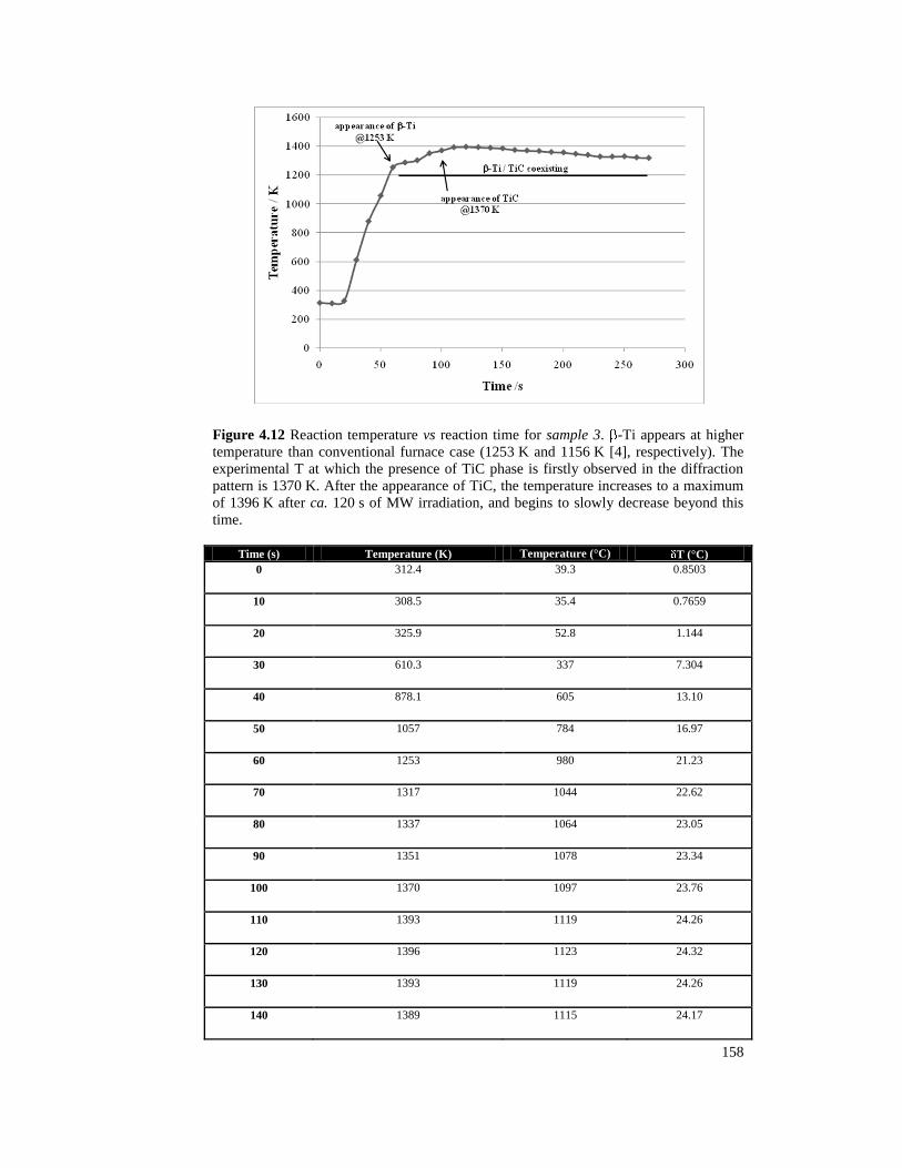
158
Figure 4.12 Reaction temperature vs reaction time for sample 3. -Ti appears at higher
temperature than conventional furnace case (1253 K and 1156 K [4], respectively). The
experimental T at which the presence of TiC phase is firstly observed in the diffraction
pattern is 1370 K. After the appearance of TiC, the temperature increases to a maximum
of 1396 K after ca. 120 s of MW irradiation, and begins to slowly decrease beyond this
time.
Time (s) Temperature (K) Temperature (°C) T (°C)
0 312.4 39.3 0.8503
10 308.5 35.4 0.7659
20 325.9 52.8 1.144
30 610.3 337 7.304
40 878.1 605 13.10
50 1057 784 16.97
60 1253 980 21.23
70 1317 1044 22.62
80 1337 1064 23.05
90 1351 1078 23.34
100 1370 1097 23.76
110 1393 1119 24.26
120 1396 1123 24.32
130 1393 1119 24.26
140 1389 1115 24.17

159
150 1385 1112 24.08
160 1374 1100 23.85
170 1370 1097 23.75
180 1367 1094 23.69
190 1360 1087 23.53
200 1357 1083 23.47
210 1347 1073 23.26
220 1339 1065 23.09
230 1328 1054 22.85
240 1328 1054 22.85
250 1330 1056 22.89
260 1322 1049 22.72
270 1319 1045 22.64
Table 4.3 Data for Fig. 4.12 (where reaction temperature vs reaction time is plotted, for
sample 3).
Figure 4.13 Reaction temperature vs reaction time for sample 4.The phase
transition occurs after ~20 s, at a much lower temperature (648 K) than both sample 3
and conventional furnace. The experimental T at which the presence of TiC phase is
firstly observed in the diffraction pattern is 1322 K. After the appearance of TiC, the
temperature increases up to a maximum of 1603 K (after ca. ~70 s of MW irradiation),
and slowly decreases thereafter.
0
500
1000
1500
2000
0 20 40 60 80 100
Tem
per
atu
re /
K
Time / s
Appearance of -Ti
@648 K Appearance of TiC
(pure phase)
@1322 K

160
Time (s) Temperature (K) Temperature (°C) error on T
0 257 -- 0.355
10 233 -- 0.880
20 648 375 8.13
30 888 615 13.3
40 1080 807 17.5
50 1322 1049 22.7
60 1329 1056 22.9
70 1603 1329 28.8
80 1512 1239 26.8
90 1445 1172 25.4
100 1348 1075 23.3
Table 4.4 Data for Fig. 4.13 (reaction temperature vs reaction time for sample 4).
4.2.2.5 SEM
Although sample 2, 3 and 4 have been all processed in a high power MW
set-up (Gaerling and Sairem® set-up, respectively) and all have been
synthesised starting from dry pellets of -Ti and C graphite in 1:1
stoichiometric ratio, they show differences in SEM pictures.
Sample 2 (1 kW) shows irregular particles with sizes of up to a few
microns (Fig. 4.14 (a)). Sample 3 (500 W) shows spherical crystallites of
10-50 m (Fig. 4.14 (b)). Sample 3 has very different particles shape
compared to sample 2 - possibly due to only partial conversion of the
reactants ( -Ti+C) into TiC.
Sample 3 and sample 4 (Fig. 4.14 (c)) looks similar. The latter also shows
well-formed spheres.

161
(a)
(b)

162
(c)
Figure 4.14 (a) SEM picture (20 m resolution) for sample 2 (SMC, Gaerling set-up, 1
kW, 10 min process); (b) SEM picture (20 m) for sample 3 (Sairem set-up, 0.500 kW);
(c) SEM picture (20 m) for sample 4 (Sairem set-up, 0.500 kW).
Fig. 4.15 shows a SEM picture (20 m) for sample 1 (MMC, 0.800 kW). It
shows irregular particles with sizes of up to a few microns

163
Figure 4.15 SEM images of sample 1 (MMC, 800 W).
4.2.2.6 Raman spectroscopy
Selected samples (sample 1, 3 and 4) were analysed by Raman
spectroscopy, in order to determine if any amorphous phases were present
at the end of the reaction.
Neither stoichiometric TiC nor Ti have Raman-active vibrational modes.
The spectrum of graphitic carbon, instead, contains bands signals at 260,
420, 605, 1320 and 1590 cm-1
; the last two bands are assigned to A1g and
E2g vibrational modes, respectively
[17, 18]. The Raman spectra of
commercially available graphite and TiC (from literature data) are shown
in Fig. 4.18 (a) and (b), respectively. TiC exhibits all the bands of

164
graphite, suggesting that unreacted carbon is present in the TiC powder
[17]. A possible explanation for the low peak intensities in commercially
available TiC is that the bulk of the material may be stoichiometric TiC,
which has no Raman-active vibrational modes.
(a) (b)
Figure 4.16 (a) Raman spectra (literature data) taken from different particles of
commercially available graphite [17]. (b) Raman spectra (literature data) of commercially
available TiC powder (Aldrich, purity of 98%) [17], taken from seven different particles.
Figs. 4.17, 4.18, and 4.19 show Raman spectra for samples 1, 3 and 4,
respectively. In all cases, two broad peaks are visible around 260, 420,
605, 1320 and 1590 cm-1
, which indicates the presence of unreacted
carbon in the sample, attributed to the graphite used as susceptor.
A1g
E2g
A1g E2g

165
Figure 4.17 Raman spectrum for sample 1(MMC, 800 W).
Figure 4.18 Multiplot of Raman spectra for sample 3, collected from different region of
the same sample (SMC, 500 W).
0
500
1000
1500
2000
2500
50 250 450 650 850 1050 1250 1450 1650 1850 2050 2250 2450 2650 2850
Inte
nsi
ty (
a.u
.)
wavenumbers (cm-1)
0
20
40
60
80
100
120
140
160
180
50 250 450 650 850 1050 1250 1450 1650 1850 2050 2250 2450 2650 2850
Inte
nsi
ty (
a.u
).
wavenumber (cm-1)
A1g E2g
A1g E2g

166
Figure 4.19 Multiplot of Raman spectra for sample 4, collected from different regions of
the same sample (SMC, 500 W).
4.3 Discussion and Conclusion
Results from syntheses performed in both MMC and SMC reactors
demonstrated that it is possible to produce TiC, in air, by using -Ti and
graphite as a source of carbon, in a time range of minutes (MMC, sample
1) or even seconds (SMC, sample 3 and 4).
Primarily focusing on sample 3 and sample 4 (in situ SMC reactions),
some considerations can be drawn.
First, in sample 3, the transition phase, (occurring at 1156 K in
conventional furnace [4]) was observed at 1253±21 K in the diffraction
pattern, while in sample 4, it was observed at 648 K (cf. Figs. 4.12 and
4.13 and related Tables 4.2 and 4.3). Nonetheless, in both samples 3 and 4,
0
100
200
300
400
500
600
700
50 250 450 650 850 1050 1250 1450 1650 1850 2050 2250 2450 2650 2850
Inte
nsi
ty (
a.u
.)
wavenumber (cm-1)
A1g E2g

167
the experimental T at which the presence of TiC phase is firstly observed
in the diffraction patterns is similar: 1370±23.7 K and 1322±22.7 K,
respectively (and both higher than the conventional case: T~1073 K [4]),
but the time of formation of TiC is ~100 s in sample 3 and ~50 s in sample
4.
This suggests that, in the case of MW induced formation of Ti-C from Ti
+ C, the transition acts as a trigger mechanism for this reaction, and
the lower the temperature for this transition, the quicker the formation of
TiC. This phase transition occurs at a lower temperature than in the
conventional case, ca. 1200 K [4], and the reaction is several orders of
magnitude faster.
Second, by comparing the temperature at which TiC appears in the
diffraction pattern in sample 4 (1322 K) - with the conventional furnace
case (~1073K [4], Fig. 4.22) the former is higher than the latter by ~300K.
In the MW case, the temperature was calculated by using graphite as an
“internal thermometer”, (thus basically obtaining the bulk temperature),
while in the case of conventional furnace, Winkler et al. registered the
temperature by means of a thermocouple mounted on the sample.
Consequently, the difference between the two cases could be possibly
ascribed also to temperature measurement methods (and related errors).

168
Figure 4.20 Time-temperature plot for the conventional solid state reaction of Ti + C, as
reported by Winkler et al. [4].
Third, in sample 3, -Ti and graphite are the initial reactants, -Ti is
visible after 60 s of reaction (at T = 1253±21.23 K), while TiC peaks
appear after 100 s (T=1370±23.7 K) – compared with 250 min and
T~1073 K in a conventional furnace [4]. Moreover, even if the -Ti
concentration slowly decreases (Fig. 4.21), it is always present in the
reaction mixture, concomitantly with TiC.
In sample 4, -Ti peaks can be detected in 20 s and the temperature
continously increases (Fig. 4.13). The -Ti concentration also increases
(red line, in Fig. 4.22), while -Ti concentration decreases (blue line, in
Fig. 4.24). TiC appears in 50 s, when T=1322±22.7 K (green line, in Fig.
4.22). As stated in Eq. 2.2, Chapter 2, in Section 2.1, the power dissipated
in the material is proportional to the electric field strength inside the

169
Figure 4.21 Phase fraction in sample 3. Although the -Ti concentration slowly
decreases, it never disappears and always coexists with TiC.
material squared, which in turn is a function of the cavity dimensions and
design. In both the sample 3 and 4 cases, the dimensions of the cavity and
the design are exactly the same. However, as the difference between the
two experiments relies in the position of the sample in the cavity, the
higher speed of formation of -Ti phase (and consequently of TiC) in
sample 4 could be ascribed to the creation of higher power density than in
sample 3, thanks to a better position of the sample in the cavity. Although
the P (=FP-RP) on MW generator provided the same result in the cases
(500 W), the difference in MW power absorbed might have been small
and below the sensitivity of the instrument. Consequently, as the position
of the sample in the cavity has been shown to be a crucial initial step in the
0
10
20
30
40
50
60
70
80
90
100
0 50 100 150 200
ph
ase
fra
ctio
n (
%)
time (s)
-Ti (blue)
-Ti (red)
TiC (green)

170
success of the reaction, this aspect requires further investigation and future
studies.
Figure 4.22 Phase fraction vs reaction time for -Ti (blue), -Ti (red) and TiC (green), in
the SMC synthesis of sample 4.
Further, by comparing sample 2 (Gaerling SMC) and sample 3 and 4
(Sairem® SMC), it is interesting to observe that different amount of MW
power (1000 W and 500 W, respectively) and different irradiation times
(ca. 10 min and few seconds, respectively) lead to different particle shape
of the products. Only in sample 3 and 4 spherical particle formation is
observed, while sample 1 and 2 show mostly irregular particle size.

171
4.4 Preliminary Results on Other Binary and Ternary
Systems and Future Studies.
This last part of the thesis is devoted to the process of different chemical
systems in the SMC-MW reactor, by using the same experimental
conditions and the same set-up (Sairem) already used for TiC. Tantalum
(Ta) and tungsten (W) - and their related oxides, Ta2O5 and WO2
respectively - were mixed with Ti and graphite, in different stoichiometric
ratios (see Table 4.5).
As said in Chapter 1, the majority of these compounds are classified as
“cermets”. In particular, in the case of Ti-containing carbide cermets with
Ni, Fe, Mo, Al, Co, Cu, and W, self propagating high temperature
synthesis (SHS), combustion synthesis (CS), and mechanical alloying of
powder mixtures at room temperature are the most common alternatives to
traditional high temperature ceramic synthesis routes [19-24]. The latter
still require a huge instrumentation regarding melting the metal and
graphite under vacuum at a very high temperature.
MW could represent a time-saving, cost-effective and “green” way of
producing such materials. Preliminary results of the fast MW synthesis
probed by means of in situ PND of selected TiC-based cermets is reported
hereafter.

172
4.4.1 Experimental details
The chemical systems listed below were prepared by grinding the
respective elemental or oxide powders in appropriate stoichiometric ratios
in an agate mortar. Each powder sample was cold pressed uniaxially in an
8 mm pellet die (Specac, 5 Tons, 5 min). The pressed pellets were
embedded in the susceptor (graphite) in an open, 10 mm quartz tube. The
Sairem MW set-up used has been extensively described in the previous
Chapters 3.
A list of all the chemical 30 ternary systems processed in situ on D20 - in
the Sairem SMC set-up, at ILL - is reported in Table 4.5.
System
number
Chemical systems and
specification of reactants
Stoichiometric
Ratio
Ti-Ta-C (samples 1-9).
Ta = average particle size −325 mesh,
Aldrich 99.9%
Ti = average particle size -100 mesh
Aldrich 99.7 %
C = average particle size <45 m,
Aldrich 99%
1) Ti – Ta – C (0.1:0.9:2)
2) Ti – Ta – C (0.2:0.8:2)
3) Ti – Ta – C (0.3:0.7:2)
4) Ti – Ta – C (0.4:0.6:2)
5) Ti – Ta – C (0.5:0.5:2)
6) Ti – Ta – C (0.6:0.4:2)
7) Ti – Ta – C (0.7:0.3:2)
8) Ti – Ta – C (0.8:0.2:2)

173
9) Ti – Ta – C (0.9:0.1:2)
Ti-W-C (samples 10-19).
W = average particle size 12 m,
Aldrich 99.9%
Ti = average particle size -100 mesh
Aldrich 99.7 %
C = average particle size <45 m, Aldrich
99%
10) Ti – W – C (1:1:1)
11) Ti – W – C (0.1:0.9:1)
12) Ti – W – C (0.2:0.8:1)
13) Ti – W – C (0.3:0.7:1)
14) Ti – W – C (0.4:0.6:1)
15) Ti – W – C (0.5:0.5:1)
16) Ti – W – C (0.6:0.4:1)
17) Ti – W – C (0.7:0.3:1)
18) Ti – W - C (0.8:0.2:1)
19) Ti - W - C (0.9:0.1:1)
Ti-WO2-C (samples 20-26).
WO2 = average particle size -100
mesh,
Aldrich 99.9%
Ti = average particle size -100 mesh
Aldrich 99.7 %
C = average particle size <45 m, Aldrich
99%
20) Ti –WO2 – C (0.3:0.7:1)
21) Ti –WO2 – C (0.4:0.6:1)
22) Ti –WO2 – C (0.5:0.5:1)
23) Ti –WO2 – C (0.6:0.4:1)
24) Ti –WO2 – C (0.7:0.3:1)
25) Ti –WO2 – C (0.8:0.2:1)

174
26) Ti –WO2 – C (0.9:0.1:1)
Ti-Ta2O5-C (samples 27-30).
Ta2O5 = average particle size <20 m,
Aldrich 99.9%
Ti = average particle size -100 mesh
Aldrich 99.7 %
C = average particle size <45 m, Aldrich
99%
27) Ti –Ta2O5 – C (0.6:0.4:2)
28) Ti –Ta2O5 – C (0.7:0.3:2)
29) Ti –Ta2O5 – C (0.8:0.2:2)
30) Ti –Ta2O5 – C (0.9:0.1:2)
Table 4.5. All the systems processed by means of in situ MWs, in Sairem set-up, at ILL.
Stoichiometric ratios were chosen in order to observe the role (i.e., on the speed and the
nature of product formation) of different concentration of Ti in the mixture.
4.4.2 Preliminary Results and Discussion
4.4.2.1 Ti–Ta–C system.
Diffractograms for all the Ti(1-x)TaxCy compositions are shown in Fig.
4.23. Each pattern was collected on D20 with a 5 min acquisition time,
90° take off angle and wavelength of 1.54 Å. For each stoichiometric
mixture, only the product of the reaction is reported (and not the entire
pathway), in order to easily compare all the systems.

175
Figure 4.23. Diffractograms for Ti(1-x)TaxCy system (x=0.1-0.9, x = 0.1 and y=2). From
the bottom, in black, TaTiC (1:1:2 ratio); in red, Ti0.1Ta0.9C2; in green, Ti0.2Ta0.8C2; in
blue, Ti0.3Ta0.7C2; in yellow, Ti0.4Ta0.6C2 ; in turquoise Ti0.5Ta0.5C2; in pink, Ti0.6Ta0.4C2;
in dark green, Ti0.7Ta0.3C2 ; in orange, Ti0.8Ta0.2C2 ; and in violet Ti0.9Ta0.1C2. For
comparison, MW-processed TiC (in cyan) has been reported (sample 4, as described in
Chapter 4). For clarity, diffractograms have been normalized at 0, 10000, 20000, 30000,
40000, 50000, 60000, 70000, …, 100000 by shifting their intensity and adding a constant
of, respectively, 0, 10000, 20000, 30000, 40000, 50000, 60000, 70000, …, 100000.
By irradiating TiTaC2 pellet by means of MWs (500 W), two new peaks at
ca. 36 ° and 72 ° 2 (Fig. 4.23 (black line)) appear in the diffractogram.
In all the cases, with increasing temperature, a shift of C peaks to lower 2
angles is observed (which return to the original position when the system
cools down, i.e., when the MWs are switched off).
TiC
TiC
C
C C C C
Ta

176
4.4.2.2 Ti-W-C system.
Fig. 4.24 shows the product of the in situ reaction for each stoichiometric
ratio, for Ti-W-C system. For comparison, the cyan diffractogram shows
TiC, as obtained in the same MW reactor (cf. sample 4).
As in Ti-Ta-C system, also for Ti-W-C mixtures, and, in particular, for the
nominal Ti0.5W0.5C, Ti0.6W0.4C, Ti0.7W0.3C, Ti0.8W0.2C, and Ti0.9W0.1C
compounds, characteristic TiC peaks at 31 °2 and 73 °2 are clearly
visible; however, with different reaction times (150, 100, 200, 200, 300
and 150 s, respectively). In all the cases, these peaks are broader than the
reference TiC.
Figure 4.24 Diffractograms for each of the mixture in the Ti(1-x)WxCy system (x=0.1-0.9
x = 0.1 and y=1). Starting from the bottom, in black, TiWC (1:1:1 ratio). Going
upwards, Ti0.1W0.9C1 (in red), Ti0.2W0.8C1 (in green), Ti0.3W0.7C1 (in blue), Ti0.4W0.6C1 (in
maroon), Ti0.5W0.5C1 (in turquoise), Ti0.6W0.4C1 (in pink), Ti0.7W0.3C1 (in dark green),
Ti0.8W0.2C1 (in orange), Ti0.9W0.1C1 (in violet). Cyan line belongs to the MW-processed
TiC (as described in Chapter 4, sample 4).
TiC
TiC
C
C C C C
W

177
4.4.2.3 Ti-WO2-C system
Fig. 4.25 shows the product of MW irradiation in the Ti-WO2-C case.
Again in the Ti-WO2-C case, the characteristic peaks belonging to the
formation of the carbide structure can be observed in samples having a
higher concentration of Ti, namely Ti0.9(WO2)0.1C1, Ti0.8(WO2)0.2C1,
Ti0.7(WO2)0.3C1, Ti0.6(WO2)0.4C1 shifted, in this case, to lower 2 angles of
26 ° and 51 °2 .
Figure 4.25. Ti(1-x)(WO2)xCy with (x=0.3-0.9 x = 0.1) and (y=1). From the bottom,
Ti0.3(WO2)0.7C1 (in blue), Ti0.4(WO2)0.6C1 (in maroon), Ti0.5(WO2)0.5C1 (in turquoise),
Ti0.6(WO2)0.4C1 (in pink), Ti0.7(WO2)0.3C1 (in dark green), Ti0.8(WO2)0.2C1 (in orange),
Ti0.9(WO2)0.1C1 (in violet).
C C
C carb
ide
WO2

178
4.4.2.4 Ti–Ta2O5-C system
More complex than the other systems presented above is the Ti-Ta2O5-C
case, which did not respond to the presence of the MW electromagnetic
field. In the four considered stoichiometric mixtures, in fact, no evidence
of structural changes are visible either the modified TiC-like phases –
formed in the above cases – are formed. This could be due to different
issues which require further investigation, from both an instrumental and a
chemical point of view. For example, it would be interesting repeating the
same mixtures, in order to understand if the position of the sample in the
reactor can be optimised and/or considering other stoichiometric ratios
which could give a better and a faster response to the MW field.
Fig. 4.26 shows the product of reaction for each stoichiometric ratios
studied.

179
Figure 4.26. Diffractograms for Ti(1-x)(Ta2O5)xCy system (x=0.6-0.9 x = 0.1 and y=2).
From the bottom, Ti0.9(Ta2O5)0.1C2 (in pink), Ti0.8(Ta2O5)0.2C2 (in green), Ti0.7(Ta2O5)0.3C2
(in blue), Ti0.6(Ta2O5)0.4C1 (in yellow), Ti0.5(Ta2O5)0.5C2 (in turquoise), Ti0.4(Ta2O5)0.6C2
(in pink), and Ti0.3(Ta2O5)0.7C2 (in dark green).
4.4.3 Discussion and Conclusion
For all the systems described, except in the case of Ta2O5-TiC, it is
observed that a higher concentration of Ti in the mixture lead to the TiC
formation in a time range relatively low (around 2-3 minutes, on average).
When the content of Ti in the mixture is decreased, no response to the
MW field is observed.
This could be possible due to the fact that the metal – or also the oxide –
addition in the TiC-based mixture mainly played a role of a catalyst for the
reaction, thus making possible the TiC formation [20].
C
C C
Ta2O5

180
However, further physical-chemical investigations and characterisations of
all the systems are required, in order to understand:
1) if the MW set-up plays a role in the systems formation and it is,
therefore, possible to implement the instrumentation for processing
systems prepared with a low content of Ti.
2) if these compounds could be classified as new cermets in terms of their
observed properties;
3) if it is possible to implement the methodology for the Ta2O5-TiC
system.
References
1. Lee, D.W., S. Alexandrovskii, and B.K. Kim, Mg-thermal
reduction of TiCl4+CxCl4 solution for producing ultrafine titanium
carbide. Materials Chemistry and Physics, 2004. 88(1): p. 23-26.
2. Zhang, H., et al., Preparation of titanium carbide powders by sol-
gel and microwave carbothermal reduction methods at low
temperatures. . Journal of Sol-Gel Science and Technology, 2008.
46: p. 217-222.
3. Mohapatra, S., D.K. Mishra, and S.K. Singh, Microscopic and
Spectroscopic Analysis of TiC Powder Synthesized by Thermal
Plasma Technique. Powder Technology, 2013. 237: p. 41-45.
4. Winkler, B., et al., In situ observation in the formation of TiC from
the elements by neutron diffraction. Journal of Alloys and
Compounds, 2007. 441: p. 374-380.
5. Ahmad, I., R. Dalton, and D. Clark, Unique Application of
Microwave Energy to the Processing of Ceramic Materials.
Journal of Microwave Power and Electromagnetic Energy, 1991.
26(3): p. 128-138.
6. Hassine, N.A., J.G.P. Binner, and T.E. Cross, Synthesis of
Refractory Metal Carbide Powders via Microwave Carbothermal
Reduction. International Journal of Refractory Metals & Hard
Material, 1995. 13: p. 353-358.

181
7. Menéndez, J.A., et al., Microwave heating processes involving
carbon materials. Fuel Processing Technology, 2010. 91: p. 1-8.
8. Rao, K.J., et al., Synthesis of Inorganic Solids Using Microwaves.
Chemical Materials, 1999. 11: p. 882-895.
9. Ohlsson, T. and P.O. Risman, Temperature distribution of
microwave heating - spheres and cylinders. Journal of Microwave
Power and Electromagnetic Energy, 1978. 13(4): p. 303-309.
10. Wood, R.M., The lattice constants of high purity alpha titanium.
Proceedings of the Physical Society, 1962. 80: p. 783-786.
11. Hull, A.W., Structure of graphite. Physical Review, 1917. 10: p.
661-696.
12. Burgers, W.G. and F.M. Jacobs, Crystal structure of beta-titanium.
Zeitschrift für Kristallographie, Kristallgeometrie, Kristallphysik,
Kristallchemie, 1936. 94: p. 299-300.
13. Becker, K. and F. Ebert, Die Kristallstruktur einiger binarer
Carbide und Nitride. Zeitschrift für Physik A Hadrons and Nuclei,
1925. 31(1): p. 268-272.
14. Wang, J., et al., Evidence for the Microwave Effect During Hybrid
Sintering. Journal of the American Ceramic Society, 2006. 89(6):
p. 1977-1984.
15. Harrison, A., et al., In situ neutron diffraction studies of single
crystals and powders during microwave irradiation. Faraday
discussions, 2002. 122: p. 363-379.
16. Nihira, T. and T. Iwata, Temperature Dependance of Lattice
Vibrations and Analysis of the Specific Heat of Graphite. Physical
Review B, 2003. 68: p. 134305-16.
17. Lohse, B.H., A. Calka, and D. Wexler, Raman spectroscopy as a
tool to study TiC formation during controlled ball milling. Journal
of Applied Physics, 2005. 97: p. 114912-7.
18. Klein, M.V., J.A. Holy, and W.S. Williams, Raman scattering
induced by carbon vacancies in TiCx. Physical Review B, 1978.
17(4): p. 1546-1556.
19. Choi, Y., J.K. Lee, and M.E. Mullins, Densification process of
TiCx–Ni composites formed by self-propagating high-temperature
synthesis reaction. Journal of Materials Science, 1997. 32(7): p.
1717-1724.
20. Fan, Q., H. Chai, and Z. Jin, Role of iron addition in the
combustion synthesis of TiC–Fe cermet. Journal of Materials
Science, 1997. 32(16): p. 4319-4323.
21. Dunmead, S.D., et al., Kinetics of Combustion Synthesis in the Ti-
C and Ti-C-Ni Systems. Journal of the American Ceramic Society,
1989. 72(12): p. 2318-2324.
22. LaSalvia, J.C. and M.A. Meyers, Combustion synthesis in the Ti-
C-Ni-Mo system: Part II. Analysis. Metallurgical and Materials
Transactions A, 1995. 26(11): p. 3011-3019.

182
23. Brinkman, H.J., et al., Production of Al–Ti–C grain refiner alloys
by reactive synthesis of elemental powders: Part I. Reactive
synthesis and characterization of alloys. Journal of Materials
Research, 2000. 15(12): p. 2620-2627.
24. Bandyopadhyay, S., H. Dutta, and S.K. Pradhan, XRD and
HRTEM characterization of mechanosynthesized Ti0.9W0.1C
cermet. Journal of Alloys and Compounds, 2013. 581(0): p. 710-
716.

183
Chapter 5
Conclusions and Future Studies.
The work described in this thesis focuses on the MW synthesis of a
ceramic material, TiC. In particular, the development of a general
experimental procedure to afford the desired material and the study of its
reaction pathway by means of in situ neutron diffraction are the major
goals achieved. It has been demonstrated, in fact, that it is possible to
produce TiC – traditionally synthesised via time demanding processes (24-
48h) and high temperatures (1900-2300 K) – in second timescale, in a
single mode MW reactor.
The final experimental procedure consisted of a 10 mm quartz tube (sealed
at one end), containing the sample pellet (8 mm diameter, 1 g, 1 cm
thickness) imbedded in graphite powder (acting as a susceptor), in the
single mode cavity. The susceptor was required after initial investigation
revealed no heating of the metal and carbon reaction mixture. Graphite,
capable of absorbing the MW radiation and raising the reaction
temperature, was used to help initiate carbide formation. However, careful
use of the susceptor was required; too much would not allow sufficient
MW energy to penetrate to the sample and too little would not provide
adequate heat to raise the initial reaction temperature. The reaction was
performed at ambient pressure.

184
The applied microwave power and the design of the set-up were also very
important parameters which lead to the success of the reaction.
In the case of the Sairem cavity (described in Chapter 3) different
geometries were tested prior the final (and working) configuration.
This single mode MW system is now available for users and fully
operational on D20, at ILL. Further, it has been designed in such a way
that it can easily fit the D20 beam line vessels, thus making possible
reactions under vacuum, if needed.
TiC was also successfully obtained in a DMO, in 10 minutes, in air.
However, as DMOs do not permit the control on several parameters
(tuning of MW power, position of the sample in the cavity, possibility of
in situ reactions), single mode MW cavity remains the best choice, despite
of its higher costs and design difficulties.
It has been also demonstrated that this SMC-MW reactor is capable of
processing different systems of higher complexity, such as ternary
titanium-containing carbides (TixTa(1-x)C, TixW(1-x)C, Tix(WO2)(1-x)C, and
Tix(Ta2O5)(1-x)C). Preliminary results demonstrated that a higher amount of
Ti in the mixture can lead to the formation of TiC in a relatively short time
(2-3 minutes).
In conclusion, much of the work published in this thesis adds knowledge
to MW apparatus design for solid state materials processes.
The contributions can be defined as follows:

185
- The development of a reproducible process for the successful MW
synthesis of transition metal carbides in unprecedented timescales.
- Design and optimisation of a MW set-up capable of performing in situ
reactions, thus giving insight in fast MW reactions, for the first time.
Future work could be focused on how incident power, reactor design,
position of the sample in the cavity, and/or use of water as binder17
can
influence the process. Further, it would interesting to understand how
these parameters might enhance the physical-chemical properties of
products.
17 In a precedent PhD project, it has been seen that an important factor in MW-promoted
reactions is the use of water as binder – used in the pellet making process – which is
believed to minimise the intergrain void space between particles and to act as a polar
liquid MW susceptor (Carassiti L., Synthesis of silicon carbide ceramics by novel
microwave methods, PhD thesis, University of Glasgow, 2011).