new computational method in engineering
DESCRIPTION
Modeliranje na racunaruTRANSCRIPT


NEW COMPUTATIONAL CONCEPTS IN CIVIL ENGINEERING
Rodian Scînteie, Costel Pleşcan - editors -
Editura Societăţii Academice “Matei - Teiu Botez” Iaşi 2010

Proceedings of the 8th International Symposium
Computational Civil Engineering 2010 Descrierea CIP a Bibliotecii Naţionale a României
New computational concepts in civil engineering / ed.: Rodian Scînteie, Costel Pleşcan. - Iaşi : Editura Societăţii Academice "Matei - Teiu", 2010 Bibliogr. ISBN 978-973-8955-87-5
I. Scînteie, Rodian (ed.) II. Pleşcan, Costel (ed.)
624
Editura Societăţii Academice "Matei - Teiu Botez" B-dul Dumitru Mangeron nr. 43 Director: Prof.univ.dr.ing. Constantin Ionescu, e-mail:[email protected]
All rights reserved, © Societatea Academică “Matei - Teiu Botez”, Iaşi, România, 2010

“Computational Civil Engineering 2010”, International Symposium Iasi, Romania, May 28, 2010
Table of Contents
1. Adrian-Mircea Ioani, Hortensiu-Liviu Cucu Resistance to progressive collapse of RC structures: principles, methods and designed models 5
2. Adrian-Mircea Ioani, Hortensiu-Liviu Cucu Improving resistance to progressive collapse of concrete structures through seismic design (P100-92, P100-1/2006) 19
3. Ioana LADAR, O. PRODAN, P. ALEXA A new approach to assessment of seismic mitigation via passive protection 35
4. Alexandra-Denisa Danciu, Eugen Pantel, Horatiu-Alin Mociran, Dan –Ioan Danciu Resistance to progressive collapse of RC structures: principles, methods and designed models 47
5. Alexandru Cătărig, Ludovic Kopenetz Ecostructures 53
6. Amir Hossein Alavi, Amir Hossein Gandomi, Ali Mollahasani, Azadeh Rashed Nonlinear Modeling of Soil Cohesion Intercept Using Generalized Regression Neural Network 69
7. Sergiu Andrei Băetu, Ioan Petru Ciongradi, Georgeta Văsieș Static nonlinear analysis of structural reinforced concrete walls energy dissipators with shear connections 87
8. Cătălin Banu, Nicolae Ţăranu, Gabriel Oprişan, Vlad Munteanu Finite Element Analysis of Fiber Reinforced Polymers Bars 99
9. J.A. Valcárcel, L. G. Pujades, A. H. Barbat, M.G Mora and O.D Cardona Formulation of an integrated Hospital Risk Index 106
10. Y.F. Vargas, L.B. Pujades, A. H. Barbat, J.E. Hurtado Probabilistic evaluation of the seismic damage of reinforced concrete structures 122
11. Jiri Brozovsky, David Prochazka, Dalibor Benes Paving Blocks Compressive Strength Evaluation by Impact Hammer 138
12. Jiri Brozovsky, David Prochazka Concrete durability with addition of fluidized ash in sulphate and chloride aggressive environment 146
13. Sergiu Călin, Mugurel Cloşcă, Gabriela Dascălu, Ciprian Asăvoaie Computational simulation for concrete slab with spherical gaps 154
14. Vít Černý, Rostislav Drochytka, Karel Kulísek Environmental impact analysis of artificial aggregate burning process 162
15. Ciprian Cozmanciuc, Ruxandra Oltean, Nicolae Taranu Analytical models for confinement systems of reinforced concrete columns with circular and noncircular cross sections utilizing composite materials 170
16. Elena Diaconu, Ştefan Marian Lazăr Protection of pavement systems to prevent and combat the phenomenon of freezing-thaw 183

2 Table of Contents
17. Geanina Cosmina ADAM1, Gabriel Iulian MIHAI Developing the computational urban systems in Romania based on the survey data 192
18. Geanina Cosmina ADAM, Gabriel Iulian MIHAI, Anca Alina LAZĂR Modern specific software used in structural engineering, architecture, urbanism and town planning 199
19. Sunai Gelmambet, Florin Ţepeş Studies and research on the calculation of the shear stress for light-gauge steel profiles at bending 205
20. I. Radinschi, C. Damoc, B. Aignatoaie, V. Cehan Improving the e-Learning of Engineering Physics with the Aid of Adobe Flash 219
21. Mihail Iancovici, Bogdan Ștefãnescu Standard vs. time-domain approach for seismic performance analysis of tall buildings 227
22. Ioana Olteanu, Mihaela Anechitei, Ionut-Ovidiu Toma, Mihai Budescu Numerical Investigation on Plastic Hinge Development in Reinforced Concrete Structures Using Pushover Analysis 240
23. Irene Daprà, Giambattista Scarpi Numerical solution for unsteady plane flow of dilatant fluids 248
24. Ferencz Lazar-Mand, Dragoş Florin Lişman Practical aspects concerning nonlinear dynamic analysis 257
25. Ludovic Kopenetz, Alexandru Cătărig Structural analysis problems of complex structures 271
26. Tomáš Melichar Analysis for the use of fire sand as alternative filler in the manufacture of facing tilling elements based on glass 289
27. Tomáš Melichar, David Procházka, Jiří Bydžovský Ultrasonic impulse method in parameters investigation of glass board composites 301
28. Oana Stanila, George Taranu, Razvan Sencu, Alexandru Stanila, Magda Brosteanu Necessary emergency shelters after natural disasters 310
29. Oana Mihaela Ioniţă, Nicolae Ţăranu, Mihai Budescu An efficient way of improving the safety of reinforced concrete frame structures against impact loading 329
30. Paul Mutică, Silivan Moldovan, Ioana Moldovan Advanced 3D Modeling in ArchiCAD. Basic GDL scripting 346
31. David Procházka, Jiří Brožovský, Vít Černý Shielding Mortar Design for Protection of Rooms Exposed to X-Ray 358
32. David Procházka, Klára Křížová, Tomáš Melichar High Strength Concrete Design Problematics 364
33. Elena Puslau, Costel Plescan Specific Pavement Condition Indicators for rigid and flexible pavements 370

“Computational Civil Engineering 2010”, International Symposium 3
34. Carmen Răcănel, Adrian Burlacu Time behavior changing of a pavement structure depending on asphalt layer characteristics 382
35. Ruxandra Oltean, Ciprian Cozmanciuc, Nicolae Taranu Analytical models for bond behavior between FRP strips and concrete 395
36. Paul Mutică, Silivan Moldovan, Ioana Moldovan CAD Software as a Tool in Design 406
37. Salim Sadi Studies on Reinforced Concrete Constitutive Laws and Development of a Related Computer Program 412
38. Stanciu A, Iliesi A. T., Lungu I. Comparative analysis regarding settlement prediction founded on collapsible soils 429
39. Ţepeș Onea Florin, Gelmambet Sunai Comparative analysis of structural response to various methods of calculation for reinforced concrete frame structures 439
40. Cristina-Alexandra Topală, Valeriu Bănuţ Study of steel frames stability in the elasto-plastic domain 446
41. Vasile-Mircea Venghiac, Ioan Petru Ciongradi, Mihai Budescu Steel structures with composite floors and energy dissipative columns 459
42. Dumitru Moldovan, Cornelia Măgureanu Static Modulus of Elasticity of High Strength Concrete 467
43. Horaţiu-Alin Mociran, Eugen Panţel, Alexandra-Denisa Danciu Application of fluid viscous dampers in the seismic control of steel frame structures 480
44. Gheorghe Ionică Altiscad Intellishape® Software for seismic design of reinforced concrete structures 488

4 Table of Contents
“Computational Civil Engineering 2010”, International Symposium Iasi, Romania, May 28, 2010
Resistance to progressive collapse of RC structures: principles, methods and designed models
Adrian-Mircea Ioani1, Hortensiu-Liviu Cucu1 1Department of Structural Mechanics, Technical University, Cluj-Napoca, 400114, Romania
Summary
Following the U.S. GSA Guidelines (2003), the paper examines the vulnerability to progressive collapse of an existing 13-storey RC framed structure, designed according to the provisions of the Romanian Design Code P100-92 for Bucharest, Romania, a zone of high seismic risk where ks=PGA/g=0.20,Tc=1.5 and βr= 2.5 (Model P100-92).
A similar analysis is made considering that the structure is designed according to the provisions of the last seismic design code P1001/-2006, where the values of some design parameters have been changed: ag=0.24g, Tc=1.6s, β0=2.75 and q=5*1.35=6.7(model P100-2006).
The analyzed structure consists of five 6.0 m bays in the longitudinal direction and two 6.0 m bays in the transverse direction and was seismically designed and detailed at the Ultimate Limit State for the following combination of loads: D+0.4L+E, where D=2.0 kPa + self-weight, L=2.4 kPa. The earthquake E is acting through the total equivalent seismic force given by the Code P100-92 (S=0.0945G) or by the Code P100-1/2006 (S=0.09973G).The magnitude and distribution of potential areas of inelastic demands in the structure are assessed using the concept of DCR (Demand-Capacity-Ratios).
Based on this concept, structural elements that have DCR values exceeding the allowable magnitude (2.0 for typical configuration buildings) are considered to be severely damaged or collapsed. Dynamic properties and internal forces for the analyzed models are determined with the 3-D linear elastic model, created and analyzed in the FEA program AUTODESK ROBOT Structural Analyses Professional 2010.
Taking into account the small changes in the level of equivalent seismic force for the model P100-2006, as well as the authors previous results regarding the elastic behavior in the missing column design situation of the model P100-92, the GSA procedure indicates that medium- rise buildings having RC frames, seismically designed for Bucharest according to P100-1/2006, are not subjected to progressive collapse risk.
KEYWORDS: progressive collapse, load redistribution, RC frames, GSA Guidelines (2003), seismic design.

6 A. Ioani, H. Cucu
1. INTRODUCTION
Abnormal loads such as explosions, vehicle collision, foundation failure are not considered in an ordinary structural design (Su et al. 2009 [1]). But such low-probability events represent the main causes leading to a structural progressive collapse of buildings. Progressive collapse is defined as the spread of an initial local failure from element to element (chain reaction) that leads to partial or even full collapse of an entire structure. In a more general sense, the initial collapse of the local damage can be man-made (explosions, impact by vehicles, human errors, etc.) or natural (wind gusts, floods, earthquakes).
The disastrous consequences of a progressive collapse have been seen since the partial collapse of the Roman Point apartment building in London (1968) [2]) or in the collapse of nearly half of the nine story building-the Alfred P. Murrah Federal Building in Oklahoma City (1995) [3] - when, as a consequence of a terrorist attack, the blast effect abruptly removed an external column (Figure 1).
Progressive collapse has to be an important issue because, as recent terrorist attacks demonstrated, most causalities are due to building collapse rather than the initial explosion or impact (Sasani et al. 2007 [4]).
Figure 1. Failure boundaries in the Roman Point apartment building [2] and in the A.P Murrah Federal Building [3]

“Computational Civil Engineering 2010”, International Symposium 7
The design philosophy of structures subjected to abnormal loads - as they are defined in GSA Guidelines (2003) [5] - Section 2 (“other than conventional design loads dead, live, wind, seismic”) - is to prevent or mitigate damage, not necessarily to avoid the collapse initiation from specific cause. This approach is similar to the concept adopted in any modern earthquake-resistant design codes.
Whereas resistance to progressive collapse is primarily an issue of gravity load-carrying capacity, the design of elements (beams, columns) also depends on demands from other actions such as wind or seismic actions. It means that, if beams, columns or joints of a framed structure had a larger load-bearing capacity due to more sever seismic actions considered in design, these elements would have a higher capacity to confine the damage to the initially affected zone, and consequently to prevent progressive collapse (Sasani et al. 2008 [6]).
Baldridge and Humay (2003) have shown that a 12-story framed structure, seismically designed for a moderate (Zone 2B) or a high seismic zone (Zone 4), does not experience progressive collapse when it is subjected to the “sudden removal” of an exterior column [7].
Bilow and Kamara (2004) [8], analyzing three moment-resisting frame buildings of 12 stories high and each with different seismic design categories (A, C and D), showed that building columns do not require additional reinforcement to prevent progressive collapse. Beams proportioned and detailed according to the seismic category D, have sufficient strength and ductility to resist progressive collapse.
Following the GSA Guidelines (2003) [5], in a previous paper, the authors have examined the vulnerability of a medium-rise building (13-storeys) having a RC framed structure, seismically designed according to the former seismic design code P100-92 [9], for Bucharest (zone C, seismic coefficient PGA/g=0.20). Bucharest was chosen because it is considered as “the city with the highest seismic risk in Romania” and also “the most vulnerable capital of Europe” (Dubina and Lungu 2003 [10]).
The study demonstrated that seismically designed (P100-92 [9]) and detailed (STAS 10107/0-90 [11]) RC moment – resisting frames provide buildings with continuity, redundancy and ductility, and consequently such structures do not experience progressive collapse when subjected to different “missing column” scenarios, according the GSA (2003) criteria (Ioani, Cucu and Mircea 2007 [12]).
2. RESEARCH SIGNIFICANCE
But recent studies (Cretu and Demetriu 2006 [13], Pop and Madularu 2008 [14]) reported – in comparative analyses– that the use in design of the new Romanian seismic design code P100-1/2006 [15] would lead for RC frame structures

8 A. Ioani, H. Cucu (ductility class H), to significant reductions (-17% to -23%) in the magnitude of the global seismic coefficient (c). In the same time, other analyses (Postelnicu and Pascu 2006 [16]) revealed that, for ductile RC structures “practically, the values of seismic forces do not increase” when the design is made following the previsions of the new code P100-1/2006 [15].
On the other hand, nowadays, design of concrete structures should be made according to Eurocode 2 (SR EN 1992-1-1:2004 [17]) and consequently, changes in the type and amount of reinforcement in beams and columns, as well as the new additional rules for longitudinal and transverse reinforcement are expected to produce effects in member’s capacity.
Taking into consideration such aspects, this comparative study investigates the effects on the resistance to progressive collapse of a reinforced concrete frame structure, when the design is made according to the provisions of the present codes P100-1/2006 [15] and SR EN 1992-1-1:2004 [17]. Two models seismically designed according to P100-92 and P100-1/2006 seismic codes, are prepared for analyses to progressive collapse.
3. PRINCIPLES AND DESIGN CODES
To mitigate the risk of progressive collapse, a structure must accommodate the initial local damage and then to develop an alternative load-path to sustain the redistributed loads (Su et al. 2007 [1]). To provide alternative load transfer paths fallowing the loss of an individual member or a load failure, the structure must have an adequate level of continuity, redundancy and ductility; these requirements are found in seismic design as well (Ioani, Cucu and Mircea 2007 [12], Bilow and Kamara 2004 [8]).
Two American federal guidelines GSA (2003) [5] and DOD (2005) [18] adopted this principle and proposed procedures to assess the potential of progressive collapse of a building following the rational removal of certain major load-bearing elements.
The GSA Guidelines [5] are based on the Alternative Path Method (APM) and consider the instantaneous loss of portions of the structure using different “missing column” or “missing beam” scenarios (Figure 2).
Such checks are required, though the cause is not always specified (natural hazard or man-made hazard) in currently used design codes for reinforced concrete structures.
Thus, the Eurocode: Basis of structural design (EN 1990 - Sect. 2.1 (4) P) [19] requires that “structure shall be designed in such way that it will not be damaged

“Computational Civil Engineering 2010”, International Symposium 9
by events like fire, explosions, impact or consequences of human errors, to an extent disproportionate to the original cause”. In addition, Sect. 2.1 (5) P shows that “Potential damage shall be avoided or limited by appropriate choice of one or more of the following: ... selecting a structural form and design, that can survive adequately the accidental removal of an individual member or a limited part of the structure …”.
A description of design standards or guidelines where design rules against progressive collapse are specified is presented in NISTIR 7396/2007 [2]: British Standards, Eurocode, National Building Code of Canada, Swedish Design Regulations, ASCE 7, ACI 318, New York City Building Code, Department of Defense-Unified Facilities Criteria (DOD), General Services Administration (GSA), Interagency Security Committee.
The most recent Romanian seismic design Code P100-1/2006 - Sect. 4.4.1.2 [15] explicitly demands that “seismic design should provide the building structure with an adequate redundancy. In this manner it is ensured that the failure of one single element or the failure of a structural link does not expose the structure to the loss of stability”.
Taking these approaches into account, it seems natural for structural engineers to use their creativity to make structures more resilient to both natural hazard (e.g. earthquakes) and mean-made hazards (e.g. explosions, impact by vehicles) and consequently, the designed structural system will satisfy at the same time, the requirements of lateral-load resistance and those of the prevention of progressive collapse.
Figure 2. Possible blast behavior of frame structure [12]

10 A. Ioani, H. Cucu
4. ASSESSEMENT OF THE POTENTIAL TO PROGRESSIVE COLLAPSE (GSA GUIDELINES 2003)
Progressive collapse is a dynamic and nonlinear event as it takes place in a very short time frame and structural members undergo nonlinear deformations before failure [20]. To analyze rigorously progressive collapse of a structure, nonlinear dynamic analysis should be performed to take account for energy dissipation, large inelastic deformation, materials yielding, crashing and fracture [20].
Nonlinear dynamic analyses require step-by-step integration which are very time consuming, and due to the general lack of structure behavior data especially related to the beam-column connections is difficult to evaluate the results of the analyses. Consequently, nonlinear dynamic analyses is not used in the current design of low and mid-rise building while account for about 93% of buildings in U. S. [20] and for nearly 98% of buildings in Bucharest, Romania [10].
For buildings of 10 storeys or less in height with relatively simple layouts, GSA Guidelines (2003) [5] recommend the alternate load path method (APM) based on a linear elastic analysis, to assess the vulnerability of a new and existing buildings to progressive collapse. Normally used for buildings 10 storeys above grade and less, the method [5] can be successfully applied to taller buildings [7], [8], [12].
To determine the potential of progressive collapse of a typical RC structure, designers can perform a structure linear elastic analysis, considering the instantaneous loss of one of the first floor columns (“missing column” scenarios), as follows (Figure 3):
- an exterior column near to the middle of the short side (case C1 in our study);
- an exterior column near to the middle of the long side (case C2);
- a column located at the corner of the building (case C3);
- a column interior to the perimeter column live fore facilities that have underground parking and/or uncontrolled public ground flow areas (case C4).
Figure 3. Missing column scenarios according to GSA Guidelines (2003) [5]

“Computational Civil Engineering 2010”, International Symposium 11
The sudden loss of a load bearing element (column in this analysis) generates in the “damaged” structure dynamic actions (moments, shear and axial forces) and the structural response is a nonlinear. But, as in the routine seismic design, one simple approach is to use an equivalent linear elastic procedure, considering that the increased vertical forces to be applied to the structure are:
staticLoadLLDLLoad 225.02 (1)
where DL is the dead load and LL is the live load.
In the GSA criteria, live load is reduced since the probability of that the entire full load being present during the event is small. In the same time, by multiplying the static load combination by a factor of 2.0, the method takes into account the dynamic amplification effect due to the instantaneously removed of a vertical support (column).
With this increased gravity forces ( ), demands ( ) in structural
elements and connections are determined in terms of bending moments, axial forces and shear forces. Following the linear static analysis, a Demand-Capacity Ratio (DCR) is computed for each structural element:
staticLoad2 UDQ
CE
UD
Q
QDCR (2)
where is the expected ultimate, un-factored capacity (bending moment, axial
forces, shear forces) of the structural component. CEQ
In the assessment of , strength increase factors are applied to the properties of
the construction materials to account for strain rate effect and material over-strength [7]. For reinforced concrete structures, a material increase factor of 1.25 is allowed for concrete and reinforcing steel [5].
CEQ
In order to prevent collapse of the alternate path structure, the DCR values for each structural element must be less than or equal, to the following [5]:
0.2DCR for typical structural configurations;
5.1DCR for atypical structural configurations.
Using the DCR criteria, structural members and connections that have DCR values greater then 2.0 are considered to be severely damaged or collapsed. If all the computed DCR values are less than or equal to 1.0, then the component is expected to respond elastically to the adopted missing column scenario. In routine design, an element with DCR greater than 1.0 has exceeded its ultimate capacity [7].
For continuous element, Baldridge and Humay (2003) [7] showed that the flexural DCR value at an element section may exceed 1.0, because in this case flexural

12 A. Ioani, H. Cucu demand is redistributed along the length of the elements that have reserve flexural capacity. In the same time, Baldridge and Humay (2003) and also Lew [20] underline that in the case of shear, failure is imminent when DCR value exceeds 1.0; this limit for shear (DCR=1.0) is not considered by Bilow and Kamara (2004) [8] in the assessment of progressive collapse of a RC framed structure (“… all the DCR’s values for shear are below the GSA limit 2.0 and therefore additional shear reinforcement is not needed to prevent progressive collapse”).
5. SEISMICALLY DESIGNED MODELS
5.1. Model P100-92
In order to determine the inherent reserve capacity to progressive collapse of a RC structure erected in a high seismic zone of Romania, the investigation was conducted on a 13-storey RC frame building designed according to the older requirements of the Romanian seismic design code P100–92 [9].
The structure consists of five 6.0 m bays in the longitudinal direction and two 6.0 m bays in the transverse direction and has a story height of 2.75 m, except the first two floors that are 3.60 m high. In the design at the Ultimate Limit State, the Special Combination of loads according to the Romanian Standard STAS 10107/0A-77 [12] is:
D+0.4L+S+E, (3)
representing a combination of dead load D (self-weight and a supplementary dead load of 2 kPa), live load L=2.4 kPa with a load long term factor of 0.4, and the earthquake effect (E).
The seismic analysis is performed for Bucharest (zone C on the Romanian seismic map with ks=PGA/g=0.2). For Romania, the seismic coefficient ks, varies from 0.08 to a maximum value of 0.32 [9]. The magnitude of total equivalent seismic force S that enters the load combination (Equation 3) is calculated as follows (P100-92 [9]):
GGTkS s 0945.0 (4)
G = 49358 kN
The structural response of the model under the Special Combination of loads, and the behavior of the damaged structure (case C1, C2, C3 and C4 of the “missing column” scenarios) is determined with the 3-D linear elastic model, created and analyzed in the FEA program AUTODESK ROBOT [21].

“Computational Civil Engineering 2010”, International Symposium 13
Figure 4. AUTODESK ROBOT Structural Analyses Professional 2010 [21] model of a 13-
storey RC building: missing column scenarios
The model generated by this computer program is shown in Figure 4 and certain details and design data regarding the model are given in Table 1. The material properties are given in Table 2. In the seismic design of the model, design values for strengths have been used. Reinforcement is made following the provisions of the former standard for RC structures STAS 10107/0-90 [11].
Table 1. Design details of structural elements for the model P100-92 Column* Longitudinal
beams* Transverse beams* Storey
Dimens. [mm]
Dimens. [mm]
Dimens. [mm]
Top** longitudinal
steel
Bottom** longitudinal
steel
Stirrups at ends***
1, 2 700x900 350x650 350x700 5Ø25 (1.05%)
4 Ø 25 (0.84%)
Ø 8/140mm (0.207%)
3,4,5 700x750 350x650 350x700 5 Ø 25 (1.05%)
4 Ø 25 (0.84%)
Ø 8/140mm (0.207%)
6,7, 8,9
600x750 300x650 300x700 4 Ø 25 (0.99%)
2 Ø 20+2 Ø 25 (0.81%)
Ø 8/170mm (0.2%)
10,11, 12,13
600x600 300x550 300x600 4 Ø 20 (0.74%)
3 Ø 20 (0.56%)
Ø 8/150mm (0.22%)
*Concrete: Strength class of concrete according to [11] **Reinforcing steel: PC52 type; Ø = bar diameter in mm; (ρl) = reinforcement ratio for longitudinal reinforcement ***OB37 - type for stirrups; (ρw) = reinforcement ratio for shear reinforcement

14 A. Ioani, H. Cucu In the progressive collapse analysis according to the GSA Guidelines provisions, the expected ultimate, un-factored, capacity of the structural elements was determined using the characteristic (un-factored) values for the strengths, multiplied by the strength increase factor of 1.25 ( Table 2).
Table 2. Strengths of materials for the model P100-92 (MPa) Seismic design
Progressive collapse analysis Material
Design values* Characteristic un-factored values
With 1.25 factor
Rc=12.5 Rck=16.6 20.75 Concrete Bc20 Rt=0.95 Rtk=1.43 1.78 Ra=300 Rak=345 431 Steel PC52
OB37 Ra=210 Rak=255 318
* Rc (Rt) = design value of the compressive (tensile) strength of concrete; Ra = design value of the yield strength of reinforcement
5.2. Model P100-1/2006
A similar investigation was conducted considering the same structure, seismically designed according to the provisions of the present seismic code P100-1/2006 [15] and detailed according to Eurocode 2 (SR EN 1992-1-1:2004) [17] – standard which replaced the old national standard for RC structures STAS 10107/0-90 [11]. In the design, the same combination of loads given by Eq (3) is used, were the snow has a new value of S=1.28 kN/m2 for Bucharest.
Consequently, a small change appears in the magnitude of the weight of the structure G=49370 kN.
In the new code P100-1/2006 [15] when the Equivalent Static Seismic Force Method is applied, the seismic base shear force Fb is:
GmTSF dIb 09973.0)( 1 (4)
where:
2.1I , for building of importance class II;
=ordinate of the design spectrum)( 1TSd
q
TaS gd
)(;
1T = fundamental period of vibration of the building for lateral motion, in the
direction considered [15]; s) 1.1337.450.075HC(T 3/43/411
m= total mass of the building above the foundation

“Computational Civil Engineering 2010”, International Symposium 15
= correction factor which takes into account the contribution of the fundamental mode, by its effective modal was ( 85.0 if T1<TC) and the building has more then two story.
The new Romanian seismic map [15] considers that the ground of Bucharest it characterized by
, gag 24.0 sTB 16.0 , sTC 6.1 and 75.2)( 0 T (5)
and consequently :
mq
gF Pb 85.0
75.224.02.12006100 (6)
The code [15] specifies that earthquake resistant structures shall be designed to provide energy dissipation capacity and an overall ductile behavior. Structures located in seismic zones with ag>0.16g (for Bucharest, ag = 0.24g) should be designed according to the requirements of the ductility class H (DCH=high ductility) and the corresponding behavior factor q, for frame systems (Table 5.1 [15]), is:
75.635.10.50.51
uq (7)
where 35.11
u for multi-storey, multi-bay frames.
With q=6.75, the base shear force becomes:
GGmq
aF g
IP
b 09973.085.075.6
175.224.02.102006100
(8)
For the analyzed structure, an increase of 5.5% in the magnitude of the base shear face is reported when the provisions of P100-2006 is applied in the seismic analysis (Fb
P100-2006/ FbP100-92=1.055).
As in the case of model P100-92 the structure response is determined – via the modal analyses – with the 3-D linear elastic model, created and analyzed in the FEA program AUTODESK ROBOT [21]. Design of RC structures for DCH (high ductility class) requires changes in the selection of materials (Sect. 5.3.1 [15]):
- the use of concrete class lower than C20/25 is not allowed in primary seismic elements;
- only ribbed bars are allowed as reinforcing steel in critical regions of primary seismic elements;

16 A. Ioani, H. Cucu
- in critical regions of primary seismic elements, reinforcing steel with characteristic yield strength fyk=400 to 600 MPa and characteristic strain at maximum force %5.7uk , should be used (Table C1 [17]).
According to these requirements, in the structure concrete class is C30/37 and the reinforcing steel is of S500 type. The material properties are given in Table 3.
Table 3. Strengths of materials for the model P100-2006 (MPa) Seismic design Progressive collapse analyses Material Design values* Characteristic un-
factored values With 1.25
increase factor Concrete** fcd=25 fck=30 37.5 C30/37 fctd=1.66 fctk,0.05=2 25 Steel S500 fyd=500 fyk=500 625
*fcd(fctd) = design compressive (tensile) strength of concrete fyd = design yield strength of reinforcement **for C30/37, the mean value of axial tensile strength of concrete fctm=2.9 MPa
Bending moments, shear forces and axial forces are obtained from the model response spectrum analysis, and the reinforcement of beams and columns is made considering the provisions of EC-2 (SR EN 1992-1-1:2004) [17] and the supplementary measures required by the design of elements in the high ductility class (H) (P100-1/2006 – Section 5.3 [15]).
Details regarding the dimensions of columns and beams, as well as information concerning the beam reinforcement in the exterior transversal frame (CT1) are given in Table 4.
Table 4. Design details of structural elements for the model P100-2006 Column* Longitudinal
beams* Transverse
beams* Transverse beams* Storey
Dimensions [mm]
Dimensions [mm]
Dimensions [mm]
Top long. steel**
Bottom long.
steel**
Stirrups at
ends** 1, 2 700x900 350x650 350x700 2Ø25+2Ø22
(0.76%) 3Ø25
(0.64%) Ø10/150(0.3%)
3,4,5 700x750 350x650 350x700 2Ø25+2Ø22 (0.76%)
3Ø25 (0.64%)
Ø10/150(0.3%)
6,7,8,9 600x750 300x650 300x700 4Ø22 (0.77%)
3Ø22 (0.58%)
Ø10/150(0.34%)
10,11, 12,13
600x600 300x550 300x600 4Ø18 (0.61%)
3Ø18 (0.45%)
Ø8/120 (0.28%)
*Concrete: C30/37 according to SR EN 1992-1-1:2004 (EC-2) [17] **Reinforcing steel: S500- type; (ρ) = reinforcement ratio

“Computational Civil Engineering 2010”, International Symposium 17
6. CONLUSIONS
Practically, due to economic constraints it is impossible to design the entire structure and each structural member individually so as to resist to abnormal or catastrophic loads produced by natural hazard (e.g. sever earthquakes) or by man- made hazards (impact by vehicle, explosions, terrorist attacks, etc.). It is more important to stop or to reduce the extension of the damage and to avoid progressive collapse.
To evaluate potential progressive collapse of structures, GSA Guidelines (2003) [5] and DOD (2005, 2010) regulations [18] require removal of a load-bearing column.
Many design codes (British Standard, Eurocode, National Building Code of Canada, Swedish Design Regulation, P100-92, P 100-1/2006) require an adequate level of continuity redundancy and ductility for the structural system.
GSA Criteria [5] clearly specified that all new construction facilities should be designed with the intent of reducing potential for progressive collapse.
In a previous study [12] it is shown that the model P100-92, designed according to provisions of the former seismic code P100-92 and former standard for RC structures STAS 10107/09-90, does not experienced progressive collapse when subjected to different “missing column” scenarios, and al DCR values for flexure and shear satisfy the GSA (2003) criteria (DCR < 2.0); in fact, the maximum value of DCR was 1.02 and refers to flexure in the beam above the removed column.
For the analyzed structure, an increase of 5.5% in the magnitude of the base shear force is reported when the provisions of P100-2006 are applied in the seismic analysis (Fb
P100-2006/ FbP100-92=1.055).
Taking into account that the model P100-2006 is subjected - and consequently it is designed - to an increase seismic base shear force (by 5%) with respect to the model P100-92, the same vulnerability to progressive collapse is expected to result from a rigorous analysis.
The new rules for detailing (concrete class, reinforcement mechanical properties, minimum amount of longitudinal and shear reinforcement, etc.) brought by the new code SR EN 1992-1-1:2004 [17], will improve the bearing capacity and ductility of structural members, being beneficial in preventing the progressive collapse of RC structures.
Based on these results, a detailed comparative analysis - containing numerical results, diagrams and comparative conclusions - is in progress, and a selection of significant data are presented in another paper (Ioani and Cucu 2010 [22]).

18 A. Ioani, H. Cucu References
1. Su, Y., Tian, Y., Song, X., Progressive collapse resistance of axially restrained frame beams, ACI Structural Journal, Vol. 106, No. 5, September-October 2009.
2. NISTIR 7396, Best practices for reducing the potential for progressive collapse in buildings, National Institute of Standard and Technology, Oakland, CA, 2007.
3. FEMA 277, The Oklahoma City bombing: improving building performances trough multi hazard mitigation, Building Performance Assessment Team, Federal Emergency Management Agency, Washington, DC, 1996.
4. Sasani, M., Bazan, M., Sagiroglu, S., Experiment and analytical progressive collapse evaluation of an actual reinforced concrete structure, ACI Structural Journal, Vol. 104, No. 6, November-December 2007.
5. GSA, Progressive collapse analysis and design guidelines for new federal office buildings and major modernization projects, U.S. General Services Administration, Washington, DC, 2003.
6. Sasani, M., Sagiroglu, S., Progressive collapse of reinforced concrete structures: a multi hazard perspective, ACI Structural Journal, Vol. 105, No. 1, January-February 2008.
7. Baldridge, S. M., Humay, F. K., Preventing progressive collapse in concrete buildings, Concrete International, Vol. 25, No. 11, November 2003.
8. Bilow, N. D., Kamara, M., U. S. General Services Administration progressive collapse guidelines applied to moment – resisting frame building, 2004 ASCE Structures Congress, Nashville, Tennessee, 2004.
9. P100-92, Code for the seismic design of residential, agricultural and industrial structures, MLPAT, Bucharest, 1992. (in Romanian)
10. Dubina, D., Lungu, D., Constructii amplasate in zone cu miscari seismice puternice, Editura Orizonturi Universitare, Timisoara, 2003.
11. STAS 10107/09-90, Design and detailing of concrete, reinforced concrete and prestressed concrete structural members, Romanian Standard Institute (IRS), Bucharest, 1990. (in Romanian)
12. Ioani, A., Cucu, H. L., Mircea, C., Seismic design vs. progressive collapse: a reinforced concrete framed structure case study, Proceedings of ISEC-4, Melbourne, Australia, 2007.
13. Cretu, D., Demetriu, S., Metode pentru calculul raspunsului seismic in codurile romanesti de proiectare. Comparatii si comentarii, Buletin AICPS, Nr. 3/2006, Bucuresti, 2006.
14. Pop, I., Madularu, I., Observations concerning seismic protection of buildings, Proceedings of international conference constructions 2008, Acta Technica Napocensis, Engineering-structure, No. 51, Vol. III, UTCN, Cluj-Napoca.
15. P100-1/2006, Seismic design code – Part I: Design rules for buildings, MTCT, Bucharest, 2006. (in Romanian)
16. Postelnicu, T., Pascu, R., Elemente de noutate privind proiectarea structurilor de beton armat in prevederile P100-1/2003, Buletin AICPS, No. 2/2006, Bucuresti, 2006.
17. SR EN 1992-1-1: 2004, Eurocode 2: Design of concrete structures – Part 1-1: General rules and rules for buildings, ASRO, Bucharest, 2004. (in Romanian)
18. DOD, Design of building to resist progressive collapse, Unified Facility Criteria, UFC 4-023-03, U. S. Department of Defense, Washington, DC, 2005.
19. Eurocode – Basis of structural design, pr EN 1990, CEN, 2001. 20. Lew, H. S., Analysis procedure for progressive collapse of buildings, Building and Fire Research
Laboratory, National Institute of Standards and Technology, Gaithersburg, MD, www.pwri.go.jp/eng/ujnr/joint/36/paper/82lew.pdf.
21. AUTODESK® ROBOT™ Structural Analysis Professional 2010, Finite element analysis and design package for structural engineering, Autodesk, inc: http://user.autodesk.com.
22. Ioani, A., Cucu, H. L., Improving resistance to progressive collapse of concrete structures through seismic design (P100-92, P100-1/2006), Proceedings of “Computational Civil Engineering 2010” International Symposium, Iasi, May 2010.

“Computational Civil Engineering 2010”, International Symposium Iasi, Romania, May 28, 2010
Improving resistance to progressive collapse of concrete structures through seismic design (P100-92, P100-1/2006)
Adrian-Mircea Ioani1, Hortensiu-Liviu Cucu1 1Department of Structural Mechanics, Technical University, Cluj-Napoca, 400114, Romania
Summary
In the paper, the concerns of structural engineers to avoid, and especially to mitigate the potential for progressive collapse of structures subjected to abnormal loads (explosions, impact by vehicles, etc.) are discussed. As in the seismic design, to resist such catastrophic loads, structures should be provided with an adequate level of structural continuity, redundancy, robustness and ductility, so that alternative load transfer paths can develop when the structure loses an individual member.
Following the GSA Guidelines (2003), the paper present a comparative investigation regarding the vulnerability to progressive collapse of two models representing a 13-storey RC framed building when their seismic design was made according to the provisions of the former Romanian seismic code P100-92,respectively to the provisions of the present seismic code P100-1/2006.
Differences regarding the material properties, level of equivalent static seismic forces, results from the modal response spectrum analyses, as well as differences in the magnitude of internal forces for these two models are presented and discussed comparatively. Changes required by the use of the new design codes for RC structure (EC2) are underlined. Numerical results regarding the behavior of models when the structure is damaged by the sudden removal of a column, are given.
Demands and capacities of structural members are assessed and DCR values for the exterior transverse frame are presented. A typical medium–rise building having RC frames seismically designed for Bucharest, according to both Romanian design codes P100-92 and P100-1/2006, does not experience failures or progressive collapse when subjected to different “missing column” scenarios. The concept of DCR offers to engineers a valuable tool to identify the magnitude and distribution of potential collapse zones in the structure. To account for the inelastic behavior of ductile RC frames, a suggestion to reconsider the GSA (2003) value of the load increase factor to values smaller than 2.0, is made.
KEYWORDS: progressive collapse, RC frames, seismic analysis, GSA (2003), DCR, seismic codes P100-92, P100-1/2006.

20 A. Ioani, H. Cucu
1. INTRODUCTION
The main causes leading to a structural progressive collapse of buildings, seen as a chain reaction of failures that propagates throughout a portion of structure, disproportionate to the original local failure (Baldridge and Humay 2003[1]), are: fire, wind gusts, floods and human errors, impact by vehicles, but especially major earthquakes and blasts.
The design philosophy of structures subjected abnormal loads is to prevent or mitigate damage, not necessarily to prevent the collapse initiation from a specific cause. This approach is similar to the concept adopted in any modern earthquake-resistant design codes.
In the assessment methodology for the potential progressive collapse according to GSA Guidelines (2003) [2] engineers should consider the loss of portions of the structure using different “missing column” or “missing beam” scenarios. Such checks are required in the currently used design codes for the reinforced concrete structures, though the cause is not always specified (natural hazard or man-made hazard) (NISTIR 2007 [3]).
In their works Baldridge and Humay (2003) [1]), Bilow and Kamara (2004) [4]), Ioani et al. (2007 [5], 2009) [6]) - using the GSA criteria- have shown that medium-rise having RC framed structures seismically designed for zone of moderate or high seismic risks do not experience progressive collapse when subjected to the removal of an exterior or interior column. Where as resistance to progressive collapse is primarily an issue of gravity load-carrying capacity, the design of elements (beams, columns) also depends on demands from other actions such as wind or seismic actions. It means that, if beams, columns or joints of a framed structure had a larger load-bearing capacity due to more sever seismic actions considered in design, these elements would have a higher capacity to confine the damage to the initially affected zone, and consequently to prevent progressive collapse (Sasani et al. 2008 [7]).
In Romania, the change of the seismic design codes from P100-92 [8]) to P100-1/2006 [9]), as well as the change of the design code for reinforced concrete structure from STAS 10107/09-90 [10]) into the new EC-2 (SR EN 19992-1-1: 2004 [11]), has effects in the magnitude of internal forces used in the seismic design, and also in the detailing process of structural members. To investigate the resistance to progressive collapse in this new situation, two modes- representing a 13-storey building from Bucharest- have been seismically designed and detailed according to the former codes (P100-92 and STAS 10107/09-90) and according to the present design codes (P100-1/2006 and SR EN 1992-1-1: 2004). The structure consists of five 6.0 m bays in the longitudinal direction and two 6.0 m bays in the transversal direction and has a story height of 2.75 m, except for the first two floors

“Computational Civil Engineering 2010”, International Symposium 21
that are 3.60 m high. The structural responses of the “undamaged “structures and the behavior of “damaged “structures in four different cases (C1 to C4) of the so called “missing column” scenarios [2], are analyzed using the FEA computer program [12]. The structural models, generated by the computer program (Figure.1), as well as details regarding the dimensions of beams and columns, amount of longitudinal and shear reinforcement, are extensively presented in authors’ previous work (Ioani and Cucu 2010 [13]).
Figure 1. Model of a 13-story RC building: missing column scenarios [13]
Numerical results, comparative analyses and commentaries regarding the behavior of the models P100-92 and P100-1/2006 under two design situations (undamaged models subjected to seismic actions and models subjected to a sudden removal of a column), are presented in the paper, and their vulnerability to progressive collapse is analyzed following the GSA(2003) criteria [2].
2. RESULTS OF THE SEISMIC ANALYSES
2.1. Undamaged structures: model P100-92 and P100-2006
Both models were loaded by gravity forces (Dead load+0.4Live load +Snow), and diagrams of bending moments, shear forces and axial forces were obtained. Then,

22 A. Ioani, H. Cucu the structure, located in Bucharest, was seismically analyzed according to the provisions of the former Romanian seismic design code P100-92 [8], respectively the present seismic design code P100-1/2006 [9]. Significant results concerning the seismic behavior of these two models are given in Table 1.
Based on these results, a number of remarks can be made:
1. Small difference in the gravity load (G) is due to the changes in the magnitude of snow load which according to the new regulations is 1.28 kN/m2 for Bucharest zone;
2. Approximate formulas used to evaluate the fundamental period of the framed
structure are very close to the “exact” value given by modal analyses :
sN
T 16.13.015
133.0
151
(Dubina and Lungu 2003 [14])
sHCT 13.145.37075.0 4/34/311 (P100-1/2006 [9])
sT 13.11 – modal analysis (Autodesk Robot [12])
3. For Bucharest and framed structures, the new code P100-1/2006 leads to a seismic base shear force with 5.5% greater than the seismic force given by the code P100-92 :
054.10945.0
09973.092100
2006100
G
G
F
FP
code
Pcode (Δ= +5.4%)
4. The seismic forces evaluated according to the provisions of actual [9] and former seismic code [8] , are in good agreement with those furnished by the modal analysis:
99.00954.0
0945.092100
92100
G
G
F
FP
yy
Pcode (Δ = -1%)
042.10933.0
0973.02006100
2006100
G
G
F
FP
yy
Pcode (Δ = +4.2%)
differences being in the range of (-1%to +4.2%)
5. The modal response spectrum analysis shows that the seismic base shear forces are very close:
978.00954.0
0933.092100
2006100
G
G
F
FP
yy
Pyy (Δ=-2.2%)

“Computational Civil Engineering 2010”, International Symposium 23
Table 1. Undamaged models: data and results from the seismic analyses Parameter Mod Model P100-2006 el P100-92
DATA: 1. Load combinations 2. Load
. Material properties concrete reinforcement
. Computer program
alyses
(D+0.4L+S)+E
= 1.2k P100-92 [8]
-D, Autodesk Robot [12] eams: 0.6EcIg*
ns: 0.8EcIg*
(D+0.4L+S)+E
2
= 1.28 to P100-
sk Robot [12] eams: 0.6EcIg*
0.8EcIg*
values D = self-weight +2kN/m2
L = 2.4D = self-weight +2kN/mL = 2.
3
45. Flexural rigidities
in static an
kN/ m2 N/ m2 S
E = according to Bc20 PC52 and OB37 3BColum
4kN/ m2 kN/ m2 S
E = according1/2006 [9] C30/37 S500 3-D, AutodeBColumns:
RESULTS 1. Gravity load in the
seismic analyses 2. Approximate
for theformulas
ic
4 Modal response spectrum analyses Periods
y-y=longitudinal
of in:
Exterior transverse frame
[8] 1 = (N/15+0.3) = 1.16s [14]
fundamental period
stat3. Equivalent seismic force
.
direction of the building
seismic base
shear force
5. Extreme valuesinternal actions
CT1
G = 49358kN T1 = 0.1n = 1.3s T
GkS rrsr G788.05.22.02.1Sr
GSr 0945.0
1 = 1.16s; My-y = 79.45% 2 = 1.14s; Mx-x = 77.33%
T4 = 0.41s; M = 10.52% 5 = 0.40s; Mx-x = 11.46%
beams
TT
y-y
TT7 = 0.23s; My-y = 3.36% T8 = 0.22s; Mx-x = 4.01%
P 92100xxF =4593kN=0.09316G
92100P N= yyF = 4711k 0.0954G
kNm510 M max
kNm397max MkN99.201Tmax
] 1 = 0.1n = 1.3s [9]
G = 49370kN T1 = C1H
3/ 4= 1.13s [9T
mTSF dIb )( 1
GFb 85.075.6
75.224.02.1
GFb 9973.0
T1 = 1.17s; My-y = 78.71% T2 = 1.16s; Mx-x = 76.56% T4 = 0.42s; M = 10.40%
5 = 0.41s; Mx-x = 11.34%
y-y
TT7 = 0.24s; My-y = 3.58% T8 = 0.23s; Mx-x = 3.95%
P 2006100xxF = 4494kN=0.091G
2006100P kNyyF =4610 =0.0933G
kNm58.497 M max kNm8.385max M
kN59.981max T

24 A. Ioani, H. Cucu
odels: data and results the seismic analyses (continued eter Model P100-92 Model P100-2006
Table 1. Undamaged mParam
from )
transverse frame CT2
exterior longitudinal frame CLC
interior longitudinal frame CLB
columns:
interior
kNm08.1072maxM kNmM 01.1037max kN29.333max
kNT 96.341max T
kNN 5.3701max 3684.09kNmax N
beams:
kNmM 41.558max
kNmM 03.546max kNmM 22.358max
kNT 55.241max
kNmM 05.369max
kNT 8.72.242max
columns:
kNm82.1081M max
kNT 76.357max
kNN 4029max
kNmM 74.1047max
kNT 82.350max
kNN 8.4024max
kNm
beams:
kNmM 93.454max kNmM 81.347max
kNT 9.181max
olumns: c
kNm25.899M max
kNT 40.296max
kNN 4067max
beams:
kNmM 94.496max kNmM 37.317max
kNT 03.220max
M 5.443max kNmM 3.338max
kNT 13.179max
kNm74.870maxM
kNT 36.289max
kNN 9.4045
max
kNmM 39.486max kNm M 35.309max
kNT 35.219max
kNm15.881maxM
columns:
kNm7.908M max
kNT 23.317max
kNN 4079max
kNT 3.312max
kNN 5.4076
max

“Computational Civil Engineering 2010”, International Symposium 25
*Ig - the moment of inertia of the gross concrete section
Authors’ results con other analyses (Postelnicu and Pascu 2006 [15]) revealed: “for ductile RC structures, practically the values of seismic forces do not increase” when the seismic analysis is made according to the code P100-2006.
6. Consequently, no significant changes are recorded in the maximum values of orces) when the seismic
s, when the analyses is made according to P100-1/2006 vs. P100-92
firm what
internal forces (bending moments, shear and axial fanalysis is made according to P100-1/2006, compared to the seismic analysis made according to the former code P100-92.
Practically, internal forces for design decreased by 2% in beams and by 3% in column(Table 1/ Results/ Pct. 5).
7. In the transverse direction, demands in an interior frame CT2 are greater than demands in an exterior transverse frame CT1 (Table 2).
Table 2. Undamaged model P100-2006: results in different transverse frames P100-2006 CT2 CT1 CT2/CT Δ Beams
kNm5.497
097.1 Columns
kNmM 546 03. max
kNmM 22.358max
kNT 55.241max
kNm7.1047maxM
kNT 82.350max
kNN 8.4024max
kNm8.385
kN59.198
928.0
%2.721.1
1 013.
052.1
092.1
%7.9
%21
%3.1
%2.5
%2.9
kNm01.1037
kN29.333
kN09.3684
Differences i m ear and axial forces) are in the expected m -7% to +10%); only the shea in beams is significant greater (up to +21.6%).
8. In longitudinal direction, the interior longitudinal frame(CLB-Figure 1) is the most stressed, compared to the exterior longitudinal frame (CLC-Figure 1), and differences are in the same range (from -7% to +21%).
9.
in the exterior transversal frame (CT1), at
the third level ( and it is by 7.7% greater then the mo the interior frame CT2).
n the demands (bending oments, sh range (fro r force
As a general conclusion, the interior transverse frame CT2 has the greatest demand of the entire frame structures, but the maximum positive moment in beams (at the bottom part) appears
kNmM 8.385max
ment in the corresponding beam from

26 A. Ioani, H. Cucu
forces are brought
ch as:
9]); crete class is C30/37;
.4.1.2
2.2. Model P100-2006: detailing structural members
Even though no significant changes in the magnitude of internalby passing from P100-92 to the provisions of the design code P100-1/2006, important changes are imposed by the new seismic code P100-1/2006 or by the use of the new code for RC structures SR EN 1992-1-1:2004 (EC 2) [11] in the detailing process of structural members. To design of RC frame structure in the high ductility class (DHC), certain new aspects should be considered in material selection and in detailing the RC elements (beams, columns, joints), su
- the use of concrete class lower than C20/25 is not allowed (Sect 5.3.1 [consequently in the analyzed model P100-2006, the con
- in critical regions, only ribbed bars with fyk=400 to 600 MPa and εuk≥7.5% should be used (Sect 5.3.1 [9] and Annex C [11]) ; consequently, steel S500 (fyk=500 MPa) has been selected, instead of the common PC52 or OB37- type steel used in the model P100-92 and accepted by the former codes P100-92[8] and STAS 10107/0-90 [10];
- reinforcement of not less than half the provided tension reinforcement is placed in the compression zone As1≥0.5As2 -in beams (P100-1/2006 Sect. 5.3(3) [9]); in the former RC code STAS 10107/0-90 [10], this ratio was 0.4;
- for primary seismic beams, the tension reinforcement ratio ρ should be greaterthan the following minimum value
%29.0100500
9.25.05.0
50037/30
2006100min
SCyk
ctmP
f
f
and the amount of steel at the superior (As2) and inferior part of the beam (As1), should be As2≥ 2Ø14 and As1≥ 2Ø14 (Sect 5.3.4.1.2.(6a) [9]).
In the former code [10], the value of min is grater, min =0.45% for
.E (Bucharest was placed in the C-zone), but generally refers to PC 52 and OB 37 - type steel;
- in the critical regions of primary seismic beams, hoops satisfying the following conditions shall be provided (Section 5.3.4.1.2 (7) P100-1/2006 [9]):
reinforcement corresponding to the negative bending moment zone on supports, if the seismic zone is A…
- the diameter dbw of hoops is not less than 6 mm;
- the spacing (s) of hoops does not exceed
bld7;150;4
min
where dbl is the minimum longitudinal bar diameter;
mms wh

“Computational Civil Engineering 2010”, International Symposium 27
- the ratio of shear reinforcement according to Sect. 9.2.2(5) SR EN 1992-1-1: 2004 [11], should be greater than a minimum value:
yk
ckw
w
sww f
f
bs
A )08.0(
sin min,
.
In the former standard STAS 10107/0-90 [10] similar conditions were specified ≤h /4;
ent for beams in seismregarding the diameter of hoops (dbw≥6mm), spacing between hoops (s o
200mm) and the minimum ratio of shear reinforcem ic zones
min = 0.2% (zone A….E, according to P100-92 [8]); using the new conditions for acin ve been determined
CT1 – storey 10 to 13 s = 120mm = 7*18 = 126mm
A similar analysis has been made by Baldridge and Humay (2003) [1] on RC frame
and t
On a sim d Kam [4], conducted a progressive collapse hree district seismic design categories ng to e [4]).
GED STRUCTURES
2(D+0.25L) [2] generate a maximum positive moment of 489.6kNm in the beam, over the removed column. If the bottom reinforcement in the beam is not continuous through the column joint as in the gravity – load designed frames, the
the sp g of stirrups (150mm and 7dbl), the values of (s) hafor beams, in the P100-2006 model, as follows:
CT1 – storey 1 to 9 s = 150mm
≤ 7dbl
structures, and for different seismic zones. A 12 - story RC frame having five longitudinal bays of 7.30 m and three bays of 7.30 m in the transverse direction, was seismically design to resist to dead load (D=2 kN/m2), live load (L=2.4 kN/m2)
o earthquake effects (UBC seismic Zone 4 – extreme seismic risk and Zone 2B – moderate seismic zone [1]); for a moderate seismic zone 2B, the total equivalent seismic is Ft
*=1.4*0.053*G=0.0742*G.
ilar structure, Bilow an ara (2004) analysis considering the structure for t (A, B and D – accordi the 2000 International Building Cod
Obviously both the Romanian and American analyzed models ([1], [4]) are seismically designed under comparable gravity and seismic loads, and consequently their vulnerability to progressive collapse could be compared and discussed.
3. PROGRESSIVE COLLAPSE OF DAMA
3.1. Model P100-2006: column removal (case C1)
The removal of the exterior column at the middle of the short side – Case C1 in Figure 1 – doubles the beam span at the first floor and vertical forces of the magnitude

28 A. Ioani, H. Cucu
the failure in this case will be abrupt, leading to a brittle collapse [6].
In contrast, seismically designed frame (frame CT1 from the analyzed model P100-reinforcement (As1=3Ø25,
ρ=0.64%) [13]) that provides a positive flexural capacity over the “missing
a)
positive moment capacity is limited to the cracking strength of the section and
1/2006) has a large amount of bottom longitudinal
column”, and the beam has enough local strength and ductility to develop alternate load paths, as in Figure 2.
b) Figure 2. Redistribution of axial forces after the column removal

“Computational Civil Engineering 2010”, International Symposium 29
The load carried by the removed column (axial force of 4808kN – Figure 2a) has to be redistributed to the neighboring columns. An important amount of the load (about 38%) is transferred by the transverse beam (axis 1 – Figure 2b) to the corner columns, and by the longitudinal beam (axis B) to the first interior column B2 (column B2 – received 28% of the initial axial load of column B1).
Results in the same range (2*37%, 29% and 2*5%) concerning the redistribution of axial load when the column is removed, are reported by Sasani and Sagiroglu (2008) in a theoretical study [7]; these results are experimentally confirmed by tests on structures [16].
Due to frame action, the axial force in several of columns located farther away from the removed column decreases and consequently, the sum of all increases in the axial compressive forces of columns immediately adjacent to the removed column (Figure 2b) is larger than the initial axial forces of column B1, as it can be seen in Figure 2b; a similar result was reported by Sasani and Sagiroglu (2008)[7].
bending moment and shear forces diagrams in the damaged del P100-2006 are sho Figure 3b.
a)
The new mown- for the exterior transverse frame CT1- in Figure 3a and
b)
Figure 3. Damaged model P100-2006 frame CT1: a) bending moments in beams [KNm]; b) shear forces in beams [KN]

30 A. Ioani, H. Cucu As shown in Figure 3a, the largest moments are developed at the first floor and they decrease by each floor as they move up the height of the structure. At the 4th floor, the moments represent 85% to 84% of the maximum negative and positive moment from the first floor; at the 6-th floor they represent only 65% to 74%.
Following the GSA Guidelines (2003) [2], demands in beams QUD – in this case at mid-span and at column face – are assessed and compared to the expected ultimate beam capacities QCE. Following this procedure, DCR values for significant beam sections are represented for the lower part of exterior transverse frame CT1 in Figure 4, where DCR values are between the brackets.
a)
b)
Figure 4. Damaged model P100-2006 frame CT1: a) bending moments and DCR values ( ) for flexure; b) shear forces and DCR values ( ) for shear

“Computational Civil Engineering 2010”, International Symposium 31
All of the DCR values for flexures are below 1.0, even in the critical zone of the first floor beam (at mid-span), where the maximum value of DCR is only 0.873.
On the entire building height, the flexural DCR values in beams decrease from 0.873 to 0.537, values recorded in the beams at the first, respectively at the top floor (Figure 4a).
Let us remind that GSA Guidelines (2003) [2] consider that beams with DCR ratios smaller than two (DCR ≤2) have adequate reserve ductility for an efficient redistribution of loads. The DCR values for shear (Figure 4b) are also well below 1.0, the maximum value being 0.727, at the first floor beam.
If all DCR values are below 1.0, the structure damaged by the removal of a column located at the middle of the short side remains in the elastic stage, and consequently no other structural component (beam, column, joint, slab) is expected to fail in shear or flexure, and the progressive collapse is not expected to occur when the model is designed according to provisions of the seismic design code P100-1/2006. Similar findings were reported by other authors [1], [4] (Table 2).
3.2. Comparative results: column removal (case C1)
The progressive collapse analysis was made successively, considering four distinct missing column situations: case C1 to case C4 (Figure 1). Numerical results are given only for the case C1, when the removal of an exterior column near to the middle of the short side of the building, was considered. Comparative results from authors’ work and from technical literature are given in Table 2.
Table 2. Main results of progressive analyses: frame CT1- case C1 Damaged model Max. beam
moments [kNm]
Max. shear [kN]
Maximum DCR values
Flexure She r
Risk of progr. collaps a
maxM maxM
P100-2006 489.6 550 279.4 0.873 0.727 NO SR EN 1992-1-1:2004 P100-92 STAS 10107/0-90
NO 537 581 306 1.01 0.67
(Ioani et al. 2007 [5]) Baldridge and Humay (2003) - Zone 2B [1]
N/A N/A N/A 1.02 0.64 NO
Bilow and Kamara (2004) - Zone D [4]
N/A N/A N/A 1.45 0.97 NO
The model designed according to P100-1/2006 and SR EN 1992-1-1:2004 (EC2) codes, is subjected to slightly lower (-5% to -9%) forces compared to the model P100-92 (489.6kNm vs. 537kNm, 550kNm vs. 581kNm and 279.4kN vs. 306kN), and has improved flexural DCR values (0.873 vs. 1.01). This is a consequence of

32 A. Ioani, H. Cucu
) have been applied
vs.
).
5. CONCLUSIONS
Studies have been made by the auth 5], designed according to esign code P100-92 [8] and the f i R uctu 7/0-90 .
In this paper, the same structure has been designed according to the provisions of the present codes P100-1/2006- for seismic design, and EC2 - for RC structure d bi o wa
The use of Special Mom h dina mes required b s, involves an average increase in the total construction cost of
collapse wh ubjected to different “ sing column” scenarios. In
an increased ultimate flexural capacity of the model P100-2006 when the provisions of the seismic code EC2 (SR EN 1992-1-1:2004 [11]
( kNmM Pcap 5602006100 vs. kNmM P
cap 3.52992100 ) .
An unexpected change in shear DCR values (from 0.67 to 0.727) has to be underlined. The model P100-2006 has an improved shear reinforcement (Ø10/150mm of S500- type, compared to Ø8/150mm of OB37- type steel, for P100-92 model), but the ultimate, un-factored shear capacity of the beam (determined with the increase strength factor of 1.25 applied to both concrete and
reinforcement – Table 3[13]), is significantly lower (
kNV P 92100
kNV PRd 3852006100
Rd 456
The aspect could be explained by the existing differences (in calculation principles and relationships) between the method used in EC2 [11] to evaluate the shear resistance VRd, and the method used in the former Romanian standard STAS 10107/0-90 [10] to design the RC members to shear.
ors [ [6] on a mmic d
odel seismicallythe provisions of the former seis
ndard for desormer sta gning and detailing C str res STAS 1010 [10]
esign, and its vulnera lity to progressive c llapse s determined.
ent Frames rather t an Or ry Moment Fray high seismic zone
only 1 to 2 percent and significantly improve the building ability to resist the extreme loads and reduce the potential of progressive collapse [20].
The following conclusions can be reached on basis of this study:
1. The present analysis shows that a typical medium rise building (13 storeys) having RC frames and seismically designed for Bucharest – a zone of high seismic risk (ag=0.24g) – does not experience progressive
en s misthe paper numerical results are given only for case C1, when an exterior column at the middle short side of the building is removed.
2. The maximum computed DCR values for flexure and shear, well below the allowed values (2.0 for typical structural configuration),

“Computational Civil Engineering 2010”, International Symposium 33
show that RC frames seismically designed according to the present seismic design code P100-1/2006, and detailed according to the provisions of SR EN 1992-1-1:2004 (EC2) have an inherent capacity to avoid the risk of progressive collapse, if the structure is seismically
ct that all DCR values have been below 1.0, show an elastic response of the damaged structure and indicate the possibility that similar structures erected even in lower
, for instance zones with ag=0.20 (including cities such as rasi, Giurgiu, Pitesti, Brasov, Sfantu- Gheorghe, Iasi,
Piatra Neamt, Satu-Mare) will be able to fulfill the requirements for a
n, RC frames
expected to be
1-
designed for at least a seismic zone with ag≥0.24g; for Romania, these seismic zones include many cities such as: Bucharest, Galati, Ploiesti, Braila, Buzau, Focsani, Bacau, Vaslui [9].
3. The numerical results, especially the fa
seismic areasTulcea, Cala
structure with low potential for progressive collapse.
4. Further analyses are required to determine the vulnerability of other type of structural system, including 7 to 9 story buildings, erected inseismic zones having ag≥0.20g.
5. Taking into account these results, as well as the conclusions of other papers [5], [6], [17], [18] and [19], in the authors’opinioseismically designed for moderate to low seismic zones (ag=0.12- 0.16-0.20g) will behave inelastically and will sustain significant inelastic deformations when subjected to extreme loading conditions (sudden loss of a column); DCR values for flexures are greater than 1.0 or even than 2.0.
6. For such situations, to account for the inelastic and ductile behavior of RC frames, we consider that in the GSA Guidelines (2003) [2], a different load increase factor smaller than 2.0 - for static applied gravity forces (D+0.25L) - would be more suitable; the analysis of a new improved load increase factor is in progress.
7. The provisions of the new codes (P100-1/2006, SR EN 1992-1:2004) in the seismic design of RC framed structures, lead to beneficial effects in the structural response to abnormal loads and decreases the potential of progressive collapse (Table 2).
8. The GSA Guidelines (2003) offer a realistic approach and performance criteria to determine the potential for progressive collapse using the concept of DCR [2]. For ductile structures, corrections in the magnitude of the load increase factor (GSA value is 2.0) are expected to be adopted to better describe the dynamic and inelastic responses of damaged structures.

34 A. Ioani, H. Cucu
1.
2.
3.
4. progressive collapse
5. -4, Melbourne, Australia, 2007.
7.
8.
9.
10. crete, reinforced concrete and prestressed
11.
12.
13. ures: principles, methods
14.
15. beton armat in
17.
18.gineering ASCE, Vol. 135, No. 8, August 2009.
19. Smilowitz, R., Analytical tools for progressive collapse analysis, The National Workshop on Prevention of Progressive Collapse, Rosemont, Illinois, July 10-12, 2002, http://openpdf.com/ebook/progressive-collapse-analysis-pdf.html.
The Oklahoma City bombing: improving building performances trough multi igation, Building Performance Assessment Team, Federal Emergency Management
References
Baldridge, S. M., Humay, F. K., Preventing progressive collapse in concrete buildings, Concrete International, Vol. 25, No. 11, November 2003. GSA, Progressive collapse analysis and design guidelines for new federal office buildings and major modernization projects, U.S. General Services Administration, Washington, DC, 2003. NISTIR 7396, Best practices for reducing the potential for progressive collapse in buildings, National Institute of Standard and Technology, Oakland, CA, 2007. Bilow, N. D., Kamara, M., U. S. General Services Administration guidelines applied to moment – resisting frame building, 2004 ASCE Structures Congress, Nashville, Tennessee, 2004. Ioani, A., Cucu, H. L., Mircea, C., Seismic design vs. progressive collapse: a reinforced concrete framed structure case study, Proceedings of ISEC
6. Ioani, A., Cucu, H. L., Seismic resistant RC framed structures under abnormal loads, The 4th National Conference on Earthquake Engineering, Vol. II, UTCB, Bucharest, 2009. Sasani, M., Sagiroglu, S., Progressive collapse of reinforced concrete structures: a multi hazard perspective, ACI Structural Journal, Vol. 105, No.1, January-February 2008. P100-92, Code for the seismic design of residential, agricultural and industrial structures, MLPAT, Bucharest, 1992. (in Romanian) P100-1/2006, Seismic design code – Part I: Design rules for buildings, MTCT, Bucharest, 2006. (in Romanian)
STAS 10107/09-90, Design and detailing of conconcrete structural members, Romanian Standard Institute (IRS), Bucharest, 1990. (in Romanian)
SR EN 1992-1-1: 2004, Eurocode 2: Design of concrete structures – Part 1-1: General rules and rules for buildings, ASRO, Bucharest, 2004. (in Romanian)
AUTODESK® ROBOT™ Structural Analysis Professional 2010, Finite element analysis and design package for structural engineering, Autodesk Inc: http://user.autodesk.com.
Ioani, A., Cucu, H. L., Resistance to progressive collapse of RC structand design models, Proceedings of “Computational Civil Engineering 2010” International Symposium, Iasi, May 2010.
Dubina, D., Lungu, D., Constructii amplasate in zone cu miscari seismice puternice, Editura Orizonturi Universitare, Timisoara, 2003.
Postelnicu, T., Pascu, R., Elemente de noutate privind proiectarea structurilor deprevederile P100-1/2003, Buletin AICPS, No. 2/2006, Bucuresti, 2006.
16. Sasani, M., Bazan, M., Sagiroglu, S., Experiment and analytical progressive collapse evaluation of an actual reinforced concrete structure, ACI Structural Journal, Vol. 104, No. 6, November-December 2007.
Hamburger, R. O., Alternative methods of evaluating and achieving progressive collapse resistance, http://openpdf.com/ebook/progressive-collapse-analysis-pdf.html.
Fujikake, K., Li, B., Soeun, S., Impact response of reinforced concrete beam and its analytical evaluation, Journal of Structural En
20. FEMA 277, hazard mitAgency, Washington, DC, 1996.

“Computational Civil Engineering 2010”, International Symposium Iasi, Romania, May 28, 2010
A new approach to assessment of seismic mitigation via passive protection
Ioana LADAR1, O. PRODAN1 and P. ALEXA1 1Civil Engineering, Technical University, Cluj-Napoca, 400114, Romania
Summary
The contribution introduces a dynamic parameter to assess the effectiveness of passive seismic protection, via viscous nonlinear dampers. Currently, there are several possibilities of evaluating/comparing the degree of seismic protection conferred to the structure by additional damping. These possibilities are focused on particular aspects of seismic behavior: time variation of, acceleration, velocity, displacement, of top lateral joint, story drifts, ductility coefficients, etc. The parameter introduced by the present contribution is related to both, the degree of the reduction in amplitudes and time interval required for the structure (seismically induced) vibratory motion to reach its steady state.
The time interval that extends from the moment the vibratory motion is initiated till this motion is stabilized, is the most dangerous interval for the structure due to the alternate (lateral) displacements the structure is subject to and the and due to the possibility of a shake down type behavior of seismically acted upon structures. This is the main aspect the introduced parameter refers to. Through its variation in time, the parameter exhibits the velocity and the degree of mitigation of seismic dynamic effect. The shorter the time interval is and the greater the descended slope is, the faster the mitigating effect acts.
The performed analysis is of time-history type using scale recorded accelerograms. The presented numerical results are associated to a set of structures equipped with nonlinear viscous dampers having several damping levels. The results are a part of a larger investigation of real frame type steel structures. The numerical sets of results are, also, presented with some classical parameters (displacement, velocity and accelerations variation) associated to the efficiency of supplementary damping together with the proposed dynamic parameter. The proposed parameter is, in its turn, expressed in terms of the period of the predominant natural mode of vibration. The results (presented in both forms, numerical and graphical) are extensively analysed and relevant conclusions are inferred.
KEYWORDS: steel skeletal structures, seismic protection, viscous dampers, time history analysis, protection assessment.

36 I. LADAR, O. PRODAN, P. ALEXA
1. INTRODUCTION
The intended contribution deals with several aspects of seismic protection of steel skeletal structures via supplementary damping. The problem of protecting multistory type structures is, in many cases approached by assessing one or several parameters that govern structural behavior during seismic action. Seismic response of these type of structures can be exhibited through several aspects: time variation of kinematic parameters (displacements, velocities, accelerations), static-kinematic relationship (such as base shear - lateral top displacement curves/relationship), static parameters (stresses) and synthetic parameters (ductility, story drifts). In most of the cases, the structural engineer targets, through seismic protection technologies, as many parameters as possible in order to mitigate structural response to seismic action. Of course, a "reduced" accelerogram associated to top lateral or corner joint of a multistory frame, reflects a beneficial effect of an adopted system of seismic protection. In the same time, the variations of these parameters are not contradictory: the smaller the amplitudes of kinematic parameters, the smaller story drift, etc. The proposed contribution focuses on a new and relevant aspect of seismic mitigation via supplementary damping: the time interval between the start of structural vibratory motion till the reach of a reduced or diminished steady state response. Indeed, the duration of these intervals as well as the level of reduction in amplitude are directly and profoundly responsible for seismic damages and the post seism mechanical state of the structure. The longer the mitigation interval, the higher the probability of a post elastic response domain with the associated consequences is. The shorter the length of mitigation interval, the quicker the structure is safe from the seismic consequences. The relevancy of proposed parameter and its synthetic feature are conferred by the fact that it exhibits the reduction in amplitudes and simultaneously the variation in time of studied kinematic parameters. The level of reduction in amplitudes is expressed, also, in terms of first natural period of vibration. An associated graphical diagram of the proposed parameter in terms of both, time and first natural period of vibration, is a versatile tool in assessing the effectiveness of supplementary damping. The introduced parameter for assessing seismic mitigation via supplemental damping is presented for a set of frame type steel structures. The set of structures

“Computational Civil Engineering 2010”, International Symposium 37
consists of a reference frame (with an inherent 5% damping level) and several frames equipped with nonlinear viscous dampers associated to three levels (10%, 15% and 20%) of overall structural damping. From the point of view of seismically induced accelerations, seismic behaviour of frame type structures exhibits three distinct intervals:
• A starting ascending interval during which the seismic induced accelerations increase (positive and negative values). Depending on specific accelerogram, this interval is associated to rapidly increasing values of lateral accelerations affected by the mechanical inertia of the structure;
• A second interval connected to large (including peak values) of input accelerogram. During this interval the structure develops large values of its static and kinematical states. The large values of accelerations induce in their turn, damages in skeletal structures: cracks, formation of plastic zones, yielding in tensioned steel, buckling of compressed members, etc. If the earthquake is strong enough, a shakedown type behavior is probable reached ;
• A third ending interval associated to a reduction in acceleration values down to complete diminishing. The structure is either saved by dramatic decreases in the values of its static and kinematical states, or collapses.
A seismic efficient protection has to be related to the second interval by reducing both, its lengths and values of corresponding accelerations. An efficient seismic protection system, fully operating in this interval, will save the structural damages by replacing the shakedown type behaviour with progressive descending behaviour. The more rapidly is the mitigation interval initiated and the steeper is its form, the more seismically efficient is the protection system. Performed analyses are of non linear time history type using recorded accelerogram during Vrancea 1977 earthquake and, also, a sinusoidal type accelerogram. Computed parameters are values of induced accelerations associated to top lateral motion. Variation of accelerations with time exhibits a large and rapid change in amplitudes before a steady state is achieved. To avoid the entire spectrum of acceleration variation and focus on the interval with peak values only, the mitigation interval is considered from the moment the peak acceleration is reached, till a pseudo steady state of the structure is initiated. Effectiveness of supplementary damping can be highlighted if the action is not of transitory seismic type, but of sinusoidal type stretching over an unlimited time interval. In such a case, the proposed assessing parameter will, also, exhibit its relevancy. Therefore, the structures have also been subjected to a sinusoidal type acceleration.A seismic efficient protection has to be related to the second interval by reducing both, its lengths and values of corresponding accelerations. An efficient seismic protection system, fully operating in this interval, will save the

38 I. LADAR, O. PRODAN, P. ALEXA
structural damages by replacing the shakedown type behaviour with progressive descending behaviour. The more rapidly is the mitigation interval initiated and the steeper is its form, the more seismically efficient is the protection system.
2. ANALYSED STRUCTURES
The general geometry and the cross sections of elements of both, reference (unequipped) frame (Fig. 1) and equipped frames (Fig. 2) are similar. The amplitude of sinusoidal accelerogram (Fig. 4) is 0.2g, - the same as the amplitude value of recorded Vrancea N-S accelerogram (Fig. 3). The three global levels (10%, 15% and 20%, respectively) of damping induced into the structure by viscous dampers, it has been dealt with by using the code spectra seismic responses in displacements for prescribed levels of damping [2].
Figure 1. Reference frame Figure 2. Frame equipped with dampers
Figure 3. Vrancea 1977 input accelerogram Figure 4. Input sinusoidal accelerogram

“Computational Civil Engineering 2010”, International Symposium 39
As a result, induced levels of damping produce the same lateral top displacements as a response seismic design spectra. In this way, a natural (inherent) level of 5% and three artificially induced (via viscous dampers) levels of 10%, 15% and 20% respectively have been taken into account. The dampers (of FIP INDUSTRIALE type) are of nonlinear viscous type: Fa=c*v0.15 [3]. Here Fa is the damping equivalent force, c (a parameter taking values for each global damping level) is an adaptable damping coefficient and v is velocity of damper motion (implicitly computed). At this stage, a short statement of “why (induced) accelerations” and “not (induced) displacements” have been considered for assessing the seismic protection efficiency is necessary. Indeed, what else than lateral displacements of top level may better express induced seismic effects? The displacements (mainly lateral top displacements, in the case of skeletal multi-storey structures) are both, very discernible and very popular as they, actually, perform the seismically induced lateral sway motion of these structures. Present contribution is part of a larger study that includes several seismically induced, both kinematical (displacements, velocities, accelerations, story drifts, ductility coefficients) and static (base shear, statically equivalent seismic forces) parameters. Computed induced accelerations have been selected in the present work, as the reductions in their (peak) values are not spectacular. The (small) reductions in induced accelerations are rather disappointing when compared to the reductions in displacements and, also, when compared to the amount of added damping (up to 4 fold the inherent damping amount). Nevertheless, the accelerations are very eloquent when they are regarded in relation with statically equivalent seismic forces. A straightforward and direct proportionality relate accelerations to statically equivalent seismic forces. Therefore, even if displacements are dramatically reduced, only the accelerations “tell he truth” about reduction in seismic effects. As long as the structural seismic design process follows the “statically equivalent seismic forces” pattern, the seismic mitigation has to be asses in terms of accelerations rather than in terms of displacements. Reduction in (peak values of) induced accelerations is the real reward to the supplemental damping introduced into the structure via viscous dampers. The small reduction in induced accelerations (as compared to the larger reduction in induced displacements) is, also, a direct consequence of the apparently insignificant change in natural period / circular frequency of vibrating mechanical systems in the presence of viscous damping versus the values of homologous parameters computed in the case of undamped vibrations [7], [8]. Nevertheless, a small amount of reduction in induced accelerations has to be always related to the large values of vibrating masses of multi - storey structures.

40 I. LADAR, O. PRODAN, P. ALEXA
3. NUMERICAL RESULTS
Several numerical simulations (time history type analyses) have been conducted on the reference and seismically protected frames. The results (induced accelerations), the focus of this contribution is mainly on the mitigation interval of lateral top induced accelerations. In the case of recorded accelerogram, as well as in the case of sinusoidal type accelerogram the variation of accelerations versus time presented diagrams have been extracted from the entire larger diagram. Extracted time interval comprises the mitigation intervals. Also, the results associated to the three cases with supplemental damping are presented versus the induced accelerations related to the reference structure. The efficiency of seismic protection via viscous dampers and the global level of damping, are further highlighted by constructing specific mitigation curves (acc. SPEC) have been computed as envelope diagrams of peak (positive and negative) values of induced accelerations versus time. The slopes of these envelope curves (acc. SPEC) expresses both, the length (in time) of the mitigation interval and the reduction in the peak values of the corresponding kinematical parameters (accelerations in this case). A steady state motion has to be considered. The induced motion is considered to be in its steady state when the reduction in the accelerations values reaches approximately 70% of their maximum values. Computed numerical results refer to acceleration variation in time of top lateral motion in the case of Vrancea earthquake and in the case of sinusoidal input acceleration in pairs to allow for an easy and immediate comparison: reference frame and 10% supplemental damping (Fig. 5), reference frame and 15% supplemental damping (Fig. 6) and reference frame and 20% damping (Fig. 7). In the case of sinusoidal accelerogram, similar results are presented: reference frame and 10% supplemental damping (Fig. 8), reference frame and 15% supplemental damping (Fig. 9) and reference frame and 20% damping (Fig. 1). Corresponding mitigation curves (acc. SPEC’s) for above study cases are presented: reference frame and 10% supplemental damping (Fig. 11), reference frame and 15% supplemental damping (Fig. 12) and reference frame and 20% damping (Fig. 13). – for Vrancea earthquake and reference frame and 10% supplemental damping (Fig. 14), reference frame and 15% supplemental damping (Fig. 15) and reference frame and 20% damping (Fig. 16), respectively – for sinusoidal type input excitation. To exhibit the amount of reduction in the peak values of displacements, the time axis is, also, scaled in terms of fundamental natural period T1 of vibration.

“Computational Civil Engineering 2010”, International Symposium 41
Figure 5. Induced accelerations - reference versus 10% damping frame (VRANCEA)
Figure 6. Induced accelerations - reference versus 15% damping frame (Vrancea)
Figure 7. Induced accelerations - reference versus 20% damping frame (VRANCEA)

42 I. LADAR, O. PRODAN, P. ALEXA
Figure 8. Induced accelerations - reference versus 10% damping frame (sinusoidal)
Figure 9. Induced accelerations - reference versus 15% damping frame (sinusoidal)
Figure 10. Induced accelerations - reference versus 20% damping frame (sinusoidal)

“Computational Civil Engineering 2010”, International Symposium 43
Figure 11. Acc. SPEC - reference frame versus frame 10% damping (VRANCEA)
Figure 12. Acc. SPEC - reference frame versus frame with 15% damping (VRANCEA)
Figure 13. Acc. SPEC - reference frame versus frame with 20% damping (VRANCEA)

44 I. LADAR, O. PRODAN, P. ALEXA
Figure 14. Acc. SPEC - reference frame versus frame with 10% damping (sinusoidal)
Figure 15. Acc. SPEC - reference frame versus frame with 15% damping (sinusoidal)
Figure 16. Acc. SPEC - reference frame versus frame with 20% damping (sinusoidal)
“Computational Civil Engineering 2010”, International Symposium 45
4. CONCLUSIONS Inferred conclusions refer to two aspects: efficiency of the seismic protection via viscous dampers in terms of induced accelerations of lateral motion of top level and, mainly, to the proposed assessment of this efficiency via mitigation envelope curves (acc. SPEC’s). For this, the inherent damping level of 5% is considered as a standard unit of damping level. Therefore, a damping level of 15%, for instance, is referred to as a 3 unit damping level, while a 20% damping level will be a 4 unit damping level. A short discussion related to expressing the seismic mitigation in terms of reduction in induced accelerations is, also, added. Regarding the efficiency of passive protection via viscous damper – expressed in induced accelerations of lateral motion of top level - it may be concluded that the damping level do not affect the values of induced accelerations. The accelerations are, in fact, related to the statically equivalent seismic forces and the seismic forces (seismic base shear) do not depend on, not do they change in any way with the amount of damping the structure is provided with. Not does the damping level change the distribution of lateral seismic (statically equivalent) forces. What does, nevertheless, the damping level change in induced accelerations? It shortens the time interval of transitory (seismically induced) vibratory motion. This effect is of real importance in seismically induced structural vibrations. Multi-storey steel structures may undertake quite large lateral displacements without dramatic effect in its stress state, while an alternative (vibratory) motion associated with even smaller lateral displacements will significantly affect this state. The mitigation envelope curves (acc. SPEC’s) are, also, very suggestive in terms of the length of the interval expressed in fundamental period of structural vibrations. In the case of reference frame, the length of the mitigation interval is reduced from 4.5T1 to 2.5T1 in the case of 10% added damping and Vrancea accelerogram (Fig. 11). Similarly, the mitigation curves associated to the other levels (15% and 20%) of added damping and for the case of sinusoidal excitation are presented: a reduction to 2T1 in the case of 15% damping level (Fig. 12), a reduction to 1.5T1 (Fig. 13) for 20% damping level versus reference 5%. In the case of sinusoidal input accelerogram, reduction in the length of mitigation interval (from 5T1 – in the case of reference frame) is down to 4T1, for 10% damping level (Fig. 14), down to 3.5T1, for 15% damping level (Fig. 15) and down to 2.5T1, in the case of 20% damping level (Fig. 16). In what regards proposed mitigation enveloped curves, they prove to be a direct tool of assessing the efficiency of supplemental damping. Their expressing in terms of fundamental period of the structure allows a rapid and synthetic evaluation of supplemental damping efficiency. As it has been pointed out, if the structure

46 I. LADAR, O. PRODAN, P. ALEXA
vibrates at peak values of its kinematical parameters, incipient or even full shakedown type behaviour is induced. A vibration “stage” along a time interval up to two fundamental periods (2T1) will save the structure of shakedown behaviour and, consequently, of remanent deformations. Also, the decrease in the values of associated parameter (top lateral displacements in this study) offers immediate asses of the measure of reductions in these values. The versatility of mitigation envelope curves and their synthetic feature opens the possibility of incorporating them in the set of performance criteria of seismically protected (via viscous dampers) steel structures.
References
1. Constantinou, M.C. and Symans, M.D., Experimental study of seismic response of buildings with supplemental fluid dampers. Structural design of tall buildings. Vol II,93-132, 1993
2. Constantinou, M.C., Fluid dampers for applications of energy dissipation and seismic isolation 2007
3. Baldo, P., Tomaselli, F. and Pimenta, F., Loureiro viaduct seismic protection: Testing of non-linear viscous dampers. SEISMICA 2004 Congresso Nacional de Sismologia e Engenharia Sismica, 679-690, 2004
4. Soong, T.T. and Dargush G.F., Passive Energy Dissipation Systems in Structural Engineering, Wiley, Chichester – Great Britain, 1997
5. Chopra, A.K., Dynamics of Structures. Theory and Applications to Earthquake Engineering, Prentice Hall International, Inc., 1995
6. de Silva, C.W., Vibration Damping, Control, and Design, CRC Press, 2007 7. Beards, C. F., Engineering vibration analysis with application to control systems, Edward Arnold,
London – Great Britain, 1995 8. Cheng, F. Y., Jiang, H., Lou, K., Smart structures: innovative systems for seismic response
control, CRC Press, 2008

“Computational Civil Engineering 2010”, International Symposium Iasi, Romania, May 28, 2010
Contributions to criterions for assessing the accuracy of a finite element model
Alexandra-Denisa Danciu1, Eugen Pantel1, Horatiu-Alin Mociran1, Dan –Ioan Danciu2
1Department of Structural Mechanics, Technical University of Cluj-Napoca, Cluj-Napoca, 400020, Romania
2 Computer Science, Technical University of Cluj-Napoca, 40040, Romania
Summary
Any finite element analysis is subjected to a number of error types classified in two main classes: user error and modeling errors. The last type, modeling errors are due to the simplifications made within the model and due to the meshing.
This paper discusses the source of meshing errors and a number of criterions that could be implemented in a finite element analysis so that errors due to inadequacy of meshes to be controlled or avoided.
KEYWORDS: FEA, errors, meshing
1. INTRODUCTION
The design of meshes in solid mechanics computations was and it still is based on the user’s knowledge and experience while in the area of fluid dynamics a lot of research is being put in estimating the error in the discretization. No one can say there is no error in the meshing of the model because any discrete method is prone to introduce these type or errors.
Discretization errors are those errors that appear during the representation of any algebraic equations representing a physical model in a discrete domain of space and time. The discrete spatial domain is what we call a grid or a mesh. Discretization errors are also known as numerical errors or meshing errors. Any numerical method should have no discretization error as the number of the mesh points increases and the element length approaches zero. This is called mesh refinement. As the mesh is refined the solution should approach the solution of the continuum model. This is known as the mesh convergence. The study of the mesh convergence is a useful procedure for finding the level of the discretization error. The discretization errors are those errors depending on the mesh size that vanish as the length of the element that makes up the mesh approaches zero.

48 A.D. Danciu, E. Pantel, H.A. Mociran, D.I. Danciu
Even thou meshing errors depend on the quality of the mesh it is quite difficult to establish a relationship between a quality grid and an accurate solution prior to beginning the simulation. In the making of the mesh one should take into account different aspects such as the resolution, the density, the aspect ratio of the element, the orthogonality, the mesh singularities, etc.
One of the methods used to finding the discretization error is the examination of the spatial convergence [1]. The method involves performing a simulation on two or more successive meshes. As the mesh is refined the discretization error should asymptotically converge to zero.
2. THE ORDER OF THE MESH CONVERGENCE
The order of the mesh convergence is defined as the difference between the discrete solution and the exact solution:
( ) pee f h f Ch HOT (1)
In relation (1) ( )f h - discrete solution, ef - exact solution, C - constant, h - the
measure of the mesh discretization, p - the rate of convergence and - higher
order terms involving powers of h .
HOT
The order of the convergence can be found by plotting the discretization error, e, as a function of the meshing parameter h. The easiest way is to take the logarithm of both sides of equation (1) and the corresponding form provides p as the slope of the resulting line plotted in log space:
log( ) log( ) log( )e C p h (2)
Another evaluation of p can be obtained from three solutions using a constant grid refinement ratio r where 3 2 2 1/ / .f h h h h const :
3 2
2 1
ln / ln( )f f
p rf f
(3)
The relation between the quantities appearing is: 1 2h h h3
An estimate between the finest grid solution and the unknown exact solution can be estimated:

“Computational Civil Engineering 2010”, International Symposium 49
1 1 2 21
1 1
1 221
1
1
1 1e
p p
f f f f e
f r f r
f fe
f
(4)
Equation (4) provides an estimate of the exact relative error based on the two finest solutions, 1f and 2f . is the mesh refinement ratio and r p the order of
convergence. is the relative error between the two finest grids. The above
relations have been obtained based on Richardson’s extrapolation [2]. 21e
3. GRID CONVERGENCE INDEX
The method used to estimate the discretization error is popular in Fluid Dynamics and is called the Grid Convergence Index [3]. “The basic idea is to approximately relate the results from any grid refinement test to the expected results from a grid doubling using a second-order method. The GCI is based upon a grid refinement error estimator derived from the theory of generalized Richardson Extrapolation. It is recommended for use whether or not Richardson Extrapolation is actually used to improve the accuracy, and in some cases even if the conditions for the theory do not strictly hold." The object is to provide a measure of uncertainty of the grid convergence.
The Grid Convergence Index is a measure of the percentage the computed value is away from the value of the asymptotic numerical value. It indicates an error band on how far the solution is from the asymptotic value. It indicates how much the solution would change with a further refinement of the grid. A small value of Grid Convergence Index indicates that the computation is within the asymptotic range.
A constant mesh refinement ratio can be a computational burden especially in 3D problems. In [4] it was proven that the mesh refinement ration needs to be larger than 1.3 to obtain good results using the Grid Refinement Ratio.
Taken into consideration the above statement we can write:
32 21
21
21
32
32 21
| ln | / | ( ) |
ln
( ) ln
( / )
p
p
f f q pp
r
r sq p
r s
s sign f f
(5)

50 A.D. Danciu, E. Pantel, H.A. Mociran, D.I. Danciu
Where
32 3 2f f f and 32 3 2r r r (6)
Equation (5) will be solved iteratively using an initial guess for ( ) 0q p .
The Grid Convergence Index allows for an estimate of the meshing error in the finest mesh solution relative to the converged numerical solution.
21
21 1fine s p
eGCI F
r
(7)
In equation (7) sF is the safety factor with the following recommendations:
3.0 2
1.25 3s
s
F m
F m
eshes
eshes
(8)
Based on the two fines meshes and the estimate of the observed convergence rate an extrapolation of the numerical solution can be made:
* 21 1 221
21 1
p
p
r f ff
r
(9)
4. NUMERICAL RESULTS
The problem to be analyzed is a cantilever beam with a uniform rectangular cross-section loaded by a concentrated force at the free end.
The beam length is L=30, the concentrated force P=10 and the bending stiffness taken into consideration is EI=1.0.
The analytical result of the problem is well known:
349 10
3
PLw
EI (10)
The end deflection of the beam is solved using Timoshenko beam elements and 1 point integration. Table 1 summarizes the cantilever beam end deflection for the meshes taken into consideration.
Table 2 provides the results expressed using the relative error.
Figure 1 shows a plot of the cantilever end displacement versus the mesh size (h).

“Computational Civil Engineering 2010”, International Symposium 51
Table 1. End defection of the cantilever beam analyzed
No of elements h End deflection w
1 30 46.75 10
3 10 48.75 10
6 5 48.9375 10
10 3 48.9775 10
Analytical solution 49 10
Table 2. Relative errors
No of elements h End deflection w
1 30 25%
3 10 2.78%
6 5 0.7%
10 3 0.25%
Figure 1. Relative error vs. the mesh size

52 A.D. Danciu, E. Pantel, H.A. Mociran, D.I. Danciu
In table 3 are summarized the rates of convergence and the grid convergence index based on the results presented in Table 1.
Table 3. Estimated rates of convergence and the grid convergence index
Values
p 3.02
*21f 89883.47
fineGCI 0.00151
95% interval [89636.41, 89910.59]
Fine mesh 89775
For the estimated rate of convergence the exact solution is not required as in the
case of traditional error convergence. The extrapolated solution
serves as an estimate of the converged numerical solution.
*21 89883.47f
The safety factor 1.25sF appearing in the expression of fineGCI should be
thought as representing a 95% confidence bound on the estimated relative error.
5. CONCLUSIONS
The method provided by the Grid Convergence Index can be used as a tool for the verification of the mesh used in simulating a problem. This issue of verification and validation of a model is rapidly growing as companies working with FEA have to implement different procedures for ensuring the reliability of an analysis.
References
1. NASA – NPARC Alliance CFD Verification and Validation http://www.grc.nasa.gov/WWW/wind/
2. Birkhoff, Garret, Gian-Carlo Rotta, Ordinary differential equations, John Wiley and sons, 1978, ISBN 047107411X.
3. Roache P.J.,Perspective: A method for uniform repoting of Grid Refinement Studies, ASME Fournal of Fluids Engineering, Vol 116, September 1994.
4. Roache P.J., Verification and Validation in Computational Science and Engineering, Hermosa Publishers, Albuquerge, 1998.

“Computational Civil Engineering 2010”, International Symposium Iasi, Romania, May 28, 2010
Ecostructures
Alexandru Cătărig1, Ludovic Kopenetz1 1Department of Structural Mechanics, TechnicalUniversity, Cluj-Napoca, 400020, Romania
Summary
Intensive use of traditional structural materials is a consequence, besides the consumption of fuel reserves and release of particulate matter in the environment (air, water worldwide), and that requires financial resources hard provided by the society.
In this context the ecostructures, representing the human relationship with the environment, represents the essence of the ecological architecture event and considering also the special effects that are not taken into account by the designers of our time.
The ecostructures are structures that are different from the current construction through the features they are fit.
The concept, design and their implementation requires solving problems that are different by the solutions used for the common structures.
The constructors materials belonging to the category of organic materials, characterized by low power consumption for their production, materials that do not deliver exhaustible reserves of raw materials, extensive use of local traditional materials.
Organic materials considered in this paper are: the stream of air, paper, textiles and stabilized earth.
The concepts presented in the paper contain both theoretical elements and examples of significant resolution.
KEYWORDS: ecostructures, structural materials, include energy, environment, physical element, biological element.

54 Al. Cătărig, L. Kopenetz
1. INTRODUCTION
The resources for materials and unrenewable energy existing on the globe are limited. Unrenewable energy include energy that comes from burning fossil fuel (oil, natural gas) and the nuclear energy.
The dynamics of the actual ecologic requirements induces a more and more complex character to the buildings, a character that impacts the bearing structures.
The ecostructures highlight the connection between the structure and the ecologic environment, consisting of the physical and biological elements as well as their interaction. The physical elements are defined by the geographic position, the geological configuration and the climate of the area.
Mainly, the ecostructures have as their objective the amplification of the benefic interactions.
These structures aim at combining the esthetic and functional sides with the requirements of the natural environment.
The so-called ecocities can be imagined by using ecostructures. These ecocities use exclusively renewable energy, which is, in fact, unexhaustible.
The materialization of the ecological requirements show as exterior specifications, to which architecture has a functional response, proving that people can be an integrant part, with a benefic role, in maintaining the natural characteristics of the environment.
The type of relationship between ecology, the construction and the user defines the type of the ecostructure.
In this context, the paper presents ecological functions solved by means of different bearing ecostructures, which are based on conventional and non-conventional structural materials. Such non-conventional materials can be textile materials, paper, stabilized soil and air jet.
2. THE ECOSYSTEM NOTION
The notion ecosystem means a stable interaction between live and still nature and the environment where the ecosystem exists. The whole earth is made up of a multitude of multidimensional, complex ecosystems.

“Computational Civil Engineering 2010”, International Symposium 55
Among the ecosystems there exists a permanent interaction, realized by means of the energy and matter exchanges, developing a complex cycle.
The habitat is a space from within the ecosystem, where an organism (population) develops. Each part of the planet has a unique ecosystem, having special features.
Under these conditions, any new construction means an artificial intervention upon the natural environment. From the viewpoint of the ecostructures, every location is unique. Thus, the measures taken for one place cannot be generalized to fit a different location.
The actual knowledge for developing the construction structures implies, firstly, the understanding of the physical-mechanical properties of the structural materials together with defining the external loads, and, secondly, choosing a certain type of structure or structural system.
Under these conditions, each structure must meet the following general criteria: - it must be reliable, - it must be durable, - it must be economical and it must have an aesthetic look, - it must meet the intended function.
We can note that a great number of the aspects known to the physicians are not taken into consideration. A few of these aspects are those linked to the internal structure of the Earth, (gravimetry, geomagnetism, geothermography, georadioactivity, geoelectricity) as well as those linked to certain universal laws, such as the law of the universal atraction. In this respect we can note the existance of intense research aiming to determine the stresses in solid structural bodies, even if they are not loaded, stresses determined by the existance of some important molecular forces.
3. ECOSTRUCTURES, FROM THE GENERAL OUTLOOK OF THE CONSTRUCTION
The ecostructure outlook must concentrate on meeting the security requirements for static actions, dynamic in favourable cost conditions, the duration of execution and on correlating the ramifications upon the natural, social and cultural environment.
56 Al. Cătărig, L. Kopenetz
The impact over the environment requires the evaluation and concretization of the human demands for a construction, from the point of view of its durability. Both architecture and civil engineering meet these demands from the functional aspect, in the form of concrete decissions, during the design stage as well as during the execution.
The ecostructures are structures designed in a manner that uses the minimum amount of conventional energy.
The ecostructures are structures that observe the rules of ecology, namely integrating the conception of the civil constructions into the natural environment, in order to ensure the quality of the construction.
The quality of the construction means meeting the requirements necessary to life and human activity. The requirement pertaining to the quality of life means ensuring an environment which is not polluted and not affected by techonology.
Reinforced concrete and steel are the basic structural materials used for the important bearing structures. When choosing the material, an estimation of the impact the chosen material will have upon the environment is necessary. For the impact study the following aspects will be considered: energy consumption, natural resources consumption, toxic materials consumption, materials shipping, solid waste material production, recycling of material, sending polluting exhaust into the air and water, global warming potential.
A steel structure is preferable to a reinforced concrete structure, from the ecologic point of view, as we can see from the analysis of the impact factors.
At this moment in time the impact estimator for buildings software called ATHENA (EIE), developed by the Athena Sustainable Mateials Institute, in Merrickville, Ontario, Canada, can offer the analysis to obtain an ecostructure, taking into consideration the impact categories.
The impact that a building exercises over the soil is manifested through the following components: production and transpotation of the structural and nonstructural materials to the site, the construction phase, the building’s exploitation phase and the demolition phase.
The bases of the buildings’ conception result from highlighting the requirements and performance criteria that must be performed with the least expenditure possible.

“Computational Civil Engineering 2010”, International Symposium 57
The expenditures refer to: - the cost of the building (proportional with the quantity of energointensive materials used for the structure), - the technology used during the execution, - the cost of the exploitation and maintenance.
3.1. Ecostructures with textile fabrics
The structures with textile fabrics are constructions made with textile fabrics. Such fabrics have been used since prehistory for temporary or permanent constructions (Fig.1).
Figure 1. Amphiteatre from Pompei
Thus, in order to protect the audience at the COLOSSEUM amphitheatre or at AMPHITEATRUM FLAVIUM in Rome, a moving roof was installed, called the large VELUM, made of thick fabric. This moving roof was worked by the sailors from MISENUM, [1], [2], [3].
The authors consider that the so-called “TEXTILE ARCHITECTURE” will be the new revolution in the field of construction, [4], [5].
During the last 30-40 years the textile structures have been used more and more extensively for permanent constructions. Researching the world wide accomplishments we notice that most of the textile applications have been used for lightweight roofs. Textile membranes permeated with different

58 Al. Cătărig, L. Kopenetz
plastic materials are used for roofing. These membranes have dual roles. They not only envelope (close) the construction but they also serve as important bearing elements, working together with the rest of the structural elements, [6], [7], [8].
The textile fabrics can also be used with other types of structures, among which the structures pertaining to roads and railroads, in those cases when the routes are difficult. In these cases the textile structure incapsulates the existing soil (no matter what quality or type it is), in order to realize the foundation of the art work. The solution used is a geotextile fabric (with woven or unwoven fibres) and geogrids with fibres arranged at ca 0.5- 6 cm between axes.
Providing an important bearing capacity through incapsulating the soil is done by the fact that significantly important tangent tensions are generated.
A slightly peculiar application is using the textiles to reinforce concrete elements.
3.2. Paper ecostructures
As paper is produced from waste wood and textile that means that it is a nonconventional material.
It is a known fact that a sheet of paper is not strong enough to support its own weight, but when we make a certain structural form we already have an element with a defined strength. The preferred structural forms made of paper are: the cylinder, the folded surfaces, the sandwich type structures etc.
The well known structural design firm “LEV ZETLIN ASSOCIATES” carried out research in this respect. They also realized an experimental paper bridge.
The protection of the paper and the material used to fix the parts together are done with special varnish and synthetic adhesives.
A remarkable structure made of paper tubes was presented at EXPO 2000 HANOVER, realized according to a Japanese design. The structure, having the plane measurements of 3472 sqm, was solved by using archs, made of paper roles, 120 22, with 15 m deflection (Fig.2 and 3).

“Computational Civil Engineering 2010”, International Symposium 59
Figure 2. Floor plan and cross section
Figure 3. Detail of solidarity paper rolls
3.3. Bearing ecostructures made of earth
The earth structures are constructions made by using the natural material, the earth, stabilized by means of different materials, [9], [10], [11].
These structures, made of local materials, such as earth, rocks, are used from times past, for both temporary and permanent constructions.
Such dwellings, carved in the ground and rock, significantly deep (6-10 m), are to be found even nowadays in Algeria, Tunisia, Turkey, France and North America.
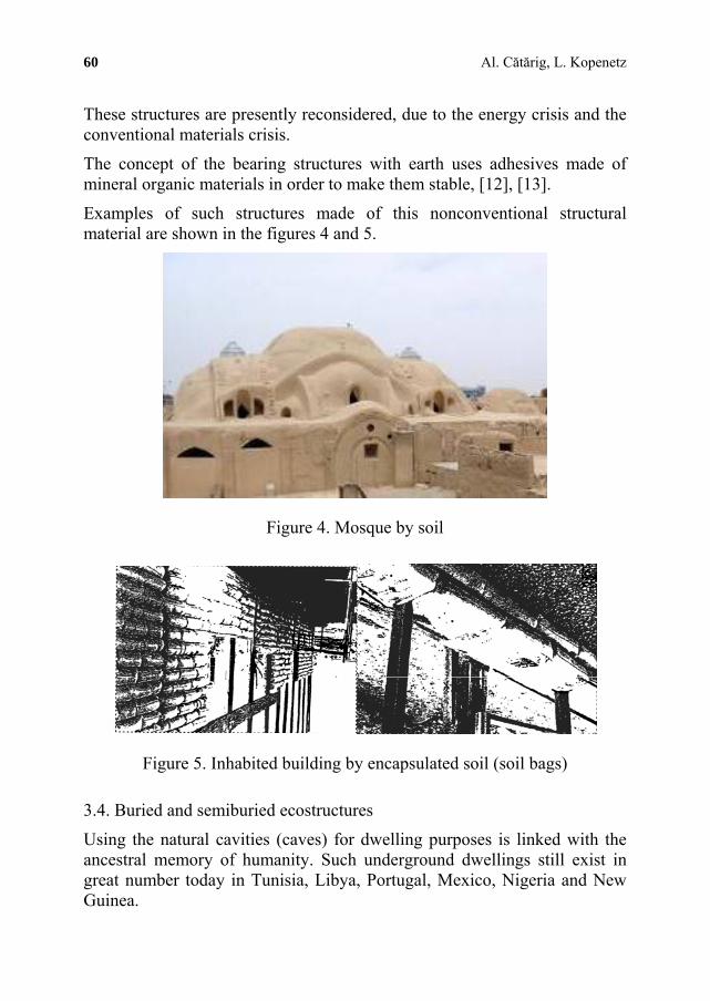
60 Al. Cătărig, L. Kopenetz
These structures are presently reconsidered, due to the energy crisis and the conventional materials crisis.
The concept of the bearing structures with earth uses adhesives made of mineral organic materials in order to make them stable, [12], [13].
Examples of such structures made of this nonconventional structural material are shown in the figures 4 and 5.
Figure 4. Mosque by soil
Figure 5. Inhabited building by encapsulated soil (soil bags)
3.4. Buried and semiburied ecostructures
Using the natural cavities (caves) for dwelling purposes is linked with the ancestral memory of humanity. Such underground dwellings still exist in great number today in Tunisia, Libya, Portugal, Mexico, Nigeria and New Guinea.

“Computational Civil Engineering 2010”, International Symposium 61
The problem of the artificial underground structures resurfaced during the 20th century, both as simple air-raid shelters and as underground towns, deeply buried, used as anti-atomic shelters.
The problem of the underground dwellings also resurfaced due to the worsened situation of the fossil energy use as well as due to the possibility of better anti-seismic protection (Fig.6).
Figure 6. Semi-buried houses
In this context, the advantages of the underground ecostructures are as follows, [14]: - the energetic efficiency and the thermal comfort (coolness during summer and warmth during winter), which means that the energy consumption is reduced by 90% for the buried structures and by 80% for the semiburied dwellings, - anti-seismic protection, - protection against fire, - protection against extreme winds (hurricanes, typhoons).
3.5. Ecostructures with air jet
The air jet structures (Fig.7) appeared at the beginning of the 20th century, as a Swiss patent, having as main components the following three: - the inlet, - the ventilator, - the delivery hose.
According to the direction of the air jet, we can have structures with horizontal flow, tilted flow or vertical flow.
The main advantage of this kind of structures is that they exist and consume energy only for the length of time they actually function or are used.

62 Al. Cătărig, L. Kopenetz
Figure 7. Air jet echostructure
One of the first ecostructures which observes the ecological concepts of our days is the Pantheon in Rome (123 AD) (Fig.8).
Figure 8. Roma’s Pantheon

“Computational Civil Engineering 2010”, International Symposium 63
The design of the construction (the name of the real architect is still uncertain, many asign it to Apollodoros of Damascus) provided an enormous dome with a 9 m opeion. It is mentioned that in the area of the opeion it DOES NOT rain even during heavy rain periods. This is explained by the fact that a natural vertical air flow exists and it makes an immaterial ecological structure in the area of the opening.
Such phenomena have also been seen in cooling towers with natural draught (Fig.9).
Figure 9. Cooling tower, Doel, Belgium
The production of highly efficinet silent engines (for instance magnetic engines) sets the bases for realizing gigantic ventilators which can cover auditoriums, theatres, stadiums, and even civil buildings, in this way reducing significantly the consumption of deficient polluting materials and the financial effort.
In the Orient these structures circumscribe to the FENG SHUI philosophy. This name translates by “WIND and WATER” and has been used for centuries to regulate the energetic levels in the dwellings, without the need of any investment.
The basic principle of this energy regulation lies in performing certain openings, apparently non structural, which will form air and energy flows, in order to dissipate the bad energy. These openings are done empirically and are used even in present days constructions.
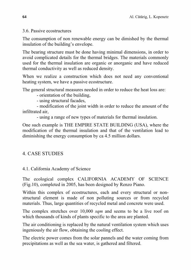
64 Al. Cătărig, L. Kopenetz
3.6. Passive ecostructures
The consumption of non renewable energy can be dimished by the thermal insulation of the building’s envelope.
The bearing structure must be done having minimal dimensions, in order to avoid complicated details for the thermal bridges. The materials commonly used for the thermal insulation are organic or anorganic and have reduced thermal conductivity as well as reduced density.
When we realize a construction which does not need any conventional heating system, we have a passive ecostructure.
The general structural measures needed in order to reduce the heat loss are: - orientation of the building, - using structural facades, - modification of the joint width in order to reduce the amount of the infiltrated air, - using a range of new types of materials for thermal insulation.
One such example is THE EMPIRE STATE BUILDING (USA), where the modification of the thermal insulation and that of the ventilation lead to diminishing the energy consumption by ca 4.5 million dollars.
4. CASE STUDIES
4.1. California Academy of Science
The ecological complex CALIFORNIA ACADEMY OF SCIENCE (Fig.10), completed in 2005, has been designed by Renzo Piano.
Within this complex of ecostructures, each and every structural or non-structural element is made of non polluting sources or from recycled materials. Thus, large quantities of recycled metal and concrete were used.
The complex stretches over 10,000 sqm and seems to be a live roof on which thousands of kinds of plants specific to the area are planted.
The air conditioning is replaced by the natural ventilation system which uses ingeniously the air flow, obtaining the cooling effect.
The electric power comes from the solar pannels and the water coming from precipitations as well as the sea water, is gathered and filtered.

“Computational Civil Engineering 2010”, International Symposium 65
Figure 10. California Academy of Science
4.2. Partially buried buildings
For severe climatic and seismic regions Peter Wetsh (Wetsh Architectures) advances the idea of partially or totally buried houses.
These completely ecological structures usually are in perfect accord with the environment (the relief, the climate).
Figure 11 shows designs illustating this idea, done by students of the Civil Engineering Department in Cluj-Napoca.
Figure 11. Semi-buried complex housing

66 Al. Cătărig, L. Kopenetz
The natural lighting system was solved by a number of spot lights which will direct the natural light, throughout the day, towards the underground area, not accessible to the sun rays (Fig.12÷14), [15], [16], [17].
Figure 12. Semi-buried house type A - Axonometric
Figure 13. Semi-buried house type A - Cross section

“Computational Civil Engineering 2010”, International Symposium 67
Figure 14. Semi-buried house type B - Axonometric and Cross section
5. CONCLUSIONS
- The concepts of eco-architecture and ecostructural engineering must be regarded as the source for principles and measures which will determine the future of the mankind, [18], [19].
- The ecostructures are structures made with reduced energy consumption and they use little natural resources when they function.
- Promoting the ecostructures with all their components (site of the construction, materials used etc.), is the foundation of the preservation of the ecosystem.
- The ecostructures are considered to be the answer to both the energy crisis and the conventional materials crisis.

68 Al. Cătărig, L. Kopenetz
- Approaching the ecostructures is an endeavour of the specialists to find important new directions for the research to benefit the society, to new paths and progress.
- By using the classical structural principles, the ecostructures made of non-conventional materials can meet the ecological requirements, without significant costs, as compared to the structures made of traditional materials. Thus, using the earth structures allows diminishing the energy consumption as well as material consumption, detrimental to the human health, while sustaning the comfort and hygiene requirements in the present times.
References
1. Cătărig, A., Kopenetz, L., Construcţii textile. Prezent şi viitor. Analele Universităţii din Oradea, Tom I, 1998. (in Romanian)
2. Cătărig, A., Kopenetz, L., Hodişan, T., Immaterial Structures in Real Structures, Proceedings of the XXX IAHS World Congress on Housing, vol. 1, Coimbra (Portugal), 2002.
3. Kopenetz, L., Cătărig, A., Reabilitarea structurilor de construcţii cu materiale textile. Lucrările Conferinţei naţionale CisC 2000, Iaşi, 2000. (in Romanian)
4. Kopenetz, L., Cătărig, A., Teoria structurilor uşoare cu cabluri şi membrane, Ed. U.T. PRES, Cluj-Napoca, 2006. (in Romanian)
5. Kopenetz, L., Ionescu, A., Lightweight Roof for Dwellings, International Journal for Housingand its Aplication, vol. 9, no. 3, Miami (Florida), 1985.
6. Lanczos, K., Space Through the Ages, Academic Press Inc., London, 1970. 7. Jammer, M., Concepts of Space, Harvard University Press, Harvard, 1954. 8. Salvadori, M., Building, the Fight Against Gravity, Atheneum, New York, 1979. 9. Balassa, J., Ortutay, G., Ungarische Volkskunde, Ethnographia, Budapest, 1977. 10. Fauth, W., Der Practische Lehmbau, Springer Verlag, Wiesbaden, 1946. 11. McCann, J., Clay and Cob Buildings, Aylesbury, England, 1983 12. Volhard, F., Leichtlehmbau, Universitat Karlsruhe, Karlsruhe, 1983. 13. Gernot, M., Earth Construction Handbook, Wit Press, Southampton, Boston, 2000. 14. Mureşan, Ioana, Mureşan, F., Sisteme de ecoarhitectură – Locuinţe semiîngropate, Lucrările
Sesiunii ştiinţifice Construcţii-Instalaţii CIB 2008, vol.1, Braşov, 2008. (in Romanian) 15. Zoloiu, Luiza, Zimbru, Delia, Bal, R., Proiect de diplomă (Licenţă) – Coordonator prof. L.
Kopenetz, Universitatea Tehnică, Cluj-Napoca, 2009. (in Romanian) 16. Szabo, G., Die Grundlagen Einer Neuen Festigeitstheorie, Springer Verlag, Wiesbaden, 1971. 17. Scheck, F., Mechanics, Springer Verlag, Berlin, Heidelberg, New York, 1990. 18. Goering, P.L.E., Comunicări personale, Toronto, Canada, 1983. 19. Kopenetz, L., Cătărig, A., Ţeserea pământului ca metodă nouă de consolidare a drumurilor,
Lucrările tehnico - ştiinţifice ale celui de al XII-lea Congres Naţional de Drumuri şi Poduri, Tema strategică 4: Calitatea infrastructurilor rutiere, Bucureşti, 2006. (in Romanian)

“Computational Civil Engineering 2010”, International Symposium Iasi, Romania, May 28, 2010
Nonlinear Modeling of Soil Cohesion Intercept Using Generalized Regression Neural Network
Amir Hossein Alavi1, Amir Hossein Gandomi1,2, Ali Mollahasani3, Azadeh Rashed3
1College of Civil Engineering, Iran University of Science and Technology, Tehran, Iran 2The Highest Prestige Scientific and Professional National Foundation, National Elites Foundation,
Tehran, Iran 3Department of Civil Engineering, Ferdowsi University of Mashad, Mashad, Iran
Summary
In this paper, a new nonlinear model was developed to estimate the soil cohesion intercept (c) using generalized regression neural network (GRNN). The proposed model relates c to the basic soil physical properties including the coarse and fine-grained contents, grains size characteristics, liquid limit, moisture content and soil density. The comprehensive experimental database used for developing the model was established upon a series of unconsolidated-undrained triaxial tests conducted in this study. A parametric analysis was also carried out to evaluate the sensitivity of c to the variations of the influencing parameters. In order to benchmark the proposed model, a nonlinear least squares regression (NLSR) analysis was performed. The results indicate that the developed model is capable of effectively estimating the c values for a number of soil samples. The GRNN model is able to reach a significantly better prediction performance compared with the regression model.
KEYWORDS: Soil cohesion intercept; Soil physical properties; Generalized regression neural network; Nonlinear modeling.
1. INTRODUCTION
One of the most important engineering properties of soil is its ability to resist sliding along internal surfaces within a mass. The stability of structures built on soil depends upon the shearing resistance offered by the soil along the probable surfaces of slippage. The shear strength of geotechnical materials is generally represented by the Mohr-Coulomb theory. According to this theory, the shear strength of soils varies linearly with the applied stress through two shear strength

70 A.H. Alavi, A.H.Gandomi, A. Mollahasani, A. Rashed
components known as the cohesion intercept and angle of shearing resistance. The tangent to the Mohr-Coulomb failure envelopes is represented by its slope and intercept. The slope expressed in degrees is the angle of shearing resistance and the intercept is cohesion [1, 2]. The cohesion intercept and angle of shearing resistance are treated as constants over the range of normal stresses. The values of these empirical parameters for any soil depend upon several factors such as the soil textural properties, past history of soil, initial state of soil, permeability characteristics of soil and conditions of drainage allowed to take place during the test [2]. Figures 1(a) and (b) show the Mohr circles and failure envelopes in terms of the total and effective stresses, respectively. If the cohesion intercept and angle of shearing resistance are determined using the total stresses (Figure 1(a)), they are named as total or undrained cohesion intercept (c) and angle of shearing resistance (). The effective stress is the difference between the total stress and the excess pore water pressure. If the pore water pressures are measured during the test, the effective circles can be plotted as shown in Figure 1(b) and the effective strength parameters (c' and ') are obtained.
Figure 1. Mohr circles and failure envelopes in terms of total and effective stresses [2]
Accurate determination of c is a major concern in the design of different geotechnical structures such as foundations, slopes, underground chambers, and open excavations. This key parameter can be determined either in the field or in the laboratory. The triaxial compression and direct shear tests are the most common tests for determining the c values in the laboratory. The testing procedures of triaxial and direct shear tests have respectively been standardized by ASTM WK3821 [3] and ASTM 6528 [4]. The triaxial test is more suitable for clayey soils. The direct shear test is commonly used for sandy soils and requires simpler test procedure in comparison with the triaxial test. The tests employed in the field include vane shear test or any other indirect method [2, 5].
However, experimental determination of c is extensive, cumbersome and costly. Also, it is not always possible to conduct the tests on every new situation. In order to cope with such problems, numerical solutions have been developed to estimate the strength parameters. The fact that most of the available empirical models are based on limited experimental data rises doubts on their generality. On the other hand, despite the multivariable dependency of soils, such correlations are developed on the basis of only one soil index property. Incorporating simplifying

“Computational Civil Engineering 2010”, International Symposium 71
assumptions into the development of the statistical and numerical methods may also lead to very large errors [6-10].
By extending developments in computational software and hardware, several alternative computer-aided data mining approaches have been developed. The idea is that a pattern recognition system learns adaptively from experience and extracts various discriminators, each appropriate for its purpose. Artificial neural networks (ANNs) [11] are the most widely used pattern recognition procedures. ANNs have successfully been applied to the behavior modeling of many civil engineering problems [10, 12-16]. Recently, Kayadelen et al. [17] developed an ANN model to predict the �' value of soils. An alternative ANN approach, which is based on the data alone to determine the structure and parameters of the model, is known as generalized regression neural network (GRNN) [18]. GRNN is on the basis of nonlinear regression theory and often used as a popular statistical tool for function approximation. Some of the scientific efforts directed at applying GRNN to the civil engineering tasks include predicting capacity of driven piles [19], forecasting chlorine residuals [20], modeling river sediment yield [21], and estimating modal damping of flexible beams [22].
GRNN can substantially be useful in deriving an empirical model for characterizing c by directly extracting the knowledge contained in the experimental data. In this paper, the GRNN technique was utilized to obtain a precise model relating c to several physical properties of soils. The proposed model was developed based on triaxial tests conducted in this study. The paper is organized as follows: Section 2 presents brief descriptions of the ANN and GRNN methods. Section 3 outlines the model development using GRNN and reviews the results. The detailed performance analyses of the proposed models are discussed in Section 4. The results of parametric analysis are given in Sections 5. Finally, concluding remarks are outlined in Section 6.
2. ARTIFICIAL NEURAL NETWORK
Artificial neural networks (ANNs) have emerged as a result of simulation of biological nervous system. The ANN method was founded in the early 1940s by McCulloch and co-workers [23]. The first researches were focused on building simple neural networks to model simple logic functions. At the present time, ANNs can be applied to problems that do not have algorithmic solutions or problems with complex solutions. ANN formulates a mathematical model for a system in which no clear relationship is available between inputs and outputs. Unlike most of available statistical methods, ANNs use the data alone to determine the structure of the model and unknown model parameters. The ability of ANNs to learn by example makes them very flexible and powerful techniques. Thus, this approach

72 A.H. Alavi, A.H.Gandomi, A. Mollahasani, A. Rashed
has widely been applied to solving regression and classification problems in many fields. The ANN structure consists of a large number of interconnected processing elements known as neurons acting as microprocessors. Each of the neurons accepts a weighted set of inputs and responds with an output. At first, a neuron forms weighted sum of the inputs as follows:
bxwnN
iii
1 (1)
where N and wi are respectively the number of elements and interconnection weight of the input vector (xi); and b is bias for the neuron. The knowledge is stored as a set of connection weights and biases. Finally, the output is obtained by passing the sum of the product through an activation function (f) as follows:
bxwfnfN
iii
1 (2)
For nonlinear problems, different functions such as the threshold function, sigmoid function, and the hyperbolic tangent function can be adopted as the activation function. Selection of the activation function depends on the type of the network to be designed. ANNs can be trained to perform a particular function by adjusting the values of connections. These networks are trained to reach from a particular input to a target output. This process is iterated until the network output matches the target. The learning ability of an ANN is dependant to its architecture and applied algorithmic method during the training process. A typical structure and operation of ANNs is shown in Figure 2. A neural network consists of an input layer, at least one hidden layer of neurons and an output layer. The hidden layers map the information contained in the input layer to the output layer. Each of the units can send its output only to the higher layer units and receive inputs from the lower layer [24].
Figure 2. Typical structure of ANNs
“Computational Civil Engineering 2010”, International Symposium 73
2.1. Generalized regression neural network
Generalized regression neural network (GRNN) was first proposed by Specht [18]. GRNN is a class of ANN architectures that does not require an iterative training procedure as in the common back propagation method. GRNN is capable of approximating any function between the input and output vectors based on the training data alone. As the training set size becomes large, the GRNN estimation error nears zero, with only slight restrictions on the function. This method is usually utilized for approximation of continuous variables as in conventional regression techniques. GRNN is one variant of the radial basis function (RBF) network. It is on the basis of a standard statistical technique called Kernel regression. Unlike the standard RBF network, the weights of GRNN networks can be calculated analytically. In GRNN, the training patterns are propagated through the network only once, and thus the training is achieved very quickly [18]. Intrinsically, the regression of a dependent parameter (y) on an independent variable (x) predicts the most probable value for y, given x and training data. This regression technique produces the estimated value of y which minimizes the mean squared error. GRNN is an approach for approximating the joint probability density function of x and y, given only a training set [21].
The system is perfectly general since the probability density function is originated from the data with no presumption about its form. If represents the known joint continuous probability density function of a vector random variable (x) and a scalar random variable (y), the regression of y on X is as given below:
F(X, Y)
dyyXyF
dyyXyFXyE
,
,
(3)
When the density function of is not known, it must commonly be approximated from a sample of observations of x and y. The following probability estimator is based on sample values Xi and Yi of the random variables x and y:
F(X, Y)
(X, Y) F
2
2
12121 2
exp2
exp1
2
1,ˆ
in
i
Tii
dd
YYXXXX
nyXF
(4)
where n is the number of sample observations and d is the dimension of the vector variable x. assigns sample probability of width for each sample Xi and Yi. The probability estimate will be the sum of those sample probabilities [18, 21]. Performing the indicated integrations yields the following equation:
(x, y) F

74 A.H. Alavi, A.H.Gandomi, A. Mollahasani, A. Rashed
n
i
i
in
i
i
D
DY
XY
12
2
2
2
1
2exp
2exp
ˆ
(5)
where,
iTii XXXXD 2 (6)
(X)Y is directly applicable to problems involving numerical data. If the smoothing
parameter () is considered large, the approximated density is forced to be smooth and in the limit becomes a multivariate Gaussian with covariance equal to 2i. Considering a smaller value for allows the estimated density to assume non-Gaussian shapes, but the wild points may have too great effect on the approximations [18]. The GRNN structure is composed of four layers: input layer, pattern layer, summation layer and output layer. A schematic representation of GRNN architecture is shown in Figure 3. The input units are in the first layer. The fist layer comprises the input units, the pattern units are in the second layer. The outputs of the second layer re passed on to the summation units in the third layer. The output units are covered in the fourth layer.
Figure 3. A schematic representation of GRNN architecture

“Computational Civil Engineering 2010”, International Symposium 75
3. GRNN SIMULATION OF SOIL COHESION INTERCEPT
Precise estimation of the cohesion intercept values is an essential criterion in the design process of the geotechnical tasks. Due to complexity of the soil strength parameters behavior, it is not simple to identify a relationship between the involved parameters. Cohesion is mainly due to the intermolecular bond between the adsorbed water surrounding each grain, especially in fine-grained soils [2, 5]. The soils with high plasticity like clayey soils have higher cohesion and lower angle of shearing resistance. Conversely, as the soil grain size increases like sands, the soil cohesion decreases. Therefore, in a rational manner the main parameters which affect the soil cohesion intercept will be the soil type, soil plasticity, and soil density.
The main purpose of this study is to obtain a meaningful relationship between the cohesion intercept (c) and the influencing parameters using the GRNN approach. The most important factors representing the c behavior were detected based on the literature review [2, 5, 17, 25]. c (kg/cm2) was considered to be a function of several parameters as follows:
γ,LL,W,CFC,Dfc, du ,30 (7)
where,
FC (%): Fine-grained content
D30 (mm): Grain size for which 30 percentage of the sample was finer
Cc: Coefficient of curvature ((D30)2 / (D60 D10))
LL (%): Liquid limit
W (%): Moisture content
γd (gr/cm3): Soil dry density
The significant influence of the above parameters in determining c is well understood [2]. The following multi-objective strategy was considered to choose the best GRNN models:
i. Providing the best fitness value on the training set of data.
ii. Providing the best fitness value on a test set of unseen data.
3.1. Performance measures
Correlation coefficient (R), mean squared error (MSE) and mean absolute error (MAE) were used to evaluate the capabilities of the proposed models.

76 A.H. Alavi, A.H.Gandomi, A. Mollahasani, A. Rashed
R, MSE and MAE are given in the form of equations as follows:
21
1
ni itit
ni ititihih
R2
1
ni ihih
(8)
n
nitih
2
iMSE 1 (9)
niMAE 1
nitih
(10)
where hi and ti are respectively the actual and predicted output values for the ith output,
ih is the average of the actual outputs, and n is the number of sample.
3.2. Experimental study
Triaxial compression test is presently the most widely used procedure for determining the shear strength parameters of soils. In the triaxial soil testing system, field conditions can be simulated in a way that surpasses other testing methods. This is due to the fact that the confining pressure is applied to the soil specimen according to the uniform lateral in situ stresses in triaxial testing apparatus. With respect to the problem statement, three types of testing techniques can be applied, namely unconsolidated undrained (UU), consolidated undrained (CU), and consolidated drained (CD) [22]. Within the scope of this study, a series of unconsolidated, undrained, and unsaturated triaxial (UU) tests were performed in accordance with ASTM D2850-87 to determine the shear strength parameters of 81 different undisturbed soil samples.
3.2.1. Sampling
The soil samples were manually taken by divers from test pits at some locations in Khorasan and Khouzestan provinces, Iran, using metal tubes, 4 inch and 6 inch in diameter. After extracting, the cores were carefully taken to the geotechnical laboratory and maintained in a wet chamber, to avoid loosing of water content. Undisturbed sub-samples were then extracted from the cores for the geotechnical characterization tests. Also, several disturbed soil samples were taken from the sites for testing purposes.

“Computational Civil Engineering 2010”, International Symposium 77
3.2.2. Basic geotechnical characterization tests
Extensive geotechnical laboratory test programs were carried out for the basic characterization of soils. These comprised classification tests; water (or moisture) content, defined as the ratio between the mass of water and the mass of dry soil; natural unit weight of the soil, which is obtained by measuring the relationship between the weight and volume of an undisturbed soil sample; Atterberg limits (plastic and liquid limits) and grain size distribution. The grain size distribution of the disturbed samples was determined by sieving from number 4, 8. 16, 30, 50, 100 and 200 sieves and for finer soils (silt and clay) remaining from the 200 sieves. A sedimentation test throughout a hydrometer analysis was also carried out. To avoid flocculation of the finer fraction, a dispersing agent (sodium hexametaphosfate) was added to the soil-water mixture before the sedimentation test. Figure 4 illustrates the range of grain size distribution of the samples tested.
Figure 4. Grain size distributions of soil samples
3.2.3. Triaxial compression tests
The soils taken at depth ranging from 30 m to 5 m and contain no gravel or larger particles. The soil samples with dimension of 38-50 mm in diameter and 76-100 mm in height were used in the unconsolidated undrained triaxial tests. The samples were enclosed in a thin rubber membrane and closed tightly using plastic O-rings from the top platen and base pedestal. Then, they were placed inside the water-filled cell. Afterwards, a known magnitude of confining pressure of the fluid was applied inside the cell. In order to obtain the soil failure, an axial stress was implemented on the top of the soil specimen by a frictionless ram through the top of the cell. Meanwhile, the axial stress applied and axial displacement of samples were measured by load cell until the samples fails. This test was repeated at least for three confining pressures. The database includes measurements of fine (FC) and coarse-grained (CC) contents, the grain size, in millimeters, for which 30 percentage of the sample was finer (D30), coefficient of uniformity (Cu),

78 A.H. Alavi, A.H.Gandomi, A. Mollahasani, A. Rashed
percentages of liquid limit (LL) and moisture content (W), bulk density (γ), and dry density (γd). c was also measured as one of the soil shear strength parameters. Total of 81 data sets were considered for developing the prediction models. A major part of the database comprises the laboratory test results on fine-grained soil samples.
3.3. Data preprocessing
Some of the soil property variables are fundamentally interdependent. The first step in the analysis of interdependency of the data is to make a careful study of what it is that these variables are measuring, noting any highly correlated pairs. High positive or negative correlation coefficients between the pairs may lead to poor performance of the models and difficulty in interpreting the effects of the explanatory variables on the response. This interdependency can cause problems in analysis as it will tend to exaggerate the strength of relationships between variables. This is a simple case commonly known as the problem of multicollinearity. Thus, the correlation coefficients between all possible pairs were determined. The correlation coefficients between the pairs are shown in Table 1.
Table 1. Correlation coefficients between all pairs of the explanatory variables Variable FC (%) CC (%) D30 (mm) Cu LL (%) γ (gr/cm3) W (%) γd (gr/cm3)
FC (%) 1.000 -1.000 -0.559 -0.250 0.032 0.153 0.310 -0.045
CC (%) -1.000 1.000 0.559 0.250 -0.032 -0.153 -0.310 0.045
D30 (mm) -0.559 0.559 1.000 0.014 0.138 -0.119 -0.242 0.038
Cu -0.250 0.250 0.014 1.000 -0.040 0.140 0.083 0.116
LL (%) 0.032 -0.032 0.138 -0.040 1.000 0.099 0.150 0.017
γ (gr/cm3) 0.153 -0.153 -0.119 0.140 0.099 1.000 0.594 0.802
W (%) 0.310 -0.310 -0.242 0.083 0.150 0.594 1.000 -0.002
γd (gr/cm3) 0.310 0.045 0.038 0.116 0.017 0.802 -0.002 1.000
As can be seen in this table, there is a high negative correlation between FC and CC in the operation. This is apparent since CC is calculated by subtracting FC from 100. Also, the correlation coefficient between γ and γd is high. Since there will be no advantage of having both variables in the modeling (one can represent the other), decisions were made to remove the correlated parameters in order to maximize the reliability of the final model. The descriptive statistics of the data used in this study are also given in Table 2.

“Computational Civil Engineering 2010”, International Symposium 79
Table 2. Descriptive statistics of the variables used in the model development Parameter FC (%) CC (%) D30 (mm) Cu LL (%) γ (gr/cm3) W (%) γd (gr/cm3) c (kg/cm2)
Mean 80.945 0.051 78.543 28.171 16.643 1.607 0.367 80.945 0.051
Standard Error 2.112 0.026 20.083 0.634 0.637 0.012 0.031 2.112 0.026
Median 87.750 0.014 28.286 27.000 16.350 1.620 0.320 87.750 0.014
Mode 94.400 0.020 30.000 27.000 20.000 1.550 0.370 94.400 0.020
Standard Deviation 19.124 0.239 181.858 5.739 5.765 0.109 0.284 19.124 0.239
Sample Variance 365.724 0.057 33072.273 32.933 33.234 0.012 0.081 365.724 0.057
Kurtosis 3.184 49.371 22.372 1.204 0.046 -0.686 0.514 3.184 49.371
Skewness -1.731 6.918 4.539 1.256 0.009 -0.192 0.961 -1.731 6.918
Range 89.50 1.899 1147.86 26.00 26.50 0.44 1.14 89.50 1.899
Minimum 9.60 0.001 2.14 20.00 3.50 1.37 0.02 9.60 0.001
Maximum 99.10 1.900 1150.00 46.00 30.00 1.81 1.16 99.10 1.900
Sum 7206.67 1593.33 4.308 6390.16 2411.00 164.41 1448.15 141.15 31.98
3.4. Model development using GRNN
The available database was used for generating the GRNN prediction models. After developing and controlling different models with different combinations of the input parameters, the final explanatory variables (FC, D30, Cu, LL, W, γd) were selected as the inputs of the optimal model. Thus, the proposed GRNN model had three layers: six input units (FC, D30, Cu, LL, W, and γd) in the input layer, a hidden layer with 62 neurons (equal to the number of training data), and an output layer (c). For the development of GRNN model, a script was written in the MATLAB environment using Neural Network Toolbox 5.1 [26]. In order to avoid overtraining, the spread of the radial basis functions (spread constant) was changed in away that error of the testing data became close to error of the training data sets [27]. If a smaller spread constant was selected, the output of models would completely fit on training data, but the generalization ability of the models might be decreased.
For the GRNN analysis, the data sets were randomly divided into training and testing subsets. Training data were used for learning. The testing data were used to measure the performance of the GRNN models on data that played no role in building the models. Out of 81 data for the prediction of c, 61 (75%) data vectors were used for training and 20 (25%) data for testing the models. In order to obtain a consistent data division, several combinations of the training, validation and testing sets were considered. The selection was such that the maximum, minimum, mean and standard deviation of parameters were consistent in the data sets. Both input and output variables were normalized in this study. After controlling several

80 A.H. Alavi, A.H.Gandomi, A. Mollahasani, A. Rashed
normalization methods [29, 30], the following method was used to normalize the variables to a range of [U, L]:
= ax + b X n (11)
where,
minmax X-X
L-U = a
(12)
maxaX- U= b (13)
in which Xmax and Xmin are the maximum and minimum values of the variable and Xn is the normalized value. In the present study, U = 0.95 and L = 0.05. Comparisons of the GRNN predicted versus experimental c values are shown in Figure 5.
Figure 5. Predicted versus experimental c values using the best GRNN model: (a) training data, (b) testing data
3.5. Model development using regression analysis
A multivariable nonlinear least squares regression (NLSR) [31] analysis was performed to have an idea about the predictive power of the best GRNN model, in comparison with a classical statistical approach. The method of NLSR is extensively used in regression analysis primarily because of its interesting nature. Under certain assumptions, NLSR has some attractive statistical properties that have made it as a member of the most powerful and popular methods of regression analysis. NLSR extends linear least-squares regression for use with a much larger and more general class of functions. Unlike linear regression models, there are very few limitations on the way parameters can be used in the functional part of

“Computational Civil Engineering 2010”, International Symposium 81
nonlinear regression models (Ryan 1997). The major task was to determine the NLSR-based equation connecting the input variables to the output variable as:
1311975303112108642 aaWαLLαCαDαFCαc a
daαα
uαα (14)
where a denotes coefficient vector. The NLSR model was trained using the same training and testing data sets previously considered for developing the GRNN models. Eviews software package [32] was used to perform the regression analysis. Formulation of c, in terms of the independent variables, FC, D30, Cu, LL, W, and γd, for the best result by the NLSR analysis, is as given below:
219.62163.0927.119
788.1500009.000000005.0221.90cmkg985.2003.0
005.0804.0781.2530
002.02
d
uNLSR
W
LLCDFCc
(15)
Comparisons of the NLSR predicted versus experimental c values are shown in Figure 6.
Figure 6. Predicted versus experimental c values using the NLSR model: (a) training data,
(b) testing data
4. PERFORMANCE ANALYSIS OF THE MODELS
A precise model for the soil cohesion intercept was developed upon a reliable database. No rational models for the prediction of c have been found that encompass the influencing variables considered in this study. Thus, it was not possible to conduct a comparative study between the results of this research and those in hand. Based on a logical hypothesis [33, 34], if a model gives R > 0.8, and the error (e.g., MSE and MAE) values are at the minimum, there is a strong correlation between the predicted and measured values. The model can therefore be

82 A.H. Alavi, A.H.Gandomi, A. Mollahasani, A. Rashed
judged as very good. It can be observed from Figure 5 that the GRNN model with high R and low MSE and MAE values is able to predict the target values to an acceptable degree of accuracy. The minimum ratio of the number of objects over the number of selected variables for model acceptability is 3, but often a suffer value of 5 is suggested [28]. In the present study, this ratio is much higher and is at least equal to 82/5 = 16.4. The above facts ensure that the GRNN model is valid and has the prediction power and is not a chance correlation. It is obvious that, in all cases, the GRNN model has remarkably better performance in comparison with the NLSR model. Empirical modeling based on statistical regression techniques has significant limitations. Most commonly used regression analyses can have large uncertainties, which own major drawbacks pertaining idealization of complex processes, approximation and averaging widely varying prototype conditions. In regression analyses, the nature of corresponding problem is tried to be modeled by a pre-defined equation, either linear or nonlinear.
Besides, Figure 7 shows the ratios of the experimental c values to the values predicted by the GRNN model with respect to FC, D30, Cu, LL, W, and γd. The results indicate that the scattering slightly increases when FC increases and it decreases with increasing D30, Cu, and LL. In all of the cases, the trends are not significant with respect to the design parameters, in particular for W and γd. This confirms the acceptable accuracy of the proposed model.
Figure 7. The ratio between the predicted and experimental c values with respect to the design parameters

“Computational Civil Engineering 2010”, International Symposium 83
5. PARAMETRIC ANALYSIS
For further verification of the GRNN model, a parametric analysis was performed in this study. The main goal is to find the effect of each parameter on the c values. Figure 8 presents the tendency of the c predictions to the variations of the soil physical properties, FC, D30, Cu, LL, W, and γd.
Figure 8. Parametric analysis of the soil cohesion intercept in the GRNN model
The results of parametric analysis indicate that c continuously increases when FC and D30 decrease respectively up to 40 % and 0.7 mm and thereafter it starts increasing. c increases when Cu increases up to 500 and for larger values of Cu, it starts decreasing. The results indicate that c increases with increasing LL and γd, and decreases when W increases. The parametric analysis results are generally expected cases from a geotechnical engineering viewpoint [2].

84 A.H. Alavi, A.H.Gandomi, A. Mollahasani, A. Rashed
6. CONCLUSIONS
In this research, a high-precision model was derived for assessing the soil cohesion intercept, c, using the GRNN method. The proposed model was developed based on well established and widely dispersed triaxial test results obtained through an experimental study performed in this study. A nonlinear regression analysis was performed to have an idea about the predictive power of the GRNN model. The following principal conclusions may be drawn based on the results presented:
The developed GRNN model gives reliable estimates of the c values. The results indicate that the proposed model possesses some obvious superiority in comparison with the developed regression model.
The proposed model simultaneously takes into account the role of several important factors (FC, D30, Cu, LL, W, and γd) representing the behavior of shear strength parameters. Contrary to the conventional models that are based on only one soil index property, the proposed model handles all different cases of the soil type, soil plasticity, and soil density.
The proposed model is mostly suitable for fine-grained soils. By adding newer data sets for other soil types and test conditions, this model can be improved to make more accurate predictions for a wider range.
The parametric analysis results are mostly expected cases from a geotechnical engineering viewpoint. The results confirm the robustness of the developed GRNN model.
With the use of the GRNN approach, the c values can be estimated without carrying out sophisticated and time-consuming laboratory or field tests.
Unlike the other well known ANN architectures such as back propagation method, GRNN does not require an iterative training procedure [21]. This results in a significant speedup in the GRNN algorithm training process.
By distributing the GRNN model as a code for predicting the c values, other investigators will be able to use this approach.
References
1. Arora, K.R., Introductory soil engineering, text book., Delhi, Nem Chand Jane (Prop.), Standard Publishers Distributors, 1988.
2. Murthy, S., Geotechnical Engineering: Principles and Practices of Soil Mechanics, UK, CRC Press, 2008.
3. ASTM WK3821, New test method for consolidated drained triaxial compression test for soils. 4. ASTM D 6528, Consolidated undrained direct simple shear testing of cohesive soils.

“Computational Civil Engineering 2010”, International Symposium 85
5. El-Maksoud, M.A.F., Laboratory determining of Soil Strength Parameters in Calcareous Soils and Their Effect on Chiseling Draft Prediction, In: Energy Efficiency and Agricultural Engineering International Conference, Rousse, Bulgaria, 2006.
6. Bowles, J.E., Engineering properties of soils and their measurement (Fourth ed.), New York, NY, McGraw-Hill, 1992.
7. Korayem, A.Y., Ismail K.M., Sehari, S.Q., Prediction of soil shear strength and penetration resistance using some soil properties, Missouri journal Agricultural Research, vol. 13(4), 1996.
8. Panwar. J.S., Seimens, J.C., Shear strength and energy of soil failure related to density and moisture, Transactions of the ASAE, vol. 15, 1972.
9. Terzaghi, K., Peck, R.B., Mesri, G., Soil mechanics in engineering practice (2nd ed.), New York, NY: Wiley & Sons, Inc., 1996.
10. Shahin, M.A., Maier, H., Jaksa, M.B., Artificial neural network applications in geotechnical engineering, Australian Geomechanics Journal, vol. 36(1), 2001.
11. Haykins, S., Neural networks – A comprehensive foundation (2nd Ed.), Englewood Cliffs, Prentice Hall Inc., 1999.
12. Alavi, A.H., Gandomi, A.H., Mollahasani, A., Rashed, A., Heshmati, A.A.R., Modeling of Maximum Dry Density and Optimum Moisture Content of Stabilized Soil Using Artificial Neural Networks, Journal of Plant Nutrition and Soil Science, 2010.
13. Alavi, A.H., Gandomi, A.H., Gandomi, M., Sadat Hosseini S.S., Prediction of Maximum Dry Density and Optimum Moisture Content of Stabilized Soil Using RBF Neural Networks, The IES Journal Part A: Civil & Structural Engineering, vol. 2(2), 2009.
14. Dombaycı, Ö.A., The prediction of heating energy consumption in a model house by using artificial neural networks in Denizli–Turkey, Advances in Engineering Software, 2009.
15. Heshmati, A.A.R., Alavi, A.H., Keramati, M., Gandomi, A.H., A Radial Basis Function Neural Network Approach for Compressive Strength Prediction of Stabilized Soil, Geotechnical Special Publication ASCE, vol. 191, 2009.
16. Özcan, F., Atiş, C.D., Karahan, O., Uncuoğlu, E., Tanyildizi, H., Comparison of artificial neural network and fuzzy logic models for prediction of long-term compressive strength of silica fume concrete, Advances in Engineering Software, vol. 40(9), 2009.
17. Kayadelen, C., Günaydın, O., Fener, M., Demir, A., Özvan, A., Modeling of the angle of shearing resistance of soils using soft computing systems, Expert Systems with Applications, vol. 36, 2009.
18. Specht, D.F., A general regression neural network. IEEE Transactions on Neural Networks, vol. 2(6), 1991.
19. Abu Kiefa, M.A., General Regression Neural Networks for Driven Piles in Cohesionless Soils, Journal of Geotechnical and Geoenvironmental Engineering, vol. 124, 1998.
20. Bowden, G.J., Nixon, J.B., Dandy, G.C., Maier, H.R., Holmes, M., Forecasting chlorine residuals in a water distribution system using a general regression neural network. Mathematical and Computer Modelling, vol. 44(5-6), 2006.
21. Cigizoglu, H.K., Alp, M., Generalized regression neural network in modelling river sediment yield, Advances in Engineering Soft, vol. 37, 2006.
22. Tanrikulu, A.H., Application of ANN techniques for estimating modal damping of impact-damped flexible beams, Advances in Engineering Soft, vol. 40, 2009.
23. Perlovsky, L.I., Neural networks and intellect, Oxford University Press, 2001. 24. Yilmaz, M., Ertunc, H.M., The prediction of mechanical behavior for steel wires and cord
materials using neural networks, Mater Design, vol. 28, 2007. 25. Barends, F.B.J., Lindenberg, J.L., De Quelerij, L., Verruijt, A., Luger, H.J., Geotechnical
Engineering for Transportation Infrastructure: Theory and Practice, Planning and Design, Construction and Maintenance, Netherlands, Balkema Publishers, 1999.
26. MathWorks, MATLAB the language of technical computing, Version 7.4, USA, Natick, MA, 2007.
27. Bagherieh, A.H., Hower, J.C., Bagherieh, A.R., Jorjani, E., Studies of the relationship between petrography and grindability for Kentucky coals using artificial neural network, International Journal of Coal Geology, vol. 73, 2008.

86 A.H. Alavi, A.H.Gandomi, A. Mollahasani, A. Rashed
28. Frank, I.E., Todeschini, R., The data analysis handbook, Amsterdam, Elsevier, 1994. 29. Swingler, K., Applying neural networks a practical guide, New York, Academic Press, 1996. 30. Mesbahi, E., Application of artificial neural networks in modelling and control of diesel engines,
PhD Thesis, University of Newcastle upon Tyne; 2000. 31. Ryan, T.P., Modern Regression Methods. New York (NY), Wiley, 1997. 32. Maravall, A., Gomez, V., Eviews Software, Version5, Irvine CA, Quantitative Micro Software,
LLC, 2004. 33. Smith, G.N. ,Probability and statistics in civil engineering. London: Collins; 1986. 34. Kasabov, N.K., Foundations of neural networks fuzzy systems and knowledge engineering, MIT
Press, Cambridge, 1998.

“Computational Civil Engineering 2010”, International Symposium Iasi, Romania, May 28, 2010
Static nonlinear analysis of structural reinforced concrete walls energy dissipators with shear connections
Sergiu Andrei Băetu1, Ioan Petru Ciongradi1, Georgeta Văsieş2 1Department of structural mechanics, ”Gheorghe Asachi” Technical University, Iaşi, Zip
code:700050, Romania 2Department of civil and industrial engineering, ”Gheorghe Asachi” Technical University, Iaşi, Zip
code:700050, Romania
Summary
Structural reinforced concrete walls are a structural system that provides lateral resistance, high stiffness and strength to a building. Because the energy dissipation is made only by the base of the structural walls, they do not exhibit ductile and redundant behavior. The structural reinforced concrete wall energy dissipator named and structural slit wall with shear connections remove some of the problems encountered with ordinary structural walls. Yielding of shear connections in this wall may cause increase in energy dissipation, forming a structural damper that is based on structural passive control.
In this paper, the static nonlinear analysis on energy dissipator wall with shear connectors is done and the influence of the elasto-plastic behavior of the shear connections is evaluated. This type of structural wall is compared to an ordinary solid wall. In order to obtain the optimal control effect, the stiffness and strength of the energy dissipation device should be optimized by selecting the dimensions and the number of the shear connections.
The objective of this solution is to create an ideal structure for tall multi-storey buildings, that behaves as a rigid structure at low seismic action and turns into a flexible one in case of a high intensity earthquake action.
KEYWORDS: structural reinforced concrete walls energy dissipators, pushover analysis, ductile behavior, shear connections.

88 S. Băetu, P. Ciongradi, G. Văsieș
1. INTRODUCTION
Reinforced concrete walls are strength elements frequently used in construction in seismic areas, because they have a high lateral stiffness and resistance to external horizontal loads.
If the wall stiffness is high, the seismic loads taken by the structure become heigher, resulting non-economic sections for the wall. This phenomenon occurs particularly in multi-storey tall buildings. In case of high intensity earthquakes flexible structures are preferred because can accept large deformations, instead for low intensity earthquakes that occur frequently, or for wind action, rigid structures should be considered, because prevent large displacements. The dissipation of the accumulated energy in the stuctural wall systems occurs generally through concentrated degradation at the base of the wall, which is difficult to repair. Numerous investigations have been made to improve redundancy and ductility of structural walls exposed to horizontal actions and some practical solutions were proposed. Slit walls are a special variant of structural walls with improved ductility. The specialists intention was to reduce the degradation from the base of the wall and distribute it on the wall height.
First reinforced concrete structural wall, with good properties of seismic energy dissipation, called slit wall was patented by Professor K. Muto in Japan in 1973 (Figure 1) [1]. These walls are the first energy dissipation system used in the structures of Japan.
Figure 1. Slitted panels

“Computational Civil Engineering 2010”, International Symposium 89
The structural reinforced concrete energy dissipator wall with shear connections is first analyzed by researchers from Chinese University of Hong Kong (Figure 2) [2]. Reinforced concrete connections were placed on the slit height which attach the structural walls forming a dissipative zone.
Figure 2. Slit wall with shear connections
It is designed in such a way that under normal wind and earthquakes, the shear connections would remain elastic so that the structural slit wall behaves like a solid wall but when overloaded due to earthquake attack, the shear connections would yield thereby decreasing the lateral stiffness and increasing the damping capacity of the structural system. Although the shear connections would be damaged after yielding, their sacrifice would help to protect the wall itself, which is very dificult to repair. Seismic performance depends on the yielding resistance of the connections. An efficient design of these systems must take into account a rational design of the connectors. The premature yielding of the connectors must be avoided and also the destruction of walls without yielding of the connectors.

90 S. Băetu, P. Ciongradi, G. Văsieș
2. STRUCTURE DESCRIPTION
The building is located in Jassy with site characteristics: design ground acceleration ag =0.2g, control period Tc=1.6s, ductility class H, importance factor γI=1 [3]. It was considered a dual reinforced concrete structure, with regular form in plan and elevation. Seismic lateral loads are taken by the concrete core and by the border walls of the building disposed on short direction. The building has 20 levels resulting a height of 60 m, each level has a height of 3m. The concrete from critic zone is BC30/40. Fundamental period of the structure is T1=1.077s. The investigation focused on the research of a lateral wall with length of 10m. The design analysis was achieved in ETABS Nonlinear, resulting that the thickness wall is 40 cm and is reinforced with vertical bars Φ14/15 and horizontal bars Φ10/15[4].
Figure 3. Building plan Figure 4. 3d view
3. METHOD OF ANALYSIS
3.1 Equivalent frame method
The equivalent frame method is used to design slit walls with reinforced concrete short connections [2]. Structural walls are modeled as columns and connections are modeled as flexible beams in slit region and as infinite rigid beams in the wall

“Computational Civil Engineering 2010”, International Symposium 91
region (Figure 5). For the analysis of the structural system a standard frame program is used. In the analysis the nonlinear inelastic behavior of the connections is considered such as for the base columns.
Figure 5. Equivalent frame method for slit wall with shear connections
3.2 Verification of structural modelling
The equivalent frame analogy adopted for modelling the slit wall structures has the advantages of being simple, easy to understand and fast to analyze as compared to the more sophisticated finite element method. Its advantages are even more pronounced in nonlinear static and dynamic analysis as the structure has to be analyzed again and again many times. Before proceeding to pushover analysis, the applicability of the structural model is first verified by checking its structural analysis results with those obtained by the more rigorous finite element method. The reinforced concrete structural wall extracted from the 20 storey structure proposed in this paper with one central band of vertical slits is analyzed. The height of each connection is 0.6 m and the thickness of the slit is 4 cm (Figure 6).
The equivalent static lateral seismic load is calculated with relation:
Fb = c ˖ G (1)
11
( )ga Tc
g q
(2)

92 S. Băetu, P. Ciongradi, G. Văsieș
Fb – base shear;
ag=0.2g – design base acceleration for seismic zone Jassy;
β(T1)= β0=2.75, for T1<Tc – normalized elastic response spectrum;
λ=0.85 – correction factor;
q=1 – behavior factor for an elastic response;
The gravity loads include slit wall weight and loads from floor connected to the wall resulting a total force of 11180 kN. The total lateral load applied is 5226.7 kN.
The base shear is distributed linear on height of the wall with relation:
1
i ii b n
i ii
G zF F
G z
(3)
The analytical results of the equivalent frame analogy and those obtained by a standard finite element analysis in Etabs Nonlinear are compared in Table 1. It is seen from the comparison that the difference between the numerical results obtained by the present method and the finite element method is generally of the order of only 2..3%. Hence, the idealized structural model should be suficiently accurate for the analysis of reinforced concrete structural slit walls.
Figure 6. Slit wall analyzed
Table 1. Comparison with finite element analysis results Method of analysis Equivalent frame method Finite element method
Top displacement (cm) 18,52 18,53 Fundamental period T1 (s) 0,8435 0,8433
P1 30692.3 30994.35 Axial force at base of wall (kN) P2 -30692.3 -30994.35 P1 2629.46 2636.65 Shear at base of wall (kN) P2 2620.54 2613.35 P1 30609.52 29883.31 Moment at base of wall (kN˖m) P2 30565.16 29775.06

“Computational Civil Engineering 2010”, International Symposium 93
3.3 Pushover analysis with ETABS Nonlinear [5]
The pushover analysis of a structure is a static non-linear analysis under permanent vertical loads and gradually increasing lateral loads. The equivalent static lateral loads approximately represent earthquake induced forces. A plot of the total base shear versus top displacement in a structure is obtained by this analysis that would indicate any premature failure or weakness. The analysis is carried out up to failure, thus it enables determination of collapse load and ductility capacity. Static pushover analysis is an attempt by the structural engineering profession to evaluate the real strength of the structure and it promises to be a useful and effective tool for performance based design.
The ATC-40 [6] and FEMA-237 [7] documents have developed modeling procedures, acceptance criteria and analysis procedures for pushover analysis. These documents define force-deformation criteria for hinges used in pushover analysis. As shown in Figure 7, five points labeled A, B, C, D, and E are used to define the force deflection behavior of the hinge and three points labeled IO, LS and CP are used to define the acceptance criteria for the hinge (IO, LS and CP stand for Immediate Occupancy, Life Safety and Collapse Prevention respectively) [5].
Figure 7. Hinge nonlinear curve
The Etabs Nonlinear static pushover analysis capabilities, which are fully integrated into the program, allow quick and easy implementation of the pushover procedures prescribed in the ATC-40 and FEMA-237 documents for both two and three-dimensional structures. Hinges can be assigned at any number of locations along the length of any frame element. Uncoupled moment, torsion, axial force and shear hinges are available. There is also a coupled P-M2-M3 hinge that yields based upon the interaction of axial force and bending moments at the hinge location. It must be emphasized that the pushover analysis is approximate in nature and is based on static loading. As such it cannot represent dynamic phenomena with a large degree of accuracy. It may not detect some important deformation modes that may occur in a structure subjected to severe earthquakes, and it may exaggerate others. Inelastic dynamic response may differ significantly from

94 S. Băetu, P. Ciongradi, G. Văsieș
predictions based on invariant or adaptive static load patterns, particularly if higher mode effects become important.
4. PUSHOVER ANALYSIS FOR DIFFERENT TYPE OF WALLS
Pushover analysis was performed on several types of constructive solutions for the structural slit wall proposed in this paper. In order to obtain the optimal control effect, the stiffness and strength of the energy dissipation device should be optimized by selecting the dimensions and number of the shear connections. These types of structural walls are compared to an ordinary solid wall with the same dimensions [8] [9].
4.1 Shear connections height variation
Heights of connections are: 0.2 m; 0.4 m; 0.6 m; 0.8 m; 1 m; 1.6 m.
Figure 8 shows the load-lateral displacement diagram at the roof so as to investigate level dissipation and ductility for the structural walls analyzed. Comparisons between pushover curves shows influence of shear connections height on ductility. It has been found from these studies that in most structural slit walls, plastic hinges are formed on the shear connections before the walls fail and that such plasticization can substantially increase the ductility of the structures. Within certain limits, the earlier the shear connections start to yield, the greater will be the increase in ductility. However, if the connections yield prematurely, the lateral strength of the wall structures might be severely affected and the ductility of the connections might become exhausted when the walls start yielding. Thus for best performance, the shear connections should yield before the walls do, but not so early as to cause excessive reduction in lateral strength or breakage of the connections before the walls fail.
The ductility and the behavior factor for the structural slit walls analyzed are given in the Table 2. Comparison of these parameters can reveal the weakness and strong points of different types of structural walls against lateral loads. The ductility factor, μ = du/dy is obtained using the pushover curves from Figure 8, where du – is ultimate displacement and dy – represent yielding displacement of structural walls.
The behavior factor is obtained using equation: y u
u y
V dq
V d , where Vy – is lateral
load at the beginning of yielding and Vu – is ultimate lateral force for the structural walls [10]. The higher the ductility is, the structural system has a greater potential for energy dissipation. For best performance, the connecting beams should maintain their load carrying and energy dissipation capacities until the whole structure fails.

“Computational Civil Engineering 2010”, International Symposium 95
Comparisons between pushover curves
0
500
1000
1500
2000
2500
3000
3500
0 0,05 0,1 0,15 0,2 0,25 0,3 0,35
Roof Displacement (m)
Lat
eral
Fo
rce
(kN
)
solid wall
slit wall - shearconnections 40x20slit wall - shearconnections 40x40slit wall - shearconnections 40x60slit wall - shearconnections 40x80slit wall - shearconnections 40x100slit wall - shearconnections 40x160
Figure 8. Comparisons between pushover curves for several structural wall solutions
Table 2. Ductility evaluation for structural walls Wall type Vy (kN) Vu(kN) du (m) dy (m) μ q
Slit wall with shear connections 40x20
368,1 2931 0,28 0,0116 24,14 3,03
Slit wall with shear connections 40x40
737,2 2921,4 0,2835 0,0232 12,22 3,08
Slit wall with shear connections 40x60
1107,4 2944,7 0,3054 0,035 8,73 3,28
Slit wall with shear connections 40x80
1480 2915,2 0,31 0,0465 6,67 3,38
Slit wall with shear connections 40x100
1852,1 2932 0,2772 0,058 4,78 3,02
Slit wall with shear connections 40x160
2300,5 2942 0,118 0,064 1,84 1,44
Solid wall 2595,3 2962,5 0,0835 0,06 1,39 1,22
As shown in Table 2 and in Figure 8, structural slit walls with shear connections with the dimensions 40x60 and 40x80 have the higher behavior factor, showing that they have a very good behavior to lateral loads, resulting that the optimum height of the connections for best overall performance of the structural slit wall system is between 60 and 80 centimeters. If the shear connections have the dimensions 40x20 and 40x40, first plastic hinge and structural failure of the slit wall occurs faster and a small amount of energy is dissipated. If the shear connections have the dimensions 40x160, the shear connections are too strong and yield very late, resulting that the behavior of these walls is almost similar with the behavior of an ordinary solid wall.

96 S. Băetu, P. Ciongradi, G. Văsieș
4.1 Shear connections number variation
In this pushover analyze the shear connections number is gradually increased in the following way: connections at every half level, at each level, at every two levels and at every four levels.
Comparisons between pushover curves
0
500
1000
1500
2000
2500
3000
3500
0 0,05 0,1 0,15 0,2 0,25 0,3 0,35
Roof Displacement (m)
Lat
eral
Fo
rce
(kN
)
solid wall
slit wall - shear connections40x40 at each level
slit wall - shear connections40x40 at every two levels
slit wall - shear connections40x40 at every four levels
slit wall - shear connections40x40 at every half level
Figure 9. Comparisons between pushover curves for several structural wall solutions
Comparisons between pushover curves shows influence of shear connections number variation on ductility. If the shear connections are too dense the ductility decreases and the structural slit wall tends to behave as a solid wall. If the shear connections are very rare, plastic hinges are formed at low lateral forces on the connections and they break very quickly. For the best performance of the structural slit wall system, shear connections must be placed at each level. Should be avoided over-coupling which causes the beams to remain unyielded even when the walls fail and under-coupling which causes the beams to yield prematurely.
Table 3. Ductility evaluation for structural walls Wall type Vy (kN) Vu(kN) du (m) dy (m) μ q
Slit wall with shear connections 40x40 at every half level 1443,5 2715,1 0,2418 0,045 5,37 2,86
Slit wall with shear connections 40x40 at each level 737,2 2921,4 0,2835 0,0232 12,22 3,08
Slit wall with shear connections 40x40 at every two level 385,63 2921,5 0,281 0,0124 22,66 2,99
Slit wall with shear connections 40x40 at every four level 210,3 2935 0,3 0,0071 42,25 3,03
Solid wall 2595,3 2962,5 0,0835 0,06 1,39 1,22

“Computational Civil Engineering 2010”, International Symposium 97
Figure 10 illustrates the plastic hinge formation in one of the nonlinear analysis step for structural slit wall. It can be found that, as the lateral force increases the plastic hinges forms in shear connections and not at the base of the wall, resulting a protection of the base. Therefore most of the structural damages caused by a severe earthquake will be occurred in the shear connections and after earthquake the damaged members can be fixed more easily and at reasonable cost compared with a ordinary solid structural wall damaged at the base.
5. CONCLUSIONS
An economical design of buildings based on performance takes into account the dissipation of seismic energy accumulated in the structure. Reinforced concrete walls are frequently used as strength elements for structures designed in areas with high seismic risk. The fact is, in a tall shear wall, plastic hinge formation happens only at the base of the wall and ductility resources of the rest of the wall remains untapped. If ductility is a major concern, shear walls are not considered as efficient structural component. The main problems of these structural elements - low ductility and redundancy - are removed through the solutions presented in this article. The shear connections prevent collapse of the structure under extreme seismic excitations by dissipating energy through shear yielding. For best performance, the shear connections should maintain their load carrying and energy dissipation capacities until the whole structure fails.
Figure 10. Plastic hinges

98 S. Băetu, P. Ciongradi, G. Văsieș
References
1. Muto, K., Ohmori, N., Itoh, T., Composite building structure and walls therefor, United States Patent 3736712, 1973.
2. Kwan, A.K.H., Dai, H., Cheung, Y.K., Non-linear sesimic responce of reinforced concrete slit shear walls, Journal of Sound and Vibration, vol. 226, 1999.
3. Cod de proiectare seismică P100-1/2006. (in Romanian) 4. Cod de proiectare a construcţiilor cu pereţi structurali CR 2-1-1.1-2005. (in Romanian) 5. Etabs Nonlinear Help, Computers and Structures Inc., Berkeley, California 94704 USA. 6. Seismic evaluation and retrofit of concrete buildings ATC40, Applied technology council,
California 94065 USA. 7. Development of Guidelines for Seismic Rehabilitation of Buildings - Phase 1: Issues
Identification and Resolution, FEMA 237, Federal Emergency Management Agency, Washington DC, USA.
8. Ghaleb, A. A. R., Nonlinear time history and pushover extended 3d analyses for seismic design and evaluation, Tehnical University of Civil Engineering Bucharest, PHD Thesis 2010.
9. Naeemi, M., Bozorg M., Seismic performance of knee braced frame, World Academy of Science, Engineering and Technology, vol. 50, 2009.
10. Grecea, M. D., Calculul static si dinamic al structurilor in cadre multietajate necontravantuite , Ed. Orizonturi Universitare, Timişoara 2001. (in Romanian)

“Computational Civil Engineering 2010”, International Symposium Iasi, Romania, May 28, 2010
Finite Element Analysis of Fiber Reinforced Polymers Bars
Cătălin Banu1, Nicolae Ţăranu1, Gabriel Oprişan1, Vlad Munteanu1 1Department of Civil and Industrial Engineering, "Gh. Asachi" T.U. of Iasi, Iasi, 700050, Romania
Summary
Glass fiber reinforced polymers (GFRP) have been used as reinforcing bars in concrete and hybrid structures for more than two decades. An appropriate characterization of GFRP bars for concrete reinforcement is required by the structural designers. In the construction industry they can be used for cladding or for structural elements in a highly aggressive environment. These materials have higher ultimate strength and lower density than steel.
The subject of this paper is the numerical modeling performed to characterize the stress field in the bar ends and the test section which accompanies the experimental work in which the test results obtained from tensile tests carried out on samples made of glass fibers and vinyl ester with special anchorages. The experimental results and the accompanying numerical modeling provide an adequate characterization of the tensioned bars.
The analysis have been carried out by using the finite element code LUSAS, widely used in both the scientific research and the design industry.
KEYWORDS: FRP materials, internal reinforcement, finite element.
1. INTRODUCTION
The FRP reinforcing bars are made of high resistance fibers with a fiber volume fraction of 45-70%, included in a resin matrix [1]. So, they may be classified as composite materials made into long and slender structural shapes proper for concrete internal reinforcing, being made mainly of unidirectional longitudinal fibers bonded and formed with the help of a polymeric resin material. The reinforcing bar can have a variable cross-section (usually a circular or rectangular shape) and a ribbed or rough surface to increase the adherence mechanism with the concrete. The FRP bar undertakes a continuum fabrication process named pultrusion [2]. The fibers provide the longitudinal strength and stiffness of the material and the resin matrix holds the fibers in place distributing the load and protecting the fibers against damaging influences.

100 C. Banu, N. Ţăranu, G. Oprişan, V. Munteanu
2. EXPERIMENTAL PROGRAM
2.1. Specimens description
The tensile properties of the FRP reinforcing bars are very important when designing a reinforced concrete structure. Rigorous experimental investigations are necessary to determine the ultimate tensile strength, the modulus of elasticity and the specific strain of these materials.
A prediction of the mechanical properties by using micromechanics equations is accurate only if the quality control of the fabrication process is up to the mark. Thus, the tensile characterization of these materials constitutes an output quality control for manufacturers and input data for designers [3].
Since the mechanical properties of FRP rods are determined by fiber properties in the longitudinal direction and by resin and interlaminar properties in the transverse direction, a particular protocol must be used in order to face the following problems encountered during a tensile test:
- damage of the rods due to an excessive gripping force; - failure outside the test length due to a stress concentration (e.g., because of
misalignment); - anchorage defects (e.g., reinforcement bar slip).
Figure 1. Test specimen description: 1 – GFRP reinforcing bar; 2 – adhesive; 3 – steel tube;
4 – steel cap; 5 – PVC cap

“Computational Civil Engineering 2010”, International Symposium 101
The determination of the mechanical characteristics of the FRP reinforcing bars was made according to the technical specification of ACI 440.3R-04 „Guide Test Methods for Fiber-Reinforced Polymers (FRPs) for Reinforcing or Strengthening Concrete Structures” in which is presented the testing methodology of this type of reinforcing bars.
So, in order to test the reinforcing bars specimens there was realized an anchorage system which allows to set the specimens in the griping device of the testing machine, Figure 1. This type of anchor is recommended for tensile tests.
The used anchor filling material has to be compatible with the resin used in manufacturing the FRP bars. The strength of the filling material has to be greater than the tensile force so that slippage does not occur between the anchor and the FRP bar [4]. So, it was used a thixotropic, structural two part adhesive, based on a combination of epoxy resins and special filler, Sikadur®-30, which has a bond strength greater than 21 N/mm2.
In addition there was performed a mechanical treatment of the interior surface of the steel tubes in order to increase the adhesion between the resin and the anchor, with the condition not to affect the tensile strength along the anchorage length of the specimen, and so that the failure to occur outside the anchors, Figure 2.
Figure 2. Anchor interior surface mechanical treatment
After the anchorage system was realized there was a 10 days waiting period for the adhesive to be cured.
2.2. Experiment results
The system composed of the anchors and the FRP bar was subjected to tensile tests in order to obtain the tensile characteristics.

102 C. Banu, N. Ţăranu, G. Oprişan, V. Munteanu
For the experimental program there were tested a series of 30 specimens of different diameters ranging from 8 mm to 16 mm. There was applied a monotone increasing force. The characteristic curves were obtained in real-time. The experimental results and a comparative diagram of the stress-strain relationship on each diameter are presented in Figure 3.
Figure 3. Stress-Strain relation diagram of GFRP reinforcement bars on different diameters
3. NUMERICAL MODELING
A numerical modeling was performed using the finite element code LUSAS to characterize the stress field in the bar ends and the test section which accompanies the experimental work in which the test results obtained from tensile tests carried out.

“Computational Civil Engineering 2010”, International Symposium 103
The mathematical model used in this type of analysis is the Hashin Failure Criteria [lusas]. The Hashin criterion distinguishes between matrix and fiber failure in tension and compression based on the following equations:
- Fiber failure in tension
2 2 2
2
xy xzx
X
fS
(1)
- Fiber failure in compression
2
x
X
f
(2)
- Matrix failure in tension
2 2 2 2
2 2
xy xz yz y zy z
Y
fS
(3)
- Matrix failure in compression
22 2 22
'2 2
12 4
xy xz yz y zy z y zY
Y
fS S
S
(4)
Figure 4. Topology of 3D layered isoparametric brick
PN12Lcomposite solid elements (figure 4) were used for the analysis of the composite structure of the reinforcing bar where several laminae are included in a single element. For these elements the three degrees of freedom per node are used

104 C. Banu, N. Ţăranu, G. Oprişan, V. Munteanu
to interpolate a displacement field that varies linearly over the thickness and quadratically in-plane for the higher order elements. Each layer is specified by an orthotropic material stiffness matrix.
In figures 5 and 6 are presented the numerical analysis results and a comparative stress-strain diagram for the Ф16 GFRP reinforcing bar. The ultimate tensile strength of GFRP bar resulted from the numerical analysis confirms the results obtained from the experimental program and the characteristics given by the manufacturer.
Figure 5. Stress distribution in the GFRP bar
Figure 6. Stress-Strain relation comparative diagram between the experimental and numerical results on GFRP Ф16 reinforcing bar

“Computational Civil Engineering 2010”, International Symposium 105
Although the path of the stress-strain curves presented in Figure 6 has a small difference due to the nature of the failure in the GFRP bar during the tensile test, the values of the ultimate tensile stress are very similar.
4. CONCLUSIONS
The tensile behavior of the GFRP bars does not present a plastic behavior before failure like in the case of steel reinforcement which presents a yield plateau. This type of behavior of the GFRP bars is characterized by the stress-strain linear elastic relation between up to failure.
The tensile strength and the rigidity of the GFRP reinforcing bars depend on certain factors. Because the glass fibers are the main elements which take the load, the ratio between fiber volume and the fiber volume fraction of the bar affects significantly the tensile properties of the reinforcing bar.
Visual observations have shown that the failure of the GFRP reinforcing bars is accompanied by fiber separation, even if the failure was brittle.
The shape of the elements cross-section and the roughness of the bars surface can significantly affect the adherence between FRP specimens and the adhesive used as filling material for the anchors.
The benefits brought by the use of the anchors are: do not appear surface deterioration of the composite specimens due to the force exercised by the grips of the testing machine and ease of sample preparation.
The results of the tensile test and of the numerical analysis are satisfactory, being very close to the ones provided by the manufacturer.
References
1. fibTG9.3-FRP, Chapter 2 Material Characteristics (2005) 2. www.shoeck-combar.com 3. F. Micelli* and A. Nanni, Tensile characterization of FRP rods for reinforced concrete structures,
Mechanics of Composite Materials, Vol. 39, No. 4, 2003 4. ACI 440.3R-04 „Guide Test Methods for Fiber-Reinforced Polymers (FRPs) for Reinforcing or
Strengthening Concrete Structures”

“Computational Civil Engineering 2008”, International Symposium Iaşi, România, May 30, 2008
Formulation of an integrated Hospital Risk Index
J.A. Valcárcel1, L. G. Pujades1, A. H. Barbat1, M.G Mora2 and O.D Cardona3
1Universidad Politécnica de Cataluña, Barcelona, Spain 2ERN América Latina, Bogotá, Colombia
3Instituto de Estudios Ambientales, Universidad Nacional de Colombia, Manizales, Colombia
Summary
The Strategy of Safe Hospitals from Disasters promoted by the World Health Organization suggests the evaluation of the physical vulnerability of facilities as well as the socioeconomic fragility of communities. According to this goal, this work presents a Hospital Risk Index by considering: a) structural vulnerability, which is considered by means of capacity and fragility curves, b) non-structural vulnerability, related to the fragility of contents, medical equipment, architectonic elements, and lifelines, c) response capacity, that evaluates the quality of emergency and contingency plans, workforces and communication and information systems, d) supply indicators refers to the size and attention level of the hospital and e) fragility and resilience of the community. These indicators are applied to the public hospitals of Catalonia, Spain, resulting in a decision-making tool for setting priorities for risk management of health systems
1. INTRODUCTION
In the priorities of the Hyogo Framework for Action 2005-2015 (ISDR 2005), the goal of “hospitals safe from disasters” was considered as a key activity in order to reduce the underlying risk factors. As a result, the World Health Organization (WHO) in 2008 launched the campaign of safe hospitals from disasters and designed a Hospital Safety Index (HSI).
The purpose of the HSI is to evaluate the structural non structural and functional safety of health facilities. For this goal, it was developed a handbook in order to illustrate the qualification criteria for each item (145 in total) and a detailed questionnaire for the hospital’s inspections (WHO 2008). Nowadays, the use of this indicator is highly encouraged by the Pan American Health Organization, PAHO, and countries such as Mexico, Bolivia, Ecuador, Barbados, Dominica, Nevis, St. Kitts, Grenada, Montserrat, Saint Vincent & the Grenadines, Anguilla, has applied it (WHO 2008a).
Given the relationship between health, development and well-being, the reviews about good practices on risk mitigation of health facilities includes the importance
“Computational Civil Engineering 2008”, International Symposium 107
of the analysis of the socioeconomic environment of the patients and the accessibility to the health services (WHO 2008a).
Taking into account the conceptual frameworks and methodological aspects developed to evaluate the safety, vulnerability and resilience, the objective of this work is to adapt a Hospital Risk Index (HRI) in order to evaluate the seismic risk of hospital facilities by connecting the vulnerability of the structural and non structural elements with the response capacity of the hospital and the society’s socioeconomic fragility. In Section 2 it is presented an overview of the vulnerability dimensions considered on the HRI and suggestions for the methodological improvement of the HSI. In section 3 are commented the relationships between health, development and welfare in order to justify the structure of the indicator, which is presented in Section 4. Commentaries of the scope and potential applications of the HRI are presented in Section 5. Finally, in Section 6 are presented preliminary results of the application of the HRI to the public hospitals of Catalonia.
2. VULNERABILITY DIMENSIONS
2.1. Structural vulnerability
The structural vulnerability refers to the level of damage that a system may suffer given a specific intensity of the hazard. The structural vulnerability assessment through indicators such as the Italian Method (Benedetti & Petrini 1984) is an alternative to qualify with relative scores the damage propensity of a building according to structural properties related with its regularity in height and plan, redundancy, quality of materials, and other aspects. A similar approach is used in the HSI in order to classify buildings in terms of their relative safety (WHO 2008). Nevertheless, in the qualification of the building’s safety there are not distinctions between different structural systems; therefore, buildings of different structural characteristics may be evaluated with inappropriate or insufficient criteria.
Given the scope of the index, which is identify whether the hospital remains in operation in emergency situations, it is necessary to have a reference or a threshold of its damage given the intensity of the hazardous event (Safina 2003). Then, the scoring system used in the HSI for structural safety is not enough. It is necessary to define vulnerability functions that correlate the intensity of the event with the expected damage grade as is suggested in Barbat et al (1996), as well in the level one approach described in the RISK-UE project (Milutinovich & Trendafiloski 2003).
For screening purposes, seismic scenarios have been developed in order to evaluate the capacity and response of health facilities (Zonno et al 2003, Pujades et al 2007).

108 J.A. Valcárcel, L. G. Pujades, A. H. Barbat, M.G Mora, O.D Cardona
In these works, the damage of the buildings is estimated with the aid of damage probability matrices and fragility curves based on macroseismic scales. Similarly, Bruneau et al (2007) have proposed a methodology in order to evaluate the resilience of a system by measuring the functionality as the relation between the loss of the service and the ability to recover. The loss function is evaluated with fragility functions associated to specific performance states.
According to the ATC 40 report (ATC 1996), the seismic performance of a single building is evaluated by comparing the capacity spectrum of the structure and the demand spectra. Through push-over analysis, the capacity curve of a building can be identified and it represents a force-displacement diagram of the structure. The capacity spectrum is obtained by converting each point of the capacity curve to the spectral coordinates of the first mode of the structure. On the other hand, the demand spectrum can be obtained in a simplified way from the 5% damped building-site specific elastic response spectrum modified to account for the inelastic structural behavior. The intersection between the capacity and demand spectrum is known as the performance point of the building and it represents the maximum spectral displacement due to a specific seismic demand. The thresholds of the performance limits and damage states are defined in terms of the spectral displacement of the yielding and ultimate capacity points. Finally, the fragility curves define the probability that the expected damage exceeds a specific damage grade (1-low, 2-moderate, 3-extensive, 4-collapse), given the spectral displacement of the performance point. If it is assumed that fragility curves follow a lognormal probability distribution, they can be completely defined by the mean spectral displacement (the thresholds of the damage states) and the corresponding standard deviation. Once defined the fragility curves, it is possible to estimate damage probability matrices and the mean damage grade for a specific seismic scenario (Barbat et al 2007).
For purposes of territorial vulnerability assessment, as in the case of the assessment of the regional health network, it is accepted to simplify the problem and classify the exposed elements in structural typologies depending on characteristic of the buildings such as the number of floors, code level and construction materials. Those typologies are characterized by bilinear capacity curves defined by the yielding and ultimate capacity points. (Barbat et al 2007). Thus, by crossing the capacity spectrum of each typology with the building-site specific elastic response spectrum it is possible to find in a simplified way, a rough approximation of the expected damage of each building and therefore a reference of its safety during a seismic event of a specific intensity. If there are enough information available for applied the simplified capacity spectrum method and the set of hospitals included in the analysis are structures similar to the stock of buildings which are characterized by the capacity spectrum, this procedure may replace the scoring system proposed in the HSI.

“Computational Civil Engineering 2008”, International Symposium 109
Taking into account the importance of health facilities, the vulnerability and risk assessment of this infrastructure should be carried out in multiple steps with more refined and detailed procedures, such as the priorization scheme applied by Crowley et al (2008) for planning the seismic interventions in schools.
2.2. Non-structural vulnerability
The non structural vulnerability is associated to the damage propensity of contents, medical equipment, architectonic elements and lifelines and it is influenced by the response of the building to the demand of the hazardous events. The damage of nonstructural elements may interrupt the operation of the building or cause injuries to the occupants. Besides, the percentage of the value of non structural elements and contents may be as far as 80% of the total value of the hospital (Cardona 1999, Aref et al 2004, Paul & Lin 2009). Therefore, the seismic performance of hospitals must be oriented not to prevent the collapse of the building, but to guarantee the functioning of non structural elements in order to avoid the interruption of the medical services (Astrella et al 2004).
For the vulnerability assessment of non structural elements, the HSI presents an extensive list of items and apply a semantic scale in order to verify the stability and characteristics of the supports, anchors, and secure storage as well as the redundancy of lifelines (WHO 2008).
The semantic scale used in the HSI is useful in order to identify elements that require special attention because of the deficiencies of its location and linkage with the structure. Although, with this information is not possible to establish a reference of the expected damage and functionality loss. Thus, the evaluation of the possibility of the service’s interruption must rely on parameters related with the structural response to the hazardous event or the building’s damage. Monti & Nuti (1996) develop a reliability based procedure for assess the capability of the hospital to remain functional after a seismic event of a given intensity, considering the organization of services and sub services in the hospital and collapse criterion for each one. This approach requires detailed information and refined procedures that overwhelm the scope of the index here considered. As an alternative, the use of fragility curves for non structural elements is suggested. In HAZUS (FEMA 1999) there is a set of fragility curves defined for non structural components depending on the building typology, the type of component and the damage state. Paul & Lin (2009) evaluate the expected damage of the building and non structural components by using fragility curves and extend the analysis in order to estimate the hospital’s capacity. In Aref et al (2004) is shown the work developed by The MCEER research group in order to study the relationship between the performance of nonstructural components and structural response to seismic events in order to select retrofitting technologies that reduces the expected damages.

110 J.A. Valcárcel, L. G. Pujades, A. H. Barbat, M.G Mora, O.D Cardona
If there is not information about fragility functions of non structural elements, the use of semantic indicators should be considered in relation to the expected damage of the structure as a modification factor of the building functionality. In this case, it is suggested to use a semantic scale that summarizes by type of element, (architectonic, medical equipment, office, medical inventory and lifelines), quantities (none, few, some, most, all) and effect on the functionality and integrity of the occupants, as is considered in general terms in the HSI and in Cardona 1999. This summary is useful in order to synthesize the information required for the inspection and enhance the analysis of the results. It must be remarked that the scope of the index is not to replace a depth vulnerability assessment. It is decision tool of a national policy of risk mitigation in health facilities (WHO 2008). Then, the extent of the items considered should be consistent with the scope of the index and the methods applied in the vulnerability assessment. If it is used a semantic scale of similar criteria for each group of elements, there is no need to specify the evaluation between elements belonging to the same group.
2.3. Response capacity
According to the definition of resilience provided by Cimelaro et al (2007), response capacity is associated to the rapidness and resourcefulness of a system in emergency situations. In the same way, the HSI verify at the facility level the functional capacity in terms of the organization of the disaster committee and the Operational Center for Emergencies, the application of internal and external disasters plans, contingency plans, the preventive and corrective maintaining of lifelines and the availability of resources for disaster preparedness and response.
As a checklist, the HSI is useful to identify gaps in the activities of response capacity, but the extent and contents included are more appropriated for guidelines than for an indicator. Then, it is suggested to synthesize by activities and to define benchmarks that may be useful for planning strategies in emergency management. Cardona et al (2004) proposed in the Risk Management Index (RMI) a semantic scale as a reference for the evaluation of the preparedness an emergency response at a regional level. This scale is organized in progressive steps that express, in a qualitative way, the grade of development acquired. By considering the scale as performance targets in response capacity, the indicator allows to define an improvement plan of different stages.
Then, in this work it is suggested to adapt the structure of the RMI in order to evaluate in a summarized, coherent and progressive scale the ability of the hospital to manage emergencies. The activities considered are the development of emergency plans, the training of medical staff in emergency activities, the logistics organization, and the development of simulations exercises and drills. Table 1 shows the general criteria used in the semantic scale.

“Computational Civil Engineering 2008”, International Symposium 111
Table 1. Semantic criteria suggested for summarize the response capacity assessment
2.4. Evaluation of physical losses and response capacity
By combining the dimensions of vulnerability, it is obtained the following indicator:
RCxNSxMDGxRCNSMDGR rcnsmdg ,, (1)
R (MDG,NS,RC) represents the indicators of physical losses and response capacity and it is described by the normalized mean damage grade (MDG) of the structure at a specific seismic scenario, and the vulnerability measurements of non structural elements (NS) and response capacity (RS). Each dimension of vulnerability is affected by the correspondent weight xi. The WHO suggests 0.5 for the structural component (in this case the normalized mean damage grade), 0.3 for the non structural component and 0.2 for the response capacity (WHO 2008)
3. SUPPLY INDICATORS AND COMMUNITY RESILIENCE AND WELFARE
The Eurocode 8 (EN 1998), as well as others building codes define essential buildings in terms of their economic values, consequences associated to their collapse and importance for civil protection during disasters. Therefore, vulnerability and risk assessment of those facilities should be consistent with this definition. Under these criteria, the risk of the essential buildings is only observed as a matter of emergency management and immediate response; there are not references about the opportunity costs in the process of capital formation and the contribution of the services they provide to the welfare and well being of citizens.

112 J.A. Valcárcel, L. G. Pujades, A. H. Barbat, M.G Mora, O.D Cardona
There is a strong correlation between health and development. According to models of economic growth that incorporates the population’s health, (Flessa 2007), the economic growth is a function of the population’s health growth. Those models are supported on statistics of the national product, mortality and morbidity in developed and developing countries. It is found the higher the national product, the higher the life expectancy and lower the mortality and morbidity.
In the same way, life quality is related to the determinants of well-being in terms of the availability of food, clothing, potable water, education facilities, health care and income (Dasgupta & Weale 1992). Under this framework, Royuela & Suriñach (2005) have measured the life quality in the Barcelona Province by using 18 basic indicators of its components. In the case of health care, those are related to the coverage and supply of medical services, expressed as medical staff per thousand inhabitants, hospital beds, among others. Those indicators are also used by Safina (2003) in order to evaluate the response of each public hospital during an event of massive casualties such an earthquake.
Thus, given the relationships between health, development, well-being and community resilience, the risk assessment of health facilities (as well as the definition of their safety levels) should include those aspects in order to quantify properly the value of those assets. In this context, the HRI is one alternative to connect the community resilience and welfare with the seismic vulnerability and risk of hospitals.
For socioeconomic vulnerability assessment, Cardona et al (2004) apply the Prevalent Vulnerability Index (PVI) in order to establish relative references of the exposition, socioeconomic fragility and lack of resilience at a regional level by using social indicators.
On emergency situations, the ratio of the elderly and the young with respect to the population in capacity to work represents a segment of the population that is disadvantaged when faced with critical conditions. In a similar case, the unemployed and the poor, given the lack of income, are restricted to gain access to means of protection (Cardona et al 2004). As a complement, Carreño et al (2005) apply the Urban Risk Index (URI) that includes the expected losses (primary effects of the disaster) and the socioeconomic vulnerability of communities reflected in an Aggravation Factor (secondary effects of the disaster) that signifies the additional problems of low resilience communities in emergency situations and disaster recovery.
The latter approach is considered by the authors as a general and useful framework for assessing the risk of essential facilities and it is adopted for the formulation of the HRI.

“Computational Civil Engineering 2008”, International Symposium 113
4. STRUCTURE OF THE HOSPITAL RISK INDEX
Based on the framework of the URI and using the methodologies suggested on Section two for the vulnerability assessment of health facilities, the structure of the Hospital Risk Index is as follows:
FRCNSMDGRhR 1,, (2)
Where, Rh represents the total risk of the hospital, R(MDG,NS,RC) represents the indicators of physical losses and response capacity defined in equation (1). F represents the Aggravation Factor given the socioeconomic vulnerability of the community. It is a composite indicator defined as follows:
COxTOxVOxEFxF COTOVOEf (3)
i
iEFi EFxEF (4)
Where xEF, xVO, xTo, xCO are the weights assigned to each indicator. (EF) represents the exposition and fragility of the population in terms of the elderly dependency rate (EF1), the young dependency rate (EF2), poverty rate (EF3), unemployment rate (EF4) and population density (EF5). Each xEFi represents the weight assigned to each sub indicator and each EFi represents the normalized value of the sub indicator. On the other hand, VO is the normalized value of hospital beds, TO represents the qualification of the hospital attention. Following Safina (2003) TO is equal to 0.67 for basic attention hospitals, 0.85 for reference hospitals, and 1.0 for high technology hospitals. Finally CO represents the rate of hospitalization.
The maximum value of the HRI is 2 and it is associated to hospitals that have a mean damage grade about 4 (collapse) and the worst conditions in non structural elements and response capacity. In addition, the Aggravation factor must reflect the community of the worst socioeconomic context.
5. COMMENTS ON THE HOSPITAL RISK INDEX
5.1. Scope of the index
Given the information and methods used for the structural and non structural vulnerability, the HRI is conceived as a first step in a procedure to define the priority of intervention of hospital vulnerability according to the risk of the buildings.

114 J.A. Valcárcel, L. G. Pujades, A. H. Barbat, M.G Mora, O.D Cardona
The limitations of the results of structural vulnerability are derived from the classification of buildings in typologies and the selection of the shape of the elastic response spectra (Chandler et al 2001); the mean damage grade (and in general the loss estimation procedure) is high sensitive to the selection of different fragility curves or soil types (Grossi 2000). Therefore, this vulnerability assessment should be classified as preliminary and useful for screening purposes (Shuhaibar 1999).
On the other hand, loss estimations based on the seismic performance of structural typologies should not be applied for the analysis of individual structures. This result represents the statistics of large group of buildings of a similar type, which is different to the performance of one average building of a specific type. Therefore, the mean damage grade must be observed at a regional scale considering the complete inventory of buildings (ATC 2002).
In the case of the socioeconomic vulnerability, comparison between different urban units must be developed in the same procedure in order to normalize all indicators in the same scale. Linear estimations may be developed when the range of variation is no greater than two orders of magnitude. Otherwise, other methods such as exponential functions may be considered. See Carreño et al (2005) for more information about normalization methods.
Besides, the regional scale used for the evaluation of the Aggravation Factor must be consistent with the scale used for health resources planning in order to improve the analysis of the results.
5.2. Modifications to the HRI
The structure of the indicator presented in equation 2 is a generic framework that relates the physical vulnerability of the exposed elements with the socioeconomic resilience of the community. This indicator is designed in order to remark that the risk of a system must be observed on its socioeconomic context, thus, the Aggravation Factor is an alternative to reflect how much serious the expected losses could be in terms of the resilience of the system.
In this context, the HRI may be adopted in order to evaluate other facilities of special importance such as fire stations and schools. In those cases, it is necessary to identify properly the indicators used for the non structural vulnerability assessment and response capacity as well as the indicators of the services they provide and its implications on the well being of the community.
With respect to the loss assessment, other adjustments may be introduced in the evaluation by using different metrics of the physical risk such as the annual average loss.

“Computational Civil Engineering 2008”, International Symposium 115
5.3. Decisions on risk mitigation
The HRI is useful for screening purposes based on rough estimates of the expected losses and the socioeconomic vulnerability of the society. By using the HRI is possible to evaluate in general terms the reduction of the expected losses when retrofitting alternatives are considered. Although, the selection of the specific intervention that guarantees a defined safety target is outside of the scope of this index. Nevertheless, it is necessary to remark that the quantification of the benefits and costs of risk mitigation activities in essential facilities should be expressed in terms of the direct economic losses (associated to the reparation or reconstruction of the buildings, equipment and the reposition of the inventory) and the expected value of the loss of function (business interruption).
Additional attention must be paid to the opportunity costs of the reposition of the capital affected, especially when it is financed via the diversion of resources of the national budget (Keipi & Tyson 2002). An example of a probabilistic benefit cost analysis of risk mitigation strategies on health facilities, considering only the direct effects, is presented in Mora et al (2009).
5.4. Response capacity
In this work is suggested to use the indicators of response capacity and the Aggravation Factor as complementary information in resilience modeling. In Cimellaro et al (2006), recovery functions are established as linear, exponencial or logarithmical depending on the system and society response. Therefore, rapidness, and resourcefulness, and the selection of the appropriate recovery function may be reflected in terms of socioeconomic indicators and benchmarks of emergency response of the hospital system.
6. CASE STUDY
The HRI has been applied to the hospitals of the public network of Catalonia. According to the Catalan Statistical Yearbook (Idescat), the total surface of the region is about 32092 km2; the urban surface is about 2008 Km2; the total population is estimated on 7’475,420 inhabitants in 2009. 15.2% of the population is younger than 15 years and 16.2% is older than 65 years. The indicator of total beds per 1000 inhabitants is near to 4.7.
The hospital network is organized in health regions, health territorial governments and basic health units managed by the Catalan Health Services (Servei Català de la Salut).

116 J.A. Valcárcel, L. G. Pujades, A. H. Barbat, M.G Mora, O.D Cardona
Hospitals are classified in three categories as general, reference and high technology. This analysis includes 65 hospitals of the public network. Table 2 shows the total number of beds and hospitals of each category. Table 2. Number of beds and hospitals by hospitals_________________________________________ categories.
Hospital Number of Number of category beds hospitals _________________________________________ General 4037 33 Reference 7990 24 High technology 4786 8 _________________________________________
Buildings have been classified within the building typology matrix of the RISK-UE project according to the information available about the material of construction, height and age. The most common are unreinforced masonry bearing walls with composite steel and masonry slabs (M33), unreinforced masonry bearing walls with reinforced concrete slabs (M34), concrete moment frames (RC1) and regular concrete frames with unreinforced masonry infill walls (RC31). Besides, each typology is classified into three ranges of height: Low (L), Medium (M) and High (H). Table 3 summarizes the percentage of buildings by period of construction. Table 4 shows the percentage of hospitals by structural typology.
The authors have developed two short questionnaires and a guideline in order to refine the information of the hospitals. One is useful to collect general information such as the address, the hospital’s category and capacity. The other is useful to collect information about the surface and economic value of the building, the valuation of the medical equipments and contents, the year of construction, the structural typology and the qualification of structural deficiencies such as irregularities in plan and in height, captive columns, differential settlements, and pounding risk. Those questionnaires were delivered to the health service and the inspections of buildings are currently in course. Table 3. Percentage of hospitals and beds by period of construction _________________________________________ Period of Percentage Percentage construction of hospitals of beds _________________________________________ ≤1950 12 15 1951 - 1960 28 25 1961 - 1970 9 15 1971 - 1980 26 29 1981 – 1990 14 8 1991 - 2000 11 8 _________________________________________

“Computational Civil Engineering 2008”, International Symposium 117
Table 4. Percentage of hospitals by structural typolo_________________________________________ gy
Structural typology Percentage of hospitals _________________________________________ RC1L 3 RC1M 34 RC1H 25 M33M 6 M33H 17 M34M 2 M34H 3 RC31M 5 RC31H 6 _________________________________________
With the information available, for each building, the mean damage grade is estimated by using the simplified capacity spectrum method described in Section 2.1. The performance point is estimated by crossing the capacity spectrum of the typology assigned with the elastic response spectrum for a seismic scenario of 500 years of return period. It is obtained by scaling the normalized spectrum defined in the NCSE-02 (2002) by the peak ground acceleration at the hospital’s location and considering the soil type according to the Geologic characterization of urban zones developed by Fleta et al (1998). With this procedure, it is possible to find the exceedance probability of each damage grade as well as the damage probability matrix and the mean damage grade. Finally, the normalized mean damage grade is obtained by dividing by the number of damage states, four in this case. Table 5 shows the percentage of hospitals by ranges of the mean damage grade. Near the 52 % of hospitals are in a range of none to low damage, the 40% are in a range of low to moderate damage, and the others (8%) between moderate to extensive damage. Table 5. Percentage of hospitals and beds by mean damag______________________________________________ e grade of the buildings
Normalized mean Percentage of Percentage of damage grade hospitals beds ______________________________________________ ≤0.1- 23 17 0.11 - 0.2 25 31 0.21 - 0.3 3 1 0.31 - 0.4 29 30 0.41 - 0.5 11 14 0.51 - 0.6 8 7 _____________________________________________ _
With respect to the non structural vulnerability and response capacity, information of each hospital is scarce. A brief summary of the situation is the following: The most of the facilities consider that the connections, anchorage and bracing of the medical equipment, office equipment, and life lines are of acceptable quality. Few hospitals qualify it as inexistent or poor. The most of the hospitals do have an

118 J.A. Valcárcel, L. G. Pujades, A. H. Barbat, M.G Mora, O.D Cardona
emergency plan and well defined evacuation routes. Nevertheless, there are not specific considerations on the management of massive casualties and seismic events. A very low percentage of hospitals report the personal is prepared for seismic emergencies. There are not records of the development of simulations and drills. All centers do have alternative sources and support of potable water, energy and medical gases. In terms of accessibility, the majority of the hospitals qualify it as appropriate (Safina 2003). The information of nonstructural vulnerability and response capacity should be complemented by the data obtained in the rapid inspections of each facility.
With respect to community resilience, all indicators were obtained from the Catalan Statistical Yearbook (Idescat). The geographic scale of the assessment is consistent with the geographical organization of the health facilities and it was applied for the administrative units (provinces) similar to the health territorial governments. Figure 1 shows the socioeconomic vulnerability at this scale. Normalization procedures were developed as percentages by considering the maximum and minimum values of the indicators in the case of poverty, unemployment, elderly dependence, young dependence. In the case of number of hospital beds and population density, that have values in wider ranges, the normalization was established by considering sigmoidal functions.
By using the HRI is possible to combine the results of the structural vulnerability with supply indicators and socioeconomic fragility in order to assign priorities for future interventions. The percentages of hospitals by ranges of the HRI are summarized in Table 6. Table 6. Percentage of hospitals by ranges of the Hos__________________________________________ pital Risk Index
Hospital Risk Index Percentage of hospitals
__________________________________________
≤0.2 25
0.21 - 0.4 25
0.41 - 0.6 28
0.61 - 0.8 17
>0.8 5 ____________________________________________
Figure 1 presents the Hospital Risk Index of each hospital. Hospitals are represented with a circle whose radius is proportional to the number of beds. Besides, the gray scale represents the Aggravation Factor of each zone.

“Computational Civil Engineering 2008”, International Symposium 119
Figure 1. Hospital Risk Index of the Public Hospitals of Catalonia.
7. CONCLUSIONS
Commentaries and suggestions for the improvement of the Hospital Safety Index (HSI) promoted by the World Health Organization, as well a Hospital Risk Index (HRI) are presented. In order to fulfill the goal of the HSI, which is an overview of the probability of a hospital remaining operational in emergency situations, it is necessary to introduce other methods for vulnerability assessment of structural and non structural elements; the use of fragility curves of structural typologies and non-structural components is suggested. For capacity response it is suggested a progressive semantic scale that allows to designing an improvement plan of different stages in emergency preparedness. In order to establish the socioeconomic context of the hospital functionality, the HRI presents an alternative to combine the physical vulnerability of the hospital and its response capacity with the community resilience. From the application of this index it is possible to have a general idea of the performance of the health network on a specific seismic event. This index establishes a ranking of the expected damage of the buildings and the socioeconomic vulnerability of the population that will demand the services during a emergency. Then, the index is useful for screening purposes and procedures to

120 J.A. Valcárcel, L. G. Pujades, A. H. Barbat, M.G Mora, O.D Cardona
prioritize hospitals for more detailed studies, risk mitigation activities and emergency management.
References
1. Aref A.; Bruneau M.; Constantinou M.; Filiatrault A.; Lee G.C.; Reinhorn A.M.; Whittake A.S 2004 [On line] Seismic Response Modification of Structural and Nonstructural Systems and Components in Acute Care Facilities. University at Buffalo. MCEER Articles on Hospital Research.
2. <http://mceer.buffalo.edu/publications/resaccom/04-sp01/08_filiatrault.pdf > [Last checked 31/03/2010]
3. Astrella M & Whittaker A.S (2004) [On line] Changing the Paradigm for Performance-Based Seismic Design. University at Buffalo. MCEER Student Research Accomplishments Articles.
4. <http://mceer.buffalo.edu/publications/resaccom/04-sp06/03astrella.pdf> [Last checked 31/03/2010]
5. ATC-40 1996. Seismic evaluation and retrofit of Concrete Buildings. Vol 1. Applied Technology Council. Redwood City. California.
6. ATC. 2002 Commentary on the Use of ATC-13 Earthquake damage Evaluation Data for Probable Maximum Loss Studies of California Buildings. 201 Redwood Shores Parkway, Suite 240 Redwood City, California 94065
7. Barbat, A. H., Yépez, F. & Canas, J. A. 1996. Damage scenarios simulation for seismic risk assessment in urban zones, Earthquake Spectra 12(3): 371-394.
8. Barbat A.H; Lagomarsino S.; Pujades L.G 2007 Vulnerability assessment of dwelling buildings. Assessing and Managing Earthquake Risk. 261 - 286.Springer. Netherlands
9. Benedetti, D & Petrini V. 1984. Sulla vulnerabilitá sismica di edifici in muratura i proposte di un metodo di valutazione. L'industria delle Construzioni 149: 66-74
10. Bruneau, M. Reinhorn, A. 2007 Exploring the Concept of Seismic Resilience for Acute Care Facilities. Earthquake Spectra 23(1): 41–62
11. Cardona O. D. 1999 Vulnerabilidad sísmica de hospitales: fundamentos para ingenieros y arquitectos. Barcelona : Centro Internacional de Métodos Numéricos en Ingeniería, 1999
12. Cardona, O.D, Hurtado, J.E; Duque, G.; Moreno, A.; Chardon, A.C; Velásquez, L. Prieto, S.D. 2003 Indicadores para la medición del riesgo- Fundamentos metodológicos IADB/IDEA Programa de Indicadores para la Gestión de Riesgos, http://idea.unalmzl.edu.co Universidad Nacional de Colombia, Manizales
13. Carreño, M.L.; Cardona O.D.; Barbat A. 2005 Sistema de indicadores para la evaluación de riesgos. Colección de Monografías Centro Internacional de Métodos Numéricos en Ingeniería – CIMNE, Barcelona, España
14. Chandler, A.M.; Lam, N.T.K 2001 Performance-based design in earthquake engineering: a multi-disciplinary review. Engineering Structures 23(12):1525-1543
15. Cimellaro G.P.; Reinhorn A.; Bruneau M. 2006. Quantification of Seismic Resilience. 8th National Seismic Conference, San Francisco, April 2006
16. Crowley, H.; Colombi M.; Calvi G.M. Pinho R.; Meroni F.; Cassera A. 2008 Application of a Prioritization Scheme for Seismic Intervention in Schools Buildings in Italy. The 14th World Conference on Earthquake Engineering October 12-17, 2008, Beijing, China. Paper ID 09-01-0097
17. Dasgupta P.; Weale M. 1992 On measuring the quality of life. World Development 20(1): 119-131
18. EN-1998-1 (2004).Eurocode 8: Design of structures for earthquake resistance -Part 1 General rules, seismic actions and rules for buildings. English version. 232 pp
19. FEMA/NIBS (1999) Hazus’99 technical manual. Earthquake Loss Estimation Methodology. Federal Emergency Management Agency, Washington, D.C. and National Institute of Building Sciences Washington, D.C.

“Computational Civil Engineering 2008”, International Symposium 121
20. Flessa S. 2007 Investing in health: Overcoming the poverty trap by effective and efficient health care. Journal of Public Health 15(6): 415-421
21. Fleta, J., Estruch, I., Goula, X. (1998). “Geotechnical characterization for the regional assessment of seismic risk in Catalonia”. Proceedings of the 4th Meeting of the Environmental and Engineering Geophysical Society. 699-702
22. Grossi, P.; Windeler, D.2005 Sources, Nature, and Impact of Uncertainties on Catastrophe Modeling. Catastrophe Modeling. A New Approach To Managing Risk. Springer. P 68-91.
23. Idescat. Statistical yearbook of Catalonia [On line] < http://www.idescat.cat/pub/?id=aec&lang=en> [Last checked 31/03/2010]
24. ISDR 2005. Hyogo Framework for Action 2005-2015. Building the Resilience of Nations and Communities to Disasters. World Conference on Disaster Reduction 18-22 January 2005, Kobe, Hyogo, Japan.
25. Keipi, K. & Tyson, J. 2002 Planning and Financial Protection to Survive Disasters. Cataloging-in-Publication provided by Inter-American Development Bank. Felipe Herrera Library p.cm. Sustainable Development Department Technical studies series ; ENV-139
26. Milutinovic, Z. V. & Trendafiloski, G. S 2003. WP4: Vulnerability of current buildings. Risk-UE project Handbook. Risk-UE project report. 111 pp
27. Monti, G. & Nuti, C. 1996. A procedure for assessing the functional reliability of Hospital Systems. Structural Safety. 18(4): 277-292
28. Mora, M.G.; Ordaz, M.; Yamin, L.E.; Cardona, O.D.; 2009 Relaciones beneficio costo probabilistas del refuerzo sísmico de edificios. Memorias del IV Congreso Nacional de Ingeniería Sísmica. Pereira, Colombia mayo 13, 14 y 15 de 2009
29. NCSE-02 2002. Real Decreto 997/2002, de 27 de septiembre, por el que se aprueba la norma de construcción sismorresistente: parte general y edificación (NCSR-02). Ministerio de Fomento. Fecha de publicación: 11-10-2002. BOE: 244-2002. Pp. 35898-35966.
30. Paul, J.A & Lin L. 2009 Impact of facility damages on hospital capacities for decision support in disaster response planning for an earthquake. Prehospital Disaster Medicine 24(4):333–341
31. Pujades, L.G.; Roca, X., Oliveira, C.S. y Safina S. 2007 Response of hospital system. Assessing and Managing Earthquake Risk. 261 - 286.Springer. Netherlands
32. Royuela, V.; Suriñach, J. (2005) Constituents of Quality of Life and Urban Size. Social Indicators Research 74(3): 549-572
33. Safina S. 2003. Vulnerabilidad sísmica de edificaciones esenciales. Análisis de su contribución al riesgo sísmico. Tesis Doctoral. Universidad Politécnica de Cataluña. Barcelona. 271 pp.
34. Shuhaibar, C. 1999 Risk Analysis and Probable Maximum Loss. SEAOC 1999 Convention. San Francisco. California
35. WHO 2008 Hospital Safety Index. Guide for Evaluators. Washington, D.C.: PAHO, © 2008 107 p.-- (Series Hospitals Safe from Disasters, 1) ISBN 978 92 75 13256 2
36. WHO 2008a. 2008-2009 World Disaster Reduction Campaign. Hospitals Safe from Disasters. Reduce Risk, Protect Health Facilities, Save Lives [On line]
37. <http://safehospitals.info/index.php?option=com_content&task=view&id=30&Itemid=1> [Last checked 31/03/2010]
38. Zonno G, García-Fernández, M.; Jiménez, M.J.; Menoni S.; Meroni F.; Petrini, V. 2003 The SERGISAI procedure for seismic risk assessment. Journal of Seismology 7: 259–277

“Computational Civil Engineering 2008”, International Symposium Iaşi, România, May 30, 2008
Probabilistic evaluation of the seismic damage of reinforced concrete structures
Y.F. Vargas1, L.B. Pujades1, A. H. Barbat1, J.E. Hurtado2 1Universidad Politécnica de Cataluña, Barcelona, Spain
2Universidad Nacional de Colombia, Manizales, Colombia
Summary
The main objective of this study is to evaluate the expected damage in reinforced concrete structures in a probabilistic way using Monte Carlo simulation. To do that, the mechanical properties of the materials have been considered random and a set of real accelerograms are scaled in such a way that the mean of their response spectra is similar to the elastic response spectra of the Eurocode EC-08. Performing a series of nonlinear dynamic analysis in the time domain, the probability density function of the maximum displacement at the roof of the structure is obtained. Afterwards, the mean capacity curve of the structure is calculated in probabilistic terms.
The static and dynamic nonlinear structural analyses are performed with the program RUAUMOKO 2D. The capacity curve allows defining the states of seismic damage of the structures.
According to the methodology proposed by the ATC 40, the expected seismic damage of a structure can be calculated from its capacity spectrum and from the horizontal displacement demand at the roof level. In order to calculate the latter, the equal displacement approximation will be applied and will be compared with the demand of the structure calculated by means of the before mentioned nonlinear dynamic analysis. The fragility curves of the structures are then calculated starting from the obtained damage states.
The expected structural damage is finally obtained entering in the fragility curves the spectral displacement obtained by using both, the ATC 40 method and the nonlinear dynamic method. The results obtained from static and dynamic analyses are finally compared and discussed from a probabilistic point of view.
KEYWORDS: nonlinear dynamic analysis, probabilistic evaluation, reinforced concrete structures, seismic damage.

“Computational Civil Engineering 2008”, International Symposium 123
1. INTRODUCTION
In the evaluation of the vulnerability of structures by means of earthquakes, all the involved variables are random, but they are rarely treated in this way. Due to the current computational capacity, a massive quantity of calculations can be performed in order to study the behavior of structures from a probabilistic standpoint. For example, in a reinforced concrete building, the strength of materials, the loads, and the length of the structural elements among others variables are random. This fact combined with uncertainty of the seismic hazard, may lead to underestimate or overestimate the actual response of the structure. Hereby, this study focuses on the analysis of the uncertainties involved in the seismic response of a reinforced concrete building. To do that, random samples of the mechanical properties are generated by Monte Carlo method. To obtain the seismic demand of the area in probabilistic terms, a response spectrum demand is chosen from the EUROCODE 8. Then, a procedure for finding accelerograms whose response spectrum will be compatible with the selected spectrum is applied. In this study we carried out two types of analysis, 1) Nonlinear static analysis (NLSA). 2) Nonlinear dynamic analysis (NLDA). NLDA and NLSA have been compared in previous studies (see for instance, Mwafy et al 2001). NLDA does not take into account the mechanical properties as random variables because the coefficient of variation considered in this study causes that the influence will be negligible. The NLSA is used to get the capacity curves of the structure and to obtain the expected displacement at the roof of the building; this methodology is well known (Borzi et al 2007). The displacement obtained with this procedure will be considered as a random variable and will be compared with the displacement calculated via NLDA. Finally, the results are discussed from a probabilistic point of view.
2. DESCRIPTION OF THE BUILDING
The building selected to perform the analysis is shown in Figure 1. The location of the building is in Spain, therefore, some selected accelerogram are taken from the Spanish accelerometric database, and however, due to the low seismicity in the area, we use additional accelerograms taken from the European database. The building is regular in plant; this regularity allows using the 2D approach. In Spain, this type of building is frequently used for family housing. Nevertheless, most of these building are not framed building; they do not have beams, this elements are replaced by a slab lattice. This kind of slabs is called waffle slabs. For the purpose of this study we use a framed simplified equivalent model. Table 1 contains the main features of the building.

124 Y.F. Vargas, L.B. Pujades, A. H. Barbat, J.E. Hurtado
Figure 1. Frame of the reinforced concrete structure selected for the analysis
Table 1. Main features of the structure. __________________________________________________ Building No of levels High Wide Period _______ ___________ _____ ____ _____ (m) (m) 1T (s) __________________________________________________ RCH 8 24 25.65 1.444 __________________________________________________
3. HISTERESYS RULES FOR FRAME MEMBERS
Hysteresis rule of structural elements is Elastoplastic, hardening or softening is not considered. In order to define the yield surfaces of the columns and beams, is necessary to create a diagrams interaction between moment with axial load, and moment with the angular deformation respectively. For this, some programs have been developed in MATLAB in order to calculate the particular points that are necessary when defining the behavior of structural elements in RUAUMOKO.
4. DATA SIMULATION
4.1. Nonlinear Static Analysis
As mentioned before, the mechanical properties of the materials, specifically the concrete compressive strength f’c and the reinforced yield strength fy will be

“Computational Civil Engineering 2008”, International Symposium 125
treated as random variables. The assumed distribution for these variables is Gaussian; the values that define the distributions of the random variables and the coefficient of variation are shown in Table 2. Is important to note, that in each execution of a NLSA, the resistance of structural elements is not constant, because for each sample new stochastic data is generated. Table 2. Characteristics of the probability distribution __________________________________________________ Variable _______ ____ ____ ____
Kpa Kpa % __________________________________________________ f’c 30000 1000 3.33 fy 411510 22093 5.36 __________________________________________________
1000 executions are performed with the NLSA. When NLSA is performed, the results change depending on the loading pattern in the height, besides it is very difficult to establish how much to increase the load and the invariant load distribution cannot consider higher-mode effects (Poursha et al.2008). To avoid these problems, we use the so calls Adaptative Pushover (PA) method in its version proposed by Satyarno (Satyarno 1999). The advantage of the PA is the independency of the results of the loading pattern, because this is calculated as a function of the mass, the equivalent frequency and displaced shape of the structure, furthermore, the horizontal load limit is controlled by the current stiffness of the structure. Capacity curves obtained after executing the 1000 PA are shown in Figure 2. This Figure reflects the uncertainty in the results caused by the random approach.
Figure 2. Capacity curves

126 Y.F. Vargas, L.B. Pujades, A. H. Barbat, J.E. Hurtado
4.2. Nonlinear Dynamic analysis
To consider the randomness in the seismic action, the EUROCODE 8, Type 1 for soil type D is taken as target spectrum. Although we performed several test with the type 2 spectrums, the type 1, soil D spectrum is used in order to analyze the nonlinear inelastic behavior of the structure. We refer to this spectrum as code spectrum. A preliminary goal is to select a series of accelerograms with mean elastic response spectrum compatible with the target spectrum, 20 acceleration records are selected whose mean 5% damped elastic response spectrum is in the range of +/- 5% of the code spectrum. In Figure 3, the code spectrum and the mean spectrum corresponding to the 20 selected accelerograms are shown.
0 0.2 0.4 0.6 0.8 1 1.2 1.4 1.6 1.8 20
0.2
0.4
0.6
0.8
1
Period (s)
Sa
(Kn)
Elastic Response Spectrum Type 1 Soil D
Elastic response spectrum
Mean Spectrum selected
Figure 3. Comparison between Spectrum of EUROCODE 8 and mean
The selected accelerograms are then used for a series of NLDA by scaling them to different levels of peak ground acceleration (PGA). This procedure is known as incremental dynamic analysis (IDA) (Vamvatsikos et al 2001). The objective is to obtain the evolution of a variable as a function of increased PGA. In this case, the PGA is increased to 0.25 g, which is the maximum value for Spain. In the NLDA we found that the structural response is almost insensitive to the variation of its mechanical properties shown in Table 2. In the IDA the variable that is matched with the PGA is the expected spectral displacement (ESD), obviously, as the seismic demand was obtained as a random variable, the (ESD) will also be, so the values shown are the mean values. Figure 4 shows the variation of (ESD), when PGA increases, together with +/-1.65 standard deviation intervals (Reliability 95%). Figure 5 shows the evolution of the standard deviation of the ESD.
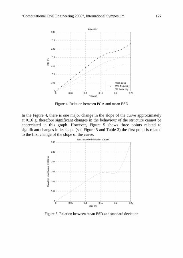
“Computational Civil Engineering 2008”, International Symposium 127
0 0.05 0.1 0.15 0.2 0.250
0.05
0.1
0.15
0.2
0.25
0.3
0.35
PGA (g)
ES
D (
m)
PGA-ESD
Mean curve
95% Reliability5% Reliability
Figure 4. Relation between PGA and mean ESD
In the Figure 4, there is one major change in the slope of the curve approximately at 0.16 g, therefore significant changes in the behaviour of the structure cannot be appreciated in this graph. However, Figure 5 shows three points related to significant changes in its shape (see Figure 5 and Table 3) the first point is related to the first change of the slope of the curve.
0 0.05 0.1 0.15 0.2 0.250
0.01
0.02
0.03
0.04
0.05
0.06
ESD (m)
Sta
ndar
d de
viat
ion
of E
SD
(m
)
ESD-Standard deviation of ESD
Figure 5. Relation between mean ESD and standard deviation

128 Y.F. Vargas, L.B. Pujades, A. H. Barbat, J.E. Hurtado
The second one is the first maximum and the third is related to the beginning of straight line with maximum slope, Later on, we use these points to discuss the behaviour of the structure. Table 3. Coordinates of the particular points in the figure 5 __________________________________________________ Point X coordinates Y coordinates ____ _____________ _____________ (m) (m) __________________________________________________ 1 0.13 0.0270 2 0.16 0.0294 3 0.23 0.0298 __________________________________________________
5. CAPACITY SPECTRUM, DAMAGE STATES AND FRAGILITY CURVES
5.1. Capacity Spectrum and bilinear representation
The capacity spectrum is the spectral acceleration-spectral displacement (Sa-Sd) representation of the capacity curve. Which is often used in its simplified bilinear form, defined by the yielding point (Dy,Ay) and the ultimate capacity point (Du,Au). Figure 6 shows a capacity spectrum of the RC building and its bilinear representation.
0.05 0.1 0.15 0.2 0.25 0.30
0.05
0.1
0.15
0.2
0.25
0.3
0.35
Spectral displacement (m)
Spe
ctra
l acc
eler
atio
n (g
)
Capacity spectrum and bilinear aproximation
Capacity spectrum
Bilinear aproximation
(Dy,Ay) (Du,Ay)
Figure 6. Capacity spectrum and bilinear representation

“Computational Civil Engineering 2008”, International Symposium 129
5.2. Damage states
In order to analyze expected damage we use simplified methods allowing to obtain damage states (Ds) thresholds and fragility curves. Four non-null damage states are considered: (1) slight, (2) moderate, (3) severe and (4) extensive-to-collapse. For a given damage state, the damage state threshold is defined by the 50% exceedance probability. This damage state threshold can be defined from the bilinear capacity spectrum, in a simplified way, as follows: (Lantada et al 2008).
.*7.01 DyDs (1.1)
.2 DyDs (1.2)
).(*25.0 2423 DsDsDsDs (1.3)
.4 DuDs (1.4)
This way, damage states thresholds have been calculated for all the obtained capacity spectra. Thus, being considered as random variables, Figure 7 shows all the results and the mean values of each damage state threshold. This figure shows how the dispersion increases with increasing damage states. This fact may indicate that when the structure enters into nonlinear behavior, the damage level has greater uncertainties.
0 0.05 0.1 0.15 0.2 0.25 0.30
0.05
0.1
0.15
0.2
0.25
0.3
0.35
Spectral Displacement (m)
Spe
ctra
l acc
eler
atio
n (g
)
Relation between Spectral acceleration and spectral displacement
Ds1
Ds2Ds3
Ds4
Figure 7. Damage states like random variables
The mean and standard deviation of Sa and Sd of each damage state, are shown in Table 4.

130 Y.F. Vargas, L.B. Pujades, A. H. Barbat, J.E. Hurtado
Table 4. M_________ ean and standard deviation of damage states _________________________________________
Ds Sd Sd Sa Sa
____ _ ___ __ ___ _____ 1 09 18 0.0038
___
s in Table 3 and Table 4. In for the damage states 2, 3
ponding fragility curve (FC), is defined by the in our case, the spectral displacement.
(m) (m) (g) (g) _________ _______ _______ _______ __
0. 85 0.0013 0. 78 2 0.1314 0.0017 0.2504 0.0050 3 0.1583 0.0049 0.1878 0.0051 4 0.2212 0.0148 0.2504 0.0054 _______________________________________________
It is important noting the agreement with the valueTable 3, points 1, 2 and 3 correspond to the mean values and 4.
5.3. Fragility curves
For each damage state, the corresprobability of being exceeded as a function,It is assumed that fragility curves follow a standard lognormal cumulative distribution function.
0 0.05 0.1 0.15 0.2 0.25 0.30
0.1
0.2
0.3
0.4
0.5
0.6
0.7
0.8
0.9
1Fragility Curves
Spectral displacement (m)
P[D
s/S
d]
FC1
FC2FC3
FC4
Figure 8. Example of the fragility curves for the building
Each fragility curve is then obtained from the equation 2:
SdLnSdDsP
1/
DsSdDs , (2)

“Computational Civil Engineering 2008”, International Symposium 131
Where:
is the spectral displacement. Sd
DsSd , is the mean value of the lognormal distribution, this is the corresponding state threshold as defined above. damage
Ds is the standard deviation of the natural logarithm of spectral displacement
of the Ds .
is the standard lognormal cumulative distribution function.
In ed d iations can be estimated by assuming that damage distribution follow a
bi ragility curves ob as the
quation (2) mean values can be determined from the capacity spectrum and standar ev
nomial distributions (See Lantada et al. 2008). Figure 9 shows the ftained for all the capacity spectra, obviously, according to Figure 7,
considered damage state increases the uncertainties involved in the corresponding fragility curve increases. See fragility curves corresponding to damage sates slight and collapse in Figure 9. Figure 10 shows the results of a sensitivity test on the influence of the mechanical properties of materials and the non-damage states thresholds. The stiffness is used as a variable in this test.
0 0.1 0.2 0.3 0.4 0.5 0.60
0.1
0.2
0.3
0.4
0.5
0.6
0.7
0.8
0.9
1Fragility Curves
Spectral displacement (m)
P[D
s/S
d]
FC1
FC2FC3
FC4
Figure 9. Fragility curves like random variables

132 Y.F. Vargas, L.B. Pujades, A. H. Barbat, J.E. Hurtado
7800 7900 8000 8100 8200 8300 84000
0.05
0.1
0.15
0.2
0.25
0.3
Stiffness (Kn/m)
Sd
(m)
Sensitivity analysis for the Ds
Ds1
Ds2Ds3
Ds4
Figure 10. Sensitivity analysis for the Ds
DS1 and DS2 damage states are practically independent of the stiffness, while for DS4 and DS3 the spectral displacement decreases with increasing stiffness indicating that the probability of the corresponding damage states increases with the stiffness.
0 0.1 0.2 0.3 0.4 0.5 0.60
0.1
0.2
0.3
0.4
0.5
0.6
0.7
0.8
0.9
1
Spectral displacement (m)
P[D
s/S
d]
Mean fragility Curves
FC1
FC2FC3
FC4
Figure 11. Mean fragility curves
Figure 11 shows the mean fragility curves, and Figure 12 shows the corresponding standard deviations as a function of Sd. This Figure clearly depicts the dependence of the uncertainties of the damage grades. For instance, the uncertainty of the
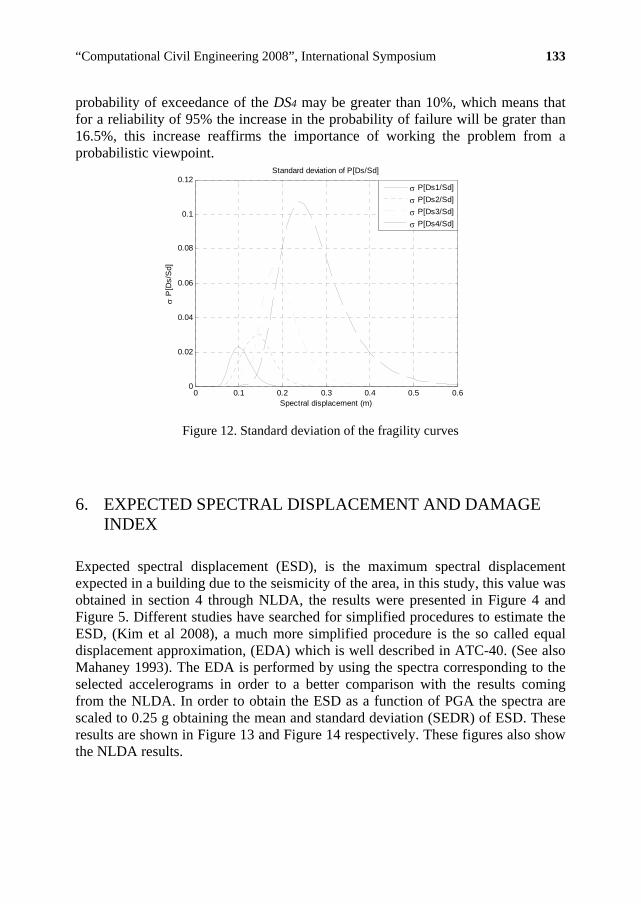
“Computational Civil Engineering 2008”, International Symposium 133
probability of exceedance of the DS4 may be greater than 10%, which means that for a reliability of 95% the increase in the probability of failure will be grater than 16.5%, this increase reaffirms the importance of working the problem from a probabilistic viewpoint.
0 0.1 0.2 0.3 0.4 0.5 0.60
0.02
0.04
0.06
0.08
0.1
0.12
Spectral displacement (m)
P
[Ds/
Sd]
Standard deviation of P[Ds/Sd]
P[Ds1/Sd]
P[Ds2/Sd]
P[Ds3/Sd]
P[Ds4/Sd]
Figure 12. Standard deviation of the fragility curves
6. EXPECTED SPECTRAL DISPLACEMENT AND DAMAGE INDEX
Expected spectral displacement (ESD), is the maximum spectral displacement expected in a building due to the seismicity of the area, in this study, this value was obtained in section 4 through NLDA, the results were presented in Figure 4 and Figure 5. Different studies have searched for simplified procedures to estimate the ESD, (Kim et al 2008), a much more simplified procedure is the so called equal displacement approximation, (EDA) which is well described in ATC-40. (See also Mahaney 1993). The EDA is performed by using the spectra corresponding to the selected accelerograms in order to a better comparison with the results coming from the NLDA. In order to obtain the ESD as a function of PGA the spectra are scaled to 0.25 g obtaining the mean and standard deviation (SEDR) of ESD. These results are shown in Figure 13 and Figure 14 respectively. These figures also show the NLDA results.
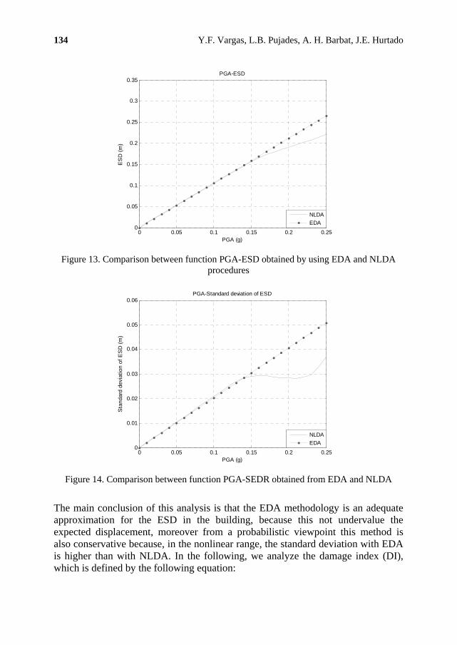
134 Y.F. Vargas, L.B. Pujades, A. H. Barbat, J.E. Hurtado
0 0.05 0.1 0.15 0.2 0.250
0.05
0.1
0.15
0.2
0.25
0.3
0.35
PGA (g)
ES
D (
m)
PGA-ESD
NLDA
EDA
Figure 13. Comparison between function PGA-ESD obtained by using EDA and NLDA
procedures
0 0.05 0.1 0.15 0.2 0.250
0.01
0.02
0.03
0.04
0.05
0.06
PGA (g)
Sta
ndar
d de
viat
ion
of E
SD
(m
)
PGA-Standard deviation of ESD
NLDA
EDA
Figure 14. Comparison between function PGA-SEDR obtained from EDA and NLDA
The main conclusion of this analysis is that the EDA methodology is an adequate approximation for the ESD in the building, because this not undervalue the expected displacement, moreover from a probabilistic viewpoint this method is also conservative because, in the nonlinear range, the standard deviation with EDA is higher than with NLDA. In the following, we analyze the damage index (DI), which is defined by the following equation:

“Computational Civil Engineering 2008”, International Symposium 135
)(4
1 4
0i
i
DSiPDI
(3)
P(DSi) is the probability of the damage state i and can be easily calculated from fragility curves. Figure 15 shows this procedure for calculating these probabilities. DI can be understood as the normalized mean damage grade and it is a measure of overall damage in the structure. DI can be also plotted as a function of ESD. Thus, the DI can be calculated for any spectral displacement but the comparison of DI obtained with EDA and NLDA, requires computing the PGA corresponding to each ESD.
0 0.05 0.1 0.15 0.2 0.250
0.1
0.2
0.3
0.4
0.5
0.6
0.7
0.8
0.9
1
ESD
PD
s/S
d
Probability of each damage state
P Null
P Slight
P Moderate
P Extensive
P Complete
Figure 15. Probability of each damage state depending ESD
Figure 16 shows the obtained results: Namely, mean values and 95% reliability curves.
Again, our results confirm that the EDA is conservative respect to NLDA, even when considering a reliability of 95% for random variables, but, if the variables were no treated from a probabilistic approach, this would result in an underestimation of the actual damage that may occur in the building. In the case of the building analyzed in this work, the damage index estimated by using a deterministic approach could be 0.25 lesser than the one computed from a probabilistic viewpoint.

136 Y.F. Vargas, L.B. Pujades, A. H. Barbat, J.E. Hurtado
0 0.05 0.1 0.15 0.2 0.25 0.3 0.35 0.40
0.1
0.2
0.3
0.4
0.5
0.6
0.7
0.8
0.9
1
PGA
DI
Damage Index obtained with EDA and NLDA
NLDA
EDANLDA 95% Reliability
EDA 95% Reliability
Figure 16. Damage index obtained with NLDA, EDA, and reliability of 95%
7. DISCUSION AND CONCLUSIONS
This paper contains the assessment of the vulnerability fragility and expected damage in a reinforced concrete building. However, the results here obtained go further and they concern to the comparison of nonlinear static and dynamic analysis procedures. Here, we use both types of analysis for the calculations. Furthermore, we face the problem from a probabilistic point of view, since the parameters related to the mechanical properties of the materials and the seismic demands are considered as random variables. A first hint is that notwithstanding that NLDA is a powerful tool in the assessment of the structural behaviour of buildings when submitted to seismic actions, this procedure has little or no sense if the seismic demand is not carefully and properly selected. We put special care in the selection of the accelerograms used in this study. We have selected accelerograms corresponding to seismic events from the Spanish and European strong motion records databases. In order to observe a wide range of spectral displacements the Eurocode type 1 design spectrum for soils type D has been taken as target demand spectrum. The accelerograms have been selected according to this criterion and have been scales to cover PGA values until 0.25 g. We use standard pushover analysis to obtain probabilistic capacity curves. A modified adaptive technique has been used to define the horizontal incremental load limit to automatically stop the pushover analysis in a great number of massive runs.

“Computational Civil Engineering 2008”, International Symposium 137
Starting from capacity spectra, simplified methods allow obtaining damage states thresholds and probabilistic fragility curves. An interesting conclusion of this exercise is that uncertainties increase in the nonlinear range. For the collapse damage state, the uncertainties in the fragility curves may be greater than 10%. EDA and NLDA are used to obtain the expected spectral displacement ESD and their standard deviations as a function of the PGA. Again, uncertainties increase with increasing PGA. This fact can be attributed to the increase of the inelastic behaviour of the building. EDA is a successful approach because does not underestimate the actual displacement, but in structures with higher ductility can be much conservative. Furthermore, the fact that both ESD and SEDR are greater in EDA than in NLDA confirms that EDA is conservative. In the NLDA, the seismic action is the main responsible for uncertainties in the spectral response, being less significant the influence of the uncertainties in the mechanical properties of the building. However, as the damage state increases a sensitivity test shows a correlation between stiffness and spectral displacement. For damage states DS3 and DS4 the spectral displacement decreases with increasing stiffness indicating that the probability of the corresponding damage state increases with the stiffness. This result is important since the damage states 3 and 4 have a high influence in the calculation of the damage index. Finally, the comparison of the damage index as a function of PGA and the corresponding uncertainties shows that, for damage states from severe to collapse and for a reliability of 95%, the uncertainties in the damage index may be higher than 0.25 units or 42% of the damage index. Thus, perhaps the most important conclusion is that, both static and dynamic structural analyses should be faced by using probabilistic approaches.
References
1. ATC-40. 1996. Seismic evaluation and retrofit of concrete buildings, Applied Technology Council, Redwood City, California
2. Borzi B, Phino R, H. Crowley 2007. Simplified Pushover analysis for large-scale assessment of RC buildings. Engineering Structures 30 (2008) 804-820.
3. Eurocode 8. 2004. Design of structures for earthquake resistance. Part 1: General rules, seismic actions and rules for building
4. Kim S.P & Y.C. Kuruma 2008. An alternative pushover analysis procedure to estimate seismic displacement demands. Engineering structures 30 (2008) 3793-3807.
5. Lantada N, Pujades LG & AH. Barbat. Vulnerability index and capacity spectrum based methods for urban seismic risk evaluation. A comparison. Natural Hazards 51:501-524
6. MATLAB. The mathworks inc. 7. Mwafy A.M & Elnashai. A.S 2001. Static pushover versus dynamic collapse analysis of RC
buildings. Engineering Structures 23 (2001) 407–424. 8. Poursha M, Khoshnoudian F & AS. Moghadam. 2009. A consecutive modal pushover procedure
for estimating the seismic demands of tall buildings. Engineering Structures 31 (2009) 591-599 9. Vamvatsikos D and CA. Cornell 2002. The Incremental Dynamic Analysis and its application to
Performance-Based Earthquake Engineering. Proceeding of the 12th European Conference on Earthquake Engineering, London September 2002

“Computational Civil Engineering 2010”, International Symposium Iasi, Romania, May 28, 2010
Paving Blocks Compressive Strength Evaluation by Impact Hammer
Jiri Brozovsky1, David Prochazka2, Dalibor Benes3
1,2,3 Institute of Building Materials and Components , Faculty of Civil Engineering, Brno University
of Technology, 602 00Brno, Czech Republic
Summary
The quality control of building material is prerequisite of its quality attainment and maintenance. These problems are continually actual in the face of competitive environment in the building material industry and ever-growing demand of consumers. Also the fact that many manufacturers have established (or are establishing) their Quality Management System in accordance with the CSN EN ISO 9000 Standard series, plays an important role. One of integral parts of this QM System is also implementation of the product interoperable quality control. One of possibilities of paving blocks operative strength evaluation is application of nondestructive test methods. This paper describes calibration correlations for paving blocks compression strength determination using both Schmidt impact hammer type N and L. Calibration correlations determined vary between 0.91 and 0.87 which means that these calibration correlations are implementation able in practice.
KEYWORDS: concrete, strength, rebound number, impact hammer, paving block.
1. INTRODUCTION
The quality control of building material is prerequisite of its quality attainment and maintenance. These problems are continually actual in the face of competitive environment in the building material industry and ever-growing demand of consumers. Also the fact that many manufacturers have established (or are establishing) their Quality Management System in accordance with the CSN EN ISO 9000 Standard series, plays an important role. One of integral parts of this QM System is also implementation of the product interoperable quality control. Taking into consideration that these companies do not keep their own test rooms, such interoperable quality control does limit itself only to product appearance/size monitoring. Strength characteristics are monitored to limited extent namely with check tests in outside test rooms because of lack of in–house test rooms, as mentioned above.

“Computational Civil Engineering 2010”, International Symposium 139
Some products with critical compression strength are pressed and vibropressed concrete wares. This property is checked - as well as on concrete - at the age of 28 days. Eventual strength non-conformities are detected mainly after product handover to customers and, what is worse, generally after building into construction. That is why operative production alterations are limited.
One of possibilities of pressed/vibropressed products operative strength evaluation is application of nondestructive test methods. These concrete nondestructive test methods enable prompt parameter evaluation of nondestructive testing. Acquisition costs of appropriate instrumentation are far fewer than the costs of destructive ones (loading jacks); they do not require special rooms for test instrumentation location. Existing applications of test methodology and calibration relations as codified in current concrete test standards are questionable since calibration relations relate to concrete over 14 days; test cube edges are 150 mm in length, and maximum grain size is not inconsiderable as well.
This paper describes calibration correlations for paving blocks compression strength determination using both Schmidt impact hammer type N and L.
2. TESTING PROCEDURES
2.1 Schmidt test hammer
The tests were performed by Schmidt hammer type N and L, having the following characteristics:
Schmidt test hammer type N: impact energy 2.207 N.m, compressive strength characteristics of concrete with the range of 10 to 70 MPa.
Schmidt test hammer type L: impact energy 0.735N.m, compressive strength characteristics of concrete with the range of 10 to 70 MPa.
2.1 Postup při zkoušení a vyhodnocení výsledků zkoušek
Testing stand providing fixed gripping by pressure steel plates guided by vertical guide bars. Grip force: 14 to 15 N.m by means of torque wrench. See the Fig. 1 for test samples gripping.
Zkušební plocha : byla za sucha obroušena diamantovým brusným kotoučem, aby bylo dosaženo rovného hladkého povrchu a byla viditelná zrna kameniva; nedestruktivní zkoušky byly prováděny na spodní ploše zámkové dlažby.

140 J.Brozovsky and D. Prochazka.
Figure 1. Test sample gripping during non-destructive tests
Zkoušení: minimum distance between individual testing spots and/or paving block edge: 25 mm. Bottom horizontal surface is being tested (paving blocks are manufactured in two layers as a rule i.e. top concrete wear layer quality differs from the concrete core of its own). Minimum readings: 8.
Vyhodnocení výsedků zkoušek : test ends in a set of rebound numbers. A set of particular rebound Rzi values serves to calculation of mean rebound number Rz and maximum/minimum limits deviating 13 % from mean rebound number. Rebiund number Rz out of these limits are rejected. Remaining valid measurements shall serve for mean calculation once more, being assigned with corresponding compressive strength value of fPBL of unconfirmed accuracy using appropriate calibration correlation. In case less than 6 valid values remains (after rejecting extreme Rzi values, the product under testing is to be suspended and replaced by a new ones).
2.2 Postup při zkoušení a vyhodnocení výsledků zkoušek
Paving blocks are tested for compression strength in a press using pressure steel plates thick 30 mm at the least.
These plates are sized in line with block thickness, observing CSN 73 6131-1. For instance – blocks 60 mm thick shall use 60 x 120 mm pressure steel plates and for pavement thickness of 80 mm plates dimension of 80 x 120 mm –see figure2.

“Computational Civil Engineering 2010”, International Symposium 141
Figure 2. Paving block compressive strength test according to CSN 73 6131-1
Block pressure surface planing: grinding of both surfaces i.e. wear layer and bottom surface.
Compression strength is calculated using formula (1) as follows:
c
b A
FR [MPa] (1)
where:
Rb – compression strength F – destruction force in N Ac – pressure surface in mm2

142 J.Brozovsky and D. Prochazka.
3. TEST RESULTS AND CALIBRATION CORRELATIONS
3.1 Test results
There are listed testing results of 315 rectangular paving blocks sized 200 × 100 × 60 mm, made in the manufacturing plants. These blocks were tested at age of 3, 7, 14, 21, and 28 days.
Based on both destructive and non-destructive test results, calibration correlations have been elaborated using method of least squares to determine compression strength following rebound number.
Výsledky zkoušek jsou znázorněny v obrázku 3 (Schmidt test hammer type N) a v obrázku 4 (Schmidt test hammer type L)
y = 0,04x2 - 0,2558x + 20,134
30
40
50
60
70
80
90
22 26 30 34 38 42 46
Rebound number [-]
Com
pre
ssio
n s
tren
gth
[M
Pa]
Figure 3. Paving block compression strength test results using Schmidt impact hammer type N

“Computational Civil Engineering 2010”, International Symposium 143
y = 0,023x2 + 0,7235x + 10,62
30
40
50
60
70
80
90
100
110
18 22 26 30 34 38 42 46 50
Rebound number [-]
Com
pre
ssio
n s
tren
gth
[M
Pa]
Figure 4. Paving block compression strength test results using Schmidt impact hammer
type L
3.2 Calibration correlation
For calibration correlation – as expressed by straight line dependence – are correlation closeness and, subsequently, its efficiency in practice evaluated in terms of r correlation coefficient value. This one defines correlation closeness between compression strength and non-destructive testing parameter. See [1] for correlation coefficient relevance as follows:
0.7 r 0.9 - High degree of correlation closeness
r 0.9 - High cohesion between variables
144 J.Brozovsky and D. Prochazka.
In point of practical utilization, calibration correlation corresponding to correlation coefficient r 0.85 is acceptable.
Below are described calibration correlations as elaborated for particular typy tvrdoměrů:
Schmidt test hammer type N 1.202558.004.0 2 NNNpbl RRf r=0,911 (2)
Schmidt test hammer type N 6.107235.0023.0 2 LLLpbl RRf r=0,868 (3)
4. CONCLUSIONS
Based on experimental testing results, calibration relations have been elaborated to determine paving block compression strength using hammer rebound number; For Schmidt hammer type N the calibration relation shows high cohesion between variables, correlation coefficient r = 0,911. For calibration relation elaborated for Schmidt hammer type L the correlation coefficient is 0,868 – this shows high cohesion of correlation nevertheless, such value is bound to practical usability.
Impact hammer testing methods are based on hardness of concrete cement binder. In case of paving blocks, the maximum nominal aggregate gradation is lower than the same in structural concrete (up to 8 mm as a rule); however, space between coarse aggregates is smaller creating more compact structure. That is why – using Schmidt impact hammer – these aggregates are affected to a certain extent, even if the test spots are chosen as carefully as possible.
Schmidt impact hammer type L rebound number at one test spot shows greater diffusion than the same in case of hammer type N, which is explainable through better response of the hammer type L to macrostructure of concrete under testing. As stated above, the Schmidt impact hammer type L is inadvisable.
Acknowledgements
The work was supported by the MSM 0021630511 plan: Progressive Building Materials with Utilization of Secondary Raw Materials.

“Computational Civil Engineering 2010”, International Symposium 145
References
1. Drochytka R. et al. Progressive Building Materials with Utilization of Secondary Raw Materials and their Impact on Structures Durability. but, Final report of the project VVZ CEZ MSM: 0021630511, Brno 2008. Brozovsky J.: Subtask 3 (in Czech).
2. Brožovský, J. Matějka, O. Martinec, P. Concrete Interlocking Paving Blocks Compression strenght Determination Using Non-Destructive Methods. The e-Journal of Nondestructive Testing, 2007, roč. 12, č. 4, s. 91-97. ISSN: 1435-4934.
3. Brožovský, J., Fojtík, T. , Brožovský, J., jr. Built-in Concretes Made with Gypsum Free Cements: Compression Strength Determination Using Nondestructive Testing Methods. In The Third International Conference on Structural Engineering, Mechanics and Computation, Cape Town, South Africa, 2007, ed. A. Zingoni, Millpress Science Publishers, Rotterdam The Netherlands, p. 1554-1559, ISBN 978 90 5966 057 1
4. Brožovský, J., Zach, J. , Brožovský, J., jr. Gypsum free cements and concretes made with them: strength determination using nondestructive testing methods. In IV Conferencia Panamericana for Non destructive Testing, Buenos Aires, Argentina, 2007, Primera edición, Asociación Argentina de Ensayos No Destructivos y Estructurales, p. 1-9, (paper №2), ISBN 978-987-23957-0-4
5. EN 12504-2: Testing of Concrete in Structures – Part 2: Non-Destructive Testing - Determination of Rebound Number
6. CSN 73 1370: Non-Destructive Testing of Concrete: Common Regulation. 7. CSN 73 1373: Testing of Concrete by Hardness Testing Methods. 8. ISO/DIS 8045: Concrete, hardened -Determination of rebound number 9. ASTM C 805-97: Standard Test Method for Rebound Number of Hardened Concrete 10. BS 1881, part 202: Testing concrete. Recommendations for surface hardness testing by
rebound hammer 11. NFP 18-417: Bétons – Mesure de la dureté de surface au sclérométre 12. JGJ/ T 23-2001: Technical Specification for Inspection of Concrete Compressive Strength
by Rebound Method

“Computational Civil Engineering 2010”, International Symposium Iasi, Romania, May 28, 2010
Concrete durability with addition of fluidized ash in sulphate and chloride aggressive environment
Jiri Brozovsky1, David Prochazka2
1,2 Institute of Building Materials and Components , Faculty of Civil Engineering, Brno University
of Technology, 602 00Brno, Czech Republic
Summary
The article presents durability monitoring results of concrete with the addition of fluidized ash exposed to aggressive media, concretely in water containing chlorides and sulphates. In the concrete a part of small aggregate was replaced by fluidized bed ash from black coal combustion power plant in Trinec. Small aggregates were replaced by a quantity of 0 – 50 %. Samples of concrete were placed in given environments for 24 months.
KEYWORDS: Concrete, fluidized ash, fluid ash, durability, sulphates, chlorides
1. INTRODUCTION
Industrial ashes exploitation for building material production continues permanently in the course of many years. One of wastes exploitable with concrete production is also fluidized ash. To use these ash concretes in practice there is necessary to know not only their basic physical–mechanical characteristics but also other properties, among others their resistance to aggressive media. Our research works have been focused on monitoring of concrete chloride/sulphate resistance after addition of deposit fluid combustion ash.
2. THE FLUID ASHS CHARACTERISTIC
Fluidized ashes originate in the course of flue gases desulphurization based on direct mixing of fuel with desulphurising reagent (generally lime or dolomite in some cases) before combustion or during it. There are many production processes; most of them are patent covered. Generally all these processes are based on calcinations of present desulphurising reagent to CaO and its subsequent reaction with sculpture oxides along with oxidation of sulfur dioxide to sculpture trioxide.

“Computational Civil Engineering 2010”, International Symposium 147
This reaction results in mixture of original fuel ash, unreacted desulphurising reagent (CaO with CaCO3 remains, as the case may be), calcium sulfate, ash matter product reaction with CaO, and unburned fuel. Since fluid combustion temperatures are lower than classic combustion ones, unreacted CaO is present in the form of so called burned lime, therefore reactive lime. Fluid ashes are also typical for their low volume of melt.
That is why each fluid combustion unit products in principle fluid ashes of two kinds: furnace space ash (called fluidized bed ash), and light ash (called fluidized fly ash). Characteristics of both these ashes are different as to physical properties (granulometry, specific surface, density, powder density) as well as chemical and mineralogical composition even if they originate from identical fluid combustion and desulphurization technologic procedure. Both types of ash have variable characteristics due to combustion process instability and variability of input component properties (coal and desulphurising reagent).
3. PARAMETERS OF RAW MATERIALS AND CONCRETE COMPOSITION
For the production of concrete were used such materials: binder – cement CEM I 42,5 from the Mokrá cement factory; aggregates – fine – extracted from the locality Bratčice, fraction 0/4 mm, –
coarse – crushed from the locality Olbramovice, fraction 4/8, 8/16 mm; ash – fluidized bed from the black coal combustion Třinecké železárny
Třinec – results of chemical and phase composition are shown in Table 1.
Table 1. Třinec fluidized bed ash chemical/ phase composition A. Chemical composition
Tested components
Component share [%]
Tested components
Component share [%]
SiO2 53.5 MnO 0.1 Al2O3 21.5 K2O 2.6 Fe2O3 5.8 Na2O 0.2 TiO2 0.9 S 2.5 CaO 6.7 C 2.6 MgO 3.2 Annealing loss 0.46
B. Phase composition Ash contains considerable volume of –silica. Only small volume of anhydride has been detected. That is why there is possible to assume low share of partly decomposed potassic feldspar (orthoclase) and lesser share of illite and hematite.

148 J.Brozovsky, D. Prochazka.
Testing of concrete with deposit fluid ash as partial replacement of fine aggregates has been carried out using 3 kind of concrete with variable ash content and ashless concrete mixture as reference test sample. See the Table No. 2 for composition of particular concrete mixtures.
Table 2: Concrete mixture composition for experimental works Concrete mixture composition per
1m3 C0A C20A C30A C50A
CEM I 42.5 R cement 330 330 330 330 Sand 0 to 4 mm from the Bratčice Gravel Pit
756 605 529 378
Ash from the Chvaletice Power Plant
0 151 227 378
Aggregates 8 to16 mm from the Olbramovice Gravel Pit
1069 1069 1069 1069
Water 199 199 199 199
4. TEST METHODOLOGY
To investigate concrete resistance to corrosion there were prepared test specimens (blocks 40 × 40 × 160 mm each) conformable to the ČSN 73 1340 Standard.
After manufacturing the test specimens have been placed into moist environment for 24 hours followed - after form removal and before exposition to corrosive medium - by placing into water bath at 19 to 21°C. After 28 hour hardening the specimens have been exposed to corrosive medium action. Selection of parameters under evaluation is based on the ČSN 73 1340 Standard.
Tested specimens will be monitored in light of parameters as follows: appearance (visually) density of hardened concrete (EN 12390-7 ) ultrasonic pulse velocity (EN 12504-4) and dynamic modulus of elasticity
Ebu (CSN 731371) compressive and flexural strength strength fcc (EN 1015-11)
Specimen strength has been destructive tested before exposition to corrosive medium and after 3, 9, 15, 18, and 24 months of exposition.
Corrosive environment effect during other time periods has been evaluated based on both ultrasonic pulse speed variation and dynamic moduluses of elasticity.
Corrosive media: sulphates - sodium sulphate solution (10,000 mg of SO4
2- in 1 litre) and chlorides - 5 % solution of NaCl .

“Computational Civil Engineering 2010”, International Symposium 149
5. CONCRETE DURABILITY TEST RESULTS
The test results are shown in Figure 1 to 6; figure 1 to 3 – changes in the strength and dynamic modulus, depending on the time of exposure of concrete in sulphate environments.
5
5,5
6
6,5
7
7,5
88,5
9
9,5
10
0 3 6 9 12 15 18 21 24
Expositoon period [months]
Fle
xura
l str
engt
h [M
Pa]
C0 C20A C30A C50A
Figure 1. Changes in flexural strength during concrete exposure in sulphates for 24 months
40
45
50
55
60
65
70
0 3 6 9 12 15 18 21 24
Expositoon period [months]
Com
pres
sive
str
engt
h [M
Pa]
C0 C20A C30A C50A
Figure 2. Changes in compressive strength during concrete exposure in sulphates for 24 months

150 J.Brozovsky, D. Prochazka.
38
42
46
50
0 3 6 9 12 15 18 21 24
Expositoon period [months]
Dyn
amic
mod
ulus
of
elas
tici
ty [
GP
a]
C0 C20A C30A C50A
Figure 3. Changes in dynamic modulus of elasticity during concrete exposure in sulphates for 24 months
5
5,5
6
6,5
7
7,5
8
8,5
9
0 3 6 9 12 15 18 21 24
Expositoon period [months]
Fle
xura
l str
engt
h [M
Pa]
C0 C20A C30A C50A
Figure 4. Changes in flexural strength during concrete exposure in chlorides for 24 months

“Computational Civil Engineering 2010”, International Symposium 151
40
45
50
55
60
65
70
0 3 6 9 12 15 18 21 24
Expositoon period [months]
Com
pres
sive
str
engt
h [M
Pa]
C0 C20A C30A C50A
Figure 5. Changes in compressive strength during concrete exposure in chlorides for 24 months
38
42
46
50
0 3 6 9 12 15 18 21 24
Expositoon period [months]
Dyn
amic
mod
ulus
of
elas
tici
ty [
GP
a]
C0 C20A C30A C50A
Figure 6. Changes in dynamic modulus of elasticity during concrete exposure in chlorides for 24 months

152 J.Brozovsky, D. Prochazka.
6. CONCLUSIONS
To evaluate concrete resistance to aggressive medium (chlorides in this instance - 12 months evaluation time period according to the ČSN 73 1340 Standard) there is necessary to ensure that no one parameter under monitoring shall decrease during this interval.
a) Resistance to Sulphates
There is possible to treat tested concrete with 50 % of fluid combustion ash (replacement of fine natural aggregates) as resistant to sulphates.
Other tested concretes including reference ashless concrete are unfit to stand up to sulphates by reason of monitored parameter deterioration before expiration of 12 months exposition (6 to 9 months). Concrete with 50 % of deposit fluid ash shown highest resistance; on the other hand concrete where 20 % of fine aggregates have been replaced with fluid combustion ash shown least resistance.
b) Resistance to Chlorides
Based on monitoring results as mentioned above there is possible to state that tested concretes with 50 % of fluid combustion ashes (place of origin: TŽ Třinec Co.) as replacement of natural aggregates are resistant to chlorides.
Other tested concretes including reference ashless concrete are unfit to stand up to chlorides by reason of monitored parameter deterioration before expiration of 12 months exposition (6 to 9 months). Concrete with 50 % of deposit fluid ash shown highest resistance; on the other hand concrete where 20 % of fine aggregates have been replaced with fluid combustion ash shown least resistance.
Tests have shown that partial substitution of small aggregates with fluid bed ash can increase concretes resistance to chlorides and sulphates. To achieve the desired durability of concrete, 40 to 50 % of small aggregates can be replaced by fluid bed ash.
Acknowledgements
The work was supported by the MSM 0021630511 plan: Progressive Building Materials with Utilization of Secondary Raw Materials.

“Computational Civil Engineering 2010”, International Symposium 153
References
1. Drochytka R.: et al. Progressive Building Materials with Utilization of Secondary Raw Materials and their Impact on Structures Durability. but, Final report of the project VVZ CEZ MSM: 0021630511, Brno 2008. Brozovsky J.: Subtask 3 (in Czech).
2. Brožovský, J., Bydžovský, J., Brožovský, J. Влияние состава заполнителя и толщины цементного теста на расход цемента в бетонах на безгипсовом портландцементе. Научно-технический и производственный журнал Бетон и железобетон в Украине, №4(50) 2009, str.7-10
3. Brožovský, J., Zach, J. El uso de elementos de despolvoreamiento originados del tratamiento de áridos utilizados para la fabricación del cemento In : XIV Convención científica de ingeniería y arquitectura (CCIA 14),Habana, Cuba ed. Ministerio de educación Superior, La Habana, Cuba, 2008, str. 360-367, ISBN 978-959-261-281-
4. Brožovský, J. Стойкость цементов со сталеплавительным шлаком против агрессивного CO2. In VII – я Международная научно-практическая Интернет – конференция „СОСТОЯНИЕ СОВРЕМЕННОЙ СТРОИТЕЛЬНОЙ НАУКИ – 2009», ed. Сб. науч. Трудов – Полтава : Полтавский ЦНТЭИ a časopis Бетон и железобетон в Украине, Poltava, Ukraine, 2009, pp. 1-5
5. Brožovský, J., Fojtík, T., Dufka, A. Resistance of Concrete with Fine-Ground Granulated Slag Admixture to Sulphates and Acidic Aggressive Media. . INTRESECTIONS, ed. "Matei - Teiu Botez", Academic Society, 2007, vol. 4, No 4, p. 89-98, ISSN 1582-3024
“Computational Civil Engineering 2010”, International Symposium Iasi, Romania, May 28, 2010
Computational simulation for concrete slab with spherical gaps
Sergiu Călin1, Mugurel Cloşcă2, Gabriela Dascălu3, Ciprian Asăvoaie4 1Department of Concrete Structures, Building Materials, Technology and Management, “Gh. Asachi”
Technical University of Iasi, Faculty of Civil Engineering and Building Services, Iasi, 700050, Romania, e-mail: [email protected]
2Department of Concrete Structures, Building Materials, Technology and Management, “Gh. Asachi” Technical University of Iasi, Faculty of Civil Engineering and Building Services, Iasi, 700050,
Romania 3Department of Concrete Structures, Building Materials, Technology and Management, “Gh. Asachi”
Technical University of Iasi, Faculty of Civil Engineering and Building Services, Iasi, 700050, Romania
4Department of Concrete Structures, Building Materials, Technology and Management, “Gh. Asachi” Technical University of Iasi, Faculty of Civil Engineering and Building Services, Iasi, 700050,
Romania
Summary
Because there has been a lot of a discussion about the technical and economic advantages of the floor slabs and studied system is part of the field a plus of information is brought by detailing of some specific computational methods. The study will be detailed with each stage and by specifying the working steps in defines the structures in computational computer designing programs.
Among the known ones, under the circumstances of lack of the specific norms and under the time pressure, the designers used approximate methods in determining of the efforts, overestimated, own to the similar classical systems, which behavior under the loads differs to some extent.
This must be eradicated as soon as possible from the current practice, to avoid compromising these structural systems, fact happened with other valuable ideas in the civil engineering field. In this article it is detailed an original method of calculation, particularly useful in designing of the concrete slab with spherical gaps.
KEYWORDS: equivalence area, slab meshing, displacement, state of efforts and tensions.
1. INTRODUCTION
We state that local specialists (engineers and architects) who prefer their use assumes a clear responsibility, because in our country there is only informative prescription calculation and composition of such constructive systems and would require a Romanian standards based motivation [1].

“Computational Civil Engineering 2010”, International Symposium 155
There have been performed three different tests in the calculation methodology used; the analysis is made on a BD280 type ministructure with floor openings with 5x5m between elements bearings.
The aim of this study is to refine aspects regarding concrete slab with spherical gaps in order to achieve a rational reinforcement of all elements making up the floor. In Table 1 there are detailed characteristics of the concrete slab with spherical gaps, in accordance with Romanian technical approval from [2].
Table 1. Concrete slab with spherical gaps characteristics
Thickness of the slab
Sphere diameter
Own weight Slab elements
Concrete use în situ
Floor opening Type of
slab
[mm] [mm] [daN/m2] [m3/m2] [m]
BD 230 230 Ø 180 370 0,10 7-10 BD 280 280 Ø 225 460 0,14 8-12 BD 340 340 Ø 270 550 0,18 9-14 BD 390 390 Ø 315 640 0,20 10-16 BD 450 450 Ø 360 730 0,25 11-18
OBS: Own weight of the BubbleDeck slab element with gaps (BD) is function of the gaps dimensions. Maximum dimension for floor elements: Width: 3m Length: 9-14m (depending of the producer)
2. MODELLING PRESENTATION
Component elements of concrete slab with spherical gaps are slabs with ribs on two fronts, made of reinforced concrete or prestressed concrete. For these slab elements, the concrete link between the base and top, is performed by means of vertical ribs, formed around the spherical gaps [4], [5], [6].
The gaps in concrete are achieved by inclusion of high density polypropylene spheres, arranged in accordance with the design and fitting mounted between the nets. The distance between holes is 1/9 of their diameter [2], [3].

156 S. Călin, M. Cloşcă, G. Dascălu, C. Asăvoaie
Polypropylene spheres gaps Top reinforcement
Bottom reinforcement
Vertical ribs
Figure 1. Component elements of concrete slab with spherical gaps
Introducing spherical gaps in the floor leads to the adoption of a specific methodology of calculation, in our country so far there are no calculation rules to for such structural constructive systems [8].
2.1. Version I
In a first phase, in consultation with foreign experts, regarding the designing of concrete slab with spherical gaps it was recommended that we consider it as a compact floor [6], [9].
Later they started to introduce in the program the numerical modeling of a compact slab floor thickness of 28 cm.
Figure 2. Introducing data in the designing program for Version I
Figure 3. Slab meshing Figure 4. Deformed structure

“Computational Civil Engineering 2010”, International Symposium 157
It was made the meshing in the finite element and then the calculation of the structure with the results of the structure diagrams and maps of tensions that are shown in Figures 3, 4 and 5.
Figure 5. Slab tension for the slab
2.2. Version II
In the first version there were no difficulties encountered in placing the structure in the calculation program instead it was desired an analysis that takes into account the gaps that exist in the floor. To simplify the calculation it was made an equivalence between computing and the actual section. The equivalence is shown schematically in Figure 6.
Because of the boundaries of the spheres, the section of the ribs has a particular shape that leads to a number of difficulties in introducing the data into the program [10]. Equivalence was achieved through assimilating the spherical shaped gaps with a hollow cube. By adopting this solution resulted in the ribs a double T-shaped section.
Figure 6. The equivalence of the sections of the concrete slab with spherical gaps
After determining the shape of the rib section and calculating the equivalent areas we started introduction the input data to the computer program, closed bidirectional cased floor being the chosen model, shown in Figure 7.

158 S. Călin, M. Cloşcă, G. Dascălu, C. Asăvoaie
Figure 7. Introduction the input data to the computer program for Version II
Similar to the version I loads have been added to the floor and there have been performed the analyze that gave the efforts and stress states and the behavior of the floor, Figures 8 and 9.
Figure 8. Tensions maps of the slab Figure 9. The structural deformation
2.3. Version III
Because the previous versions do not allow a precise analysis for sizing and fitting all the elements of this type of floor, was made an original method of calculation developed by the team from BMTO Department Faculty of Engineering and Installation of Iasi, especially useful in designing the concrete slab with spherical gaps system [7].
It was made the equivalence of the vertical ribs with small beams with section as shown in Figure 10 [11]. These small beams were ordered on two orthogonal directions, forming a network of beams, which, as will be seen from the calculations, working particularly advantageous in the taking over the efforts, Figure 11. It will be displayed; both at the bottom and at the upper part a plate having a thickness resulting from the calculation, the sizes and the dimensions are varying depending on the thickness used floor. In the bearing plate on pillars, are

“Computational Civil Engineering 2010”, International Symposium 159
arranged the column heads embedded in the plate, in that area there are no gaps, Figures 12 and 13.
Figure 10. The equivalence of the sections Figure 11. Small beams intersection detail
Figure 12. Introduction the input data to the computer program for Version III
Loads were placed on the slab, and after performing the static calculations resulted efforts diagrams for each rib and efforts maps for the upper and lower slab and how the elements are deformed, Figures 14 and 15.
Figure 13. The experimental model in the Figure 14. Structural deformation
calculation program
Figure 15. The obtained results

160 S. Călin, M. Cloşcă, G. Dascălu, C. Asăvoaie
In this version of calculation it becomes easy to see areas of concentration of efforts and rational reinforcement can be achieved for all the elements of the slab, ribs, plates and column heads.
3. CONCLUSIONS
This designing system was introduced in practice in many daily use, based on thorough research, which fully proved the correctness of using it [12].
It has been aimed to meet specialist who want to use this relatively new system design by detailing specific methods of calculation. Studies and the methodologies detailed in this article reveal the behavior under load action and accurate results and encourage and justify their implementation in practice in our country and beyond. However, careful examination of its tools has to be done in order to choose the optimum modeling strategy.
It is considered that the study of the concrete slab with spherical gaps, improving the calculation methods, test methods and their standardization are important goals for future research.
Annex
Concrete slab with spherical gaps in images:
Figure 16. Aspects during casting in place of the concrete slab with spherical gaps
Figure 17. Parking places made with concrete slab with spherical gaps system

“Computational Civil Engineering 2010”, International Symposium 161
Figure 18. Constructions made with concrete slab with spherical gaps system
References
1. EN 1992-1-1:2004 Eurocode 2: Design of Concrete Structures. 2. Agrement Tehnic 007-01/120-2007 - BubbleDeck. (in Romanian) 3. Standard Român SR EN 13747:2006 “Produse prefabricate de beton – Predale pentru sisteme de
planşee”. (in Romanian) 4. Agrément certification KOMO Technical Certificate, 2006. 5. Lighter Flat Slab Structures with BubbleDeck – Part 1, February, 2006. 6. Design Guide from BubbleDeck United Kingdom – The Biaxial Hollow Deck – The way to new
solutions. 7. Mihai P. – „Proiectarea construcţiilor din beton armat” Ed. Societăţii Academice Matei-Teiu
Botez, Iaşi, 2009. (in Romanian) 8. Zoltán K., Oneţ T. – „Proiectarea structurilor de beton după SR EN 1992-1”, Ed. Abel, Cluj
Napoca, 2008. (in Romanian) 9. Von Emilie Veillon, UEFA-Verwaltungsgebäude in Nyon Eine runde Sache, Nr. 4, Freitag, 29.
Januar 2010. 10. Robot Millennium v.20.1. Autodesk Inc, 2008. 11. Axis VM9.0 Visual Modeling for Structural Analysis. 12. www.bubbledeck.com.

“Computational Civil Engineering 2010”, International Symposium Iasi, Romania, May 28, 2010
Environmental impact analysis of artificial aggregate burning process
Vít Černý 1, Rostislav Drochytka 2, Karel Kulísek 3 1 Faculty of Civil Engineering, Brno University of Technology, Brno, 662 37, Czech Republic 2 Faculty of Civil Engineering, Brno University of Technology, Brno, 662 37, Czech Republic 3 Faculty of Civil Engineering, Brno University of Technology, Brno, 662 37, Czech Republic
Summary
In the energy plants are within primary energy producers as well as co-products from coal combustion produced. Societal pressure is currently increased on secondary raw materials use. The artificial aggregate production from sintered fly ashes is for years regarded as one of the technologically very advantageous ways of usage fly ashes from power and heat stations in building industries. The possibility of aggregates manufacture from sintered coal debris is also checked in the present time. The coal wastes contain rather big content of combustibles. In the case of black coal wastes the content of combustibles is 10 – 20 % (mass).
The paper deals with the methods, important to determine environmental effect of artificial aggregates burning process. The analysis of harmful substances emission in flue gases was applied for evaluation, following the demands on the emission limits in Government Regulation no. 353/2002 Sb.
KEYWORDS: fly ash, self burning, environment, artificial aggregates.
1. INTRODUCTION
The fly ashes from classical combustion under high temperatures or from up to date fluid boilers are still produced in great quantities. The greatest problem of fluid bed fly ashes is the variation of their chemical and physical properties. This is caused on the one hand by the quality of coal burned either in heating plants or in power plants and on the other hand by the way of burning itself. This variation is the reason of difficult industrial applicability of some produced fly ashes, which are therefore stored in waste sites in the form of stabilizers.
This situation could be changed by the use of minor quality fly ashes as raw material for the production of artificial aggregates by agglomeration. This aggregate was earlier produced in our country by the Corson technology under the trade name Agloporite. Ecological and economical reasons lead in the Czech Republic to the present tendency to innovate the technology of artificial aggregates production from fly ashes. The new technology utilizes fully the principle of

“Computational Civil Engineering 2010”, International Symposium 163 charge self-burning by utilization of the combustibles content in the charge, together with the limitation of the formerly excessively used continual charge ignition by gas burners.
The possibility of agglomerated aggregates production on the base of coal wastes was newly tested. The realized tests confirmed the expected simple raw materials preparation for the production of artificial aggregates. The artificial aggregate from black coal waste can be owing to the tests classified with the view of its application possibility as fly ash aggregate of middle quality.
The next chapters present the results obtained in the evaluation of the self-burning process environmental effects in the production of artificial aggregates from fly ash and from coal wastes as well. It concerned especially the evaluation of these materials similar behaviour on the sintering grate.
2. EXPERIMENTAL PART
2.1. Ecological parameters of the self-burning process
The part of experimental works oriented to the examination of ecological conditions in the production of artificial agglomerated aggregate from fly ash and from coal wastes was the measurement of flue gases composition during individual technological burnings of the aggregate. The check-point behind the laboratory kiln was selected as the measuring point, because this point is not influenced by the eventual leakage of the technological equipment.
The limiting values of polluting substances in outgoing flue gases from the sintering grate for burning of artificial aggregates are further evaluated according to the allowed content of harmful substances, given especially for sintering grates used in the industry, mainly for agglomerating of iron ores. These values are presented in the next table.
Table. no.1 – Limiting values of emissions mass concentration
Limiting mass concentration in [mg.m-3]
SO2 NO2 CO
O2R referential [%]
400 400 6000 19
The above mentioned parameters of harmful substances in leaving flue gases were determined during individually performed test burnings. The contents of SO2, CO, CO2 in the leaving flue gases were determined with regard to the obtainable laboratory instrumentation, i.e. by the TESTO 335 apparatus. The design of this instrument doesn’t enable the determination of NO2.

164 V. Černý, R. Drochytka, K. Kulísek
Attention in a separate part of works was paid to monitoring of emissions during the Agloporite burning from classical fly ashes, in the next part of works the analyses of flue gases from burning of coal wastes were realized in a similar way.
2.2.1. Production of Agloporite from classical fly ashes
Tests were realized during processing oft two types of classical fly ashes with the aim to evaluate the effect of the original fuel on the flue gases composition in the production of Agloporite. Classical black coal fly ash from the power plant Dětmarovice (hereafter EDĚ) and brown coal fly ash from the heating plant Otrokovice (hereafter TOT) were selected to perform these tests.
The experimental burnings of artificial aggregates performed in order to realize the measurement of harmful substances in flue gases took place always under identical conditions, with constant high of the batch 20 cm, with optimal content of combustibles in the batch 8 % and under the same time of ignition 5 minutes. This way secured that the results of measurement are not influenced by different parameters of burning. The results of harmful substances measurement in the flue gases during the burning of Agloporite from classical fly ashes are presented in the form of following graphs.
0,0
3,0
6,0
9,0
12,0
15,0
18,0
21,0
0 1 2 3 4 5 6 7 8 9 10 11 12 13 14 15 16 17 18 19 20
Course of burning [min]
O2
- e
mis
sio
n [
%]
0
50
100
150
200
250
300
350
400
Te
mp
era
ture
of
flu
e g
as
es
[°C
]
EDĚ [%]
TOT [%]
EDĚ [°C]
TOT [°C]
Figure 1. Dependence of O2 emissions content on the phase of self-burning

“Computational Civil Engineering 2010”, International Symposium 165
0
5000
10000
15000
20000
25000
30000
35000
40000
45000
50000
0 1 2 3 4 5 6 7 8 9 10 11 12 13 14 15 16 17 18 19 20
Course of burning [min]
CO
- e
mis
sio
n [
pp
m]
0
50
100
150
200
250
300
350
400
Te
mp
era
ture
of
flu
e g
as
es
[°C
]
EDĚ [ppm]
TOT [ppm]
EDĚ [°C]
TOT [°C]
Figure 2: Dependence of CO – emissions content on the phase of self-burning
0
50
100
150
200
250
300
350
400
0 1 2 3 4 5 6 7 8 9 10 11 12 13 14 15 16 17 18 19 20
Course of burning [min]
SO
2 -
em
iss
ion
[p
pm
]
0
50
100
150
200
250
300
350
400
Te
mp
era
ture
of
flu
e g
as
es
[°C
]
EDĚ [ppm]
TOT [ppm]
EDĚ [°C]
TOT [°C]
Figure 3: Dependence of SO2 emissions content on the phase of self-burning

166 V. Černý, R. Drochytka, K. Kulísek
The results of measurements show that the brown coal fly ash TOT lights up quicker than the black coal fly ash EDE. Only a small part of O2 contained in the sucked air is utilized during the self burning process. The measured values are only a bit better than the guide values contained in the table of allowed harmful substances content. Otherwise the individual measured values of oxygen moved in the range of 13 – 16 % but in the area of final burning and cooling of the batch the content of oxygen increased on the original value of 21 %.
The self-burning of the batch in the production of artificial aggregates has a specific character similar to the character of other sintering grates. During the burning of the batch imperfect burning of carbon takes place, which is expressed by higher content of CO in the flue gases.
The measured values in the critical phase of the batch self-burning move after reduction in the range between 10 000 – 20 000 mg.m-3 and in the moment of measurement they exceed the allowed value of 6 000 mg.m-3. The content of this harmful substance decreases rapidly during the continued final burning of the batch and after reduction on the whole volume of produced flue gases the content of CO is safely under the limiting value.
The measurement of SO2 proved that during the burning of Agloporite from classical fly ashes the content of this harmful substance moves always safely under the limiting values. Neither the immediately measured peak values (max. 300 mg.m-3) don’t exceed the allowed limit, the average value will move always under the value of 150 mg.m-3. The total content of sulfur was practically removed from classical fly ash already during the burning of the ground coal in power plants (heating plants) and the fly ash contains only residual portions of it.
2.2.1. The production of agglomerated coal wastes
Attention was paid not only to the difference in behaviour between classical fly ashes and fly ashes from coal wastes during self-burning but also to the evaluation of coal wastes influence on the emission of harmful substances in flue gases. Black coal waste from the coal dressing plant Paskov was selected for this evaluation.
The test burnings of artificial aggregate were realized again under the same conditions. The high of the batch was in this case 20 cm. The results of harmful substances measurement in flue gases are processed in the form of following graphs.

“Computational Civil Engineering 2010”, International Symposium 167
0
5
10
15
20
25
0 5 10 15 20 25 30 35 40 45
Course of burning [min]
O2
- em
issi
on
[%
]
0
50
100
150
200
250
300
350
Tem
per
atu
re o
f fl
ue
gas
es [
°C]
O2 [%]
Temperature [°C]
Figure 4. Dependence of O2 emissions content on the phase of self-burning
0
10000
20000
30000
40000
50000
60000
70000
0 5 10 15 20 25 30 35 40 45
Course of burning [min]
CO
- e
mis
sio
n [
%]
0
50
100
150
200
250
300
350
Tem
per
atu
re o
f fl
ue
gas
es [
°C]
CO [ppm]
Temperature [°C]
Figure 5. Dependence of CO - emission on the phase of self-burning

168 V. Černý, R. Drochytka, K. Kulísek
0
50
100
150
200
250
0 5 10 15 20 25 30 35 40 45
Course of burning [min]
SO
2 -
emis
sio
n [
%]
0
50
100
150
200
250
300
350
Tem
per
atu
re o
f fl
ue
gas
es [
°C]
SO2 [ppm]
Temperature [°C]
Figure 6: Dependence of SO2 - emission content on the phase of self-burning
The obtained results of flue gases composition realized during the test burnings of black coal wastes show that the development and content of harmful substances is similar as in the case of aggregates burned from classical fly ashes. Worse results were obtained only in the measurement of CO in flue gases. This confirms the imperfect combustion during the total final burning time of the batch. The total CO content of produced flue gases doesn’t decrease after check calculation on the total volume of produced flue gases, under the limit of 6000 mg.m-3, in contrast with the burning of Aggloporite. Considering the specific character of the batch from coal wastes the decrease of this parameter will probably be difficult.
3. CONCLUSIONS
The production of artificial sintered aggregate for concreting purposes has in our Republic many years tradition. It concerns first of all the production of Ceramsite. This technology has high costs of production but from the ecological point of view, it is without any serious problem. That’s why no attention was paid to the environmental aspects of this production.
Similar situation was in principle during the operation of a great production plant for the manufacture of fly ash Agloporite in Dětmarovice. The classical black-coal fly ash without content of polluting matters was processed in this plant and the ecology of the process was restricted practically only to the well solved problem of dust particles separation from the flue gases in electrical filters.

“Computational Civil Engineering 2010”, International Symposium 169 The environmental aspects are in the foreground of all production processes in the last years also in connection with the gradual application of European regulations and Standards. The ecological demands increase in a basic way in the case when the classical fly ash in the production of artificial aggregate will be substituted by coal waste.
The results of experimental works clearly show that the classical black coal fly ashes and the black coal wastes behave themselves during self-burning in a similar way and they often exceed the allowed emission limits of CO. The problem is in the case of fly ashes not so important. It is necessary to put mind to the sufficient permeability of the batch in the case of coal wastes burning and to the elimination of high emissions.
Acknowledgements:
This paper was realized with the financial support of the State Budget by means of the Ministry of Industry and Commerce in the Project TIP FR-TI2/351 with the title: “New Technology of high Quality Cellular Aggregates from different Types of Fly Ashes”. It had further the support within the frame of the Research Project VVZ MSM 00630511 “Progressive Building Materials with Utilization of Secondary Raw Materials and their Influence on the Standard Life of Structures”
References
1. Kulísek, K., Černý, V. Building materials from energetic wastes and suitable ecological ways of their utilization. Sovremennyj Naučnyj věstnik. 2008. 2008(29). p. 54 - 65. ISSN 1561-6886.
2. DROCHYTKA, R., ŽIŽKOVÁ, N. Utilization of Fly Ash in Manufacturing of Building Materials in the Czech Republic. Popioly z energetyki. UPS. Polsko, Ekotech Sp.z.o.o. 2009. p. 23 - 34. ISBN 978-83-60050-11-8.
3. ČERNÝ, Vít, KULÍSEK, Karel, The heat treated coal debris as aggregate in concrete. In 12th International Scientific Conference, Brno, FAST VUT v Brně. 2009. 4 s.. ISBN 978-80-7204-629-4.
Appendix
The production of aggregates by agglomeration of pellets on the base of fly ashes or ground coal wastes is an advantageous method of these secondary raw materials utilization. It concerns a simple technology, the batch laid on the sintering grate is fired up by a gas burner and further it is burned by the proper content of combustible substances without consumption of further external heat. This technological process must be monitored, in order to prevent the outflow of excessive emissions into the atmosphere.
“Computational Civil Engineering 2010”, International Symposium Iasi, Romania, May 28, 2010
Analytical models for confinement systems of reinforced concrete columns with circular and noncircular cross sections
utilizing composite materials
Ciprian Cozmanciuc1, Ruxandra Oltean1 and Nicolae Taranu1
1Department of Civil Engineering, “Gh. Asachi” Technical University, Iasi, 700050, Romania
Summary
The strengthening or retrofitting of existing concrete structures to resist higher design loads, correct deterioration related damage, or increase ductility has traditionally been accomplished using conventional materials and construction techniques. Externally bonded steel plates, steel or concrete jackets, and external post-tensioning are just some of the many traditional techniques available.
Composite materials made of fibers in a polymeric resin, also known as fiber-reinforced polymers (FRP), have emerged as an alternative to traditional materials and techniques.
Confinement of reinforced concrete columns by means of FRP jackets is a technique frequently used to seek the increment of load carrying capacity and ductility of compression members.
The modelling of the compressive strength and stress-strain behaviour of FRP-confined concrete columns is an important and difficult approach for FRP applications in the structural rehabilitation and strengthening industry.
Extensive studies (experimental, finite element modelling and analytical modelling) have been developed regarding the behaviour of confined columns with circular cross section utilizing composite membranes when subjected to pure axial compressive loading, and limited studies have been performed on columns having noncircular cross sections.
The known international design guidelines are providing predictive design equations for strengthening of reinforced concrete columns with circular and also non circular cross sections by means of FRP confinement and subjected to pure axial loading.
KEYWORDS: reinforced concrete columns, composite materials, confinement, design guidelines, analytical models.

“Computational Civil Engineering 2010”, International Symposium 171
1. INTRODUCTION
By introducing the new advanced composite materials in civil engineering a numerous innovative applications have been developed. An important area in which these lightweight, durable and high strength composite materials have gained popularity is the strengthening and repairing of deficient reinforced concrete structures. Traditionally, the repair or strengthening of reinforced concrete structures such as columns involved a time consuming and disruptive process of removing and replacing the low quality or damaged concrete and/or steel reinforcements with new and stronger material [1]. External confinement has been successfully applied in order to increase concrete columns strength and ductility or to recover them from eventual deterioration originated from different sources [2].
An important aspect for fiber-reinforced polymer (FRP) materials is that, opposed to steel that applies a constant confining pressure after yield, has an elastic behaviour up to failure and therefore exerts a (passive) confining action on concrete specimens under axial load in a different way with respect to steel In Figure 1 it can be seen that at a certain value of the normalized axial concrete strain, the steel reaches yielding and then, from that point on, it exerts a constant lateral (confining) pressure, while fibre reinforced polymer exerts a continuously increasing confining action [3],[4],[5].
Figure 1. Comparison of confinement actions of steel and fibre reinforced polymer materials
Most of the investigations have been concentrated on circular columns, and numerous models have been developed. However, relatively few studies have addressed square columns due to the non-uniform distribution of the confinement stress across the cross section and the subsequent difficulty involved in the modelling [6].
In spite of these obstacles, several models have been proposed for the case of noncircular columns (Harries et al., 1997; Wang and Restrepo, 2001; Lam and Teng, 2003b; Maalej et al., 2003) and have become the basis for design provisions. In particular, the predictive equations found in the current design guides (ACI Committee 440.2R, 2002, S806 Canadian Standard Association, 2002; Concrete

172 C. Cozmanciuc, R. Oltean, N. Taranu
Society Technical Report 55, 2004; fib Bulletin 14, 2001) are mostly based on approaches created for columns with circular cross section and then modified by a “shape factor” or “efficiency factor.” This factor is intended to account for the geometry of the section and its effect on the confining pressure, which is no longer uniformly applied by the FRP jacket as for the case of circular cross sections [7].
2. REVIEW OF THE EXISTING DESIGN GUIDELINES
only refer to enhancement of ductility in terms of drift
take into
In this study are considered the following documents: “Guide for the Design and Construction of Externally Bonded FRP Systems for Strengthening Concrete Structures” reported by the American Concrete Institute (ACI Committee 440.2R-02, 2002) [8], “Design and Construction of Building Components with Fibre-Reinforced Polymers” reported by the Canadian Standard Association (CSA S806-02, 2002) [9], “Design Guidance for Strengthening Concrete Structures Using Fibre Composite Material” Technical Report 55 by the Concrete Society (TR 55, 2004) [10], and “Externally Bonded FRP Reinforcement for RC Structures” Technical Report by the federation internationale du béton (fib Bulletin 14, 2001) [4]. From the Japan Concrete Institute or the Japan Society of Civil Engineers there are no design guidelines or recommendations included in this review because the case of pure axial strengthening of columns is not specifically addressed. In fact, the available documents under seismic loads.
The recommendations for the design of RC members strengthened with FRP are based on limit states design principles, which provide acceptable levels of safety against ultimate (collapse) and serviceability limit states. The combination of loads that are to be taken into account when determining the design capacity of a structural member are affected by amplifications factors (greater than 1.0), which are considered for the probability of the actual loads being larger than the expected ones. The design capacity is also affected by reduction factors that consideration the possibility of the resistances being less than calculated.
While all guidelines have a consistent approach to the load amplification factors (even if the coefficients may be different), strength reduction factors are addressed in two different ways. In case of the American Concrete Institute (ACI), the strength reduction factors (less than the value of 1.0) multiply the computed overall nominal capacity, and they are internal force dependent: normal (flexure and axial compression) and shear. For Canadian Standards Association (CSA), the Concrete Society, and Fédération Internationale de Béton (fib) material safety factors are applied individually to each of the material components of the member (concrete, steel reinforcement, and FRP when applicable) during the computation of the resistance. These material safety factors are indicated as γ factors larger than the value of 1.0 and used as dividers, with the exception of CSA (where the factors are

“Computational Civil Engineering 2010”, International Symposium 173
less than 1.0 and used as multipliers). For the case of FRP materials, ACI and the Concrete Society consider additional material safety factors, which depend upon the type of composite material, manufacturing process, method of application, and the exposure condition (environmental).
3. ED CONCRETE IN CASE OF CIRCULAR COLUMNS
s laterally and this expansion is confined by the FRP, as it is shown in Figure 2 [5].
FRP-CONFIN
The maximum efficiency of confining systems using FRP materials is reached in case of columns with circular cross-section and is explained by the fact that the entire section of the column is involved into the confinement effect. When an FRP-confined RC column is subjected to axial compression, the concrete expand
Figure 2. Distribution of confining pressure in case of columns with circular cross section
d around a circular member with a diameter d can be found using Equation (1)
3.1. American Concrete Institute (ACI Committee 440.2R-02), 2002
The FRP system provides a circumferentially uniform confining pressure to the radial expansion of the compression member when the fibres are aligned transverse to the longitudinal axis of the member. The confining pressure, fl, provided by an FRP jacket installe
2
Ek
2
fkf ffefsfefs
l
(1)
circular1{ks (2)
fufe 75.0004.0 (3)
d
nt4 ff (4)
Where:

174 C. Cozmanciuc, R. Oltean, N. Taranu
sk - confinement effectiveness coefficient function of the cross section geometry;
f - volumetric ratio of FRP reinforcement;
fef - effective stress in the FRP; stress level attained at section failure;
fe , fu - FRP effective strain (strain level reached at failure), respectively the
ultimate tensile strain of the FRP;
fE - tensile modulus of elasticity of FRP;
n - number of plies of FRP reinforcement;
ft - nominal thickness of one ply of the FRP reinforcement;
The confined concrete compressive strength, f’cc, can be computed from Equation (5) using a confining pressure given by Equation (1), where f’c is the characteristic concrete compressive strength determined from standard cylinders:
25.1
f
f2
f
f9.7125.2ff '
c
l'c
l'c
'cc (5)
Increased ductility of a section results from the ability to develop greater compressive strains in the concrete before compressive failure .The FRP jacket can also serve to delay buckling of longitudinal steel reinforcement in compression, and to clamp lap splices of longitudinal steel reinforcement. For seismic applications, FRP jackets should be designed to provide a confining stress sufficient to develop concrete compression strains associated with the displacement demands. The maximum usable compressive strain in concrete for FRP-confined circular reinforced concrete members, ε’cc, can be found by use of Equation (6).
c
'c
'cc'
cc E
)f4f5(71.1 (6)
The axial compressive strength of a non-slender, normal weight concrete member confined with an FRP jacket, Pn, may be calculated using the confined concrete strength, Equation (7).
For non-prestressed members with existing steel spiral reinforcement:
stystg'ccfn AfAAf85.085.0P (7a)
For non-prestressed members with existing steel-tie reinforcement:
stystg'ccfn AfAAf85.080.0P (7b)

“Computational Civil Engineering 2010”, International Symposium 175
Where:
- strength reduction factor;
f - additional FRP strength-reduction factor;
gA - gross area of the cross-section;
stA - total area of longitudinal reinforcement;
yf - specified yield strength of nonprestressed steel reinforcement;
3.2. Canadian Standard Association S806-02 (CSA 2002)
The confining pressure provided by an FRP jacket can be obtain with Equation (8):
d
fnt2f fef
l (8)
)f;E004.0min(f fufffe (9)
Where:
f -resistance factor of FRP composites;
fuf - ultimate tensile strength of FRP composites
The confined compressive strength of concrete in FRP wrapped columns, shall be computed with Equation (11), where kl and kc, represents confinement parameter, respectively confinement coefficient:
(10) lcl'c
'cc fkkf85.0f
(11) 17.0lcl )fk(7.6k
3.3. Concrete Society Technical Report No. 55, 2004
For columns of circular cross sections, the Concrete Society proposes a design-oriented model, developed by Lam and Teng (2003) [11]. This model was calibrated against all the experimental data available at the time. As shown in Figure 3, the confined concrete model is basically composed of an initial parabolic branch followed by an ascending linear branch with a smooth transition at the strain value εt. The model is only applicable for monotonically increasing values of confined compressive strength (no softening or descending second branch); therefore, a criterion of minimum confinement [12] is established and is given as follows:

176 C. Cozmanciuc, R. Oltean, N. Taranu
183.0fd
Ent22'
c
ff (12)
Figure 3. Lam and Teng’s stress strain model for FRP-confined concrete circular columns
From stress-strain curve it results:
tcc2
cc'c
22c
ccccc 0)(f4
)EE(Ef
(13)
(14) ccucctcc2'ccc Eff
ccu
'ccc
22
ffEE
(15)
2c
'c
t EE
f2
(16)
Where:
ccf - unconfined concrete strength;
2E - slope of linear portion of confined stress-strain curve;
cE - initial modulus of elasticity of concrete;
cc - unconfined concrete strain;
ccu - ultimate axial compressive strain of confined concrete;
f -resistance factor of FRP composites;
fuf - ultimate tensile strength of FRP composites
The value of the confined concrete compressive strength f’cc is given by Equation (17), which was shown to yield good agreement with tests conducted on both CFRP-wrapped specimens and concrete filled FRP Tubes (CFFT), although

“Computational Civil Engineering 2010”, International Symposium 177
experimentally based on the latter [13]. Note that in Equation (17) f’cc is based on the characteristic unconfined cube strength f*
cu and it differs from the one actually recommended by the model of Lam and Teng [11].
ff*
cu'cc E
d
nt205.0ff
(17)
8.0
ff
'c*
cu (18)
The ultimate axial compressive strain of confined concrete, εccu, can be defined from Equation (19), where Esec represents the secant modulus of concrete:
45.1
'c
fu
sec
ff'cccu
6.0
dE
ntE21275.1
(19)
'c
'c
sec
fE
(20)
3.4. Technical Report by the Fédération Internationale du Béton (fib Bulletin 14) 2001
The design recommendations provided by fib for columns of circular and noncircular cross sections are based on the model proposed by Spoelstra and Monti (1999) [14]. These authors developed an iterative analysis-oriented model for circular columns from which two sets of closed-form equations for maximum confined concrete compressive strength f’cc and ultimate axial strain εccu were derived: “exact” and “approximate” formulas. For uniaxially loaded cylindrical concrete specimens, confined with either steel hoop or spiral reinforcement, the effective confining pressure, fl, is calculated as a function of the transverse steel volumetric ratio, ρf, and its yield stress, ff, as follows:
fuffeffel Ek2
1fk
2
1f (21)
2'
e D2
s1k
(22)
Where:
ek - arching effect coefficient;

178 C. Cozmanciuc, R. Oltean, N. Taranu
s’ - clear spacing between FRP wraps
Figure 4. Confining pressure effect due to partial-wrapping
The design model for compressive strength and ultimate axial compressive strain of confined concrete are given in the following equations, where β is a concrete parameter:
3.4.1. “Exact” formulas
fu
ccuc'cc 21
Ef
(23)
254.1
f
f2
f
f94.71254.2ff '
c
l'c
l'c
*cc (24)
'c
'c
f500f
5700 (25)
ccc E/E1
ccc
ccfu*ccccu EE
E2
(26)
1
f
f51
'c
*cc'
c*cc (27)
*cc
*cc
cc
fE
(28)
3.4.2. “Practical” formulas
'c
l'c
'cc
f
f32.0ff (29)

“Computational Civil Engineering 2010”, International Symposium 179
'c
lfu'
c
c'cccu
f
f
f
E25.12
(30)
4. FRP-CONFINED CONCRETE IN CASE OF NONCIRCULAR COLUMNS
It has been well established that FRP confinement is much less effective for rectangular columns (including square columns as a special case) than for circular columns, even with the rounding corners. This is because in the former, the confining pressure is non-uniformly distributed and only part of the concrete core is effectively confined (Figure 5). Failure generally occurs at the corners by FRP tensile rupture. The stress-strain curves are more likely to feature a descending branch, but in such cases FRP confinement normally provides little strength enhancement. The effectiveness of confinement increases as the amount of FRP or the corner radius increases and as the aspect ratio of the section (ratio between the longer and shorter sides of a rectangular section) reduces [16].
Figure 5. Distribution of confining pressure in case of columns with non-circular cross
section
For rectangular cross sections, the effectively confined concrete area may be considered to be only a fraction of the overall concrete cross section. The reason for such behaviour lies in the “arch effect” that forms within the concrete cross section. Such effect depends on the values of the corner radius rc.
4.1. American Concrete Institute (ACI Committee 440.2R-02), 2002
The confining pressure, fl, provided by an FRP jacket installed around a non-circular member can be found using Equation (1).
Confining square and rectangular sections (b and h sectional dimensions), while not effective in increasing axial strength, is effective in improving the ductility of compression members. The maximum usable compressive strain for an FRP-confined square or rectangular member, ε’cc, can be found from Equation (6) with
180 C. Cozmanciuc, R. Oltean, N. Taranu
f’cc, from Equation (5). The reinforcement ratio for rectangular sections can be found from Equation (31). The efficiency factor for square and rectangular sections should be determined based on geometry, aspect ratio, and the configuration of steel reinforcement. Equation (32) can be used to determine this efficiency factor [17], where r is the radius of the edges of the section and ρl is the ratio of the area of longitudinal steel reinforcement to the cross-sectional area of compression member.
bd
hbnt2 ff
(31)
)1(bh3
r2hr2b1k
l
22
s
(32)
4.2. Canadian Standard Association S806-02 (CSA 2002)
The confining pressure provided by an FRP jacket can be obtain with Equation (33), where D is the least lateral dimension of the prismatic cross section. The rest of computation steps are remaining like in case of confined concrete columns with circular cross section and the confinement coefficient, kc, is equal with 0.25.
D
fnt2f fef
l (33)
4.3. Concrete Society Technical Report No. 55, 2004
The confining pressure provided by an FRP jacket, fl, can be computed with Equation (34), where D, is the diameter of equivalent circular column:
22
ffl
hb
ntf2f
(34)
Dhb 22 (35)
The confined concrete compressive strength, f’cc, is computed with Equation (36), where Ae represents the effectively confined area, Ac represents the cross-sectional area of concrete in column, Aol represents area of overlap of the parabolas in a prismatic cross-section and lol is the length of overlapping region:
(36) ls'c
'cc fk2ff
c
es A
A
b
hk (37)

“Computational Civil Engineering 2010”, International Symposium 181
l
lg
ol22
c
e
1
A3
A3r2br2h1
A
A
(38)
otherwise,r2bh2l
r2b3
l4
r2bh2if,0
Aol
3olol
(39)
2
r2bh
4
r2bl
2
ol
(40)
4.4. Technical Report by the Fédération Internationale du Béton (fib Bulletin 14) 2001
Similar to Equation (21), the lateral confining pressures induced by the FRP wrapping reinforcement on a square or rectangular cross-section are given as:
(41) )f;fmin(f y,lx,ll
fufsfxx,l Ekf (42)
fufsfyy,l Ekf (43)
lg
22
s 1A3
r2br2h1k
(44)
sh
tb2 fffx (45)
sb
tb2 fffy (46)
The design model for compressive strength and ultimate axial compressive strain of confined concrete in case of columns with a non-circular cross-section is the same like in case of columns with circular section.
5. CONCLUSIONS
Design approaches for FRP confinement of RC columns from four international design guidelines were presented, reviewed, and compared. Limits and design equations for the calculation of the maximum axial compressive strength f’cc and

182 C. Cozmanciuc, R. Oltean, N. Taranu
ultimate axial strain εccu of FRP-confined RC members for circular and noncircular cross-sectional shapes were outlined.
Given the present knowledge and experimental evidence, the research community should consider further experimental and analytical work allowing one to confirm the basic assumptions, and providing relevant and substantial data information to feed and correctly calibrate numerical and analytical models.
References
1. Marques, S.P.., Marques, D.C., Silva, J.L., Cavalcante, M.A., Model for analysis of short columns of concrete confined by fiber-reinforced polymer, Journal of Composites for Construction, 2004.
2. Shehata, I.A.E., Carneiro, L.A.V., Shehata L.C.D., Strength of confined short concrete columns, FRPRCS-8, Patras, 2007.
3. Lam, L., Teng, J.G., Cheung, C.H., Xiao, Y., FRP-Confined Concrete Under Axial Cyclic Compression, Cement &Concr. Comp., 2006.
4. Internat. Feder. For Struct. Concrete, Externally Bonded FRP Reinforced for RC Structures. Technical Report on the Design and Use of Externally Bonded Fibre Reinforced Polymer Reinforcement (FRP EBR) for Reinforced Concrete Structures, fib Bulletin 14, Lausanne, 2001.
5. Cozmanciuc, C., Oltean, R., Munteanu, V., Strengthening techniques of RC columns using fibre reinforced polymeric materials, Buletin of the Polytechnic Insitute of Jassy, T. LV (LIX), Fasc. 3, 2009.
6. Wu, Y., Wang, L., Unified strength model for square and circular concrete columns confined by external jacket, Journal of Structural Engineering, 2009.
7. Rocca, S., Galati, N., Nanni, A., Review of design guidelines for FRP confinement of reinforced concrete columns of noncircular cross sections, Journal of Composites for Construction, 2008.
8. American Concrete Institute (ACI), Guide for the design and construction of externally bonded FRP systems for strengthening of concrete structures, ACI 440.2R-02, Farmington Hills, Mich., 2002.
9. Canadian Standards Association (CSA), Design and construction of building components with fibre-reinforced polymers, CSA-S806, Rexdale, Ont., 2002.
10. Concrete Society, Design guidance for strengthening concrete structures using fibre composite material, Technical Rep. No. 55, Crowthorne, 2004.
11. Lam, L., Teng, J., Design-oriented stress-strain model for FRP-confined concrete, Constr. Build. Mater., 2003.
12. Xiao, Y., Wu, H., Compressive behavior of concrete confined by carbon fiber composite jackets, J. Mater. Civ. Eng., 2000.
13. Lillistone, D., Non-ferrous compositely reinforced concrete columns, Doctoral thesis, Southampton, 2000.
14. Spoelstra, M.,R., Monti, G., FRP-confined concrete model, J. Compos. Constr., 1999. 15. Taranu, N., Oprisan, G., Isopescu, D., Entuc, I., Munteanu, V., Solutii compozite de realizare a
structurilor ingineresti, Editura Stef, 2006. 16. Hollaway, L.C., Teng J.G., Strengthening and rehabilitation of civil infrastructures using fibre
reinforced polymer (FRP) composite, Woodhead Publ. Ltd & CRC Press LLC, Cambridge, 2008. 17. Restrepo, J., De Vino, B., Enhancement of the axial load carrying capacity of reinforced concrete
columns by means of fibreglass-epoxy jacket, 2nd Int. Conf. On Advanced Composite Materials in Bridges and Structures (ACMBS-2), Quebec, 1996.

“Computational Civil Engineering 2010”, International Symposium Iasi, Romania, May 28, 2010
Protection of pavement systems to prevent and combat the phenomenon of freezing-thaw
Elena Diaconu1, Ştefan Marian Lazăr1 1Department of Roads and Railways, Technical University of Civil Engineering Bucharest,
RO-020396, Romania
Summary
In the paper is presented an analysis of the behaviour of several types of pavement systems to the phenomenon of freezing-thaw.
Diagrams are shown representing the state of stresses and strains for the most representative types of pavement systems and also graphs of the resulting link between the state of systems deformation and various parameters considered specific in each situation (dynamic modulus of elasticity in the road bed, the maximum tensile strain at the base of asphalt mixture layer).
It proposes a methodology that put at the disposal of those dealing with roads maintenance, the limit values of deflection measured on the pavement surface, from which must taken the protective measures.
KEYWORDS: pavement systems; freezing-thaw protection.
1. ASSESSING THE REACTION TO FREEZE-THAW OF THE PAVEMENT SYSTEMS BY ANALYZING THE STATE OF STRESS AND STRAINS
In the present work were analyzed 4 (four) representative types of pavement structures for the national roads in Romania (corresponding to the traffic classes T1 - Very Heavy, T2 - Heavy, T3 - Middle, T4 - Light); the same type of pavement structures were chosen for easier comparison, i.e. a package of 8.5 to 19 cm asphalt layers placed on granular materials (e.g. crushed stone and ballast).
It was considered state of stress and strains under a static circular load corresponding to the standard axle load of calculation in our country of 115 kN (characterized by pressure on the tire-road contact surface p = 0.625 MPa and footprint radius r = 0.171 m), in several climate periods (winter, spring and

184 E. Diaconu, Ş.M. Lazăr
summer) represented by different values of the mechanical characteristics of the materials of component layers.
The calculation was conducted in the elastic domain using a finite element program, emphasizing the values of stresses σr, σz, σθ and τrz and strains єr, єz, єθ, γrz, in the critical points of pavement structures (characterized by maximum values of the stress and strains state) and the effective elastic deformed shape under load.
Representative charts presented as isocurves (Figures 1, 2, 3 and 4) reveal not only the loading axis values, but values within a radius of action influence and a deep enough so that the effect are diminishing.
Charts are presented for the extreme situations both in terms of climate (winter - frozen material and spring - the thaw) and the composition of pavement structures (related to traffic classes T1 - Very Heavy and T4 - Light, following the amounts of intermediate situations be used only in composition of the graphs considered later in the comments.
Figure 1. The Pavement Structure type 1 (PS 1) winter

“Computational Civil Engineering 2010”, International Symposium 185
Figure 2. The Pavement Structure type 4 (PS 4) winter
Figure 3. The Pavement Structure type 1 (PS 1) spring

186 E. Diaconu, Ş.M. Lazăr
Figure 4. The Pavement Structure type 4 (PS 4) spring
2. THE CHARACTERISTICS OF STRESS CHARTS
It will be present for comments only the σr stress situation, basic feature (by its effect, the strain єr) in estimating the fatigue behaviour under traffic of asphalt layers.
Representative charts are shown in Figures 1 to 4.
Values of the curves are the ratios σr/p, and shaded areas show where tensile stresses occur; following remarks will be based, in particular, on the specificity of these areas, the value and the place where tensile stresses occur depending on the type of pavement structure and climate period; comments will be accepted on the basis of maximum tensile stress supported to the asphalt mixture of about 1 MPa; areas where this value is exceeded are considered “areas with degradation risk”.
General feature is that corresponding to known data, meaning that most of the tensile stresses are covered in asphalt mixture layer.
The novelty lies in differentiating the types of structures and concretely values obtained in each case.
For comparison, the σrmax tensile stress values at the base of asphalt mixture layer and lower the subbase course of granular materials - respectively the subgrade in the road bed have been detained from charts.

“Computational Civil Engineering 2010”, International Symposium 187
A first observation is that during spring, for light pavement structure (type 4) and for the very heavy (type 1), the tensile stresses includes all the layers under the asphalt mixture, with higher values or less, depending on the material, possibly with the concentration of efforts in areas of transition between layers.
The area “of influence”, where the σr tensile stress values appear, are manifesting up to approx. 80 cm from the axis of loading (4.7 r) and in depth, although with very low values, the values of tensile faded pretty hard (fact observed, moreover, also for winter period).
Table 1 shows the main σr tensile stress values in areas considered representative.
Table 1. σr tensile stress values in different areas and climate periods for several types of pavement systems
σr, MPa Considered area Climate period
Traffic class/ Pavement system
(PS) Mixture Subbase Subgrade Very Heavy/ PS 1 0.406 0.019 0.005 WINTER Heavy/ PS 2 0.478 0.025 0.006 E0 road bed = 2000 MPa Middle/ PS 3 0.484 0.034 0.008 Light/ PS 4 0.500 0.038 0.009 Very Heavy/ PS 1 1.080 0.011 0.003 SUMMER Heavy/ PS 2 1.439 0.018 0.004 E0 road bed = 200 MPa Middle/ PS 3 1.813 0.026 0.005 Light/ PS 4 2.125 0.028 0.005 Very Heavy/ PS 1 1.250 0.050 0.0009 SPRING Heavy/ PS 2 1.650 0.063 0.0013 E0 road bed = 20 MPa Middle/ PS 3 2.013 0.089 0.0025 Light/ PS 4 2.500 0.100 0.0031
It is observed that in winter period the tensile stresses in the mixture are spreaded in allowed limits of material quality and in the subgrade or granular subbase course, although appearing tractions, they have very small values.
During the spring, however, appears a special element, in that, besides the fact that in all types of pavement structures grow much the tensile stresses values, especially in the light pavement structures (type 4) is charging more than the limit allowed the asphalt mixture layer, while the traction values in the subgrade fall below those recorded even in winter. This decrease, which takes, in fact, to the bearing capacity of road bed, makes to more load of the mixture layer, which ends up to exceed the tensile strength of bending.
So high levels of the traction in the subgrade or subbase of granular materials are not the direct cause of the destruction of pavement structures, but overcoming of the tensile strength of the asphalt mixture layer.

188 E. Diaconu, Ş.M. Lazăr
3. THE STRAIN STATE USING IN THE ASSESSMENT OF THE PAVEMENT STRUCTURES BEHAVIOUR
The strain state of the pavement structures analyzed reveal real deformation values d, (elastic deformation, deflection) at the surface of pavement structure as well the єz strain at the subgrade level (Figure 5).
Whereas mentioned values vary from one pavement structure to another and also depending on the temperature (Winter, Spring), discussion may be bear on the possible link which exist between these parameters.
That the protection measures of the pavement structures against the effects of freeze-thaw phenomenon to be effective, they must be linked with the phenomenon, and it occurs within the layers.
A link between subgrade deformation feature of the road bed, E0, and deflection, d, and strain values, єz, to the road bed, could contribute to solving the problem.
Figure 5. Strain at the subgrade level versus real deflection of the pavement surface
4. CONCLUSIONS. ESTIMATING THE OPTIMAL PERIOD TO ESTABLISHING RESTRICTIONS ON VEHICLE MOVEMENT; MEASURES FOR THE DESIGN OF NEW PAVEMENT STRUCTURES

“Computational Civil Engineering 2010”, International Symposium 189
In the following it is proposed to use relations that exist between E0 (elasticity modulus of subgrade in the road bed), єz (compression strain) at the subgrade level (Figure 6) and d (deflection) at the pavement surface, so, for a value of deflection measured at surface can be estimated what is the situation at the subgrade level and to take appropriate action.
Figure 7 is the link between maximum tensile stress σrmax in the asphalt mixture layer and єz value in the bed.
From this relationship, whether it is impose a limit value of tensile stress, will result a value єz lim.
Figure 6. Elasticity modulus of subgrade versus the compression strain at the subgrade level
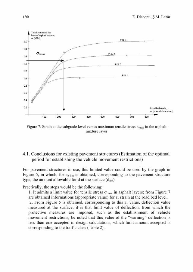
190 E. Diaconu, Ş.M. Lazăr
σrmax
Figure 7. Strain at the subgrade level versus maximum tensile stress σrmax in the asphalt mixture layer
4.1. Conclusions for existing pavement structures (Estimation of the optimal period for establishing the vehicle movement restrictions)
For pavement structures in use, this limited value could be used by the graph in Figure 5, in which, for єz lim is obtained, corresponding to the pavement structure type, the amount allowable for d at the surface (dlim).
Practically, the steps would be the following: 1. It admits a limit value for tensile stress σrmax in asphalt layers; from Figure 7 are obtained informations (appropriate value) for єz strain at the road bed level. 2. From Figure 5 is obtained, corresponding to this єz value, deflection value measured at the surface; it is that limit value of deflection, from which the protective measures are imposed, such as the establishment of vehicle movement restrictions; be noted that this value of the “warning” deflection is less than one accepted in design calculations, which limit amount accepted is corresponding to the traffic class (Table 2).

“Computational Civil Engineering 2010”, International Symposium 191
Table 2. Admissible pavement surface deflection dadm corresponding to the traffic class
Traffic class Ti
Calculation traffic, Nc, millions of standard axles
of 115 kN
Admissible pavement surface deflection dadm, 1/100 mm
Very Heavy - T1 1.00 ... 3.00 45 Heavy - T2 0.30 … 1.00 60 Middle- T3 0.10 … 0.30 65 Light - T4 0.03 … 0.10 70
4.2. Conclusions for new pavement structures (Determination of the minimum required elasticity modulus at the road bed level)
For the design of new pavement structures could be taken into account the following:
1. It admits a limit value for tensile stress σrmax in asphalt layers; from Figure 7 are obtained informations (appropriate value) for єz strain at the road bed level. 2. From Figure 6 is obtained the value of E0 (elasticity modulus of subgrade in the road bed); it is the minimum amount to be provided to the support level, thus, the pavement structure to be protected against the distress of the thaw period.
References
1. Diaconu, E., Risk assesment of inflation to frost phenomenon occurrence, National Road Congress, Timişoara, Romania, 2002.
2. Diaconu, E., Thaw barriers – solution for pavement design with respect to the action of frost-thaw phenomena, “Road and bridges rehabilitation” Symposium, Cluj Napoca, Romania, may 2007.

“Computational Civil Engineering 2010”, International Symposium Iasi, Romania, May 28, 2010
Developing the computational urban systems in Romania based on the survey data
Geanina Cosmina ADAM1, Gabriel Iulian MIHAI2 1Hydrotechnics Department, “Ovidius” University, Constantza, 900524, Romania
2S.C. Velacost S.R.L., Constantza, 900726, Romania
Summary
The importance of developing the urbanism in our country is a problem that represents a continuous preoccupation for specialized engineers and for the state institutions (town halls, financial administrations.). Nowadays, it is aimed at making urban informatics systems, using automatic calculation programs, making some complete and modern data bases that offer the necessary information to all those interested. A special importance is given to the survey field that is in a close connection to the urban system. Due to the real estate development from our country, it can be said that making a cadastral data base and an informatics urban system may certainly lead to the improvement of the relation between institutions and the real estate developers. For this purpose, it is aimed at obtaining all the necessary information referring to the urban development by making the data bases necessary to any physical or juridical entity.
KEYWORDS: data base, urban development, urban informatics system, urbanism.
1. INTRODUCTION
In order to achieve a modern urbanism, all the technical and economical data, referring to a town, need to be known. These data lead to a good communication between specialized institutions, engineers and local administrations.
The urban design supposes knowing in detail each lot in the town. For this purpose, it is necessary to have a cooperation of engineers from the urban field, constructions, survey and local administrations.
An important role in the implementation of a modern urban system is held by knowing thoroughly the survey of the town and making maps and topographical plans.

“Computational Civil Engineering 2010”, International Symposium 193
At the same time with the IT technology development, it was passed from the manual execution of plans and maps to the automatic execution.
The automatic obtaining of the cadastral plans supposes the passing to a new type of plan, that has a contents expressed by numerical and alphanumerical data, a necessary condition for the process of automation. Two possibilities of making a digital cadastral plan are distinguished:
Making a new plan - digital cadastral plan (numerical) – that has a complete contents (similar to the basic cadastral plan, including the accuracy), obtained by performing new automatic measurements, for the scale 1:500, but which needs a big consumption of time and very high expenses.
Providing a plan with more weak contents and accuracy – the index cadastral plan – that is completed with information stored in a digital archive, made by computation of the ortophotoplan and the existing cartographical and cadastral documents (at scales of up to 1:5000 including), thus with less time and financial expenses.
2. MAKING THE DIGITAL CADASTRAL PLANS USING DATA OBTAINED BY CLASSICAL AND AUTOMATIC METHODS
The digital cadastral plans are made based on the data obtained by the digitization and scanning-vectorizing the existing plans, by using the data obtained by classical and automatic instruments, using GPS technology and photogrammetry for collecting the data (fig.1).
Figure 1. Ways of obtaining the spatial

“Computational Civil Engineering 2010”, International Symposium 194
The digital cadastral plan is an integral product constituted by data and alphanumerical information, grouped by their nature and belonging in files, able to provide automatically and at any time, the partial or total graphical expression of space, at a random scale.
The points are expressed by their coordinates and two codes are associated to them:
Of Form (for line tracing) and
Of Function (necessary for the drawing and on the other hand for grouping them according to their nature)
The advantages of the digital cadastral plan:
The value of the stored information is totally guaranteed, because its preservation does not depend on a graphic drawing, which almost always is imperfect and generally has an unstable support in time;
Allows the complete automation of cadastral works, starting with collecting the data on the field, continuing with processing them, by determining their areas, applying on the field of plotting/merging by updating them and finishing with obtaining the graphical expression of the plan;
The scale is actually 1:1, so it is independent of the graphical plan scale (the entities of the digital cadastral plan are registered by their coordinates on the field) and it refers only to the degree of detail, the density of the represented entities and the accuracy in their determination;
It is very useful for performing studies and making decisions in different sectors of activity, because it allows the quick selection, through the computer, as according to the wish of the users, of the necessary information and then their automatic drawing in the form of a basic cadastral plan or thematic cadastral plans.
They are the most indicated to serve as support for the quick placement in space, in the form of thematic plans, of the big collective files, that contain economic and social data, referring to industry and the pollution phenomena of the atmosphere, to population and taxation system, etc.

“Computational Civil Engineering 2010”, International Symposium 195
The general cadastral plans from a place contain: the denomination of the administrative-territorial unit, the road network, roads, streets, alleys and railways, the hydrographic network and the important hydro technical constructions (rivers, lakes, open channels, dams, dykes), the points that mark the frontiers of the administrative-territorial unit, the limits and the denomination of the elements within the built-up area, elements of toponymy, the points in the geodetic network, the geographical north, the plan scale.
3. PERFORMING THE DATA BASES FOR OBTAINING INFORMATION FROM THE URBANISTIC FIELD
The graphical component of the data base represents the graphical support, in a digital format, of the index cadastral plan. This digital plan is made by the performer, by scanning-vectorizing the existing cartographical documents in the area, made available by the beneficiary (OJCPI). The digital plan is then completed with the elements resulting from the performed measurements in the field at the updating.
The data organized in files are stored in a data bank representing the new digital cadastral plan that can render at any time the graphical plan, at any scale (fig.2).
TAKING OVER THE DATA
THE FILE OF THE POINTS
MEASUREMENT PROCESS
DRAFT
PROCESSING THE DATA FINAL DRAFT
TEMPORARY DRAWING
THE FILE OF THE ELEMENTS
FINAL DRAWING
DATA BANK of the numerical cadastral plan (digital)
Figure 2. The chart of the technological process of taking over and processing the measured data in the field, for obtaining the digital cadastral plan

“Computational Civil Engineering 2010”, International Symposium 196
The data obtained refers to:
Setting the limits of the cadastral sectors;
Identifying the limits of the property entities, as well as the linear elements;
Executing measurements in the field for updating and completing the existing cadastral elements;
Collecting the textual elements for the property entities;
Information about buildings referring to the height, surface, destination, construction year, owners, materials that the building is made of, the technical-public utility facilities;
Data referring to the name of the streets and their facilities from a technical point of view as well as the gas network, sewerage, water, electric power and telecommunications, etc.
4. MODERN TECHNOLOGIES OF PERFORMING URBANISTIC PLANS
The digital photogrammetry represents a basic component of the modern technologies of creating and updating the topographical maps, of making the ortophotoplans, the photomaps, creating and updating the topographical and specialized plans.
The photogrammetry represents the most money saving method of collecting data for large surfaces and has lately had a period of great transformations both as far as taking over senses as well as the classical technology of the photogram and stereogram exploitation.
The purpose of the air photographing the ortophotoplans in a digital format is appropriate to the interpretation and vectorization of the plots.
The colored ortophotoplans in a digital format, are produced in the national system of reference (ellipsoid Krasovski 1940, stereo system of production 1970 and system of altitudes, Black Sea, 1975).
In order to obtain the maps and very accurate plans, applications specific to the Geographic International System are made. (G.I.S.).
The Geographic International Systems, as tools for solving the space problems, generally serve at providing reliable information necessary for

“Computational Civil Engineering 2010”, International Symposium 197
making decisions and taking action. Providing such information depends on the availability of data, on the technical possibilities of equipments and programs and on the professional level of the program user. In order to be used, the GIS must comply with the following fundamental requirements: accept the necessary data, store the introduced data, process and analyze the stored data, display the produced information.
Thus, a GIS may be defined as a collection of subsystems that comply these requirements (fig.3).
DATA PROCESSING SUBSYSTEM
Teledetection images
Primary data
Secondary data Field
measurements
DATA ACQUISITION
INTRODUCING DATA
Numerical format convention
Georeference Processing the imagesTransforming the
entities and the format
DataThe summary
of space covering
The summary of temporal
covering
STORING THE DATA
DATA ANALYSIS SUBSYSTEM
Integrating the data base Statistical analysis
Modeling
FINDING andANALYSIS
PRODUCING INFORMATION
Making reports Making maps
Displaying Numerical
data
INFORMATION USE SUBSYSTEM
Designers Researchers
USERS
Managers
MANAGEMENT SUBSYSTEM Organization
Personnel Procedures
Figure 3. The structure of a GIS (modified after H. Calkins 1988)
5. CONCLUSIONS
In the paper it is described the way of obtaining an International Urban System, as complete as possible, necessary to all the administrative-territorial institutions and specialists in the urban field.

“Computational Civil Engineering 2010”, International Symposium 198
It is referred to making a cadastral data base as complete as possible for the urban field, as well as the necessity of making cadastral plans and maps by modern technologies.
The execution of cadastral plans and topographical maps lead to identifying on the field of the necessary data to build new constructions, new railways, streets, boulevards, technical-public utility networks, green places arrangement, etc.
Thus, in order to accomplish any new objective in a town, those interested may benefit from all the necessary information, both as far as infrastructure is regarded and also the superstructure of the town.
References
1. Adam G.C., Doctor degree thesis - ,, Contributions to performing a computational urban system of a city”, March 2010. (in Romanian)
2. Petrescu F., Goegraphic computational systems in urbanism and territory arrangement, MatrixRom Publishing House, Bucharest, 2007. (in Romanian)

“Computational Civil Engineering 2010”, International Symposium Iasi, Romania, May 28, 2010
Modern specific software used in structural engineering, architecture, urbanism and town planning
Geanina Cosmina ADAM1, Gabriel Iulian MIHAI2, Anca Alina LAZĂR3 1Hydrotechnics Department, “Ovidius” University, Constantza, 900524, România
2S.C. Velacost S.R.L., Constantza, 900726, România 3Terrestrial measurements and Cadastre Department, “Gheorghe Asachi” University, Iassy700050,
România
Summary
The development of specialized engineering software for structural engineers, urbanists, town planners and architects, lead to a remarkable improvement of their activity, especially in the design process, but also in engineers collaboration with different institutions and local administration.
Due to constructions and engineering works development in the last years, the specialized engineering software had to keep up in order to facilitate the engineers activity.
The extensive capabilities, covering both engineering modeling and execution layouts, allow engineers to broaden the range of practical possible solutions avoiding a large amount of resources that would have been otherwise spent in oftenly futile laboratory works.
Allplan is the one of the latest engineer software used in constructions, architecture, urbanism and town planning.
KEYWORDS: engineers software, Allplan, constructions, architecture, urbanism, town planning.
1. INTRODUCTION
Constructions industry and urbanism are the engineering activity fields which have fully been affected by the IT technical progress. In `90 years urbanists were doing a manual design using a corbel and a compass. Presently the urbanistic design is encountering a huge step forward, both due to specific CAD and GIS software and hardware equipments.
Years 2006-2007 represent a milestone in the General Urbanistic Plans renewal process as Romania has been accepted an EU member. By adopting a GIS based solution for the GUP a match has been accomplished between fundamental studies that are realized prior to the actual GUP documentation and urbanistic design process.
200 G.C. Adam, G.I. Mihai A.A.Lazăr
By using specialized software it may be further developed: urbanistic certificates automated issuing and controlling, building authorization, demolition authorization; statistical information controlling about population, lands, economical situation; land study information controlling (earthquake, flooding, earth flow); historical monuments and touristic opportunities information controlling; spatial analysis; situation of monuments – localization, visualization and attached photos; touristic opportunities - localization, visualization and attached photos; statistics: population, education, economy, fields; territory balance.
Internet communication need the date traffic significantly increased in the last years. The diversity determined the webhosting companies to invest in infrastructure, to improve the services quality that had as effect the improvement of transfer speed. Such high technology development is GIS. As GIS tools become more complicated and accessible from cost point of view.
In the last years most of engineers and architects started to utilize the 3D modeling procedure instead of 2D one.
A 3D model contains objects, materials, layers that compose a complex structure. There can be visualized either separate or all proprieties. The objects and materials have easy to see proprieties called visual proprieties, as colour, light reflection or contrast. In the end, there can be obtained building facades, roofs or even the site 3D model.
A 3D model offers a lot of work possibilities as dimensions adjustment, constitutive components connection, creation of a new product starting with base elements. Finally, the obtained date can be integrated or exported to another specific software used for design process, town planning, tourism, security, etc.
2. APPLYING ALLPLAN SOFTWARE IN STRUCTURAL ENGINEERING, URBANISM AND TOWN PLANNING
A 3D model used for a urbanistic representation allows us to keep an „old city” view with untouched architecture or historic monuments. Thus, using a 3D model we can preserve a town view over time.
For a 3D project it can be used the land digital model made by merging photogrammetric sights and the classic topographic surveys.
The model will be a real copy of the terrain view and the „virtual” 3D city can be very easy accessed.
Actual systems facilitate the 3D model generation. It can be easily analyzed and also can be modified according to specific requirements. The design process using

“Computational Civil Engineering 2010”, International Symposium 201
a 3D model is faster and more efficient than the 2D traditional one. The big advantage is that we can visualize everything in real time and do not have to imagine the 3D model having in front of us the 2D drawings.
Allplan software made by Nemetschek is the complete design solution even for architects, structural engineers and town planners. Allplan Integra has in addition supplementary modules for the entire design process. It also has easy to use functions for landscape architecture, urbanism and other more.
Allplan Architecture is a complete solution for the entire design process. It is used for drawings erection, for 3D modeling stage, for rendering, execution details, also for determination of list of quantities.
2.1. Description of ALLPLAN application
Allplan Architecture includes:
2D structures; Extended modulus for constructions; Text; Measurement devices; Detailing windows; Drawings arrangement; Cross-sections erection; 3D modeling; Control animation; painting; Visualize; Associative views; General architecture.
Allplan Urbanism is a complex software for 2D drawings generation for urbanism and town planning (fig. 1), for maps arrangement and for buildings 3D models.
Figure 1. Plan urbanistic

202 G.C. Adam, G.I. Mihai A.A.Lazăr
Allplan Urbanism contains important tools for land drawings and digital models erection and also for volumes and surfaces computation. The most important tools include symbols, land and building occupancy factor determination.
Allplan Urbanism can be very efficiently used also in project initial stages and in the final documentation stage. It has the best tools for presenting and creating town planning plans.
Advantages:
Urbanism studies, specific maps, generation of drawings for GUP, ZUP, etc;
Specific symbols libraries;
Intelligent buildings models and different options for town planning presentation;
Automatic description of buildings and of areas;
Views, elevations and perspectives erection;
Possibility of lists and graphics generation (total areas, building and terrain occupancy factors, etc).
Allplan Engineering is a simple computer added design solution for all civil engineering domains.
Allplan Engineering contains:
2D structures; Text; Measurement devices; Detailing windows; Drawings arrangement; Cross-sections erection; 3D modeling; Macros; Control animation; 2D individual bars reinforcement; 3D individual bars reinforcement; 3D welded networks reinforcement; Automatic reinforcement quantity; Element modeling; Walls, spans, structural elements; Stairs construction; Roof modeling.
On-Site Photo (Allplan Photo) – Surveying erection
On-Site Photo allows a new method of existing buildings drawings erection based on photos.
This method makes possible the correction of photos (facades) made with a camera (fig.2).

“Computational Civil Engineering 2010”, International Symposium 203
Figure 2. Correction on facades with On Site Photo
Finally it will be obtained a plan view of the facade.
By dimensions corrections there can be determined useful dimensions of doors, windows, a facade total length, etc.
Due to possibility of determining exact building dimensions based on adjusted photos, there is no need to do any site direct measurements. All it has to be done are some representative photos with a digital camera. After that it is very easy to create a scale drawing using Allplan tools (fig.3).
Figure 3. Final facade made based on adjusted photos using On Site Photo
After the drawings are created, On-Site Survey can very easily generate important lists about all rooms which can be saved in MS Word or Excel files.

204 G.C. Adam, G.I. Mihai A.A.Lazăr
3. CONCLUSIONS
Specific software utilization in structural engineering, architecture or urbanism also for design and drawings had a very important development in the last years. These programs bring a considerable improvement to engineers activity. The present paper had described a modern specific software for both structural engineering and urbanism. Its scope is to accentuate the utility of different software in engineers activity in the way of facilitating their work.
References
1. Adam G.C., Teză de doctorat-,,Contribuţii la realizarea unui sistem informaţional urban al unui municipiu”, Martie 2010. (in Romanian)
2. ESRI, GIS for Sustainable development, December 2007
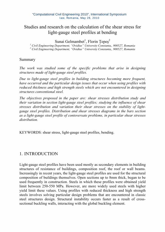
“Computational Civil Engineering 2010”, International Symposium Iasi, Romania, May 28, 2010
Studies and research on the calculation of the shear stress for light-gauge steel profiles at bending
Sunai Gelmambet1, Florin Ţepeş2 1 Civil Engineering Department, “Ovidius” University Constanta,, 900527, Romania
2 Civil Engineering Department, “Ovidius” University Constanta,, 900527, Romania
Summary
The work was studied some of the specific problems that arise in designing structures made of light-gauge steel profiles.
Due to light-gauge steel profiles in building structures becoming more frequent, have occurred and the particular design issues that occur when using profiles with reduced thickness and high strength steels which are not encountered in designing structures conventional steel.
The objectives proposed in the paper are: shear stresses distribution study and their variation in section light-gauge steel profiles; studying the influence of shear stresses distribution and variation their shear stresses on the stability of light-gauge steel profiles. Distribution and shear stresses diagrams in the bars section as a light-gauge steel profile of contoversate problems, in particular shear stresses distribution.
KEYWORDS: shear stress, light-gauge steel profiles, bending.
1. INTRODUCTION
Light-gauge steel profiles have been used mostly as secondary elements in building structures of resistance of buildings, composition roof, the roof or wall beams. Increasingly in recent years, the light-gauge steel profiles are used for the structural composition of buildings themselves. Open sections up to 8mm thick, began to be used frequently in construction. Steels in which these profiles were obtained yield limit between 250-550 MPa. However, are more widely used steels with higher yield limit these values. Using profiles with reduced thickness and high strength steels involves solving particular design problems that are encountered in classic steel structures design. Structural instability occurs faster as a result of cross-sectional buckling walls, interacting with the global buckling element.

206 S. Gelmambet, F. Tepes
Figure 1. Structure made of light-gauge steel profiles
One specific problem in designing light-gauge steel components is torsional stiffness. The light-gauge steel profiles have usually thin walls and hence a low torsional stiffness.
Figure 2. Buckling by bending-torsion

“Computational Civil Engineering 2010”, International Symposium 207
Many light-gauge steel profiles are with one symmetrical ax in sections having gliding center eccentric to the center of gravity, as shown in Figure 2a. To produce bending without torsion the loads line must pass through the gliding center section. Any eccentricity of the axle load gliding center will produce considerable torsion deformation of a thin-walled beams, as shown in Figure 2a. Sections with one axis of symmetry can lose stability by bending-torsion. Even double-symmetrical section beams, due to inefficiencies can lose stability by bending-torsion.
Where the section beam has one axis of symmetry (as in Figure 3) and plane forces
is normal to this in section develops shear stresees and in accordance with
known rules. The shear stresees are calculated with Juravski relation,
zTxy zT
xz
y
yzTz
tI
ST (1)
where:
Tz is shearing load targeted vertical axis (z)
Sy is statical moment reported at neutral axis surface in the section limited by one of the points of zero and the point where the tangential pressure is calculated
t is the thickness (normal to the median contour) profile at the point of calculating the shear stress
Iy is the moment of inertia of the all section, reported at neutral axis of the section.
Figure 3. Representation of flow shear stress in section

208 S. Gelmambet, F. Tepes
The amount shear stresses are even shear force Tz acting in „the heart” of the
beam. Amount shear stresses rise in „feet” Fy forces forming a couple of
moment (Fyh) in any point in the plan section. The moment Fyh is likely a torsion moment.
zTxz
zTxy
As a result, in such cases, bending is accompanied by a supplementary torsion section (spam). The question therefore is: To what point of the axis of symmetry should be applied load (Fz) so that turning to be avoided torsion. This point is called „gliding center” at is a distance and ec (yet unknown) of the real material support shear force Tz, of the heart profile. To determine the distance between the axis of the heart and gliding center C are reduced compared to gliding center forces result of the shear stresess. Moments resulting from this reduction Tzec and Fyh opposite.
In the absence of torsion, they must be equal and opposite.
Of equal
hFeT ycz , (2)
resulting
hT
Fe
z
yc . (3)
, (4) tmed
Tzxyy AF ·
At is sectional area the base, At = tb
and
22
·hb
ttI
T
y
zmed
Tzxy , (5)
with this
y
zy I
htbTF
4
2
, (6)
and then
y
c I
htbe
4
22
. (7)

“Computational Civil Engineering 2010”, International Symposium 209
Knowing the position (ec) gliding center is the most practical importance, if loads beams are normal to the axis of symmetry of the section. In conclusion for determining gliding center position is very important to know the flow and variation shear stresses in section. Flow chart and shear stresses diagrams representation of the section is one of contoversate problems, especially shear stress flow.
2. SIMULATIONS PERFORMED AND RESULTS
For determining shear stresses flow simulations were performed on different sections of thin sections using finite element program COSMOS 2.6. The results obtained using computer program were compared with classical results, obtained with Juravski relation.
Figure 4. Static scheme used in the simulations
Figure 5. Flow charts and shear stress diagrams

210 S. Gelmambet, F. Tepes
Figure 6. Flow and shear stress values zTxy
Figure 7. Flow and tangential stress values in section zTxy
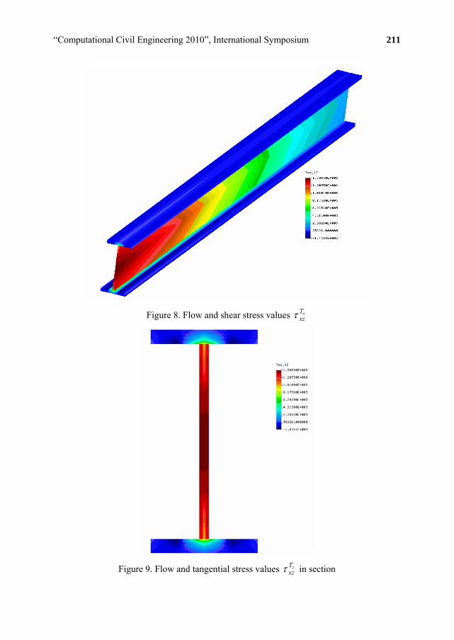
“Computational Civil Engineering 2010”, International Symposium 211
Figure 8. Flow and shear stress values zTxz
Figure 9. Flow and tangential stress values in section zTxz

212 S. Gelmambet, F. Tepes
Figure 10. Flow charts and shear stress diagrams
Figure 11. Flow and shear stress values zTxy

“Computational Civil Engineering 2010”, International Symposium 213
Figure 12. Flow and tangential stress values in section zTxy
Figure 13. Flow and shear stress values zTxz

214 S. Gelmambet, F. Tepes
Figure 14. Flow and tangential stress values in section zTxz
Figure 15. Flow charts and shear stress diagrams

“Computational Civil Engineering 2010”, International Symposium 215
Figure 16. Flow and shear stress values zTxy
Figure 17. Flow and tangential stress values in section zTxy
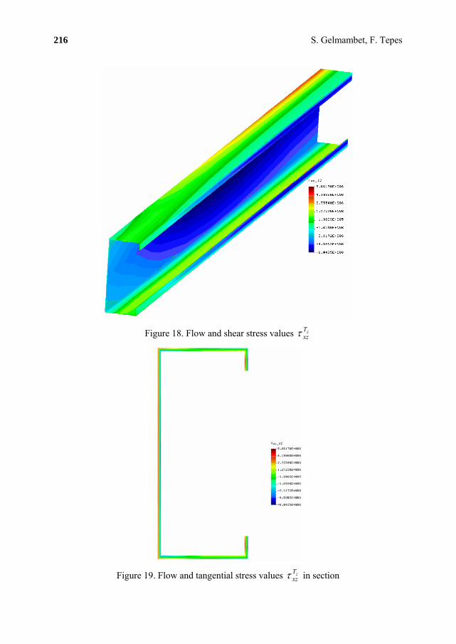
216 S. Gelmambet, F. Tepes
Figure 18. Flow and shear stress values zTxz
Figure 19. Flow and tangential stress values in section zTxz

“Computational Civil Engineering 2010”, International Symposium 217
Figure 20. Maximum values compared
3. CONCLUSIONS
In shear stresses cases (shear stress of foot), notes that the flow is not even a
linear variation. More specifically, the flow varies linearly until near the heart and then start to decline until the heart axis. Maximum values are found somewhere near the heart profile, the last third base, but not in heart profile.
zTxy
The values compared with those calculated using the relation of classic
Juravski see that we have two situations. In the case two axes of symmetry sections values calculated using relation Juravski are slightly higher which leads to an excessive dimension of the section profile.
maxxy
In the case sections with one symmetry axis Juravski calculated values are lower leading to a particular low dimension sectional profile of the loss of stability of
bending-torsion. For shear stress (shear stress of the heart) it is noted that the results are closer to the classic calculated with Juravski relation.
zTxz
As shear stresses are found in sections with two axes of symmetry maximum
values are slightly higher when using Juravski relation, and if the sections
with one symmetry axis of maximum values are calculated with Juravski
slightly lower.
zTxy
maxxz
maxxz
Variation the shear stresses is parabolic and shear stresses are maximum
values in the neutral axis as in classical calculations. Finally biggest differences are
zTxz
maxxz

218 S. Gelmambet, F. Tepes
found in shear stresses , particularly for one symmetry axis sections both in
terms of variation and in terms of determined values.
zTxy
In conclusions, bending beams require additional connections placed at different intervals, or continuously, to prevent torsion. These connections are required if the current close of sections C and Z beams, which can lose the overall stability because insufficient lateral connections.
References
1. EUROCODE 3: (EN 1993-1-1) – Elemente generale. (EN 1993-1-3) – Elemente din oţel cu pereţi subţiri formate la rece. (EN 1993-1-5) – Plăci plane încărcate în planul lor. (EN 1993-1-8) – Îmbinări.
2. Dalban C., Construcţii cu structură metalică, E.D.P. Bucureşti 1997. 3. Dubină D., Rondal J., Vayas I., Calculul structurilor metalice-Eurocode 3: Exemple de calcul. 4. Dubină D., Ungureanu V., Calculul şi proiectarea construcţiilor din profile metalice cu pereţi
subţiri formate la rece, vol.1, Colecţia LINDAB, 2004. 5. Kümbetlian G., Gelmambet S., Rezistenţa Materialelor pentru Constructori (Breviar de teorie şi
Probleme), Editura Fundaţiei „Andrei Şaguna” Constanţa, 2006. 6. G.P. 078-03, Ghid privind proiectarea halelor uşoare cu structură metalică. 7. Popescu V., Construcţii metalice, Editura Tehnică Bucureşti, 1975.

“Computational Civil Engineering 2010”, International Symposium Iasi, Romania, May 28, 2010
Improving the e-Learning of Engineering Physics with the Aid of Adobe Flash
I. Radinschi1, C. Damoc2, B. Aignatoaie3 and V. Cehan4 1Department of Physics, “Gh. Asachi” Technical University, Iasi, 700050, Romania,
[email protected] 2Faculty of Automatic Control and Computer Science, Iasi, 700050, Romania,
[email protected] 3 Faculty of Automatic Control and Computer Science, Iasi, 700050, Romania,
[email protected] 4 Faculty of Electronics, Telecommunications and Information Technology, “Gh. Asachi” Technical
University, Iasi, 700506, Romania, [email protected]
Summary
Computer-assisted teaching and learning methods have significantly developed over the last years, leading to effective results for physics courses and laboratories. We apply computer graphics for teaching and learning physics through the use of computer simulations and the e-learning process. Our methods which involve the use of computer simulations in order to study physics phenomena rely on Adobe Flash CS3 software, giving students the opportunity to understand better the phenomena in the world of physics. We have implemented these computer simulations of the physics phenomena in the e-learning process providing rapid access by creating a Virtual Physics Lab. Our simulated experiments are developed using the data gathered from real physical experiments, and describe with a high degree of accuracy the behavior of the laboratory equipment. The computer applications can be accessed via Internet using a mobile phone, a computer or a laptop from any location.
KEYWORDS: engineering physics, e-learning, Adobe Flash.
1. INTRODUCTION
The combination of traditional teaching - learning methods with computer-assisted methods integrated in the e-learning environments [6], [8], [9], [10], [11], [12], [13], [14], [16] leads to an improvement of the educational process. This integration can be developed even further via the implementation of computer-based learning technologies. Significant efforts have been made both in our country and abroad, in order to integrate appropriate software for the use of computer graphics and animation in the educational process.
Computational programs are increasingly used in engineering education, ensuring the integration of state-of-the-art software which allows the simulation of experiments in the study of physics phenomena [1], [2], [3], [4], [5], [7], [15], [18].

220 I. Radinschi, C. Damoc, B. Aignatoaie and V. Cehan
Due to the experience gathered in the field of physics [7]-[14], [18] it is now understood that computer simulations are extremely useful for data processing.
As far as the constant improvement of our physics classes and laboratory activities are concerned, the description and animation of physical phenomena with the help of computer simulations is of utmost importance. The implementation of these techniques in the educational process [7], [9], [10], [11], [12], [13], [14], [17], [18] will enable students to understand better the physics phenomena and to check the findings of their experimental work. Students will be taught how to operate this software in order to explore, assimilate and apply the laws of physics, and in this process they will develop their measurement and analysis skills. Our computational tools use Java and Adobe Flash CS3 [10] software and the applications are continuously updated and optimized. After the implementation of these tools, our students have become more interested in learning physics and are far more motivated.
Since computer simulations are error free, they can be employed as verification tools in the laboratory, allowing the checking of the findings of experimental works. In order to provide a better and faster use of our set of computer physics simulations, we have also developed an e-learning environment, based on a Virtual Physics Lab that contains simulated experiments elaborated in Adobe Flash CS3 and a Chat window that enables the students – teachers and students – students discussions. The e-environment allows students to access, work and change opinions using electronic devices like cell phones and laptops. Thus they can perform various experiments directly in the Virtual Physics Lab and make a comparison with the results obtained in the real physics laboratory.
2. COMPUTER SIMULATIONS AND THE VIRTUAL PHYSICS LAB
We have been using the Adobe Flash CS3-based computer simulations in our physics laboratory activities since 2008. Before 2007, we used the Java program for our simulated physics experiments.
Due to its flexibility and advanced graphical features, the animation and programming environment of Adobe Flash CS3 is ideal for the elaboration of simulations. This state-of-the-art software contributes to the creation and processing of numerous applications, animations and web pages. The users who develop Flash applications can benefit from special possibilities thanks to the operations, functions and user friendly characteristics of this software. Thus, Flash stands out as a robust and interesting environment for developing applications.
Together with our students, as a first step, we established the most suitable works for computer simulations. After deciding on the priority order of these experiments, we conceived the computer simulations in such a manner as to

“Computational Civil Engineering 2010”, International Symposium Iasi, Romania, May 28, 2010
221 generate the same results as the experimental findings. By using the experimental data collected from certain points during a fixed time period, an interpolation of first degree was implemented in these computer simulations. In order to obtain the results we use necessary physical formulas and laws.
Consequently, the user is given the possibility of analyzing simulation values within the same time period as that of the real physics experiment. The user can thus select a value, without having to stick to a limited number of values or only to experimental values. The students can make comparisons between practical experiments and simulations.
The simulated experiments were elaborated such as each package contains a screen-shot with the presentation of the physics laws and phenomena and apparatus both in English and in our mother tongue, and one or more graphic interfaces of the effective simulation of the laboratory work. These computer simulations also enable students to verify experimental data, using formulas and plot graphs.
With the help of Adobe Flash CS3 program, we have managed to create several interactive simulated physics experiments [6]-[7] meant to illustrate some essential aspects of physics phenomena and laws, such as: black body radiation, the photoelectric effect, the determination of Planck’s constant, the study of electromagnetic waves, the study of polarimeter, the study of the thermal activation energy of intrinsic conduction for a semiconductor, and others. In this way, we have provided an interactive learning process and we have at our disposal a set of different simulations related to a series of physics phenomena, which detail numerous aspects of physics that are dealt with in our course.
As an example, we consider the computer simulation elaborated for the study of the dependence between the photoelectric current intensity and the illuminance in the case of the photoelectric effect, at constant values of the
voltage [6]. This computer application has an interface which describes the lab objectives and the procedure and other interfaces for the graph representations. The
law is studied in the same computer application together with the
current – voltage curve, which is given by the
.)( constUf EfI
(f UfI
U
)( UE .constf fI
.) constE dependence.
The computer simulation allows the construction of the graph .)( constUf EfI .
The students have to choose a constant value for the voltage U and taking into account a constant value for the luminous intensity cdI 1 , they enter the values for the distance between the source of light and photoelectric cell picking up the corresponding values for the photoelectric current intensity. For this application we give an example of the source code bellow:
function myDraw():void { var r_aux:Number = 0;

222 I. Radinschi, C. Damoc, B. Aignatoaie and V. Cehan
var r_offset:Number = rSlider_mc.minimum; var r_samples:uint = arr_r.length; var I,j,k:uint = 0; var myX,myY:int = 0; var myfrac:Number = 0; gLine_mc.graphics.clear(); gLine_mc.graphics.lineStyle(1, 0xFF3300, 0.8); gPoint_mc.graphics.clear(); gPoint_mc.graphics.lineStyle(1, 0x000000, 1); r_aux = r_offset/100; E = 1/(r_aux*r_aux); my_if[0] = arr_If[0]; myX = Math.round(20*E); myY = -Math.round(32*arr_If[0]); gLine_mc.graphics.moveTo(myX, myY); gPoint_mc.graphics.beginFill(0x000000); gPoint_mc.graphics.drawCircle(myX, myY ,1); gPoint_mc.graphics.endFill(); for(k=1; k<=70; k++) { r_aux = (r_offset + k)/100; //trace(r_aux); E = 1/(r_aux*r_aux); //trace(E); for(j=0; j<r_samples; j++) { if(arr_r[j] > r_aux) break; } j=j-1; if(j >= r_samples-1) { my_if[k] = arr_If[r_samples-1]; } else { myfrac = (r_aux – arr_r[j]) / (arr_r[j+1] – arr_r[j]) ;
my_if[k] = arr_If[j] + myfrac * (arr_If[j+1] – arr_If[j]) ; //trace(k + “ “ + my_if);}

“Computational Civil Engineering 2010”, International Symposium Iasi, Romania, May 28, 2010
223
myX = Math.round(20*E); myY = -Math.round(32*my_if[k]); gLine_mc.graphics.lineTo(myX, myY); gPoint_mc.graphics.beginFill(0x000000); gPoint_mc.graphics.drawCircle(myX, myY ,1); gPoint_mc.graphics.endFill();} }
We posted our physics course on the Internet in 2007 and this year we decided
to implement our set of computer simulations in the e-learning process developing an e-learning platform for our laboratory classes. Our aim was to develop a Virtual Physics Lab based on computer simulations of physics phenomena. In this way, our set of simulated laboratory works can be performed from a distance by logging on our website and working in our Virtual Physics Lab. These simulated experiments have been developed for our students of technical engineering, but they can also be used by the students of the Faculty of Physics. Password protected access can be also extended to other users for providing information.
This virtual learning environment allows the use of multimedia technologies through images, text and simulations. Further, on this web page we give the students the possibility to use the computer simulations directly from the Internet, which provides inexpensive and fast access study materials. The users can use their cell phones, computers or note-books to connect to the Virtual Physics Lab. The web page was elaborated using the Microsoft Office FrontPage 2003 editor.
In Fig. 1 we present the homepage of the Virtual Physics Lab. The web page can be accessed at the address: http://physics.phys.tuiasi.ro/~iradinsc/simulations/index1.htm. To enter in the Virtual Physics Lab the students have to log in using a username and a password. The simulated physics experiments are available all the time on the Internet and the students can practice from their rooms, Internet points available in the campus or any other location. The virtual learning environment can be used before or after working in the real physics laboratory and allows students to make a review of the concepts taught during the lectures. As a first step, we encouraged our students to work firstly in the real physics laboratory and after this to use the computer simulations. After they became more familiar with the content of the course and the laboratory equipment, they were also able to use the simulated experiments before or even during the collection of experimental data. Working in the Virtual Physics Lab demands of the students a greater level of concentration and autonomy than traditional learning methods.

224 I. Radinschi, C. Damoc, B. Aignatoaie and V. Cehan
Fig. 1 Computer simulations in the Virtual Physics Lab
The web page is connected to the one which is owned by our faculty and department, respectively. The students can use the simulations directly on the web page or they are allowed to download them onto their own computers for practice. In addition, a Chat window facilitates the communication between the students and the teacher and also between students. In this way, the students focus their attention both on the use of the physics simulations and on the changing of ideas and comments with the instructor and other students, and are highly motivated to get involved in online debates. Thus the site offers online discussions, possibilities of proposals for improvement and two-way interaction. The administration and maintenance of the on-line learning resources can be made in an easy way and without high costs or use of a complicated hardware infrastructure.
3. CONCLUSIONS
We consider that the use of computational programs to create computer simulations of physics phenomena is a significant innovation in science education. Moreover, the e-learning activity makes learning tasks more effective. This educational effectiveness based on the use of computer simulations combined with the

“Computational Civil Engineering 2010”, International Symposium Iasi, Romania, May 28, 2010
225 implementation of the online learning process matches the increasing students’ needs and their interest in this way of working.
We solve the learning tasks by direct interactions with our students in the real physics laboratory classes, and also through the use of Internet and e-learning activities in our Virtual Physics Lab. We developed this open portal where any student can download and use the computer simulations for processing experimental data, and practice his knowledge in a virtual environment for a deeper understanding of the physics laws and phenomena. The Virtual Physics Lab allows the students to perform simulated experiments, to compare the results with those obtained working directly in the real laboratory, to ask questions and communicate with the instructor and other classmates. This e-learning environment also enables controlled access to the e-learning resources. It can host a large number of users and is compatible with Windows XP, Vista and others. In this way, we promote the dissemination and popularization of physics e-learning to our students allowing a greater flexibility in organizing time for all the users involved in the use of the online resources.
In the future, in order to obtain the most satisfactory results and to maintain the learning activity as an ongoing process we intend to increase our offer and develop more computer simulations for describing other physics laws and phenomena. We will also develop the Virtual Physics Lab environment by introducing a Forum window for quick communication among the students and with the teacher, sharing ideas for future developments and collecting suggestions concerning our virtual lab. We also intend to introduce another page that will contain information about the students, such as their names and e-mail addresses. As a further step towards our goal of improving the e-learning of physics, we want to allow students to prepare online problems posting a set of computer-simulated problems connected to the experimental works on the web page.
References 1. A. Jones and K. Issroff, “Learning technologies: Affective and social issues in computer supported collaborative learning”, Computers & Education, Vol. 44, No. 4, pp. 395-408, Apr. 2005. 2. B. G. Murariu and D. Toma, “A note about the simulation programs for heat and molecular physics laboratory”, xxx.lanl.gov physics/0505053 3. G. Murariu, “Interactive computer simulations of electrokinetic physics phenomena”., xxx.lanl.gov physics/0609215 4. S. Hennessy, R. Deaney, and K. Ruthven, “Situated expertise in integrating use of multimedia simulation into secondary science teaching”, International Journal of Science Education, Vol. 28, No. 7, pp. 701-732, June 2006. 5. I. Radinschi and B. Ciobanu, “Physics studies - Computational methods, a strong connection”, in Proc. of International Symposium Computational Civil Engineering 2007, CCE 2007, Iasi, Romania, 2007, pp. 200-211.

226 I. Radinschi, C. Damoc, B. Aignatoaie and V. Cehan
6. I. Radinschi and C. Damoc, “Computer simulations for physics laboratory”, in Proc. of the Sixth International Symposium „Computational Civil Engineering 2008”, CCE 2008, Iasi, Romania, 2008, pp. 441-447. 7. I. Radinschi, C. Damoc, A. Cehan, and V. Cehan, “Computer simulations of physics phenomena using Flash”, in Proc. of the 5th International Conference on Hands-on Science Formal and Informal Science Education, HSCI 2008, Espaço Ciência, Olinda-Recife, Brasil, 2008, pp. 147-152. 8. I. Radinschi, M. D. Frunza, and B. Ciobanu, “Online virtual model for testing the knowledge”, in Proc. of INTED 2007, Valencia, Spain, 2007, pp. 42-47. 9. R. F. Wisman and K. Forinash, “Science in your pocket”, in Proc. of the 5th International Conference on Hands-on Science Formal and Informal Science Education, HSCI 2008, Espaço Ciência, Olinda-Recife, Brasil, 2008, pp. 180-187. 10. http://www.java.com/en; www.adobe.com/products/flash 11. P. R. Smith and D. Pollard, “The role of computer simulations in engineering education”, Computers & Education, Vol. 10, No. 3, pp. 335-340, July 1986. 12. T. de Jong, “Computer Simulations: Technological advances in inquiry learning”, Science, Vol. 312, No. 5773, pp. 532-533, Apr. 2006. 13. www.myphysicslab.com, http://virlab.virginia.edu 14. http://phet.colorado.edu, http://wildcat.phys.northwestern.edu 15. R. R. García, J. S. Quirós, R. G. Santos, S. M. González, and S. M. Fernanz, “Interactive multimedia animation with Macromedia Flash in Descriptive Geometry teaching”, Computers & Education, Vol. 49, No. 3, pp. 615-639, Nov. 2007. 16. H. Gould, J. Tobochnik, and W. Christian, An Introduction to Computer Simulations Methods: Applications to Physical Systems, 3rd. ed., Addison-Wesley, 2007. 17. G. Andaloro, V. Donzelli, and R. M. Sperandeo-Mineo, “Modelling in Physics teaching: the role of computer simulation”, International Journal of Science Education, Vol. 13, No. 3, pp. 243-254, Sept. 1991. 18. Kuo-En Chang, Yu-Lung Chen, He-Yan Lin, and Yao-Ting Sung, “Effects of learning support in simulation-based physics learning”, Computers & Education, Vol. 51, No. 4, pp. 1486-1498, Dec. 2008.

“Computational Civil Engineering 2010”, International Symposium Iasi, Romania, May 28, 2010
Standard vs. time-domain approach for seismic performance analysis of tall buildings
Mihail Iancovici1, Bogdan Ștefãnescu2,3
1Department of Mechanics, Statics and Dynamics of Structures, Technical University of Civil Engineering (UTCB), Bucharest, 020396, Romania
2Department of Steel Structures, Technical University of Civil Engineering (UTCB), Bucharest, 020396, Romania
3 National Center for Seismic Risk Reduction (NCSRR), Bucharest, 021652, Romania
Summary
In the last years, the increasing number of tall buildings- built in dense urban and historical areas in Bucharest, drew the attention on the seismic analysis and design framework applicable to these particular structures. While the reinforced concrete Carlton Building (14 stories) collapsed during the November 10, 1940 earthquake (Mw=7.6) and about 32 medium-rise buildings were destroyed by the March 4th 1977 earthquake (Mw=7.4) in Bucharest, there is no any evidence how highly flexible structures will perform on medium-soft soil conditions in the Bucharest-city under Vrancea source-induced strong ground motions. The current seismic design procedure in the Romanian standard (EC 8 format) is little to no applicable to tall buildings. Full analysis procedures in the time-domain are not yet available in a standardized manner. This approach may lead to inappropriate performance and highly exposed to seismic risk structures. The objective of the paper is to analyze the seismic loads distribution and standard response parameters, obtained by two approaches: (i) actual code provisions and (ii) time-history analysis using compatible artificial ground motion accelerograms database. A large number of parametric studies on 60 story models are performed. The results are emphasizing the limitations of the current approach and the availability of time-history “exact” approach, thanks to large hardware and software capabilities.
KEYWORDS: tall building, accelerogram, design spectrum, seismic performance
1. INTRODUCTION
In the last years, the increasing number of tall buildings built in dense urban and historical areas in Bucharest, drew the attention on the seismic analysis and design framework applicable to these particular structures.

228 M. Iancovici, B. Ștefãnescu
In the modern era, the reinforced concrete Carlton Building (14 stories) collapsed during the November 10, 1940 earthquake (Mw=7.6) and about 32 medium-rise buildings were destroyed by the March 4th 1977 earthquake (Mw=7.4) in Bucharest. The standard seismic analysis procedure - based on equivalent static loads using the response spectrum method approach and inelastic response reduction factors, is little to no applicable to tall buildings. It may not accurately grasp important features of both - ground motion and structure: the ground motion amplitude, frequency content and duration characteristics, directionality, the mass and stiffness distribution, damping distribution, material and geometric nonlinearities, the soil-structure interaction and site effects, the effect of incorporated energy dissipation devices etc. This approach may lead to inappropriate performance, cost non-effective and highly exposed to seismic risk structures. Very little guidance is offered in the Romanian design code for selecting/scaling/generating appropriate time-series of ground acceleration. Real records are mostly used by practitioners for behavior checking purposes rather than for analysis and design. A large variety of shapes and complex structural layouts are nowadays proposed (Gavrilescu, 2009). Consequently, the structural designers have to think technical and cost-effective solutions in order to fulfill the complex architectural needs, the owner demands and provide appropriate structural robustness to multi-hazard sources: wind, earthquake, impact, explosions etc. (fig.1).
Figure1. Innovative proposals of highly irregular shapes and complex structural layouts The analysis methods applicable to complex structures have been considerably improved. Thanks to modern measurement techniques and experimental investigation tools, important steps were made toward accurate modeling of loads and structural properties and on the enhancements of robust numerical procedures as well. In the structural dynamics, in the wind engineering field, the concept of database-assisted design was initially developed for low-rise buildings (Whalen et al., 2000). Later, this approach was extended to tall buildings (Simiu et al., 2003). This

“Computational Civil Engineering 2010”, International Symposium 229
concept can be successfully applied for seismic applications and can provide a higher accuracy in estimating the structural demand (Iancovici et al., 2009) and hence generate safer and higher cost-effective structures. The objective of our paper is to evaluate the limitations of the current analysis procedure. We compare the results obtained by the design response spectrum approach with those obtained by a large number of time-history analyses using databases of compatible time-series of ground acceleration. We also discuss the applicability of time-domain approach for seismic performance evaluation.
2. PERFORMANCE-BASED SEISMIC DESIGN OF TALL BUILDINGS
The seismic performance concept (SEAOC, 1995) consists of tuning the structural and the earthquake ground motion properties in order to obtain an accurate behavior prediction associated to certain pre-defined limit states (e.g. Serviceability, Reparability, Life Safety), making use of vulnerability and risk analyses. For tall buildings seismic design, various proposals were made for setting-up appropriate ground motion characteristics (usually the PGA associated to a mean return interval- MRI/probability of exceedance in t years) and associated standard structural performance parameters (usually expressed in terms of drift ratios). For instance Los Angeles Tall Buildings Structural Design Council (LATBSDC, 2008) suggests the following performance levels to be taken into account when tall buildings are to be designed: Level 1- building remains operational (elastic behavior) for frequent ground motions (MRI=43 yr.), and Level 2- very low probability of collapse in the case of maximum credible earthquake (MRI=2475 yr.)- as defined by ASCE 7-05. The basic approach used by practitioners for seismic loads evaluation and the induced effects is the response spectrum method due to simplicity of use and fairly good accuracy for a large class of common structural types. Demand values are obtained by standard structural analysis software, using common statistical maxima combination rules (e.g. 30%, SRSS, CQC, CQC3). The time-history response analysis accounts for the ground motion characteristics and structural properties and provides the full range of instantaneous and peaks of response parameters (loads, displacements, velocities, accelerations, internal forces, energies) that allow higher accuracy results and use of comprehensive probabilistic analysis tools. While in the case of response spectrum method approach, demand seismic loads are obtained accounting for importance factor, ground motion and structural dynamic and inelastic properties in conjunction with the mean return interval of an earthquake ground motion, in the case of time-history approach, the selection of

230 M. Iancovici, B. Ștefãnescu
appropriate ground motion time-series is a sensitive and complex issue-especially for the case of “significant motions”- from the structural viewpoint. In the Romanian seismic design code P100-1/2006 (EC 8 format), a single level of structural performance is explicitly stated. This addresses to the ultimate limit state (life safety) and the prescribed peak ground acceleration is associated to 100 yr. MRI. A serviceability limit state is used for initial structural conformation checking purposes (MRI = 30 yr.). Conceptually the standard code provisions intend to generate a uniform design for a large class of common structures. This would not necessarily produce risk-consistent structures and the associated cost effectiveness is usually not a key-issue. When tall, complex buildings are to be designed, the serviceability level becomes much more important and the safety level- a major issue. Thus, a refinement of seismic excitation characterization for various performance levels is necessary based on a large amount of available data.
2.1. The input ground motion for response analysis
The alternate approach to standard response spectrum analysis is to use appropriate site-dependant ground motion accelerograms. These can be obtained by various existing techniques: (i) recorded accelerograms; (ii) simulated accelerograms at various ground levels based on the bedrock records and soil profile; (iii) methods based on source properties, using semi-empirical Green’s function (Irikura, 1983) and theoretical simulation of fault process or using the attenuation relationships of ground motion parameters; (iv) simulated ground acceleration at free field, compatible with a prescribed time-history anvelope, Fourier amplitude spectrum/power spectrum and (v) artificial accelerograms compatible with an acceleration response spectrum/design spectrum (Gasparini et. al, 1976; Vanmarcke et. al, 1976). The use of one or another technique may raise various questions. For instance, the realistic character of time-series compatible with a design spectrum covering a wide range of natural periods with constant spectral accelerations (e.g. from 0.16 s to 1.6 s, corresponding to the soft soil conditions case in P100/2006 Romanian code) can be seriously questionable. The instrumental period- starting just after the 1977 Vrancea earthquake, provides a very limited number of significant records. However essential information from past events can be used for generating credible, realistic synthetic motions. When the performance format is the analysis goal, then ‘pointy” approaches in estimating the ground motion properties are to be used. Using the procedure proposed by Gasparini et al. (1976), for the purposes of our study we generated a large number (40 series for each case) of 1% damping ratio design spectrum compatible accelerograms with similar frequency content and duration characteristics as the possible real ones, corresponding to various soil

“Computational Civil Engineering 2010”, International Symposium 231
conditions and hazard level. The control power spectral density functions are shown in the fig. 2.
PGA = 0.24 g | Tc = 0.7 s PGA = 0.24g | Tc = 1.0 s PGA = 0.24g | Tc = 1.6 s
0 0.5 1 1.5 2 2.5 3 3.5 4 4.5 50
0.02
0.04
0.06
0.08
0.1
0.12
0.14
0.16
0.18
0.2
Frequency,Hz
PS
D,m
2/s
3
0 0.5 1 1.5 2 2.5 3 3.5 4 4.5 50
0.05
0.1
0.15
0.2
0.25
0.3
0.35
Frequency,HzP
SD
,m2
/s3
0 0.5 1 1.5 2 2.5 3 3.5 4 4.5 5
0
0.1
0.2
0.3
0.4
0.5
0.6
0.7
Frequency,Hz
PS
D,m
2 /s3
PGA = 0.36g | Tc = 0.7 s PGA = 0.36g | Tc = 1.0 s PGA = 0.36g | Tc = 1.6 s
0 0.5 1 1.5 2 2.5 3 3.5 4 4.5 50
0.05
0.1
0.15
0.2
0.25
0.3
0.35
0.4
0.45
Frequency,Hz
PS
D,m
2/s
3
0 0.5 1 1.5 2 2.5 3 3.5 4 4.5 5
0
0.1
0.2
0.3
0.4
0.5
0.6
0.7
Frequency,Hz
PS
D,m
2/s
3
0 0.5 1 1.5 2 2.5 3 3.5 4 4.5 50
0.2
0.4
0.6
0.8
1
1.2
1.4
1.6
1.8
Frequency,Hz
PS
D,m
2 /s3
Figure 2. Control PSD functions of the simulated ground motion accelerograms
One can observe that the signal’s power and the frequency bandwidth indicator ε (Kramer, 1996) are very sensitive both to PGA and Tc. However the stability of ground motion parameters for a certain case is good while the peak ground displacement is more sensitive (table 1, for 0.24g case only).
Table 1.Statistics of artificial ground motion accelerograms parameters (PGA = 0.24g)
Tc = 0.7 s
PGA ,m/s/s PGV, m/s PGD,m Tp, s ε
Mean 2.354 0.389 0.819 0.760 0.934
σ 0.000 0.064 0.392 0.112 0.003
CoV 0.000 0.164 0.479 0.148 0.003
Tc = 1.6 s
PGA ,m/s/s PGV, m/s PGD,m Tp, s ε
Mean 2.354 0.513 1.191 1.024 0.959
σ 0.000 0.085 0.628 0.128 0.002
CoV 0.000 0.165 0.527 0.125 0.002 In the response analysis the influences of various error types are to be taken into account: numerical errors from the time series generation process, errors from the

232 M. Iancovici, B. Ștefãnescu
spectral shape approximation and errors from the integration of differential equations of motion.
3. TIME-DOMAIN VS. STANDARD ANALYSIS APPROACH
Seismic loads and induced effects are obtained by two approaches: (i) the spectral approach based on elastic design acceleration response spectrum and use of maxima superposition rules and (ii) the time-domain “exact” approach, using a large number of compatible accelerograms. We compare the structural response parameters using both approaches, as well as we study the sensitivity of time-history response to soil conditions. Finally, the analyses are focused on the structural element. Numerical example 1
A generic 60 story model is considered, consisting of a central core and outer gravity frames (fig.3). The plan dimensions are Lx=36m, Ly=36m and the total height of 210 m, having 3 DOF/floor. For the sake of comparison, the model is assumed to behave linearly-elastic so that the results are not to be affected by various nonlinear effects. A Rayleigh damping model is used and the damping ratio for the first two translational vibration modes is assumed as 1%. The distribution of stiffness in elevation is linear.
CENTRAL CORE
FRAMING SYSTEM
x CSk
CMk
y
z
Lx
Ly
ex,k
ey,k
CENTRAL CORE
FRAMING SYSTEM
STORY k
Figure 3. 60 story model and typical floor plan The first natural periods in the x- and y-direction are 6.5 sec. Since the model is plan-symmetric, the set of accelerograms corresponding to PGA of 0.24g and soft soil conditions (Tc = 1.6 s) was applied in the x-direction only. This hazard level would probably correspond to the “operational level” in the future version of the code, applicable to tall buildings. The results are shown in the fig. 4 and 5.

“Computational Civil Engineering 2010”, International Symposium 233
3000 4000 5000 6000 7000 8000 9000 10000 11000 120000
10
20
30
40
50
60
Load x-dir,kN
Sto
ry
-1 -0.5 0 0.5 1 1.5 2 2.5 3 3.50
10
20
30
40
50
60
Drift ratio x-dir,%
Sto
ry
0
10
20
30
40
50
60
0 2000 4000 6000 8000 10000
Story
Load, kN
SRSS1‐10
mean th
mean+1stdv
0
10
20
30
40
50
60
0 0.5 1 1.5 2 2.5
Story
Drift ratio, %
SRSS16
mean th
mean+1stdv
Figure 4. Story seismic loads and story drift ratios, x-direction
The mean seismic loads distribution is underestimated up to 60%-for the base stories and overestimated up to 33%- for the middle stories. The mean drift ratios are severely overestimated as well as in the case of mean story shears and bending moments- up to 65% in the lower stories (fig.5).
0
10
20
30
40
50
60
0 20000 40000 60000 80000 100000
Story
Shear force, kN
SRSS15
mean th
mean th+1stdv
0
10
20
30
40
50
60
0 2000000 4000000 6000000 8000000
Story
Bending moment,kNm
mean th
SRSS1‐5
mean th+1stdv
Figure 5. Story shears and bending moments, x-direction
The statistics of time-history analyses is presented in the table 2.

234 M. Iancovici, B. Ștefãnescu
Table 2. The variability of peak response parameters from time-history analyses
Parameter CoVmax Story
Story seismic load 0.357 54
Drift ratio 0.556 21
Story shear force 0.766 60
Story bending moment 0.703 60 One can observe that the story seismic loads have the smallest variability among other parameters.
3.1. The influence of ground conditions
The ground conditions has considerable influence on the story seismic loads distribution as well as on the displacements demand. In the fig. 6 are plotted the mean values of peak story seismic loads and response parameters corresponding to PGA of 0.24g and Tc = 0.7s compared to those corresponding to same peak ground acceleration but soft soil conditions (Tc = 1.6s).
0
10
20
30
40
50
60
0 2000 4000 6000 8000
Story
Load, kN
mean 0.7s
mean 1.6s
0
10
20
30
40
50
60
0 0.2 0.4 0.6 0.8 1 1.2 1.4
Story
Drift ratio, %
mean 0.7s
mean 1.6s
0
10
20
30
40
50
60
0 10000 20000 30000 40000 50000 60000
Story
Shear force, kN
mean 0.7s
mean 1.6s
0
10
20
30
40
50
60
0 1000000 2000000 3000000 4000000 5000000 6000000
Story
Bending moment,kNm
mean 0.7s
mean 1.6s
Figure 6. Mean of peak story seismic loads, drift ratios and internal forces, x-direction The story internal forces (shears and bending moments) are little influenced by the ground condition.

“Computational Civil Engineering 2010”, International Symposium 235
Numerical example 2
For detailed information about induced effects (axial, shears, bending moments, drift ratios etc.) for individual structural elements (columns, girders, braces etc.) a full steel structure model is used. It consists of braces- macro X on 8 stories, placed on the outer frames on both main directions to resist lateral forces and inner frames to resist gravity loads. The cross-sections of columns and braces are boxes and the beams are built-up I-shapes. The structure was pre-designed for a hazard level of 0.36g (MRI = 475 yr., Bucharest) and soft soil conditions (Tc = 1.6 s). This would probably correspond to the “life safety” performance level in the future version of the code, applicable to tall buildings.
analyzed columns
Figure 7. 60 story building full model
The columns are treated as non-dissipative members, so they were sized to resist loads generated by an amplified seismic load that takes into account the estimated plastic reserve in the potentially plastic zones and the steel over-strength in these zones, according to EN 1998-1 and Romanian seismic design code. A number of 15 synthetic accelerograms compatible with the corresponding design elastic response spectrum were applied in the x-direction. In the figure 8 are plotted (i) the elastic acceleration design spectrum and the mean of acceleration response spectra (on left side) and (ii) the elastic displacements design spectrum and displacements spectra (on right side).

236 M. Iancovici, B. Ștefãnescu
0
2
4
6
8
10
12
14
16
0 1 2 3 4 5 6 7 8
SA
,m/s
/s
T,s
mean th
code
0 1 2 3 4 5 6 7 80
0.5
1
1.5
2
2.5
3
T, s
SD
,m
σ max = 0.95 CoV max =0.13
Figure 8. Design and response acceleration (mean) and displacements spectra (15 accelerograms)
Bending moments at the columns base on the same vertical (fig.7) in the x-direction were computed and the results corresponding to 5 time-series and the ratios of mean of maxima from time-history analysis (for all 15 series) to response spectrum approach are plotted in the fig.9.
0
100
200
300
400
500
600
700
800
900
0 1000 2000 3000 4000 5000 6000
spec
th1
th2
th3
th4
th5
Bending moment, kNm
Column index
0
100
200
300
400
500
600
700
800
900
0.00 0.50 1.00 1.50 2.00 2.50 3.00
Bending moments ratio
Column index
Figure 9. Base bending moments in the analyzed columns and time-history to spectrum
ratios The results are showing a severe underestimate by response spectrum approach and a large variability of ratios as well. The maximum value of the mean ratio is 2.45 and the minimum value is 0.99. While the stability in the seismic excitation characteristics is good, the time-history response variability is large (CoVmax=1.62, CoVmin=1.14); the mean ratio of base bending moments in the columns is 1.98.
4. PERFORMANCE EVALUATION IN THE TIME-DOMAIN
APPROACH The Capacity Spectrum Method (Freeman, 1970) is largely used for the evaluation of existing structures or a newly designed ones, to identify damage states, and correlate damage states to various amplitudes of ground motion. Later, the

“Computational Civil Engineering 2010”, International Symposium 237
Incremental Dynamic Analysis (IDA, Vamvatsikos and Cornell, 2003) was proposed in order to catch the structural capacity from its full dynamic properties. The use of an equivalent SDOF might be too simplified, little applicable to tall buildings. For complex structures, the full FEM model in conjunction with a large database of appropriate ground motion accelerograms corresponding to different performance levels allows the use of stochastic tools for high reliability analysis and design. Any number of those 6 ground acceleration components can be incorporated. If the internal forces are of interest, the demand to capacity ratio would control de structural design through the design interaction formulae for steel structures given in Eurocode 3 and LRFD. A large amount of data regarding the structural capacity can be obtained by efficient Monte Carlo simulation technique. If the response parameters are the drift ratios- threshold limit states are given (e.g. Eurocode 8, section 4.4.3.2), then the displacement- based control format can be directly addressed for various performance levels. The influence of ground motion directivity can be straightforward accounted for, by an incremental directional procedure (Iancovici et al., 2009). This addresses especially for irregular structures in which the main direction of motions are not obvious. For instance, a 25% (from the radius of gyratyion) equal story stiffness eccentricity ratios in both directions of the generic model is considered (fig.7). A set of artificial orthogonal ground motion accelerograms corresponding to soft soil conditions and PGA of 0.24g is applied under a 10o incremental directivity. Time-histories of induced effects are obtained from all the directions. In the fig.10, time-histories of the 10th story drift ratios in the x- and y-directions corresponding to ground motion from 20o and 320o measured form the x-direction, counter-clocwise.
20o directivity 320o directivity
0 5 10 15 20 25 30 35 40-1.5
-1
-0.5
0
0.5
1
1.5
time,s
Drift ra
tio x-d
ir, %
0 5 10 15 20 25 30 35 40-0.8
-0.6
-0.4
-0.2
0
0.2
0.4
0.6
time,s
Drif
t ra
tio x-d
ir,%
0 5 10 15 20 25 30 35 40-0.8
-0.6
-0.4
-0.2
0
0.2
0.4
0.6
0.8
time,s
Drif
t ra
tio y-d
ir,%
0 5 10 15 20 25 30 35 40-1.5
-1
-0.5
0
0.5
1
1.5
time,s
Drif
t ra
tio y-d
ir,%
Figure 10. Time-histories of drift ratios (%) in x- and y- directions, for a set of orthogonal ground motions (10th story)

238 M. Iancovici, B. Ștefãnescu
The maximum story drift ratio is 1.08% corresponding to ground motion from 20o
and the maximum drift is 1.26% (fig.11).
0
0.2
0.4
0.6
0.8
1
1.2
1.4
010
2030
40
50
60
70
80
90
100
110
120
130
140
150160
170180
190200
210
220
230
240
250
260
270
280
290
300
310
320
330340
350x‐dir
y‐dir
Figure 11. Maximum drift ratios (%) rosette for a set of orthogonal ground motions (10th story)
If the response parameters are normally distributed, then the number of crossings with positive slope over a threshold limit can be computed (Rice, 1969):
(4.1) where, y is the response parameter, u the threshold limit, is the spectral density of the response y. and are the 0th and the 2nd order moments about the mean. This would conceptually serve for rational decision on the structural performance and related cost-effectiveness criteria thanks to large modeling and computation capabilities.
5. CONCLUSIONS
Due to its inherent limitations the response spectrum method approach is little applicable to tall buildings analysis and design, even for the level 1 analysis. Our results are showing that the current approach gives non-uniform demand values of the seismic loads and induced effects (internal story forces and drift ratios) when

“Computational Civil Engineering 2010”, International Symposium 239
compared to the time-history analysis “exact” approach. The seismic loads and drift ratios are largely influenced by the ground conditions (on the mean) while the internal forces are less influenced. The time-domain approach gives the full range of advantages and is the most appropriate tool in the performance-based analysis and design format. The use of large number of ground motion accelerograms obtained preferably by various “pointy” techniques- accounting for local ground motion features, will permit to analyze and design structures based on reliability principles, by fully taking into account the ground motion and the structural properties, their variability as well as for numerical errors.
Akcnowledgements
The authors are grateful to the Romanian National Research Council (CNCSIS) for funding this research under the Grant IDEI 814. Special thanks to Dr. Emil Simiu from the National Institute of Standards and Technology (NIST) - US, for the fruitful guidance and discussions on tall buildings analysis and design to wind.
References
1. Abrahamson, N.A. (2006). Selecting and scaling accelerograms for dynamic analysis, First European Conference on Earthquake Engineering and Seismology ECEES 2006, September 3-8, Geneva, Switzerland
2. Gasparini, D.A., Vanmarcke, E.H. (1976). Simulated Earthquake Motions Compatible With Prescribed Response Spectra, Department of Civil Engineering, Research Report R76-4, Massachusetts Institute of Technology, Cambridge, Massachusetts.
3. Iancovici, M., Gavrilescu, C. 2009, Database-assisted analysis of tall buildings subjected to Vrancea earthquakes, ICOSSAR 2009 International Conference of Structural Reliability, Osaka, Japan, ISBN 978-0- 415-47557 (on CD)
4. Kramer, S., L. (1996). Geotechnical Earthquake Engineering, Prentice Hall, Inc., NJ 5. Simiu, E., Gabbai, R.D., Fritz, W.P. (2008).Wind-induced tall building response: a time-domain
approach. Wind and Structures (11), 427-440. 6. EN1998-1:2004 Eurocode 8: Design of structures for earthquake resistance: Part 1 General
Rules, Seismic Actions and Rules for Buildings, European Committee for Standardization 7. Manual of steel construction, 2001: load and resistance factor design. 3rd Edition, American
Institute of Steel Construction (AISC), Chicago, IL, 2001. 8. Los Angeles Tall Buildings Structural Design Council (LATBSDC, 2008). An alternative
procedure for seismic analysis and design of tall buildings located in the Los Angeles region, Council on Tall Buildings and Urban Habitat (CTBUH), Consensus Document, Los Angeles, CA, 2008
9. P100-1 (2006). Code for seismic design of buildings, The Ministry of Construction, Romania
“Computational Civil Engineering 2010”, International Symposium Iasi, Romania, May 28, 2010
Numerical Investigation on Plastic Hinge Development in Reinforced Concrete Structures Using Pushover Analysis
Ioana Olteanu, Mihaela Anechitei, Ionut-Ovidiu Toma, Mihai Budescu
Department of Structural Mechanics, ”Gheorghe Asachi” Technical University, Iasi, 700050, Romania
Summary:
In order to obtain safer structures it is necessary to develop experimental studies on the failure mechanisms, that is on the way in which the earthquake energy is dissipated.
The pushover analysis gives information regarding the structural behavior which can not be obtained through static analysis or linear dynamic analysis. The critical areas of a structure are identified by means of this method. An adequate behavior of a structure depends on a ductile behavior of the elements or a ductile behavior of the entire structure. It is desired that the plastic hinge appears first in the beams, not in the columns, in order to avoid the collapse of the structure.
Ductility is the property of the structures, elements and constituent materials to deform beyond the elastic limit without any strength loss and energy accumulation during the loading cycles.
This paper focuses on the influence of the slab stiffness and the effects of the stiffness variation of the reinforced concrete structural elements using pushover analysis. Finally, considering the ductility concept the plastic hinges development in the considered model is observed.
KEYWORDS: pushover analysis, ductility, plastic hinge, reinforced concrete structure
1. INTRODUCTION
Earthquakes are among the most important natural disasters that have to be taken into consideration during the design stage of the structures. A main principle available in all antiseismic prescriptions is that in case of an earthquake with the intensity of the one consider in the design stage, the structure should not suffer any damage, only limited degradation of the nonstructural elements. In case of exceptional earthquakes, with a low return period during the structure lifetime, limited structural damage is expected, without the collapse of the building.
Between 1970 and 1980 significant improvements were made in the seismic norms, among which the reevaluation of the structures behavior in case of a seismic action. Design codes became more restrictive regarding the design of structures with a ductile behavior.
Ductility is the property of the structures, elements and constituent materials to deform beyond the elastic limit without any strength loss and energy accumulation during the loading cycles.
Structural ductility evaluation may be conducted by different design alternatives, linear and nonlinear. Nonlinear methods are static, the pushover analysis, or dynamic, the time-history analysis.
The pushover analysis consists in applying a predefined lateral load pattern that is distributed along the height of the building. The performance of the structure is monitored in terms of its peak displacement at the top until a certain level of deformation is reached. The method allows tracing the sequence of yielding and failure on the member and the structure level as well as the progress of the overall capacity curve of the structure [1, 2].
In this study a comparison between different capacity curves of a single story 3-dimensional reinforced concrete frame structure is conducted, Figure 1. The structural system is gravitationally loaded. The study takes into consideration the influence of the elements’ rigidity variation on the structure response. Plastic hinge development is observed as an important part of this study. The nonlinear static pushover analysis is performed by using SAP2000 software.

“Computational Civil Engineering 2010”, International Symposium 241
6 m
3 m
6 m
Figure 1. Layout of the considered model
2. PUSHOVER ANALYSIS
The inelastic response of a structure can be studied through the capacity curve represented in Figure 2. This curve is obtained from a non linear analysis of the structure acted by a horizontal force, using the displacement from the top of the structure, Δ, and the shear base force, V. In this figure are emphasized values that define the structure’s ductility, µ, meaning Δu – ultimate displacement and Δy – the yielding displacement.
Even though the structures’ elements are design in order to have a ductile behavior, the structure can have an inadequate seismic behavior if the inelastic deformations are concentrated in a limited number of elements forming a partial plastic mechanism. The ductility for a structure is assured when the elements are design so that they form a plastic global mechanism. This mechanism assures:
- maximum number of dissipative areas in beams all over the structure; - uniform distribution of the ductility requirements; - a uniform loading of the structural elements; - avoiding plastic hinge formation in columns with the exception of the ground-floor columns; - the avoidance of soft-story occurrence at the upper floors.
V
y u
u y
VVy
Figure 2. Capacity curve for a structure
The non linear static analysis is difficult to use in the design process, as it requires sophisticated input data (sets of accelerograms, damping coefficients) and the output as the force and displacement variation in time, the quantity of dissipated energy are difficult to interpret. The pushover analysis is not the final

242 I. Olteanu, M. Anechitei, I. O. Toma, M. Budescu
response for the design problems, but is an important step as it considers the inelastic characteristics of the structure’s response.
The pushover analysis is a static non linear analysis, which presents, in a simplified way, the structure behavior subjected to different loads produced by the seismic action [3]. Increasing the loads on the structure allows identifying the weak structural members and the failure mechanisms. This analysis tries to estimate the real strength of the structure. In order to fulfill this analysis it is necessary to define the plastic hinges.
The pushover analysis leads to the capacity curve of the structure, based on base shear force and displacement [4]. Because of the assumption that the structure rigidity is positive, the curves from most design programs are increasing (ascending). The curve is hypothetical, whereas in reality, as the elements achieve their carrying capacity, the bearing capacity of the structure is reached. This is presented by a graphic peak and then start to decrease since the structure becomes vulnerable.
The non – linear static procedure or pushover analysis is defined in the Federal Emergency Management Agency document 273 (FEMA 273) [5] as a non – linear static approximation of the response a structure will undergo when subjected to dynamic earthquake loading. The static approximation consists of applying a vertical distribution of lateral loads to a model which captures the material non – linearity of an existing or previously designed structure and monotonically increasing those loads until the peak response of the structure is obtained on a base shear vs. roof displacement plot as shown in Figure 3.
V
a. b.
Figure 3. Static approximation used in the pushover analysis
The behavior of the structure in case of a seismic action is called also performance level of the building and is imposed by the owner, architect and/or engineer, following the minimum requirements stipulated in the design norms. The performance level depends on the post earthquake conditions of the structural and nonstructural elements.
The steps in performing the non – linear static procedure or pushover analysis are: - determine the gravity loading and the vertical distribution of the lateral loads, - determine the desired building performance level, - calculate the seismic hazard, - compute the maximum expected displacement or target displacement, δt.
In this study, nonlinear static pushover analysis is performed by using SAP2000 software. The SAP2000 software is a three dimensional static and dynamic finite element analysis program which allows for strength and stiffness degradation in the components by providing the force-deformation criteria for hinges used in pushover analysis. The values used to define the force deformation curve for pushover hinge are highly dependent on the type of component, failure mechanism, longitudinal reinforcement ratio

“Computational Civil Engineering 2010”, International Symposium 243
(for reinforced concrete structures) and many parameters which are described in the ATC-40 (1996) [6] and FEMA-273 (1997).
Plastic hinge development in beams is an objective of the seismic design concept. Prevention of the structure collapse is realized by directing the stresses to the secondary elements and damaging them first. The development of plastic hinges with the increase of the loading force in the pushover analysis is observed. A comparison with the theoretical model is also performed.
The generalized load-deformation relation shown in Figure 4 shall be described by linear response from point A (unloaded component) to an effective yield point B, then a linear response at reduced stiffness from point B to C. It is followed by a sudden reduction in lateral load resistance to point D, then response at reduced resistance to E, and final loss of resistance thereafter. The slope from point B to C, ignoring the effects of the gravity loads acting through lateral displacements, should be taken between zero and 10% of the initial slope unless an alternate slope is justified by experiment or analysis. Point C should have an ordinate equal to the strength of the component and an abscissa equal to the deformation at which significant strength degradation begins.
The three intermediary points labeled IO, LS and CP are used to define the acceptance criteria for the plastic hinge (IO, LS and CP stand for Immediate Occupancy, Life Safety and Collapse Prevention, respectively). The plastic hinges are defined so that they take into consideration the interaction between the axial force and the bending moment.
In the curve shown in Figure 4, the deformations are expressed directly using terms such as strain, curvature, rotation, or elongation. The parameters a and b refer to those portions of the deformation that occur after yielding; that is, the plastic deformation. The parameter c is the reduced resistance after the sudden reduction from C to D. Parameters a, b, and c are defined numerically in various tables of FEMA 356 [7]. Alternatively, the parameters a, b, and c may be directly determined by analytical procedures justified by experimental evidence.
Forc
e
DeformationA
B
IO LS CP
C
D
E
a
b
c
Figure 4. Force-deformation curve for pushover analysis
3. CASE STUDY
In the present paper, a single storey reinforced concrete frame was considered in order to study the influence of the variation of elements’ rigidity on the failure mechanism, Figure 1. The bay of the structure was 6m and the story height was 3m. The main parameters in the present study were the cross-section of both the beams and the columns as well as the presence of a slab with two different thicknesses. A total number of 14 analysis cases were considered. The cross-section of the columns was initially taken to be 0.40×0.40 m. The cross-sectional area of the beams was changed by considering different dimensions of its height: 0.30×0.50, 0.30×0.55 and 0.30×0.60 m. Two values of slab thicknesses were considered: 0.10 and 0.15 m.

244 I. Olteanu, M. Anechitei, I. O. Toma, M. Budescu
The increase in the cross-sectional area of the beams and, later on, the addition of the slab to the structural model, gradually led to the formation of the plastic hinges in the columns. Because of this, it was deemed necessary to change the cross-section of the columns, as well.
Table1. Materials properties f’c fy fu Material E (GPa) υ
(MPa) Concrete, according to ASTM C39/2003 24,855 0.2 30 - - Longitudinal reinforcement, as per ASTM 615/2004 200 0.3 - 340 400 Shear reinforcement, as per ASTM 992/2004 200 0.3 - 450 600
Table 2. Analysis results Dimensions of structural elements [m] Performance point characteristics (ATC-40)
Analysis Case [AC] Beam Column
Slab thickness
Displacement [m] Base Shear [kN]
Spectral acceleration [g]
1 0.40×0.40 0.069 19.381 0.18 2
0.30×0.50 0.65×0.65 0.057 31.071 0.215
3 0.40×0.40 not available 4
0.30×0.55 0.45×0.45 0.066 22.93 0.188
5 0.40×0.40 not available 6 0.45×0.45 0.071 22.861 0.175 7 0.50×0.50 0.064 26.539 0.194 8
0.30×0.60
0.55×0.55
–
0.061 29.646 0.205 9 0.60×0.60 0.01 102.425 0.464
10 0.65×0.65 0.1
0.01 104.86 0.224 11 0.65×0.65 0.008 160.6 0.591 12 0.70×0.70 0.008 162.36 0.577 13 0.75×0.75 0.008 165.25 0.567 14
0.30×0.50
0.80×0.80
0.15
0.007 164.42 0.543
0
5
10
15
20
25
0 0.05 0.1 0.15 0.2 0.25 0.3 0.35 0.4
Ba
se S
hear
For
ce [k
N]
Displacement [m]
The material properties used in the finite element model are presented in Table 1. A synthesis of the results for all the analysis cases considered in this study is presented in Table 2.
It was observed that for analysis cases 3 and 5, even though the plastic hinge had developed first in the beams, the capacity curve did not intersect the demand curve. In turn, this did not allow for the determination of the performance characteristics of the structure.
AC1, Peak Load: 19.534 kN
AC4, Peak Load: 23.187 kN
AC6, Peak Load: 22.982 kN
Figure 5. Comparison for analysis cases 1, 4 and 6

“Computational Civil Engineering 2010”, International Symposium 245
The capacity curves for the frame structure, when the beam cross section is changed are represented in Figure 5. Increasing both, the cross-section of the columns as well as the cross-section of the beams, leads to an increase of 20% for the maximum value of the base shear (AC1 and AC4). Keeping the dimensions of the column constant and increasing only the beam, a minor decrease of the base shear is noticed.
Figure 6 represents the capacity curves for the case in which the cross-section of the beam is kept constant and the cross section of the column varies. Unlike the previous case a significant variation for the maximum base shear is observed in the case of modifying the column cross-section. This can be explained by the increase of the rigidity to horizontal lateral movements.
The influence on the base shear of the increase of the beam cross section is represented in Figure 7. This difference is not significant as it is in case of the variation of the column cross section.
Also, for analysis cases 9, 11-14, thanks to the contribution of slab stiffness, plastic hinges occurred in the columns not in the beams. The increase of the slab thickness, although accompanied by a over sizing of the columns led plastic hinge development responsible with the structure failure, at the ends of the upper part of the columns, unwanted precedence in conceptual design - low beam – strong columns.
Figure 8. emphasizes the tremendous increase in stiffness and peak value for the base shear force for the analysis case that takes into account the presence of a slab. Even though the plastic hinges reached the collapse prevention (CP) state, the reinforced concrete frame structure did not collapse. This was due to
0
5
10
15
0 0.05 0.1 0.15 0.2 0.25 0.3 0.
Ba
se S
hear
Displacement [m]
20
25
30
35
35 0.4
For
ce [k
N]
AC8, Peak Load: 30.171 kN
AC7, Peak Load: 26.894 kN
AC6, Peak Load: 22.982 kN
Figure 6. Influence of the column cross-section on the base shear force
0
5
10
15
0 0.05 0.1 0.15 0.2 0.25 0.3 0.35 0.4
Ba
se S
hear
For
ce [k
N]
Displacement [m]
20
AC1, Peak Load: 19.534 kN
AC3, Peak Load: 19.122 kN
AC5, Peak Load: 18.447 kN
Figure 7. Influence of the beam cross-section on the base shear force

246 I. Olteanu, M. Anechitei, I. O. Toma, M. Budescu
0
100
200
300
400
500
600
0 0.1 0.2 0.3 0.4 0.5
Displacement [m]
Bas
e S
hea
r F
orc
e [k
N]
Bas
e S
hea
r F
orc
e [k
N]
the fact that the slab acted like a rigid plate keeping the four columns connected to each other even though some of the beam elements failed.
A comparison between the theoretical behavior of the plastic hinge, as assumed by FEMA 356, and its real behavior, as resulted from the analysis, is shown in Figure 9. The two curves match perfectly until the CP point. After that, the analysis curve does not show a sudden drop in the moment capacity but it also decreases following a steep slope. The two curves overlap again shortly before reaching point E (Figure 3). However, the response of the structure between points A to C (Figure 3 and Figure 9) matches the theoretical development of the plastic hinges especially in the range where the points of interest are located (IO, LS and CP) [8].
0
20
40
60
80
100
0 0.05 0.1 0.15
Displacement [m]
Ba
se S
hea
r F
orc
e [k
N]
Ba
se S
hea
r F
orc
e [k
N]
AC2, Peak Load: 31.747 kN
AC10, Peak Load: 535.223 kN
Figure 8. Influence of the slab on the behavior of the frame
C
Theoretical curve for
plastic joint behavior
A
B
D E
IO
LSCP
Actual behavior
Figure 9. Theoretical and actual behavior of the plastic joint

“Computational Civil Engineering 2010”, International Symposium 247
4. CONCLUSIONS
The numerical model emphasized a significant growth in the bearing capacity of the structure in the case when the cross-section of the columns was increased and a minor modification in the case when the beam dimensions were modified.
The stiffness contribution made by introducing the slab in the model led to the development of the plastic hinge at the top of the columns, creating an undesirable failure mechanism. In order to redirect the plastic hinges into the beams the cross section of the columns was increased. However, for a slab thickness of 0.15 meters, the plastic hinges keep on forming at the top part of the columns, even for very large sizes of the column cross-section.
This study confirms the importance of the pushover analysis in the design process of structures, allowing to identify area with plastic risk and to modify them in order to obtain a global failure mechanism.
References
1. Chopra, A. K., Goel R. K., A modal pushover analysis procedure to estimate seismic demands for buildings, PEER Research Report 2001/03, 2001.
2. Chopra, A. K., Goel R. K., Chintanapakdee, C., Statistics of SDF-system estimate of roof displacement for pushover analysis of buildings, PEER Research Report 2001/16, 2001.
3. Thomos, G. C., Trezos, C. G., Examination of the probabilistic response of reinforced concrete structures under static non–linear analysis, Engineering Structures, vol. 28, p. 120-133, 2006.
4. Zou, X.-K., Chan, C.-M., Optimal seismic performance–based design of reinforced concrete buildings using non-linear pushover analysis, Engineering Structures, vol. 27, p. 1289-1302, 2005.
5. Federal Emergency Management Agency, Guidelines for the seismic rehabilitation of buildings, Publication 273, 1997. 6. Applied Technology Council, Seismic evaluation and retrofit of concrete buildings, vol. 1, 1996 7. Federal Emergency Management Agency, Prestandard and commentary for the seismic rehabilitation of buildings,
Publication 356, 2000. 8. Inel, M., Ozmen, H. B., Effects of plastic hinge properties in nonlinear analysis of reinforced concrete buildings, Engineering
Structures, vol. 28, p. 1494-1502, 2006.

“Computational Civil Engineering 2010”, International Symposium
Iasi, Romania, May 28, 2010
Numerical solution for unsteady plane flow of dilatant fluids
Irene Daprà, Giambattista Scarpi DICAM, Università di Bologna, Via Risorgimento 2, 40136 Bologna, Italy
Summary
In this paper a plane laminar flow of a dilatant fluid under the action of a pulsating pressure gradient superposed to a steady one is examined. The constitutive law describing the rheological behaviour of the fluid is that of Ostwald-de Waele. Two periodic fluctuation have been considered: a sinusoidal and a square wave of some different amplitude. The motion simulates the injection of a fresh concrete in a fracture to consolidate rock masses or constructions. The oscillating pressure gradient which allows a better penetration of the reinforcement fluid in the fracture, gives rise to a small reduction of the discharge. Two parallel plates are used to schematize the geometry. However, a real fracture in has usually rough surfaces and, unlike parallel plates, the walls can be in contact at some locations. Nevertheless, the scheme of plane motion gives reliable results if the aperture variation along a flow path is not large. As injection fluid, two different mixture of fresh concrete with addition of HRWRA have been considered. The problem is solved numerically using an implicit finite difference method.
KEYWORDS: dilatant fluid, unsteady flow, flow in fracture.
1. INTRODUCTION
In this work the motion of a dilatant fluid injected into a fracture is studied numerically; the injection of a dilatant fluid is often used to consolidate constructions and rock-faces. The forcing action considered is a constant pressure gradient with a superimposed periodic variation. Two different periodic variation are considered, a square wave and a sinusoidal wave. Two parallel plates are used to schematize the geometry of the fracture. However, a real fracture has rough surfaces and, unlike parallel plates, the walls can be in contact at some locations if subjected to normal stress. Nevertheless, the scheme of plane motion gives reliable results if the normal stress is less than ~10 Mpa and if the aperture variation along a flow path is not large (Tsang [1], Neuzil [2]). The complexity generated by the non linear behaviour of the fluid and by the unsteady flow suggest to adopt this simplified geometry to allow the treatment of the problem. In this paper the effects of roughness are neglected, although they are important in frac-ture flow, as emphasized in the reference work of Zimmerman and Bodvarsson [3].
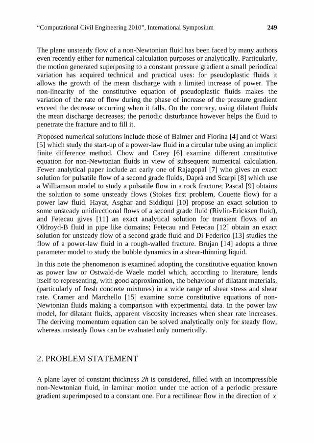
“Computational Civil Engineering 2010”, International Symposium 249
The plane unsteady flow of a non-Newtonian fluid has been faced by many authors even recently either for numerical calculation purposes or analytically. Particularly, the motion generated superposing to a constant pressure gradient a small periodical variation has acquired technical and practical uses: for pseudoplastic fluids it allows the growth of the mean discharge with a limited increase of power. The non-linearity of the constitutive equation of pseudoplastic fluids makes the variation of the rate of flow during the phase of increase of the pressure gradient exceed the decrease occurring when it falls. On the contrary, using dilatant fluids the mean discharge decreases; the periodic disturbance however helps the fluid to penetrate the fracture and to fill it.
Proposed numerical solutions include those of Balmer and Fiorina [4] and of Warsi [5] which study the start-up of a power-law fluid in a circular tube using an implicit finite difference method. Chow and Carey [6] examine different constitutive equation for non-Newtonian fluids in view of subsequent numerical calculation. Fewer analytical paper include an early one of Rajagopal [7] who gives an exact solution for pulsatile flow of a second grade fluids, Daprà and Scarpi [8] which use a Williamson model to study a pulsatile flow in a rock fracture; Pascal [9] obtains the solution to some unsteady flows (Stokes first problem, Couette flow) for a power law fluid. Hayat, Asghar and Siddiqui [10] propose an exact solution to some unsteady unidirectional flows of a second grade fluid (Rivlin-Ericksen fluid), and Fetecau gives [11] an exact analytical solution for transient flows of an Oldroyd-B fluid in pipe like domains; Fetecau and Fetecau [12] obtain an exact solution for unsteady flow of a second grade fluid and Di Federico [13] studies the flow of a power-law fluid in a rough-walled fracture. Brujan [14] adopts a three parameter model to study the bubble dynamics in a shear-thinning liquid.
In this note the phenomenon is examined adopting the constitutive equation known as power law or Ostwald-de Waele model which, according to literature, lends itself to representing, with good approximation, the behaviour of dilatant materials, (particularly of fresh concrete mixtures) in a wide range of shear stress and shear rate. Cramer and Marchello [15] examine some constitutive equations of non-Newtonian fluids making a comparison with experimental data. In the power law model, for dilatant fluids, apparent viscosity increases when shear rate increases. The deriving momentum equation can be solved analytically only for steady flow, whereas unsteady flows can be evaluated only numerically.
2. PROBLEM STATEMENT
A plane layer of constant thickness 2h is considered, filled with an incompressible non-Newtonian fluid, in laminar motion under the action of a periodic pressure gradient superimposed to a constant one. For a rectilinear flow in the direction of x

250 I. Daprà, G. Scarpi
axis, taking into account the continuity equation, the momentum equation can be written:
p u
x y t
(1)
where is the normal to the layer (y h y h ), p the pressure, the shear stress
( x y ), the velocity, u the fluid density and t the time.
If the fluid is a dilatant one, we use the Ostwald-de Waele model to describe its rheological behaviour. This model fits the experimental data of some fresh concrete; the rheological properties of fresh concrete are widely described in [16]: in what follows the yield stress is supposed to be negligible so that the shear stress can be written as
1n
du duk
dy dy
(2)
where is the shear rate, k is the consistency and the power-law index:
for dilatant fluids .
/du dy n
1n
Supposing 0 1 gp
Px
t
, where g t is a periodic function, eq. (1)
becomes
0 1 gu
P ty t
(3)
In steady flow g t 0 and eq. (3) can be solved analytically; the velocity su
which satisfies the no-slip condition at the walls is
1/
1 1/1 1/0
1
nnn
s
Pnu y h y
n k
(4)
which gives the steady discharge
1/
2 1/02
2 1
n
ns
PnQ
n k
h (5)
and the steady mean velocity
1/
1 1/0
2 1
n
ns
PnV
n k
h (6)

“Computational Civil Engineering 2010”, International Symposium 251
Introducing the following dimensionless quantities
y
h , sV
T th
, s
uw
V ,
2sV
, 0 0 2s
hP P
V ,
n
sVk
h
, the former
equations (2) and (3) become
1n
w w
(7)
and
1
0 1 Gn
w w wP T
T
(8)
where G gT t
3. NUMERICAL SOLUTION
Eq. (8) is solved numerically for two different fresh concretes, supposing
g sint t and thus G sinT T , where s
h
V (sinusoidal wave),
or
2 12
g2 1 2 1
NNt
tN N
t
i.e.
2 12
G2 1 2 1
NNT
TN N
T
where N is an integer (square wave).
The two fresh concrete used are identified in [16] as BHP9B and BHP11A respectively. The concretes are produced with gravel having maximum size of
, a coarse sand, a single-size fine sand and an ordinary portland cement (ASTM type I/II). The HRWRA (High-Range Water-Reducing Admixtures) used 12 mm

252 I. Daprà, G. Scarpi
is of the naphthalene type. The introduction of such admixtures in concrete has enhanced the durability, increased the strength, and improved the workability to levels that previously were unattainable. The physical properties are:
3
3
BHP9B 2395 kg m 1.67 92 Pa s
BHP11A 2348 kg m 1.16 217 Pa s
n
n
n k
n k
Supposing and 0.001 m 1 mmh 10 1 MPa mP ; the generalized Reynolds
number is 2
0
12 sVRe
P h
; recalling (6) it results:
5
5
BHP9B 1.61 mm/ s 7.41 10
BHP11A 1.30 mm/ s 4.79 10s
s
V Re
V Re
which ensure that the flow is always laminar . In fig. 1 the rheological behaviour of the two concrete mixtures (shear stress versus shear rate) approximated by the Ostwald-de Waele law is plotted.
0
1000
2000
3000
4000
5000
0 2 4 6 8 10
du /dy
BHP9BBHP11A
Figure 1. Shear stress (Pa) versus shear rate (s-1) for the two concrete mixtures
The discretized equation corresponding to (8) is
1
0 2
1 1 1 11 1 1 1
1 G2
2 2
jnj ji
i
j j j j j j ji i i i i i i
TP T T n
w w w w w w w w
ji
(9)

“Computational Civil Engineering 2010”, International Symposium 253
where i and j refer to space and time respectively, and 1 1
2
j jj i i
i
w w
.
The solution has been carried out with an implicit difference method, using a spatial uniform grid of 202 points (200 internal points), the adopted step was then
2 / 201 ; a finer grid does not produce appreciable effects on the results. The
time step suitable to avoid numerical instability was 710T . The numerical procedure has been tested evaluating the steady velocity profile and comparing it with the theoretical solution (4): the found differences are everywhere less than 0.8‰. Fig. 2 shows the comparison between the steady velocity profile obtained with analytical and numerical calculation and emphasizes the very strong agreement between the results of the two procedures.
0
0.2
0.4
0.6
0.8
1
0 0.5 1 1.5 2 2.5 3
u
y
analytical BHP9B
numerical BHP9B
analytical BHP11A
numerical BHP11A
Figure 2. Steady velocity profiles (mm/s); the layer thickness is 2 2 mmh
In a semi-logarithmic plot, Fig. 3 shows the mean discharge in a period as a function of the frequency of the square wave disturbance (dimensionless variables) with 0.25 . The results emphasize that the mean discharge reduces if a periodic change of pressure gradient is superimposed, owing to the non linearity of the constitutive equation of the mixture whose apparent viscosity increases with increasing shear rate ( ); the decrease does not depend on the frequency 1n f if
. A periodic disturbance however, allows a better penetration of the mixture. For very high frequencies the discharge tends to reach the steady value.
1000f
In fig. 4 the mean discharge in a period for 0 1 and for 1f Hz is plotted,
whereas fig. 5. shows the percent difference / /s s Q Q sQ Q Q of the mean
discharge in a period versus for 1f Hz. The sinusoidal pressure disturbance

254 I. Daprà, G. Scarpi
causes a percent decrease of the mean discharge which is approximately an half of the percent decrease due to the square-wave of the same amplitude.
1.98
1.984
1.988
1.992
1.996
2
0.001 0.01 0.1 1 10 100 1000 10000 100000
f
q
BHP9B
BHP11A
Figure 3. Mean discharge in a period versus frequency of the square wave disturbance; 0.25 (dimensionless quantities)
2.2
2.4
2.6
2.8
3
3.2
3.4
0 0.1 0.2 0.3 0.4 0.5 0.6 0.7 0.8 0.9 1
Q
BHP9B sq
BHP9B sinBHP11A sq
BHP11A sin
Figure 4. Mean discharge (cm3s-1m-1) in a period versus ; 1f Hz
(sq = square wave, sin = sinusoidal wave)

“Computational Civil Engineering 2010”, International Symposium 255
0%
5%
10%
15%
20%
25%
0 0.1 0.2 0.3 0.4 0.5 0.6 0.7 0.8 0.9 1
Q/Q
s
BHP9B sq
BHP9B sin
BHP11A sqBHP11A sin
Figure 5. Percent difference of mean discharge in a period versus for Hz
(sq = square wave, sin = sinusoidal wave)
1f
4. CONCLUSIONS
In this paper a numerical solution for a pulsatile flow of a non-Newtonian fluid in a fracture has been determined. An oscillating pressure gradient superimposed to a constant one allows a better penetration of the reinforcement fluid in the fracture. The rheological behaviour of the fluid is described by the Ostwald-de Waele model and the fracture has been simulated by two parallel plates. The fluids to be injected are mixtures of fresh concrete with addition of superplasticizers.
The calculation has been carried out for two dilatant fluids and for two different periodic disturbances, a sinusoidal and a square wave using an implicit finite difference method. The provided results emphasize that by pulsatile flow the mean value in a period of the rate of flow decreases, owing to the non linearity of the material. The changes of mean discharge, which are almost independent of frequency, have been calculated for different amplitude of the periodic disturbances.
References
1. Tsang, Y.W., Tsang, C.F., Channel Model of Flow through Fractured Media, Water Resources
Research, 23:467-479, 1987. 2. Neuzil, C.E., Tracy, J.V., Flow through Fractures, Water Resources Research, 17:191-199, 1981.

256 I. Daprà, G. Scarpi
3. Zimmerman, R.W., Bodvarsson, G.S., Hydraulic Conductivity of Rock Fractures, Transport in Porous Media, 23:1-30, 1996.
4. Balmer, T., Fiorina, M.A., Unsteady flow of an inelastic Power-law fluid in a circular tube, Journal of Non-Newtonian Fluid Mechanics, 7:189-198, 1980.
5. Warsi, Z.U.A., Unsteady flow of power-law fluids through circular pipes, Journal of Non-Newton Fluid Mechanics, 55:197-202, 1994.
6. Chow, S.S., Carey, G.F., Numerical approximation of generalized Newtonian fluids using Powell-Sabin-Heindl elements: I. theoretical estimates, International Journal Numerical Methods in Fluids, 41:1085-1118, 2003.
7. Rajagopal, K.R., A note on unsteady unidirectional flows of a non-Newtonian fluid, International Journal Non-Linear Mechanics, 17:369-373, 1982.
8. Daprà, I., Scarpi, G., Perturbation solution for pulsatile flow of a non-Newtonian Williamson fluid in a rock fracture, International Journal of Rock Mechanics & Mining Sciences, vol. 44, 271-278, 2007.
9. Pascal, H., Similarity solutions to some unsteady flows of non-Newtonian fluids of power law behavior, International Journal Non-Linear Mechanics, 27:759-771, 1992.
10. Hayat, T., Asghar, S., Siddiqui, A.M., Some unsteady unidirectional flows of a non-Newtonian fluid, International Journal Engineering Sciences, 38:337-346, 2000.
11. Fetecau, C., Analytical solutions for non-Newtonian fluid flows in pipe-like domains, International Journal Non-Linear Mechanics, 39:225-231, 2004.
12. Fetecau, C., Fetecau, C., Starting solution for some unsteady unidirectional flows of a second order fluid, International Journal Non-Linear Mechanics, 2005;43:781-789.
13. Di Federico, V., Estimates of Equivalent Aperture for Non-Newtonian Flow in a Rough-walled Fracture, International Journal of Rock Mechanics & Mining Sciences, 34:1133-1137, 1997.
14. Brujan, E.-A., Bubble dynamics in a compressible shear-thinning liquid, Fluid Dynamics Research, 23:291-318, 1998.
15. Cramer, S.D., Marchello, J.M., Numerical Evaluation of Models Describing Non-Newtonian Behavior, AIChE Journal, 14:980-983, 1968.
16. Garboczi, E.J., Bentz, D.P., Snyder, K.A., Martys, N.S., Stutzman, P.E., Ferraris, C.F., Bullard, J.W., Modelling and Measuring the Structure and Properties of Cement-based Materials, Electronic monograph, National Institute of Standards and Technology, Gaithersburg, 2010.

“Computational Civil Engineering 2010”, International Symposium Iasi, Romania, May 28, 2010
Practical aspects concerning nonlinear dynamic analysis
Ferencz Lazar-Mand1, Dragoş Florin Lişman2
1Dep. of Structural Mechanics, Technical Univ. of Cluj – Napoca, Cluj – Napoca, 400020, Romania 2Dep. of Structural Mechanics, Technical Univ. of Cluj – Napoca, Cluj – Napoca, 400020, Romania
Summary
The paper presents a series of aspects concerning the nonlinear dynamic analysis of pretensioned cable structures. A method for the assessment of the tangent stiffness matrix and of the nonlinear terms is proposed. The specification is similar to the one described by P. Krishna. The Newmark method is used to integrate the motion equation. In the final section of the paper a comparison between the output supplied by the software implementation of the presented method and the one supplied by DINSAS application. The elements used for comparison are the displacement and velocity response of a given pretensioned cable structures.
KEYWORDS: pretensioned, cable, nonlinear, dynamic
1. INTRODUCTION
Dynamic analysis of structures can be divided into linear and nonlinear analysis. Linear dynamic analysis can be performed on trusses and structures composed of highly pretensioned cable structures having loads that do not produce a high decrease of the pretensioning or the weakening of the cable elements. For flexible structures, a nonlinear dynamic analysis is compulsory. Mathematically, the linear behavioral model can be expressed using the following equation:
, (1) P(t)UKUCUM
,where M is the mass matrix or the inertial matrix of the system, C is the damping matrix and K is the stiffness matrix of the system [1]. All the matrices are constant. U is the node displacement vector on all the directions of the degrees of freedom,
is the node velocity vector, is the node acceleration vector and P(t) is the node equivalent forces vector. U U
Generally, for a system having n degrees of freedom, M is a symmetric and positive definite matrix of order n (diagonal for the lumped masses model), K is a
symmetric positive definite matrix of order n and the vectors , P(t) are column matrices (n x 1).
U ,U , U

258 F. Lazar-Mand, D.F. Lisman
For the nonlinear behavioral model, equation (1) can be written in a general way, namely:
, (2) P(t)U)f)UgUM ((
or
(2’) P(t)U)fU(UgUM 1 ()
where: is the damping function; Tn1nn11 )]u,,u(g)u,,u([g )Ug(
Tn1nn11 )]u,,(uf)u,,(u[ff (U)
Tn1 )]t(p)t([ptP )(
is the stiffness function and
is the excitation function.
For the linear behavioral model, the solution of the equation can be obtained either by modal analysis or through direct integration.
The solution for equation (2) is called dynamic response with displacements
U(t), with velocities and with accelerations . (t)U (t)U
If f and g are linear, equation (2) becomes linear and is equivalent to equation (1). In the Newton method (for non-linear systems), the jacobian matrix of function f can be identified. This matrix is called the tangent stiffness matrix and can be expressed the following way:
Uj
i
U
fUA
)( ;
This matrix will be presented in detail in the next chapter.
2. EVALUATION METHOD FOR A(U)
For equation (2), namely:
P(t)U)f)UgUM ((
,f(U) is considered to be:
R(U)UKf(U) (3)
,where: K is the stiffness matrix, U is the node displacement vector and R is the vector of residual terms which contains the nonlinear terms in U.
The elements of the stiffness matrix are computed using a method similar to the one in [2]. The stiffness matrix is presented for the example of a cable – beam

“Computational Civil Engineering 2010”, International Symposium 259
(6 nodes – 12 degrees of freedom), example described in [3]. This can be simply generalized for structures with 3 degrees of freedom per node.
Fig. 1
The topology of the cable – beam is described like in NELSAS [4].
The node incident elements are those elements that enter the node using edges directed towards the node. Using these node incident edges we create an array to optimally compute the structure.
The incident directed edges to a node are defined for this example in the following way: I – through the length of the cable, right direction and II – vertically descending.
The table of the node incident elements on directions I and II is:
Node incident direction Node
I II 1 9-1 1-3 0 1-2 2 10-2 2-4 1-2 0 3 1-3 3-5 0 3-4 4 2-4 4-6 3-4 0 5 3-5 5-7 0 5-6 6 4-6 6-8 5-6 0 7 5-7 0 0 0 8 6-8 0 0 0 9 0 9-1 0 0
10 0 10-2 0 0

260 F. Lazar-Mand, D.F. Lisman
The structure of the stiffness matrix is:
666564
56555453
4645444342
3534333231
24232221
131211
KKK000
KKKK00
KKKKK0
0KKKKK
00KKKK
000KKK
K
The computation of the matrix elements is performed using:
31132112
21311911
KK ;KK
;KKKK
Explicitly:
yy
31yx
31
xy31
xx31
31KK
KKK
where:
2pq2
pq2
pqpq,pq,ji,
jy
ix
ji,
iixyji,
2iyiii
ji,
yyji,
2ixiii
ji,
xxji,
zzyyxxl ll
θθl
FEAK
θFEAFl
1K
θFEAFl
1K
Obs. The “i”th element is defined by IN – FN(Initial Node – Final Node) like in [5]. In the case of spatial structures we will have the terms for the third direction,
namely “z”, too. The direction cosines: are computed using the
nodes coordinates.
z)y,x,(dθi
d
Fi – initial prestress force in a cable element i; E – modulus of elasticity; A – cross- sectional area of cable; θ – direction cosines; l –length of a cable elements .
p,q
pq
p,q
pq
p,q
pqp,q l
zz;
l
yy;
l
xx

“Computational Civil Engineering 2010”, International Symposium 261
Fig. 2 Node „q” is connected to nodes p1 – p3, using the directed edges J = 1,3
The node displacements vector is:
12
11
4
3
2
1
y6
x6
y2
x2
y1
x1
6
2
1
u
u
u
u
u
u
u
u
u
u
u
u
U
U
U
U
The residual terms vector from (3) can be expressed as:
(3’)
12
11
4
3
2
1
y6
x6
y2
x2
y1
x1
6
2
1
r
r
r
r
r
r
r
r
r
r
r
r
R
R
R
R
In node 1, on direction x:
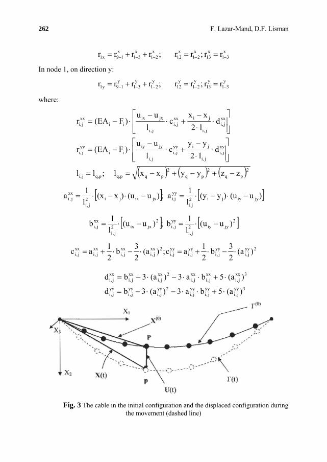
262 F. Lazar-Mand, D.F. Lisman
x31
x13
x21
x12
x21
x31
x19x1 rr ;rr ;rrrr
In node 1, on direction y:
y31
y13
y21
y12
y21
y31
y19y1 rr ;rr ;rrrr
where:
2pq2
pq2
pqpq,pq,ji,
yyj,i
j,i
jiyyj,i
j,i
jyiyii
yyji,
xxj,i
j,i
jixxj,i
j,i
jxixii
xxji,
zzyyxxl ;ll
dl2
yyc
l
uu)FEA(r
dl2
xxc
l
uu)FEA(r
)u(u)y(yl
1; a)u(u)x(x
l
1a jyiyji2
i,j
yyi,jjxixji2
j,i
xxj,i
2jyiy2
j,i
yyj,i
2jxix2
j,i
xxj,i )uu(
l
1b ;)uu(
l
1b
2yyj,i
yyj,i
yyj,i
yyj,i
2xxj,i
xxj,i
xxj,i
xxj,i )a(
2
3b
2
1ac;)a(
2
3b
2
1ac
3yy
j,iyy
j,iyy
j,i2yy
j,iyy
j,iyy
j,i
3xxj,i
xxj,i
xxj,i
2xxj,i
xxj,i
xxj,i
)a(5ba3)a(3bd
)a(5ba3)a(3bd
Fig. 3 The cable in the initial configuration and the displaced configuration during the movement (dashed line)

“Computational Civil Engineering 2010”, International Symposium 263
X = X(0) + U
X(t) = X(0) + U(t)
Configurations:
t 00 )()( - initial configuration at time t0.
t)( - configuration at time t.
Markers:
OX1X2X3 - general marker (fixed)
P Є Г(0), P(X1,X2,X3) - a generic point on Г(0).
p Є Г , p(x1,x2,x3) - position of P, at time t.
U(t) is the displacement vector from t0 to t.
{X1,X2,X3} are called material coordinates or Lagrange’s coordinates. There are the ”identifiers” of point P.
{x1,x2,x3} are called spatial coordinates.
The movement is defined by the following functions:
Xk = xk(X1X2X3,t), where k = 1,2,3
The equations above describe the material or Lagrange’s representation of movement. Using vectors the equations can be rewritten as: x = x(X, t), where X = {X1,X2,X3} and x = {x1,x2,x3}. The displacement vector is described as :
U = x – X, U = {U1,U2,U3}.
2.1 Evaluation of A(U)
In the Newton method [6], [7], [8] (for nonlinear systems) there is a tangent matrix called the jacobian matrix of function f. This matrix is:
Uj
i
U
f)U(A
After applying derivation of function f in (3) with respect to U, one obtains:

264 F. Lazar-Mand, D.F. Lisman
N
N
3
N
2
N
1
N
N
2
3
2
2
2
1
2
N
1
3
1
2
1
1
1
u
r
u
r
u
r
u
r
u
r
u
r
u
r
u
ru
r
u
r
u
r
u
r
K)U(A
where K, R and U are previously described.
3. THE NEWMARK DIRECT INTEGRATION PROCEDURE
This is one of the most used operators due to its precision and stability characteristics. The formulae for a single equation proposed by Newmark are [9]:
1i2
i2
21
ii1i uhuh)(uhuu (4)
1iii1i uhuh)1(uu (5)
In the case: 21 , the method introduces an artificial damping of the displacement
response, which is proportional to 21 . Considering 2
1 , equation (5)
becomes:
1i21
i21
i1i uhuhuu (5')
Formulae (4,5’) are controlled by parameter β. For this reason, the method is called β-Newmark method [10]. The operator is implicit because it contains in the second member. Formulae (4, 5’) can be rewritten as:
1iu
1i2
i2
21
ii1i uhuhuhuu (5a)
1iii1i uhuhuu (5b)
1ii1i uuu (5c)
where i1i1i uuu
u
represent the increase in acceleration at the end of the interval. Thus, the formulae estimate the remainder in Taylor series of the functions u and [11].
For a system, formulae (5 a-c) are:

“Computational Civil Engineering 2010”, International Symposium 265
1i1i1i UUU (6a)
1i1i1i UUU (6b)
(6c) 1ii1i UUU
,where the functions with a bar superscript represent the truncated Taylor series, namely:
1i2
21
ii1i hh UUUU (7a)
ii1i hUUU (7b)
3.1 Integration of equation (2)
In order to simplify the notation, we denote with 1 the index of the current step and with 0 the index of the previous ( 11i0i tt,tt ). By replacing (6 a, b, c) in (2),
we obtain:
)t()h()h()( 112
11110 PUUfUUgUUM (8)
and denoting:
, 1UW
equation (9) becomes:
0WF )( (9a)
Using the notations in § 2, R(U)UKf(U) . Thus we have:
)t(
)h(R)h(K)h()(
10
21
211
PUM
WUWUWUgWMWF
(9b)
Equation (9a) is solved using the Newton method or using the fixed point iteration [6]. Each integration step in the solution is performed in order to compute:
. 1i UW
3.1 Newton Method
We denote with J(W) the jacobian of function F, namely:

266 F. Lazar-Mand, D.F. Lisman
)h(AhKh)h(h)( 21R
221 WUWUBMWJ
,where B and AR are the jacobians of functions g and R. K is the stiffness matrix that appears in the formula due to the fact that during the evaluation of f‘s jacobian, terms K and R were considered. The iteration scheme is:
)F(W)δJ(W n1nn (10a)
0 W;δWW 01nn1n (10b)
Iteration (10) is considered until one of the following conditions is met: , number of iterations LNIT, where EPS and LNIT are previously
chosen. Generally, a reduced number of iterations is sufficient. ε||δ|| 1n
4. CASE STUDIES
The test structure is the cable - beam presented in the figure below [3]. Based on this structure example the stiffness matrix, displacements, etc. were computed.
Structure’s Properties
Elements IN -
FN Force .(kgf) Area (cm2) E (kgf/cm2) EA (kgf)
1 9 – 1 33.000000 0.126 2100000 263893.77 2 1 – 3 29.168200 0.126 2100000 263893.77 3 3 – 5 29.168200 0.126 2100000 263893.77 4 5 – 7 33.000000 0.126 2100000 263893.77 5 6 – 8 33.000000 0.126 2100000 263893.77 6 4 – 6 29.168200 0.126 2100000 263893.77 7 2 – 4 29.168200 0.126 2100000 263893.77 8 10 –2 33.000000 0.126 2100000 263893.77 9 1 – 2 9.904040 0.126 2100000 263893.77
10 3 – 4 14.158600 0.126 2100000 263893.77 11 5 – 6 9.904040 0.126 2100000 263893.77
The structure is composed of 10 nodes, 4 of the nodes are fixed and the geometry of the structure has the elements measured in centimeters.

“Computational Civil Engineering 2010”, International Symposium 267
Fig. 4
4.1 Mass Modeling
The system has 12 degrees of freedom (6 nodes), and M is a positive definite diagonal matrix (12 x 12), like:
6
6
2
2
1
1
m000000
0m00000
000000
000m000
0000m00
00000m0
000000m
M
where, m1, m2, ..., m6 are equal, having a 1 kg mass and are applied in the 6 “free" nodes.
4.2 Load Modeling
For this example, an impulse load is considered as dynamic load for the superior cable P0 = 10 daN (see Fig. 5).

268 F. Lazar-Mand, D.F. Lisman
This force is applied on nodes 1, 3 and 5 on the direction of y axis having the (-) sign for 0.5 seconds.
Fig. 5
4.3 Results
In the following figures we present a graphical representation of the comparison between the displacements and velocities computed using the DINSAS software application and the ones computed using our application. The displacements and the velocities are computed for node number 3 on direction y, t0 = 0 and TT = 0.5 seconds, using the step Δt = 1E-4.

“Computational Civil Engineering 2010”, International Symposium 269

270 F. Lazar-Mand, D.F. Lisman
5. CONCLUSIONS
The paper presents a method that can be used to perform nonlinear dynamic analysis of pretensioned cable structures. The method uses as starting point the equations described by P. Krishna and uses the Newmark direct integration procedure which is also described in the paper. The nonlinear terms and the tangent stiffness matrix form a function and the central study of the paper is focused on evaluating the jacobian which can be found in the integration equations.
The case study is a cable – beam which was computed and the displacement and velocities responses were graphically compared with the results computed using the DINSAS software application.
References
1. Clough, R.W., Penzien, J., Dynamics of structures, McGraw-Hill, New York, 1975. 2. Krishna, P., Cable – Suspended Roofs, McGraw-Hill Inc., 1978. 3. Volokh, K. Yu., Nonlinear analysis of underconstrained structures, International Journal of
Solids and Structures, vol. 36, 1999. 4. Chisăliţă, A., Program NELSAS – Manual de utilizare, Universitatea Tehnică din Cluj Napoca,
2007. (romanian) 5. Chisăliţă, A., Program DINSAS – Manual de utilizare, Universitatea Tehnică din Cluj Napoca, 2007. (romanian) 6. Chisăliţă, A., Numerical Analysis, Universitatea Tehnică din Cluj Napoca, 2002. 7. Trîmbiţaş, R. T., Numerical Analysis in MATLAB, Cluj University Press, 2009. 8. Coman, Gh., Numerical Analysis An Advanced Course, Cluj University Press, 2007. 9. Newmark, N. M., A Method of Computation for Structural Dynamics, ASCE Journal of the
Engineering Mechanics Division, Vol. 85 No. EM3, (1959). 10. Bathe, K. J., Finite Element Procedures, Prentice-Hall Inc., 1996. 11. Chisăliţă, A., Chisăliţă, F., Analyse de l’operateur de Newmark, Studia Univ. Babeş-Bolyai,
Mathemathica, XXXVIII, 4, 1993.

“Computational Civil Engineering 2010”, International Symposium Iasi, Romania, May 28, 2010
Structural analysis problems of complex structures
Ludovic Kopenetz1, Alexandru Cătărig1 1Department of Structural Mechanics, TechnicalUniversity, Cluj-Napoca, 400020, Romania
Summary
Complex structures have as common feature the existence of large geometric dimensions both vertically and horizontally.
These structures require special attention from the designers to meet the conditions of strength and stability in static actions and especially at dynamic actions.
Structural behavior parameters are usually: vertical and horizontal displacements, velocities, accelerations and specific deformations.
Reliability of structural analysis results in static and dynamic regime is based on the adaptation of the mathematical methods for the entire structure and correct assessment of the load assumptions.
Choosing approximated mathematical model and interpreting the results are the most difficult phases of analysis.
In this paper the authors present issues related to the required structural analysis using advanced methods of investigation and the concepts of systems theory.
KEYWORDS: ecostructures, structural materials, include energy, environment, physical element, biological element.
1. INTRODUCTION
Complex structures generally have large dimensions both vertically and horizontally.
Using this kind of constructions, as high as possible, with lateral plane or swirling surfaces, can be considered one of the important features of the development of present science and structural technique, [1], [2], [3 ].
Applying in practise of these tendencies is done according to the emergence of new structural concepts, combined with innovative structural materials and advanced specific technologies.

272 L. Kopenetz, Al. Cătărig
The complex structures recently realized are characterized by the use of certain materials having high strength and by slim, even dearing, constructive solutions.
In many cases, such constructions have significant displacements, which impact both the geometry and the sicurity of the structure, facts that might have been neglected during the designing phase.
For the new structural tendencies in the domain of the complex structures, the definition given by Architect ADA Luise HUXTABLE (USA), proves to be true: “A modern construction is that construction which could not have been built in any previous century.”
Examples illustrating this statement are many:
- The TURNING TORSO buildings in MALMO (SWEDEN), the
figure and the design CHICAGO SPIRE (Fig.1).
Figure1. Turning Torso (Malmo) and Chicago Spire
- Similar structural forms can also be found in the ABSOLUTE TOWERS 1 and 2 (Fig.2).

“Computational Civil Engineering 2010”, International Symposium 273
Figure 2. Absolute Towers
- The WEST BAY LAGOON PLAZA buildings, also known as the Dancing Towers (Fig.3).
Figure 3. Dancing Towers
- Superscraper buildings, with more than 150 stories, like the building BURJ KHALIFA over 800 m high (Fig.4). There also exists a new project called GREENWICH MERIDIAN TOWER, which will be more than 1600 m high.

274 L. Kopenetz, Al. Cătărig
Figure 4. Burj Khalifa - structures with large apertures, the so-called Pantadomes (the
stadium in SINGAPORE, ST. JORDI, FUKUI, NIMAHAYA, NARA HALL etc.) (Fig.5).
Figure 5. The Stadium in Singapore - The paper deals with the problem of the complex structures from
both the aspects concerning the conception, design and execution of these buildings and their observing the EUROCODES and the international codes.

“Computational Civil Engineering 2010”, International Symposium 275
2. NEW CONCEPTS THAT INFLUENCE THE DESIGN OF COMPLEX STRUCTURES
Keeping in mind that the construction industry has an extraordinary impact over the environment and the natural resources, it becomes clear that these aspects must occupy an important role in structural design, [4], [5], [6].
Every structure must meet the following general criteria: - to be secure, to have strength from the constructive point of
view, - to be durable, - to be aesthetic and economic. - to meet the function for which it was designed.
Besides these classical basic conditions new requirements for structural robustness are added:
- avoidance of chain or progressive collapse, due to certain local or global structural failures due to the severe wind or the shock wave given by terrorist attacks,
- keeping the structural integrity, respectively the adaptability to extremely severe actions.
Consequently, the designers face the following aspects: - usage of ecological cements, - concrete reinforced with natural and artificial fibres, - construction techniques that use the earth found in situ, - usage of thermal insulators of the aerogel type, - widening of the use of lightweight structures made of steel and
wood, - setting a number of piezoelectric systems in order to generate
power from the action of pedestrian circulation over the pavement,
- large usage of solar and photovoltaic panels.
As we can see the sustainability requirements are closely related to both the economic, robustness and security criteria and to the problems concerning the impact over the environment (natural, social and economic).
In order to best observe the sustainability of the complex structures, we strive firstly at the reduction of the quantity of structural materials used.

276 L. Kopenetz, Al. Cătărig
In this respect we promote the principle that the using the static nondetermination is always advisable. If the problems pertaining to the rigidity of the lightweight bearing structures are solved, promoting them is a favorable idea. We consider as being a universal truth the fact that braced girders are more economical than Vierendeel beams.
There still are cases when, for manufacturing reasons or other considerations, the Vierendeel beam is more advantageous for the purpose in mind, as compared to the regular braced girder.
The bearing structure from the condition for durable development must be according to the following requirements:
- quick manufacturing with reduced consumption of structural material,
- the distribution of the bearing elements must not induce functional impediments,
- assuring adeqaute natural lighting, - reduced maintenance costs.
Reducing the time needed for building has become the most relevant factor when it comes to building complex constructions.
As far as materials are concerned we can note that the basic structural materials remain the steel and the structural concrete, as the highly reliable concrete (BIR) and high performance concrete (BIP).
The question rises: when is profitable to use the concrete steel and prestressed concrete structure and when to use the steel structure? In parallel with the diversification of the technological methods and of the methods from the constructions industry a number of countries use more and more the steel structures. A few of the reasons are: - the weight of the steel structures is significantly diminished as compared to that of the structural concrete structures (using smaller hoisting equipments, quick and easy installing, easy execution of the foundation and the simple and low cost transportation in the case of terrains with reduced geotechnical size), - simple and exclusive manufacturing in industrial conditions, - in case of demolition, 100% of the material from the structure is reused as starting material, - putting up the structure and realizing large apertures is relatively easy.
The structures made in the variant of the structural concrete have the advantage of lower cost and higher resistance to fire.

“Computational Civil Engineering 2010”, International Symposium 277
3. CONCEPT AND MANUFACTURING OF COMPLEX STRUCTURES
The concept of the bearing structure is closely linked to the constructive solution which has been adopted, [7], [8]. The structural concept will seek to take over, in secure conditions, the permanent and variable loads, and especially those loads which bring about dynamic stresses (wind, earthquake). The same concept also aims at solving stable behaviour from exceptional actions (explosion, fire, shock from airplanes hitting the building as a result of human error or from a terrorist attack). In this respect, usage of a certain structure capable to avoid the chain collapse of a building is very important, even if certain structural elements or parts of the construction are accidentally destroyed, [9], [10]. The correct making of the bearing structure implies, for complex structures also, a correct fastening of the component parts to a base (foundation or another stable construction) of the ensemble of component parts, interconnected in a way to form a fixed geometric system, theoretically not movable (geometrically invariable in the view of the EUCLID model).
Avoiding the mechanism character (system or kinetic chain) of the structure is done by the appropriate setting of the necessary number of joints (equal to or higher than the number of degrees of freedom of the ensemble of component parts) both between the elements (inner joints) and between the structure and the fixing base (external joints - bearings), [11], [12], [13].
In this respect observing the natural laws is a basic condition even from the time when the structures are conceived, taking into consideration that nature strives for the equilibrium state, with the least possible investment in structural material, [14].
Professor EDUARDO TORROJA, in his paper PHILOSOPHY OF STRUCTURES, formulates this requirement like this: „We must strive for the minimal consumption of matter. Designing of structures is more than only science and technique. It has much in common with art, with realistic thinking, with endowment, with the broad line joy of creating, to which scientific calculation has the finishing touch, certifying the health of the structure and the fact that it corresponds to functioning.”
This statement is totally true, when we consider that, in so many cases, from the statical viewpoint, structures fall under precollapse or collapse state but they still stand because they are properly set up and the structural elements support each other.

278 L. Kopenetz, Al. Cătărig
Proper conception and structural set up are of essence, while the statical model and the dimensioning have a subsidiary character.
According to the opinion of a few great structuralists, it is regrettable that today we lack exactly this view. Many architects and engineers show a tendency to creat new things without taking into consideration the sustainability criteria, [15].
According to the observation of the great architect-engineer P. L. NERVI (L’architecture d’aujour’hui XII-1961): „The abundance of modalities of the structural solutions must not lead to unnatural static structures, which is structures that are born from the nonpersonal laws of static and which juggle with the forces. This represents, now, in my opinion, the worst danger for the engineering constructions”.
In this context, in order to realize structures which go along the line of durable development, choosing the engineering activity of the highest level is the best option.
Because of the multitude of parameters that must be observed, this choosing operation cannot be done automatically, even if at present there are multiple expert program systems, [16], [17].
Architects adopt different structural concepts, with many elements taken from the biostructural world, when they realize actual, modern structures.
Thus, architect SANTIAGO CALATRAVA used, for the design of the building called the TURNING TORSO from MALMO, 9 cubes (each having 6 floors) which turn, from the base of the building to its top by 90 degrees, resembling the human spine.
For the design of the CHICAGO SPIRE building, architect CALATRAVA imagined a spiral shape inspired by the shape of the rattlesnake or by the shape of a twisted tree.
In this case, each of the 150 floors turns by about 2 degrees, the last floor achieving a full rotation of 360 degrees.
Another concept can be seen in the case of high zig-zag shaped buildings, by the architect ZAHA HADID, for WEST BAY LAGOON PLAZA. These buildings, 143 m high, induced a sensation of dancing buildings, thus bringing the concept of choreographic fluidity in architecture. This way, a new class of buildings emerge, the so-called DANCING TOWERS.

“Computational Civil Engineering 2010”, International Symposium 279
The buildings ABSOLUTE TOWER 1 and 2, were named the YIN AND YANG, because of their shape. The South Tower plays the role of the woman and the North Tower, being the strong man.
A new cathegory of complex buildings called green or ecological structures, are conceived in a way that makes possible that they rotate due to the wind. The rotation can be done for one floor of for a group of floors.
Thus, a new concept emerges, that of the dynamical architecture, besides the already established structural architecture.
Analysing some complex structures that already exist, which are correctly conceived, we can see that they concur, in many respects with the requirements for durable development, existing today.
Essentially, complex structures are spatial systems having the following structural schemes:
- rigid frames in both directions, - windbracing frames in both directions, - nucleus or nuclei and peripheral poles, - tube, tube in tube, and multiple tubes.
The bearing structure is chosen according to the following considerations: - the destination of the building (offices, hotel, dwellings, etc.), - the shape, the size and the degree of occupation of the available
terrain, - the climatic and seimic zone, - the geotechnical conditions, - the financial conditions, - the structural materials and installing and execution technology; - the H/B ratio (H = height and B = the minimum plane
dimensions of the building), - the type of envelope and the kind of installations used (heating,
electricity, air conditioning, water supply, drainage, elevators, signaling, etc).
Considering that the bearing structure is worth about 10-15% of the total cost, the analysis for choosing the optimum structure is of utmost importance.
In order to be conforming with the seismic protection, when choices concerning the shape are done, the following requirements are observed:
- performing a plane symmetry, the ideal solution being a circular, square or rectangular structure,
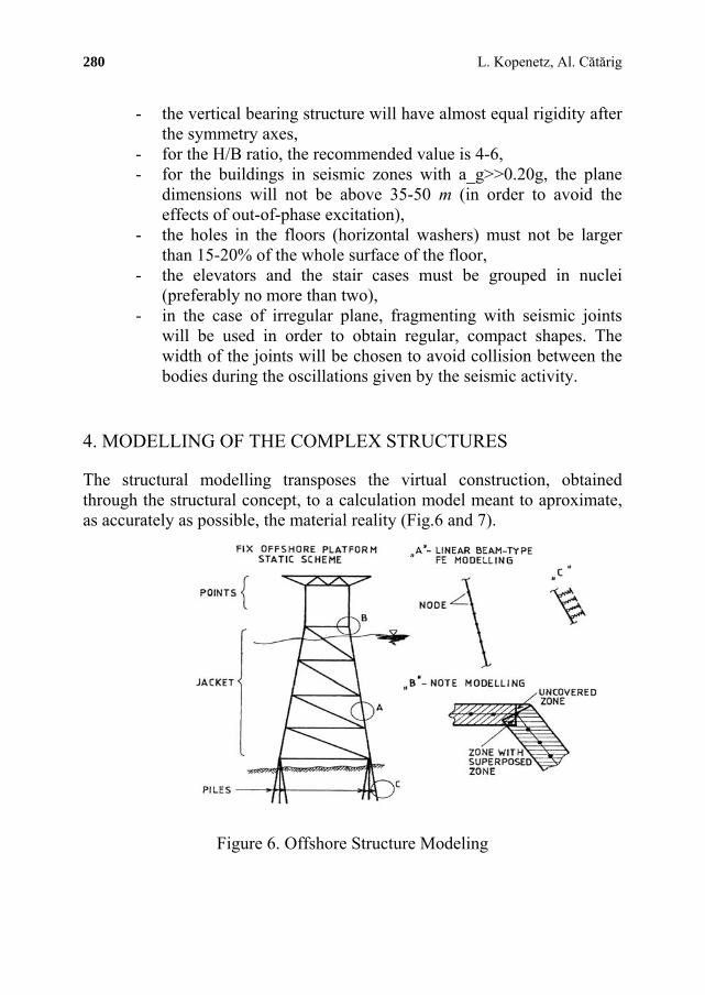
280 L. Kopenetz, Al. Cătărig
- the vertical bearing structure will have almost equal rigidity after the symmetry axes,
- for the H/B ratio, the recommended value is 4-6, - for the buildings in seismic zones with a_g>>0.20g, the plane
dimensions will not be above 35-50 m (in order to avoid the effects of out-of-phase excitation),
- the holes in the floors (horizontal washers) must not be larger than 15-20% of the whole surface of the floor,
- the elevators and the stair cases must be grouped in nuclei (preferably no more than two),
- in the case of irregular plane, fragmenting with seismic joints will be used in order to obtain regular, compact shapes. The width of the joints will be chosen to avoid collision between the bodies during the oscillations given by the seismic activity.
4. MODELLING OF THE COMPLEX STRUCTURES
The structural modelling transposes the virtual construction, obtained through the structural concept, to a calculation model meant to aproximate, as accurately as possible, the material reality (Fig.6 and 7).
Figure 6. Offshore Structure Modeling

“Computational Civil Engineering 2010”, International Symposium 281
Fig
ure
7. C
able
-sta
yed
Bri
dge
Mod
elin
g

282 L. Kopenetz, Al. Cătărig
Using the models made of bars, for the preliminary analysis, it becomes evident, as a tendency, that the analysis methods involved are simpler, more intuitive and easier to apply as compared to those referring to plates or blocks.
The simplest possible scheme will be used as the structural scheme, only this simpliifcation must not lead us to results that are diverted greatly from the real behaviour of the buildings, under different stresses.
5. ASPECTS OF STRUCTURAL ANALYSIS
It is advised to follow the next stages when we do a structural analysis: the general analysis, the preliminary analysis and the final analysis.
The general analysis must solve the following: - naming the bearing vertical subensembles, - the rational distribution of vertical and horizontal rigidity for each subenesemble, - the interaction between the vertical subensembles (frames, structural walls made of concrete and masonry).
During the preliminary analysis the following issues are solved: - the stresses and deformations are determined, for both static and dynamic regimen (plan or spatial modal analyses), - evaluation of the general torsion, - in the case of the seismic analyses, the sections having devices for dissipating of the energy will be mentioned, including the concept of their design.
The final analysis specifies the designing actions. Thus, for the seismic action the specification will according to the macro and microzoning (the free period of the terrain or the angle period) and the type of the structure.
Keeping in mind that the designing activity is 99% computer aided it is of utmost importance to control the order of magnitute of the results (Fig.8 and 9).
As it is already know, the results of a automatic calculation depend on both the physical modellation and quality of the calculation software used.
Thus, cases are know when the same complex structures were recalculated several times with the same modelling and calculation errors, due to the exactness of the mathematical apparatus implemented in the programme).

“Computational Civil Engineering 2010”, International Symposium 283
In order to eliminate this major danger and for the pre-dimensioning the structure, engineering structural analysis methods are still needed.
Figure 8. Aspects of Structural Analysis
In Europe and the U.S.A. the calculation of the complex structures is done based on the semiprobabilistic method of the limit state, which means that the structure which was conceived and executed no longer corresponds to the maximal bearing capacity and normal exploitation requirements.

284 L. Kopenetz, Al. Cătărig
Fig
ure
9. E
xem
ple
of U
sing
Mac
ro E
lem
ents
for
Str
uctu
ral A
naly
sis

“Computational Civil Engineering 2010”, International Symposium 285
For the response of large, slightly non-linear buildings, the procedure of superposing separately calculated responses is admissible, [17], [18].
In these cases, for large structures (over 6000 degrees of freedom) the RITZ reduction method may also be applied, as the method of subspatial iteration.
The way complex structures behave under the action of wind, usually differs significantly from the behavior of the common structures, due to the presence of flexibility.
In most codes, the wind action is only considered for usual constructions, for the non-usual ones special studies of wind engineering must be done.
It is known fact that at the weather stations the velocity of wind is measured with the plate weathercock, reading two values: the average velocity over two minutes’ time and the instantaneous velocity (the velocity of the gust), [19].
In the conditions found in Câmpia Română, the average velocity can be considred as being between 25 – 35 m/s. Considering the normal Gauss distribution, the ca 2% ensurace corresponds to the velocity of 35 m/s, and for 25 m/s we have 30% ensurance. For calculation, we can consider that the maximal velocity is the average velocity amplified by 1.5-1.8 (with a linear relation between the velocities).
As for the gusts, it has been statistically established that for average velocities of over 15 m/s the period of the gusts is between 1.0 and 2.0 seconds.
For severe winds, a stirring motion will be considered instead of a streamline flow. Thus, in the opinion of Professor R. H. Scanlan (U.S.A.) at the action of the gust a buffering occurs. The action of wind on the complex structures must be considered both from the static and dynamic aspects.
6. PROBLEMS PERTAINING TO MONITORING THE EXISTING COMPLEX BEARING STRUCTURES
The importance of the concepts regarding the structural robustness of the complex buildings (high buildings and buildings with large apertures) called the attention of the engineers after the terrorist attacks and after the behavior of the constructions during extreme actions (tsunami, fire, severe winds, etc.).

286 L. Kopenetz, Al. Cătărig
Monitoring the existing complex bearing structures appear as a major necessity as most of this kind of structures do not meet the structural robustness requirements.
The structural robustness level of an existing complex structure can be established based on a number of breakdown scenarios and taking into consideration the vulnerability and the effective decay degree.
Permanent or temporary monitoring should be considered in cases where major defficiencies are noticed on the structural robustness level, for the constructions in which eliminating those defficiencies would cost much and their functioning would have to be stopped temprarily.
The concept of monitoring the complex structures differs fundamentally from the concept of continuous and special observing as seen in the national code P130-99 and in similar codes from abroad.
Monitoring must be capable to detect, with reasonable costs, the following: - occurrence of structural discontinuities (holes, open or partially open joints, even breakdown in constructive joints. (Under certain conditions of catastrophic propagation can lead to the collapse of the building.), - breaking (separation) of a structural material due to current stresses, - occurrence and propagation of cracking with a certain speed.
The propagation speed of cracking depends on the internal defects (micro cracks, non-homogeneities, presence of different materials etc.) and the existence of micro defects (fractures, holes, joints etc).
Monitoring of these phenomena can be done microscopically or macroscopically.
The conception of monitoring intends to record securely the measures to be monitored and the specialness that emerges from the structural material used.
Choosing the model, the measures to be monitored, as well as interpreting the results are the most difficult phases of the structural monitoring.
Structural monitoring must be done according to the combination of the most unfavorable actions, which are possible from a practical point of view.
For the general monitoring of geometry and of primary coordinates, photogrammetry is the most advisable method.

“Computational Civil Engineering 2010”, International Symposium 287
For the structures having very large dimensions, aerial photogrammetry is advisable. For high complex structures, closed photogrammetry is enough.
7. CONCLUSIONS
- Complex structures, characterized by large dimensions (apertures, heights), require special attention on the part of the designers and those who check the projects, seeking to meet the conditions needed for strength and stability to static, and especially to dynamic actions.
- The concept “THE SKY IS THE LIMIT”, launched in the 1900s, after the first skyscraper, the HOME INSURANCE BUILDING, was built in Chicago, still applies to the present day tendency for complex structures.
- The complexity of the structural analysis for these buildings occurs as a consequence of both the large dimensions and the nonlinear behavior of these mechanical systems, with three classical sources: geometrical, physical and geometric-physical nonlinearity.
References
1. Kopenetz, L., Kollo, G., Problems of Applied Statics, International Conference of Civil Engineering and Architecture, Şumuleu (Romania), 2004.
2. Kopenetz, L., Ionescu, A., Lightweight Roof for Dwellings, International Journal for Housingand its Aplication, vol. 9, no. 3, Miami (Florida), 1985.
3. Cătărig, A., Kopenetz, L., Alexa, P., Nonlinear Analysis of Static and Dynamic Stability of Metallic Chimneys. Thin-Walled Structures, Elsevir Applied Sciences Publishers, vol.20, 1994.
4. Taranath, Y., Bungale, S., Structural Analysis and Design of Tall Buildings, Mc Graw Hill, New York, 1998.
5. Jahn, H., Genesis of a Tower, Architectural Technology, American Institute of Architecture, 1983.
6. Barratt, K., Logic and Design, Eastview Editions, Westfield, 1980. 7. Lee, L.T., Collins, J.D., Engineering Risk Management for Structures, Journal of the Structural
Division, ASCE 103, no. ST9, 1977. 8. Lanczos, K., Space Through the Ages, Academic Press Inc., London, 1970. 9. Jammer, M., Concepts of Space, Harvard University Press, Harvard, 1954. 10. Salvadori, M., Building, the Fight Against Gravity, Atheneum, New York, 1979. 11. Simu, E., Scanlan, R.H., Wind Effects on Structures, John Wiley & Sons, 1986. 12. Cătărig, A., Kopenetz, L.,Alexa, P., Problems of Stability Control of Light Structures via Active
and Passive Dampers. Proceedings of the Second International Conference on COUPLED INSTABILITIES IN METAL STRUCTURES, Liege, 1996.
13. Cătărig, A., Kopenetz, L., Alexa, P., Analysis problems of tubular offshore structures. Proceedings Seventh International Symposium on Tubular Structures, Miskolc (Hungary), 1996.
14. Kopenetz, L., Cătărig, A., Teoria structurilor uşoare cu cabluri şi membrane, Ed. U.T. PRES, Cluj-Napoca, 2006. (in Romanian)

288 L. Kopenetz, Al. Cătărig
15. Kopenetz, L., Statical Aspects and Economical Requirements of Load_Bearing Structure, International Conference of Civil Engineering and Architecture, Şumuleu (Romania), 2006.
16. Kopenetz, L., Cătărig, A., Alexa, P., Safety of Damaged Historical Building,. Local Seminar of
IASS Polish Chapter, XIII LSCE, Warsaw, 2007. 17. Ghiocel, D., Lungu, D., Wind, Snow and Temperature Effects on Structures, BasedonProbability,
Abacus Press, Turbridge Wells, Kent, U.K., 1972. 18. Lungu, D., Geldner, P., Characteristics of Wind Turbulence with Applications to Wind Codes,
2_nd European & African Conference on Wind Engineering, Genova, 1997. 19. Niemann, H.J., Modelling of Wind Loads with Regard to gust Effects, Eng. Structures, vol.6,
1984.

“Computational Civil Engineering 2010”, International Symposium Iasi, Romania, May 28, 2010
Analysis for the use of fire sand as alternative filler in the manufacture of facing tilling elements based on glass
Tomáš Melichar Faculty of civil engineering, Institute of Technology of Building Materials and Components, Brno
University of Technology, Brno, 602 00, Czech Republic, [email protected]
Summary
This article describes the possibility of waste foundry sand usage in the manufacture of facing elements based on glass is analyzed. This is just one of many possible raw materials susceptible to modify the composition of the glass facing the elements. The data presented in this article are therefore only partial chapters of extensive research which is going on VUT FAST Brno. Already several types of secondary respectively waste materials (CRT glass, container glass, flat glass, etc.) have been analyzed. For purposes of this sub-research the first sand parameters were investigated and the results have been taken on the modified batches proposal. The proposed modified formulation was used for made a few batches modified by waste materials (substitution in the range of 5 to 50 percent was considered), therefore, several sets of test specimens on which were used for the basic physical-mechanical and chemical parameters investigation. In the conclusion, the analysis results are confronted with the outputs of a previous research (concretely relating to FBC ash, finely ground blast furnace slag).
The analysis performed clearly shows the unsuitability of the selected alternative fillers, i.e., foundry sand as a replacement ingredient for sintered materials based on granular glass. Behavior of the filler at elevated temperatures, in combination with particles of glass, concrete fragments, can be compared to the pre-scanned fluid ash, which is also totally inadequate for these purposes. Simply we can say that in effect there is a loss of coherence of the charge, which can be attributed to several factors (differences in the sintering temperature – i.e., material characteristics, chemistry, etc.). For further research into the modification of materials based on sintered glass granulate, recycled foundry sand is completely unacceptable, and its utilization in building materials continue to be sought in other ways (such as alternative filler in composites with polymer matrix, scattering, etc.).
KEYWORDS: fire sand, alternative filler, facing tilling element, glass, increased temperature.

290 T. Melichar
1. INTRODUCTION
Given the current situation of production and waste management, as well as the use of secondary materials in order to limit consumption of primary sources of energy, there is a considerable variety of advanced technologies which provide some solutions to this problem. Industrial production of building materials and components is no exception. Even here it is possible through the years to observe efforts to optimize and streamline the production of many building materials. In some cases, utilization of waste in the form of secondary raw materials has reached even to the extent that these materials are used and considered as a primary source, which also reflects their availability in the market and of course, this aspect also reflects on their market price. This group of materials also derives its specific name, mainly from the way in which they are acquired, the so-called secondary energy products, such as classic high-ash, and eventually blast furnace slag. Despite the relatively numerous uses of waste and secondary raw materials fairly significant percentage of various types of waste are still being produced and hence the search for new ways and possibilities for their application. One of these is foundry sand, which arises from the forms for casting (cast steel, etc.) that have exhausted their lifetime and cannot continue to be used for further production. When considering the material characteristics of the waste material, one does not necessarily come to the conclusion that it is a valuable resource. The reason is the high percentage of silica content of fine aggregates, which is also used, for example, for glass production. Foundry sand usually contains min. 80-99% SiO2. Other supporting components are different, clay, soil (bentonite) or macromolecular substances that are the basis for connective tissue components necessary to maintain the shape of casting molds.
Given that production takes place in the casting forms at very high temperatures, chemical reactions occur in the matrix itself and thus form a certain degradation of silicate fillers such as forms for re-manufacturing or use as additives in silicate cement composites. For this reason it is necessary to look for alternative uses such as foundry sand aggregates into the matrices, which will ensure its inert behavior. Examples include composites with a polymer matrix, which provide huge potential in this context. Among the possibilities for the utilization of used foundry sand as alternative filler is the replacement of component materials based on sintered glass granulate.
2. SINTERED MATERIALS BASED ON GRANULATED GLASS
Materials based on sintered glass granulate, sometimes called Glass-silikates are a relatively new progressive material with high performance. References from

“Computational Civil Engineering 2010”, International Symposium 291
literature on these materials, offering very interesting architectural possibilities have been known for several decades. Production of these materials, particularly in the form of facing small-format elements and then elements of the façade of larger formats (or even tiles), began to boom only in recent years, when the architectural aspects of construction received more emphasis than before. To simplify, the production of glass-silicate elements can be described as thermal treatment of granulated glass, when the maximum temperature in the manufacturing process is around 1000 ° C. Although it is mainly based on the manufacturing process of glass materials, the process is rather reminiscent of technologies used to produce ceramic components. Given the purpose of the glass-silicate elements, ie, eventually a wall, tiles and their parameters are evaluated according to standards that define the basic parameters of ceramic glazed elements and wall facing. Cladding materials based on sintered glass granulate are then used due to their very good parameters in both interior and exterior of buildings. Characterized by high chemical resistance, frost resistance, colorfastness, environmental quality, and physico-mechanical properties such as flexural strength, ceramic materials are similar (about 20-30 N.mm-2), but the elastic and thermodynamic characteristics rather depend on the parameters of the type of glass. The appearance and concrete structure of these materials resemble conventional wall facing of cut stone, ie, marble, granite, etc. This characteristic is also required, and appearance is achieved by a suitable temperature regime in combination with granular enamel in specific fractions. wall Color variability based on granular glass is then ensured by adding powdered pigments, or enamel applied to the charge.
Given the dominant content of SiO2 in foundry sand, this therefore seems appropriate to modify the composition of the charge of Glass-silicates. From the above and taking into account the characteristics of foundry sand it is evident that its content will be limited. The reason is the content of impurities - bentonite, polymers, etc, cooked ingredients, casting molds, which can negatively affect the final parameters of facing elements. It is also the difference in chemical composition, which is also related to thermodynamic behavior.
3. ANALYSIS OF FOUNDRY SAND
For research purposes, it was necessary to analyze the characteristics of waste foundry sand. The results of analysis should highlight the possibility of using this material as a replacement component for the above mentioned Glass-silicate materials. For the sake of a fair assessment, all parameters in the following physicochemical analysis were performed in greater measure:
▪ chemical analysis ▪ X-ray diffraction analysis ▪ differential thermal analysis

292 T. Melichar
Further examined the characteristics of foundry sand and determination was made: ▪ particle size distribuditon ▪ specific surface area
3.1. Chemical analysis
Through chemical analysis of the contents of recycled foundry sand, the basic components were determined (alerts. FS). The results of the analysis of chemical constituents are quantified in the following table, ie, Tab. 1, which also makes comparisons with pre-researched secondary materials - fluidized bed ash (the alerts. FBC) and finely ground blast furnace slag (hereinafter alerts. FGS).
Table 1. Chemical analysis FS FBC FGS
Component Content [%]
SiO2 83.34 25.49 30.11 Al2O3 4.10 24.65 5.68 Fe2O3 2.15 7.09 1.04 CaO 0.84 22.61 37.01 MgO 0.63 0.64 6.30 Na2O 0.63 0.60 0.38 K2O 1.00 0.38 0.58 TiO2 0.43 5.35 - MnO 0.040 0.043 - Organic compounds 6.39 - - SO3 0.26 15.82 1.71 P2O5 0.08 0.32 -
Results of the chemical analysis confirmed the high silica phase, as some content alumina and ferrites, which are the basis of clay minerals, organic matter content was also quantified, which amounted to 6.39%, which is not negligible (due to production technology, sintered glass-based tiles). Other components have been reported only in small quantities ie up to 1% content. The comparison of FBC and FGS is therefore characterized by striking FS containing silicate phases.
3.2. X-ray diffraction analysis
X-ray diffraction analysis occupies an irreplaceable position in the implementation of physicochemical determination of material characteristics of building material. This is a qualitative analysis, whose main task is the identification of minerals, respectively components characterizing the material. Results of XRD analysis are shown in the picture, ie Fig 1.

“Computational Civil Engineering 2010”, International Symposium 293
Figure 1. X-Ray diffraction analysis results
According to various sources of literature and scientific studies, the addition of silica sand may be present in foundry sand, bentonite, water glass, clay, graphite, resin residues and coal dust, which are intentionally added for compaction of the system where polluting products are used in molding sand.
X-ray diffraction analysis confirmed the presence of quartz (Q - unlike FBC and FGS, there entirely in crystalline form), clay minerals (Ka - kaolinite, Di - Dickie, IA - illite, Ch - chlorite) trace amounts of feldspar (Or - orthoclase, Al - Albi, An - Anorthite) and carbon (C - carbon, G - graphite). With the letter X marked in red peaks, which was not possible to precisely define what a mineral is.
3.3. Differential thermal analysis
Differential thermal analysis is overwhelmingly used to quantify minerals and other ingredients in the physicochemical determination of material characteristics of building materials. By contrast, X-ray diffraction analysis is a quantitative analysis, whose main task is to determine the quantity of minerals respectively. Ingredients found in the X-ray analysis and chemical analysis. The assessment may also be partly to deduce the thermodynamic behavior, which is also the case in manufacturing technology, materials of glass silicates very substantially. Another undoubted advantage in comparison with X-ray analysis is the identification and

294 T. Melichar
quantification of macromolecular constituents. Differential thermal analysis results are shown in the following figure, ie Fig. 2.
? Step -5,1230 % -4,5804 mg
Step -0,1923 % -0,1720 mg
Step -4,3891 % -3,9242 mg
SP MELICH, 13.04.2010 12:57:58SP MELICH, 89,4076 mg
mg
85
86
87
88
89
min
°C100 200 300 400 500 600 700 800 900
0 10 20 30 40 50 60 70 80 90
mgmin^-10,2
min0 10 20 30 40 50 60 70 80 90
°C10
min0 10 20 30 40 50 60 70 80 90
Figure 2. Differential thermal analysis results
DTA results confirmed the presence of polymeric compounds in the analysis of the sand casting molds. Content of following components was also quantified:
- Components of clay (Kaolinite, Dickite, Illite and Chlorite) – 9.43 %, - Carbonates – 0.44 %.
It is also possible that during the beginning of the decomposition of clay there was an exothermic delay, which is characteristic for the decomposition of polymer respectively, organic compounds.
3.4. Particle size distribution and specific surface area
From the perspective of grains size, it was also necessary to determine the distribution and size of individual particles of foundry sand. In this context, specific surface was also studied. Those parameters are of particular importance because of the findings and possibly eliminate the negative effects both in the actual process (dust, workability charge) of glass silicates and also on their final parameters (decrease of mechanical properties, durability, etc.). Distribution and grain size were established on the principle of laser diffraction, the Malvern

“Computational Civil Engineering 2010”, International Symposium 295
Mastersizer 2000E device EPA5011 System is already in use. Measurement and evaluation of data are included in the figure below, i.e. Fig. 3.
Figure 3. Particle Distribution Analysis
The analysis of particle size distribution shows that we’re talking about relatively soft granules with a specific surface of 87.5 m2.kg-1, compared to cement binder which is characterized by a range of 300-400 m2.kg-1. Given that the facing elements, respectively based on sintered glass granulate are generally used fractions 1-4mm with a maximum of 6 mm can be considered only a partial substitution of charge. Alternatively, it would be possible to modify the parameters of the final paving elements (eg, roughened surface layer and thus improve the slip resistance floor).
4. LABORATORY FIRING - MANUFACTURING TEST SAMPLES
With regard to the analysis, foundry sand was approached to design recipes for facing the elements based on sintered glass granulate. In the initial phase of the proposed modified formula was based purely on glass and foundry sand. Selection of pigments and other additives (the primary charge), which only modify some parameters of glass silicates to eliminate potential adverse interactions between these components and used foundry sand, which could be due to elevated

296 T. Melichar
temperatures. As reference material Borosilicate glass was chosen with a mass of 0-6 mm, which is used for production of facing and paving elements of sintered glass granulate. The composition of each batch of test formulations is shown in the following figure, ie Fig 4.
Figure 4. Composition of trial batches
System (refractory) form-batch was subsequently exposed to elevated temperatures. The maximum temperature in isothermal holding time was 900 ° C, with temperature rise and cooling phases are carried out according to a precisely defined temperature regime.
Figure 5, 6. Borosilicate granulated glass (left - Fig. 5.) and fire sand (right - Fig. 6.)

“Computational Civil Engineering 2010”, International Symposium 297
The following pictures (photographs) the structure of produced samples are recorded in detail, see Fig 5's 11th.
R02-10 R01-05
R03
-15
R04
-20
R05-35R06-50
Figure 7. View of the test specimens in refractory form (recipe markings correspond with the titles given in Figure 4)
From the photographs presented on Fig 7 it is evident that all of the proposed formulae, which were part of the substituted foundry sand charge are unsuitable, or this is an erroneous use of foundry sand for the production of sintered granular materials based on glass. The cause is probably the different sintering temperature, which in the case of enamel range from 900-960 ˚ C. By contrast, for foundry sand with a dominant content of silica sand, the temperature is almost twice as high. Another reason, which has a striking effect on the enamel-compaction of foundry sand could be found in the content of impurities arising from degradation of casting molds, ie, during the manufacturing process of steel casting. Specifically, the content of organic compounds, clay minerals, and trace amounts of carbon and graphite. It is also likely that some of the impurities contained in the foundry sand at elevated temperatures, chemically react with each other, where the enamel in the product increases the maximum isothermal holding time required for sufficient compaction of the produced sample structures.
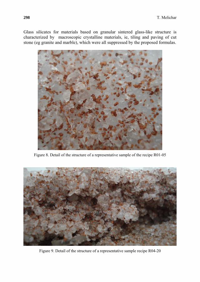
298 T. Melichar
Glass silicates for materials based on granular sintered glass-like structure is characterized by macroscopic crystalline materials, ie, tiling and paving of cut stone (eg granite and marble), which were all suppressed by the proposed formulas.
Figure 8. Detail of the structure of a representative sample of the recipe R01-05
Figure 9. Detail of the structure of a representative sample recipe R04-20

“Computational Civil Engineering 2010”, International Symposium 299
When comparing pictures of foundry sand before and after firing it is also clear that the color change, ie black (coal dust, etc.) to red, was probably caused by the firing of clay materials.
3. CONCLUSIONS
In this paper, the possibility of using foundry sand which has exhausted its useful life was described and analyzed. Specifically, the use of foundry sand as a replacement component element, on the basis of sintered glass granulate, was analyzed. Based on the analysis of physicochemical parameters and particle size distribution of alternative materials, the proposal for a recipe with a modified composition of the charge was addressed.
Results of the laboratory experiments, when foundry sand was administered at a dose of replacement glass 5-50% by weight, clearly pointed to the unsuitability of alternative fillers under existing conditions of the manufacturing process. Correction of these conditions, ie, modifying the temperature regime, possibly through the use of different additives, the production of materials capable of competition could be achieved, but this would lead to an increase in economic performance, and probably also the need to adjust the production line.
Based on previously performed experiments it can be concluded that foundry sand has a negative influence on the final parameters of glass silicate elements, similar to that of fluidized ash (FBC) and even in doses as small as the substitution of 5% charge. The best parameters were achieved when using finely ground granulated slag (FGS).
Figure 10,. Detail of the structure of a representative sample FGS01-05

300 T. Melichar
Figure 11. Detail of the structure of a representative sample FBC01-05
Acknowledgements
This result was realized with financial support from the state budget through the Ministry of Industry and Trade under the project FT-TA5/147 „Sintered products made of by-products for creation of walls and floor surface treatment" and then in the research project MSM 0021630511 „Progressive Building Materials with Utilization of Secondary Raw Materials and their Impact on Structures Durability”.
References
1. MATOUŠEK, J. Anorganické nekovové materiály, VŠCHT v Praze, 1992. 2. FANDERLIK, I. Vlastnosti skel, INFORMATORIUM Praha, 1996. 3. PYTLÍK, P.; SOKOLÁŘ, R.: Stavební keramika, technologie, vlastnosti a využití, Akademické
nakladatelství CERM, s.r.o., Brno, 2002. 4. BODNÁROVÁ, L. Kompozitní materiály ve stavebnictví, Akademické nakladatelství CERM,
s.r.o. Brno, 2002.
Appendix
This article describes the analyzed possibility of using waste foundry sand in the manufacture of facing elements based on glass. This is just one of many possible raw materials susceptible to modify the composition of the glass facing the elements.

“Computational Civil Engineering 2010”, International Symposium Iasi, Romania, May 28, 2010
Ultrasonic impulse method in parameters investigation of glass board composites
Tomáš Melichar1, David Procházka2 and Jiří Bydžovský3 1Faculty of civil engineering, Institute of Technology of Building Materials and Components, Brno
University of Technology, Brno, 602 00, Czech Republic, [email protected] 2Faculty of civil engineering, Institute of Technology of Building Materials and Components, Brno
University of Technology, Brno, 602 00, Czech Republic, [email protected] 3Faculty of civil engineering, Institute of Technology of Building Materials and Components, Brno
University of Technology, Brno, 602 00, Czech Republic, [email protected]
Summary
In this article the possibility of ultrasonic impulse method usage for physical and basic mechanical properties of composites based on glass is analyzed. Given that it is still not much explored area the paper is mainly of the retrieval character. For the glass itself, was carried out a certain number of research studies and found some results, but the board materials based on sintered glass yet devoid of any methodology for the investigation of parameters of non-destructive way. Significant is also the fact that the considered composites contain fillers alternative both amorphous and crystalline based as well. For this reason, the term glass-silicate is often used, but it is not material based on the glass ceramic matrix.
Within the framework of this research, it has been found that the assessment of physical and mechanical parameters of board glass-based composite materials is possible and that it offers certain advantages and new findings, in the scientific light as well as in terms of effective practical use.
KEYWORDS: Ultrasonic impulse method, glass composite, material science.
1. INTRODUCTION
Use of the ultrasonic impulse methods in construction practice is fairly well known and it need not be emphasized in connection with the investigation of characteristics and parameters of concrete structures. Generally, ultrasonic impulse method is, in principle, based on mechanical wave propagation in materials. It is used mainly for determining the quality of test environment, such as the uniformity of product, or its physical and mechanical characteristics based on the velocity of ultrasonic wave propagation. The principle of the ultrasonic method is that repeated electrical impulses create thin bunches of attenuated mechanical oscillation in the exciter. These mechanical impulses are then allowed to enter the test element or

302 T. Melichar, D. Procházka, J. Bydžovský
material and, after travelling the measured path L (typically of the length, width or thickness of the test samples or structural unit), are recorded by a sensor. The resulting determined parameter is the passage time of ultrasonic waves, i.e. the time t from sending the impulse by an exciter to recording its impact on the sensor. With the specified passage time and length, which ultrasonic waves have travelled, and the already mentioned propagation velocity of ultrasonic waves can be determined. In case of concrete, the ultrasonic impulse method can be used to establish or to assess, for example, a dynamic modulus of elasticity, compression strength, or uniformity. Given that concrete is a relatively heterogeneous material and the results of the ultrasonic measurements are affected by many different factors, there is a number of calibration relations, where various regression coefficients determined by the method of the smallest squares are involved, for determining a given characteristic. These calibration relations are, as is the case of Schmidt impact hammers, quite different. The following can be mentioned as disturbing and distorting elements when using the ultrasonic impulse method: reinforcement, gravel nests, cracks, and also varying elasticity or the size of the material individual components. Despite these negative factors that may affect the progress and results is using the ultrasonic impulse method convenient in terms of non-destructive nature of testing and, complying with all procedures and principles, relatively satisfactory results can be achieved that can be used to assess the basic parameters of the given material on test samples as well as in structures directly.
2. GLASS BOARD COMPOSITES
Glass in the classic sense, as it is known not only by professionals but also by general public, is described in detail in numerous publications and several studies. Using glass as a building material is an integral part of the vast majority of construction works. Board elements based on heat-treated glass granules are a relatively new and progressive building material. They rather resemble classic ground-stone tiles. However, it is an amorphous material whose batch is composed of borosilicate glass of specific fractions with the addition of tiny quantities of colouring pigments or other, parameters modifying, admixtures. Presently, the Institute of Technology of Building Materials and Components, Brno University of Technology, Brno, carries out a research into batch substitution using secondary raw materials in its entirety. The results obtained so far can be regarded as successful and beneficial, see [3], [4], [5], [6] and [7].
Testing of the basic physical and mechanical parameters of board glass-based materials depends on their current use in practice, i.e. as tiles and paving or illuminated facade elements etc. With regard to the existing normative documents, the range of ČSN EN ISO 10545-XX is used. The reason can also be found in the lack of standards related directly to materials based on sintered glass. The

“Computational Civil Engineering 2010”, International Symposium 303
determination of, e.g. bend strength, is performed using classical destructive ways, but it is necessary to prepare test samples of a corresponding format that are usually much smaller than the usual format used in structures. The advantage of using the ultrasonic impulse method for the evaluation of basic physical and mechanical characteristics (bend strength, modulus of elasticity and uniformity of material relating primarily to homogeneity, etc.) is the application on elements coming directly from a production line, which would lead to the verification of these parameters. In practice, therefore, the quality of board glass-based materials could be verified relatively easily and quickly in combination with computers containing software with calibration relations, which would certainly contribute to improving the quality of dispatched product range. Compared with concrete, sintered glass elements are materials exhibiting a relatively much higher homogeneity, which, to some extent, eliminates the adverse effects in force during the use of the ultrasonic impulse method. It is therefore advisable to consider the application of ultrasonic methods of investigation in the case of board glass-based composites and to compare the results with conventional glass, especially because of the determination and comparison of possible deviations in the diversity of these materials.
2. ULTRASONIC IMPULSE METOD AND AMORPHOUS MATERIALS
The fact that the ultrasonic impulse method can be used successfully for analyzing both the physical-mechanical and chemical properties of various glasses is confirmed by many studies that describe the basic and expanded research in this area. Many authors also focus on the evaluation of such parameters as, for example, the course of some chemical and thermodynamic processes and actions that are the consequences of either given material properties or they result from technologies of manufacturing process procedures. The study [1] presents valuable knowledge on the investigation of ultrasonic velocity and attenuation in Pb-phosphate glasses at a frequency of 10 MHz and in the temperature range of 80-300 K. The results presented here indicate clearly an indirect relationship between ultrasonic velocity and temperature. The presented relationships can be seen from the graphical interpretation (see Figures 1 and 2.).
On the other hand, scientists in [2] describe the use of ultrasonic measurements for the study of borosilicate glasses doped with selected transition metal oxides (NiO, V2O5, Fe2O3, MnO2, TiO2, Cr2O3, CoO, CuO). Their analyses were carried out under normal environment conditions (i.e. at room temperature) using the frequency of 4 MHz. Basic physical and mechanical characteristics, such as density, modulus of elasticity, Poisson coefficient, was investigated. The conclusion presents the relationships of these found analyzed parameters; the

304 T. Melichar, D. Procházka, J. Bydžovský
measured values show certain relationships that are mainly related to a particular transition metal oxide.
Figures 1 and 2. The graphs show the curves of determined ultrasonic velocities in the longitudinal direction (left - Figure 1) and right (right - Figure 2). The differences between the individual samples (i.e. Samples 1 to 6) are given by molecular ratios of the PbO and
P2O5 components. [1]
In [8], tellurite glasses of the system (100−x)TeO2–xBaO for different compositions of BaO (x=9, 12, 15, 18, 20 and 22 wt.%) have been prepared by rapid quenching method. A decrease in ultrasonic velocities and density, which is followed by an increase in attenuation with a progressive increase in BaO content has been observed at room temperature and also over a wide range of temperatures. The above results reveal the softening of the glass network due to the progressive transformation of the rigid framework characteristics of TeO2 resulting in the formation of distorted TeO3+1 units followed by the creation of regular TeO2 (4→3+1→3) sites and the formation of ionic character bond (NBO). [8]
The ultrasonic velocities (both longitudinal and shear) and attenuation measurements were carried out using a high power ultrasonic pulser–receiver system (Fallon Ultrasonics Inc. Ltd., Model: FU1050, Canada) with 100 MHz digital storage oscilloscope (Hewlett-Packard, Model: 54600 B, US) and a computer employing cross-correlation technique. 8027) and Scanning Electron Microscopy (SEM) studies (Hitachi, Model: 415A) have been made in all the

“Computational Civil Engineering 2010”, International Symposium 305
glasses to confirm the amorphous nature. The thermal behaviour of all BAT glass samples has been studied from the differential thermal analysis (DTA). [8]
Figure 3, 4. Dependence of a) longitudinal (UL) and b) shear velocity (US) in (100−x) TeO2–xBaO glasses with change in temperature for different BaO contents (Fig. 3.),
Dependence of a) bulk (K) and b) Young's modulus (Y) in (100−x)TeO2– xBaO glasses with change in temperature for different BaO contents (Fig. 4.). [8]
The transition of the progressive rigid framework characteristic of TeO2 to regular TeO3 units and ionic character bonds (NBO) is responsible for the continuous decrease in sound velocity. On the other hand, the attenuation shows an opposite behaviour to that of velocity. The softening of the network contributes to a gradual increase in the attenuation of ultrasonic waves. The temperature dependence of velocities, elastic moduli and attenuation explores more information about the structural changes and stability of the glass network. A gradual decrease (Fig. 3) in ultrasonic velocity and elastic moduli (Fig. 4) with an increase in temperature from 303 to 500 K in all BaO contents has been noticed without showing any anomaly unlike other glasses like (CuO)x–(TeO2)1−x. The formation of distorted TeO3+1 units followed by the creation of regular TeO3 (4→3+1→3) sites and the formation of ionic character bond lead to a monotonic decrease in density, ultrasonic velocity and elastic moduli, and an increase in attenuation with addition of BaO content. The temperature dependence of ultrasonic parameters reveals the structural softening in the network without showing any anomalous behaviour over a wide

306 T. Melichar, D. Procházka, J. Bydžovský
range of temperatures. The above results reveal the softening of the glass network with an increase in BaO content. [8]
In industrial thermal tempering of glass, the knowledge of the homogeneity of compressive residual stress field on the glass product is fundamental to guarantee the quality of the tempered glass product. In this paper [9], authors use the acoustoelasticity phenomenon in order to estimate the residual stress distribution by using acoustic surface wave. They present an experimental setup based on a double interferometric detection in which an aspheric lens is associated with a beam splitter and a YAG laser whose power is 100 mW. This relative high power enables us to carry out measurements on surface flat glass although optical reflection coefficient is typically weak (< 10%). Using these two points of detection, the evolution of relative surface wave velocity is obtained with a good accuracy. At last, a comparison between the numerical modelling and experimental results shows the potentiality of an ultrasonic method to estimate stress distribution in flat glass tempering. [9]
Figure 5, 6. Distribution of the Von Mises residual surface stresses in the tempered glass sample (Pa) – Fig. 5 (on left). Ultrasonic measurement and modelling of evolution of the
stress TYY along the line of coordinate y = 0 mm – Fig. 6 (on right). [9]
A flat glass (20 mm × 20 mm × 6 mm) sample has been tempered in vertical position on a laboratory tempering installation. After a first heating in a furnace, the sample moves by vertical translation to enter the zone between two nozzles. In consequence, the finite element model is limited to one eighth of the real sample (in Fig. 5., only the half thickness of the glass is considered for the modeling). Fig. 5. shows the non uniform distribution of the Von Mises residual surface stresses in the glass sample after the tempering. The distribution is non uniform with a maximum 88 MPa value in the centre of the sample. It corresponds to the maximum heat exchange. The numerical modeling gives us the two stresses along the two directions X and Y at each point of the glass sample. In order to compare the evolution of the numerical graph with the experimental graph, authors take a reference corresponding to the stress at the origin O(x = 0,y = 0) (Fig. 6). The comparison is quite encouraging: they notice that, for the measurements, the most

“Computational Civil Engineering 2010”, International Symposium 307
stressed zone is also located in the centre of the sample where the heat exchange is maximum. There is a good correlation between ultrasonic experimental and modelling.
The study [9] shows that the original double interferometric detection proposed here, is well adapted to the estimation of stresses in glass and is an alternative to the actual optical methods.
Figure 7. (a) Variation of ultrasonic attenuation coefficient with temperature of 10% PbO of
TeO2–WO3–PbO ternary glass system. (b) Variation of ultrasonic attenuation coefficient with temperature of 12.5% PbO of TeO2–WO3–PbO ternary glass system. (c) Variation of
ultrasonic attenuation coefficient with temperature of 15% PbO of TeO2–WO3–PbO ternary glass system. (d) Variation of ultrasonic attenuation coefficient with temperature of 17.5%
PbO of TeO2–WO3–PbO ternary glass system. (e) Variation of ultrasonic attenuation coefficient with temperature of 20% PbO of TeO2–WO3–PbO ternary glass system. [10]
308 T. Melichar, D. Procházka, J. Bydžovský
An ultrasonic study [10] of heavy metal tungsten tellurite glasses containing different concentration of lead oxide at different frequencies and temperatures has revealed that the ultrasonic attenuation coefficient and the internal friction show behaviour mainly determined by mechanisms having localized motions of atoms groups. Peak losses and peak temperatures are strongly affected by change of concentration and frequency, exhibiting, strong dependence on the kind and concentration of the modifier. The acoustic activation energy has been calculated and found to decrease with increasing lead oxide content. The relaxation strength, deformation potential, number of loss centres and density of state are calculated and tabulated. Both the number of loss centres and their activation energy decrease with the atomic ring size. The density of state, the deformation potential and relaxation strength are strongly dependent on α/f, especially at temperature below the peak temperature. Finally a decrease in the density of state reflects the fact that the contribution of nonbridging oxygen atoms among the particles could not be considered in this kind of study. [10]
3. CONCLUSIONS
Given the above theoretical and research-based knowledge, it can be stated clearly that the use of the ultrasonic impulse method for evaluating the parameters of board materials based on sintered-glass granulate is possible, and it can already be expected, to some extent, that it will be advantageous from several different perspectives. The advantages lie mainly in speed (assuming the creation of proper calibration relations and their definition using computer technology) and in the implementation of this non-destructive method (the determination of basic physical and mechanical characteristics – modulus of elasticity in compression, shear, bend strength, uniformity, etc.) directly in a factory producing these elements. Another significant finding is the possibility of using an appropriate methodology for the determination of residual stresses in these elements, i.e. the stress originating in the production technology and that can have a negative impact in the application of such elements in structures. Standardly, methods based on optical principle are used for glass, but study [9] presents basic knowledge and principles of residual stress evaluation on a different principle that does not require optical methods. This finding is very useful because, in case of sintered-glass granulate materials, these optical methods cannot be implemented due to the distinctive texture of such materials reminding of rock crystal panels (marble or granite).
Acknowledgements
This result has been realized with financial support from the state budget through the Ministry of Industry and Trade within the framework of project FT-TA5/147

“Computational Civil Engineering 2010”, International Symposium 309
“Sintered products made of by-products for creation of walls and floor surface treatment” and, furthermore, this contribution has been realized within the framework of specific university research project at the Brno University of Technology, No. FAST-J-11-14 “The aspects of sintered glass-based materials using waste and secondary raw materials”.
References
1. Paul, A.; Ghosh, U., S.; Basu, C.: Ultrasonic velocity and attenuation in Pb-phosphate glass, Journal of Non-Crystalline Solids 221, ELSEVIER, 1997, p. 265 - 273. URL: <www.sciencedirect.com>
2. Marzouk, S., Y.; Gaarad, M., S.: Ultrasonic study on some borosilicate glasses doped with different transition metal oxides, Solid State Communications 144, 2007, p. 478 - 483. URL: <www.sciencedirect.com>
3. Melichar, T. Využitelnost sklosilikátových desek jako součásti podlahových systémů. In Konference podlahy PODLAHY 2008. Praha, Masarykova kolej ČVUT. 2008. p. 227 - 230. ISBN 978-80-254-2560-2.
4. Melichar, T.; Bydžovský, J. Vliv přídavku druhotných surovin přidávaných při výrobě sintrovaných prvků na jejich výsledné vlastnosti. In Konference ZKOUŠENÍ A JAKOST VE STAVEBNICTVÍ 2008. Praha, Masarykova kolej ČVUT. 2008. p. 203 - 209. ISBN 978-80-01-04123-9.
5. Melichar, T.; Bydžovský, J. Úspory primárních surovin a energetických zdrojů v oblasti výroby sklosilikátových materiálů. In Proceedings of the International Conference, 15th Construmat 2009. Praha, České vysoké učení technické v Praze. 2009. p. 207 - 212. ISBN 978-80-01-04355-4
6. Melichar, T.; Bydžovský, J. Netradiční dlažby na bázi skla se zvýšeným obsahem druhotných surovin. In PODLAHY 2009. Praha, BETONCONSULT, s.r.o. 2009. p. 229 - 234. ISBN 978-80-254-5231-8.
7. Melichar, T.; Bydžovský, J. Sintrované desky na bázi skla ve stavebnictví. In SANACE A REKONSTRUKCE STAVEB 2009 31. konference. Praha, Vědecko technická společnost pro sanace staveb a péči o památky - WTA CZ. 2009. p. 226 - 231. ISBN 978-80-02-02190-2.
8. Nishara Begum, A.; Rajedran, V. Structure investigation of TeO2–BaO glass employing ultrasonic study, materials Letters 61, 2007, p. 2143 – 2146. URL: <www.sciencedirect.com>
9. Devos, D.; Duquennoy, M.; Roméo, E.; Jenot, F.; Lochegnies, D.; Ouaftouh, M.; Ourak. M. Ultrasonic evaluation of residual stresses in flat glass tempering by an original double interferometric detection, Ultrasonics 44, 2006, p. 923 - 927. URL: <www.sciencedirect.com>
10. Afifi, H.; Marzouk, S.; Abd el Aal, N. Ultrasonic characterization of heavy metal TeO2–WO3–PbO glasses below room temperature, Physica B 390, 2007, p. 65 – 70. URL: <www.sciencedirect.com>
Appendix
In this article the possibility of ultrasonic impulse method usage for physical and basic mechanical properties of composites based on glass is analyzed. Given that it is still not much explored area the paper is mainly of the retrieval character. For the glass itself, was carried out a certain number of research studies and found some results, but the sheet materials based on sintered glass yet devoid of any methodology for the investigation of parameters of non-destructive way.

“Computational Civil Engineering 2010”, International Symposium Iasi, Romania, May 28, 2010
Necessary emergency shelters after natural disasters
Oana Stanila1, George Taranu2, Razvan Sencu3, Alexandru Stanila1 and Magda Brosteanu1
1Department of Civil and Industrial Engineering, Faculty of Civil Engineering and Building Services,
“Gheorghe Asachi” Technical University of Iasi, 700050, Romania 2Department of Structural mechanics, Faculty of Civil Engineering and Building Services,
“Gheorghe Asachi” Technical University of Iasi, 700050, Romania 3 Faculty of Civil Engineering and Building Services, “Gheorghe Asachi” Technical University of
Iasi, 700050, Romania
Summary
Natural disasters occur all over the world and they influence both people and constructions. These are the effect of a natural hazard (e.g. flood, tornado, volcano eruption, earthquake, or landslide) that affects the environment, and leads to financial, environmental and/or human losses. The resulting loss depends on the capacity of the population to support or resist the disaster, and their resilience. In all of these cases, people are left without a shelter. In order to give medical assistance or to provide living spaces quickly shelters are needed.
This current paper presents the concept of a hemispheric structure which can be building at the lowest possible cost, and in a very short time, in two basic steps. The first step, after which the dome is habitable, can be finalized in six hours. The second step, also the final one, takes at most four days. The Savior Passive Hemisphere is a more suitable choice than the traditional tent method due to its passive thermal character, its capacity to be turned into a permanent construction, and its strength characteristics due to geometric shape. The main objective of this structure is to ensure an emergency shelter for the Red Cross and other intervention teams, a refuge for the people left homeless. In addition, the aspect of creating temporary shelters which can be then transformed into permanent dwellings is considered.
The behavior of this solution had been simulated in a FEM analysis, when subjected to standard environmental loading conditions prescribed by the European design codes. As a conclusion for this paper, the obtained results were compared to the strength of materials in terms of allowable stresses, deflections and displacements, in all loading combinations.
KEYWORDS: FEM analysis, emergency shelters, thermal efficiency, structural behavior

“Computational Civil Engineering 2010”, International Symposium 311
1. INTRODUCTION
Watching the horrible consequences of natural disasters, our research group strived for a solution of well insulated shelters for temporary, if not permanent, dwellings, clinics, and social buildings that could be faster built than usual, and at a lowest possible cost. The current report presents the analytical tools that our team has used for testing the temporary shelter dome shaped construction. This shelter purpose is to help the survivors of any possible tremendous earthquake based disaster.
The Emergency Shelter is basically a savior Passive Hemisphere which is a more suitable choice than the traditional tent method due to its passive character, its capacity to be turned into a permanent construction, and its strength and mechanical characteristics. The main aim of this type of structure is to help the disaster stricken people, to offer an emergency shelter for the medical assistance or to be an dwelling temporary or permanently for people remain homeless (fig. 1). In other conditions this structure can be used like mountain dwelling or holyday house (fig. 2).
Fig. 1 Emergency situation when shelters are needed
Fig. 2 Different types of use of structure

312 O. Stanila, G. Taranu, R. Sencu
2. STRUCTURE DESCRIPTION
The dome has an outer diameter of 12 meters and attains 6 meters in altitude. The solution may also have an inside wood or steel structure forming a potential first floor slab. This structure will be considered detachable from the actual dome structure and will be computed in a simple manner.
The dome walls are made by rigid polyurethane foam as structural material. The dome surface is made of a special tarpaulin material which plays an essential role against UV radiation, environmental moisture content, rain fall, or frost exposure. Basic constituents are: tarpaulins, rigid polyurethane foam, light joinery.
Fig. 3 Perspective view of the structure
3. TECHNICAL SOLUTION
The main purpose for this project was the fast construction of the structure. Following this initial idea, the technological steps that were designed are wanted to be fast and efficient ones:
Minimum arrangement of the terrain; dispose of leaves, scrubs, boulders, stones, and any possible discontinuities.

“Computational Civil Engineering 2010”, International Symposium 313
Board diaphragm mounting on the ground soil; this diaphragm is made of a rubbery tarpaulin which is highly resistant to tension and piercing. It has a protective role against water infiltrations, and it also takes over the pushing stresses.
Assembly of each slice of dome element; one constitutive element is practically a pneumatic mat of hemisphere sector shape, with several sealed compartments. Each of these compartments is provided with adjustable pressure valves.
Hemi- sphere anchorage to the soil; this step consists in the disposing on the dome contour of the anchorages, represented by helical metallic rods.
Fixing the dome; this procedure involves the fitting of the hemisphere on the vertical joints by using Velcro connections and special longitudinally hemi-flexible fasten elements. These elements are shaped as a quadrant plate and are fixed using the gilled margins of the vertical joints of the prefabricated element. Then, the horizontal cables are installed in a circular shape at the dome base line and at each horizontal datum deck level of the hemisphere elements, according to the project.
Pneumatic inflating of the dome; it is realized using compressed air, starting from the base level, and moving up, compartment by compartment, and element by element.
Doors and windows installation; the joinery, made of a light, shatterproof material, are provided with natural ventilation vents.
Air lock mounting; from this point forward, the Savior Passive Hemi- sphere is usable, having a minimum thermal resistance ensured by the air trapped in between the membrane walls.
Injection of polyurethane foam; each element is filled from bottom to top. Every sealed compartment is provided with two valves: an infusion one, at the inferior side, and a pressing one, at the superior part.
The structure is demountable and fully recoverable; by removing the quadrant plates and dismounting the hemisphere sectors the dome can be taken and repositioned on a new site, having different and variable functions.

314 O. Stanila, G. Taranu, R. Sencu
Fig. 4 Dome elements: 1-floor membrane;2-stainless steel helical anchorage; 3-inflated
base ring; 4-entrance hall; 5- quadrant plates; 6-CFRP tie rod; 7-velcro; 8- rigid polyurethane foam; 9-window system; 10-top connection element.
In Figure 2 there are presented the constitutive details of the dome and the final view of the hemisphere is shown in Figure 1.
4. DESIGN CRITERIA
The considered design criteria contain:
safety,
aesthetical shape,
fast construction,
low energy consumption,
low cost of construction,
efficient use of energy and materials,
simple technology.
The Savior Passive Hemisphere answers to these criteria by offering a functional flexibility, a simple and attractive shape, a fast construction time, and a high thermal resistance of the envelope while being suitable for almost all types of soil

“Computational Civil Engineering 2010”, International Symposium 315
footings. The final product was desired to be best from the economical and technological processes points of view. In addition, its simple construction does not require specially trained workers, making it best suited for crisis moments.
5. ELEMENTS AND MATERIALS
The considered structural elements and their materials are presented in the Table 2 [1], [2]:
Table 2. Structural element materials Structural elements Materials Dome walls Rigid polyurethane foam Covering sheet Waterproof tarp Circular reinforcement Carbon fiber reinforced polymer tape Foundation footing Reinforced concrete Inside floor structure Wood/steel work
5.1. Structural walls made by rigid polyurethane foam
Energy efficiency: polyurethane foams have one of the highest insulating R-values per mm of all commercially available products today, making it possible or the constructions to have thinner walls and lower profile roofs and still maximizing the efficiency and utilized space while reducing operating costs... When placing reflective plastic coverings over polyurethane foam-insulated roofs, they bounce the sunlight and radiant heat away from the building, helping the structure to stay cool and reducing the energy consumption for air conditioning [9].
High performance: they are strong, light weighted, dimensionally stable, moisture-resistant with very low vapor transmission, and having a very low density [10].
Easily applied: they can be sprayed on various surfaces, or molded to special shapes in relatively large sizes. They can also be protected against UV degradation.
Versatility: due to their insulating performance. Some rigid polyurethane foam can be applied in situ to seal voids and cover irregular shapes. In-situ foams are mainly used for technical insulation applications, forming a seamless structure.
Thermal and mechanical performance: they ensure a reduced energy transfer, do not deform or distort, and are not damageable by moisture that

316 O. Stanila, G. Taranu, R. Sencu
may result from condensation. These foams compressive and shear mechanical strengths are remarkable. This unique combination of properties allows rigid polyurethane foams to be used in diverse applications E.g., the foam can hold together many of the components in a refrigerator or hot-water heater while it continues to act as thermal insulation.
The environmental benefits are significant, including the increased energy efficiency and reductions in energy-efficient construction costs, reduced project weight, and savings of all other construction components that this material replaces. Better insulation results in lower energy use, the inner space can be increased due to the downsized mechanical heating and cooling equipment, thinner walls, and shorter fasteners roofs. This simple light-weighted product implies less manufacturing steps, less energy in manufacturing, and transportation.
Rigid polyurethane foam has an useful life beyond 50 years.
In conclusion, the stainable development with rigid polyurethane foam contains these aspects:
Reducing energy consumption and emissions,
Hygienic use,
Life-cycle analysis of rigid polyurethane foam,
Energy balance,
Rigid polyurethane foam - material recycling and energy recovery.
5.2. Waterproof, UV protection tarpaulin
Tarps, short for tarpaulins, are resilient, long lasting products made from a strong, water resistant and waterproof polyethylene material. They are generally used to keep things dry and free from dirt and grease, the covers are crafted from a very high- grade material, complete with a UV inhibitor, which increases the duration of the tarp even under heavy exposure to the sun [10].
Because poly tarps are generally the first choice in situations where a flexible, water resistant cover is needed, they became the perfect option for the Savior Passive Hemi-sphere external cover.
5.3. CFRP tape confinement
CFRP tapes are fast and easily installed, on any weather conditions, highly resistant and have been used with success in strengthening works. Their mechanical and

“Computational Civil Engineering 2010”, International Symposium 317
physical properties support a good behaviour and their width of 16 mm ensures that the failure of the rigid polyurethane foam will not occur [11].
5.4. Anchorage system
The anchorage system consists in fixing the horizontal membrane, which plays the floor role, with helical metallic rods, at a depth of 100 cm. These rods are made of galvanized steel, being protected against corrosion. The mounting is done by rotating these rods with a torsion moment applied at their end until they reach the desired depth.
6. NUMERICAL ANALYSIS
A finite element model had been developed to obtain the expected maximum stresses and the behaviour of the final dome structure under the load combinations detailed in section 7.2.
The used software is named AXIS VM version 9, and it had the capability of computing a wide range of stresses and forces and the program also provides the stress diagrams in the shape of coloured maps. AxisVM is a finite-element program for the static, vibration, and buckling analysis of structures. It was developed by and especially for civil engineers. Axis VM combines powerful analysis capabilities with an easy to use graphical user interface [8].
The selected structural model was appropriate for predicting the structural behaviour with an acceptable level of accuracy. The structural model was also appropriate to the limit states considered. All of these features allowed us to obtain a comprehensive analysis for the structure. The type of finite element used was shell [3], [4].
6.1. Structure loading
The expected loads to which the structure is or may be subjected are [5]:
self- weight (permanent loading)
weight from snow accumulation (variable load)
wind force upon the lateral surfaces of the dome (variable load)
seismic load (extraordinary events)
Note: The live loads are neglected as the internal floor is considered independent from the dome structure and the roof is not circulated [7].

318 O. Stanila, G. Taranu, R. Sencu
6.1.1. Snow loading
According to EN 1991-1-3, the standard recognized by the European Community, and considering any possible unfavourable location, this dome was designed to withstand a snow loading of 2,5 KN/m2.
Section 5 from EN 1991 part 1-3 shows the methods of choosing the snow loading coefficients and the subjected area for curved roofs.
6.1.2. Wind loading
The symmetry of the structure implies that the wind can blow from any direction and the dome will have practically equivalent results.
In addition, it is obvious that this special shape behaves best when subjected to wind action because of its curved roof and of its base section – altitude variation. The dome is designed to withstand a wind pressure of 0.7 kPa. This assessment is based on EN 1991-1-4. In figure 4 is presented the wind action on shell roof structures.
Wind pressure
Fig. 5 Wind pressure action [5]
6.1.3. Seismic loading
This dome is designed for the Romanian seismic region according to P100-1/2006, having the following characteristics [6]:
ag = 0.20g - peak ground acceleration
Tc=0.7 s – vibration period of control
q=1 - behaviour factor
γI =1 - importance factor for ordinary buildings
The seismic design has been performed after the vibration analysis. The seismic parameters used in software design are presented in Table 6.

“Computational Civil Engineering 2010”, International Symposium 319
Table 6. Seismic Parameters
Parameters
Reduction factor: ν = 0,5 Displacement amplification factor: c = 1 Parametric shape Importance factor: γI = 1 Ground type: Tc = 0.7 Design ground acceleration: ag = 1,916 m/s2 Behaviour factor: q = 1 Beginning of the constants section of the spectrum: TB = 0,070 s End of the constant section of the spectrum: TC = 0,700 s Beginning of the constant displacement section of the spectrum: TD = 3,000 s
Spectrum (horizontal)
Spectral value of the horizontal ground acceleration factor: �0 = 2,75 Combination of modal responses: Auto Viscous damping: ξ ’ = 0,05
Combination methods
Combination of the components of seismic action: SRSS
Table 7. Results of a vibration analysis (mode shapes and frequencies) Mode number
f [Hz] T [s] ω [rad/s] EV
1 3,96 0,252 24,89 619,35 2 3,96 0,252 24,89 619,35 3 4,75 0,210 29,87 892,01 4 5,57 0,180 34,98 1223,88 5 5,57 0,180 34,98 1223,88 6 5,70 0,175 35,84 1284,23 7 5,70 0,175 35,84 1284,23 8 6,06 0,165 38,10 1451,32 9 6,42 0,156 40,33 1626,16
Where: f - the frequency ω - the circular frequency T - the period Ev - the eigenvalue

320 O. Stanila, G. Taranu, R. Sencu
Fig. 6 Vibration Mode 1 (3.96 Hz), eY, map of displacements
7.2. Load combinations
According to EN 1990:2002, the design is limited to ultimate (ULS) and serviceability limit state (SLS) verifications of structures subject to static loading, including cases where the dynamic effects are assessed using equivalent quasi-static loads and dynamic amplification factors, including wind or traffic loads.
The structure must be designed and executed in such a way that it will, during its intended life, with appropriate degrees of reliability and in an economical way, sustain all actions and influences likely to occur during execution and use, and remain fit for the use for which it is required.
In addition, the structure must be designed to have adequate:
structural resistance,
serviceability,
durability.
In the case of fire, the structural resistance shall be adequate for the required period of time according to EN 1991-1-1-2.
6.2.1. Design situations
The selected design situations are sufficiently severe and varied so as to encompass all conditions that can reasonably be foreseen to occur during the execution and use of the structure.

“Computational Civil Engineering 2010”, International Symposium 321
A. Ultimate limit states (ULS)
These limit states concern of the safety of people and the safety of the structure.
States prior to structural collapse, which, for simplicity, are considered in place of the collapse itself, may be treated as ultimate limit states. The following ultimate limit states are to be verified when they are relevant:
loss of equilibrium of the structure or any part of it, considered as a rigid body,
failure by excessive deformation,
transformation of the structure or any part of it into a mechanism,
rupture,
loss of stability of the structure or any part of it, including supports and foundations.
A.1. Combinations of actions for persistent or transient design situations (fundamental combinations)
The general format of effects of actions is :
( , ) ( ,1) (0, ) ( , )1 2
1.35 1.5 1.5k j k i k ij j
G Q Q
Where:
Gk,j - Characteristic value of permanent action j
Qk,I - Characteristic value of the accompanying variable action i
Qk,1 - Characteristic value of the leading variable action 1
ψ0 - Factor for combination value of a variable action, ψ0=0.7
A.2. Combinations of actions for accidental design situations
The general format of effects of actions is:
( , ) ( ) (2, ) ( , )1 1
k j I Ek i k ij i
G A Q
Where:

322 O. Stanila, G. Taranu, R. Sencu
AEk - Characteristic value of seismic action (national seismic standard P100/1-2006)
γI- Importance factor (national seismic standard P100/1-2006)
Gk,j - Characteristic value of permanent action j
Qk,I - Characteristic value of the accompanying variable action i
B. Serviceability limit states (SLS)
These are the limit states that concern the functioning of the structure or structural members under normal use, the comfort of people, and the appearance of the construction works.
The verification of serviceability limit states is based on criteria concerning following aspects:
deformations that affect
the appearance,
the comfort of users,
the functioning of the structure.
vibrations that
cause discomfort to people,
limit the functional effectiveness of the structure.
damage that is likely to adversely affect
the appearance,
the durability,
the functioning of the structure.
B1. Characteristic combination:
This combination can be expressed as:
( , ) ,1) (0, ) ( , )1 2
k j k i k ij j
G Q Q
For the SPHS-sphere structural modeling there where used the Romanian national annexes of EN in the following actions and load combinations where considered:

“Computational Civil Engineering 2010”, International Symposium 323
Table.8 Load Cases
Name Group
Dead static Snow static Wind static SM + SEISM SM - SEISM
Table.9 Load Combinations
Nr. Name Dead Snow Wind SM + SM -
1 Co #1 (modal analysis) 1,00 0,40 0,40 0 0 2 Co #2 (fundamental 1) - ULS 1,35 1,50 1,05 0 0 3 Co #3 (fundamental 2) - ULS 1,35 1,05 1,50 0 0 4 Co #4 (seismic) - ULS 1,00 0,40 0,40 1,00 0 5 Co #5 (seismic) - ULS 1,00 0,40 0,40 0 1,00 6 Co #6 (characteristic 1) - SLS 1,00 1,00 0,70 0,00 0 7 Co #7 (characteristic 2) - SLS 1,00 0,70 1,00 0 0,00
6.3. Material properties
Rigid polyurethane foam: PUF 10pcf
Density: = 157,7 [kg/m3]
Compressive strength: fc = 13,8 [daN/cm2]
Poisson ratio: ν=0.001
Elastic modulus: E= 4,1368 *107 [N/m2]
6.4. Structural analysis results
The internal forces and the positive sign conventions of each surface element type are summarized in the table below.
Principal actions - n1, n2, m1, m2, represent the principal internal forces and moments. The sign conventions are as follows: m1≥m2, n1≥n2, -90<α≤ +90 (relative to the local x axis).

324 O. Stanila, G. Taranu, R. Sencu
Table.10 Calculus relations Finite element type - Shell Surface forces
Membrane Plate
n1 2
21 2 2
x y x yxy
n n n nn n
n2 2
22 2 2
x y x yxy
n n n nn n
m1 2
21 2 2
x y x yxy
m m m mm m
m2
Table 11.Surface Forces [Linear, Envelope Min, Max] Node min.
max. Case n1
[N/mm] n2 [N/mm]
m1 [daNm/m]
m2 [daNm/m]
4246 min Co #2 - ULS (f1) -18,7 -18,9 -10,9 -11,8 3327 max Co #4 - ULS (A) 17,1 -8,3 25,7 6,0 124 min Co #2 - ULS (f1) -1,5 -38,7 -0,8 -20,1 313 max Co #4 - ULS (A) 15,9 -7,4 38,9 2,5 4405 min Co #5 - ULS (A) -8,7 -17,8 -13,8 -17,1 4007 max Co #2 - ULS (f1) 11,2 -16,3 51,0 4,7 447 min Co #5 - ULS (A) -8,7 -17,9 -8,9 -24,5 2281 max Co #4 - ULS (A) 11,5 -9,1 42,8 6,9
Fig. 7 Co #2 - ULS, membrane forces n1 Fig.8 Co #2 - ULS, membrane forces n2

“Computational Civil Engineering 2010”, International Symposium 325
Fig. 9 Co #2 - ULS, moments m1 Fig.10 Co #2 - ULS, moments m2
Fig. 11 Co #2 - ULS, maximum principal stresses S1 top layer
Fig.12 Co #2 - ULS, minimum principal stresses S2 top layer
Fig. 13 Co #4 - ULS, maximum principal stresses S1 top layer
Fig.14 Co #2 - ULS, minimum principal stresses S2 top layer

326 O. Stanila, G. Taranu, R. Sencu
Table 12.Surface Stresses [Linear, Envelope Min,Max]
Node min. max.
Case Surface Pos. S1 [N/mm2]
S2 [N/mm2]
202 min Co #2 - ULS (f1) Sh 153 T -0,072 -0,073 2895 max Co #4 - ULS (A) Sh 2783 T 0,064 -0,005 124 min Co #2 - ULS (f1) Sh 84 T -0,005 -0,142
Fig. 15 Co #4 - ULS, maximum principal stresses S1 top layer
Fig.16 Co #2 - ULS, minimum principal stresses S2 top layer
Table 13. Nodal Displacements [Linear, Co #7 - SLS (c2-wind)]
Node eX [mm]
eY [mm]
eZ [mm]
57 -4,090 0,494 -1,052
2896 4,090 0,494 -1,052
1261 -0,681 -2,127 -1,035 4186 0,208 4,423 -1,117 21 0,133 0,974 -15,548 6571 0 0 -0,001
Table 14.Nodal Displacements [Linear, Co #6 - SLS (c1-snow)]
Node eX [mm]
eY [mm]
eZ [mm]
57 -4,502 0,426 -1,131 2896 4,502 0,426 -1,131 8293 -0,175 -3,104 -1,169 8463 0,175 -3,104 -1,169 13734 0,226 4,741 -1,295 21 0,159 0,675 -17,955

“Computational Civil Engineering 2010”, International Symposium 327
Table 15.Nodal Displacements [Linear, Co #4 - ULS (A)]
Node eX [mm]
eY [mm]
eZ [mm]
22 0 0,001 0 36 11,809 9,365 -7,493 1425 0,001 0 0 1474 8,788 12,301 -7,093 124 10,191 10,492 -13,263 1425 0,001 0 0
Fig. 17 Co #4 - ULS, horizontal displacements ex
Fig.18 Co #6 - SLS, horizontal displacements ex
6.5. Structural analysis conclusions
From the numerical analysis, in terms of ULS design method, the maximum tensile principal stresses, have reached the maximum value of 0.064 N/mm2, in the case of the seismic load combination; the maximum compression stresses have the value of 0.072 N/mm2, in the fundamental case combination. In addition, the minimum principal stresses in the compression are of 0.142 N/mm2, by fundamental load combination. These attained results are within the allowable limits of the considered structural material. The obtained maximum vertical displacements, in SLS design method, taken from the load combination number 6, where the snow loading is preponderant, are of 17.95 mm. Meanwhile, on the horizontal direction, the displacements have reached the value of 4.5 mm.
7. CONCLUSIONS
The primary aim of this project was to offer a temporary shelter to the survivors of tremendous disasters, like in the case of the earthquake which had happened in

328 O. Stanila, G. Taranu, R. Sencu
Haiti, not long ago. Watching the horrible consequences of natural disasters, our research group strived for a solution of well insulated shelters for temporary, if not permanent, shelters that could be built faster than usual and at a low cost.
In combination with other natural phenomena such as a frost winter or a torrid summer, the Savoir Passive Hemisphere can offer so much needed help due to its variable applicability; it can be a clinic, a multi-families house, a canteen, or a storage place. In a more optimistic manner, it could be a library, a hostel, a small concert hall, a conference or office space, or even a students’ club.
From the results of the FEM Analysis meaning the recorded stresses and displacements, the unit stresses are 88% smaller than the material strengths. This fact proves that the structure is stiff, stable, and it satisfies all considered structural performance and design criteria. From the structural point of view, the construction can be optimized by adopting a material with low mechanical strengths. A major advantage of the provided solution is the dome shape with curved surfaces inwards that consistently helping the stability and bearing capacity of the structure.
In addition, the high thermal resistance provided by the structural material gives our dome the much desired ”passive house” character by reducing the annual energy consumption and the environmental pollution.
It is our strong believe that the solution brought by The Savoir Passive Hemisphere can save many lives in the case of a future disaster.
References
1. Maji, Schreyer, Zuo, Donald and Satpathi, Mechanical Behaviour of Polyurethane Foam Impact-Limiters, ASCE J. of EMD, April, 1995, pp. 528-540.
2. Singh, D., Chen, N., Pagilla, K., Study on Degradation of a Commercial Rigid Polyurethane Foam, August 2006.
3. Mkrtchyan, L., Maier, M., Huber, U., Structural polyurethane foam: testing and modelling for automotive , Germany, 10 march 2008, International Journal of Crashworthiness, 1754-2111, Volume 13, Issue 5, 2008, Pages 523 – 532
4. Kleser, J., Technical properties of polyurethane rigid foam as an insulating material in construction. Technical Information No. 14/2000, Bayer AG
5. Euro code 1 - EN 1991 parts 1-3, 1-4; 6. P100-1/2006 The Romanian Standard For Design Of Structures For Earthquake Resistance; 7. Rogers, G., J., Report Of Structural Evaluation - Montgomery Hill Observatory, Evergreen
Valley College San Jose, California (September 6, 2002) 8. AXIS VM version 9 9. www.polyurethane.org 10. http://www.pu-europe.eu 11. http://hughesbros.com/Aslan500/Aslan500_CFRP_Tape.html

“Computational Civil Engineering 2010”, International Symposium Iasi, Romania, May 28, 2010
An efficient way of improving the safety of reinforced concrete frame structures against impact loading
Oana Mihaela Ioniţă1, Nicolae Ţăranu2 and Mihai Budescu3 1Department of Civil and Industrial Engineering, "Gh.Asachi" T.U. of Iasi, Iasi, 700050, Romania 2Department of Civil and Industrial Engineering, "Gh.Asachi" T.U. of Iasi, Iasi, 700050, Romania
3Department of Structural Mechanics, "Gh.Asachi" T.U. of Iasi, Iasi, 700050, Romania
Summary
This paper provides initially an overview of some general issues associated with the robustness of structures. Firstly, a brief discussion related to the progressive collapse, from its basic definition, to the difficulties of understanding, analysing and mitigating this phenomenon is presented. Attention is also drawn to the potential sources of abnormal loads that should be examined when designing for progressive collapse performance. In addition, some of the design standards that have been developed, and methods for designing to progressive collapse hazards are discussed.
A numerical analysis of a four storey reinforced concrete frame structure has been carried out and the results concerning the assessment of a progressively damaged structure are presented.
KEYWORDS: abnormal loads, progressive collapse, structural safety, robustness of structures, composite steel-concrete columns.
1. INTRODUCTION
The improvement in structural analysis and knowledge of the material properties over the last decades has led engineers to build structures that are structurally more efficient than in the past. This leads increasingly to exploiting the constituent materials to the limit of their operational envelope. The result is that modern structures do not have the strength reserve that was inherent in older structures engineered by empirical knowledge and instinct, and hence more attention must be given to the way in which they will perform when subjected to abnormal loads [1].
One of the main aims of modern structural design is to provide safety of structures, i.e. to reduce the risk for the humans’ life. In traditional design this objective is achieved by designing structural components against specified limit states. However, as showed the Ronan Point collapse in UK in 1968, when a gas explosion in one of flats on the 18-th floor of a 22-storey residential building caused the failure of an entire section of the building [2], this approach is not sufficient. The approach does not exclude the risk of local damage to a structure

330 O.M. Ioniţă, N. Ţăranu, M. Budescu
due to accidental events (e.g. gas or bomb explosion, vehicle impact, gross errors in design, construction and/or utilization) that may occur during service life of the structure. While probability of occurrence of such events for ordinary structures is low, and therefore, they are not considered explicitly in design, their effect on structural safety becomes significant if the structure is not robust. That happens when some local damage can trigger a chain reaction of failures causing the collapse of the whole structure or of a major part of it, the so called progressive collapse [3]. One of the structural properties that can prevent the collapse of an entire structure when only parts of it are damaged or entirely destroyed is the structural robustness. As it can be easily understood, a robust structure is also a collapse resistant one.
The progressive collapse phenomenon has been of interest to structural engineers for several decades. After the 1995 bombing of the Alfred P. Murrah Federal Building in Oklahoma City, the bombing of the US Embassies in Nairobi and Dar-Es-Salaam in 1998, and the collapse of the World Trade Center Towers in New York and a portion of the Pentagon in Washington due to the terrorist attack on September 11, 2001, the subject gained renewed interest from planners, officials, and the public at large. Lessons learnt from these events were that special attention must be given to the behavior of the structural elements to improve their redundancy, toughness and ductility under extreme events [4].
The structural engineering community has tried to address the subject of progressive collapse from many perspectives, in an effort to develop a universal approach for the evaluation and the approaching of such an event. The inherent difficulty in developing a universal approach is that the response of each structure to specific events may be different, from the initial cause of the collapse to the way that the collapse progresses throughout the structure. This irregular behavior separates progressive collapse from other well-defined structural engineering problems such as wind, seismic load, and vibration [5].
The consequences of the progressive collapse can adequately be economically quantified, but more important, unfortunately, they can be sometimes quantified in lost lives. That is why it is of a great importance for structural engineers to develop methods for preventing and mitigating the progressive collapse of structures, enabling people to safely evacuate the affected buildings in the event of such a disaster [5].
The ultimate goal of the protection against progressive collapse is to minimize injuries and loss of lives and to facilitate the evacuation and rescue of survivors. The casualties that will occur to occupants in the immediate vicinity of the explosion or impact may be unavoidable, but by preventing progressive collapse, the remaining occupants may be safe from injury or death [4].

“Computational Civil Engineering 2010”, International Symposium 331
2. PROBLEM STATEMENT. KEY ISSUES
Progressive collapse is a catastrophic partial or total structural failure arising from an event that causes local damage that cannot be absorbed by the inherent continuity and ductility of the structural system [9]. The residual structure is forced to seek alternative load paths in order to redistribute the loads applied to it. As a result, the other elements may fail causing further load redistribution. This process might continue until the structure can find equilibrium by finding stable alternative load paths [6]. Therefore, a local damage or failure initiates a chain reaction of failures that propagates vertically or horizontally through the structural system, leading to an extensive partial or total collapse. While virtually all structural collapses initiate from a local damage, it is generally agreed that the key feature distinguishing progressive collapse is that the resulting damage is disproportionate to the local damage caused by the initiating event. Such collapses can be initiated by many causes, including abnormal loads not normally considered in design (e.g. gas explosions, vehicular collisions, and sabotage), severe fires, extreme environmental effects that stress the building system well beyond the design envelope, human errors in design and construction, and misuse. All buildings are susceptible to progressive collapse in varying degrees [7, 8].
Specific design approaches to prevent progressive collapse as a result of abnormal loads have not been standardized. There are a number of reference papers on the subject and some studies leading to techniques that can be employed economically for certain construction types. However, building codes and standards that address the issue invariably treat general structural integrity and progressive collapse in qualitative rather than quantitative terms. This is due, in part, to the elusive nature of the definition of general structural integrity and the countless ways by which resistance to progressive collapse can be achieved. Moreover, the lack of quantitative provisions results from the difficulty that the engineering profession has encountered in defining specific events or initial conditions for which progressive collapse resistance should be considered, or the tolerable damage state of a building system that has restrained a progressive collapse successfully. Finally, there is the question of what the acceptable risk is? No building system can be engineered and constructed to be absolutely risk-free in the presence of numerous sources of uncertainties that arise in the building process or from potential failure-initiating events. Building codes and standards provide tools for structural engineers to manage risk in the public interest. Of course, code provisions address the risks in building performance as the code and standard-writers have understood and confronted them at particular points in time. The renewed interest in abnormal loads, progressive collapse, and the associated hazards and risks is now taking place in a context that is very different from that historical understanding. Provisions for progressive collapse-resistant design have yet to be identified in terms of either performance level or risk [9].

332 O.M. Ioniţă, N. Ţăranu, M. Budescu
3. METHODOLOGY
Current efforts are aimed at the development of explicit design methods for reducing the potential of progressive collapse for new and existing structures, too.
The abnormal loading on structures is not limited to high-rise buildings only. It has to be taken into account when designing any kind of structures. Abnormal load events may arise from various sources: gas explosion, confined dust or vapour conflagration, machine malfunction, bombs, high explosive effects, vehicle, aircraft or missile impact etc. [1].
A progressive collapse event is defined by ASCE 7-05 as “the spread of an initial local failure from element to element, eventually resulting in the collapse of the entire structure or a disproportionately large part of it” [10].
This definition of progressive collapse provides the first indication on how to approach a progressive collapse analysis. Certainly, the first step in evaluating the progressive collapse potential in a structure is to determine whether the initial target structural element, typically a column, has failed. In some cases, the target element is assumed to fail. The next step is to determine whether this failure has spread to adjacent elements, including beams, columns, and connections. Ultimately, the structural engineer must determine how much of the structure is expected to fail as a result of the structural member that was lost initially (Figure 1) [5].
a) intact structure b) initial loss of a column and
subsequent failures in the floors above
c) failures propagating to the other bays
Figure 1. Phases of progressive collapse
4. EVALUATION METHODS
Current design standards that address progressive collapse design issues include those of the General Services Administration (GSA) and the Unified Facilities Criteria (UFC) adopted by the Department of Defense (DoD). These standards

“Computational Civil Engineering 2010”, International Symposium 333
provide two means of assessing progressive collapse in the design of new buildings or the evaluation of existing ones [5].
The GSA Progressive Collapse Analysis and Design Guidelines have adopted the Alternate Path approach to address progressive collapse issues. By adopting this methodology, the designer is required to systematically remove key gravity load carrying elements (columns or load-bearing walls) around the perimeter of the building and design the remaining structure to redistribute the loads without collapse. For a regular structure, a minimum of three separate analyses is required to adequately satisfy the criteria.
A ground floor perimeter column, or a portion of the ground floor load-bearing wall, must be removed at the following three locations: middle of the long side of the building, middle of the short side of the building, and a corner location. For irregular structures, such as those containing reentrant corners, soft stories, closely spaced columns, or transfer girders, additional analyses may be required to adequately address all conditions [11].
The Unified Facilities Criteria document, UFC 4-023-03: Design of Buildings to Resist Progressive Collapse outlines four different levels of protection, ranging from Very Low Level of Protection (VLLOP) to High Level of Protection (HLOP), and the corresponding progressive collapse design requirements. For the Very Low and Low Levels of Protection, the UFC allows for the use of tie forces in resisting progressive collapse.
The tie force methodology, which is generally consistent with the design standards of the United Kingdom, is threat independent and is intended to provide a minimum level of “fault tolerance” without consideration of specific failure mechanisms.
The UFC document defines peripheral, internal, vertical, and horizontal tie forces that must be developed through the structural connections and sufficiently anchored at the member ends. This will effectively “tie” the structure together and allow for the redistribution of loads following local damage. The tie force methodology relies on catenary action, rather than flexural response, and therefore a structure designed in this manner will generally develop larger deformations following the loss of an element than a structure designed using the Alternate Path approach. For the Medium and High Protection Levels, an Alternate Path analysis is required, in lieu of prescribing tie forces [12].
According to UFC document, in the case of buildings where the public access is restricted, the most critical locations for removing external columns are the following ones: near the middle of the short side, near the middle of the long side, and at the corner of the building, as shown in Figure 2 [12].

334 O.M. Ioniţă, N. Ţăranu, M. Budescu
SIMILAR SHORT SIDE COLUMNS
COLUMN REMOVAL
LOCATIONS
SIM
ILA
R L
ON
G
SID
E C
OLU
MN
S
PLAN VIEW Figure 2. Locations of external column removal [12]
In the case of structures with underground parking or other areas of uncontrolled public access, the most critical locations for removing internal columns are the following ones: near the middle of the short side, near the middle of the long side and at the corner of the uncontrolled space, as shown in Figure 3. The removed column extends from the floor of the underground parking area or uncontrolled public floor area to the next floor (i.e. one story height must be removed) [12].
PLAN VIEW
SIM
ILA
R L
ON
G
SID
E C
OL
UM
NS
SIMILAR SHORT SIDE COLUMNS
INTERIOR COLUMN
REMOVAL LOCATIONS
PUBLIC ACCESS SPACES
(HATCHED AREA)
Figure 3. Locations of internal column removal [12]

“Computational Civil Engineering 2010”, International Symposium 335
5. ANALYSIS, PREVENTION AND MITIGATION
There have been many cases in history that have highlighted the dangers associated with the progressive collapse of a building. Recent events have underlined the importance of taking extreme events into consideration in the design of a structure. While it is not practical to retrofit every building in the world to resist every possible threat scenario, it is important to understand how existing structures will respond to these events. The goal is to limit the loss of human life and the extent of localized damage. In addition, it is necessary to ensure the safety of rescue personnel so that they can enter buildings safely and reach the survivors in the event of a disaster [5].
It is the responsibility of the structural engineer to come up with practical design solutions for mitigating progressive collapse damage. Engineers must have an understanding of the fundamental response of the structures that they are designing, so that they can develop solutions that can be implemented without raising the costs of a project to astronomical levels [5].
Finally, when a disaster does occur, it is necessary to have a rapid means of assessing the safety and stability of the structure. Development of fast-running software tools allows rescue crews to determine whether a building is safe enough to enter, and whether a building is in danger of imminent collapse. These tools can also be used as a rapid assessment tool in the design phase of a project, allowing engineers to get a sense of the structural response to a particular threat scenario [5].
6. CASE STUDIES
A simple four storey reinforced concrete framing system was analysed in this study. The plan view and structural configuration of the analysed structure are shown in Figure 4. As it is shown in the figure, the structure consists of two spans and three bays each of them of 6.00m. The story height is 3.00m. The perimeter and central columns are spaced at 6.00m.

336 O.M. Ioniţă, N. Ţăranu, M. Budescu
a) 3D view b) plan view
damaged columns
Figure 4. Structural configuration
The load bearing system of the structure consists of reinforced concrete columns, beams and slabs. The structural members’ properties are indicated in the following table:
Table 1 Structural members’ properties Structural member Width
[cm] Height [cm]
Concrete class
Columns 55.00 55.00 C25/30 Beams 30.00 60.00 C25/30 Slabs - 15.00 C25/30
The structural modelling has been carried out using the Autodesk Robot Structural Analysis 2010 software.
For the purpose of this study, in addition to the permanent loads of the structure (i.e. dead loads (DL) of the structural elements), the following loading conditions have been assumed: the snow load (SN) at the terrace level of 2kN/m2 and a live load (LL) on each level of 2kN/m2. The following two load combinations have been considered: 1.35DL+1.5LL+1.05SN and 1.35DL+1.5SN +1.05LL (according to Eurocode 1).
The aim of the analysis was to simulate the local damage of several ground floor perimeter columns from the structure due to an impact load and then to evaluate the

“Computational Civil Engineering 2010”, International Symposium 337
damage state of the entire structure. It has to be noted that the columns have not been totally removed from the structure. Instead of this, the flexural stiffness of the columns was progressively reduced from 100% to 5% in order to simulate different degrees of damage.
Five different case scenarios have been considered. In the first three case scenarios, only one perimeter column situated in three different locations is progressively damaged: middle of the short side (A2), near the middle of the long side (B3) and corner of the building (A3). Then, two columns from the above mentioned positions were damaged at the same time (i.e. A2 and A3, A3 and B3). The location of the considered columns can also be observed in Figure 5.
3.00
3.00
3.00
3.00
6.00
6.00 6.00
6.00
6.00
55.
00
55.00
Concrete C25/30
Fully encased steel section
HEA360 / S235 Figure 5. Location of the damaged columns and the composite steel-concrete section of the
ground-floor columns
Normally, the occurrence of internal force members (i.e. bending moment for beams and axial force for columns) which do not exceed 30% in columns and 20% in beams can be redistributed to the adjacent elements.
Based on the performed analyses of the behavior of load-bearing elements it has been found out that for a stiffness damage ratio higher than 60% in columns, the development of internal force members may lead to a local damage or to the collapse of the framing system.
To avoid these undesirable consequences, a composite steel-concrete column has been conceived. This column consists of a fully encased steel section, a wide I-beam HEA360 (further on denoted as RCS) with the steel grade S235, maintaining the same concrete class C25/30 (see Figure 5).

338 O.M. Ioniţă, N. Ţăranu, M. Budescu
This way, the five case scenarios that have been firstly analyzed considering all the structural members made of reinforced concrete (further on denoted as RC) have then been studied considering that the ground floor columns were composite columns (RCS) as described above.
At each step of flexural stiffness reduction, the evolution of the bending moments on the ground floor beams directly connected to the affected columns and on the corresponding ones from the above levels has been recorded. Also the maximum axial forces in the columns located near and above the affected ones on each level have been recorded. The values of the recorded bending moments and axial forces have been normalized by relating their magnitudes to the values obtained at the first step of the analysis on the intact structure.
Using the normalized values of the internal force members a series of charts has been drawn. Since the number of these charts is very large not all of them could have been included in this paper. It was considered to be more relevant to draw some comparative charts highlighting the efficiency of replacing the typical reinforced concrete columns (RC) from the ground floor with composite columns (RCS) in those structures which are more possibly to be exposed to impact loading or any other kind of accidental loads. Some of these charts are presented bellow to illustrate the improved behavior of the structure having ground floor composite columns compared to the structure made entirely from reinforced concrete members.
Case study no.1 – column A2 progressively damaged
Figure 6a: Variation of the bending moment ratios for the column structures RC/RCS

“Computational Civil Engineering 2010”, International Symposium 339
Figure 6b: Variation of the bending moment ratios for the column structures RC/RCS
Figure 6c: Variation of the axial force ratios for the column structures RC/RCS

340 O.M. Ioniţă, N. Ţăranu, M. Budescu
Figure 6d: Variation of the axial force ratios for the column structures RC/RCS
Case study no.2 – column A3 progressively damaged
Figure 7a: Variation of the bending moment ratios for the column structures RC/RCS
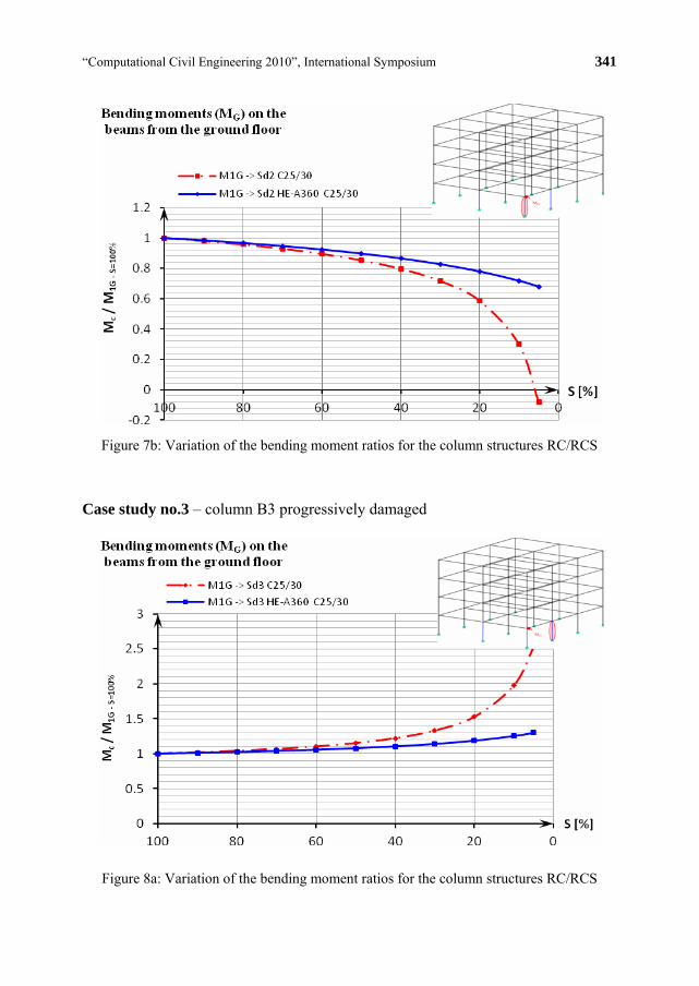
“Computational Civil Engineering 2010”, International Symposium 341
Figure 7b: Variation of the bending moment ratios for the column structures RC/RCS
Case study no.3 – column B3 progressively damaged
Figure 8a: Variation of the bending moment ratios for the column structures RC/RCS

342 O.M. Ioniţă, N. Ţăranu, M. Budescu
Figure 8b: Variation of the bending moment ratios for the column structures RC/RCS
Case study no.4 – columns A2&A3 progressively damaged
Figure 9a: Variation of the bending moment ratios for the column structures RC/RCS

“Computational Civil Engineering 2010”, International Symposium 343
Figure 9b: Variation of the bending moment ratios for the column structures RC/RCS
Case study no.5 – columns A3&B3 progressively damaged
Figure 10a: Variation of the bending moment ratios for the column structures RC/RCS

344 O.M. Ioniţă, N. Ţăranu, M. Budescu
Figure 10b: Variation of the bending moment ratios for the column structures RC/RCS
7. CONCLUSIONS
The prediction of possible progressive collapse under specific conditions may provide very important information that could be used to control or prevent this undesirable event. It is now obvious that abnormal loadings must be taken into account when designing structures exposed to unexpected loads.
Abnormal load events could arise from a number of sources: gas explosion, confined dust or vapor conflagration, machine malfunction, high explosive effects, vehicle impact, aircraft or missile impact etc. However, up to date, no adequate tools exist that can perform a progressive collapse analysis with acceptable reliability. Therefore, in the design phase, it is very important to predict the behavior of possible progressive collapse, as accurately as possible, for the various abnormal loads that should be considered.
One should be able to define a desired stable state of a partially damaged or partially collapsed structure for various abnormal loads and local damage combinations. Such collapsed cases and the damage evolution rate should be determined. Since the building after a partial collapse might still be exposed to a next critical phase, the residual capacity of a partially collapsed structure will determine its robustness, accordingly. A damaged or partially collapsed structure could be very dangerous without enough information about its expected behavior.

“Computational Civil Engineering 2010”, International Symposium 345
The rapid prediction of future behavior, or the next phase of collapse, can increase the safety and confidence of both the occupants and rescue personnel.
For some specific types of buildings to which the risk of producing local damages exists, it is necessary to assume some case scenarios regarding the progressive collapse taking into consideration the necessary local measures for the preventing of global collapse.
One efficient way of improving the safety of reinforced concrete structures may be the use of composite columns with fully encased steel sections at the ground level since this is more likely to be exposed to impact loading.
When the total flexural stiffness of the concrete section is degraded in case of reinforced concrete safety (RCS) columns the effect of the encased steel section is felt by increases of maximum 35% of the internal force members of the adjacent elements, avoiding, in this way, the progressive collapse.
REFERENCES
1. Gilmour, J.R., Virdi, K.S., Numerical modelling of the progressive collapse of framed structures as a result of impact or explosion, Proceedings of the 2nd Int. PhD Symposium in Civil Engineering, Budapest, Hungary, 1998.
2. Griffiths, H., Pugsley, A., Saunders, O., Report of the Inquiry into the Collapse of Flats at Ronan Point, Canning Town, Her Majesty's Stationery Office, London, UK, 1968.
3. Val, D.V., Val, E.G., Robustness of Frame Structures, IABSE, Structural Engineering International (SEI), vol. 16(2), 2006.
4. Mendis, P., Ngo, T., Vulnerability Assessment of Concrete Tall Buildings subjected to Extreme Loading Conditions, Proceedings of the CIB-CTBUH International Conference on Tall Buildings, 8-10 May, Malaysia, 2003.
5. Tang, M., Kmetz, M.J., Hapij, A., DiMaggio, P., Ettouney, M., Designing for Progressive Collapse, Structure Magazine, April 2006, pp.13-17, 2006.
6. Krauthammer, T., Hall, R.L., Woodson, S.C., Baylot, J.T., Hayes, J.R., Sohn, Y., Development of progressive collapse analysis procedure and condition assessment for structures, Proceedings of Multihazard Mitigation Council Workshop on Prevention of Progressive Collapse, Rosemont, Illinois, 2002.
7. Taylor, D. A., Progressive collapse, Canadian Journal of Civil Engineering, vol. 2(4), 1975. 8. Ellingwood, B., Leyendecker, E. V., Approaches for design against progressive collapse, Journal
of the Structural Division, ASCE, vol. 104, no. 3, 1978. 9. Ellingwood, B.R., Load and Resistance Factor Criteria for Progressive Collapse Design, National
Workshop on Prevention of Progressive Collapse, Rosemont, Illinois, Multihazard Mitigation Council of the National Institute of Building Sciences, Washington, D.C, 2002.
10. American Society of Civil Engineers, ASCE 7-05: Minimum Design Loads for Buildings and Other Structures, 2005.
11. U.S. General Services Administration, GSA Progressive Collapse Analysis and Design Guidelines for New Federal Office Buildings and Major Modernization Projects, 2003.
12. Unified Facilities Criteria, UFC 4-023-03: Design of Buildings to Resist Progressive Collapse, 2003.

“Computational Civil Engineering 2010”, International Symposium Iasi, Romania, May 28, 2010
Advanced 3D Modeling in ArchiCAD. Basic GDL scripting
Paul Mutică1, Silivan Moldovan1, Ioana Moldovan2
1Faculty of Architecture and Urban Planning, University of Technical Sciences, Cluj-Napoca,
2Faculty of Civil Engineering, University of Technical Sciences, Cluj-Napoca
Summary
The purpose of this paper would be to try and synthesize the various techniques employed for creating specially shaped, advanced 3D models in ArchiCAD, different from the ordinary methods available to general users of the program that can create basic shapes.
For this, it would be interesting to attempt an introduction in the platform interface, a possible, rudimentary, explanation of how the program works and how it is used to develop the BIM (Building Informational Model) of a construction.
Also it would be needed to underline some differences in concept and workflow between Graphisoft’s ArchiCAD and the other BIM oriented platforms used today in architectural computer aided design, like AutoDesk’s AutoCAD, Revit or Nemetschek Allplan.
Following that, it would be necessary to mention some of the late version’s (ArchiCAD 13.0) improvements over the previous ones, methods that ease a lot the work effort of the designer and help better correlate all views like, for example, the trace option or 3D dimensioning.
The next chapters will be concerned with the creation, grouping and possibilities of editing some basic 3D objects in order to construct more elaborate objects that are not already available in ArchiCAD’s libraries. For this purpose, some tools like the complex profile manager, the truss maker, roof maker and solid element operations would give an idea of how one can originally bypass some of the initially perceived limitations of the platform.
Finally, the main purpose, as stated, would be to give a minimal grasp on GDL objects, their creation, editing, export and import to and from other programs such as AutoCAD, 3D Studio Max or other rendering specialized platforms. Also, GDL scripts offer unlimited shapes and options for those who are not afraid to familiarize themselves with scripting language.
KEYWORDS: 3D, modeling, design, CAD, ArchiCAD, GDL scripting.

“Computational Civil Engineering 2010”, International Symposium 347
1. INTRODUCTION
During the second half of the 20th century, the drawing and copying technology of projects evolved, from duplicating machines that used carbon paper, Photostat, mimeograph machines, until the development of the photocopier by Xerox around the 1960’s.
But these were mere surface changes as they only allowed for easier multiplication and were even discredited for increasing the bureaucracy needed to promote a project.
The real changes came during the 1980’s and 1990’s when Computer Aided Design (CAD) was introduced to act as a drawing tool for the architect or engineer. Time was considerably shorter for elaborating the drawing using CAD and corrections were made much easier than directly on paper.
The latest era in development of design starts from the concept of 3D editing of a virtual building. The BIM (Building Informational Model) transforms CAD into a tool were specialists could actually design a new object and test it for errors on their computer and has the unique advantage of correlating any change into all the documentation pieces (plan, sections, elevations) of the project released for execution afterwards.
The 3D model of a building can also be used to fashion photo realistic images, animations to impress the viewers or even simulations and tests for several problems, including seismic and atmospheric.
It would seem that the virtual building has evolved far beyond the blueprints of the older ages and that this progress is undeniably easing up the process of design and execution but there are people who contest that the virtual buildings and rendering animations are all positive in the future development of the building.
In order to understand how the programs work in implementing the 3D model of a building and to use them for their maximum capacity, not just as a simple drawing device but a simulation of a real object, we have to attempt a minimal incursion in the language that programmers used to define their environment. If we take ArchiCAD, for example, one can easily use a lot of fully editable objects already present in the library but, after a while, will find them in short supply and will desire to create new ones to suit personal purposes.
This might seem a little too much for the average user who does not have any background in information technologies and computer science but, hopefully, this paper will prove it to be far less strenuous than previously anticipated.

348 P. Mutică, S. Moldovan, I. Moldovan
2. ARCHITECTURAL CAD APPLICATIONS IN USAGE
Starting from around 2002, CAD applications have slowly adopted a different approach towards design in general, namely a tendency to replace the old 2D line based drawing with a 3D model of the projected object.
Programs used in architecture design include AutoDesk’s Revit and AutoCAD Architectural Desktop, with almost two thirds of the market divided between them and Graphisoft’s ArchiCAD with roughly 30% of the users.
Other BIM applications include Bentley Architecture, Digital Project, Tekla Structures and Nemetschek Allplan all around 5% of the total number of users or less(1).
From the now legendary AutoCAD platform and its cumbersome first versions of the 1980’s, to today’s specialized branches for every technical aspect of the project, architecture, engineering, presentation, and so on, CAD applications have improved enormously.
At first, even navigating through the whole worksheet, panning and zooming in and out was a problem, the selection and generation of lines and fills was a back-breaking work.
Now you can literally sketch in 2D and 3D, you have easily accessible filters for grouping, selecting, assigning properties of elements from one another and, most importantly, correlation between all aspects of the drawing, both 2D and 3D. So if you change a window, for example, in elevation or plan, it will be changed in the 3D model instantly, eliminating many errors.
The various CAD platforms mentioned above that are in use with today’s architects and engineers are in a constant competition for attracting clients and seizing the market and have generally moved towards a much needed “user-friendliness” in their interface.
The great leap forward was indeed achieved when the 2D drawing, that was only a historical design convention adopted by humans but inaccessible to the computer (and many humans who lacked spatial vision, for that matter) as a language in itself, was dropped in favor of the 3D virtual world model, that was easily implemented for the computer to read and use.
It is true that even today, because of the bureaucracy regarding the projects, 2D pieces of the project are fundamental for approving by the authorities and execution but the visionaries envision a 3D or even 4D project for these phases also in the future(2). Even today, most platforms, including Revit, ArchiCAD and Nemetschek Allplan generate their 2D drawings from the 3D model directly, not from human error prone projections of the elevations or sections.

“Computational Civil Engineering 2010”, International Symposium 349
Today, specialists tend to use virtual reality elements similar to the real ones, such as walls, beams, columns and roofs, all with their specific characteristics that have several advantages:
first, they are incredibly easily accessible to the human user because they are so familiar in essence to our environment,
second, they are easier for the computer to generate because they have restricted parameters of deformation given by rules and aspects of real life (you can only place a door and a window inside a wall, for example or you can only generate a slab as a prism, with according properties)
third, by using real-like elements you save time for editing their properties (as they are stored in libraries with real-like parameters already set for them) and constructing the model looks more like a Lego game or a puzzle than a drawing
fourth, the use of these elements, as they appear also in all 2D documentation pieces of the project, helps eliminate human errors
But not every 3D model is BIM. Though it may be part of a BIM, the 3D model alone is only an approximation of reality. The BIM concept goes even further, by adding the “information” (the “I” in “BIM”) to the model, making it perform actions similar to reality and send feedback to the architect or engineer(3).
Chuck Eastman, Director of AEC Integration Laboratory, expands the concept of BIM to a process. “The process of BIM is revolutionary because it provides the opportunity to migrate from practices that are centered around human craftsmanship to a more augmented and modern machine craftsmanship - and all that this might imply” and “BIM supports on-line simulation of a design, on-line simulation of construction - called 4D CAD” (4).
3. ARCHICAD 13. LATEST FEATURES
The programme that will be discussed, Graphisoft’s ArchiCAD 13 is currently the latest version available on the market. It has, as the large number of prior versions attest, made a lot of progress in understanding user needs and making their job easier.
The leap from earlier versions is not considerable; it mainly introduces a more complex trace tool that will enable the user to set any drawing as the background of the blueprint for reference. The other major change is the introduction of the three-dimensional system that allows for dimensioning of the object in the 3D window.

350 P. Mutică, S. Moldovan, I. Moldovan
Major leaps from even earlier versions include the new curtain wall tool the tracker, visual aid for selecting objects that overlap and so on.
3.1 Program Overview
ArchiCAD differs from other BIM platforms because, by having specialized objects (i.e. walls, beams, slabs, roofs etc.), they are optimized for 3D rendering (easier calculated by the machine) and thus take a lot less computer memory to generate and to move through. As a downside, this optimization means that certain parameters of these elements are fixed (for example slabs are always horizontal).
This, in turn, makes ArchiCAD somewhat easier to learn and manipulate even on a lower performance computer but means that it loses a certain amount of flexibility in terms of the shapes that it provides the user to chose from and work with. Or, at least this is the first impression one gets from working with it.
There are, however, several ways to bypass the lack o freedom in editing everything at an object and creating every type of shape one can imagine. Firstly, it is only fair to say that most pre-definite objects have a lot of editable parameters that satisfy most of the casual users.
Basic shapes section of the library includes, as the name states, some objects that might be commonly used by architects but don’t fall under the general categorization of walls, slabs or roofs (i.e. spheres, cones, cylinders, tubes, etc).
Some objects, for example the mesh tool for generating terrain can be used to define complex shapes either if 3D coordinates of specific points are known, or through simple use of moving nodes in the 3D window either vertically or horizontally. This will be addressed in the next chapter
For further editing, one can use the boolean or solid element operations tool to intersect objects, define parts that need to be subtracted or added to the original which becomes a target element as opposed to the operators. After the subtraction, the operator elements might be placed in an invisible layer as deleting them will cancel the previous operation.
ArchiCAD gives the user the capacity to save and edit his own 2D and 3D objects without any knowledge of GDL scripting – the informational language by which GDL objects are encoded into the platform. For an introduction into basic GDL scripting and object editing, one might refer to the “ArchiCAD Creating GDL Objects Interactive Training Guide” provided by Graphisoft on their website.
The following chapter will give an overview of the information presented in the training guide and give certain examples so as to familiarize the reader with the basic notions of GDL scripting.

“Computational Civil Engineering 2010”, International Symposium 351
4. BASIC MODELLING. CREATING GDL OBJECTS
The first example is the easy three step transformation of a 2D vectorial image of a topographic representation into a 3D model of the terrain using the mesh tool and modifiers like the magic wand tool.
Supposedly the topographic representation in fig. 1 will have to be transformed into a 3D model of the actual terrain. First one should generate a rectangular mesh that covers the entire drawing and then use the 2D splines to define auxiliary points on the mesh surface. To do this, it is sufficient to just select the mesh, keep the mesh button in the toolbox highlighted and, while pressing the spacebar, simply click on the splines in consecutive order. This will open a dialogue box that will ask to generate additional nodes on the mesh surface, following the splines, and to fit them to the user ridges. Pressing ok will add the points.
To elevate these points in 3d, one would simply have to click on them, and, when the small editing box appears, to select the elevate mesh point button and introduce the nominal height in meters. Checking the “apply to all” box will make all points along the spline elevate accordingly. Repeating this operation for all the other splines but with different elevations will generate a complex and realistic model of the terrain. One can remove the redundant triangulation lines afterwards in order to create a smooth terrain surface (fig. 4) and even disable the show all ridges so these triangulation lines will not appear in the plan view. .
. Fig. 1. Floor-plan view Fig. 2. Mesh creation
Fig. 3. 3D model of terrain Fig. 4. Smooth 3D model with highlighted curves

352 P. Mutică, S. Moldovan, I. Moldovan
The important aspect with this tool is that, provided the right spatial coordinates (derived from triple projection on the three planes, vertical, horizontal and lateral), one can create any shape that has a flat bottom and a variable top. Its limitation is that only the top of the mesh can be modeled, the bottom itself being flat unless being cut with solid elements operations.
A second useful tool in creating special shapes would be the custom profile wall. It basically acts like a wall but, instead of the normal rectangular section, any section can be extruded alongside the wall axis. It is especially useful for classical decorative elements such as moldings and for atypically shaped windows when in intersection with normal walls. The limitation is that it can only create objects extruded alongside a horizontal axis.
Fig. 5. Complex profile wall used Fig. 6. Editing the crown cornice profile to generate a cornice from the profile manager menu.
The third useful tool would be the trussmaker, which is especially used for creating iron or wood trusses. It functions simply by using a 2D representation in the floorplan to create a vertical section of the truss.
However, all these shapes are basically constricted in one way or another and cannot create every type of freeform shape. In order for more complex objects, one might consider using these basic shapes and adding them together or intersecting/substracting them with solid element operations.
4.1 Creating objects
Once a certain shape has been created, depending on the tool used to create it, there might be necessary to save it as a GDL object for further reference in this or another project. This might be an automatic process such as for stairs or trusses but it might not be necessary for simpler objects or objects created form a group of simple objects. But, if at any moment, the user decides to save his object as a GDL

“Computational Civil Engineering 2010”, International Symposium 353
object, all he has to do is to select File\Libraries and objects\Save 3D model as… He can then choose from saving the object as a GDL object, a door or a window.
Apart from this, one can use the newly created GDL object as a custom part of a more complex predefined GDL object such as a door panel to use with existing door type objects. In this case, the object will be created in the floorplan view as if the door would open in the horizontal plane and then it will be transferred automatically in upright position when placing the door with the custom panel just created.
Fig. 7. Creating and importing door panels for existing door objects(5)
The reader can download the “ArchiCAD Creating GDL Objects Interactive Training Guide” from www.graphisoft.com for further reference into how one can save models and create GDL objects gradually, from basic forms created in ArchiCAD to more complex ones, generated directly from GDL scripting.
5. BASICS OF GDL SCRIPTING
Chapter 6 of this Guide is particularly helpful as it introduces the user gradually to basic GDL scripting notions such as the Object Hierarchy, the ZZYZX parameter, the Local and Global Coordinate Systems, etc.
To begin creating a new GDL object, one must select the File\libraries and objects\ new object command. From there, the user must choose the subtype of the object to be created, in this case (a round, one leg table designed by Ben af Schulten, presented in the example – Fig. 8) a general Model Element subtype.

354 P. Mutică, S. Moldovan, I. Moldovan
Fig. 8. modeling Pedestal table P90 – designer Ben af Schulten(6)
Fig. 9. GDL parameters for Pedestal table P90(7)
Apart from the basic parameters available for any general Model Element Subtype, this design table will require, as Fig. 9 shows, several particular parameters such as the table-leg radius, the materials for the tabletop, table-leg and bottom, the total height or ZZYZX parameter, the tabletop thickness and its radius. Creating and

“Computational Civil Engineering 2010”, International Symposium 355
editing these parameters is clearly explained in the 8 video presentations of Chapter 6 of this guide.
Next it is time to create the geometry of the table, by using a succession of cylinders and cones generated directly from the 3D script window of the GDL object. Instead of using the dimensions of this particular design table, the user is instructed to use the parameters created to define it (Radius_Leg, Thickness_Top, Material_Top, etc) because these could be easily altered by further users directly from the object parameter settings in ArchiCAD infobox.
For example, the generic command to create a cone in GDL scripting would be: “CONE h, r1, r2, alpha1, alpha2” whereas for a cylinder, the scripting would be “CYLIND h, r”. In this particular case, the bottom of the table leg is a cone with these dimensions: “CONE .06, .25, Radius_Leg, 90, 90” where .06 is the height, .25 is the first radius, the second (upper) radius – that of the table-leg (Radius_Leg), whereas alpha 1 and 2 both equal 900 for a vertical cone. Introducing “CONE .06, .25, Radius_Leg, 90, 90”as the first line of the script would generate the bottom of the leg. Introducing “ADDZ .06” as the second line would shift the local coordinate system up by 0,06 cm in order to generate the next object, the cylinder leg and so on. The table 3D script is complete after introducing the parameters for the tabletop.
The final scripting should look like this: “CONE .06, .25, Radius_Leg, 90, 90 ADDZ .06 CYLIND .05, Radius_Leg ADDZ .05 Height_Leg = ZZYZX-Thickness_Top-.04-.05-.06 CYLIND Height_Leg, Radius_Leg ADDZ Height_Leg+.04 MULZ -1 CONE .04, .15, Radius_Leg, 90, 90 DEL 1 CYLIND Thickness_Top, Radius_Top DEL TOP”
The MULZ command inverts the Z axis in the coordinate system while the DEL 1 cancels the last command on the coordinate system. DEL TOP returns the coordinate system in its original, global location.
Apart from the 3D script and parameters tabs, GDL objects have several other variants, including the 2D script, master script, the 2D symbol, picture preview etc.
Thus, GDL scripting can be very laborious but it can yield particularly long term results because objects created once can be used in all further projects. The number

356 P. Mutică, S. Moldovan, I. Moldovan
of parameters can be huge and a system of grouping them and commenting on what’s their purpose is most important.
One such complex GDL object, created with GDL scripting but able to evolve into very different shapes in use would be the “tooth” object, currently under construction by Raoul Cenan(8). From what can be seen from its promising presentation by the author, tooth is more of a family than a particular object. It can easily be morphed into various shapes, from cubes, cones, prisms and spheres to more complex blebs, blobs, shreds or skins (Fig. 10 – 13).
Fig. 10. Auto-intersecting surfaces (Blebs) Fig. 11. Blob volume
Fig. 12. Membrane surfaces (Skins) Fig. 13. Combined surfaces (flower)
Tooth is based on Steven Coon’s formulae for surface patches and several teeth can be grouped for more complex shapes. Another aspect of this object is that the number of facets is variable so as to better approximate curves. It is one of the few objects in ArchiCAD that can reproduce three-dimensional quadrics and therefore

“Computational Civil Engineering 2010”, International Symposium 357
it is much needed especially since the lack of freeform objects was one of the few setbacks of ArchiCAD compared to other programs.
But perhaps the best thing about the object, if it will live up to the expectations, is that it comprises in easy form all editable parameters directly from the object default settings dialogue, meaning that no GDL scripting knowledge is required in order to handle it, thus decreasing considerably the amount of time needed to use it.
6. CONCLUSION
The rapid development of computer graphics and CAD has both adepts and critics who fear it might be too restrictive on imagination, despite all its qualities.
However, if one regards CAD or BIM as a tool for constructing a virtual building and not as a mere library of preexistent objects that he has for assembling the construction, many of the problems concerning creativity, uniqueness and the quality of the design will simply be overcome. Regardless how the object was created, the quality of the project is still in the hands of the architect and, no matter how developed the CAD platform, it is, after all, only a tool.
As proven, ArchiCAD has the tools necessary for quality design and architecture but, just like any other tool of its kind, it does not guarantee the results by itself.
References
1. According to a survey of Bentley Systems launched in July 2007 and quoted by Raoul Cenan in From CAD to BIM, LogiA, No. 10 (October 2008), ISSN 1454-8771, p 80
2. Chuck Eastman, Paul Teicholz, Rafael Sacks, Kathleen Liston, BIM Handbook, a Guide to Building Information Modeling for Owners, Managers, Designers, Engineers and Contractors, John Willey & Sons Inc., Hoboken, New Jersey, ISBN 978-0-470-18528-5, p 16
3. U.S. General Services Administration, 3D-4D Building Information Modeling, http://www.gsa.gov/Portal/gsa/ep/contentView.do?contentType=GSA_OVERVIEW&contentId=20917
4. Chuck Eastman, What is BIM?, http://bim.arch.gatech.edu/content_view.asp?id=402 5. ArchiCAD Creating GDL Objects Interactive Training Guide, Chapter 4, www.graphisoft.com 6. Idem, Chapter 6.1, Overview 7. Ibidem 8. TOOTH, The Topological GDL Cube, ArchiCAD Spring Academy, 14-15 may 2010, Pula,
Raoul Cenan, Faculty of Architecture and Urban Planning, Technical University of Cluj-Napoca http://www.archicadspringacademy.com/ArchiCAD_Spring_Academy/agenda.html

“Computational Civil Engineering 2010”, International Symposium Iasi, Romania, May 28, 2010
Shielding Mortar Design for Protection of Rooms Exposed to X-Ray
David Procházka1, Jiří Brožovský2, Vít Černý3 1 Institute of building Materials and Components, Faculty of Civil Engineering , Brno University of
Technology, Brno, 662 00, Czech Republic 2 Institute of building Materials and Components, Faculty of Civil Engineering , Brno University of
Technology, Brno, 662 00, Czech Republic 3 Institute of building Materials and Components, Faculty of Civil Engineering , Brno University of
Technology, Brno, 662 00, Czech Republic
Summary
The paper presents shielding mortar design intended primarily to protect persons against the harmful X-ray. Such mixtures are standardly used when building workstations with X-Ray devices (Hospitals, laboratories, nuclear plants, etc.). Their main characteristic is the high volume weight. According to theoretical models and practical knowledge, this is precisely the main factor influencing effectiveness against the X-ray radiation. High density is achieved by using heavy filler. This is mostly rock, but also used steel filings and iron pigs. When designing such mixture, technologist must take into account different behaviour as: heavy components segregation or worse flow properties. Essentially, the principle is the same as by the standard mortar design. But always it is necessary to closely monitor tests implementation and evaluation. Just so we can avoid potential problems when building.
KEYWORDS: barite, shielding, ionizing radiation
1. INTRODUCTION
The submission refers on previous research on the field of radiation protection, which was carried out on the Institute of Building Materials and Components in Brno. In this framework it has been developed baritic mortars that varied by the used binder and filler granulometry (results were also presented at the CCE 2008 and CCE 2009). The best seems to be mortars, where the binder was cement and filler barite sand. Mortars with ash as partial binder replacement showed with mortars where the barite dust filler were used lower strength and worse shielding ability. Lower strength is caused due to ashes latent hydraulicity and due to higher need for water by the dust. Worse shielding ability relates then to a lower density of hardened mortar. These mortars yet demonstrated the applicability and have

“Computational Civil Engineering 2010”, International Symposium 359
been used in practice in the construction of radiation centers. The present submission reflects tests performed on the barite mortar with cement binder and barite dust. [1, 2, 3, 4]
2. APPLIED RAW MATERIALS
For the cement mortar design were used CEM I 42,5 N Ladce and barite dust from the separation unit. Materials were the same type and origin, as in previous work. Their main characteristics can be seen in Tables 1, 2.
Table 1. Barite dust sieve analysis Mesh size (mm) Intersieval (%) Undersizes (%)
0,2 0 100 0,12 0 100 0,09 0,09 99,91 0,063 2,17 97,74 0,045 5,25 92,49 0,032 8,32 84,17 0,020 14,47 69,70 0,010 22,55 47,15 0,005 18,24 28,91 0,001 23,21 5,70
< 0,001 5,7 0 Σ 100
Barite dust gradation curve
0
10
20
30
40
50
60
70
80
90
100
< 0,001 0,001 0,005 0,01 0,02 0,032 0,045 0,063 0,09 0,12 0,2
Sieves mesh sizes [mm]
To
tal u
nd
ersi
zes
in %
of
the
mas
s
Figure 1. Barite dust grading curve

360 D. Procházka, J. Brožovský, V. Černý
Table 2. Properties of cement provided by the manufacturer Parameter Value
Setting beginnig (min) 224 Compressive strength after 2 days (N·mm-2) 21,6 Compressive strength after 28 days (N·mm-2) 49,4 Specific surface (m2·kg-1) 329 Cr content (VI) (mg·kg-1) 0,61
3. MIXTURE DESIGN
At the design it was resulted from already known formulas. [3, 4] These were practicaly identical to the formula below. (Tab. 3).
Table 3. Designed mortar formula Parameter Value
cement 12 barite dust 0-0,063 mm 88 Composition [%] admixtures 0,15
Dry mass Volume weight of the dry mixture in shaked state [kg·m-3]
2 940
Water-cement ratio [-] 0,39 fresh mixture 3 100 Bulk density of concrete
[kg·m-3] after 28 days of maturing 3 060
The resulting mixture had worse workability than similar barite sand mortar. Higher water need resulted from the fines amount. To obtain higher mortar strength the water reducing admixture were used.
4. TECHNOLOGICAL PROPERTIES
Hardened mortar properties were evaluated at prisms 40 x 40 x 160 mm (Tab. 4).
Table 4. Hardened mortar properties (barite dust) Parameter Value
Water-cement ratio [-] 0,39 after 1 day 0.7 Bending tensile strength
[MPa] after 28 days 3,1 after 1 day 4,3 Compression strength
[MPa] after 28 days 15,9

“Computational Civil Engineering 2010”, International Symposium 361
For comparison, in Tab. 5 there is showed similar formula with barite sand. [3]
Table 5. Hardened barite sand mortar Parameter Value
Water-cement ratio [-] 0,29 after 1 day 1,6 Bending tensile strength
[MPa] after 28 days 3,3 after 1 day 6,6 Compression strength
[MPa] after 28 days 22,4
From the comparison the difference in the strength and need for water is significant. Low strength limits "dust mortar" in the using possibility. For bearing purposes it practically does not fit.
5. SHIELDING PROPERTIES
Like the previous tests, this mortar was tested for shielding capabilities too. They were tested on plates of different thicknesses. Barytic samples were radiated by macro-structural X-ray apparatus. Tested were various thicknesses and radiation intensities.
1
100
10000
1000000
Do
se r
ate
(pG
y/s)
60 80 100 135
Voltage (kV)
Lead 4 mm
Lead 3 mm
Slab 50 mm
Slab 40 mm
Slab 30 mm
Slab 20 mm
Slab 10 mm
Figure 2. Shielding properties for barite dust slabs
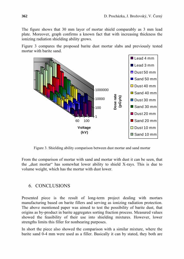
362 D. Procházka, J. Brožovský, V. Černý
The figure shows that 30 mm layer of mortar shield comparably as 3 mm lead plate. Moreover, graph confirms a known fact that with increasing thickness the ionizing radiation shielding ability grows.
Figure 3 compares the proposed barite dust mortar slabs and previously tested mortar with barite sand.
1
100
10000
1000000
Do
se r
ate
(pG
y/s)
60 100
Voltage (kV)
Lead 4 mm
Lead 3 mm
Dust 50 mm
Sand 50 mm
Dust 40 mm
Sand 40 mm
Dust 30 mm
Sand 30 mm
Dust 20 mm
Sand 20 mm
Dust 10 mm
Sand 10 mm
Figure 3. Shielding ability comparison between dust mortar and sand mortar
From the comparison of mortar with sand and mortar with dust it can be seen, that the „dust mortar“ has somewhat lower ability to shield X-rays. This is due to volume weight, which has the mortar with dust lower.
6. CONCLUSIONS
Presented piece is the result of long-term project dealing with mortars manufacturing based on barite fillers and serving as ionizing radiation protection. The above mentioned paper was aimed to test the possibility of barite dust, that origins as by-product in barite aggregates sorting fraction process. Measured values showed the feasibility of their use into shielding mixtures. However, lower strengths limits this filler for nonbearing purposes.
In short the piece also showed the comparison with a similar mixture, where the barite sand 0-4 mm were used as a filler. Basically it can by stated, they both are

“Computational Civil Engineering 2010”, International Symposium 363
comparable, though the “sand mortar” shows better shielding parameters, not to mention the better strength. Despite to somewhat inferior properties of “dust mixture” it is possible, considering the economic aspects, to utilize this mixture either for less demanding uses or adding barite sand for standard shielding constructions.
Acknowledgements
The work was supported by the MSM 0021630511 plan: Progressive Building Materials with Utilization of Secondary Raw Materials.
References
1. Pospíšilová, P., Fridrichová, M., Hoffmann, O. Využití sekundárních surovin pro přípravu stínicích barytových směsí. 4. konference speciální betony. Ostrava, Česká republika, 2006. ISBN 80-86604-27-6. (in czech)
2. Martinec, P., Brožovský, J. Vztahy pro predikci pevností směsných cementů. Maltoviny 2004. Brno, Česká republika, 2004. ISBN 80-214-2806-6. (In czech)
3. Procházka, D., Beneš, D. Gamma Radiation Shielding. Computational Civil Engineering 2008. Iaşi, România.
4. Procházka, D., Beneš, D. Barite Mortar with Fluid Fly Ash as Shielding Material. Computational Civil Engineering 2009. Iaşi, România.
5. ČSN EN 1015-3 Zkušební metody malt pro zdivo – Část 3: Stanovení konzistence čerstvé malty (s použitím střásacího stolku). (in czech)
6. Vavřín, F. Maltoviny. VUT v Brně, Praha 1980. (in czech)

“Computational Civil Engineering 2010”, International Symposium Iasi, Romania, May 28, 2010
High Strength Concrete Design Problematics
David Procházka1, Klára Křížová1, Tomáš Melichar1 1 Institute of Building Materials and Components, Faculty of Civil Engineering, Brno University of
Technology, Brno, 662 00, Czech Republic
Summary
Concrete structures design is an important part of the building industry. Concrete is extremely versatile material with very wide range of applications. Ever since antique times it is used for various purposes. Found very wide application and is used practically at every turn. This article is dedicated to high strength concrete, which is gradually becoming indispensable especially in economically important buildings. There will be shown benefits of its use and special features in its design. Compared to normal concrete, it is necessary carefully work and calculate a number of factors. Only a thorough and accurate design substantiated by responsibly performed tests, enables produce high strength concrete to the satisfaction of both the investor and contractor.
KEYWORDS: High Strength Concrete, Concrete Design,
1. INTRODUCTION
According to ČSN EN 206-1 high strength concrete is the concrete of class higher than C 50/60 (for ordinary and heavy concrete). For lightweight concrete the class must be higher than LC 50/55. High strength is achieved by low water dose, higher cement content and properly chosen formula. These concrete advantages are particularly high strength as well as higher durability and less ductile deformation behaviour under load. Due to these properties it can be designed static very ambitious constructions too. Additional advantage is that the component crossection can be reduced and the space within building can be better used.
Using HSC goes back to the 60th last century, when in U.S. and Canada began testing stronger concrete for high-rise buildings. This concrete differed from the ordinary concrete by careful aggregates selection and rigorous technological discipline observance. Strength neared to 60 MPa by the slump test of 100 mm.
With higher strength pursuit first plasticizers cames to the word’s, soon followed by superplasticizers, that despite the variable quality shown the possibility for water amount reduction in the fresh mixture and thus increase the strength. In addition the concrete fluidity increased, the abrasion resistance improved, the modulus of elasticity increased and the permeability decreased. Thanks to

“Computational Civil Engineering 2010”, International Symposium 365
superplasticizers the HSC has a stronger contact zone between cement matrix and aggregates grains. With time the water-cement ratio could be reduced to the border under 0,30 and slump test of 200 mm. Step by step the compressive strength neared to the limit of 100 MPa (equivalent to water pressure in 10 km depth). Today it can be designed concrete of more than 120 MPa strength, however their practical use is limited due to higher costs. [1, 3]
2. RAW MATERIALS
In the high strength concrete production it is good to pay attention to the raw materials selection and quality. It is fact, that with today’s superplasticizers using it is not problem to reach 100 MPa, however, the raw materials selection can not be neglected. Important is e.g. the binders-admixture compatibility, aggregates quality, binder properties, etc. Only a careful components selection and their knowledge allows to prepare quality concrete proposal with constant properties.
2.1. Cement
From a strength point of view it is important that Portland cement develops as much dense C-S-H as it can, because calcium silicates (which represent about 80 % of the total mass of Portland cement) are responsible for strength development in concrete. This can be achieved by decreasing the water-binder ratio, but it should be taken into account the impact on rheology too. It must also be set the balance between sulphate, calcium and aluminium ions, otherwise the problems with setting may occur.
Very important role plays C3A (its cubic form). As known, C3A, sulphate ions and water generates ettringite – fast concrete setting. Therefore the setting regulator is added to the cement. By mixtures with low water-cement ratio the setting regulation is especially important. Simply told, the less C3A in cement, the better for the rheology.1 The cement properties plays a major role for the rheology. With most of cements it can be reached 100 MPa, however some of them may then have significant problems with the rheology. If we want to achieve higher strength (above 125 MPa) the cement choice is very important.2 At high strength values it is usually big problem to maintain a good rheology and workability sufficiently long to ensure uniform characteristics throughout the casting. It appears that the
1 For laboratories the C3A determination is no problem. More difficult is the modifications determination. 2 Can be easily find out by Blaine. For higher strength values the finer grinding is better.

366 D. Procházka, K. Křížová, T. Melichar
rheology is influenced by the interstitial phase, while strength is given by the silicate phase.
Present cements responds to standards indeed and are suitable for usual concrete, nevertheless for HSC can represent a problem. Therefore, in practice, better choose the best of the available cements or the least bad.
2.2. Superplasticizers
Another important step is the superplasticizers choice, because not all superplasticizer types and brands react in the same way with a particular cement.
The determination of the optimum dosage of a superplasticizer of a high strength concrete is not easy. It greatly depends on what is the most critical issue for the particular high strength concrete to be produced with a particular cement or cementitious system. If the long-term strength issue is the most critical, without any problems on the rheological side, it is preferable to work with the highest amount of superplasticizer and lowest amount of water possible. However, the superplasticizer dosage should never be much higher than the saturation point in order to avoid segregation and excessive set retardation. If it is the rheological properties that are critical and not the strength, it is best to make the concrete with the highest water-binder ratio and the highest amount of water that can be used to achieve the strength requirements, and to adjust the superplasticizer dosage in order to get the desired rheology. In an intermediate situation, the most economical balance between the strength requirement (lowest possible water-binder ratio) and the rheological requirement (highest water-binder ratio) has to be found for the particular cement and particular superplasticizer used. If there are problems with controlling the rheology (fast setting), the use of a retarder can help to solve the slump loss. [1]
2.3. Supplementary cementitious materials
High strength concrete can be made using Portland cement alone as a cementitious material. However, a partial substitution of Portland cement by one or a combination of two or three supplementary cementitious materials can be advantageous from an economic or a rheological point of view.
2.3.1. Silica fume
From a chemical point of view, silica fume is mostly composed of SiO2. Silica fume produced during the manufacture of silicon metal generally contains more than 90% SiO2. The specific gravity of silica fume is about 2 200 kg·m-3. The specific surface area ranges from 15 000 to 25 000 m2·kg-1. Because of their

“Computational Civil Engineering 2010”, International Symposium 367
fineness, silica fume particles can fill the voids between the larger cement particles. The filler effect is also said to be responsible for the increase in fluidity of concretes with a very low water-binder ratio. Owing to its unique physical characteristics, the resulting solid matrix including silica fume is very dense. Due to the extremely small size of silica fume particles, the addition of silica fume sharply reduces both the internal and the superficial bleeding in the mixture. This reduced bleeding is very important from a microstructural point of view because it drastically transforms the microstructural characteristics of the transition zone between cement paste and aggregates, and cement paste and reinforcing steel.
The usually dosage lies between 3 – 10 % of cement amount. With another addition there is only a small strength increase, but the costs rises.
2.3.2. Slag
Slag has a chemical composition that does not too much vary and lies within a well-defined area of the SiO2-CaO-Al203 phase diagrams. For utilization in concrete the slag should be in vitreous state.
The slag use in concrete is relatively infrequently, in most cases it is being used with silica fume. The dosage ranges usually between 15 – 30 % of cement quantity.
2.3.3. Fly ash
Fly ashes are very often different chemical and phase composition, because of various burning process conditions and various fuel types. They can appear as plain spherical particles, with a grain size distribution similar to that of Portland cement, or they can contain some cenospheres, i.e. hollow spheres. Most fly ashes are pozzolanic materials, but some can be non-pozzolanic, while others are selfcementitious. The use of supplementary cementitious materials is beneficial in making high strength concrete because they can result in a cost saving. Their dosage in the final mix depends on the desired early strength of the high strength concrete. When making the concrete design it should be considered the lower slag and fly ash initial strength values.
2.4. Aggregates
The selection of aggregates must be done carefully because, as the targeted compressive strength increases, the aggregates can become the weakest link, where failure will be initiated under a high stress. Compared with usual concrete, a closer control of aggregate quality with respect to grading and maximum size is necessary, since a primary consideration is to keep the water requirement as low as possible. It should be obvious that only well-graded fine and coarse aggregates should be used.

368 D. Procházka, K. Křížová, T. Melichar
Crushed hard and dense rocks, such as limestone, dolomite and igneous rocks of the plutonic type (granite, syenite, diorite, gabbro and diabase), have been successfully used as coarse aggregate in high strength concrete applications. The shape of the coarse aggregate is also important from a rheological point of view. During crushing, roughly equidimensional particles (also called cubic particles) should be generated, rather than flat and elongated ones. The latter are weak; they can sometimes be broken with the fingers and tend to produce harsh mixes requiring additional water or superplasticizer to achieve the required workability. Impact crushers used to be favoured over cone crushers because they produce more cubic particles. From a shape and strength point of view, the best aggregates to make high strength concrete seem to be glacial gravels or, even better, fluvioglacial gravels because they are generally made of the strongest and hardest part of the rocks crushed by the glacier, and have been thoroughly cleaned by the running water from the melting glacier. [1]
3. HSC MIX DESIGN
The objective of any mixture proportioning method is to determine an appropriate and economical combination of concrete constituents that can be used for a first trial batch to produce a concrete that is close to that which can achieve a good balance between the various desired properties of the concrete at the lowest possible cost. It will always be difficult to develop a theoretical mix design method that can be used universally with any combination of Portland cement, supplementary cementitious materials, any aggregates and any admixture because in spite of the fact that all the components of a concrete must fulfil some standardized acceptance criteria, these criteria are too broad; moreover, to a certain extent the same properties of fresh and hardened concrete can be achieved in different ways from the same materials.
As long as usual concrete was essentially a mixture of Portland cement, water, aggregates and sometimes entrained air, these methods could be used with a very good predictive value to design a concrete mixture having a given slump and 28 day compressive strength. This is no longer the case, because concrete is becoming a more complex material than a simple mixture of cement, water and aggregates and it is more and more difficult to predict concrete properties theoretically in spite of the fact that the use of computers facilitates complex calculations.
In the present state of the art, the successful fabrication of high strength concrete depends on a combination of empirical rules derived from experience, laboratory work and a great dose of common sense and observation. The most important factor in the mix design of a high strength concrete, much more than in the case of usual concrete mixes, is the selection of materials. All concrete ingredients are

“Computational Civil Engineering 2010”, International Symposium 369
working at, or near, their critical limits. The key to success in designing a high strength concrete mix is to find materials in which the weakest link is as strong as required to meet the performance requirements, while the stronger parts are not so strong that they lead to an unnecessary expenditure. Present design methods are only approximated. Generally it is recommended to use them only as a guide. [1]
CONCLUSION
The HSC problematic is a very interesting part of the concrete engineering, respectively concrete technology. From a theoretical point of view, the article briefly pointed to some fundamental aspects that must the engineer technologist take into account to properly design HSC. Nevertheless, the ordinary concrete is still more used, its replacing by HSC (HPC respectively) is perhaps a matter of time. As suggested in the article, this concrete has many benefits. Especially it is higher durability and lower material consumption. Due to its strength the HSC substantially enables to reduce the concrete elements thickness, which calculated on the ordinary concrete cubage, speaks in favour of the HSC. Material savings advantages will be surely important in the near future, when we can expect e.g. aggregates resources fall (quality aggregates runs relative quickly low). Another important aspect is the cement replacement possibility by admixtures such as fly ash. Yet it is not involved in the initial strength of the concrete composite, according to some studies it is very advantageous in terms of durability by time strength increasing and by armature corrosion protection. Actual HSC usage in ČR and many other countries is not too spread. Mainly due to the small investor awareness about its advantages and some builders reluctancy to change their ways. Experience of developed concrete countries such as Japan, Norway, USA and Germany indicates, that HSC is very prospective type of concrete.
Acknowledgement
The work was supported by the project: FAST-J-10-18: Strength-deformation characteristics valuation of modern concrete types.
References
1. Aïtcin, P.-C. Vysokohodnotný beton. Praha: Informační centrum ČKAIT, 2005. 320 p. ISBN 80-86769-39-9. (in czech)
2. Reiterman, P., Kolář, K., Huňka, P., Klečka, T. Dlouhodobý vliv druhu cementu a dávky příměsi na vývoj modulu pružnosti. Technologie betonu 2010. Pardubice. Česká republika. (in czech)
3. ČSN EN 206-1. Beton – Part 1: Specifikace, vlastnosti, výroba a shoda. Praha: Český normalizační institut, 2001. 72 p. (in czech)

“Computational Civil Engineering 2010”, International Symposium Iasi, Romania, May 28, 2010
Specific Pavement Condition Indicators for rigid and flexible
pavements
Elena Puslau1, Costel Plescan2
1Department of Roads and Foundations, "Gh.Asachi" T.U. of Iasi, Iasi, 700050, Romania, 2Department of Structural Mechanics, "Gh.Asachi" T.U. of Iasi, Iasi, 700050, Romania
Summary
Maintenance and rehabilitation oh roads pavements are one of the major problems faced today by pavement engineers and administration in the road transportation system. It is a real challenge and has been intensely studied during the last few years. The reality of insufficient funds to adequately repair pavements under an agency responsibility, the gap between needs and allocated funds and other financial problems are found in the heading of almost all technical reports and publication related to the topic. It is a problem which affects both rich and poor nations as well as developed and countries. Today no nation, state, or city administration is immune from this problem. Huge investments are required to upgrade the road system and to maintain it above the minimum established or desired levels. In the US more than $1 trillion has been invested in the highway system and maintain them above the minimum established or desired levels. This paper presents some aspects concerning the evaluation of performance of flexible and rigid pavements by using specific pavement conditions indicators developed around the world, with some proposal for feature implementation in the actual road practice in this country.
KEYWORDS: pavement management system, performance indicators, pavement condition, failure point, optimum rehabilitation point
1. INTRODUCTION
Most highway agencies have dedicated considerable effort to find solutions for this problem based upon sound management principle. The Pavement Management System (PMS) concept is directed to obtain the most efficient use of the highway funds. A very important portion of this efficiency must focus upon the maintenance and rehabilitation of highway network. The pavement structure is probably the most important part in the whole serviceability concept, as it consumes a large portion of the total investment. The pavement is also the interface between the user and road total investment and being exposed to all deterioration factors must be maintained in order to provide the minimum required level of service during the

“Computational Civil Engineering 2010”, International Symposium 371
entire design life. In recent years a great effort has been placed in the study of maintenance and rehabilitation of highway pavements.
A considerable amount of research has been conducted to develop new materials and procedures, as well as new techniques to study the performance and effectiveness of different strategies, to improve economic analysis, optimization procedures and several other areas related to the maintenance and rehabilitation concept.
2. HIGHWAY MAINTENANCE AND PAVEMENT DETERIORATION
Even with proper adherence to materials specification and design and construction techniques, highway pavements deteriorate with the passage of time. While most engineering structures have indefinite life, road pavements have a finite life and even with optional maintenance will reach a failure point, pavement structures being designed to fail within a specified time period. The deterioration mode will vary greatly as a function of the interaction of several parameters such as: the strength of the pavement structure, including the subgrade, traffic volume and axle loads and environmental conditions. A fourth component, maintenance policy is also a major parameter affecting the deterioration rate.
In general, pavement failure can be classified into structural and functional failure. Structural failure is associated with the load carrying capacity of the pavement and normally related to fatigue of the pavement structure. Functional failure is generally defined as the failure of the pavement surface to provide a smooth, safe, and economic ride to the users.
The deterioration modes are normally divided into load and non-load related. Load associated causes are directly induced by traffic upon the pavement structures. Non-load associated causes can be subdivided into environmental condition, construction quality and special problems. Among the most common non-load associated causes are: temperature, moisture, soil and site conditions, material variables, soundness of engineering design and constructions quality.
According to literature [1], the major types of distresses in flexible pavements are: fatigue cracking, pavement deformation (rutting), low temperature shrinkage cracking and disintegration.
Highway pavements may have different time-deterioration relationships of the particular combination of the numerous factors involved in the deterioration mechanism.

372 E. Puslau,C. Plescan
Figure 2.1, shows different deterioration curves as a function of pavement quality and time or load repetitions. What could be defined as a „typical curve” is also shown in the Figure2.1 discussed next. In general pavement condition suffers a fast and small drop in early stage of the pavement life. Then, the deterioration rate levels off to a minimum value and slowly increases, producing in a short period of time a dramatic reduction in the pavement condition. Thus, point C is reached and the pavement is considered failed. After that point the deterioration rate is considered failed.
good
time
PA
VE
ME
NT
CO
ND
ITIO
N
poor
Typical deterioration curve
A
B
C
Figure 2.1. Typical pavement deterioration curves
Along the evolution of this curve, in relation with Figure 2., there are several features upon which experts would agree and can be generalized for the majority of highway pavements as follows.
The failure point
The definitions of the failure point are one important aspect that must be deducted from this curve. For structures that must be not fail catastrophically, such as highway pavements, it is difficult to precisely define a failure point. The first difficulty is how to define pavement condition. The most widely used pavement engineering parameter is the Present Serviceability Index or PSI, which is an indicator of the ride quality of the pavement and assigns a pavement condition rating between 0 and 5 (5 being a perfect pavement). At the AASHTO Road Test, where this concept has been developed, the failure point was defined by a PSI value of 1.5. Today the most agencies have different levels of pavement failure as a function of road type and traffic volumes. These failure points, or minimum acceptable riding quality levels normally vary between 2 and 3. Figure 2.2. illustrates this concept showing some typical values.

“Computational Civil Engineering 2010”, International Symposium 373
PSI
time
Primary roads
1
2
3
4
5
Arterials/Collectors
Low volume roads
MINIMUM ACCEPTABLE LEVEL
Figure 2.2. Pavement performance curve. Typical PSI levels for different road types
Optimum Rehabilitation Point
The definition of the optimum rehabilitation point is the key to the solutions of many pavements problems, but at the same time is very difficult parameter to define. The typical deterioration curve (Figure 2.1.) shows a rapid deterioration between points B and C. The pavement quality drops from an acceptable level (B) to a failed level (C) in a very short increment of time when compared to the total pavement life. It is normally accepted, in general terms, that the restoration of the pavement to a as-new condition, will cost 4 or 5 times more if conducted when pavement reaches point C, compared to the required cost at point B. Thus, the relative short period of life between these two points represents a tremendous increase in the rehabilitation cost. The optimum time for time for rehabilitation is assumed to be close to point B.
In the pavement deterioration mechanism, this rapid reduction in the riding quality is normally explained as a consequence of the of traffic and environmental agents on a weakened pavement structure. Fatigued pavement surfaces develop cracks that permit water infiltration, which in turn, reduced the bearing capacity of granular bases and sub grade materials. Consequently, under traffic, larger deflections will occur accelerating the failure process by producing more cracks and permitting more water to enter the structure.
The concept of performance, user cost and maintenance and rehabilitation cost, are intimately connected along the time-deterioration curve. In figure 2.1., three points (A,B and C) were located on the typical performance curve. These points can be defined as:

374 E. Puslau,C. Plescan
Point A- the pavement begins to show minor deterioration symptoms that require routine maintenance (pothole repair, crack sealing, minor patching). An effective routine maintenance policy after this point, could be very important in controlling the deteriorating rate. It has been proved to be very cost-effective in the long run.
Point B- the pavement rate of deterioration begins to increase rapidly. It needs some type of surface and/or structural upgrading. This probably the optimum rehabilitation point where relatively moderate investment may produce large benefits. The pavement structure and riding quality are not badly deteriorated, the pavement structure still retains most of its original strength and any rehabilitation action will greatly improve the pavement condition and strength.
Point C- the pavement condition has fallen into a precarious structural or functional damage. Major rehabilitation work, normally requiring extensive patching, partial or total reconstruction, is required at this point.
3. DEVELOPMENT OF PRINCIPAL PAVEMENT CONDITION INDICATORS
The first step in the development of Program Rehabilitation system was to select a set of pavement condition indicators that could be combined in order to give the pavement engineer idea about the type of problem to be faced. In the selection of parameters the following criteria can be used:
the parameters must be selected among those widely used in the evaluation of highway pavements, particularly those employed for periodic evaluation and monitoring of pavement performance and as input parameters for PMS at the network level.
the selected parameter are easy to be determined, without major difficulties or sophisticated procedures and can be correlated with some of the different techniques to determine pavement condition.
Based on this criteria, the following parameters have been selected and used as primary input values in the various decision system:
Present serviceability Index (PSI)
Pavement Condition Index (PCI)
Pavement damage (consumed life)
Friction resistance (safety).

“Computational Civil Engineering 2010”, International Symposium 375
Present Serviceability Index
Present Serviceability Index (PSI) is the most accepted indicator of pavement condition from the functional standpoint. The serviceability concept was developed from the AASHTO Road Test and is used today as a common qualified of pavement quality and more important as a failure indicator. It rates the pavement from 0 to 5, with being 5 a perfect pavement. The PSI rates the pavement adequacy and provides quantitative indicator of the pavement adequacy or sufficiency to provide a smooth, comfortable ride to the user. PSI establishes a relationship between a simple subjective rating by the users and a objective pavement measurement. The following equation was developed by AASHTO for flexible pavements.
5,03 1,9 log(1 ) 0,01 1,38PSI SV C P RD (3.1)
Where:
SV=slope variance
C=major cracking (ft/1000 sf)
P=patching (sf/1000 sf)
RD=rut depth (in)
It has been determined that PSI is mainly a function of slope variance, or the variation in pavement profile or roughness. Thus, a good correlation can be obtained by using the following simplified equation, on similar ones.
4,89 1,92 log(1 )PSI SV (3.2)
PSI is a worldwide accepted concept, relatively easy to determine by different devices and procedures and used by many pavement agencies.
Pavement Condition Index (PCI)
In the selection of maintenance and rehabilitation alternatives the physical evaluation of pavement distress is of vital importance.
The Pavement Condition Index (PCI) is based on data gathered from visual pavement surveys. PCI was developed by the US Army Construction Engineering Research Laboratory and the methodology for its evaluation has been standardized [3]. The method is simple to use and is based on the observations of severity and frequency of 19 different distress types affecting the pavement condition as shown in Table 3.1. The rating scale is shown in Figure 3.1. the PCI value is obtained by subtracting from 100, deduct values (DV) determined from a chart for each distress mode.

376 E. Puslau,C. Plescan
Table 3.1. Distresses in flexible pavements PCI method Number Distress descriptions 1 Alligator cracking
2 Bleeding 3 Block cracking 4 Bumps and sags 5 Corrugation 6 Depressions 7 Edge cracking 8 Joint reflections cracking 9 Lane/shoulder drop off 10 Longitudinal and transversal cracking 11 Patching and utility cut patching 12 Polished aggregate 13 Potholes 14 Railroad crossing 15 Rutting 16 Shoving 17 Slippage cracking 18 Swell 19 Weathering and raveling
Table 3.2. Distresses in rigid pavements PCI method Number Distress descriptions 1. Blow up/Buckling
2. Corner Break 3. Divided Slab 4. Durability Crack 5. Faulting 6. Joint Seal 7. Lane/Shoulder 8. Linear Cracking 9. Patching (Large) 10. Patching (Small) 11. Polished Aggregate 12. Poouts 13. Pumping
14. Punch-out 15. Railroad Crossing 16. Scaling 17. Shrinkage 18. Spalling Corner 19. Spalling Joint

“Computational Civil Engineering 2010”, International Symposium 377
Figure 3.1 Flowchart for Determination of PCI.
STEPS IN DETERMINING PCI OF A PAVEMENT SECTION according ASTM Designation: ” Standard practice for roads and parching lots pavement condition index survey’s “ D6433-99
Step1 Divide pavement section into sample units sample units determine distress types and severity levels and measure density.
Step 2 Inspect sample units sample units determine distress types and severity levels and measure density.
Lateral and transverse cracking
Modern alligator
Step 3 Determine deduct values [2]

378 E. Puslau,C. Plescan

“Computational Civil Engineering 2010”, International Symposium 379
Step 4 Compute total deduct value
Step 5 Adjust total deduct value [2]
Step 6 Compute pavement condition index (PCI) 100 – CDV for each sample unit inspected
Step 7 Compute PCI of entire section
Step 8 Determine pavement condition rating of section according [3] PCI100
85
70
55
40
25
10
0
Preventive maintenance
Major rehabilitation
Reconstruction
Pavement Damage
Pavement damage is an indicator of the percentage of life consumed at any given moment during the service life of a pavement. It is a very important parameter in the evaluation of the general performance of a pavement structure, the highways pavements being designed, to carry a certain number of pavements are load repetitions during their design lives.
Friction Resistance
Skid resistance (SR) is an indicator of safety associated with pavement surface characteristics. Most pavements are required to have a minimum SR as a function

380 E. Puslau,C. Plescan
of geometric design, posted maximum speed, environmental conditions and traffic characteristics.
3. EXAMPLE OF APPLICATION OF PAVEMENT CONDITION INDICATORS
In Table 4.1 are presented the values recorded by the investigating team from action for field inspection to identify and record types of distresses observed on the road sectors:
Table 4.1 Types of distresses observed on the road sectors Cod Type of distress Type of
distress observed
Severity level
Density level
Obs
#1 Alligator cracking
#2 Bleeding X M F
#3 Transverse and block cracking
#4 Bumps and sags X M F
#5 Corrugations #6 Depressions
#7 Edge cracking #8 Joint reflection cracking
#9 Shoulder drop off
#10 Longitudinal and transverse cracking, longitudinal joint cracking, wheel track cracking
X M F
#11 Patching-utility cuts #12 Polished aggregates
#13 Potholes X M O
#14 Railroad crossing
#15 Rutting
#16 Shoving
#17 Slippage cracking
#18 Swell
#19 Weathering and raveling X M F
Note : M – Medium F – Frequently O – Occasional

“Computational Civil Engineering 2010”, International Symposium 381
Table 4.2 Work sheet for PCI
Severity level Measure density Cod Type of distress
Distress weight
Reduce Mediu High Ocazional Frequently Extended
Deduct value
#1 Aligator cracking 5 0,4 0,7 1 0,5 0,7 1
#2 Bleeding 3 0,8 0,8 1 0,6 0,9 1 2,16
#3 Transverse and block cracking 10 0,4 0,7 1 0,5 0,7 1
#4 Bumps and sags 5 0,3 0,7 1 0,6 0,8 1 2,8
#5 Corrugations 5 0,4 0,8 1 0,5 0,8 1
#6 Depressions 10 0,5 0,7 1 0,5 0,8 1
#7 Edge cracking 3 0,4 0,7 1 0,5 0,7 1 #8 Joint reflection
cracking 3 1 1 1 0,5 0,8 1
#9 Shoulder drop off 2 0,4 0,7 1 0,5 0,7 1 #10 Longitudinal and
transverse cracking, longitudinal joint cracking, wheel track cracking
20 0,4 0,7 1 0,5 0,7 1 9,80
#11 Patching-utility cuts
5 0,3 0,6 1 0,6 0,8 1
#12 Polished aggregates
2 0,8 0,8 1 0,6 0,9 1
#13 Potholes 7 0,4 0,7 1 0,5 0,8 1 2,45
#14 Railroad crossing 2 1 1 1 0,5 0,8 1
#15 Rutting 5 0,3 0,7 1 0,6 0,8 1 #16 Shoving 2,5 0,3 0,6 1 0,5 0,8 1 #17 Slippage cracking 2,5 0,3 0,6 1 0,5 0,8 1
#18 Swell 3 0,4 0,7 1 0,5 0,8 1
#19 Weathering and raveling
5 0,3 0,6 1 0,5 0,8 1 2,4
PAVEMENT CONDITION GOOD (PCR) IGST 80,39
19,61
REFERENCES
1. Witczak W.M, Jugo A., ”Development of rehabilitation methodology Approach for flexible highway pavements”, 1993 2. USACE- CERL, Development of a Pavement Condition Ration Procedure for Roads, Streets and Parking Lots, vol1, vol2, M – 268, 1979 3. ASTM Designation: ” Standard practice for roads and parching lots pavement condition index survey’s “ D6433-99

“Computational Civil Engineering 2010”, International Symposium Iasi, Romania, May 28, 2010
Time behavior changing of a pavement structure depending on asphalt layer characteristics
Carmen Răcănel, Adrian Burlacu Department of Roads and Railways, T. U. C. E., Bucharest, Romania
Summary
The Romanian Norm used to design a pavement structure with asphalt layers stipulate the calculus of fatigue damage ratio at the bottom of asphalt layers and limit the vertical strain value at subgrade level. This is possible by establishing the stress and strain state using specialized software. In this norm, the recommended values for asphalt mixture stiffness are the minimum one given for an equivalent temperature of 15oC. However, what happen when the temperature changes? Moreover, what is the influence of the vehicle speed?
The stiffness decrease when temperature increase and when frequency decrease. In case of fatigue line, the level of strain is in relation with number of cycles of loading, i.e. traffic volume.
This paper has the goal to emphasize the time behavior changing of a pavement structure concerning to fatigue damage ratio at the bottom of asphalt layers and vertical strain at the subgrade level in a pavement structure under the action of Romanian axle loads. The calculus is based on stiffness experimental values obtained on asphalt mixture in Roads Laboratory of Technical University of Civil Engineering of Bucharest depending on temperature, frequency and number of load cycles. The results obtained from calculus are presented like influence graphs.
KEYWORDS: fatigue life, stiffness, asphalt mixture, pavement design.

“Computational Civil Engineering 2010”, International Symposium 383
1. INTRODUCTION
The vehicle traveling on the road exerts a dynamic loading on the pavement. The dynamic loading is characterized by its speed, duration of loading, headways and traffic volume. The response of the pavement structure under the dynamic loading is totally different from that under static loading. Traditionally, highway engineering emphasizes more on road pavement design, materials used and the durability of the roads but traffic engineering focus more on the operation side, for instance, speed, capacity, acceleration/deceleration and headways. More research is needed to investigate the interaction between vehicles and road pavement in a dynamic environment.
The mechanical design of asphalt pavement structures can be performed by constructing a multi-layer system. The mechanical behaviour of each individual layer is determined by various data being characteristic to the material of the layer, so to say, the thickness of the individual layers, as well as their stiffness moduli, Poisson-numbers and fatigue curves.
The French pavement design method consists in a pavement mechanistic analysis based on the Burmister multilayer elastic model (1943) (LCPC software ALIZE, 1982). In that model, the Huet-Sayegh behavior is taken into account with its equivalent elastic modulus at the 15°C French average temperature and a 10 Hz frequency. That frequency value is assumed to be equivalent to the standard 72 km/h French vehicle speed. Such semi-analytical calculations provide relatively good stress and strain fields for heavy traffic pavements but it is less satisfactory for flexible pavements with low traffic, for high temperature gradients and for the analysis of damages under slow heavy loads.
As it know, the Romanian Norm used to design a pavement structure with asphalt layers stipulate the calculus of fatigue damage ratio at the bottom of asphalt layers and limit the vertical strain value at subgrade level. This is possible by establishing the stress and strain state using specialized software, based on Burmister multilayer elastic model. In this norm, the recommended values for asphalt mixture stiffness are the minimum one given for a temperature of 15oC. These values are given in table based on the climatic type of the area where the road is designed (table 1) and they are coming from laboratory tests of indirect tensile on cylindrical samples (IT-CY: SR EN 12697-26, annex C), according to SR 174-2009 (table 2).
This paper has the goal to emphasize the time behavior changing of a pavement structure concerning to fatigue damage ratio at the bottom of asphalt layers and vertical strain at the subgrade level in a pavement structure under the action of Romanian axle loads. The calculus is based on stiffness experimental values obtained on asphalt mixture in Roads Laboratory of Technical University of Civil Engineering of Bucharest depending on temperature, frequency and number of load cycles.

384 C. Răcănel, A. Burlacu
Table 1. Stiffness modulus values for asphalt mixture ( values for pavement desgin)
Course type Climatic type I & II Climatic type III Asphalt mixture type
Stiffness modulus (E), Mpa wearing course 3600 4200 binder course 3000 3600
Asphalt mixtures with D80/100 bitumen type base course 5000 5600
wearing course 4000 4500 Asphalt mixtures with modified bitumen binder course 3500 4000
3300 4000
Asphalt mixture stabilized with fibers:- MASF 16 type, - MASF 8 type.
wearing course wearing course 3000 3600
Table 2. Limit values for asphalt mixtures stiffness modulus Asphalt mixture Stiffness modulus at 15oC,
MPa, min. Prepared with no paraffins bitumen for roads/ additives bitumen, for wearing course
4500
Prepared with no paraffins bitumen for roads/ additives bitumen, for binder course
4000
Prepared with modified bitumen, for wearing course 4500 Prepared with modified bitumen, for binder course 4000 Stabilized with fibers and with no paraffin bitumen for roads or modified bitumen, for wearing course MASF8 MASF12.5, MASF16
4000 4500
2. STIFFNESS MODULUS OF ASPHALT MIXTURES
The stiffness modulus of asphalt mixture is a fundamental property that gives information about how much the materials deforms under a given load and is closely related with the fatigue cracking and permanent deformation because of time temperature dependence.
Stiffness modulus S is a term introduced by Van der Poel to distinguish S from the modulus E of elastic responses:
Tt
TtS,
,)(
(1)
where t is the loading time;
T is the test temperature.

“Computational Civil Engineering 2010”, International Symposium 385
Complex modulus is the relationship between stress and strain when the sample is subjected to a sinusoidal waveform load depending on time (figure 1).
response = force
time
time
applied load = displacement
phase angle (delta)
Figure 1. Sinusoidal applied load and response
In case of a linear viscoelastic material, the complex modulus is characterized by norm (absolute value) and phase angle. The norm of complex modulus |E*| (dynamic modulus) is an indicator of material stiffness and is characterized by the two components, the elastic one, E1 and the viscous one, E2:
21 2*E E E 2 (2)
0
0*
E (3)
where: 0 is the stress amplitude;
0 is the strain amplitude.
The elastic or dynamic modulus of material (ignoring the viscous effects) may be determined by the ratio of the peak stress to strain amplitudes from the complex modulus test.
In linear elastic multi-layer calculations for instance the E* modulus is generally used as input value for Young's modulus.
So, the stiffness modulus is the absolute value of the complex modulus |E*|.
In European Norm SR EN 13108-20 three tests are stipulated for stiffness modulus determination:
- test applying Indirect Tension to cylindrical specimens IT-CY, according to SR EN 12697-26 Annex C. In this test the applied load (force) is constant in time. The loading time is (124 4) ms and the measured stiffness modulus is the mean of five pulses of applied load.

386 C. Răcănel, A. Burlacu
- Four Point Bending test on prismatic specimens 4PB-PR, according to SR EN 12697-26 Annex B. In this test the specimen is subjected to four-point periodic bending with free rotation and (horizontal) translation at all load and reaction points. The strain amplitude, constant in time, is maximum (50 3) microdef and the initial stiffness modulus shall be determined as the modulus for a load cycle between the 45th and the 100th load repetition.
- Two Point Bending test on trapezoidal specimens 2PB-TR, according to SR EN 12697-26 Annex A. In this test the strain amplitude is constant and less or equal to (50 3) microdef. The stiffness modulus is determined for 30s to 2 min.
The samples are deformed in their linear range, under repeated loads or controlled strain rate loads.
The test conditions for the three test exemplified above are stipulated in SR EN 13108-20 standard (table 3).
Table 3. Type testing according to SR EN 13108-20
Type of test Temperature [oC] Frequency or loading time
IT-CY 20 124s
4PB-PR 20 8 Hz
2PB-TR 15 10 Hz
3. PAVEMENT DESIGN DEPENDING ON ASPHALT MIX STIFFNESS
Starting from idea that flexible pavement design based on elastic multistrat theory it must be took on consideration the values obtained in laboratory for stiffness modulus of asphalt mixtures depending on testing conditions (temperature, loading, frequency), authors propose a road structure to do case studies, according with romanian norm for pavement design (table 4).
Based on test type used and testing conditions it was obtained in Roads Laboratory of T.U.C.E.B different values for asphalt mixture stiffness. (figure 2, 3, 4, 5 and 6).
Values of stiffness modulus Em are presented on table 5.
Correspondence between frequency of test in laboratory and vehicle speed it is presented in figure 7.

“Computational Civil Engineering 2010”, International Symposium 387
Table 4. Road structure proposed for calculation Road layer Layer
thickness , cm Stiffness modulus
MPa Poisson number
Asphalt mixture in wearing course
4
Asphalt mixture in binder course
5
Asphalt mixture in base course
6
Em 0.35
Foundation of crushed rock
20 500 0.27
Ballast foundation 30 260 0.27
Soil type P1 100 0.27
IT-CY
0
5000
10000
15000
20000
25000
0 5 10 15 20 25 30 35 40 45
Temperature, oC
Stif
fnes
s M
odul
us,
MP
a
MAMR16 BA16 MASF16a MASF16m-1 MASF16m-2 mean
2PB-TR
0
2000
4000
6000
8000
10000
12000
14000
16000
0 5 10 15 20 25 30 35 40 45
Temperature, oC
Stif
fnes
s M
odul
us
at 1
0Hz
and
50m
, M
Pa
MAMR16-10Hz BA16-10Hz MASF16a-10Hz MASF16m-2-10Hz mean
Figure 2. Stiffness modulus versus Figure 3. Stiffness modulus versus temperature for IT-CY test temperature for 2PB-TR test
4PB-PR
0
5000
10000
15000
20000
25000
0 5 10 15 20 25 30 35 40 45
Temperature, oC
Stif
fnes
s M
odul
us
at 8
Hz
and
50m
, M
Pa
MAMR16-8Hz BA16-8Hz MASF16a-8Hz MASF16m-1-8Hz MASF16m-2-8Hz mean
4PB-PR
0
5000
10000
15000
20000
25000
0 5 10 15 20 25 30 35 40 45
Temperature, oC
Stif
fnes
s M
odul
us
at 1
0Hz
and
50m
, M
Pa
MAMR16-10Hz BA16-10Hz MASF16a-10Hz MASF16m-1-10Hz MASF16m-2-10Hz mean Figure 4. Stiffness modulus versus Figure 5. Stiffness modulus versus
temperature for 4PB-PR test at 8 Hz temperature for 4PB-PR test at 10 Hz

388 C. Răcănel, A. Burlacu
0
5000
10000
15000
20000
25000
0 5 10 15 20 25 30 35 40 45
Temperature, oC
Mea
n V
alue
s of
Asp
halt
Mix
ture
Stif
fnes
sM
odul
us,
MP
a
IT-CY 4PB-PR-8Hz 4PB-PR-10Hz 2PB-TR-10Hz
Figure 6. Mean values of asphalt mix stiffness versus temperature for different type of tests
0
20
40
60
80
100
120
0 2 4 6 8 10 12 14 16 18
Test Frequency, Hz
Veh
icle
Spe
ed,
km/h
Figure 7. Vehicle speed versus test frequency
Using the program ALIZE5 (based on Burmister theory) it was establish stress and strain state in road structure under action of standard 115kN axle. So, it could be determined the fatigue damage ratio based on horizontal tension strain (r) at the bottom of asphalt layers, and vertical strain (z) at subgrade level. For calculation it was considered two values of traffic volume Nc for a perspective period of 15 years: 0.9 m.o.s. and 2 m.o.s.( m.o.s. means million of standard 115kN axle).
Correspondence between air temperature and asphalt layer temperature was considered according with Shell, 1978, figure 8.

“Computational Civil Engineering 2010”, International Symposium 389
Tabelul 5. Stiffness modulus calculation values for asphalt layers (Em) y = Ax2-Bx+C
Type of test Temperature,
(x) oC
A B C Stiffness Modulus,
(y) Em, MPa
IT-CY 0 5
10 15 20 25 30 35 40
12.574 926.21 17705
17705 13388 9700 6641 4210 2409 1235 691 77 5
4PB-PR-8Hz
0 5
10 15 20 25 30 35 40
7.1449 741.82 19923
19923 16393 13219 10403 7945 5843 4099 2712 1682
4PB-PR-10Hz
0 5
10 15 20 25 30 35 40
6.0825 712.43 20401
20401 16991 13885 11083 8585 6392 4502 2917 1636
2PB-TR-10Hz
0 5
10 15 20 25 30 35 40
4.0794 448.26 12921
12921 10782 8846 7115 5588 4264 3145 2229 1518

390 C. Răcănel, A. Burlacu
Figure 8. Characteristic relationship between Tm eff (monthly temperature effective in
asphalt layer) and MMAT (medium monthly air temperature) or Ty eff (annual temperature effective in asphalt layer) and MAATeff (medium annual air temperature effective) for
different asphalt sub-layers (Shell, 1978)
In graphics from figures 9, 10 and 11 are presented obtained results: increasing of fatigue damage ratio and of vertical strain at subgrade level with increasing of air temperature for both traffic volumes considerate.
Table 6 present the parameters of equations provided by graphics from figures 9 - 11.

“Computational Civil Engineering 2010”, International Symposium 391
0
1
2
3
4
5
6
0.0 5.0 10.0 15.0 20.0 25.0 30.0
Air temperature, oC
Fat
igue
dam
age
ratio
, R
DO
IT-CY, Nc = 2 m.o.s. 4PB-PR-8Hz, Nc = 2 m.o.s.
4PB-PR-10Hz, Nc = 2 m.o.s. 2PB-TR-10Hz, Nc = 2 m.o.s.
Figure 9. Fatigue damage ratio versus air temperature for different type of tests, 2 m.o.s. traffic volume
0
0.05
0.1
0.15
0.2
0.25
0.3
0.35
0.4
0.45
0.5
0.0 5.0 10.0 15.0 20.0 25.0 30.0
Air temperature, oC
Fat
igue
dam
age
ratio
, R
DO
IT-CY, Nc = 0.9 m.o.s. 4PB-PR-8Hz, Nc = 0.9 m.o.s.
4PB-PR-10Hz, Nc = 0.9 m.o.s. 2PB-TR-10Hz, Nc = 0.9 m.o.s.
Figure 10. Fatigue damage ratio versus air temperature for different type of tests, 0.9 m.o.s. traffic volume

392 C. Răcănel, A. Burlacu
150200250300350400450500550600650
0.0 5.0 10.0 15.0 20.0 25.0 30.0
Air temperature, oC
Sub
grad
e le
vel v
ertic
al s
trai
n,
z, d
ef
IT-CY 4PB-PR-8Hz
4PB-PR-10Hz 2PB-TR-10Hz
admissible strain, Nc = 2 m.o.s. admissible strain, Nc = 0.9 m.o.s.
Figure 11. Subgrade level strain versus air temperature for different type of tests
Table 6. Equations parameters for fatigue damage ratio (y) - air temperature (x), Nc = 2 m.o.s. dependence y = AeBx Type of test
A B R2
IT-CY 0.1262 0.1567 0.9391 4PB-PR-8Hz 0.0635 0.157 0.9967 4PB-PR-10Hz 0.0565 0.1578 0.993 2PB-TR-10Hz 0.1972 0.1203 0.9985
Table 7. Equations parameters for fatigue damage ratio (y) - air temperature (x), Nc = 0.9 m.o.s. dependence y = AeBx Type of test
A B R2
IT-CY 0.0099 0.1567 0.939 4PB-PR-8Hz 0.005 0.157 0.9967 4PB-PR-10Hz 0.0044 0.1578 0.993 2PB-TR-10Hz 0.0155 0.1203 0.9985
Tabelul 8. Equations parameters for subgrade level vertical strain (y) - air temperature (x) dependence
y = AeBx Type of test
A B R2
IT-CY 186.66 0.0251 0.9866 4PB-PR-8Hz 178.6 0.0195 0.9913 4PB-PR-10Hz 176.12 0.0196 0.9832 2PB-TR-10Hz 203.59 0.0156 0.992

“Computational Civil Engineering 2010”, International Symposium 393
3. CONCLUSIONS
Conclusion drawn from this article are:
- whereas differences exist between national norm SR 174 and the norm for flexible pavement design PD177 regarding the minimum required stiffness modulus of wearing and binder courses, is necessary to revise the norm PD177 (table 1 and 2);
- results from laboratory studies that, depending on asphalt mixture composition, one can obtain different values for stiffness modulus using the same equipement; more, using various equipements, according european norm SR EN 13108-20, 4PB-PR gives maximum values for stiffness modulus, regardless temperature, asphalt mixture and frequency; for temperatures below 13oC IT-CY test conduct to higher values compared with 4PB-PR test; in exchange, for temperatures over 13oC the situation is reversed (figure 6); to establish what test is more appropiate to provide the correct values for stiffness modulus, values which can be used in pavement desigining, it requires an experimental study on cores from field parallel with a study on samples made in laboratory.
- whatever type of test used, the stiffness modulus varies with temperature as: there is a decrease on average by more then 90% of the stiffness modulus when the temperature increases by 100% (from 0°C to 40°C), regardless of type of test, test frequency and asphalt mix type tested (figures 2 – 5); here it should be mentioned that a temperature of 40oC in 15 cm thick asfalt mixture means an air temperature of 30oC; in wearing course (4 cm thickness) for the same air temperature of 30oC it can be obtained a temperature of 50oC – temperature when the material has no longer an elastic behaviour (figure 8);
- due to climate changes in recent years (especially pronounced warming trend during the summer, overlaped with cold winters in our country) in the pavement design calculations should be taken into account temperature suscpetibility of asphalt mixtures by taking into account different stiffness modulus values, depending on temperature found in road;
- in pavement design calculation it must take into account the technical class of road, by considering the appropiate frequency of testing to obtain stiffness modulus, this being close related with vehicle speed: a frequency of 1o Hz correspond to a speed of 72 km/h (figure 7); it is known that stiffness modulus increase withe the increasing of frequency, at a given temperature;
- fatigue damage ratio decrease with the increasing of air temperature (figures 9, 10); for road structure chosen, considering a traffic volume of 2 m.o.s., if it is veriffied for fatigue at temperatures below 13oC-18oC, mean of 15oC (baesd of type of test used for stiffness modulus determination) it step up far over the eadmissible

394 C. Răcănel, A. Burlacu
value (it is recording an increase with 70% of RDO value) when temperature increase with 10oC (between 15oC and 25oC);
- the same as fatigue damage ratio, the strain at subgrade level increase with the increasing of air temperature (figure 11), recording the passing of admissible value (for a traffic volume of 2 m.o.s.) around temeprature of 15oC;
- laws of variation for RDO and strain z with air temperature are proposed, with the shape: y = AeBx;
- in conclusion, for flexible pavement design, it is necessary to establish minimum requirements concerning correlation of stiffness modulus with design speed, road temperature and technical class of the road.
References
1. C. Răcănel, A. Burlacu, C. Surlea, Establishing of wearing course asphalt mixture stiffness, First international Conference on Road and Rail Infrastructure, Opatija, Croatia, 17-18 May 2010
2. E.J.Yoder, M.W.Witczak, Principles of pavement design, 1975 3. Shell Pavement Design Manual - Asphalt Pavements and Overlays for Road Traffic, Ed. Shell
International Petroleum Company Limited, London, 1978 4. PD177-2001, Norm for flexible and semirigid pavement design(Analytical Method), B.T.R. no.1,
2001 (in Romanian) 5. SR 174-2009 Road works. Hot bituminous rolled pavements. Requirements for quality (in
Romanian) 6. SR EN 12697/26-2005. Bituminous mixtures – Test methods for hot mix asphalt – Part 26:
Stiffness 7. SR EN 13108/20-2005. Bituminous mixtures – Material specifications – Part 20: Type testing

“Computational Civil Engineering 2010”, International Symposium Iasi, Romania, May 28, 2010
Analytical models for bond behavior between FRP strips and concrete
Ruxandra Oltean1, Ciprian Cozmanciuc1 and Nicolae Taranu1 1Department of Civil Engineering, “Gh. Asachi” Technical University, Iasi, 700050, Romania
Summary
The use of externally bonded fibre reinforced composites has gained widespread acceptance as an excellent method for the strengthening, retrofitting, and upgrading the existing concrete structures, cases in which are used fibre reinforcing polymeric (FRP) sheets or FRP strips, bonded to the surface of the structural members. However, these composites are susceptible to debonding prematurely before reaching the designed strength. Therefore, a comprehensive knowledge of bond behaviour of concrete–adhesive–FRP interface is a prerequisite to develop guidelines to avoid failure through the different possible modes.
Much of the success of externally reinforcing members lies with the integrity of the bond between the FRP and concrete. Primary considerations include surface preparation, adhesive characteristics and FRP application technique, as well as joint design. However, a successful bond depends heavily on the quality of the workmanship and less on the reliability of the material.
Bond behaviour between FRP strips and concrete is essential in shear and flexural applications for transfer of stress between concrete structure and FRP reinforcement. For maximum efficiency, non-uniform stress distribution should be reduced in order to avoid failure in the bond, which always begins at the maximum stress point.
Being widely studied over the last few years some studies made upon the bond behaviour between FRP composites and concrete, have resulted in a number of mathematical relations that have been proposed for bond strength, effective bond length, and bond–slip models. Although, some of the currently available models for estimating bond strength between FRP laminates and concrete are based on empirical relations, while others are based on fracture mechanism theories, all of them are calibrated to experimental data. Design models have also been proposed by adopting simple assumptions and verified against experimental results. All these are presented in the current paper.
KEYWORDS: bonding, concrete, FRP composite, failure modes, debonding

396 R. Oltean, C. Cozmanciuc, N. Taranu
1. INTRODUCTION
The bond strength between FRP and concrete is a key factor controlling debonding failures of various forms in FRP-strengthened structures. As a result, extensive research on this topic has been carried out, in addition to earlier work concerned with steel plates bonded to concrete which provided a useful initial basis [1].
Existing studies suggest that the main failure mode of FRP-to-concrete joints in shear tests is cracking of concrete under shear, occurring commonly at a few millimetres from the adhesive-concrete interface. A very important aspect of the behaviour of these bonded joints is that there exists an effective bond length beyond which an extension of the bond length cannot increase the ultimate load. This is the fundamental difference between externally bonded reinforcement and internal reinforcement for which a sufficiently long anchorage length can always be found that the full tensile strength of the reinforcement can be achieved. The majority of existing studies have been concerned with the prediction of the ultimate load and the effective bond length [2].
The tensile force in a FRP sheet decreases exponentially toward the anchored end of the sheet. At higher loads, tensile force increases even in the initial bond zone. When bond strength is reached debonding propagates, bond strength is activated farther away from the initial bond zone, and the active bond zone shifts to new areas. As a consequence, only part of the bond is effective, and bond strength does not always increase with bond length. In this situation, the ultimate tensile strength of the sheet may never be reached.
The interfacial stress distributions vary theoretically with thickness, elastic modulus, and interfacial concrete behaviour etc. Because of the complexity of composite and nonlinear interfacial behaviour, the interfacial stress distributions are complex and also difficult to determine accurately by experimental investigation. In particular, a number of semi-empirical equations have been proposed for bond strength, effective bond length, and bond–slip models, although current knowledge of this subject has not advanced sufficiently and some issues are still open [3].
In all too many cases, the substrate is considered to be a constant throughout the life of a production part. But in practice, substrate surfaces are full of surprises, often they contain constituents that are very different from the bulk material, thus the behaviour of the bonded system heavily depends on a good substrate and the preparation of its surface [4]. Proper surface preparation provides a dry surface to avoid the presence of dirt, dust, oil and grease. Even moisture can absorb onto the surface of the substrate or onto the freshly applied adhesive to form a weak boundary layer [5, 6].

“Computational Civil Engineering 2010”, International Symposium 397
Bond behaviour between FRP strengthening and concrete has been widely studied over the last few years and some studies have resulted in the first design guidelines for concrete structures strengthened with externally applied FRP. American ACI 440-02 [7], European fib - T.G. 9.3 [8] and Italian Recommendations [9] are examples of such guidelines.
2. AVAILABLE FORMULATIONS
Reliable estimation of effective bond length is essential in calculating the maximum load the hybrid structure can stand. Although many experimental tests with various setups (single shear, double shear, and bending/beam tests) aiming at determining maximum bond strength have been developed [10, 11, 12, 13, 14, 15, 16, 17, 18, 1] and various formulations have been proposed to calculate it [13, 19, 15, 2, 17, 7, 8], only a very small number of tests aiming at determining effective bond length are actually available, and only with low FRP axial rigidities [12, 16, 20]. As a consequence, existing models for effective bond length Le [2, 13, 15, 19, 7, 8] are calibrated with a very small number of tests executed at low values of FRP axial rigidity [21 a, b] . However, most of the existing models for Le consider this quantity to depend on FRP axial stiffness nftfEf, where nf is the number of plies, tf is the thickness of one FRP ply, and Ef is the elastic modulus of the FRP.
Some recommendations [7, 8, 9] have been validated with a small number of experimental results. Current equations of fib recommendations for the maximum force that can be anchored Nf,max and for effective bond length Le consider these quantities as a function of concrete tensile strength and the geometry and rigidity of the FRP [15]. The effective bond length is the length beyond which any increase in bond length cannot increase bond strength.
The two formulations are described by the following sets of equations:
)(1max, NfEtnbkkcN ctmfffcbcf (1)
)(2
mmfc
EtnL
ctm
fffe (2)
)(1max, NEtnbcN fffff (3)
)(2 mmff
tnEcL
ctmck
fffe (4)

398 R. Oltean, C. Cozmanciuc, N. Taranu
where, α = reduction factor
= 0.9 to account the influence of inclined cracks on bond strength;
= 1 in beams with sufficient internal and external shear reinforcement and in slabs;
kc = factor accounting for the state of compaction of concrete
= 1 in general;
= 0.67 for FRP bonded to concrete faces with low compaction;
kb = geometry factor
1
4001
206.1
f
f
b bb
b
k , with 33.0b
bf;
bc = width of concrete prism (mm);
bf = width of FRP (mm);
nf = number of FRP layers;
tf = thickness of one FRP layer (mm);
Ef = elastic modulus of FRP (MPa);
fctm= mean value of concrete tensile strength (MPa);
fck= characteristic value of the concrete compressive strength (MPa);
!NOTE: c1 and c2 from Equation (1) and (2) can be obtained through calibration with test results; for CFRP strips they are equal to 0.64 and 2, respectively.
c1= 0.64, in Equation (1);
0.23, in Equation (3);
c2= 2.00 in Equation (2);
1.44, in Equation (4).
Equation (2) is also adopted in the Italian Recommendations [9].
ACI 440-02 recommendations [7] propose the following equation for Le, again considering the effective bond length as a function of the FRP axial rigidity

“Computational Civil Engineering 2010”, International Symposium 399
58.0)(
23300
fffe
EtnL (5)
derived from Maeda et al. [13].
Chen and Teng [2] propose the following equation for Le, as a function of FRP axial rigidity:
cm
fff
e f
EtnL (6)
where, fcm= mean value of concrete compressive strength determined on cylinders.
In an Le versus (nftfEf) diagram, the fib models and Chen and Teng’s model show an opposite trend with respect to the ACI, as shown in Chen and Teng [2] and Pellegrino et al. [18]. This circumstance shows the uncertainty of current models in estimating effective bond length, due to the very few experimental results, with small values of FRP plate stiffness, on the basis of which these models were developed.
3. BOND SLIP MODELS
Lu et al. [21.a] summarized several local bond–slip models available in the existing literature, and also developed another model. They are characterized by the following fundamental parameters:
o Maximum bond/shear stress τmax;
o Slip at peak bond strength speak when bond stress peaks (corresponding to local FRP–concrete interface cracking);
o Slip at ultimate sult when bond stress falls to zero (corresponding to local debonding of FRP from concrete support).
Despite the difficulty in obtaining local bond–slip curves from pull tests directly, local bond–slip models for FRP to concrete interfaces have been developed, based on strain measurements or load–slip curves. Six local bond–slip models available in the existing literature are detailed below, where τ (MPa) is the local bond (shear) stress, s (mm) is the local slip, τmax (MPa) is the local bond strength (i.e. the maximum bond/shear stress experienced by the interface), speak (mm) is the slip when the bond stress reaches τmax, sult (mm) is the slip when the bond stress reduces to zero, kb is the geometry factor, f’c (MPa) is the cylinder compressive strength of concrete.

400 R. Oltean, C. Cozmanciuc, N. Taranu
Neubauer and Rostasy [15]
ctmb fk8.1max (7)
bpeak ks 202.0 (8)
4001
2
125.1f
c
f
b bb
b
k
(9)
Nakaba et al. [17]
(10) 19.0max '5.3 cf
065.0peaks (11)
De Lorenzis et al. [16]
fff Etn0182.0max (12)
Monti et al. [22]
tb fk8.1max (13)
)50
(5.2 maxcf
ffpeak EE
tns (14)
bult ks 33.0 (15)
1001
2
5.1f
c
f
b bb
b
k
(16)
Savoia et al. [23]
(17) 19.0max '5.3 cf
065.0peaks (18)
Lu et al. [21 a,b]
ctmb fk5.1max (19)
ctmbpeak fks 195.0 (20)

“Computational Civil Engineering 2010”, International Symposium 401
max
2
fult
Gs (21)
c
f
c
f
b
b
bb
b
k
25.1
25.2
(22)
ctmbf fkG 2308.0 (23)
where,
Ec = elastic modulus of concrete;
Gf = fracture energy.
The model of Monti et al. [22] is similar to that of Neubauer and Rostasy [15] but also gives the value of sult. The model of Savoia et al. [23] is similar to that of Nakaba et al. [17], and only the value of speak changes. Only the models of Monti et al. [22] and Lu et al. [21 a,b] give the three parameters τmax, speak,and sult, whereas only the model of De Lorenzis et al. [16] considers τmax as a function of FRP stiffness. The other models consider τmax as a function of compressive or tensile strength of concrete, not depending on FRP stiffness [3]. Lu et al. [21 a,b] concluded that the model proposed by Chen and Teng [2] is the most accurate.
4. BOND STRENGTH PREDICTIONS
Regarless the bond-slip model, the bond-strength of an FRP-to-concrete joint in terms of the interfacial fracture energy is given by Equation (24), which was developed by Holzenkämper [24] using a two-layered model.
ffff tEGbP 2 (24)
Based on a series of tests, Neubauer and Rostásy [25] found that the fracture toughness could be calculated by:
ctmff fcG (25)
where, cf was evaluated to 0.204 mm by a regression analysis of the test data. They further consider the effect of geometry of the specimen, and modified Holzenkämper’s formula (Equation (24)) as:

402 R. Oltean, C. Cozmanciuc, N. Taranu
)2(64.0
64.0
eectmfffb
ctmfffb
L
L
L
LftEbk
ftEbkP (26)
where, ctm
ffe f
tEL
2 .
Monti et al. [22] conducted a parametric study using FEA in conjunction with experiments, and suggested the following formula for the bond capacity:
3
max1
ff
f
tEbP (27)
= 1 – when L>Le;
< 1 - when L<Le.where, β1 = the bond length factor
and max4
ffe
tEL
Täljsten [26] considered a three-layered model with a crack in the adhesive layer. In this way, he obtained:
1
2 ffff
GtEbP , with
cc
ff
tE
tE (28)
where,
tc = the height of the concrete prism
Wu et al. [27] used nonlinear interfacial constitutive laws to analyze a three-layered model and deduced a similar formula:
1
2 ffff
GtEbP , with
ccc
fff
tEb
tEb (29)
It may be seen that when Ectc>>Eftf or bcEctc>>bfEftf , Equations (27) and (28) have a similar form as Equation (24). However, neither one calculate the interface fracture energy Gc.
Lu et al. [21 a,b] used new bond-slip models which are based on their earlier work of meso-scale finite element predictions, and suggested another similar model:
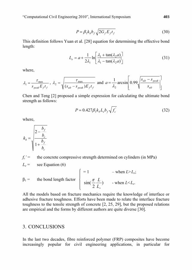
“Computational Civil Engineering 2010”, International Symposium 403
ffffb tEGbkP 21 (30)
This definition follows Yuan et al. [28] equation for determining the effective bond length:
)tan(
)tan(ln
2
1
21
21
1 a
aaLe
(31)
where,
ffpeak tEsmax
1
, ffpeakult tEss )(
max2
and
ult
peakult
s
ssa 99.0arcsin
1
2
Chen and Teng [2] proposed a simple expression for calculating the ultimate bond strength as follows:
'1427.0 cfeb fbLkP (32)
where,
c
f
c
f
b
b
bb
b
k
1
2
fc’ = the concrete compressive strength determined on cylinders (in MPa)
Le = see Equation (6)
= 1 – when L>Le;
)2
sin(eL
L - when L<Le.
β1 = the bond length factor
All the models based on fracture mechanics require the knowledge of interface or adhesive fracture toughness. Efforts have been made to relate the interface fracture toughness to the tensile strength of concrete [2, 25, 29], but the proposed relations are empirical and the forms by different authors are quite diverse [30].
3. CONCLUSIONS
In the last two decades, fibre reinforced polymer (FRP) composites have become increasingly popular for civil engineering applications, in particular for
404 R. Oltean, C. Cozmanciuc, N. Taranu
strengthening of reinforced concrete structures. A wide database of experiments has demonstrated that concrete members strengthened with externally bonded FRP systems are susceptible to failure by FRP debonding, through a variety of mechanisms. For this reason, bond of FRP laminates to concrete has been the subject of numerous experimental tests and theoretical models. All available models for estimating bond strength between FRP laminates and concrete are calibrated to experimental data, although, some of them are based on empirical relations, while others are based on fracture mechanism theories.
References
1. Yao, J., Teng, J. G., Chen, J. F., Experimental study on FRP-to-concrete bonded joints, Composites, Part B, 2005, 36: 99–113.
2. Chen, J. F., Teng, J. G., Anchorage strength models for FRP and steel plates bonded to concrete, Journal of Structural Engineering, 2001, 127(7): 784-791.
3. Pellegrino, C., Tinazzi, D., Modena, C., Experimental Study on Bond Behavior between Concrete and FRP Reinforcement, Journal of Composites for Construction, ASCE, 2008, 12(2): 180 – 189.
4. Oltean, R., Cozmanciuc, C., Munteanu, V., Adhesive Bonding Techniques in Hybrid Structures Made from Fibre REinforced Polzmeric Composites and Concrete, Buletin of the Polytechnic Insitute of Jassy, T. LV (LIX), Fasc. 3, 2009, 85-92.
5. Ganga Rao H. V. S., Taly, N., Vijay, P. V., Reinforced Concrete Design with FRP Composites. CRC Press, Boca Raton, USA, 2007.
6. Hollaway L. C., Teng J. G., Strengthening and Rehabilitation of Civil Infrastructures using Fiber-Reinforced Polymer (FRP) Composites, Woodhead Publishing Limited, Cambridge, England, 2008.
7. American Concrete Institute (ACI), Guide for the design and construction of externally bonded FRP systems for strengthening concrete structures, ACI 440.2R-02, ACI, Farmington Hills, 2002.
8. Féderation International du Béton (fib), Externally bonded FRP reinforcement for RC structures, fib Bulletin 14, fib Task Group 9.3, fib, Lausanne, Switzerland, 2001.
9. Consiglio Nazionale delle Ricerche (CNR), Guide for the design and construction of externally bonded FRP systems for strengthening existing structures: Materials, RC and PC structures, masonry structures, CNR-DT 200/2004, Italian Research Council, Italian Advisory Committee on Technical Recommendations for Construction, CNR, Rome, 2004.
10. Brosens, K., Van Gemert, D., Anchoring stresses between concrete and carbon fiber-reinforced laminates, Proceedings of the 3rd International Symposium on Non-Metallic (FRP) Reinforcement for Concrete Structures, Japan Concrete Institute, Sapporo, Japan, 1997, 1: 271–278.
11. Täljsten, B., Defining anchor lengths of steel and CFRP plates bonded to concrete, Int. J. Adhes. Adhes., 1997, 17(4): 319–327.
12. Bizindavyi, L., Neale, K. W., Transfer lengths and bond strengths for composites bonded to concrete, J. Compos. Constr., 1999, 3(4): 153–160.
13. Maeda, T., Asano, Y., Sato, Y., Ueda, T., Kakuta, Y., A study on bond mechanism of carbon fiber sheet, Proceedings of the 3rd International Symposium on Non-Metallic (FRP) Reinforcement for Concrete Structures, Japan Concrete Institute, Sapporo, Japan, 1997, 1: 279–285.
14. Miller, B., Nanni, A., Bakis, C., Analytical model for CFRP sheets bonded to concrete, Proceedings of the 8th International Structural Faults and Repair Conf., M. C. Forde, ed., Engineering Techniques, Edinburgh, Scotland, U.K, 1999.
15. Neubauer, U., Rostasy, F. S., Bond failure of concrete fiber reinforced polymer plates at inclined cracks—Experiments and fracture mechanics model, Proceedings of the 4th International Symposium on Fiber-Reinforced Polymer Reinforcement for Reinforced Concrete Structures, SP-188, Americal Concrete Institute, Farmington Hills, Mich., 1999, pp. 369–382.
“Computational Civil Engineering 2010”, International Symposium 405
16. De Lorenzis, L., Miller, B., Nanni, A., Bond of fiber reinforced polymer laminates to concrete, ACI Mater. J., 2001, 98(3): 256–264.
17. Nakaba, K., Kanakubo, T., Furuta, T., Yoshizawa, H., Bond behavior between fiber-reinforced polymer laminates and concrete, ACI Struct. J., 2001, 98(3): 359–367.
18. Pellegrino, C., Boschetto, G., Tinazzi, D., Modena, C., Progress on understanding bond behavior in RC elements strengthened with FRP, Proceedings of the International Symposium on Bond Behavior of FRP in Structures, Hong Kong, 2005.
19. Khalifa, A., Gold, W. J., Nanni, A., Abdel Aziz, M. I., Contribution of externally bonded FRP to shear capacity of RC flexural members, J. Compos. Constr., 1998, 2(4): 195–202.
20. Yi, W. H., Kang, D. E., Woo, H. S., Choi, K. S., Yoo, Y. C., Keung- Hwan, K., A study on bond mechanism of fiber-reinforced polymer bonded to concrete, Proceedings of the 2nd fib Congress, Naples, Italy, 2006.
21. a. Lu, X. Z., Teng, J. G., Ye, L. P., Jiang, J. J., Bond–slip models for FRP sheets/plates bonded to concrete, Eng. Struct., 2005, 27: 920–937.
21. b. Lu, X. Z., Teng, J. G., Ye, L. P., Jiang, J. J., Meso-scale finite element model for FRP plates/sheets bonded to concrete, Eng Struct, 2005, 27(4): 564-575.
22. Monti, M., Renzelli, M., Luciani, P., FRP adhesion in uncracked and cracked concrete zones, Proceedings of the 6th International Symposium on FRP Reinforcement for Concrete Structures, FRPRCS-6, World Scientific, Singapore, 2003, pp. 183–192.
23. Savoia, M., Ferracuti, B., Mazzotti, D., Nonlinear bond–slip law for FRP-concrete interface, Proceedings of the 6th International Symposium on FRP Reinforcement for Concrete Structures, FRPRCS-6, World Scientific, Singapore, 2003, pp. 163–172.
24. Holzenkämpfer, P., Ingenieurmodelle des vverbundes geklebter bewehbrung für betonbauteile. Dissertation, TU Braunschweig, 1994. (in German)
25. Neubauer, U., Rostásy, F. S., Design aspects of concrete structures strengthened with externally bonded CFRP plates, Proceedings of 7th International Conference on structural faults and repairs, 1997, 2: 109-118.
26. Täljsten, B., Strengthening of concrete prisms using the plate bonding technique, Internat J Fract, 1996, 82(3): 253-266.
27. Wu, Z. S., Yuan, H., Niu, H. D., Stress transfer and fracture propagation in different kinds of adhesive joints, J Eng Mech, 2002, 128(5): 562-573.
28. Yuan, H., Teng, J. G., Seracino, R., Wu, Z. S., and Yao, J., Full range of FRP-concrete bonded joints, Eng Struct, 2004, 26(5): 553-565.
29. Taranu, N., Oprisan, G., Isopescu, D., Entuc, I., Munteanu, V., Solutii compozite de realizare a structurilor ingineresti, Editura Stef, 2006. (in Romanian)
30. Wu, Y., Zhou, Z., Yamg, Q., Chen, W., On shear bond strength of FRP-concrete structures, Engineering Structures, 2010, 32: 897-905.

“Computational Civil Engineering 2010”, International Symposium Iasi, Romania, May 28, 2010
CAD Software as a Tool in Design
Paul Mutică1, Silivan Moldovan2 and Ioana Moldovan3
1Faculty of Architecture and Urban Planning, Technical University of Cluj-Napoca, Romania 2Faculty of Architecture and Urban Planning, Technical University of Cluj-Napoca, Romania
3Faculty of Civil Engineering, Technical University of Cluj-Napoca, Romania
Summary
The competition among the big producers of software programs is maintained through the evolution of programs that answer any complex problems or the ones that give solutions for any new features needed to be introduced or, often, the creation of large databases that would contain standardized building components. Unfortunately, the designers from different areas are attracted by these new facilities, but they don’t use them at their full potential.
These databases introduced in designing programs together with the new features could be a disadvantage to the professionalism. We must be aware that these programs are tools for drawing and nothing more. They have to ease and help us detail our intellectual work, but not do it for ourselves.
The effect of superficial design of such programs is dangerous and the results, unfortunately, are visible everywhere throughout our country.
This article aims at an awareness that regards what computer aided design should be and not what it has become. Computer, all together with special programs, must be the element throughout the designer explains his project better, which helps him study better solutions and not a tool to design faster, obviously in a more shallow way.
This is the never ending struggle between quantity and quality. Architecture and engineering should not have such problems, the design process is by definition a meticulous process based on intellectual work which should be not be altered by.
KEYWORDS: design, CAD, tool.

“Computational Civil Engineering 2010”, International Symposium 407
1. INTRODUCTION
In the year 2010 the computers are a necessary tool in every field of work. Every office must have at least one. In the construction area the computers are basically the modern tool for design. Engineers and Architects are relying on sophisticated and expensive software to make calculations vital for their fields of work.
The computer is a relatively new tool in the architectural world but is becoming a reliable and indispensable one. In our days there is a multitude of CAD software that offers different kinds of help, based on the field of interest. The CAD software is able to help on matters of mathematical equations to landscape architecture, urban planning and beyond.
The main problem with this kind of software is that the designer has to master the program in order to achieve a good result. It’s very easy to fall on the other side and let the software to control the drafter, but then the result is nothing more than cooking after a recipe, no creativity is involved. The creativity, the utility and viability have to be the main objectives in the design process, the computer is there only for help, to help the drafter to decide certain matters, or to ease the design process and mathematical calculations.
In order to understand such problems it is necessary to understand how the software works, how is programmed to help the user. The paper is referring to one of the first CAD software used in design. At first it was developed just to replace the actual hand drawing but the technology made it to evolve into the 3rd
dimension.
2. CAD – COMPUTER AIDED DRAFTING
CAD – Computer aided drafting is the general term used for the whole range of software used for technical design. They are found in a wide range and specialties:
Automotive and Transportation; Engineering & Construction; Architecture & Urban Planning; Utilities and telecommunications; Education; Manufacturing; Topography; Government database.
They come in different sizes, produced by different software companies and with different database packaging. The most notorious of them all is AutoCAD.

408 S. Moldovan, P. Mutică, I. Moldovan
This program is a myth and the AutoCAD series started as software made for mechanical design, but it has been used also by engineers, architects. In time Autodesk, the company which made these software added databases for other design areas. This is the software that opened new horizons in this field. Initially, such programs offered a simple geometric design based on poly-lines, lines, arcs of circles and curves defined by points. During several years they developed, and more importantly have channeled on specific areas. In our days the CAD software is able to perform from simple 2D drawings to complex 3D virtual models, grouped by materials, layers and textures, each with its own proprieties. Al those CAD software stand at the base of 3D virtual reality and are the key component into building virtual models.
The advantages are very clear. The collaboration between different areas covered in a project can be done faster, easier in a virtual environment that does not put lives in danger and allows the drafter to verify and modify every little aspect for a building. Another advantage is that the software encourages team work allowing more users to design at the same model making the design process for larger projects easier to control and supervise. Each office usually has certain design standards used for projects. These can be implemented in all projects and is not necessary to draw them each time a new project begins. Also encourages team work, exchanging drawings between users being easier and clearer. Those standards can be sent to other collaborators, which can directly implement them in their work file providing a certain graphic look for all the final prints. This file sets the project layout from line type, line scale, line print dimension, drawing scale, print colors, hatches, dimension lines, dimension font, dimension size and units, and many other settings which define the needed graphical approach for the project.
3. VECTORIAL DRAWING
It is imperative that all CAD users know the difference between vector and raster drawings because of the way each type of file format can be used. The vectorial drawing is based on points that contain information and are linked between them. The raster drawing is basically composed from pixels and it is actually a picture.
Both raster and vector images can be manipulated. Because raster images are made of pixels they are easy to stretch, manipulate, change the colors, remove items from it, but you can’t easily change the geometry. For this action you need talent, skills and a steady hand, and most of all a raster drawing has only two dimensions. The raster drawing uses the simplest technique of drawing.
Vector drawings are done in two dimensions and in three dimensions. Vector drawings are actually lines and planes all defined by points called vertexes. Every
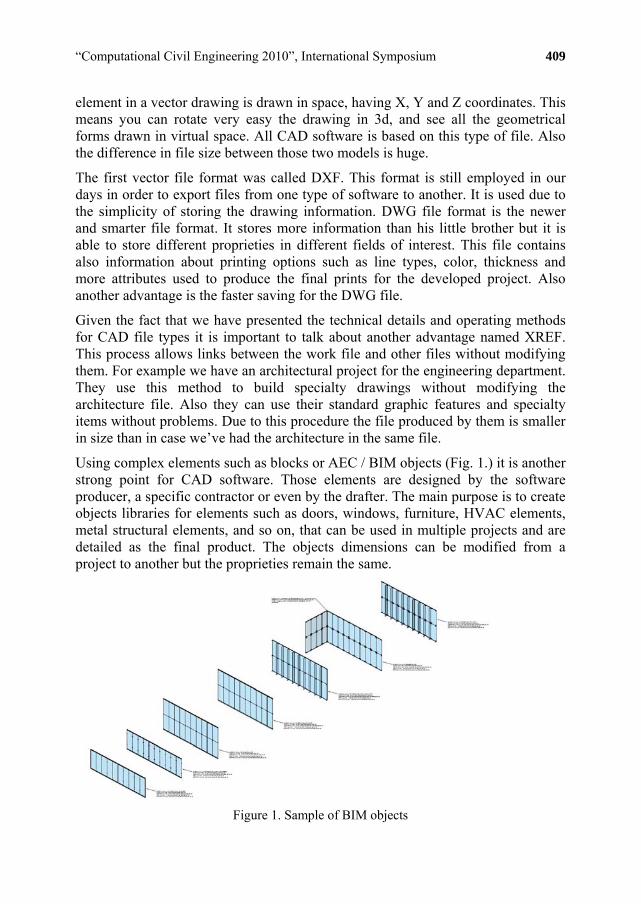
“Computational Civil Engineering 2010”, International Symposium 409
element in a vector drawing is drawn in space, having X, Y and Z coordinates. This means you can rotate very easy the drawing in 3d, and see all the geometrical forms drawn in virtual space. All CAD software is based on this type of file. Also the difference in file size between those two models is huge.
The first vector file format was called DXF. This format is still employed in our days in order to export files from one type of software to another. It is used due to the simplicity of storing the drawing information. DWG file format is the newer and smarter file format. It stores more information than his little brother but it is able to store different proprieties in different fields of interest. This file contains also information about printing options such as line types, color, thickness and more attributes used to produce the final prints for the developed project. Also another advantage is the faster saving for the DWG file.
Given the fact that we have presented the technical details and operating methods for CAD file types it is important to talk about another advantage named XREF. This process allows links between the work file and other files without modifying them. For example we have an architectural project for the engineering department. They use this method to build specialty drawings without modifying the architecture file. Also they can use their standard graphic features and specialty items without problems. Due to this procedure the file produced by them is smaller in size than in case we’ve had the architecture in the same file.
Using complex elements such as blocks or AEC / BIM objects (Fig. 1.) it is another strong point for CAD software. Those elements are designed by the software producer, a specific contractor or even by the drafter. The main purpose is to create objects libraries for elements such as doors, windows, furniture, HVAC elements, metal structural elements, and so on, that can be used in multiple projects and are detailed as the final product. The objects dimensions can be modified from a project to another but the proprieties remain the same.
Figure 1. Sample of BIM objects

410 S. Moldovan, P. Mutică, I. Moldovan
3D modeling is based to a large extent on such information. This way the computer can provide using a model accurately drawn, all the lists of quantities, much closer to reality, saving hours of work if some changes of the solution are required. Unfortunately, in order to build a 3D model correctly, the user must know the project to the smallest detail. This is possible only near the completion of the design process when they have already drawn the final plans. These steps are covered seldom and especially in large, atypical, expensive projects where every technical solution should be checked. The main benefit of designing with computer is that the model could change very easily due to different technical solutions or economical matters and the designer does not have to draw again the whole project. The software is built in a way that allows changes of the drawing scale and line thickness.
There are some directions for this field of use like Wireless technology, Model-based as a 3D model (now being used only as a base for working drawings), full-size virtual buildings that clients may visit, a software payment feature including pay as you use method, and further more. We have deliberately shown the process of how a set of drawings is produced. Certainly, techniques have changed from manual drafting to computer generated drafting or CAD programs, but the process of building construction has not changed. The changes in building construction are not a result of CAD design, but rather from changes in building technology.
4. CONCLUSIONS
The struggle for supremacy between these programs offers us today some complex design programs, but also some exclusivist ones. The most useful approach is that designers from different specialties should work all employing the same program. The disadvantage is appears when one of the specialty designers uses a different CAD program which is not 100% compatible with the one used by the rest of them. Such situations create mismatches between the design or mismatches between different specialties.
Also because of the desire to be the best, CAD software manufacturers are hiring teams of developers to work on the databases that contain the objects employed in the process of design. The bad side is that the majority of those who work for such libraries of objects have no training creativity or design and this can easily be seen because in some cases, working with those objects can be harmful (Fig. 2.). On the other hand, these libraries are designed for large projects, where it is impossible to make a detailed drawing of each component and normally the work is done using typical and characteristic sections, the responsible of the project is

“Computational Civil Engineering 2010”, International Symposium 411
following the project as a whole ensemble. Even if these databases for developing and controlling large projects are good or helpful, they are harmful to young designers, which tend to use them in any project, without entirely controlling its settings. This leads to monotony in the aesthetic details and also to a poor quality of the design process. The attention to detail is overlooked and even forgotten and a good example is that of students from technical universities. The students are founding their skills on these specialized programs, but they are not mastering them, and then they get to the final years with gaps in knowledge from the primary years, which are putting them in difficulty.
Figure 2. 3D model of a building created with objects from the software’s library
The efforts made by the software manufacturers are impressive, but a warning signal need to be set, regarding the quality of the projects designed with these programs. They tend to become increasingly sophisticated in order to meet the needs dictated by our creativity, but also they are more difficult to master, often controlling the designer.
References
1. Abbott, D., AutoCAD: Secrets Every User Should Know Wiley Publishing Inc., ISBN 978-0-0470-10993-9, Indianapolis, 2007.
2. Wakita, O., Linde, R., The Professional Practice of Architectural Working Drawings, John Wiley&Sons, Inc., ISBN: 0-471-39540-4, New York, 2003.
3. Styles, K., Bichard, A., Working Drawings Handbook, Architectural Press, ISBN: 0-7506-6372-3, Oxford, 2004.

“Computational Civil Engineering 2010”, International Symposium Iasi, Romania, May 28, 2010
Studies on Reinforced Concrete Constitutive Laws and Development of a Related Computer Program
PhD Salim Sadi
Department of Reinforced Concrete, Technical University of Civil Engineering, Bucharest, 3872302, Romania
Summary
In order to model structures, especially those made of reinforced concrete, subjected to monotonic or cyclic loadings, two approaches can be implemented, using: A global mode or local model The first one allows describing the behavior of an element (beam, column etc). The law of behavior for this model is represented by the relationship between applied forces and corresponding displacements. The local model examines the behavior of each section of an element or structure taking into account explicitly the behavior of each constitutive material of the element. In our work (or research) several beam and column sections were examined, while diverse parameters were taken into account: the amount of steel, the type of steel grade, the dimensions of the section, the concrete strength , etc. The main aim of this work is to study the various laws of behavior and to quantify the contribution of the factors that influence the behavior of the section. In the first part of our work, we study material behavior, and then we develop detailed studies on the behavior of the front section so that we could trace the moment-curvature. During this part, the calculations will be made by a program in visual basic format (Microsoft Visual Basic 2008 ”P.C.C.S.E”). On the one hand, this program has enabled us to simplify the task, on the other hand, to improve our knowledge in the field of software
KEYWORDS: concrete, reinforced, steel,
1. INTRODUCTION
In order to model structures, especially those made of reinforced concrete, subjected to monotonic or cyclic loadings, two approaches can be implemented, using:
- A global model - A local model
Studies on Reinforced Concrete Constitutive Laws 413
The first one allows describing the behavior of an element (beam, column etc). The law of behavior for this model is represented by the relationship between applied forces and corresponding displacements.
The local model examines the behavior of each section of an element or structure taking into account explicitly the behavior of each constitutive material of the element.
2. OBJECTIVE OF THE STUDY
In the author’s work several beam and column sections were examined, while diverse parameters were taken into account: the amount of steel, the type of steel grade, the dimensions of the section, the concrete strength , etc.
The main aim of this work is to study the various laws of behavior and to quantify the contribution of the factors that influence the behavior of the section.
In the first part of the work, a study of the material behavior was done, and it was developed a detailed study on the behavior of the front section so that the moment-curvature could be traced.
During this part, the calculations were made by a program in visual basic format (Microsoft Visual Basic 2008 “P.C.C.S.E”).
On the one hand, this program has enabled the author to simplify the task and on the other hand, to improve the knowledge in the field of software applications.
3. CONSTITUTIVE LAWS FOR REINFORCED CONCRETE COMPONENTS
3.1. Characteristics of Materials
The purpose of this section is to present the main characteristics of materials used in reinforced concrete, then the models adopted for conducting the calculations.
3.1.1. Concrete
The compressive strength of concrete is determined either by 140 mm cubic test tube, either by 160 mm diameter by 320mm high test cylinders (common in Algeria).

414 S. Sadi
cf
For this specimen, the two end faces or planes must be rectified and perpendicular to the axis of the cylinder body. Poor preparation of the test tube influences the value of that we are seeking for.
Many researchers are interested in defining the concrete laws of behavior. We are presenting below a few proposals for such laws.
3.1.2 Behavior Laws Proposed by Cusson and Paultre
The stress-strain curve proposed by Cusson and Paultre is shown in Figure.3.1
Fig.3.1 - Axial deformation of concrete (Daniel Morgean 1996).
ccckccc
ccccc k
kff
,)/(1
)/(
)/( ccccc
c
fE
Ek
Where cf and c are respectively the stress and strain in concrete, and Ec is the
modulus of concrete, the k factor controls the slope.
There are dozens of behavior laws. For our research, we used the behavior law that is proposed by Vecchio and Collin. The Mathematical expression is:

Studies on Reinforced Concrete Constitutive Laws 415
cb
b
b
bb R
2
00
2
0bb0
cb R bubb 0
Fig.3.2 - Simplified Relationship for Stress-strain Curve (Vecchio and Collins)
The curve proposed by Vecchio and Collins consists of two parts: the bottom (a second degree curve until a strain that equals 2 ‰) and a plateau (up to a strain that equals 3.5 ‰).
3.1.3. Reinforcing Steel
Figure 3.3 is a diagram obtained in a tensile test on a specimen of steel apparent diameter of 18.5 mm. (Oliver Germain, 2006).
3.5‰ 2‰
Rc
bc

416 S. Sadi
Fig.3.3 - Force Deformation Diagram (Oliver Germain, 2006)
Depending on the needs, the analysis uses:
Idealization faithfully representing the general curve shape of the tensile test as in Figure 3.3, or the idealization of this curve by a simple law, “elasto-plastic” deformation limit, as in Figure 3.4.
Fig. 3.4 - Representations of the Law "elastoplastic" (Oliver Germain, 2006)
In this part of the work there was presented a literature review on the behavior of concrete and steel.
By reading the foregoing, one notices that there are differences between laws. It is very difficult to use certain laws, given the number of trials whose parameters must
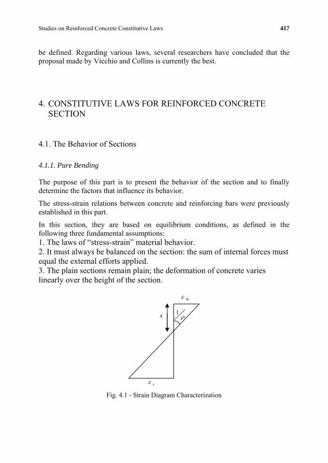
Studies on Reinforced Concrete Constitutive Laws 417
be defined. Regarding various laws, several researchers have concluded that the proposal made by Vicchio and Collins is currently the best.
4. CONSTITUTIVE LAWS FOR REINFORCED CONCRETE SECTION
4.1. The Behavior of Sections
4.1.1. Pure Bending
The purpose of this part is to present the behavior of the section and to finally determine the factors that influence its behavior.
The stress-strain relations between concrete and reinforcing bars were previously established in this part.
In this section, they are based on equilibrium conditions, as defined in the following three fundamental assumptions: 1. The laws of “stress-strain” material behavior. 2. It must always be balanced on the section: the sum of internal forces must equal the external efforts applied. 3. The plain sections remain plain; the deformation of concrete varies linearly over the height of the section.
bc
x 1
s
Fig. 4.1 - Strain Diagram Characterization

418 S. Sadi
The data of the problem in the first case are P , b, and h0 and the unknown is the As section reinforcement. In the second case, P , b, h0 are fixed and the unknown are the values of As and As'. In the third case, the steel mark was changed to check if it influences the behavior of the section.
In the fourth case, there were established P , As, b and the unknown is the value of h0. In the end, there were made some variations of the FC28 concrete resistance value.
In order to draw diagrams of the curve, there were followed the steps below: - Discretization-section: this step aims to refine the accuracy of the numerical
integration of the stress distribution; - The defining of the laws of material behavior. For this problem there was
chosen the parable chart – rectangle for concrete and elasto – plastic model for steel;
- Choosing the number of steps and we fix the value of deformation:
nibc
35,0.
- Choosing a value of x;
0 dA
- Calculation of the specific deformations using the characteristic curve for concrete and steel;
- The check of the equation of equilibrium:
This equation allows the author to check the position of the neutral axis; if the result of the equation of equilibrium is close to 0, it can be concluded that the chosen x value is correct and if the equilibrium condition does not resist, another value of x must be introduced and the process is repeated until the value of x that satisfies the equation is found.
- The calculation of the value of the curvature
00
1hahx
ia
ibc
ia
ibc
- The calculation of the corresponding bending moment
dAM i ..
- Repeating the same steps up to the last one, noted as «n».
Through the present research, the author developed a computer program in visual basic training Microsoft Visual Basic 2008 “P.C.C.S.E” which allowed him to ease the task of calculation.
They represented all stages of calculation in the form of a flowchart.

Studies on Reinforced Concrete Constitutive Laws 419
4.1.2 The Flowchart
Fig 4.2 The P.C.C.S.E Program Designed by: PhD Salim Sadi, Supervisor: Prof. Univ. Dr. Ing.: Liviu CRAINIC

420 S. Sadi
Fig 4.3 - The P.C.C.S.E Program designed by: PhD Salim SADI, Supervisor: Prof. Univ.
Dr. Ing. Liviu CRAINIC
H: Total height of a reinforced concrete section.
B: Transversal dimension (width or thickness of a section).
D: Distance from the centroid of tensile reinforcement to the most extremely compressed fiber.
d’: Distance from the centroid of compressed reinforced fiber to the most compressed extreme fiber.
f’’c : Resistance of concrete to compression.
Es : Module of steel elasticity.
fS : Tensile stress in steel.
next: The normal axial force) in the section.
n: The number of steps.
r: Distance between two discretizations.

Studies on Reinforced Concrete Constitutive Laws 421
4.1.3. Example of application
The purpose of this example is to draw the diagram of the moment-curvature for the section and to see the factors that influenced the behavior of the section of the element.
Fig.4.4 - Moment-curvature diagram superposition for diverse steel amounts; Fe400
Fig.4.5 - Moment-curvature diagram superposition for diverse steel amounts; Fe400.
PFor a reinforced section in the lower part and from Fig.4.4 shows that: 1) For = 0.5 ℅ there was a long plateau, therefore the post-elastic deformations in the section are very important.

422 S. Sadi
Increasing the moment of the section is due to increased “X” branch leverage. 2) For = 2 ℅ we see that P /1 has decreased in value by 50 % as compared to P = 0.5 ℅. The more " P " is increasing, the less /1 is increasing, which means that the section just less ductile. 3) For a section with upper reinforced Fig.4.5, there can be noted that the moments are very important due to the increased leverage and the section becomes less ductile as compared to a simply reinforced section.
We note that in a reinforced concrete section, steel plays a very important role. The more P decreases, the more ductile the section becomes, so the post elastic deformations for a section of concrete are important.
Fig.4.6 - Moment-curvature diagram superposition for diverse steel amounts; Fe400
Fig.4.7 - Moment-curvature diagram superposition for diverse steel amounts; Fe400 and
Fe500.

Studies on Reinforced Concrete Constitutive Laws 423
In the third case, there can be noticed in Fig 4.7 that the nuance of steel has great importance on the ductility of the section and on calculations. It was found that for a section with P = 0.5 ℅, Fe500 steel grade has less ductility than Fe400 steel. So, for a section of reinforced concrete, a section with Fe400 steel is preferably used rather than a Fe500 section, for better energy dissipation.
The nonlinear regression “adjustment curve”
For Fe500
Fig.4.8-Adjustment curve
For Fe400
Fig.4.9- Adjustment curve

424 S. Sadi
The graphs represent the diagrams at the bending moment for the steel Fe500 and Fe400. The objective of this part is to find an equation that will be close to the one used by the visual basic program, to notice the non-linear regression “adjustment curve” and the percentage of errors. After the graphs, less than “5 ℅” errors have been found.
In the fourth case, P is fixed, it equals 0.5 ℅; and b = 30cm, the unknown element of the problem is the h0 utility value.
The purpose of this part is to check the influence of the effective height behavior of the section.
Fig.4.10 - Moment-curvature diagram superposition for different heights
After Fig.4.10, there can be noticed that h0 is higher as the moment is longer.
For h0 = 15.36 cm, /1 was equal to 0.15 rad, and for h0 = 60cm, /1 was equal to 0.135 rad. It is obvious that the smaller the angle, the longer the moment, and the section become less ductile.
If we calculate the ductility factor between the two, we find a percentage of 25 ℅.
In the fifth case, the author focused on the strength of the concrete influence on the behavior of the section.
In the fifth case, in Fig.4.11 there is a small variation of /1 for a section with a FC28 concrete strength equal to 15MPa, and a section with a FC28 concrete strength equal to 30MPa.
It was reached the conclusion that increased resistance leads to increased ductility. This is why the codes that call for increasing column concrete strength requested by the normal efforts are more important.
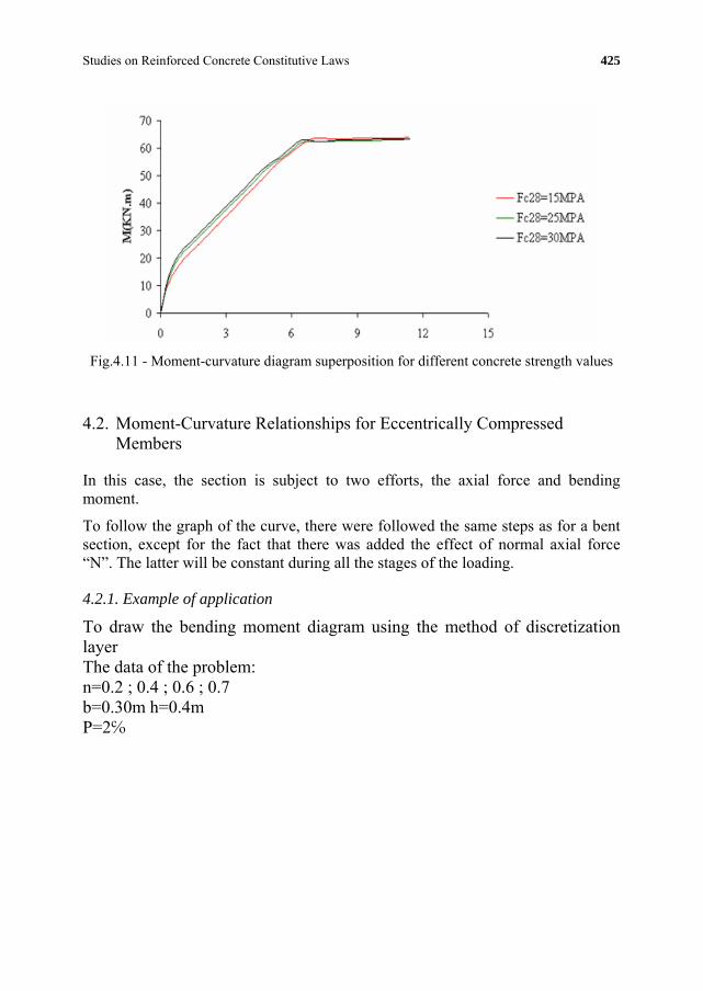
Studies on Reinforced Concrete Constitutive Laws 425
Fig.4.11 - Moment-curvature diagram superposition for different concrete strength values
4.2. Moment-Curvature Relationships for Eccentrically Compressed Members
In this case, the section is subject to two efforts, the axial force and bending moment.
To follow the graph of the curve, there were followed the same steps as for a bent section, except for the fact that there was added the effect of normal axial force “N”. The latter will be constant during all the stages of the loading.
4.2.1. Example of application
To draw the bending moment diagram using the method of discretization layer The data of the problem: n=0.2 ; 0.4 ; 0.6 ; 0.7 b=0.30m h=0.4m P=2℅

426 S. Sadi
Fig 4.12 - P.C.C.S.E Program designed by: PhD Salim SADI, Supervisor:
Prof.Univ.Dr.Ing.
n=0.8 n=0.6
n=0.4
n=0.2
)(1 rad
Fig. 4.13 - Moment-curvature diagram, different for axial force

Studies on Reinforced Concrete Constitutive Laws 427
The author found that: Increasing the axial load applied on the section of the column leads to a decrease of ductility. According to Figure 4.13, it is showed that:
1.For n = 0.2 the section has a ductile behavior, i.e. it behaves like a bent section; 2.For n = 0.4 the section has a semi-ductile behavior. Since that post-elastic deformation has the effect of decreasing, the “n” must reinforce this section with transversal reinforced frames and a 10 cm spacing to confine the concrete section; 3.For n = 0.8 it presents a brittle failure.
5. CONCLUSION
The author noted that the law of moment curvature will provide a picture of the phenomena developed in a section of reinforced concrete.
Since then, there was deterioration in the stiffness and the post-elastic deformations are large. It was noted that the increased moment in the section after the start of the discharge was due to the increased leverage. So the smaller X is, the more the
1
angle increases. There can be seen that the post-elastic field is the effect of the steel yielding.
According to a little comparison between diverse amounts of reinforcement, it was discovered that the greater the amount of steel, the more fragile the section becomes.
It was also noticed that the steel grade is extremely important for the ductility of the section. During calculations, we found that for a section with P = 0.5 ℅ and the Fe500 steel grade, ductility was less important than for the Fe400 steel. So, for a reinforced concrete section, Fe400 steel is preferably used rather than Fe500 sections - for better energy dissipation.
Regarding the section of the column, we can mention that:
If the axial force is more than ‘n’, the general section becomes fragile and in the Fig 4.13, there can be seen that for n = 0.2, the behavior of the section is similar to the bent ductile sections.
A brittle fracture occurs, including concrete crush, rather than steel yielding. Increasing the axial force thus leads to lower ductility of columns.
The axial force is important. The corresponding cracking and yielding moments are naturally elevated beyond a certain value of "n".

428 S. Sadi
In short, there are diverse possible types of analysis that can be used to quantify the influence of various parameters on the local behavior of an upper reinforced beam or column.
The previous examples provided a general view on how the sections of a reinforced concrete element behaved, and they allowed the author to improve his understanding regarding the phenomena that occur in the component parts of the structure.
References:
1.Crainic, L., Reinforced Concrete Structures, Napoca Star, 2003. 2.Crainic, L., Calcul Post-Elastique des Structures, MatrixRom, 2000. 3.Pacu, R., Béton Armé, MatrixRom, 2000. 4.Mohamed, A. A., Auto Teaching Of Yeses Use « Visual Basic 6.0».Autto Yuse. 2007 . 5. Gilmore J., Datafit. Oakdale.2007. 6.Muno, C., Bien Implémenter un Projet Avec Visual Basic6,2004. 7.Sadi, S., Programme P.C.C.S.E « Visual basic.2008 »,Bucharest.2010.

“Computational Civil Engineering 2010”, International Symposium Iasi, Romania, May 28, 2010
Comparative analysis regarding settlement prediction founded on collapsible soils
Stanciu A1, Iliesi A. T.1, Lungu I.1 1Department of Roads, Railways, Bridges, and Foundations, Technical University “Gheorghe
Asachi”, Iasi, 700050, Romania
Summary
Collapsible soils are soils sensitive to moistening, displaying a special behavior that results from the supplementary settlement due to the partial or total moistening of the soil subjected to the geological stress and/or while in service.
The settlement evaluation develops in a complex calculation that should consider both the initial conditions regarding the moisture content and the load conditions during constructions service, all related to the soil nature and thickness within the active zone of the foundation.
Computational approach and diagrams are displayed concerning the total settlement based on the deformations zones correlated with soil properties related to setting collapsible soils by careful assessment of geotechnical parameters, design principles and rules in the European context.
This paper presents a case study of a continuous foundation on loessy silty clay with interpretations and concluding remarks on the settlement value obtained by calculation using Romanian regulations and Eurocode 7.
The main issue addressed in the settlement prediction is related to the soil parameter assessment considering safety factors applied to laboratory test results.
Stress-strain curves obtained from undisturbed soil samples may have the partial safety factors applied to each point of the experimental curve, resulting thus in a range of curve display for both the natural and saturated soil condition.
Case studies are generally useful for evaluation of the building safety founded on different categories of collapsible soils, the present study reflecting this specific behaviour.
KEYWORDS: collapsible soils, settlement, prediction, active zone
1. INTRODUCTION
Collapsible soils are defined as macroporous cohesive soils, with granulometric
composition including silt between porosity and a
saturation degree when in natural condition [1], [2].

430 Anghel S., Iliesi A-T., Lungu I.
Settlement represents a coherent expression of the stress and deformations state due to the loads during service that in case of collapsible soils develops to a very large extent as induced degradations of the following nature:
Architectural cracks in brick masonry panels, slabs, finishing or tilting of the rigid structure (retaining walls, cooling towers, communication towers, etc.);
Structural cracks which are located in structural elements (columns, beams, masonries), because of different settlements, that can generate structure and building collapse, due to column buckling , the appearance of plastic hinges in beams, the displacement and failure of the load bearing masonry;
Combined occurrence, with an architectural aspect and structural tendency, like cracks in the slabs, beams, shear walls, jamming of the windows and doors, pipe dislocation, offsetting of the machines, etc.
The absolute settling of the foundation is determined using a staged determination based on the summing of the individual settlement elementary layers method in accordance to (3),(4),(5) thus determining the settling under the action of the external loads transmitted by the building on the footing of the foundations, and the supplementary settlement which may appear in the same emplacement conditions, but with the ground totally flooded (saturated condition). Using this calculation method, the soil under the footing is divided in elementary layers down to the active zone, having the thickness comprised between the following limits
.
The necessary data for the calculation of the settlement is determined through laboratory testing, performed on undisturbed soil samples.
The soil deformation modulus used for the calculation of the soil settlement is determined based on the experimental values obtained after the laboratory results (oedometer/triaxial tests) are processed (figure 1).
The soil modulus (E) is evaluated based on the design value of the oedometric deformation modulus (Eoed) for the given layer, determined in the pressure interval comprised between the geologic pressure ( ) and the medium pressure which
appears in the compressed layer when foundation is in service . The oedometric modulus is multiplied with the correction coefficient corresponding to the physical soil parameters of the given layer condition (4), (6), (7).
Due to the fact that these soils settle differently in case of flooding, separation of soils in categories such as group A, which at moistening under geological pressure
present supplementary settlements smaller than 5 cm and group B,
which present settlements bigger or equal to 5 cm . While evaluating

“Computational Civil Engineering 2010”, International Symposium 431
the supplementary settlement at moistening when soil is subjected only to
geological pressure , it is verified if the structural pressure of the collapsible soil , has values bigger than the geological pressure itself. When this is the case, the supplementary settlement of each elementary soil layer due to moistening is computed with the following formula:
[1]
otherwise, the general relationship remains:
[2]
where represents the strain values for the saturated, respectively the natural soil condition, extracted from the stress-strain curves in figure 1.
Figure 1. Typical stress-strain curve from oedometer tests on collapsible soils
2. SETTLEMENT PREDICTION FOR CONSTRUCTIONS ON UNSATURATED COLLAPSIBLE SOILS
The total settlement (S) consists of the sum from the settlement considering the natural/unsaturated soil condition (Sn), the supplementary settlement due to moistening (Im), either for group A or group B soil category as in the following relationships:
(group A) [3]
(group B) [4]

432 Anghel S., Iliesi A-T., Lungu I.
where is the supplementary settlement due to moistening when soil is subjected only to the geological pressure and represents the supplementary settlement due to moistening when soil is subjected only to the net pressure during service
The supplementary settlement due to moistening generated under geological pressure is assessed on the entire thickness of the collapsible soil based on the relationship:
[5]
where n – number of the elementary soil layers; – the thickness of the elementary soil layers; m – coefficient of the working conditions,representing the difference between the theoretical and experiemental value, which can be also regarded as a safety factor, usually m=1 when lacking experimental results; – the supplementary settlement for each elementary soil layer, computed based on relationships (1), (2), depending on the soil category (group A or B) with values extracted from the double oedometer procedure.
Supplementary settlement due to moistening under the loading transmitted by the shallow foundation (Imp) is computed at the foundation level Df for all the deformation zones in the soil with the following relation:
[6]
n - the number of elementary layers in the active zone; –the thickness of the elementary soil layers of order i (m); m –coefficient of the working conditions;
–foundation depth; – the specific supplementary settlement due to the moistening of the elementary soil layer when in service. It is obtained based on the results from the double oedometer tests with the relation:
[7]
where: –specific deformation of the saturated/flooded soil, for ;
– specific deformation of the saturated/flooded soil, under the geological stress ; –the geological stress computed with the unit weight of the saturated soil ; -the vertical stress from the shallow foundation loading (pnet) at the
middle of the elementary soil layer, according to (3).
The estimation of the total probable supplementary settlements due to moistening (S ) [8], is realized for the deformable soil zones counting on the

“Computational Civil Engineering 2010”, International Symposium 433
structural pressure . Thus, the superior deformable area (zone I) extends to the depth at which the vertical unit stress as the sum of the stress induced by the
shallow foundation load and the self weight of the soil is greater and becomes equal to (Fig. 2).
It is also the case that soil layers sensitive to moistening, generate supplementary settlements too at the base level, called inferior deformable aria (zone III). The
geological pressure in this zone is big enough so that the total vertical stress becomes again greater than . In the following graph (Fig. 2), between the
two deformable zones (I and III) an inert zone (zone II) is encountered, because in this area the total vertical stress is smaller than and there are no supplementary settlements due to moistening.
Fig. 2. Characteristic zones in the foundation soil consisting of collapsible soils: I –
superior deformable area; II inert area; III – inferior deformable area
Interpretations related to the development of the active zones correlate the foundation width B, the value of the net pressure , the thickness H of the layer sensitive to moistening and the value of the structural pressure and define the collapsible soil behaviour according to group A or B as it follows (Fig. 3a ... e):
For group A of collapsible soils, the following cases can develop:
when the width of the foundation is large, the transmitted pressure and the thickness of the collapsible soil layer are small there is present only the superior deformable area (zone I);

434 Anghel S., Iliesi A-T., Lungu I.
when the width of the foundation is small, the transmitted pressure from the reduced foundation and the thickness of the collapsible soil layer are large, only the inert aria (aria II) can appear.
For group B of collapsible soils the following cases can appear:
when the soil pressure and the width of the foundation are large only the superior and inferior deformable areas (zone I and III) can develop;
Fig.3. Characteristic situations for foundation soils consisting of collapsible soils
when the width of the loading surface (footing) is reduced and the transmitted net pressure is small there is only zones II and III;
when the foundation width and value of the net pressure are large there is only zone I.
3. CASE STUDY AND INTERPRETATION OF THE SETTLEMENT PREDICTION
The case study intents to develop a specific condition for supplementary settlement evaluation related to an individual footing on loessy silty clay. During soil

“Computational Civil Engineering 2010”, International Symposium 435
Fig
ure
4. S
ettle
men
t dia
gram
s re
sulte
d fr
om th
e se
ttlem
ent a
naly
sis
of th
e ca
se s
tudy
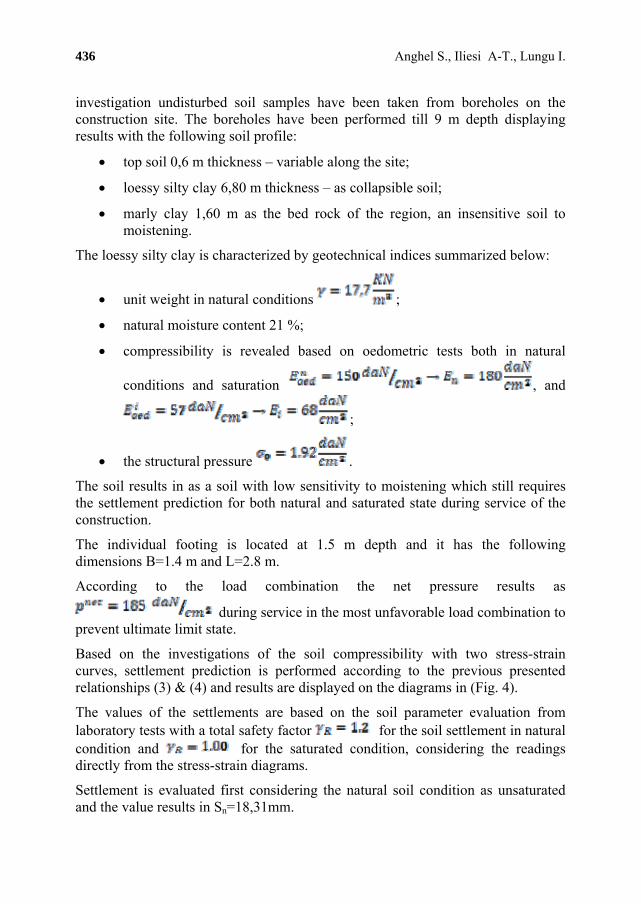
436 Anghel S., Iliesi A-T., Lungu I.
investigation undisturbed soil samples have been taken from boreholes on the construction site. The boreholes have been performed till 9 m depth displaying results with the following soil profile:
top soil 0,6 m thickness – variable along the site;
loessy silty clay 6,80 m thickness – as collapsible soil;
marly clay 1,60 m as the bed rock of the region, an insensitive soil to moistening.
The loessy silty clay is characterized by geotechnical indices summarized below:
unit weight in natural conditions ;
natural moisture content 21 %;
compressibility is revealed based on oedometric tests both in natural
conditions and saturation , and
;
the structural pressure .
The soil results in as a soil with low sensitivity to moistening which still requires the settlement prediction for both natural and saturated state during service of the construction.
The individual footing is located at 1.5 m depth and it has the following dimensions B=1.4 m and L=2.8 m.
According to the load combination the net pressure results as
during service in the most unfavorable load combination to prevent ultimate limit state.
Based on the investigations of the soil compressibility with two stress-strain curves, settlement prediction is performed according to the previous presented relationships (3) & (4) and results are displayed on the diagrams in (Fig. 4).
The values of the settlements are based on the soil parameter evaluation from laboratory tests with a total safety factor for the soil settlement in natural condition and for the saturated condition, considering the readings directly from the stress-strain diagrams.
Settlement is evaluated first considering the natural soil condition as unsaturated and the value results in Sn=18,31mm.

“Computational Civil Engineering 2010”, International Symposium 437
As by consequence of water infiltration into the soil, a supplementary settlement is anticipated with different values, depending on the group category of the collapsible soil.
When evaluating the supplementary settlement under the geological pressure, the
value of the structural pressure of the soil is influencing the resulted value of Img, based on the two relationships possible for img value (1) and
(2). Applying relationship (2) because , the resulted Img=62,10mm refers
the collapsible soil as fitting the group B since .
The supplementary settlement under service, Imp results in 13.15mm, which also creates a total supplementary settlement Im(group B)=75,25 mm.
The final settlement as predicted in case of total saturation of the soil beneath the foundation is the sum of all the values mentioned above S(group B)=93,52 mm. The deformation zones develops in particular to this situation only as zone I and II, zone III is not developed when correlated to the high structural pressure σ0.
In case the collapsible soil displays a lower structural pressure, , the supplementary settlement can reduce to less than 5 cm, changing the soil group B to group A, for which only supplementary settlement under service remains relevant and consequently Im(group A)=13,15 mm and S(group A)=31,42 mm.
When saturation of the same collapsible soil may happen before construction is built then the only settlement is the one based on the prediction of the saturated stress-strain curve with the value Si=47,59mm, which is higher than when including the soil to group A and developing the supplementary settlement due to total flooding/saturation after the construction is built.
4. CONCLUSIONS
Saturation of collapsible soils induces supplementary settlements compared to the initial unsaturated state and consequently settlement prediction is required for all future situations that may happen and endanger the construction.
When the collapsible soil develops a high structural pressure σ0 the supplementary settlement is significantly reduced under service and this effect may be furthered by compacting the soil previous to construction.
When changing from the previous design codes to Eurocodes, the safety factor approach is changed from the unique value, to various values applied to soil properties or on soil parameters.

438 Anghel S., Iliesi A-T., Lungu I.
In case of settlement prediction of collapsible soils the partial safety factors as γR should be applied on increasing the strain values of all experimental points on the stress-strain diagram, shifting the curvature downwards and thus increasing the supplementary settlement due to moistening.
There is no specificity yet suggested as to the extent of the partial safety factor value in this particular situation that needs further investigations to conclude over the effect of the settlement prediction in correlation to the protection measures necessary to reduce the differential settlement effect.
References
1. Stanciu, A., Lungu, I. – Fundații. Editura Tehnică, București, 2006 2. Lungu, Irina; Stanciu, A.; Boți, N. – Probleme speciale de Geotehnică și Fundații, Editura
Junimea, Iași, 2002 3. NP 112/2004, Normativ pentru proiectarea structurilor de fundare directă, 4. STAS 3300/2-85, Calculul terenului de fundare in cazul fundarii directe, 5. P7/2000, Normativ privind fundarea constructiilor pe pamanturi sensibile la umezire (Proiectare,
Executie, Exploatare), 6. SR EN 1997-1:2004 Eurocod 7 – Proiectare geotehnică. Partea 1: Reguli generale, 7. SR EN 1997-2:2008 Eurocod 7- Proiectare geotehnică. Partea 2: Investigarea și cercetarea
terenului 8. Robert W. Day, Foundation Engineering Handbook: Design and Construction with the 2006
International building code, The McGraw-Hill Companies, 2006 9. Kezdi, A. - Handbook of soil mechanics, vol.I, Akadémiai Kiadó, Budapesta, 1974 10. Costet, J., Sanglerat, G.- Cours pratique de mécanique des sols, DUNOD - Paris, 1969 11. Yuan, Z.X., Wang, L.M.- Collapsibility and seismic settlement of loess, China, 2007

“Computational Civil Engineering 2010”, International Symposium Iasi, Romania, May 28, 2010
Comparative analysis of structural response to various methods of calculation for reinforced concrete frame structures
Ţepeș Onea Florin1, Gelmambet Sunai1
1Faculty of Construction, University Ovidius , Constantza, 8700,Romania
Summary
The paper proposes determine for the framed structures, the level seism forces, for which, the frame passes from static undetermined frame in mechanism because of the graduated forming of plastic articulations.
Although, these seismic forces can be comparate with the seismic static equivalences forces that result from the current design.
So, we can determinate both the reserve of resistant of the framed structures through of the plastic reinforcement and the pursuit of the areas where can be appeared the plastic articulations or when the concrete points have the limit of pressure. The structures analyzed are from reinforced concrete. The project proposes determine the tension fact both of the concrete and the reinforcement, too.
For this, use the finite elements for concrete and others for the stretched reinforcement and pressed reinforcement, too.
For the determination the tension state of the finite elements can be done using nonlinear elements to model the reinforcement after exceed the limit of elasticity way. For the determination the seismic force S and this distribution of the horizontal and vertical structure of resistant can be done on normative P100, its combination with the others charges categories can be done on STAS 10101/0A, and the dimension of reinforcement can be done on STAS 10107/90. For the determination the efforts can be used comparatively both the equivalent static force method (using at much more simple structures with reduce relative high) and the method of time integration (at higher and more complex buildings where the effect superior vibration is much more important).
The level calculus seismic forces supposed the appearance of the plastic area in the structure resistance at the maxim earthquake anticipated by the prescriptions. It’s going to identify the location of plastic articulations and the level of inelastic deformation produced by the seismic action. These aspects are going to be touch by the working content.
KEYWORDS: reinforced concrete, mesh, static equivalent forces, plastically articulations

440 F.Ţepeș, G. Sunai
1. STRUCTURES IN POST-ELASTIC ANALYSIS OF REINFORCED CONCRETE FRAMES.EXAMPLE 1
This theme aims to determine the structure within, the seismic forces for which the structure changes from multiple structure statically indeterminate stage in the gradual formation of the joint mechanism of plastic.
A solution obtained by finite element method, regardless of the problem studied is an approximate solution.
Mesh structure and the change is real unknown function (movement) is replaced with local variations, the field elements according to nodal values. Convergence is achieved only if the approximation functions satisfy certain conditions.
Types of analysis used in this study:
1. Beam type finite elements, equivalent static seismic forces.
2. Quadrilateral elements mesh for concrete reinforcement and Truss (with mesh restoration for modeling concrete stretching area .
In the first case study (case 1), the structure was analyzed in finite element mesh type beam. Load the structure's weight and the equivalent static seismic forces will result in bending moments at each end of beam. Analysis of the first case was the normal load and earthquake in the direction y. For this study, obtained the following values for the maximum horizontal and vertical displacements:
Tabelul 1 (case1): Dymax 0.419E-2m Dzmax 0.649E-3
So that, the maximum bending moment for beams was 93.54 KNm, and for the beams having 25x40cm2 section, we obtained an armed area of 9.42 cm2.
The second case study (case 2) corresponds to a mesh to shape the concrete by means of quadrilateral finite elements with 8 nodes and reinforcement by Truss elements.
If the solution was chosen quadrilateral elements with 8 nodes per element so that bending can be well modeled as these elements allow the expression of movement through non-linear functions and voltage per cell by linear functions. Also for better accuracy of the calculation level is used 4 numerical integration. Case study chosen for loading on beams is 44KN / m. Practically previous studies have shown that even a coarse mesh using these elements for modeling the bndings involves an error to the exact solution up to 20%.
Seismic forces were applied in the form of equivalent static forces distributed beam nodes and the size is 7% by weight.

“Computational Civil Engineering 2010”, International Symposium 441
The reinforcement percents for columns are 1.1% and for beams 0.94%. The values of reinforcement areas were obtained from bending moments in the first study.
In the first step of calculus at these loads it obtained a maxim unitary effort of compression in concrete by 7.7 N/mm2 (for columns). It can be compared this unitary effort by the bottom of the central column with the unitary effort obtained in the same section from the analyze with beam elements(the first case):
N M
A W
and it obtains: 2 228.4 406311 444 6755 / 6.7 /
0.0045 0.09KN m N mm
For the reinforcements the maximum unitary stress are 45.7 N/mm2.
Fig.1 a) The area where the stretch unitary efforts passed over maxim value admit in the first step calculus. b) remake of mesh
Tabel 2 (case 2): Maximum displacements (m)
Unitary stress for columns N/mm2
Unitary stress for beam N/mm2
Unitary stress for reinforcement N/mm2
Dymax=0.27E-2 σ(+)=4.0 σ(+)=5.3 σ(-)=45.7
Dzmaz=0.117E-2 σ(-)=7.7 σ(-)=5.4
It can observe that the frame has still a wide capacity reserve until the entrance flow, but the concrete touches 61% from maxim compression limit.
For modeling the concrete crack it remakes the mesh in the areas where appears the stretched efforts much more than 1.25 N/mm2. We can see that in fig.1. This reshape can be done by taking off the stretched concrete area and keeping the frame. Doing that it can observe the concrete crack for all area field beams, on the side of the stretched fiber and the crack concrete at the bottom of the columns (fig.2).

442 F.Ţepeș, G. Sunai
The maximum displacements up with an low percent and the maximum unitary stress for pillar lows from 7.7 N/mm2 to 6.9N/mm2 in the case of compression and the stretching from 4.0 N/mm2 to 2.8 N/mm2. This happened accordingly of redistribution effort state.
Fig.2 The areas where the unitary effort stretched are over the maxim admit value of the 2
step calculus. (the third case)
The following analyze is about the concrete elimination in the areas where the stretched maxim values are over 1.25 N/m2. These points are presented in fig.2.
The maximum values of displacements are presented bellow:
Tabel 3 (case 3) Maximum displacements (m)
Unitary stress for columns N/mm2
Unitary stress for beam N/mm2
Unitary stress for reinforcement N/mm2
Dymax=0.31E-2 σ(+)=2.8 σ(+)=3.4 σ (+)=49.5
Dzmaz=0.137E-2 σ(-)=6.9 σ(-)=6.6
It can be observed that for the same level of seism static equivalent forces, accordingly of the efforts redistribution, after the eliminate of the stretched area, aren’t the major modifications of the maxim unitary effort at the compression. At the stretching maxim unitary effort in the columns, the maxim values are under 1.8 N/mm2.
The following analyze have a constant gradually of the level seism forces, reaching the maxim limit in concrete for an amplification factor of these forces equal with 2. For this level these forces equal with 2. For this level of seismically static equivalent forces, the maxim tensions in the frame are at a minim value under 150 N/mm2.
In the 4 th case the seism action isn’t represented (introduced) like seism static equivalent forces, such as an accelerograme, practicaly used time integration. The

“Computational Civil Engineering 2010”, International Symposium 443
seism exciting is introduced by an scaled accelerograme at 0.2g. Time step is 0.02s and the all accelerograme time is 15.98s.
Because aren’t major modifications of the unitary efforts distribution when we introduce in analyze the crack in concrete stretching areas, the analyses for time integration aren’t considerated in this case. For a scaled accelerograme at 0.2g it obtained the following values for unitary stress and displacements.
Table 4 (case 4) Displacements and unitary stress Maximum displacements (m)
Maximum unitary stress for columns N/mm2
Maximum unitary stress for beams N/mm2
Maximum unitary stress for frame N/mm2
Dymax=0.53E-2 σ(+)=6.5 σ(+)=8.0 σ (+)=42.9
Dzmaz=0.12E-2 σ(-)=11.2 σ(-)=-8.1 σ (+)=-68.8
If it is compared the analyze of the equivalent seism static forces with the time integration it can be observed the following differences:
-the maximum displacements increasing on horizontal from 0.31E-2 to 0.53E-2m
-the increasing unitary stress (at the bottom of columns) from 7.7 N/mm2 to 11.2 N/mm2
-the increasing maximum unitary stress in reinforcement from 49.5 N/mm2 to 68.8 N/mm2.
The modifications are great both at the displacements and the maxim unitary stress in frame and in concrete, and we don’t eliminate the concrete stretching area.
The seismic excitation applied in the 3 th case (seismic static equivalent forces) and the 4 th case, too, are accordingly to Constanta seismic area.
For the 4 th case it can be noticed the maxim values for the compression unitary stress by 11.2 N/mm2, very closed by maxim permissible compression value of 12.5 N/mm2.
For the beginning without doing another analyze, a simple calculus shows that it can be obtained the compression maxim limit in concrete for 0.22g. It’s obviously clear that the concrete in the areas where has been reached the limit maxim compression, is already cracked. We can say, that in these areas are formed plastically articulations.
The following step increasing the seismic level, until 13 plastically articulations.
For the same scaled accelerograme at 0.25g studying the effort state, it observed reaching the maxim value for 2
1 12.1 /x N mm (compression) for the bottom of
columns.

444 F.Ţepeș, G. Sunai
The great values are obtained for all the columns ends. And at the beams ends the reaching nearly at 10.0 N/mm2 ( 2x ). These values are obtained without
considerating the crack concrete in the stretching areas that accordingly to the linear analyze (the graduated increasing of the equivalent static seism forces) increases at least 12-20% of the compression tension. Because the maxim efforts first appear at the bottom of the pillars and then (after that) at the beams ends, we concluded that the structure failed by floor mechanism, due the plastically articulations at the columns bottom of the structure base. So the structure may failed only of 8 plastically articulations.
2. STRUCTURAL RESPONSE OF A PORTAL FRAME UNDER SEISMIC ACTION. EXAMPLE 2.
This example was created in order to follow the structural response under seismic action, a portal framework, which the finite element mesh was made seeking the following: -using quadrilateral finite elements with 8 nodes (degree interpolation functions), thus it can be well modeled and bending;
-use a mesh with 4 nodes on the thickness of beams or pillars, the default thickness of two elements;
-shape can be easily cracking concrete by assigning a group of material which has been defined a low elastic modulus, the tensile elements whose tension exceeds 1.25 N/mm2.
60KN/m
4.0
3030x 3030x
4025x
3.0
KNFs 8.16
Fig.3 a) portal frame loaded with uniformly distributed load and seismic force
The results obtained in the four case studies, in the case of Example 2, confirm the results obtained for example 1.

“Computational Civil Engineering 2010”, International Symposium 445
This results in the conclusion that the models used in the analysis allow obtaining results that model quite well all concrete-reinforcing effect of concrete cracking and forming of plastic articulations.
3. CONCLUSIONS:
For Example 1:
1. Case 1 involves using elements of "Beam" equivalent static seismic forces and the case 2 involves using quadrilateral elements in plane tension, all with equivalent static seismic force. Compare the results in terms of unitary stress at he base of columns, may be valid as the second type of calculation model by finite elements, even though this model presents the disadvantage of a weaker bending modeling for very coarse mesh.
2. Comparative analysis of two methods of analysis: first case 1,2,3 and 4 on the other case it appears that the tension produced by equivalent forces is much lower than that obtained by integration over time. But if rightly, take the real values of the response obtained by integration over time, however, follow that size structure using equivalent static seismic forces nevertheless result in a minimum required reserves of strength. Equivalent static seismic forces were considered to be 7% in weight and useful. If the integration time has been scaled to accelerograma used 0.20g, both cases, and in analyse don’t use a damping.
References
1. Thomas Paulay, Hugo Bachmann, Konrad Moser, The design of concrete structures to seismic actions "Technical Publishing 1997
2. Mircea Ieremia, Numerical analysis of nonlinear structures. Volume 1. Fundamentals of computing. Conspress Bucharest, 2004
3. Mircea Ieremia, Numerical analysis of nonlinear structures. Volume 2, Modeling structural response, Conspress Bucharest, 2005

“Computational Civil Engineering 2010”, International Symposium Iasi, Romania, May 28, 2010
Study of steel frames stability in the elasto-plastic domain
Cristina-Alexandra Topală, Valeriu Bănuţ Department of Mechanics, Statics and Dynamics of Structures, Technical University of Civil
Engineering, Bucharest, 38RO-020396, Romania
Summary
A structure must fulfill during its lifetime the following basic requirements: strength, functionality and durability. In order to fulfill these criteria, strength analysis and stability analysis of the structure are required.
Structures can reach collapse by forming a plastic failure mechanism (total or partial) or by losing their stability through continuous deformation or equilibrium bifurcation. Knowledge of the structure behavior means the determination of force-displacement curve, P-U.
The paper presents a comparative study of the methods of nonlinear analysis used to establish the behavior of two structures in the elasto-plastic domain.
2D steel frames C1 (with one bay and one story) and C2 (with one bay and two stories) were studied in two loading hypothesis: a) all loads vary by an unique parameter (simple plastic method) and b)gravitational loads are constant and horizontal loads vary by a parameter (method proposed in P100-1/2006 normative).
The software and applications used for the analysis of the above mentioned structures are: PAAP –software that considers in the analysis both the second order effects and the effects of physical nonlinearity; CALESPA I and CALESPA II – applications composed of a manual sequence and an automatic sequence in Mathcad software; they perform I order elasto-plastic analysis and II order elasto-plastic analysis considering point-like plastic hinges; STASEL -program used for the stability analysis of the structures.
In the end, some conclusions for practical design are presented.
KEYWORDS: 2D steel frame, stability, plastic hinge, analysis methods, analysis software, nonlinearity.

“Computational Civil Engineering 2010”, International Symposium 447
1. INTRODUCTION
The design of structures requires the analysis of a structural model obtained from the actual structure. The accuracy of the results is determined by the fidelity of physical model and by the simplified hypothesis allowed in the analysis.
The geometrical nonlinearity effects, the physical nonlinearity effects or the cumulative effects of the two types of nonlinearity are considered in the nonlinear analysis of structures.
Geometrical nonlinearity refers to the structure deformation under loads and it is represented at the element level by P curving effect of compressed bars and at the structure level by P effect of changing its initial position.
Physical or material nonlinearity refers to the ability of the structure to dissipate energy during its deformation by forming plastic hinges. The elements that define the physical nonlinearity effects in the analysis of structures are: the characteristic curve of the material, the classes of the sections, the influence of the axial force, the N-M characteristic curve, the reduction of the elasticity modulus, the modelling of the plastic hinges.
Nonlinear analysis includes: second order analysis, stability analysis, analysis of structures with large displacements, elasto-plastic analysis. Nonlinear analysis gives the results for: the efforts in the elements of the structure for a certain loading level, the ultimate force of plastic failure or critical force of stability loss.
A structure that will be analyzed in the elasto-plastic domain, must be made from a material with high ductility, able to undergo rotations in the plastic domain, must be composed of elements with sections of class 1 or 2 according to Eurocode 3 [5], in the area where plastic hinges appear, must have the elements stiffened so that local buckling and torsion lateral buckling phenomena will not appear, must have the elements designed so that plastic hinges will not appear at the base of the columns.
Structures may be subjected to many loading scenarios, during their lifetime. Only the loading scenarios with the most unfavourable effects or with high probability of occurrence are studied in the design process. In the specialized literature, for an elasto-plastic analysis, two ways of load application on structure are used: in one sequence – all loads vary as functions of a parameter; in two sequences – gravitational loads, considered constant, and horizontal loads, produced by wind, earthquake, or other sources, are considered special loads and vary as function of a parameter. The second way of load application is mention in paper [1] and recommended in the normative [6] as the verification method B.
The aim of the study is to establish the importance of including in the analysis of structures the effects of physical and geometrical as well as the influence of the

448 C..A Topală, V. Bănuţ
number of load sequences on the structure behaviour. This will be achieved by analysing two plane steel structures by several analysis methods and by comparing the obtained results.
2. APPLICATIONS AND PROGRAMS FOR THE STUDY OF STRUCTURES BEHAVIOUR IN THE NONLINEAR DOMAIN
2.1. CALESPA applications
CALESPA applications are used for Ist order and IInd order analysis of structures. The purpose of this application is the easy drawing of the evolution of the values of the bending moments from structural nodes as functions of load values.
CALESPA is a mixed application, being composed by a manual phase, succeeded by an automatic phase in the Mathcad programme and it is based on the displacement method [2]. Analysis steps are:
-choosing the analysis parameter. From the forces applied on the structure, a force will be chosen to represent the analysis parameter. The evolution of the chosen force will be traced on the load-displacement curve, P-U. According to this force all other loads will be expressed,
-formation of equations system (coefficients and free terms are calculated),
-solving of equations system from the displacements method using Mathcad program,
Equations system has the known form:
0A Z B (1)
where:
11 12 1
21 22 2
1 2
.
.
. . . .
.
n
n
n n nn
r r r
r r rA
r r r
,
1
2
.
n
z
zZ
z
and
1
2
.
p
p
np
R
RB
R
(2)
Using the Mathcad programme requires the introduction (according to the initial chosen parameter) of the following data: expressions of the loads of the structure, for IInd order analysis, the expressions of the correction functions, matrix ,
vector A
B and relation (3).

“Computational Civil Engineering 2010”, International Symposium 449
1Z A B
(3)
Solving the system the displacements vector Z and bending moments from the
nodes of the structures are obtained.
Using the Mathcad analysis sequence it is possible to determine the values of the bending moments for any chosen parameter. The value of the force for which one of the bending moments will reach the plastic moment value will be established by tests. The loading level when a plastic hinge appears, the section where it appears and the state of efforts and displacements at that moment are obtained from CALESPA applications. They are also used to draw the state efforts and displacements in the structure in between the occurrence of two successive plastic hinges.
The advantages of CALESPA applications are:
- the speed in solving the equation system (1) and in determining the order in which the plastic hinges appear
-closely following of the behaviour of the structure during the analysis
-after a plastic hinge appears, the necessary modifications required to continue the analysis, are easily introduced; this fact gives a good flexibility to CALESPA applications.
Disadvantages of CALESPA applications are:
-the Mathcad sequence of instructions is unique for each structure
-the automated sequence needs to be updated after teach plastic hinge appears due to the changes in the analysis model.
-using the combined method of analysis (manual and automated) requires a very good knowledge of the displacement method and of the second order analysis.
-the method is efficient (form the time point of view) in the analysis of structures having a small number of elements.
- the analysis does not take account the axial deformation of elements.
In the CALESPA package the following applications are included:
-CALESPA I, CALESPA I-2 – First order elasto-plastic analysis. It is considered that structure does not lose its stability before the failure plastic mechanism is formed (biographical method). In CALESPA I loads are applied in one sequence and in CALESPA I-2 loads are applied in two sequences.
-CALESPA II, CALESPA II-2 – Second order elesto-plastic analysis. It is considered that only the columns are highly compressed bars. In CALESPA II

450 C..A Topală, V. Bănuţ
loads are applied in one sequence and in CALESPA II-2 loads are applied in two sequences.
2.2. PAAP program
PAAP program is made by Seung-Eock Kim, Purdue University, School of Civil Engineering ([email protected]) [4], this program is used for elasto-plastic analysis considering the Prandtl’s model of material, the refined plastic hinges method (with accounting for stiffness gradual reduction), the interaction N-M, and reduction of elasticity modulus. The solution is determined using the step by step method. Structure analysis is performed in two versions: PAAP 1- first order analysis and PAAP 2-second order analysis.
2.3. STASEL program
STASEL program is made by prof. Bănuţ Valeriu ([email protected]) and improved by conf. Mireca Teodorescu ([email protected]) and Topală Cristina ([email protected]) – Department of Mechanics, Static and Dynamic of Structures, Technical University of Civil Engineering Bucharest, this program is used for the stability analysis of structures providing the axial force multiplier and determining the number of eigenvalues requested by the user, the corresponding eigenvectors and the buckling lengths of the compressed bars in the first eigenshape of stability loss.
3. C1 FRAME AND C2 FRAME
The plane steel frames C1 and C2 are studied with the programs presented earlier.
3.1. C1 frame
Frame C1 with one storey and one bay (fig.1 and 2) has the geometrical characteristics:
-beams: rectangular pipe 200x200x10mm
2 6 47257 , 42.5 10 , 508 10pl3 3A mm I mm W mm ,
119.38 , 1705.395pl pl y pl yM W f kNm N A f kN
-columns: rectangular pipe 160x160x10mm
2 6 45657 , 20.5 10 , 311 10pl3 3A mm I mm W mm

“Computational Civil Engineering 2010”, International Symposium 451
73.085 , 1329.395pl pl y pl yM W f kNm N A f kN
Figure 1. CALESPA I, CALESPA II, PAAP 1, PAAP 2
4m
P=90kN
3m 3m
P1
1
2 3 4
5
2P=180kN 2P=180kN
Figure 2. CALESPA I-2, CALESPA II-2
-elasticity modulus 2210000000 /E kN m and flow strength 2235000 /y f kN m
P
For the analysis of the structure in the two load sequence, the frame presented in fig.2 was considered.
Because in the results processing phase the force-displacement curve, , for node 2 on horizontal direction will be trace, the following notation is made:
. In the studies realized with CALESPA I, CALESPA II, PAAP 1 and
PAAP 2 horizontal force is proportional with force P (because all the forces
vary) and in studies realized with CALESPA I-2, CALESPA II-2 force P=90kN is constant and the force is independent variable.
P U
1 0.4P
1P
1P

452 C..A Topală, V. Bănuţ
3.2. C2 frame
Frame C2 with two stories and one bay (fig. 3 and 4) has the geometrical characteristics:
Figure 3. CALESPA I, CALESPA II, PAAP 1, PAAP 2
Figure 4. CALESPA I-2, CALESPA II-2

“Computational Civil Engineering 2010”, International Symposium 453
-beams: rectangular pipe 250x250x10mm
2 6 49257 , 87.1 10 , 822 10pl3 3A mm I mm W mm ,
193.17 , 2175.395pl pl y pl yM W f kNm N A f kN
- columns: rectangular pipe 300x300x10mm
2 6 4 311257 , 155 10 , 1211 10pl3A mm I mm W mm ,
284.585 , 2645.4pl pl y pl yM W f kNm N A f kN
-elasticity modulus 2210000000 /E kN m and flow strength 2235000 /yf kN m
Because in the results processing phase, the force-displacement curve, , for node 6 on the horizontal direction is drawn, the following notation is made:
. In the studies done with CALESPA I, CALESPA II, PAAP 1 and
PAAP 2 the horizontal force is proportional with the force P (because all the forces vary) and in the studies done with CALESPA I-2, CALESPA II-2 force P=80kN is a constant and the force is an independent variable. In this case the
horizontal force at the inferior level is
P U
2 0.55P P
2P
2P
2
0.25
0.55P so that the horizontal forces ratio is
constant regardless of the number of load sequences.
2. RESULTS AND CONCLUSIONS
From all the application considered, only CALESPA I can predict the forming of all plastic hinges because in the biographical analysis it considers that the structure does not lose its stability before the plastic failure mechanism is formed.
Different failure mechanisms can be obtain for a frame depending on the approached analysis method, the simplified assumptions and the way that the loads are applied.
The order in which the plastic hinges appear on C1 frame is (according to fig. 1 and fig.2):
-if the analysis was made with CALESPA I, PAAP1, PAAP2: node 4, node 3, node 5 and node 1.
- if the analysis was made with CALESPA II: node 4, node 5, node 3 and node 1.
- if the analysis was made with CALESPA I-2, CALESPA II-2: node 4, node 5, node 1 and node 3.
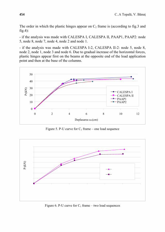
454 C..A Topală, V. Bănuţ
The order in which the plastic hinges appear on C2 frame is (according to fig.3 and fig.4):
- if the analysis was made with CALESPA I, CALESPA II, PAAP1, PAAP2: node 5, node 8, node 7, node 4, node 2 and node 1.
- if the analysis was made with CALESPA I-2, CALESPA II-2: node 5, node 8, node 2, node 1, node 3 and node 6. Due to gradual increase of the horizontal forces, plastic hinges appear first on the beams at the opposite end of the load application point and then at the base of the columns.
0
10
20
30
40
50
0 2 4 6 8 10 12
Deplasarea uA(cm)
P1(k
N)
CALESPA ICALESPA IIPAAP1PAAP2
Figure 5. P-U curve for C1 frame – one load sequence
P1(k
N)
Figure 6. P-U curve for C1 frame – two load sequences

“Computational Civil Engineering 2010”, International Symposium 455
P2(k
N)
Figure 7. P-U curve for C2 frame – one load sequence
0
20
40
60
80
100
120
140
160
0 5 10 15 20 25
Deplasarea uB(cm)
P2(k
N)
CALESPA I-2
CALESPA II-2
Figure 8. P-U curve for C2 frame – two load sequences
It was found that if the loads are applied in two sequences, plastic hinges appear on columns much earlier during the analysis.
The P-U curves determined for the two frames are presented in figures 5,6,7,8.
The one storey C1 frame reaches the maximum strength capacity by forming a total plastic failure mechanism.
According to CALESPA I application, the C2 frame reaches collapse due to the forming of a partial plastic failure mechanism. The plastic hinges appear first on the beams and then on the columns. Unlike the simple plastic method, other

456 C..A Topală, V. Bănuţ
applications (that are based on the second order analysis) determine first 3,4 plastic hinges and after that the stiffness matrix determinant becomes negative, meaning that the structure reaches collapse not by forming a plastic failure mechanism but by loosing its stability through continuous deformation. This observation is made also in the paper [3].
In the second order analysis, in all cases, both the ultimate force and its corresponding displacement are smaller than those obtained in the first order analysis. The failure force from the second order analysis decreases by about 11% of that in the first order analysis.
The influence of the physical nonlinearity in the analysis of structures is lower than the influence of the geometric nonlinearity. In general, the ultimate force value decreases (by 3-7%) and the corresponding displacements increase by considering the effects of material nonlinearity (stiffness decreasing).
Application of the loads in two sequences determines the failure forces to increase as well as their corresponding displacements.
The critical force multiplier, , was determined for a level of forces resulted from CALESPA I, CALESPA II, CALESPA I-2, CALESPA II-2 applications corresponding to the forming of the plastic hinges. The curves obtained by processing the STASEL results are similar to those from fig.9 and fig.10.
C1-CALESPA I
0
10
20
30
40
50
0 2 4 6 8 10 12
Deplasarea uA(cm)
P1
(kN
)/ λ
P-U λ-U
Figure 9. P-U and λ-U curves for C1 frame with the values obtained from CALESPA I
application
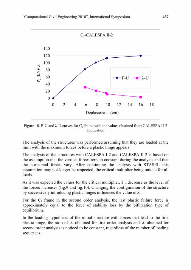
“Computational Civil Engineering 2010”, International Symposium 457
C2-CALESPA II-2
0
20
40
60
80
100
120
140
0 2 4 6 8 10 12 14 16 18
Deplasarea uB(cm)
P2
(kN
)/ λ
P-U λ-U
Figure 10. P-U and λ-U curves for C2 frame with the values obtained from CALESPA II-2
application
The analysis of the structures was performed assuming that they are loaded at the limit with the maximum forces before a plastic hinge appears.
The analysis of the structures with CALESPA I-2 and CALESPA II-2 is based on the assumption that the vertical forces remain constant during the analysis and that the horizontal forces vary. After continuing the analysis with STASEL this assumption may not longer be respected, the critical multiplier being unique for all loads.
As it was expected the values for the critical multiplier, , decrease as the level of the forces increases (fig.9 and fig.10). Changing the configuration of the structure by successively introducing plastic hinges influences the value of .
For the C1 frame in the second order analysis, the last plastic failure force is approximately equal to the force of stability loss by the bifurcation type of equilibrium.
In the loading hypothesis of the initial structure with forces that lead to the first plastic hinge, the ratio of obtained for first order analysis and obtained for second order analysis is noticed to be constant, regardless of the number of loading sequences.

458 C..A Topală, V. Bănuţ
2 2
20%
20%CALESPAII CALESPAI
CALESPAII CALESPAI
for C1 frame
2 2
36%
36%CALESPAII CALESPAI
CALESPAII CALESPAI
for C2 frame
4.1. Final conclusions
In order to analyse a structure in the nonlinear domain, it should obey the requirements for the material quality, the shape of the transversal section, the structural arrangement and the design.
By neglecting the second order effects, it leads to a higher plastic failure force and a higher critical force for stability loss.
The physical nonlinearity effects are lower than those of geometric nonlinearity.
The structure with one storey and one bay reaches collapse by forming a total failure mechanism and the structure with two stories and one bay reaches collapse by loss of stability by continuous deformation.
The order in which the plastic hinges appear and the way the structure collapses are directly influenced by the number of load sequences and the type of structural analysis.
Bibliography:
1. Bănuţ, V., Calculul neliniar al structurilor, Ed. Tehnică 1981. (in Romanian) 2. Bănuţ, V., Calculul de ordinul II şi de stabilitate al elementelor şi structurilor de rezistenţă, Ed.
Conspress, Bucuresti 2005. (in Romanian) 3. Bănuţ, V., Teodorescu, M. E., Despre limitele metodei plastice simple, Buletinul Ştiinţific nr. 2
UTCB, 2002. (in Romanian) 4. Chen, W. F., Seung-Eock Kim , LRFD Steel Design using Advanced Analysis, CRC Press, Florida
1997 5. Eurocode 3/1993, Design of Steel Structures 6. Cod de proiectare seismică P1001/2006 Prevederi de proiectare pentru clădiri. (in Romanian)

“Computational Civil Engineering 2010”, International Symposium Iasi, Romania, May 28, 2010
Steel structures with composite floors and energy dissipative columns
Vasile-Mircea Venghiac1, Ioan Petru Ciongradi1 and Mihai Budescu1
1Department of Structural Mechanics, “Gh. Asachi” Technical University, Iasi, 700050, Romania
Abstract
Energy dissipative systems are widely used for controlling vibrations and increasing the structural safety of constructions in seismic areas. Nowadays there are many types of dissipative systems consisting of different materials and methods. Generally, these systems transform the kinetic energy into other types of energy. In this paper the behavior of a steel structural system with composite floors and “dissipative” steel columns, subjected to a cyclic loading, is presented. The composite floor consists of embedding the steel beams in concrete, thus increasing the rigidity of the floor. In seismic zones these floors present a low energy dissipation capacity. In this case, “dissipative” steel columns are proposed for their structural rigidity contribution and also for the increased capacity of energy absorption. These columns absorb energy by deforming the steel up to yielding.
KEYWORDS: yielding steel damper; composite slab; SlimFloor; ADAS damper; cyclic loading; hysteretic damper; ANSYS.
1. INTRODUCTION
1.1. Composite flooring system
Composite floors consist of a steel decking and reinforced concrete poured in-situ. The decking acts as a permanent shuttering and also as the bottom reinforcement for the slab. After the hardening process ends, the decking works together with the concrete obtaining the composite behavior.
In this paper the SlimFloor composite flooring system is considered. SlimFloor is a generic term used to describe a form of construction where the supporting beams are contained within the depth of the concrete slab. This is achieved by supporting the slab off the bottom flanges of the beams. The beams have an asymmetric section with a narrower top flange than the bottom flange [4]. This type of flooring system is presented in figure 1.

460 Vasile-Mircea Venghiac, Ioan Petru Ciongradi, Mihai Budescu
Figure 1. The SlimFloor composite flooring system [4].
The SlimFloor system is particularly beneficial in providing the following: • Shallow floor depth. This may lead to savings in cladding cost, or help to
meet overall building height restrictions. This is the reason why they are also called shallow flooring systems.
• Ease of service integration. There is a potential to accommodate the services within the slab depth and between the ribs of the decking.
• Inherent fire resistance. A fire resistance of 60 minutes can be achieved without fire protection [4].
1.2. Yielding steel dampers
The dissipation of energy by plastic strain is obtained when the steel is deformed in plastic domain. Thus, energy is transformed into heat. The strained element can be subjected to bending, compression, tension, local buckling or by combining two or more actions. These systems can be uni-directional or multi-directional.
The advantage of yielding steel dampers is their stable behavior, remarkable reliability and also resistance to environmental conditions. Once implemented into a structure they increase the structural strength and rigidity and the energy absorption capacity.
There are many types of dampers that use the yielding capacity of steel to absorb energy. One of them is the V-shape plate damper or TADAS (Triangular plate Added Damping And Stiffness) [2]. Research carried out on these devices showed a good behavior to a big number of load cycles. The V-shape of the dissipative members, as shown in figure 2, ensures that the whole section is subjected to plastic strain [5, 6].

“Computational Civil Engineering 2010”, International Symposium 461
Figure 2. TADAS damper (Triangular plate Added Damping And Stiffness) [5,6].
An improved alternative of the TADAS damper is the X-shape plate damper or ADAS (Added Damping And Stiffness) introduced by Bechtel Power Corporation in 1985. This damper presents an increased rigidity, mainly because the dissipative plates are restrained at both ends. The ADAS damper is presented in figure 3.
Figure 3. ADAS damper (Added Damping And Stiffness) [5, 6].
A similar damper to TADAS and ADAS is the honeycomb damper [3] presented in figure 4.

462 Vasile-Mircea Venghiac, Ioan Petru Ciongradi, Mihai Budescu
Figure 4. Honeycomb damper [3].
Its dissipative members are made of steel plates with hexagonal openings. The rigidity of the honeycomb damper is larger than the ADAS and TADAS systems, and the shape can be optimized so that the whole dissipative member would strain up to yielding.
2. OBJECTIVES AND SCOPE OF WORK
The aim of this paper is to investigate the behavior of a composite flooring system with energy “dissipative” columns subjected to cyclic loading. In seismic zones the shallow composite flooring system presents some disadvantages. The most important is the low energy dissipation capacity. Embedding the beams in concrete eliminates the occurrence of plastic hinges which are the mechanisms of absorbing the seismic energy. Another objective of this paper is to introduce a damping device which will not block the window area as in the case of the TADAS, ADAS or the honeycomb damper as shown in figures 2, 3 and 4, respectively. In this case, energy “dissipative” columns are proposed.
Several such devices, similar to ADAS and to the honeycomb damper, were investigated. In the end the “dissipative” columns similar to the honeycomb device were the most effective.
The finite element program used for the analysis is ANSYS Workbench v12 [1].

“Computational Civil Engineering 2010”, International Symposium 463
3. MODELLING THE ENERGY DISSIPATIVE COLUMNS IN ANSYS
The damping system proposed consists of placing a secondary column next to the main columns and linking them with metallic plates as shown in figure 5. Another way of using this type of damping system is by making the two column ensemble separately and placing it strategically in the building. The shape of the dissipative members (metallic plates) follows a curve optimized so that the whole section strains up to yielding.
Figure 5. Energy "dissipative" columns.
The metallic plates were placed as pairs of two between the flanges of the columns and they have the following dimensions: 10 mm thickness, 40 mm width at the ends, 20 mm width at the middle and 200 mm in length. The columns are made of hot rolled HEA180 Euro-profiles. The height of the columns is 2.50 m, the distance

464 Vasile-Mircea Venghiac, Ioan Petru Ciongradi, Mihai Budescu
between their axes is 380 mm and the steel grade for all of the components is S235. The columns are restrained at the bottom.
Five models were considered, distributing the dissipative elements on the height of the columns as follows:
A. 1 pair of dissipative members on the middle height of the columns; B. 9 pairs at 100 mm apart on the middle height of the columns; C. 9 pairs distributed uniformly on the height of the columns; D. 9 pairs: 1 pair at the middle and 4 pairs at 100 mm apart at each end of the
columns; E. 23 pairs at 100 mm apart on the middle height of the columns.
4. RESULTS
The models were subjected to a load cycle under the form of imposed displacements on X direction. The value considered is 25 mm in both directions. After running the analysis in ANSYS [1], the whole section of the dissipative elements yielded as shown in figure 6.
Figure 6. Normal stress along X axis [1].
Several charts were plotted to compare the models and their behavior. The chart in figure 7 shows the difference of using one, several or the maximum possible number of dissipative elements. The best way of positioning the optimum number of dissipative elements is outlined in the chart presented in figure 8.

“Computational Civil Engineering 2010”, International Symposium 465
-150000
-100000
-50000
0
50000
100000
150000
-30 -20 -10 0 10 20 30
Displacement [mm]
For
ce [
N]
Model A
Model B
Model E
Figure 7. Comparison between models A, B and E.
-100000
-80000
-60000
-40000
-20000
0
20000
40000
60000
80000
100000
-30 -20 -10 0 10 20 30
Displacement [mm]
For
ce [
N]
Model D
Model B
Model C
Figure 8. Comparison between models B, C and D.

466 Vasile-Mircea Venghiac, Ioan Petru Ciongradi, Mihai Budescu
5. CONCLUSIONS
The analysis carried out on these models showed good results. The chart presented in figure 7 emphasizes the fact that using a large number of dissipative elements leads to small improvements of the damping capacity of the device. The most favorable way of increasing the energy dissipation capacity, according to the chart in figure 8, is to place the optimum number of dissipative members on the middle height of the columns because here occurs the maximum rotations. This also increases the rigidity of the damper.
The results obtained so far show the potential of this type of damping device. Further research will be carried out to improve its behavior by optimizing the shape of the dissipative elements, their distribution and position and also by changing the position and geometrical shape of the columns.
References
1. ANSYS (2009), User’s Manual Revision 11, ANSYS, Inc., Canonsburg, PA. 2. Kelly, J.M., Skinner, M.S., The Design of Steel Energy-Absorbing Restrainers and their Incorporation into Nuclear Power Plants for Enhanced Safety, vol. 4, Review of current Uses of Energy-Absorbing Devices, UCB/EERC – 79/10. 3. Piccione, Denise, Principi constitutivi e tecnologia dei dispositivi per l’isolamento sismico delle strutture, Tesi di laurea, Politecnico di Torino, 1995. 4. Rackham, J.W., Couchman, G.H., Hicks, S.J., Composite Slabs and Beams using Steel Decking: Best Practice for Design and Construction, Revised Edition, The Steel Construction Institute and The Metal Cladding & Roofing Manufacturers Association, 2009. 5. Sadek, F., Mohraz, B., Taylor, A.W., Passive Energy Dissipation Devices for Seismic Applications, Building and Fire Research Laboratory, Gaithersburg, Maryland, National Institute of Standards and Technology, NISTIR 5923. 6. Tyler, R.G., Damping in building structures by means of PTTF sliding joints, Bulletin of New
Zeeland Society of Earthquake Engineering, vol. 10, 1977.
“Computational Civil Engineering 2010”, International Symposium Iasi, Romania, May 28, 2010
Static Modulus of Elasticity of High Strength Concrete
Dumitru Moldovan1, Cornelia Măgureanu2 1Reinforced and Prestressed Concrete Department, Technical University of Cluj-Napoca, Cluj-
Napoca, 400114, Romania 2Reinforced and Prestressed Concrete Department, Technical University of Cluj-Napoca, Cluj-
Napoca, 400114, Romania
Summary
High Strength Concrete has been in recent years the object of intensive study due to its numerous advantages over Normal Strength Concrete. Contrary to other Special Concretes such as Ultra High Performance Concrete or Reactive Powder Concrete, High Strength Concrete is becoming increasingly more available to contractors and thus more common to jobs all over the world.
The need to provide clear guidance to contractors for full potential achievement of this new-standard-becoming-material is therefore, more than ever, mandatory.
This study will provide an extended coverage on the relationships for the Static Modulus of Elasticity, as defined by current code provisions or previous studies by other authors, in view of a particular research for C60 and C80 grade concretes.
KEYWORDS: modulus of elasticity, high strength concrete, research
1. INTRODUCTION
Load behaviour of a concrete member, from a microscopic point of view, is defined by gradual crack development that will lead to a spatial pattern distributed inside the whole volume of that member. As the load reaches the strength of the material, this pattern will evolve as a bi-phased process, first of which being the stop of any crack increase (in length and diameter) and the second being the further increase of cracks (also in length and diameter) in a rather small part of the member’s volume. This second phase, also known as crack localization, will cause the members to fail starting from the area where the fore mentioned phenomenon appeared. Therefore, failure is, in the case of brittle materials such as concrete, a gradual process governed by the cracking pattern established inside the volume of the member under loading.
If one were to control the cracking process, that should be done by (1) maintaining the load up to a level that does not lead to crack localization and (2) by cyclically loading and unloading of the member to allow for all possible cracks, for that level

468 D. Moldovan, C. Măgurenu
of loading, to appear. In this manner, the so called crack softening effect will take place and the brittle material acts as if being an elastic one (i.e. the ascending branch and the descending one, for loading, in stress-strain coordinates, will cease to enclose an area), therefore no hysteresis will occur, [1] (Cadar et al., 2004, Beton Armat).
without hysteresis with hysteresis with hysteresis
Non-linear elastic Elastic-plastic Elastic (non-linear)-viscous
Figure 1. Elastic, plastic and viscous strains, [1]
In the case of High Strength Concrete it is well known the proportionality of the strains with the stresses (or vice versa) for an applied load with is about 90% of the ultimate stress (strength of the material) [2] (MĂGUREANU, 2003, Betoane de Înaltă rezistență și Rezistență). Therefore, the unloading of a given specimen, which is under a maximum stress of about half of the earlier specified limit, will show the same behaviour as the loading itself. That being the case, it is right to asses that for High Strength Concrete the Modulus of Elasticity (MOE) is the same regardless of the combination of stress and strain that define a given modulus, as illustrated in fig. 2.
2. PROPOSED FORMULAS FOR MOE
In the following paragraphs, the author will present a number of proposed relationships for MOE, for compressive strengths ranging from 50 MPa to 110 MPa. The list is not limiting the choices one may have in assessing MOE for a given mix, but will provide, in this author’s opinion, valuable sources for comparison, in view of previously published results. Those results are then applied to a research the author took part in actively, by using the mean value for the compressive strength of the concrete as specified by the code provisions, [3] (SR EN 1992-1-1:2004, 2004, Eurocod 2: Proiectarea structurilor de beton…).

“Computational Civil Engineering 2010”, International Symposium 469
The values provided are expressed in GPa, which will be omitted for clearance. Further notes are available in each case for the same purpose (i.e. wc – the density of concrete).
Incr
ease
in s
tres
s
Increase in strain
Figure 2. Various types of the Modulus of Elasticity, [3]
▪ L. J. PARROTT (1979), [4] (Simplified Methods of Predicting...)
0.25 , for 40 90c o cm cmE C f MPa f MPa (1.a), with
15 , for small and medium aggregates' MOE
25 , for medium and high aggregates' MOE
0.4 ,as a function of aggregates' MOEo
a
GPa
C GPa
E
(1.b)
The formula above is modified by multiplying with a factor of 1.25 to account for the difference between the compressive strength of concrete on cubic test specimens to cylindrical ones.
▪ S. P. SHAH and S. H. AHMAD (1985), [5] (Structural Properties...)
2 0.3253.385 10 , for 84c c cm cmE w f f MPa (2)
▪ Fuminori TOMOSAWA and Takafumi NOGUCHI (1990), [6] (Relationship between Compressive Strength...)
12
3
1 233.852400 60
c cmc
w fE k k
(3.a), with

470 D. Moldovan, C. Măgurenu
1
1, 20 crushed limestone, calcinated bauxite
0,95 crushed aggregates , , , ,
1,00 coarse aggregates
k quartzitic andesite basalt clayslate cobbel stone
other than the above
(3.b), correction factor due to coarse aggregates
2
0,95 silica fume, ground granulated blast-furnace slag, fly ash fume
1,10 fly ash
1,00
k
other than the above
(3.c), correction factor due to the type of addition ▪ NS 3473 (1992), [7] (Concrete Structures...)
0.39.5 , for 25 85c cm cmE f MPa f M Pa
cmf
(4)
▪ RADAIN, SAMMAN and WAFA (1993), [8] (Mechanical Properties of High-Strength Concrete)
0.514.495 2.176cE (5)
▪ Said IRAVANI (1996), [9] (Mechanical Properties of High-Performance Concrete)
4.7 , for 55 125c a cm cmE C f MPa f MPa (6.a), with
0,71 sandstone gravel
0,76 siliceous gravel
0,92 limestone or dolomite
0,97 quartzites
0,82 granite
0,97 trap rock
0,90 diabase
0,61 sandstone
aC
(6.b), correction factor due to coarse aggregates
▪ AITCIN et al. (2002), [10] (Determination of elastic properties of...)
0.55.05cE cmf (7)
▪ H. Abdul RAZAK and H.S. WONG (2004) – test based formulas, [11] (Re-evaluation of strength...)
4.026 1.037c cmE f (8.a)
4.138cE f cm (8.b)

“Computational Civil Engineering 2010”, International Symposium 471
0.6151.98 7.708c cmE f (8.c)
0.4844.452c cmE f (8.d)
0.818c cmE f (8.e)
▪ Peter B. KEATING et al. (2004), [12] (Mechanical Properties of High-Strength Concrete...)
0.55.23 , for 40 90c cm cmE f MPa f M Pa (9)
▪ ACI 363R-1992 (2005), [13] (State-of-the-Art Report...)
3.32 6.9c cmE f (10)
▪ ACI 318:2008 (2008), [14] (Building Code Requirements...)
1.50.043c cE w cmf (11.a), with various densities
4.73c cE f m (11.b), for normal density concrete
▪ fib (2009), [15] (fib Bulletin no. 42, Constitutive modelling...)
1 1
3
, ,
8
10 10ck cm
ci c o E c o E
f MPa fE E E
3
MPa MPa
P
(12.a), with
, 20,5c o aE G (12.b)
1.20 basalt, dense limestone aggregates
1.00 quartzitic aggregates
0.90 limestone aggregate
0.70 sandstone aggregates
sE
(12.c), correction factor
due to the type of coarse aggregates
The above presented have been used to graph figure 3. Several conclusions may be therefore extrapolated, such as:
1. for the lower limit of MOE as obtained for our studied mix, the mean value is that proposed by Equation (2) in [5] (SHAH, AHMAD, 1985, Structural Properties...)
2. for the upper limit, the mean value is that given by Equation (12.a) in [15] (fib, 2009, Bulletin no. 42, Constitutive modelling...)
3. the mean fit for the studied domain is given by the same equation as above 4. the large spread in data may be attributed to the variations in the chemical
and physical properties of the constituents used by the different authors for their studies. This is a common problem that mainly affects High Strength

472 D. Moldovan, C. Măgurenu
Concrete as opposed to Normal High Strength Concrete, which is less averted by, in general speaking, the technology used to produce any given mix.
5. It is obvious then that the simplified formula for MOE as depending only on the compressive strength of concrete may, in most cases, lead to gross approximations.
In order to compensate such errors, some authors proposed formulas that take into consideration the influence of the density of concrete, either directly or by dividing it by a referenced value, or the influence of the type of aggregates, or the influence of the type of the addition.
MO
E (
GP
a)
Compressive strength (MPa)
Figure 3. Comparison of the different formulas for MOE
The values graphed in Figure 3 are based on the assumption that: in Equation 1, 25oC GPa for medium and high aggregates’ MOE
in Equation 3, 1 0,95k correction factor due to coarse aggregates (quartzitic)
and correction factor due to type of addition (silica fume) 2 0,95k
in Equation 6, 0.82aC (granite aggregates)
in Equation 12, 1.00E (quartzitic aggregates)
Nonetheless even such formulas fail to take into consideration the variations in water/cement ratio (W/C) or water/binder ratio (W/B), shape, dimension and position during casting of the member, curing conditions or the age at testing, each with a known influence over the behaviour of concrete in service, [16]

“Computational Civil Engineering 2010”, International Symposium 473
(MOKHTARZADEH and FRENCH, 2000, Mechanical Properties of High-Strength Concrete with…) or [2] (MĂGUREANU, 2003, Betoane de Înaltă rezistență și Rezistență).
MO
E (
MP
a)
Compressive strength (MPa)
Figure 4. Comparison of the different values for MOE in use by given national codes
For this reason we present proposed relationships by different authors such as [17] (BERKE et al., 1992, Plastic, Mechanical, Corrosion…) or [18] (MOSTOFINEJAD and NOZHATI, 2005, Prediction of the modulus...). To allow a better clearance, the following short forms will refer to: water/cement ratio (W/C), silica fume/cement ratio (S/C), age (t), MOE and percentage (in volume) for aggregates ( ), or MOE and percentage (in volume) for cement paste
(
,a aE g
,g gE g ).
▪ N. S. BERKE et al (1992), [17] (Plastic, Mechanical, Corrosion…)
3 332.297 10 71.963 10 3.121 ln 12.391 c
W St
C CE (13)
▪ MOSTOFINEJAD and NOZHATI (2005), [18] (Prediction of the modulus...), for composite materials
, g m mc VE E gE aa (14.a), Voigt model
,
g
1 m
c R am
g
EE E a (14.b), Reuss model

474 D. Moldovan, C. Măgurenu
,,
1
1 1
2
1
c cc V REE E
(14.c), Hirsh-Dougill model
, , 1
2 c Rcc VE E E (14.d), Popovics model
1
1 11 a a
m ac m a
g gE E
E E g
(14.e), Counto model
( ) ( )
( ) (
)m a m a a
cm a m a a
E E E E gE
E E E E g mE
(14.f), Hashin model
m ag gc m aE E E (14.g) Bache and Nepper-Cheistensen model
▪ MOSTOFINEJAD and NOZHATI (2005), [18] (Prediction of the modulus...), for various types of aggregates
0.31610.25 cmc fE (15.a), limestone
0.3528 cmcE f (15.b), andesite
0.31210.75 cmc fE (15.c), quartzite
▪ MOSTOFINEJAD and NOZHATI (2005), [18] (Prediction of the modulus...), for a given W/C, S/C and t
0.270.0514
0.18
26.84 1c
t S CE
W C
(16.a), limestone
0.290.0539
0.19
24.36 1c
t S CE
W C
(16.b), andesite
▪ MOSTOFINEJAD and NOZHATI (2005), [18] (Prediction of the modulus...), for all of the above
0.280.3 0.053
0.18
8 1ac
E t S C
CE
W
(17.a), given aE
0.280.053
0.18
26.8 1c
t S CE
W C
(17.b), unknown aE

“Computational Civil Engineering 2010”, International Symposium 475
3. RESEARCH PROGRAM
3.1. Member casting
The results presented herein are possible due to the following research programs: [19] Grant A (1036/2004, Betoane de Înaltă Rezistență și Performanță...) and [20] TD (280/2007, Ductilitatea Betoanelor de Înaltă Rezistență și Performanță). Both studies aided at describing the behaviour of High Strength Concrete under various conditions by testing to rupture a number of 14 beams for two concrete grades, C60 (8 beams) and C80 (6 beams). Our opinion presented here is based on the accompanying test specimens.
The mix proportions have been established based on the previous experience of the research team at the Reinforced and Prestressed Concrete Department from the Faculty of Civil Engineering in Cluj-Napoca. The matrix consists basically of type CEM I Portland Cement provided by LAFARGE, silica fume provided by SIKA, and local crushed aggregates of 0-4 [mm], 4-8 [mm] and 8-16 [mm] provided by MORLACA quarry. W/C ratio is 0.266. A policarboxilate plasticizer under the commercial name of RAVENIT, at a dosage of 0.88 [%], has been added to improve mix properties. Unless otherwise specified, the units are in [kg/mc] and are omitted for clearance.
Table 1. Mix proportions C60(C80) grade Type C60 grade C80 grade
Cement CEM I 52.5 R
480 520
Coarse aggregates 8-16 [mm] 706 706 Aggregates 4-8 [mm] 530 530 Sand 0-4 [mm] 530 530 Silica fume SIKA 48 52 Super plasticizer RAVENIT 13.5 [l/mc] 13.5 [l/mc] Water plain 152 [l/mc] 152 [l/mc] Water/Cement (W/C) 0,32 0,29 Water/Binder (W/B) 0,29 0,27
Each casted beam has been accompanied by a number of at least three cubes of 150 mm and at least three prisms of 100 by 100 by 300 mm, cured under the same conditions as the beams. Two curing conditions were investigated: under water (at
) and standard ( for 20 2o oC C C20 2o oC 60% 5%RH ). Compressive strength for concrete has been studied at 28 days and the age of testing for the beams (approximately 90 days). The MOE has been established as prescribed at 28 days.

476 D. Moldovan, C. Măgurenu
The testing machine used in uniaxial compression is an Advantest 9 type, first class precision equipment with a maximum frame load of 3000 kN. The load has been set to a constant ratio of 1N/mm2.
3.2. Data collected
As anticipated, the data of interest for the current paper is the one about MOE. Testing procedure in use as mandatory by national code provisions has been use to determine MOE on 100 by 100 by 300 mm test prism under cyclic constant load control. Each result presented herein is the medium value of three consecutive tests.
Table 2. Experimental MOE
Beam no Grade Value Units 80
60
C
C
MOE
MOE
I 1 C60 45.48 I 2 C60 45.64 I 3 C60 45.24 I 4 C60 46.34
[GPa] -
BH 1 C80 45.40 BH 2 C80 47.20 BH 3 C80 47.08
[GPa] 1.019
The proposed formulas as presented in Chapter 2 will be checked for consistency against the above data. The purpose of this endeavour is to determine which model is a best fit and to present a personal point of view of the author on the subject at hand.
3.3. Comparison with proposed formulas
From Table 2 the mean values for MOE have been calculated as 45.68 [GPa] for C60 and 46.56 [GPa] for C80. Those values (labelled “EXP”) are represented along with all the results for the proposed formulas, with respect to the above two concrete grades, in Figure 5.
It can be seen that the experimental values are above all of the calculated values. Also, there is little difference among the experimental results (less than 3%) which does not follow the trend set by the difference in compressive strength (about 30%). In these authors’ opinion, the results obtained clearly show that the ratio of MOE vs. compressive strength is decremental as the concrete grade increases up to a point. Beyond this limit the results show a flat variation in spite of further increase in the compressive strength.

“Computational Civil Engineering 2010”, International Symposium 477
3.4. Comparison among proposed formulas
For the reasons presented above it is for the better to analyse the proposed formulas against each other by taking into consideration the model presented by the national code provisions [3] (SR EN 1992-1-1:2004, 2004, Eurocod 2: Proiectarea structurilor de beton…), defined by:
0.3
2210
cmcm
fE
MPa
(18)
For the studied concrete grades MOE is 39 [GPa] and 43 [GPa] respectively. The data analysis is presented in Table 3 (units in GPa omitted for clearance).
MO
E (
GP
a)
Compressive strength (MPa)
Figure 5. Comparison of proposed formulas with experimental results
As presented, the best fit for the experimental data is that given by KEATING et al. (2004), [12] (Mechanical Properties of High-Strength Concrete...) for both concrete grades under study, with an interval (limited by the maximum and the minimum calculated) of about 1/3 of the calculated MOE.

478 D. Moldovan, C. Măgurenu
Table 3. Data analysis C60 C80 Experimental results 45.68 46.56 Code provisions 39 43 Maximum (proposed formulas) 40.51 (9) 46.78 (9) Minimum (proposed formulas) 28.48 (8.e) 33.96 (5) Interval (maximum-minimum) 12.03 12.82 Mean (proposed formulas) 34.50 40.37 Subtraction (mean from experimental) 11.18 6.19 Subtraction (maximum from experimental) 5.16 -0.22 Subtraction (minimum from experimental) 17.20 12.60
Confidence interval (mean 5% ) 32.77-36.22
38.35-42.39
4. CONCLUSIONS
In these authors’ opinion the interval defined by the studied formulas (about 1/3) points to the conclusion that High Strength Concrete is very sensitive to any variation in the constituents’ properties, either mechanical, physical or chemical. Still, this does not account for the huge spread in data, making it mandatory to propose better models for MOE evaluation.
The best fit for the presented experimental data is that given by KEATING et al. (2004), [12] (Mechanical Properties of High-Strength Concrete...) for both concrete grades under study. The obtained result is higher with about 12% in the case of C60 concrete grade and is about the same for C80.
As compared with the national code provisions, the obtained results are also higher, with about 17% for C60 and about 8% for C80. Due to the lack of data to support an explanation on this behaviour it is these authors’ opinion that further research is mandatory.
Acknowledgements
The author wishes to thank for their support to all of his colleagues and especially prof. Cornelia Măgureanu for her continuous and valuable advice.
The research program has been possible with the financial support of CNCSIS (Consiliul National al Cercetarii Stiintifice din Invatamantul Superior).
References
1. Cadar, I., Clipii, T., Tudor, A., Beton Armat, Ediția a 2-a, rev., Ed. Orizonturi Universitare, Timișoara, 2004, pag. [33-35]

“Computational Civil Engineering 2010”, International Symposium 479
2. Cornelia MĂGUREANU, Betoane de Înaltă rezistență și Rezistență, Ed. UT Press, Cluj-Napoca, 2003, pag. [100-112]
3. SR EN 1992-1-1:2004, Eurocod 2: Proiectarea structurilor de beton. Partea 1-1: Reguli generale şi reguli pentru clădiri, Asociaţia de Standardizare din România (ASRO), Ediţia 1, 2004, pag. [24-31]
4. L. J. PARROTT, Simplified Methods of Predicting the Deformation of Structural Concrete, Development Report No. 3, Cement and Concrete Association, October 1979, pag. [1-11]
5. S. H. AHMAD, S. P. SHAH, Structural Properties of High-Strength Concrete and its Implications for Precast Prestressed Concrete, PCI Journal, vol. 30, no. 6, 1985, pag. [92-119]
6. Fuminori TOMOSAWA, Takafumi NOGUCHI, Relationship Between Compressive Strength And Modulus Of Elasticity Of High-Strength Concrete, New RC Project, 1990, pag. [1-8]
7. Norwegian Standard NS 3473, Concrete Structures – Design and detailing rules, The Norwegian Council for Building Standardisation, N.B.R., Oslo, Norway, 1995
8. T.A. RADAIN, T.A. SAMMAN, F.F. WAFA, Mechanical Properties of High-Strength Concrete, Proceedings of the Third International Symposium on Utilization of High-Strength Concrete, V. 2, Lillehammer, Norway, 1993, pag. [1209-1216]
9. Said IRAVANI, Mechanical Properties of High-Performance Concrete, ACI Materials Journal, vol. 93, no. 5, September-October 1996, pag. [1-11]
10. Habib A. MESBAH, Mohamed LACHEMI, Pierre-Claude AÏTCIN, Determination of elastic properties of HPC at early ages, ACI Materials Journal, vol. 99, no. 1, January-February 2002, pag. [37-41], http://www.sciencedirect.com, accessed on 5 mar. 2009
11. H. Abdul RAZAK, H.S. WONG, Re-evaluation of strength and stiffness relationships for High-Strength Concrete, Asian Journal Of Civil Engineering (Building And Housing), Vol. 5, No. 1-2, 2004, pag. [85-99], http://www.bhrc.ac.ir/Publication/AJCE/PDF/Vol5-No1-2/Abdulrazagh-6.pdf, accessed on 4 mar. 2009
12. Mary Beth D. HUESTE, Praveen CHOMPREDA, David TREJO, Daren B. H. CLINE, Peter B. KEATING, Mechanical Properties of High-Strength Concrete for Prestressed Members, ACI Structural Journal, vol. 101, no. 4, July-August 2004, pag. [457-465], http://www.sciencedirect.com, accessed on 5 mar. 2009
13. ACI Committee 363, State-of-the-Art Report on High-Strength Concrete (ACI 363R-92), ACI Manual of Concrete Practice, Part 5, 2005, pag. [363R1-363R55]
14. ACI Committee 318, Building Code Requirements for Structural Concrete (ACI 318-08) and Commentary, Chapter 8 – Analysis and Design – General Considerations, 8.5. Modulus of Elasticity, First Printing, January 2008, pag. [103-113]
15. fédération internationale du béton (fib), Bulletin no. 42, Constitutive modelling of high-strength/high-performance concrete, February 2009, pag. [23-29]
16. Alireza MOKHTARZADEH, Catherine FRENCH, Mechanical Properties of High-Strength Concrete with Consideration for Precast Applications, ACI Materials Journal, vol. 97, no. 2, March-April 2000, pag.[136-148]
17. N. S. BERKE, M. P. DALLAIRE, M. C. HICKS, Plastic, Mechanical, Corrosion and Chemical Resistance Properties of Silica Fume (microsilica) Concretes, ACI Special Publication, vol. 132, May 1 1992, pag. [1125-1150]
18. D. MOSTOFINEJAD, M. NOZHATI, Prediction of the modulus of elasticity for HSC, Iranian Journal of Science & Technology, vol. 29, no. B3, June 2005, pag. [311-321], http://www.sid.ir/en/VEWSSID/J_pdf/8542005B306.pdf , accessed on 22 oct. 2009
19. Grant A, 1036/2004, Betoane de Înaltă Rezistență și Performanță realizate cu fibre de oțel, de carbon și pulbere de cauciuc. Comportarea în zone seismice, medii agresive, solicitri dinamice și de uzură. Ecologia Mediului (director prof. dr. ing. Cornelia MĂGUREANU) TD 280/2007, Ductilitatea Betoanelor de Înaltă Rezistență și Performanță (director asist. drd. ing. Hegheș BOGDAN)

“Computational Civil Engineering 2010”, International Symposium Iasi, Romania, May 28, 2010
Application of fluid viscous dampers in the seismic control of steel frame structures
Horaţiu-Alin Mociran1, Eugen Panţel1 and Alexandra-Denisa Danciu1 1Faculty of Civil Engineering, Technical University, Cluj-Napoca, 400027, Romania
Summary
The purpose of this paper is to compare the seismic responses of a five storey, three bay steel frame structure with and without linear fluid viscous dampers and subjected to the same level of Kobe earthquake.
The steel frame was equipped with viscous dampers that provide two total damping ratios in the fundamental mode: 25% and 35%.
The seismic response parameters taken into account were: base shears, story drifts and story shears forces versus drifts loops.
The results of the performed nonlinear time history analysis indicate that dampers significantly reduce the seismic response and improve the behavior of the structure.
KEYWORDS: fluid viscous dampers, steel frame structures, time history analysis, earthquake, damping ratio, seismic response.
1. INTRODUCTION
The use of fluid viscous dampers represents a feasible alternative to enhance the seismic response of the structures and reduce the damages caused by earthquakes.
Fluid viscous dampers operate on the principle of fluid flow through orifices. A stainless steel piston travels through chambers that are filled with silicone oil. The pressure difference between the two chambers cause silicon oil to flow through an orifice in the piston head and seismic energy is transformed into heat, which dissipates into the atmosphere [1].
Fluid viscous dampers consume a significant portion of earthquake induced energy in the structure and minimize the hysteretic energy dissipated by the structural members.

“Computational Civil Engineering 2010”, International Symposium 481
2. THE STRUCTURE, FLUID VISCOUS DAMPERS AND THE SEISMIC MOTION
2.1. The structure
In order to study the efficiency of the dampers in reducing the seismic response, a five storey, three span steel frame structure was analyzed in two cases: unequipped and equipped (Figure 1). The unequipped structure was design to remain in the elastic range under the Kobe earthquake. The static design was made according to Eurocode 3 [2] and the seismic design was made according Eurocode 8 [3]. The dead load was considered 4 kN/m2 and the live load 2kN/m2. The distance between frames was assumed 6m.
HE
B36
0H
EB
360
HE
B30
0H
EB
300
HE
B26
0
HE
B36
0H
EB
360
HE
B30
0H
EB
300
HE
B26
0
HE
B36
0H
EB
360
HE
B30
0H
EB
300
HE
B26
0
HE
B36
0H
EB
360
HE
B30
0H
EB
300
HE
B26
0
IPE550 IPE550 IPE550
IPE550IPE550IPE550
IPE450
IPE450 IPE450
IPE450 IPE450
IPE450
IPE360 IPE360 IPE360
3.0
3.0
3.0
3.0
3.0
6.0 6.0 6.0
Figure 1. Transverse cross section of viscous damped frame

482 H. A. Mociran, E. Panţel, A. D. Danciu
2.2. Fluid viscous dampers
The structure was equipped with fluid viscous dampers of FIP INDUSTRIALE type placed within a diagonal configuration in all stories of the central bay of frame. The inherent damping ratio in the fundamental mode was assumed 5% and the total damping ratio of the equipped structure was designed as 25% and 35%.
Figure 2. FIP INDUSTRIALE viscous damper
2.3. The seismic motion
The seismic performances of the structures (unequipped and equipped) were investigated by time history analyses using Kobe earthquake.
Figure 3. Accelerogram of Kobe earthquake
3. TIME HISTORY ANALYSIS RESULTS
The seismic performances of structures were evaluated in terms of peak base shears, peak story drifts/ height and story shear forces versus story drifts loops.

“Computational Civil Engineering 2010”, International Symposium 483
3.1. Peak base shear
In Figures 4, 5 and 6 are presented the base shear time history for the three analyzed cases.
Figure 4. Base shear time history of the unequipped structure 0.05ef
Figure 5. Base shear time history of the equipped structure 0.25ef

484 H. A. Mociran, E. Panţel, A. D. Danciu
Figure 6. Base shear time history of the equipped structure 0.35ef
It can be seen that the maximum base shear was reduced by 21.77% for the equipped structure with damping ratio 0.25ef and by 27.07% for the equipped
structure with 0.35ef , compared to the unequipped structure.
3.2. Peak story drift/ Height [%]
The 4th story drift/height [%] time history for the equipped and unequipped structure are shown for example in Figures 7, 8 and 9.
Figure 7. 4th story drift time history of unequipped structure 0.05ef

“Computational Civil Engineering 2010”, International Symposium 485
Figure 8. 4th story drift time history of equipped structure 0.25ef
Figure 9. 4th story drift time history of equipped structure 0.35ef
Table 1. Peak story drift/ height [%] results 0.05 0.25 0.35 Floor
max / %rd h max / %rd h Reduction ratio [%]
max / %rd h Reduction ratio [%]
5 0.535 0.216 59.626 0.158 70.467 4 0.638 0.304 52.351 0.242 62.069 3 0.670 0.364 45.672 0.304 54.627 2 0.500 0.315 37.000 0.278 44.400 1 0.380 0.282 25.789 0.259 31.842

486 H. A. Mociran, E. Panţel, A. D. Danciu
The peak story drifts/ height [%] for the considered structures are given in Table 1. The reductions of the maximum story drifts at all floors are higher for the viscous damped structure with 0.35ef [4].
3.3. Story shear force - drift loop
A comparison of normalized story shear force versus story drift loops for the 4th story of the unequipped and equipped structure is presented for instance in Figures 10 – 12.
Figure 10. 4th story shear force - drift loop of the unequipped structure 0.05ef
Figure 11. 4th story shear force - drift loop of the equipped structure 0.25ef

“Computational Civil Engineering 2010”, International Symposium 487
Figure 12. 4th story shear force - drift loop of the equipped structure 0.35ef
One of the main advantages of fluid viscous dampers is that they produce simultaneous reductions of columns forces and story drifts of the equipped structure.
4. CONCLUSIONS
The paper compares the seismic responses of a five storey, three bay steel frame structure without and with linear fluid viscous dampers placed within diagonal configuration and subjected to Kobe earthquake. The obtained numerical results indicate that dampers reduced the peak drifts by 25.79 % to 59.63 % for a total damping ratio in the fundamental mode 0.25ef and by 31.84 % to 70.47% for
0.35ef
0.25ef
. Fluid viscous dampers reduce also the peak base shear by 21.77% for
and by 27.075 for 0.35ef .
The observed simultaneously reduction of story drifts and shear forces represents one of the main advantages of fluid viscous dampers compared to other passive energy dissipation devices.
References
1. Taylor, D., Duflot, P., Fluid viscous dampers used for seismic energy dissipation in structures, 2004, http://www.taylordevices.eu.
2. Eurocode 3, Design of steel structures, Brussels, 2003. 3. Eurocode 8, Design of structures for earthquake resistance, Brussels, 2003. 4. Mociran, H. A., Stan A. D., The influence of damping ratios on eathquake response of steel frame
structures, Computational Civil Engineering, Iaşi, 2008.
“Computational Civil Engineering 2010”, International Symposium Iasi, Romania, May 28, 2010
Altiscad Intellishape® Software for seismic design of reinforced concrete structures
Gheorghe Ionică Technical Manager, Altiscad Software Ltd., Bucharest, Romania
Summary
Software used by engineers in current practice of reinforced concrete structures’ analysis and design requires some very specific data in both main stages: analysis and design. Introduced data in analysis should be carefully reproduced by right design decisions; the quantity of reinforcement and its distribution should be a guarantee that the structure will behave as engineer presumed. The ductility behavior of the entire structure and each element contribution should be reflected in reinforcement amount and pattern.
The software presented is a specialized tool in design and checking of reinforced concrete structures placed in seismic areas. Used together with every day tools of design like 3D finite element software for seismic or spectral analysis, Altiscad Intellishape fills the gap between analysis and the stage of detailing and design.
KEYWORDS: demand ductility, plastic analysis, reinforced concrete, crack, reduced moment of inertia, reinforcement ratio.
1. INTRODUCTION
The most important challenges in seismic design of reinforced structures may be summarized as follows:
• Actual modern architectural shapes of structures cannot fulfill the structural regularity requirements of design codes. Instead of structural regularity and symmetry, engineers must lead the design concepts in order to achieve a structure’s dynamical regular behavior; a structure with a smooth dynamical behavior will act in case of dynamic forces (like seismic ground motion, waves, wind) as a structure with geometric regularities and symmetry;
• The development of plastic hinges, their appearance order and magnitude, must be carefully anticipated;
• The overall behavior of the structure has to be accordingly with expected performance criteria’s.

“Computational Civil Engineering 2010”, International Symposium 489
In practice, the implementation of design strategies that are used to fulfill mentioned requirements is done in a few steps.
2. STRUCTURE MODELING
In the first step, a needed performance criterion is chosen: a behavior factor (demand ductility).
Figure 1. Behavior factor definition in Autodesk Robot Structural Analysis
A value higher than one of behavior factor means that the structure has the capacity to dissipate induced seismic energy. A behavior factor equal to one signifies that the structure will always remain in elastic range, and no plastic hinges will be developed.
On the other hand, the value introduced by the user is just a demand, and not a guaranty that the structure will really behave like expected. Later, using results in elements, designer should find the reinforcement ratio and pattern which will determinate a structure response in concordance with demanded behavior.
Elements’ properties should be modified in order to simulate the presence of cracks. This happens because we assumed that structure will dissipate energy in form of plastic hinges, together with demand ductility (behavior factor).
Usually, altered sections (cracked or reduced sections) are defined by introducing a reducing factor for section’s moment of inertia or by decreasing the elasticity modulus of materials.

490 G Ionică
Figure 2. Reduction of moment of inertia in Autodesk Robot Structural Analysis for beams
and columns
The reduction of moment of inertia should be performed for plates and walls, too.
Figure 3. Reduction of moment of inertia in Autodesk Robot Structural Analysis for plates or walls
From structural modeling point of view, adjoined elements, forming zones with elevated rigidity should be considered like one element, so called core elements.

“Computational Civil Engineering 2010”, International Symposium 491
Figure 4. Core walls definition in Autodesk Robot Structural Analysis
3. RESULTS ANALYSIS
Regarding the capacity of vertical elements, at least three types of check must be done: overall capacity of the building (overturning moment, shear capacity etc.), capacity of each element, and the capacity of core elements.
In order to complete overall capacity check we can use the sum of reactions with opposite sign.
Singular elements, columns or walls, must be checked under axial force and biaxial bending moment. In case of walls, reduced forces must be used for the bottom part.
Core walls may be checked as one element but, depending of its configuration, we can also analyze the compounded elements, too.
All checking we mentioned can be fulfilled automatically using Autodesk Robot Structural, Autodesk Revit Structure and Altiscad Intellishape.

492 G Ionică
Figure 5. The 3D model of a structure in Autodesk Revit Structure with real reinforcement and the capacity diagrams of the entire first level from Altiscad Intellishape
Having analyzed the entire level of a building (Figure 5) we can automatically extract each element and analyze it separately.
Figure 6. Capacity diagrams of a reinforced concrete column
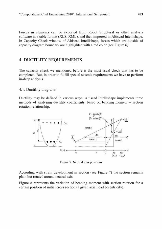
“Computational Civil Engineering 2010”, International Symposium 493
Forces in elements can be exported from Robot Structural or other analysis software in a table format (XLS, XML), and then imported in Altiscad Intellishape. In Capacity Check window of Altiscad Intellishape, forces which are outside of capacity diagram boundary are highlighted with a red color (see Figure 6).
4. DUCTILITY REQUIREMENTS
The capacity check we mentioned before is the most usual check that has to be completed. But, in order to fulfill special seismic requirements we have to perform in-deep analysis.
4.1. Ductility diagrams
Ductility may be defined in various ways. Altiscad Intellishape implements three methods of analysing ductility coefficients, based on bending moment – section rotation relationship.
Figure 7. Neutral axis positions
According with strain development in section (see Figure 7) the section remains plain but rotated around neutral axis.
Figure 8 represents the variation of bending moment with section rotation for a certain position of initial cross section (a given axial load eccentricity).

494 G Ionică
Figure 8. Diagram of Bending moment vs Section rotation
Based on Moment-Section rotation relationship, the q ratio can be defined as shown in Figure 9.
Figure 9. Ductility coefficients definition

“Computational Civil Engineering 2010”, International Symposium 495
It is obvious that the capacity diagram is influenced by the quantity of reinforcement. Replacing the real reinforcement ratio with other reinforcement ratio, but keeping the same reinforcement pattern, a q distribution versus reinforcement ratio could be drawn as in Figure 10.
Figure 10. Ductility vs. reinforcement diameter
Now, needed ductility demand q can be directly taken from graphs like in Figure 10, and can be used in structural analysis software (Figure 1).
4.2. Geometrical properties
Any position of neutral axis which crosses the section of elements splits the section in two: the compressed part and the tensed part. The compressed side of element is the only remaining portion of section which should be taking into account in structural analysis. Altiscad Intellishape computes automatically geometrical properties of both compressed and tensed sides. In a table, the ratios between full section and the compressed part of it are computed for all axes.
Highlighted values from Figure 11 have to be updated in structural analysis software (see Figure 2).

496 G Ionică
Figure 11. Geometrical properties
3. CONCLUSIONS
In order to design reinforced concrete structures, the capacity check of all elements it is not enough. Engineer must take into account also the demand ductility which was chosen in analysis stage. After real reinforcement design all elements must provide the same ductility as was taken into consideration previously. Geometrical properties of all elements should be updated according to their real cracking status.
References
1. Clough, R.W., Penzien, J., Dynamics of structures, McGraw-Hill, New York, 1993. 2. Eurocode 2: Design of concrete structures - Part 1-1: General rules and rules for buildings Section
6 – Ultimate Limit States – December (2004); 3. STAS 10107/0-90 – Calculul si alcatuirea elementelor structurale din beton, beton armat si beton
precomprimat; 4. CR-1-1.1-05 – Cod de proiectare a constructiilor cu pereti structurali din beton armat.
