new approaches to analyze gasoline...

Journal of AI and Data Mining

Vol 6, No 1, 2018, 177-190

New Approaches to Analyze Gasoline Rationing

S. Mostafaei

1*, H. Shakouri Ganjavi

1, and R. Ghodsi

2

1. Department of Industrial Engineering, University of Tehran, Tehran, Iran.

2. Faculty of Engineering, Central Connecticut State University, Connecticut, America.

Received 26 September 2015; Revised 27 November 2016; Accepted 09 April 2017

* Corresponding author: [email protected] (S. Mostafaei).

Abstract

In this work, the relations among the factors involved in the road transportation sector from March, 2005 to

March, 2011 are analyzed. Most of the earlier works have an economical viewpoint on gasoline

consumption. Here, a new approach is proposed, in which different data mining techniques are used to

extract meaningful relations between the aforementioned factors. The main and dependent factor is gasoline

consumption. First, the data gathered from different organizations is analyzed by the feature selection

algorithm to investigate how many of these independent factors have influential effects on the dependent

factor. A few of these factors are determined as unimportant and are deleted from the analysis. Two

association rule mining algorithms, Apriori and Carma, are used to analyze the data. This data that is

continuous cannot be handled by these two algorithms. Therefore, the two-step clustering algorithm is used

to discretize the data. The association rule mining analysis shows that fewer vehicles, gasoline rationing, and

high taxi trips are the main factors that cause a low gasoline consumption. The Carma results show that the

number of taxi trips increases after gasoline rationing. The results obtained also show that Carma can reach

all rules that are achieved by the Apriori algorithm. Finally, it shows that the association rule mining

algorithm results are more informative than the statistical correlation analysis.

Keywords: Gasoline Consumption, Gasoline Rationing, Association Rules, Apriori, Carma.

1. Introduction

The transportation sector is one of the most

energy-consuming sectors in every country. The

road transportation sector in which vehicles

consume oil products is the most important

transportation sector. In Iran, the major fraction of

fuel in the road transportation sector is gasoline

(about 50% for the year 2006) [1]. In the last

decade, gasoline consumption in the road

transportation sector has increased rapidly,

namely 10% in 2006 [1]. With increase in the

gasoline consumption, the government was not

able to meet the national gasoline consumption

demands, and had to import in order to make up

for this gap. Since there was a considerable

difference between the selling and buying prices

(the government provided subsidy on gasoline), it

had a lot of financial pressure on the government.

Therefore, they decided to ration the gasoline

consumption in the year 2007. It is very important

to find a solution for the gasoline consumption

problem by managing the country’s current

sources, while short-term expansion of the

refinery facilities is impossible.

Most of the recent studies around gasoline

consumption in Iran have had an economical

viewpoint. In economic studies, the major goal is

to study the effects of some independent variables

on one dependent variable. In this paper, we

propose a new approach on gasoline consumption.

Not only the effects of independent variables on

the gasoline consumption, which is the dependent

variable, are studied but also the meaningful effect

of each variable on others are investigated. Here,

data mining techniques are used. Mostly, we want

to investigate the gasoline rationing and its effects

on the gasoline consumption behavior to extract

the useful information and suggest some solutions

Mostafaei et al./ Journal of AI and Data Mining, Vol 6, No 1, 2018.

178

for the problem. By discovering the opportunities

that are available in the road transportation sector,

the government will be able to manage this

problem.

By increasing the volume of data collected and

stored in industries and markets, they are

interested in using these raw data to extract

valuable knowledge inside them. Data mining

techniques can discover the relationships between

these data effectively.

Association rule mining is a popular data mining

technique due to its wide applications in

marketing and retail communities as well as other

more diverse fields [2]. Chalaris M. et al. [3] have

extracted rules from students’ questionnaires for

students in the TEI of Athens. Abdullah Z. et al.

[4] have used association rule mining to mine

significant association rules from educational

data. It is also used in health. Nair A.K. et al. [5]

have tried to analyze the role of common variants

in FOXO3 with type 2 diabetes. Kousa et al. [6]

aimed to evaluate the regional association of the

incidence of type 2 diabetes among young adults

with the concentration on magnesium in local

ground water of Finland. Nahar J. et al. [7] have

used association rule mining to extract the factors

that contribute to heart disease in males and

females. As they mentioned, it was a new

approach to the heart disease problem, which was

considered as a classification problem in the

previous studies. Zahedi and Zare-Mirakabad [28]

have mentioned that Available treatments for drug

addictions are only successful in short-term. They

have used association rules to extract rules

between relationships of various parameters to

reach better and more effective treatments. The

have studied 471 participants in such clinics,

where 86.2% were male and 13.8% were female.

Results showed significant relationship between

individual characteristics and LSD abuse,

individual characteristics, the kind of narcotics

taken, and committing crimes, family history of

drug addiction and family member drug addiction.

In this paper, different data mining techniques are

used to evaluate the changes that have occurred in

a period from 2005 to 2010 for Tehran, the capital

of Iran. The most significant change is gasoline

rationing was a short-term solution to control the

gasoline consumption growth. First, a feature

selection algorithm is used to select the important

features. This makes our model more efficient and

understandable. SPSS Clementine 12.0 is used to

run the models. Two association rule mining

algorithms, Apriori and Carma,which are

supported by this software, are used to extract

meaningful rules from the data. Since these

algorithms cannot handle continuous features, a

two-step clustering algorithm is used to discretize

these features. Taboda et al. [8] and Vannucci and

colla [9] have used the same techniques to

discretize the continuous features.

The outline of this paper is as follows: Section 2

presents literature review, gasoline consumption

issues in Iran, especially for Tehran, different data

mining techniques such as feature selection, two-

step clustering algorithm, and association rule

mining algorithms; Section 3 explains the data

gathered from different organizations. Section 4

illustrates the steps of analyzing these data.

Finally, section 5 concludes the paper with a

summary of findings and some solutions.

2. Literature review and different related

concepts

In this section, we discuss literature review, the

gasoline consumption issues in Iran, and the data

mining techniques that are used to discover the

relationships between gasoline consumption and

different related features. In this section, some

studies related to this paper are reviewed.

2.1. Economic studies

During the last decade, managing the supply of

gasoline has been a big problem. Thus there are

lots of studies about the cause of gasoline

consumption growth and how to control it as the

following studies:

Houri Jafari and Baratimalayeri [10] have

evaluated the situation of gasoline consumption

and some new proposed strategies by SWOT

matrix. Their results show that in order to solve

the gasoline consumption problem, some

fundamental strategies and policies have to be

made.

Ahmadian and et al. [11] have estimated the

gasoline consumption demand in Iran using the

structural time series model for a period from

1968 to 2002, and used this model to estimate the

social welfare for 2003 and 2004.

Sharify [12] has assessed the gasoline

consumption rationing and has investigated its

positive and negative effects. He evaluated the

effects of government decision in gasoline

consumption on trade balance and GDP (Gross

Domestic Product). He used an AGE (Applied

General Equilibrium) model for 2001 and 2002.

Sarabi [13] has studied energy consumption in the

transportation sector and mentioned that the road

transportation sector consumes the major portion

of energy. He mentioned the reasons for the

increase in gasoline consumption in the road

transportation sector, and explained different


179

government strategies to control this problem. He

also studied the problem related to the application

of those strategies and their achievements.

Meibodi [14] has mentioned that the increase in

gasoline consumption in the last years was

significant. The large volume of carbon dioxide

emissions generated by automobiles, the

predominant greenhouse gas linked to global

warming, and local air pollutants have had bad

effects on the human health. The costs associated

with these environmental effects are generally

external to gasoline consumers, so there are

enough reasons to study the changes in the

gasoline consumption. He used the Multiplicative

Divisia index to study these changes.

Azadeh et al. [15] has compared various fuzzy

regression models, ANN, and linear regression for

gasoline consumption estimation and forecasting

in Iran from 1979 to 2006. The results obtained

showed that neuro-fuzzy regression outperforms

other models.

Azadeh et al. [16] have studied a fuzzy

mathematical programming-analysis of variance

approach to forecast gasoline consumption in the

USA, Canada, Japan, Iran, and Kuwait for

gasoline consumption data from 1992 to 2005.

The results obtained showed that fuzzy regression

provides better solutions than the conventional

approaches.

Moshiri and Aliyev [17] have estimated the

rebound effect for personal transportation in

Canada using data from the household spending

survey for the period of 1997–2009. The results

obtained showed a rather high average rebound

effect of 82–88% but with significant

heterogeneity across income groups, provinces,

and gasoline prices.

Alavi and Abunoori [18] have estimated the

gasoline demand in urban low-income groups.

They modelled the gasoline demand in a multi-

equation demand system. The results obtained

showed that an increase in the gasoline price

reduces gasoline consumption by these groups,

whereas recommended not to increase gasoline

price rapidly because it will increase expenses of

these groups in short term.

Taghavi and Hajiani [19] have evaluated the

efficiency of price policy on gasoline

consumption reduction by price and income

elasticities of gasoline demand. The elasticities

were computed for short-term, mid-term, and

long-term in Iran during 1976-2010. The results

obtained showed that the gasoline demand was

price and income inelastic, and therefore, other

policies such as substitute goods, public

transportation systems, and environmental

standard settings had to be made to decrease the

gasoline demand.

2.2. Problem of continuous features for

association rule mining

In this work some of the features are continuous,

and since the two association rule mining

algorithms used cannot work with such data by

themselves, the two-step clustering algorithm is

used to discretize these features. This algorithm

has the ability to determine the best number of

clusters automatically.

Tabaoda et al. [8] have used genetic network

programming and fuzzy membership function to

deal with the continuous features. Instead of

categorizing data, they transformed continuous

values in transactions into linguistic terms to use

them in fuzzy membership functions, and then

evaluated them to find the association rules using

genetic network programming. For measuring the

significance of the extracted association rules, this

method uses support, confidence and 2 test.

Vannucci and Colla [9] have worked on some

common ways of unsupervised discretization of

continuous features. They mentioned that

discretization of such attributes based on equal

width and equal frequency cannot satisfy some

base components of discretization such as:

1) Discretization must reflect the original

distribution of the attribute.

2) Discretized interval should not hide patterns.

3) Intervals should be semantically meaningful

and must make sense to human expert.

Thus to fulfill these criteria, they used SOM based

the discretization method. The advantage of this

method is that it can determine the best number of

intervals. Only the maximum number of desired

intervals must be fixed.

2.2.1. Association rule mining

Association rule mining is commonly used in

extracting meaningful relations between two or

more variables that are related specially when

there are lots of variables and lots of observations

and we do not have enough knowledge about their

relationships.

Association rule mining, which is one of the most

important data mining techniques, was first

introduced by Agrawal and et al. [20]. The goal

was to extract interesting correlations, frequent

patterns, association or casual structure sets of

items in the transaction databases or other data

repositories. It is vastly used in

telecommunication networks, market, risk

management inventory control, and so forth.


180

Apriori has been mentioned as one of the most

frequent association rule mining algorithms, and

AIS is the first association rule mining algorithm.

Sang and Fang [21] have used association rule

mining to investigate the association between the

borrowed books in a library, and they used the

Apriori algorithm for this purpose and run their

models by Clementine 12.0. This algorithm is

referred to as the most influential algorithm in

mining frequent item sets of Boolean association

rules. Extracting association between books is

used to offer service for recommendation and

library self-arrangement.

Increasing popularity of electronic commerce and

its vast spread all over the world generate

enormous amount of transactions that have to be

mined, and precious information has to be

extracted from those transactions. Yew-Kwong

Woon and et al. [22] have mentioned that one of

the most useful data mining techniques that can be

used is association rule mining. They used the

Apriori and Carma algorithms. Some other

algorithms for mining associations between online

transactions and these algorithms could not work

with online transactions. To solve this problem,

they introduced new definitions for dynamic

threshold support and dynamic item support.

Huang et al. [23] have compared two association

rule mining algorithms, namely Apriori and

Carma. Carma is an online association rule mining

algorithm that is used to facilitate extracting

association rules in dealing with online data. To

compare these two algorithms, they used two

types of data. One is the default data set obtained

from Clementine 12.0 under the rout demos, and

the second dataset was another database with 60

records. The results obtained showed that the sets

generated by Carma were subsets of those which

were generated by Apriori, and if the support

threshold is reasonably defined, both algorithms

reach the same results. One of the advantages of

Carma is that it can save more information in

value vector other than those, which are count,

firstTrans, and maxMissed offering Carma

potential ability to make further improvements.

2.3. Gasoline consumption issues

There was a noticeable growth in gasoline

consumption before 2006 in the country, and it

was about 10% for 2006 [1]. However, our data in

[24] shows that it was 4% for Tehran. Since there

were lots of smuggling gasoline at border

provinces, it is reasonable to see this difference.

Gasoline rationing occurred in 2007 and reduced

gasoline consumption significantly. It was about

8% for Tehran. Figure 1 shows the annual

gasoline consumption for Tehran from 2005 to

2010.

Figure 1. Annual gasoline consumption for city of Tehran.

As it was clear from the literature review and due

to increase in the gasoline consumption, and

therefore, financial pressure of high gasoline

consumption, the Iranian government was

compelled to ration gasoline in July 2007. The

major part of this pressure was due to the

noticeable difference between gasoline price and

its cost. This caused people not to pay attention to

its precious value. Beside this reason, other

reasons such as low quality of vehicles, high

average life of vehicles, and not efficient road

transportation sector can be added. It was not

possible to change from the previous price to the

real price, so gasoline was rationed in July 2007.

By rationing gasoline, at first, every type of

vehicles had its own low-price gasoline ration for

a month to consume at 1000 Rials per liter. For

more than that, the price was 4000 Rials per liter.

As it is clear in Figure 1, gasoline rationing

caused gasoline consumption to decrease. After

42 months, although there were some little

changes after gasoline rationing, the big change

occurred on January 2011. During this month, by

applying the new strategy of allocating subsides,

the price of some major products such as gasoline

got closer to their real price, and the price of

gasoline for consumption within the rationed

range was 4000 Rials per liter and for more than

that, it increased to 7000 Rials per liter.

Iran’s calendar type is Hijri. This causes some

problems to deal with data in Georgian Calendar

months. For example, in the first and last month

of every year, there are meaningful changes in the

gasoline consumption. The number of trips

increases in the last month of every year because

of Novrooz holidays trips, and it decreases during

the first month of every year after these holidays

are over. Thus for every Hijri Month, the

Georgian Calendar month that has more days in

common with the corresponding Hijri month is

used.


181

3. Data mining techniques

In this work, the changes that have occurred in the

road transportation sector from 2005 to 2011 are

analyzed. For this purpose, data mining

techniques are used, and Clementine 12.0 is used

to run models.

3.1. Feature selection

To make our model simple, a feature selection

algorithm is used. Since the feature selection

algorithm supported by SPSS Clementine 12.0 is

simple and still efficient, it is used to delete

unimportant features.

The aim of using this algorithm is to simplify the

interpretation of the model and to get a more

precise model. It consists of three steps:

screening, ranking, and selecting.

In the screening step, the algorithm removes all

the unimportant and problematic predictors such

as those that have missing values or constant

values, and cases that have missing target values

or have missing values in all their predictors.

In the ranking step, the remaining predictors are

sorted and ranks are assigned as follows. In this

step, each predictor predicts the target value at a

time to see how well it could predict the target

value. The importance value of each predictor is

calculated as (1-p), where p is the p-value of the

appropriate statistical test of association between

the candidate predictor and the target variable.

There are different types of tests for the

categorical and continuous targets based on their

categorical or continuous predictors that are

shown in table 1 and pseudo-code for the

algorithm is shown in Figure 2.

The algorithm ranks predictors by the p-value in

an ascending order. If ties occur, the rules for

breaking ties are followed among all the

categorical and continuous predictors separately,

and then these two groups (categorical predictor

group and continuous predictor group) are sorted

by the data file order of their first predictors. The

predictors are labeled as ‘important’, ‘marginal’,

and ‘unimportant’ if their values are more than

0.95, between 0.95 and 0.90, and below 0.90,

respectively.

In the selecting step, it identifies the important

subset of features to be used in subsequent

models. Let 0l be the total number of predictors

under study. The length of the list L may be

determined by:

0 0( (30,2 ), )L Min Max l l (1)

Begin

%%Screening Phase

each feature in Dataset

NewDataset remove unwanted features from Dataset

EndFor

%% Phase

For each feature in NewDataset

calculate p-value of appropriate stat

For

;

Ranking

sort features in descending order of value (1-p)

For each feature in NewDataset

If (1-p) .95 Then label feature as 'important'

ElseIf 0.9 (1-p)

ist

0.95 Then .95 Then

ical test

EndFor;

0

0 0

%% Selecting phase,

le

labe

t be th

l feature as 'margin'

Else

e number of features in NewDatase

label feature as '

t

( (30,2 ), )

select

unimportant'

Endif;

EndFo

the first

r;

L

l

compute L Min Max l l

features as desired features

End;

Figure 2. Feature selection algorithm pseudo-code.

Table 1: Appropriate test used for evaluating different

predictors for different targets.

Predictors\

target value

Continuous Categorical

Categorical F Statistic Pearson’s Chi-

square,

Likelihood Ratio Chi-square

Continuous asymptotic

t distribution of a transformation t on the

Pearson correlation

coefficient r

F Statistic

Mixed type Appropriate test for

each predictor is used

and then (1-p) of them compare to rank

predictors.

Appropriate test

for each

predictor is used and then (1-p) of

them compare to

rank predictors.

3.2. Clustering algorithm

Clustering algorithms are unsupervised learning

algorithms that partition the data to the clusters

where every object in each cluster is similar to

others and differs from objects of other clusters.

Here, we use a two-step clustering algorithm to

discretize the continuous features to be used in the

association rule mining algorithms the same way

that Vannucci and Colla [9] did. A two-step

clustering algorithm has the ability to find the best

number of clusters. Two-step clustering algorithm

has two steps, as follow [25]. In the first step (pre-

clustering step), it scans all records once, and

decides to assign a new record to sub-clusters or

create a new one based on a new record based on

distance measure. For this purpose, it builds a

structure that is named the modified cluster

feature (CF) tree. This tree has rout and leaf nodes

and non-leaf nodes. Instead of saving all the

entered records, it saves some information of them

and groups them in sub-clusters. Since the number

of sub-clusters is less than the total records, in the


182

second step of algorithm (clustering step), another

classical clustering algorithm can be used. In this

step, the hierarchal clustering algorithm is used to

cluster sub-clusters to a new desired number of

clusters. The hierarchal clustering algorithm

works as grouping two sub-clusters that could be

merged based on distance measure, and it does

this process progressively until all sub-clusters

merge together and become one. Due to this kind

of process, the results of different numbers of

clusters can be compared, and the best number of

clusters can be determined automatically. For

distance measure, the log-likelihood distance

measure is used. The log-likelihood distance

measure can work with both the continuous and

categorical features. Figure 3 shows the pseudo-

code for the algorithm. Begin

DT = distance threshold

%% Phase 1, Creating Cluster Feature Tree(CF)

each record rec in Dataset

If distance(rec,sub_clusters)<DT Then

add rec to nearest sub_cluster

else create n

For

ew sub_cluster based on rec

EndIf;

EndFor;

%%Phasse 2

use hirarchical clustering algorithm to obtain the best number of clusters

End;

Figure 3. Two-step clustering algorithm pseudo-code.

3.3. Association rule mining

As mentioned above, a majority of studies in the

road transportation sector, and specifically about

gasoline consumption in this sector, are about

estimation of the gasoline consumption function,

and this, in fact, is one of the first studies in this

sector that tries to analyze gasoline consumption

variations using a different tool.

Two association rule mining algorithms, Apriori

and Carma, which are supported by

SPSSClementine12.0, are used to mine

associations between factors.

3.3.1. Apriori algorithm

Apriori algorithm was introduced by Agrawal et

al. [20], whose aim is to find frequent item sets in

a transactional database. Let the set of frequent

item sets of size k be Lk and their candidates be

Ck. First, it scans the dataset to find all 1-large

item sets that satisfy the specific minimum

support. The process of generating Lk from Lk-1 is

as follows:

1. Generate Ck from Lk-1 by Apriori-gen

function.

2. Scan the database and calculate the

support of each member of Ck.

3. Those members of Ck that satisfy the

minimum support construct Lk.

Having k-1-large item sets (Lk-1), the Apriori-gen

function returns a superset of all k-large item sets.

To reach Ck, it has two steps:

1. Join: in this step, it joins all members of

Lk-1 two by two. For this purpose, it joins

two members of Lk-1, whose all first (k-2)

elements are the same.

2. Prune: in this step, members of Ck some

of whose subsets have not occurred in Lk-1

are removed from Ck.

The process of generating Ck from Lk-1 reduces the

space of searching and time-consumption

significantly.

3.3.2. CARMA

Carma was first introduced by Hidber [26] in

1999. Its major aim is to compute large item sets

online. The algorithm uses two distinct

algorithms, called phase I and phase II for the first

and second scan of transactions. It has two

components. One is a lattice that stores all

potentially large item sets. The other one is a

support sequence that gives a user the ability to

specify the support threshold for every

transaction.

Phase I algorithm constructs a lattice of all

potentially large item sets during the first scan.

For each item set, it stores the following three

integers:

count(v): the count of occurrences of v since the

insertion of v in the lattice V.

firstTrans(v): the index of the transaction at which

v is inserted in the lattice.

maxMissed(v): upper bound on the occurrences of

v before v is inserted in the lattice.

Phase I starts with setting V to {∅} and setting

count, first trans and maxMissed of ∅ to 0. Let V

be a support lattice up to transaction i-1. For the i-

th transaction, let σi be the current support

threshold that is specified by the user. To

transform V into support lattice up to the i-th

transaction, some adjustments have to be done:

1. Increasing the count of all item sets

occurring in the current transaction.

2. Inserting a subset v of current transaction

in V if and only if all subsets w of v are

already contained in V and are potentially

large, i.e. max ( ) iSupport w . By

inserting subset v in V, the three primary

elements are set as bellow:

( )firstTrans v i,

( ) 1count v ,


183

1 1max ( ) min{

|,max ( ) ( ) 1| }

i iMissed v avg

v Missed w count w w v

where ⌈σi⌉ (support sequence) is the least

monotone decreasing sequence that is up

to i pointwise greater or equal to σ, and 0

otherwise.

3. Pruning the lattice by removing all item

sets of cardinality >=2 with maxsupport

less than current support threshold.

Causing noticeable overhead, this process

is done every [1/σi] or every 500

transactions, whichever is larger.

Phase II is arbitrary, and can be removed from the

algorithm if a precise support is not required.

Based upon the last threshold support that is

defined by the user, phase II removes all trivial

small item sets, i.e. maxSupport (v) < σn, from the

support lattice. The resulting lattice includes all

the large item sets with precise support for each

item set.

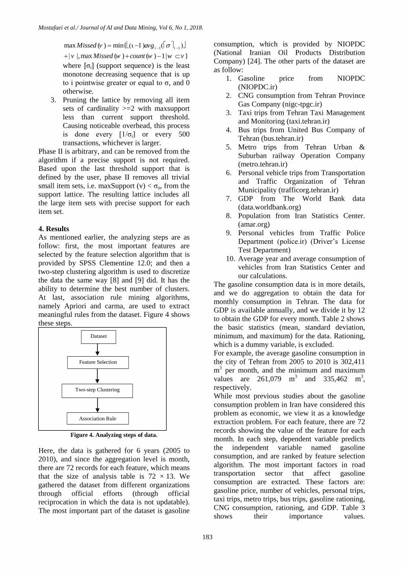
4. Results

As mentioned earlier, the analyzing steps are as

follow: first, the most important features are

selected by the feature selection algorithm that is

provided by SPSS Clementine 12.0; and then a

two-step clustering algorithm is used to discretize

the data the same way [8] and [9] did. It has the

ability to determine the best number of clusters.

At last, association rule mining algorithms,

namely Apriori and carma, are used to extract

meaningful rules from the dataset. Figure 4 shows

these steps.

Figure 4. Analyzing steps of data.

Here, the data is gathered for 6 years (2005 to

2010), and since the aggregation level is month,

there are 72 records for each feature, which means

that the size of analysis table is 72 × 13. We

gathered the dataset from different organizations

through official efforts (through official

reciprocation in which the data is not updatable).

The most important part of the dataset is gasoline

consumption, which is provided by NIOPDC

(National Iranian Oil Products Distribution

Company) [24]. The other parts of the dataset are

as follow:

1. Gasoline price from NIOPDC

(NIOPDC.ir)

2. CNG consumption from Tehran Province

Gas Company (nigc-tpgc.ir)

3. Taxi trips from Tehran Taxi Management

and Monitoring (taxi.tehran.ir)

4. Bus trips from United Bus Company of

Tehran (bus.tehran.ir)

5. Metro trips from Tehran Urban &

Suburban railway Operation Company

(metro.tehran.ir)

6. Personal vehicle trips from Transportation

and Traffic Organization of Tehran

Municipality (trafficorg.tehran.ir)

7. GDP from The World Bank data

(data.worldbank.org)

8. Population from Iran Statistics Center.

(amar.org)

9. Personal vehicles from Traffic Police

Department (police.ir) (Driver’s License

Test Department)

10. Average year and average consumption of

vehicles from Iran Statistics Center and

our calculations.

The gasoline consumption data is in more details,

and we do aggregation to obtain the data for

monthly consumption in Tehran. The data for

GDP is available annually, and we divide it by 12

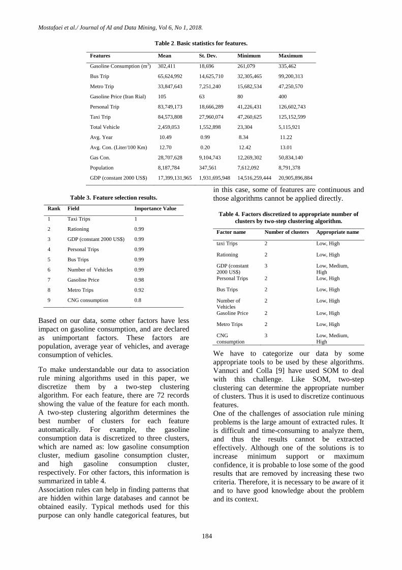
to obtain the GDP for every month. Table 2 shows

the basic statistics (mean, standard deviation,

minimum, and maximum) for the data. Rationing,

which is a dummy variable, is excluded.

For example, the average gasoline consumption in

the city of Tehran from 2005 to 2010 is 302,411

m3 per month, and the minimum and maximum

values are 261,079 m3 and 335,462 m

3,

respectively.

While most previous studies about the gasoline

consumption problem in Iran have considered this

problem as economic, we view it as a knowledge

extraction problem. For each feature, there are 72

records showing the value of the feature for each

month. In each step, dependent variable predicts

the independent variable named gasoline

consumption, and are ranked by feature selection

algorithm. The most important factors in road

transportation sector that affect gasoline

consumption are extracted. These factors are:

gasoline price, number of vehicles, personal trips,

taxi trips, metro trips, bus trips, gasoline rationing,

CNG consumption, rationing, and GDP. Table 3

shows their importance values.

Dataset

Feature Selection

Two-step Clustering

Association Rule


184

Table 2. Basic statistics for features.

Features Mean St. Dev. Minimum Maximum

Gasoline Consumption (m3) 302,411 18,696 261,079 335,462

Bus Trip 65,624,992 14,625,710 32,305,465 99,200,313

Metro Trip 33,847,643 7,251,240 15,682,534 47,250,570

Gasoline Price (Iran Rial) 105 63 80 400

Personal Trip 83,749,173 18,666,289 41,226,431 126,602,743

Taxi Trip 84,573,808 27,960,074 47,260,625 125,152,599

Total Vehicle 2,459,053 1,552,898 23,304 5,115,921

Avg. Year 10.49 0.99 8.34 11.22

Avg. Con. (Liter/100 Km) 12.70 0.20 12.42 13.01

Gas Con. 28,707,628 9,104,743 12,269,302 50,834,140

Population 8,187,784 347,561 7,612,092 8,791,378

GDP (constant 2000 US$) 17,399,131,965 1,931,695,948 14,516,259,444 20,905,896,884

Table 3. Feature selection results.

Rank Field Importance Value

1 Taxi Trips 1

2 Rationing 0.99

3 GDP (constant 2000 US$) 0.99

4 Personal Trips 0.99

5 Bus Trips 0.99

6 Number of Vehicles 0.99

7 Gasoline Price 0.98

8 Metro Trips 0.92

9 CNG consumption 0.8

Based on our data, some other factors have less

impact on gasoline consumption, and are declared

as unimportant factors. These factors are

population, average year of vehicles, and average

consumption of vehicles.

To make understandable our data to association

rule mining algorithms used in this paper, we

discretize them by a two-step clustering

algorithm. For each feature, there are 72 records

showing the value of the feature for each month.

A two-step clustering algorithm determines the

best number of clusters for each feature

automatically. For example, the gasoline

consumption data is discretized to three clusters,

which are named as: low gasoline consumption

cluster, medium gasoline consumption cluster,

and high gasoline consumption cluster,

respectively. For other factors, this information is

summarized in table 4.

Association rules can help in finding patterns that

are hidden within large databases and cannot be

obtained easily. Typical methods used for this

purpose can only handle categorical features, but

in this case, some of features are continuous and

those algorithms cannot be applied directly.

Table 4. Factors discretized to appropriate number of

clusters by two-step clustering algorithm.

Factor name Number of clusters Appropriate name

taxi Trips 2 Low, High

Rationing 2 Low, High

GDP (constant

2000 US$)

3 Low, Medium,

High

Personal Trips 2 Low, High

Bus Trips 2 Low, High

Number of Vehicles

2 Low, High

Gasoline Price 2 Low, High

Metro Trips 2 Low, High

CNG

consumption

3 Low, Medium,

High

We have to categorize our data by some

appropriate tools to be used by these algorithms.

Vannuci and Colla [9] have used SOM to deal

with this challenge. Like SOM, two-step

clustering can determine the appropriate number

of clusters. Thus it is used to discretize continuous

features.

One of the challenges of association rule mining

problems is the large amount of extracted rules. It

is difficult and time-consuming to analyze them,

and thus the results cannot be extracted

effectively. Although one of the solutions is to

increase minimum support or maximum

confidence, it is probable to lose some of the good

results that are removed by increasing these two

criteria. Therefore, it is necessary to be aware of it

and to have good knowledge about the problem

and its context.


185

4.1. Apriori algorithm results

In this sub-section, we will analyze the

relationships between gasoline consumption and

other factors. There is no rule for low gasoline

consumption when the model is run based on

SPSS Clementine 12.0 [27] default settings. To

investigate the changes in other factors that

contribute to low gasoline consumption, we have

to decrease the minimum support. By decreasing

it from 10% to 9%, the following results were

obtained.

Since we have a good sight about our data, to

extract good rules from data, we run the model for

several times and change the minimum support

and the minimum confidence to get good results.

At the end, we set minimum support and

minimum confidence to 9% and 75%,

respectively. It is useful to note that there are three

types of association rules: 1) obvious rules, which

verify both the dataset that is used and the

algorithm. 2) Unexplained rules that have no

meanings. 3) Interesting rules that have to be

extracted for analysis purpose. Here, both obvious

rules and interesting rules are mentioned.

4.1.1. Low gasoline consumption

Table 5 shows the most remarkable rules that are

extracted. Rule 1 says that the low gasoline

consumption between the years 2005 and 2010

was a result of low amounts of vehicles and high

taxi trips. Rule 2 says that low gasoline

consumption was a result of low amount of

vehicles and gasoline rationing. In rule 3, low

amounts of vehicles, high taxi trips, and high

number of bus trips are three reasons of low

gasoline consumption. In rule 4, low amounts of

vehicles, high bus trips, and gasoline rationing are

three reasons of low gasoline consumption. In rule

5, low amounts of vehicles, high taxi trips, and

gasoline rationing are three reasons of low

gasoline consumption. Rule 6 shows that high bus

and taxi trips, rationing, and fewer numbers of

vehicles conquered low gasoline price and caused

low gasoline consumption. Rule 7 is similar to

Rule 2 but it has a low gasoline price in

antecedent that shows that rationing and fewer

number of vehicles neutralized the low gasoline

price and also caused low gasoline consumption.

It has to be mentioned that compared to personal

trips, taxi trips cause low gasoline consumption.

The reason for this is the passenger rate. The

number of passengers that are transported by one

taxi is more than the number transported by

personal vehicles. Accordingly, the overall

gasoline consumption is reduced.

In general, the most important factors that

contributed to the low gasoline consumption were:

low amount of vehicles, high taxi trips, gasoline

rationing, and high number of bus trips.

As a useful result, we can see that taxi trips and

bus trips were a good substitution for personal

trips, which are the main causes of high gasoline

consumption. Thus paying more attention to these

sectors will be helpful in reducing gasoline

consumption.

Table 5. Extracted rules for low gasoline consumption by

Apriori algorithm.

Rule Explanation

1 if number of vehicles =’[2.33E+04,2.30E+06]’∩Taxi

trips=’[8.97E+07, 1.25E+08]’=> class Low (sup.=

%9.72, conf.=1)

2 if number of vehicles =’[2.33E+04,2.30E+06]’∩

Rationing=’True’=> class Low (sup.= %9.72, conf.=1)


trips=’[8.97E+07, 1.25E+08]’∩ Bus trips=’[6.29E+07, 9.92E+07]’=> class Low (sup.= %9.72, conf.=1)

4 if number of vehicles =’[2.33E+04,2.30E+06]’∩

Rationing=’True’ ∩ Bus trips=’[6.29E+07,

9.92E+07]’=> class Low (sup.= %9.72, conf.=1)

5 if number of vehicles =’[2.33E+04,2.30E+06]’∩Taxi trips=’[8.97E+07, 1.25E+08]’∩ Rationing=’True’=>

class Low (sup.= %9.72, conf.=1)


trips=’[8.97E+07, 1.25E+08]’∩ Rationing=’True’ ∩ Gasoline price =’[800,1000]’ ∩ Bus trips=’[6.29E+07,

9.92E+07]’=> class Low (sup.= %9.72, conf.=1)s

7 if number of vehicles =’[2.33E+04,2.30E+06]’ ∩ Gasoline price =’[800,1000]’ ∩ Rationing=’True’=>

class Low (sup.= %9.72, conf.=1)

4.1.2. Medium gasoline consumption

Low gasoline consumption occurred after

rationing, and high gasoline consumption

occurred before rationing but this cluster occurred

throughout the whole period and, compared to two

other clusters, is of less interest to be analyzed.

Due to its spread throughout the whole period,

there are lots of rules in this case. Table 6 shows

three important rules as the cause of Medium

gasoline consumption.

Rule 1 says that although we had a high number

of vehicles and numerous personal trips, medium

CNG consumption prevented an increase in

gasoline consumption. Rule 2 says that the high

number of trips by metro and bus prevented

gasoline consumption from increasing. Rule 3

shows that although we had high CNG

consumption, all impacts of this is arbitrated by


186

the factors such as high number of metro trips,

numerous taxi trips, and low gasoline price.

One of the interesting results is that medium

gasoline consumption occurred with high CNG

consumption. It implies that replacing CNG in the

road transportation sector was not enough to

reduce gasoline consumption, and other strategies

are required to address this issue.

Table 6. Extracted rules for medium gasoline

consumption by Apriori.

Rule Explanation

1 if CNG consumption =’[2.47E+07,3.49E+07]’ ∩ Personal

trips = ‘[4.12E+07,7.58E+07]’ ∩ number of vehicles =’[2.39E+06,5.12E+06]’ ∩ Bus trips=’[6.29E+07,

9.92E+07]’ ∩ Rationing=’True’=> class Medium (sup.=

%9.72, conf.=1)

2 if CNG consumption =’[2.47E+07,3.49E+07]’ ∩ Personal trips = ‘[4.12E+07,7.58E+07]’ ∩ number of vehicles

=’[2.39E+06,5.12E+06]’∩ Bus trips=’[6.29E+07, 9.92E+07]’∩ Metro trips=’[3.32E+07, 4.73E+07]’ => class

Medium (sup.= %9.72, conf.=1)

3 if CNG consumption =’[3.81E+07,5.08E+07]’ ∩ Metro

trips=’[3.32E+07, 4.73E+07]’ ∩Rationing=’True’ ∩Taxi trips=’[8.97E+07, 1.25E+08]’∩ Gasoline price

=’[800,1000]’=> class Medium (sup.= %9.72, conf.=1)

4.1.3. High gasoline consumption Table 7 shows the rules extracted for this cluster.

Rule 1 shows that due to the low gasoline price

and high number of trips by personal vehicles, the

gasoline consumption was high. By lowering the

minimum confidence, an interesting rule was

obtained. It conveys that low gasoline price, high

personal trips, fewer metro and taxi trips

culminated in high gasoline consumption.

Table 7. Extracted rules for high gasoline consumption.

Rule Explanation

1 if Taxi trips =’[4.73E+07, 5.42E+07]’ ∩ CNG consumption =’[2.47E+07,3.49E+07]’ ∩ Personal trips =

‘[8.03E+07,1.27E+08]’ ∩ Gasoline price =’[800,1000]’=>

class High (sup.= %16.67, conf.=.83) 2 if Taxi trips =’[4.73E+07, 5.42E+07]’ ∩ Metro trips

=’[1.57E+07, 3.26E+07]’ ∩ CNG consumption =

’[2.47E+07,3.49E+07]’∩Personal trips = ‘[8.03E+07, 1.27E+08]’ ∩ => class High (sup.= %16.67, conf.=.83)

3 if Taxi trips =’[4.73E+07, 5.42E+07]’ ∩ Gasoline price

=’[800,1000]’ ∩ number of vehicles =’ [2.33E+04,2.30E+06]’ ∩ CNG consumption = ’[2.47E+07,3.49E+07]’∩Personal trips = ‘[8.03E+07,

1.27E+08]’ ∩ => class High (sup.= %16.67, conf.=.83)

Rule 1 shows that a low gasoline price has a direct

effect on the high gasoline consumption. Also

according to rule 2, high personal trips have the

direct effect of low gasoline price. Thus as a

result, it can be implied that a low gasoline price

is the most important factor in a high gasoline

consumption. Rule 3 implies that although there

were medium CNG consumption and fewer

number of vehicles, high personal trips, fewer taxi

trips, and low gasoline price caused a high

gasoline consumption.

4.2. Carma algorithm results

In this section, we analyze the associations

between gasoline consumption and other factors

by Carma algorithm after removing unimportant

factors.

The Carma algorithm has the advantage of

assuming each factor as the subsequent part of

association rule mining algorithms and works as

follows: each time, it takes one of the factors as a

dependent factor and examines the effects of other

factors on that factor. This makes it possible to be

aware of all changes that occur in this area.

Table 8. Extracted rules by Carma algorithm.

Rule Explanation

1 if Rationing=’True’=>Taxi trips=’[8.97E+07,

1.25E+08]’(sup.= %62.5, conf.=1)

2 if number of vehicles =’[2.33E+04,2.30E+06]’=> Bus

trips=’[6.29E+07, 9.92E+07]’ (sup.= %47.2, conf.=1)

3 if Rationing=’True’=> Metro trips=’[3.32E+07, 4.73E+07]’ (sup.= %62.5, conf.=.91)

4 if Rationing=’True’=> Metro trips=’[3.32E+07,

4.73E+07]’ ∩Taxi trips=’[8.97E+07, 1.25E+08]’ (sup.= %62.5, conf.=.91)

5 if Gasoline price =’[800,1000]’ ∩ number of vehicles

=’[2.39E+06,5.12E+06]’ ∩ Metro trips=’ [1.57E+07,

3.26E+07]’ ∩Taxi trips=’ [4.73E+07, 5.42E+07]’ =>’ Personal trips = ‘[8.03E+07,1.27E+08]’ (sup.= %31.94,

conf.=1)

To compare the results of the two algorithms, we

set the minimum support and minimum

confidence to 9% and 75%, respectively. There

are lots of results obtained through these settings.

These results showed that the Carma algorithm

can extract all rules that were extracted by the

Apriori algorithm. Some of the important results,

other than those explained at the Apriori

algorithm results, are shown in table 8.

Rule 1 shows one of the interesting rules that

rationing has a strong effect on the increase in the

taxi trips. It means that, by rationing gasoline

consumption, there was not enough gasoline for

personal vehicle owners to accommodate the past

behavior, and instead, they used taxi for traveling.

Rule 2 implies that in those years that there were

less personal vehicles, people used bus more than

other three means of transportation. Rule 3 shows

that gasoline rationing caused metro trips to


187

increase. This is an important event because in the

long term, it has benefits for both the people and

the government.

It reduces gasoline consumption, which is

favorable for the government. It also speeds up

trips and reduces traffic jams in the streets, which

is favorable for the people. Rule 4 shows that

rationing also caused taxi trips to increase. Rule 5

shows that there are fewer vehicles but low

gasoline price and fewer number of trips done by

public transportation are caused high personal

trips.

Taxi trips, bus trips, and metro trips are three

substitutions for personal trips to reduce gasoline

consumption. We showed that the first and rapid

effect of gasoline rationing was on increasing taxi

trips. Bus trips also increased but this increase

was less than increasing in taxi trips. Therefore,

taxi trips and bus trips can be considered as a

short-term solution for decreasing the gasoline

consumption. By expanding metro through these

years, there was a continuous increase in metro

trips.

Figure 5 shows metro trips for the city of Tehran

from 2005 to 2010. Actually the usage of metro

for transportation was at the highest level after

gasoline rationing. Since expanding of the metro

requires a lot of investment, it should be seen as a

long-term solution for decreasing the gasoline

consumption.

Figure 5. Monthly metro trips for city of Tehran.

4.3. Statistical correlation analysis

Here, statistical correlation analysis is performed

on all features. One of the common approaches to

examine the correlation between features is the

Pearson’s coefficient, which was introduced by

Karl Pearson [30]. A perquisite to the Pearson’s

coefficient is that all features have to be normal.

Since rationing is a dummy variable, the data is

divided into two parts, i.e. before rationing and

after rationing, and these two parts are analyzed

separately. Here, the confidence level is set to

0.95. It is shown in table 9 and table 10; all

features are not normal (p-value less than 0.05),

and therefore, the Pearson’s coefficient cannot be

used. Non-parametric equivalent test to Pearson is

the spearman test, which is used here to test the

data. The results obtained are shown in table11

and table 12 for the spearman correlation

coefficient between features before rationing and

after rationing, respectively.

Table 9. Normality test for data before rationing.

Mean StDev P-Value

Gasoline Con. 314532 15464 0.165

Bus Trip 77644477 7526330 0.251

Metro Trip 26330675 4958841 0.253

Personal Trip 99089958 9606059 0.251

Taxi Trip 50577086 2280905 0.164

Total Vehicle 770611 528460 0.227

Avg. Year 11.08 0.1317 <0.005

Avg. Con. 12.91 0.09329 <0.005

Gas Con. 22405834 5827351 0.329

Population 7816487 125857 0.584

GDP 1.54E+10 7.77E+08 <0.005

Table 10. Normality test for data after rationing.

Mean St. Dev. P-Value

Gasoline Con. 295138 16688 0.013

Bus Trip 120 75.68 <0.005

Metro Trip

58413301

1303309

0 0.006

Personal Trip 38357824 3851987 0.244

Taxi Trip 74544702

16632864 0.006

Total Vehicle

1.05E+08

1111972

9 0.037 Avg. Year

3472118 962936 0.387 Avg. Con.

10.14 1.104 <0.005 Gas Con.

12.57 0.1205 <0.005 Population

32488705 8643372 <0.005

GDP 8410563 224075 0.22

As it can be seen in table 11, metro trips and taxi

trips have a strong correlation because the use of

these two public transportation sectors increases

over the time. Although the correlation between

average year of vehicles and metro trips are

negatively strong, it cannot be implied that they

are meaningfully correlated. The correlation

between metro trips and population is obvious.


188

Table 11. Spearman’s correlation coefficient before rationing.

Features Gasoline Con.(m3) Bus

Trip

Metr

o

Trip

Person

al Trip

Taxi

Trip

Total

Vehic

le

Av.

Year

Avg.

Con.

Gas

Con.

Population

Bus Trip 0.48

Metro Trip 0.36 0.27

Personal Trip 0.48 1.00 0.27

Taxi Trip 0.18 0.03 0.91 0.1

Total Vehicle 0.20 0.05 0.91 0.9 1.00

Avg. Year -0.27 -0.20 -0.81 -0.2 -0.86 -0.86

Avg. Con. -0.23 -0.12 -0.81 -0.12 -0.91 -0.91 0.95

Gas Con. 0.30 0.26 0.83 0.26 0.83 0.83 -0.82 -0.81

Population 0.20 0.05 0.91 0.83 1.00 1.00 -0.86 -0.91 0.83

GDP 0.20 0.05 0.91 0.83 1.00 1.00 -0.86 -0.91 0.83 1.00

The reason for high correlation between average

consumption of vehicles and average year of

vehicles is that these two features are decreasing

over the period because of revitalizing of vehicles.

One other obvious result is that due to the low

gasoline price, there is a positive correlation

between the number of vehicles and the personal

trips before rationing.

Table 12. Spearman’s correlation coefficient after rationing.

Features Gasoline Con. (m3) Gasoline

Price

Bus

Trip

Metro

Trip

Perso

nal

Trip

Taxi

Trip

Total

Vehi

cle

Avg.

Year

Avg.

Con.

Gas

Con.

Population

Gasoline

Price -0.21

Bus Trip -0.09 -0.29

Metro Trip 0.34 0.43 -0.15

Personal Trip -0.09 -0.29 1 -0.15

Taxi Trip -0.25 -0.25 0.78 -0.29 -0.87

Total Vehicle 0.25 0.43 -0.88 0.50 -0.52 -0.87

Avg. Year -0.26 -0.35 0.86 -0.41 0.63 0.97 -0.97

Avg. Con. -0.26 -0.35 0.86 -0.41 0.63 0.97 -0.97 1

Gas Con. 0.09 0.23 -0.74 0.43 -0.24 -0.78 0.86 -0.85 -0.85

Population 0.25 0.43 -0.88 0.50 0.21 -0.87 1 -0.97 -0.97 0.86

GDP 0.25 0.43 -0.88 0.50 0.21 -0.87 1 -0.97 -0.97 0.86 1

As shown in table 12, there is a significant

correlation between bus trips and taxi trips, and it

can be due to the fact that despite an increase in

the use of these two public transportation sectors,

there is no significant correlation between metro

trips and these two sectors. Taxi trips have a

negative correlation with the number of vehicles,

which means that as people buy their own car,

they use it for the transportation purposes. Taxi

trips also have a negative correlation with the

CNG consumption, and since the CNG

consumption and the number of vehicles are

positively strongly correlated, it can be implied

that the reason for the increase in the CNG

consumption can increase with the number of

vehicles. One of the interesting results is that there

is a negatively strong correlation between the

personal trips and the taxi trips, which implies that

some fractions of the personal trips are replaced

by taxi trips.

5. Conclusion

In this work, we investigated the major changes

that have occurred in the road transportation

sector from March 2005 to March 2011. Since

July 2007, gasoline consumption has been

rationed. For this purpose, we used the association

rule mining algorithms such as Apriori and

Carma, which are supported by SPSS Clementine

12.0. These results were compared with the

statistical correlation analysis. The comparison

results showed that the association rule mining

algorithms could obtain complicated rules than the

statistical correlation analysis. This study is

special for its viewpoint. In spite of other studies

that used economical techniques to analyze the


189

gasoline consumption trend, the association rule

mining algorithms were used to investigate the

relationships among the gasoline consumption and

other features in the road transportation sector that

have effect on it. Due to the low gasoline price, its

consumption grew rapidly during 2005 and 2006.

To stop its growth, gasoline was rationed in July

2007, and, in addition to this, the government

tried to increase the CNG consumption and

expand metro. The association rule mining

algorithm results showed that there was no

significant rule for impact of CNG consumption

on the gasoline consumption reduction. A rapid

increase in the number of people using public

transportation system especially taxi, is an

indication of gasoline rationing in the road

transportation sector. The reason is that taxi is

more available than the other means of public

transportation sectors. Therefore, it can be as a

short-term solution for the transportation problem.

Another impact of gasoline rationing was the

increase in the passengers of metro. This increase

has continued after gasoline rationing so it can be

a long-term solution for handling the

transportation demand. By comparing the results

obtained from both the Apriori and Carma

algorithms, we showed that the Carma algorithm

also yields those results obtained from the Apriori

algorithm.

References [1] Taraznameh, Balance report in.

[2] Khan, M. S., Muyeba, M., & Coenen, F. (2008). A

weighted utility framework for mining association

rules. EMS 2008, Second UKSIM European

Symposium on Computer Modeling and Simulation.

Liverpool, England, UK, 2008.

[3] Chalaris, M., Chalaris, I., Skourlas, C., &

Tsolakidis, A. (2013). Extraction of rules based on

students’ questionnaires. Procedia-Social and

Behavioral Sciences, vol. 73, pp. 510-517.

[4] Abdullah, Z., Herawan, T., Ahmad, N., & Deris, M.

M. (2011). Mining significant association rules from

educational data using critical relative support

approach. Procedia-Social and Behavioral Sciences,

vol. 28, pp. 97-101.

[5] Nair, A. K., Sugunan, D., Kumar, H., & Anilkumar,

G. (2012). Association analysis of common variants in

FOXO3 with type 2 diabetes in a South Indian

Dravidian population. Gene, vol. 491, no. 2, pp. 182-

186.

[6] Kousa, A., Puustinen, N., Karvonen, M., &

Moltchanova, E. (2012). The regional association of

rising type 2 diabetes incidence with magnesium in

drinking water among young adults. Environmental

research, vol. 112, pp. 126-128.

[7] Nahar, J., Imam, T., Tickle, K. S., & Chen, Y. P. P.

(2013). Association rule mining to detect factors which

contribute to heart disease in males and females. Expert

Systems with Applications, vol. 40, no. 4, pp. 1086-

1093.

[8] Taboada, K., Shimada, K., Mabu, S., Hirasawa, K.,

& Hu, J. (2007). Association rules mining for handling

continuous attributes using genetic network

programming and fuzzy membership functions. SICE

Annual Conference 2007, Kagawa, Japan, 2007.

[9] Vannucci, M & Colla, V. (2004). Meaningful

discretization of continuous features for association

rules mining by means of a SOM. 12th European

Symposium on Artificial Neural Networks, Bruges,

Belgium, 2004.

[10] Jafari, H. H., & Baratimalayeri, A. (2008). The

crisis of gasoline consumption in the Iran's

transportation sector. Energy Policy, vol. 36, no. 7, pp.

2536-2543.

[11] Ahmadian, M., Chitnis, M., & Hunt, L. C. (2007).

Gasoline demand, pricing policy and social welfare in

Iran. Surrey Energy Economics Centre (SEEC), School

of Economics, University of Surrey. vol. 31, no. 2, pp.

105-124.

[12] Sharify, N. (2009). An assessment of quota in

gasoline consumption in Iran: an AGE Approach. The

17th International Conference on Input-Output

techniques, University of São Paulo, São Paulo,

Brazil., 2009.

[13] Sarabi, E. R. (2011). An analysis to energy

consumption rate in road transportation sector of Iran

and introduction policies of fuel consumption

management in recent years. Procedia Engineering,

vol. 21, pp. 989-996.

[14] Meibodi, A. E., & Aalami, R. (2011). Gasoline

Consumption Analysis of the vehicles in Developing

Countries by Multiplicative LMDI Approach: The case

of Iran. International Conference On Applied

Economics–ICOAE, Perugia, Italy, 2011.

[15] Azadeh, A., Manzour Alajdad, S. M. H., &

Aliheidari Bioki, T. (2014). A neuro-fuzzy regression

approach for estimation and optimisation of gasoline

consumption. International Journal of Services and

Operations Management, vol. 17, no. 2, pp. 221-256.

[16] Azadeh, A., Behmanesh, I., Vafa Arani, H., &

Sadeghi, M. H. (2014). An integrated fuzzy

mathematical programming-analysis of variance

approach for forecasting gasoline consumption with

ambiguous inputs: USA, Canada, Japan, Iran and

Kuwait. International Journal of Industrial and Systems

Engineering, vol. 18, no. 2, pp.n159-184.

[17] Moshiri, S., & Aliyev, K. (2017). Rebound effect

of efficiency improvement in passenger cars on

gasoline consumption in Canada. Ecological

Economics, vol. 131, pp. 330-341.


190

[18] Alavi, S. A. R., & Abunoori, A. A. (2015).

Modelling and Estimating Gasoline Demand Using

AIDS for Urban Low-Income Groups. European

Online Journal of Natural and Social Sciences, vol. 4,

no. 1(s), pp. 625-634.

[19] Taghvaee, V. M., & Hajiani, P. (2014). Price and

income elasticities of gasoline demand in Iran: using

static, ECM, and dynamic models in short,

intermediate, and long run. Modern Economy, vol. 5,

pp. 939-950.

[20] Agrawal, R., Imieliński, T., & Swami, A. (1993).

Mining association rules between sets of items in large

databases. In Acm sigmod record, vol. 22, no. 2, pp.

207-216.

[21] Song, Y. C., & Fang, Y. F. (2010). Application

research of association analysis with Clementine. 2010

2nd International Conference on Software Engineering

and Data Mining (SEDM). Chengdu, China. 2010.

[22] Woon, Y. K., Ng, W. K., & Lim, E. P. (2001).

Association rule mining for electronic commerce: New

challenges. ICICS‘01, Third International Conference

on Information, Communications & Signal Processing .

Singapore , Singapore, 2001.

[23] Huang, Y., Wang, X., & Shia, B. C. (2009,

August). Efficiency and Consistency Study on Carma.

NCM 2009: 5th INTERNATIONAL JOINT

CONFERENCE on INC, IMS and IDC. Seoul, Korea,

2009.

[24] The National Iranian Oil Products Distribution

Company (2017), Available: http://niopdc.ir/.

[25] Chiu, T., Fang, D., Chen, J., Wang, Y., & Jeris, C.

(2001). A robust and scalable clustering algorithm for

mixed type attributes in large database environment.

KDD '01 ACM SIGKDD International Conference on

Knowledge Discovery and Data Mining, San

Francisco, CA, USA, 2001.

[26] Hidber, C. (1999). Online association rule mining.

ACM, vol. 28, no. 2, pp. 145-156.

[27] Clementine, S. P. S. S. (2007). 12.0 Algorithm

Guide. Chicago, USA, 2007.

[28] Zahedi, F., Zare-Mirakabad, M. R. (2014).

Employing data mining to explore association rules in

drug addicts, language, Journal of AI and Data Mining,

Shahroud university , vol. 2, no. 2, pp. 135-139.

نشرهی هوش مصنوعی و داده کاوی

بندی بنزیننگرش جدید به تحلیل سهمیه

2رضا قدسی و 1حامد شکوری گنجوی، ،*1سعید مصطفایی

.ایران، تهران، دانشگاه تهراندانشکده مهندسی صنایع، ، گروه مهندسی صنایع 2و1

.نکتیکات مرکزی، کنکتیکات، آمریکاک ایالتیدانشکده فنی، دانشگاه 3

90/90/6902 پذیرش؛ 62/00/6902 بازنگری؛ 62/90/6902 ارسال

چکیده:

مورد بررسی و تحلیل قرار گرفته است. در حالی که بیشتر مطالعاا 0830تا 0830ای از سال در این کار روابط بین متغیرهای بخش حمل و نقل جاده

دار باین ایان کاوی سعی در استخراج روابط معنایهای دادهاند، در این کار با یک نگرش متفاو و با تکنیکمصرف بنزین داشتهقبلی نگرش اقتصادی به

آوری شاده اسات. ابتادا میازا تاا یر های مختلا جما هاا از ساازما ترین متغیر مورد بررسی مصرف بنزین بوده اسات. دادهمتغیرها شده است. مهم

هاا حاذف بر روی مصرف بنزین به کمک الگوریتم انتخاب ویژگی بدست آمده است. برخی از این متغیرها باه دلیال تاا یر کام از تحلیلمتغیرهای دیگر

ایان دو دو الگوریتم قوانین انجمنی اپریوری و کارما برای تحلیل روابط استفاده شده اسات. .جمعیت، متوسط عمر خودرو و متوسط مصرف اند مانندشده

ساازی اساتفاده شاده اسات. نتاای ای برای گسستهبندی دو مرحلهم قابلیت کار با متغیرهای پیوسته را ندارند، به همین خاطر از الگوریتم خوشهالگوریت

تاای بندی بنزین و سفرهای زیاد انجام شده با تاکسی دلیل اصلی مصرف کم بنازین باوده اسات. نقوانین انجمنی نشا داد که تعداد کم خودرو، سهمیه

گیر داشاته اسات. همیناین نتاای دو الگاوریتم بندی بنزین افزایش چشمالگوریتم کارما نشا داد که تعداد سفرهای انجام شده با تاکسی بعد از سهمیه

شاده اسات کاه نتاای دهد. در آخر نیز نشاا دادهنشا داد که الگوریتم کارما تمامی قوانینی که توسط الگوریتم اپریوری بدست آمده بود را نتیجه می

تر است.های آماری جام قوانین انجمنی نسبت به تحلیل

.کارما قوانین انجمنی، اپریوری،کاوی، بندی بنزین، دادهمصرف بنزین، سهمیه :کلمات کلیدی

new approaches to analyze gasoline...

Documents