neuronal current fmri: pushing the limits of mr-based functional ... · universita degli studi di...
TRANSCRIPT
Universita degli Studi di Roma “La Sapienza”
PhD Thesis in Biophysics
Neuronal current fMRI: pushing thelimits of MR-based functional
neuroimaging
Supervisors:
prof. Bruno Maraviglia
dott. Gisela Hagberg
Student:
Marta Bianciardi
PhD Coordinator:
prof. Alfredo Colosimo
XVII cycle (2001/2004)

Contents
Introduction 2
1 Physiology of cerebral activation by available techniques 7
1.1 Organization of the cerebral cortex: from anatomical to fun-
ctional mapping . . . . . . . . . . . . . . . . . . . . . . . . . . 9
1.2 Electro-physiology of cortical field activation . . . . . . . . . . 10
1.2.1 Stimuli information coding: from receptors to cortex . 10
1.2.2 Cortical input/output and intra-cortical processing . . 13
1.2.3 Neural basis of intra-cortical, EEG and MEG recor-
dings and main findings . . . . . . . . . . . . . . . . . 16
1.3 The metabolic-hemodynamic response associated with cortical
field activation . . . . . . . . . . . . . . . . . . . . . . . . . . 21
1.3.1 The neuro-vascular coupling: blood flow may be con-
trolled by energy demand or by neural signaling . . . . 22
1.3.2 Controversies regarding the locus of cerebral energy use
and of the type of metabolism . . . . . . . . . . . . . . 24
1.3.3 The dynamics of oxygen delivery, blood flow and blood
volume: the physiological model for the BOLD effect . 30
1.4 The neuro-vascular coupling and fMRI signals may reflect sy-
naptic rather than spiking activity . . . . . . . . . . . . . . . . 38
2 Neuronal current fMRI, proposal for an alternative approach
to BOLD fMRI 41
2.1 NMR signal in the brain without contrast agents . . . . . . . . 42
2.2 The effect of endogenous contrast agents on the NMR signal . 44
2.3 A bio-physical model for BOLD MR effects during cerebral
activation . . . . . . . . . . . . . . . . . . . . . . . . . . . . . 48
2.4 Mapping brain function by conventional BOLD-based fMRI
approaches: advantages and limitations . . . . . . . . . . . . . 56
III
IV Contents
2.5 Neuronal current magnetic effects on cerebral MR signal du-
ring activation . . . . . . . . . . . . . . . . . . . . . . . . . . . 58
2.6 Potential benefits and shortcomings of neuronal current fMRI 66
3 Optimization of neuronal current fMRI sensitivity on a phan-
tom 69
3.1 MRI sensitivity for the detection of nTesla magnetic field changes 70
3.2 Multi- versus single-echo approaches with respect to MR sen-
sitivity . . . . . . . . . . . . . . . . . . . . . . . . . . . . . . . 72
3.2.1 Phase stability, theoretical predictions . . . . . . . . . 72
3.2.2 Phase stability on a phantom . . . . . . . . . . . . . . 75
3.3 Acquisition rates and coil types with respect to MR sensitivity 77
3.3.1 Influence on SNR, theoretical expectations . . . . . . . 77
3.3.2 Results on a phantom and in vivo . . . . . . . . . . . . 78
3.4 Detection limit of current induced magnetic effects at 1.5 Tesla
with optimized detection . . . . . . . . . . . . . . . . . . . . . 79
3.5 Discussion and conclusions . . . . . . . . . . . . . . . . . . . . 81
Materials and Methods . . . . . . . . . . . . . . . . . . . . . . 82
4 Neuronal current fMRI of in vivo visual evoked activity 87
4.1 Neuronal current fMRI contrast optimization . . . . . . . . . . 88
4.2 In vivo feasibility of neuronal current fMRI . . . . . . . . . . . 90
4.2.1 Spontaneous versus evoked activity . . . . . . . . . . . 90
4.2.2 Spin- versus gradient-echo techniques . . . . . . . . . . 92
4.3 Overview of the proposed approaches . . . . . . . . . . . . . . 93
4.3.1 The VEP-fMRI approach for synchronizing the neu-
ronal event with SE MR measurements . . . . . . . . . 94
4.3.2 Methods for constraining unwanted signal changes of
non-neuronal origin . . . . . . . . . . . . . . . . . . . . 97
4.4 In vivo MRI detection of visual evoked neuronal current mag-
netic effects . . . . . . . . . . . . . . . . . . . . . . . . . . . . 99
4.5 Discussion and conclusions . . . . . . . . . . . . . . . . . . . 102
Materials and Methods . . . . . . . . . . . . . . . . . . . . . . 106
5 Conclusions and perspectives 113
References 117

Introduction
Since its inception a decade ago, functional MRI (fMRI) has constituted a
revolutionary approach to study brain function because of its several advan-
tages with respect to other imaging modalities. The advent of fMRI has
enabled the investigation of sensory-motor and cognitive processes with a
nominal spatial and temporal resolution of a few mm and hundreds of ms,
respectively, by the use of non-ionizing radiation and with the possibility to
repeat the measurements on the same subject.
The blood oxygenation level dependent (BOLD) effect developed most be-
tween other fMRI strategies, due to its greater availability on clinical scanners
and to the possibility of acquiring slices of the whole brain in few seconds.
Nevertheless, it soon became clear that the actual resolutions of fMRI, and
specially of BOLD fMRI, are limited by the specificity of the BOLD contrast
itself, which is based on secondary rather than direct effects of neuronal ac-
tivity. Blurring in time and space due to the hemodynamic response takes
place and this limitation was evident since the first studies.
Five years ago, the idea of directly measuring neuronal effects by MRI made
it’s debut and a few groups started with investigating the feasibility of de-
tecting such primary neuronal magnetic effects in vivo.
This forthcoming functional contrast may represent an appealing alternative
to conventional blood-oxygen level dependent (BOLD) methods. Neuronal
currents may give more precise temporal information than the sluggish hemo-
dynamic response, since local magnetic field effects vanish as the neuronal
event ceases. Likewise, more precise spatial information may be obtained
since local field variations fall off with the square power of the distance to the
dipolar source, while the BOLD effect may extend to adjacent non-activated
brain areas.
Some early studies [166–168, 170, 171] suggested the feasibility in vitro and
in vivo of the neuronal current fMRI technique. Nevertheless, in this tempt-
ing panorama, some issues are still of intense debate, such as optimization
of the acquisition strategy for detection of neuronal magnetic effects and the
1

2 Introduction
practicability of detecting them in vivo robustly.
In this PhD thesis, we cover these aspects involved in neuronal current fMRI
and propose some solutions. Why should you read this PhD thesis?
..if you are interested in the basics of the electro-physiological and metabolic-
hemodynamic responses which constitute the functional brain response to an
external stimulus as measured by current investigation approaches (Chap. 1).
...if you are interested in the bio-physics at the origin of the BOLD and neu-
ronal current fMRI contrast (Chap. 2).
...if you would like to know what is the detection limit of MRI for ultra-weak
magnetic field changes and how this limit may be pushed down (Chap. 3).
...if you are wondering whether it is possible to detect in vivo primary mag-
netic neuronal effects by MRI (Chap. 4).
With this advice, we only remark here and then soon conclude that we believe
it is worth dwelling on new ideas and exploring the theoretical and exper-
imental limits of the current knowledge, even when those ideas sometimes
may seem “crazy”, unpopular and may be actually troublesome. We hope
that in the future more time and funds will be spent for scientific research
at the cutting-edge, especially in Italy.

Acronyms 3
Mathematical Notation
a The bold typeface in equations indicates a vector (for MR
signal a vector in the complex space).
A+, a+ + is the pseudo-inverse operator of matrix A and of a vector
a, respectively (e.g., for the former, equal to (ATA)−1AT ,
with T equal to the transpose operator).
Re(a) , Im(a) Real and imaginary part of the complex vector a, respective-
ly.∑k Abbreviated notation for the average value ( 1
N
∑Nk=1) over
all the spins (or spin packets) k in a voxel (sometimes
abbreviated as <>).
min(a, b) Minimum value between the two scalars a and b.
Acronyms frequently used in the text
AFNI Analysis of functional neuro-images tool
ANLS Astrocyte-neuron lactate shuttle
ATP Adenosine 5′-triphosphate
BA Brodmann area
BESA Brain electrical source analysis
BL Blood
BOLD Blood oxygen level dependent
BW Bandwidth
CO2a/cArterial/capillary oxygen concentration
CBF Cerebral blood flow
CBV Cerebral blood volume
CSF Cerebro-spinal fluid
CMRglc Cerebral metabolic rate of glucose
CMRO2 Cerebral metabolic rate of oxygen
CNR Contrast to noise ratio
CT Computerized tomography
dHb Deoxyhemoglobin
D Diffusion coefficient
E Oxygen extraction fraction
ECD Equivalent current dipole
4 Acronyms
EEG Electro-encephalography
EP/F Evoked potential/field
EPI Echo-planar imaging
E/IPSP Excitatory/Inhibitory post-synaptic potential
ERP/F Event-related potential/field
EV Extravascular
Fin/out Flow in/out
FIR Finite impulse response
fMRI Functional magnetic resonance imaging
FOV Field of view
FWHM Full width half maximum
GE Gradient echo
G/WM Gray/white matter
Hb Hemoglobin
HbO2 Oxyhemoglobin
IV Intravascular
LD Diffusion length
LDF Laser doppler flowmetry
LFP Local field potential
mEFP Mean extra-cellular field potential
MEG Magneto-encephalography
MRI Magnetic resonance imaging
MR Magnetic resonance
MRS Magnetic resonance spectroscopy
MUA Multiple-unit activity
NIRS Near infrared spectroscopy
NMR Nuclear magnetic resonance
OEF Oxygen extraction fraction
OTT Oxygen transport to tissue
PET Positron emission tomography
PC Purkinje cell
PF Parallel fiber
Q Coil quality factor
RBC Red blood cell
RF Radiofrequency
SE Spin echo
SNR Signal to noise ratio
SPECT Single photon emission computed tomography
SPM Statistical parametric mapping

Acronyms 5
SQUID Super-conducting quantum interference device
SSP/F Steady state potential/field
TE Echo time
TR Repetition time
Veff Effective volume
VEP Visual evoked responses
Vv Venous volume
vvox Voxel volume


Chapter 1
Physiology of cerebral
activation and mapping of brain
function by available techniques
The investigation of brain anatomy and function is one of the most challeng-
ing topics of the 19th and of the 20th centuries and is still an issue of current
research.
Owing to the development of technology for the study of the brain over the
past century, the picture of the cerebral cortex has changed considerably. The
first cortical representation was anatomically driven. At the beginning of the
century, it was developed through the use of staining methods ex vivo. It was
later extended and applied in vivo by the advent of techniques such as com-
puterized axial tomography (CT) and magnetic resonance imaging (MRI).
Conversely, the delineation of a detailed brain functional organization in
vivo, in terms of functional maps, is the fascinating result, still incomplete,
of studies performed primarily in the past three decades. It constitutes a
complementary but not always overlapping picture of the anatomical repre-
sentation of the cortex; moreover, in terms of functional maps, it has been
delineated by the use of several methods sensitive to physiological changes
associated with cerebral activation. Remarkable is the pioneering work of
Broca in the middle of the 19th century [1], which can be considered the first
evidence supporting the existence of a regional functional specialization of
the human cortex: indeed, through the analysis of an ex vivo brain, he linked
an impairment of function to a lesion, that is, to a well localized cerebral re-
gion.
Nevertheless, cerebral activation itself, which occurs in a well localized brain
7
8
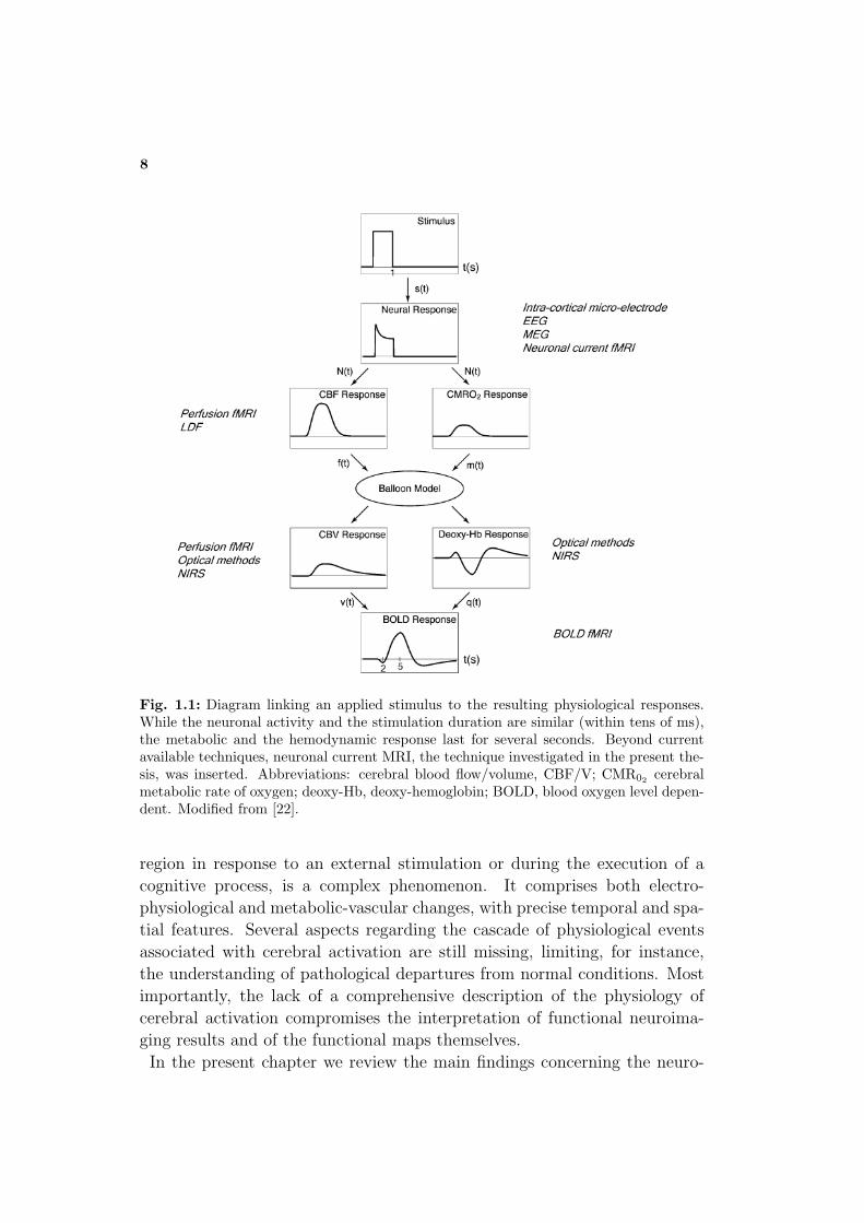
Fig. 1.1: Diagram linking an applied stimulus to the resulting physiological responses.While the neuronal activity and the stimulation duration are similar (within tens of ms),the metabolic and the hemodynamic response last for several seconds. Beyond currentavailable techniques, neuronal current MRI, the technique investigated in the present the-sis, was inserted. Abbreviations: cerebral blood flow/volume, CBF/V; CMR02 cerebralmetabolic rate of oxygen; deoxy-Hb, deoxy-hemoglobin; BOLD, blood oxygen level depen-dent. Modified from [22].
region in response to an external stimulation or during the execution of a
cognitive process, is a complex phenomenon. It comprises both electro-
physiological and metabolic-vascular changes, with precise temporal and spa-
tial features. Several aspects regarding the cascade of physiological events
associated with cerebral activation are still missing, limiting, for instance,
the understanding of pathological departures from normal conditions. Most
importantly, the lack of a comprehensive description of the physiology of
cerebral activation compromises the interpretation of functional neuroima-
ging results and of the functional maps themselves.
In the present chapter we review the main findings concerning the neuro-

1. Physiology of cerebral activation by available techniques 9
physiological response to an external sensory stimulation, based on currently
available functional investigation techniques. Among these techniques, ap-
proaches measuring electro- and magneto-encephalographic changes underly-
ing cerebral activation (both Electro- and Magneto-EncephaloGraphy, EEG
and MEG, on scalp, and intracellular micro-electrode recordings) can be dis-
tinguished from methods detecting changes in the metabolic and in the vascu-
lar cerebral response. The latter methods can be further grouped according to
the employed apparatus, into Magnetic Resonance techniques (functional MR
imaging, fMRI, and MR spectroscopy, MRS), nuclear medicine approaches
(Positron Emission Tomography, PET, and Single Photon Emission Com-
puted Tomography, SPECT) and optical approaches (measurement of intrisic
signals, Laser Doppler Flowmetry, LDF, and Near InfraRed Spectroscopy,
NIRS). Comments on the performance and functioning of each technique are
given throughout the chapter, with particular attention to EEG, MEG and
fMRI strategies. In Fig. 1.1 we depict in a schematic view the time-course of
some electro-physiological and metabolic parameters measurable by current
available techniques, in response to an external stimulation.
1.1 Organization of the cerebral cortex: from
anatomical to functional mapping
The cerebral neocortex, or simply cortex, that constitutes the so-called gray-
matter is a layer about 2 mm thick, which folding gives rise to the typical
sequence of cerebral sulci and gyri.
The organization of the cerebral cortex has been first delineated in terms of
cortical areas, the largest elements resulting from an anatomical subdivi-
sion based on cytologic differences [2]. The anatomical representation of the
cortex has been referred to as cytoarchitectonics or myeloarchitectonics, de-
pending, respectively, on the arrangement of neuronal cell bodies and on the
fiber characteristics of the myelinated axons constituting the local circuitry.
For instance, the Brodmann cytoarchitectonic map (1909), which divides the
human brain into 52 areas, is a well-known parcellation of the cerebral cortex,
based on the first criterion (Fig. 1.2). With respect to cellular density and to
fiber features, the cortex has also been divided laminarly (i.e. horizontally),
into six layers, from I to VI, extending from the meningial pial surface to
the boundaries of white-gray matter (Fig. 1.3). Layers, as well as cortical
areas, have also been discriminated in terms of their enzymatic content (e.g.
cytochrome oxydase concentration) and of their anatomical connections (af-

10 1.1 Organization of the cerebral cortex: from anatomical to functional mapping
Fig. 1.2: Left) Brodmann’s sub-division of the human brain in 52 cortical areas (only someof them are visible in this lateral view). Right) Korbinian Brodmann with some humanbrain sections. Modified from [3] and from the International Brain research organization,IBRO, archives.
ferent and efferent neurons) with other brain regions.
With respect to the functional organization of cerebral cortex, the largest
functional elements has been called cortical fields, with modules being
their functional sub-units. Cortical field activation reflects the concept of a
regional functional organization, where in response to a stimulation, neurons
change their activity not in a singular fashion, but in large distinct ensem-
bles (neuronal populations). Each ensemble may cover some hundreds of
mm3 of the cortex, and involve a number of about 105− 107 neurons and 105
times more synapses (see Par. 1.2). Concurrent with increases in neuronal
and in synaptic biochemical activity, e.g. in trans-membraneous ion tran-
sport, the cortical field activation comprises changes in the rate of cerebral
metabolism and regional cerebral blood flow, as described below in Par. 1.3.
However, the definition of a cortical field is not unique, since it depends on
the measurement method, as will be evinced in the following paragraphs.
Furthermore, experimental evidence obtained by high resolution techniques
indicates for some cerebral areas a further functional subdivision of cortical
fields in modules (vertical organization or cortical columns) [2, 3]. Each mod-
ule consists of a column of diameter of a few tens of µm, stretching across
the entire cortical thickness, with a precise function (for instance a response
selective to some stimuli feature) and with peculiar connections with other
1. Physiology of cerebral activation by available techniques 11
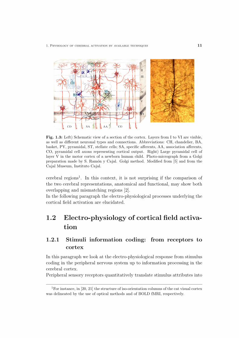
Fig. 1.3: Left) Schematic view of a section of the cortex. Layers from I to VI are visible,as well as different neuronal types and connections. Abbreviations: CH, chandelier, BA,basket, PY, pyramidal, ST, stellate cells; SA, specific afferents, AA, association afferents,CO, pyramidal cell axons representing cortical output. Right) Large pyramidal cell oflayer V in the motor cortex of a newborn human child. Photo-micrograph from a Golgipreparation made by S. Ramon y Cajal. Golgi method. Modified from [5] and from theCajal Museum, Instituto Cajal.
cerebral regions1. In this context, it is not surprising if the comparison of
the two cerebral representations, anatomical and functional, may show both
overlapping and mismatching regions [2].
In the following paragraph the electro-physiological processes underlying the
cortical field activation are elucidated.
1.2 Electro-physiology of cortical field activa-
tion
1.2.1 Stimuli information coding: from receptors to
cortex
In this paragraph we look at the electro-physiological response from stimulus
coding in the peripheral nervous system up to information processing in the
cerebral cortex.
Peripheral sensory receptors quantitatively translate stimulus attributes into
1For instance, in [20, 21] the structure of iso-orientation columns of the cat visual cortexwas delineated by the use of optical methods and of BOLD fMRI, respectively.
12 1.2 Electro-physiology of cortical field activation
a nervous code, through which information propagates along neuronal axons
to the central nervous system [3]. This neural code consists of the modula-
tion, inside axons, of the amplitude of sub-threshold2 synaptic potentials and
of the spiking rates3 (amplitude/frequency code) with changes in stimulus in-
tensity. Information coding also relies on the variation of the number of axons
involved (population code), depending on the stimulus extension. Finally, the
neural code is based on the change of the duration of sub-threshold potentials
and of spike trains (duration code), which depend concurrently on stimulus
duration and on the fiber characteristics (e.g. some receptors of peripheral
neurons respond only to stimulus transients). In each transmission step to-
wards the central nervous system, this code propagates mono-directionally
up to synaptic junctions, along the afferent axons involved; then, it trans-
lates in the number of total neurotransmitters Ntot released in the synaptic
cleft. As a consequence, Ntot is directly modulated by the three input factors
(frequency, population and duration) above mentioned. For instance, the
greater the concentration of neurotransmitters, the greater the amplitude of
graduated post-synaptic potentials above threshold values, which may give
rise to a greater frequency rate of generated post-synaptic action potentials
(e.g. depending on the involvement or not of inhibitory neurons)4.
For each neuron four distinct regions can be discriminated from a morpholog-
ical and functional point of view: its dendrites, its cellular body (or soma),
its axon and its pre-synaptic axon terminals. Starting with the arrival of an
action potential on the axon of an afferent neuron, it causes the depolariza-
tion of the pre-synaptic membrane of the axon terminal5, and, as a conse-
quence, the opening of voltage-dependent calcium (Ca2+) channels with the
entrance of Ca2+ in the intra-cellular space. This triggers exocytosis of the
pre-synaptic vesicles and release of neurotransmitters into the synaptic cleft,
which diffuse towards post-synaptic dendrite receptors (see Fig. 1.4, upper
right). Depending on the type of the synapse (excitatory/inhibitory)6 the
2Each neuron has a specific membrane potential threshold, above which action poten-tials are generated.
3Spiking rate is equal to the number of action potentials per unit time.4The information coding itself may not change, but the information is heavily mod-
ulated as it goes from peripheral to central nervous system, e.g. by the involvement ofinhibitory neurons.
5Depolarization means that the cross-membrane potential increases from the restingpotential VR (e.g. ∼ -60 mV) to higher values (between VR and +∞). On the contrary,the membrane is hyperpolarized if it potential is lower than VR.
6If a synapse is excitatory or inhibitory depends on what types of ion channels con-duct the post-synaptic current, which in turn is a function of the type of receptors and

1. Physiology of cerebral activation by available techniques 13
Fig. 1.4: Left) Draft of the functional organization of a neuronal cell. Upper right) En-larged view of synaptic processes triggered by the arrival of an action potential at thepre-synaptic terminals. Lower right) Excitatory post-synaptic potentials (EPSP) consti-tute under-threshold membrane changes. If the integrative processing of simultaneousEPSPs yields a super-threshold membrane potential, an action potential is generated (seeFig. 1.4, left and lower right). Modified from [3].
neurotransmitter interaction with receptors, in the post-synaptic membrane,
enables the trans-membrane crossing of sodium, potassium and chlorine ions
(Na+, K+, Cl−), leading to a post-synaptic membrane depolarization or hy-
perpolarization (excitatory/inhibitory post-synaptic potential, EPSP/IPSP).
As a consequence of a EPSP or IPSP on a post-synaptic membrane of a
cortical neuron, two currents will be generated, one flowing inside the neu-
ron down to the cell body (intracellular), and a matching return current, in
the opposite direction, through the extracellular path (conventionally called
direct)7, see Fig. 1.5. Because of the ohmic (resistive) feature of the extra-
neurotransmitters employed at the synapse.7For instance, due to the inflow of Na+ at an active site of a neuron (transmembraneous
current), the extra-cellular space around the depolarized dendrite will become charged
14 1.2 Electro-physiology of cortical field activation
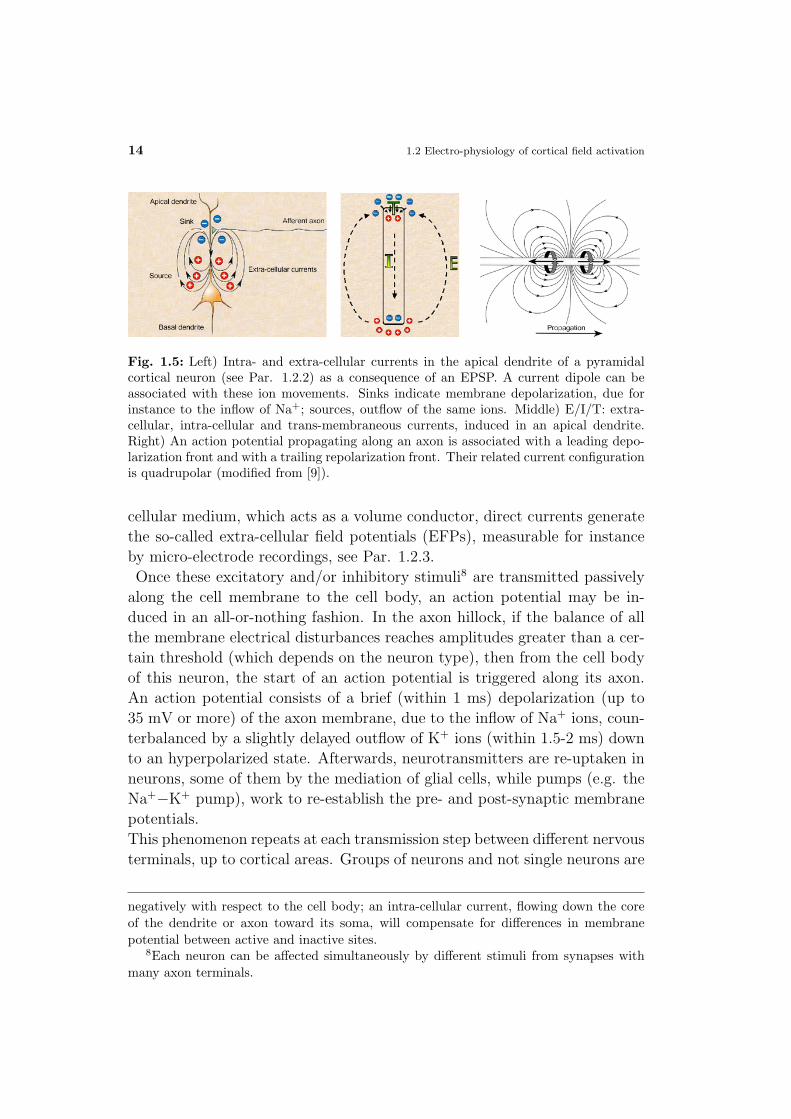
Fig. 1.5: Left) Intra- and extra-cellular currents in the apical dendrite of a pyramidalcortical neuron (see Par. 1.2.2) as a consequence of an EPSP. A current dipole can beassociated with these ion movements. Sinks indicate membrane depolarization, due forinstance to the inflow of Na+; sources, outflow of the same ions. Middle) E/I/T: extra-cellular, intra-cellular and trans-membraneous currents, induced in an apical dendrite.Right) An action potential propagating along an axon is associated with a leading depo-larization front and with a trailing repolarization front. Their related current configurationis quadrupolar (modified from [9]).
cellular medium, which acts as a volume conductor, direct currents generate
the so-called extra-cellular field potentials (EFPs), measurable for instance
by micro-electrode recordings, see Par. 1.2.3.
Once these excitatory and/or inhibitory stimuli8 are transmitted passively
along the cell membrane to the cell body, an action potential may be in-
duced in an all-or-nothing fashion. In the axon hillock, if the balance of all
the membrane electrical disturbances reaches amplitudes greater than a cer-
tain threshold (which depends on the neuron type), then from the cell body
of this neuron, the start of an action potential is triggered along its axon.
An action potential consists of a brief (within 1 ms) depolarization (up to
35 mV or more) of the axon membrane, due to the inflow of Na+ ions, coun-
terbalanced by a slightly delayed outflow of K+ ions (within 1.5-2 ms) down
to an hyperpolarized state. Afterwards, neurotransmitters are re-uptaken in
neurons, some of them by the mediation of glial cells, while pumps (e.g. the
Na+−K+ pump), work to re-establish the pre- and post-synaptic membrane
potentials.
This phenomenon repeats at each transmission step between different nervous
terminals, up to cortical areas. Groups of neurons and not single neurons are
negatively with respect to the cell body; an intra-cellular current, flowing down the coreof the dendrite or axon toward its soma, will compensate for differences in membranepotential between active and inactive sites.
8Each neuron can be affected simultaneously by different stimuli from synapses withmany axon terminals.

1. Physiology of cerebral activation by available techniques 15
usually involved and, at the cortical level, their functioning constitutes the
cortical field response.
1.2.2 Cortical input/output and intra-cortical process-
ing
How stimulus information is encoded and how it propagates up to cortical
areas was analyzed in the previous paragraph. We proceed then on evalu-
ating features of cortical neural activity; additionally, some aspects of the
morphometry which are of interest for several functional techniques are out-
lined.
The many aspects of neural activity, like pre- and post-synaptic excitation
and inhibition, sub-threshold depolarization and action potentials, can be
grouped at the cortical level in three distinct functional aspects: cortical
input, intra-cortical processing and cortical output [4]. While input and
intra-cortical processing consist mostly of sub-threshold integrative processes
and associative operations taking place for a given cortical field activation
(pre- and post-synaptic graduated potentials, comprising both excitatory and
inhibitory signals, but also intra-cortical spiking), output activity regards ex-
clusively spiking activity (propagation of action potentials).
This specific grouping of different functional processes is reflected by as many
anatomical distinct fiber connections. The neo-cortex receives all its infor-
mation (input) via the afferent fibers of pyramidal neurons9, which enter
the cortical layers, and sends its output through efferents of the same type of
neurons. Pyramidal cells are excitatory neurons; their axons, with regard to
afferents as well as efferents, reach sub-cortical structures (projectional neu-
rons or extrinsic connections, e.g. from the thalamus) or the cortex (intrinsic
connections), both in the other hemisphere (callosal or inter-cortical connec-
tions) or within the same hemisphere (intra-cortical afferents and efferents).
Afferent fibers terminate in specific layers, depending on which source they
come from (see Fig. 1.3); some of them terminate very precisely in specific
anatomical columns, as opposed to other afferents which have non-specific
terminations [2, 3]10. Similarly for the cortical output, each layer projects
9The name of pyramidal cells originates from the shape of their cellular bodies and,because of the plurality of their connections, are the major constituent of the cortex.
10For instance, most neo-cortical areas receive specific thalamic input primarily in layersIII and IV, while non-specific thalamo-cortical afferents are distributed diffusely over many

16 1.2 Electro-physiology of cortical field activation
its axons specifically to sub-cortical11 and other cortical areas.
Moreover, a great deal of processing is local (intra-cortical), reflecting the
intrinsic local circuitry of the cortex, which is mainly constituted of non-
pyramidal cells12 (e.g. chandelier, basket and stellate cells, see Fig. 1.3).
Non-pyramidal cells are primarily of inhibitory behaviour and have short ax-
ons which operate locally within the cortical layers. For this reason, they
are also called inter-neurons. However pyramidal cells play also a role for
intra-cortical processing, through their horizontal collateral ramification, as
well as the so-called U-fibers, which leave the cortex and re-enter it a few
centimeters away from the exit point.
In summary, information between brain areas (e.g. A and B) is communi-
cated via spike patterns carried by pyramidal neurons; these constitute the
above defined output for the region (for instance A), from which efferent
fibers carry out spike trains, and are excluded from the definition of input
for the region which receive this information (B). Conversely input and lo-
cal information processing (of region B, for instance) within a cortical field
primarily consists of sub-threshold integrative processing (respectively, pre-
and post-synaptic potentials of afferent fibers; as well as, for intra-cortical
processing, pre- and post-synaptic potentials of the local circuitry synapses)
but also includes the exchange of spike trains through local circuits.
The spiking output of coupled populations of neurons comprised in a corti-
cal field is determined by the non-linear dynamics of these populations. For
this reason the relationship between input and intra-cortical processing, on
one hand, and output activity may not necessarily be linear [7](interesting
comments also in [8]). For instance, when inhibitory neurons are involved, a
high local synaptic activity is not met by a concomitant spiking output.
Before elucidating the neural basis of intra-cortical and scalp potential recor-
dings (electrophysiological intra-cellular and EEG techniques, respectively)
and of scalp magnetic field recordings (MEG methodology), in this paragraph
we remark on a very crucial aspect of neuronal cells for the measurement
of neural activity by the same techniques. Beyond differences in laminar
placement and neurotransmitters used [2], the two classes of neuronal cells,
pyramidal and non-pyramidal, which constitute the cerebral cortex, have dif-
cortical areas, mainly in layer I and VI [4].11E.g. the cortico-thalamic connections project from layer V and VI.12Non-pyramidal cells have oval cell bodies and, morphologically, are heterogeneous,
with the majority of them being non-spiny, that is, without small spiny outgrowths ontheir dendrites. Non-spiny neurons are inhibitory, the remaining with varying behaviour.
1. Physiology of cerebral activation by available techniques 17
ferent morphology, and, in particular, different geometric organization inside
the cortical layers. Pyramidal neurons are oriented parallel to each other and
their apical dendrites cross over several cortical layers, perpendicular to the
cortex surface, while their collateral ramifications can stretch for some mm
in planes parallel to cortical layers. On the contrary, non-pyramidal neurons
do not have a preferred orientation with respect to the cortex surface, some
having dendrites in parallel planes, others in the orthogonal, still others in
planes at random angles with respect to the cortical layers, see Fig. 1.3.
The geometrical arrangement of cortical cells may also impact the outcome
of neuronal current detection by fMRI, as discussed in the present thesis, at
Par. 2.5.
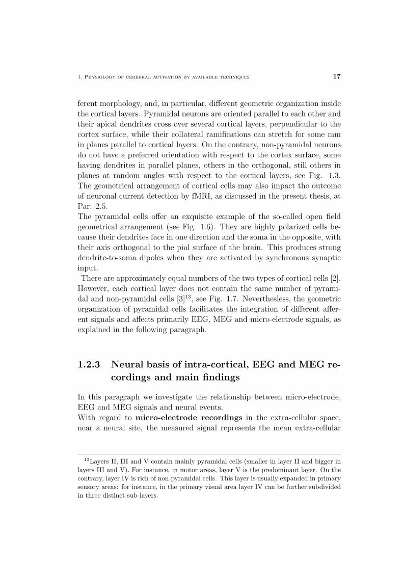
The pyramidal cells offer an exquisite example of the so-called open field
geometrical arrangement (see Fig. 1.6). They are highly polarized cells be-
cause their dendrites face in one direction and the soma in the opposite, with
their axis orthogonal to the pial surface of the brain. This produces strong
dendrite-to-soma dipoles when they are activated by synchronous synaptic
input.
There are approximately equal numbers of the two types of cortical cells [2].
However, each cortical layer does not contain the same number of pyrami-
dal and non-pyramidal cells [3]13, see Fig. 1.7. Neverthesless, the geometric
organization of pyramidal cells facilitates the integration of different affer-
ent signals and affects primarily EEG, MEG and micro-electrode signals, as
explained in the following paragraph.
1.2.3 Neural basis of intra-cortical, EEG and MEG re-
cordings and main findings
In this paragraph we investigate the relationship between micro-electrode,
EEG and MEG signals and neural events.
With regard to micro-electrode recordings in the extra-cellular space,
near a neural site, the measured signal represents the mean extra-cellular
13Layers II, III and V contain mainly pyramidal cells (smaller in layer II and bigger inlayers III and V). For instance, in motor areas, layer V is the predominant layer. On thecontrary, layer IV is rich of non-pyramidal cells. This layer is usually expanded in primarysensory areas: for instance, in the primary visual area layer IV can be further subdividedin three distinct sub-layers.
18 1.2 Electro-physiology of cortical field activation
Fig. 1.6: Example of closed (A, B), open (C) and open-closed (D) cell ensembles. “Closed”and “open” are referred to the electric and magnetic field variations produced in the extra-cellular space, outside of the dendritic extent of the cells (zero and non-zero, respectively).For instance, A and B represent cell ensembles from the oculomotor nucleus and superiorolive, respectively; C represents an array of pyramidal neurons from the accessory oliveand D a combination of the above arrangement. Also single cells (E, D) may fall into thesame categories (open/closed). Modified from [9].
field potential (mEFP14) from the weighted sum of all sinks and sources15
across multiple cells16. However, only a detailed anatomical and geometrical
information may ensure a correct interpretation of the mEFP signal. In-
deed, the superposition principle, which states that EFPs from multiple cells
add up linearly and algebraically throughout the volume conductor, implies
14See also Par. 1.2.1, for the definition of post-synaptic-potentials and of the inducedintra- and extra-cellular currents.
15For an extra-cellular intra-cortical micro-electrode recording, the inflow of Na+ at anactive site of a neuron, e.g. an apical dendrite of a pyramidal cell, appears as a currentsink (inward currents); from the same point of view, inactive membrane sites act as asource (outward currents) for the active regions.
16The weighting is attributable to the properties of lipid membranes of neurons, whichadd a great deal of capacitance to the volume conductor and endow it with low-pass filterproperties.
1. Physiology of cerebral activation by available techniques 19
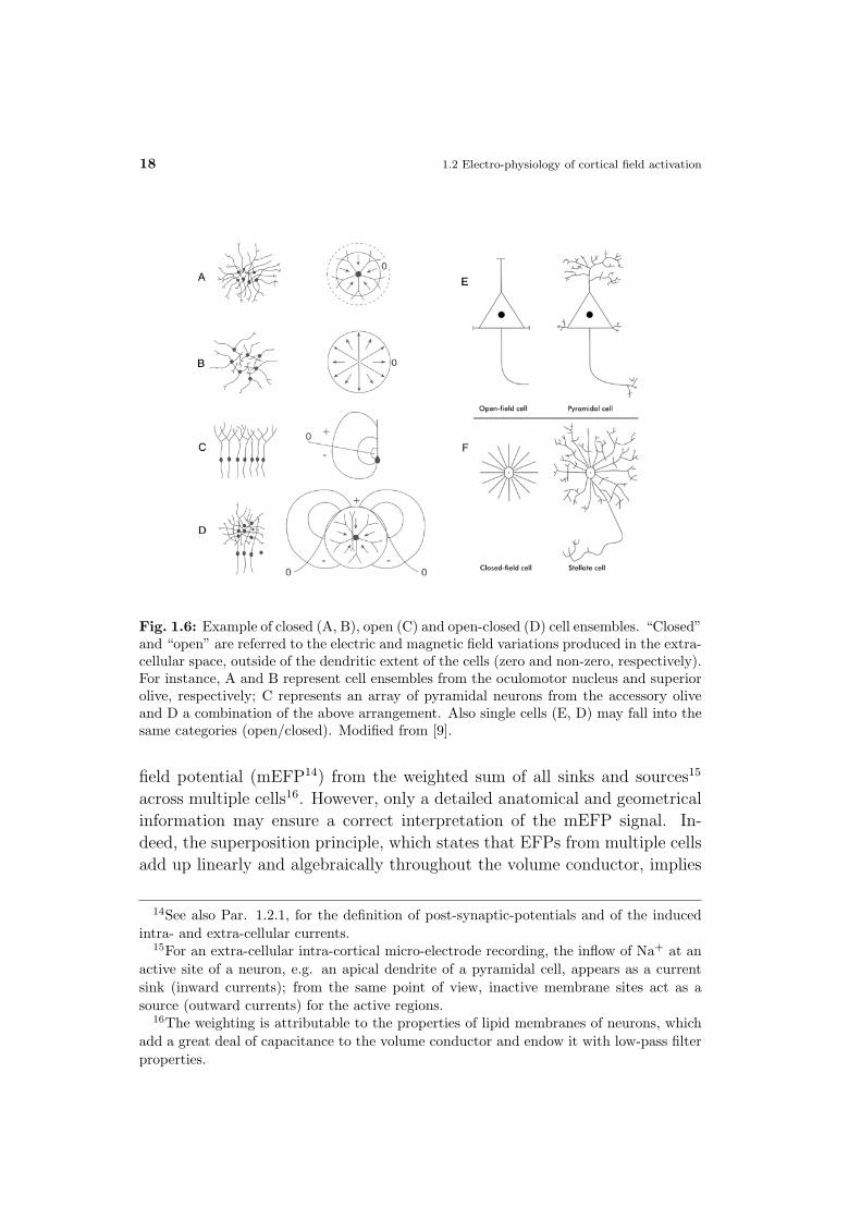
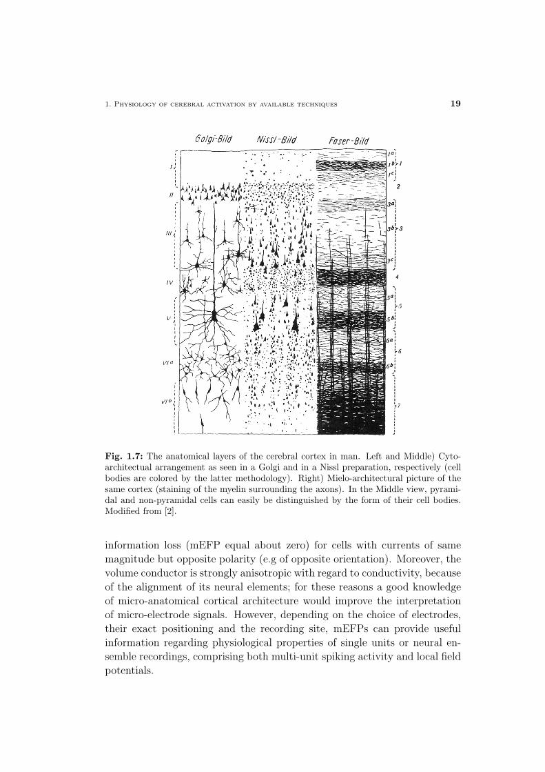
Fig. 1.7: The anatomical layers of the cerebral cortex in man. Left and Middle) Cyto-architectual arrangement as seen in a Golgi and in a Nissl preparation, respectively (cellbodies are colored by the latter methodology). Right) Mielo-architectural picture of thesame cortex (staining of the myelin surrounding the axons). In the Middle view, pyrami-dal and non-pyramidal cells can easily be distinguished by the form of their cell bodies.Modified from [2].
information loss (mEFP equal about zero) for cells with currents of same
magnitude but opposite polarity (e.g of opposite orientation). Moreover, the
volume conductor is strongly anisotropic with regard to conductivity, because
of the alignment of its neural elements; for these reasons a good knowledge
of micro-anatomical cortical architecture would improve the interpretation
of micro-electrode signals. However, depending on the choice of electrodes,
their exact positioning and the recording site, mEFPs can provide useful
information regarding physiological properties of single units or neural en-
semble recordings, comprising both multi-unit spiking activity and local field
potentials.

20 1.2 Electro-physiology of cortical field activation
If a micro-electrode with a small tip is placed close to the soma or axon
of a neuron, then the measured mEFP directly reports the spike traffic of
that neuron (single unit recording) and, frequently, that of its immedi-
ate neighbors as well17(spikes are discriminable from the termal noise of the
electrode tip for distances lower than ∼ 140µm).
When the impedance of the micro-electrode is sufficiently low and its exposed
tip is a bit further from the spike-generating sources, the electrode monitors
the totality of the potentials in the region (neural ensemble recordings).
The EFPs recorded under these conditions are related both to integrative
processes (dendritic events) and to spikes generated by several hundreds of
neurons [4, 5]. Traditionally, the two different signal types are segregated
by frequency band separation. A high-pass filter cut-off of ∼ 300-400 Hz is
used in most recording to obtain multiple-unit spiking activity (MUA);
a low-pass filter cut-off of ∼ 300 Hz is used to obtain the so-called local field
potentials (LFPs).
Data from a large number of experiments indicates that such a band sepa-
ration indeed underlies different neural events [4, 5]. MUA18, together with
single-unit recordings, which report only on the activity of few projection
neurons, is a measure of spiking activity, comprising both cortical output
and intra-cortical processing of the activated cortical field. LFPs, the low-
frequency range of the mEFPs signal, represent mostly slow cooperative ac-
tivity in neural populations, mainly synaptic processing19, and reflect the
17Single unit recording has the drawback of providing information on single receptivefields, with no access to subthreshold integrative processes; moreover it is biased towardcertain cell types and/or sizes (the greater the size, the simpler the micro-electrode detec-tion, with difficult recording of small neurons, e.g. inter-neurons).
18MUA, depending on the recording site and the electrode properties, most likely re-present a weighted sum of the extracellular action potential of all neurons within a sphereof ∼ 140 − 300 µm radius, with the electrode at its center. Spikes produced by thesynchronous firing of many cells can be enhanced, in principle, by summation and thusdetected over a larger distance.
19Until recently, local field potentials were thought to exclusively represent synapticevents. By combined field potential and intracellular recordings, it has been suggested thatthey instead reflect a weighted average of synchronized dendro-somatic components of thesynaptic signals of a neural population within 0.5-3 mm of the electrode tip. Later studiesprovided evidence of the existence of other types of slow activity unrelated to synapticevents, including voltage dependent membrane oscillations and spike after-potentials. Thelatter follow soma-dendritic spikes and are constituted of a brief delayed depolarization,the after-depolarization, and a longer lasting after-hyper-polarization. After-potentialshave a duration of tens of ms and most likely contribute to the generation of the LFPsignals, probably in the delta wave band (0-4 Hz).
1. Physiology of cerebral activation by available techniques 21
input of a given cortical area, as well as its local intra-cortical processing,
with the activity of excitatory and inhibitory inter-neurons included. LFPs
also mirror the extent and the morphology of dendrites in each recording
site and are not correlated with cell size. Hence, due to their geometrical
arrangement, pyramidal cells contribute maximally to LFPs.
For their specificity to the main cortical processes underlying brain function,
as well as for their elevated temporal and spatial resolutions, micro-electrode
recordings are an important tool for the neuro-physiologist; however, due to
their invasivity, they are mostly available for research on animals. For this
reason EEG and MEG approaches are attractive non-invasive solutions to
study human brain function: they are based on scalp measures of electro-
magnetic fields produced by electrical activity in a cortical field.
Instrumentation for EEG consists of a set of scalp electrodes coupled to high-
impedance amplifiers and of a digital data acquisition system [9, 10]. EEG
employs electrodes of a few mm to detect variation of the scalp electrical po-
tential, induced by neural activity, ranging from few to 100 µV; the smaller
the electrode in EEG recordings, the greater the sensitivity for small poten-
tial changes. With regard to MEG measurements [175, 179], superconductive
sensors (Superconducting QUantum Interference Devices, SQUIDs) housed
in a magnetically shielded room, are employed; they can detect magnetic
field variations, induced by cortical activity, as low as 50-900 fT.
Signal amplitudes in both measurements depend on the distance of the corti-
cal source from the measurement instrumentation, on the number of excited
neurons, on their synchrony and on their geometry.
For these reasons, it is widely believed [9, 10] that the primary source of EEG
and MEG signals are respectively extra- and intra-cellular20 current flowing
in apical dendrites of pyramidal cells in the cerebral cortex, caused by post-
synaptic potentials (PSPs). As also explained in the previous paragraph,
with regard to geometry, the pyramidal cells, with their apical surface run-
ning parallel to each other and perpendicular to the pial surface, form an ideal
open field arrangement and contribute maximally to both the macroscopi-
20EEG signals are produced by ohmic current flow in the head; for this reason theyare mainly affected by extra-cellular currents. However, EEG recordings are also highlysensitive to the conductivity of the brain, skull and extra-cranial tissue, which has to beaccounted for in the solution of the inverse problem (source identification). In contrast,MEG measures the magnetic field outside the head, induced by current flow within thebrain. In this case, the major contributor to the signal is the field induced directly byneural current generators, sometimes called the primary currents in contrast to secondaryor ohmic currents.
22 1.2 Electro-physiology of cortical field activation
cally measured EEG and the local field potential of scalp and intra-cellular
recordings, respectively. Conversely, neuronal structures in which dendrites
have random orientations generate closed fields, with electro-magnetic fields
hardly measurable outside its structure or close to it, see Fig. 1.6.
Conversely, action potentials, although having a greater amplitude than post-
synaptic potentials, contribute negligibly to scalp electro-magnetic recor-
dings. This can be explained considering their different field properties with
respect to graduated potentials and their lack of synchronization21.
Moreover, with regard to the geometry, inside an activated cortical field, due
to cerebral cortex folding, some pyramidal cells are oriented tangentially, oth-
ers radially and still others obliquely with respect to the scalp surface and
hence to the measurement electrode or sensor. For an exactly spherical scalp
surface, EEG(MEG) measurements detect primarily group of synchronous
currents of pyramidal cells oriented radially(tangentially)22 with respect to
the scalp, see Fig. 1.8. However, the use of a great number of electrodes (≥64), together with the fact that the actual scalp geometry is not precisely
spherical, enables also the detection of tangential(radial) sources as well.
The cortical activation field detected both by EEG and MEG signals is pro-
bably the average activity of 106 cortical neurons (50.000 or more in [11]).
The coherent activation of these large number of pyramidal cells in a small
area of cortex (some mm2, in plane) can be modeled as an equivalent current
dipole (ECD). ECDs are oriented normally to cortical surface because of its
columnar organization [12] and the solution of the inverse problem enables
the localization of ECDs, although with a linear spatial resolution of only 1
cm. For this reason EEG and MEG are considered imaging techniques, but
not in a strict sense. However, their optimal temporal resolutions (ms) has
proven and is still crucial for the investigation of fast cortical events.
More precisely, EEG, MEG and also intra-cortical recordings have allowed
the characterization of two basic types of neuro-electric activity: sponta-
neous brain activity and evoked responses. With regard to the first, as al-
ready demonstrated in the first EEG measurements of Hans Berger (1929)
21Indeed, the amplitude of the electro-magnetic field induced by an action potential, dueto its quadrupolar characteristic, decreases much more rapidly (r−3, r = distance from thesource) than that relative to post-synaptic potentials (dipoles and field decreasing as r−2);moreover, action potentials last for about 1 ms, and, in order to generate a signal detectableby EEG and MEG recordings, a great number of synchronous active neurons is required.Conversely, synaptic currents are long lasting (from 10 to 40 ms) and can add up efficientlyand give rise to detectable scalp signals, even without a perfect synchronization.
22This is also valid for their projection on a radial(tangential) direction only.

1. Physiology of cerebral activation by available techniques 23
Fig. 1.8: 1. Cells oriented pependicular (A) to the skull surface fail to generate an extra-cranial magnetic field detectable by MEG (see 2.), but produces electric potential changesmeasurable by EEG (panel 3.). The opposite for cells oriented parallel to the skull (C)which produce a significant radial(tangential) magnetic(electric) field. Cells denoted by Bhave intermediate features between cells A and C. Modified from [9].
in humans, brains “at rest” show an unexpected activity, characterized by
spontaneous low frequency signal modulations. Traditionally, these compo-
nents are classified in a number of specific frequency bands [13], known as
delta (δ, 0-4 Hz), theta (θ, 4-8 Hz), alpha (α, 8-12 Hz), beta (β, 12-24 Hz)
and gamma (γ, 24-40/80 Hz) bands, each with a distinct signal amplitude
(from 1 to 200 mV). These different rhytmic signal oscillations have been
associated with specific behavioral states (dreaming, relaxation, attention,
pathological conditions); however their function roles are still unknown.
Beyond background activity, responses to sensory-motor and cognitive events
related to different stimulus modalities [13] have been intensively studied by
both EEG and MEG, on one hand, and with micro-electrode recordings, on
the other, whenever possible. When a sensory stimulus is delivered, varia-
tions in EEG and MEG signals are called evoked potentials (EP) and evoked
24 1.3 The metabolic-hemodynamic response associated with cortical field activation
field (EF), respectively. More generally, event-related potentials or fields
(ERP and ERF) are EEG and MEG signal changes associated with an event
(sensory stimulus, motor act or endogenous event).
ERP/Fs result from a phase adjustment of cerebral rhythms with respect
to the event, in terms of a strict temporal relation of the response with the
stimulus, also called latency23. ERP/Fs yield increases of the signal power,
usually in the spectrum range from about 4 to 60 Hz. The amplitude of
ERP/Fs is at least an order of magnitude lower that that of spontaneous
activity (a few µV for ERPs): for this reason averaging the signals in phase
with the stimulus enable their extraction from the background signal.
Finally there is another class of responses, induced by a repetitive stimulus
(steady state potentials/fields, SSPs/SSFs). They consist of intense oscilla-
tions, but their latency is not always constant (if the oscillations are induced)
with respect to the stimulus [165]. They generally produce increases in the
average power, with no re-phasing of the signal.
1.3 The metabolic-hemodynamic response as-
sociated with cortical field activation
In the previous paragraph the different aspects of neuronal processes which
happen locally during brain activity were described: they are synaptic ex-
citation and inhibition, sub-threshold depolarization and action potentials
of the neuron soma; it was shown that they can also be grouped, on the
basis of specific features, into input, intra-cortical processing and output re-
sponses. The many different facets of brain activity may be not reflected
one to one by the metabolic or vascular response; rather all of them may
be translated into just one dimension of metabolism/blood flow according
to their consequent energy need. This point of view, linked to the concept
that the metabolic-vascular response is indirectly guided by neuronal events,
through their energy requests, has been recently challenged, see Par. 1.3.1.
Seminal efforts based on the combined use of different techniques, to discrim-
inate neuro-vascular coupling relative to each aspect of neural activity are
also promising in order to elucidate this issue (see Par. 1.4).
23ERP/Fs are constituted of wave-forms with positive and negative deflections (compo-nents). The sign depends on the position of the EEG electrode or of the MEG sensor withinthe superficial potential/field distribution, which depends on the cortical area activatedand on its orientation with respect to the scalp.
1. Physiology of cerebral activation by available techniques 25
However, whether or not the translation of electrical to the metabolic and he-
modynamic information embodies a loss of degrees of freedom, undoubtedly,
the complexity of the metabolic-vascular response and the great number of
actors involved is evident.
The brain requires energy to produce electric activity. Energy comes in the
form of oxygen and glucose, carried in the blood and provided to neurons
through the walls of capillaries [14]. Indeed the brain is a great energy con-
sumer: while it represents only 2% of the body weight in humans, this organ
accounts for approximately 25% of total body glucose utilization and almost
20% oxygen consumption of the whole organism. As has been recognized for
more than a century [15, 16], the brain’s information-processing capacity is
limited by the amount of energy available; so blood flow is increased to brain
areas where nerve cells are active.
The vaso-motor response occurs within seconds. However, exactly how the
flow is increased is uncertain: does energy demand or neural signaling regu-
late blood flow? The first subparagraph is dedicated to this issue.
Divergent opinions are expressed in the literature regarding whether locally
increased energy demands caused by electrical activity are accompanied by
oxidative or non-oxidative metabolic processes; also the role of glucose as the
main metabolic substrate has been challenged by several studies, with lactate
as the proposed alternative. In the second subparagraph we deal with these
issues, after a brief discussion on which and where are the greater energy
requests both at rest and during activation.
In the third subparagraph the recent models for the dynamics of oxygen
delivery, blood flow and blood volume are dealt with.
1.3.1 The neuro-vascular coupling: blood flow may be
controlled by energy demand or by neural sig-
naling
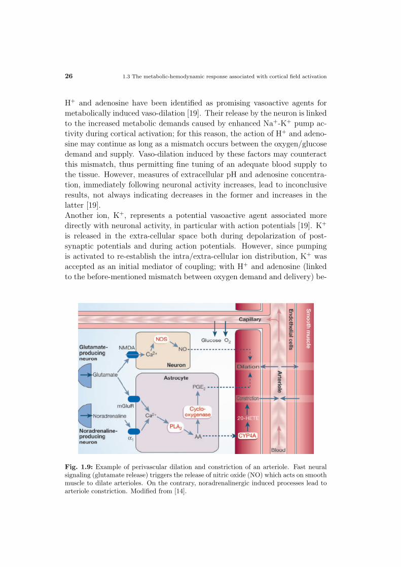
Flow in capillaries is controlled by the smooth muscle surrounding pre-
capillary arterioles. The smooth muscle constricts and dilates arterioles on
the basis of dedicated neural signaling (vasoactive agents) from the perivas-
cular side, as well as from the intravascular side. However, the former appear
to be the mechanism of major importance, see Fig. 1.9.
Two perivascular mechanisms may control blood flow [17]: the first is linked
to energy use; the second, discovered only recently, regards neural (neuro-
transmitter mediated) signaling to the local vasculature.
26 1.3 The metabolic-hemodynamic response associated with cortical field activation
H+ and adenosine have been identified as promising vasoactive agents for
metabolically induced vaso-dilation [19]. Their release by the neuron is linked
to the increased metabolic demands caused by enhanced Na+-K+ pump ac-
tivity during cortical activation; for this reason, the action of H+ and adeno-
sine may continue as long as a mismatch occurs between the oxygen/glucose
demand and supply. Vaso-dilation induced by these factors may counteract
this mismatch, thus permitting fine tuning of an adequate blood supply to
the tissue. However, measures of extracellular pH and adenosine concentra-
tion, immediately following neuronal activity increases, lead to inconclusive
results, not always indicating decreases in the former and increases in the
latter [19].
Another ion, K+, represents a potential vasoactive agent associated more
directly with neuronal activity, in particular with action potentials [19]. K+
is released in the extra-cellular space both during depolarization of post-
synaptic potentials and during action potentials. However, since pumping
is activated to re-establish the intra/extra-cellular ion distribution, K+ was
accepted as an initial mediator of coupling; with H+ and adenosine (linked
to the before-mentioned mismatch between oxygen demand and delivery) be-
Fig. 1.9: Example of perivascular dilation and constriction of an arteriole. Fast neuralsignaling (glutamate release) triggers the release of nitric oxide (NO) which acts on smoothmuscle to dilate arterioles. On the contrary, noradrenalinergic induced processes lead toarteriole constriction. Modified from [14].

1. Physiology of cerebral activation by available techniques 27
coming effective after a time lag, primarily in those situations in which the
K+ mechanism is not sufficient to yield an adequate O2 supply.
In addition, recent findings have shown that computationally active neurons
increase local blood flow by faster mechanisms. In the cerebellum, hippocam-
pus and neo-cortex, there is increasing evidence that blood flow is controlled
locally by fast neurotransmitters, e.g. glutamate and, perhaps, GABA [17].
These data suggest that the glutamate released by active neurons raises the
intra-cellular concentration of Ca2+ ions in post-synaptic neurons, thereby
activating the enzyme nitric oxide (NO) synthase, leading to the release of
NO, together with adenosine and arachidonic acid metabolites. These, in
turn, dilate pial arteriole and/or pre-capillary micro-vessels. In hippocam-
pus and neo-cortex only, exogenous GABA was able to dilate pre-capillary
micro-vessels.
Finally, it is known that dedicated intrinsic neural networks [17, 19] exert a
more wide-spread regulation of blood flow than the spatially restricted control
of fast transmitters. For instance, this global control of blood flow is provided
by dopaminergic, noradrenalinergic, serotoninergic and cholinergic fibers of
neurons innervating microvessels and producing mainly vaso-constriction of
the same (some of them also with the mediation of astrocytes).
Experimental evidence of a coarse control of CBF came first from observa-
tions with optical methods by Malonek and Grinvald [20]; their results may
indicate that vascular signals (flow) are distributed over a wider region than
that relative to the metabolic response. In a metaphor, the phenomenon was
described as of “watering the garden for the sake of one thirsty flower”24.
Concurrent with flow changes, are also blood volume changes. As the resis-
tance of the arterioles decreases, together with the relaxation of the smooth
muscle in their walls, the pressure drop across these vessels also decreases,
raising the pressure in capillaries and veins (flow in). The vessels may also
expand, due to the increased pressure, further increasing the cerebral blood
volume (CBV) [22]. Experimental studies by Grubb et al. [23] indicated that
the steady state relationship between CBF and CBV can be described with
a power law:
(1.1) CBV = CBFα;
24It was also confirmed by subsequent BOLD fMRI studies [21], where an increase oflocalization of the activation between the fast response (dip) and the later (flow related)positive BOLD response was found (see Par. 1.3.3 for a description of the BOLD responsephases).
28 1.3 The metabolic-hemodynamic response associated with cortical field activation
where the exponent α is approximately 0.4. However the law is strictly valid
only at steady state and experimental evidence is still needed to validate re-
cently proposed models for the pressure volume curve in dynamic conditions
[24, 25] (see also Par. 1.3.3).
Changes in blood volume may be compartmentalized. Indeed arteriolar di-
latation may be negligible, while the venous compartment may be more in-
volved in terms of volume changes. Finally with regard to capillaries, the
smallest vascular compartment, two hypothesis may explain flow regulation:
blood volume (capillary recruitment hypothesis25) may increase with the rise
in flow; however, a CBF enhancement may be driven by increases in blood
velocities as well.
1.3.2 Controversies regarding the locus of cerebral en-
ergy use and of the type of metabolism
Locus of cerebral energy use at rest
At rest, neurons consume an extremely high amount of energy, in the form
of Adenosine 5′-TriPhosphate (ATP), linked to their function [2, 18]. By
the use of classical biochemical methods26, ATP consumption at rest has
been divided between different metabolic mechanisms as follows: the Na+-
K+ ionic pump, which actively maintains the membrane potential at rest, is
the main consumer of ATP, of more than 65%; other pumps (Ca2+-H+, H+-
K+) together consume 1%; axoplasmic (or orthograde) and also retrograde
transport, from cell bodies to axon terminals and viceversa, of proteins, mem-
brane vesicles, organelles, seems to require a discrete sum of energy, at least
6% and anabolic processes (synthesis of neurotransmitters, proteins, glyco-
gen, lipids, nucleotides) consume another few %.
Locus of cerebral energy use during activation
During functional activation, each mechanism involved in neural signaling,
as well as in non-neuronal compartments (such as astrocytes), is enhanced.
A rise in the energy consumption is expected too: pre- and post-synaptic
25In this model capillaries are considered to have two functional states: inactive andactive. In the inactive state, blood cells do not pass, although plasma may, through thecapillary. Blood volume increases are accompanied by an increased fraction, p, of activecapillaries.
26In in vivo animals, drugs and inhibitors, selective specifically for one metabolic path-way, are delivered; on the basis of the oxygen or glucose need reduction, the energyconsumption for that specific pathway can be estimated.

1. Physiology of cerebral activation by available techniques 29
activity, both inhibitory and excitatory, and the propagation of action po-
tentials requires additional energy with respect to the resting condition.
The ATP consumption of the Na+-K+ ionic pump increases (around 52%),
[26–28] due to the reverse or modified trans-membrane ionic gradients asso-
ciated with both synaptic activity and the generation of action potentials.
Neurotransmitter re-cycling, in part mediated by astrocytes, contributes also
to the increased energy need (3%, [18]). Anabolic mechanisms not strictly
linked with neuronal activity, as well as axonal transport are expected to be
unchanged or transiently decreased, as opposed to all catabolic processes.
Autoradiographic studies at the cellular level in rats [27], initially showed
that most up-take of glucose occurred in the neuropil and not in the cell
bodies or in the glial cells. Creutzfeld [29] suggested that only 0.3-3% of
the energy used in cat and human brains is needed to support action poten-
tials. Hence it seemed that synaptic activity, rather than action potentials,
is associated with the local changes in energy consumption. A number of
studies [30] have concluded that it is mainly pre-synaptic, both excitatory
and inhibitory, rather than post-synaptic activity which induces increases in
glucose utilization. However, renewed theoretical calculations suggest that
the high signaling costs in the primate cortex are dominated by post-synaptic
currents (75%) and, in lower contributions (10%), by action potentials, with
pre-synaptic costs of only 7% [18], see Fig. 1.10.
With regard to the energy used by inhibitory signaling, it has been shown
that this mechanism, as for excitatory signaling, increases deoxy-glucose up-
take in the auditory system, during acoustic stimulation [31], although recent
controversial results have been found for blood flow and BOLD activity du-
ring inhibition [32, 33]27. Qualitatively many of the processes in both types of
neurons are identical (variation of membrane potential by ion fluxes) and en-
ergy expenditure increases for both. However, some considerations28 suggest
that inhibitory energy cost should be inferior to that of excitatory synapses.
27The first study [32] showed, by the use of optical methods and intra-cortical recordings,that flow increased locally when spiking activity was inhibited. In the second work [33],the authors did not find any change in the BOLD signal associated to inhibited regions;see also Par. 1.4.
28Inhibitory synapses are present in one tenth of the density, with compared to theirexcitatory counterparts in the cortex; furthermore, the electro-chemical gradient downwhich Cl− moves post-synaptically at inhibitory synapses is not as steep as that downNa+ moves at excitatory synapses, with less energy required to pump the ions back;finally less action potentials are generated in post-synaptic membranes when inhibitiontakes place (see in [17]).

30 1.3 The metabolic-hemodynamic response associated with cortical field activation
Oxidative metabolism of glucose fulfills cerebral energy requests
at rest
Several in vivo studies at the organ level have unequivocally determined that,
in normal physiological conditions, glucose is the obligatory energy substrate
for the brain at rest, where it is mainly oxidized to CO2 and water, with the
production of ATP, the energy unit [34, 35].
ATP is hence produced mainly oxidatively at rest, via the different ATP
Fig. 1.10: Sketch of an excitatory neuron and of a glial cell. Predictions of grey mattersignaling energy for rodents (first value) and primates (second value), relative to differentsub-cellular processes. Modified from [17].

1. Physiology of cerebral activation by available techniques 31
regulating mechanisms29. Indeed PET measurements30 with steady-state in-
halation of 15O and 2-(18F)fluoro-2-deoxyglucose (15O-PET and FDG-PET,
respectively) both in rats [36] and humans [37] indicate a ratio between cere-
bral oxygen consumption (CMRO2) and cerebral glucose utilization (CMRGlc)
around 5 in gray matter31. Given a stoichiometry of 6:1 mol of oxygen con-
sumed/mol of glucose through the oxidative pathway, these results indeed
indicate that at rest brain glucose is mostly oxidized and that only about 10
% of glucose follows other metabolic fates (non oxidative, as the anaerobic
glycolysis or protein, lipids, glycogen synthesis, as well as proteic precursor
of neurotransmitters).
Controversy about the type of metabolism and substrate em-
ployed during cerebral activation
The issue of the neuronal metabolism during cerebral cortex activation was
raised by the observations of Fox et al., again obtained by PET [38, 39]. They
observed a focal mismatch between variations of CMRO2 (5%), CMRGlc (30-
50%) and CBF (30-50%) during neuronal activity produced by prolonged
stimulation. Molar CMRO2/CMRGlc ratio for the increases of 0.4:1 were re-
ported. On the basis of these findings, the authors claimed that regulation of
29They are: glycolysis, that converts intra-cellular glucose to pyruvate, with a net pro-duction of 2 ATPs per glucose molecule (under anaerobic conditions pyruvate is convertedto lactate; however a net lactate production in aerobic conditions may take place, whenoxygen consumption does not match glucose utilization); the mitochondrial respirationthat consumes intra-cellular oxygen and pyruvate via the tricarboxylic acid cycle (TCA)and converts it in ATP and CO2, with a nominal balance of 36 ATP/glucose (oxida-tive metabolism); the buffering effect of phospho-creatine (PCr) that reacts with ADP torelease ATP and creatine (Cr).
30Positron Emission Tomography, PET, imaging is based on the production and detec-tion of paired 511 KeV annihilation photons (due to the annihilation of electron/positronpairs). This is achieved by the use of scintillators, sometimes with collimators, whichreject events that don’t occur simultaneously (within few ns). From the measurement ofthe accumulated radioactivity in various directions an image can be calculated by the socalled back-projection reconstruction method: the spatial distribution of the radioactivityis thus shown. Several positron emitting radio-isotopes are used: 15O is used for the mea-surement of cerebral blood flow (it is prepared as H15
2 O-labeled water); 18F (fluorine), asfluorodeoxyglucose, FDG, is an excellent agent for studying glucose metabolism. Duringactivation, enhanced annihilation photons production occurs, due to the local increasedoxygen and glucose consumptions [9].
31CMRO2 was found to be around 160 µmol/100 g brain weight/min and CMRGlc
around 30 µmol/100 g brain weight/min. Cerebral blood flow at rest (approximately 57µmol/100 g brain weight/min) was measured in normal adults by PET, too.
32 1.3 The metabolic-hemodynamic response associated with cortical field activation
blood flow is for purposes (i.e. anaerobic metabolism) other than oxidative
metabolism, which is already saturated at rest; as a consequence, the brain
acutely would consume much less energy than previously believed.
Experimental evidence in line with these results (∆CMRGlc >> ∆CMRO2)
came soon from works using PET [40, 41] and the Kety-Schmidt [42] tech-
niques; however, the amount of mismatch between glucose and oxygen con-
sumed varied considerably among investigations. The marked experimental
complexity, the low SNR and the adoption of several simplifying assumptions
may have affected the consistency of these results obtained by PET measure-
ments.
Decreases of cerebral glucose, without a concomitant estimation of CMRO2 ,
were also observed in proton Magnetic Resonance Spectroscopy (1H-MRS)32
studies [43–45]; since variations of CMRGlc were estimated from glucose con-
tent changes, results for glucose consumption were strictly related to the
adopted kinetics33. The hypothesis of a “transient” anaerobic glycolysis,
invoked to fulfill increased energy demands during sensory stimulation, was
further supported by means of proton Magnetic Resonance Spectroscopy (1H-
MRS) studies, optimized for lactate detection. Cerebral lactate variations
were investigated during prolonged brain activation [47–49]: these authors
reported increased lactate concentrations, with maximum lactate increases
in the first minutes of stimulation. However, their temporal resolution was
low (minutes), due to the poor SNR obtained for 1H-MRS of lactate: in-
deed, a great number of averaged spectra over time were needed in order to
observe a peak of lactate, whose concentration is already small (less than 1
mM) for brain at rest. On the contrary, Merboldt et al. [50] did not observe
any significant lactate variation for a wide range of experimental parame-
ters. However subsequent work [44, 45] by the same group furnished results
in contrast with this finding. Indeed in [44, 45], Frahm et al. refined the
technique and, with the use of sliding window averaging, reached a nominal
temporal resolution of 30 s, with a stimulation lasting for a few minutes.
Beyond lactate concentration, they concurrently measured glucose content,
321H-MRS measurement are based on the response of water and of several brain metabo-lites; after excitation, their return to the equilibrium state is detected: from relaxationtimes, amplitudes and positions of signal frequency peaks, each proton pertaining to acertain metabolite can be characterized, in terms of its concentration and of the chemico-physical properties of its environment.
33In the cited studies, the Michaelis-Menten equation was employed, which describesthe rate of substrate consumption with respect to its concentration, in steady-state kineticconditions.

1. Physiology of cerebral activation by available techniques 33
Fig. 1.11: Time-course of regional brain glucose (a), lactate (b) concentration,oxygenation-sensitive (c) and flow-sensitive (d) signal in the human primary visual cortexduring a 12 min protocol comprising 6 minutes of visual stimulation. Modified from [45].
cerebral blood oxygenation and flow, see Fig. 1.11. While lactate increased
only during the first minutes of stimulation with a peak at 2.5 min after task
onset, glucose consumption and increased flow were present throughout the
entire stimulation; the activated cortex was also hyper- and hypo-oxygenated
at the beginning and at the end of the stimulation, respectively. The authors
interpreted the result in the context of a switch of the metabolism from
anaerobic to aerobic34.
The main critical point of all mentioned studies, starting from Fox et al.’s
works to later lactate 1H-MRS investigations, is the adoption of prolonged
stimulations (up to tens of minutes): on one hand, they can produce com-
plex and uncontrolled adaptive phenomena; on the other, they are stressful
for subjects, whose cerebral responses are not really representative of typical
34Initially, according to the authors, anaerobic glycolisis, coupled by fast flow changesand transient hyper-oxygenation, could take place; then, during the steady state, thehemodynamic and metabolic parameters would recouple; finally the undershoot of thecerebral blood oxygenation would compensate for the initial anaerobic phase.

34 1.3 The metabolic-hemodynamic response associated with cortical field activation
Fig. 1.12: The ANLS model, proposed by Magistretti and Pellerin, for coupling of sy-naptic activity with glucose utilization. Astrocytes convey lactate to neurons to fulfill totheir energy requests, concurrently with the reuptake of neurotransmitters (glutamate-glutamine cycle). In particular glutamate would stimulate astrocytic glycolysis, which inturn produces lactate; this metabolite would than diffuse into the extra-cellular space, beabsorbed by neurons and finally be oxydized. Modified from [51].
physiological functional activations. A second question is the poor temporal
resolution achieved in these investigations, except for the improvement in
Frahm’s studies; it was sufficient to characterize steady-state conditions, but
much too low to investigate dynamic metabolic changes of functional activa-
tions.
During the years in which the above lactate measurements were performed,
Magistretti and Pellerin proposed a model for lactate, instead of glucose,
as the main substrate for neurons during activity (astrocyte-neuron lactate
shuttle, ANLS) [51], on the basis of a great number of experimental results
obtained in vitro [52–55], see Fig. 1.12.
An interpretation of some spectroscopic MR work [44] in the context of the
ANLS model were provided; however, the lactate increases (over minutes)
observed by 1H-MRS followed temporal dynamics too slow to account for
rapid cellular events (lactate production and transport from astrocytes to
neurons), faster than the regional vascular response.
The pivotal role in neuronal metabolism of astrocytic lactate of the ANLS
has been challenged by other findings [56–61]. For instance, by means of

1. Physiology of cerebral activation by available techniques 35
Fig. 1.13: A) Examples of the 1H-NMR spectra obtained from the same subject in corre-spondence of rest and of several acquisition delays (0 s, 3 s, 5 s, 8 s and 12 s) with respect tostimulus presentation onset (1 s duration). Repetition Time (TR) = 7.5-15 s (dependingon the acquisition delay used), Echo Time (TE) = 270 ms, 128 scans. The lactate peakis marked by an arrow. B) Inter-subject lactate time-course (percentage variations withrespect to the basal level of each individual), after the presentation of the same stimulusas in A). The data reported are mean ± s.d. values. The points which are significantlydifferent from the basal level are indicated with an asterisk (t-test with p < 0.01). Drawnfrom [60].
1H-MRS, Mangia et al. [60] found lactate decreases (minimum content at
5 s) and a subsequent return to baseline (at 12 s) after the beginning of a
brief stimulation (1 s duration), which indicated mostly a fast local lactate
consumption rather then an astrocytic production, see Fig. 1.13. The con-
sistent gain in temporal resolution, with respect to previous NMR studies,
was obtained by adopting a time-locked acquisition modality in the context
of an event-related experimental design.
A more traditional picture of cerebral energetics, where glucose is the main
neuronal substrate, as suggested by [62, 63], may explain more experimen-
tal evidence, without neglecting the important support of astrocytes for the
glutamate-glutamine cycle. Recently, Aubert and Costalat [26] have pro-
posed the use of comprehensive models of both the metabolic and vascular
responses to validate experimental findings, such as the lactate increase re-
ported in [44, 45]35; the importance of this approach relies on the fact that
35Interestingly the model which best reproduced Frahm’s data was based on an increasein oxygen consumption, regulated by intra-cellular oxygen and pyruvate concentrations

36 1.3 The metabolic-hemodynamic response associated with cortical field activation
it furnishes means by which to test hypothesis.
In conclusion, a definitive picture regarding the locus of energy use, the
type of metabolism and of substrate during cerebral activation still has to be
drawn, with the need for further experimental evidence, preferably in vivo
on humans [46].
1.3.3 The dynamics of oxygen delivery, blood flow and
blood volume: the physiological model for the
BOLD effect and other findings
In this paragraph, we deal with the issue relative to the dynamics of the
neurovascular response, mostly in terms of blood flow and volume increases,
needed to support energetic demands. This question concerns the underly-
ing physiological changes accompanying neuronal activation; however, in the
literature interest has recently shifted to explain the findings obtained by
neuro-imaging techniques, mostly those regarding fMRI.
Fox et al. [38, 39] reported for the first time a discrepancy between the large
increase in CBF and the relatively, if any, small increase in oxygen consum-
ption induced by prolonged stimulation. PET studies [40, 64, 65], together
with the work of Madsen et al. [42] using the Kety-Schmidt method con-
firmed this mismatch, with the exception of two studies performed by PET
[66, 67].
As a direct consequence of this finding, a local rise in blood oxygenation
should occur. Indeed, at steady state, the oxygen extraction fraction (E) is
linked to CMRO2 and CBF by Fick’s law [22, 68], which describes conserva-
tion of rate of oxygen delivery and oxygen uptake36:
(1.2) E = C−1O2a
CMRO2
CBF
and by the intra-cellular ATP/ADP ratio (also the involvement of a second messengergave good results). Their tests discarded the hypotheses of a total, as well as of an onlyinitial anaerobic metabolism.
36Fick’s law states that oxygen delivery is proportional both to blood flow and to thearteriovenous oxygen difference, CMRO2 = (CO2a−CO2c)CBF ; CO2a is the arterial oxygenconcentration and CO2c is the oxygen concentration at the end of the capillaries. Dividingboth sides of this relation by CO2a and considering the oxygen extraction fraction E =(CO2a − CO2c)/CO2a , Eq. 1.2 can be obtained.
1. Physiology of cerebral activation by available techniques 37
with Ca equal to the arterial oxygen concentration. An increase in CBF ex-
ceeding that of CMRO2 leads to decreased oxygen extraction and hence local
blood hyper-oxygenation.
The development of optical methods, in particular of non-invasive near-
infrared spectroscopy, NIRS [69]37, and of endogenous magnetic resonance
approaches (BOLD fMRI) [126–128] to investigate in vivo brain function,
has provided further experimental evidence and new insight. Given their
good temporal resolution of seconds or less, it was at last possible to aban-
don steady state-conditions and to study dynamic blood oxygenation changes
relative to brief stimulations of few seconds.
Optical measurements and interpretations
An oxy-hemoglobin (HbO2) rise, peaking several seconds after stimulation
onset, was observed by Malonek and Grinvald [20, 70] (see Fig. 1.14b), by
the analysis of in vivo intrinsic optical signals from cat cortex, and on hu-
mans in several NIRS studies [71–74].
Hence, the oxygenation rise expected from PET studies was confirmed also
in dynamic conditions. A total deoxy-hemoglobin (dHb) content decrease,
concomitant with the total HbO2 rise, was also observed (see Fig. 1.14a),
indicating that blood flow changes in capillaries in the activation phase are
mainly achieved by blood velocity changes, rather than of blood volume
changes38.
37Optical methods detect changes in the intrinsic or extrinsic optical properties of cere-bral tissue associated with brain activity [69]. By means of an optical apparatus, consistingof a light source and a light detector, the following intrinsic parameters can, for instance,be measured on the exposed brain tissue of animals: with respect to light absorption, theconcentrations of oxy-hemoglobin, deoxy-hemoglobin (indicators of blood oxygenation)and total hemoglobin content (linked to blood volume; with respect to the doppler shift(which gives the name to the Laser Doppler flowmetry technique), the blood cell velocity(and hence blood flow); with respect to light scattering, the membrane potential and cellswelling (markers for ion membrane exchanges, e.g. of action potentials); by means of flu-orescence phenomena, the NADH and flavoprotein content (indicators of the intracellularenergy status). With the recent application of near-infrared light, which penetrates bio-logical tissues reasonably well, it has become possible to investigate human brain functionthrough the intact skull. By means of NIRS, mostly absorption and scattering measuresare possible (no significant intrinsic fluorescence can be detected transcranially). Thetemporal resolution of optical and NIRS methods is in the ms range; however, despite ofthe use of multi-detector arrays, e.g. in NIRS, they lack in spatial resolution and depthpenetration. In addition, reconstruction of the optical path length is non-trivial and isbased on several assumptions.
38A dissociation of blood flow and oxygen consumption do indeed imply that HbO2 mustrise, see Eq. 1.2; however, not necessarily, it implies a drop in capillary dHb. If the flow

38 1.3 The metabolic-hemodynamic response associated with cortical field activation
Fig. 1.14: Time-course of dHb, a) and of HbO2 , b), following a 4 s stimulation (in shadow)measured by optical imaging spectroscopy in the cat cortex (modified from [20]).
Finally, at the very early stages of stimulation (1-2 s) an unexpected dHb
rise, previous to the drop, was observed [20, 75] (see Fig. 1.14a), which was
interpreted as an increase in oxygen extraction before the flow increases39.
Findings about increase in dHb were challenged by subsequent optical mea-
sures on rat cortex [77], where it was not revealed; the authors explained
their result by showing that an incorrect analysis of the optical path length
could lead to an artifactual initial increase. Nonetheless, Jones [78], further
added the controversy by obtaining an initial dHb increase, using the same
sophisticated path length analysis of Lindauer.
BOLD experimental evidence and interpretations
Since its inception [126–128], the application of BOLD fMRI to study human
brain function has furnished results in support of the findings via optical
methods. The cornerstone of blood oxygenation level-dependent (BOLD)
fMRI (ref Hoogenraad01) is the change of the total dHb content of venous
increases are driven by blood volume increases (capillary recruitment hypothesis), thencapillary dHb content can remain constant, despite the above-mentioned dissociation. Ifthere is an increase in blood velocity (blood volume constant), dHb can drop. This becausetotal HbO2 and dHb contents (respectively proportional to E·CBV and to (1-E)·CBV) areaffected by both changes in the oxygen extraction fraction (E) and in blood volume changes(CBV) [30].
39Note that there was not a concurrent decrease in HbO2 ; so, as pointed out later byBuxton [76], the result supported more the idea of an interplay between volume and oxygendelivery, rather than oxygen delivery only, see below.

1. Physiology of cerebral activation by available techniques 39
Fig. 1.15: A) Measured hemodynamic response function averaged over 6 subjects, relativeto a visual stimulus flickering at 8 Hz (onset at the 11th scan, duration 3.6 s - modifiedfrom [83]). The tree-phasic behaviour of the hemodyanamic response is visible. B) Modelof the impulse-hemodynamic response function (i-HRF), assumed as a reference in theanalysis tool SPM2 for a 1 s stimulus duration. Usually, only the positive response andthe undershoot are used for data fit, since they account for the main signal variance. C)Spectral density power of the i-HRF. As visible, the i-HRF is mainly constituted of slowtime-varying components, with no power at frequencies greater than 0.2 Hz.
blood40, in order to respond to neuronal activation. The BOLD effect on the
MR signal regards both the extra-vascular and the intra-vascular compart-
ments, both static and diffusing water spins: for its complexity and impor-
tance for the current study we explain the BOLD bio-physical model at Par.
2.3. In brief, the BOLD signal is expected to decrease if dHb increases and
vice-versa.
Several experimental results obtained for the BOLD hemodynamic response
function (hrf) indicate a three-phasic behaviour, see Fig. 1.15:
• a rapid response in terms of a pre-undershoot (often called a “dip”)
within the first 2 s of activity observed at high fields by [79–82] and
also at 1.5 T [83], but not by Fransson et al. [84] nor by Silva et al.
[85], indicating a total dHb increase;
• a subsequent increase, starting and peaking, with respect to stimulation
onset, approximately after 2 s and 5-6 s ([86, 126]; then a plateau as
long as the stimulation continues; this overshoot indicates a total dHb
decrease;
• a final return to baseline with a post-stimulus undershoot lasting for
about 10-30 s, reported in [44, 87] and indicating a total dHb increase.
40The BOLD effect influences protons of both the intra- and extra-vascular compart-ments. However, while the extra-vascular signal depends on the total dHb content ∼(1-E)·CBV, the intra-vascular only on the dHb concentration ∼(1-E), according to the Bal-loon model (see in [24]).

40 1.3 The metabolic-hemodynamic response associated with cortical field activation
The physiological basis of these complex BOLD signal dynamics is not yet
fully understood; some aspects, primarily regarding the ’dip’, are still not
convincingly explained. The main reason relies on the dynamic interplay be-
tween variations in paramagnetic dHb and several physiological parameters
which change to fulfill increased metabolic demands of neurons in activ-
ity. They are cerebral blood flow (CBF), cerebral metabolic rate of oxygen
(CMRO2), and cerebral blood volume (CBV), a factor for long time underes-
timated in importance in determining BOLD responses. Still other factors,
and their governing dynamics, only recently outlined41 [22, 24, 26], may also
be determinant for the dHb content.
With regard to the second phase of this three-phasic behaviour, the BOLD
signal positive sign (dHb decrease) confirmed the decrease in the total dHb
content observed after some seconds with respect to stimulation onset by
optical techniques (see Par. 1.3.3 and Fig. 1.14a), and which was concomi-
tant with the total HbO2 rise. It was also an indicator (see Eq. 1.2) of
the over-compensatory flow response with respect to oxygen consumption
(CBFCMRO2) observed in PET studies for steady state activated condi-
tions ([38, 39], see at pag. 27). The first fMRI experimental evidence regar-
ding both CBF and CMRO2 on human cortex during activation came soon
and also supported these findings. Since CMRO2 is not directly measurable
by fMRI, it can be estimated by concurrent BOLD and CBF measurements;
CBV42 is calculated from CBF by the use of the Grubb’s law (Eq. 1.1)43 and
an analytical relationship linking CMRO2 with the three measured signals
(BOLD, CBF, CBV) is assumed. By the use of a calibrating procedure44
41For example, the venous viscoelastic properties, in the form of the time constant τV ,which affects the flow out in the venous side [22, 24], or the neuronal stimulation levelwhich modulates the venous oxygen concentration and hence E [26].
42Both CBF and CBV can be measured by perfusion fMRI techniques; however theneed for an exogenous contrast for the CBV measurement (bolus tracking) has limited itsapplication in vivo, as opposite to CBF measurements, performed in vivo by the use ofendogenous contrast (e.g. arterial spin labeling). However, a new perfusion MRI technique,promising for CBV measurements over time and based on an endogenous contrast, wasrecently proposed by Lu et al. [88].
43There is only one study which reported the measure of the three physiological param-eters, BOLD, CBF, CBV, on humans in vivo by three independent fMRI techniques [89].The authors suggested a great deal of caution when applying Grubb’s law.
44The most used method is to measure BOLD and flow changes in hypercapnic con-ditions. Hypercapnia is a physiological reference condition obtained by carbon dioxide(CO2) breathing. It is a poorly understood physiological phenomenon; however, it is wellestablished that it highly raises CBF and that, probably, has little or no effect on CMRO2 .
1. Physiology of cerebral activation by available techniques 41
for the baseline, a quantitative estimate of CMRO2 is hence possible, but
is performed with steady state assumptions. Following this strategy, several
authors [68, 90–93] showed via fMRI that the estimated oxygen consumption,
although not zero, is lower than changes in CBF, in agreement with previ-
ous PET results45. The peak in blood oxygenation during neural activity
was hence evidence reinforced by a great number of experiments and by the
use of several techniques. However, a pivotal question was still unexplained:
why should flow increase much more than the oxygen need? Buxton and
Frank [94] gave an interesting interpretation of the mismatch between flow
and oxygen metabolism changes during brain activation. In terms of their
oxygen limitation model, there was evidence of a tight coupling, rather than
uncoupling, of flow and metabolism. The oxygen limitation model was based
on the idea that oxygen delivery is limited at rest [95]. The model predicted
that disproportionately large changes in blood flow are required in order to
support small changes in the O2 metabolic rate46.
Later, Hyder. et al. [96] extended the oxygen limitation model including
a variable oxygen diffusivity proportional to blood flow; some years later,
Mayhew et al. [97] showed, by optical imaging spectroscopy and LDF47 on
The lack of a convincing demonstration of the latter claim does not point in favor of theuse of hypercapnia as a control reference; besides, the hemodynamic responses during neu-ronal activation and during hypercapnia should be similar for calibration purposes, butexperimental evidence for this is lacking.
45Hoge et al. [90] shows also that there is a simple graded relationship between CBFand oxygen metabolism in the human visual cortex during sustained visual stimulation,indicating a tight coupling between the two physiological changes.
46Two assumptions were made by the authors: first, all brain capillaries are perfusedat rest; hence capillary recruitment cannot take place and increases of flow are matchedby rises in blood velocities; second, all the oxygen which leaves capillaries is metabolized,with a null tissue oxygen concentration. In this condition, a decreased capillary transittime (due to increased blood velocity) leads to the drop in E, which has a functional role,rather than serving as a marker of uncoupling. Indeed the O2 diffusion gradient betweencapillaries and mithocondria drives the O2 flux from the first to the second compartment;in order to increase the net flux (and hence CMRO2), the gradient must be increased.This can only be achieved by raising the capillary pO2, by reduction of E (see [94]). This,considering Eq. 1.2, can be achieved if CMRO2 CBF.
47Laser Doppler flowmetry (LDF) is a well-established non-invasive technique for con-tinuous monitoring of cerebral blood flow (CBF). LDF has bridged the temporal gapbetween electro-physiology and vascular physiology. It has a time resolution in the msrange, while the in-plane spatial resolution is in the range of hundreds of µm. In depthresolution varies as a function of the wavelength of the laser beam and the separationdistances of the transmitting and recording optical fibers in the probe. LDF allows hencea laminar analysis of CBF relative to brain micro-circulation [32].

42 1.3 The metabolic-hemodynamic response associated with cortical field activation
Fig. 1.16: Possible time-courses of CBF and CMR02 , which may explain the early dip ofthe BOLD signal. Modified from [135]).
rats, that neither of the two models gave good account of their data; only
considering a non-null tissue oxygen concentration, moderated by changes
due to increased metabolic demands, a more convincing model (the Oxygen
Transport to Tissue, OTT, model) could be formulated48. Buxton [76] has
recently revised the oxygenation limitation model, by including a buffer of
available tissue oxygen, with the CBF regulation directly linked to maintain
the buffer at a constant level.
The interpretation of the BOLD positive response was hence furnished in
terms of a coupling of metabolism and flow. On the contrary, in terms of
the interplay of the physiological parameters CBF and CMRO2 , both the dip
and the post-undershoot seemed to indicate a metabolic/flow uncoupling.
With regard to the fast BOLD response, the “dip”, it could indicate a pos-
sible increase in oxygen extraction before flow increased (see Fig. 1.16). If
confirmed, it could add additional experimental evidence to the fast dHb rise
within the first 2 s observed by optical studies. The final undershoot was
also an unexpected phenomenon; it was interpreted, again, only in terms of
48The presence of O2 in the tissue could also be fundamental to explain the initial dipvariability; Mayhew et al. showed that hyper-oxygenation reduces or eliminates the initialdip; nevertheless Lindauer, [77], used a high concentration of inspired O2.

1. Physiology of cerebral activation by available techniques 43
CBF and CMRO2 , as an elevated oxygen extraction, after flow has returned
to baseline, required to replenish depleted tissue oxygen stores [98] or to com-
pensate for the initial anaerobic phase of activation [44, 87].
Buxton et al. [24] again provided an interesting explanation for the under-
shoot and also an alternative understanding for the dip. Motivated by the
observation in an animal study of Mandeville et al. [99] that CBV returned
to baseline more slowly than CBF after the end of the stimulus, Buxton et
al. hypothesized that the key parameter for explaining both the dip and the
undershoot could be CBV and its dynamics (time-constants) with respect
to flow changes. They formulated a model, the so-called Balloon model,
which was an extension of the oxygen limitation model. With the same
assumptions as the latter, they modeled the venous compartment49 as an
expandable balloon, due to increases in CBF. The amount of swelling of the
venous balloon is modulated by the bio-mechanical properties of the vessel
(pressure/volume curve), in terms of the difference between the driving force,
the flow in (Fin(t) or CBF), and the flow out (Fout), which is a function of
the venous volume Vv50. In this context changes in total dHb content (dHb),
measured by BOLD, are related to CBF, E and Vv, as well as to CO2a by the
following equation51:
(1.3)d(dHb)
dt= Fin(t)ECO2a − Fout(Vv)
dHb
Vv
.
By modeling and by experimental validation on humans through BOLD and
perfusion CBF measurements, the authors showed that the undershoot could
be caused by a return to baseline slower for blood volume than for blood
flow52. In addition, with regard to the dip, Buxton et al. [24] demonstrated
that a decrease in BOLD signal at the beginning of stimulation could be given
by a rapid increase in blood volume before the flow changes start. Buxton
criticized the interpretation that only changes in E (and hence of CBF and
CMRO2 , only) are responsible for the dip, as suggested in previous optical
studies [20]. In his opinion, the lack of a HbO2 decrease concurrent with the
49In their model, blood volume changes occur primarily in the venous compartment,since they assumed no capillary recruitment and negligible arteriolar dilation.
50Mandeville et al. [25] proposed a similar ’windkessel’ model, to embody the sameconcept and provide a biomechanical mechanism for a delayed CBV return to baseline.
51At steady steate Fout=Fin and dHb = ECO2aVv=CMRO2Vv
CBF .52If preliminary experimental validation of this dynamic model has been furnished,
however, its central premise (the slow CBV return to baseline) has not been yet definitelyestablished due to the difficulty of CBV measurements.
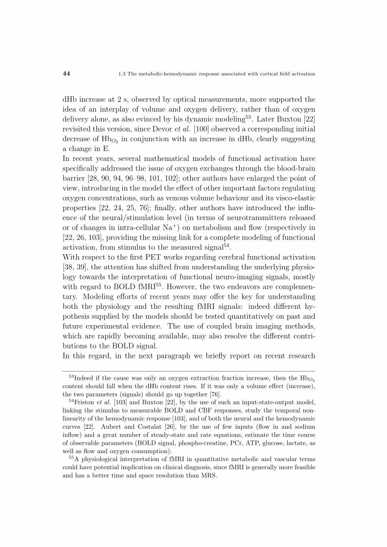
44 1.3 The metabolic-hemodynamic response associated with cortical field activation
dHb increase at 2 s, observed by optical measurements, more supported the
idea of an interplay of volume and oxygen delivery, rather than of oxygen
delivery alone, as also evinced by his dynamic modeling53. Later Buxton [22]
revisited this version, since Devor et al. [100] observed a corresponding initial
decrease of HbO2 in conjunction with an increase in dHb, clearly suggesting
a change in E.
In recent years, several mathematical models of functional activation have
specifically addressed the issue of oxygen exchanges through the blood-brain
barrier [28, 90, 94, 96–98, 101, 102]; other authors have enlarged the point of
view, introducing in the model the effect of other important factors regulating
oxygen concentrations, such as venous volume behaviour and its visco-elastic
properties [22, 24, 25, 76]; finally, other authors have introduced the influ-
ence of the neural/stimulation level (in terms of neurotransmitters released
or of changes in intra-cellular Na+) on metabolism and flow (respectively in
[22, 26, 103], providing the missing link for a complete modeling of functional
activation, from stimulus to the measured signal54.
With respect to the first PET works regarding cerebral functional activation
[38, 39], the attention has shifted from understanding the underlying physio-
logy towards the interpretation of functional neuro-imaging signals, mostly
with regard to BOLD fMRI55. However, the two endeavors are complemen-
tary. Modeling efforts of recent years may offer the key for understanding
both the physiology and the resulting fMRI signals: indeed different hy-
pothesis supplied by the models should be tested quantitatively on past and
future experimental evidence. The use of coupled brain imaging methods,
which are rapidly becoming available, may also resolve the different contri-
butions to the BOLD signal.
In this regard, in the next paragraph we briefly report on recent research
53Indeed if the cause was only an oxygen extraction fraction increase, then the HbO2
content should fall when the dHb content rises. If it was only a volume effect (increase),the two parameters (signals) should go up together [76].
54Friston et al. [103] and Buxton [22], by the use of such an input-state-output model,linking the stimulus to measurable BOLD and CBF responses, study the temporal non-linearity of the hemodynamic response [103], and of both the neural and the hemodynamiccurves [22]. Aubert and Costalat [26], by the use of few inputs (flow in and sodiuminflow) and a great number of steady-state and rate equations, estimate the time courseof observable parameters (BOLD signal, phospho-creatine, PCr, ATP, glucose, lactate, aswell as flow and oxygen consumption).
55A physiological interpretation of fMRI in quantitative metabolic and vascular termscould have potential implication on clinical diagnosis, since fMRI is generally more feasibleand has a better time and space resolution than MRS.
1. Physiology of cerebral activation by available techniques 45
regarding the coupling between the electro-physiological and metabolic re-
sponses, measured by combined techniques.
1.4 The neuro-vascular coupling and fMRI
signals may reflect synaptic rather than
spiking activity
Some open questions of cerebral physiology regard which feature of neuronal
activity is reflected by the metabolic-hemodynamic response (see also Pag.
25): synaptic activity, or action potentials? Moreover, do both excitatory and
inhibitory circuits evoke metabolic responses? These questions are also cru-
cial for both modeling and interpreting metabolic-vascular based signals (e.g.
those measured by fMRI approaches or optical methodologies). Interesting
answers to these issues came recently through the development of experimen-
tal approaches able to record simultaneously both the electro-physiological
(EEG, MEG and intra-cortical measurements) and the metabolic-vascular
cerebral responses (BOLD or perfusion fMRI, optical strategies), see for in-
stance [104–109] for the combination of EEG-fMRI.
Recent investigations, using different techniques, have suggested a linear rela-
tionship between neural activity and the subsequent hemodynamic response
in studies involving monkeys ([6, 110, 111] and rats [112–115]). Ten years or
more of brain mapping were saved! However, with regard to specific features
of neural activity the experimental results don’t agree.
Some of these studies show that the metabolic-hemodynamic response mir-
rors the generation of action potentials. Notably, Rees et al. [110] , compared
fMRI results on humans and electrophysiological (single-unit) measurements
in area V5 in monkeys. These authors suggested that the BOLD signal is
directly proportional to the average neuronal firing rate, with a constant of
proportionality of approximately 9 spikes/s and per percent BOLD increase.
The work of Heeger et al. [111] on area V1 in monkeys confirmed the lin-
ear relationship between the two measurements, although with a constant of
proportionality lower about 20-fold56.
Other work addressed synaptic, rather than spiking, activity relative to the
56These are pioneering works; however, results would be more robust if simultaneousintra-cortical and fMRI measurement on the same subject/animal would be performed.
46 1.4 The neuro-vascular coupling and fMRI signals may reflect synaptic rather than spiking activity
coupling with the metabolic-hemodynamic response. Among them, Lau-
ritzen, Mathiesen et al. [32, 112, 113] investigated the cerebellar cortex, by
measuring LFPs, single-unit activity and changes in cerebral flow by means
of LDF. These authors demonstrated that the spike rate in the principal
target cell of a brain region (i.e. the efferent cell) does not reflect vascu-
lar response amplitude. Indeed, both LFP and CBF increased at the same
time that spiking activity ceased. Instead, sub-threshold integrative synaptic
processes (especially post-synaptic, but with a possible contribution of pre-
synaptic elements as well) triggered changes in the local micro-circulation
and local metabolic consumption57.
Simultaneous fMRI and electro-physiological recordings on monkey brains,
performed by the group of Logothetis [6], also suggested that the BOLD con-
trast mechanism directly reflects the neural responses elicited by a stimulus,
more with regard to synaptic than to spiking activity. The hemodynamic
response correlated better with the LFPs (see Par. 1.2.3), rather than with
MUA measurements [4, 6]. Besides, the multi-unit response exhibited strong
adaptation (return to baseline at about 2.5 s after stimulus onset), while
LFP remained elevated for the entire duration of the stimulus, see Fig. 1.17.
On the basis of this finding, as well as for EEG and MEG recordings, the
authors inferred that the origin of BOLD signal probably relates more to
input and intra-cortical processing than to spiking activity. They suggested
also that their statement is only apparently in contrast with the work of
Rees et al. [110] and Heeger et al. [111]. Indeed, it is reasonable to ex-
pect that output activity will usually correlate with neurotransmitter release
and pre- and post-synaptic currents, when input into a particular area plays
what is primarily a modulatory role; however, functional experiments may
reveal activation in areas in which physiological experiments find no spiking
activity. An exquisite example of such a dissociation between intra-cortical
processing and output of a brain structure is indeed offered by Mathiesen et
al. [112, 113].
Although Loghotetis et al. found that LFPs correlated better to the BOLD
response, the relationship between LFPs, synaptic activity and input/intra-
cortical processing is not one-to-one (as evinced in Par. 1.2.2) and vice-
57These investigators stimulated the parallel fibers (PFs) of cerebellum, while recordingthe Purkinje cell (PC) activity. The PFs excite mono-synaptically the PC and inhibitdi-synaptically the same neuron, through the basket cells. The net effect of the PFs wasan inhibition of the spike activity of the PC, although at the same time synaptic activitycould have been increased.
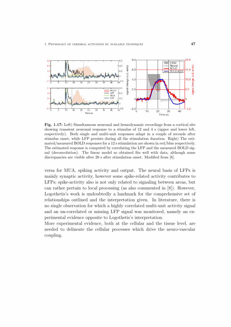
1. Physiology of cerebral activation by available techniques 47
Fig. 1.17: Left) Simultaneous neuronal and hemodynamic recordings from a cortical siteshowing transient neuronal response to a stimulus of 12 and 4 s (upper and lower left,respectively). Both single and multi-unit responses adapt in a couple of seconds afterstimulus onset, while LFP persists during all the stimulation duration. Right) The esti-mated/measured BOLD responses for a 12 s stimulation are shown in red/blue respectively.The estimated response is computed by correlating the LFP and the measured BOLD sig-nal (deconvolution). The linear model so obtained fits well with data, although somediscrepancies are visible after 20 s after stimulation onset. Modified from [6].
versa for MUA, spiking activity and output. The neural basis of LFPs is
mainly synaptic activity, however some spike-related activity contributes to
LFPs; spike-activity also is not only related to signaling between areas, but
can rather pertain to local processing (as also commented in [8]). However,
Logothetis’s work is undoubtedly a landmark for the comprehensive set of
relationships outlined and the interpretation given. In literature, there is
no single observation for which a highly correlated multi-unit activity signal
and an un-correlated or missing LFP signal was monitored, namely an ex-
perimental evidence opposite to Logothetis’s interpretation.
More experimental evidence, both at the cellular and the tissue level, are
needed to delineate the cellular processes which drive the neuro-vascular
coupling.

Chapter 2
Neuronal current fMRI,
proposal for an alternative
approach to BOLD fMRI
For its high spatial resolution and robustness, fMRI is one of the most pow-
erful imaging techniques for studying brain function. Among the various
current MR imaging methodologies, such as perfusion, primarily the BOLD
approach has been developed most and it is used routinely for functional
brain mapping. BOLD fMRI detects blood oxygenation changes associated
with neuronal activity and is limited in resolution by the temporal and spa-
tial scales of the hemodynamic response.
In this PhD thesis we discuss the feasibility of detecting functional changes
more directly linked to neuronal currents then the secondary hemodynamic
response by MRI: if the primary magnetic changes around cerebral electri-
cal sources were detectable via MRI a new functional approach, “neuronal
current fMRI”, would be available, and the study of in vivo human cerebral
physiology and brain mapping would significantly gain in specificity.
The effect of paramagnetic deoxyhemoglobin, in the BOLD approach, and
of ionic currents, in the neuronal current method, are both related to several
magnetic field distortion-related effects on the MR signal. Actually, the basic
phenomena at the origin of the fMRI contrast for the two strategies are very
similar. For this reason in this chapter we describe the biophysical model
at the basis of both MR contrasts with the same terminology and notation.
Subsequently, we illustrate the laws that specifically link deoxy-hemoglobin
(dHb) and neuronal currents with the induced magnetic field distortions in
the surrounding space. For both the BOLD and the neuronal current ap-
49

50 2.1 NMR signal in the brain without contrast agents
proaches, considerations regarding vessel/neuron size, geometry, sequence
type and field strength are made with respect to the induced MR contrast.
With regard to the physiological basis and the temporal dynamics underly-
ing the BOLD effect, we refer to the previous chapter (see Par. 1.3.3). In
this chapter, we also discuss how different features of neuronal activity may
impact the possible neuronal current fMRI contrast.
Finally, for both approaches, we outline their advantages and disadvantages
in revealing brain function, in terms of resolution, specificity and quantifica-
tion.
2.1 NMR signal in the brain without contrast
agents
In biological tissue, 1H nuclear spins of water are usually the origin of the
NMR signal1, since they are the most abundant compound. In the brain, they
originate from both blood vessels and surrounding tissues. This implies that
the MR signal in a cerebral voxel can be described with a multi-compartment
model, including one intravascular (blood, BL) and three extravascular (gray
matter, GM, white matter, WM, and cerebro-spinal fluid, CSF) compart-
ments.
The total signal stot in a voxel located in a brain region can be written as a
vector sum of all tissue contributions stis, weighted by their volume fraction
λtis:
(2.1) stot = Gq∑tis
λtisstis.
G represents the overall gain in the MR signal and depends on location but
not on tissue type; included in this factor are receiver gain and RF-sensitivity
(sometimes also expressed as the ratio Q/Veff of the coil quality factor, Q,
and its effective volume, Veff ). The term q reflects signal dependence on
other acquisition parameters, such as the voxel volume, vvox.
Eq. 2.1 can be rewritten more explicitly with regard to its four compartments
1The MR apparatus first excites them and then detects their recovery to baseline.

2. Neuronal current fMRI, proposal for an alternative approach to BOLD fMRI 51
or in terms of extravascular (EV) or intravascular (IV) contributions2:
(2.2)
stot = Gq(λGMsGM+λCSF sCSF +λBLsBL+λWMsWM) = Gq(λIV sIV +λEV sEV ).
For instance in some simulations regarding the BOLD contrast [131], the vol-
ume fractions of the different compartments are set as: λGM = 0.80; λCSF =
0.16; λBL = 0.04; λWM = 0.
The MR signal originates from the rotation, at the Larmor frequency ω0, of
the magnetization vector in a plane orthogonal to the external static mag-
netic field B0. Usually in MR, two signal components (sx, sy) are measured
along two orthogonal axis in the mentioned plane (quadrature detection), so
that the signal stot can be represented in complex notation (Re(stot) = sx,
Im(stot) = sx3). Hence the magnitude and the phase of stot will result in:
(2.3)
Mstot = Gq
√[∑
tis λtisRe(stis)]2 + [∑
tis λtisIm(stis)]2.
Φstot = arctan∑
tis λtisIm(stis)∑tis λtisRe(stis)
.
Each tissue contribution to a voxel signal in the rotating frame4 can be
described in complex notation by the following equation:
(2.4) stis = %tisf(e− TR
T1tis , FA)e− TE
T2tis eiΦtis
%tis represents the (assumed) homogeneous proton density, considered homo-
geneous, of the tissue relative to that of pure water, TR the repetition time,
TE the echo time, T1tis its longitudinal relaxation time, T2tis its intrinsic
(due to the internal dipolar interactions between water protons) and irre-
versible transversal relaxation time, Φtis its accumulated phase, FA the flip
angle (employed to rotate a component of the magnetization vector in the
measurement plane). The intrinsic signal loss due to T2 relaxation is linked
to the loss of coherence between spins (or spin packets5) along the direction
2During an echo time, usually less than 100 ms, the IV and the EV compartmentare independent, that is, no significant water exchange across vessel walls takes place.Indeed the water lifetime in capillaries exceeds 500 ms [142]. Within a vessel, by contrast,water exchange across RBCs membrane occurs, since this membrane is highly permeableto water.
3See Mathematical Notation at pag. 3.4This means after demodulation of the carrier frequency ω0 = γB0, with γ the gyro-
magnetic ratio and B0 the external static magnetic field.5These packets are constituted of spins pertaining to small volume elements within the
tissue fraction of the voxel, each packet having homogeneous magnetic properties (if suchvolume elements exist).

52 2.2 The effect of endogenous contrast agents on the NMR signal
defined by Φtis, which, in turn, is the argument of the average phase factor6,
as follows:
(2.5)
e− TE
T2tis =∑
k cos (Φktis − Φtis)
Φtis = arg (∑
k eiΦktis)
2.2 The effect of endogenous contrast agents
on the NMR signal
In this paragraph we consider the effect of endogenous contrast agents which
are compartimentalized in the brain and which induce weak magnetic field
changes with respect to B0 in their surrounding space. This is the case for
both dHb, the basis of the BOLD fMRI contrast, as well as neuronal currents,
which may cause neuronal current fMRI signal changes. The laws which
link the features of these contrast agents with the induced magnetic field
changes are dealt with in detail in Par. 2.3 and 2.5; information regarding
the amplitude, spatial distribution, time scale and the many other factors
which characterize these magnetic field changes are also outlined.
The presence of non-water-related (external) small magnetic field gradients,
due to an endogenous contrast agent7 affects only one parameter8 which
modulates the MR signal, see Eqs. 2.4 and 2.5: the phase Φktis of each
spin (or spin packet), which depends on local microscopic changes of the
magnetic field. Indeed, each Φktis, accumulated by a spin packet during a TE
and experiencing a field distortion characterized by a frequency offset ∆ω at
each time t and location r, takes the form:
(2.6)
Φk
tis =∫ TE
0∆ωk(r(t))dt for a GE sequence
Φktis =
∫ TE/2
0∆ωk(r(t))dt−
∫ TE
TE/2∆ωk(r(t))dt for SE sequence.
6In Eq. 2.5 and in the following relations, the sum over each spin (or spin packet) k isimplicitly divided by the total number of spins. See Mathematical Notation at pag. 3.
7The statements also holds for some exogenous contrast agents, as described in [141].8Variations of the intrinsic T2 and of the spin-lattice relaxation time, T1, due to, for
instance, dHb gradients, are negligible, unless the spectral density of the molecular motionis considerably different for such weak field variations (a few parts per million, see Par.2.3) with respect to the static magnetic field. For neuronal currents, estimates of theirmagnetic field changes are weaker by around three orders of magnitude with respect tothe BOLD induced variations (see Par. 2.5).
2. Neuronal current fMRI, proposal for an alternative approach to BOLD fMRI 53
GE and SE stand for Gradient-Echo and Spin-Echo respectively9. The time-
dependent frequency offset ∆ωk(r(t)) may depend on the geometry of the
compartment containing the contrast agent and on the spin motion; for both
the BOLD and the neuronal current effects it can be more explicitly written
with respect to these factors (see Eqs. 2.12 and 2.18).
Macroscopically, this results in apparent changes in T2tis (Tapp2tis) in Eq. 2.5
when a SE sequence is used; when GE sequences are employed, variation
in the T∗2tis will take place, which, in absence of the contrast agent, is de-
termined by the static magnetic field gradients which are already present10.
Also Φtis in Eq. 2.5 will be affected, both in SE and a GE measurements.
In brief, even if there is only one tissue type in a voxel, both the magnitude
and the phase of that voxel signal will be modulated by the contrast agent
content, as can be evinced from Eq. 2.3.
Two averaging dephasing phenomena are at the basis of changes in T∗2, Tapp
2
and Φtis, in the presence of external static field inhomogeneities [143]. They
are static and dynamic averaging, and depend on the spin motion and on
the size of the compartment containing the contrast agent. Since both are
of interest for the BOLD and the neuronal current contrasts, we briefly de-
scribe these phenomena. The first, so called static averaging, takes place for
static spins or for spins with very slow diffusive motion with respect to the
external gradients: this is the case when, during an evolution time TE, the
water molecules diffuse to a distance, LD11, much shorter than the distances
spanned by the magnetic field gradients. The latter are usually set around
9In both a Spin-Echo (SE) and a Gradient-Echo (GE) sequence, a 900 (or a differentFA) pulse is applied at time t = 0, in order to bring the magnetization spin vector inan observable plane (xy, orthogonal to B0). In a GE acquisition the signal is measuredstraightforwardly at t = TE: since the recovery to the equilibrium state is governed by therelaxation times T1 and T∗
2, the signal is modulated by them; see Eq. 2.4 for the signalin absence of a contrast agent. In a SE experiment, at t = TE/2, a refocusing 1800 pulseis applied and all the static field dishomogeneities are reversed with respect to the firsthalf of the echo time. At time TE the signal is measured and only irreversible dephasingremains, with a signal weighted now only by T1 and T2. This irreversible signal loss maybe intrinsic or due to other processes (such as diffusion, as explained below).
10Primarily, they are due to external static magnetic field B0 inhomogeneities or tolinear field gradients applied for imaging. For instance, at 1.5 Tesla, static magnetic fieldB0 inhomogeneities lead to water line broadening of a few Hz; in addition, maximum lineargradients of 20 mT/m are applied to reconstruct an image: for a voxel having a lineardimension of 3 mm, they correspond to voxel field changes of about 0.6 mT and alwaysgive some T∗
2 weighting to the signal.11For a molecule diffusing with a diffusion coefficient D, its diffusion length LD for a
time τ can be defined as LD =√
Dτ .

54 2.2 The effect of endogenous contrast agents on the NMR signal
the radius of the field-creating particle: e.g. the vessel or the red blood cell
radius for the BOLD effect, or the dendrite/axon radius for the neuronal cur-
rent contrast. In this regime, an averaging effect comes from the difference
in local frequencies that each spin packet experiences. The frequency spread
leads to an accumulation of different spin phases through the sample prior
to and during data acquisition. This leads to spin dephasing and signal loss
(see Eq. 2.5). If the variation over the voxel of the accumulated Φktis
12 is rel-
atively large, signal decay can be approximated with a single exponential13
time constant T∗2 and Eq. 2.4 reduces to:
(2.7) SCAtis = %tisf(e
− TRT1tis )e
− TE
T∗CA2tis eiΦCA
tis
The superscript CA indicates that close to the tissue considered or within it,
the contrast agent is present and that the signal is modulated by its voxel con-
tent. It can be demonstrated that the relation between T∗2 and ΦCA
tis and the
field variation ∆BCA
across a voxel induced by the contrast agent is the fol-
lowing: 1T ∗2
= 1T ∗2
+ 1
T′CA2
, with 1
T′CA2
' γ∆BCA
; ΦCAtis ' γ∆B
CA ·min(τ, TE)14.
These effects are observable in both the magnitude and the phase of the
NMR signal obtained when a GE sequence is used. However, if a spin refo-
cusing radio-frequency π-pulse is applied, as in a SE sequence, the spins are
rephased and no signal changes occur: the static effects are reversible for this
sequence, since no differential change between the first and the second half
of the TE takes place (see Eq. 2.6).
On the contrary, if the diffusion is faster and LD is greater than, or compara-
ble to, the radius of the field-creating particle, the effect of dynamic averaging
takes place. In the presence of diffusive motion, molecules interchange their
positions and this may result in a smaller phase difference between nuclear
magnetic moments (motional narrowing effect), a consequential loss of phase
memory and irreversible signal loss both for SE and GE sequences15. In sum-
mary, in the motional-narrowing regime, magnetic field inhomogeneities are
12They are an average Φktis during the TE, if slow diffusion occurs.
13This is not the case when only two bulk components contribute to the signal, since,depending on their relative phase, the signal can even oscillate. This happens, for instancefor the BOLD signal, when there is a single large vessel in a voxel and hence, in a firstapproximation there are only two net contributions, one IV and the other EV [131, 135].
14See Mathematical Notation at pag. 3.15Some intravoxel phase dispersion is averaged and consequently signal loss due to de-
phasing is diminished. Although the dephasing effect is mitigated by the diffusion-relatedaveraging, diffusion in the presence of the field gradient is a T2 relaxation mechanism(apparent T2) and can lead to a decrease in T2. In a SE sequence it is detectable if there
2. Neuronal current fMRI, proposal for an alternative approach to BOLD fMRI 55
dynamically time-averaged and NMR signal formation is determined mostly
by diffusion phenomena. The exact signal evolution depends strictly on the
precise path covered and magnetic field variations experienced by spins: more
precisely, it is related to the solution of the Bloch-Torrey equation16, with
the frequency in the rotating frame ∆ω(r(t)) depending, as stated above, on
both the geometry of the contrast agent and on the spin motion.
Depending on the dimensions of the contrast agent (in terms of its compart-
mentalization) inside a voxel with respect to the diffusion of water and on the
evolution time (the TE), different effects will contribute to NMR signals in
different proportions, depending on each compartment density. Additionally,
between the two extreme regimes described, intermediate regimes can arise,
again depending on their relative dimensions. To give an order of magnitude
for the water diffusion length during a TE, let’s consider that the water diffu-
sion coefficient is D = 0.76 µm2/ms, as measured by Le Bihan et al. [144]17.
Echo times between 30 and 100 ms are usually employed in fMRI, depending
on the region investigated18 and on the field strength. Considering a TE =
60 ms at 1.5 T employed to study for instance motor or visual responses, the
diffusion length LD is equal to ∼ 7− 8µm.
Before discussing the different behaviour of cerebral vessel compartments for
the BOLD signal and of neuronal activity features for the neuronal current
technique, we first note the remarkable fact that, considering an average
∆BCA
induced by the contrast agent across a voxel, for static spins, sig-
nal variations depend linearly on ∆BCA
; for slowly diffusing spins (for in-
stance in the so called slow diffusion approximation near the static dephasing
regime described in [189] with regard to the BOLD effect) the dependence is
quadratic19 and, for a susceptibility effect, relies also on the contrast agent
content and on the static field strength (see pag. 51 for the BOLD effect).
is an asymmetric effect of the dynamic averaging between the first and the second halfof the echo time, which is highly probabilistic. One possible case when this would nothappen is for instance when the spin at TE/2 spans back the same path covered duringthe first half of the echo time, but this has probability close to zero.
16The Bloch-Torrey equation extends the Bloch equation for spin diffusion and describesthe magnetization density Ψ(r(t), r0) as follows:∂Ψ
∂t = D∆Ψ− i∆ω(r(t))Ψ.17In most BOLD simulations [139, 189] a value equal to D = 1 µm2/ms is assumed.18It can be demonstrated that the maximum BOLD and also neuronal current signal
change is attained for a TE equal to the baseline T2 or Tstar2 of that region for a SE or
GE sequence, respectively.19However, this is strictly valid only in the approximation of linear gradients, which is
not precisely the case either for dHb or for neuronal currents.

56 2.3 A bio-physical model for BOLD MR effects during cerebral activation
The contrast-to-noise ratio for phase and magnitude of the MR
signal
In summary, in the presence of a contrast agent, signal changes are obtained.
Considering two conditions at different time-points when the voxel content
of the contrast agent is different (for instance a baseline and an activation
state), a contrast C for the MR signal can be defined as equal to the voxel
signal change between these two conditions, ∆S. The signal changes can also
be expressed with respect to the noise, in terms of the contrast to noise ratio
(CNR = ∆S/N). The CNR is related to the signal to noise ratio (SNR =
S0/N) as follows: CNR = ∆SN
= ∆SS0
S0
N= ∆S
S0SNR. Depending on whether
the phase or the magnitude signal is used, ∆S can be replaced by ∆M or
∆Φ, respectively. Furthermore, considering that the phase noise in a voxel
NΦ is linked to the SNR of the magnitude images (SNRM) as follows (only
for SNRM > 1) [133]:
(2.8) NΦ =1
SNRM
,
relations for both the CNR of magnitude and phase signals can finally be
written according to:
(2.9)
CNRMstot
= ∆MM0· SNRM
CNRΦstot= ∆Φ · SNRM .
From Eq. 2.9 it can be seen that, for a given SNRM , the factors discriminating
the CNR in magnitude from that in phase are the percentage magnitude
change with respect to the baseline value and the phase change, respectively.
These two terms are written explicitly in Chap. 4, relative to the neuronal
current induced MR signal variations (), while separate considerations are
made for the SNRM , or equivalently for NΦ (Chap. 3).
2.3 A bio-physical model for BOLD MR ef-
fects during cerebral activation
BOLD signal changes are based on local variations in the concentration of
deoxyhemoglobin (dHb) in blood. With respect to oxyhemoglobin (HbO2)
and surrounding tissues, which have diamagnetic properties, dHb is para-
magnetic. The magnetic properties (Fig. 2.1) of blood in relation to the
degree of blood oxygenation were discovered many decades ago (1936) by
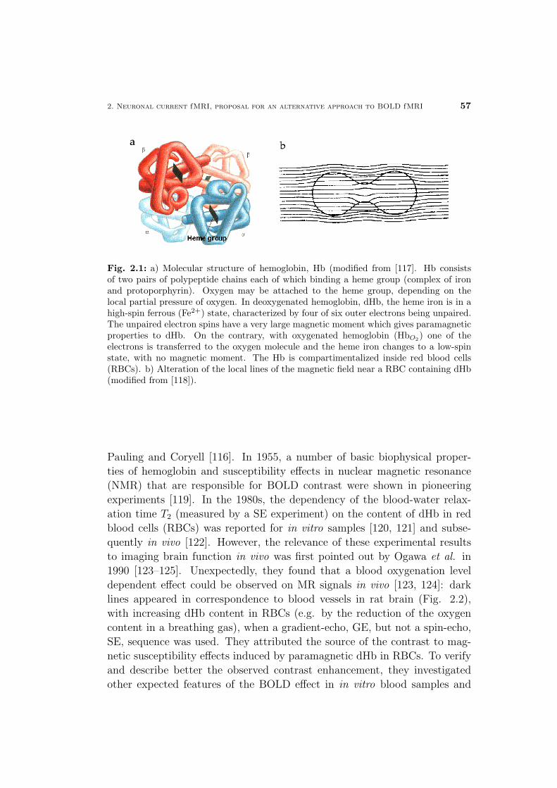
2. Neuronal current fMRI, proposal for an alternative approach to BOLD fMRI 57
Fig. 2.1: a) Molecular structure of hemoglobin, Hb (modified from [117]. Hb consistsof two pairs of polypeptide chains each of which binding a heme group (complex of ironand protoporphyrin). Oxygen may be attached to the heme group, depending on thelocal partial pressure of oxygen. In deoxygenated hemoglobin, dHb, the heme iron is in ahigh-spin ferrous (Fe2+) state, characterized by four of six outer electrons being unpaired.The unpaired electron spins have a very large magnetic moment which gives paramagneticproperties to dHb. On the contrary, with oxygenated hemoglobin (HbO2) one of theelectrons is transferred to the oxygen molecule and the heme iron changes to a low-spinstate, with no magnetic moment. The Hb is compartimentalized inside red blood cells(RBCs). b) Alteration of the local lines of the magnetic field near a RBC containing dHb(modified from [118]).
Pauling and Coryell [116]. In 1955, a number of basic biophysical proper-
ties of hemoglobin and susceptibility effects in nuclear magnetic resonance
(NMR) that are responsible for BOLD contrast were shown in pioneering
experiments [119]. In the 1980s, the dependency of the blood-water relax-
ation time T2 (measured by a SE experiment) on the content of dHb in red
blood cells (RBCs) was reported for in vitro samples [120, 121] and subse-
quently in vivo [122]. However, the relevance of these experimental results
to imaging brain function in vivo was first pointed out by Ogawa et al. in
1990 [123–125]. Unexpectedly, they found that a blood oxygenation level
dependent effect could be observed on MR signals in vivo [123, 124]: dark
lines appeared in correspondence to blood vessels in rat brain (Fig. 2.2),
with increasing dHb content in RBCs (e.g. by the reduction of the oxygen
content in a breathing gas), when a gradient-echo, GE, but not a spin-echo,
SE, sequence was used. They attributed the source of the contrast to mag-
netic susceptibility effects induced by paramagnetic dHb in RBCs. To verify
and describe better the observed contrast enhancement, they investigated
other expected features of the BOLD effect in in vitro blood samples and
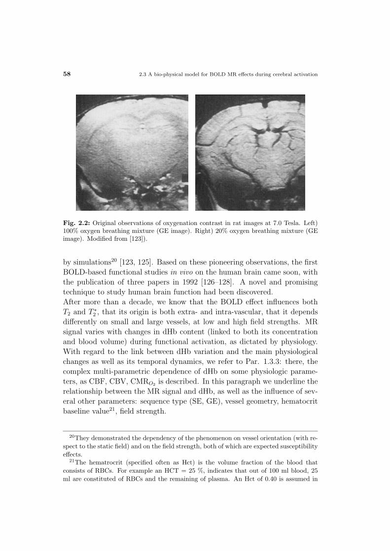
58 2.3 A bio-physical model for BOLD MR effects during cerebral activation
Fig. 2.2: Original observations of oxygenation contrast in rat images at 7.0 Tesla. Left)100% oxygen breathing mixture (GE image). Right) 20% oxygen breathing mixture (GEimage). Modified from [123]).
by simulations20 [123, 125]. Based on these pioneering observations, the first
BOLD-based functional studies in vivo on the human brain came soon, with
the publication of three papers in 1992 [126–128]. A novel and promising
technique to study human brain function had been discovered.
After more than a decade, we know that the BOLD effect influences both
T2 and T ∗2 , that its origin is both extra- and intra-vascular, that it depends
differently on small and large vessels, at low and high field strengths. MR
signal varies with changes in dHb content (linked to both its concentration
and blood volume) during functional activation, as dictated by physiology.
With regard to the link between dHb variation and the main physiological
changes as well as its temporal dynamics, we refer to Par. 1.3.3: there, the
complex multi-parametric dependence of dHb on some physiologic parame-
ters, as CBF, CBV, CMRO2 is described. In this paragraph we underline the
relationship between the MR signal and dHb, as well as the influence of sev-
eral other parameters: sequence type (SE, GE), vessel geometry, hematocrit
baseline value21, field strength.
20They demonstrated the dependency of the phenomenon on vessel orientation (with re-spect to the static field) and on the field strength, both of which are expected susceptibilityeffects.
21The hematrocrit (specified often as Hct) is the volume fraction of the blood thatconsists of RBCs. For example an HCT = 25 %, indicates that out of 100 ml blood, 25ml are constituted of RBCs and the remaining of plasma. An Hct of 0.40 is assumed in
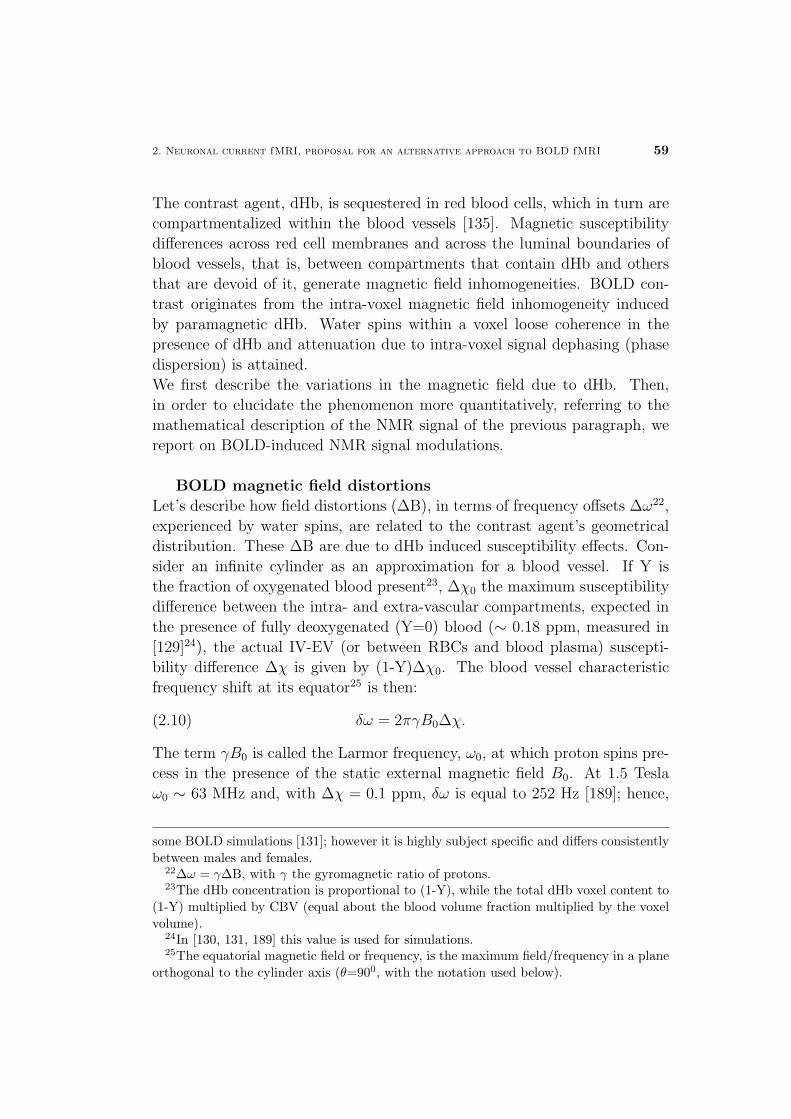
2. Neuronal current fMRI, proposal for an alternative approach to BOLD fMRI 59
The contrast agent, dHb, is sequestered in red blood cells, which in turn are
compartmentalized within the blood vessels [135]. Magnetic susceptibility
differences across red cell membranes and across the luminal boundaries of
blood vessels, that is, between compartments that contain dHb and others
that are devoid of it, generate magnetic field inhomogeneities. BOLD con-
trast originates from the intra-voxel magnetic field inhomogeneity induced
by paramagnetic dHb. Water spins within a voxel loose coherence in the
presence of dHb and attenuation due to intra-voxel signal dephasing (phase
dispersion) is attained.
We first describe the variations in the magnetic field due to dHb. Then,
in order to elucidate the phenomenon more quantitatively, referring to the
mathematical description of the NMR signal of the previous paragraph, we
report on BOLD-induced NMR signal modulations.
BOLD magnetic field distortions
Let’s describe how field distortions (∆B), in terms of frequency offsets ∆ω22,
experienced by water spins, are related to the contrast agent’s geometrical
distribution. These ∆B are due to dHb induced susceptibility effects. Con-
sider an infinite cylinder as an approximation for a blood vessel. If Y is
the fraction of oxygenated blood present23, ∆χ0 the maximum susceptibility
difference between the intra- and extra-vascular compartments, expected in
the presence of fully deoxygenated (Y=0) blood (∼ 0.18 ppm, measured in
[129]24), the actual IV-EV (or between RBCs and blood plasma) suscepti-
bility difference ∆χ is given by (1-Y)∆χ0. The blood vessel characteristic
frequency shift at its equator25 is then:
(2.10) δω = 2πγB0∆χ.
The term γB0 is called the Larmor frequency, ω0, at which proton spins pre-
cess in the presence of the static external magnetic field B0. At 1.5 Tesla
ω0 ∼ 63 MHz and, with ∆χ = 0.1 ppm, δω is equal to 252 Hz [189]; hence,
some BOLD simulations [131]; however it is highly subject specific and differs consistentlybetween males and females.
22∆ω = γ∆B, with γ the gyromagnetic ratio of protons.23The dHb concentration is proportional to (1-Y), while the total dHb voxel content to
(1-Y) multiplied by CBV (equal about the blood volume fraction multiplied by the voxelvolume).
24In [130, 131, 189] this value is used for simulations.25The equatorial magnetic field or frequency, is the maximum field/frequency in a plane
orthogonal to the cylinder axis (θ=900, with the notation used below).
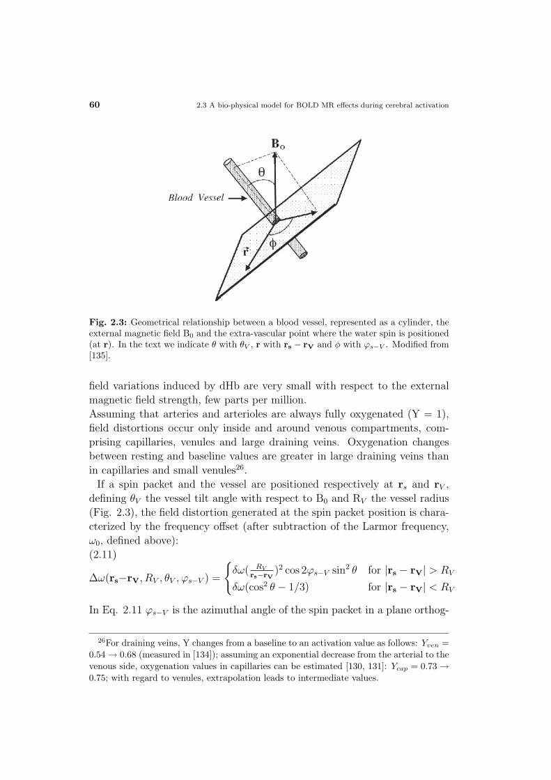
60 2.3 A bio-physical model for BOLD MR effects during cerebral activation
Fig. 2.3: Geometrical relationship between a blood vessel, represented as a cylinder, theexternal magnetic field B0 and the extra-vascular point where the water spin is positioned(at r). In the text we indicate θ with θV , r with rs − rV and φ with ϕs−V . Modified from[135].
field variations induced by dHb are very small with respect to the external
magnetic field strength, few parts per million.
Assuming that arteries and arterioles are always fully oxygenated (Y = 1),
field distortions occur only inside and around venous compartments, com-
prising capillaries, venules and large draining veins. Oxygenation changes
between resting and baseline values are greater in large draining veins than
in capillaries and small venules26.
If a spin packet and the vessel are positioned respectively at rs and rV ,
defining θV the vessel tilt angle with respect to B0 and RV the vessel radius
(Fig. 2.3), the field distortion generated at the spin packet position is chara-
cterized by the frequency offset (after subtraction of the Larmor frequency,
ω0, defined above):
(2.11)
∆ω(rs−rV, RV , θV , ϕs−V ) =
δω( RV
rs−rV)2 cos 2ϕs−V sin2 θ for |rs − rV| > RV
δω(cos2 θ − 1/3) for |rs − rV| < RV
In Eq. 2.11 ϕs−V is the azimuthal angle of the spin packet in a plane orthog-
26For draining veins, Y changes from a baseline to an activation value as follows: Yven =0.54 → 0.68 (measured in [134]); assuming an exponential decrease from the arterial to thevenous side, oxygenation values in capillaries can be estimated [130, 131]: Ycap = 0.73 →0.75; with regard to venules, extrapolation leads to intermediate values.
2. Neuronal current fMRI, proposal for an alternative approach to BOLD fMRI 61
onal to that cylinder; note that, as first approximation, the intravascular
magnetic field was considered approximately homogeneous27. If the vessel
is oriented parallel to the external static magnetic field, spins don’t experi-
ence any frequency offset. The vessel radius RV increases from capillaries
to large draining veins, being around 3-5 µm for capillaries (mean diameter
around 5 measured by [137]), 10-50 µm for small venules [138], and larger
for metavenules and large veins [130, 137, 139].
If more than one vessel (e.g. N) are present in a voxel, the local frequency
offset in the precession of each spin will be given by the sum of each vessel
contribution. Introducing an additional time dependence of spin positions
with respect to the static vessel geometry, to account for possible spin motion,
the frequency offset of water spins experiencing the dHb induced gradients
can be written as follows, with ∆ω(rs − rV, RV , θV , ϕs−V ) drawn from Eq.
2.11 :
(2.12) ∆ω(r(t)) =N∑
n=1
∆ω(rs(t)− rVn, RV n, θV n, ϕs−V n)
In summary, in this subparagraph it was shown how magnetic field distor-
tions are related to vessel geometry, vessel size and their oxygenation content.
How these field distortions affect the NMR signal is explained in the follow-
ing paragraph.
BOLD NMR signal modulations
In this paragraph it is explained how the BOLD signal depends on the mag-
netic field distortion generated by dHb, as well as on spin motion, sequence
type and field strength.
As shown in Par. 2.2 (Eq. 2.6), the induced magnetic field distortions locally
affect the phase of each spin, leading to spin dephasing and signal loss: with
regard to the specific case of BOLD effects, the time-dependent frequency
offset ∆ωk(r(t)) of Eq. 2.6 can be more explicitly written with respect to the
vascular geometry and spin motion by the use of Eq. 2.12.
With a decrease in the dHb content, a reduction in the dephasing between
spins occurs and consequently an increase in the signal magnitude is observed
27In practice, especially for large vessels, this is not the case and two intra-vascularcompartments are considered: the red blood cells and plasma; in this case the hematocritbecomes a crucial parameter for the BOLD effect and modulates its baseline value. Therelations in Eq. 2.11 were first described by Ogawa et al. [123–125], but in this moreprecise form only in [136].

62 2.3 A bio-physical model for BOLD MR effects during cerebral activation
(due to a rise of the Tapp2 , or of the T∗
2). With regard to the phase, a dHb
drop may lead to a net phase decreasing towards the net phase Φtis in absence
of dHb. This happens during cerebral activation, for instance in the second
(and most observed) phase of the BOLD hemodynamic response described
in Par. 1.3.3. The opposite effect, for total dHb increases which lead to the
initial dip and the final undershoot of the BOLD response, is also described
in Par. 1.3.3.
Unless a big vessel is present in a voxel, the observed BOLD signal changes
are greater in magnitude than in phase: for randomly oriented vessels, the
net phase changes is around zero, whereas an oriented vessel produces ob-
servable phase changes [149].
The radius of the field-creating particle is here the vessel radius RV for EV
effects, or the radius of RBCs for IV effects, primarily for large vessels. Small
and large vessels contribute differently to the BOLD signal, due to the two av-
eraging effects described in Par. 2.2. As explained above, capillaries, venules
and large draining veins all contribute to BOLD signal changes. However,
due to their small radii, for capillaries and small venules, diffusion effects
dominate both the extravascular and the intravascular28 signal contribution
and can be detected by both SE and GE sequences29. For larger venules and
draining veins, the static averaging domain is dominant for both extravascu-
lar and intravascular signal changes, which however can be detected only by
GE sequences. Intravascularly some dynamic averaging effects due to diffu-
sion will still be present around RBCs and some small signal changes will be
measured in large veins even if SE sequences are used, see Fig. 2.4.
Ogawa et al. [136] simulated the intravoxel dephasing, relative only to
the extravascular compartments, with a Monte-Carlo approach. Accord-
ing to the aforementioned theoretical considerations (see pag. 47), they
predicted a linear (quadratic) relationship between the relaxation rate R∗2
changes (∆R∗2 = ∆(1/T ∗
2 )) with large (small) vessels, as follows:
(2.13)
R∗
2 = αδωbLv for large vessels
R∗2 = η(δω)2bSvp for small vessels
28The intravascular dynamic averaging effects due to diffusion lead to a decreased bloodT2. Blood T2 decreases quadratically with field strength, as expected from diffusing spinsin the presence of field gradients. The impact of dHb on the transverse relaxation changesof in vitro and in vivo blood is measured in [120] and in [122], respectively. Li et al. [145],instead, measure T∗
2 changes in vivo (GE sequence).29However, by analytical modeling, in [189] it was shown that diffusion effects are neg-
ligible for GE sequences at 1.5 Tesla, while in the SE acquisitions they are much stronger.

2. Neuronal current fMRI, proposal for an alternative approach to BOLD fMRI 63
Fig. 2.4: Dynamic and static averaging regimes based on the diffusion distance relativeto the size of the compartment containing dHb. The dynamic averaging for extra-vascularspins around big vessels does not occur, since their diffusion distances are not large com-pared to vessel radius. Modified from [135].
where α and η are constants, δω is the frequency shift due to the susceptibi-
lity difference between the IV and the EV compartments, defined in Eq. 2.10,
bLv and bSv are the blood volume of large and small vessels, respectively, and
p is the fraction of active small vessels (referring to a capillary recruitment
model). The equations in Eq. 2.13 also define a direct linear relationship, for
the extravascular compartment, between blood volume and R∗2, with blood
volume increases matched by extravascular signal decreases30.
The contrast given by big vessels is higher, due to both their greater oxygena-
tion changes from the resting to the activated conditions (see above), and
to the greater effects due to static rather than dynamic averaging. However,
small vessels have one big advantage: they guarantee high spatial specificity
with respect to the location of the neuronal event, while signal changes due
to draining veins can occur several mm from the activation source. Due to
the quadratic dependence of the signal changes relative to diffusion effects
with field strength, high field MR scanners (≥ 4T) can be employed together
with the use of SE sequences to select only extravascular contributions close
30For the IV compartment, only if blood T2 is shorter than the EV tissues T2, anincrease in blood volume leads to a signal decrease, the opposite being true for longer T2.

64 2.3 A bio-physical model for BOLD MR effects during cerebral activation
to small vessels31, in order to attain the highest specificity. For a given TE
and with increasing field strength, the IV contributions tend indeed to zero,
due to the concurrent rapid decrease of blood T2. On the other hand, model
accuracy at low fields are mostly limited by the IV contribution of large ves-
sels. For B0 fields lower than 4 Tesla, SE echo sequences alone enable the
discrimination of the small vessel effects; however, both the EV and the IV
compartments contribute. For these reasons several approaches have been
proposed to selectively suppress IV effects at low fields32. New insight into
vascular geometric parameters is provided by the recent development of veno-
graphic techniques [150], which at present enable the discrimination of large
vessels (radius about 200 µm at 1.5 T and even smaller at higher fields); they
are also based on the use of both phase and amplitude images but require the
acquisition of high resolution images in addition to the BOLD fMRI images.
Several efforts have been made to model the many aspects of the BOLD
effect which, as discussed above, are based on a complex interplay between
vessel geometry/size/density, oxygenation, field strength, sequence type, and
static and diffusion effects. Most articles in the literature to date, describe
primarily gradient-echo BOLD effects at low fields and compare the IV versus
the EV effects, to determine which compartment mainly affects the BOLD
signal. For instance, EV spin dephasing around capillaries and veins, in
blood perfused parenchyma or around larger vessels, are described by theo-
retical models using Monte-Carlo simulations in [130, 136]33 and by analytical
models, such as in [139] (for the static averaging regime), and in [151, 189]
(for the contribution of diffusion effects)34. When comparing models and
IV/EV contributions with in vivo results, controversial findings were ob-
tained. Hoogenraad et al. [131] reported a huge impact of EV dephasing
around large vessels in in vivo measurements at 1.5 T. On the contrary, the
role of IV phase changes at low fields was emphasized in [130, 154] and the
31It is true that the higher the field strength, the greater the diffusion effects with respectto the static averaging effects; however, inhomogeneities induced by the contrast agent arealso greater at higher fields (see Eq. 2.10), and dynamic averaging will occur for a smallervessel size, with respect to lower fields.
32At these fields, the use of bipolar, also called diffusion-weighted, gradients can suppressthe IV effects with respect to different vessel sizes [130, 146–148]. In other approaches,large vessel contributions are suppressed by the use of phase images acquired concurrentlywith BOLD amplitude images [149].
33In [130] a comparison with the IV effects is performed.34In [139, 189] results relative to the slow diffusion approximation are shown; in [151]
the authors deal with diffusion effects in the narrowing regime.

2. Neuronal current fMRI, proposal for an alternative approach to BOLD fMRI 65
importance of venous structures was also outlined in [152, 153]. Neverthe-
less, with regard to high fields, many results consistently confirmed that for
SE acquisitions the BOLD signal has an EV origin around small vessels only
[155, 156], while for GE sequences (and long TEs), the signal is generated
from EV spins around both small and large vessels [156].
In the next paragraph we discuss briefly some features of BOLD fMRI ap-
proach, in terms of resolution, specificity and quantification/interpretation.
2.4 Mapping brain function by conventional
BOLD-based fMRI approaches: advan-
tages and limitations
Since its inception, BOLD fMRI has been adopted as the preferred tool to
map brain cognitive and sensory-motor functions. The smallest cortical field
activation detectable by this functional technique regards dHb changes per-
ceivable beyond the noise of one BOLD fMRI voxel (linear dimension around
1-5 mm). The fastest response, in principle, would be that obtained within
the acquisition of one slice (around 100 ms)35.
The question is whether the ultimate spatial and temporal resolutions at-
tained by fMRI are limited by the hardware and signal-to-noise ratio or are
limited by the physiology.
BOLD fMRI spatial resolution is only limited by the lack of specificity for
local activation-related phenomena. The most severe localization problem
in fMRI studies from the beginning is created by the draining vein effect.
Changes in blood oxygenation which travel down the vascular tree, with
time, may cross a substantial distance (many mm) from the site of activa-
tion, see Fig. 2.5. Nevertheless, valid strategies to suppress these undesired
effects (the use of SE sequences at high fields or the use of bipolar-gradients
or phase images at low fields) have been proposed, as discussed in the previ-
ous paragraph36.
Temporal resolution is instead limited by the hemodynamic response time
35However, in order to discern a stimulus related signal, averaging or regression tech-niques based on multiple acquisition of the hemodynamic response are usually employed,with an fMRI session lasting few minutes.
36Perfusion imaging also avoids large vessel contribution, both at low and at high fields,since it is specific to capillary micro-circulation. For a review of the accuracy of GE- SE-and perfusion-techniques with regard to neuronal activation see [157].
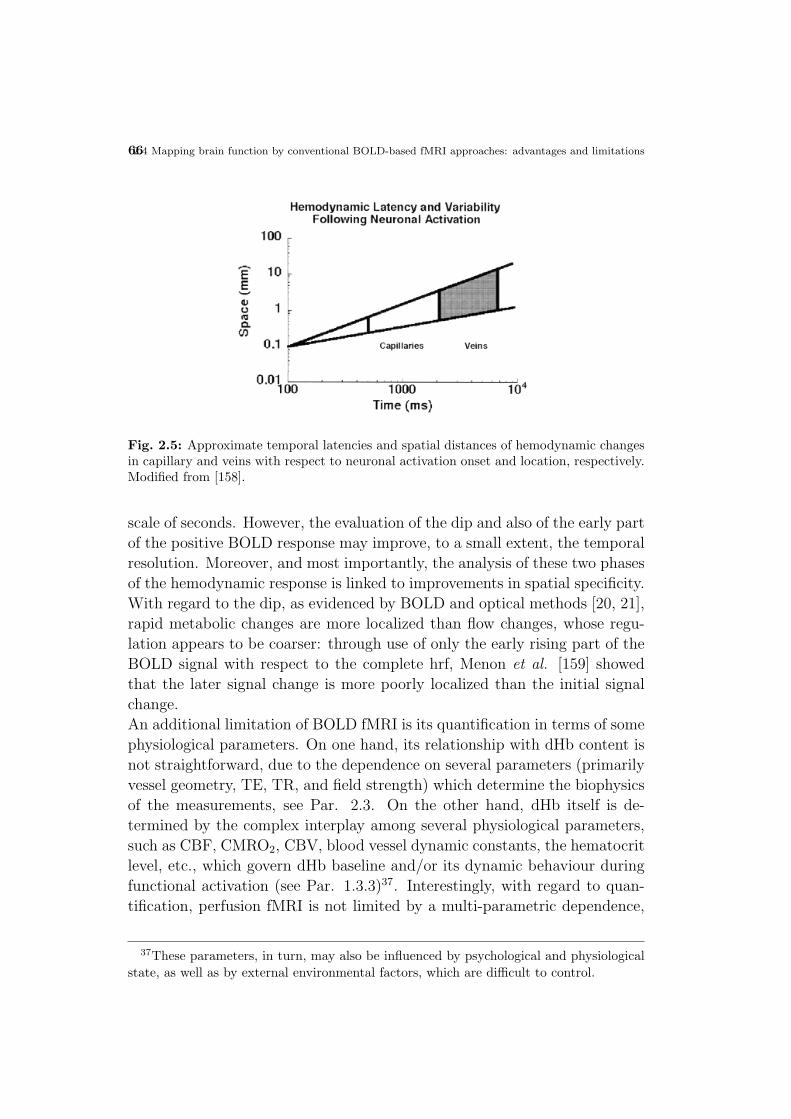
662.4 Mapping brain function by conventional BOLD-based fMRI approaches: advantages and limitations
Fig. 2.5: Approximate temporal latencies and spatial distances of hemodynamic changesin capillary and veins with respect to neuronal activation onset and location, respectively.Modified from [158].
scale of seconds. However, the evaluation of the dip and also of the early part
of the positive BOLD response may improve, to a small extent, the temporal
resolution. Moreover, and most importantly, the analysis of these two phases
of the hemodynamic response is linked to improvements in spatial specificity.
With regard to the dip, as evidenced by BOLD and optical methods [20, 21],
rapid metabolic changes are more localized than flow changes, whose regu-
lation appears to be coarser: through use of only the early rising part of the
BOLD signal with respect to the complete hrf, Menon et al. [159] showed
that the later signal change is more poorly localized than the initial signal
change.
An additional limitation of BOLD fMRI is its quantification in terms of some
physiological parameters. On one hand, its relationship with dHb content is
not straightforward, due to the dependence on several parameters (primarily
vessel geometry, TE, TR, and field strength) which determine the biophysics
of the measurements, see Par. 2.3. On the other hand, dHb itself is de-
termined by the complex interplay among several physiological parameters,
such as CBF, CMRO2, CBV, blood vessel dynamic constants, the hematocrit
level, etc., which govern dHb baseline and/or its dynamic behaviour during
functional activation (see Par. 1.3.3)37. Interestingly, with regard to quan-
tification, perfusion fMRI is not limited by a multi-parametric dependence,
37These parameters, in turn, may also be influenced by psychological and physiologicalstate, as well as by external environmental factors, which are difficult to control.

2. Neuronal current fMRI, proposal for an alternative approach to BOLD fMRI 67
since it is only affected by CBF, and with some additional measurements (T1
for each voxel) it can furnish quantitative information regarding blood flow.
Finally, the lack of a quantification limits a precise interpretation of fMRI
maps for single subject investigations and may generate lower sensitivity
in group analyzes. Indeed, for the same stimulus but in different subjects,
variations in the mentioned parameters as well in the neural response, or
in the baseline metabolic values, affect both the shape and the intensity of
the hemodynamic response of each investigated volunteer. For this reason,
the absence of quantification translates into poorer inter-subject compar-
isons (group analyses [160–162]), which are extensively employed in studies
regarding brain mapping and in cognitive neuro-science investigations. Nev-
ertheless, to quantify BOLD effects several supplementary measurements of
physiological parameters are needed. With regard to the deoxyhemoglobin
content determination, both vessel geometry and CBV knowledge are cru-
cial: for this aim high-resolution venography and CBV perfusion fMRI may
be employed concurrent with the BOLD acquisition. Also the measurement
of the hematocrit value is fundamental for quantification, since it enables a
better definition of the signal baseline. For a more general delineation of the
physiological response of the subject, the use of perfusion fMRI acquisitions
to independently measure CBF, and valid calibration methods for CMRO2
estimation would also be helpful.
Moreover, quantification is not only limited by the knowledge of physiology,
but also by the acquisition itself. For instance, acquisition parameters (TR,
TE) may introduce confounding effects: short TRs may introduce unwanted
inflow effects of large arteries38; conversely, the TE (and also the T1) mod-
ulates the signal in terms of its ratio with the relaxation time at rest (see
Eq. 2.4, giving excellent results for one region or subject but poor results for
others. Multi-echo approaches may solve the delicate interplay between the
choice of TE and the different baseline T2,2∗, as well as the inflow artifact,
as proposed in [163, 164].
38An unwanted phenomenon that may be present in activation maps is the so-calledinflow effect in the blood compartment. It is due to fresh spins flowing into the voxelduring it signal acquisition and results in changes in %BL in Eq. 2.4, which may lead tovariation in the signal magnitude (the sign and the amplitude depend on the sequencetype, SE or GE, and on the vessel size, depending on blood velocities and on acquisitionparameters, such as the TE or the TR).
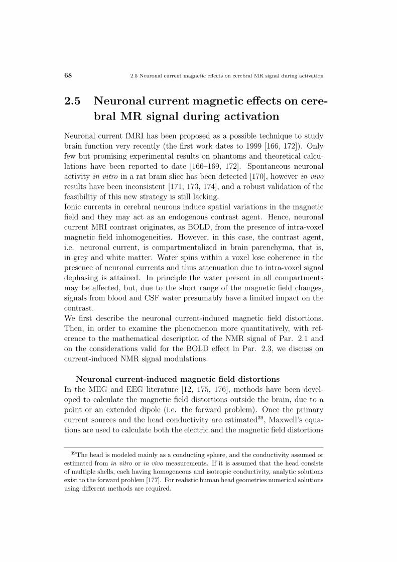
68 2.5 Neuronal current magnetic effects on cerebral MR signal during activation
2.5 Neuronal current magnetic effects on cere-
bral MR signal during activation
Neuronal current fMRI has been proposed as a possible technique to study
brain function very recently (the first work dates to 1999 [166, 172]). Only
few but promising experimental results on phantoms and theoretical calcu-
lations have been reported to date [166–169, 172]. Spontaneous neuronal
activity in vitro in a rat brain slice has been detected [170], however in vivo
results have been inconsistent [171, 173, 174], and a robust validation of the
feasibility of this new strategy is still lacking.
Ionic currents in cerebral neurons induce spatial variations in the magnetic
field and they may act as an endogenous contrast agent. Hence, neuronal
current MRI contrast originates, as BOLD, from the presence of intra-voxel
magnetic field inhomogeneities. However, in this case, the contrast agent,
i.e. neuronal current, is compartmentalized in brain parenchyma, that is,
in grey and white matter. Water spins within a voxel lose coherence in the
presence of neuronal currents and thus attenuation due to intra-voxel signal
dephasing is attained. In principle the water present in all compartments
may be affected, but, due to the short range of the magnetic field changes,
signals from blood and CSF water presumably have a limited impact on the
contrast.
We first describe the neuronal current-induced magnetic field distortions.
Then, in order to examine the phenomenon more quantitatively, with ref-
erence to the mathematical description of the NMR signal of Par. 2.1 and
on the considerations valid for the BOLD effect in Par. 2.3, we discuss on
current-induced NMR signal modulations.
Neuronal current-induced magnetic field distortions
In the MEG and EEG literature [12, 175, 176], methods have been devel-
oped to calculate the magnetic field distortions outside the brain, due to a
point or an extended dipole (i.e. the forward problem). Once the primary
current sources and the head conductivity are estimated39, Maxwell’s equa-
tions are used to calculate both the electric and the magnetic field distortions
39The head is modeled mainly as a conducting sphere, and the conductivity assumed orestimated from in vitro or in vivo measurements. If it is assumed that the head consistsof multiple shells, each having homogeneous and isotropic conductivity, analytic solutionsexist to the forward problem [177]. For realistic human head geometries numerical solutionsusing different methods are required.

2. Neuronal current fMRI, proposal for an alternative approach to BOLD fMRI 69
Fig. 2.6: Schematic representation of the parameters involved in the calculation of thefield B(r) due to a dipole Q at position rQ. In the text B(r) is indicated as ∆B(r− r′).Modified from [168].
induced by neuronal activity. In particular, they are applied in the quasi-
static regime, which holds, considering the conductivity and the geometry
of human brain, for frequencies of current variation manifested in neuronal
synaptic activity (< 100 Hz) [175]. 40.
For the neuronal current MRI approach these calculations have to be ex-
tended to the magnetic field changes inside a sphere due to a non-point
dipole. Indeed MRI measures local changes in the magnetic field, at a few
mm from the current source, contrary to MEG and EEG recordings which
are made on the scalp, at several cm away from it. Both primary and volume
currents are in principle of interest and the magnetic field distribution close
to and within the current source must be worked out.
Let’s assume that the head is a sphere of radius RH and conductivity σ,
surrounded by a medium with zero conductivity; a point current dipole of
moment Q41 is located at position rQ with respect to the center of the sphere
(Fig. 2.6). The primary (Jp) and the passive volume (Jv) current distribu-
tion at position r′ pertaining to the sphere are then respectively:
(2.14)
Jp(r′) = Qδ(r′ − rQ);
Jv(r′) = σE(r′) = −σ∇V(r′);
40In this case, for the calculation of both the electric E and magnetic field B, their timevariations (dE/dt, dB/dt) can be ignored as source terms.
41The letter Q is used here to avoid confusion with p, the symbol for a charge dipole.

70 2.5 Neuronal current magnetic effects on cerebral MR signal during activation
where δ(r) is the Dirac delta function, E and V are the electric field and
potential, respectively, produced by the current dipole, and∇ is the Gradient
operator. The total current density due to the point dipole is hence given
by: J(r′) =Jp(r′) + Jv(r′).
The induced magnetic field ∆B at location r inside the sphere due to the
point current dipole can be calculated by the use of the Maxwell’s equations,
in the quasi-static regime. A convenient approach is to use the Ampere-
Laplace law for the field variations with respect to the static magnetic field
B0:
(2.15) ∆B(r− r′) =µ0
4π
∫V s
J(r′)× (r− r′)
(r− r′)3d3r′
where µ0 is the permeability of free space and Vs the sphere volume. Sub-
stituting the expression for the total current density J(r′) due to the point
dipole in Eq. 2.15, the so-called Geselowitz formula [178] is obtained, with
two separable and additive contributions to the magnetic field due to the
primary and volume currents, respectively:
(2.16)
∆B(r− r′) =µ0
4π(
∫V s
JP(r′)× (r− r′)
(r− r′)3d3r′ + σ
∫Ss
V(r′)(r− r′)
(r− r′)3× n(r′)dS ′)
where n(r′) is the unit vector perpendicular to the sphere surface Ss at posi-
tion r′. From Eq. 2.16, it can be seen that the effect of the volume currents
is the same as the effect of a surface current distribution, −σV (r′)n(r′), on
the surface of the sphere.
The frequency offset in the quadrature detection plane for each spin at po-
sition r will be influenced only by the components of the field variations
parallel to the external static magnetic field B0 (∆B(r− r′)‖), according to
the following relation:
(2.17) ∆ω(r− r′) = 2πγ∆B(r− r′)‖.
The components of the induced magnetic field perpendicular to B0 will have
a negligible effect. In other terms, considering Eq. 2.16, only the current
point dipole components perpendicular to B0 affect the MR signal.
If the current dipole is extended, to calculate the generated magnetic field
Eq. 2.14 has to be modified and the integral in Eq. 2.16 and hence in Eq.
2.17 computed over all r′ pertaining to the current dipole. Equivalently, the
extended dipole can be considered as n small point current dipoles, evenly
spread in three dimensions throughout the spatial extent of the primary
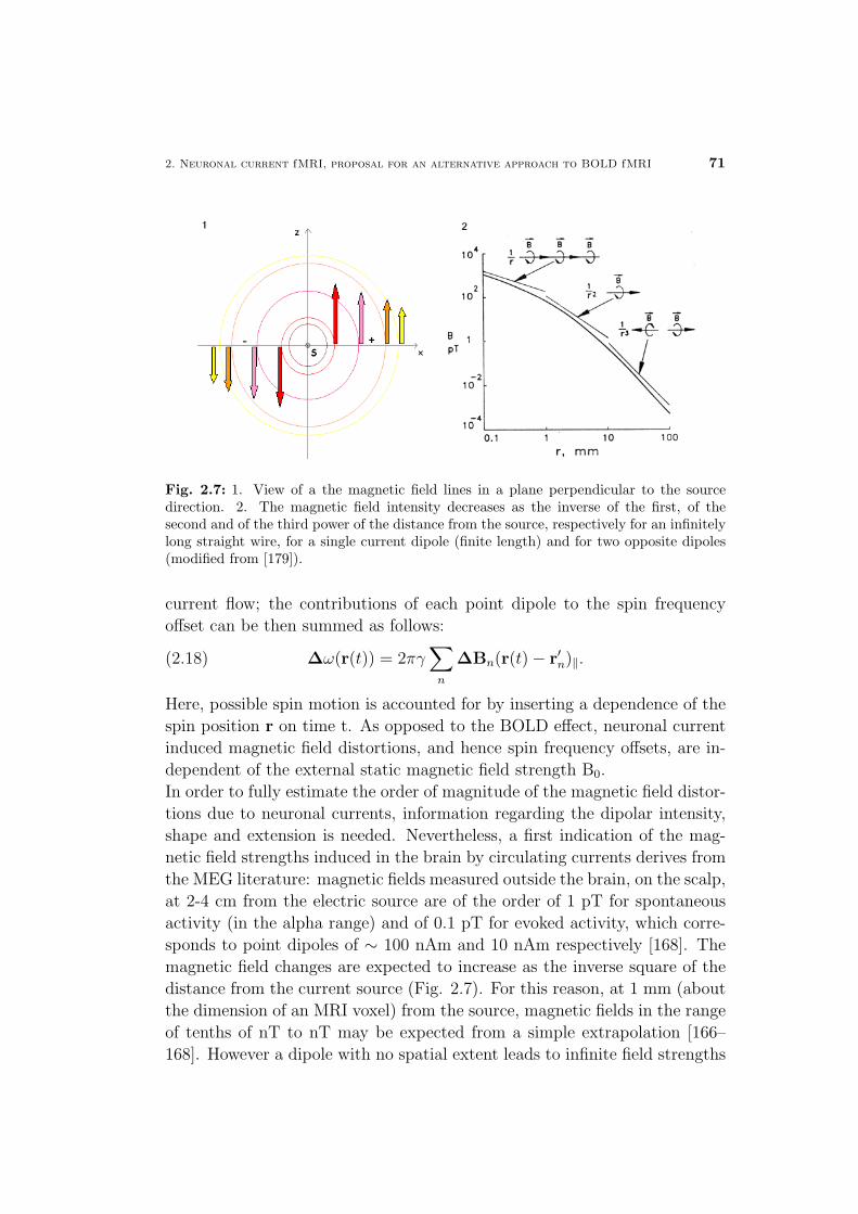
2. Neuronal current fMRI, proposal for an alternative approach to BOLD fMRI 71
Fig. 2.7: 1. View of a the magnetic field lines in a plane perpendicular to the sourcedirection. 2. The magnetic field intensity decreases as the inverse of the first, of thesecond and of the third power of the distance from the source, respectively for an infinitelylong straight wire, for a single current dipole (finite length) and for two opposite dipoles(modified from [179]).
current flow; the contributions of each point dipole to the spin frequency
offset can be then summed as follows:
(2.18) ∆ω(r(t)) = 2πγ∑
n
∆Bn(r(t)− r′n)‖.
Here, possible spin motion is accounted for by inserting a dependence of the
spin position r on time t. As opposed to the BOLD effect, neuronal current
induced magnetic field distortions, and hence spin frequency offsets, are in-
dependent of the external static magnetic field strength B0.
In order to fully estimate the order of magnitude of the magnetic field distor-
tions due to neuronal currents, information regarding the dipolar intensity,
shape and extension is needed. Nevertheless, a first indication of the mag-
netic field strengths induced in the brain by circulating currents derives from
the MEG literature: magnetic fields measured outside the brain, on the scalp,
at 2-4 cm from the electric source are of the order of 1 pT for spontaneous
activity (in the alpha range) and of 0.1 pT for evoked activity, which corre-
sponds to point dipoles of ∼ 100 nAm and 10 nAm respectively [168]. The
magnetic field changes are expected to increase as the inverse square of the
distance from the current source (Fig. 2.7). For this reason, at 1 mm (about
the dimension of an MRI voxel) from the source, magnetic fields in the range
of tenths of nT to nT may be expected from a simple extrapolation [166–
168]. However a dipole with no spatial extent leads to infinite field strengths

72 2.5 Neuronal current magnetic effects on cerebral MR signal during activation
Fig. 2.8: Section of the extended current dipole employed in [168] for simulations. Theevenly distributed point dipoles are indicated with ·, while the points where the magneticfield is sampled with ×. Modified from [168].
at zero distance between the dipole and the measurement point and is not a
realistic model.
For this reason simulations of an active area of the cortex containing dipolar
currents parallel to each other were made by Konn et al. [168], represen-
tative of thousands of tiny oriented dendritic shafts. These authors took
into account only the static effects, measurable by a GE acquisition. An
extended current dipole of total moment Q, was calculated by summing the
contributions from n point current dipoles, each of moment Q/n, distributed
uniformly in three dimensions throughout the current spatial extent (see
Fig. 2.8). Each point dipole was separated by 0.1 mm (although also diffe-
rent spacings were explored, changing the number of point dipoles n, with
little impact on the magnetic field calculated). Calculations were performed
for a point dipole and for dipoles of spatial extents of 3x3x2 mm3 and 6x6x2
mm3. Konn et al. found that a 3x3x2 mm3 extended current dipole with Q
= 10 nAm strength, oriented in a plane orthogonal to B0, induces maximum
absolute magnetic field variations of 0.5 nT in the surrounding space due to
the primary current distribution and close to it. In addition these authors
found that volume currents effects are negligible close to the dipole (< 1cm)
and are around 1 pT at the sphere surface for a dipole distant 3 cm from the
sphere surface42 (see Fig. 2.9). Hence the detectability of neuronal currents
is dictated by primary, rather than volume currents, for a realistically posi-
42For a dipole 1 cm far from the conducting sphere surface, the maximum field variationsare increased by a factor of 10, but this value is still 2 orders of magnitude smaller thanthe peak value of the primary current induced maximum field change.
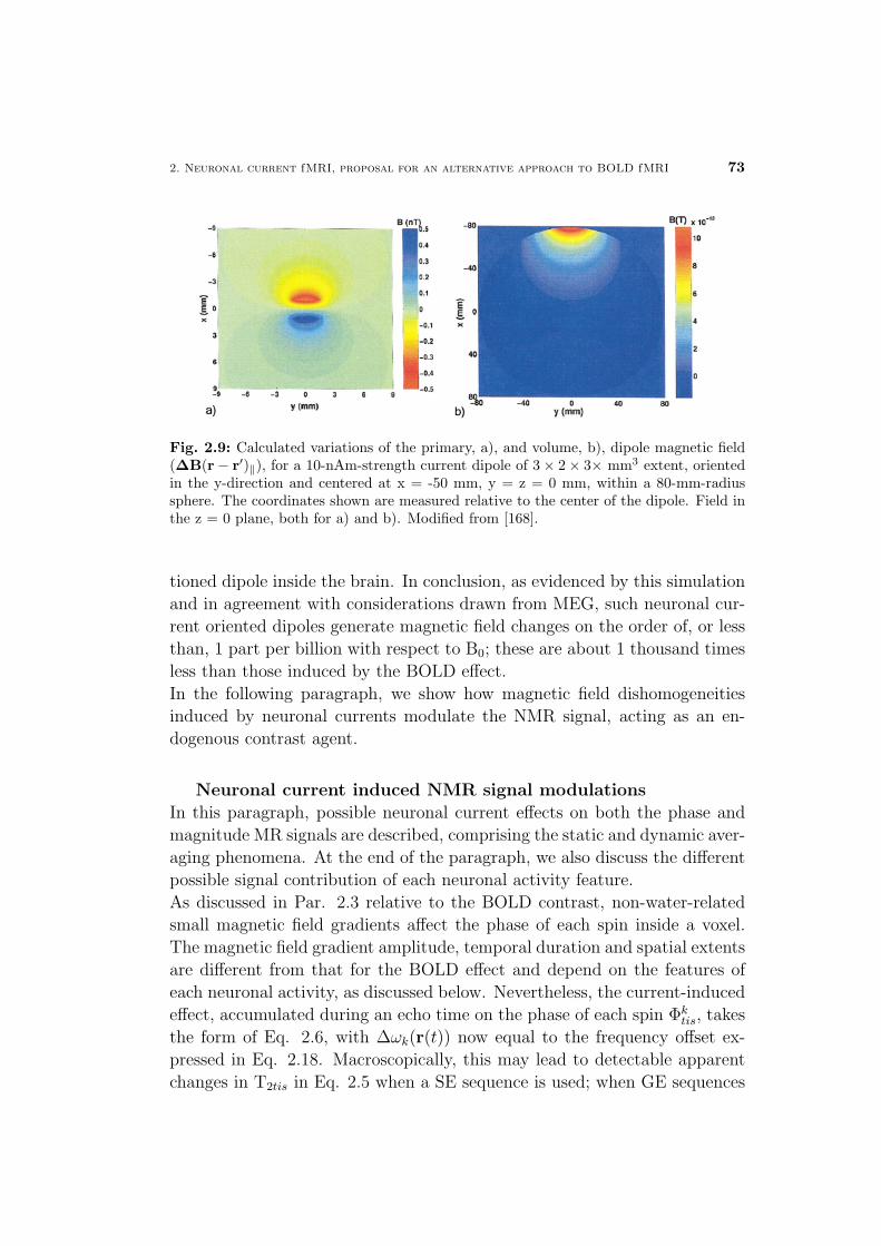
2. Neuronal current fMRI, proposal for an alternative approach to BOLD fMRI 73
Fig. 2.9: Calculated variations of the primary, a), and volume, b), dipole magnetic field(∆B(r− r′)‖), for a 10-nAm-strength current dipole of 3× 2× 3× mm3 extent, orientedin the y-direction and centered at x = -50 mm, y = z = 0 mm, within a 80-mm-radiussphere. The coordinates shown are measured relative to the center of the dipole. Field inthe z = 0 plane, both for a) and b). Modified from [168].
tioned dipole inside the brain. In conclusion, as evidenced by this simulation
and in agreement with considerations drawn from MEG, such neuronal cur-
rent oriented dipoles generate magnetic field changes on the order of, or less
than, 1 part per billion with respect to B0; these are about 1 thousand times
less than those induced by the BOLD effect.
In the following paragraph, we show how magnetic field dishomogeneities
induced by neuronal currents modulate the NMR signal, acting as an en-
dogenous contrast agent.
Neuronal current induced NMR signal modulations
In this paragraph, possible neuronal current effects on both the phase and
magnitude MR signals are described, comprising the static and dynamic aver-
aging phenomena. At the end of the paragraph, we also discuss the different
possible signal contribution of each neuronal activity feature.
As discussed in Par. 2.3 relative to the BOLD contrast, non-water-related
small magnetic field gradients affect the phase of each spin inside a voxel.
The magnetic field gradient amplitude, temporal duration and spatial extents
are different from that for the BOLD effect and depend on the features of
each neuronal activity, as discussed below. Nevertheless, the current-induced
effect, accumulated during an echo time on the phase of each spin Φktis, takes
the form of Eq. 2.6, with ∆ωk(r(t)) now equal to the frequency offset ex-
pressed in Eq. 2.18. Macroscopically, this may lead to detectable apparent
changes in T2tis in Eq. 2.5 when a SE sequence is used; when GE sequences
74 2.5 Neuronal current magnetic effects on cerebral MR signal during activation
are employed, variation in the T∗2tis may take place, which, in absence of
neuronal currents, is determined by the magnetic field gradients which are
already present. Also Φtis (Eq. 2.5) may be affected in both SE and GE
acquisitions. In brief, even if there is only one tissue type in a voxel, both
the magnitude and the phase signals of that voxel may be modulated by the
presence of neuronal currents, as can be seen from Eq. 2.3.
Depending on the geometry of the ensemble of active neurons, the contrast
due to the neuronal current flow will be greater in the phase or in magni-
tude images: if the microscopic dipoles are randomly oriented then there will
be no net phase change43; however, if dispersion between spin phases takes
place the magnitude of the signal will be affected. On the other hand, if there
are oriented dipoles, phase rather than magnitude images will be more influ-
enced. Accordingly, Konn et al. [168] showed by calculations for an extended
dipole constituted of oriented point dipoles that this is the case for dipole
intensities lower than a few µAm; for nAm current dipoles the phase changes
are five orders of magnitude greater than those in magnitude images44. The
latter considerations are valid, for instance, for oriented apical dendrites of
pyramidal neurons (see Par. 1.2.2) and hence relate to the generation of
E/IPSPs. For projectional axons macroscopic dipoles/quadrupoles (equiva-
lent of one big vessel for the BOLD effect) would also be generated and the
phase would be affected more than the magnitude. With regard to non ori-
ented cells inside an MR voxel, like non-pyramidal cells (stellate cells, etc.),
due to geometric considerations (radially oriented dendrites at random an-
gles), the contrast in the magnitude signal would instead probably be greater
than that in the phase45. In [171], Xiong et al. hypothesized that magnitude
changes should be more evident, however the authors considered only the exi-
stence or the predominance of randomly oriented cells (which actually is not
always the case, since the density ratio of the two types of neurons changes
between cortical layers, see Par. 1.2.2). However, no realistic simulations of
non-oriented cells have been presented yet in the literature.
As for BOLD, two averaging dephasing phenomena in the presence of ex-
43In general, a symmetric distribution of the induced magnetic field in a voxel leads toa net phase in that voxel equal to zero; so as for randomly oriented dipoles, as well as fora macroscopic and oriented dipole positioned exactly at the center of the voxel.
44The simulated voxel linear dimensions ranged from 0 to 10 mm. Furthermore, theyfound that the greater the extent of the current source, the lower the contrast for bothsignals.
45In this case, the generated magnetic field is said to be “closed” and it cannot bemeasured far from the cell, for instance by MEG.

2. Neuronal current fMRI, proposal for an alternative approach to BOLD fMRI 75
ternal static field inhomogeneities may give rise to changes in T∗2, Tapp
2 and
Φtis. Depending on the relative water diffusion lengths46 with respect to the
neuronal current induced gradient amplitude, static and dynamic averaging
may take place, with different MR signal contributions depending on the
sequence used (for instance, SE or GE). The radii of the cerebral dendrites
(gray matter) are of the order of tenths of µm to a few µm; axons may have
a greater radius, however ranging from 0.1 to 10 µm [3]47. Hence dynamic
averaging may be the predominant effect for each type of neuronal activity
and the contrast for SE and GE measurements may be very similar to each
other. No simulations of the neuronal current effects in the dynamic averag-
ing regime are yet available in the literature. In [168] simulations were made
only for static spins and lower induced magnetic field changes relative to that
found by the authors may be expected when considering the dynamic aver-
aging phenomena. Moreover, the definition of “static” for neuronal currents
may be inadequate: indeed it is typically defined for events lasting more than
a TE, which may not be the case for the dipolar component, observed for
instance in EEG and MEG measurements. When the neuronal current pri-
mary magnetic effects take place only during the first half of the echo time,
the “static” averaging effects will also contribute to SE measurements, since
they will not be refocused. This was achieved in our in vivo measurements,
by synchronizing the SE acquisition with the electric event, see Chap. 4.
Each type of neuronal activity (see Par. 1.2) may play a role for neuronal
current MRI, with contributions depending on the induced magnetic field
amplitude, its temporal duration and spatial extent. These characteristics
should also determine the feasibility of neuronal current detection by MRI.
We briefly discuss the possible neuronal current MRI contribution from each
of these different features of neuronal activity.
As already discussed in Par. 1.2.3, action potentials have greater amplitudes
than post-synaptic potentials. However, their short duration (about only 1
ms) and lack of synchronization imply no further gain in amplitude from, for
instance, summation of multiple synchronous spikes. Moreover, the electro-
magnetic field induced by action potentials decreases much more rapidly with
increasing distance (r) from the source than that relative to E/IPSPs: action
potentials (which can be represented by two subsequent and opposite dipoles)
have associated quadrupolar fields [9] (see Fig. 1.5), which decrease as r−3,
while postsynaptic potentials behave like single dipoles with field amplitudes
46In Par. 2.2 as a realistic reference for fMRI, an LD of ∼ 8µm was assumed.47The myelin sheath may enlarge the axon radius by several µm.

76 2.6 Potential benefits and shortcomings of neuronal current fMRI
directly proportional to r−2 (Fig. 2.7). These considerations imply that the
voxel signal variation due to action potentials, which is directly proportional
to the amplitude and the duration (up to a TE or TE/2 for a GE and SE
sequence, respectively) of the electric source, should be smaller than that
of post-synaptic potentials. Furthermore and most importantly, since MRI
measurements should be synchronized with the electric event in order to de-
tect it, perfect knowledge of the spiking activity timing would be optimal.
This may only be possible through use of intra-cortical recordings, which on
humans in vivo are not usually feasible.
On the contrary, concurrent recording of post-synaptic potentials (EPSPs
and IPSPs) may offer some advantages for neuronal current MRI: they are
long lasting (tenths of ms) and, while smaller in amplitude, can sum up
efficiently; moreover, their timing can be estimated by EEG and MEG re-
cordings, which are well developed non-invasive techniques. We have already
mentioned that some geometric considerations may favor pyramidal over non-
pyramidal neurons in their scalp detection by EEG and MEG. For neuronal
current MRI they both may in principle play a role in the contrast genera-
tion, since the measurement is local and accounts for microscopic changes in
the magnetic field. Moreover, as elucidated above, the activity of pyramidal
and non pyramidal cells may be different in their effects on the phase and
the magnitude of NMR signals.
In conclusion, like EEG and MEG recordings, neuronal current MRI may
have difficulty in detecting spiking activity; however, sub-threshold dendritic
activity of both pyramidal and non-pyramidal cells may contribute to the
neuronal current MRI signal.
2.6 Potential benefits and shortcomings of neu-
ronal current fMRI
Neuronal current MRI is an emerging functional contrast that may repre-
sent an appealing alternative to conventional blood-oxygen level dependent
(BOLD) methods. Neuronal currents may give more precise temporal infor-
mation than the sluggish hemodynamic response, since local magnetic field
effects vanish as the neuronal event ceases (tens of ms). Likewise, more pre-
cise spatial information may be obtained since local field variations fall off
with the square power of the distance from the dipolar source, while the
BOLD effect may extend to adjacent non-activated brain areas due to the
draining vein phenomenon. In summary, in contrast to the BOLD approach,

2. Neuronal current fMRI, proposal for an alternative approach to BOLD fMRI 77
for neuronal current fMRI, if feasible in vivo, hardware and signal-to-noise
ratio, rather than the electro-physiological response, would mainly limit the
ultimate temporal and spatial resolutions attained.
With regard to quantification, the contrast in neuronal current MRI is roughly
proportional to the dipolar amplitude, duration, geometry and to the inverse
of the spatial extent. However, a precise quantification is highly dependent
on model quality. In the present state of the art, only few realistic mod-
eling attempts have been made [168]; nevertheless, the use of experimental
evidence from other techniques, such as EEG, MEG and intra-cortical recor-
dings, will enable significant improvements in this endeavor.
In our opinion, there are three main issues to be solved in order to detect
primary magnetic effects due to neuronal currents by MRI. In the present
PhD thesis, these topics are addressed, by proposing acquisition approaches
and by experimental validation in both phantoms and in vivo (see next chap-
ters).
The first issue regards MRI sensitivity. Neuronal-current induced phase
changes are expected to be modest [166–168] with respect to the intrinsic
MR phase and amplitude noise. For this reason, MR sensitivity has to be
optimized, either by decreasing the noise or by increasing the signal change
itself. In a first work, we explored ways to increase the sensitivity by reduc-
tion of the phase noise. This may be achieved for instance by increasing the
static magnetic field strength. However, we show that optimized acquisition
strategies and improved hardware performance at low fields leads to results
close to that obtained at double field strengths. Using a phantom, we also
investigated the detection limit for neuronal current induced phase changes
in spin-echo images at 1.5 Tesla, by the use of optimized strategies (see Chap.
3). With regard to improvement of the expected signal changes, they may
be obtained by several means, e.g., by prolonging the duration and strength
of the neuronal event, by optimization of the geometrical characteristics of
the current dipole with respect to the externally applied magnetic field and
image voxel localization [168, 173] (see Chap. 4). For the neuronal current
contrast, no gain would be obtained by increasing the field strength.
The second question is related to spatio-temporal synchronization between
the neuronal event and the MR acquisition. An accurate synchronization
is also related to sensitivity, and more specifically to contrast optimization.
However we deal with this issue separately, since it is a supplementary techni-
cal issue. Temporal synchronization is needed to center the events of interest
in the acquisition window, both for GE and SE sequences. In addition, if a
SE sequence is used, it is also crucial in order to avoid refocusing of the effect

78 2.6 Potential benefits and shortcomings of neuronal current fMRI
of interest during acquisition. Beyond the temporal issues, dipolar spatial
knowledge is also needed in order to optimize the contrast. A method is pro-
posed for spatio-temporal synchronization of the two events and applied in
vivo on three subjects (see Chap. 4). It makes use of combined information
driven by the EEG, BOLD and neuronal current fMRI approaches.
The third problem consists of artifact control. Discrimination between pri-
mary neuronal effects and unwanted artifactual signal changes is a fundamen-
tal prerequisite for a successful application of neuronal current MRI. Both
movement and secondary hemodynamic-metabolic (BOLD) changes may be
the origin of possible artifacts. Two solutions to this problem are proposed
and adopted experimentally in the in vivo pilot study (see Chap. 4). They
both rely on an adequate sequence type and stimulation design.
In the next chapter, we start by evaluating MR sensitivity for the detection
of neuronal current primary magnetic effects.

Chapter 3
Optimization of neuronal
current fMRI sensitivity by
simulations and experiments on
a phantom
In this chapter, means through which pushing the limits of MRI sensitivity
for the detection of ultra-weak magnetic field changes are discussed. The
interest in detecting by MRI small magnetic field distortions comes from the
possibility to detect primary effects elicited by ionic currents during neuronal
activity.
Neuronal-current induced MR signal changes are indeed expected to be mod-
est [166–168] with respect to the intrinsic MR noise. To overcome this limit,
MR sensitivity can be optimized either by decreasing the noise or by increas-
ing the signal change itself. We treat the latter issue in the next chapter. In
the present chapter we explore ways to increase the sensitivity by improve-
ment of the MR noise figure. This may be achieved for instance by increasing
the static magnetic field strength. However, we show that optimized acqui-
sition strategies and improved hardware performance at low fields lead to
results close to that obtained at double field strengths. We also investigate
on a phantom the detection limit for neuronal current induced signal changes
in spin-echo phase images at 1.5 Tesla, by the use of optimized strategies.
The chapter is articulated as follows: we first review findings in literature
which report on the detection by MRI of ultra-weak magnetic field changes.
We then investigate possible advantages of multi-spin-echo imaging and eva-
luate how the information contained in the different echo images can be
79

80 3.1 MRI sensitivity for the detection of nTesla magnetic field changes
combined in order to increase signal temporal stability and hence the SNR.
Particularly, the limitations of the multi-echo approach with respect to the
conventional single echo method are analyzed theoretically in terms of the
time delay between subsequent echo images and the transverse relaxation
time. Experimentally, the result of some hardware settings on the phase
stability in single-echo images is also evaluated both by phantom measure-
ments and in vivo. Specifically the effect of improving the coil sensitivity
and the acquisition bandwidth is investigated. Finally, the detection limit
of current-induced phase changes at 1.5 Tesla is estimated experimentally
in phantom measurements, with temporal phase stability comparable to the
values found in the human brain. At this aim, electric currents were induced
in a wire-loop, placed perpendicularly to the external field, in synchrony with
the (multi)-spin-echo EPI acquisition. The detected phase changes were sub-
sequently quantified in terms of the associated magnetic field.
Parts of this work, regarding the detection limit and the multi-spin echo
acquisition strategy, have been published in [169, 182], respectively.
3.1 MRI sensitivity for the detection of nTesla
magnetic field changes
We saw in Par. 2.5 that by the solution of the inverse MEG problem [166–168]
or by direct calculations [168], expected magnetic field strength variations
induced locally in presence of neuronal currents range between few tenth of
nTesla to few nTesla. In this paragraph we raise the question whether an
MR apparatus may measure such weak magnetic field changes.
In recent MRI literature, some works explored the feasibility of detecting in
phantoms magnetic field changes comparable to that induced by neuronal
currents. By the use of a 3 Tesla MR scanner, by MRI there was enough
sensitivity to detect induced magnetic field variations as small as 0.1-0.2
nTesla [167, 168]. In a first work [166], Bodurka et al. succeeded in detecting
1.7±0.3 nTesla field changes, due to 10 µA currents and induced in a voxel
containing the electric source1; in a following work, Bodurka and Bandettini
1The current flowed in two parallel and metallic wires, perpendicular to the externalstatic magnetic field. The current was switched with a 2 s ON/OFF cycle, while thecontrast was accumulated only during a TE of 27.2 ms (GE sequence). The authors showedalso that depending on the wire position inside the voxel the contrast could diminishconsiderably in that voxel (zero in the center of the voxel), however differing from zero in

3. Optimization of neuronal current fMRI sensitivity on a phantom 81
[167] detected magnetic field changes down to ∼= 0.2 nTesla, induced again by
a 10 µA current but at a distance of 12.5 mm from the wire2. Moreover, in
Konn et al. [168] an extended 24 nAm dipole was generated in a conducting
fluid inside a non-conducting glass tube and minimum magnetic field changes
of 1.1±0.53 nTesla were measured in a voxel adjacent to that containing the
greatest signal changes4. In these studies, greater changes in the phase rather
than in the magnitude signal were found, since an oriented and macroscopic
(with respect to the voxel size) dipole was implemented experimentally. This
agrees with theoretical predictions and simulations [168], as discussed in Par.
2.5.
Nevertheless, at 1.5 Tesla, only currents as low as 150 µA induced detectable
phase changes as reported by Pinus et al. [180], although presumably the
acquisition was not optimized5. Indeed this finding is unexpected, since the
contrast (see Par. 2.5, or the more explicit Eqs. 4.1 and 4.2) in neuronal
current MRI is independent on the static magnetic field strength and the
noise can be adjusted by optimized acquisition strategy for 1.5 Tesla scanners.
For this reason, we investigated and proposed means to increase the MRI
sensitivity at 1.5 Tesla. We focused on MR phase and SE acquisitions. With
respect to the phase, our choice was motivated by the implementation inside
a phantom of an oriented macroscopic dipole as in [166, 167]; hence, from
a theoretical point of view and from previous findings [166–168] the greater
the contrast is expected to be achieved for phase rather than for magnitude
images6. However, in terms of SNR, the voxel phase noise is equivalent
adjacent voxels.2In this case currents were again generated inside a metallic circuit, but lasted for 40
ms and the contrast was accumulated during the first half of the echo time (TE = 90 ms)of a SE sequence. The protocol consisted of 160 repetitions of a 3 s ON/OFF cycle (totalacquisition time: 16 min).
3The standard error takes into account the result variability depending on the (un-known) wire position inside the voxel.
4As outlined by the authors, the use of metallic wires may have some disadvantageswith respect to a conducting fluid, since the presence of metal modifies both the RF andthe static field distributions near the wire, influencing the measured signal close to thedipole. A GE sequence was employed and 900 scans were acquired (imaging session of 15min) with a TE of 35 ms. By the use of simulations, the authors claimed that the minimumdetected magnetic field distortions correspond to the maximum net field changes causedby a dipole of 6.3 nAm strength with a spatial extent of 3×3×2 mm3.
5These results were only presented in abstract form at a conference.6If a priori the knowledge of the source geometry is scarce, the theoretical dichotomy re-
lated to the use of phase or magnitude images can be resolved in an experimental situation,since both image types are generally available and results can be compared.

82 3.2 Multi- versus single-echo approaches with respect to MR sensitivity
to the SNR of the corresponding magnitude signal in the same voxel, see
Eq. 2.8: for this reason, in the following paragraphs, we treat them in an
indistinguishable manner.
With regard to the choice of SE instead of GE acquisitions, it was driven by
several considerations outlined in recent works and with the perspective of
studying in vivo evoked potentials (see Par. 4.2.1). We only remark here that
spin-echo echo-planar imaging (EPI) are more favorable than gradient-echo
EPI for discriminating between phase effects induced by electric-currents and
those occurring due to patient motion and other physiological effects [167]
(e.g. the BOLD response itself), a result that is reliable if a perfect temporal
synchronization between radio-frequency pulsing and the neuronal event can
be assured.
In the following paragraph, we demonstrate by theoretical predictions and
experimental evidences on a phantom that multi-echo approaches as well as
optimized acquisition parameters, increase MR sensitivity by improvement of
the the phase noise figure, which is equivalent to increase SNR in magnitude
images (SNRM). Moreover, we show that results close to that found at 3
Tesla can be obtained at 1.5 Tesla by optimization of the SE acquisition
strategy.
3.2 Multi- versus single-echo approaches with
respect to MR sensitivity
3.2.1 Phase stability, theoretical predictions
In the present work, we aimed at improving the temporal noise stability of
MR phase images and therefore, potential advantages of using the combined
information from multiple echo EPI-images, acquired subsequently during
the same signal decay, was investigated. In Fig. 3.1a a schematic view of
a multi-spin-echo EPI acquisition is shown. Here the single echo approach
(Se1) was compared with two methods for combining multiple echos: a simple
average of each echo signal (Me1) and a weighted average (Me2), with weight-
ing factors determined by the expected phase noise NΦ for each echo-time
3. Optimization of neuronal current fMRI sensitivity on a phantom 83
according to the relations:
(3.1)
Se1 = Φ1; a)
Me1 =∑n
1Φi
n; b)
Me2 =
∑n1
ΦiNΦi∑n
11
NΦi
; c)
We estimated the statistical phase noise NΦ for each echo-time as the stan-
dard deviation of phase images over time during “resting” periods (no depha-
sing events), after temporal unwrapping and linear detrending, a parameter
also called phase stability7.
The rationale behind the multi-echo approaches derives from the repeated
measurement of the same factor. If the phase noise was the same for each
echo, the simple average of repeated evaluations would lead to the well-known
noise improvement proportional to the square root of the number of measure-
ments. However, given that the phase noise increases exponentially with the
echo-time for MR signals, as dictated by Eq. 2.8 and 2.4, the conditions
under which the noise of Me1 (Eq. 3.1b) is less than that of Se1 (Eq. 3.1a)
have to be elucidated. For similar reasons a weighted summation technique
(Me2), may improve the constrains on the phase with respect to Me1. Indeed,
in order to quantify the advantages of each approach, from relations 3.1a-c
expressions for the noise error of the different methods can be derived; the
application of the variance propagation rule for independent measurements
of each variable Φi, thereby neglecting covariance and higher order terms,
leads to:
(3.2)
NSe1 = s.d.(Φ1) = NΦ1 ; a)
NMe1 = s.d.(Me1) =
√∑n1 var(Φi)
n=
√∑n1 (NΦi
)2
n; b)
NMe2 = s.d.(Me2) =
√∑n1
var(Φi)
(NΦi)2∑n
11
NΦi
=
√∑n1 1∑n
11
NΦi
=√
n∑n1
1NΦi
; c)
Multi- echo approaches are advantageous with respect to Se1 when the noise
figure of the multi-echo approach is less than the single echo:
(3.3) NMe1,2 < NSe1 .
7In magnitude images, the equivalent parameter is called signal stability, which is theSNRM over time, for each voxel. It can be estimated as the average signal, divided bythe signal standard deviation, both computed for each voxel at different acquisitions overtime.

84 3.2 Multi- versus single-echo approaches with respect to MR sensitivity
Hence, in order to establish when this is the case, NΦiis more explicitly
rewritten and the inequality 3.3 imposed. Considering Eq. 2.8 and that the
signal in magnitude spin-echo images (Si) (in the center of k-space) decreases
exponentially with the echo-time TEi (Si ∼ e−TEi/T2 , see Eq. 2.4), the
following relation can be written for the phase noise at each echo time:
(3.4) NΦ1 ∝ eTEi/T2 .
Fig. 3.1: Advantages of multi-spin-echo EPI approaches vs single echo in terms of noiseerror: theory. a) Schematic view of multi-spin-echo EPI acquisition, with a number ofechos n equal to 3 and an inter-echo spacing of δ. If a dephasing event (e.g. a burst ofelectrical activity) happens only during the first echo time (as illustrated in the figure), thecontrast in phase images CΦi
is the same for each echo-time. b) Noise of single(first)-echophase image (NSe1) and of the two multi echo approaches (NMe1 , NMe2) investigated,with n = 3, calculated from Eqs. 3.2 and 3.6, plotted against the ratio of the inter-echospacing and the transversal-relaxation-time ( δ
T2). NSe1 is independent of δ
T2, and is set
equal to 1, while NMe1 , NMe2 are normalized to NSe1 . NMe1,2 constrain better the phasenoise with respect to Se1 respectively for δ
T2< [0.43 0.71]. With increasing the number of
echos the threshold value diminishes, with the need of increased hardware performances,while, when δ
T2≤ f(n) is respected, not always the greater is the advantage of Me1,2 vs
Se1 for a greater number of echos, with respect to a lower n, the outcome depending onδ
T2(results not displayed). Results are independent on the first echo-time duration, TE1
(see Fig. 3.1a).
3. Optimization of neuronal current fMRI sensitivity on a phantom 85
Expressed in terms of the inter-echo delays δ (yielding sequential TEs = [TE1
TE1 + δ ... TE1 + (i− 1)δ TE1 + (n− 1)δ]) we define p = eTE1T2 and x = e
δT2
and Eq. 3.4 can now be reduced to:
(3.5) NΦ1 ∝ pxi−1.
Finally, substituting Eq. 3.5 in Eqs. 3.2b-c, Eq. 3.3 can be expressed in
terms of the ratio between the inter-echo delay and the transverse relaxation
time (δ/T2):
(3.6)
√∑n
1 p2x2(i−1)
n≤ p =⇒
∑n1 x2(i−1) ≤ n2 =⇒ 1−x2n
1−x2 ≤ n2; a)√
n∑n1
1
pxi−1≤ p =⇒
∑n1
1pxi−1 ≥
√n =⇒ 1− 1
x
n
1− 1x
≥√
n; b)
where n represents the total number of echoes. From these relations it be-
comes clear that multi-spin-echo approaches are advantageous with respect
to Se1 whenever the inter-echo delay δ is constrained with respect to T2
(T∗2 if gradient-echo sequences are applied). The δ/T2 ratio is then limi-
ted by a mathematical function of the number of echos (δ/T2 ≤ f(n)).
Indeed, depending on the number of echos n employed, Eqs. 3.6a,b give
different solutions for x and hence for the ratio δ/T2. In particular, vary-
ing with n, multi-spin-echo EPI approaches (Me1,Me2) are advantageous vs
single echo (Me1) in terms of noise error if the inter-echo delay/relaxation
time ratio (δ/T2) is constrained. Solution of relation 3.6 and hence of Eq.
3.3 for n = [2 3] and for the simple echos summation (Me1) yields δT2≤
[0.5 ln (3) 0.5 ln (0.5(√
33− 1))] ≈ [0.55 0.43]; the weighted summation tech-
nique is superior to the single echo approach whenever δT2≤ [− ln (
√2− 1)
− ln (0.5(√
4√
3− 3− 1))] ≈ [0.88 0.71], see Fig. 1b. For n = 4, multi-echo
approaches may still be advantageous with respect to the single-echo method
whenever the inter-echo delay is short. However, equations of order greater
or equal to 3 have to be solved in order to determine the threshold value.
In presence of transient currents, it would be of interest to derive expressions
for the contrast-to-noise ratios (CNRΦ). In general, in order to establish the
most advantageous conditions for multi-echo approaches, separate computa-
tions of the noise and the contrast has to be performed. Nevertheless, when
the same contrast C is found for the different approaches (Se1, Me1, Me2),
relations obtained for the noise N of the combined-multi-echo images can be
straightforward extended in terms of the contrast-to-noise ratio (CNRΦ) for
the same images. For instance, such a case occurs when the contrast CΦiis
the same (or opposite but of equal amount) for subsequent echos 1 ... i ...
86 3.2 Multi- versus single-echo approaches with respect to MR sensitivity
n. This condition was achieved in the present work performed on phantoms,
since the electric and in general the dephasing event happened during the
first echo-time, with no events during the following echo-times, see Fig. 3.1a.
3.2.2 Phase stability on a phantom
In order to test the performance of multi-echo approaches in terms of MR
sensitivity, we employed a phantom (phantom1) and we measured signal sta-
bility8.
First, T1 and T2 of the solution contained in phantom1 were measured, for
calibrating purposes9. The estimated [T1, T2] from the measured signal at
different echo times (see the Methods section) were of ∼= [120 97] ± [4 5] ms
for phantom1 (average ± s.d. on a central slice).
Phase stability over 128 scan for both single- (Se1) and multi-echo (Me1, Me2)
images for 3 echoes (similar results for 2 and 4 echos) is shown in Fig. 3.2.
As expected from theory (Eq. 3.6 and Fig. 3.1b), for short inter-echo delay
to T2 ratios (δ/T2 = 0.29), multi-echo images are advantageous with respect
to single-echo images in terms of phase stability. Indeed, mean (minimum)
noise values of around 10.2 (7.7) mrad were achieved by single-echo SE -
EPI techniques and significant improvements in phase stability (-[17 20]%
for mean values and -[26 29]% for minimum values) were achieved by using
multi-echo approaches ([Me1 Me2]), as theoretically predicted (equal to -[19
25]% respectively, see also Fig. 3.1b for δ/T2 = 0.29). On the contrary for
δ/T2 = 0.46, Me1 gave average results comparable to Se1 (worse on average
of 3%, being 4% the expected value for δ/T2 = 0.46), while Me2 improved
with respect to the single-echo approach of 12% (15% expected) in terms of
the mean noise error.
According to the corresponding SNR features of magnitude images (as pre-
dicted by Eq. 2.8), phase stability is not spatially homogeneous and reaches
maximal values (in correspondence to minimum noise) near the magnet
iso-center for a volume coil (for the first-echo magnitude image, maximum
(mean) SNRM = 281 (213)).
8For the materials and methods employed refer to the Methods section at the end ofthis chapter, experiment 1.
9In order to establish the ratio δ/T2, T2 is needed. Besides, for inter-experiment com-parisons (for instance, see Fig. 3.3), if different phantoms or acquisition parameters areemployed, a scaling factor f, which depends on TR, TE, T1 and T2 (see Eq. 3.7), has tobe applied to the obtained results.
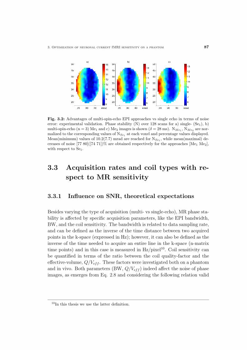
3. Optimization of neuronal current fMRI sensitivity on a phantom 87
Fig. 3.2: Advantages of multi-spin-echo EPI approaches vs single echo in terms of noiseerror: experimental validation. Phase stability (N) over 128 scans for a) single- (Se1), b)multi-spin-echo (n = 3) Me1 and c) Me2 images is shown (δ = 28 ms). NMe1 , NMe2 are nor-malized to the corresponding values of NSe1 at each voxel and percentage values displayed.Mean(minimum) values of 10.2(7.7) mrad are reached for NSe1 , while mean(maximal) de-creases of noise [77 80]([74 71])% are obtained respectively for the approaches [Me1 Me2],with respect to Se1.
3.3 Acquisition rates and coil types with re-
spect to MR sensitivity
3.3.1 Influence on SNR, theoretical expectations
Besides varying the type of acquisition (multi- vs single-echo), MR phase sta-
bility is affected by specific acquisition parameters, like the EPI bandwidth,
BW, and the coil sensitivity. The bandwidth is related to data sampling rate,
and can be defined as the inverse of the time distance between two acquired
points in the k-space (expressed in Hz); however, it can also be defined as the
inverse of the time needed to acquire an entire line in the k-space (n-matrix
time points) and in this case is measured in Hz/pixel10. Coil sensitivity can
be quantified in terms of the ratio between the coil quality-factor and the
effective-volume, Q/Veff . These factors were investigated both on a phantom
and in vivo. Both parameters (BW, Q/Veff ) indeed affect the noise of phase
images, as emerges from Eq. 2.8 and considering the following relation valid
10In this thesis we use the latter definition.
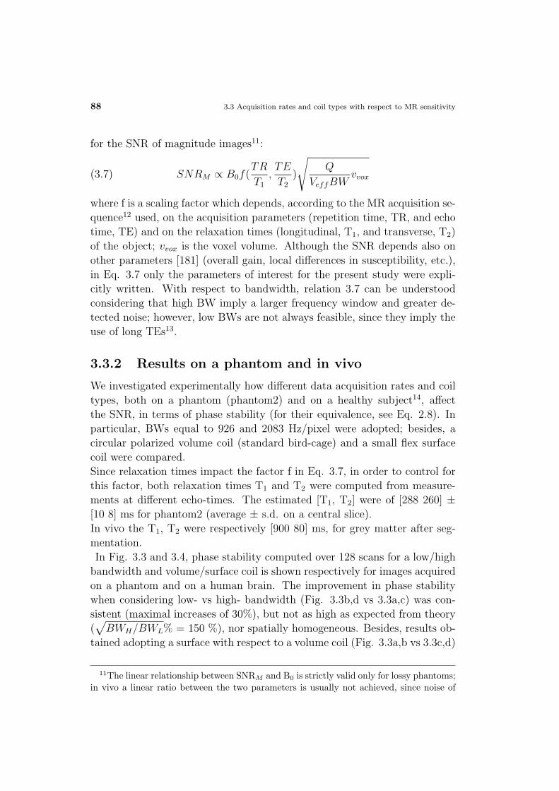
88 3.3 Acquisition rates and coil types with respect to MR sensitivity
for the SNR of magnitude images11:
(3.7) SNRM ∝ B0f(TR
T1
,TE
T2
)
√Q
VeffBWvvox
where f is a scaling factor which depends, according to the MR acquisition se-
quence12 used, on the acquisition parameters (repetition time, TR, and echo
time, TE) and on the relaxation times (longitudinal, T1, and transverse, T2)
of the object; vvox is the voxel volume. Although the SNR depends also on
other parameters [181] (overall gain, local differences in susceptibility, etc.),
in Eq. 3.7 only the parameters of interest for the present study were expli-
citly written. With respect to bandwidth, relation 3.7 can be understood
considering that high BW imply a larger frequency window and greater de-
tected noise; however, low BWs are not always feasible, since they imply the
use of long TEs13.
3.3.2 Results on a phantom and in vivo
We investigated experimentally how different data acquisition rates and coil
types, both on a phantom (phantom2) and on a healthy subject14, affect
the SNR, in terms of phase stability (for their equivalence, see Eq. 2.8). In
particular, BWs equal to 926 and 2083 Hz/pixel were adopted; besides, a
circular polarized volume coil (standard bird-cage) and a small flex surface
coil were compared.
Since relaxation times impact the factor f in Eq. 3.7, in order to control for
this factor, both relaxation times T1 and T2 were computed from measure-
ments at different echo-times. The estimated [T1, T2] were of [288 260] ±[10 8] ms for phantom2 (average ± s.d. on a central slice).
In vivo the T1, T2 were respectively [900 80] ms, for grey matter after seg-
mentation.
In Fig. 3.3 and 3.4, phase stability computed over 128 scans for a low/high
bandwidth and volume/surface coil is shown respectively for images acquired
on a phantom and on a human brain. The improvement in phase stability
when considering low- vs high- bandwidth (Fig. 3.3b,d vs 3.3a,c) was con-
sistent (maximal increases of 30%), but not as high as expected from theory
(√
BWH/BWL% = 150 %), nor spatially homogeneous. Besides, results ob-
tained adopting a surface with respect to a volume coil (Fig. 3.3a,b vs 3.3c,d)
11The linear relationship between SNRM and B0 is strictly valid only for lossy phantoms;in vivo a linear ratio between the two parameters is usually not achieved, since noise of
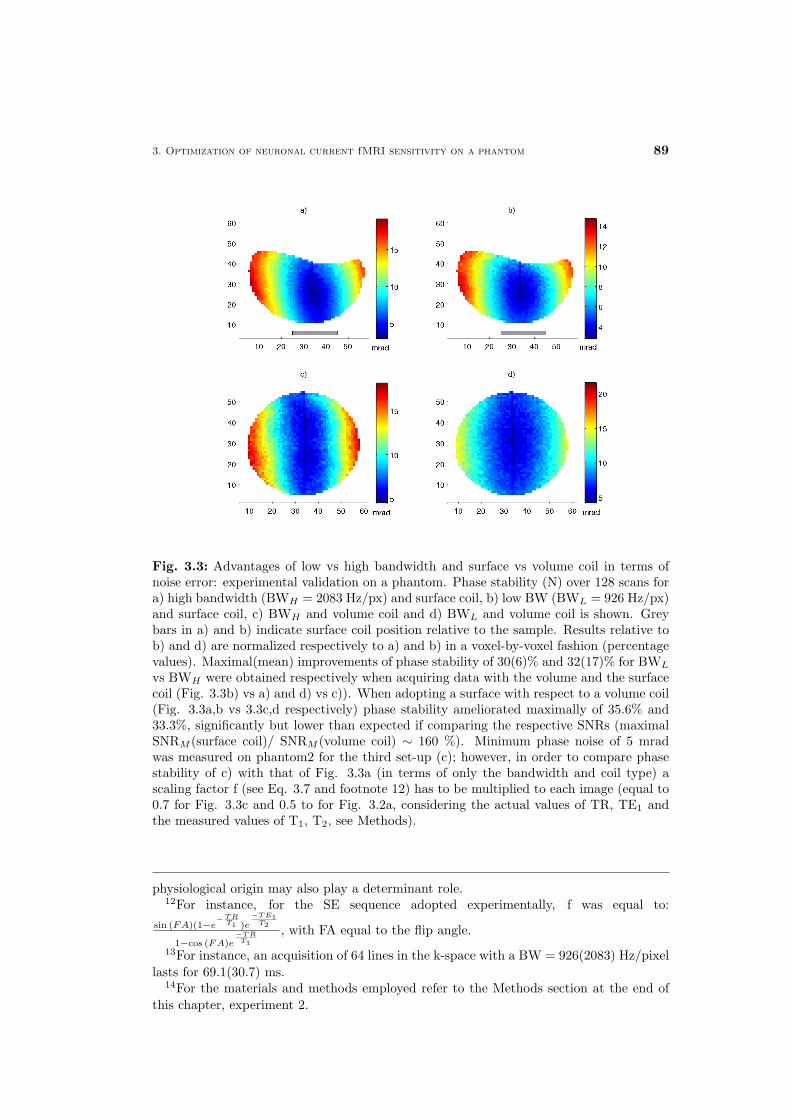
3. Optimization of neuronal current fMRI sensitivity on a phantom 89
Fig. 3.3: Advantages of low vs high bandwidth and surface vs volume coil in terms ofnoise error: experimental validation on a phantom. Phase stability (N) over 128 scans fora) high bandwidth (BWH = 2083 Hz/px) and surface coil, b) low BW (BWL = 926 Hz/px)and surface coil, c) BWH and volume coil and d) BWL and volume coil is shown. Greybars in a) and b) indicate surface coil position relative to the sample. Results relative tob) and d) are normalized respectively to a) and b) in a voxel-by-voxel fashion (percentagevalues). Maximal(mean) improvements of phase stability of 30(6)% and 32(17)% for BWL
vs BWH were obtained respectively when acquiring data with the volume and the surfacecoil (Fig. 3.3b) vs a) and d) vs c)). When adopting a surface with respect to a volume coil(Fig. 3.3a,b vs 3.3c,d respectively) phase stability ameliorated maximally of 35.6% and33.3%, significantly but lower than expected if comparing the respective SNRs (maximalSNRM (surface coil)/ SNRM (volume coil) ∼ 160 %). Minimum phase noise of 5 mradwas measured on phantom2 for the third set-up (c); however, in order to compare phasestability of c) with that of Fig. 3.3a (in terms of only the bandwidth and coil type) ascaling factor f (see Eq. 3.7 and footnote 12) has to be multiplied to each image (equal to0.7 for Fig. 3.3c and 0.5 to for Fig. 3.2a, considering the actual values of TR, TE1 andthe measured values of T1, T2, see Methods).
physiological origin may also play a determinant role.12For instance, for the SE sequence adopted experimentally, f was equal to:
sin (FA)(1−e−T R
T1 )e−T E1
T2
1−cos (FA)e−T R
T1
, with FA equal to the flip angle.
13For instance, an acquisition of 64 lines in the k-space with a BW = 926(2083) Hz/pixellasts for 69.1(30.7) ms.
14For the materials and methods employed refer to the Methods section at the end ofthis chapter, experiment 2.

90 3.4 Detection limit of current induced magnetic effects at 1.5 Tesla with optimized detection
Fig. 3.4: Advantages of low vs high bandwidth and surface vs volume coil in term ofnoise error: experimental validation in vivo on a human brain. Phase stability (N) over128 scans for a) high bandwidth (BWH = 2083 Hz/px) and volume coil, b) low bandwidth(BWL = 926 Hz/px) and surface coil is shown. Minimal noise values of 12.5 mrad for casea) and 8.6 mrad for b) were found. Here a scaling factor f of 0.3 (due to different T1, T2)has to be applied (multiplied) to compare these results with that in Fig. 3.2a (where f =0.5) or with Fig. 3.3b)-c) (f = 0.7).
ameliorated maximally of 35% and, most importantly if considering an in vivo
application, the noise feature showed mimimum values in the periphery of
the volume of interest rather than at the center. In vivo, the phase temporal
noise reached minimum values of about 8.6 mrad, when considering the best
hardware combination (BWL and surface coil, Fig. 3.4b), and of 12.5 mrad
in the worst case (BWH and volume coil, Fig. 3.4a). The maximum SNRM
was equal to 64 and 52, respectively in the former and in the latter case.
3.4 Detection limit of current induced mag-
netic effects at 1.5 Tesla with optimized
detection
In order to investigate the MR detection limit for weak magnetic field changes,
we induced electric currents in two parallel wires, immersed in a phantom
(phantom1) and positioned perpendicular to the external static magnetic
field B015. Phase changes were then measured for several current intensities.
In Fig. 3.5 activation maps, corresponding to different current intensities are
shown. The activation pattern agrees with the dipolar model, implemented
experimentally, with negatively correlated voxels in the space between the
15For the materials and methods employed refer to the Methods section at the end ofthis chapter, experiment 3.

3. Optimization of neuronal current fMRI sensitivity on a phantom 91
Fig. 3.5: MR detection limit of current induced phase changes at 1.5 Tesla: single-echoacquisition. Activation patterns in single-echo phase images corresponding to differentcurrent intensities, circulating in two parallel wires (see green arrows in the figure), inopposite directions, are shown. Current intensities equal to: a) 485.4, b) 106.4, c) 45.5,d) 22.7, e) 10.6, f) 8.9, g) 7.5 and h) 6.3 µA are employed; the correlation coefficientthreshold is equal to 0.11, which corresponds to a significance level p < 0.05, correctedfor 250 measurements). Phase changes induced by current intensities as low as 10.6 and8.9 µA are still detectable by a 1.5 Tesla MR system. The black arrow indicates the pixelwith the minimum detectable phase change (CNR = 22 %).
wires and correlations of opposite sign occurring outside. It emerges clearly
that phase changes induced by current intensities as low as 10.6 and 8.9
µA are still detectable by a 1.5 Tesla MR system. In particular, with an
underlying noise of 6.8 mrad (close to that achieved in vivo with the best
experimental conditions), 8.9 µA current induced phase changes of 1.5 mrad
were detectable at 1.5 Tesla (Fig. 3.5, pixel indicated by a black arrow), when
considering a single-echo acquisition16. In order to scrutinize further this re-
sult, we report the phase time-series extracted for each current intensity in
16For magnitude images, activation maps were not visible for currents lower than 50 µA;for higher current intensities the extension of the activation patterns was considerablyrestricted with respect to that in the corresponding phase images, comprising only fewvoxels around the wires positions.
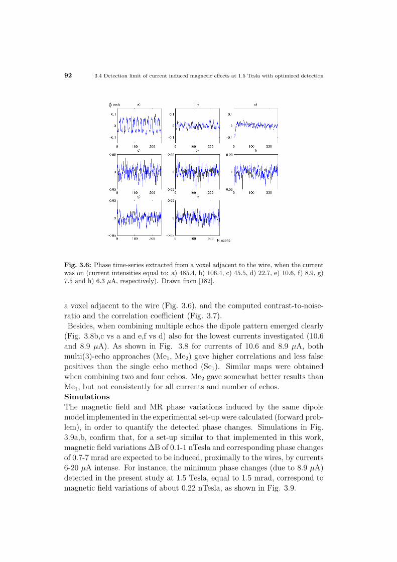
92 3.4 Detection limit of current induced magnetic effects at 1.5 Tesla with optimized detection
Fig. 3.6: Phase time-series extracted from a voxel adjacent to the wire, when the currentwas on (current intensities equal to: a) 485.4, b) 106.4, c) 45.5, d) 22.7, e) 10.6, f) 8.9, g)7.5 and h) 6.3 µA, respectively). Drawn from [182].
a voxel adjacent to the wire (Fig. 3.6), and the computed contrast-to-noise-
ratio and the correlation coefficient (Fig. 3.7).
Besides, when combining multiple echos the dipole pattern emerged clearly
(Fig. 3.8b,c vs a and e,f vs d) also for the lowest currents investigated (10.6
and 8.9 µA). As shown in Fig. 3.8 for currents of 10.6 and 8.9 µA, both
multi(3)-echo approaches (Me1, Me2) gave higher correlations and less false
positives than the single echo method (Se1). Similar maps were obtained
when combining two and four echos. Me2 gave somewhat better results than
Me1, but not consistently for all currents and number of echos.
Simulations
The magnetic field and MR phase variations induced by the same dipole
model implemented in the experimental set-up were calculated (forward prob-
lem), in order to quantify the detected phase changes. Simulations in Fig.
3.9a,b, confirm that, for a set-up similar to that implemented in this work,
magnetic field variations ∆B of 0.1-1 nTesla and corresponding phase changes
of 0.7-7 mrad are expected to be induced, proximally to the wires, by currents
6-20 µA intense. For instance, the minimum phase changes (due to 8.9 µA)
detected in the present study at 1.5 Tesla, equal to 1.5 mrad, correspond to
magnetic field variations of about 0.22 nTesla, as shown in Fig. 3.9.
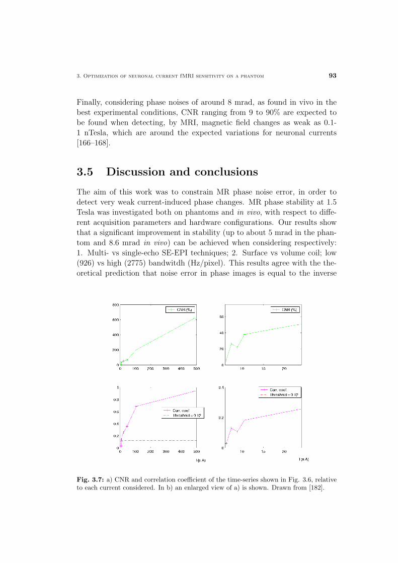
3. Optimization of neuronal current fMRI sensitivity on a phantom 93
Finally, considering phase noises of around 8 mrad, as found in vivo in the
best experimental conditions, CNR ranging from 9 to 90% are expected to
be found when detecting, by MRI, magnetic field changes as weak as 0.1-
1 nTesla, which are around the expected variations for neuronal currents
[166–168].
3.5 Discussion and conclusions
The aim of this work was to constrain MR phase noise error, in order to
detect very weak current-induced phase changes. MR phase stability at 1.5
Tesla was investigated both on phantoms and in vivo, with respect to diffe-
rent acquisition parameters and hardware configurations. Our results show
that a significant improvement in stability (up to about 5 mrad in the phan-
tom and 8.6 mrad in vivo) can be achieved when considering respectively:
1. Multi- vs single-echo SE-EPI techniques; 2. Surface vs volume coil; low
(926) vs high (2775) bandwitdh (Hz/pixel). This results agree with the the-
oretical prediction that noise error in phase images is equal to the inverse
Fig. 3.7: a) CNR and correlation coefficient of the time-series shown in Fig. 3.6, relativeto each current considered. In b) an enlarged view of a) is shown. Drawn from [182].

94 3.5 Discussion and conclusions
of the signal-to-noise-ratio of magnitude images (Eq. 2.8) [133]. With re-
spect to multi-echo approaches, their implementation is simpler for samples
with long T2 (e.g. at low static magnetic fields), being concurrently longer
the inter-echo spacing for which their advantage vs single-echo acquisition is
demonstrated. For short T2, special acquisition strategies, like partial sam-
pling of k-space, or the use of faster gradients, may be needed. With respect
to the coil type, its quality-factor/effective-volume may not be an exhaustive
parameter for noise characterization over time, since pulse stability could
affect differently the two coil performances (assumed equal in this work).
Beside we showed that, when inducing a current of 8.9 µA (duration 25 ms)
in two parallel wires in opposite directions, the minimum detectable phase
variations are of 1.5 mrad (corresponding to magnetic field variations of 0.22
nTesla), with an underlying phase noise of about 6.8 mrad; besides, when
combining multiple echos the dipolar pattern emerges clearly also for the
Fig. 3.8: MR detection limit of current induced phase changes at 1.5 Tesla: multi-echoacquisition. Activation patterns in single-(a,d) and multi- (Me1, b-e, Me2, c-f) echo phaseimages for current intensities equal to 10.6 (a,b,c) and 8.9 (d,e,f), circulating in two parallelwires (see green arrows in the figure), in opposite directions, are shown. Threshold is setas in Fig. 3.5. Minimum phase changes of 2 and 1.5 mrad induced respectively by currentintensities as low as 10.6 and 8.9 µA, in pixels indicated by the black arrows, were stilldetectable by a 1.5 Tesla MR system, using multi-echo approaches. In particular the CNRincreased from 19(14)% to 24(23)% when applying multi-echo approaches (Me1, Me2) vssingle ones (respectively for 10.6 and 8.9 µA).

3. Optimization of neuronal current fMRI sensitivity on a phantom 95
lowest currents investigated (10.6 and 8.9 µA). These results are encourag-
ing for in vivo imaging, since magnetic field variations induced by neuronal
currents are expected to range between tenth of nTesla to few nTesla [166–
168]; for instance 0.1-1nTesla variations correspond to phase changes of 0.7-7
mrad, for our experimental set-up (see simulations). Our result is close to
previous findings at 3 Tesla [166–168], obtained by a higher (four times or
more) number of scans and with different choices for the TR, TE and other
parameters. It demonstrates that optimized acquisition and post-processing
methods rather than a high static magnetic field strength are crucial to de-
tect small changes in MR phase images. In the next chapter, in order to
generalize our findings, valid for the optimization of phase noise, we also
discuss the effects of acquisition parameters and of other factors on the MR
contrast.
In conclusion, multi-echo spin-echo approaches seem promising in order to
improve the detection sensitivity for small phase changes, as well optimiza-
tion of acquisition parameters and hardware configuration. These results
are encouraging for in vivo MR phase imaging of neuronal current effects,
although the feasibility of such a functional approach relies on a good spatio-
Fig. 3.9: Simulations of a dipole model similar to the one implemented experimentally(wires distance ' 10 pixels). a) Magnetic field (nTesla) and b) MR phase variations (rad)induced by the same dipole model implemented in the experimental set-up.
96 Materials and methods
temporal synchronization between MR acquisition and the electric event. For
instance, in case of evoked electric cerebral components, the use of single-
and, whenever possible, of multi-spin-echo images may enhance the contrast
due to successive components of opposite sign. These issues are dealt in de-
tail in the following chapter.
Materials and Methods
Phantoms and participantsTwo phantoms (phantom1, phantom2) containing water doped with CuSO4
(see below, for their measured T1 and T2) were employed for measurement
of noise stability.
One healthy subject (female, 26 yr) volunteered to participate in the study
and gave informed consent according to guidelines reviewed and approved by
local ethics authorities for work involving humans. The participant had to
lay supine inside the magnet bore throughout the experiment, without any ex-
ternal stimulation. Positioning was performed so that the participant’s head
would be approximately centred in the standing magnetic field of the MR and
head movement was minimised by mild restraint and cushioning.
ApparatusA Siemens Vision Magnetom MR system (Siemens Medical Systems, Erlan-
gen, Germany) operating at 1.5 Tesla and equipped for echo-planar imaging
was employed for acquiring MR images. Two head coils were used for radio
frequency transmission and reception: a circular polarized volume head coil
(standard birdcage) and a small flex surface coil (37 cm wide, 17 cm high),
optimized for brain imaging. Image analyses were performed on software
(see “Image processing”) running on LINUX (Debian 3.0), on a IBM server
(xSeries 235, Intel Xeon 2.4 GHz dual processor).
MRI data acquisitionT1, T2 measurements: Relaxation parameters (T1, T2) were measured
for the phantoms and in vivo. For both phantoms, a multi echo spin-echo
sequence (FA = 90o/180o, TE = [70 120 170 230 280 380 480] ms, TR =
[3.4 4.46 5.51 6.77 7.82 9.92 12.02] ms) and an inversion recovery-spin-echo
sequence (FA = 180o/90o/180o, TI = [60 100 150 200 300 600 1200] ms, TE
= 70 ms, TR = [24.6 25.4 26.4 27.4 29.4 35.4 47.4] s) were used. Other
parameters common to both sequences were: N. slices = 20, slice thickness =
5 mm, field of view (FOV) = 240 mm, matrix = 128 × 128. In vivo, a multi
spin-echo sequence (16 echos, TE = [50 50 + δ 50 + 2δ ... 50 + 15δ], d =
50 ms, TR = 2.20 s, 1 slice) and an inversion recovery-spin-echo sequence

Optimization of neuronal current fMRI sensitivity on a phantom 97
(TI = [50 100 150 200 300 500 750 1000 1500 2000 3500 5000] ms, TE = 70
ms, TR = [24.4 25.4 26.4 27.4 29.4 33.4 38.4 43.4 53.4 63.4 93.4 123.4] s, 4
slices) were used. Nonlinear regression (Levenberg-Marquardt with gradient-
descent to increase convergence speed) was performed to fit the experimental
data to the T1 and T2 decay curves obtained from the Bloch equations thus
voxel-wise estimates of the relaxation times, T1 and T2, were obtained.
Experiment 1 - Phase stability on a phantom, multi- vs single-
echo SE-EPI techniques: Single- and multi-spin-echo EPI magnitude and
phase images of phantom1 were acquired using a volume coil with the follow-
ing parameters: FA = 90o/180o, TR = 3 s, TE1 = 60 ms, TE2 = TE1 +
d, TE3 = TE1 + 2*d, TE4 = TE1 + 3*d, inter-echo spacing (δ) = 28 and
45.4 ms (in two different sessions), BW = 2083 Hz/pixel, N. slices = 3,
slice thickness = 5 mm, slice orientation: coronal, FOV = 192 mm, matrix
= 64 x 64, 128 scans. In order to shorten the inter-echo delay to 28 ms,
only the central 32 lines of k-space were sampled in the phase-encoding di-
rection. During post-processing, the remaining 32 lines were zero-filled and
a 2D-Gaussian filter (Full width half maximum, FWHM = 26.6 points) was
applied previous to Fourier Transform. For d = 45.4 ms, full k-space sam-
pling was performed. Phase stability was computed on both single- (Se1) and
multi-echo (Me1, Me2) images (for a number of echos n = 2, 3 and 4, re-
spectively), as described below (see “MRI data processing”), and results for
the different approaches were compared.
Experiment 2 - Phase stability on a phantom and in vivo, coil
type and bandwidth (BW) influence: Single-spin-echo transversal EPI
phase images of phantom2 were acquired with the following parameters: FA
= 88o/180o, TR = 1 s, TE1 = 83.08 ms, N. slices = 3, slice thickness =
5 mm, FOV = 192 mm, matrix = 64 × 64, full-k-space 2D-transformed,
129 scans. Four sessions were run, with two different coil types (volume
and suface) and bandwidths (BWL = 926 and BWH = 2083 Hz/pixel). The
measurement was repeated for the healthy subject with the same acquisition
parameters (except for the slice orientation, coronal, for the FA = 70o/180o
and N. scans = 134), for two different hardware configurations (volume coil
and high bandwidth; surface coil and low bandwidth). The first images (1 for
the phantom and 6 in vivo) were discarded from further analysis to remove
any possible T1 saturation effects. Phase image stability (s.d. over 128 scans
for each voxel, in mrad) was computed for each session, after pre-processing,
as explained below (see “MRI data processing”) and results for the different
configurations compared.
Experiment 3 - Detection limit of current-induced phase changes

98 Materials and methods
inside a phantom at 1.5 Tesla: A rectangular closed electric circuit, per-
pendicular to the static magnetic field, was immersed in the solution of phan-
tom1. At specific time points, electric currents (intensities: 485.4, 106.4,
45.5, 22.7, 10.6, 8.9, 7.5 and 6.3 µA; duration: 25 ms) were induced in the
circuit with a 10 scans ON/OFF cycle. For each current intensity inves-
tigated, coronal single spin-echo EPI phase images were measured with the
same hardware configuration and acquisition parameters as in Experiment 1,
except for the number of scans that now were doubled to 256, due to alter-
nating of “resting” and “active” measurements. For currents with intensities
of 10.6 and 8.9 mA, multi-echo images (see Experiment 1 for acquisition pa-
rameters) were acquired at two different experimental sessions. The first six
images were discarded from further analysis to remove any possible T1 satu-
ration effects. A National Instruments (Austin, Tx) board triggered, with 1
kHz precision, the start of both the MRI acquisition and the electric currents
to assure the occurrence of the electric event between the first two MR-pulses
(i.e. 90o/180o, see Fig. 3.1a). Each phase image was processed as described
below (see “MRI data processing”) and activation maps were obtained for
each current intensity applied.
MRI data processingFor each Experiment, image pre-processing was performed with software de-
veloped in Matlab, version 6.0 (The MathWorks, Inc., Natick, MA): each
phase time-series inside the object (obtained after image masking, see below)
was time unwrapped and then linearly detrended. For phantom images, voxels
were removed if signal in the corresponding magnitude voxels was lower than
60(20)% of each slice maximum value respectively for volume(surface) coil
images. In vivo, masking was performed with a threshold of 30(20)% of each
slice maximum value respectively for volume(surface) coil images. For mag-
nitude images only linear detrending and masking were applied. Multi-echo
images were combined by two approaches (see Par. 3.2.1, Eq. 3.1b,c): 1)
simple sum (Me1); 2) weighted sum (Me2), with weighting factors, for each
echo, proportional to the noise standard deviation of each voxel time-series
during the run, for Experiment 1 and 2, and during the current OFF periods
only, for Experiment 3. For each voxel of both single- (Se) and multi-echo
(Me1, Me2) images, phase stability (expressed in mrad) was obtained by com-
puting the s.d. over all the scans in a run, for Experiment 1 and 2, and over
the scans during the current OFF periods for Experiment 3. SNRM of magni-
tude images was computed as the fraction of the mean value divided by the s.d.
over time during resting periods. For Experiment 3, both single- (SE) and
multi-echo (ME1, ME2) images were statistically analyzed by the Analysis of
Optimization of neuronal current fMRI sensitivity on a phantom 99
Functional NeuroImages tool (AFNI 2.55f): correlation coefficients between
phase time-series and a boxcar regressor reflecting the ON/OFF cycle were
calculated, after high-pass filtering that removed the phase signal offset and
its linear drift. Activation maps were thresholded at r = 0.11, corresponding
to a significance level of p < 0.05 for 250 scans (uncorrected).
Simulations: For a dipolar model (wires distant each other 10 pixels)
comparable to the one implemented in the experimental set-up (Experiment
3.), both induced magnetic field and MR phase variations were computed by
applying respectively the Laplace law in Eq. 2.15, which reduces to the Biot-
Savart low, for a plane orthogonal to two ideal and parallel conducting-wire
(rectilinear and infinitely long) and Eq. 2.5 (assuming a point-shaped voxel).

Chapter 4
Neuronal current fMRI of in
vivo visual evoked activity
In the previous Chapter, we showed that MRI has enough sensitivity to detect
small magnetic field variations (0.1-0.2 nTesla) along the external magnetic
field, induced by applying currents in electric circuits positioned inside water
phantoms. These results were found both at 3 Tesla [167, 168] and at 1.5
Tesla [169] and demonstrated that expected neuronal currents field distor-
tions may be detected by MRI. Despite these encouraging results, some issues
are still of intense debate, such as optimization of the acquisition strategy
for detection of neuronal magnetic effects and the practicability of detecting
them in vivo.
In this chapter, we first describe how optimization of the neuronal current
contrast may be achieved. Any gain in MR sensitivity would be useful in
order to detect neuronal-current induced signal changes, since they are ex-
pected to be modest [166–168] with respect to the intrinsic noise. MR sen-
sitivity may be increased either by decreasing the noise, as shown in the
previous chapter, or by increasing the signal change itself. Improvement of
the expected signal changes may be obtained by several means, for instance
by prolonging the duration and strength of the neuronal event, by optimiza-
tion of the geometrical characteristics of the current dipole with respect to
the externally applied magnetic field and image voxel localization, and by
an accurate synchronization between the neuronal event and the MR acqui-
sition [168, 173]. These solutions will be evident from relations governing
the current-induced contrast-to-noise-ratio (CNR) for a single voxel in a MR
image, which are elucidated in Par. 4.1.
We then compare previous findings regarding both spontaneous activity and
101

102 4.1 Neuronal current fMRI contrast optimization
evoked responses and outline the limiting experimental factors for the detec-
tion of these two facets of brain electrical response, see Par. 4.2.
Then we motivate our stimulation and acquisition choices and we describe
two approaches: the first, to spatio-temporal synchronize the electric event
with the MR acquisition and, the second, to control possible artifacts (Par.
4.3).
Finally, we report on our pilot study, which regards the feasibility to detect,
for the first time, magnetic field effects caused by neuronal activity in vivo
by spin-echo MR imaging (MRI), see Par. 4.4.
Parts of the results shown in this chapter were published in [173].
4.1 Neuronal current fMRI contrast optimiza-
tion
In order to detect neuronal-current effects by MRI, together with noise reduc-
tion by optimized acquisition and post-processing, as shown in the previous
chapter, phase contrast in spin-echo EPI images should be maximized too.
The CNR for a single voxel in a phase or magnitude image is governed by
Eq. 2.9. With respect to the modulations of several acquisition parameters
on the SNRM or equivalently on the phase noise we refer to Par. 3.3.1. Here,
we disentangle which factors play a role for detecting current-induced signal
changes in both the MR magnitude and phase; at this purpose, we rewrite
more explicitly relations for the terms ∆Φ and ∆M/M0 with the help of Eq.
2.5, as follows:
(4.1)
∆Φ = CΦ = arg(
∑k ei∆ΦJ
k (r(t)))∆MM0
=∑
k cos(∆ΦJk −∆Φ)− 1.
∆ΦJk (r(t)), considering a SE acquisition and Eq. 2.61, is equal to:
(4.2) ∆ΦJk (r(t)) = 2πγ
∫ TE/2
0
∆BJk (r, t′)‖dt′ −
∫ TE
TE/2
∆BJk (r, t′)‖dt′)
∆BJk‖ is the total component of the induced magnetic field by the current
density J, parallel to the B0.
1∆ΦJk stands for Φk
tis of Eq. 2.6, with ∆ and J referring explicitly to the current Jinduced phase variations (with respect to the phase for J = 0).
4. Neuronal current fMRI of in vivo visual evoked activity 103
From relations 4.1 and 4.2 and from those explicated in Par. 2.5 (Eq. 2.15-
2.18), it can be evinced that the contrast depends, on one hand, on some
acquisition parameters: for instance, the echo-time, the voxel size, the trig-
gering with the electric event, the slice orientation with respect to the dipole,
but not the B0 strength. On the other hand, it relies on the intrinsic electric
phenomenon: e.g. the dipolar temporal duration, intensity and orientation
with respect to B0.
For some parameters, such as the echo-time, a trade off between high con-
trast and low noise in neuronal-current spin-echo MR phase images has to
be met: for long duration (100 - 200 ms as found for evoked potentials) of
the neuronal event, long TEs are valuable in terms of high contrast, but in-
adequate for constraining phase noise, see Eq. 3.7 (this effect getting worse
the higher the field strength); equivalently with respect to varying the voxel
dimensions, the higher the voxel volume, the lower the phase error [168], but
concurrently the lower the contrast of phase images due to partial volume
effects. Other parameters, such as the magnetic field strength, doesn’t in-
fluence the contrast in neuronal-current MRI, but only the noise figure (Eq.
2.8).
The other requisites for optimizing the contrast need the knowledge of bio-
currents spatio-temporal characteristics, which can potentially be drawn by
other measurements (EEG-MEG): so as duration and latency with respect
to stimulus onset, to synchronize the MR images acquisition with the elec-
tric event, which is particularly crucial for SE measurements in order to not
refocus the dipolar effect during acquisition; as well as the knowledge of the
orientation dipole, in order to orient the dipole, as much as possible, orthog-
onal to the external static magnetic field, and concurrently to acquire the
slices in a direction orthogonal to the current-dipole axis, in order to obtain
a dipolar pattern. At this aim, we propose the combined use of visual evoked
potential (VEP) recordings and BOLD-fMRI measurements prior to neuronal
current MRI-scanning. Before reporting on the proposed approach and on
results of a pilot study, relative to its application, we discuss in the next
paragraph about the feasibility of neuronal current fMRI in vivo. Previous
findings and the rationale behind our study are treated together, outlining
the main limitations and possible solutions with regard to the investigation
of different type of neuronal activity.

104 4.2 In vivo feasibility of neuronal current fMRI
4.2 In vivo feasibility of neuronal current fMRI
4.2.1 Spontaneous versus evoked activity
Recent works have investigated the feasibility to detect primary magnetic
effects induced by neuronal currents during brain activity by MRI [171,
174, 194–196]. Discordant results were found with regard to the MRI detec-
tion of both neuronal spontaneous activity [194, 195] and evoked responses
[171, 174, 196], the two facets of cerebral activity mostly studied by EEG-
MEG methodologies.
For instance, Xiong et al. [171] and Chu et al. [174] reported opposite find-
ings with respect to the detection of evoked responses. The first found con-
sistently for six subject a stimulus evoked response in visual and motor areas
detected by the “magnetic-source” MRI technique. Their paradigm consisted
in a 1 ON/OFF scan stimulus cycle2 and of a sliding window acquisition of
each slice with respect to the stimulus onset in different experimental runs.
On the contrary Chu et al. [174], in eight volunteers, did not detect any rapid
MRI signal changes during visual-evoked response3. They used m-sequences
for the stimulation design, which enables discrimination between fast (pro-
bably neuronal) and low (hemodynamic) responses. Differently, Kilner et al.
[196] studied the steady state (see pag. 20) evoked neuronal response to a
10 Hz flickering visual stimulus in three subjects and found significant com-
ponents at this rate in both the amplitude and the phase of the MR signal4.
The investigation of spontaneous activity was performed by Liston et al.
[195] for generalized 3 Hz spike-wave discharges in epileptic patients and by
Leach et al. [194] for alpha wave activity. In the investigated patient, Liston
et al. demonstrated a significant MRI activity at a time scale of the order of
30 ms, but concluded that further work is necessary before firm conclusions
2For such a high frequency design, discrimination between neuronal current effects andthe BOLD response is achieved, since the latter is saturated. However, actually the authorsdetected neuronal current evoked responses at exactly the Nyquist frequency, which mayimply the loss of some power. They acquired 5 slices (TR = 1 s, TE = 100 ms, GEEPI sequence), in 5 distinct runs, each with a different slice timing with respect to thestimulation onset.
3They acquired only one slice, due to the short employed TR (100ms); however theSNR was boosted by the use of a 3 T and a 16-channel coil. Two different delays wereemployed, with respect to stimulation timing, equal to 0 and 50 ms, respectively.
4Volumes constituted of ten contiguous slices were acquired with a TR = 100 ms (TE= 50 ms) and a 40 ms delay between consecutive volumes in order to jitter image samplingwith respect to the stimuli.
4. Neuronal current fMRI of in vivo visual evoked activity 105
may be drawn5. Similar claims for the other cited work, since Leach et al.
could observe a statistically significant correlation between the power mod-
ulation of EEG and MR phase in the alpha frequency band for four of five
investigated subjects6; however there was large intra-subject variation be-
tween trials for each subject and on the authors’ opinion the observed effects
require further investigation, being the interpretation of their finding also
limited by the uncertain nature of the electric generator, underlying alpha
waves7. Finally, in in vitro tissue cultures, Petridou et al. [170] succeeded
in detecting spontaneous synchronized activity (0.15 Hz) in spin echo phase
images8.
Although spontaneous rhythms have greater amplitudes, evoked responses
have two main advantages: first, they have a precise latency with respect to
the event, measurable by EEG-MEG; second, they can be better localized,
by EEG-MEG and BOLD fMRI. Both features together enable the use of
repetition times close to that commonly used in BOLD fMRI (∼s), without
compromising the SNR9; hence the detection of more than one slice posi-
tioned in the locus of activation can be achieved. Finally evoked responses
are better localized than spontaneous or epileptic activity. The benefit for
the investigation of specific cases of evoked, spontaneous and paroxismal ac-
tivity in terms of the achievable MR contrast, noise and CNR is described
qualitatively in Fig. 4.1.
For all these reasons, we started with investigating evoked responses 10,
elicited in visual areas, and we proposed solutions for synchronization and
contrast optimization, which are described in Par. 4.3.
5Volumes of 21 slices were acquired with a TR = 3 s and a TE = 40 ms (GE sequence);four 3 Hz spike-wave discharges occurred in the investigated patient, during a 35 min ofEEG-correlated fMRI acquisition.
6Simultaneous EEG and fMRI recordings were performed; relative to the MR acquisi-tion (GE sequence), a TR = 40 ms and a TE = 24 ms were employed and one slice foreach subject was investigated.
7The works [170, 196] were presented only in abstract form at conferences, while resultspresented in abstracts [194, 195] were recently fully published, see [199, 200].
8Phase images of four slices were acquired for about 20 min (TR = 1 s, TE = 60 ms).9Detecting for instance a 3 Hz wave requires at least a repetition time of 166 ms, a 10
Hz a TR of 50 ms; such low TR deteriorate the SNR, see Eq. 3.7 and footnote 12 of Chap.3. Besides, in this case, only one slice per experimental run can be acquired.
10The study of epileptic discharges is a work in progress and is not dealt in detail inthis thesis.
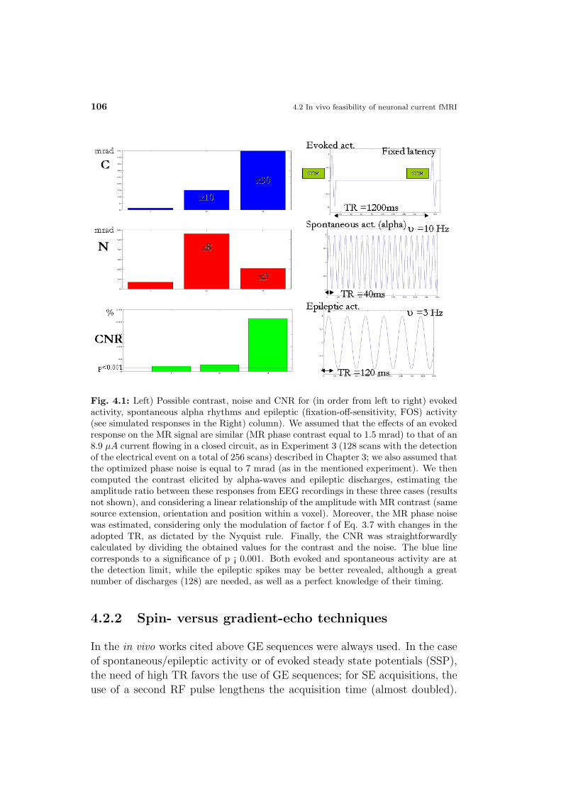
106 4.2 In vivo feasibility of neuronal current fMRI
Fig. 4.1: Left) Possible contrast, noise and CNR for (in order from left to right) evokedactivity, spontaneous alpha rhythms and epileptic (fixation-off-sensitivity, FOS) activity(see simulated responses in the Right) column). We assumed that the effects of an evokedresponse on the MR signal are similar (MR phase contrast equal to 1.5 mrad) to that of an8.9 µA current flowing in a closed circuit, as in Experiment 3 (128 scans with the detectionof the electrical event on a total of 256 scans) described in Chapter 3; we also assumed thatthe optimized phase noise is equal to 7 mrad (as in the mentioned experiment). We thencomputed the contrast elicited by alpha-waves and epileptic discharges, estimating theamplitude ratio between these responses from EEG recordings in these three cases (resultsnot shown), and considering a linear relationship of the amplitude with MR contrast (samesource extension, orientation and position within a voxel). Moreover, the MR phase noisewas estimated, considering only the modulation of factor f of Eq. 3.7 with changes in theadopted TR, as dictated by the Nyquist rule. Finally, the CNR was straightforwardlycalculated by dividing the obtained values for the contrast and the noise. The blue linecorresponds to a significance of p ¡ 0.001. Both evoked and spontaneous activity are atthe detection limit, while the epileptic spikes may be better revealed, although a greatnumber of discharges (128) are needed, as well as a perfect knowledge of their timing.
4.2.2 Spin- versus gradient-echo techniques
In the in vivo works cited above GE sequences were always used. In the case
of spontaneous/epileptic activity or of evoked steady state potentials (SSP),
the need of high TR favors the use of GE sequences; for SE acquisitions, the
use of a second RF pulse lengthens the acquisition time (almost doubled).

4. Neuronal current fMRI of in vivo visual evoked activity 107
However, for evoked responses, with a defined latency with respect to stimu-
lus onset and duration, a good temporal synchronization would enable the
use of both GE and SE sequences.
The choice of the acquisition sequence (GE or SE) will undoubtedly impact
the outcome of neuronal current MR measurements. There are several advan-
tages associated with the SE technique for the detection of evoked responses.
First, non-neuronal contributions to the signal which are slower than the
echo time, such as movement-related artifacts and other physiological (e.g.
BOLD) static contributions to the signal, are refocused and hence minimized
with respect to a GE acquisition. A better discrimination between fast and
slow processes accomplished by SE with respect to GE techniques was indeed
reported in [167] for currents flowing in a circuit. This may also be useful
to delete contributions of possible spontaneous activity (>(2*TE)−1 Hz11)
during evoked responses, which are at least an order of magnitude greater
than the former, but that, however, are not stimulus phase-locked.
Second, BOLD effect sizes in SE magnitude images are lower than in GE
images due to the distinct averaging phenomena (dynamic versus static),
as described in Par. 2.3; moreover, at high fields (> 3 Tesla), but only for
SE sequences, the macro-vascular contribution to the signal is suppressed
[155, 156], while at low fields (1.5-3 Tesla) intra-vascular dephasing effects
are still present and constitute the dominant contribution to the signal [183],
see Par. 2.3.
Third, if both positive and negative components are present in the evoked
response, a SE acquisition may be synchronized in order to sum both the
contributions (for example positioning in time one component in the first
half of the echo time and the other, of opposite sign, in the second half).
This was achieved in vivo in our study, see for instance Fig. 4.8a.
Conversely, the main advantages with GE acquisitions is that there is no
risk of refocusing the effect of the neuronal currents; besides, as said above,
this technique is more suited when high scanning rates are needed, e.g. for
the detection of oscillating signal components (steady state evoked responses
or spontaneous/epileptic activity) and/or when the latency of the response,
with respect to the stimulus is unpredictable. On the contrary, in SE mea-
surements only, symmetric time evolution of the neuronal event around the
refocusing pulse must be avoided. At this aim, long echo times (TE = 100
- 200 ms) are generally needed to accommodate the time evolution of the
11For instance, for a SE acquisition with TE = 100 ms, waves of frequency ≥ 5 Hz arerefocused.
108 4.3 Overview of the proposed approaches
neuronal currents, as will be shown in the present work.
In conclusion, on our opinion, SE techniques are more suitable than gradient-
echo GE strategies for detecting evoked primary effects of neuronal currents.
For this reason, SE strategies were adopted in the present work.
In the following paragraph we overview the approach adopted in the present
work to detect neuronal currents.
4.3 Overview of the proposed approaches
In vivo, discrimination between primary neuronal effects and secondary
hemodynamic-metabolic changes is fundamental for a successful application
of neuronal current MRI. In order to minimize any ambiguity in this respect,
we preferred the use of SE acquisition for our in vivo work on a healthy sub-
ject. In order to maximize SE image contrast, we developed methods that
enable an exact temporal synchronization of the neuronal event with the MR
SE acquisition. In order to gain knowledge of the temporal dynamics of the
neuronal events, EEG-recordings of visual evoked potentials (VEP) were per-
formed for the subject under investigation: the same stimulus as for MRI was
used. The SE sequence subsequently adapted to reflect the dynamics of the
dipolar sources and information regarding the dipolar geometry estimated by
EEG recordings was used for positioning of the subject and the measurement
slices during the MR experiments. This approach was motivated by the fact
that only magnetic field variations parallel with the external magnetic field
B0 can be detected, and hence the orientation of the dipole, in particular
its orthogonality with respect to B0, is crucial. During the course of the
MR examination, besides neuronal current SE MRI, conventional BOLD GE
and SE fMRI were also performed. For a detailed description of the spatio-
temporal synchronization between the electric event and the MR acquisition,
see Par. 4.3.1.
We also outline some theoretical considerations regarding the experimen-
tal design used for neuronal current SE MRI, and show how this can help in
further optimizing measurements, assessing the possibility to control for arte-
factual signal changes due to BOLD and movement effects, see Par. 4.3.2.
Finally, we report on a pilot study using the proposed combination of EEG
and MRI techniques, see Par. 4.4.

4. Neuronal current fMRI of in vivo visual evoked activity 109
4.3.1 The VEP-fMRI approach for synchronizing the
neuronal event with SE MR measurements
Synchronization of spin-echo MR images with the neuronal event, which is
the basis for an optimal SE-MRI contrast, relies on the knowledge of spe-
cific features of the brain response: for instance, dipole time evolution and
orientation, in a given subject and for a specific stimulation employed in the
neuronal current MRI measurement. At this aim, we introduce a method
which combines information from EEG recordings of visual evoked poten-
tials (VEP) and fMRI measurements, performed separately but on the same
subject and using the same stimuli. It consists of the following steps:
Prior to MRI scanning:
1. Characterization of the dipolar source. High resolution (64 channels)
VEP recording and estimation of the location, orientation and signal
dynamics (onset, peak, duration and sign of the signal) of the dipolar-
sources (equivalent current dipoles, ECDs) subtending the first major
VEP component (C1)12.
During MRI scanning:
2. Adaptation of the SE MRI sequence. Echo time (TE) and stimulus
timing with respect to SE MRI acquisition are adapted to reflect the
dipolar time evolution, see Fig. 4.2a.
3. Adaptation of MRI acquisition to the geometry of the dipolar source.
Optimization of patient positioning within the bore of the MR scanner
in order to achieve orthogonality between dipolar orientation and static
magnetic field, as far as possible (Fig. 4.3). In this respect, specific
visual stimuli (Fig. 4.2b) known to generate dipolar sources with minor
components along the static magnetic field, after subject positioning
12See “ERP analysis” in the Methods section for details. In brief, the signal dynamicscan be extracted by repeated averaging of EEG traces in phase with the stimulus delivery;the dipole orientation and localization by the solution of the inverse problem, by iterativecomparison of the estimated (solution of the forward problem) and measured potentialstopography, once assumed a model. See Fig. 4.8, for a realistic example of the measuredand the estimated potential topography on one investigated subject.

110 4.3 Overview of the proposed approaches
inside the MR-scanner, can be chosen. In addition, the measurement
slices are oriented orthogonal to the VEP dipole and are positioned so
that both VEP-source and active BOLD regions are covered (Fig. 4.3).
Fig. 4.2: Temporal synchronization of MRI acquisition and stimulus delivery. The tim-ing of the visual stimulus was made to optimize the dipolar time evolution during MRexcitation and refocusing. As shown in a), RF pulses were temporally positioned and theecho time was adapted in order to avoid refocusing of the dephasing event determined byVEP. For instance, the time-evolution of the first VEP component, C1, of subject DD in-vestigated, exhibits a first peak between 50 and 115 ms, while a second peak with oppositepolarity and lower amplitude (between 115 and 165 ms) is also present. The TE of theMR sequence was adapted to accommodate the full time-evolution of the first VEP peak,thus, with an expected enhanced MRI contrast because of the positioning of the 180o RFpulse. The details of the visual stimulus is shown in b): colored checkerboard with a cen-tral fixation cross was employed both for VEP and MRI experiments. The stimulus wasdisplayed for 50 ms, and alternated by the fixation cross (shown in centre of b). As shownin c), two different slice acquisition orders, ascending and descending, were performed inorder to cover active visual areas and to improve neuronal current detection. For Design1, the acquisition of 2 slices/scan was synchronized with stimulus (STIM) delivery; thusduring each ON-period, stimulation was delivered twice, synchronized with the acquisitionof a dephasing effect either in slices 2 and 4 (ascending slice acquisition order) or in slices1 and 3 (descending slice acquisition order), in different runs. The MR trigger (T) wasreceived relative to the slice preceding the slice of interest. Drawn from [173].

4. Neuronal current fMRI of in vivo visual evoked activity 111
Fig. 4.3: Geometry of dipolar source, related to the first evoked C1 component of subjectDD, and optimization of positioning for MR scanning. In a) and b) the location andorientation of the C1 source dipole, estimated by the BESA algorithm, is superimposedon a transversal and a sagittal schematic view, respectively, of the human brain (L = left;R = right). In c) and d) experimental positioning of MR slices is shown in a transversaland a coronal view, respectively. The external static magnetic field, B0, is oriented alongthe inferior-superior (I-S) direction. Perfect orthogonality between B0 and the dipolarorientation was not achieved due to physical-physiological constraints. Drawn from [173].
4. Identification of activated brain regions by BOLD GE fMRI.
5. Synchronization of SE MR images with stimulus presentation. During
scanning, the timing of the stimuli is adapted, so that the dipole ef-
fect is not refocused during acquisition. The stimulus timing used is
optimized for the detection of neuronal events rather than for hemo-
dynamic BOLD changes in SE images (Design 1, see Fig. 4.4 and for
a theoretical background see next paragraph). The acquisition of dis-
tinct slices can be synchronized with stimulus delivery in order to better
112 4.3 Overview of the proposed approaches
cover active areas and improve the neuronal current effects detection
(Fig. 4.2c).
6. Calibration of BOLD effects in neuronal current SE-MRI. Additional
scans are acquired by the SE MRI technique, during presentation of
stimuli with a different timing (Design 2, see next paragraph), that
is suitable for the detection, and hence calibration, of hemodynamic
BOLD changes in SE images.
The application of the described approach enables the formulation of a crite-
ria by which assessing whether a voxel or a cluster present in a SE amplitude
or phase activation map, obtained by performing step N. 5, indicates the site
of a neuronal event. Indeed, in case of the detection of magnetic changes
induced by neuronal currents, positively or negatively activated voxels in
phase images (only negative in magnitude images) should lie near to a region
defined as activated in the BOLD GE study (step N. 4). Ideally, two (or
very few) such voxels, proximal to each other, one positively and another
negatively correlated with the regressor describing a neuronal event, should
be detected.
4.3.2 Methods for constraining unwanted signal changes
of non-neuronal origin
We propose, as a first method to constrain unwanted BOLD signal contribu-
tions, the use of SE sequences. The contrast to noise ratio (CNR) in BOLD
SE images is lower than that in GE images, as shown in Par. 2.5 and as
also discussed in Par. 4.2.2; however BOLD SE contributions, even if small,
cannot be neglected a priori, since also the neuronal response, if detectable,
is expected to be weak in intensity. Therefor at least two task-related compo-
nents will contribute to the functional contrast in SE phase and magnitude
images, synchronized with the neuronal event, as described in the paragraph
above, and acquired over time in a functional experiment: the BOLD hemo-
dynamic response (RH) and the neuronal response (RN). Considering an
experimental data vector y acquired voxel by voxel for N time-points, it can
be written:
(4.3) y = RH + RN + n = hMH + nMN + e
where h and n are the effect sizes of the modelled hemodynamic (MH) and
the neuronal (MN) responses in the assumed linear model (RH = h MH ;

4. Neuronal current fMRI of in vivo visual evoked activity 113
RN = n MN), respectively, and n and e are the actual and the residual error
terms, respectively.
In the context of a SE acquisition, when trying to detect neuronal effects,
the only way to account for BOLD effects, and hence to avoid artifacts of
hemodynamic origin, is given by the use of an appropriate experimental
design, thus stimulus timing. Indeed, assuming that a linear model for the
hemodynamic response is valid [184], MH is linked directly to MN by a
convolution product with an assumed kernel representative of the impulsive
hemodynamic response function (iHRF), see Fig. 1.15b:
(4.4) MH = MN ⊗ iHRF
so that Eq. 4.3 can be reformulated as follows:
(4.5) y = h(MN ⊗ iHRF ) + nMN + e
Here we model MN by a first-order finite impulse response, FIR, model with
a total duration of one repetition time, TR. In order to account for the BOLD
effect, the stimulation timing has to be accurately designed, so that the two
vectors, MN and MN ⊗ iHRF become orthogonal, otherwise they will be
confounded. While MN is strictly linked to the stimulus timing and to the
FIR model, the other term (MN⊗iHRF ) is linked to the shape of the iHRF,
that is a function with slow components (< 0.2 Hz, see Fig. 1.15c) accounting
for the slow time-varying hemodynamic-metabolic adjustments which follow
the local increase in neuronal activity. The shape of the impulsive hemo-
dynamic response is well documented for magnitude signals acquired by GE
strategies [185, 186]: for a realistic measured iHRF, see for instance Fig.
1.15a. In magnitude SE images, it is expected to be similar to the GE, with
a possible earlier onset, as recently demonstrated [187, 188]; likewise, it can
be shown by simulations based on a capillary vascular network [189] that the
functional contrast in phase images will be of opposite sign with respect to
that in magnitude images. In the present work, the orthogonalization of the
two terms (MN , MH) was performed in the frequency domain, hence by the
use of a stimulation design (Design 1) with temporal frequency components
(0.28 Hz) higher than 0.2 Hz, see Fig. 4.4a)-d).
In order to calibrate the intensity (statistical significance) of the hemodyna-
mic response in Design 1, a block design, which is better suited for estimating
hemodynamic responses, was employed too (Design 2), see 4.4e)-g). Indeed
the expected effect size, h, is the same for Design 1 and 2 (given Gaussian
distributed residual errors), while an improvement of the statistical signifi-
cance of the estimated effect size (in terms of its covariance) is achieved in

114 4.3 Overview of the proposed approaches
Fig. 4.4: Experimental designs (Design 1 and Design 2) employed for the SE-MRI ac-quisitions and expected response time courses. Design 1 (a-d) is optimized for estimationof the neuronal response, and has a high stimulus frequency: 1 scan ON/2 OFF. In a)details, i.e. the initial 40 scans (total equal to 384), of the modeled neuronal (MN ) andhemodynamic (MH) responses (in blue and red, respectively) are shown. In b) the powerspectral density function, and in c), and d), for MN and MH respectively, histograms oftheir temporal distribution (with respect to mean values) are illustrated. Orthogonalitybetween neuronal and hemodynamic responses is achieved for Design 1, with a correlationcoefficient between the two responses equal to 0.1. With regard to Design2 (10 scansON/ 10 scans OFF), in e) the first 40 scans of the modeled hemodynamic (MH) responseare shown; in f), g) the power spectral density function of MH and the histogram of itstemporal distribution (with respect to its mean value) are plotted. Design 2 is optimizedfor estimation of the BOLD response, since in this case, as opposed to Design 1, the lowfrequency components of the hemodynamic response (see also Fig. 1.15) are preserved.Modified from [173].
Design 2. Expected statistical t-values related to hemodynamic changes for
Design 1 will be equal to the t-values of Design 2 multiplied by the efficiency
(E) ratio E1/E2 for estimating hemodynamic effects of Design 1 and De-
sign 2. Each efficiency is computed as E =√
1/(X+X+T) [162], where + is
the pseudo-inverse operator13 and X the regressor (note that t - values are
directly proportional to efficiency). Hence, when trying to detect neuronal
effects, we also suggest to calibrate and improve the control of possible hemo-
dynamic contributions in SE signals by performing additional measurements,
using a design suited for estimating BOLD effects in SE images, i.e. Design
13See Mathematical Notation at pag. 3.
4. Neuronal current fMRI of in vivo visual evoked activity 115
2.
Task related unwanted contributions in the neuronal current MRI measure-
ments other than BOLD signals may also occur due to task-related brain
movement (RM). This issue is not dealt with in detail in this thesis, ex-
cept for the constriction of the RM component by the use of appropriate
cushioning and of a bite bar during MR acquisition.
4.4 In vivo MRI detection of visual evoked
neuronal current magnetic effects
Three healthy subjects were investigated according to step 1-6 described in
Par. 4.3. Only one subject (DD) participated at two experimental measure-
ments, the remaining being only studied once14.
EEG recordings of VEPs
In Table 4.1, onset, peak and offset latencies for the first component (C1)
are reported; orientation (in cartesian coordinates), location (with respect to
a Tailarach standard space) and dipolar intensities are also indicated. The
dipolar modeling of the C1 component shows that the source activity is lo-
calized in the primary visual area V1 (Brodman area, BA, 17), with little
differences from subject to subject in terms of Talairach coordinates. Also
the onset, peak and offset latency of the source waveform (Fig 4.2a) with
respect to stimulus onset did not greatly vary between subjects. The esti-
mated dipolar orientation of subject DD is shown in Fig. 4.3a,b.
Table 4.1: Timing properties (onset, peak and offset latencies in ms), orientation (Xo, Yo,Zo, Cartesian coordinates, adimensional), location (Xl, Yl, Zl, Tailarach coordinates, mm)and intensity (Q, nAm) of the estimated point dipole for the first component C1.
Subj. Onset Peak Offset Xo Yo Zo Xl Yl Zl Q
DD 50 76 115 -0.11 -0.54 0.83 9 -87 -4 -50
FP 55 80 115 -0.17 -0.56 0.81 8.05 -80 3 -40
AA 50 75 100 -0.67 -0.77 0.64 10 -84 -2 -27
BOLD contrast in GE magnitude images
BOLD GE activation patterns were detected in magnitude images of all the
investigated subjects. For each subject, both primary and associative visual
14See the Methods section at the end of this chapter.

116 4.4 In vivo MRI detection of visual evoked neuronal current magnetic effects
cortices were significantly activated in BOLD GE images, without big diffe-
rences. For this reason, in the following we describe extensively MRI results
for subject DD (see Table 4.1), which was investigated twice15. Activation
maps (blue-coloured regions in Fig. 4.5a for the first session, 4.5b for the
second) were similar for both sessions and comprised areas pertaining both
to striate (BA 17) and extrastriate (BA 18, BA 19) visual cortices. The clus-
ter with the maximal statistical t-value (indicated by N. 1 and a blue arrow
in Fig. 4.5) comprised areas BA 17 (calcarine cortex) and BA 18 (around
fusiform and lingual gyri), as verified after normalization to standard Ta-
lairach brain space; its t-value was equal to 10.39 and 10.5816, respectively
for the first and the second experimental session (Zequiv =∞ for both) and
with a corresponding number n of surviving voxels equal to 102 and 110.
Activations were also found in the lateral occipital lobe (BA 19): around
the superior occipital gyrus (cluster indicated by N. 2 and a blue arrow in
Fig. 4.5a), with a t-value equal to 6.47 (Zequiv = 5.85, n = 8) and around
the middle occipital gyrus (blue cluster N. 3 in Fig. 4.5a) with a t-value
equal to 4.88 (Zequiv = 4.58, n = 2) for the first experimental session; only
a single cluster (indicated by N. 2 and a blue arrow in Fig. 4.5b) located in
the lateral occipital lobe with a t equal to 9.36 (Z = 7.78, n = 43, Fig. 4.5b)
was identified at the second experimental session.
Results relative to subjects FP and AA, relative to the(and the only one)
acquired experimental session, are shown in Fig. 4.6.
BOLD and neuronal current contrast in SE magnitude and phase
images
Starting with results for subject DD, maximal temporal SNRM(or noise sta-
bility, NΦ) values were 54 (16 mrad) and 37 (11 mrad) for the 1st and the 2nd
session17, respectively. BOLD contrast measured with Design 2, block de-
sign, yielded significant task-related hemodynamic changes in SE magnitude
images located in visual areas in the form of multiple clusters comprising a
single voxel (magenta-coloured regions in Fig. 4.5a for the first session, 4.5b
for the second). In the first experimental session four such activation clusters
reached significance: the first two (t-values = 3.83 and 3.66, with correspond-
15It was the only subject who gave positive results also for neuronal current fMRI.16Maximal t-values ranged between 7.37 and 15.71 between different subjects.17These values are relative to the acquisition with the first stimulation protocol (Design
1) and during the first repetition of run N. 1; however, for Design2 and the other runs,very similar values were found.

4. Neuronal current fMRI of in vivo visual evoked activity 117
Fig. 4.5: BOLD activation patterns on GE and SE images for subject DD, when usingDesign 2 (calibration of hemodynamic changes). In a), and b) for the first and the secondexperimental session, respectively, superimposed on a BOLD GE magnitude image areshown: in blue/magenta positively activated voxels corresponding to significant hemody-namic BOLD changes respectively in GE and SE magnitude images (p < 0.05, correctedfor family wise error for GE results; p < 0.001, uncorrected for multiple comparisons forSE statistics). White numbers indicate the order of SE slice acquisition. Drawn from[173].
ing Zequiv = 3.79 and 3.62, Fig 4.5a) were located in the lateral occipital lobe
(around the superior and the middle occipital gyrus, respectively), and the
next two clusters in BA 17-18 (t-values = 3.31 and 3.24, with corresponding
Zequiv = 3.28 and 3.21). For the second experimental session only one voxel
survived at the statistical threshold, positioned in the lateral occipital lobe
(t = 3.13; Zequiv = 3.10, Fig 4.5b). On the contrary, no significant hemody-
namic BOLD signal changes were found in phase SE images. Also for the
remaining subjects, only few voxels were significantly activated in magnitude
SE images, for stimulation Design 2, with t-values lower than 4.1 (see Fig.
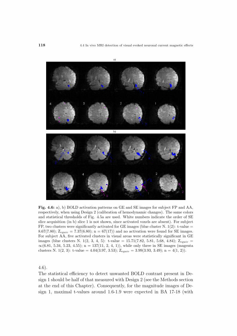
118 4.4 In vivo MRI detection of visual evoked neuronal current magnetic effects
Fig. 4.6: a), b) BOLD activation patterns on GE and SE images for subject FP and AA,respectively, when using Design 2 (calibration of hemodynamic changes). The same colorsand statistical thresholds of Fig. 4.5a are used. White numbers indicate the order of SEslice acquisition (in b) slice 1 is not shown, since activated voxels are absent). For subjectFP, two clusters were significantly activated for GE images (blue cluster N. 1(2): t-value =8.67(7.80); Zequiv = 7.37(6.80); n = 67(17)) and no activation were found for SE images.For subject AA, five activated clusters in visual areas were statistically significant in GEimages (blue clusters N. 1(2, 3, 4, 5): t-value = 15.71(7.82, 5.81, 5.68, 4.84); Zequiv =∞(6.81, 5.34, 5.23, 4.55); n = 137(11, 2, 4, 1)), while only three in SE images (magentaclusters N. 1(2, 3): t-value = 4.04(3.97, 3.53); Zequiv = 3.99(3.93, 3.49); n = 4(1, 2)).
4.6).
The statistical efficiency to detect unwanted BOLD contrast present in De-
sign 1 should be half of that measured with Design 2 (see the Methods section
at the end of this Chapter). Consequently, for the magnitude images of De-
sign 1, maximal t-values around 1.6-1.9 were expected in BA 17-18 (with

4. Neuronal current fMRI of in vivo visual evoked activity 119
even lower t-values in BA 19) for subject DD. This value is lower than the
t-threshold needed to achieve significance (t = 3.11, significance-level p <
0.001, uncorrected for multiple comparisons), and therefor no significant he-
modynamic changes were expected in the magnitude or phase SE images of
Design 1. In line with theoretical predictions, no signal changes related to
the BOLD contrast could be observed for this design (Design 1, threshold t
value equal to 3.11), in visual areas, nor for the 1st or the 2nd experimental
session for subject DD, see Fig 4.7.
On the contrary, phase changes (decreases) related to the modeled neuronal
currents were detected in one voxel pertaining to visual areas (Fig 4.7, cyan
arrow), close to the brain regions showing BOLD activations in GE images
(cluster 1). This was observed in both runs for the investigated subject, al-
though not exactly in the same location. Additional evidence, a necessary
but not a sufficient condition, that the observed phenomenon is really due to
neuronal currents and not of non-neuronal origin is the slice (4) in which it
occurred: indeed this slice corresponds to the one where the MRI acquisition
was synchronized with the presentation of the stimulus (together with slice
2, for an ascending slice acquisition order, see Fig. 4.2c). However concur-
rent activations (artefactual) in areas other than visual were present in the
same slices and no neuronal current induced phase changes in the opposite
direction (increases) were found in voxels adjacent to these significant phase
decreases.
With regard to magnitude images, no negatively activated voxels were found
in visual areas for any of the runs (ascending and descending slice acquisi-
tion order), neither in phase images (nor in the positive direction) for the
second run (descending slice acquisition order). For the other two subjects
no neuronal current activation were found, nor in magnitude, nor in phase
images.
4.5 Discussion and conclusions
In the present study, a first attempt to detect in vivo primary magnetic effects
of neuronal activity by spin-echo Magnetic Resonance images was conducted.
A fundamental prerequisite for a successful application of neuronal current
MRI is the discrimination between primary neuronal effects and secondary
hemodynamic-metabolic changes. For this purpose we chose to use a SE
instead of a GE technique because of its potential ability in this respect.
However, in order to achieve in vivo detection of such primary magnetic

120 4.5 Discussion and conclusions
Fig. 4.7: Neuronal and hemodynamic activation patterns for subject DD, when usingDesign 1 (detection of neuronal current effects). In a), and b), for the first and the sec-ond experimental session, respectively, superimposed on a BOLD GE magnitude imageare shown: in blue, positively activated voxels for BOLD GE magnitude images; inred/cyan positively/negatively activated voxels in SE phase images corresponding to neu-ronal event detection (fixed effects between two runs with ascending acquisition slice or-der); in magenta/green hemodynamic BOLD responses. White numbers indicate the orderof SE slice acquisition. One neuronal-current activated voxel (indicated by the cyan arrow)resulted in visual area BA 17, near BOLD GE (and also SE) activations, although notexactly in the same location at each measurement session (t-value equal to 3.35 and 3.58,and phase variations equal to -11 and -4 mrad for the 1st and the 2nd experimental session,respectively). It pertains to a slice (4) obtained in synchrony with the presentation of thestimulus (together with slice 2), see Fig. 4.2c. In slices without prior stimulus presentation(slices 1 and 3), no such significant signal variations could be observed. Drawn from [173].
field variations with SE techniques, the experimental approach had to be
optimized with respect to the contrast-to-noise and the recognizability of
the phenomenon. At this aim, we propose an approach that combines diffe-
rent measurement modalities: EEG based VEP recordings and conventional
BOLD fMRI with SE MR imaging of neuronal current-induced magnetic field
changes. In addition, by investigating the SE MRI time course in different
experimental designs we could further improve the precision of our approach.
The information related to the geometry (localization and orientation) of the
dipolar source, and its time-evolution could be determined by VEP recor-
dings. The knowledge of the dipolar source orientation was used to optimize
the effect of the expected magnetic field variations in SE MR images by pa-
tient and slice positioning orthogonal to the dipolar source. With regard to
orthogonalization of the dipolar orientation to the external field, this condi-

4. Neuronal current fMRI of in vivo visual evoked activity 121
tion could not always be achieved experimentally, due to geometric constrains
imposed by positioning inside the narrow bore of the MR scanner. In this
context, it was possible to achieve some optimization by selection of a visual
stimulus that facilitated subject positioning with regard to the geometry of
the dipolar source. In a general perspective, such adaptations may limit the
number of possible stimulation types that can be used in the experimental
situation. With regard to information driven by VEP recordings and by their
analysis, while it is well-known that the accuracy of the estimated dipolar
orientation and also the temporal resolution of VEP recordings are exquisite,
the spatial resolution may be of a more limited kind. Indeed, the localization
of the dipolar source, by which neuronal current MRI slice positioning was
guided, has an uncertainty of about 1 cm. For this reason, additional mea-
surement of BOLD activation patterns were used in order to improve spatial
localization of active regions, in terms of the accompanying hemodynamic re-
sponse. In this context, if possible, the acquisition of BOLD GE fMR images
could be done in a distinct MRI experimental session, prior to the neuronal-
current SE measurement: this information could then be used as constrains
for the spatial localization of the dipole estimated by the BESA algorithm.
Hereby, the definition of the active regions, needed for SE MRI slice position-
ing and for evaluation of neuronal current MRI activation patterns, would
be improved. Regarding the VEP component latencies, obtained for a given
subject and a specific stimulus, the TE of the SE sequence could be adapted
to match the VEP time evolution. In this respect, a precise synchronization
of the neuronal event with the MR SE acquisition had to be achieved by
carefully triggering the stimulus at defined time points with respect to the
MR sequence. Since the time-course of the dipolar source is on the order
of 100 ms, the time evolution of the first C1 peak could be accommodated
between the excitation and the refocusing pulse of the SE sequence. The re-
focusing of the expected magnetic field changes was thus avoided and thereby
the achievable contrast-to-noise ratio was increased. Besides, longer TEs also
affect the SNR; however, at 1.5 Tesla, the selected TE is on the order of the
transverse relaxation time in grey matter and a satisfying trade-off between
CNR and SNR could be obtained. The precise synchronization, within limits
given by physiological variation of the VEP signal time-course and stimulus
delivery, was also used to verify that really neuronal currents caused the ob-
served signal changes by an additional method: for each experimental run,
the stimulus was presented prior to acquisition of every second slice only,
that were shifted between runs to cover the active brain region. Indeed, sig-
nificant signal changes were observed in the stimulated slices alone, thereby
122 4.5 Discussion and conclusions
adding some confidence to our observations.
Beyond spatio-temporal synchronisation of stimulus presentation with MR
acquisition, there is another relevant issue: it regards the control of artefac-
tual contributions of non-neuronal origin to the signal, especially in terms of
stimulus induced hemodynamic changes, which constitute the BOLD signal
itself. In the present work neuronal and hemodynamic responses were mode-
led as two distinct contributions which add linearly to the signal (although
the neuronal signal also modulates the hemodynamic effect); in this context,
a stimulus timing (Design 1) was suggested and applied experimentally in
vivo that allowed concurrent estimation of both neuronal and hemodynamic
effects, rendering them de-correlated and hence estimable. The adoption of a
high frequency design (1 scan ON / 2 OFF cycle) gave a suitable solution to
the problem, although a complete de-correlation was not achieved. In a pre-
vious study, Xiong et al. [171] also adopted a high frequency design (1 scan
ON / 1 OFF), although the stimulus correlated signal was acquired at the
Nyquist frequency, that inevitably will lead to some loss of detection power.
Other solutions for de-correlating the neuronal and non-neuronal contribu-
tions can be found in the time domain. For example, by the use of designs
for which the distribution of the MN ⊗ iHRF term is normal, like latin-
square designs or geometric designs, as suggested for conventional BOLD
fMRI studies [162]. In addition, the use of m-sequences has been proposed
[191] to disentangle fast (neuronal and other effects) from slow (e.g. BOLD)
responses, neglecting the other component MN that we believe to contribute
independently to the signal. M-sequences were originally introduced in fMRI
studies to efficiently estimate the shape of the hemodynamic responses in
fast event-related experiments [192]; however, they suffer from low detection
efficiency for both first and second order responses, as noted by Kellman et
al. [193], in order to disentangle fast neuronal non-linearities from hemody-
namic effects.
With regard to the hardware configurations and acquisition strategies which
were optimized on phantoms, as discussed in the previous chapter, in the in
vivo study we applied the results regarding the coil type and the choice of the
bandwidth; on the contrary, the multi-echo sequence could not be used, since
the estimation model for the VEP signal dynamics was accommodated only
for the first component and was not optimized for later responses. However,
in future works with the development of more refined estimation methods,
multi-echo approaches may also help in the detection of neuronal current
primary effects.
Some results from the pilot study shown in the present work are encourag-

Application of neuronal current fMRI in vivo 123
ing. They indicate that magnetic effects caused by neuronal currents may
be detected in vivo by phase SE MR imaging: indeed these changes were
carefully synchronized with the acquisition, and could be registered close
to brain regions recorded as active by VEP and conventional BOLD fMRI.
Since these changes were observed in phase and not magnitude images, our
data seem to support the model of an extended oriented dipole, with mea-
surable effects within the dimension of the MRI voxel, as predicted by Konn
et al. [168]. This dipole corresponds to the source of scalp potential recor-
dings obtained by EEG(MEG), which is generally related to the extra(intra)-
cellular current of apical dendrites pertaining to pyramidal cells, oriented
radially(tangentially) to the scalp, as explained in Par. 1.2.3. The estimated
dipolar intensity of 27-50 nAm in the primary visual cortex for the subjects
investigated, in relation to previous calculations regarding extended dipoles
[168], actually may induce MR detectable phase changes. In the future, more
work has to be done to further validate detection of primary magnetic effects
caused by neuronal currents. In particular, results should be reproduced for
more subjects and different stimulation types; besides, more precise mod-
elling of the neuronal processes should be performed in order to account for
the different dipolar geometry of dendrites pertaining to both pyramidal and
non-pyramidal cells.
Materials and Methods
ParticipantsThree healthy subject (1 female, 2 males, age 27±2 yrs) volunteered to par-
ticipate in the study and gave their informed consent according to guidelines
reviewed and approved by local ethics authorities for work involving humans.
In the VEP experiment, the subjects were comfortably seated in a dimly lit
sound-attenuated and electrically shielded room, while in the MRI experi-
ment, the participants had to lay supine inside the magnet bore throughout
the experiment during the presentation of the visual stimuli. Positioning in
the MR system was performed so that the participant’s head would be ap-
proximately centred in the standing magnetic field and head movement was
minimized by mild restraint and cushioning together with the use of an indi-
vidually moulded bite bar.
ApparatusA Siemens Vision Magnetom MR system (Siemens Medical Systems, Erlan-
gen, Germany) operating at 1.5 Tesla and equipped for echo-planar imaging

124 Materials and methods
was employed for acquiring MR images. A flexible surface coil (size: 37 by
17 cm), was used for signal reception, while radio frequency transmission
was achieved by the body-coil. In the MRI experiment, visual stimuli were
projected via mirroring to a front projection screen using a LCD video pro-
jector (Model VPL-351QM, Sony Corp., Tokyo, refresh rate 60 Hz) located
inside the MR room and connected to a Dell Notebook CPx J750GT (600
MHz, 130.5 Mb RAM; Graphic card: ATI RAGE Mobility - M1 AGP2X,
8 Mb) located outside the MR room. Another PC, (Hewlett Packard Intel
Pentium, 48 Mb RAM, and software written in C++, Borland vers. 4.52,
running on MS-DOS) was used to record rectangular 5 V pulses from the
MR scanner and to send a counting trigger pulse to the Notebook serial port,
for synchronization of the stimulus presentation with MRI acquisition. At
specific delays after trigger delivery, the notebook started the stimulus pre-
sentation (guided by in-house software written in Cogent 2000, vers. 1.25).
The achieved synchronization precision between MR-scanning and stimulus
presentation was within a few ms. MR image analyses were performed with
software (see “MRI analysis”) running on LINUX (Debian 3.0), on an IBM
server (xSeries 235, Intel Xeon 2.4 GHz dual processor). In the VEP experi-
ment, the EEG was recorded from 64 electrodes placed according to the 10-10
system montage; for details see [190]. Visual stimuli were presented for each
of the visual quadrants on a video monitor with a refresh rate of 60 Hz, at
a viewing distance of 57 cm, controlled by the DOS based STIMTM stimula-
tion software (Neuroscan inc, USA) running on an PC (Intel Pentium III,
650 MHz, 256 Mb RAM, Graphic card: ETI 6000 Direct Draw - 3.50 Mb)
which also tagged the EEG acquisition. EEG recordings and VEP analysis
was performed on a PC (Intel Pentium IV, 1.80 GHz, 512 Mb RAM) using
the Brain Vision system (Brain Products GmbH, Germany) that includes the
software Vision Recorder and Vision Analyzer.
StimuliThe stimulus (Fig. 4.2b), consisted in a checkerboard segment (windmill)
starting 3 from the fixation point and extending laterally for 14 of the visual
angle (basis 9). A central cross (0.2) was employed as fixation point. The
spatial frequency was 2 cycles/degree. The background luminance (22 cd/m2)
was isoluminant with the mean luminance of the grating pattern, which was
modulated at a contrast of 32%. The centre of the stimulus was displayed at
polar angle of 25 above the horizontal meridian. This stimulus was binoc-
ularly presented for 50 ms in the upper left quadrant of the visual field (in
the VEP experiment also in the other quadrants, for control), alternated to
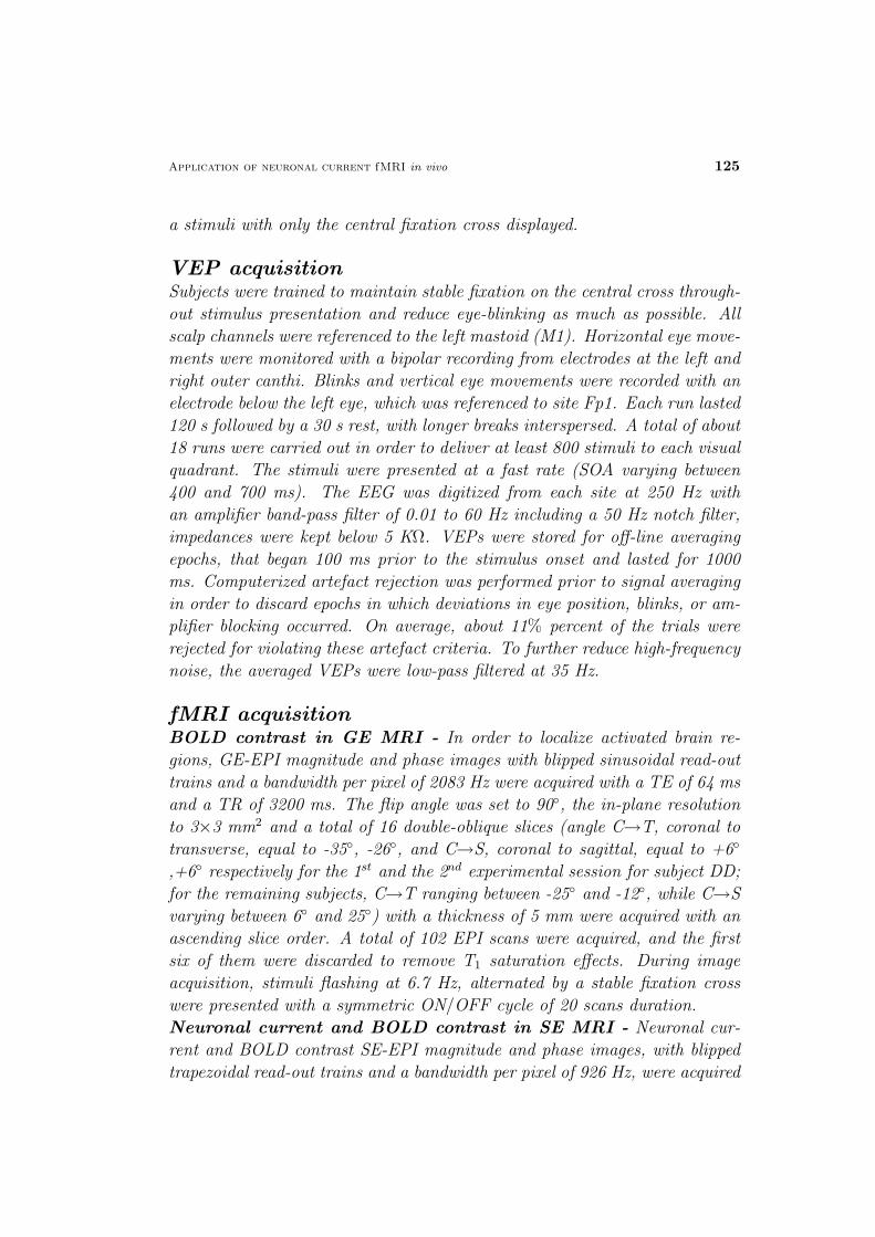
Application of neuronal current fMRI in vivo 125
a stimuli with only the central fixation cross displayed.
VEP acquisitionSubjects were trained to maintain stable fixation on the central cross through-
out stimulus presentation and reduce eye-blinking as much as possible. All
scalp channels were referenced to the left mastoid (M1). Horizontal eye move-
ments were monitored with a bipolar recording from electrodes at the left and
right outer canthi. Blinks and vertical eye movements were recorded with an
electrode below the left eye, which was referenced to site Fp1. Each run lasted
120 s followed by a 30 s rest, with longer breaks interspersed. A total of about
18 runs were carried out in order to deliver at least 800 stimuli to each visual
quadrant. The stimuli were presented at a fast rate (SOA varying between
400 and 700 ms). The EEG was digitized from each site at 250 Hz with
an amplifier band-pass filter of 0.01 to 60 Hz including a 50 Hz notch filter,
impedances were kept below 5 KΩ. VEPs were stored for off-line averaging
epochs, that began 100 ms prior to the stimulus onset and lasted for 1000
ms. Computerized artefact rejection was performed prior to signal averaging
in order to discard epochs in which deviations in eye position, blinks, or am-
plifier blocking occurred. On average, about 11% percent of the trials were
rejected for violating these artefact criteria. To further reduce high-frequency
noise, the averaged VEPs were low-pass filtered at 35 Hz.
fMRI acquisitionBOLD contrast in GE MRI - In order to localize activated brain re-
gions, GE-EPI magnitude and phase images with blipped sinusoidal read-out
trains and a bandwidth per pixel of 2083 Hz were acquired with a TE of 64 ms
and a TR of 3200 ms. The flip angle was set to 90, the in-plane resolution
to 3×3 mm2 and a total of 16 double-oblique slices (angle C→T, coronal to
transverse, equal to -35, -26, and C→S, coronal to sagittal, equal to +6
,+6 respectively for the 1st and the 2nd experimental session for subject DD;
for the remaining subjects, C→T ranging between -25 and -12, while C→S
varying between 6 and 25) with a thickness of 5 mm were acquired with an
ascending slice order. A total of 102 EPI scans were acquired, and the first
six of them were discarded to remove T1 saturation effects. During image
acquisition, stimuli flashing at 6.7 Hz, alternated by a stable fixation cross
were presented with a symmetric ON/OFF cycle of 20 scans duration.
Neuronal current and BOLD contrast in SE MRI - Neuronal cur-
rent and BOLD contrast SE-EPI magnitude and phase images, with blipped
trapezoidal read-out trains and a bandwidth per pixel of 926 Hz, were acquired

126 Materials and methods
in separate runs after optimization of the TE to reflect VEP dynamics. The
flip angle was set to 70 and a total of 390 images with a TE of 100 ms,
and TR of 1.3 s were acquired. The first six images were discarded from
further analysis to remove any possible T1 saturation effects. The in-plane
resolution and positioning of slices were the same as for the BOLD GE-MRI
session, but only 4 slices were acquired in a descending or ascending order.
During image acquisition, the stimulus presentation was varied according to
two experimental designs.
Design 1 (neuronal current detection): stimuli flashing at 1.7 Hz, alternated
by a stable fixation cross were presented with a 1 scan ON/ 2 scans OFF
cycle. During the ON-period, 2 stimuli were presented each synchronized to
2 out of the 4 slices. A total of two runs was acquired, both for the ascending
and the descending slice orders (Fig. 4.2c).
Design 2 (BOLD SE-MRI calibration) - stimuli flashing at 1.7 Hz, alternated
by a stable fixation cross were presented with a 20 scans ON/OFF cycle. Only
one run (ascending acquisition order) was performed. Since the efficiency ra-
tio E1/E2 for estimating hemodynamic effects of Design 1 and Design 2 is
about 0.5, expected statistical t-values related to hemodynamic changes for
Design 1 will be half of those detected for Design 2.
The presentation of the stimuli was synchronized with MR acquisition: as
outlined in Fig 4.2a, appropriate delays between stimulus onset and the ex-
citation pulse was chosen according to the dipolar source onset latency (see
below) with respect to the stimulus onset. Patient positioning was performed
in order to othogonalise as far as possible the dipolar orientation, estimated by
the VEP recordings to the external field B0. Likewise, slice positioning (kept
invariant during each MRI session) was performed on the basis of dipolar
localization (in terms of Tailarach coordinates) obtained by the VEP analy-
sis (see below), and were oriented orthogonal to the dipolar orientation (Fig.
4.3a,b), resulting in a double oblique slice, see Fig. 4.3bc,d. Only subject DD
participated in two experimental MRI sessions, performed on different days;
the remaining came only once.
ERP analysisEstimation of the dipolar sources of VEP components was carried out us-
ing Brain Electrical Source Analysis (BESA 2000 version 5.1, MEGIS Soft-
ware GmbH, Germany). The BESA algorithm estimates the location and
the orientation of multiple equivalent dipolar sources by calculating the scalp
distribution that would be obtained for a given dipolar model (forward solu-
tion) and comparing it to the actual VEP distribution. Interactive changes
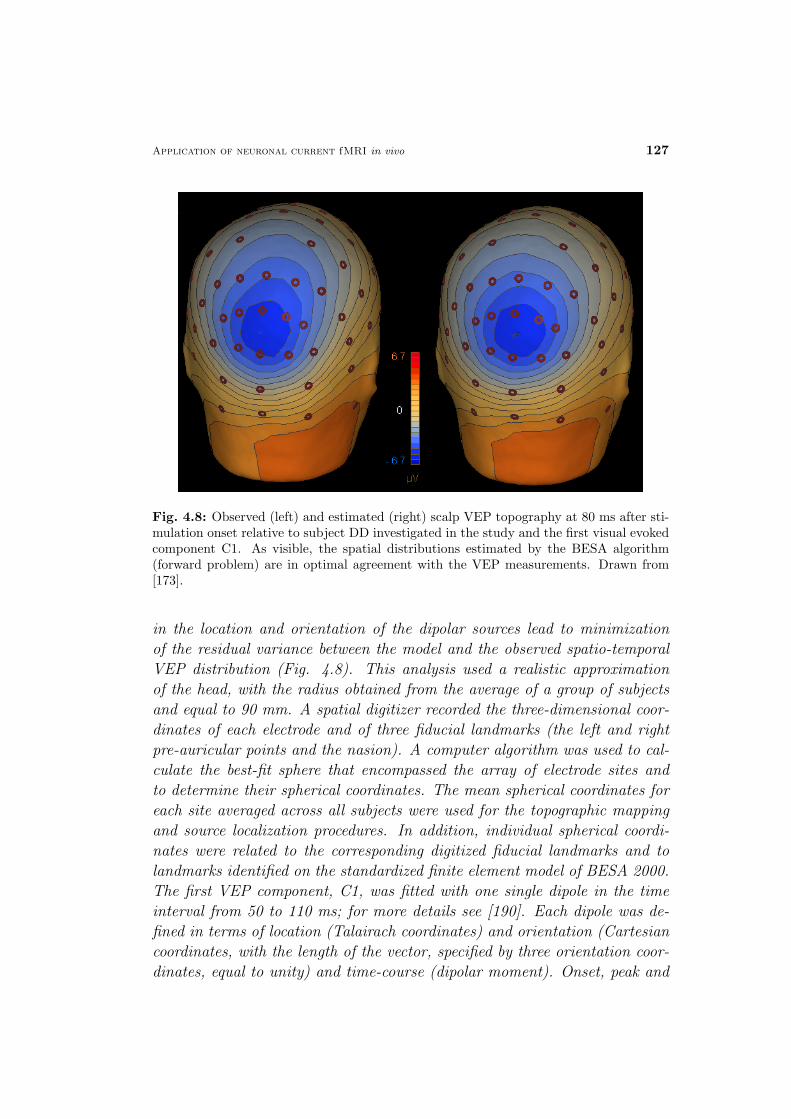
Application of neuronal current fMRI in vivo 127
Fig. 4.8: Observed (left) and estimated (right) scalp VEP topography at 80 ms after sti-mulation onset relative to subject DD investigated in the study and the first visual evokedcomponent C1. As visible, the spatial distributions estimated by the BESA algorithm(forward problem) are in optimal agreement with the VEP measurements. Drawn from[173].
in the location and orientation of the dipolar sources lead to minimization
of the residual variance between the model and the observed spatio-temporal
VEP distribution (Fig. 4.8). This analysis used a realistic approximation
of the head, with the radius obtained from the average of a group of subjects
and equal to 90 mm. A spatial digitizer recorded the three-dimensional coor-
dinates of each electrode and of three fiducial landmarks (the left and right
pre-auricular points and the nasion). A computer algorithm was used to cal-
culate the best-fit sphere that encompassed the array of electrode sites and
to determine their spherical coordinates. The mean spherical coordinates for
each site averaged across all subjects were used for the topographic mapping
and source localization procedures. In addition, individual spherical coordi-
nates were related to the corresponding digitized fiducial landmarks and to
landmarks identified on the standardized finite element model of BESA 2000.
The first VEP component, C1, was fitted with one single dipole in the time
interval from 50 to 110 ms; for more details see [190]. Each dipole was de-
fined in terms of location (Talairach coordinates) and orientation (Cartesian
coordinates, with the length of the vector, specified by three orientation coor-
dinates, equal to unity) and time-course (dipolar moment). Onset, peak and

128 Materials and methods
offset latencies were then established for the components of interest, C1, by
averaging EEG traces in phase with stimulus delivery.
MRI analysisMovement artefacts were assumed negligible, since motion correction parame-
ters did not exceed 1 mm for translations and 0.5 for rotations. Phase image
pre-processing was performed with software developed in Matlab, version 6.0
(The MathWorks, Inc., Natick, MA; USA): each phase time-series was un-
wrapped over time and then linearly detrended. Both magnitude and phase
images were then analyzed by SPM2 (Statistical Parametric Mapping, Well-
come Department of Imaging Neuroscience, London, UK,
http://www.fil.ion.ucl.ac.uk/spm/spm2.html). BOLD GE-EPI magnitude ima-
ges were spatially smoothed (FWHM = 6 mm) and temporally regularized for
colored noise: high-pass temporal filtering, with cut-off frequency νC equal to
1/128 Hz, was applied, followed by autocorrelation estimation of the resid-
uals, assuming a first-order autoregressive model plus white noise. Linear
regression with only the modelled hemodynamic response, MH , was calcu-
lated, since no synchronization with the neuronal event was carried out. In
particular, MH was obtained, as in Eq. 4.4, with the kernel iHRF equal to
the SPM2 canonical hemodynamic response function. Activation maps are
displayed for a statistical threshold p = 0.05, corrected for family-wise error
and with a minimum number of voxels in a cluster equal to 2. Activated areas
were normalized to a standard brain by SPM2. Both phase and magnitude
SE-EPI images were temporally high-pass filtered (νC = 1/128 Hz). No spa-
tial smoothing was applied, because, in phase images, adjacent positive and
negative variations could sum to zero for a symmetric configuration of the
voxels with respect to the neuronal source and negative interference would oc-
cur in case of smoothing. The design matrix employed in the linear regression
comprised, in this case, both a modelled hemodynamic response, MH , and a
neuronal response MN (see Eq. 4.3) and effect sizes h and n were estimated.
The shape of the kernel iHRF of Eq. 4.4 and 4.5 was assumed equal to the
SPM2 canonical hemodynamic response function (see Fig. 1.15b) for both
magnitude and phase images; besides MN , consisting of ones when the event
occurred and zeros elsewhere (FIR model of order 1 and a window length
equal to the TR, see Fig 4.4). Activation maps are displayed for a statistical
threshold p = 0.001, uncorrected for multiple comparisons. Temporal signal
to noise ratio (SNR) was computed voxel-wise on magnitude SE images after
linear detrending (mean signal divided by its standard deviation over time).
Chapter 5
Conclusions and perspectives
In this PhD thesis, we discussed the feasibility of detecting by MRI magnetic
effects induced by neuronal currents in vivo, a cutting edge fMRI technique.
With regard to MRI sensitivity, in literature findings showed that, for cur-
rents induced in phantoms, magnetic field distortion of a few tenths of nTesla
can be detected at 3 Tesla [167, 168]. In the present thesis, we extended this
result to a magnetic field strength of 1.5 Tesla [173], showing that optimized
acquisitions, the use of multi-spin-echo approaches and improved hardware
performances at low fields lead to results close to that obtained at twice
the field strength. The minimum detected magnetic field changes are com-
parable in amplitude to that of neuronal currents in the human brain, as
estimated from MEG measurements [166–168] or by direct modeling [168].
However, these changes are at the detection limit of MRI and neuronal cur-
rent effects may be confounded by false positives due to the noise. At this
regard, increases in sensitivity are needed and, auspiciously, future technical
improvement may push this limit even further. Besides, more modeling ef-
forts would help to forecast neuronal current induced MR signal changes and
to interpret better in vivo results.
With previous studies and with the present work, advances have been made,
with regard to the setting of the acquisition parameters for a neuronal cur-
rent fMRI experiment. Several works [166–168], as described in Par. 3.1,
have demonstrated how the choice of acquisition technique and type of MR
image (magnitude or phase images) can positively affect the detection limit
of weak magnetic field changes relative to induced currents in phantoms.
Phase images are more sensitive to weak magnetic field changes than magni-
tude images, as shown for extended dipoles [168]; spin-echo techniques should
enable the discrimination of fast neuronal processes from other with slower
129
130 Conclusions and perspectives
time-scales. However, on one hand the combined use of spin-echo techniques
and phase images enabled the detection of spontaneous neuronal activity (at
a spiking rate of about 0.15 Hz), as demonstrated in neuronal cell-cultures
[170]. On the other hand, the only successful and consistent experimental
evidence [171] over six subjects of a direct detection of neuronal current mag-
netic effects in vivo were obtained by the use of magnitude GE images.
We decided to acquire SE images, synchronized with the visual evoked re-
sponse: in this way we could constrain the BOLD signal and positively add
the effect of evoked components of opposite sign. We also constrained and
calibrated possible unwanted BOLD signal contributions by the use of two
different appropriate stimulation designs. For the first time, by the use of
SE phase images, magnetic effects due to neuronal evoked responses were
detected [173]. Our result is encouraging, however it has to be confirmed
more systematically on more subjects and for more stimulus types.
We are planning to investigate the feasibility of measuring primary effects
of neuronal current for situations when the amplitude of electric activity is
greater than that of evoked responses in healthy subjects. This is the case
for paroxysmal responses in visual areas of epileptic patients, with fixation
off sensitivity (FOS) epilepsy [197, 198]. The advantage of this type of elec-
trical activity (2-3 Hz waves) elicited by the loss of fixation, for example eyes
closing, is first of all in their intensity, which is at least twice with respect
to spontaneous alpha waves (see Fig. 4.1); besides in their lower frequency,
which, in terms of MR acquisition, implies the adoption of longer TRs, with
significant gains in SNR (see Fig. 4.1); finally, as opposite to alpha waves,
the advantage of a precise brain location where this epileptic activity takes
place, e.g. the lateral occipital lobe. At this aim, we plan the investigation
of both the hemodynamic and the electric responses by MRI and EEG re-
cordings, to the elimination of fixation, but also during visual stimulation.
In conclusion, on the basis of theoretical and experimental investigation, the
feasibility of detecting neuronal currents by fMRI is at the limits of current
MR technology. Nevertheless by MRI, unexpectedly ultra-weak magnetic
field changes can be detected. Besides, several modeling and experimental
improvements were achieved, which may be helpful for future works.
Possible advantages and limitations of neuronal current fMRI have been elu-
cidated. Neuronal current fMRI maps may furnish information regarding
the location of the activity with the best precision with respect to all the
other currently employed techniques for the non-invasive study of human
brain function. Its spatial, as well its temporal resolution is determined by
the MRI technique alone, as opposed to the BOLD fMRI approach which

Conclusions and perspectives 131
is limited by the features of the physiological response. However, neuronal
current fMRI alone may not be practical, since several information regarding
the electric source timing, location and orientation are of importance, that
must be furnished by other techniques (EEG/MEG).
We conclude that more experimental evidences are needed in order to estab-
lish the feasibility of detecting magnetic effects induced by neuronal currents
in vivo, auspicably with improved MR technology.

References
[1] Broca P, Brown-Sequard CE. Proprietes et fonctions de la moelle epiniere:rapport quelques experiences de M. Borwn-Sequard. Lu a la Societe de biologies le21 Juillet (Bonaventure et Ducessois) 1: 201 (1855).
[2] Roland PE. Brain activation. New York: John Wiley and Sons (1993).
[3] Kandel ER. Principles of neural science. Amsterdam: Elsevier Science publication(1991).
[4] Logothetis N. The underpinnings of the BOLD functional magnetic resonanceimaging signal. J Neurosci 23: 3963–3971 (2003).
[5] Logothetis N. The neural basis of the blood-oxygen-level-dependent functionalmagnetic resonance imaging signal. Phil Trans R Soc Lond B 357: 1003–1037(2002).
[6] Logothetis N, Pauls J, Augath M, Trinath T, Oeltermann A. Neuro-physiological investigation of the basis of the fMRI signal. Nature 412: 150–157(2001).
[7] Almeida R, Stetter M. Modeling the link between functional imaging and neu-ronal activity: synaptic metabolic demand and spike rates. Neuroimage 17: 1065–1079 (2002).
[8] Bandettini PA, Ungerleider LG. From neuron to BOLD: new connections.Nat Neurosci 4: 864–866 (2001).
[9] Orrison WW, Lewine JD, Sanders JA, Hartshorne MF. Functional brainimaging. Mosby Ed., St. Louis (1995).
[10] Gevins A. Electrophysiological imaging of brain function. In: Toga Aw, MazziottaJC, editors. Brain Mapping: the methods. San Diego: Academic Press; pp 259–276(1996).
[11] Romani GL. Fundamentals on neuromagnetism. In: Williamson SJ, Hoke M,Stroink G, Kotani M, editors. Advances in Biomagnetism. New York: Plenum Press;pp 87–92 (1990).
[12] Darvas F, Pantazis D, Kucukaltun-Yildirim E, Leahy RM. Mapping humanbrain fucntion with MEG and EEG: methods and validation. Neuroimage 23: S289–S299 (2004).
[13] Polich J. Detection change: event-related potential and fMRI findings. Dordrecht:Kluwer Academic Publishers (2003).
133
134 References
[14] Peppiatt C, Attwell D. Feeding the brain. Nature 431: 137–138 (2004).
[15] Mosso A. Uber den Kreislauf des Blutes im Menschlichen Gehirn (von Veit,Leipzig, 1881).
[16] Roy CS, Sherrington CS. On the regulation of blood supply of the brain. JPhisiol 11: 85–108 (1890).
[17] Attwell D, Iadecola C. The neural basis of functional brain imaging signals.Trends Neurosci 25: 621–625 (2002).
[18] Attwell D, Laughlin SB. An energy budget for signaling in the grey matter ofthe brain. J Cereb Blood Flow Metab 21: 1133–1145 (2001).
[19] Kuschinsky W. Regulation of cerebral blood flow. In: Moonen CTW, BandettiniPA, editors. Functional MRI. Berlin: Springer; pp 15–24 (1999).
[20] Malonek D, Grinvald A. Interactions between electrical activity and corticalmicrocirculation revealed by imaging spectroscopy: implications for functional brainmapping. Science 272: 551–554 (1996).
[21] Kim DS, Duong DQ, Kim SG. High resolution mapping of iso-orientation columnsby fMRI. Nat Neurosci 3: 164–169 (2000).
[22] Buxton RB, Uludag K, Dubowitz DJ, Liu TT. Modeling the hemodynamicresponse to brain activation. Neuroimage 23: S220–S233 (2004).
[23] Grubb RL, Raichle ME, Eichling JO, Ter-Pogossian MM. The effects ofchanges in PaCO2 on cerebral blood volume, blood flow and vascular mean transittime. Stroke 5: 630–639 (1974).
[24] Buxton Rb, Wong Ec, Frank LR. Dynamics of blood flow and oxygenationchanges during brain activation: the balloon model. Magn Reson Med 39: 855–864(1998).
[25] Mandeville JB, Marota JJA, Ayata C, Zaharchuk G, Moskowitz MA,
Rosen BR, Weisskoff RM. Evidence of a cerebro-vascular post-arteriole Wind-kessel with delayed compliance. J Cereb Blood Flow Metab 19: 679–689 (1999).
[26] Aubert A, Costalat R. A model of the coupling between brain electrical activ-ity, metabolism and hemodynamics: application to the interpretation of functionalneuroimaging. Neuroimage 17: 1162–1181 (2002).
[27] Clarke DD, Sokoloff L. Circulation and energy metabolism of the brain. In:Siegel GJ, Agranoff BW, Wayne Albers R, Molinoff PB, editors. Basic neurochem-istry: molecular, cellular and medical aspects. New York: Raven Press; pp 645–680(1994).
[28] Gjeddie A. The relation between brain function and cerebral blood flowand metabolism. In: Batjer HH, editor. Cerebrovascular desease. Philadelphia:Lippincott-Raven; pp 23–40 (1997).
[29] Creutzfeld OD. Neurophysiological correlates of different functional states ofthe brain. In: Ingvar DH, Lassen NA, editors. Alfred Benzon Symposium VIII. NewYork: Academic Press; pp 21–46 (1975).
[30] Villringer A. Physiological changes during brain activation. In: Moonen CTW,Bandettini PA, editors. Functional MRI. Berlin: Springer; pp 3–13 (1999).
References 135
[31] Nudo Rj, Masterton RB. Stimulation-induced [14 C]2-deoxyglucose labeling ofsynaptic activity in the cerebral auditory system. J Comp Neurol 245: 553–565(1986).
[32] Lauritzen M. Relationship of spikes, synaptic activity and local changes of cerebralblood flow. J Cereb Blood Flow Metab 21: 1367–1383 (2001).
[33] Walvodgel D, van Gelderen P, Muellbacher W, Ziemann U, Immisch I,
Hallett M. The relative metabolic demand of inhibition and excitation. Nature406: 995–998 (2000).
[34] Sokoloff L. Circulation and energy metabolism of the brain. In: Siegel GJ, Agra-noff BW, Wayne Albers R, Molinoff PB, editors. Basic neurochemistry: molecular,cellular and medical aspects. New York: Raven Press; pp 565–590 (1989).
[35] Edvinson L, MacKenzie ET, McCulloch J. Cerebral blood flow andmetabolism. (Raven, New York): 161 (1993).
[36] Sokoloff L. Localization of functional activity in the central nervus system bythe measurement of glucose utilization with radioactive deoxyglucose. J Cereb BloodFlow Metab 1: 7–36 (1981).
[37] Hatazawa J, Ito M, Matsuzawa T, Ido T, Watanuki S. Measurement of theratio of cerebral oxygen consumption to glucose utilization by positron emission to-mography: its consistency with the values determined by the Kety-Schmidt methodin normal volunteers. J Cereb Blood Flow Metab 8: 426–432 (1988).
[38] Fox PT, Raichle ME. Focal physiological uncoupling of cerebral blood flow andoxidative metabolism during somatosensory stimulation in human subjects. ProcNat Acad Sci USA 83: 1140–1144 (1986).
[39] Fox PT, Raichle ME, Mintun MA, Dence C. Nonoxydative glucose consum-ption during focal physiologic neural activity. Science 241: 462–464 (1988).
[40] Ribeiro L et al . Cerebral blood flow and metabolysm during nonspecific bilateralvisual stimulation in normal subjects. In: Uemura K et al., editors. Quantificationof brain function. Tracer kinetics and image analysis in brain PET. Amsterdam:Elsevier Science Publication; pp 229–234 (1993).
[41] Blomqvist G, Seitz RJ, Sjogren I, Halldin C, Stone-Elander S, Widen
L, Solin O, Haaparanta M. Regional cerebral oxidative and total glucose con-sumption during rest and activation studied with positron emission tomography.Acta Physiol Scand 151: 29–43 (1994).
[42] Madsen PL, Hasselbalch SG, Hagemann LP, Olsen KS, Bulow J, Holm
S, Wildschiodtz G, Paulson OB, Lassen NA. Persistent resetting of thecerebral oxygen/glucose uptake ratio by brain activation: evidence obtained withthe Kety-Schmidt technique. J Cereb Blood Flow Metab 15: 485–491 (1995).
[43] Chen W, Novotny EJ, Zhu XH, Rothman DL, Shulman RG. Localized 1HNMR measurement of glucose consumption in the human brain visual stimulation.Proc Nat Acad Sci USA 90: 9896–9900 (1993).
[44] Frahm J, Krueger G, Merboldt KD, Kleinschmidt A. Dynamic uncouplingand recoupling of perfusion and oxidative metabolism during focal brain activationin man. Magn Reson Med 35: 143–148 (1996).
136 References
[45] Frahm J, Krueger G, Merboldt KD, Kleinschmidt A. Dynamic NMRstudies of perfusion and oxidative metabolism during focal brain activation. AdvExp Med Biol 413: 195–203 (1997).
[46] Giove F, Mangia S, BianciardiM , Garreffa G, Di Salle F, Morrone R,
Maraviglia B. The physiology and metabolism of neuronal activation: in vivostudies by NMR and other methods. Magn Reson Imag 21: 1283–1293 (2003).
[47] Prichard J, Rothman D, Novotny E, Petroff O, Kuwabara T, Avison
M, Howseman A, Hanstock C, Shulman R. Lactate rise detected by 1H- NMRin human visual cortex during physiologic stimulation. Proc Nat Acad Sci USA 88:5829–5831 (1991).
[48] Sappey-Marinier D, Calabrese G, Fein G, Hugg JW, Biggins C, Weiner
MW. Effect of photic stimulation on human visual cortex lactate and phosphatesusing 1H and 31P magnetic resonance spectroscopy. J Cereb Blood Flow Metab 12:584–592 (1992).
[49] Jenkins BG, Belliveau JW, Rosen BR. Confirmation of lactate productionduring photic stimulation. Improved protocols using inter- and intra-subject aver-aging. In: Proc Soc Magn Reson Med (SMRM), 11th annual scientific meeting 2:2145 (1992).
[50] Merboldt KD, Bruhn H, Hanicke W, Michaelis T, Frahm J. Decrease ofglucose in the human visual cortex during photic stimulation. Magn Reson Med 25:187–194 (1992).
[51] Pellerin L, Magistretti PJ. Glutamate uptake into astrocytes stimulates ae-robic glycolysis: a mechanism coupling neuronal activity to glucose utilization. ProcNat Acad Sci USA 91: 10625–10629 (1994).
[52] Magistretti PJ, Hof PR, Martin JL. Adenosine stimulates glycogenolysis inmouse cerebral cortex: a possible coupling mechanism between neuronal activityand energy metabolism. J Neurosci 6: 2558–2562 (1986).
[53] Pellerin L, Pellegri G, Bittar PG, Charnay Y, Bouras C, Martin JL,
Stella N, Magistretti PJ. Evidence supporting the existence of an activity-dependent astrocyte-neuron lactate shuttle. Dev Neurosci 20: 291–299 (1998).
[54] Pierre K, Pellerin L, Debernardi R, Riederer BM, Magistretti PJ.Cell-specific localization of monocarboxylate transporters, MCT1 and MCT2, in theadult mouse brain revealed by double immunohistochemical labeling and confocalmicroscopy. Neuroscience 100: 617–627 (2000).
[55] Magistretti PJ. Cellular basis of functional brain Imaging: insights from neuron-glia metabolic coupling. Brain Res 886: 108–112 (2000).
[56] Vannucci SJ, Maher F, Simpson IA. Glucose transporter proteins in brain:delivery of glucose to neurons and glia. Glia 21: 2–21 (1997).
[57] Takahashi S, Driscoll BF, Law MJ, Sokoloff L. Role of sodium and potas-sium ions in regulation of glucose metabolism in cultured astroglia. Proc Nat AcadSci USA 92: 4616–4620 (1995).
References 137
[58] Gjeddie A, Marrett S. Glycolysis in neurons, not astrocytes, delays oxidativemetabolism of human visual cortex during sustained checkerboard stimulation invivo. J Cereb Blood flow Metab 21: 1384–1392 (2001).
[59] Chih CP, He J, Sly TS, Roberts EL Jr. Comparison of glucose and lactate assubstrate during NMDA- induced activation of hippocampal slices. Brain Res 893:143–154 (2001).
[60] Mangia S, Garreffa G, BianciardiM , Giove F, Di Salle F, Maraviglia
B. The aerobic brain: lactate decrease at the onset of neural activity. Neuroscience118: 7–10 (2003).
[61] Kasischke KA, Vishwasrao HD, Fisher PJ, Zipfel WR, Webb WW. Neuralactivity triggers neuronal oxidative metabolism followed by astrocytic glycolysis.Science 305: 99–103 (2004).
[62] Chih CP, Lipton P, Roberts EL Jr. Do active cerebral neurons really uselactate rather than glucose?. Trends Neurosci 24: 573–578 (2001).
[63] Mangia S, Giove F, BianciardiM , Di Salle F, Garreffa G, Maraviglia
B. Issues concerning the construction of a metabolic model for neuronal activation.J Neurosci Res 71: 463–467 (2003).
[64] Seitz RJ, Roland PE. Vibratory stimulation increases and decreases the regionalcerebral blood flow and oxydative metabolism: a positron emission tomography(PET) study. Acta Neurol. Scand. 86: 60–67 (1992).
[65] Marrett S, Gjeddie A. Changes of blood flow and oxygen consumption in visualcortex of living humans. In: Villringer A et al., editors.Optical Imaging of BrainFunction and Metabolism II New York: Plenum Press; pp 205–208 (1997).
[66] Roland PE, Eriksson L, Stone-Elander S, Widen L. Does mental activitychange the oxydative metabolism of the brain? J Neurosci 7: 2373–2389 (1987).
[67] Marrett S et al . Stimulus specific increase of oxidative metabolism in humanvisual cortex. In: Uemura K et al., editors. Quantification of brain function. Tracerkinetics and image analysis in brain PET Amsterdam: Elsevier Science Publication;pp 217–224 (1993).
[68] Davis TL, Kwong KK, Weisskoff RM, Rosen BR. Calibrated functionalMRI: mapping the dynamics of oxidative metabolism. Proc Nat Acad Sci USA 95:1834–1839 (1998).
[69] Villringer A, Chance B. Non-invasive optical spectroscopy and imaging ofhuman brain function. Trends Neurosci 20: 435–442 (1997).
[70] Malonek D, Grinvald A. Vascular regulation at submillimiter range. Adv ExpMed Biol 413: 215–220 (1997).
[71] Villringer A, Planck J, Hock C, Schleinkofer L, Dirnagl U. Near infraredspectroscopy (NIRS): a new tool to study hemodynamic changes during activationof brain function in human adults. Neurosci. Lett. 154: 101–104 (1993).
[72] Meek JH, Elwell CE, Khan MJ, Romaya J, Wyatt JS, Delpy DT, Zeki S.Regional changes in cerebral hemodynamics as a result of a visual stimulus measuredby near infrared spectroscopy. Proc R Soc Lond B: Biol Sci 261: 351–356 (1995).

138 References
[73] Wenzel R, Obrig H, Ruben J,Villringer K, Thiel A, Bernarding J,
Dirnagl U, Villringer A. Cerebral blood oxygenation changes induced by visualstimulation in humans. J Biomed Opt 1: 399–404 (1996).
[74] Obrig H, Hirth C, Junge-Hulsing JG, Doge C, Wolf T, Dirnagl U, Vill-
ringer A. Cerebral oxygenation changes in response to motor stimulation. J. Appl.Physiol. 81: 1174–1183 (1996).
[75] Frostig RD, Lieke EE, Ts’O DY, Grinvald A. Cortical functional architectureand local coupling between neuronal activity and the microcirculation revealed byin vivo high-resolution optical imaging of intrinsic signals. Proc Nat Acad Sci USA87: 6082–6086 (1990).
[76] Buxton RB. The elusive initial dip. Neuroimage 13: 953–958 (2001).
[77] Lindauer U, Royl G, Leithner C, Kuhl M, Gold L, Gethmann J, Kohl-
Bareis M, Villringer A, Dirnagl U. No evidence for early decrease in bloodoxygenation in rat whisker cortex in response to functional activation. Neuroimage13: 988–1001 (2001).
[78] Jones M, Berwick J, Johnston D, Mayhew J. Concurrent optical imagingspectroscopy and laser-Doppler flowmetry: the relationship between blood flow,oxygenation, and volume in rodent barrel cortex. Neuroimage 13: 1002–1015 (2001).
[79] Ernst T, Hennig J. Observation of a fast response in furnctional MR. MagnReson Med 32: 146–149 (1994).
[80] Menon RS, Ogawa S, Strupp JP, Anderson P, Ugurbil K. BOLD basedfunctional MRI at 4T includes a capillary bed contribution: echo-planar imagingcorrelates with previous optical imaging using intrinsic signal. Magn Reson Med 33:453–459 (1995).
[81] Hu X, Le TH, Ugurbil K. Evaluation of the early response in fMRI in individualsubjects using short stimulus duration. Magn Reson Med 37: 877–884 (1997).
[82] Yacoub E, Hu X. Detection of the early decrease in fMRI signal in the motorarea. Magn Reson Med 45: 184–190 (2001).
[83] Yacoub E, Hu X. Detection of the early negative response in fMRI at 1.5T. MagnReson Med 41: 1088–1092 (1999).
[84] Fransson P, Kruger G, Merboldt K, Frahm J. Temporal characteristics ofoxygenation-sensitive MRI response to visual activations in humans. Magn ResonMed 39: 912–919 (1998).
[85] Silva AC, Lee SP, Iadecola C, Kim SG. Early temporal characteristics of cere-bral blood flow and deoxyhemoglobin changes during somatosensory stimulation. JCereb Blood Flow Metab 20: 201–206 (2000).
[86] Bandettini PA, Wong EC, Binder R, Rao SM, Jesmanowicz A, Aaron
EA, Lowry T, Forster HV, Hinks RS, Hyde JS. Functional MR imagingusing the BOLD approach: dynamic characteristics and data anlysis methods. In:Le Bihan D, editor. Diffusion and perfusion Magnetic Resonance New York: RavenPress; pp 335–349 (1995).
References 139
[87] Kruger G, Kleinschmidt A, Frahm J. Dynamic MRI sensitized to cerebralblood oxygenation and flow during sustained activation of human visual cortex.Magn Reson Med 35: 797–800 (1996).
[88] Lu H, Golay X, Pekar JJ, Van Zijl PC . Functional magnetic resonanceimaging based on changes in vascular space occupancy. Magn Reson Med 50: 263–274 (2003).
[89] Li TQ, Haefelin TN, Chan B, Kastrup A, Jonsson T, Glover GH, Mose-
ley ME. Assessment of hemodynamic response during focal neural activity in hu-man using bolus tracking, arterial spin labeling and BOLD techniques. Neuroimage12: 442–451 (2000).
[90] Hoge RD, Atkinson J, Gill B, Crelier GR, Marrett S, Pike GB. Linearcouplig between cerebral blood flow and oxygen consumption in activated humancortex. Proc Nat Acad Sci USA 96: 9403–9408 (1999).
[91] Schwarzbauer C, Heinke W. BASE imaging: a new spin labeling technique formeasuring absolute perfusion changes. Magn Reson Med 39: 717–722 (1998).
[92] Kim SG, Rostrup E, Larsson HB, Ogawa S, Paulson OB. Determination ofrelative CMRO2 from CBF and BOLD changes: significant increase of oxygen con-sumption rate during visual stimulation. Magn Reson Med 41: 1152–1161 (1999).
[93] Kastrup A, Kruger G, Glover GH, Moseley ME. Assessment of cerebraloxidative metabolism with breath holding and fMRI. Magn Reson Med 42: 608–611(1999).
[94] Buxton RB, Frank LR. A model for the coupling between cerebral blood flowand oxygen metabolism during neural stimulation. J Cereb Blood Flow Metab 17:64–72 (1997).
[95] Gjeddie A, Ohta S, Kuwabara H, Meyer E. Is oxygen diffusion limiting forblood-brain transfer of oxygen). In: Brain work and mental activity (Lassen, Ingvar,Raichle, Friberg Eds. Alfred Benzon Symposium, Copenhagen): 177–184 (2001).
[96] Hyder F, Shulman RG, Rothman DL. A model for the regulation of cerebraloxygen delivery. J Appl Physiol 85: 554–564 (1998).
[97] Mayhew J, Johnston D, Martindale J, Jones M, Berwick J, Zheng Y.Increased oxygen consumption following activation of brain: theoretical footnotesusing spectroscopic data from barrel cortex. Neuroimage 13: 975–987 (2001).
[98] Davis TL, Weisskoff RM, Kwong KK, Boxerman JL, Rosen BR. Temporalaspects of fMRI task activation: dynamic modeling of oxygen delivery. In: Proc IntSoc Magn Reson Med (ISMRM), 2nd annual scientific meeting:69 (1994).
[99] Mandeville JB, Marota JJ, Kosofsky BE, Keltner JR, Weissleder R,
Rosen BR, Weisskoff RM. Dynamic functional imaging of relative cerebral bloodvolume during rat forepaw stimulation. Magn Reson Med 39: 615–624 (1998).
[100] Devor A, Dunn AK, Andermann ML, Ulbert I,Boas DA, Dale AM . Cou-pling of total hemoglobin concentration, oxygenation and neural activity in rat so-matosensory cortex . Neuron 39: 353–359 (2003).

140 References
[101] Mintun MA, Lundstrom BN, Snyder AZ, Vlassenko AG, Shulman GL,
Raichle ME. Blood flow and oxygen delivery to human brain during functionalactivity: theoretical modeling and experimental data. Proc Nat Acad Sci USA 98:6859–6864 (2001).
[102] Zheng Y, Martindale J, Johnston D, Berwick J, Mayhew J. A model ofthe hemodynamic response and oxygen delivery to brain. Neuroimage 16: 617–637(2002).
[103] Friston KJ, Mechelli A, Turner R, Price CJ. Nonlinear responses in fMRI:the Balloon model, Volterra kernels, and other hemodynamics. Neuroimage 12:466–477 (2000).
[104] Ives JR, Warach S, Schmitt F, Edelman RR, Schomer DL. Monitoring thepatient’s EEG during echo planar MRI. Electroencephalogr Clin Neurophysiol 87:417–420 (1993).
[105] Warach S, Ives JR, Schlaug G, Patel MR, Darby DG, Thangaraj V,
Edelman RR, Schomer DL. EEG-triggered echo-planar functional MRI inepilepsy. Neurology 47: 89–93 (1996).
[106] Lemieux L, Allen PJ, Franconi F, Symms MR, Fish DR. Recording of EEGduring fMRI experiments: patient safety. Magn Reson Med 38: 943–952 (1997).
[107] Allen PJ, Josephs O, Turner R. A method for removing artifact from conti-nuous EEG recorded during functional MRI. Neuroimage 12: 230–239 (2000).
[108] Garreffa G, Carnı M, Gualniera G, Ricci GB, Bozzao L, De Carli D,
Morasso P, Pantano P, Colonnese C, Roma V, Maraviglia B. Real timeMR-artifacts filtering during continuous EEG/fMRI acquisition. Magn Reson Imag21: 1175–1189 (2003).
[109] Garreffa G, BianciardiM , Hagberg GE, Macaluso E, Marciani MG,
Maraviglia B, Abbafati M, Carnı M, Bruni I, Bianchi L. SimultaneousEEG-fMRI acquisition: how far from being a standardized technique? Magn ResonImag 22: 1445–1455 (2004).
[110] Rees G, Friston K, Koch C. A direct quantitative relationship between thefunctional properties of human and macaque V5. Nat Neurosci 3: 716–723 (2000).
[111] Heeger DJ, Huk AC, Geisler WS, Albrecht DG. Spikes versus BOLD: whatdoes neuroimaging tell us about neuronal activity? Nat Neurosci 3: 631–633 (2000).
[112] Mathiesen C, Ceasar K, Akgoren N, Lauritzen M. Modification of activity-dependent increases of cerebral blood flow by excitatory synaptic activity and spikesin rat cerebellar cortex. J Physiol 512: 555–566 (1998).
[113] Mathiesen C, Ceasar K, Lauritzen M. Temporal coupling between neuronalactivity and blood flow in rat cerebellar cortex as indicated by field potential ana-lysis. J Physiol (Lond) 523: 235–246 (2000).
[114] Brinker G, Bock C, Busch E, Krep H, Hossmann KA, Hoehn-Berlage M.Simultaneous recording of evoked potentials and T2*-weighted MR images duringsomatosensory stimulation of rat. Magn Reson Med 41: 469–473 (1999).
References 141
[115] Ogawa S, Lee TM, Stepnoski R, Chen W, Zhu XH, Ugurbil K. An approachto probe some neural systems interaction by functional MRI at neural time scaledown to milliseconds. Proc Natl Acad Sci USA 97: 11026–11031 (2000).
[116] Pauling L, Coryell CD. The magnetic properties and structure of hemoglobin,oxyhemoglobin and carbonmonoxy-hemoglobin. Proc Natl Acad Sci 22: 210–216(1936).
[117] Berne RM, Levy MN. Physiology St Louis: Mosby (1983).
[118] Brindle KM, Brown FF, Campbell ID, Grathwohl C, Kuchel PW. Ap-plication of spin-echo nuclear magnetic resonance to whole-cell systems. Membranetransport. Biochem J 180: 37–44 (1979).
[119] Reilly CA, McConnell HM, Meisenheimer RG. Nuclear magnetic resonancespectra of annular samples. Phys Rev 98: 264a, abstr. (1955).
[120] Thulborn KR, Waterton JC, Mathews PM, Radda GK. Oxygenation de-pendence of the transverse relaxation time of water protons in whole blood at highfield. Biochem Biophys Acta 714: 265-270 (1982).
[121] Brooks RA, Di Chiro G. Magnetic Resonance Imaging of stationary blood: areview. Med Phys 14: 903 (1987).
[122] Wright GA, Waterton JC, Matthews PM. Estimating oxygen saturation ofblood in vivo with MR imaging at 1.5 T. J Magn Reson Imag 1: 275-283 (1991).
[123] Ogawa S, Lee TM, Nayak AS, Glynn P. Ogygenation-sensitive contrast inmagnetic resonance image of rodent brain at high magnetic fields. Magn Reson Med14: 68-78 (1990).
[124] Ogawa S, Lee TM, Kay AR, Tank DW. Brain magnetic resonance imagingwith contrast dependent on blood oxygenation. Proc Natl Acad Sci 87: 9868-9872(1990).
[125] Ogawa S, Lee TM. Magnetic resonance imaging of blood vessels at high fields: invivo and in vitro measurements and image simulation. Magn Reson Med 16: 9-18(1990).
[126] Bandettini Pa, Wang EC, Hinks RS, Rikofsky RS, Hyde JS. Time courseEPI of human brain function during task activation. Magn Reson Med 25: 390-397(1990).
[127] Kwong KK, Belliveau JW, Chesler DA, Goldberg IE, Weisskoff RM,
Poncelet BP, Kennedy DN, Hoppel BE, Cohen MS, Turner R, Cheng
HM, Brady TJ, Rosen BR. Dynamic magnetic resonance imaging of humanbrain activity during primary sensory stimulation. Proc Natl Acad Sci 89: 5675-5679 (1992).
[128] Ogawa S, Tank DW, Menon R, Ellermann JM, Kim SG, Merkle H, Ugur-
bil K. Intrinsic signal changes accompanying sensory stimulation: functional brainmapping with magnetic resonance imaging. Proc Natl Acad Sci 89: 5951-5955(1992).
[129] Weisskoff RM, Kiihne S. MRI susceptometry: image-based measurement ofabsolute susceptibility of MR contrast agents and human blood. Magn Reson Med24: 375–383 (1992).

142 References
[130] Boxerman JL, Bandettini PA, Kwong KK, Baker JR, Davis TL, Rosen
BR, Weisskoff RM. The intravascular contribution to fMRI signal change: MonteCarlo modeling and diffusion-weighted studies in vivo. Magn Reson Med 34: 4–10(1995).
[131] Hoogenraad FGC, Pouwels PJW, Hofman MBM, Reichenbach JR,
Sprenger M, Haacke EM. Quantitative differentiation between BOLD mod-els in fMRI. Magn Reson Med 45: 233–246 (2001).
[189] Kiselev VG, Posse S. Analytical model of susceptibility-induced MR signal de-phasing: effect of diffusion in a microvascular network. Magn Reson Med 41: 499–509 (1999).
[133] Gudbjartsson H, Patz S. The Rician distribution of noisy MRI data. MagnReson Med 34: 910–914 (1995).
[134] Hoogenraad FGC, Reichenbach JR, Haacke EM, Lai S, Kuppusami K,
Sprenger M. In vivo measurement of changes in venous blood-oxygenation withhigh resolution functional MRI at 0.95 Tesla by measuring changes in susceptibilityand velocity. Magn Reson Med 39: 97–107 (1998).
[135] Ugurbil K, Ogawa S, Kim SG, Hu X, Chen W, Zhu XH. Imaging brain activityusing nuclear spins. In: B. Maraviglia, editor. Proceedings of the InternationalSchool of Physics ‘Enrico Fermi’, Course CXXXIX Amsterdam: IOS Press; 261–310 (1999).
[136] Ogawa S, Menon RS, Tank DW, Kim SG, Merkle H, Ellermann JM,
Ugurbil K . Functional brain mapping by blood oxygenation level-dependentcontrast magnetic resonance imaging. Biophys J 64: 803–812 (1993).
[137] Pawlik G, Rackl A, Bing RJ. Quantitative capillary topography and blood flowin the cerebral cortex of cats: an in vivo microscopic study. Brain Res 208: 35–58(1981).
[138] Burton AC. Role of geometry, size and shape, in the microcirculation. Fed Proc25: 1753–1760 (1966).
[139] Yablonskiy DA, Haacke EM. Theory of NMR signal behaviour in magneticallyinhomogeneous tissue: the static dephasing regime. Magn Reson Med 32: 749–763(1994).
[149] Menon RS. Postacquisition suppression of large-vessel BOLD signals in high-resolution fMRI. Magn Reson Med 47: 1–9 (2002).
[141] Fisel CR, Ackerman JL, Buxton RB, Garrido L, Belliveau JW, Rosen
BR, Brady TG. MR contrast due to microscopically heterogeneous magneticsusceptibility: numerical simulations and applications to cerebral physiology. MagnReson Med 17: 336–347 (1991).
[142] Paulson OB, Hertz MM, Bolwig TG, Lassen NA. Filtration and diffusion ofwater across the blood-brain barrier in man. Microvasc Res 13: 113–124 (1977).
[143] Hann EL. Spin echos. Phys Rev 80: 580–594 (1950).
References 143
[144] Le Bihan DL, Turner R, Patronas N. Diffusion MR imaging in normal brainand in brain tumors. Functional MR imaging using the BOLD approach: dynamiccharacteristics and data anlysis methods.. In: Le Bihan D, editor. Diffusion andperfusion Magnetic Resonance New York: Raven Press; pp 134–140 (1995).
[145] Li D, Wang Y, Waigth DJ. Blood oxygen saturation assessment in vivo usingT∗
2 estimation. Magn Reson Med 39: 685–690 (1998).
[146] Menon RS, Hu X, Adriany G, Andersen P, Ogawa S, Ugurbil K. Compar-ison of SE-EPI, ASE-EPI and conventional EPI applied to functional neuroimaging:the effect of flow cruching gradients on the BOLD signal. In: Proc Int Soc MagnReson Med (ISMRM), 2nd annual scientific meeting, San Francisco (1994).
[147] Song AW, Wong EC, Tan SG, Hyde JS. Diffusion weighted fMRI at 1.5 T.Magn Reson Med 35: 155–158 (1996).
[148] Zhong J, Kennan RP, Fulbright RK, Gore JC. Quantification of intravascu-lar and extravascular contributions to BOLD effects induced by alteration in oxy-genation or intravascular contrast agents. Magn Reson Med 40: 526–536 (1998).
[149] Menon RS. Postacquisition suppression of large-vessel BOLD signals in high-resolution fMRI. Magn Reson Med 47: 1–9 (2002).
[150] Reichenbach JR, Haacke EM. High-resolution BOLD venographic imaging: awindow into brain function. NMR Biomed 14: 453–467 (2001).
[151] Kiselev VG, Posse S. Analytical theory of susceptibility induced NMR signaldephasing in a cerebrovascular network. Phys Rev Lett 81: 5696–5699 (1999).
[152] Segebarth C, Belle V, Delon C, Massarelli R, Deceti J, Le Bas JF,
Decorps M, Benabid AL. Functional MRI of the human brain: predominance ofsignals from extracerebral veins. Neuroreport 5: 813–816 (1994).
[153] Lai S, Hopkins AL, Haacke EM, Li D, Wasserman BA, Buckley P, Fried-
man L, Meltzer H, Hedera P, Friedland R . Identification of vascular struc-tures as a major source of signal contrast in high resolution 2D and 3D functionalactivation imaging of the motor cortex at 1.5 T: preliminary results. Magn ResonMed 30: 387–392 (1993).
[154] Haacke EM, Lai S, Yablonskiy DA, LIn W. In vivo validation of the BOLDmechanism - a review of signal changes in gradient echo functional MRI in thepresence of flow. Int J Imag Syst Techn 6: 153–163 (1995).
[155] Yacoub E, Duong TQ, Van De Moortele PF, Lindquist M, Adriany G,
Seong-Gi Kim, Ugurbil K, Hu X . Spin-echo fMRI in humans using high spatialresolutions and high magnetic fields. Magn Reson Med 49: 655–664 (2003).
[156] Duong TQ, Yacoub E, Adriany G, Hu X, Ugurbil K, Kim SG . Microvas-cular BOLD contribution at 4 and 7 T in the human brain: gradient-echo andspin-echo fMRI with suppression of blood effects. Magn Reson Med 49: 1019–1027(2003).
[157] Ugurbil K, Toth L, Kim DS. How accurate is magnetic resonance imaging ofbrain function? Trends Neurosci 26: 108–114 (2003).
[158] Bandettini PA. The temporal resolution of functional MRI. In: Moonen CTW,Bandettini PA, editors. Functional MRI. Berlin: Springer; pp 205–220 (1999).

144 References
[159] Menon RS, Goodyear BG. Submillimiter functional localization in human striatecortex using BOLD contrast at 4 Tesla: implications for the vascular point-spreadfunction. Magn Reson Med 41: 230–235 (1999).
[160] Holmes AP, Friston KJ. Generalisability, random effects and population infer-ence. In: Fourth Int Conf on Funct Mapp of the Hum Brain, Neuroimage 7: S754(1998).
[161] Friston KJ, Holmes AP, Price CJ, Buchel C, Worsley KJ. MultisubjectfMRI studies and conjunction analyses. Neuroimage 10: 385–396 (1999).
[162] BianciardiM , Cerasa A, Patria F, Hagberg GE. Evaluation of mixed effectsin event-related fMRI studies: impact of first-level design and filtering. Neuroimage22: 1351–1370 (2004).
[163] Posse S, Wiese S, Kesseler C, Gembris D, Weiss U, Peyerl M, Grosse-
Ruyken ML, Elgawaghi B, Richards T, Dagger S. Functional MR imagingof visual and olfactory activations using quantitative T∗
2 mapping. Neuroimage 7:S445 (1998).
[164] Hagberg GE, BianciardiM , Patria F, Indovina I. Quantitative NumART2*mapping in functional MRI studies at 1.5T. Magn Reson Imag 21: 1241–1249(2003).
[165] Herrmann CS. Human EEG responses to 1-100 Hz flicker: resonance phenomenain visual cortex and their potential correlation to cognitive phenomena. Exp BrainRes 137: 346-353 (2001).
[166] Bodurka J, Jesmanowicz A, Hyde JS, Xu H,Estkowski L, Li SJ. Current-induced Magnetic Resonance phase imaging. J Magn Reson 137: 265–271 (1999).
[167] Bodurka J, Bandettini PA. Toward direct mapping of neuronal activity: MRIdetection of ultraweak, transient magnetic field changes. Magn Reson Med 47:1052–1058 (2002).
[168] Konn D, Gowland P, Bowtell R. MRI detection of weak magnetic fileds dueto an extended current dipole in a conducting sphere: a model for direct detectionof neuronal currents in the brain. Magn Reson Med 50: 40–49 (2003).
[169] BianciardiM , Cerasa A, Maraviglia B, Hagberg GE. On the detection limitof current induced phase changes in Magnetic Resonance Imaging at 1.5 T: single-versus multi-spin-echo techniques. Neuroimage 22 (supplement 1): S57 (poster N.258) (2004).
[170] Petridou N, Plenz D, Bodurka J, Bandettini PA. Neuronal current MRimaging in vitro. Neuroimage 19: S40 (poster N. 694) (2003).
[171] Xiong J, Fox PT, Gao JH. Directly mapping magnetic field effects of neuronalactivity by Magnetic Resonance Imaging. Human Brain Mapping 20: 41–49 (2003).
[172] Kamei H, Iramina K, Yoshikawa K, Ueno S. Neuronal current distributionimaging using magnetic resonance. IEEE Trans Magn 35: 4109–4111 (1999).
[173] BianciardiM , Di Russo F, Aprile T, Maraviglia B, Hagberg GE. Combi-nation of BOLD-fMRI and VEP recordings for spin echo MRI detection of primarymagnetic effects caused by neuronal currents. Magn Reson Imag 22: 1429–1440(2004).

References 145
[174] Chu R, de Zwart JA, van Gelderen P, Fukunaga M, Kellman P, Holroyd
T, Duyn Jh. Hunting for neuronal currents: absence of rapid MRI signal changesduring visual-evoked response. Neuroimage 23: 1059–1067 (2004).
[175] Hamalainen M, Hari R, Ilmoniemi J, Knuutila RJ, Lounasmaa OV. Mag-netoencephalography - theory, instrumentation and application to nonivasive studiesof the working human brain. Rev Mod Phys 65: 413–498 (1993).
[176] Yao D. Electric potential produced by a dipole in a homogeneous conductingsphere. IEEE Trans Biomed Eng 47: 964–966 (2000).
[177] Geselowitz D. On bioelectric potentials in an inhomogeneous volume conductor.Biophys J 7: 1–11 (1967).
[178] Geselowitz DB. On the magnetic field generated outside an inhomogeneous vol-ume conductor by internal current sources. IEEE Trans Magn 6: 346–347 (1970).
[179] Wikswo JP, van Egeraat JM. Cellular magnetic fields: fundamental and appliedmeasurements on nerve axons, peripheral nerve bundles and skeletal muscle. IEEETrans Magn 6: 346–347 (1970).
[180] Pinus AB, Mohamed FB, Faro SH, Wherli SL. Imaging of electrical currents:what matter most - field strength or electronics?. In: Proc Int Soc Magn Reson Med(ISMRM), 10th annual sceintific meeting, Honolulu, Hawai, USA: poster N. 1325(2002).
[181] Vlaardingerbroek MT, den Boer JA. Magnetic Resonance Imaging. Springer,Berlin: pp 263-292 (1996).
[182] BianciardiM , Cerasa A, Maraviglia B, Hagberg GE. On the detection limitof current induced phase changes in Magnetic Resonance Imaging at 1.5T. Biomedi-zinische Technik 48: 290–291 (2004).
[183] Oja JME, Gillen J, Kauppinen RA, Kraut M, van Zijl PCM. Venous bloodeffects in spin-echo fMRI of human brain. Magn Reson Med 42: 617–626 (1999).
[184] Friston KJ, Holmes AP, Poline JB, Grasby PJ, Williams SCR, Frack-
owiak RSJ, Turner R. Analysis of fMRI time-series revisited. Neuroimage 2:45–53 (1995).
[185] Boynton GM, Engel SA, Glover GH, Heeger DJ. Linear systems analysisof functional magnetic resonance imaging in human V1. J Neurosci 16: 4207–4221(1996).
[186] Aguirre GK, Zarahn E, D’Esposito M. The variability of human, BOLDhemodynamic responses. Neuroimage 8: 360–369 (1998).
[187] Elliott MA, Bloy L, Gualtieri EE, Hulvershorn J, Leigh JS. Estima-tion of the temporal resolving power of spin echo and gradient echo fMRI at 3 T.Neuroimage 22 (supplement 1): S57 (poster N. 274) (2004).
[188] Hulvershorn J, Bloy L, Gualtieri EE, Leigh JS, Elliott MA. Using peakhemodynamic activation time as a measure of spatial sensitivity in spin echo fMRI.Neuroimage 22 (supplement 1): S57 (poster N. 291) (2004).

146 References
[189] Kiselev VG, Posse S. Analytical model of susceptibility-induced MR signal de-phasing: effect of diffusion in a microvascular network. Magn Reson Med 41: 499–509 (1999).
[190] Di Russo F, Martinez A, Sereno MI, Pitzalis S, Hillyard SA. Corticalsources of the early components of the visual evoked potential. Hum Brain Mapp15: 95–111 (2001).
[191] Fukunaga M, de Zwart JA, van Gelderen P, Chu R, Kellman P, Duyn
JH. Hunting for neuronal currents: absence of rapid MRI signal changes duringvisual evoked response. Neuroimage 22 (supplement 1): S57 (poster N. 279) (2004).
[192] Buracas GT, Boynton GM. Efficient design of event-related fMRI experimentsusing M-sequences. Neuroimage 16: 801–813 (2002).
[193] Kellman P, Gelderen P, de Zwart JA, Duyn JH. Method for functional MRImapping of nonlinear response. Neuroimage 19: 190-199 (2003).
[194] Leach SA, Hamandi K, Lemieux L, Gowland P, Allen P, Bowtell R.Using simultaneous EEG-fMRI to test the feasibility of directly detecting neuronalcurrents associated with alpha wave activity by MRI. Neuroimage 22: (supplement1) S58 (poster 304) (2004).
[195] Liston A, Salek-Haddadi A, Kiebel S, Turner R, Hamandi K, Lemieux
L. Fast MR signal changes associated with 3 Hz spike-and-wave discharges in gen-eralised epilepsy. Neuroimage 22: (supplement 1) S49 (poster 366) (2004).
[196] Kilner J, Stephan KE, Josephs O, Friston KJ. Comparison of phase andmagnitude of the MR signal in measuring neuronal activity [for Peters’ sake]. Neu-roimage 22: (supplement 1) S57 (poster 299) (2004).
[197] Iannetti GD, Di Bonaventura C, Pantano P, Giallonardo AT, Ro-
manelli PL, Bozzao L, Manfredi M, Ricci GB. fMRI/EEG in paroxysmalactivity elicited by elimination of central vision and fixation. Neurology 58: 976-979(2002).
[198] Krakow K, Baxendale SA, Maguire EA, Krishnamoorthy ES, Lemieux
L, Scott CA, Smith SJ. Fixation-off sensitivity as a model of continuous epilep-tiform discharges: electroencephalographic, neuropsychological and functional MRIfindings. Epilepsy Research 42: 1-6 (2000).
[199] Konn D, Leach S, Gowland P, Bowtell R. Initial attempts at directly detect-ing alpha wave activity in the brain using MRI. Magn Reson Imag 22: 1413–1427(2004).
[200] Liston AD, Salek-Haddadi A, Kiebel SJ, Hamandi K, Turner R, Lemieux
L. The MR detection of neuronal depolarization during 3-Hz spike-and-wave com-plexes in generalized epilepsy. Magn Reson Imag 22: 1441–1444 (2004).
147
Acknowledgements
I would like to thank my supervisors, Gisela E. Hagberg and prof. Bruno
Maraviglia for believing in this research and for the help and the guidance
given during this PhD course. In particular, Gisela for introducing me to the
experimental world (as well as for teaching me to count in Swedish!), and
Bruno for having shown me how to combine scientific rigor with irony.
I’m grateful to all my “collaborators and friends”: Antonio Cerasa, Francesco
Di Russo, Teresa Aprile, who partecipated in the neuronal current fMRI
work; Iole Indovina, Fabrizio Fasano, Andrea Cherubini, Francesco Tomaiuolo,
Margherita Di Paola, Fabiana Patria, Giorgia Committeri, Sabrina Pitzalis,
Umberto Sabatini, Gaspare Galati for the interesting discussions in statistics,
physics, neuroscience and other survival methods; Silvia Mangia, Federico
Giove, Girolamo Garreffa for entertaining but arduous excursions in spec-
troscopy and Emiliano Macaluso and Luigi Bianchi, for their enthusiasm in
making ideas and instruments work like perfect watches. I am grateful to the
director of the PhD course, Prof. Alfredo Colosimo, and to Paolo Sirabella,
Alessandro Giuliani and Joe Zbilut with whom it was possible to apply re-
currence (and recurrent!) analysis on fMRI data. My appreciation also goes
to: Stefano Vagni and Paolo Alessandrini for their technical support during
difficult experimental sessions. Last but not least, I thank Bill Miller for the
patient and competent work of revision of the English form of this thesis, as
well as for interesting comments and suggestions.
Finally, many thanks to the Laboratory of Neuroimaging of the Santa Lucia
Foundation I.R.C.C.S. for financial support (RC02F,RC03F,RC04F).
E-mail address: [email protected]