EURASIP Journal on Applied Signal Processing 2005:9, 1350–1364c© 2005 Hindawi Publishing Corporation

Neuromimetic Sound Representation forPercept Detection andManipulation

Dmitry N. ZotkinPerceptual Interfaces and Reality Laboratory, Institute for Advanced Computer Studies (UMIACS), University of Maryland,College Park, MD 20742, USAEmail: dz@umiacs.umd.edu

Taishih ChiNeural Systems Laboratory, The Institute for Systems Research, University of Maryland, College Park, MD 20742, USAEmail: tschi@isr.umd.edu

Shihab A. ShammaNeural Systems Laboratory, The Institute for Systems Research, University of Maryland, College Park, MD 20742, USAEmail: sas@eng.umd.edu

Ramani DuraiswamiPerceptual Interfaces and Reality Laboratory, Institute for Advanced Computer Studies (UMIACS), University of Maryland,College Park, MD 20742, USAEmail: ramani@umiacs.umd.edu

Received 2 November 2003; Revised 4 August 2004

The acoustic wave received at the ears is processed by the human auditory system to separate different sounds along the intensity,pitch, and timbre dimensions. Conventional Fourier-based signal processing, while endowed with fast algorithms, is unable toeasily represent a signal along these attributes. In this paper, we discuss the creation of maximally separable sounds in auditoryuser interfaces and use a recently proposed cortical sound representation, which performs a biomimetic decomposition of anacoustic signal, to represent and manipulate sound for this purpose. We briefly overview algorithms for obtaining, manipulating,and inverting a cortical representation of a sound and describe algorithms for manipulating signal pitch and timbre separately.The algorithms are also used to create sound of an instrument between a “guitar” and a “trumpet.” Excellent sound quality canbe achieved if processing time is not a concern, and intelligible signals can be reconstructed in reasonable processing time (aboutten seconds of computational time for a one-second signal sampled at 8 kHz). Work on bringing the algorithms into the real-timeprocessing domain is ongoing.

Keywords and phrases: anthropomorphic algorithms, pitch detection, human sound perception.

1. INTRODUCTION

When a natural sound source such as a human voice or amusical instrument produces a sound, the resulting acousticwave is generated by a time-varying excitation pattern of apossibly time-varying acoustical system, and the sound char-acteristics depend both on the excitation signal and on theproduction system. The production system (e.g., human vo-cal tract, the guitar box, or the flute tube) has its own charac-teristic response. Varying the excitation parameters producesa sound signal that has different frequency components, butstill retains perceptual characteristics that uniquely identifythe production instrument (identity of the person, type ofinstrument—piano, violin, etc.), and even the specific type

of piano on which it was produced. When one is asked tocharacterize this sound source using descriptions based onFourier analysis, one discovers that concepts such as fre-quency and amplitude are insufficient to explain such per-ceptual characteristics of the sound source. Human linguis-tic descriptions that characterize the sound are expressed interms of pitch and timbre. The goal of anthropomorphic al-gorithms is to reproduce these percepts quantitatively.

The perceived sound pitch is closely coupled with its har-monic structure and frequency of the first harmonic, or F0.On the other hand, the timbre of the sound is defined broadlyas everything other than the pitch, the loudness, and the spa-tial location of the sound. For example, two musical instru-ments might have the same pitch if they play the same note,

Neuromimetic Sound Representation for Percept Manipulation 1351

but it is their differing timbre that allows us to distinguish be-tween them. Specifically, the spectral envelope and the spec-tral envelope variations in time that include, in particular,onset and offset properties of the sound are related to thetimbre percept.

Most conventional techniques of soundmanipulation re-sult in simultaneous changes in both the pitch and the timbreand cannot be used to control or assess the effects in pitchand timbre dimensions independently. A goal of this paper isthe development of controls for independent manipulationof pitch and timbre of a sound source using a cortical soundrepresentation introduced in [2], where it was used for assess-ment of speech intelligibility and for prediction of the corti-cal response to an arbitrary stimulus, and later extended in[3] providing fuller mathematical details as well as address-ing invertibility issues. We simulate the multiscale audio rep-resentation and processing believed to occur in the primatebrain [4], and while our sound decomposition is partiallysimilar to existing pitch and timbre separation and soundmorphing algorithms (in particular, MFCC decompositionalgorithm in [5], sinusoid-plus-noise model and effects gen-erated with it in [6], and parametric source models usingLPC and physics-based synthesis in [7]), the neuromorphicframework provides a view of processing from a differentperspective, supplies supporting evidence to justify the pro-cedure performed, tailors it to the way the human nervoussystem processes auditory information, and extends the ap-proach to include decomposition in the time domain in ad-dition to frequency. We anticipate our algorithms to be ap-plicable in several areas, including musical synthesis, audiouser interfaces, and sonification.

In Section 2, we discuss the potential applications forthe developed framework. In Sections 3 and 4, we describethe processing of the audio information through the corticalmodel [3] in forward and backward directions, respectively,and in Section 5, we propose an alternative, faster imple-mentation of the most time-consuming cortical processingstage.We discuss the quality of audio signal reconstruction inSection 6 and show examples of timbre-preserving pitch ma-nipulation of speech and timbre interpolation of musicalnotes in Sections 7 and 8, respectively. Finally, Section 9 con-cludes the paper.

2. APPLICATIONS

The direct application that motivated us to undertake theresearch described (and the area it is currently being usedin) is the development of advanced auditory user interfaces.Auditory user interfaces can be broadly divided into twogroups, based on whether speech or nonspeech audio signalsare used in the interface. The field of sonification [8] (“. . .use of nonspeech audio to convey information”) presentsmultiple challenges to researchers in that they must bothidentify and manipulate different percepts of sound to rep-resent different parameters in a data stream while at thesame time creating efficient and intuitive mappings of thedata from the numerical domain to the acoustical domain.An extensive resource describing sonification work is the

International Community for Auditory Display (ICAD) webpage (see http://www.icad.org/), which includes past confer-ence proceedings. While there are some isolated examplesof useful sonifications and attempts at creating multidimen-sional audio interfaces (e.g., the Geiger counter or the pulseoximeter [9]), the field of sonification, and as a consequenceaudio user interfaces, is still in the infancy due to the lack ofa comprehensive theory of sonification [10].

What is needed for advancements in this area are iden-tification of perceptually valid attributes (“dimensions”) ofsound that can be controlled; theory and algorithms forsound manipulation that allow control of these dimensions;psychophysical proof that these control dimensions con-vey information to a human observer; methods for easy-to-understand data mapping to auditory domain; technologyto create user interfaces using these manipulations; and re-finement of acoustic user interfaces to perform some spe-cific example tasks. Our research addresses some of these is-sues and creates the basic technology for manipulation of ex-isting sounds and synthesis of new sounds achieving speci-fied attributes along the perceptual dimensions. We focus onneuromorphic-inspired processing of pitch and timbre per-cepts, having the location and ambience percepts describedearlier in [11]. Our real-time pitch-timbre modification andscene rendering algorithms are capable of generating stablevirtual acoustic objects whose attributes can be manipulatedin these perceptual dimensions.

The same set of percepts may be modified in the casewhen speech signals are used in audio user interfaces. How-ever, the purpose of percept modification in this case is notto convey information directly but rather to allow for max-imally distinguishable and intelligible perception of (possi-bly several simultaneous) speech streams under stress condi-tions using the natural neural auditory dimensions. Applica-tions in this area might include, for example, an audio userinterface for a soldier where multiple sound streams are tobe attended to simultaneously. To our knowledge, much re-search has been devoted to selective attention to one signalfrom a group [12, 13, 14, 15, 16] (the well-known “cocktailparty effect” [17]), and there have only been a limited num-ber of studies (e.g., [18, 19]) on how well a person can si-multaneously perceive and understand multiple concurrentspeech streams. The general results obtained in these two pa-pers suggest that increasing separation along most of the per-ceptual characteristics leads to improvement in the recogni-tion rate for several competing messages. The characteristicthat provides the most improvement is the spatial separationof the sounds, which is beyond the scope of this paper; thesespatialization techniques are well described in [11]. Pitch wasa close second, and in Section 7 of this paper, we present acortical-representation-based pitch manipulation algorithmthat can be used to achieve the desired perceptual separationof the sounds. Timbre manipulations did not result in signif-icant improvements in recognition rate in [18, 19], though.

Another area where we anticipate our algorithms to beapplicable to is musical synthesis. Synthesizers often use sam-pled sound that has to be pitch shifted to produce differ-ent notes [7]. Simple resampling that was widely used in the

1352 EURASIP Journal on Applied Signal Processing

past in commercial-grade music synthesizers preserves nei-ther the spectral nor the temporal envelope (onset and decayratios) of an instrument. More recent wavetable synthesizerscan impose the correct temporal envelope on the sound butmay still distort the spectral envelope. The spectral and thetemporal envelopes are parts of the timbre percept, and theirincorrect manipulation can lead to poor perceptual qualityof the resulting sound samples.

The timbre of the instrument usually depends on the sizeand the shape of the resonator; it is interesting that for someinstruments (piano, guitar), the resonator shape (which de-termines the spectral envelope of the produced sound) doesnot change when different notes are played, and for others(flute, trumpet), the length of resonating air column changesas the player opens different holes in the tube to producedifferent notes. Timbre-preserving pitch modification algo-rithm described in Section 7 provides a physically correctpitch manipulation technique for instruments with the res-onator shape independent of the note played. It is also possi-ble to perform timbre interpolation between sound samples;in Section 8, we describe the synthesis of a new musical in-strument with the perceptual timbre lying in between twoknown instruments—the guitar and the trumpet. The syn-thesis is performed in the timbre domain, and then a timbre-preserving pitch shift described in Section 7 is applied toform different notes of the new instrument. Both operationsuse the cortical representation, which turned out to be ex-tremely useful for separate manipulations of percepts.

3. THE CORTICALMODEL

In a complex acoustic environment, sources may simulta-neously change their loudness, location, timbre, and pitch.Yet, humans are able to integrate effortlessly the multitudeof cues arriving at their ears and derive coherent perceptsand judgments about each source [20]. The cortical modelis a computational model for how the brain is able to obtainthese features from the acoustic input it receives. Physiolog-ical experiments have revealed the elegant multiscale strat-egy developed in the mammalian auditory system for cod-ing of spectro-temporal characteristics of the sound [4, 21].The primary auditory cortex (AI), which receives its inputfrom the thalamus, employs a multiscale representation inwhich the dynamic spectrum is repeatedly represented in AIat various degrees of spectral and temporal resolutions. Thisis accomplished by cells whose responses are selective to arange of spectro-temporal parameters such as the local band-width, the symmetry, and onset and offset transition ratesof the spectral peaks. Similarly, psychoacoustical investiga-tions have shed considerable light on the way we form andlabel sound images based on relationships among their phys-ical parameters [20]. A mathematical model of the early andthe central stages of auditory processing in mammals was re-cently developed and described in [2, 3]. It is a basis for ourwork and is briefly summarized here; a full formulation ofthe model is available in [3] and analysis code in the form ofa Matlab toolbox (“NSL toolbox”) can be downloaded fromhttp://www.isr.umd.edu/CAAR/pubs.html.

0

−5−10−15−20−25−30−35−40−45−50

Frequency

respon

se(dB)

125 250 500 1000 2000

Frequency (Hz)

180Hz510Hz1440Hz

Figure 1: Tuning curves for cochlear filter bank filters tuned at180Hz, 510Hz, and 1440Hz (channels 24, 60, and 96), respectively.

The model consists of two basic stages. The first stage ofthe model is an early auditory stage, which models the trans-formation of an acoustic signal into an internal neural repre-sentation, called the “auditory spectrogram.” The second is acentral stage, which analyzes the spectrogram to estimate itsspectro-temporal features, specifically its spectral and tem-poral modulations, using a bank of modulation selective fil-ters mimicking those described in the mammalian primaryauditory cortex.

The first processing stage converts the audio signal s(t)into an auditory spectrogram representation y(t, x) (where xis the frequency on a logarithmic frequency axis) and consistsof a sequence of three steps described below.

(i) In the analysis step, the acoustic wave creates a com-plex pattern of mechanical vibrations on a basilar membranein mammalian cochlea. For an acoustic tone of a given fre-quency, the amplitude of the traveling wave induced in themembrane slowly increases along it up to a certain point xand then sharply decreases. The position of the point x de-pends on the frequency, with different frequencies resonat-ing at different points along the membrane. These maximumresponse points create a tonotopical frequency axis with fre-quencies approximately logarithmically decreasing from thebase of the cochlea. This process is simulated by a cochlearfilter bank—a bank of highly asymmetric constant Q band-pass filters (also called channels) spaced equally over the log-frequency axis; we denote the impulse response of each filterby h(t; x). There are 128 channels with 24 channels per octavecovering a total of 5(1/3) octaves with the lowest channel fre-quency of 90Hz in the implementation of the model that weuse, and equivalent rectangular bandwidth (ERB) filter qual-ity QERB ≈ 4. Figure 1 shows the frequency-response curvesof a few cochlear filters.

Neuromimetic Sound Representation for Percept Manipulation 1353

(ii) In the transduction step, the mechanical vibrationsof the membrane are transduced into the intracellular po-tential of the inner hair cells. Membrane displacements causethe flow of liquid in the cochlea to bend the cilia (tiny hair-like formations) that are attached to the inner hair cells. Thisbending opens the cell channels and enables ionic current toflow into the cell and to change its electric potential, which islater transmitted by auditory nerve fibers to the cochlear nu-cleus. In the model, these steps are simulated by a highpassfilter (equivalent to taking a time-derivative operation), non-linear compression g(z), and the lowpass filter w(t) with cut-off frequency of 2 kHz, representing the fluid-cilia coupling,ionic channel current, and hair cell membrane leakage, re-spectively.

(iii) Finally, in the reduction step, the input to the an-teroventral cochlear nucleus undergoes lateral inhibition op-eration followed by envelope detection. Lateral inhibition ef-fectively enhances the frequency selectivity of the cochlearfilters from Q ≈ 4 to Q ≈ 12 and is modeled by a spatialderivative across the channel array. Then, the nonnegative re-sponse of the lateral inhibitory network neurons is modeledby a half-wave rectifier, and an integration over a short win-dow, µ(t; τ) = e−t/τ , with τ = 8milliseconds, is performed tomodel the slow adaptation of the central auditory neurons.

In mathematical form, the three steps described abovecan be expressed as

y1(t, x) = s(t)⊕ h(t; x),

y2(t, x) = g(∂t y1(t, x)

)⊕w(t),

y(t, x) = max(∂x y2(t, x), 0

)⊕ µ(t; τ),

(1)

where ⊕ denotes a convolution with respect to t.The above sequence of operations essentially consists of

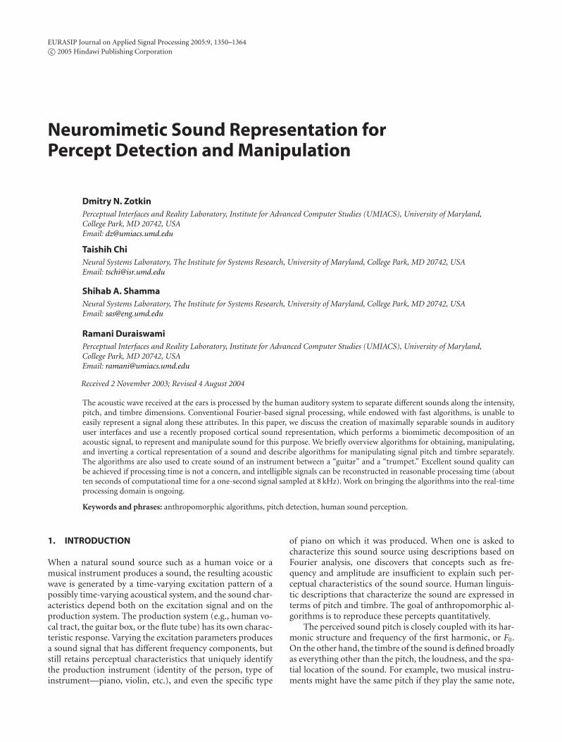
a bank of constant Q filters with some additional operationsand efficiently computes the time-frequency representationof the acoustic signal, which is called the auditory spec-trogram (Figure 2). The auditory spectrogram is invertiblethrough an iterative process (described in the next section);perceptually perfect inversion can be achieved, albeit at a verysignificant computational expense. A time slice of the spec-trogram is called the auditory spectrum.

The second processing stage mimics the action of thehigher central auditory stages (especially the primary audi-tory cortex). We provide a mathematical derivation (as pre-sented in [3]) of the cortical representation below, as well asqualitatively describe the processing.

The existence of a wide variety of neuron spectro-temporal response fields (SRTF) covering a range of fre-quency and temporal characteristics [21] suggests that theymay, as a population, perform a multiscale analysis of theirinput spectral profile. Specifically, the cortical stage estimatesthe spectral and temporal modulation content of the audi-tory spectrogram using a bank of modulation selective filtersh(t, x;ω,Ω,ϕ, θ). Each filter is tuned (Q = 1) to a combi-nation of a particular spectral modulation and a particulartemporal modulation of the incoming signal, and filters arecentered at different frequencies along the tonotopical axis.

2000

1000

500

250

125

Frequency

(Hz)

200 400 600 800 1000

Time (ms)

Figure 2: Example auditory spectrogram for the sentence “Thismovie is provided . . . ”.

These two types of modulations are defined as follows.(i) Temporal modulation, which defines how fast the sig-

nal energy is increasing or decreasing along the time axis at agiven time and frequency. It is characterized by the parame-ter ω, which is referred to as rate or velocity and is measuredin Hz, and by characteristic temporal modulation phase ϕ.

(ii) Spectral modulation, which defines how fast the sig-nal energy varies along the frequency axis at a given timeand frequency. It is characterized by the parameter Ω, whichis referred to as density or scale and is measured in cyclesper octave (CPO), and by characteristic spectral modulationphase θ.

The filters are designed for a range of rates from 2to 32Hz and scales from 0.25 to 8 CPO, which corre-sponds to the ranges of neuron spectro-temporal responsefields found in the primate brain. The impulse responsefunction for the filter h(t, x;ω,Ω,ϕ, θ) can be factored intohs(x;Ω, θ)-spectral and ht(t;ω,ϕ)-temporal parts, respec-tively. The spectral impulse response function hs(x;Ω, θ) isdefined through a phase interpolation of the spectral filterseed function u(x;Ω) with its Hilbert transform u(x;Ω), andthe temporal impulse response function is similarly definedvia the temporal filter seed function v(t;ω):

hs(x;Ω, θ) = u(x;Ω) cos θ + u(x;Ω) sin θ,

ht(t;ω,ϕ) = v(t;ω) cosϕ + v(t;ω) sinϕ.(2)

The Hilbert transform is defined as

f (x) = 1π

∫∞−∞

f (z)z − x

dz. (3)

We choose

u(x) = (1− x2)e−x

2/2, v(t) = e−t sin(2πt) (4)

1354 EURASIP Journal on Applied Signal Processing

1

0.8

0.6

0.4

0.2

0

−0.2

−0.4

−0.6

Amplitude

−1.5 −1 −0.5 0 0.5 1 1.5

Frequency (octaves)

(a)

1

0.8

0.6

0.4

0.2

0

−0.2

−0.4

−0.6

Amplitude

0 1 2 3 4 5

Time (s)

(b)

Figure 3: Tuning curves for the basis (seed) filter for the rate-scale decomposition. The seed filter is tuned to the rate of 1Hz and the scaleof 1 CPO. (a) Spectral response. (b) Temporal response.

as the functions that produce the basic seed filter tuned to ascale of 1 CPO and a rate of 1Hz. Figure 3 shows its spec-tral and temporal responses generated by functions u(x) andv(t), respectively. Differently tuned filters are obtained by di-lation or compression of the filter (4) along the spectral andtemporal axes:

u(x;Ω) = Ωu(Ωx), v(t;ω) = ωv(ωt). (5)

The response rc(t, x) of a cell c with parameters ωc, Ωc,ϕc, θc to the signal producing an auditory spectrogram y(t, x)can therefore be obtained as

rc(t, x;ωc,Ωc,ϕc, θc

) = y(t, x)⊗ h(t, x;ωc,Ωc,ϕc, θc

), (6)

where ⊗ denotes a convolution both on x and on t.An alternative representation of the filter can be derived

in the complex domain. Denote

hs(x;Ω) = u(x;Ω) + ju(x;Ω),

ht(t;ω) = v(t;ω) + jv(t;ω),(7)

where j = √−1. Convolution of y(t, x) with a downward-moving STRF obtained as hs(x;Ω)ht(t;ω) and an upward-moving SRTF obtained as hs(x;Ω)h∗t (t;ω) (where asteriskdenotes complex conjugation) results in two complex re-sponse functions:

zd(t, x;ωc,Ωc

) = y(t, x)⊗ [hs(x;Ωc)ht(t;ωc

)]= ∣∣zd(t, x;ωc,Ωc

)∣∣e jψd(t,x;ωc ,Ωc),

zu(t, x;ωc,Ωc

) = y(t, x)⊗ [hs(x;Ωc)h∗t(t;ωc

)]= ∣∣zu(t, x;ωc,Ωc

)∣∣e jψu(t,x;ωc ,Ωc),

(8)

and it can be shown [3] that

rc(t, x;ωc,Ωc,ϕc, θc

) = 12

[∣∣zd∣∣ cos (ψd − ϕc − θc)

+∣∣zu∣∣ cos (ψu + ϕc − θc

)] (9)

(the arguments of zd, zu, ψd, and ψu are omitted here forclarity). Thus, the complex wavelet transform (8) uniquelydetermines the response of a cell with parameters ωc, Ωc,ϕc, θc to the stimulus, resulting in a dimensionality reduc-tion effect in the cortical representation. In other words,knowledge of the complex-valued functions zd(t, x;ωc,Ωc)and zu(t, x;ωc,Ωc) fully specifies the six-dimensional corticalrepresentation rc(t, x;ωc,Ωc,ϕc, θc). The cortical representa-tion thus can be obtained by performing (8) which results ina four-dimensional (time, frequency, rate, and scale) hyper-cube of (complex) filter coefficients that can be manipulatedas desired and inverted back into the audio signal domain.

Essentially, the filter output is computed by a convolu-tion of its spectro-temporal impulse response (STIR) withthe input auditory spectrogram, producing a modified spec-trogram. Since the spectral and temporal cross-sections ofan STIR are typical of a bandpass impulse response in hav-ing alternating excitatory and inhibitory fields, the output ata given time-frequency position of the spectrogram is largeonly if the spectrogram modulations at that position aretuned to the rate, scale, and direction of the STIR. A map ofthe responses across the filter bank provides a unique charac-terization of the spectrogram that is sensitive to the spectralshape and dynamics over the entire stimulus.

To emphasize the features of the model that are im-portant for the current work, note that every filter in therate-scale analysis responds well to the auditory spectro-gram features that have high correlation with the filter shape.

Neuromimetic Sound Representation for Percept Manipulation 1355

0.4

0.2

0Amplitude

125 250 500 1000 2000

Frequency (Hz)

(a)

0.2

0

−0.2Amplitude

125 250 500 1000 2000

Frequency (Hz)

(b)

0.2

0

−0.2Amplitude

125 250 500 1000 2000

Frequency (Hz)

(c)

0.2

0

−0.2Amplitude

125 250 500 1000 2000

Frequency (Hz)

(d)

0.5

0

−0.5Amplitude

125 250 500 1000 2000

Frequency (Hz)

(e)

0.5

0

−0.5Amplitude

125 250 500 1000 2000

Frequency (Hz)

(f)

0.5

0

−0.5Amplitude

125 250 500 1000 2000

Frequency (Hz)

(g)

2

1.5

1

0.5

0

Amplitude

125 250 500 1000 2000

Frequency (Hz)

(h)

Figure 4: Sample scale decomposition of (h) the auditory spectrum using different scales: (a) DC, (b) 0.25, (c) 0.5, (d) 1.0, (e) 2.0,(f) 4.0, and (g) 8.0.

The filter shown in Figure 3 is tuned to the scale of 1 CPOand essentially extracts features that are of about this par-ticular width on the log-frequency axis. A scale analysis per-formed with filters of different tuning (different width) willthus decompose the spectrogram into sets of decompositioncoefficients for different scales, separating the “wide” featuresof the spectrogram from the “narrow” features. Somemanip-ulations can then be performed on parts of the decomposedspectrogram, and a modified auditory spectrogram can beobtained by inverse filtering. Similarly, rate decompositionallows for segregation of “fast” and “slow” dynamic eventsalong the temporal axis. A sample scale analysis of the audi-tory spectrogram is presented in Figure 4 (Figure 4h is theauditory spectrum, Figure 4a is the DC level of the signalwhich is necessary for the reconstruction, and the remaining6 plots show the results of processing of the given auditoryspectrum with filters of scales ranging from 0.25 to 8 CPO),and the rate analysis is similar.

Additional useful insights into the rate-scale analysis canbe obtained if we consider it as a two-dimensional wavelet

decomposition of an auditory spectrogram using a set of ba-sis functions, which are called sound ripples. The sound rip-ple is simply a spectral ripple that drifts upwards or down-wards in time at a constant velocity and is characterized bythe same two parameters—scale (density of peaks per octave)and rate (number of peaks drifting past any fixed point onthe log-frequency axis per 1-second time frame). Thus, anupward ripple with scale 1 CPO and rate 1Hz has alternat-ing peaks and valleys in its spectrum with 1 CPO periodicity,and the spectrum shifts up along the time axis, repeating it-self with 1Hz periodicity (Figure 5). If this ripple is used asan input audio signal for the cortical model, strong localizedresponse is seen at the filter with the corresponding selectiv-ity of ω = 1Hz, Ω = 1 CPO. All other basis functions areobtained by dilation (compression) of the seed-sound ripple(Figure 5) in both time and frequency. (The difference be-tween the ripples and the filters used in the cortical modelis that the seed spectro-temporal response used in corticalmodel (4) and shown in Figure 3 is local; the seed-soundripple can be obtained from it by reproducing the spatial

1356 EURASIP Journal on Applied Signal Processing

2000

1000

500

250

125

Frequency

(Hz)

0 1 2 3 4

Time (s)

Figure 5: Sound ripple at the scale of 1 CPO and the rate of 1Hz.

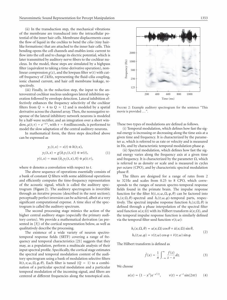
response at every octave and removing the time decay fromthe time response, andmultiscale decomposition can then beviewed as overlapping the auditory spectrogram with differ-ent sound ripples and performing local cross-correlations atvarious places over the spectrogram.) In Figure 6, we showthe result of filtering of the sample spectrogram showed ear-lier using two particular differently tuned filters, one withω = 8Hz, Ω = 0.5 CPO, and the other with ω = −2Hz,Ω = 2 CPO. It can be seen that the filter output is the highestwhen the spectrogram features match the tuning of the filterboth in rate and scale.

As such, to obtain a multiscale representation of the au-ditory spectrogram, complex filters having the “local” soundripples (5) of different rates, scales, and central frequenciesas their real parts and Hilbert transforms of these ripples astheir imaginary parts are applied to the input audio signal asa wavelet transform (8). The result of this decomposition isa four-dimensional hypercube of complex filter coefficientsthat can be modified and inverted back to the acoustic sig-nal. The phase of the coefficient shows the best-fitting direc-tion of the filter over a particular location of the auditoryspectrogram. This four-dimensional hypercube is called thecortical representation of the sound. It can be manipulatedto produce desired effects on the sound, and in the followingsections, we show some of the possible sound modifications.

In the cortical representation, two-dimensional rate-scaleslices of the hypercube reveal the features of the signal thatare most prominent at a given time. The rate-scale plotevolves in time to reflect changing ripple content of the spec-trogram. Example of rate-scale plots are shown in Figure 7where brightness of the pixel located at the intersection of

particular rate and scale values corresponds to the magni-tude of response of the filter tuned to these rate and scalevalues. For simplification of data presentation, these plotsare obtained by integration of the response magnitude overthe tonotopical axis. The first plot is a response of the cor-tical model to a single downward-moving sound ripple withω = 3Hz, Ω = 2 CPO; the best-matching filter (or, in otherwords, the “neuron” with the corresponding SRTF) respondsbest. The responses of 2Hz and 4Hz units are not equal herebecause of the cochlear filter bank asymmetry in the earlyprocessing stage. The other three plots show the evolution ofthe rate-scale response at different time instants of the sampleauditory spectrogram shown in Figure 2 (at approximately600, 720, and 1100 milliseconds, respectively); one can in-deed trace the plot time stamps back to the spectrogramand see that the spectrogram has mostly sparse downward-moving and mostly dense upward-moving features appear-ing before the 720- and 1100-millisecondmarks, respectively.The peaks in the test sentence plots are sharper in rate thanin scale, which can be explained by the integration performedover the tonotopical axis in these plots (the speech signal isunlikely to elicit significantly different rate-scale maps at dif-ferent frequencies anyway because it consists mostly of equi-spaced harmonics that can rise or fall only in unison, so therate at which the highest response is seen is not likely to dif-fer at different points on the tonotopical axis; the prevalentscale does change somewhat though due to higher numberof harmonics per octave at higher frequencies).

4. RECONSTRUCTING THE AUDIO FROM THEMODEL

After altering the cortical representation, it is necessary to re-construct the modified audio signal. Just as with the forwardpath, the reconstruction consists of two steps, correspond-ing to the central processing stage and the early processingstage. The first step is the inversion of the cortical multiscalerepresentation back to a spectrogram. It is a one-step inversewavelet transform operation because of the linear nature ofthe transform (8), which in the Fourier domain can be writ-ten as

Zd(ω,Ω;ωc,Ωc

) = Y(ω,Ω)Hs(Ω;Ωc

)Ht(ω;ωc

),

Zu(ω,Ω;ωc,Ωc

) = Y(ω,Ω)Hs(Ω;Ωc

)H∗

t

(− ω;ωc),

(10)

where capital letters signify the Fourier transforms of thefunctions determined by the corresponding lowercase letters.From (10), similar to the usual Fourier transform case, onecan write the formula for the Fourier transform of the recon-structed auditory spectrogram yr(t, x) from its decomposi-tion coefficients Zd, Zu as

Yr(ω,Ω) =∑

ωc ,ΩcZd(ω,Ω;ωc,Ωc

)H∗

t

(ω;ωc

)H∗

s

(Ω;Ωc

)+∑

ωc ,ΩcZu(ω,Ω;ωc,Ωc

)Ht(− ω;ωc

)H∗

s

(Ω;Ωc

)∑

ωc ,Ωc

∣∣Ht(ω;ωc

)Hs(Ω;Ωc

)∣∣2 +∑ωc ,Ωc

∣∣H∗t

(− ω;ωc)Hs(Ω;Ωc

)∣∣2 . (11)

Neuromimetic Sound Representation for Percept Manipulation 1357

0.5 CPO 8Hzupwards

4000

2000

1000

500

250

Frequency

(Hz)

200 600 1000Time (ms)

4000

2000

1000

500

250

Frequency

(Hz)

200 400 600 800 1000 1200Time (ms)

2 CPO 2Hzdownwards

4000

2000

1000

500

250Frequency

(Hz)

200 600 1000Time (ms)

4000

2000

1000

500

250

Frequency

(Hz)

200 400 600 800 1000 1200

Time (ms)

4000

2000

1000

500

250

Frequency

(Hz)

200 400 600 800 1000 1200

Time (ms)

Figure 6: Wavelet transform of a sample auditory spectrogram (shown in Figure 2) using two sound ripples.

Then, yr(t, x) is obtained by inverse Fourier transform ofYr(ω,Ω) and is rectified to ensure that the resulting spectro-gram is positive. The subscript r here and below refers to thereconstructed version of the signal. Excellent reconstructionquality is obtained within the effective band because of thelinear nature of involved transformations.

The second step (going from the auditory spectrogramto the acoustic wave) is a complicated task due to the non-linearity of the early auditory processing stage (nonlinearcompression and half-wave rectification), which leads to theloss of the component phase information (because the audi-tory spectrogram contains only the magnitude of each fre-quency component), and a direct reconstruction cannot beperformed. Therefore, the early auditory stage is inverted it-eratively using a convex projection algorithm adapted from[22], which takes the spectrogram as an input and recon-structs the acoustic signal that produces the spectrogramclosest to the given one.

Assume that an auditory spectrogram yr(t, x) is obtainedusing (11) after performing some manipulations in the cor-tical representation, and it is now necessary to invert it backto the acoustic signal sr(t). Observe that the analysis (first)step of the early auditory processing stage is linear and thusinvertible. If an output of the analysis step y1r(t, x) is known,the acoustic signal sr(t) can be obtained as

sr(t) =∑x

y1r(t, x)⊕ h(−t; x). (12)

The challenge is to proceed back from yr(t, x) to y1r(t, x).In the convex projection method, an iterative adaptation ofthe estimate y1r(t, x) is performed based on the differencebetween yr(t, x) and the result of the processing of y1r(t, x)through the second and third steps of the early auditory pro-cessing stage. The processing steps are listed below.

(i) Initialize the reconstructed signal s(1)r (t) by aGaussian-distributed white noise with zero mean and unitvariance. Set iteration counter k = 1.

(ii) Compute y(k)1r (t, x), y(k)2r (t, x), and y(k)r (t, x) from

s(k)r (t) using (1).

(iii) Compute the ratio r(k)(t, x) = yr(t, x)/ y(k)r (t, x).

(iv) Adjust y(k+1)1r (t, x) = r(k)(t, x) y(k)1r (t, x).

(v) Compute s(k+1)r (t) using (12). Increase k by 1.(vi) Repeat from step 2 unless the preset number of itera-

tions is reached or a certain quality criterion is met (e.g., theratio r(k)(t, x) is sufficiently close to unity everywhere).

Sample auditory spectrograms of the original and the re-constructed signals are shown later, and the reconstructionquality for the speech signal after a sufficient number of iter-ations is very good.

5. ALTERNATIVE IMPLEMENTATION OF THE EARLYAUDITORY PROCESSING STAGE

An alternative, much faster implementation of the early au-ditory processing stage was developed and can best be usedfor a fixed-pitch signal (e.g., a musical instrument tone).

1358 EURASIP Journal on Applied Signal Processing

0.25

0.5

1

2

4

8

Scale

−16 −8 −4 −2 2 4 8 16

Rate

(a)

0.25

0.5

1

2

4

8

Scale

−16 −8 −4 −2 2 4 8 16

Rate

(b)

0.25

0.5

1

2

4

8

Scale

−16 −8 −4 −2 2 4 8 16

Rate

(c)

0.25

0.5

1

2

4

8

Scale

−16 −8 −4 −2 2 4 8 16

Rate

(d)

Figure 7: Rate-scale plots of response of cortical model to different stimuli. (a) Response to 2 CPO 3Hz downward sound ripple. (b)–(d)Response at different temporal positions within the sample auditory spectrogram presented in Figure 2 (at 600, 720, and 1100 milliseconds,respectively).

In this implementation, which we will refer to as a log-Fourier transform early stage, a simple Fourier transform isused in place of the processing described by (1). We take ashort segment of the waveform s(t) at some time t( j) andperform a Fourier transform of it to obtain S( f ). The S( f )is obviously discrete with the total of L/2 points on the lin-ear frequency axis, where L is the length of the Fourier trans-form buffer. Somemappingmust be established from the lin-ear frequency axis f to the logarithmically growing tonotopi-cal axis x. We divide a tonotopical axis into segments corre-sponding to channels. Assume that the cochlear filter bankhas N channels per octave and that the lowest frequency of

interest is f0. Then, the lower x(i)l and the upper x(i)h frequency

boundaries of the ith segment are set to be

x(i)l = f02i/N , x(i)h = f02(i+1)/N . (13)

S( f ) is then remapped onto the tonotopical axis. A pointf on a linear frequency axis is said to fall into the ith seg-

ment on the tonotopical frequency axis if x(i)l < f ≤ x(i)h . Thenumber of points that falls into a segment obviously dependson the segment length, which becomes bigger for higher fre-quencies (therefore the Fourier transform of s(t) must beperformed with very high resolution and s(t) padded appro-priately to ensure that at least a few points on the f -axis fallinto the shortest segment on the x-axis). Spectral magnitudesare then averaged for all points on the f -axis that fall into thesame segment i:

yalt(t( j), x(i)

) = 1B(i)

∑x(i)l < f≤x(i)h

∣∣S( f )∣∣, (14)

where B(i) is the total number of points on f -axis that fallsinto the ith segment on x-axis (the number of terms in thesummation), and the averaging is performed for all i, gener-ating a time slice yalt(t( j), x). The process is carried out forall time segments of s(t), producing yalt(t, x), which can besubstituted for the y(t, x) computed using (1) for all furtherprocessing.

The reconstruction proceeds in an inverse manner. At ev-ery time slice t( j), a set of y(t( j), x) is remapped to the mag-nitude spectrum S( f ) on a linear frequency axis f so that

S( f ) =y(t( j), x(i)

)if for some i, x(i)l < f ≤ x(i)h ,

0 otherwise.(15)

At this point, the magnitude information is set cor-rectly in S( f ) to perform inverse Fourier transform but thephase information is lost. Direct one-step reconstructionfrom S( f ) is much faster than the iterative convex projectionmethod described above but produces unacceptable resultswith clicks and strong interfering noise at the frequency cor-responding to the processing window length. Processing thesignal in heavily overlapping segments with gradual fade-inand fade-out windowing functions somewhat improves theresults but the reconstruction quality is still significantly be-low the quality achieved using the iterative projection algo-rithm described in Section 4.

One way to recover the phase information and to useone-step reconstruction of s(t) from magnitude spectrumS( f ) is to save the bin phases of the forward-pass Fouriertransform and later impose them on S( f ) after it is recon-

Neuromimetic Sound Representation for Percept Manipulation 1359

structed from the (altered) cortical representation. Signifi-cantly better continuity of the signal is obtained in this man-ner. However, it seems that the saved phases carry the imprintof the original pitch of the signal, which produces undesir-able effects if the processing goal is to perform a pitch shift.

However, the negative effect of the phase set carrying thepitch imprint can be reversed and used for good simply bygenerating the set of bin phases that corresponds to a desiredpitch and imposing them on S( f ). Of course the knowledgeof the signal pitch is required in this case, which is not al-ways easy to obtain. We have used this technique in perform-ing timbre-preserving pitch shift of musical instrument noteswhere the exact original pitch F0 (and therefore the exactshifted pitch F′0) is known. To obtain the set of phases cor-responding to the pitch F′0, we generate, in the time domain,a pulse train of frequency F′0 and take its Fourier transformwith the same window length as used in the processing ofS( f ). The bin phases of the Fourier transform of the pulsetrain are then imposed on the magnitude spectrum S( f ) ob-tained in (15). In this manner, very good results are obtainedat reconstructingmusical tones of a fixed frequency; it shouldbe noted that such reconstruction is not handled well by theiterative convex projection method described above—the re-constructed signal is not a pure tone but rather constantlyjitters up and down, preventing any musical perception, pre-sumably because the time slices of s(t) are treated indepen-dently by convex projection algorithm, which does not at-tempt to match signal features from adjacent time frames.

Nevertheless, speech reconstruction is handled better bythe significantly slower convex projection algorithm, becauseit is not clear how to select F′0 to generate the phase set.If the log-Fourier transform early stage can be applied tothe speech signals, significant processing speed-up can beachieved. A promising idea is to employ a pitch detectionmechanism at each frame of s(t) to detect F0, to compute F′0,and to impose F′0-consistent phases on S( f ) to enable one-step recovery of s(t), which is the subject of ongoing work.

6. RECONSTRUCTIONQUALITY

It is important to do an objective evaluation of the recon-structed sound quality. The second (central) stage of the cor-tical model processing is perfectly invertible because of thelinear nature of the wavelet transformations involved, and itis the first (early) stage that presents difficulties for the in-version because of the phase information loss in the pro-cessing. Given the modified auditory spectrogram yr(t, x),the convex projection algorithm described above tries to syn-thesize the intermediate result y1r(t, x) that, when processedthrough the two remaining steps of the early auditory stage,yields yr(t, x) that is as close as possible to yr(t, x). The wave-form sr(t) can then be directly reconstructed from y1r(t, x).The reconstruction error measure E is defined as the averagerelative magnitude difference between the target yr(t, x) andthe candidate yr(t, x):

E = 1B

∑i, j

∣∣ yr(t( j), x(i))− yr(t( j), x(i)

)∣∣yr(t( j), x(i)

) , (16)

where B is the total number of terms in the summation. Dur-ing the iterative update of y1r(t, x), the error E does not dropmonotonically; instead, the lower the error, the higher thechance that the next iteration actually increases the error, inwhich case the newly computed y1r(t, x) should be discardedand a new iteration should be started from the best previ-ously found y1r(t, x).

In practical tests, it was found that the error E dropsquickly to units of percents, and any further improvementrequires very significant computational expense. For the pur-poses of illustration, we took the 1200-milliseconds auditoryspectrogram (Figure 2) and ran the convex projection algo-rithm on it. It takes about 2 seconds to execute one algorithmiteration on a 1.7GHz Pentium computer. In this sample run,the error after 20, 200, and 2000 iterations was found to be4.73%, 1.60%, and 1.08%, respectively, which is representa-tive of the general behavior observed in many experiments.

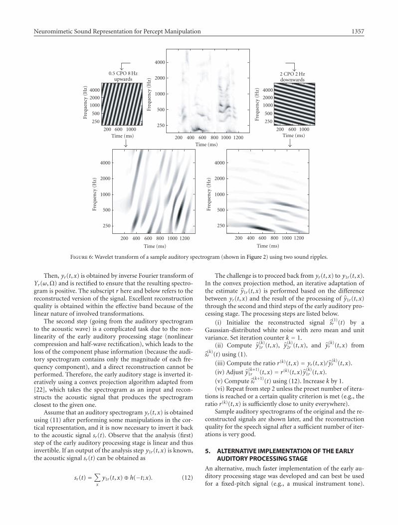
In Figure 8a, the original waveform s(t) and its corre-sponding auditory spectrogram y(t, x) from Figure 2 areplotted. The auditory spectrogram y(t, x) is used as an in-put yr(t, x) to the convex projection algorithm, which, in200 iterations, reconstructs the waveform sr(t) shown in thetop plot of Figure 8b. The spectrogram yr(t, x) correspond-ing to the reconstructed waveform is also shown in the bot-tom plot of Figure 8b. Because the reconstruction algorithmattempts to synthesize a waveform sr(t) such that its spec-trogram yr(t, x) is equal to yr(t, x), it can be expected thatthe spectrograms of the original and of the reconstructedwaveforms would match. This is indeed the case in Figure 8,but the fine waveform structure is different in the original(Figure 8a) and in the reconstruction (Figure 8b), with no-ticeably less periodicity in some segments. However, it canbe argued that because the original and the reconstructedwaveforms produce the same results when processed throughthe early auditory processing stage, the perception of theseshould be nearly identical, which is indeed the case when thesounds are played to the human ear. Slight distortions areheard in the reconstructed waveform, but the sound is clearand intelligible. Increasing the number of iterations furtherdecreases distortions; when the error drops to about 0.5%(tens of thousands of iterations), the signal is almost indis-tinguishable from the original.

We also compared the quality of the reconstructed signalwith the quality of sound produced by existing pitch modifi-cation and sound morphing techniques. In [5], spectrogrammodeling with MFCC coefficients plus residue spectrogramand iterative reconstruction process are used for sound mor-phing, and short morphing examples for voiced sounds areavailable for listening in the online version of the same pa-per. Book [7] also contains (among many other examples)some audio samples derived using algorithms that are rele-vant to our work and are targeted for the same applicationareas as we are considering, in particular, samples of cross-synthesis between the musical tone and the voice using chan-nel vocoder and resynthesis of speech and musical tones us-ing LPC with residual as an excitation signal and LPC withpulse train as an excitation signal. In our opinion, the signalquality we achieve is comparable to the quality of the relevant

1360 EURASIP Journal on Applied Signal Processing

2000

1000

500

250

125

Frequency

(Hz)

200 400 600 800 1000

Time (ms)

(a)

2000

1000

500

250

125

Frequency

(Hz)

200 400 600 800 1000

Time (ms)

(b)

Figure 8: (a) Original waveform and corresponding spectrogram. (b) Reconstructed waveform and corresponding spectrogram after 200iterations.

samples presented in these references, although the soundprocessing through a cortical representation is significantlyslower than the algorithms presented in [5, 6, 7].

In summary, it can be concluded that reasonable qual-ity of the reconstructed signal can be achieved in reasonabletime, such as ten seconds or so of computational time per onesecond of a signal sampled at 8 kHz (although the iterativealgorithm is not suitable for the real-time processing). If un-limited time (few hours) is allowed for processing, very goodsignal quality is achieved. The possibility of iterative signalreconstruction in real time is an open question and work inthis area is continuing.

7. TIMBRE-PRESERVING PITCHMANIPULATIONS

For speech and musical instruments, timbre is conveyed bythe spectral envelope, whereas pitch is mostly conveyed bythe harmonic structure, or harmonic peaks. This biologicallybased analysis is in the spirit of the cepstral analysis used inspeech [23], except that the Fourier-like transformation inthe auditory system is carried out in a local fashion usingkernels of different scales. The cortical decomposition is ex-pressed in the complex domain, with the coefficient magni-tude being the measure of the local bandwidth of the spec-trum and the coefficient phase being the measure of the lo-cal symmetry at each bandwidth. Finally, just as it is the casewith cepstral coefficients, the spectral envelope varies slowly.In contrast, the harmonic peaks are only visible at high res-olution. Consequently, timbre and pitch occupy different re-gions in the multiscale representation. If X is the auditoryspectrum of a given data frame, with the length N equal tothe number of filters in the cochlear filter bank, and the de-composition is performed overM scales, then the matrix S ofthe scale decomposition ofX hasM rows, one per scale value,and N columns. If the first (top) row of S contains the de-composition over the finest scale and theMth (bottom) row

is the coarsest one, then the components of S in the upperleft triangle can be associated with pitch, whereas the rest ofthe components can be associated with timbre information[24]. In Figure 9, sample plot of the scale decomposition ofthe auditory spectrum is shown. (Please note that this is ascale versus tonotopical frequency plot rather than scale-rateplot; all rate decomposition coefficients carry timbre infor-mation.) The brightness of a pixel corresponds to the mag-nitude of the decomposition coefficient, whereas the rela-tive length and the direction of the arrow at the pixel showthe coefficient phase. The white solid diagonal line shown inFigure 9 roughly separates timbre and pitch information inthe cortical representation. The coefficients that lie above thisline carry primarily pitch information, and the rest can be as-sociated with timbre.

To control pitch and timbre separately, we apply modi-fications at appropriate locations in the cortical representa-tion matrix and invert the cortical representation back to thespectrogram. Thus, to shift the pitch while holding the tim-bre fixed, we compute the cortical multiscale representationof the entire sound, shift (along the frequency axis) the trian-gular part of every time slice of the hypercube that holds thepitch information while keeping the timbre information in-tact, and invert the result. To modify the timbre keeping thepitch intact, we do the opposite. It is also possible to splicethe pitch and the timbre information from two speakers, orfrom a speaker and a musical instrument. The result after in-version back to the sound is a “musical” voice that sings theutterance (or a “talking” musical instrument).

We express the timbre-preserving pitch shift algorithm inmathematical terms. The cortical representation consists of aset of complex coefficients zu(t, x;ωc,Ωc) and zd(t, x;ωc,Ωc).In the actual decomposition, the values of t, x, ωc, and Ωc

are discrete, and the cortical representation of a sound is justa four-dimensional hypercube of complex coefficients Zi, j,k,l.We agree that the first index i corresponds to the time axis,

Neuromimetic Sound Representation for Percept Manipulation 1361

8.0

4.0

2.0

1.0

0.5

0.25

Scales

250 500 1000 2000 4000

Frequency (Hz)

Figure 9: Plot of the sample auditory spectrum scale decomposi-tion matrix. The brightness of the pixel corresponds to the magni-tude of the decomposition coefficient, whereas the relative lengthand the direction of the arrow at the pixel show the coefficientphase. Upper triangle of the matrix of coefficients (above the solidwhite line) contains information about the pitch of the signal. Thelower triangle contains information about the timbre.

the second index j corresponds to the frequency axis, thethird index k corresponds to the scale axis, and the fourthindex l corresponds to the rate axis. Index j varies from 1 toN , whereN is the number of filters in the cochlear filter bank,index k varies from 1 toM (in order of scale increase), whereM is the number of scales, and, finally, index l varies from 1to 2L, where L is the number of rates (zd and zu are juxta-posed in Zi, j,k,l matrix as pictured on the horizontal axis inFigure 7: l = 1 corresponds to zd with the highest rate, l = 2to zd with the next lower rate, l = L to zd with the lowest rate,l = L+1 to zu with the lowest rate, l = L+2 to zu with the nexthigher rate, and l = 2L to zu with the highest rate; this partic-ular order is not critical for the pitch modifications describedbelow as they do not depend on it). Then, the coefficient isassumed to carry pitch information if it lies above the diago-nal shown in Figure 9 (i.e., if (M−k)/ j > (M−1)/N), and toshift the pitch up by q channels, we fill the matrix Z∗i, j,k,l withthe coefficients of matrix Zi, j,k,l as follows:

Z∗i, j,k,l = Zi, j,k,l, j < jb,

Z∗i, j,k,l = Zj, jb ,k,l, jb ≤ j < jb + q,

Z∗i, j,k,l = Zi, j−q,k,l, jb + q ≤ j,

(17)

where jb = (M−k)N/(M−1) rounded to the nearest positiveinteger (note that jb depends on k and therefore is differentin different hyperslices of the matrix that have different val-ues of k). The similar procedure shifts the pitch down by qchannels:

Z∗i, j,k,l = Zi, j,k,l, j < jb,

Z∗i, j,k,l = Zi, j+q,k,l, jb ≤ j < N − q,

Z∗i, j,k,l = Zi,N ,k,l, jb ≤ j, N − q ≤ j.

(18)

0−10−20−30−40−50−60M

agnitude

(dB)

125 250 500 1000 2000

Frequency (Hz)

(a)

0−10−20−30−40−50−60M

agnitude

(dB)

125 250 500 1000 2000

Frequency (Hz)

(b)

Figure 10: Spectrum of a speech signal (a) before and (b) after pitchshift. Note that the spectral envelope is filled with the new set ofharmonics.

Finally, to splice the pitch of the signal S1 with the tim-bre of the signal S2, we compose Z∗ from two correspondingcortical decompositions Z1 and Z2, taking the elements forwhich (M − k)/ j > (M − 1)/N from Z1 and all other onesfrom Z2. Inversion of Z∗ back to the waveform gives us thedesired result.

We show one-pitch shift example here and refer theinterested reader to http://www.isr.umd.edu/CAAR/ andhttp://www.umiacs.umd.edu/labs/pirl/NPDM/ for the actualsounds used in this example, and for more samples. Weuse the above-described algorithm to perform a timbre-preserving pitch shift of a speech signal. The cochlear modelhas 128 filters with 24 filters per octave, covering 5(1/3) oc-taves along the frequency axis. The cortical representation ismodified using (18) to achieve the desired pitch modifica-tion and then inverted using the reconstruction proceduredescribed in Section 4, resulting in a pitch-scaled version ofthe original signal. In Figure 10, we show plots of the spec-trum of the original signal and of the signal having the pitchshifted down by 8 channels (one third of an octave) at a fixedpoint in time. The pitches of the original and of the modi-fied signals are 140Hz and 111Hz, respectively. It can be seenfrom the plots that the signal spectral envelope is preservedand that the speech formants are kept at their original loca-tions, but a new set of harmonics is introduced.

The algorithm is sufficiently fast to be used in real time ifa log-Fourier transform early stage (described in Section 5)is substituted for a cochlear filter bank to eliminate the needfor an iterative inversion process. Additionally, it is not neces-sary to compute the full cortical representation of the soundto do timbre-preserving pitch shifts. It is enough to performonly scale decomposition for every time frame of the audi-tory spectrogram because shifts are done along the frequency

1362 EURASIP Journal on Applied Signal Processing

0.5

0

−0.5

Amplitude

0 0.25 0.5 0.75 1.0 1.25

Time (s)

0

−30

−60

−90

Magnitude

(dB)

0 2000 4000 6000 8000

Frequency (Hz)

0.5

0

−0.5

Amplitude

0 0.25 0.5 0.75 1.0 1.25

Time (s)

0

−30

−60

−90

Magnitude

(dB)

0 2000 4000 6000 8000

Frequency (Hz)

0.5

0

−0.5

Amplitude

0 0.25 0.5 0.75 1.0 1.25

Time (s)

0

−30

−60

Magnitude

(dB)

0 2000 4000 6000 8000

Frequency (Hz)

Figure 11: (Left column) Waveform plots and (right column) spectrum plots for guitar (top plots), trumpet (middle plots), and newinstrument (bottom plots).

axis and can be performed in each time slice of the hypercubeindependently; thus, the rate decomposition is unnecessary.We have used the pitch-shift algorithm in a small-scale studyin an attempt to generate maximally separable sounds to im-prove simultaneous eligibility of multiple competing mes-sages [19]; it was found that the pitch separation does im-prove the perceptual separability of sounds and the recogni-tion rate. Also, we have used the algorithm to generate, fromone note of a given frequency, other notes of a newly createdmusical instrument that has the timbre characteristics of twoexisting instruments. This application is described in moredetails in the following section.

8. TIMBREMANIPULATIONS

Timbre of the audio signal is conveyed both by the spec-tral envelope and by the signal dynamics. Spectral envelopeis represented in the cortical representation by the lowerright triangle of the scale decomposition coefficients andcan be manipulated by modifying these. Sound dynamicsis captured by the rate decomposition. Selective modifica-tions to enhance or diminish the contributions of compo-nents of a certain rate can change the dynamic properties

of the sound. As an illustration, and as an example ofinformation separation across the cells of different rates, wesynthesize a few sound samples using simple modificationsto make the sound either abrupt or slurred. One such sim-ple modification is to zero out the cortical representation de-composition coefficients that correspond to the “fast” cells,creating the impression of a low-intelligibility sound in anextremely reverberant environment; the other one is to re-move “slow” cells, obtaining an abrupt sound in an ane-choic environment (see http://www.isr.umd.edu/CAAR/ andhttp://www.umiacs.umd.edu/labs/pirl/NPDM/ for the actualsound samples where the decomposition was performed overthe rates of 2, 4, 8, and 16Hz; from these, “slow” rates are 2and 4Hz and “fast” rates are 8 and 16Hz). It might be pos-sible to use such modifications in sonification (e.g., by map-ping some physical parameter to the amount of simulatedreverberation and by manipulating the perceived reverbera-tion time by gradual decrease or increase of contribution of“slow” components) or in audio user interfaces in general.Similarly, in the musical synthesis, playback rate and onsetand decay ratio can be modified with shifts along the rateaxis while preserving the pitch.

Neuromimetic Sound Representation for Percept Manipulation 1363

0

−30−60

Magnitude

(dB)

0 1000 2000 3000 4000 5000 6000 7000 8000

Frequency (Hz)

(a)

0

−30−60

Magnitude

(dB)

0 1000 2000 3000 4000 5000 6000 7000 8000

Frequency (Hz)

(b)

0

−30−60

Magnitude

(dB)

0 1000 2000 3000 4000 5000 6000 7000 8000

Frequency (Hz)

(c)

Figure 12: Spectrum of the new instrument playing (a) D#3, (b)C3, and (c) G2.

To show the ease with which timbre manipulation can bedone using the cortical representation, we performed a tim-bre interpolation between twomusical instruments to obtaina new in between synthetic instrument, which has both thespectral shape and the temporal spectral modulations (on-set and decay ratio) that lie between the two original instru-ments. The two instruments selected were the guitarWgC#3,and the trumpet, WtC#3, playing the same note (C#3). Therate-scale decomposition of a short (1.5 seconds) instrumentsample was performed and the geometric average of the com-plex coefficients in the cortical representations of these twoinstrument samples was computed and was converted backto the sound wave to obtain the new instrument sound sam-ple WnC#3. The behavior of the new instrument along thetime axis is intermediate between two original ones, and thespectrum shape is also an average between two original in-struments (Figure 11).

After the timbre interpolation, the synthesized instru-ment can only play the same note as the original ones. To syn-thesize other notes, we use the timbre-preserving pitch shiftalgorithm (Section 7) on the waveform WnC#3 obtained bythe timbre interpolation (third waveform in Figure 11) as aninput. Figure 12 shows the spectrum of the new instrumentfor three different newly generated notes—D#3, C3, and G2.It can be seen that the spectral envelope is the same in allthree plots (and is the same as the spectral envelope of theWnC#3), but this envelope is filled with different sets of har-monics for different notes. For this synthesis, a log-Fouriertransform early stage with pulse-train phase imprinting

(Section 5) was used, as it is ideally suited for the task. A fewsamples of music made with the new instrument are availableat http://www.umiacs.umd.edu/labs/pirl/NPDM/.

9. SUMMARY AND CONCLUSIONS

We developed and tested simple yet powerful algorithmsfor performing independent modifications of the pitch andthe timbre of an audio signal and for performing interpola-tion between sound samples. These algorithms constitute anew application of the cortical representation of the sound[3], which extracts the perceptually important audio featuressimulating the processing believed to occur in auditory path-ways in primates and thus can be used for making soundmodifications tuned for and targeted to the ways the humannervous system processes information. We obtained promis-ing results and are using these algorithms in ongoing devel-opment of auditory user interfaces.

ACKNOWLEDGMENTS

Partial support of ONR Grant N000140110571, NSF GrantIBN-0097975, and NSF Award IIS-0205271 is gratefully ac-knowledged. This paper is an extended version of paper [1].

REFERENCES

[1] D. N. Zotkin, S. A. Shamma, P. Ru, R. Duraiswami, and L. S.Davis, “Pitch and timbre manipulations using cortical repre-sentation of sound,” in Proc. IEEE Int. Conf. Acoustics, Speech,Signal Processing (ICASSP ’03), vol. 5, pp. 517–520, HongKong, China, April 2003, reprinted in Proc. ICME ’03, Bal-timore, Md, USA, July 2003, vol. 3, pp. 381–384, because ofthe cancellation of ICASSP ’03 conference meeting.

[2] M. Elhilali, T. Chi, and S. A. Shamma, “A spectro-temporalmodulation index (STMI) for assessment of speech intelli-gibility,” Speech Communication, vol. 41, no. 2, pp. 331–348,2003.

[3] T. Chi, P. Ru, and S. A. Shamma, “Multiresolution spec-trotemporal analysis of complex sounds,” to appear in Journalof the Acoustical Society of America.

[4] T. Chi, Y. Gao, M. C. Guyton, P. Ru, and S. A. Shamma,“Spectro-temporal modulation transfer functions and speechintelligibility,” Journal of the Acoustical Society of America,vol. 106, no. 5, pp. 2719–2732, 1999.

[5] M. Slaney, M. Covell, and B. Lassiter, “Automatic audio mor-phing,” in Proc. IEEE Int. Conf. Acoustics, Speech, Signal Pro-cessing (ICASSP ’96), vol. 2, pp. 1001–1004, Atlanta, Ga, USA,May 1996.

[6] X. Serra, “Musical soundmodeling with sinusoids plus noise,”in Musical Signal Processing, G. D. Poli, A. Picialli, S. T. Pope,and C. Roads, Eds., Swets & Zeitlinger Publishers, Lisse, TheNetherlands, 1997.

[7] P. R. Cook, Real Sound Synthesis for Interactive Applications,A. K. Peters, Natick, Mass, USA, 2002.

[8] S. Barrass, Sculpting a Sound Space with Information Prop-erties: Organized Sound, Cambridge University Press, Cam-bridge, UK, 1996.

[9] G. Kramer, B. Walker, T. Bonebright, et al. “Sonifica-tion report: Status of the field and research agenda,”prepared for NSF by members of the ICAD, 1997,http://www.icad.org/websiteV2.0/References/nsf.html.

1364 EURASIP Journal on Applied Signal Processing

[10] S. Bly, “Multivariate data mapping,” in Proc. Auditory Display:Sonification, Audification, and Auditory Interfaces, G. Kramer,Ed., vol. 18 of Santa Fe Institute Studies in the Sciences ofComplexity, pp. 405–416, Addison Wesley, Reading, Mass,USA, 1994.

[11] D. N. Zotkin, R. Duraiswami, and L. S. Davis, “Rendering lo-calized spatial audio in a virtual auditory space,” IEEE Trans.Multimedia, vol. 6, no. 4, pp. 553–564, 2004.

[12] D. S. Brungart, “Informational and energetic masking effectsin the perception of two simultaneous talkers,” Journal of theAcoustical Society of America, vol. 109, no. 3, pp. 1101–1109,2001.

[13] C. J. Darwin and R. W. Hukin, “Effects of reverberation onspatial, prosodic, and vocal-tract size cues to selective atten-tion,” Journal of the Acoustical Society of America, vol. 108,no. 1, pp. 335–342, 2000.

[14] C. J. Darwin and R. W. Hukin, “Effectiveness of spatial cues,prosody, and talker characteristics in selective attention,” Jour-nal of the Acoustical Society of America, vol. 107, no. 2, pp. 970–977, 2000.

[15] M. L. Hawley, R. Y. Litovsky, and H. S. Colburn, “Speech in-telligibility and localization in a multi-source environment,”Journal of the Acoustical Society of America, vol. 105, no. 6,pp. 3436–3448, 1999.

[16] W. A. Yost, R. H. Dye Jr., and S. Sheft, “A simulated cocktailparty with up to three sound sources,” Perception and Psy-chophysics, vol. 58, no. 7, pp. 1026–1036, 1996.

[17] B. Arons, “A review of the cocktail party effect,” Journal of theAmerican Voice I/O Society, vol. 12, pp. 35–50, 1992.

[18] P. F. Assmann, “Fundamental frequency and the intelligibil-ity of competing voices,” in Proc. 14th International Congressof Phonetic Sciences, pp. 179–182, San Francisco, Calif, USA,August 1999.

[19] N. Mesgarani, S. A. Shamma, K. W. Grant, and R. Du-raiswami, “Augmented intelligibility in simultaneous multi-talker environments,” in Proc. International Conference on Au-ditory Display (ICAD ’03), pp. 71–74, Boston, Mass, USA, July2003.

[20] A. S. Bregman, Auditory Scene Analysis: The Perceptual Orga-nization of Sound, MIT Press, Cambridge, Mass, USA, 1991.

[21] N. Kowalski, D. Depireux, and S. A. Shamma, “Analysis of dy-namic spectra in ferret primary auditory cortex. I. Character-istics of single-unit responses to moving ripple spectra,” Jour-nal of Neurophysiology, vol. 76, no. 5, pp. 3503–3523, 1996.

[22] X. Yang, K. Wang, and S. A. Shamma, “Auditory representa-tions of acoustic signals,” IEEE Trans. Inform. Theory, vol. 38,no. 2, pp. 824–839, 1992.

[23] F. Jelinek, Statistical Methods for Speech Recognition, MITPress, Cambridge, Mass, USA, 1998.

[24] R. Lyon and S. A. Shamma, “Auditory representations of tim-bre and pitch,” in Auditory Computations, vol. 6 of SpringerHandbook of Auditory Research, pp. 221–270, Springer-Verlag,New York, NY, USA, 1996.

Dmitry N. Zotkin was born in Moscow,Russia, in 1973. He received a combinedB.S./M.S. degree in applied mathematicsand physics from the Moscow Instituteof Physics and Technology, Dolgoprudny,Moscow Region, Russia, in 1996, and re-ceived the M.S. and Ph.D. degrees in com-puter science from the University of Mary-land, College Park, USA, in 1999 and 2002,respectively. Dr. Zotkin is currently an

Assistant Research Scientist at the Perceptual Interfaces and RealityLaboratory, Institute for Advanced Computer Studies (UMIACS),University ofMaryland, College Park. His current research interestsare in multichannel signal processing for tracking and multimedia.He is also working in the general area of spatial audio, includingvirtual auditory scene synthesis, customizable virtual auditory dis-plays, perceptual processing interfaces, and associated problems.

Taishih Chi received the B.S. degree fromNational Taiwan University, Taiwan, in1992, and the M.S. and Ph.D. degrees fromthe University of Maryland, College Park,in 1997 and 2003, respectively, all in elec-trical engineering. From 1994 to 1996, hewas a Graduate School Fellow at the Uni-versity of Maryland. From 1996 to 2003, hewas a Research Assistant at the Institute forSystems Research, University of Maryland.Since June 2003, he has been a Research Associate at the Universityof Maryland. His research interests are in neuromorphic auditorymodeling, soft computing, and speech analysis.

Shihab A. Shamma obtained his Ph.D. de-gree in electrical engineering from StanfordUniversity in 1980. He joined the Depart-ment of Electrical Engineering, the Univer-sity of Maryland, in 1984, where his re-search has dealt with issues in computa-tional neuroscience and the development ofmicrosensor systems for experimental re-search and neural prostheses. His primaryfocus has been on uncovering the compu-tational principles underlying the processing and recognition ofcomplex sounds (speech and music) in the auditory system, andthe relationship between auditory and visual processing. Other re-search interests include the development of photolithographic mi-croelectrode arrays for recording and stimulation of neural signals,VLSI implementations of auditory processing algorithms, and de-velopment of algorithms for the detection, classification, and anal-ysis of neural activity from multiple simultaneous sources.

Ramani Duraiswami is a member of thefaculty in the Department of ComputerScience and in the Institute for AdvancedComputer Studies (UMIACS), the Univer-sity of Maryland, College Park. He is the Di-rector of the Perceptual Interfaces and Re-ality Laboratory there. Dr. Duraiswami ob-tained the B.Tech. degree in mechanical en-gineering from IIT Bombay in 1985, and aPh.D. degree inmechanical engineering andapplied mathematics from the Johns Hopkins University in 1991.His research interests are broad and currently include spatial au-dio, virtual environments, microphone arrays, computer vision,statistical machine learning, fast multipole methods, and integralequations.