neural-network control of nonaffine nonlinear system with zero

900 IEEE TRANSACTIONS ON NEURAL NETWORKS, VOL. 14, NO. 4, JULY 2003

Neural-Network Control of Nonaffine NonlinearSystem With Zero Dynamics by State and

Output FeedbackShuzhi Sam Ge, Senior Member, IEEE,and Jin Zhang

Abstract—This paper focuses on adaptive control of non-affine nonlinear systems with zero dynamics using multilayerneural networks. Through neural network approximation,state feedback control is firstly investigated for nonaffinesingle-input–single-output (SISO) systems. By using a high gainobserver to reconstruct the system states, an extension is madeto output feedback neural-network control of nonaffine systems,whose states and time derivatives of the output are unavailable.It is shown that output tracking errors converge to adjustableneighborhoods of the origin for both state feedback and outputfeedback control.

Index Terms—High-gain observer, neural networks, nonaffinesystem, output feedback control, zero dynamics.

I. INTRODUCTION

I N RECENT YEARS, control system design for complexnonlinear systems has attracted much attention. Many re-

markable results in this area have been obtained, including feed-back linearization techniques [1], adaptive backstepping design[2], neural-network (NN) control [3], [4] and fuzzy logic con-trol [5]. Most of these researches are conducted for systems inaffine form. Based on differential geometry theory which is avery useful analytical tool for nonlinear control system design,several adaptive schemes have been developed in dealing withthe problem of parametric uncertainties [6], [7] for affine non-linear systems. But there are some practical systems, such aschemical reactions [8], their input variables cannot be expressedin an affine form. Because the input does not appear linearly,which makes the direct feedback linearization difficult, controlsystem design for nonaffine nonlinear systems are not an easytask.

Zero dynamics exist in many practical systems, includingisothermal continuous stirred tank reactors (CSTR) [9], field-controlled dc motors [10], controlled van der Pol equation [11],aircraft trajectory tracking control [12], and others. It is nec-essary to investigate their influence on control system design.Zero dynamics play an important role in the areas of modeling,analysis, and control of linear and nonlinear systems. For linearsystems, internal dynamics are defined to be the states that arenot observable after a Lie derivative coordinate transformation[13]. By keeping the system output at zero, we obtain the zero

Manuscript received June 11, 2001; revised September 12, 2002.The authors are with the Department of Electrical Engineering, Na-

tional University of Singapore, Singapore 117576, Singapore (e-mail:[email protected]).

Digital Object Identifier 10.1109/TNN.2003.813823

dynamics. The stability of the internal dynamics is simply de-termined by the locations of the zeros, and the stability of zerodynamics implies the global stability of the internal dynamics.For nonlinear systems, intuitions for linear systems are used todefine zero dynamics of nonlinear system. They are defined tobe the internal dynamics of the systems when the system outputis kept at zero. However, unlike the linear case, no results on theglobal stability or even large range stability can be drawn forthe internal dynamics of nonlinear systems and only local sta-bility is guaranteed for the internal dynamics even if the zero dy-namics are globally exponentially stable. The zero dynamics ofnonlinear system are an intrinsic feature of a nonlinear system,which do not depend on the choice of the control law or the de-sired trajectories when they are represented in a normal formwhere the control input does not explicitly appear in the in-ternal dynamics [11], [13]. But sometimes it is difficult to ob-tain the normal form because of the difficulty in constructingthe transformation functions. With control inputappears inthe internal dynamics, different forms may exist [1]. It is notdifficult to arrive at similar conclusions and properties as thosein a normal form. Much research work has been carried out forsystems with zero dynamics [14]–[18].

Recently, NNs have been made particularly attractive andpromising for applications to modeling and control of nonlinearsystems, owing to its universal approximation abilities, learningand adaptation, parallel distributed abilities. The feasibility ofapplying NNs to model unknown functions in dynamic systemshas been demonstrated in several studies [19], [20]. From theseworks, it has been shown that for stable and efficient onlinecontrol using the backpropagation (BP) learning algorithm, theidentification must be sufficiently accurate before control actioncould be initiated. In practical control applications, it is desir-able to have systematic methods of ensuring the stability, ro-bustness, and performance properties of the overall system. Re-cently, several good NN control approaches have been proposedbased on Lyapunov analysis [3], [4], [21], [22]. One main ad-vantage of these schemes is that the adaptive laws are derivedbased on Lyapunov synthesis, therefore, guarantee the stabilityof the closed-loop systems. However, they can only be appliedto relatively simple classes of nonlinear plants in affine forms[3], [4]. For NN control system design of general nonlinear sys-tems, several researchers have suggested to use NNs as emula-tors of inverse systems. The main idea is that for a system witha finite relative degree, the mapping between a system input andthe system output is one-to-one, thus allowing the constructionof a “left-inverse” of the nonlinear system using NN. Using the

1045-9227/03$17.00 © 2003 IEEE

GE AND ZHANG: NEURAL-NETWORK CONTROL OF NONAFFINE NONLINEAR SYSTEM 901

implicit function theory, the NN control methods proposed in[20], [23] have been used to emulate the “inverse controller”to achieve the desired control objectives, though no rigorousproof was given in [23]. Based on this idea, adaptive control withrigorous analysis has been investigated for nonaffine nonlinearsystem by using multilayer NNs in [24], [25] and was appliedin [8]. None of the above works considered the zero dynamics,though it plays an important role in nonlinear system control.

In this paper, we are interested in how to control thesingle-input–single-output (SISO) nonaffine nonlinear systemwith zero dynamics using multilayer NNs. The problem is notonly academically challenging but also of practical interest.Academically, it is very much involved and tedious to extendthe results in [24], [25] for nonaffine nonlinear SISO systemto nonaffine nonlinear system with zero dynamics. In practice,there are indeed systems that have zero dynamics which includecertain types of CSTR systems [9], field-controlled dc motorsystems [10] and others. In this paper, based on the implicitfunction theorem, multilayer NNs are used to approximatethe implicit desired feedback control. For the system’s zerodynamics, we first assume that the zero dynamics are min-imum-phase, i.e., zero dynamics are exponentially stable, thenunder the Lipschitz condition assumption, by using converseLyapunov theorem, we can show that the system’s internalstates do remain in a compact set.

The main contributions of this paper are: 1) the proof of theexistence of implicit desired feedback control based on implicitfunction theorem; 2) state feedback control for nonaffine non-linear system using NNs; and 3) observer-based NN output con-trol for nonaffine nonlinear system. It should be noted that, al-though the control schemes are developed for nonaffine systemswith zero dynamics, they also can be applied to affine systemwithout zero dynamics, affine system with zero dynamics andnonaffine system without zero dynamics, assuming all the as-sumptions are satisfied. There is no doubt these kinds of sys-tems cover a wide class of practical processes.

This paper is organized as follows. In Section II, by usingLie derivative, the general form of the SISO nonaffine system istransformed into a normal form in the new coordinates. Then theexistence of implicit desired feedback control (IDFC) is provedunder some mild assumptions. The state feedback control andthe output feedback control are presented in Sections III andIV, respectively. A practical CSTR process simulation shows theeffectiveness of the proposed control methods.

II. PROBLEM STATEMENT

Consider SISO nonaffine system

(1)

where is the state vector, is the input, andis the output. The mapping is a partiallyunknown smooth vector field and is a partiallyunknown smooth function, the degree of uncertainties will beexplained later. The control objective is to design a controllersuch that the system outputfollows the desired trajectory .The main difficulty of this control problem is that the system

input does not appear linearly, which makes the direct feed-back linearization difficult/impossible.

A. System Transform via Lie Derivative

Let denote the Lie derivative of the function withrespect to the vector field as

Higher order Lie derivatives can be defined recursively as, .

Let and be two compact sets such thatand . System (1) is said to have a strong relative

degree in if there exists a positive integersuch that

(2)

for all [26].Assumption 2.1:System (1) possesses a strong relative de-

gree , .Define , . Under Assumption

2.1, it was shown in [1], [6] that there exist other functions, which are independent of, such that the

mapping

(3)

has a Jacobian matrix which is nonsingular for all .Therefore, is a diffeomorphism on . By setting

system (1) can be transformed into a normal form in the newcoordinate as follows:

(4)

where

with the compact set being defined as

Define the smooth function

(5)

According to Assumption 2.1, it can be shown that

which implies that the smooth function is strictly either pos-itive or negative for all .


Assumption 2.2:There exists a smooth function and apositive constant , such that holdsfor all .

Remark 2.1:From (5), we know that can be viewed as thecontrol gain of the normal system (4). Assumption 2.2 meansthat the plant input gain is bounded by a positive function of

, which does not pose a strong restriction upon the class ofsystems. In the following design procedure we only need theexistence of Assumption 2.2, and function is not requiredto be knowna priori.

Assumption 2.3:There is a positive design constantsatis-fying , .

From now on, without losing generality, we shall assume.

B. Implicit Desired Feedback Control

Define vectors , and as

(6)

and a filtered tracking error as

(7)

where is an appropriately chosen co-efficient vector so that as , (i.e.,

is Hurwitz).Lemma 2.1:Define and functions

and . Then,the following equations and inequalities hold:

(8)

(9)

(10)

(11)

(12)

(13)

(14)

where

......

......

... (15)

with constants , , , ,

, and .Proof: Considering (4) and (6), (8) and (9) are apparent.

From linear system theory, (10) can be established easily.Considering (9), we can prove inequality (11) as follows:

Noting the above equation and that

we have (12) as follows:

(16)

From (6) and (7), we know that . Thus, wehave (13) as

Combining (11) and (13), we arrive at inequality below

(17)

with , andbeing positive constants. Q.E.D

From (4)–(7), the time derivative of the filtered tracking errorcan be written as

(18)

Assumption 2.4:The desired trajectory vector is contin-uous and available, with being a known bound.

Adding and subtracting to the right-hand side of(18), we obtain

(19)

with . Sinceand , , we can obtain that

, and the following lemma.


Lemma 2.2:Assume that is con-tinuously differentiable , and there existsa positive constant such that ,

. Then there exists a continuous (smooth)function such that . For the case

, . The re-sult still holds.

Proof: See [25].Corollary 2.1: If partial derivative

, where is a positive constant. Then, there exists a contin-uous (smooth) function such that

holds.

C. Zero Dynamics

If system (4) is controlled by the input, the state vector iscompletely unobservable from the output, then the subsystem

(20)

is addressed as thezero dynamics[1], [27].Assumption 2.5:System (4) is hyperbolically minimum-

phase, i.e., zero dynamics (20) is exponentially stable. In ad-dition, assume that the control inputis designed as a func-tion of the states and the reference signal satisfyingAssumption 2.4, and the function is Lipschitz in , i.e.,there exists Lipschitz constants and for suchthat

(21)where .

Under Assumption 2.5, by the converse theorem of Lyapunov[28], there exists a Lyapunov function which satisfies

(22)

(23)

(24)

where , , , and are positive constants.Lemma 2.3:For the internal dynamics of

system (4), if Assumptions 2.4 and 2.5 are satisfied, then thereexist positive constants , , and , such that

(25)

Proof: According to Assumption 2.5, there exists a Lya-punov function . Differentiating along (4) yields

(26)

Noting (21)–(24), (26) can be written as

(27)

Noting (14) in Lemma 2.1, we have

(28)

Therefore, , whenever

(29)

By letting , and, we conclude that there exists a positive con-

stant , such that (25) holds. Q.E.D.

III. STATE FEEDBACK CONTROL

A. Existence of IDFC Control

Lemma 3.1:For system (1), satisfying Assumptions 2.1 and2.2, there exists a compact subset and a continuousinput (which is trajectory-dependent) such thatfor all , the error (19) can be expressed as

(30)

Subsequently, (30) leads toasymptotically.

Proof: Considering (19), under Assumptions 2.1–2.2, weknow that there exists a desired satisfying

from Corollary 2.1.Since , the continuous function

is also a function of and . If the IDFC input is chosen as

(31)

where and compact set

then

(32)

Under the action of , (19) and (32) imply that (30)holds. As , (30) is asymptotically stable, i.e.,

. Because isHurwitz, we have asymptotically.

It should be noticed that the above result is obtained under thecondition of , . We will specify the initialstates such that this condition is satisfied. It follows from (30)

that . Because ,we have . Define the following compact set:

(33)

Then, for all , we have ,. This completes the proof. Q.E.DRemark 3.1: In Lemma 3.1, we suppose that is large

enough such that . If the region of is not largeenough, some restrictions should be imposed upon the desiredtrajectory and design parameter.

Remark 3.2: It is shown from Lemma 3.1 that the magnitudeof the desired signal affects the size of the allowed initial

state region . This is reasonable because if the referenceis very large and out of the region , the compact set


will become an empty set and the tracking problem cannot besolved.

Lemma 3.1 only assumes the existence of IDFC; it doesnot provide a method to construct it. In this paper, multilayerNNs shall be introduced to construct for achieving trackingcontrol.

B. Control Structure Based on Multilayer Neural Networks

Because the IDFC input defined in (31) is a continuousfunction on the compact set , there exists an integer(thenumber of hidden neurons) and ideal constant weight matrices

and , such that

(34)

where and represents the approximationerror. The following assumption is made for this functionapproximation.

Assumption 3.1:On the compact set , the ideal NNweights , and the NN approximation error are boundedby

(35)

with , and being positive constants.The ideal constant weights and are defined as

(36)where . The mag-

nitude of depends on the choices of the numberand theconstraint set . In general, the larger the weight numberandthe constraint set are, the smaller the approximation errorwill be.

Let us consider the robust MNN controller of the form

(37)

where

(38)

(39)

with and being positive design parameters,and beingthe estimation of the ideal neural weights and , respec-tively. The first part in the controller is introducedto approximate the IDFC input to realize tracking control.The second part is a bounding control term, which is intro-duced to limit the upper bounds of the system states.

Lemma 2.2:The first part in controller(37) is introduced to approximate the IDFC input to realizetracking control, its approximation error can be expressed as

(40)

where , andare defined to be the neural weights estimation error,

with

(41)

and the residual term is bounded by

(42)

Proof: See [25].Since the function in (4) is nonaffine in the input ,

which is difficult to be dealt with directly. By using the meanvalue theory in [29], there exists a( ) such that

(43)

where

(44)

with . Considering (32) and (43), we canwrite the error (19) as

(45)

Since (Assumption 2.2), the following equation holds:

(46)

Noticing Lemma 3.2, substituting (34), (37), and (40) into (46),we obtain the closed-loop error equation

(47)

which shall be used in stability analysis.

C. Robust Weight Updating Algorithms and Stability Analysis

To updating the MNN weights, the following algorithms areused:

(48)

(49)

where , , andare constant design parameters. Because and

, and , are constant vectors, it is easy toobtain that

and

The first terms of the right-hand sides of (48) and (49) arethe modified backpropagation algorithms and the last terms


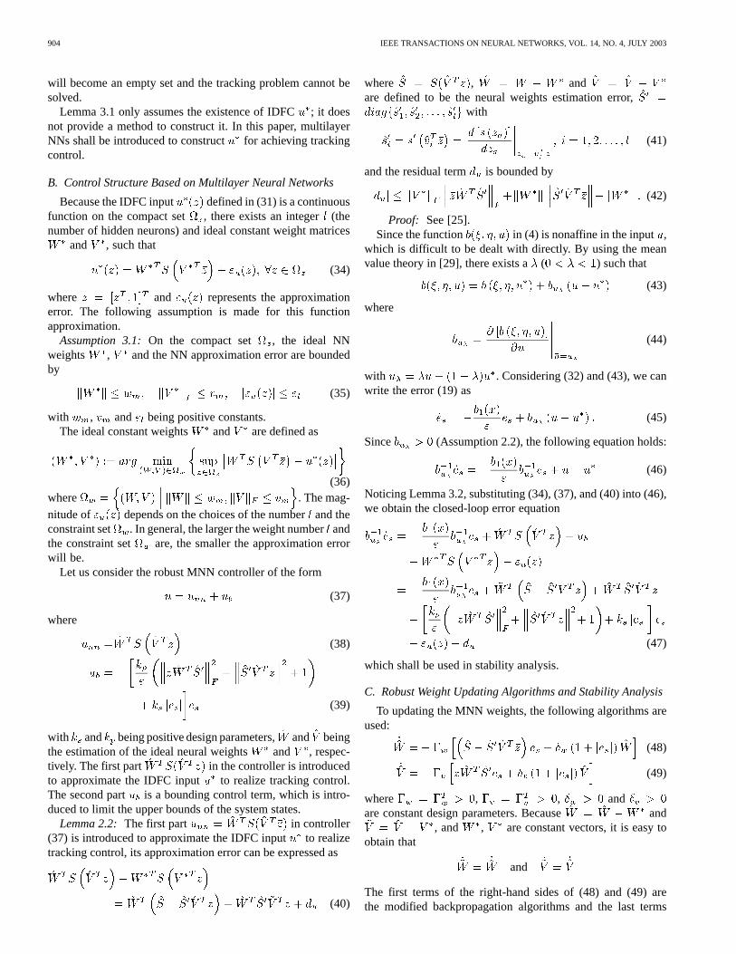
Fig. 1. Control system structure.

of them correspond to a combination of-modification [30]and -modification [31], which are introduced to improve therobustness in the presence of the NN approximation error. Itshould be noted that, (48) and (49) are special classes of severaladaptive laws proposed in [25]. The above learning algorithmshave a nice property as stated below.

Lemma 3.3:The updated learning algorithms (48) and (49)guarantee that , for bounded initial weights

and .Proof: Choose the Lyapunov function candidate

. Using theproperty , the time derivative of

along (48) and (49) is

Since , we have

Because every element of is not larger than one, we knowthat with being the NN hidden-layer node number.Therefore, once or .Because, and are positive constants, we conclude that

, . Q.E.D.The state feedback control structure is shown in Fig. 1. If the

high-gain observer in the dashed box is switched in, we have theoutput feedback control as will be discussed in Section IV.

Theorem 3.1:For system (1) with Assumptions 2.1–2.5 and3.1 being satisfied, let the controller be given by (37) and the NNweights be updated by (48) and (49). Then, there exist compactsets and , and positive constants, , , , , and

such that if

1) all initial states , ;2) , , , , , and

, then the trajectory of the system remainsin the compact set and the tracking error converges toa neighborhood of the origin which depends on (, ,

, , ).

Proof: The proof contains two steps. First, we assume thatholds for all time so that the transformation from

system (1) to the normal form (4) and the NN approximation inAssumption 3.1 are valid. With this assumption, we can provethat the tracking error converges to a small neighborhood of theorigin. Later, we will show that for a proper reference signal

and suitably chosen design parameters, do remainin the compact set if the system starts from a bounded initialset.

Step 1:Consider the Lyapunov function candidate

(50)

Differentiating (50) along (47)–(49), we have


Noticing Assumption 2.3, we obtain

Considering (42), Lemma 3.2 and the following inequalities:

(51)

(52)

we obtain

(53)

Further, noticing the following inequalities:

we have

(54)

where

(55)

(56)

Considering , inequality (54) canbe further written as

(57)

where constant

(58)

Now define

(59)

(60)

(61)

Since , , , , and , are positive constants, we knowthat , and are compact sets. Equation (57) showsthat once the errors are outside the compact setin (61). According to the standard Lyapunov theorem [32], weconclude that , , and are bounded. From (57) and (59),it can be seen that is strictly negative as long as is outsidethe compact set . Therefore, there exists a constantsuchthat for , the filtered tracking error converges to ,that is to say, with .Using Lemma 2.3, the internal dynamicwill converge to

(62)

Because converges to , is bounded as well.Consequently, is bounded.

Noting (9) and with constants and. Since , , from (12), we know that

(63)

Since is bounded, we know thatdecays exponentially. Inequality (63)

implies that the tracking error will converge to aneighborhood of the origin which depends on ( ).

In summary, under the assumption of , there ex-ists a constant such that 1) for all , the trackingerror converges to a neighborhood of the origin whichdepends on ( ); 2) the internal dynamics con-verges to for all ; and 3) the parameter estimate errors

and are bounded by if .Step 2:To complete the proof, we need to show that for a

proper choice of the tracking signal and control parame-ters, the trajectory do remain in the compact set . From

and , we can see that .Therefore


It follows from (63) and the fact that will converge to, we know that ,

, with , and. Hence

(64)

We now provide the conditions which guarantees ,. Define the compact set

(65)

the positive constant

(66)

the positive constants shown in (67)–(71) at the bottom of thepage. In summary, for all initial state , the desiredsignal , if control parameters , , , and

are chosen such that , , ,and , then the system statewill stay in for all

time. Furthermore, because the NN weights have been provenbounded for any bounded and (see Lemma 3.3), we

conclude that all signals of the closed-loop system are bounded.This completes the proof. Q.E.D.

Remark 3.3:Compared with the existing exact linearizationtechniques and NN control methods, the proposed robust adap-tive NN controller clearly has some intrinsic advantages. Forexample, there is no need to search for an explicit controllerto cancel the nonlinearities of the system exactly. In fact, eventhough the functions and in system (1) are known,it is in general not possible to get an explicit controller for feed-back linearization. In addition, the requirements of an off-linetraining phase and the persistent excitation condition are notneeded any more.

Remark 3.4: It is shown in (55) and (56) that smaller andmight be obtained by choosing a smaller and , which

may lead to a smaller tracking error. Nevertheless, from (60) itcan be seen that smaller and may cause larger NN weighterrors. In this case the control signal,, may be increased andout of region in which Assumptions 2.1, 2.2, and 2.5 hold. Onthe other hand, if and are chosen to be very large, so are

and , which will lead to a large tracking error will happen.Hence, the parameter and should be adjusted carefully inpractical implementations.

IV. OUTPUT FEEDBACK CONTROL

In Section III, the system states and the time derivatives ofthe outputs are supposed to be available for feed-back. This limits the application of the approach, because, inmany practical systems, only outputis measurable. In thissection, adaptive NN output feedback control is investigated for

(67)

(68)

(69)

(70)

and

(71)


nonaffine nonlinear systems with internal dynamics by using ahigh-gain observer to reconstruct the system states.

A. High-Gain Observer

Since only the output is measurable and the rest ofthe output derivatives are not available, we need to estimate

to implement the output feedback control. In thefollowing lemma, the high-gain observer used in [27] is pre-sented, which will be used to estimate the output derivatives ofsystem (4).

Lemma 4.1:Suppose the system output and its firstderivatives are bounded, so that with positive con-stants . Consider the following linear system:

(72)where is any small positive constant and the parametersto are chosen such that the polynomial

is Hurwitz. Then, we have the following.

1)

where withdenoting the th derivative of .

2) There exist positive constants and which only de-pending on , and , such that forall we have , .

Proof: The proof can be found in [27]. For completeness,it is given below.

1) From the last equation in (72), we have

Using (72) and the above equation yields

Differentiating it and utilizing (72), Item 1) follows.2) The derivatives of the vector

may be computed as follows:

(73)

where is the matrix corresponding to the homo-geneous part of (72) and independent of, and

. Since belongs to the com-pact set , and is bounded, there exist constants

such that . Then, for any , we

may find a constant such that for all thefirst term

in (73) is bounded by for each . Further,since , there exist constants , whichis independent of , such that the second term

in (73) is bounded byfor each . Fixing an arbitrarily small , then for, we have where

with the norm of the vector .As , , , and are independent of, the proof iscompleted. Q.E.D

B. Adaptive Neural Control by Output Feedback

Having the observer (72), we define

where

Lemma 4.1 shows that are bounded by the constants, hence , and are all bounded. Let and be the

estimates of and , respectively. The following lemmapresents the property of MNN’s when the input vectorisreplaced by the estimation.

Lemma 4.2:The NN estimation error can be expressed as

(74)

where , , ,with

, , and the residual termis bounded by

(75)

Proof: The proof can be obtained by following the similarprocedure in Lemma 3.2. It is omitted here.


C. Controller Structure and Stability Analysis

The output feedback controller is designed as follows:

(76)

where

(77)

(78)

with , , being the constant design parameters. Theabove controller contains three parts for different purposes. Thefirst part is introduced to approximate the IDFC inputfor achieving adaptive tracking control. The second partisa priori control term based on a nominal model or past controlexperience to improve the control performance. If no knowledgefor the plants is available, can be simply set to zero. Thethird part is a bounding control term, which is applied forlimiting the upper bounds of the system states such that the NNapproximation (34) holds on the compact set.

The MNN weight updating laws are taken as

(79)

(80)

where , , andare constant design parameters. The above learning algorithmshave a nice property as stated below.

Lemma 4.3:The updated learning algorithms (79) and (80)guarantee that , for bounded initial weights

and .Proof: The proof can be obtained by following the similar

procedure in Lemma 3.3. It is omitted here.Considering (43)–(46), the error system can be written as

(81)

Applying (34), (74), and (76), we obtain

(82)

Based on (82), closed-loop stability results are summarizedin Theorem 4.1.

Theorem 4.1:For system (4) with Assumptions 2.1, 2.2, 2.3,2.4 and 2.5 being satisfied, high-gain observer (72), controller(76) and adaptive laws (79) and (80), there exist a compact set

, and positive constants, , , , , and ,such that for any bounded and , if

1) the initial state ;2) the observer (72) is turned on at timein advance;3) , and ;

then all the signals in the closed-loop system are bounded,the system state , and the tracking errorconverges to a neighborhood of the origin which depends on( , ).

Proof: The proof contains two steps. We first assume thatholds for all time, which ensures that NN approx-

imation (34), Assumptions 2.1, 2.2, and 2.3 are valid. In thiscase, we prove the tracking error converging to an ()-neigh-borhood of the origin. Later, for a proper choice of the referencesignal and controller parameters, we show that () do re-main in the compact set for all time if the system starts froma bounded initial set.

Step 1:Consider the Lyapunov function candidate

(83)

Differentiating (83) along (82), we have

Noting , , (79),(80), we obtain

(84)

Since and (Assumption 2.3),we know that . Using

and , we have

Considering , , (75) and (78), andthe following inequalities:

we obtain (85), shown at the bottom of the next page. Since


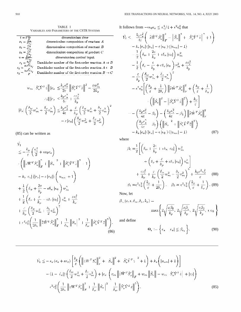
TABLE IVARIABLES AND PARAMETERS OF THECSTR SYSTEMS

(85) can be written as

(86)

It follows from that

(87)

where

(88)

(89)

Now, let

and define

(90)

(85)


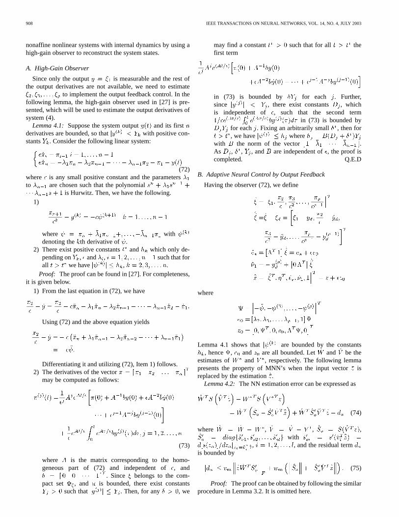
Fig. 2. � follows � (“- -”) (state feedback).

Since , , , , , , , and are positive constants andand are bounded, it follows that is also bounded, which

means that is a compact set. From (87)–(90), it is shownthat is strictly negative as long as is outside the set .Therefore, the filtered error is bounded, and there exists aconstant such that for , the filtered trackingerror converges to which is a neighborhood of the originthat depends on ( ).

The mapping of can be expressed in state spaceeqn (9). The solution for can be written as

. It follows that

(91)

Because , , from (12), we have

(92)

Since is bounded, we know that

decays exponentially. Inequality (92)

implies that the tracking error will converge to aneighborhood of the origin which depends on ( ).

Step 2:To complete the proof, we need to show that for aproper choice of the tracking signal and control parame-ters, the trajectory do remain in the compact set . Consid-ering a positive function and controller (76), the timederivative of along (81) is

(93)

Using (34), (76)–(78), we have

(94)

Since every element of is not larger than one, we knowthat

(95)

Therefore


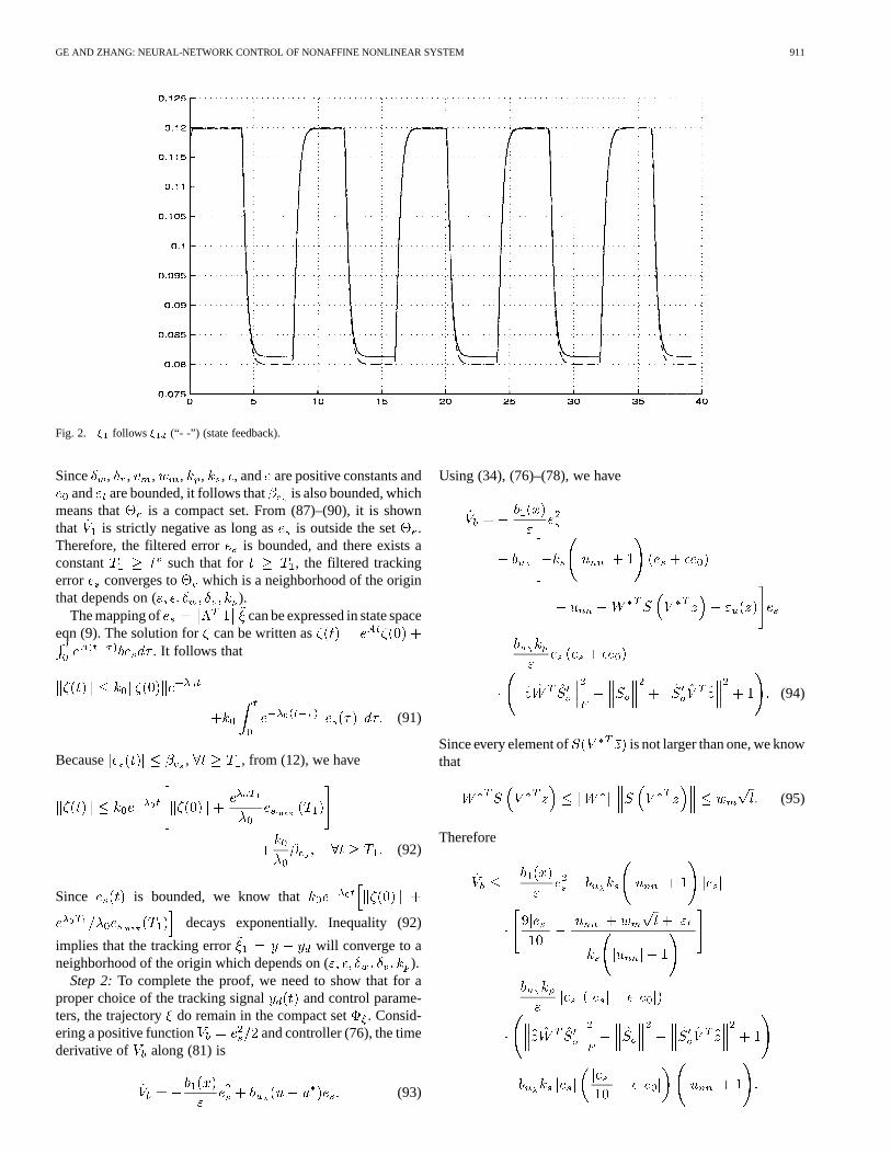
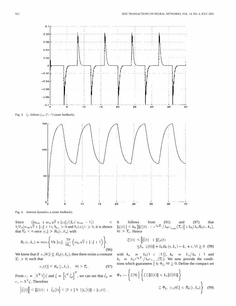
Fig. 3. � follows � (“- -”) (state feedback).

Fig. 4. Internal dynamics� (state feedback).

Since, and , it is shown

that once with

(96)We know that if , then there exists a constant

, such that

(97)

From and , we can see that

. Therefore

It follows from (91) and (97) that,

. Hence

(98)

with , and. We now provide the condi-

tions which guarantees , . Define the compact set

(99)


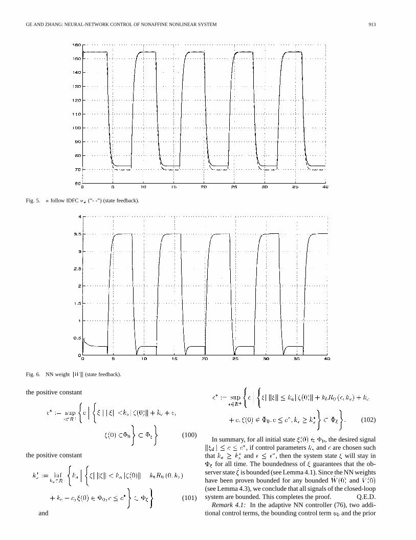
Fig. 5. u follow IDFC u (”- -”) (state feedback).

Fig. 6. NN weightk ^Wk (state feedback).


(100)


(101)

and

(102)

In summary, for all initial state , the desired signal, if control parameters and are chosen such

that and , then the system statewill stay infor all time. The boundedness ofguarantees that the ob-

server state is bounded (see Lemma 4.1). Since the NN weightshave been proven bounded for any bounded and(see Lemma 4.3), we conclude that all signals of the closed-loopsystem are bounded. This completes the proof. Q.E.D.

Remark 4.1: In the adaptive NN controller (76), two addi-tional control terms, the bounding control termand the prior


Fig. 7. NN weightk^V k (state feedback).

Fig. 8. � follows � (“- -”) (output feedback).

control term , are provided. The first one can be viewed as asupervisory control, which is introduced for limiting the upperbounds of the system variables such that holds. Thesecond one provides a chance that control engineers can useconventional techniques to design an initial controller and thenadd the adaptive NNs to work in parallel to achieve high trackingaccuracy. From (36), it can be seen that the closerandis, the smaller the ideal weight and will be. Consid-ering (88)–(90), one can see that smaller and will leadto smaller output tracking error. Therefore, if is designed ad-equately, the control performance can be improved. On the otherhand, even though is inadequate, the use of the above adap-tive NN controller still results in a stable tracking.

Remark 4.2: In Theorem 4.1, it requires that the observer(72) to be turned on at time in advance. This is because thehigh-gain observer may exhibit a peaking phenomenon and the

estimated state errors might be very large in the initial transientperiod. If the observer is turned on at timebefore the con-troller is put into operation, Lemma 4.1 guarantees that the stateestimation is bounded by the constant whichonly depends on , and and, therefore, the peaking ofthe controller can be avoided. Another method to overcome thepeaking problem is to introduce an estimate saturation or con-trol input saturation [33]–[35]. Thus, during the short transientperiod when the state estimates exhibit peaking, the saturationprevents the peaking from being transmitted to the plant.

V. SIMULATION STUDY

In this section, a practical isothermal continuous stirred tankreactor is simulated to illustrate the proposed state feedback andoutput feedback controllers.


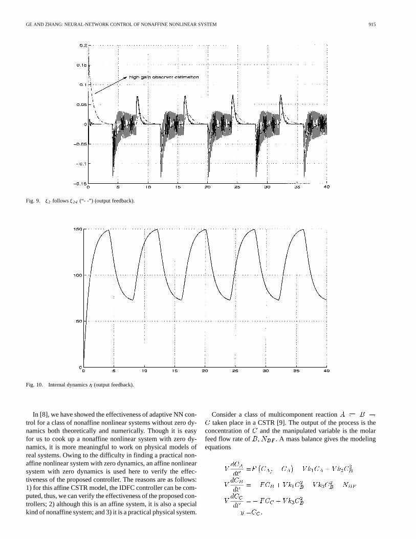
Fig. 9. � follows � (“- -”) (output feedback).

Fig. 10. Internal dynamics� (output feedback).

In [8], we have showed the effectiveness of adaptive NN con-trol for a class of nonaffine nonlinear systems without zero dy-namics both theoretically and numerically. Though it is easyfor us to cook up a nonaffine nonlinear system with zero dy-namics, it is more meaningful to work on physical models ofreal systems. Owing to the difficulty in finding a practical non-affine nonlinear system with zero dynamics, an affine nonlinearsystem with zero dynamics is used here to verify the effec-tiveness of the proposed controller. The reasons are as follows:1) for this affine CSTR model, the IDFC controller can be com-puted, thus, we can verify the effectiveness of the proposed con-trollers; 2) although this is an affine system, it is also a specialkind of nonaffine system; and 3) it is a practical physical system.

Consider a class of multicomponent reactiontaken place in a CSTR [9]. The output of the process is the

concentration of and the manipulated variable is the molarfeed flow rate of , . A mass balance gives the modelingequations


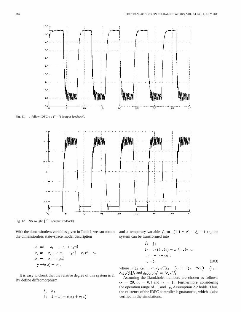
Fig. 11. u follow IDFC u (”- -”) (output feedback).

Fig. 12. NN weightk ^Wk (output feedback).

With the dimensionless variables given in Table I, we can obtainthe dimensionless state–space model description

It is easy to check that the relative degree of this system is 2.By define diffeomorphism

and a temporary variable thesystem can be transformed into

(103)

whereand .

Assuming the Damkholer numbers are chosen as follows:, and . Furthermore, considering

the operation range of and , Assumption 2.2 holds. Thus,the existence of the IDFC controller is guaranteed, which is alsoverified in the simulations.


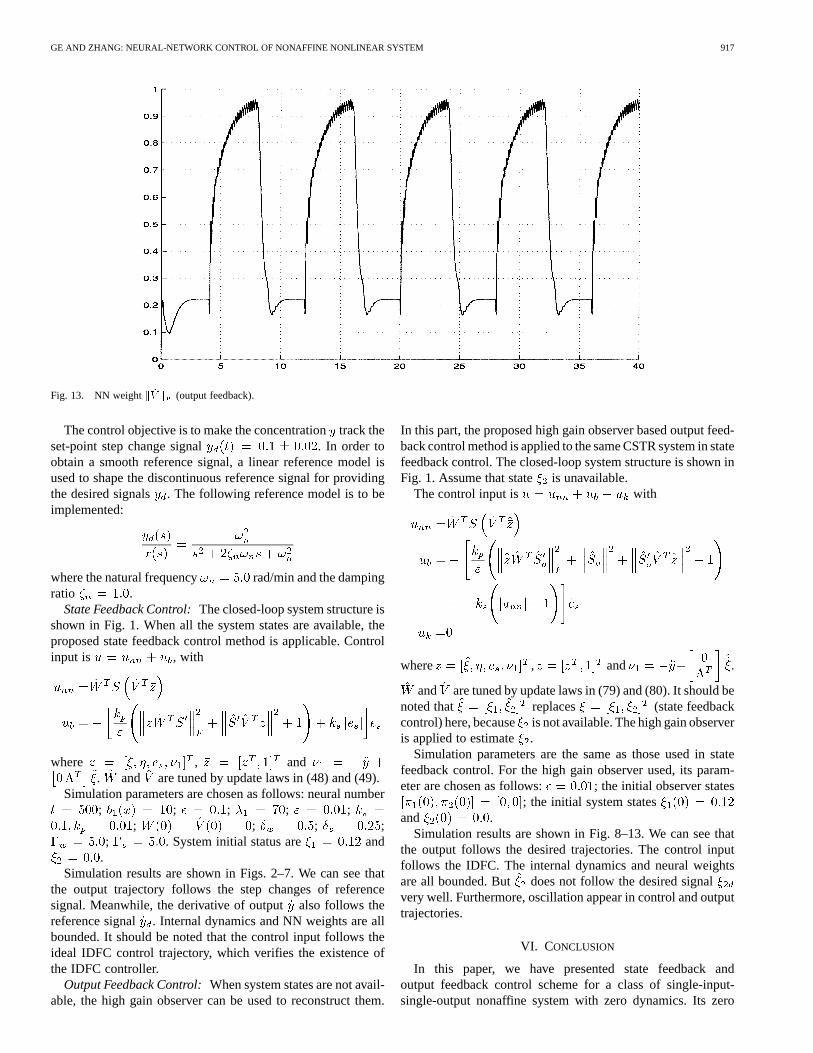
Fig. 13. NN weightk^V k (output feedback).

The control objective is to make the concentrationtrack theset-point step change signal . In order toobtain a smooth reference signal, a linear reference model isused to shape the discontinuous reference signal for providingthe desired signals . The following reference model is to beimplemented:

where the natural frequency rad/min and the dampingratio .

State Feedback Control:The closed-loop system structure isshown in Fig. 1. When all the system states are available, theproposed state feedback control method is applicable. Controlinput is , with

where , and. and are tuned by update laws in (48) and (49).

Simulation parameters are chosen as follows: neural number; ; ; ; ;

; ; ; ;; . System initial status are and

.Simulation results are shown in Figs. 2–7. We can see that

the output trajectory follows the step changes of referencesignal. Meanwhile, the derivative of outputalso follows thereference signal . Internal dynamics and NN weights are allbounded. It should be noted that the control input follows theideal IDFC control trajectory, which verifies the existence ofthe IDFC controller.

Output Feedback Control:When system states are not avail-able, the high gain observer can be used to reconstruct them.

In this part, the proposed high gain observer based output feed-back control method is applied to the same CSTR system in statefeedback control. The closed-loop system structure is shown inFig. 1. Assume that state is unavailable.

The control input is with

where , and .

and are tuned by update laws in (79) and (80). It should benoted that replaces (state feedbackcontrol) here, because is not available. The high gain observeris applied to estimate .

Simulation parameters are the same as those used in statefeedback control. For the high gain observer used, its param-eter are chosen as follows: ; the initial observer states

; the initial system statesand .

Simulation results are shown in Fig. 8–13. We can see thatthe output follows the desired trajectories. The control inputfollows the IDFC. The internal dynamics and neural weightsare all bounded. But does not follow the desired signalvery well. Furthermore, oscillation appear in control and outputtrajectories.

VI. CONCLUSION

In this paper, we have presented state feedback andoutput feedback control scheme for a class of single-input-single-output nonaffine system with zero dynamics. Its zero


dynamics are assumed to be exponentially stable. Based onimplicit function theory, stable adaptive NN controllers aredeveloped for both state and output feedback control. Theproposed design guarantees the stability of the closed-loopadaptive system and the convergence of the tracking errors.

REFERENCES

[1] A. Isidori, Nonlinear Control System, 2nd ed. Berlin, Germany:Springer-Verlag, 1989, 1995.

[2] M. Krstic, I. Kanellakopoulos, and P. V. Kokotovic,Nonlinear and Adap-tive Control Design. New York: Wiley, 1995.

[3] F. L. Lewis, S. Jagannathan, and A. Yesildirek,Neural Network Controlof Robot Manipulators and Nonlinear Systems. London, U.K.: Taylorand Francis, 1999.

[4] S. S. Ge, T. H. Lee, and C. J. Harris,Adaptive Neural Network Controlof Robotic Manipulators. London, U.K.: World Scientific, 1998.

[5] L. X. Wang, Adaptive Fuzzy Systems and Control: Design and Anal-ysis. Englewood Cliffs, NJ: Prentice-Hall, 1994.

[6] R. Marino and P. Tomei,Nonlinear Adaptive Design : Geometric, Adap-tive, and Robust. London, U.K.: Prentice-Hall, 1995.

[7] A. R. Teel, R. R. Kadiyala, P. V. Kokotovic, and S. S. Sastry, “Indirecttechniques for adaptive input-output linearization of nonlinear systems,”Int. J. Contr., vol. 53, pp. 193–222, 1991.

[8] S. S. Ge, C. C. Hang, and T. Zhang, “Nonlinear adaptive control usingneural network and its application to cstr systems,”J. Process Contr.,vol. 9, pp. 313–323, 1998.

[9] J. P. Calvet, “A Differential Geometric Approach for the Nominal andRobust Control of Nonlinear Chemical Process,” Ph.D. dissertation,School Chem. Eng., Georgia Inst. Technol., Atlanta, GA, 1989.

[10] G. R. Slemon and A. Straughen,Electric Machines. Reading, MA: Ad-dison-Wesley, 1980.

[11] H. K. Khalil, Nonlinear Systems. Upper Saddle River, NJ: Prentice-Hall, 1996.

[12] J. J. Romano, “I-o map inversion, zero dynamics and flight control,”IEEE Trans. Aerospace Electron. Syst., vol. 26, pp. 1022–1029, Nov.1990.

[13] J. E. Slotine and W. Li,Applied Nonlinear Control. Englewood Cliffs,NJ: Prentice-Hall, 1991.

[14] A. Isidori, S. S. Sastry, P. V. Kototovic, and C. I. Byrnes, “Singularlyperturbed zero dynamics of nonlinear systems,”IEEE Trans. Automat.Contr., pp. 1625–1631, Oct. 1992.

[15] C. J. Tomlin and S. S. Sastry, “Bounded tracking for nonminimum phasenonlinear systems with fast zero dynamics,” inProc. 35th IEEE Conf.Decision Control, vol. 2, 1996, pp. 2058–2063.

[16] H. Schwarz, “Changing the unstable zero dynamics of nonlinear systemsvia parallel compensation,” inUKACC Int. Conf. Control, vol. 2, Sept.2–5, 1996, pp. 1226–1231.

[17] J. Huang, “Output regulation of nonlinear systems with nonhyperboliczero dynamics,”IEEE Trans. Automat. Contr., vol. 40, pp. 1497–1500,Aug. 1995.

[18] W. Yim, “End-point trajectory control, stabilization, and zero dynamicsof a three-link flexible manipulator,” inIEEE Int. Conf. Robotics Au-tomation, vol. 2, 1993, pp. 468–473.

[19] K. S. Narendra and K. Parthasarathy, “Identification and control of dy-namic systems using neural networks,”IEEE Trans. Neural Networks,vol. 1, pp. 4–27, Mar. 1990.

[20] A. U. Levin and K. S. Narendra, “Control of nonlinear dynamical sys-tems using neural networks-Part II: Observability, identification, andcontrol,” IEEE Trans. Neural Networks, vol. 7, pp. 30–42, Jan. 1996.

[21] A. Yesidirek and F. L. Lewis, “Feedback linearization using neural net-works,” Automatica, vol. 31, no. 11, pp. 1659–1664, 1995.

[22] M. M. Polycarpou, “Stable adaptive neural control scheme for nonlinearsystems,”IEEE Trans. Automat. Contr., vol. 41, pp. 447–451, Mar. 1996.

[23] C. J. Goh, “Model reference control of nonlinear systems via implicitfunction emulation,”Int. J. Contr., vol. 60, pp. 91–115, 1994.

[24] S. S. Ge, C. C. Hang, and T. Zhang, “Adaptive neural network controlof nonlinear systems by state and output feedback,”IEEE Trans. Syst.,Man, Cybern. B, vol. 29, pp. 818–828, Dec. 1999.

[25] S. S. Ge, C. C. Hang, T. H. Lee, and T. Zhang,Stable Adaptive NeuralNetwork Control. Boston, MA: Kluwer, 2001.

[26] J. Tsinias and N. Kalouptsidis, “Invertability of nonlinear analyticsingle-input systems,”IEEE Trans. Automat. Control, vol. AC-28, pp.931–933, Mar. 1983.

[27] S. Behtash, “Robust output tracking for nonlinear system,”Int. J. Contr.,vol. 51, no. 6, pp. 1381–1407, 1990.

[28] W. Hahn, Stability of Motion. Berlin, Germany: Springer-Verlag,1967.

[29] T. M. Apostol, Mathematical Analysis. Reading, MA: Ad-dison-Wesley, 1957.

[30] P. A. Ioannou and J. Sun,Robust Adaptive Control. Englewood Cliffs,NJ: Prentice-Hall, 1995.

[31] K. S. Narendra and A. M. Annaswamy, “A new adaptive law for robustadaptation without persistent excitation,”IEEE Trans. Automat. Control,vol. AC-32, pp. 134–145, Feb. 1987.

[32] K. S. Narendra, Y. H. Lin, and L. S. Valavani, “Stable adaptive con-troller design-Part II: Proof of stability,”IEEE Trans. Automat. Contr.,vol. AC-25, pp. 440–448, Mar. 1980.

[33] H. K. Khalil, “Adaptive output feedback control of nonlinear systemrepresented by input-output models,”IEEE Trans. Automatic Contr., vol.41, pp. 177–188, Feb. 1996.

[34] B. Aloliwi and H. K. Khalil, “Robust adaptive output feedback controlof nonlinear systems without persistence of excitation,”Automatica, vol.33, no. 11, pp. 2025–2032, 1997.

[35] M. Jankovic, “Adaptive output feedback control of nonlinear feedbacklinearizable system,”Int. J. Contr., vol. 10, pp. 1–18, 1996.

Shuzhi Sam Ge(S’90–M’92–SM’00) received theB.Sc. degree from Beijing University of Aeronauticsand Astronautics (BUAA), Beijing, China, in 1986,and the Ph.D. degree and the Diploma of ImperialCollege (DIC) from Imperial College of Science,Technology, and Medicine, University of London,London, U.K., in 1993.

From 1992 to 1993, he did his postdoctoralresearch at Leicester University, Leicester, U.K.Since 1993, he has been with the Department ofElectrical and Computer Engineering, the National

University of Singapore, Singapore, where he is currently as an AssociateProfessor. He has authored and co-authored more than 100 international journaland conference papers, two monographs, and co-invented two patents. Hiscurrent research interests are nonlinear control, neural networks and fuzzylogic, robotics and real-time implementation.

Dr. Ge has served as an Associate Editor, IEEE TRANSACTIONS ONCONTROL

SYSTEMS TECHNOLOGY since 1999, and has been a Member of the TechnicalCommittee on Intelligent Control of the IEEE Control System Society since2000. He was the recipient of the 1999 National Technology Award, the 2001University Young Research Award, and the 2002 Temasek Young InvestigatorAward, Singapore. He serves as a Technical Consultant to local industry.

Jin Zhang was born in Xi’an, Shaanxi Province,P.R. China, in 1974. He received the B.Eng. degreefrom the Department of Automatic Control, BeijingUniversity of Aeronautics and Astronautics (BUAA),P.R. China, in 1997. He is currently pursuing thePh.D. degree with the Department of Electrical andComputer Engineering, the National University ofSingapore, Singapore.

His research interests include adaptive non-linear control, neural-network control, and controlapplications.

neural-network control of nonaffine nonlinear system with zero

Documents