network performance analysis based on histogram workload
TRANSCRIPT

Network Performance Analysis based on HistogramWorkload Models (Extended Version)
Enrique Hernandez-Orallo Joan Vila-CarboDepartamento de Informatica de Sistemas y Computadores
Universidad Politecnica de Valencia Camino de Vera SN Valencia Spain
ehernandezdiscaupves jviladiscaupves
January 23 2008
Abstract
Network performance analysis relies mainly on two models a workloadmodel and a performance model This paper proposes to use histogramsfor characterising the arrival workloads and a performance model based ona stochastic process This new stochastic process works directly with his-tograms using a set of specific operators The result is the buffer occupancydistribution The loss rate and network delay distribution can be obtainedusing this distribution Three traffic models are proposed the first model (theHD model) is a basic histogram model that is compact and reflects only firstorder statistics The other two captures second order statistics the (HD(N)
model) is based on obtaining several histograms using different time scales andthe (the HD(H) model) is based on the Hurst parameter and it is long-rangedependent
This method is evaluated using several real traffic network workloads andthe results show that the model is very accurate The model forms an excellentbasis for a decision support tool to allow system architects to predict thebehavior of computer networks
KEYWORDS Network Performance Analysis Traffic ModellingStochastic Analysis
1 Introduction
Network performance relies mainly on routersrsquo queues (buffers) Therefore queue-ing analysis plays a crucial role in their design and performance In the simplestqueueing analysis a traffic is fed into a single-server queue of limited capacity witha given service rate and we wish to determine information about the queue utiliza-tion Systems performance analysis relies mainly on two models a workload modeland a performance model The workload model capture the resource demands and
1
workload intensity characteristics This model must capture the static and dynamicbehavior of the real load and it must be compact and accurate The performancemodel is used to predict the performance of a system as a function of the systemdescription and the workload model
Understanding the nature of the traffic is critical to properly model a computernetwork system There has been a considerable amount of work on traffic charac-terisation in the literature [1] In classic networks the Poisson process has sincelong been used for call arrivals because calls are generated independently fromeach other However Internet traffic does not fit into this description Two pio-neering articles [2] [3] showed two properties i) self-similarity counts of packetarrivals in equally-spaced intervals of time are long-range time dependent and havea large coefficient of deviation and ii) heavy tailed packet inter-arrival have amarginal distribution that has a longer tail than the exponential Recently studieshas shown that this arrival process tends toward Poisson as load increases [4] [5]Several distributions were proposed to fit these traffic characteristics The Paretoand Weibull distributions are often used in order to reflect the heavy-tailed distri-bution The self-similarity property can be modeled by an aggregate of multipleheavy-tailed ONOFF sources More complex models are based on fractional Gaus-sian noise (fGN) fractional autoregressive integrate moving average (fARIMA) andwavelets [6]
Several queueing analysis methods have been proposed to model and obtainperformance parameters [7] Markov Modulated Poisson Process (MMPP) [8 9]Switched Batch Bernouilli Process (SBBP) [10] or Discrete Gaussian Models [1]There are several practical problems with these models First we must fit the trafficwith the model Nevertheless the problem is that when the number of parametersare high the model usually become intractable so we must use few parameters andthis implies losing precision Second most of the papers deal with the tail probability(or overflow probability) P (Q gt t) rather than the loss probability Neverthelessreal networks have finite buffer so it is necessary to study the loss probability infinite buffer systems (PL(x)) In infinite queue models the loss probability is oftenapproximated as PL(x) asymp P (Q gt x) However this approximation usually providesan upper bound (sometimes a very poor bound) to the loss probability [11] For thisreason the authors of [11] presented an estimation for the loss probability based onthe tail probability Therefore for network performance evaluation is better to usea model with finite buffer
Several papers have proposed the use of histograms as the basis for performancemodels The Histogram Model [1213] was introduced by Skelly to predict buffer oc-cupancy and loss rate for multiplexed streams These works use an analysis methodbased on a MD1N queueing system The number of ATM cells generated dur-ing a frame period is approximated to a Poisson distribution with a given rate λFor a given video sequence λ is modelled as a histogram The buffer occupancy iscalculated by solving the MD1N system as a function of λ and then weightingthe solutions according to the histogram probabilities These methods yields goodresults with a reduced number of cells in the buffer but the inaccuracy increases
2
with the number of cells Another histogram-based performance analysis was pre-sented in [14] The method is based on a modification of the MVA (Mean ValueAnalysis) algorithm for resolving Queueing Network Models (QNM) The drawbackof these models is that they resolve for each value of the histograms classes indepen-dently (using MD1N or MVA) not taking into account the dependencies betweenthe histogram classes A more complex approach is the distrete time SBBPG1queue [10] The SBBP process is characterized by a probability generating function(pgf) and two states The system is resolved only for the infinite capacity queuecase This model has two drawbacks when it is applied to real-traffic modeling thecomplexity of definining the pgf from the traffic (the number of states can be verylarge) and that there is no solution for limited capacity buffer
The criteria for a practical performance model can be resumed in three points[15]
1 the traffic model is defined by a small number of parameters and reflects firstand second order statistics
2 the model will accurately predict the performace parameters
3 it is easy and amenable to analysis
In this paper we propose using histograms as the network traffic model and in-troduce a stochastic process that works directly with histograms This stochasticprocess obtains the queue length distribution as a histogram using a finite queuemodel The proposed method does not require approximating traffic to a Poissondistribution nor solving queueing models Our model assumes that the traffic isstationary and the inter-arrival time distribution in a period is constant (determin-istic) This basic histogram model will be refered to as the HD model (HistogramDeterministic inter-arrival distribution) Based on this basic model we introducetwo new models ii) the HD(N) model is based on obtaining several histograms usingdifferent time scales and iii) the HD(H) model is based on the Hurst parameter andit is long-range dependent The best way to verify the correctness of our modelis to compare the predicted results to the ones obtained using a real model withreal traffic These experiments are detailed in section IV and the results are veryaccurate These evaluations also analyse the influence of the number of histogramclasses on precision showing that 10 classes are enough to obtain good results
2 Traffic Workload Models
In this section we present three workload models based on histograms The first oneis a simple workload definition that only capture first order statistics The other twoare extensions of the first one in order to capture second order statistics (long-rangedependence)
3
0 10000 20000 30000 40000 50000 60000 70000 80000 900000
1 Mb
2 Mb
3 Mb
4 Mb
5 Mb
6 Mb
7 Mb
8 Mb
frame number
load
in p
erio
d (b
its)
(a)
0 1 2 3 4 5 6 7 80
01
02
03
04
05
06
07
08
09
1
load in period in Mbs
prob
abili
ty
(b)
Figure 1 Traffic trace used as illustration It corresponds to a 1-hour IP traffic trace (a) Numberof bits per period (40ms) (b) Arrival load histogram using 10 classes
21 Basic Histogram Workload Model
Network workloads will be characterized by the number of transmission units pro-duced by a traffic source during a pre-established time period called the sam-pling period1 Concretely let At be a discrete random variable representing theamount of traffic entering a network link during the kth sampling interval ThenAt t = 1 2 (At for short) is a discrete stochastic process with a statespace I that is the set of integers between 0 and the maximum sample size Smax(I = 0 1 Smax)
A sample realization of this process at t = 1 2 (at for short) is shownin Figure 1a This traffic trace was extracted from the MAWI traffic traces [16]Specifically we took a 1-hour trace of IP traffic corresponding to Jan 09 20071200 through 1300 of a 150 Mbs trans-pacific line (samplepoint-F) This traffictrace has an average rate of 109 Mbs Using a sampling period of T = 40 ms (25samples per second) the resulting traffic trace has 90000 frames and a state spaceof I = 0 1 middot middot middot 8Mb
Working with this huge state space can be cumbersome So we are going toreduce this state space using n subintervals or bins Consequently if we have arange of [0 Smax] then the interval size will be lA = Smaxn Using these intervalswe define a binned process At2 that have a reduced state space I prime = 0 (nminus1) The correspondence between some value a in the traffic state space of I and itssubinterval or class number i (state space I prime) is given by the following equation
i = classA(a) =
lfloora
lA
rfloor(1)
1For convenience we use the bit as the base unit There is no variation in the precision of theresults using another unit (bytes packets)
2Note the calligraphic font style Along the paper the calligraphic font style (A) will denotethe binned random variable with the reduced state space and the normal font style (A) will denotethe original random variable
4
The inverse function is defined as the midpoint of the subinterval
a = midA(i) = lA middot i+ lA2 (2)
For our traffic model we assume that the process At (and consequently the binnedprocess At) is ergodic (and stationary) Being ergodic means that we can estimatethe process statistics from the observed values of a single realization or time seriesat Being stationary means that all the binned random variables At have the samemarginal distribution In other words the distribution does not change on time andwe can work with only one random variableA that has the same statistical propertiesof all the random variables At of the binned process Assuming that the processis stationary is a simplification necessary for our model It is a matter of fact thattraffic workload is not stationary in the same day the traffic load at 5 am canbe very different than the traffic load at 12 pm or the traffic in the weekend isvery different that the traffic in a working day This implies that the precision of themodel will depend on the time range of the traffic studied It is clear that short-termtraffic analysis will be more precise than long-term traffic analysis This topic willbe studied in the experiments section
Another assumption of our model regards to the packet inter-arrival time dis-tribution in a period (the time between the arrivals of successive packets) Thisdistribution can be approximated using several distributions as detailed in Table1 In this table we can see the probability mass function (pmf) of the distribu-tion and a sample of the temporal distribution The simplest distributions are thedeterministic (uniform) or burst mode Nevertheless this distribution is usuallymodeled using Poisson or Pareto distributions For example the MAWI traffic hasthe inter-arrival distribution of Figure 2a that clearly shows a heavy-tailed distri-bution Nevertheless if we zoom in this graph and show the distribution for lessthan 1ms (see Figure 2b) the result is that 75 of the interarrival time is less than005ms So the deterministic distribution can be used as a simple model of theinterarrival distribution
We assume that traffic arrives at uniform rate in a period but the number ofarrivals in a period have a distribution modelled by the binned random variableobtained from the traffic (that is A) In other words if we have N packets or bits ina sampling period T the inter-arrival distribution is deterministic with value NT
Using a traffic series we can obtain the set of interval probabilities pA(i) (thatis the pmf) This will be denoted as
p(A) = [pA(i) i = 0 nminus 1] (3)
Using the MAWI traffic trace with n = 10 we have the following pmf p(A) =[00003 00002 00021 00641 02663 03228 02345 00980 00110 00005] withan interval length (lA) of 08 Mb That is the probability of pA(0) = 00003 corre-sponds to the first interval [0 08[ Mb with midpoint 04 Mb The probability of thesecond interval [08 16[ Mb is pA(1) = 00002 and so on If we plot this pmf we havea kind of histogram of the original traffic trace (see Figure 1b) For convenience
5
Mode Inter-arrival distribution pmf temporal arrival
Deterministic pX(x) =
(1 x = T
N
0 x 6= TN
time
T
TN
0
1
0 1 2 3 4 5 6 7 8 9interarrival timeTN0
1
05
P(x)
0time
T
TN
0
1
0 1 2 3 4 5 6 7 8 9interarrival timeTN0
1
05
P(x)
0
Burst pX(x) =
8gtltgtNminus1
Nx = 0
0 0 lt x lt T1N
x = Ttime
T
0
0
1
0 1 2 3 4 5 6 7 8 9interarrival time0
1
05
P(x)
0time
T
0
0
1
0 1 2 3 4 5 6 7 8 9interarrival time0
1
05
P(x)
0
Poisson pX(x) = Poi(λ) λ = TN
0
100
0 1 2 3 Tn 5 6 7 8 9interarrival timeTN
1
05
P(x)
0time
T
=TN
0
100
0 1 2 3 Tn 5 6 7 8 9interarrival timeTN
1
05
P(x)
0time
T
=TN
Pareto pX(x) = kxm
k
xk+1 E[X] = TN
0
100
0 1 2 3 4 5 6 7 8 9interarrival timeTN
1
05
P(x)
0time
T
E[X]=TN
0
100
0 1 2 3 4 5 6 7 8 9interarrival timeTN
1
05
P(x)
0time
T
E[X]=TN
Table 1 Approximations to the inter-arrival distributions The last column shows an illustrativetemporal arrival sequence Our traffic model is based on a deterministic arrival distributionNevertheless the inter-arrival distribution is usually modeled using Poisson or Pareto distribution
the X-axis of the histogram will show the midpoint rather than the interval number(that is midA(i)) This way we can see the distribution for the original state space
Summing up the random variable A will usually be managed through just twoattributes the pmf (p(A)) and the interval length (lA) Abusing notation we willuse the term histogram for referring to the pmf of the random variable A
In short our traffic model is described using a histogram and a interval lengthThis model assumes that the traffic is stationary and the inter-arrival time distri-bution in a period is constant (deterministic) This basic histogram model will berefered to as the HD model (Histogram Deterministic inter-arrival distribution)
Some important operators on random variables that will be used throughout thepaper are introduced bellow
bull The mean value (or expectation) of X is defined as E[X ] =sumnminus1
0 pX (i)middoti Themaximum of X is defined as M [X ] = nminus 1 And the variance of X is definedas V ar(X ) =
sumnminus10 (i minus E[X ])2 middot pX (i) In the previous example M [A] = 9
E[A] = 506 and V ar(A) = 127 It is easy to obtain the mean and variationin the traffic state space using the interval size lX E[X] = lX middotE[X ]+lX2 andV ar(X) = (lX)2 middotV ar(X ) For example E[A] = 08times106 middot506 + 08times1062 =445Mb and V ar(A) = (08times 106)2 middot 127 = 814times 1011
bull The scalar multiplication of X by a constant c is a new binned variable Y = cmiddotXwhere lY = c middot lX and pY(i) = pX (i) for i = 0 nminus 1 That is multiplying bya scalar only affects the interval size
bull The sum of two independent binned random variables X and Y is defined usingthe convolution operator denoted as XotimesY The convolution is only defined forrandom variables with the same interval length Let n and m be the number
6
0 20 40 60 80 100 120 14010
minus8
10minus6
10minus4
10minus2
100
Interarrival time (ms)
prob
abili
ty (
log
scal
e)
(a)
0 02 04 06 08 10
01
02
03
04
05
06
07
08
09
1
Interarrival time (ms)
Pro
babi
lity
PMF (Histogram)CDF (Cumulative Dist)
(b)
Figure 2 MAWI inter-arrival distribution (a) Probability in log scale that clearly shows a heavy-tailed distribution (b) Zoom for inter-arrival time less than 1ms We represent the cumulativedistribution and the histogram We can see that more than 75 of the inter-arrival distribution isbelow 005ms
of intervals of X and Y respectively and let lX = lY be their interval lengthThe convolution X otimesY is a new variable Z with n+mminus 1 intervals the sameinterval length lZ = lX = lY and pZ(i) =
sumik=0 pX(iminus k) middot pY (k)
22 Second-order Statistics models
In this section we study how the histogram changes depending on the samplingperiod Based on these studies we propose two new traffic models that reflectssecond-order statistics
Let At be the stationary process described in the previous section with variance
σ2 and autocorrelation function r(k) = Cov(At At+k)σ2 We define A(m)
t as them-aggregated process of At that is obtained by aggregating and averaging thedata in Ak by blocks of size m
A(m)t =
1
m(Am(tminus1)+1 + middot middot middot+ Amt) (4)
and r(m)(k) is defined as the autocovariance function of A(m)t The first effect
of the aggregation of the process is to smooth the traffic rate in each period sothe variation is reduced How this variation changes depending on the factor ofaggregation is related to the study of the self-similarity of a process
A self-similar process has the property that when aggregated the new processhas the same autocorrelation function as the original That is the process At iscalled second-order self-similar with Hurst parameter H = 1minus β2 if
V ar(A(m)t ) = σ2mminusβ and r(m)(k) = r(k) forallm = 1 2 (5)
If 0 lt H lt 05 the process is short-range dependent (SRD) and if 05 lt H lt 1 theprocess is long-range dependent (LRD)
7
0 05Mb 1Mb 15Mb 2Mb 25Mb0
02
04
06
08
1
0 05Mb 1Mb 15Mb 2Mb 25Mb0
02
04
06
08
1
0 05Mb 1Mb 15Mb 2Mb 25Mb0
02
04
06
08
1
m=1T=001s m=4T=004s m=10T=01s
0 05Mb 1Mb 15Mb 2Mb 25Mb0
02
04
06
08
1
m=40T=04s
0 05Mb 1Mb 15Mb 2Mb 25Mb0
02
04
06
08
1
m=100T=1s
(a)0 05Mb 1Mb 15Mb 2Mb 25Mb0
02
04
06
08
1
0 05Mb 1Mb 15Mb 2Mb 25Mb0
02
04
06
08
1
0 05Mb 1Mb 15Mb 2Mb 25Mb0
02
04
06
08
1
m=1T=001s m=4T=004s m=10T=01s
0 05Mb 1Mb 15Mb 2Mb 25Mb0
02
04
06
08
1
m=40T=04s
0 05Mb 1Mb 15Mb 2Mb 25Mb0
02
04
06
08
1
m=100T=1s
0 05Mb 1Mb 15Mb 2Mb 25Mb0
02
04
06
08
1
0 05Mb 1Mb 15Mb 2Mb 25Mb0
02
04
06
08
1
0 05Mb 1Mb 15Mb 2Mb 25Mb0
02
04
06
08
1
0 05Mb 1Mb 15Mb 2Mb 25Mb0
02
04
06
08
1
0 05Mb 1Mb 15Mb 2Mb 25Mb0
02
04
06
08
1
(b)
Figure 3 (a) Histograms for aggregated processes A(1)t A(4)
t A(10)t A(40)
t and A(100)t We can see
that the distribution shrinks as m increases revealing the self-similarity property of the traffic (b)Histograms generated using the Hurst parameter in the HD(H)traffic model using as base periodT = 001s We can see that the histograms are very similar to the upper ones
Note that this means that the process is distributionally self-similar the pro-cesses At and A(m)
t have the same distribution up to a scaling factor Figure 3ashows the histograms for several m-agregated processes with m = 1 4 10 40 and100 using a base period of T = 001s We can see that the histograms shrinks asm increases This clearly denotes the self-similitary property of the MAWI trafficThe variance of the m-aggregated process can be obtained as
V ar(A(m)t ) = m2Hminus2 middot V ar(At) = m2Hminus2σ2 (6)
The graph of the variance log(V ar(A(m)t )) versus log(m) is called the variance-
time plot Using this graph we can obtain the Hurst parameter fitting a least-squareline with slope β = 2H minus 2 through the resulting points ignoring those for smallm In Figure 4 we can see the variance time plot of the MAWI traffic using a baseperiod of 1ms This traffic has a Hurst parameter of about 085 so it is long-rangedependent
For the binned process At we can obtain a similar expression for Equation 7Let σ2 = V ar(At) then
V ar(At) = (lA)2 middot V ar(At) = (lA)2 middot σ2 = σ2
We also define the binned processes A(m)t for A(m)
t We have that
V ar(A(m)t )) = (lA(m))2 middot V ar(A(m)
t ) = m2Hminus2σ2
Assuming lA(m) = lA we have
V ar(A(m)t ) =
m2Hminus2σ2
(lA)2=m2Hminus2(lA)2 middot σ2
(lA)2= m2Hminus2σ2 (7)
8
100
101
102
103
104
10minus4
10minus3
10minus2
10minus1
100
m (aggregation size) minus log scale
Var
ianc
e minus
log
scal
e
slope minus1Trace dataHD(H) fit
Figure 4 Variance time plot of the MAWI traffic (Base period for m=1 is 1ms) The line withslope β = minus1 determines if a traffic is SRD or LRD If the variance plot is above this line thetraffic is LRD otherwise is SRD Thus the MAWI traffic is LRD with Hurst parameter 085
In order to consider the second order statistics we propose two new models thatare based on the basic histogram model HD The first one is based on obtainingthe histogram for several time scales The HD model has only one histogram fora given sample period TA But if we have several histograms for several periodsthen the variance will be different on several time scales For example we can usedthe histograma of Figure 3a with sampling periods 001s 01s 1s 10s and 100sWe have 5 histograms with different variances Therefore this model can reflect thevariance of the traffic on diferent time scales Nevertheless this model of the trafficdoes not capture the self-similarity characteristics of the traffic
This model will be refered to as HD(N) where (N) reflects that there are differenthistograms for several sample periods (or aggregates) One of the problem of thismodel is the selection of the number and values of the sample periods If we usetwo much samples periods the model is too complex So we must select only 2or 3 sample periods in order to make the model compact For the selection of thesampling period we can use a set of fixed period (for example 001s 01s and 1s) oranother approach based on curve fitting
The second model is based on the Hurst parameter The idea is to estimate thehistograms of the m-aggregated processes A(m)
t using the histogram of the base
process At By Equation 7 we know that V ar(A(m)t ) = m2Hminus2σ2 and lA(m) = lA
As previously stated self-similarity means that processes At and A(m)t have
the same distribution up to a scaling factor In this case the scaling factor for thevariance is m2Hminus2 The proposed solution is to modify (to scale) the histogram Aaccording to this scaling factor The resulting histogram will have a distributionsimilar to the original but the variance will be m2Hminus2σ2 This process is rather
9
p(A)
p(Q)
b=4 (B = 35Mb)
r=5(R=100Mbs)
0
1
0 1 2 3 4 5 6 7 8 9
0
1
0 1 2 3 4
Figure 5 Sample scenario for the basic finite-buffer occupancy analysis The output rate isR=100 Mbs (that is a service rate of 4 Mb per sampling period) and a bounded buffer lengthof 35 Mb These values corresponds to classes r = 5 and b = 4 The process obtain the queuehistogram Q given the arrival histogram A
tricky and it is detailed in the Appendix A This appendix describes the function A =HScale(AmH) that calculates the histogram A and length size for an aggregationof m and a Hurst parameter H For example we can generate the histograms forthe MAWI traffic using a base period of T = 001s and the same aggregations thatin the HD(N) model The results are shown in Figure 3b and we can see that thehistograms are very similar to the real ones This model will be referred to as theHD(N) model and its defined with a histogram and the Hurst parameter
3 Network Peformance Model
This section introduces a stochastic process based on histograms for obtaining thebuffer occupancy distribution First we describe the model using the basic trafficmodel (HD) Next we present a simple extension of the basic model for the HD(N)
and HD(H) traffic models Finally using the buffer occupancy distribution we cancalculate several Quality of Service (QoS) parameters
31 Basic Finite-Buffer Occupancy Analysis
The analysis starts by considering a single node as shown in Figure 5 Input trafficis supplied through buffers of finite capacity These buffers accumulate pendingtraffic that cannot be transmitted over a sampling period The system will be saidto be stable if the pending traffic converges to a finite value The server discipline isFirst Come First Served (FCFS) with deterministic (constant) distribution UsingKendallrsquos notation we are trying to resolve a HDD1K queue
The queue or buffer length can be expressed using a recurrence equation assuming
10
a discrete time space T = 0 1 2 Let Q[k] be the queue length for period k isin T 3
Q[k] = φb0(Q[k minus 1] + A[k]minus S[k]) (8)
where expression A[k] is the cumulative number of bits that the data source puts intothe buffer during the k-th period Analogously the service rate S[k] is the number ofcumulative bits that the processor removes from the buffer during the same periodOperator φ limits buffer lengths so they cannot be negative and cannot overflow thebuffer length b This operator is defined as follows
φbr(x) =
0 for x lt rxminus r for r le x lt b+ rb for x ge b+ r
(9)
The service rate can be expressed as a constant r that is the output rate R multipliedby the period TA (r = Rtimes TA) Then arrivals are spread uniformly over the periodand the traffic is processed at constant rate an arrival rate of A[k] le r will be servedconstantly and buffer occupancy is not increased4 If A[k] gt r the buffer occupancywill increase (up to the queue limit b)
Q[k] = φb0(Q[k minus 1] + A[k]minus r) = φbr(Q[k minus 1] + A[k]) (10)
This recurrence equation is the basis for defining a new stochastic process We elim-inate the time dependence of A[k] using a binned random variable A that describesthe arrival process As stated in the previous section our traffic model assume thattraffic is stationary so A = Ak forallk isin T The queue length is converted to a newrandom variable that depends on the period This way the stochastic process isdefined as follows
Qk = Φbr(Qkminus1 otimesA) (11)
where the bound operator Φbr() is defined as the statistical generalisation of the
previously defined φbr() operator If X is a random variable with n intervals thenY = Φb
r(X ) is a random variable with b+ 1 intervals where
p(Φbr(X )
)=[ rsumi=0
pX(i) pX(r + 1) pX(r + 2) pX(r + bminus 1)nminus1sumi=r+b
pX(i)]
(12)
As an example of how this operator performs given a random variable X withhistogram p(X ) = [00003 00002 00021 00641 02663 03228 02345 00980
3This equation is also detailed in [17] As stated in the paper there is an easy solution whenb = infin In this case this recurrence equation is known as the Lindeyrsquos equation Neverthelesswhen b lt infin they said that the solution was rsquocomplicatedrsquo and only presented the values for thefirst 2 iterations
4This is the second assumption of our traffic model The traffic arrives at uniform rate soit can be sent at uniform rate The Burst mode is easy to model too all the traffic A[k] ofthe period is accumulate first in the buffer and send uniformly So equation 8 would be Q[k] =φb
0(Q[k minus 1] +A[k])minus S[k] The other models are far more complex to evaluate in this equation
11
Ak QkIk
1
0
1
0 1 2 3 4 5 6 7 8 9
0
1
0 1 2 3 4 5 6 7 8 9
2
0
1
0 1 2 3 4 5 6 7 8 9
0
1
0 1 2 3 4 5 6 7 8 9 10 11 12 13
0
1
0 1 2 3 4
0
1
0 1 2 3 4
3
0
1
0 1 2 3 4 5 6 7 8 9
0
1
0 1 2 3 4 5 6 7 8 9 10 11 12 13
0
1
0 1 2 3 4
n
0
1
0 1 2 3 4 5 6 7 8 9
0
1
0 1 2 3 4 5 6 7 8 9 10 11 12 13
0
1
0 1 2 3 4
Figure 6 Evolution of the Qk process using the MAWI histogram The column Ik shows theresult of the convolution between the previous queue and the arrival load Ik = Qkminus1 A The rowQk shows the evolution of the process The steady state of the process is shown in the last row
00110 00005] (the MAWI histogram of Figure 1b) then Y = Φ35(X ) has p(Y) =
[ 00003+00002+00021+00641+02663+03228 02345 00980 00110+00005] =[06558 02345 00980 00115]
Equation 11 is the definition of a new discrete time stochastic process QkAlthough the arrival process is deterministic the states of this process are definedusing the arrival process (that is the number of arrivals in a period) and it isassumed to be independent Consequently this stochastic process is shown to be aDiscrete Time Markov Chain (DTMC) as detailed in the Appendix B
The explanation of this process is provided using the MAWI histogram of Fig-ure 1b The process is described using an output rate R=100 Mbs (that is a servicerate of 4 Mb per sampling period) and a bounded buffer length of 35 Mb In termsof the pmf those values correspond to r=classA(4Mb)=5 and b=classA(35Mb)=4
In the first iteration the pending execution histogram Q is obtained by sum-ming classes 05 of A (this workload is processed without queueing assuming adeterministic arrival) and shifting it to the left (first row of Figure 6) Q1 = Φ5(A)p(Q1) = [06558 02345 0098 0011 00005] Since the buffer computation time isb = 4 there is no probability of exceeding buffer capacity after the first iteration butin general the bound operator establishes an upper limit on the queued workload dueto finite buffer length Q1 = Φ4
5(A) p(Q1) = [06558 02345 0098 0011 00005]In the second iteration the buffer already stores a pending workload of Q1 and
12
0 10 20 300
02
04
06
08
1
0 10 20 300
02
04
06
08
1
0 10 20 300
02
04
06
08
1
0 10 20 300
02
04
06
08
1
0 10 20 300
02
04
06
08
1
0 10 20 300
02
04
06
08
1
0 10 20 300
02
04
06
08
1
0 10 20 300
02
04
06
08
1
0 10 20 300
02
04
06
08
1
0 10 20 300
02
04
06
08
1
r=6
r=5
k=2 k=10 k=20 k=30 k=50
Figure 7 Evolution of the Qk process using the MAWI histogram and a finite buffer b = 30The first row shows the evolution when E[A] le r (506 lt 6) in this case the process convergesand the buffer is uniformly used The second row shows the case when E[A] gt r (506 gt 5) inthis case there is no convergence
in addition a new workload A arrives The cumulative workload histogram in thebuffer after this iteration is the convolution of the previous histograms (second rowof Figure 6) I2 = Q1 A p(I2) = [00002 00002 00015 00426 01899 0280402563 01539 00569 00153 00024 00002 00000 00000 ] Now the effect of thefinite buffer (4 classes) will produce a loss in the cases where there is a probabilitythat the buffer length is greater than 4 That is classes 05 are accumulated in class0 (they are sent) classes from 6 to 9 (that is b+r) are stored in the buffer and classesgreater than 9 are discarded so this probability has to be added to the probabilityof class 9 According to this the result of the second iteration is Q2 = Φ4
5(I2)p(Q2) = [05147 02563 01539 00569 00179]
Using an iterative method the steady state is p(Q) = [01912 01585 0185201960 02691] (last row of Figure 6) Note that the transformation to the histogramclass domain produces discretization errors The effect of this transformation willbe studied in detail in the evaluation experiments
The evolution in time of this stochastic process can be analysed in terms of ther value and the mean value of A When M [A] le r (r = classA(RtimesTX)) the bufferoccupancy is zero because it is easy to prove from its definition that Φr(A) is zeroin this case The case when M [A] gt r is the most interesting one because statisticalanalyse allow arrival rates to exceed occasionally the output rate capacity duringtransitory overloads With a finite buffer the process always converges because itis always bounded by operator Φb
r() Two cases can be considered when M [A] gt rIf E[A] le r the buffer is uniformly used and when E[A] gt r the buffer distributiontends to the right side System evolution for the above considered cases is shown inFigure 7 We use the MAWI workload that has E[A] = 506 and M [A] = 9 Thefirst row shows that the stochastic process converges to a steady state solution fora finite buffer of 30 and a constant service rate r = 6 since E[A] le r The secondrow shows the situation with r = 5 and a finite buffer b = 30 It can be seen thatthe probability of full buffer tends to 1
Summing up the method for obtaining the queue occupancy distribution is based
13
0
1
0 1 2 3 40
1
0 1 2 3 4 5 6 7 8 9
Histogram Process
R = 100Mbs B = 35 Mb T = 4ms r = 5 b = 4
2
2
3
14
Qk = Φbr(Qkminus1 otimesA)
Figure 8 The HBSP Method for obtaining the buffer distribution (1) The histogram is obtainedfor a traffic workload using a sampling period TA The interval length (lA) is calculated usingthe number of classes and the sample size Smax (2) For a given output rate R and buffer sizeB we obtain the corresponding classes b and r Using the arrival histogram A with the b and rparameters we can apply the stochastic process (3) The steady state of this stochastic process isthe buffer distribution Q Note that the stochastic process only works with classes (4) From thebuffer histogram we obtain the midpoints and represent it using a line graph Using this kind ofgraph is better for comparing several data sets
on this stochastic process This method will be named the HBSP (Histogram BasedStochastic Process) method and is outlined in Figure 8
32 Histogram classes and precision
One key issue is to determine the number of classes of a histogram This is ingeneral a trade off between representation economy and precision If there are toomany intervals the representation will be cumbersome and histogram processingwill be expensive as the complexity of algorithms mostly depends on the number ofclasses On the other hand too few intervals may result in losing information aboutthe distribution and masking trends in data The experiments shows that 10 classesare enough to obtain accurate results
Another important problem is that histogram processing using a reduced numberof classes produces results that has poor precision It is paradoxical that theseerrors occur even if a small number of classes is sufficient to properly describe agiven workload without losing a great deal of information The reason for theseinaccuracies seems to be the effect of the low number of classes when using theiterative algorithms The number of classes for the histogram of the buffer is b+ 1If b is very low (for example 2 or 3) we have only 3 or 4 classes for the resultingbuffer so the precision is very low The solution proposed in this paper consists inoverclassing the histogram
14
Overclassing X by a factor k means applying a transformation ∆+k X minusrarr Y to
increase uniformly the number of classes of X by splitting each interval of X intok intervals of Y The interval length of Y is lY = lXk and its pmf has a largernumber of classes m = ktimesn Probabilities pY(j) are obtained by linear interpolationof values pX (i) in the range i 0 n minus 1 to the range j 0 m minus 1 This wayif we overclass the arrival histogram by a factor of 10 the classes for b will also beincreased by a factor of 10 and the resulting buffer histogram will have more classesand the results will be more accurate In practical terms the experiments show thatthe best results are obtained using over 10 or 20 classes with an overclassing factorof 10
33 Buffer analysis for HD(N) and HD(H) models
In subsection 31 we have described a method to obtain the finite buffer distributionhistogram using the traffic histogram (that is the HDD1K queue solution) Thesolution for the buffer analysis of the HD(N) and HD(H) models is simple and effectivefirst we obtain the buffer histogram for each aggregated histogram and then usingthese buffer histograms we calculate the mean histogram
For the HD(N) model we have a set of h histograms ~A = A(m1)A(m2) middot middot middot A(mh)Using the HDD1K queue solution we can obtain a set of buffer histograms ~Q =Q(m1)Q(m2) middot middot middot Q(mh) The resulting histogram Q will be a function of this set
of histograms ( ~Q) We experimented with several functions and the best approachwas the mean histogram (for the interval length lQ we can use lQ(m1))
p(Q) = [pQ(i) =hsumj=1
pQ(mj)(i)h i = 0 nminus 1] (13)
In the HD(H) model we do not have a set of histograms but we can generate themusing the HScale function described in subsection 22 First we must select theset of values for ~m = m1m2 middot middot middotmh Using this set of values we obtain a set of
histograms ~A = HScale(Ami H) i = 1 h Then we can follow the methodas detailed for the HD(N)model The problem is the selection of the values for mThis will be studied in the evaluation section
34 QoS parameters
Some of the most important performance parameters of a router are delay and lossratio This section shows how to obtain these parameters using the resulting bufferhistogram (Q)
The router delay D is the time between message arrival at that station andmessage departure from the station It is the sum of the queuing delay U and thetransmission delay T This can be expressed in statistical terms as
D = U otimes T (14)
15
The queueing delay is the time spent by the message waiting for previous bufferedmessages to be transmitted In the case of a router with an output rate of R and abuffer length characterized by random variable Q the queueing delay is proportionalto Q so it has the same histogram
U =1
Rmiddot Q (15)
In statistical terms multiplyingQ by a scalar 1R (scalar multiplication) only affectsits interval length Then the interval length of U is lU = lQR expressed in seconds
The transmission delay is the time spent by the network interface in processingthe message and it is closely related to the transmission speed Assuming Td is thedelay for any transmission unit of size lesser than the MTU (Maximum TransmissionUnit) and using the same interval length of U we obtain the class interval as d =classU(Td) In statistical terms T has the following distribution p(T )=[t0 td]with ti = 0 for i le d and ti = 1 for i = d Then D = U otimes T can be calculatedconvolutioning Q and T
D = Qotimes [0 0 1d] (16)
As an example consider the buffer length Q obtained for the histogram used insubsection 31 using a service rate R = 100 Mbs (r = 5) and assume that thetransmission delay is Td = 20 ms First we obtain the interval length of U as lU =lAR = 08100 = 8 ms The class of Td is d = classU(20 ms) = 2 The router delayis calculated as D = QotimesT that is p(D) = [01912 01585 01852 01960 02691]otimes [001] = [0 0 01912 01585 01852 01960 02691] Obtaining the midpoints ofD we have [ 4ms 12ms 20ms 28ms 36ms 44ms 52ms] That means for examplethat probability for 20ms delay (third interval) is about 01912
The calculus of the loss ratio can be clearly understood using the same exampleConsider the stationary cumulative workload pmf (I = Q A p(I)= [0000100001 00005 00127 00616 01163 01584 01851 01960 01528 00844 0028600031 00001]) With a service rate class r = 5 and a buffer length class b = 4from a workload of 13 units 5 units are sent 4 units are stored in the buffer and 4units are lost Therefore the histogram pmf (C) can be obtained by shifting (withaccumulation) r + b = 5 + 4 = 9 positions to the right Using the bound operator
C = Φ9(I) p(C) = [08836 00844 00286 00031 00001] (17)
Histogram C reflects that 08836 is the probability of no loss 00844 is the probabilitythat 1 unit is lost and 00286 is the probability that 2 units are lost and so onAccordingly the probability of at least 1 unit being lost is the following weightedsum E[C] = 00844 lowast 1 + 00286 lowast 2 + 00031 lowast 3 + 0001 lowast 4 = 01513 Then theloss ratio is the proportion between all the units that are lost and the mean of thearrival workload
PL(b) =E[C]E[A]
=01513
506= 299 (18)
16
0 1 2 3 4 5 6 7 8 9 10x 10
5
10minus2
10minus1
100
bits in buffer
prob
abili
ty
HDHD(m)HD(H)Simulation
(a) Queue Probability distribution
0 1 2 3 4 5 6 7 8 9 10x 10
5
0
02
bits in buffer
cum
ulat
ive
prob
abili
ty (
cdf)
HDHD(m)HD(H)Simulation
(b) Cumulative probability (cdf)
Figure 9 Results of the evaluation using MAWI Traffic trace for R = 110 Mbs and B = 1 MbAll the models has 10 classes with an overclassing factor of 10 The HD model has period 40msthe HD(N) model 3 periods (10ms 50ms 200ms) and the HD(H) model a base period of 10ms andm ranging from 1 to 100 (10ms to 1s) The results are very near to the simulated ones The bestresults are obtained using the HD(H) model
4 Evaluation
This section presents an evaluation aimed to validate the models presented in thispaper The best way to validate a performance model is to compare the predictedresults (buffer occupancy distribution and loss ratio) with the ones obtained usingreal traffic traces and real network models We compare the results obtained ana-lytically using the 3 models (HD HD(N) and HD(H)) with results obtained throughsimulation The traffic used in these evaluations are the MAWI trafic [16] trace de-scribed in Figure 1 and the Caida OC-48 traffic [18] The CAIDA OC48 is a packetheader trace of an OC48 link at AMES Internet Exchange (AIX) on Apr 24 2003(1 hour) with an average rate of 92 Mbs
41 Evaluating the traffic models
In order to evaluate that the models are accurate and realistic and event driven sim-ulation using these real traffic trace was performed In each period the simulationcalculates the buffer length and the number of lost packets
In the first experiment we used the MAWI traffic trace (see Figure 1a) the outputrate was set to aproximately the mean rate R = 110 Mbs and the buffer length wasset to B = 1 Mb The parameters r and b are obtained as r = classA(110 Mbstimes004 s) = classA(44 Mb) and b = classA(B) = classA(1 Mb) For example for10 classes (lA = 08 Mb) r = 5 and b = 1 and for 100 classes (lA = 008 Mb) r =50 and b = 12 We obtained analytically the buffer histograms using the followingtraffic models a) an HD model with 10 classes and period 40ms (as shown inFigure 1b) b) the HD(N) model with three sample periods (10ms 50ms 200ms)and c) the HD(H) model with a base period of 10ms and m ranging from 1 to 100
17
0 1 2 3 4 5 6 7 8 9 10x 10
5
10minus3
10minus2
10minus1
100
bits in buffer
prob
abili
ty
HDHD(m)HD(H)Simulation
Figure 10 Queue Probability Distribution using the CAIDA OC-48 traffic trace for R = 90 Mbsand B = 1 Mb The HD(N) model is the most accurate
(10ms to 1s) For the histograms we used 10 classes with an overclassing factorof 10 For comparison we obtained the buffer histogram using simulation Thequeue probability distribution is shown in Figure 9a (note that the y-axe is in logscale) We can appreciate better the differences using the cumulative probability(see Figure 9b) The results for the three models are very accurate although bestresults are obtained using the HD(N) model Regarding the loss ratio the simulationprovided a value of 00640109 while the HD model estimated a value of 0041934the HD(N) model 00576173 and 00583313 for the HD(H) model
For the following experiment we used the CAIDA OC-48 traffic The outputrate was set to R = 90 Mbs and the buffer length was set to B = 1 Mb Weobtained analytically the buffer histograms using the same sample periods for thetraffic models of the MAWI experiments The results are in Figure 10 We can seethat the best results are obtained using the HD(m) model Regarding the loss ratiothe simulation provided a value of 00494095 while the HD model estimated a valueof 00344655 the HD(N) model 00436831 and 00426831 for the HD(H) model
Previous experiments used a 1-hour trace for obtaining the histogram producingvery good results The following experiment uses the MAWI 12-hour trace (from800 to 2000 of the Jan 09 2007 traces) The rate was set to R = 120 Mbs and thebuffer length to B = 1 Mb This means using long-term traces instead of short-termtraces Results are still very accurate as shown in Figure 11 Regarding the lossratio the HD model predicted 00146371 HD(N) 00214733 and HD(H) 00202713while the simulation yielded 00275981 In summary there is a little loss of accuracywhen using long-term traces as it could be expected due to information loss in thehistogram representation
Previous experiments were also repeated with different traffic traces (using MAWItraces from a different day and hour and traces from the NLANR repository) out-put rates and buffer lengths Results were very similar to the ones presented here(See [19] for more experiments)
18
0 1 2 3 4 5 6 7 8 9 10x 10
5
10minus3
10minus2
10minus1
100
bits in buffer
prob
abili
ty
HDHD(m)HD(H)Simulation
Figure 11 MAWI long-term traffic queue distribution for R = 120 Mbs and B = 1 Mb Theresults of using a 12-hour trace are still very accurate
42 Accuracy
This subsection is devoted to identify and evaluate factors that may affect the ac-curacy of the results The selection of the number of classes and the sample periodwas based on the results of the following experiments
One of the keys aspect of these traffic models is the selection of the sampleperiods We analyse the relation between the sampling period and accuracy usingthe basic HD model In Figure 12a is the result of obtaining the buffer histogramfor several sample periods (base period = 10ms m = 1 2 5 10 100 ) We cansee that the precision is clearly affected by the sample period The best results areobtained using m = 5 that is a sampling period of 50ms Figure 12b shows thenormalized difference5 between the buffer histograms obtained using the HD trafficand that obtained through simulations varying the sample rate from 10ms to 20sThis figure also shows the loss ratio error that is the relative error between theloss ratio predicted by our model and the ones obtained in the simulation The bestprecision is obtained using periods between 20ms and 100ms
The following experiment analyses the relation between buffer length and lossratio for the HD(N) traffic model Loss ratios are calculated for different output ratesvarying the buffer length between 10 kb and 10 Mb (this corresponds to a maximalqueue delay of less than 01 s) Results are presented in the form of a loss ratiocurve (see Figure 13) The prediction of loss rate using the HD(N) traffic model isvery accurate since it is very close to simulations
Regarding on the number of classes several experiments were done varying thenumber of histogram classes The key question is how many classes are necessary toget a good accuracy In the following experiment the number of classes was variedfrom 6 to 100 and 4 histograms were calculated the first one using the originalhistogram with no overclassing and the other 3 using overclassing factors of 5 10and 20 The normalized difference between these histograms and the one obtained
5the normalized difference of 2 vectors A=[a1 middot middot middot an] and B=[b1 middot middot middot bn] is defined asradic(a1 minus b1) + middot middot middot+ (an minus bn)
19
0 1 2 3 4 5 6 7 8 9 10x 10
5
10minus06
10minus05
10minus04
10minus03
10minus02
10minus01
bits in buffer
cum
ulat
ive
prob
abili
ty (
cdf)
HD(1)HD(2)HD(5)HD(10)HD(100)Simulation
(a)
10minus2
10minus1
100
1010
005
01
015
02
025
03
period (s)
Diff
eren
ce
Histogram differenceLoss ratio error
(b)
Figure 12 Sample Period and precision a) Queue Probability distribution for several sampleperiods (base period = 10ms) We can see the precision of the result depends clearly on the baseperiod b) This graph shows the Normalized difference between the histograms and the loss ratioerror obtained using the HD model and the simulations for sample rate between 10ms and 20sThe best results are obtained for periods between 20ms and 100ms
0 1 2 3 4 5 6 7 8 9 10
x 106
0
002
004
006
008
01
012
buffer
Histogram R=100MbsSimulation R=100MbHistogram R=120MbSimulation R=120MbsHistogram R=150MbsSimulation R=150Mbs
Figure 13 Loss Ratio Curve the loss ratio is obtained for the the HD(N) model and is comparedto the results obtained in the simulation using different output rates (R=100 110 and 120 Mbs)and varying the buffer length The results are very accurate for R=100Mbs For R=120Mbsthere is a loss of precision in some ranges
20
0 20 40 60 80 100
1
05
classes
norm
aliz
ed d
iffer
ence
x1x5x10x20
(a) Normalized difference for R = 110Mbs B = 1Mb
0 20 40 60 80 100009
01
011
012
013
014
015
016
017
classes
cell
loss
rat
io
x1x5x10x20Simulation
(b) Cell loss ratio for R = 100Mbs B = 1Mb
Figure 14 Relation between Number of Classes overclassing and precision the number of classeswas varied from 6 to 100 and 4 histograms were calculated rsquox1rsquo original histogram rsquox5rsquorsquox10rsquo andrsquox20rsquo with overclassing factors of 5 10 and 20 We can see that accuracy is not greatly improvedusing more than 15 classes and better results are obtaining using an overclassing factor of 10
through simulation is shown in Figure 14a The loss ratio is compared with the lossratio of simulations in Figure 14b Results show that the main effect of overclassingis to smooth the results reducing the original peaks It can be also seen that thereis no significant variation using a overclassing factor greater than 10 Regarding onthe number of original classes it can be seen that accuracy is not greatly improvedusing more than 15 of 20 classes For the original histogram accuracy is betterin some cases using more than 60 classes (see Figure 14a) but in some other casesit is worst Therefore in the average case it is better to use overclassing Thefinal conclusion is that the best results are obtained using 10 to 20 classes with anoverclassing factor of 10
43 Long-range dependence implications on the models
In [17] is discussed the impact of the long-range dependence (LRD) on the bufferoccupancy and indicated that LRD does not affect the buffer occupancy when thebusy periods of the system are not large Similar conclusions were obtained in [20]short-term correlation have dominant effect on cell loss ratio More important is tochoose the critical time scale (CTS) that is related with the sample period In [20]the authors considered the buffer behavior at the time-scale beyond the CTS is nosignificantly affected The experiments of this paper showed that the best modelwas HD(N) that is not strictly LRD Therefore the results confirms the results of [20]and [17] Our experiments shows that when selecting correctly the sampling periodthe results are very accurate
Another question is the selection of the model Each model has its pros andcons
bull HD model this model is simple and compact and the results are still veryaccurate It is a good approximation
21
0 1 2 3 4 5 6 7 8 9 10x 10
5
10minus4
10minus3
10minus2
10minus1
100
bits in buffer
prob
abili
ty
HD(m) modelHistogram MD1K methodPacket Simulation
(a)
0 05 1 15 2 25 3 35 4 45 5x 10
6
003
004
005
006
007
008
009
01
011
012
buffer
simulationHD(M) modelMVA
(b)
Figure 15 Comparison with other methods a) Comparison of the buffer histograms obtainedusing our HD(N) model and the MD1K approach by Skelly and Shroff ( [12] for R = 110Mbs B= 1Mb We can see that the MD1K approach collapses when the buffer is large b) Comparison ofthe cell loss ratio obtained using the Maximum Variance Asymptotic (MVA) method versus theHD(N) model results R = 110Ms The graph shows a better precision of the HD(N) model
bull HD(N) it is the more accurate model but it is not so compact We must obtainseveral histograms for several periods so it can be cumbersome
bull HD(H) this model is still compact (we only need one histogram and the Hurstparameter) and the results are very good
44 Comparison with other methods
This section compares the model with previously published methods for analyzingbuffer length and loss ratio To simplify we only compare the results of the HD(N)
model Regarding the calculation of the buffer length the best known approach isthe method introduced by Skelly and Shroff (known as the Histogram Model [12]or the Generalized Histogram Model [13] and used with few modifications in [21]and [22]) This approximation is based on resolving an MD1N queue for eacharrival rate of the histogram We implemented this method and compared theobtained buffer length histogram with the one obtained using the HD(N) modelFigure 15a shows that the differences between the HBSP model and the MD1Nmethod are large The results using the MD1N are imprecise The problemswith the MD1N is that the buffer curve collapses when the buffer size if highThe results presented in [12] used very low buffer lengths (about 50 cells) so theresults were more accurate Nevertheless when larger buffer (about 500) the buffercurve begins to collapse
Regarding the loss ratio most of the papers deal with the tail probability (oroverflow probability) P (Q gt t) rather than the loss probability In this paperwe compare the HBSP method versus the Maximum Variance Asymptotic (MVA)approximation for loss detailed in [11] In Figure 15b we can see the loss probability
22
Ingress
node1
Egress
node 2 node 3
node 6
node 5
node 4
node 7
Channel
0
3
0 1 2 3 4
0
3
0 1 2 3 4
0
3
0 1 2 3 4
0
7
0 1 2 3 4
0
3
0 1 2 3 4
0
4
0 1 2 3 4
0
3
0 1 2 3 4
0
4
0 1 2 3 4
0
4
0 1 2 3 4
Figure 16 Sample network with the load histograms of the nodes This can be seen as a visualmonitorization of the network load With this information we can obtain the loss ratio the end-to-end delay distribution for a given path
depending on the buffer size The graph shows that the HD(N) cell loss curve is moreprecise than the MVA curve
5 Applications of the model
There is a wide spectrum of applications of the HBSP model We can obtain thetraffic QoS parameters as loss ratio or node delay using the HBSP model Usingthe router delay of the nodes we can obtain the network delay pmf DN This pmfis obtained as the sum (convolution) of the node pmfs that a packet traverses
DN =otimesiisinpath
Di (19)
For example using Figure 16 we can obtain the end-to-end delay distribution forthe path marked with blue This pmf is very useful because we can obtain the meandelay or for example the probability that a packet is delayed more than a certainvalue For example if we transmit video or audio the delay histogram can be usefulin the end nodes to adapt their transmissions rates or to configure the buffer in thereception nodes This information can be used for admission control as well
Another important application is for traffic provisioning and network configura-tion Optimal provisioning of network resources is crucial for reducing the servicecost of network transmission This is the goal of Traffic Engineering the designprovisioning performance evaluation and tuning of operational networks The fun-damental problem with provisioning is to have methods and tools to decide the net-work resource reservation for a given Quality of Service requirements [23] Thereforethe HBSP method can be very useful for Traffic Engineering The HBSP methodallows to obtain the load histogram of the nodes of a network These histograms canbe used to configure the network For example if we have a network like the one
23
presented in Figure 16 we can see that node 4 is highly loaded and we can decide toincrease its resource or to change some route in order to reduce the load in node 4
It also allows to evaluate parameters like the loss ratio (for a given buffer andoutput ratio) the node delay the bufferoutput ratio needed for a required loss etcOne important decision that must be taken is the time-scale of the provisioning Themeasured traffic can be a long-term trace (daily or weekly traces) or a short-termtrace (hourly traces) This depends on the network capability to support dynamicalvariation in the reservation of the channel resources (for example an hour) (see [24])
A great advantage of the HBSP model is the easy implementation of the his-tograms Is very easy to capture and store a load histogram with few classes (about10) in a network node
6 Conclusions
This paper introduces three traffic models and a performance model to obtain thefinite buffer occupancy distribution The performace model is based on a stochasticprocess working with histograms for resolving the HDD1K queue The resultof this stochastic process is a histogram of the buffer distribution This bufferdistribution has an easy solution for the infinite buffer case but it seems to havea complicated solution for the finite buffer case [17] For this reason most of thepapers obtains the tail probability P (Q gt t) using an infinite buffer model andapproximate the cell loss using this tail probability The model presented in thispaper is a solution of the finite buffer case From the buffer histogram and thearrival histogram it is easy to obtain the cell loss ratio
Three models are described in this paper The first model (HD) is a basichistogram model that is compact and short-range dependent The second one (theHD(N) model) is based on obtaining several histograms using different time scalesThe third one (the HD(H) model) is based on the Hurst parameter and it is long-range dependent Experiments were performed using several real-traffic traces Thebest results are obtaining using the HD(N) model although it can be cumbersomeSo the best approach is the HD(H) model that is compact and it is very precise
There is a wide spectrum of applications of this model We can obtain the trafficQoS parameters as loss ratio or node delay The delay histogram is very usefulbecause we can obtain the mean delay or for example the probability that a packetis delayed more than a certain value For example if we transmit video or audio thedelay histogram can be useful in the end nodes to adapt their transmissions ratesor to configure the buffer in the reception nodes This information can be used foradmission control as well Another important application is for traffic provisioningand network configuration Optimal provisioning of network resources is crucial forreducing the service cost of network transmission
24
7 Acknowledgments
This work was developed under grants of the Generalitat Valenciana (GV2007192)and the Spanish Government (CICYT TIN2005-08665-C03-03)
References
[1] Ronald G Addie Moshe Zukerman and Timothy D Neame Broadband trafficmodeling Simple solutions to hard problems IEEE Communications Magazinepages 88ndash95 August 1998
[2] Will E Leland Murad S Taqqu Walter Willinger and Daniel V Wilson On theself-similar nature of ethernet traffic (extended version) IEEEACM Trans Netw2(1)1ndash15 1994
[3] Vern Paxson and Sally Floyd Wide area traffic the failure of poisson modelingIEEEACM Trans Netw 3(3)226ndash244 1995
[4] Jin Cao William S Cleveland Dong Lin and Don X Sun Nonlinear Estimationand Classification chapter Internet Traffic Tends Toward Poisson and Independentas the Load Increases Springer 2002
[5] E Casilari JM Cano-Garcia FJ Gonzalez-Canete and F Sandoval Modellingof individual and aggregate web traffic In IEEE International Conference on HighSpeed Networks and Multimedia Communications HSNMC pages 84ndash95 2004
[6] P Abry R Baraniuk P Flandrin R Riedi and D Veitch Multiscale nature ofnetwork traffic IEEE Signal Processing Magazine 19(3)28ndash46 2002
[7] David L Jagerman Benjamin Melamed and Walter Willinger Stochastic modelingof traffic processes pages 271ndash320 1997
[8] David M Lucantoni The BMAPG1 queue A tutorial In Performance Evaluationof Computer and Communication Systems Joint Tutorial Papers of Performance rsquo93and Sigmetrics rsquo93 pages 330ndash358 London UK 1993 Springer-Verlag
[9] Alexander Klemm Christoph Lindemann and Marco Lohmann Modeling ip trafficusing the batch markovian arrival process Performance Evaluation 54149ndash173 2003
[10] On Hassida Yoshitaka Takahashi and Shinsuke Shimogawa Multiscale nature ofnetwork traffic Switched Batch Bernoulli Process (SBBP) and the Discrete-timeSBBPG1 queue with Application to Statistical Multiplexer Performance 9(3)394ndash401 1991
[11] Han S Kim and Ness B Shroff On the asymptotic relationship between the overflowprobability and the loss ratio IEEEACM Trans Netw 9(6)755ndash768 2001
[12] P Skelly M Schwartz and S Dixit A histogram-based model for video trafficbehavior in an ATM multiplexer IEEEACM Transactions on Networking 1(4)446ndash459 August 1993
25
[13] Ness B Shroff and Mischa Schwartz Video modeling withing networks using deter-ministic smoothing at the source In IEEE Infocom pages 342ndash349 1994
[14] J Luthi S Majumdar and G Haring Mean value analysis for computer systemswith variabilities in workload In IPDS rsquo96 Proceedings of the 2nd InternationalComputer Performance and Dependability Symposium page 32 Washington DCUSA 1996 IEEE Computer Society
[15] Moshe Zukerman Timothy D Neame and Ronald G Addie Internet traffic modelingand future technology implications In IEEE Infocom 2003
[16] K Cho and et al Traffic data repository at the wide project In USENIX 2000FREENIX Track 6 2000
[17] Daniel P Heyman and T V Lakshman What are the implications of long-rangedependence for VBR-video traffic engineering IEEEACM Trans Netw 4(3)301ndash317 1996
[18] DatCat Caida oc48 traces 2003-04-24 download in httpimdcdatcatorg
[19] E Hernandez and JVila A stochastic analysis of network traffic based on histogramworkload modelling Technical Report UPV-DISCA-06-09 September 2006 Down-load in httpwwwdiscaupvesenherorpdfTR_DISCA_06_09pdf
[20] Bong K Ryu and Anwar Elwalid The importance of long-range dependence of VBRvideo traffic in ATM traffic engineering myths and realities In SIGCOMM rsquo96pages 3ndash14 New York NY USA 1996 ACM Press
[21] Ness B Shroff and M Schwartz Improved loss calculations at an ATM multiplexerIEEEACM Transactions on Networking 6(4)411ndash21 August 1998
[22] Seok-Kyu Kweon and Kang G Shin Real-time transport of MPEG video with astatistically guaranteed loss ratio in ATM networks IEEE Transactions In Paralleland Distributed Computing 12(4)387ndash403 April 2001
[23] D Awduche and et al Overview and principles of internet traffic engineering RFC3272 May 2002
[24] Enrique Hernandez-Orallo Joan Vila-Carbo Sergio Saez-Barona and Silvia Terrasa-Barrena Provisioning expedited forwarding diffserv channels using multimedia ag-gregates In Euromicro 2004 9 2004
A Method for scaling and histogram
This appendix describes how to obtain the m-aggregated histogram A with a vari-ance according to the scaling function m2Hminus2 The function that obtains this newhistogram will be named HScale That is A = HScale(AmH) generates a newhistogram A with variance m2Hminus2 middotV ar(A) pmf p(A) = [pA(i) i = 0 nminus 1] andinterval length lA middotm
26
As the variance of A must be reduced we are going to shrink the histogramFor example if we have the histogram p(A) = [02 06 02] that has mean 1 andvariance 04 and we want to decrease its variance to 03 the new histogram will be[015 07 015]
The goal is to shrink the histogram reducing the values at the edges and ac-cumulating this reduction for the classes in the mean Assume that the histogramhas n classes and the classes in the mean are h = bE(A)c and h + 1 We startin the left edge The probability of class 0 (p0 = pA(0)) is reduced by a factor c(05 lt c lt 1) That is p0 = pA(0) = c middot p0 This reduction ((1 minus c) middot p0) is accu-mulated to class 1 that is also reduced by c p1 = c middot p1 + (1 minus c) middot p0 For classhminus 1 we have phminus1 = c middot phminus1 + (1minus c) middot phminus2 For the classes in the mean we mustcalculate another reducing factor cprime The reason is to reduce these classes accordingto the mean For example if the mean is very near the class h we must reduce theclass h + 1 accordingly On the other hand if the mean is near to class h + 1 wemust reduce the class h This factor is obtained as cprime = 05minus (hminus E(A)) Assumecprime gt 0 (mean near class h) then we have ph = ph + (1 minus c) middot phminus1 + cprime middot ph+1 andph+1 = (1minuscprime) middotph+1 +(1minusc) middotph+2 For cprime lt 0 is similar The right side is equivalentto the left So we have
p0 = c middot p0 = p0 middot cp1 = c middot p1 + (1minus c) middot p0 = p0 + (p1 minus p0) middot c
phminus1 = c middot phminus1 + (1minus c) middot phminus2 = phminus2 + (phminus1 minus phminus2) middot cph = ph + (1minus c) middot phminus1 + cprime middot ph+1 = ph + phminus1 + cprime middot ph+1 + minusphminus1 middot cph+1 = (1minus cprime) middot ph+1 + (1minus c) middot ph+2 = (1minus cprime) middot ph+1 + ph+2 + minusph+2 middot cph+2 = c middot ph+2 + (1minus c) middot ph+3 = ph+3 + (ph+2 minus ph+3) middot c
pnminus1 = c middot pnminus1 = pnminus1 middot c(20)
It is easy to see thatsumnminus1
0 pi = 1The goal of the following method is to transform a histogram A to a scaled
histogram A with variance v = m2Hminus2 middot V ar(A) We have
V ar(A) =nminus1sum
0
(iminus E[A])2︸ ︷︷ ︸di
middotpi =nminus1sum
0
di middot pi = v (21)
Then we multiply all the terms in equation 20 by di and summing all the probabil-ities and grouping terms we have
sumnminus10 di middot pi = Sc middot c+ S = v (the SA coefficient is
the sum of all the coefficients of the c variable and SB is the sum of the coefficientswithout variable) Then the reducing factor c is obtained as
c =v minus SSc
(22)
27
For obtaining the coefficients we must obtain the values of di We need to estimatethe value of E[A] The mean of the original histogram (E[A]) is a good estimatorUsing this mean we obtain the sum of the coefficients and resolve equation 22 Withthis factor c we apply equations 20 for obtaining the distribution of A Normallythe variance of A will not be exactly v because we are estimating the mean as E[A]So we can repeat the calculations using the mean of the calculated histogram E[A]Practically in 2 or 3 iterations we obtain the desired histogram with the requiredvariance If the result of c is not in the range 05 lt c lt 1 this mean that the desiredvariance can not be obtained in one step So we apply a factor of 05 to obtain anew histogram that is shrunk by a factor of 05 and using this new histogram wecan obtain a new factor c until the factor is greater than 05
The algorithm of the HScale function is outlined in Figure 17 In the algorithmwe have 2 functions The function SumCoef obtains the sum of the coefficients SAand SB for a given mean and the function Getpmf calculate the pmf according toequation 20
As an example of how the function works we will use the MAWI histogram ofFigure 1b p(A) = [00003 00002 00021 00641 02663 03228 02345 0098000110 00005] that has a base period of 004ms variance 1282 and an intervallength of lA = 008Mb For m = 10 and H = 085 the result is p(A) = [0000100002 00010 00289 01478 06580 01105 00481 00050 00002] with an inter-val length of 8Mb The variance is 06334 according to v = var(A) middotm2Hminus2
B Buffer analysis as a DTMC
In this appendix we show that the stochastic process Qk is a Discrete-Time MarkovChain (DTMC) Additionally we can easily obtain the transition probability matrixP Using this probability matrix we can obtain the values for Qk The problem ofusing DTMC it that is not easy to obtain an analytical solution for the steady state(that is when k rarrinfin)
A Discrete-Time Markov Chain is a stochastic process whose probabilities distri-butions in state j only depends on the previous state i and not on how the processarrived to state i It is easy to proof that Qk is a DTMC The probability that thebuffer in period k takes the value j can be expressed using the buffer probabilitiesof period k minus 1 as follows
P [Qk = j] =sumi
P [Qkminus1 = i] middot P [Qk = j|Qkminus1 = i] (23)
The term pij(k minus 1 k) = P [Qk = j|Qkminus1 = i] denotes the probability that theprocess makes a transition from state i at period k minus 1 to state j at period k Thisprobability is obtained from the arrival load A and given that A is the same in allthe periods then the pij(k minus 1 k) does not depend on the period k Therefore wecan represent pij(k minus 1 k) as pij and Equation 24 is reduced to
P [Qk = j] =sumi
P [Qkminus1 = i] middot pij (24)
28
Algorithm A = HScale(A m H)inputA rsquoOriginal histogramm rsquoAggregationH rsquoHurst parameteroutputA rsquoHistogram for the m-aggregation
1 begin3 v = V ar(A) middotm(2minus2H)Ac = A4 while true5 mean = E[Ac]6 do7 [S Sc] = SumCoef(Ac mean)8 c = (v minus S)Sc9 Af = Getpmf(Ac c mean) rsquoCalculate the pmf for c10 mean = E[Af ] rsquoRepeat with a new mean11 while (05 lt c lt 1) and (|V ar(Af )minus v| lt ε)12 if 05 lt c lt 113 A = Af rsquoThe histogram has Var=v14 return15 else16 mean = E[Ac]17 Ac = Getpmf(Ac 05 mean) rsquoScale the histogram by 0518 end if19 end while20 end
Figure 17 The fv algorithm
29
pij is known as the one-step transition probability From this we can obtain thetransition probability matrix
P = [pij] =
p00 p01 p02 middot middot middotp10 p11 p12 middot middot middot
(25)
The components of this matrix are easy to obtain using the definition of the stochas-tic process Qk That is for obtaining the i-row of P we apply one iteration of thestochastic process using an initial load of one unit in j For example the first rowis obtained as Φb
r([1 0 0 0 ] A) Using the matrix P we can obtain the pmf ofQk as
Qk = Q1Pk (26)
Nevertheless determining the asymptotic behavior (that is the steady state) posesproblems This implies obtaining the steady-state probability vector v as
v = vP vj ge 0sumj
vj = 1 (27)
This matrix has a finite size of (b+ 1)times (b+ 1) Nevertheless numerically resolvingEquation 27 is not easy even for a little matrix Therefore we must use iterativemethods as the power method or something similar
Using the example of subsection 31 p(A) =[00003 00002 00021 0064102663 03228 02345 00980 00110 00005] with r=5 and b=4 we obtain thefollowing matrix
P =
06558 02345 00980 00110 0000503330 03228 02345 00980 0011500667 02663 03228 02345 0109500026 00641 02663 03228 0344000005 00021 00641 02663 06668
(28)
We can obtain the second iteration state as Q2 = Q1P = [05147 02563 0153900569 00179] The steady state probability vector is v = [01912 01585 0185201960 02691] This is the pmf of Q (p(Q))
30
- 1 Introduction
- 2 Traffic Workload Models
-
- 21 Basic Histogram Workload Model
- 22 Second-order Statistics models
-
- 3 Network Peformance Model
-
- 31 Basic Finite-Buffer Occupancy Analysis
- 32 Histogram classes and precision
- 33 Buffer analysis for HD(N) and HD(H) models
- 34 QoS parameters
-
- 4 Evaluation
-
- 41 Evaluating the traffic models
- 42 Accuracy
- 43 Long-range dependence implications on the models
- 44 Comparison with other methods
-
- 5 Applications of the model
- 6 Conclusions
- 7 Acknowledgments
- A Method for scaling and histogram
- B Buffer analysis as a DTMC
-

0 05Mb 1Mb 15Mb 2Mb 25Mb0
02
04
06
08
1
0 05Mb 1Mb 15Mb 2Mb 25Mb0
02
04
06
08
1
0 05Mb 1Mb 15Mb 2Mb 25Mb0
02
04
06
08
1
m=1T=001s m=4T=004s m=10T=01s
0 05Mb 1Mb 15Mb 2Mb 25Mb0
02
04
06
08
1
m=40T=04s
0 05Mb 1Mb 15Mb 2Mb 25Mb0
02
04
06
08
1
m=100T=1s
(a)0 05Mb 1Mb 15Mb 2Mb 25Mb0
02
04
06
08
1
0 05Mb 1Mb 15Mb 2Mb 25Mb0
02
04
06
08
1
0 05Mb 1Mb 15Mb 2Mb 25Mb0
02
04
06
08
1
m=1T=001s m=4T=004s m=10T=01s
0 05Mb 1Mb 15Mb 2Mb 25Mb0
02
04
06
08
1
m=40T=04s
0 05Mb 1Mb 15Mb 2Mb 25Mb0
02
04
06
08
1
m=100T=1s
0 05Mb 1Mb 15Mb 2Mb 25Mb0
02
04
06
08
1
0 05Mb 1Mb 15Mb 2Mb 25Mb0
02
04
06
08
1
0 05Mb 1Mb 15Mb 2Mb 25Mb0
02
04
06
08
1
0 05Mb 1Mb 15Mb 2Mb 25Mb0
02
04
06
08
1
0 05Mb 1Mb 15Mb 2Mb 25Mb0
02
04
06
08
1
(b)
Figure 3 (a) Histograms for aggregated processes A(1)t A(4)
t A(10)t A(40)
t and A(100)t We can see
that the distribution shrinks as m increases revealing the self-similarity property of the traffic (b)Histograms generated using the Hurst parameter in the HD(H)traffic model using as base periodT = 001s We can see that the histograms are very similar to the upper ones
Note that this means that the process is distributionally self-similar the pro-cesses At and A(m)
t have the same distribution up to a scaling factor Figure 3ashows the histograms for several m-agregated processes with m = 1 4 10 40 and100 using a base period of T = 001s We can see that the histograms shrinks asm increases This clearly denotes the self-similitary property of the MAWI trafficThe variance of the m-aggregated process can be obtained as
V ar(A(m)t ) = m2Hminus2 middot V ar(At) = m2Hminus2σ2 (6)
The graph of the variance log(V ar(A(m)t )) versus log(m) is called the variance-
time plot Using this graph we can obtain the Hurst parameter fitting a least-squareline with slope β = 2H minus 2 through the resulting points ignoring those for smallm In Figure 4 we can see the variance time plot of the MAWI traffic using a baseperiod of 1ms This traffic has a Hurst parameter of about 085 so it is long-rangedependent
For the binned process At we can obtain a similar expression for Equation 7Let σ2 = V ar(At) then
V ar(At) = (lA)2 middot V ar(At) = (lA)2 middot σ2 = σ2
We also define the binned processes A(m)t for A(m)
t We have that
V ar(A(m)t )) = (lA(m))2 middot V ar(A(m)
t ) = m2Hminus2σ2
Assuming lA(m) = lA we have
V ar(A(m)t ) =
m2Hminus2σ2
(lA)2=m2Hminus2(lA)2 middot σ2
(lA)2= m2Hminus2σ2 (7)
8
100
101
102
103
104
10minus4
10minus3
10minus2
10minus1
100
m (aggregation size) minus log scale
Var
ianc
e minus
log
scal
e
slope minus1Trace dataHD(H) fit
Figure 4 Variance time plot of the MAWI traffic (Base period for m=1 is 1ms) The line withslope β = minus1 determines if a traffic is SRD or LRD If the variance plot is above this line thetraffic is LRD otherwise is SRD Thus the MAWI traffic is LRD with Hurst parameter 085
In order to consider the second order statistics we propose two new models thatare based on the basic histogram model HD The first one is based on obtainingthe histogram for several time scales The HD model has only one histogram fora given sample period TA But if we have several histograms for several periodsthen the variance will be different on several time scales For example we can usedthe histograma of Figure 3a with sampling periods 001s 01s 1s 10s and 100sWe have 5 histograms with different variances Therefore this model can reflect thevariance of the traffic on diferent time scales Nevertheless this model of the trafficdoes not capture the self-similarity characteristics of the traffic
This model will be refered to as HD(N) where (N) reflects that there are differenthistograms for several sample periods (or aggregates) One of the problem of thismodel is the selection of the number and values of the sample periods If we usetwo much samples periods the model is too complex So we must select only 2or 3 sample periods in order to make the model compact For the selection of thesampling period we can use a set of fixed period (for example 001s 01s and 1s) oranother approach based on curve fitting
The second model is based on the Hurst parameter The idea is to estimate thehistograms of the m-aggregated processes A(m)
t using the histogram of the base
process At By Equation 7 we know that V ar(A(m)t ) = m2Hminus2σ2 and lA(m) = lA
As previously stated self-similarity means that processes At and A(m)t have
the same distribution up to a scaling factor In this case the scaling factor for thevariance is m2Hminus2 The proposed solution is to modify (to scale) the histogram Aaccording to this scaling factor The resulting histogram will have a distributionsimilar to the original but the variance will be m2Hminus2σ2 This process is rather
9
p(A)
p(Q)
b=4 (B = 35Mb)
r=5(R=100Mbs)
0
1
0 1 2 3 4 5 6 7 8 9
0
1
0 1 2 3 4
Figure 5 Sample scenario for the basic finite-buffer occupancy analysis The output rate isR=100 Mbs (that is a service rate of 4 Mb per sampling period) and a bounded buffer lengthof 35 Mb These values corresponds to classes r = 5 and b = 4 The process obtain the queuehistogram Q given the arrival histogram A
tricky and it is detailed in the Appendix A This appendix describes the function A =HScale(AmH) that calculates the histogram A and length size for an aggregationof m and a Hurst parameter H For example we can generate the histograms forthe MAWI traffic using a base period of T = 001s and the same aggregations thatin the HD(N) model The results are shown in Figure 3b and we can see that thehistograms are very similar to the real ones This model will be referred to as theHD(N) model and its defined with a histogram and the Hurst parameter
3 Network Peformance Model
This section introduces a stochastic process based on histograms for obtaining thebuffer occupancy distribution First we describe the model using the basic trafficmodel (HD) Next we present a simple extension of the basic model for the HD(N)
and HD(H) traffic models Finally using the buffer occupancy distribution we cancalculate several Quality of Service (QoS) parameters
31 Basic Finite-Buffer Occupancy Analysis
The analysis starts by considering a single node as shown in Figure 5 Input trafficis supplied through buffers of finite capacity These buffers accumulate pendingtraffic that cannot be transmitted over a sampling period The system will be saidto be stable if the pending traffic converges to a finite value The server discipline isFirst Come First Served (FCFS) with deterministic (constant) distribution UsingKendallrsquos notation we are trying to resolve a HDD1K queue
The queue or buffer length can be expressed using a recurrence equation assuming
10
a discrete time space T = 0 1 2 Let Q[k] be the queue length for period k isin T 3
Q[k] = φb0(Q[k minus 1] + A[k]minus S[k]) (8)
where expression A[k] is the cumulative number of bits that the data source puts intothe buffer during the k-th period Analogously the service rate S[k] is the number ofcumulative bits that the processor removes from the buffer during the same periodOperator φ limits buffer lengths so they cannot be negative and cannot overflow thebuffer length b This operator is defined as follows
φbr(x) =
0 for x lt rxminus r for r le x lt b+ rb for x ge b+ r
(9)
The service rate can be expressed as a constant r that is the output rate R multipliedby the period TA (r = Rtimes TA) Then arrivals are spread uniformly over the periodand the traffic is processed at constant rate an arrival rate of A[k] le r will be servedconstantly and buffer occupancy is not increased4 If A[k] gt r the buffer occupancywill increase (up to the queue limit b)
Q[k] = φb0(Q[k minus 1] + A[k]minus r) = φbr(Q[k minus 1] + A[k]) (10)
This recurrence equation is the basis for defining a new stochastic process We elim-inate the time dependence of A[k] using a binned random variable A that describesthe arrival process As stated in the previous section our traffic model assume thattraffic is stationary so A = Ak forallk isin T The queue length is converted to a newrandom variable that depends on the period This way the stochastic process isdefined as follows
Qk = Φbr(Qkminus1 otimesA) (11)
where the bound operator Φbr() is defined as the statistical generalisation of the
previously defined φbr() operator If X is a random variable with n intervals thenY = Φb
r(X ) is a random variable with b+ 1 intervals where
p(Φbr(X )
)=[ rsumi=0
pX(i) pX(r + 1) pX(r + 2) pX(r + bminus 1)nminus1sumi=r+b
pX(i)]
(12)
As an example of how this operator performs given a random variable X withhistogram p(X ) = [00003 00002 00021 00641 02663 03228 02345 00980
3This equation is also detailed in [17] As stated in the paper there is an easy solution whenb = infin In this case this recurrence equation is known as the Lindeyrsquos equation Neverthelesswhen b lt infin they said that the solution was rsquocomplicatedrsquo and only presented the values for thefirst 2 iterations
4This is the second assumption of our traffic model The traffic arrives at uniform rate soit can be sent at uniform rate The Burst mode is easy to model too all the traffic A[k] ofthe period is accumulate first in the buffer and send uniformly So equation 8 would be Q[k] =φb
0(Q[k minus 1] +A[k])minus S[k] The other models are far more complex to evaluate in this equation
11
Ak QkIk
1
0
1
0 1 2 3 4 5 6 7 8 9
0
1
0 1 2 3 4 5 6 7 8 9
2
0
1
0 1 2 3 4 5 6 7 8 9
0
1
0 1 2 3 4 5 6 7 8 9 10 11 12 13
0
1
0 1 2 3 4
0
1
0 1 2 3 4
3
0
1
0 1 2 3 4 5 6 7 8 9
0
1
0 1 2 3 4 5 6 7 8 9 10 11 12 13
0
1
0 1 2 3 4
n
0
1
0 1 2 3 4 5 6 7 8 9
0
1
0 1 2 3 4 5 6 7 8 9 10 11 12 13
0
1
0 1 2 3 4
Figure 6 Evolution of the Qk process using the MAWI histogram The column Ik shows theresult of the convolution between the previous queue and the arrival load Ik = Qkminus1 A The rowQk shows the evolution of the process The steady state of the process is shown in the last row
00110 00005] (the MAWI histogram of Figure 1b) then Y = Φ35(X ) has p(Y) =
[ 00003+00002+00021+00641+02663+03228 02345 00980 00110+00005] =[06558 02345 00980 00115]
Equation 11 is the definition of a new discrete time stochastic process QkAlthough the arrival process is deterministic the states of this process are definedusing the arrival process (that is the number of arrivals in a period) and it isassumed to be independent Consequently this stochastic process is shown to be aDiscrete Time Markov Chain (DTMC) as detailed in the Appendix B
The explanation of this process is provided using the MAWI histogram of Fig-ure 1b The process is described using an output rate R=100 Mbs (that is a servicerate of 4 Mb per sampling period) and a bounded buffer length of 35 Mb In termsof the pmf those values correspond to r=classA(4Mb)=5 and b=classA(35Mb)=4
In the first iteration the pending execution histogram Q is obtained by sum-ming classes 05 of A (this workload is processed without queueing assuming adeterministic arrival) and shifting it to the left (first row of Figure 6) Q1 = Φ5(A)p(Q1) = [06558 02345 0098 0011 00005] Since the buffer computation time isb = 4 there is no probability of exceeding buffer capacity after the first iteration butin general the bound operator establishes an upper limit on the queued workload dueto finite buffer length Q1 = Φ4
5(A) p(Q1) = [06558 02345 0098 0011 00005]In the second iteration the buffer already stores a pending workload of Q1 and
12
0 10 20 300
02
04
06
08
1
0 10 20 300
02
04
06
08
1
0 10 20 300
02
04
06
08
1
0 10 20 300
02
04
06
08
1
0 10 20 300
02
04
06
08
1
0 10 20 300
02
04
06
08
1
0 10 20 300
02
04
06
08
1
0 10 20 300
02
04
06
08
1
0 10 20 300
02
04
06
08
1
0 10 20 300
02
04
06
08
1
r=6
r=5
k=2 k=10 k=20 k=30 k=50
Figure 7 Evolution of the Qk process using the MAWI histogram and a finite buffer b = 30The first row shows the evolution when E[A] le r (506 lt 6) in this case the process convergesand the buffer is uniformly used The second row shows the case when E[A] gt r (506 gt 5) inthis case there is no convergence
in addition a new workload A arrives The cumulative workload histogram in thebuffer after this iteration is the convolution of the previous histograms (second rowof Figure 6) I2 = Q1 A p(I2) = [00002 00002 00015 00426 01899 0280402563 01539 00569 00153 00024 00002 00000 00000 ] Now the effect of thefinite buffer (4 classes) will produce a loss in the cases where there is a probabilitythat the buffer length is greater than 4 That is classes 05 are accumulated in class0 (they are sent) classes from 6 to 9 (that is b+r) are stored in the buffer and classesgreater than 9 are discarded so this probability has to be added to the probabilityof class 9 According to this the result of the second iteration is Q2 = Φ4
5(I2)p(Q2) = [05147 02563 01539 00569 00179]
Using an iterative method the steady state is p(Q) = [01912 01585 0185201960 02691] (last row of Figure 6) Note that the transformation to the histogramclass domain produces discretization errors The effect of this transformation willbe studied in detail in the evaluation experiments
The evolution in time of this stochastic process can be analysed in terms of ther value and the mean value of A When M [A] le r (r = classA(RtimesTX)) the bufferoccupancy is zero because it is easy to prove from its definition that Φr(A) is zeroin this case The case when M [A] gt r is the most interesting one because statisticalanalyse allow arrival rates to exceed occasionally the output rate capacity duringtransitory overloads With a finite buffer the process always converges because itis always bounded by operator Φb
r() Two cases can be considered when M [A] gt rIf E[A] le r the buffer is uniformly used and when E[A] gt r the buffer distributiontends to the right side System evolution for the above considered cases is shown inFigure 7 We use the MAWI workload that has E[A] = 506 and M [A] = 9 Thefirst row shows that the stochastic process converges to a steady state solution fora finite buffer of 30 and a constant service rate r = 6 since E[A] le r The secondrow shows the situation with r = 5 and a finite buffer b = 30 It can be seen thatthe probability of full buffer tends to 1
Summing up the method for obtaining the queue occupancy distribution is based
13
0
1
0 1 2 3 40
1
0 1 2 3 4 5 6 7 8 9
Histogram Process
R = 100Mbs B = 35 Mb T = 4ms r = 5 b = 4
2
2
3
14
Qk = Φbr(Qkminus1 otimesA)
Figure 8 The HBSP Method for obtaining the buffer distribution (1) The histogram is obtainedfor a traffic workload using a sampling period TA The interval length (lA) is calculated usingthe number of classes and the sample size Smax (2) For a given output rate R and buffer sizeB we obtain the corresponding classes b and r Using the arrival histogram A with the b and rparameters we can apply the stochastic process (3) The steady state of this stochastic process isthe buffer distribution Q Note that the stochastic process only works with classes (4) From thebuffer histogram we obtain the midpoints and represent it using a line graph Using this kind ofgraph is better for comparing several data sets
on this stochastic process This method will be named the HBSP (Histogram BasedStochastic Process) method and is outlined in Figure 8
32 Histogram classes and precision
One key issue is to determine the number of classes of a histogram This is ingeneral a trade off between representation economy and precision If there are toomany intervals the representation will be cumbersome and histogram processingwill be expensive as the complexity of algorithms mostly depends on the number ofclasses On the other hand too few intervals may result in losing information aboutthe distribution and masking trends in data The experiments shows that 10 classesare enough to obtain accurate results
Another important problem is that histogram processing using a reduced numberof classes produces results that has poor precision It is paradoxical that theseerrors occur even if a small number of classes is sufficient to properly describe agiven workload without losing a great deal of information The reason for theseinaccuracies seems to be the effect of the low number of classes when using theiterative algorithms The number of classes for the histogram of the buffer is b+ 1If b is very low (for example 2 or 3) we have only 3 or 4 classes for the resultingbuffer so the precision is very low The solution proposed in this paper consists inoverclassing the histogram
14
Overclassing X by a factor k means applying a transformation ∆+k X minusrarr Y to
increase uniformly the number of classes of X by splitting each interval of X intok intervals of Y The interval length of Y is lY = lXk and its pmf has a largernumber of classes m = ktimesn Probabilities pY(j) are obtained by linear interpolationof values pX (i) in the range i 0 n minus 1 to the range j 0 m minus 1 This wayif we overclass the arrival histogram by a factor of 10 the classes for b will also beincreased by a factor of 10 and the resulting buffer histogram will have more classesand the results will be more accurate In practical terms the experiments show thatthe best results are obtained using over 10 or 20 classes with an overclassing factorof 10
33 Buffer analysis for HD(N) and HD(H) models
In subsection 31 we have described a method to obtain the finite buffer distributionhistogram using the traffic histogram (that is the HDD1K queue solution) Thesolution for the buffer analysis of the HD(N) and HD(H) models is simple and effectivefirst we obtain the buffer histogram for each aggregated histogram and then usingthese buffer histograms we calculate the mean histogram
For the HD(N) model we have a set of h histograms ~A = A(m1)A(m2) middot middot middot A(mh)Using the HDD1K queue solution we can obtain a set of buffer histograms ~Q =Q(m1)Q(m2) middot middot middot Q(mh) The resulting histogram Q will be a function of this set
of histograms ( ~Q) We experimented with several functions and the best approachwas the mean histogram (for the interval length lQ we can use lQ(m1))
p(Q) = [pQ(i) =hsumj=1
pQ(mj)(i)h i = 0 nminus 1] (13)
In the HD(H) model we do not have a set of histograms but we can generate themusing the HScale function described in subsection 22 First we must select theset of values for ~m = m1m2 middot middot middotmh Using this set of values we obtain a set of
histograms ~A = HScale(Ami H) i = 1 h Then we can follow the methodas detailed for the HD(N)model The problem is the selection of the values for mThis will be studied in the evaluation section
34 QoS parameters
Some of the most important performance parameters of a router are delay and lossratio This section shows how to obtain these parameters using the resulting bufferhistogram (Q)
The router delay D is the time between message arrival at that station andmessage departure from the station It is the sum of the queuing delay U and thetransmission delay T This can be expressed in statistical terms as
D = U otimes T (14)
15
The queueing delay is the time spent by the message waiting for previous bufferedmessages to be transmitted In the case of a router with an output rate of R and abuffer length characterized by random variable Q the queueing delay is proportionalto Q so it has the same histogram
U =1
Rmiddot Q (15)
In statistical terms multiplyingQ by a scalar 1R (scalar multiplication) only affectsits interval length Then the interval length of U is lU = lQR expressed in seconds
The transmission delay is the time spent by the network interface in processingthe message and it is closely related to the transmission speed Assuming Td is thedelay for any transmission unit of size lesser than the MTU (Maximum TransmissionUnit) and using the same interval length of U we obtain the class interval as d =classU(Td) In statistical terms T has the following distribution p(T )=[t0 td]with ti = 0 for i le d and ti = 1 for i = d Then D = U otimes T can be calculatedconvolutioning Q and T
D = Qotimes [0 0 1d] (16)
As an example consider the buffer length Q obtained for the histogram used insubsection 31 using a service rate R = 100 Mbs (r = 5) and assume that thetransmission delay is Td = 20 ms First we obtain the interval length of U as lU =lAR = 08100 = 8 ms The class of Td is d = classU(20 ms) = 2 The router delayis calculated as D = QotimesT that is p(D) = [01912 01585 01852 01960 02691]otimes [001] = [0 0 01912 01585 01852 01960 02691] Obtaining the midpoints ofD we have [ 4ms 12ms 20ms 28ms 36ms 44ms 52ms] That means for examplethat probability for 20ms delay (third interval) is about 01912
The calculus of the loss ratio can be clearly understood using the same exampleConsider the stationary cumulative workload pmf (I = Q A p(I)= [0000100001 00005 00127 00616 01163 01584 01851 01960 01528 00844 0028600031 00001]) With a service rate class r = 5 and a buffer length class b = 4from a workload of 13 units 5 units are sent 4 units are stored in the buffer and 4units are lost Therefore the histogram pmf (C) can be obtained by shifting (withaccumulation) r + b = 5 + 4 = 9 positions to the right Using the bound operator
C = Φ9(I) p(C) = [08836 00844 00286 00031 00001] (17)
Histogram C reflects that 08836 is the probability of no loss 00844 is the probabilitythat 1 unit is lost and 00286 is the probability that 2 units are lost and so onAccordingly the probability of at least 1 unit being lost is the following weightedsum E[C] = 00844 lowast 1 + 00286 lowast 2 + 00031 lowast 3 + 0001 lowast 4 = 01513 Then theloss ratio is the proportion between all the units that are lost and the mean of thearrival workload
PL(b) =E[C]E[A]
=01513
506= 299 (18)
16
0 1 2 3 4 5 6 7 8 9 10x 10
5
10minus2
10minus1
100
bits in buffer
prob
abili
ty
HDHD(m)HD(H)Simulation
(a) Queue Probability distribution
0 1 2 3 4 5 6 7 8 9 10x 10
5
0
02
bits in buffer
cum
ulat
ive
prob
abili
ty (
cdf)
HDHD(m)HD(H)Simulation
(b) Cumulative probability (cdf)
Figure 9 Results of the evaluation using MAWI Traffic trace for R = 110 Mbs and B = 1 MbAll the models has 10 classes with an overclassing factor of 10 The HD model has period 40msthe HD(N) model 3 periods (10ms 50ms 200ms) and the HD(H) model a base period of 10ms andm ranging from 1 to 100 (10ms to 1s) The results are very near to the simulated ones The bestresults are obtained using the HD(H) model
4 Evaluation
This section presents an evaluation aimed to validate the models presented in thispaper The best way to validate a performance model is to compare the predictedresults (buffer occupancy distribution and loss ratio) with the ones obtained usingreal traffic traces and real network models We compare the results obtained ana-lytically using the 3 models (HD HD(N) and HD(H)) with results obtained throughsimulation The traffic used in these evaluations are the MAWI trafic [16] trace de-scribed in Figure 1 and the Caida OC-48 traffic [18] The CAIDA OC48 is a packetheader trace of an OC48 link at AMES Internet Exchange (AIX) on Apr 24 2003(1 hour) with an average rate of 92 Mbs
41 Evaluating the traffic models
In order to evaluate that the models are accurate and realistic and event driven sim-ulation using these real traffic trace was performed In each period the simulationcalculates the buffer length and the number of lost packets
In the first experiment we used the MAWI traffic trace (see Figure 1a) the outputrate was set to aproximately the mean rate R = 110 Mbs and the buffer length wasset to B = 1 Mb The parameters r and b are obtained as r = classA(110 Mbstimes004 s) = classA(44 Mb) and b = classA(B) = classA(1 Mb) For example for10 classes (lA = 08 Mb) r = 5 and b = 1 and for 100 classes (lA = 008 Mb) r =50 and b = 12 We obtained analytically the buffer histograms using the followingtraffic models a) an HD model with 10 classes and period 40ms (as shown inFigure 1b) b) the HD(N) model with three sample periods (10ms 50ms 200ms)and c) the HD(H) model with a base period of 10ms and m ranging from 1 to 100
17
0 1 2 3 4 5 6 7 8 9 10x 10
5
10minus3
10minus2
10minus1
100
bits in buffer
prob
abili
ty
HDHD(m)HD(H)Simulation
Figure 10 Queue Probability Distribution using the CAIDA OC-48 traffic trace for R = 90 Mbsand B = 1 Mb The HD(N) model is the most accurate
(10ms to 1s) For the histograms we used 10 classes with an overclassing factorof 10 For comparison we obtained the buffer histogram using simulation Thequeue probability distribution is shown in Figure 9a (note that the y-axe is in logscale) We can appreciate better the differences using the cumulative probability(see Figure 9b) The results for the three models are very accurate although bestresults are obtained using the HD(N) model Regarding the loss ratio the simulationprovided a value of 00640109 while the HD model estimated a value of 0041934the HD(N) model 00576173 and 00583313 for the HD(H) model
For the following experiment we used the CAIDA OC-48 traffic The outputrate was set to R = 90 Mbs and the buffer length was set to B = 1 Mb Weobtained analytically the buffer histograms using the same sample periods for thetraffic models of the MAWI experiments The results are in Figure 10 We can seethat the best results are obtained using the HD(m) model Regarding the loss ratiothe simulation provided a value of 00494095 while the HD model estimated a valueof 00344655 the HD(N) model 00436831 and 00426831 for the HD(H) model
Previous experiments used a 1-hour trace for obtaining the histogram producingvery good results The following experiment uses the MAWI 12-hour trace (from800 to 2000 of the Jan 09 2007 traces) The rate was set to R = 120 Mbs and thebuffer length to B = 1 Mb This means using long-term traces instead of short-termtraces Results are still very accurate as shown in Figure 11 Regarding the lossratio the HD model predicted 00146371 HD(N) 00214733 and HD(H) 00202713while the simulation yielded 00275981 In summary there is a little loss of accuracywhen using long-term traces as it could be expected due to information loss in thehistogram representation
Previous experiments were also repeated with different traffic traces (using MAWItraces from a different day and hour and traces from the NLANR repository) out-put rates and buffer lengths Results were very similar to the ones presented here(See [19] for more experiments)
18
0 1 2 3 4 5 6 7 8 9 10x 10
5
10minus3
10minus2
10minus1
100
bits in buffer
prob
abili
ty
HDHD(m)HD(H)Simulation
Figure 11 MAWI long-term traffic queue distribution for R = 120 Mbs and B = 1 Mb Theresults of using a 12-hour trace are still very accurate
42 Accuracy
This subsection is devoted to identify and evaluate factors that may affect the ac-curacy of the results The selection of the number of classes and the sample periodwas based on the results of the following experiments
One of the keys aspect of these traffic models is the selection of the sampleperiods We analyse the relation between the sampling period and accuracy usingthe basic HD model In Figure 12a is the result of obtaining the buffer histogramfor several sample periods (base period = 10ms m = 1 2 5 10 100 ) We cansee that the precision is clearly affected by the sample period The best results areobtained using m = 5 that is a sampling period of 50ms Figure 12b shows thenormalized difference5 between the buffer histograms obtained using the HD trafficand that obtained through simulations varying the sample rate from 10ms to 20sThis figure also shows the loss ratio error that is the relative error between theloss ratio predicted by our model and the ones obtained in the simulation The bestprecision is obtained using periods between 20ms and 100ms
The following experiment analyses the relation between buffer length and lossratio for the HD(N) traffic model Loss ratios are calculated for different output ratesvarying the buffer length between 10 kb and 10 Mb (this corresponds to a maximalqueue delay of less than 01 s) Results are presented in the form of a loss ratiocurve (see Figure 13) The prediction of loss rate using the HD(N) traffic model isvery accurate since it is very close to simulations
Regarding on the number of classes several experiments were done varying thenumber of histogram classes The key question is how many classes are necessary toget a good accuracy In the following experiment the number of classes was variedfrom 6 to 100 and 4 histograms were calculated the first one using the originalhistogram with no overclassing and the other 3 using overclassing factors of 5 10and 20 The normalized difference between these histograms and the one obtained
5the normalized difference of 2 vectors A=[a1 middot middot middot an] and B=[b1 middot middot middot bn] is defined asradic(a1 minus b1) + middot middot middot+ (an minus bn)
19
0 1 2 3 4 5 6 7 8 9 10x 10
5
10minus06
10minus05
10minus04
10minus03
10minus02
10minus01
bits in buffer
cum
ulat
ive
prob
abili
ty (
cdf)
HD(1)HD(2)HD(5)HD(10)HD(100)Simulation
(a)
10minus2
10minus1
100
1010
005
01
015
02
025
03
period (s)
Diff
eren
ce
Histogram differenceLoss ratio error
(b)
Figure 12 Sample Period and precision a) Queue Probability distribution for several sampleperiods (base period = 10ms) We can see the precision of the result depends clearly on the baseperiod b) This graph shows the Normalized difference between the histograms and the loss ratioerror obtained using the HD model and the simulations for sample rate between 10ms and 20sThe best results are obtained for periods between 20ms and 100ms
0 1 2 3 4 5 6 7 8 9 10
x 106
0
002
004
006
008
01
012
buffer
Histogram R=100MbsSimulation R=100MbHistogram R=120MbSimulation R=120MbsHistogram R=150MbsSimulation R=150Mbs
Figure 13 Loss Ratio Curve the loss ratio is obtained for the the HD(N) model and is comparedto the results obtained in the simulation using different output rates (R=100 110 and 120 Mbs)and varying the buffer length The results are very accurate for R=100Mbs For R=120Mbsthere is a loss of precision in some ranges
20
0 20 40 60 80 100
1
05
classes
norm
aliz
ed d
iffer
ence
x1x5x10x20
(a) Normalized difference for R = 110Mbs B = 1Mb
0 20 40 60 80 100009
01
011
012
013
014
015
016
017
classes
cell
loss
rat
io
x1x5x10x20Simulation
(b) Cell loss ratio for R = 100Mbs B = 1Mb
Figure 14 Relation between Number of Classes overclassing and precision the number of classeswas varied from 6 to 100 and 4 histograms were calculated rsquox1rsquo original histogram rsquox5rsquorsquox10rsquo andrsquox20rsquo with overclassing factors of 5 10 and 20 We can see that accuracy is not greatly improvedusing more than 15 classes and better results are obtaining using an overclassing factor of 10
through simulation is shown in Figure 14a The loss ratio is compared with the lossratio of simulations in Figure 14b Results show that the main effect of overclassingis to smooth the results reducing the original peaks It can be also seen that thereis no significant variation using a overclassing factor greater than 10 Regarding onthe number of original classes it can be seen that accuracy is not greatly improvedusing more than 15 of 20 classes For the original histogram accuracy is betterin some cases using more than 60 classes (see Figure 14a) but in some other casesit is worst Therefore in the average case it is better to use overclassing Thefinal conclusion is that the best results are obtained using 10 to 20 classes with anoverclassing factor of 10
43 Long-range dependence implications on the models
In [17] is discussed the impact of the long-range dependence (LRD) on the bufferoccupancy and indicated that LRD does not affect the buffer occupancy when thebusy periods of the system are not large Similar conclusions were obtained in [20]short-term correlation have dominant effect on cell loss ratio More important is tochoose the critical time scale (CTS) that is related with the sample period In [20]the authors considered the buffer behavior at the time-scale beyond the CTS is nosignificantly affected The experiments of this paper showed that the best modelwas HD(N) that is not strictly LRD Therefore the results confirms the results of [20]and [17] Our experiments shows that when selecting correctly the sampling periodthe results are very accurate
Another question is the selection of the model Each model has its pros andcons
bull HD model this model is simple and compact and the results are still veryaccurate It is a good approximation
21
0 1 2 3 4 5 6 7 8 9 10x 10
5
10minus4
10minus3
10minus2
10minus1
100
bits in buffer
prob
abili
ty
HD(m) modelHistogram MD1K methodPacket Simulation
(a)
0 05 1 15 2 25 3 35 4 45 5x 10
6
003
004
005
006
007
008
009
01
011
012
buffer
simulationHD(M) modelMVA
(b)
Figure 15 Comparison with other methods a) Comparison of the buffer histograms obtainedusing our HD(N) model and the MD1K approach by Skelly and Shroff ( [12] for R = 110Mbs B= 1Mb We can see that the MD1K approach collapses when the buffer is large b) Comparison ofthe cell loss ratio obtained using the Maximum Variance Asymptotic (MVA) method versus theHD(N) model results R = 110Ms The graph shows a better precision of the HD(N) model
bull HD(N) it is the more accurate model but it is not so compact We must obtainseveral histograms for several periods so it can be cumbersome
bull HD(H) this model is still compact (we only need one histogram and the Hurstparameter) and the results are very good
44 Comparison with other methods
This section compares the model with previously published methods for analyzingbuffer length and loss ratio To simplify we only compare the results of the HD(N)
model Regarding the calculation of the buffer length the best known approach isthe method introduced by Skelly and Shroff (known as the Histogram Model [12]or the Generalized Histogram Model [13] and used with few modifications in [21]and [22]) This approximation is based on resolving an MD1N queue for eacharrival rate of the histogram We implemented this method and compared theobtained buffer length histogram with the one obtained using the HD(N) modelFigure 15a shows that the differences between the HBSP model and the MD1Nmethod are large The results using the MD1N are imprecise The problemswith the MD1N is that the buffer curve collapses when the buffer size if highThe results presented in [12] used very low buffer lengths (about 50 cells) so theresults were more accurate Nevertheless when larger buffer (about 500) the buffercurve begins to collapse
Regarding the loss ratio most of the papers deal with the tail probability (oroverflow probability) P (Q gt t) rather than the loss probability In this paperwe compare the HBSP method versus the Maximum Variance Asymptotic (MVA)approximation for loss detailed in [11] In Figure 15b we can see the loss probability
22
Ingress
node1
Egress
node 2 node 3
node 6
node 5
node 4
node 7
Channel
0
3
0 1 2 3 4
0
3
0 1 2 3 4
0
3
0 1 2 3 4
0
7
0 1 2 3 4
0
3
0 1 2 3 4
0
4
0 1 2 3 4
0
3
0 1 2 3 4
0
4
0 1 2 3 4
0
4
0 1 2 3 4
Figure 16 Sample network with the load histograms of the nodes This can be seen as a visualmonitorization of the network load With this information we can obtain the loss ratio the end-to-end delay distribution for a given path
depending on the buffer size The graph shows that the HD(N) cell loss curve is moreprecise than the MVA curve
5 Applications of the model
There is a wide spectrum of applications of the HBSP model We can obtain thetraffic QoS parameters as loss ratio or node delay using the HBSP model Usingthe router delay of the nodes we can obtain the network delay pmf DN This pmfis obtained as the sum (convolution) of the node pmfs that a packet traverses
DN =otimesiisinpath
Di (19)
For example using Figure 16 we can obtain the end-to-end delay distribution forthe path marked with blue This pmf is very useful because we can obtain the meandelay or for example the probability that a packet is delayed more than a certainvalue For example if we transmit video or audio the delay histogram can be usefulin the end nodes to adapt their transmissions rates or to configure the buffer in thereception nodes This information can be used for admission control as well
Another important application is for traffic provisioning and network configura-tion Optimal provisioning of network resources is crucial for reducing the servicecost of network transmission This is the goal of Traffic Engineering the designprovisioning performance evaluation and tuning of operational networks The fun-damental problem with provisioning is to have methods and tools to decide the net-work resource reservation for a given Quality of Service requirements [23] Thereforethe HBSP method can be very useful for Traffic Engineering The HBSP methodallows to obtain the load histogram of the nodes of a network These histograms canbe used to configure the network For example if we have a network like the one
23
presented in Figure 16 we can see that node 4 is highly loaded and we can decide toincrease its resource or to change some route in order to reduce the load in node 4
It also allows to evaluate parameters like the loss ratio (for a given buffer andoutput ratio) the node delay the bufferoutput ratio needed for a required loss etcOne important decision that must be taken is the time-scale of the provisioning Themeasured traffic can be a long-term trace (daily or weekly traces) or a short-termtrace (hourly traces) This depends on the network capability to support dynamicalvariation in the reservation of the channel resources (for example an hour) (see [24])
A great advantage of the HBSP model is the easy implementation of the his-tograms Is very easy to capture and store a load histogram with few classes (about10) in a network node
6 Conclusions
This paper introduces three traffic models and a performance model to obtain thefinite buffer occupancy distribution The performace model is based on a stochasticprocess working with histograms for resolving the HDD1K queue The resultof this stochastic process is a histogram of the buffer distribution This bufferdistribution has an easy solution for the infinite buffer case but it seems to havea complicated solution for the finite buffer case [17] For this reason most of thepapers obtains the tail probability P (Q gt t) using an infinite buffer model andapproximate the cell loss using this tail probability The model presented in thispaper is a solution of the finite buffer case From the buffer histogram and thearrival histogram it is easy to obtain the cell loss ratio
Three models are described in this paper The first model (HD) is a basichistogram model that is compact and short-range dependent The second one (theHD(N) model) is based on obtaining several histograms using different time scalesThe third one (the HD(H) model) is based on the Hurst parameter and it is long-range dependent Experiments were performed using several real-traffic traces Thebest results are obtaining using the HD(N) model although it can be cumbersomeSo the best approach is the HD(H) model that is compact and it is very precise
There is a wide spectrum of applications of this model We can obtain the trafficQoS parameters as loss ratio or node delay The delay histogram is very usefulbecause we can obtain the mean delay or for example the probability that a packetis delayed more than a certain value For example if we transmit video or audio thedelay histogram can be useful in the end nodes to adapt their transmissions ratesor to configure the buffer in the reception nodes This information can be used foradmission control as well Another important application is for traffic provisioningand network configuration Optimal provisioning of network resources is crucial forreducing the service cost of network transmission
24
7 Acknowledgments
This work was developed under grants of the Generalitat Valenciana (GV2007192)and the Spanish Government (CICYT TIN2005-08665-C03-03)
References
[1] Ronald G Addie Moshe Zukerman and Timothy D Neame Broadband trafficmodeling Simple solutions to hard problems IEEE Communications Magazinepages 88ndash95 August 1998
[2] Will E Leland Murad S Taqqu Walter Willinger and Daniel V Wilson On theself-similar nature of ethernet traffic (extended version) IEEEACM Trans Netw2(1)1ndash15 1994
[3] Vern Paxson and Sally Floyd Wide area traffic the failure of poisson modelingIEEEACM Trans Netw 3(3)226ndash244 1995
[4] Jin Cao William S Cleveland Dong Lin and Don X Sun Nonlinear Estimationand Classification chapter Internet Traffic Tends Toward Poisson and Independentas the Load Increases Springer 2002
[5] E Casilari JM Cano-Garcia FJ Gonzalez-Canete and F Sandoval Modellingof individual and aggregate web traffic In IEEE International Conference on HighSpeed Networks and Multimedia Communications HSNMC pages 84ndash95 2004
[6] P Abry R Baraniuk P Flandrin R Riedi and D Veitch Multiscale nature ofnetwork traffic IEEE Signal Processing Magazine 19(3)28ndash46 2002
[7] David L Jagerman Benjamin Melamed and Walter Willinger Stochastic modelingof traffic processes pages 271ndash320 1997
[8] David M Lucantoni The BMAPG1 queue A tutorial In Performance Evaluationof Computer and Communication Systems Joint Tutorial Papers of Performance rsquo93and Sigmetrics rsquo93 pages 330ndash358 London UK 1993 Springer-Verlag
[9] Alexander Klemm Christoph Lindemann and Marco Lohmann Modeling ip trafficusing the batch markovian arrival process Performance Evaluation 54149ndash173 2003
[10] On Hassida Yoshitaka Takahashi and Shinsuke Shimogawa Multiscale nature ofnetwork traffic Switched Batch Bernoulli Process (SBBP) and the Discrete-timeSBBPG1 queue with Application to Statistical Multiplexer Performance 9(3)394ndash401 1991
[11] Han S Kim and Ness B Shroff On the asymptotic relationship between the overflowprobability and the loss ratio IEEEACM Trans Netw 9(6)755ndash768 2001
[12] P Skelly M Schwartz and S Dixit A histogram-based model for video trafficbehavior in an ATM multiplexer IEEEACM Transactions on Networking 1(4)446ndash459 August 1993
25
[13] Ness B Shroff and Mischa Schwartz Video modeling withing networks using deter-ministic smoothing at the source In IEEE Infocom pages 342ndash349 1994
[14] J Luthi S Majumdar and G Haring Mean value analysis for computer systemswith variabilities in workload In IPDS rsquo96 Proceedings of the 2nd InternationalComputer Performance and Dependability Symposium page 32 Washington DCUSA 1996 IEEE Computer Society
[15] Moshe Zukerman Timothy D Neame and Ronald G Addie Internet traffic modelingand future technology implications In IEEE Infocom 2003
[16] K Cho and et al Traffic data repository at the wide project In USENIX 2000FREENIX Track 6 2000
[17] Daniel P Heyman and T V Lakshman What are the implications of long-rangedependence for VBR-video traffic engineering IEEEACM Trans Netw 4(3)301ndash317 1996
[18] DatCat Caida oc48 traces 2003-04-24 download in httpimdcdatcatorg
[19] E Hernandez and JVila A stochastic analysis of network traffic based on histogramworkload modelling Technical Report UPV-DISCA-06-09 September 2006 Down-load in httpwwwdiscaupvesenherorpdfTR_DISCA_06_09pdf
[20] Bong K Ryu and Anwar Elwalid The importance of long-range dependence of VBRvideo traffic in ATM traffic engineering myths and realities In SIGCOMM rsquo96pages 3ndash14 New York NY USA 1996 ACM Press
[21] Ness B Shroff and M Schwartz Improved loss calculations at an ATM multiplexerIEEEACM Transactions on Networking 6(4)411ndash21 August 1998
[22] Seok-Kyu Kweon and Kang G Shin Real-time transport of MPEG video with astatistically guaranteed loss ratio in ATM networks IEEE Transactions In Paralleland Distributed Computing 12(4)387ndash403 April 2001
[23] D Awduche and et al Overview and principles of internet traffic engineering RFC3272 May 2002
[24] Enrique Hernandez-Orallo Joan Vila-Carbo Sergio Saez-Barona and Silvia Terrasa-Barrena Provisioning expedited forwarding diffserv channels using multimedia ag-gregates In Euromicro 2004 9 2004
A Method for scaling and histogram
This appendix describes how to obtain the m-aggregated histogram A with a vari-ance according to the scaling function m2Hminus2 The function that obtains this newhistogram will be named HScale That is A = HScale(AmH) generates a newhistogram A with variance m2Hminus2 middotV ar(A) pmf p(A) = [pA(i) i = 0 nminus 1] andinterval length lA middotm
26
As the variance of A must be reduced we are going to shrink the histogramFor example if we have the histogram p(A) = [02 06 02] that has mean 1 andvariance 04 and we want to decrease its variance to 03 the new histogram will be[015 07 015]
The goal is to shrink the histogram reducing the values at the edges and ac-cumulating this reduction for the classes in the mean Assume that the histogramhas n classes and the classes in the mean are h = bE(A)c and h + 1 We startin the left edge The probability of class 0 (p0 = pA(0)) is reduced by a factor c(05 lt c lt 1) That is p0 = pA(0) = c middot p0 This reduction ((1 minus c) middot p0) is accu-mulated to class 1 that is also reduced by c p1 = c middot p1 + (1 minus c) middot p0 For classhminus 1 we have phminus1 = c middot phminus1 + (1minus c) middot phminus2 For the classes in the mean we mustcalculate another reducing factor cprime The reason is to reduce these classes accordingto the mean For example if the mean is very near the class h we must reduce theclass h + 1 accordingly On the other hand if the mean is near to class h + 1 wemust reduce the class h This factor is obtained as cprime = 05minus (hminus E(A)) Assumecprime gt 0 (mean near class h) then we have ph = ph + (1 minus c) middot phminus1 + cprime middot ph+1 andph+1 = (1minuscprime) middotph+1 +(1minusc) middotph+2 For cprime lt 0 is similar The right side is equivalentto the left So we have
p0 = c middot p0 = p0 middot cp1 = c middot p1 + (1minus c) middot p0 = p0 + (p1 minus p0) middot c
phminus1 = c middot phminus1 + (1minus c) middot phminus2 = phminus2 + (phminus1 minus phminus2) middot cph = ph + (1minus c) middot phminus1 + cprime middot ph+1 = ph + phminus1 + cprime middot ph+1 + minusphminus1 middot cph+1 = (1minus cprime) middot ph+1 + (1minus c) middot ph+2 = (1minus cprime) middot ph+1 + ph+2 + minusph+2 middot cph+2 = c middot ph+2 + (1minus c) middot ph+3 = ph+3 + (ph+2 minus ph+3) middot c
pnminus1 = c middot pnminus1 = pnminus1 middot c(20)
It is easy to see thatsumnminus1
0 pi = 1The goal of the following method is to transform a histogram A to a scaled
histogram A with variance v = m2Hminus2 middot V ar(A) We have
V ar(A) =nminus1sum
0
(iminus E[A])2︸ ︷︷ ︸di
middotpi =nminus1sum
0
di middot pi = v (21)
Then we multiply all the terms in equation 20 by di and summing all the probabil-ities and grouping terms we have
sumnminus10 di middot pi = Sc middot c+ S = v (the SA coefficient is
the sum of all the coefficients of the c variable and SB is the sum of the coefficientswithout variable) Then the reducing factor c is obtained as
c =v minus SSc
(22)
27
For obtaining the coefficients we must obtain the values of di We need to estimatethe value of E[A] The mean of the original histogram (E[A]) is a good estimatorUsing this mean we obtain the sum of the coefficients and resolve equation 22 Withthis factor c we apply equations 20 for obtaining the distribution of A Normallythe variance of A will not be exactly v because we are estimating the mean as E[A]So we can repeat the calculations using the mean of the calculated histogram E[A]Practically in 2 or 3 iterations we obtain the desired histogram with the requiredvariance If the result of c is not in the range 05 lt c lt 1 this mean that the desiredvariance can not be obtained in one step So we apply a factor of 05 to obtain anew histogram that is shrunk by a factor of 05 and using this new histogram wecan obtain a new factor c until the factor is greater than 05
The algorithm of the HScale function is outlined in Figure 17 In the algorithmwe have 2 functions The function SumCoef obtains the sum of the coefficients SAand SB for a given mean and the function Getpmf calculate the pmf according toequation 20
As an example of how the function works we will use the MAWI histogram ofFigure 1b p(A) = [00003 00002 00021 00641 02663 03228 02345 0098000110 00005] that has a base period of 004ms variance 1282 and an intervallength of lA = 008Mb For m = 10 and H = 085 the result is p(A) = [0000100002 00010 00289 01478 06580 01105 00481 00050 00002] with an inter-val length of 8Mb The variance is 06334 according to v = var(A) middotm2Hminus2
B Buffer analysis as a DTMC
In this appendix we show that the stochastic process Qk is a Discrete-Time MarkovChain (DTMC) Additionally we can easily obtain the transition probability matrixP Using this probability matrix we can obtain the values for Qk The problem ofusing DTMC it that is not easy to obtain an analytical solution for the steady state(that is when k rarrinfin)
A Discrete-Time Markov Chain is a stochastic process whose probabilities distri-butions in state j only depends on the previous state i and not on how the processarrived to state i It is easy to proof that Qk is a DTMC The probability that thebuffer in period k takes the value j can be expressed using the buffer probabilitiesof period k minus 1 as follows
P [Qk = j] =sumi
P [Qkminus1 = i] middot P [Qk = j|Qkminus1 = i] (23)
The term pij(k minus 1 k) = P [Qk = j|Qkminus1 = i] denotes the probability that theprocess makes a transition from state i at period k minus 1 to state j at period k Thisprobability is obtained from the arrival load A and given that A is the same in allthe periods then the pij(k minus 1 k) does not depend on the period k Therefore wecan represent pij(k minus 1 k) as pij and Equation 24 is reduced to
P [Qk = j] =sumi
P [Qkminus1 = i] middot pij (24)
28
Algorithm A = HScale(A m H)inputA rsquoOriginal histogramm rsquoAggregationH rsquoHurst parameteroutputA rsquoHistogram for the m-aggregation
1 begin3 v = V ar(A) middotm(2minus2H)Ac = A4 while true5 mean = E[Ac]6 do7 [S Sc] = SumCoef(Ac mean)8 c = (v minus S)Sc9 Af = Getpmf(Ac c mean) rsquoCalculate the pmf for c10 mean = E[Af ] rsquoRepeat with a new mean11 while (05 lt c lt 1) and (|V ar(Af )minus v| lt ε)12 if 05 lt c lt 113 A = Af rsquoThe histogram has Var=v14 return15 else16 mean = E[Ac]17 Ac = Getpmf(Ac 05 mean) rsquoScale the histogram by 0518 end if19 end while20 end
Figure 17 The fv algorithm
29
pij is known as the one-step transition probability From this we can obtain thetransition probability matrix
P = [pij] =
p00 p01 p02 middot middot middotp10 p11 p12 middot middot middot
(25)
The components of this matrix are easy to obtain using the definition of the stochas-tic process Qk That is for obtaining the i-row of P we apply one iteration of thestochastic process using an initial load of one unit in j For example the first rowis obtained as Φb
r([1 0 0 0 ] A) Using the matrix P we can obtain the pmf ofQk as
Qk = Q1Pk (26)
Nevertheless determining the asymptotic behavior (that is the steady state) posesproblems This implies obtaining the steady-state probability vector v as
v = vP vj ge 0sumj
vj = 1 (27)
This matrix has a finite size of (b+ 1)times (b+ 1) Nevertheless numerically resolvingEquation 27 is not easy even for a little matrix Therefore we must use iterativemethods as the power method or something similar
Using the example of subsection 31 p(A) =[00003 00002 00021 0064102663 03228 02345 00980 00110 00005] with r=5 and b=4 we obtain thefollowing matrix
P =
06558 02345 00980 00110 0000503330 03228 02345 00980 0011500667 02663 03228 02345 0109500026 00641 02663 03228 0344000005 00021 00641 02663 06668
(28)
We can obtain the second iteration state as Q2 = Q1P = [05147 02563 0153900569 00179] The steady state probability vector is v = [01912 01585 0185201960 02691] This is the pmf of Q (p(Q))
30
- 1 Introduction
- 2 Traffic Workload Models
-
- 21 Basic Histogram Workload Model
- 22 Second-order Statistics models
-
- 3 Network Peformance Model
-
- 31 Basic Finite-Buffer Occupancy Analysis
- 32 Histogram classes and precision
- 33 Buffer analysis for HD(N) and HD(H) models
- 34 QoS parameters
-
- 4 Evaluation
-
- 41 Evaluating the traffic models
- 42 Accuracy
- 43 Long-range dependence implications on the models
- 44 Comparison with other methods
-
- 5 Applications of the model
- 6 Conclusions
- 7 Acknowledgments
- A Method for scaling and histogram
- B Buffer analysis as a DTMC
-

100
101
102
103
104
10minus4
10minus3
10minus2
10minus1
100
m (aggregation size) minus log scale
Var
ianc
e minus
log
scal
e
slope minus1Trace dataHD(H) fit
Figure 4 Variance time plot of the MAWI traffic (Base period for m=1 is 1ms) The line withslope β = minus1 determines if a traffic is SRD or LRD If the variance plot is above this line thetraffic is LRD otherwise is SRD Thus the MAWI traffic is LRD with Hurst parameter 085
In order to consider the second order statistics we propose two new models thatare based on the basic histogram model HD The first one is based on obtainingthe histogram for several time scales The HD model has only one histogram fora given sample period TA But if we have several histograms for several periodsthen the variance will be different on several time scales For example we can usedthe histograma of Figure 3a with sampling periods 001s 01s 1s 10s and 100sWe have 5 histograms with different variances Therefore this model can reflect thevariance of the traffic on diferent time scales Nevertheless this model of the trafficdoes not capture the self-similarity characteristics of the traffic
This model will be refered to as HD(N) where (N) reflects that there are differenthistograms for several sample periods (or aggregates) One of the problem of thismodel is the selection of the number and values of the sample periods If we usetwo much samples periods the model is too complex So we must select only 2or 3 sample periods in order to make the model compact For the selection of thesampling period we can use a set of fixed period (for example 001s 01s and 1s) oranother approach based on curve fitting
The second model is based on the Hurst parameter The idea is to estimate thehistograms of the m-aggregated processes A(m)
t using the histogram of the base
process At By Equation 7 we know that V ar(A(m)t ) = m2Hminus2σ2 and lA(m) = lA
As previously stated self-similarity means that processes At and A(m)t have
the same distribution up to a scaling factor In this case the scaling factor for thevariance is m2Hminus2 The proposed solution is to modify (to scale) the histogram Aaccording to this scaling factor The resulting histogram will have a distributionsimilar to the original but the variance will be m2Hminus2σ2 This process is rather
9
p(A)
p(Q)
b=4 (B = 35Mb)
r=5(R=100Mbs)
0
1
0 1 2 3 4 5 6 7 8 9
0
1
0 1 2 3 4
Figure 5 Sample scenario for the basic finite-buffer occupancy analysis The output rate isR=100 Mbs (that is a service rate of 4 Mb per sampling period) and a bounded buffer lengthof 35 Mb These values corresponds to classes r = 5 and b = 4 The process obtain the queuehistogram Q given the arrival histogram A
tricky and it is detailed in the Appendix A This appendix describes the function A =HScale(AmH) that calculates the histogram A and length size for an aggregationof m and a Hurst parameter H For example we can generate the histograms forthe MAWI traffic using a base period of T = 001s and the same aggregations thatin the HD(N) model The results are shown in Figure 3b and we can see that thehistograms are very similar to the real ones This model will be referred to as theHD(N) model and its defined with a histogram and the Hurst parameter
3 Network Peformance Model
This section introduces a stochastic process based on histograms for obtaining thebuffer occupancy distribution First we describe the model using the basic trafficmodel (HD) Next we present a simple extension of the basic model for the HD(N)
and HD(H) traffic models Finally using the buffer occupancy distribution we cancalculate several Quality of Service (QoS) parameters
31 Basic Finite-Buffer Occupancy Analysis
The analysis starts by considering a single node as shown in Figure 5 Input trafficis supplied through buffers of finite capacity These buffers accumulate pendingtraffic that cannot be transmitted over a sampling period The system will be saidto be stable if the pending traffic converges to a finite value The server discipline isFirst Come First Served (FCFS) with deterministic (constant) distribution UsingKendallrsquos notation we are trying to resolve a HDD1K queue
The queue or buffer length can be expressed using a recurrence equation assuming
10
a discrete time space T = 0 1 2 Let Q[k] be the queue length for period k isin T 3
Q[k] = φb0(Q[k minus 1] + A[k]minus S[k]) (8)
where expression A[k] is the cumulative number of bits that the data source puts intothe buffer during the k-th period Analogously the service rate S[k] is the number ofcumulative bits that the processor removes from the buffer during the same periodOperator φ limits buffer lengths so they cannot be negative and cannot overflow thebuffer length b This operator is defined as follows
φbr(x) =
0 for x lt rxminus r for r le x lt b+ rb for x ge b+ r
(9)
The service rate can be expressed as a constant r that is the output rate R multipliedby the period TA (r = Rtimes TA) Then arrivals are spread uniformly over the periodand the traffic is processed at constant rate an arrival rate of A[k] le r will be servedconstantly and buffer occupancy is not increased4 If A[k] gt r the buffer occupancywill increase (up to the queue limit b)
Q[k] = φb0(Q[k minus 1] + A[k]minus r) = φbr(Q[k minus 1] + A[k]) (10)
This recurrence equation is the basis for defining a new stochastic process We elim-inate the time dependence of A[k] using a binned random variable A that describesthe arrival process As stated in the previous section our traffic model assume thattraffic is stationary so A = Ak forallk isin T The queue length is converted to a newrandom variable that depends on the period This way the stochastic process isdefined as follows
Qk = Φbr(Qkminus1 otimesA) (11)
where the bound operator Φbr() is defined as the statistical generalisation of the
previously defined φbr() operator If X is a random variable with n intervals thenY = Φb
r(X ) is a random variable with b+ 1 intervals where
p(Φbr(X )
)=[ rsumi=0
pX(i) pX(r + 1) pX(r + 2) pX(r + bminus 1)nminus1sumi=r+b
pX(i)]
(12)
As an example of how this operator performs given a random variable X withhistogram p(X ) = [00003 00002 00021 00641 02663 03228 02345 00980
3This equation is also detailed in [17] As stated in the paper there is an easy solution whenb = infin In this case this recurrence equation is known as the Lindeyrsquos equation Neverthelesswhen b lt infin they said that the solution was rsquocomplicatedrsquo and only presented the values for thefirst 2 iterations
4This is the second assumption of our traffic model The traffic arrives at uniform rate soit can be sent at uniform rate The Burst mode is easy to model too all the traffic A[k] ofthe period is accumulate first in the buffer and send uniformly So equation 8 would be Q[k] =φb
0(Q[k minus 1] +A[k])minus S[k] The other models are far more complex to evaluate in this equation
11
Ak QkIk
1
0
1
0 1 2 3 4 5 6 7 8 9
0
1
0 1 2 3 4 5 6 7 8 9
2
0
1
0 1 2 3 4 5 6 7 8 9
0
1
0 1 2 3 4 5 6 7 8 9 10 11 12 13
0
1
0 1 2 3 4
0
1
0 1 2 3 4
3
0
1
0 1 2 3 4 5 6 7 8 9
0
1
0 1 2 3 4 5 6 7 8 9 10 11 12 13
0
1
0 1 2 3 4
n
0
1
0 1 2 3 4 5 6 7 8 9
0
1
0 1 2 3 4 5 6 7 8 9 10 11 12 13
0
1
0 1 2 3 4
Figure 6 Evolution of the Qk process using the MAWI histogram The column Ik shows theresult of the convolution between the previous queue and the arrival load Ik = Qkminus1 A The rowQk shows the evolution of the process The steady state of the process is shown in the last row
00110 00005] (the MAWI histogram of Figure 1b) then Y = Φ35(X ) has p(Y) =
[ 00003+00002+00021+00641+02663+03228 02345 00980 00110+00005] =[06558 02345 00980 00115]
Equation 11 is the definition of a new discrete time stochastic process QkAlthough the arrival process is deterministic the states of this process are definedusing the arrival process (that is the number of arrivals in a period) and it isassumed to be independent Consequently this stochastic process is shown to be aDiscrete Time Markov Chain (DTMC) as detailed in the Appendix B
The explanation of this process is provided using the MAWI histogram of Fig-ure 1b The process is described using an output rate R=100 Mbs (that is a servicerate of 4 Mb per sampling period) and a bounded buffer length of 35 Mb In termsof the pmf those values correspond to r=classA(4Mb)=5 and b=classA(35Mb)=4
In the first iteration the pending execution histogram Q is obtained by sum-ming classes 05 of A (this workload is processed without queueing assuming adeterministic arrival) and shifting it to the left (first row of Figure 6) Q1 = Φ5(A)p(Q1) = [06558 02345 0098 0011 00005] Since the buffer computation time isb = 4 there is no probability of exceeding buffer capacity after the first iteration butin general the bound operator establishes an upper limit on the queued workload dueto finite buffer length Q1 = Φ4
5(A) p(Q1) = [06558 02345 0098 0011 00005]In the second iteration the buffer already stores a pending workload of Q1 and
12
0 10 20 300
02
04
06
08
1
0 10 20 300
02
04
06
08
1
0 10 20 300
02
04
06
08
1
0 10 20 300
02
04
06
08
1
0 10 20 300
02
04
06
08
1
0 10 20 300
02
04
06
08
1
0 10 20 300
02
04
06
08
1
0 10 20 300
02
04
06
08
1
0 10 20 300
02
04
06
08
1
0 10 20 300
02
04
06
08
1
r=6
r=5
k=2 k=10 k=20 k=30 k=50
Figure 7 Evolution of the Qk process using the MAWI histogram and a finite buffer b = 30The first row shows the evolution when E[A] le r (506 lt 6) in this case the process convergesand the buffer is uniformly used The second row shows the case when E[A] gt r (506 gt 5) inthis case there is no convergence
in addition a new workload A arrives The cumulative workload histogram in thebuffer after this iteration is the convolution of the previous histograms (second rowof Figure 6) I2 = Q1 A p(I2) = [00002 00002 00015 00426 01899 0280402563 01539 00569 00153 00024 00002 00000 00000 ] Now the effect of thefinite buffer (4 classes) will produce a loss in the cases where there is a probabilitythat the buffer length is greater than 4 That is classes 05 are accumulated in class0 (they are sent) classes from 6 to 9 (that is b+r) are stored in the buffer and classesgreater than 9 are discarded so this probability has to be added to the probabilityof class 9 According to this the result of the second iteration is Q2 = Φ4
5(I2)p(Q2) = [05147 02563 01539 00569 00179]
Using an iterative method the steady state is p(Q) = [01912 01585 0185201960 02691] (last row of Figure 6) Note that the transformation to the histogramclass domain produces discretization errors The effect of this transformation willbe studied in detail in the evaluation experiments
The evolution in time of this stochastic process can be analysed in terms of ther value and the mean value of A When M [A] le r (r = classA(RtimesTX)) the bufferoccupancy is zero because it is easy to prove from its definition that Φr(A) is zeroin this case The case when M [A] gt r is the most interesting one because statisticalanalyse allow arrival rates to exceed occasionally the output rate capacity duringtransitory overloads With a finite buffer the process always converges because itis always bounded by operator Φb
r() Two cases can be considered when M [A] gt rIf E[A] le r the buffer is uniformly used and when E[A] gt r the buffer distributiontends to the right side System evolution for the above considered cases is shown inFigure 7 We use the MAWI workload that has E[A] = 506 and M [A] = 9 Thefirst row shows that the stochastic process converges to a steady state solution fora finite buffer of 30 and a constant service rate r = 6 since E[A] le r The secondrow shows the situation with r = 5 and a finite buffer b = 30 It can be seen thatthe probability of full buffer tends to 1
Summing up the method for obtaining the queue occupancy distribution is based
13
0
1
0 1 2 3 40
1
0 1 2 3 4 5 6 7 8 9
Histogram Process
R = 100Mbs B = 35 Mb T = 4ms r = 5 b = 4
2
2
3
14
Qk = Φbr(Qkminus1 otimesA)
Figure 8 The HBSP Method for obtaining the buffer distribution (1) The histogram is obtainedfor a traffic workload using a sampling period TA The interval length (lA) is calculated usingthe number of classes and the sample size Smax (2) For a given output rate R and buffer sizeB we obtain the corresponding classes b and r Using the arrival histogram A with the b and rparameters we can apply the stochastic process (3) The steady state of this stochastic process isthe buffer distribution Q Note that the stochastic process only works with classes (4) From thebuffer histogram we obtain the midpoints and represent it using a line graph Using this kind ofgraph is better for comparing several data sets
on this stochastic process This method will be named the HBSP (Histogram BasedStochastic Process) method and is outlined in Figure 8
32 Histogram classes and precision
One key issue is to determine the number of classes of a histogram This is ingeneral a trade off between representation economy and precision If there are toomany intervals the representation will be cumbersome and histogram processingwill be expensive as the complexity of algorithms mostly depends on the number ofclasses On the other hand too few intervals may result in losing information aboutthe distribution and masking trends in data The experiments shows that 10 classesare enough to obtain accurate results
Another important problem is that histogram processing using a reduced numberof classes produces results that has poor precision It is paradoxical that theseerrors occur even if a small number of classes is sufficient to properly describe agiven workload without losing a great deal of information The reason for theseinaccuracies seems to be the effect of the low number of classes when using theiterative algorithms The number of classes for the histogram of the buffer is b+ 1If b is very low (for example 2 or 3) we have only 3 or 4 classes for the resultingbuffer so the precision is very low The solution proposed in this paper consists inoverclassing the histogram
14
Overclassing X by a factor k means applying a transformation ∆+k X minusrarr Y to
increase uniformly the number of classes of X by splitting each interval of X intok intervals of Y The interval length of Y is lY = lXk and its pmf has a largernumber of classes m = ktimesn Probabilities pY(j) are obtained by linear interpolationof values pX (i) in the range i 0 n minus 1 to the range j 0 m minus 1 This wayif we overclass the arrival histogram by a factor of 10 the classes for b will also beincreased by a factor of 10 and the resulting buffer histogram will have more classesand the results will be more accurate In practical terms the experiments show thatthe best results are obtained using over 10 or 20 classes with an overclassing factorof 10
33 Buffer analysis for HD(N) and HD(H) models
In subsection 31 we have described a method to obtain the finite buffer distributionhistogram using the traffic histogram (that is the HDD1K queue solution) Thesolution for the buffer analysis of the HD(N) and HD(H) models is simple and effectivefirst we obtain the buffer histogram for each aggregated histogram and then usingthese buffer histograms we calculate the mean histogram
For the HD(N) model we have a set of h histograms ~A = A(m1)A(m2) middot middot middot A(mh)Using the HDD1K queue solution we can obtain a set of buffer histograms ~Q =Q(m1)Q(m2) middot middot middot Q(mh) The resulting histogram Q will be a function of this set
of histograms ( ~Q) We experimented with several functions and the best approachwas the mean histogram (for the interval length lQ we can use lQ(m1))
p(Q) = [pQ(i) =hsumj=1
pQ(mj)(i)h i = 0 nminus 1] (13)
In the HD(H) model we do not have a set of histograms but we can generate themusing the HScale function described in subsection 22 First we must select theset of values for ~m = m1m2 middot middot middotmh Using this set of values we obtain a set of
histograms ~A = HScale(Ami H) i = 1 h Then we can follow the methodas detailed for the HD(N)model The problem is the selection of the values for mThis will be studied in the evaluation section
34 QoS parameters
Some of the most important performance parameters of a router are delay and lossratio This section shows how to obtain these parameters using the resulting bufferhistogram (Q)
The router delay D is the time between message arrival at that station andmessage departure from the station It is the sum of the queuing delay U and thetransmission delay T This can be expressed in statistical terms as
D = U otimes T (14)
15
The queueing delay is the time spent by the message waiting for previous bufferedmessages to be transmitted In the case of a router with an output rate of R and abuffer length characterized by random variable Q the queueing delay is proportionalto Q so it has the same histogram
U =1
Rmiddot Q (15)
In statistical terms multiplyingQ by a scalar 1R (scalar multiplication) only affectsits interval length Then the interval length of U is lU = lQR expressed in seconds
The transmission delay is the time spent by the network interface in processingthe message and it is closely related to the transmission speed Assuming Td is thedelay for any transmission unit of size lesser than the MTU (Maximum TransmissionUnit) and using the same interval length of U we obtain the class interval as d =classU(Td) In statistical terms T has the following distribution p(T )=[t0 td]with ti = 0 for i le d and ti = 1 for i = d Then D = U otimes T can be calculatedconvolutioning Q and T
D = Qotimes [0 0 1d] (16)
As an example consider the buffer length Q obtained for the histogram used insubsection 31 using a service rate R = 100 Mbs (r = 5) and assume that thetransmission delay is Td = 20 ms First we obtain the interval length of U as lU =lAR = 08100 = 8 ms The class of Td is d = classU(20 ms) = 2 The router delayis calculated as D = QotimesT that is p(D) = [01912 01585 01852 01960 02691]otimes [001] = [0 0 01912 01585 01852 01960 02691] Obtaining the midpoints ofD we have [ 4ms 12ms 20ms 28ms 36ms 44ms 52ms] That means for examplethat probability for 20ms delay (third interval) is about 01912
The calculus of the loss ratio can be clearly understood using the same exampleConsider the stationary cumulative workload pmf (I = Q A p(I)= [0000100001 00005 00127 00616 01163 01584 01851 01960 01528 00844 0028600031 00001]) With a service rate class r = 5 and a buffer length class b = 4from a workload of 13 units 5 units are sent 4 units are stored in the buffer and 4units are lost Therefore the histogram pmf (C) can be obtained by shifting (withaccumulation) r + b = 5 + 4 = 9 positions to the right Using the bound operator
C = Φ9(I) p(C) = [08836 00844 00286 00031 00001] (17)
Histogram C reflects that 08836 is the probability of no loss 00844 is the probabilitythat 1 unit is lost and 00286 is the probability that 2 units are lost and so onAccordingly the probability of at least 1 unit being lost is the following weightedsum E[C] = 00844 lowast 1 + 00286 lowast 2 + 00031 lowast 3 + 0001 lowast 4 = 01513 Then theloss ratio is the proportion between all the units that are lost and the mean of thearrival workload
PL(b) =E[C]E[A]
=01513
506= 299 (18)
16
0 1 2 3 4 5 6 7 8 9 10x 10
5
10minus2
10minus1
100
bits in buffer
prob
abili
ty
HDHD(m)HD(H)Simulation
(a) Queue Probability distribution
0 1 2 3 4 5 6 7 8 9 10x 10
5
0
02
bits in buffer
cum
ulat
ive
prob
abili
ty (
cdf)
HDHD(m)HD(H)Simulation
(b) Cumulative probability (cdf)
Figure 9 Results of the evaluation using MAWI Traffic trace for R = 110 Mbs and B = 1 MbAll the models has 10 classes with an overclassing factor of 10 The HD model has period 40msthe HD(N) model 3 periods (10ms 50ms 200ms) and the HD(H) model a base period of 10ms andm ranging from 1 to 100 (10ms to 1s) The results are very near to the simulated ones The bestresults are obtained using the HD(H) model
4 Evaluation
This section presents an evaluation aimed to validate the models presented in thispaper The best way to validate a performance model is to compare the predictedresults (buffer occupancy distribution and loss ratio) with the ones obtained usingreal traffic traces and real network models We compare the results obtained ana-lytically using the 3 models (HD HD(N) and HD(H)) with results obtained throughsimulation The traffic used in these evaluations are the MAWI trafic [16] trace de-scribed in Figure 1 and the Caida OC-48 traffic [18] The CAIDA OC48 is a packetheader trace of an OC48 link at AMES Internet Exchange (AIX) on Apr 24 2003(1 hour) with an average rate of 92 Mbs
41 Evaluating the traffic models
In order to evaluate that the models are accurate and realistic and event driven sim-ulation using these real traffic trace was performed In each period the simulationcalculates the buffer length and the number of lost packets
In the first experiment we used the MAWI traffic trace (see Figure 1a) the outputrate was set to aproximately the mean rate R = 110 Mbs and the buffer length wasset to B = 1 Mb The parameters r and b are obtained as r = classA(110 Mbstimes004 s) = classA(44 Mb) and b = classA(B) = classA(1 Mb) For example for10 classes (lA = 08 Mb) r = 5 and b = 1 and for 100 classes (lA = 008 Mb) r =50 and b = 12 We obtained analytically the buffer histograms using the followingtraffic models a) an HD model with 10 classes and period 40ms (as shown inFigure 1b) b) the HD(N) model with three sample periods (10ms 50ms 200ms)and c) the HD(H) model with a base period of 10ms and m ranging from 1 to 100
17
0 1 2 3 4 5 6 7 8 9 10x 10
5
10minus3
10minus2
10minus1
100
bits in buffer
prob
abili
ty
HDHD(m)HD(H)Simulation
Figure 10 Queue Probability Distribution using the CAIDA OC-48 traffic trace for R = 90 Mbsand B = 1 Mb The HD(N) model is the most accurate
(10ms to 1s) For the histograms we used 10 classes with an overclassing factorof 10 For comparison we obtained the buffer histogram using simulation Thequeue probability distribution is shown in Figure 9a (note that the y-axe is in logscale) We can appreciate better the differences using the cumulative probability(see Figure 9b) The results for the three models are very accurate although bestresults are obtained using the HD(N) model Regarding the loss ratio the simulationprovided a value of 00640109 while the HD model estimated a value of 0041934the HD(N) model 00576173 and 00583313 for the HD(H) model
For the following experiment we used the CAIDA OC-48 traffic The outputrate was set to R = 90 Mbs and the buffer length was set to B = 1 Mb Weobtained analytically the buffer histograms using the same sample periods for thetraffic models of the MAWI experiments The results are in Figure 10 We can seethat the best results are obtained using the HD(m) model Regarding the loss ratiothe simulation provided a value of 00494095 while the HD model estimated a valueof 00344655 the HD(N) model 00436831 and 00426831 for the HD(H) model
Previous experiments used a 1-hour trace for obtaining the histogram producingvery good results The following experiment uses the MAWI 12-hour trace (from800 to 2000 of the Jan 09 2007 traces) The rate was set to R = 120 Mbs and thebuffer length to B = 1 Mb This means using long-term traces instead of short-termtraces Results are still very accurate as shown in Figure 11 Regarding the lossratio the HD model predicted 00146371 HD(N) 00214733 and HD(H) 00202713while the simulation yielded 00275981 In summary there is a little loss of accuracywhen using long-term traces as it could be expected due to information loss in thehistogram representation
Previous experiments were also repeated with different traffic traces (using MAWItraces from a different day and hour and traces from the NLANR repository) out-put rates and buffer lengths Results were very similar to the ones presented here(See [19] for more experiments)
18
0 1 2 3 4 5 6 7 8 9 10x 10
5
10minus3
10minus2
10minus1
100
bits in buffer
prob
abili
ty
HDHD(m)HD(H)Simulation
Figure 11 MAWI long-term traffic queue distribution for R = 120 Mbs and B = 1 Mb Theresults of using a 12-hour trace are still very accurate
42 Accuracy
This subsection is devoted to identify and evaluate factors that may affect the ac-curacy of the results The selection of the number of classes and the sample periodwas based on the results of the following experiments
One of the keys aspect of these traffic models is the selection of the sampleperiods We analyse the relation between the sampling period and accuracy usingthe basic HD model In Figure 12a is the result of obtaining the buffer histogramfor several sample periods (base period = 10ms m = 1 2 5 10 100 ) We cansee that the precision is clearly affected by the sample period The best results areobtained using m = 5 that is a sampling period of 50ms Figure 12b shows thenormalized difference5 between the buffer histograms obtained using the HD trafficand that obtained through simulations varying the sample rate from 10ms to 20sThis figure also shows the loss ratio error that is the relative error between theloss ratio predicted by our model and the ones obtained in the simulation The bestprecision is obtained using periods between 20ms and 100ms
The following experiment analyses the relation between buffer length and lossratio for the HD(N) traffic model Loss ratios are calculated for different output ratesvarying the buffer length between 10 kb and 10 Mb (this corresponds to a maximalqueue delay of less than 01 s) Results are presented in the form of a loss ratiocurve (see Figure 13) The prediction of loss rate using the HD(N) traffic model isvery accurate since it is very close to simulations
Regarding on the number of classes several experiments were done varying thenumber of histogram classes The key question is how many classes are necessary toget a good accuracy In the following experiment the number of classes was variedfrom 6 to 100 and 4 histograms were calculated the first one using the originalhistogram with no overclassing and the other 3 using overclassing factors of 5 10and 20 The normalized difference between these histograms and the one obtained
5the normalized difference of 2 vectors A=[a1 middot middot middot an] and B=[b1 middot middot middot bn] is defined asradic(a1 minus b1) + middot middot middot+ (an minus bn)
19
0 1 2 3 4 5 6 7 8 9 10x 10
5
10minus06
10minus05
10minus04
10minus03
10minus02
10minus01
bits in buffer
cum
ulat
ive
prob
abili
ty (
cdf)
HD(1)HD(2)HD(5)HD(10)HD(100)Simulation
(a)
10minus2
10minus1
100
1010
005
01
015
02
025
03
period (s)
Diff
eren
ce
Histogram differenceLoss ratio error
(b)
Figure 12 Sample Period and precision a) Queue Probability distribution for several sampleperiods (base period = 10ms) We can see the precision of the result depends clearly on the baseperiod b) This graph shows the Normalized difference between the histograms and the loss ratioerror obtained using the HD model and the simulations for sample rate between 10ms and 20sThe best results are obtained for periods between 20ms and 100ms
0 1 2 3 4 5 6 7 8 9 10
x 106
0
002
004
006
008
01
012
buffer
Histogram R=100MbsSimulation R=100MbHistogram R=120MbSimulation R=120MbsHistogram R=150MbsSimulation R=150Mbs
Figure 13 Loss Ratio Curve the loss ratio is obtained for the the HD(N) model and is comparedto the results obtained in the simulation using different output rates (R=100 110 and 120 Mbs)and varying the buffer length The results are very accurate for R=100Mbs For R=120Mbsthere is a loss of precision in some ranges
20
0 20 40 60 80 100
1
05
classes
norm
aliz
ed d
iffer
ence
x1x5x10x20
(a) Normalized difference for R = 110Mbs B = 1Mb
0 20 40 60 80 100009
01
011
012
013
014
015
016
017
classes
cell
loss
rat
io
x1x5x10x20Simulation
(b) Cell loss ratio for R = 100Mbs B = 1Mb
Figure 14 Relation between Number of Classes overclassing and precision the number of classeswas varied from 6 to 100 and 4 histograms were calculated rsquox1rsquo original histogram rsquox5rsquorsquox10rsquo andrsquox20rsquo with overclassing factors of 5 10 and 20 We can see that accuracy is not greatly improvedusing more than 15 classes and better results are obtaining using an overclassing factor of 10
through simulation is shown in Figure 14a The loss ratio is compared with the lossratio of simulations in Figure 14b Results show that the main effect of overclassingis to smooth the results reducing the original peaks It can be also seen that thereis no significant variation using a overclassing factor greater than 10 Regarding onthe number of original classes it can be seen that accuracy is not greatly improvedusing more than 15 of 20 classes For the original histogram accuracy is betterin some cases using more than 60 classes (see Figure 14a) but in some other casesit is worst Therefore in the average case it is better to use overclassing Thefinal conclusion is that the best results are obtained using 10 to 20 classes with anoverclassing factor of 10
43 Long-range dependence implications on the models
In [17] is discussed the impact of the long-range dependence (LRD) on the bufferoccupancy and indicated that LRD does not affect the buffer occupancy when thebusy periods of the system are not large Similar conclusions were obtained in [20]short-term correlation have dominant effect on cell loss ratio More important is tochoose the critical time scale (CTS) that is related with the sample period In [20]the authors considered the buffer behavior at the time-scale beyond the CTS is nosignificantly affected The experiments of this paper showed that the best modelwas HD(N) that is not strictly LRD Therefore the results confirms the results of [20]and [17] Our experiments shows that when selecting correctly the sampling periodthe results are very accurate
Another question is the selection of the model Each model has its pros andcons
bull HD model this model is simple and compact and the results are still veryaccurate It is a good approximation
21
0 1 2 3 4 5 6 7 8 9 10x 10
5
10minus4
10minus3
10minus2
10minus1
100
bits in buffer
prob
abili
ty
HD(m) modelHistogram MD1K methodPacket Simulation
(a)
0 05 1 15 2 25 3 35 4 45 5x 10
6
003
004
005
006
007
008
009
01
011
012
buffer
simulationHD(M) modelMVA
(b)
Figure 15 Comparison with other methods a) Comparison of the buffer histograms obtainedusing our HD(N) model and the MD1K approach by Skelly and Shroff ( [12] for R = 110Mbs B= 1Mb We can see that the MD1K approach collapses when the buffer is large b) Comparison ofthe cell loss ratio obtained using the Maximum Variance Asymptotic (MVA) method versus theHD(N) model results R = 110Ms The graph shows a better precision of the HD(N) model
bull HD(N) it is the more accurate model but it is not so compact We must obtainseveral histograms for several periods so it can be cumbersome
bull HD(H) this model is still compact (we only need one histogram and the Hurstparameter) and the results are very good
44 Comparison with other methods
This section compares the model with previously published methods for analyzingbuffer length and loss ratio To simplify we only compare the results of the HD(N)
model Regarding the calculation of the buffer length the best known approach isthe method introduced by Skelly and Shroff (known as the Histogram Model [12]or the Generalized Histogram Model [13] and used with few modifications in [21]and [22]) This approximation is based on resolving an MD1N queue for eacharrival rate of the histogram We implemented this method and compared theobtained buffer length histogram with the one obtained using the HD(N) modelFigure 15a shows that the differences between the HBSP model and the MD1Nmethod are large The results using the MD1N are imprecise The problemswith the MD1N is that the buffer curve collapses when the buffer size if highThe results presented in [12] used very low buffer lengths (about 50 cells) so theresults were more accurate Nevertheless when larger buffer (about 500) the buffercurve begins to collapse
Regarding the loss ratio most of the papers deal with the tail probability (oroverflow probability) P (Q gt t) rather than the loss probability In this paperwe compare the HBSP method versus the Maximum Variance Asymptotic (MVA)approximation for loss detailed in [11] In Figure 15b we can see the loss probability
22
Ingress
node1
Egress
node 2 node 3
node 6
node 5
node 4
node 7
Channel
0
3
0 1 2 3 4
0
3
0 1 2 3 4
0
3
0 1 2 3 4
0
7
0 1 2 3 4
0
3
0 1 2 3 4
0
4
0 1 2 3 4
0
3
0 1 2 3 4
0
4
0 1 2 3 4
0
4
0 1 2 3 4
Figure 16 Sample network with the load histograms of the nodes This can be seen as a visualmonitorization of the network load With this information we can obtain the loss ratio the end-to-end delay distribution for a given path
depending on the buffer size The graph shows that the HD(N) cell loss curve is moreprecise than the MVA curve
5 Applications of the model
There is a wide spectrum of applications of the HBSP model We can obtain thetraffic QoS parameters as loss ratio or node delay using the HBSP model Usingthe router delay of the nodes we can obtain the network delay pmf DN This pmfis obtained as the sum (convolution) of the node pmfs that a packet traverses
DN =otimesiisinpath
Di (19)
For example using Figure 16 we can obtain the end-to-end delay distribution forthe path marked with blue This pmf is very useful because we can obtain the meandelay or for example the probability that a packet is delayed more than a certainvalue For example if we transmit video or audio the delay histogram can be usefulin the end nodes to adapt their transmissions rates or to configure the buffer in thereception nodes This information can be used for admission control as well
Another important application is for traffic provisioning and network configura-tion Optimal provisioning of network resources is crucial for reducing the servicecost of network transmission This is the goal of Traffic Engineering the designprovisioning performance evaluation and tuning of operational networks The fun-damental problem with provisioning is to have methods and tools to decide the net-work resource reservation for a given Quality of Service requirements [23] Thereforethe HBSP method can be very useful for Traffic Engineering The HBSP methodallows to obtain the load histogram of the nodes of a network These histograms canbe used to configure the network For example if we have a network like the one
23
presented in Figure 16 we can see that node 4 is highly loaded and we can decide toincrease its resource or to change some route in order to reduce the load in node 4
It also allows to evaluate parameters like the loss ratio (for a given buffer andoutput ratio) the node delay the bufferoutput ratio needed for a required loss etcOne important decision that must be taken is the time-scale of the provisioning Themeasured traffic can be a long-term trace (daily or weekly traces) or a short-termtrace (hourly traces) This depends on the network capability to support dynamicalvariation in the reservation of the channel resources (for example an hour) (see [24])
A great advantage of the HBSP model is the easy implementation of the his-tograms Is very easy to capture and store a load histogram with few classes (about10) in a network node
6 Conclusions
This paper introduces three traffic models and a performance model to obtain thefinite buffer occupancy distribution The performace model is based on a stochasticprocess working with histograms for resolving the HDD1K queue The resultof this stochastic process is a histogram of the buffer distribution This bufferdistribution has an easy solution for the infinite buffer case but it seems to havea complicated solution for the finite buffer case [17] For this reason most of thepapers obtains the tail probability P (Q gt t) using an infinite buffer model andapproximate the cell loss using this tail probability The model presented in thispaper is a solution of the finite buffer case From the buffer histogram and thearrival histogram it is easy to obtain the cell loss ratio
Three models are described in this paper The first model (HD) is a basichistogram model that is compact and short-range dependent The second one (theHD(N) model) is based on obtaining several histograms using different time scalesThe third one (the HD(H) model) is based on the Hurst parameter and it is long-range dependent Experiments were performed using several real-traffic traces Thebest results are obtaining using the HD(N) model although it can be cumbersomeSo the best approach is the HD(H) model that is compact and it is very precise
There is a wide spectrum of applications of this model We can obtain the trafficQoS parameters as loss ratio or node delay The delay histogram is very usefulbecause we can obtain the mean delay or for example the probability that a packetis delayed more than a certain value For example if we transmit video or audio thedelay histogram can be useful in the end nodes to adapt their transmissions ratesor to configure the buffer in the reception nodes This information can be used foradmission control as well Another important application is for traffic provisioningand network configuration Optimal provisioning of network resources is crucial forreducing the service cost of network transmission
24
7 Acknowledgments
This work was developed under grants of the Generalitat Valenciana (GV2007192)and the Spanish Government (CICYT TIN2005-08665-C03-03)
References
[1] Ronald G Addie Moshe Zukerman and Timothy D Neame Broadband trafficmodeling Simple solutions to hard problems IEEE Communications Magazinepages 88ndash95 August 1998
[2] Will E Leland Murad S Taqqu Walter Willinger and Daniel V Wilson On theself-similar nature of ethernet traffic (extended version) IEEEACM Trans Netw2(1)1ndash15 1994
[3] Vern Paxson and Sally Floyd Wide area traffic the failure of poisson modelingIEEEACM Trans Netw 3(3)226ndash244 1995
[4] Jin Cao William S Cleveland Dong Lin and Don X Sun Nonlinear Estimationand Classification chapter Internet Traffic Tends Toward Poisson and Independentas the Load Increases Springer 2002
[5] E Casilari JM Cano-Garcia FJ Gonzalez-Canete and F Sandoval Modellingof individual and aggregate web traffic In IEEE International Conference on HighSpeed Networks and Multimedia Communications HSNMC pages 84ndash95 2004
[6] P Abry R Baraniuk P Flandrin R Riedi and D Veitch Multiscale nature ofnetwork traffic IEEE Signal Processing Magazine 19(3)28ndash46 2002
[7] David L Jagerman Benjamin Melamed and Walter Willinger Stochastic modelingof traffic processes pages 271ndash320 1997
[8] David M Lucantoni The BMAPG1 queue A tutorial In Performance Evaluationof Computer and Communication Systems Joint Tutorial Papers of Performance rsquo93and Sigmetrics rsquo93 pages 330ndash358 London UK 1993 Springer-Verlag
[9] Alexander Klemm Christoph Lindemann and Marco Lohmann Modeling ip trafficusing the batch markovian arrival process Performance Evaluation 54149ndash173 2003
[10] On Hassida Yoshitaka Takahashi and Shinsuke Shimogawa Multiscale nature ofnetwork traffic Switched Batch Bernoulli Process (SBBP) and the Discrete-timeSBBPG1 queue with Application to Statistical Multiplexer Performance 9(3)394ndash401 1991
[11] Han S Kim and Ness B Shroff On the asymptotic relationship between the overflowprobability and the loss ratio IEEEACM Trans Netw 9(6)755ndash768 2001
[12] P Skelly M Schwartz and S Dixit A histogram-based model for video trafficbehavior in an ATM multiplexer IEEEACM Transactions on Networking 1(4)446ndash459 August 1993
25
[13] Ness B Shroff and Mischa Schwartz Video modeling withing networks using deter-ministic smoothing at the source In IEEE Infocom pages 342ndash349 1994
[14] J Luthi S Majumdar and G Haring Mean value analysis for computer systemswith variabilities in workload In IPDS rsquo96 Proceedings of the 2nd InternationalComputer Performance and Dependability Symposium page 32 Washington DCUSA 1996 IEEE Computer Society
[15] Moshe Zukerman Timothy D Neame and Ronald G Addie Internet traffic modelingand future technology implications In IEEE Infocom 2003
[16] K Cho and et al Traffic data repository at the wide project In USENIX 2000FREENIX Track 6 2000
[17] Daniel P Heyman and T V Lakshman What are the implications of long-rangedependence for VBR-video traffic engineering IEEEACM Trans Netw 4(3)301ndash317 1996
[18] DatCat Caida oc48 traces 2003-04-24 download in httpimdcdatcatorg
[19] E Hernandez and JVila A stochastic analysis of network traffic based on histogramworkload modelling Technical Report UPV-DISCA-06-09 September 2006 Down-load in httpwwwdiscaupvesenherorpdfTR_DISCA_06_09pdf
[20] Bong K Ryu and Anwar Elwalid The importance of long-range dependence of VBRvideo traffic in ATM traffic engineering myths and realities In SIGCOMM rsquo96pages 3ndash14 New York NY USA 1996 ACM Press
[21] Ness B Shroff and M Schwartz Improved loss calculations at an ATM multiplexerIEEEACM Transactions on Networking 6(4)411ndash21 August 1998
[22] Seok-Kyu Kweon and Kang G Shin Real-time transport of MPEG video with astatistically guaranteed loss ratio in ATM networks IEEE Transactions In Paralleland Distributed Computing 12(4)387ndash403 April 2001
[23] D Awduche and et al Overview and principles of internet traffic engineering RFC3272 May 2002
[24] Enrique Hernandez-Orallo Joan Vila-Carbo Sergio Saez-Barona and Silvia Terrasa-Barrena Provisioning expedited forwarding diffserv channels using multimedia ag-gregates In Euromicro 2004 9 2004
A Method for scaling and histogram
This appendix describes how to obtain the m-aggregated histogram A with a vari-ance according to the scaling function m2Hminus2 The function that obtains this newhistogram will be named HScale That is A = HScale(AmH) generates a newhistogram A with variance m2Hminus2 middotV ar(A) pmf p(A) = [pA(i) i = 0 nminus 1] andinterval length lA middotm
26
As the variance of A must be reduced we are going to shrink the histogramFor example if we have the histogram p(A) = [02 06 02] that has mean 1 andvariance 04 and we want to decrease its variance to 03 the new histogram will be[015 07 015]
The goal is to shrink the histogram reducing the values at the edges and ac-cumulating this reduction for the classes in the mean Assume that the histogramhas n classes and the classes in the mean are h = bE(A)c and h + 1 We startin the left edge The probability of class 0 (p0 = pA(0)) is reduced by a factor c(05 lt c lt 1) That is p0 = pA(0) = c middot p0 This reduction ((1 minus c) middot p0) is accu-mulated to class 1 that is also reduced by c p1 = c middot p1 + (1 minus c) middot p0 For classhminus 1 we have phminus1 = c middot phminus1 + (1minus c) middot phminus2 For the classes in the mean we mustcalculate another reducing factor cprime The reason is to reduce these classes accordingto the mean For example if the mean is very near the class h we must reduce theclass h + 1 accordingly On the other hand if the mean is near to class h + 1 wemust reduce the class h This factor is obtained as cprime = 05minus (hminus E(A)) Assumecprime gt 0 (mean near class h) then we have ph = ph + (1 minus c) middot phminus1 + cprime middot ph+1 andph+1 = (1minuscprime) middotph+1 +(1minusc) middotph+2 For cprime lt 0 is similar The right side is equivalentto the left So we have
p0 = c middot p0 = p0 middot cp1 = c middot p1 + (1minus c) middot p0 = p0 + (p1 minus p0) middot c
phminus1 = c middot phminus1 + (1minus c) middot phminus2 = phminus2 + (phminus1 minus phminus2) middot cph = ph + (1minus c) middot phminus1 + cprime middot ph+1 = ph + phminus1 + cprime middot ph+1 + minusphminus1 middot cph+1 = (1minus cprime) middot ph+1 + (1minus c) middot ph+2 = (1minus cprime) middot ph+1 + ph+2 + minusph+2 middot cph+2 = c middot ph+2 + (1minus c) middot ph+3 = ph+3 + (ph+2 minus ph+3) middot c
pnminus1 = c middot pnminus1 = pnminus1 middot c(20)
It is easy to see thatsumnminus1
0 pi = 1The goal of the following method is to transform a histogram A to a scaled
histogram A with variance v = m2Hminus2 middot V ar(A) We have
V ar(A) =nminus1sum
0
(iminus E[A])2︸ ︷︷ ︸di
middotpi =nminus1sum
0
di middot pi = v (21)
Then we multiply all the terms in equation 20 by di and summing all the probabil-ities and grouping terms we have
sumnminus10 di middot pi = Sc middot c+ S = v (the SA coefficient is
the sum of all the coefficients of the c variable and SB is the sum of the coefficientswithout variable) Then the reducing factor c is obtained as
c =v minus SSc
(22)
27
For obtaining the coefficients we must obtain the values of di We need to estimatethe value of E[A] The mean of the original histogram (E[A]) is a good estimatorUsing this mean we obtain the sum of the coefficients and resolve equation 22 Withthis factor c we apply equations 20 for obtaining the distribution of A Normallythe variance of A will not be exactly v because we are estimating the mean as E[A]So we can repeat the calculations using the mean of the calculated histogram E[A]Practically in 2 or 3 iterations we obtain the desired histogram with the requiredvariance If the result of c is not in the range 05 lt c lt 1 this mean that the desiredvariance can not be obtained in one step So we apply a factor of 05 to obtain anew histogram that is shrunk by a factor of 05 and using this new histogram wecan obtain a new factor c until the factor is greater than 05
The algorithm of the HScale function is outlined in Figure 17 In the algorithmwe have 2 functions The function SumCoef obtains the sum of the coefficients SAand SB for a given mean and the function Getpmf calculate the pmf according toequation 20
As an example of how the function works we will use the MAWI histogram ofFigure 1b p(A) = [00003 00002 00021 00641 02663 03228 02345 0098000110 00005] that has a base period of 004ms variance 1282 and an intervallength of lA = 008Mb For m = 10 and H = 085 the result is p(A) = [0000100002 00010 00289 01478 06580 01105 00481 00050 00002] with an inter-val length of 8Mb The variance is 06334 according to v = var(A) middotm2Hminus2
B Buffer analysis as a DTMC
In this appendix we show that the stochastic process Qk is a Discrete-Time MarkovChain (DTMC) Additionally we can easily obtain the transition probability matrixP Using this probability matrix we can obtain the values for Qk The problem ofusing DTMC it that is not easy to obtain an analytical solution for the steady state(that is when k rarrinfin)
A Discrete-Time Markov Chain is a stochastic process whose probabilities distri-butions in state j only depends on the previous state i and not on how the processarrived to state i It is easy to proof that Qk is a DTMC The probability that thebuffer in period k takes the value j can be expressed using the buffer probabilitiesof period k minus 1 as follows
P [Qk = j] =sumi
P [Qkminus1 = i] middot P [Qk = j|Qkminus1 = i] (23)
The term pij(k minus 1 k) = P [Qk = j|Qkminus1 = i] denotes the probability that theprocess makes a transition from state i at period k minus 1 to state j at period k Thisprobability is obtained from the arrival load A and given that A is the same in allthe periods then the pij(k minus 1 k) does not depend on the period k Therefore wecan represent pij(k minus 1 k) as pij and Equation 24 is reduced to
P [Qk = j] =sumi
P [Qkminus1 = i] middot pij (24)
28
Algorithm A = HScale(A m H)inputA rsquoOriginal histogramm rsquoAggregationH rsquoHurst parameteroutputA rsquoHistogram for the m-aggregation
1 begin3 v = V ar(A) middotm(2minus2H)Ac = A4 while true5 mean = E[Ac]6 do7 [S Sc] = SumCoef(Ac mean)8 c = (v minus S)Sc9 Af = Getpmf(Ac c mean) rsquoCalculate the pmf for c10 mean = E[Af ] rsquoRepeat with a new mean11 while (05 lt c lt 1) and (|V ar(Af )minus v| lt ε)12 if 05 lt c lt 113 A = Af rsquoThe histogram has Var=v14 return15 else16 mean = E[Ac]17 Ac = Getpmf(Ac 05 mean) rsquoScale the histogram by 0518 end if19 end while20 end
Figure 17 The fv algorithm
29
pij is known as the one-step transition probability From this we can obtain thetransition probability matrix
P = [pij] =
p00 p01 p02 middot middot middotp10 p11 p12 middot middot middot
(25)
The components of this matrix are easy to obtain using the definition of the stochas-tic process Qk That is for obtaining the i-row of P we apply one iteration of thestochastic process using an initial load of one unit in j For example the first rowis obtained as Φb
r([1 0 0 0 ] A) Using the matrix P we can obtain the pmf ofQk as
Qk = Q1Pk (26)
Nevertheless determining the asymptotic behavior (that is the steady state) posesproblems This implies obtaining the steady-state probability vector v as
v = vP vj ge 0sumj
vj = 1 (27)
This matrix has a finite size of (b+ 1)times (b+ 1) Nevertheless numerically resolvingEquation 27 is not easy even for a little matrix Therefore we must use iterativemethods as the power method or something similar
Using the example of subsection 31 p(A) =[00003 00002 00021 0064102663 03228 02345 00980 00110 00005] with r=5 and b=4 we obtain thefollowing matrix
P =
06558 02345 00980 00110 0000503330 03228 02345 00980 0011500667 02663 03228 02345 0109500026 00641 02663 03228 0344000005 00021 00641 02663 06668
(28)
We can obtain the second iteration state as Q2 = Q1P = [05147 02563 0153900569 00179] The steady state probability vector is v = [01912 01585 0185201960 02691] This is the pmf of Q (p(Q))
30
- 1 Introduction
- 2 Traffic Workload Models
-
- 21 Basic Histogram Workload Model
- 22 Second-order Statistics models
-
- 3 Network Peformance Model
-
- 31 Basic Finite-Buffer Occupancy Analysis
- 32 Histogram classes and precision
- 33 Buffer analysis for HD(N) and HD(H) models
- 34 QoS parameters
-
- 4 Evaluation
-
- 41 Evaluating the traffic models
- 42 Accuracy
- 43 Long-range dependence implications on the models
- 44 Comparison with other methods
-
- 5 Applications of the model
- 6 Conclusions
- 7 Acknowledgments
- A Method for scaling and histogram
- B Buffer analysis as a DTMC
-
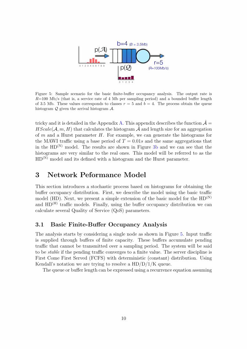
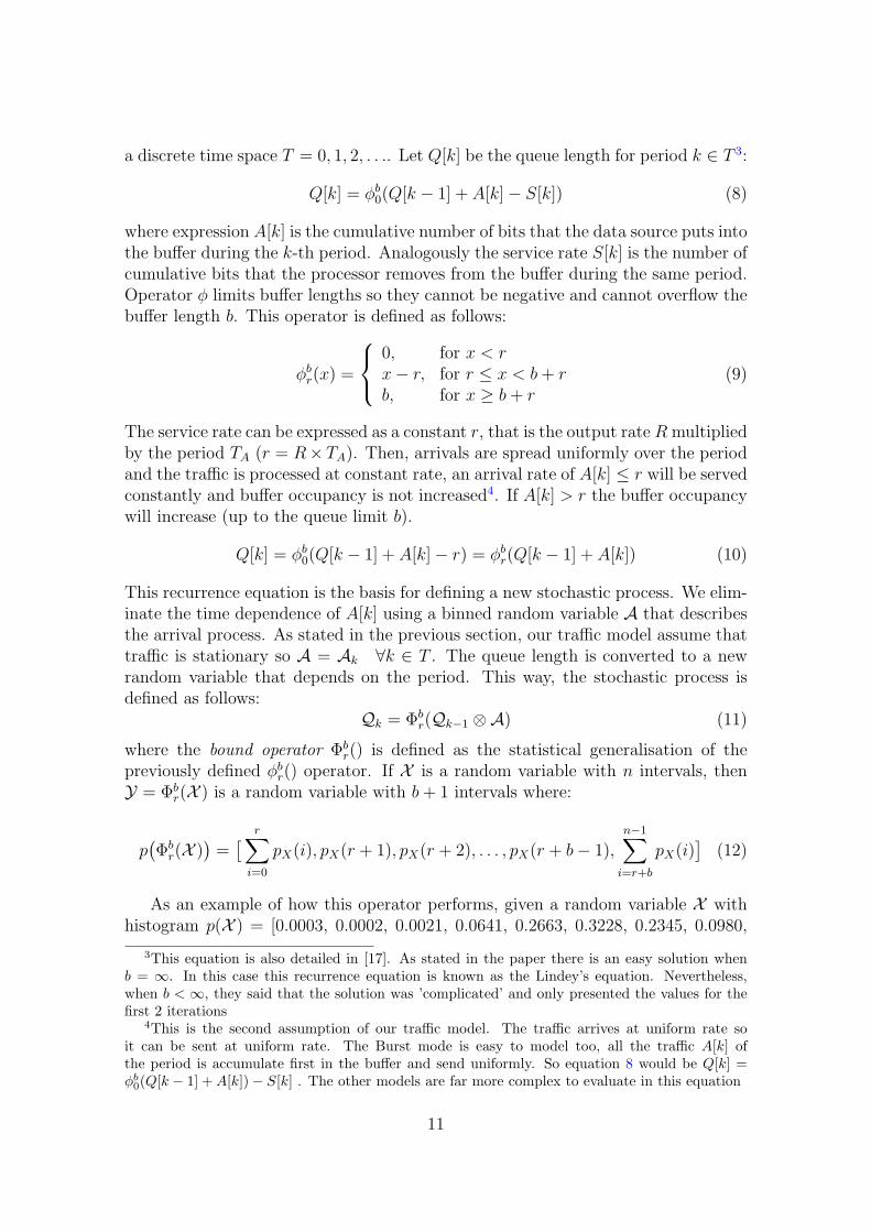
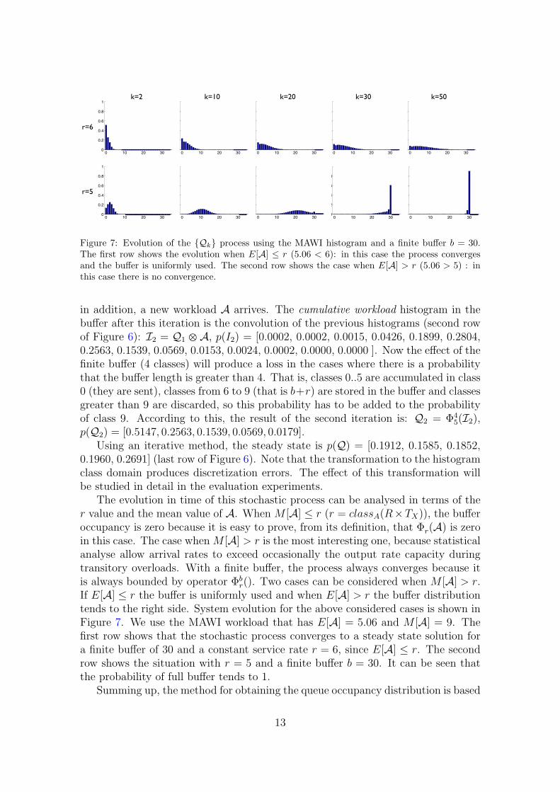
0 10 20 300
02
04
06
08
1
0 10 20 300
02
04
06
08
1
0 10 20 300
02
04
06
08
1
0 10 20 300
02
04
06
08
1
0 10 20 300
02
04
06
08
1
0 10 20 300
02
04
06
08
1
0 10 20 300
02
04
06
08
1
0 10 20 300
02
04
06
08
1
0 10 20 300
02
04
06
08
1
0 10 20 300
02
04
06
08
1
r=6
r=5
k=2 k=10 k=20 k=30 k=50
Figure 7 Evolution of the Qk process using the MAWI histogram and a finite buffer b = 30The first row shows the evolution when E[A] le r (506 lt 6) in this case the process convergesand the buffer is uniformly used The second row shows the case when E[A] gt r (506 gt 5) inthis case there is no convergence
in addition a new workload A arrives The cumulative workload histogram in thebuffer after this iteration is the convolution of the previous histograms (second rowof Figure 6) I2 = Q1 A p(I2) = [00002 00002 00015 00426 01899 0280402563 01539 00569 00153 00024 00002 00000 00000 ] Now the effect of thefinite buffer (4 classes) will produce a loss in the cases where there is a probabilitythat the buffer length is greater than 4 That is classes 05 are accumulated in class0 (they are sent) classes from 6 to 9 (that is b+r) are stored in the buffer and classesgreater than 9 are discarded so this probability has to be added to the probabilityof class 9 According to this the result of the second iteration is Q2 = Φ4
5(I2)p(Q2) = [05147 02563 01539 00569 00179]
Using an iterative method the steady state is p(Q) = [01912 01585 0185201960 02691] (last row of Figure 6) Note that the transformation to the histogramclass domain produces discretization errors The effect of this transformation willbe studied in detail in the evaluation experiments
The evolution in time of this stochastic process can be analysed in terms of ther value and the mean value of A When M [A] le r (r = classA(RtimesTX)) the bufferoccupancy is zero because it is easy to prove from its definition that Φr(A) is zeroin this case The case when M [A] gt r is the most interesting one because statisticalanalyse allow arrival rates to exceed occasionally the output rate capacity duringtransitory overloads With a finite buffer the process always converges because itis always bounded by operator Φb
r() Two cases can be considered when M [A] gt rIf E[A] le r the buffer is uniformly used and when E[A] gt r the buffer distributiontends to the right side System evolution for the above considered cases is shown inFigure 7 We use the MAWI workload that has E[A] = 506 and M [A] = 9 Thefirst row shows that the stochastic process converges to a steady state solution fora finite buffer of 30 and a constant service rate r = 6 since E[A] le r The secondrow shows the situation with r = 5 and a finite buffer b = 30 It can be seen thatthe probability of full buffer tends to 1
Summing up the method for obtaining the queue occupancy distribution is based
13
0
1
0 1 2 3 40
1
0 1 2 3 4 5 6 7 8 9
Histogram Process
R = 100Mbs B = 35 Mb T = 4ms r = 5 b = 4
2
2
3
14
Qk = Φbr(Qkminus1 otimesA)
Figure 8 The HBSP Method for obtaining the buffer distribution (1) The histogram is obtainedfor a traffic workload using a sampling period TA The interval length (lA) is calculated usingthe number of classes and the sample size Smax (2) For a given output rate R and buffer sizeB we obtain the corresponding classes b and r Using the arrival histogram A with the b and rparameters we can apply the stochastic process (3) The steady state of this stochastic process isthe buffer distribution Q Note that the stochastic process only works with classes (4) From thebuffer histogram we obtain the midpoints and represent it using a line graph Using this kind ofgraph is better for comparing several data sets
on this stochastic process This method will be named the HBSP (Histogram BasedStochastic Process) method and is outlined in Figure 8
32 Histogram classes and precision
One key issue is to determine the number of classes of a histogram This is ingeneral a trade off between representation economy and precision If there are toomany intervals the representation will be cumbersome and histogram processingwill be expensive as the complexity of algorithms mostly depends on the number ofclasses On the other hand too few intervals may result in losing information aboutthe distribution and masking trends in data The experiments shows that 10 classesare enough to obtain accurate results
Another important problem is that histogram processing using a reduced numberof classes produces results that has poor precision It is paradoxical that theseerrors occur even if a small number of classes is sufficient to properly describe agiven workload without losing a great deal of information The reason for theseinaccuracies seems to be the effect of the low number of classes when using theiterative algorithms The number of classes for the histogram of the buffer is b+ 1If b is very low (for example 2 or 3) we have only 3 or 4 classes for the resultingbuffer so the precision is very low The solution proposed in this paper consists inoverclassing the histogram
14
Overclassing X by a factor k means applying a transformation ∆+k X minusrarr Y to
increase uniformly the number of classes of X by splitting each interval of X intok intervals of Y The interval length of Y is lY = lXk and its pmf has a largernumber of classes m = ktimesn Probabilities pY(j) are obtained by linear interpolationof values pX (i) in the range i 0 n minus 1 to the range j 0 m minus 1 This wayif we overclass the arrival histogram by a factor of 10 the classes for b will also beincreased by a factor of 10 and the resulting buffer histogram will have more classesand the results will be more accurate In practical terms the experiments show thatthe best results are obtained using over 10 or 20 classes with an overclassing factorof 10
33 Buffer analysis for HD(N) and HD(H) models
In subsection 31 we have described a method to obtain the finite buffer distributionhistogram using the traffic histogram (that is the HDD1K queue solution) Thesolution for the buffer analysis of the HD(N) and HD(H) models is simple and effectivefirst we obtain the buffer histogram for each aggregated histogram and then usingthese buffer histograms we calculate the mean histogram
For the HD(N) model we have a set of h histograms ~A = A(m1)A(m2) middot middot middot A(mh)Using the HDD1K queue solution we can obtain a set of buffer histograms ~Q =Q(m1)Q(m2) middot middot middot Q(mh) The resulting histogram Q will be a function of this set
of histograms ( ~Q) We experimented with several functions and the best approachwas the mean histogram (for the interval length lQ we can use lQ(m1))
p(Q) = [pQ(i) =hsumj=1
pQ(mj)(i)h i = 0 nminus 1] (13)
In the HD(H) model we do not have a set of histograms but we can generate themusing the HScale function described in subsection 22 First we must select theset of values for ~m = m1m2 middot middot middotmh Using this set of values we obtain a set of
histograms ~A = HScale(Ami H) i = 1 h Then we can follow the methodas detailed for the HD(N)model The problem is the selection of the values for mThis will be studied in the evaluation section
34 QoS parameters
Some of the most important performance parameters of a router are delay and lossratio This section shows how to obtain these parameters using the resulting bufferhistogram (Q)
The router delay D is the time between message arrival at that station andmessage departure from the station It is the sum of the queuing delay U and thetransmission delay T This can be expressed in statistical terms as
D = U otimes T (14)
15
The queueing delay is the time spent by the message waiting for previous bufferedmessages to be transmitted In the case of a router with an output rate of R and abuffer length characterized by random variable Q the queueing delay is proportionalto Q so it has the same histogram
U =1
Rmiddot Q (15)
In statistical terms multiplyingQ by a scalar 1R (scalar multiplication) only affectsits interval length Then the interval length of U is lU = lQR expressed in seconds
The transmission delay is the time spent by the network interface in processingthe message and it is closely related to the transmission speed Assuming Td is thedelay for any transmission unit of size lesser than the MTU (Maximum TransmissionUnit) and using the same interval length of U we obtain the class interval as d =classU(Td) In statistical terms T has the following distribution p(T )=[t0 td]with ti = 0 for i le d and ti = 1 for i = d Then D = U otimes T can be calculatedconvolutioning Q and T
D = Qotimes [0 0 1d] (16)
As an example consider the buffer length Q obtained for the histogram used insubsection 31 using a service rate R = 100 Mbs (r = 5) and assume that thetransmission delay is Td = 20 ms First we obtain the interval length of U as lU =lAR = 08100 = 8 ms The class of Td is d = classU(20 ms) = 2 The router delayis calculated as D = QotimesT that is p(D) = [01912 01585 01852 01960 02691]otimes [001] = [0 0 01912 01585 01852 01960 02691] Obtaining the midpoints ofD we have [ 4ms 12ms 20ms 28ms 36ms 44ms 52ms] That means for examplethat probability for 20ms delay (third interval) is about 01912
The calculus of the loss ratio can be clearly understood using the same exampleConsider the stationary cumulative workload pmf (I = Q A p(I)= [0000100001 00005 00127 00616 01163 01584 01851 01960 01528 00844 0028600031 00001]) With a service rate class r = 5 and a buffer length class b = 4from a workload of 13 units 5 units are sent 4 units are stored in the buffer and 4units are lost Therefore the histogram pmf (C) can be obtained by shifting (withaccumulation) r + b = 5 + 4 = 9 positions to the right Using the bound operator
C = Φ9(I) p(C) = [08836 00844 00286 00031 00001] (17)
Histogram C reflects that 08836 is the probability of no loss 00844 is the probabilitythat 1 unit is lost and 00286 is the probability that 2 units are lost and so onAccordingly the probability of at least 1 unit being lost is the following weightedsum E[C] = 00844 lowast 1 + 00286 lowast 2 + 00031 lowast 3 + 0001 lowast 4 = 01513 Then theloss ratio is the proportion between all the units that are lost and the mean of thearrival workload
PL(b) =E[C]E[A]
=01513
506= 299 (18)
16
0 1 2 3 4 5 6 7 8 9 10x 10
5
10minus2
10minus1
100
bits in buffer
prob
abili
ty
HDHD(m)HD(H)Simulation
(a) Queue Probability distribution
0 1 2 3 4 5 6 7 8 9 10x 10
5
0
02
bits in buffer
cum
ulat
ive
prob
abili
ty (
cdf)
HDHD(m)HD(H)Simulation
(b) Cumulative probability (cdf)
Figure 9 Results of the evaluation using MAWI Traffic trace for R = 110 Mbs and B = 1 MbAll the models has 10 classes with an overclassing factor of 10 The HD model has period 40msthe HD(N) model 3 periods (10ms 50ms 200ms) and the HD(H) model a base period of 10ms andm ranging from 1 to 100 (10ms to 1s) The results are very near to the simulated ones The bestresults are obtained using the HD(H) model
4 Evaluation
This section presents an evaluation aimed to validate the models presented in thispaper The best way to validate a performance model is to compare the predictedresults (buffer occupancy distribution and loss ratio) with the ones obtained usingreal traffic traces and real network models We compare the results obtained ana-lytically using the 3 models (HD HD(N) and HD(H)) with results obtained throughsimulation The traffic used in these evaluations are the MAWI trafic [16] trace de-scribed in Figure 1 and the Caida OC-48 traffic [18] The CAIDA OC48 is a packetheader trace of an OC48 link at AMES Internet Exchange (AIX) on Apr 24 2003(1 hour) with an average rate of 92 Mbs
41 Evaluating the traffic models
In order to evaluate that the models are accurate and realistic and event driven sim-ulation using these real traffic trace was performed In each period the simulationcalculates the buffer length and the number of lost packets
In the first experiment we used the MAWI traffic trace (see Figure 1a) the outputrate was set to aproximately the mean rate R = 110 Mbs and the buffer length wasset to B = 1 Mb The parameters r and b are obtained as r = classA(110 Mbstimes004 s) = classA(44 Mb) and b = classA(B) = classA(1 Mb) For example for10 classes (lA = 08 Mb) r = 5 and b = 1 and for 100 classes (lA = 008 Mb) r =50 and b = 12 We obtained analytically the buffer histograms using the followingtraffic models a) an HD model with 10 classes and period 40ms (as shown inFigure 1b) b) the HD(N) model with three sample periods (10ms 50ms 200ms)and c) the HD(H) model with a base period of 10ms and m ranging from 1 to 100
17
0 1 2 3 4 5 6 7 8 9 10x 10
5
10minus3
10minus2
10minus1
100
bits in buffer
prob
abili
ty
HDHD(m)HD(H)Simulation
Figure 10 Queue Probability Distribution using the CAIDA OC-48 traffic trace for R = 90 Mbsand B = 1 Mb The HD(N) model is the most accurate
(10ms to 1s) For the histograms we used 10 classes with an overclassing factorof 10 For comparison we obtained the buffer histogram using simulation Thequeue probability distribution is shown in Figure 9a (note that the y-axe is in logscale) We can appreciate better the differences using the cumulative probability(see Figure 9b) The results for the three models are very accurate although bestresults are obtained using the HD(N) model Regarding the loss ratio the simulationprovided a value of 00640109 while the HD model estimated a value of 0041934the HD(N) model 00576173 and 00583313 for the HD(H) model
For the following experiment we used the CAIDA OC-48 traffic The outputrate was set to R = 90 Mbs and the buffer length was set to B = 1 Mb Weobtained analytically the buffer histograms using the same sample periods for thetraffic models of the MAWI experiments The results are in Figure 10 We can seethat the best results are obtained using the HD(m) model Regarding the loss ratiothe simulation provided a value of 00494095 while the HD model estimated a valueof 00344655 the HD(N) model 00436831 and 00426831 for the HD(H) model
Previous experiments used a 1-hour trace for obtaining the histogram producingvery good results The following experiment uses the MAWI 12-hour trace (from800 to 2000 of the Jan 09 2007 traces) The rate was set to R = 120 Mbs and thebuffer length to B = 1 Mb This means using long-term traces instead of short-termtraces Results are still very accurate as shown in Figure 11 Regarding the lossratio the HD model predicted 00146371 HD(N) 00214733 and HD(H) 00202713while the simulation yielded 00275981 In summary there is a little loss of accuracywhen using long-term traces as it could be expected due to information loss in thehistogram representation
Previous experiments were also repeated with different traffic traces (using MAWItraces from a different day and hour and traces from the NLANR repository) out-put rates and buffer lengths Results were very similar to the ones presented here(See [19] for more experiments)
18
0 1 2 3 4 5 6 7 8 9 10x 10
5
10minus3
10minus2
10minus1
100
bits in buffer
prob
abili
ty
HDHD(m)HD(H)Simulation
Figure 11 MAWI long-term traffic queue distribution for R = 120 Mbs and B = 1 Mb Theresults of using a 12-hour trace are still very accurate
42 Accuracy
This subsection is devoted to identify and evaluate factors that may affect the ac-curacy of the results The selection of the number of classes and the sample periodwas based on the results of the following experiments
One of the keys aspect of these traffic models is the selection of the sampleperiods We analyse the relation between the sampling period and accuracy usingthe basic HD model In Figure 12a is the result of obtaining the buffer histogramfor several sample periods (base period = 10ms m = 1 2 5 10 100 ) We cansee that the precision is clearly affected by the sample period The best results areobtained using m = 5 that is a sampling period of 50ms Figure 12b shows thenormalized difference5 between the buffer histograms obtained using the HD trafficand that obtained through simulations varying the sample rate from 10ms to 20sThis figure also shows the loss ratio error that is the relative error between theloss ratio predicted by our model and the ones obtained in the simulation The bestprecision is obtained using periods between 20ms and 100ms
The following experiment analyses the relation between buffer length and lossratio for the HD(N) traffic model Loss ratios are calculated for different output ratesvarying the buffer length between 10 kb and 10 Mb (this corresponds to a maximalqueue delay of less than 01 s) Results are presented in the form of a loss ratiocurve (see Figure 13) The prediction of loss rate using the HD(N) traffic model isvery accurate since it is very close to simulations
Regarding on the number of classes several experiments were done varying thenumber of histogram classes The key question is how many classes are necessary toget a good accuracy In the following experiment the number of classes was variedfrom 6 to 100 and 4 histograms were calculated the first one using the originalhistogram with no overclassing and the other 3 using overclassing factors of 5 10and 20 The normalized difference between these histograms and the one obtained
5the normalized difference of 2 vectors A=[a1 middot middot middot an] and B=[b1 middot middot middot bn] is defined asradic(a1 minus b1) + middot middot middot+ (an minus bn)
19
0 1 2 3 4 5 6 7 8 9 10x 10
5
10minus06
10minus05
10minus04
10minus03
10minus02
10minus01
bits in buffer
cum
ulat
ive
prob
abili
ty (
cdf)
HD(1)HD(2)HD(5)HD(10)HD(100)Simulation
(a)
10minus2
10minus1
100
1010
005
01
015
02
025
03
period (s)
Diff
eren
ce
Histogram differenceLoss ratio error
(b)
Figure 12 Sample Period and precision a) Queue Probability distribution for several sampleperiods (base period = 10ms) We can see the precision of the result depends clearly on the baseperiod b) This graph shows the Normalized difference between the histograms and the loss ratioerror obtained using the HD model and the simulations for sample rate between 10ms and 20sThe best results are obtained for periods between 20ms and 100ms
0 1 2 3 4 5 6 7 8 9 10
x 106
0
002
004
006
008
01
012
buffer
Histogram R=100MbsSimulation R=100MbHistogram R=120MbSimulation R=120MbsHistogram R=150MbsSimulation R=150Mbs
Figure 13 Loss Ratio Curve the loss ratio is obtained for the the HD(N) model and is comparedto the results obtained in the simulation using different output rates (R=100 110 and 120 Mbs)and varying the buffer length The results are very accurate for R=100Mbs For R=120Mbsthere is a loss of precision in some ranges
20
0 20 40 60 80 100
1
05
classes
norm
aliz
ed d
iffer
ence
x1x5x10x20
(a) Normalized difference for R = 110Mbs B = 1Mb
0 20 40 60 80 100009
01
011
012
013
014
015
016
017
classes
cell
loss
rat
io
x1x5x10x20Simulation
(b) Cell loss ratio for R = 100Mbs B = 1Mb
Figure 14 Relation between Number of Classes overclassing and precision the number of classeswas varied from 6 to 100 and 4 histograms were calculated rsquox1rsquo original histogram rsquox5rsquorsquox10rsquo andrsquox20rsquo with overclassing factors of 5 10 and 20 We can see that accuracy is not greatly improvedusing more than 15 classes and better results are obtaining using an overclassing factor of 10
through simulation is shown in Figure 14a The loss ratio is compared with the lossratio of simulations in Figure 14b Results show that the main effect of overclassingis to smooth the results reducing the original peaks It can be also seen that thereis no significant variation using a overclassing factor greater than 10 Regarding onthe number of original classes it can be seen that accuracy is not greatly improvedusing more than 15 of 20 classes For the original histogram accuracy is betterin some cases using more than 60 classes (see Figure 14a) but in some other casesit is worst Therefore in the average case it is better to use overclassing Thefinal conclusion is that the best results are obtained using 10 to 20 classes with anoverclassing factor of 10
43 Long-range dependence implications on the models
In [17] is discussed the impact of the long-range dependence (LRD) on the bufferoccupancy and indicated that LRD does not affect the buffer occupancy when thebusy periods of the system are not large Similar conclusions were obtained in [20]short-term correlation have dominant effect on cell loss ratio More important is tochoose the critical time scale (CTS) that is related with the sample period In [20]the authors considered the buffer behavior at the time-scale beyond the CTS is nosignificantly affected The experiments of this paper showed that the best modelwas HD(N) that is not strictly LRD Therefore the results confirms the results of [20]and [17] Our experiments shows that when selecting correctly the sampling periodthe results are very accurate
Another question is the selection of the model Each model has its pros andcons
bull HD model this model is simple and compact and the results are still veryaccurate It is a good approximation
21
0 1 2 3 4 5 6 7 8 9 10x 10
5
10minus4
10minus3
10minus2
10minus1
100
bits in buffer
prob
abili
ty
HD(m) modelHistogram MD1K methodPacket Simulation
(a)
0 05 1 15 2 25 3 35 4 45 5x 10
6
003
004
005
006
007
008
009
01
011
012
buffer
simulationHD(M) modelMVA
(b)
Figure 15 Comparison with other methods a) Comparison of the buffer histograms obtainedusing our HD(N) model and the MD1K approach by Skelly and Shroff ( [12] for R = 110Mbs B= 1Mb We can see that the MD1K approach collapses when the buffer is large b) Comparison ofthe cell loss ratio obtained using the Maximum Variance Asymptotic (MVA) method versus theHD(N) model results R = 110Ms The graph shows a better precision of the HD(N) model
bull HD(N) it is the more accurate model but it is not so compact We must obtainseveral histograms for several periods so it can be cumbersome
bull HD(H) this model is still compact (we only need one histogram and the Hurstparameter) and the results are very good
44 Comparison with other methods
This section compares the model with previously published methods for analyzingbuffer length and loss ratio To simplify we only compare the results of the HD(N)
model Regarding the calculation of the buffer length the best known approach isthe method introduced by Skelly and Shroff (known as the Histogram Model [12]or the Generalized Histogram Model [13] and used with few modifications in [21]and [22]) This approximation is based on resolving an MD1N queue for eacharrival rate of the histogram We implemented this method and compared theobtained buffer length histogram with the one obtained using the HD(N) modelFigure 15a shows that the differences between the HBSP model and the MD1Nmethod are large The results using the MD1N are imprecise The problemswith the MD1N is that the buffer curve collapses when the buffer size if highThe results presented in [12] used very low buffer lengths (about 50 cells) so theresults were more accurate Nevertheless when larger buffer (about 500) the buffercurve begins to collapse
Regarding the loss ratio most of the papers deal with the tail probability (oroverflow probability) P (Q gt t) rather than the loss probability In this paperwe compare the HBSP method versus the Maximum Variance Asymptotic (MVA)approximation for loss detailed in [11] In Figure 15b we can see the loss probability
22
Ingress
node1
Egress
node 2 node 3
node 6
node 5
node 4
node 7
Channel
0
3
0 1 2 3 4
0
3
0 1 2 3 4
0
3
0 1 2 3 4
0
7
0 1 2 3 4
0
3
0 1 2 3 4
0
4
0 1 2 3 4
0
3
0 1 2 3 4
0
4
0 1 2 3 4
0
4
0 1 2 3 4
Figure 16 Sample network with the load histograms of the nodes This can be seen as a visualmonitorization of the network load With this information we can obtain the loss ratio the end-to-end delay distribution for a given path
depending on the buffer size The graph shows that the HD(N) cell loss curve is moreprecise than the MVA curve
5 Applications of the model
There is a wide spectrum of applications of the HBSP model We can obtain thetraffic QoS parameters as loss ratio or node delay using the HBSP model Usingthe router delay of the nodes we can obtain the network delay pmf DN This pmfis obtained as the sum (convolution) of the node pmfs that a packet traverses
DN =otimesiisinpath
Di (19)
For example using Figure 16 we can obtain the end-to-end delay distribution forthe path marked with blue This pmf is very useful because we can obtain the meandelay or for example the probability that a packet is delayed more than a certainvalue For example if we transmit video or audio the delay histogram can be usefulin the end nodes to adapt their transmissions rates or to configure the buffer in thereception nodes This information can be used for admission control as well
Another important application is for traffic provisioning and network configura-tion Optimal provisioning of network resources is crucial for reducing the servicecost of network transmission This is the goal of Traffic Engineering the designprovisioning performance evaluation and tuning of operational networks The fun-damental problem with provisioning is to have methods and tools to decide the net-work resource reservation for a given Quality of Service requirements [23] Thereforethe HBSP method can be very useful for Traffic Engineering The HBSP methodallows to obtain the load histogram of the nodes of a network These histograms canbe used to configure the network For example if we have a network like the one
23
presented in Figure 16 we can see that node 4 is highly loaded and we can decide toincrease its resource or to change some route in order to reduce the load in node 4
It also allows to evaluate parameters like the loss ratio (for a given buffer andoutput ratio) the node delay the bufferoutput ratio needed for a required loss etcOne important decision that must be taken is the time-scale of the provisioning Themeasured traffic can be a long-term trace (daily or weekly traces) or a short-termtrace (hourly traces) This depends on the network capability to support dynamicalvariation in the reservation of the channel resources (for example an hour) (see [24])
A great advantage of the HBSP model is the easy implementation of the his-tograms Is very easy to capture and store a load histogram with few classes (about10) in a network node
6 Conclusions
This paper introduces three traffic models and a performance model to obtain thefinite buffer occupancy distribution The performace model is based on a stochasticprocess working with histograms for resolving the HDD1K queue The resultof this stochastic process is a histogram of the buffer distribution This bufferdistribution has an easy solution for the infinite buffer case but it seems to havea complicated solution for the finite buffer case [17] For this reason most of thepapers obtains the tail probability P (Q gt t) using an infinite buffer model andapproximate the cell loss using this tail probability The model presented in thispaper is a solution of the finite buffer case From the buffer histogram and thearrival histogram it is easy to obtain the cell loss ratio
Three models are described in this paper The first model (HD) is a basichistogram model that is compact and short-range dependent The second one (theHD(N) model) is based on obtaining several histograms using different time scalesThe third one (the HD(H) model) is based on the Hurst parameter and it is long-range dependent Experiments were performed using several real-traffic traces Thebest results are obtaining using the HD(N) model although it can be cumbersomeSo the best approach is the HD(H) model that is compact and it is very precise
There is a wide spectrum of applications of this model We can obtain the trafficQoS parameters as loss ratio or node delay The delay histogram is very usefulbecause we can obtain the mean delay or for example the probability that a packetis delayed more than a certain value For example if we transmit video or audio thedelay histogram can be useful in the end nodes to adapt their transmissions ratesor to configure the buffer in the reception nodes This information can be used foradmission control as well Another important application is for traffic provisioningand network configuration Optimal provisioning of network resources is crucial forreducing the service cost of network transmission
24
7 Acknowledgments
This work was developed under grants of the Generalitat Valenciana (GV2007192)and the Spanish Government (CICYT TIN2005-08665-C03-03)
References
[1] Ronald G Addie Moshe Zukerman and Timothy D Neame Broadband trafficmodeling Simple solutions to hard problems IEEE Communications Magazinepages 88ndash95 August 1998
[2] Will E Leland Murad S Taqqu Walter Willinger and Daniel V Wilson On theself-similar nature of ethernet traffic (extended version) IEEEACM Trans Netw2(1)1ndash15 1994
[3] Vern Paxson and Sally Floyd Wide area traffic the failure of poisson modelingIEEEACM Trans Netw 3(3)226ndash244 1995
[4] Jin Cao William S Cleveland Dong Lin and Don X Sun Nonlinear Estimationand Classification chapter Internet Traffic Tends Toward Poisson and Independentas the Load Increases Springer 2002
[5] E Casilari JM Cano-Garcia FJ Gonzalez-Canete and F Sandoval Modellingof individual and aggregate web traffic In IEEE International Conference on HighSpeed Networks and Multimedia Communications HSNMC pages 84ndash95 2004
[6] P Abry R Baraniuk P Flandrin R Riedi and D Veitch Multiscale nature ofnetwork traffic IEEE Signal Processing Magazine 19(3)28ndash46 2002
[7] David L Jagerman Benjamin Melamed and Walter Willinger Stochastic modelingof traffic processes pages 271ndash320 1997
[8] David M Lucantoni The BMAPG1 queue A tutorial In Performance Evaluationof Computer and Communication Systems Joint Tutorial Papers of Performance rsquo93and Sigmetrics rsquo93 pages 330ndash358 London UK 1993 Springer-Verlag
[9] Alexander Klemm Christoph Lindemann and Marco Lohmann Modeling ip trafficusing the batch markovian arrival process Performance Evaluation 54149ndash173 2003
[10] On Hassida Yoshitaka Takahashi and Shinsuke Shimogawa Multiscale nature ofnetwork traffic Switched Batch Bernoulli Process (SBBP) and the Discrete-timeSBBPG1 queue with Application to Statistical Multiplexer Performance 9(3)394ndash401 1991
[11] Han S Kim and Ness B Shroff On the asymptotic relationship between the overflowprobability and the loss ratio IEEEACM Trans Netw 9(6)755ndash768 2001
[12] P Skelly M Schwartz and S Dixit A histogram-based model for video trafficbehavior in an ATM multiplexer IEEEACM Transactions on Networking 1(4)446ndash459 August 1993
25
[13] Ness B Shroff and Mischa Schwartz Video modeling withing networks using deter-ministic smoothing at the source In IEEE Infocom pages 342ndash349 1994
[14] J Luthi S Majumdar and G Haring Mean value analysis for computer systemswith variabilities in workload In IPDS rsquo96 Proceedings of the 2nd InternationalComputer Performance and Dependability Symposium page 32 Washington DCUSA 1996 IEEE Computer Society
[15] Moshe Zukerman Timothy D Neame and Ronald G Addie Internet traffic modelingand future technology implications In IEEE Infocom 2003
[16] K Cho and et al Traffic data repository at the wide project In USENIX 2000FREENIX Track 6 2000
[17] Daniel P Heyman and T V Lakshman What are the implications of long-rangedependence for VBR-video traffic engineering IEEEACM Trans Netw 4(3)301ndash317 1996
[18] DatCat Caida oc48 traces 2003-04-24 download in httpimdcdatcatorg
[19] E Hernandez and JVila A stochastic analysis of network traffic based on histogramworkload modelling Technical Report UPV-DISCA-06-09 September 2006 Down-load in httpwwwdiscaupvesenherorpdfTR_DISCA_06_09pdf
[20] Bong K Ryu and Anwar Elwalid The importance of long-range dependence of VBRvideo traffic in ATM traffic engineering myths and realities In SIGCOMM rsquo96pages 3ndash14 New York NY USA 1996 ACM Press
[21] Ness B Shroff and M Schwartz Improved loss calculations at an ATM multiplexerIEEEACM Transactions on Networking 6(4)411ndash21 August 1998
[22] Seok-Kyu Kweon and Kang G Shin Real-time transport of MPEG video with astatistically guaranteed loss ratio in ATM networks IEEE Transactions In Paralleland Distributed Computing 12(4)387ndash403 April 2001
[23] D Awduche and et al Overview and principles of internet traffic engineering RFC3272 May 2002
[24] Enrique Hernandez-Orallo Joan Vila-Carbo Sergio Saez-Barona and Silvia Terrasa-Barrena Provisioning expedited forwarding diffserv channels using multimedia ag-gregates In Euromicro 2004 9 2004
A Method for scaling and histogram
This appendix describes how to obtain the m-aggregated histogram A with a vari-ance according to the scaling function m2Hminus2 The function that obtains this newhistogram will be named HScale That is A = HScale(AmH) generates a newhistogram A with variance m2Hminus2 middotV ar(A) pmf p(A) = [pA(i) i = 0 nminus 1] andinterval length lA middotm
26
As the variance of A must be reduced we are going to shrink the histogramFor example if we have the histogram p(A) = [02 06 02] that has mean 1 andvariance 04 and we want to decrease its variance to 03 the new histogram will be[015 07 015]
The goal is to shrink the histogram reducing the values at the edges and ac-cumulating this reduction for the classes in the mean Assume that the histogramhas n classes and the classes in the mean are h = bE(A)c and h + 1 We startin the left edge The probability of class 0 (p0 = pA(0)) is reduced by a factor c(05 lt c lt 1) That is p0 = pA(0) = c middot p0 This reduction ((1 minus c) middot p0) is accu-mulated to class 1 that is also reduced by c p1 = c middot p1 + (1 minus c) middot p0 For classhminus 1 we have phminus1 = c middot phminus1 + (1minus c) middot phminus2 For the classes in the mean we mustcalculate another reducing factor cprime The reason is to reduce these classes accordingto the mean For example if the mean is very near the class h we must reduce theclass h + 1 accordingly On the other hand if the mean is near to class h + 1 wemust reduce the class h This factor is obtained as cprime = 05minus (hminus E(A)) Assumecprime gt 0 (mean near class h) then we have ph = ph + (1 minus c) middot phminus1 + cprime middot ph+1 andph+1 = (1minuscprime) middotph+1 +(1minusc) middotph+2 For cprime lt 0 is similar The right side is equivalentto the left So we have
p0 = c middot p0 = p0 middot cp1 = c middot p1 + (1minus c) middot p0 = p0 + (p1 minus p0) middot c
phminus1 = c middot phminus1 + (1minus c) middot phminus2 = phminus2 + (phminus1 minus phminus2) middot cph = ph + (1minus c) middot phminus1 + cprime middot ph+1 = ph + phminus1 + cprime middot ph+1 + minusphminus1 middot cph+1 = (1minus cprime) middot ph+1 + (1minus c) middot ph+2 = (1minus cprime) middot ph+1 + ph+2 + minusph+2 middot cph+2 = c middot ph+2 + (1minus c) middot ph+3 = ph+3 + (ph+2 minus ph+3) middot c
pnminus1 = c middot pnminus1 = pnminus1 middot c(20)
It is easy to see thatsumnminus1
0 pi = 1The goal of the following method is to transform a histogram A to a scaled
histogram A with variance v = m2Hminus2 middot V ar(A) We have
V ar(A) =nminus1sum
0
(iminus E[A])2︸ ︷︷ ︸di
middotpi =nminus1sum
0
di middot pi = v (21)
Then we multiply all the terms in equation 20 by di and summing all the probabil-ities and grouping terms we have
sumnminus10 di middot pi = Sc middot c+ S = v (the SA coefficient is
the sum of all the coefficients of the c variable and SB is the sum of the coefficientswithout variable) Then the reducing factor c is obtained as
c =v minus SSc
(22)
27
For obtaining the coefficients we must obtain the values of di We need to estimatethe value of E[A] The mean of the original histogram (E[A]) is a good estimatorUsing this mean we obtain the sum of the coefficients and resolve equation 22 Withthis factor c we apply equations 20 for obtaining the distribution of A Normallythe variance of A will not be exactly v because we are estimating the mean as E[A]So we can repeat the calculations using the mean of the calculated histogram E[A]Practically in 2 or 3 iterations we obtain the desired histogram with the requiredvariance If the result of c is not in the range 05 lt c lt 1 this mean that the desiredvariance can not be obtained in one step So we apply a factor of 05 to obtain anew histogram that is shrunk by a factor of 05 and using this new histogram wecan obtain a new factor c until the factor is greater than 05
The algorithm of the HScale function is outlined in Figure 17 In the algorithmwe have 2 functions The function SumCoef obtains the sum of the coefficients SAand SB for a given mean and the function Getpmf calculate the pmf according toequation 20
As an example of how the function works we will use the MAWI histogram ofFigure 1b p(A) = [00003 00002 00021 00641 02663 03228 02345 0098000110 00005] that has a base period of 004ms variance 1282 and an intervallength of lA = 008Mb For m = 10 and H = 085 the result is p(A) = [0000100002 00010 00289 01478 06580 01105 00481 00050 00002] with an inter-val length of 8Mb The variance is 06334 according to v = var(A) middotm2Hminus2
B Buffer analysis as a DTMC
In this appendix we show that the stochastic process Qk is a Discrete-Time MarkovChain (DTMC) Additionally we can easily obtain the transition probability matrixP Using this probability matrix we can obtain the values for Qk The problem ofusing DTMC it that is not easy to obtain an analytical solution for the steady state(that is when k rarrinfin)
A Discrete-Time Markov Chain is a stochastic process whose probabilities distri-butions in state j only depends on the previous state i and not on how the processarrived to state i It is easy to proof that Qk is a DTMC The probability that thebuffer in period k takes the value j can be expressed using the buffer probabilitiesof period k minus 1 as follows
P [Qk = j] =sumi
P [Qkminus1 = i] middot P [Qk = j|Qkminus1 = i] (23)
The term pij(k minus 1 k) = P [Qk = j|Qkminus1 = i] denotes the probability that theprocess makes a transition from state i at period k minus 1 to state j at period k Thisprobability is obtained from the arrival load A and given that A is the same in allthe periods then the pij(k minus 1 k) does not depend on the period k Therefore wecan represent pij(k minus 1 k) as pij and Equation 24 is reduced to
P [Qk = j] =sumi
P [Qkminus1 = i] middot pij (24)
28
Algorithm A = HScale(A m H)inputA rsquoOriginal histogramm rsquoAggregationH rsquoHurst parameteroutputA rsquoHistogram for the m-aggregation
1 begin3 v = V ar(A) middotm(2minus2H)Ac = A4 while true5 mean = E[Ac]6 do7 [S Sc] = SumCoef(Ac mean)8 c = (v minus S)Sc9 Af = Getpmf(Ac c mean) rsquoCalculate the pmf for c10 mean = E[Af ] rsquoRepeat with a new mean11 while (05 lt c lt 1) and (|V ar(Af )minus v| lt ε)12 if 05 lt c lt 113 A = Af rsquoThe histogram has Var=v14 return15 else16 mean = E[Ac]17 Ac = Getpmf(Ac 05 mean) rsquoScale the histogram by 0518 end if19 end while20 end
Figure 17 The fv algorithm
29
pij is known as the one-step transition probability From this we can obtain thetransition probability matrix
P = [pij] =
p00 p01 p02 middot middot middotp10 p11 p12 middot middot middot
(25)
The components of this matrix are easy to obtain using the definition of the stochas-tic process Qk That is for obtaining the i-row of P we apply one iteration of thestochastic process using an initial load of one unit in j For example the first rowis obtained as Φb
r([1 0 0 0 ] A) Using the matrix P we can obtain the pmf ofQk as
Qk = Q1Pk (26)
Nevertheless determining the asymptotic behavior (that is the steady state) posesproblems This implies obtaining the steady-state probability vector v as
v = vP vj ge 0sumj
vj = 1 (27)
This matrix has a finite size of (b+ 1)times (b+ 1) Nevertheless numerically resolvingEquation 27 is not easy even for a little matrix Therefore we must use iterativemethods as the power method or something similar
Using the example of subsection 31 p(A) =[00003 00002 00021 0064102663 03228 02345 00980 00110 00005] with r=5 and b=4 we obtain thefollowing matrix
P =
06558 02345 00980 00110 0000503330 03228 02345 00980 0011500667 02663 03228 02345 0109500026 00641 02663 03228 0344000005 00021 00641 02663 06668
(28)
We can obtain the second iteration state as Q2 = Q1P = [05147 02563 0153900569 00179] The steady state probability vector is v = [01912 01585 0185201960 02691] This is the pmf of Q (p(Q))
30
- 1 Introduction
- 2 Traffic Workload Models
-
- 21 Basic Histogram Workload Model
- 22 Second-order Statistics models
-
- 3 Network Peformance Model
-
- 31 Basic Finite-Buffer Occupancy Analysis
- 32 Histogram classes and precision
- 33 Buffer analysis for HD(N) and HD(H) models
- 34 QoS parameters
-
- 4 Evaluation
-
- 41 Evaluating the traffic models
- 42 Accuracy
- 43 Long-range dependence implications on the models
- 44 Comparison with other methods
-
- 5 Applications of the model
- 6 Conclusions
- 7 Acknowledgments
- A Method for scaling and histogram
- B Buffer analysis as a DTMC
-

0
1
0 1 2 3 40
1
0 1 2 3 4 5 6 7 8 9
Histogram Process
R = 100Mbs B = 35 Mb T = 4ms r = 5 b = 4
2
2
3
14
Qk = Φbr(Qkminus1 otimesA)
Figure 8 The HBSP Method for obtaining the buffer distribution (1) The histogram is obtainedfor a traffic workload using a sampling period TA The interval length (lA) is calculated usingthe number of classes and the sample size Smax (2) For a given output rate R and buffer sizeB we obtain the corresponding classes b and r Using the arrival histogram A with the b and rparameters we can apply the stochastic process (3) The steady state of this stochastic process isthe buffer distribution Q Note that the stochastic process only works with classes (4) From thebuffer histogram we obtain the midpoints and represent it using a line graph Using this kind ofgraph is better for comparing several data sets
on this stochastic process This method will be named the HBSP (Histogram BasedStochastic Process) method and is outlined in Figure 8
32 Histogram classes and precision
One key issue is to determine the number of classes of a histogram This is ingeneral a trade off between representation economy and precision If there are toomany intervals the representation will be cumbersome and histogram processingwill be expensive as the complexity of algorithms mostly depends on the number ofclasses On the other hand too few intervals may result in losing information aboutthe distribution and masking trends in data The experiments shows that 10 classesare enough to obtain accurate results
Another important problem is that histogram processing using a reduced numberof classes produces results that has poor precision It is paradoxical that theseerrors occur even if a small number of classes is sufficient to properly describe agiven workload without losing a great deal of information The reason for theseinaccuracies seems to be the effect of the low number of classes when using theiterative algorithms The number of classes for the histogram of the buffer is b+ 1If b is very low (for example 2 or 3) we have only 3 or 4 classes for the resultingbuffer so the precision is very low The solution proposed in this paper consists inoverclassing the histogram
14
Overclassing X by a factor k means applying a transformation ∆+k X minusrarr Y to
increase uniformly the number of classes of X by splitting each interval of X intok intervals of Y The interval length of Y is lY = lXk and its pmf has a largernumber of classes m = ktimesn Probabilities pY(j) are obtained by linear interpolationof values pX (i) in the range i 0 n minus 1 to the range j 0 m minus 1 This wayif we overclass the arrival histogram by a factor of 10 the classes for b will also beincreased by a factor of 10 and the resulting buffer histogram will have more classesand the results will be more accurate In practical terms the experiments show thatthe best results are obtained using over 10 or 20 classes with an overclassing factorof 10
33 Buffer analysis for HD(N) and HD(H) models
In subsection 31 we have described a method to obtain the finite buffer distributionhistogram using the traffic histogram (that is the HDD1K queue solution) Thesolution for the buffer analysis of the HD(N) and HD(H) models is simple and effectivefirst we obtain the buffer histogram for each aggregated histogram and then usingthese buffer histograms we calculate the mean histogram
For the HD(N) model we have a set of h histograms ~A = A(m1)A(m2) middot middot middot A(mh)Using the HDD1K queue solution we can obtain a set of buffer histograms ~Q =Q(m1)Q(m2) middot middot middot Q(mh) The resulting histogram Q will be a function of this set
of histograms ( ~Q) We experimented with several functions and the best approachwas the mean histogram (for the interval length lQ we can use lQ(m1))
p(Q) = [pQ(i) =hsumj=1
pQ(mj)(i)h i = 0 nminus 1] (13)
In the HD(H) model we do not have a set of histograms but we can generate themusing the HScale function described in subsection 22 First we must select theset of values for ~m = m1m2 middot middot middotmh Using this set of values we obtain a set of
histograms ~A = HScale(Ami H) i = 1 h Then we can follow the methodas detailed for the HD(N)model The problem is the selection of the values for mThis will be studied in the evaluation section
34 QoS parameters
Some of the most important performance parameters of a router are delay and lossratio This section shows how to obtain these parameters using the resulting bufferhistogram (Q)
The router delay D is the time between message arrival at that station andmessage departure from the station It is the sum of the queuing delay U and thetransmission delay T This can be expressed in statistical terms as
D = U otimes T (14)
15
The queueing delay is the time spent by the message waiting for previous bufferedmessages to be transmitted In the case of a router with an output rate of R and abuffer length characterized by random variable Q the queueing delay is proportionalto Q so it has the same histogram
U =1
Rmiddot Q (15)
In statistical terms multiplyingQ by a scalar 1R (scalar multiplication) only affectsits interval length Then the interval length of U is lU = lQR expressed in seconds
The transmission delay is the time spent by the network interface in processingthe message and it is closely related to the transmission speed Assuming Td is thedelay for any transmission unit of size lesser than the MTU (Maximum TransmissionUnit) and using the same interval length of U we obtain the class interval as d =classU(Td) In statistical terms T has the following distribution p(T )=[t0 td]with ti = 0 for i le d and ti = 1 for i = d Then D = U otimes T can be calculatedconvolutioning Q and T
D = Qotimes [0 0 1d] (16)
As an example consider the buffer length Q obtained for the histogram used insubsection 31 using a service rate R = 100 Mbs (r = 5) and assume that thetransmission delay is Td = 20 ms First we obtain the interval length of U as lU =lAR = 08100 = 8 ms The class of Td is d = classU(20 ms) = 2 The router delayis calculated as D = QotimesT that is p(D) = [01912 01585 01852 01960 02691]otimes [001] = [0 0 01912 01585 01852 01960 02691] Obtaining the midpoints ofD we have [ 4ms 12ms 20ms 28ms 36ms 44ms 52ms] That means for examplethat probability for 20ms delay (third interval) is about 01912
The calculus of the loss ratio can be clearly understood using the same exampleConsider the stationary cumulative workload pmf (I = Q A p(I)= [0000100001 00005 00127 00616 01163 01584 01851 01960 01528 00844 0028600031 00001]) With a service rate class r = 5 and a buffer length class b = 4from a workload of 13 units 5 units are sent 4 units are stored in the buffer and 4units are lost Therefore the histogram pmf (C) can be obtained by shifting (withaccumulation) r + b = 5 + 4 = 9 positions to the right Using the bound operator
C = Φ9(I) p(C) = [08836 00844 00286 00031 00001] (17)
Histogram C reflects that 08836 is the probability of no loss 00844 is the probabilitythat 1 unit is lost and 00286 is the probability that 2 units are lost and so onAccordingly the probability of at least 1 unit being lost is the following weightedsum E[C] = 00844 lowast 1 + 00286 lowast 2 + 00031 lowast 3 + 0001 lowast 4 = 01513 Then theloss ratio is the proportion between all the units that are lost and the mean of thearrival workload
PL(b) =E[C]E[A]
=01513
506= 299 (18)
16
0 1 2 3 4 5 6 7 8 9 10x 10
5
10minus2
10minus1
100
bits in buffer
prob
abili
ty
HDHD(m)HD(H)Simulation
(a) Queue Probability distribution
0 1 2 3 4 5 6 7 8 9 10x 10
5
0
02
bits in buffer
cum
ulat
ive
prob
abili
ty (
cdf)
HDHD(m)HD(H)Simulation
(b) Cumulative probability (cdf)
Figure 9 Results of the evaluation using MAWI Traffic trace for R = 110 Mbs and B = 1 MbAll the models has 10 classes with an overclassing factor of 10 The HD model has period 40msthe HD(N) model 3 periods (10ms 50ms 200ms) and the HD(H) model a base period of 10ms andm ranging from 1 to 100 (10ms to 1s) The results are very near to the simulated ones The bestresults are obtained using the HD(H) model
4 Evaluation
This section presents an evaluation aimed to validate the models presented in thispaper The best way to validate a performance model is to compare the predictedresults (buffer occupancy distribution and loss ratio) with the ones obtained usingreal traffic traces and real network models We compare the results obtained ana-lytically using the 3 models (HD HD(N) and HD(H)) with results obtained throughsimulation The traffic used in these evaluations are the MAWI trafic [16] trace de-scribed in Figure 1 and the Caida OC-48 traffic [18] The CAIDA OC48 is a packetheader trace of an OC48 link at AMES Internet Exchange (AIX) on Apr 24 2003(1 hour) with an average rate of 92 Mbs
41 Evaluating the traffic models
In order to evaluate that the models are accurate and realistic and event driven sim-ulation using these real traffic trace was performed In each period the simulationcalculates the buffer length and the number of lost packets
In the first experiment we used the MAWI traffic trace (see Figure 1a) the outputrate was set to aproximately the mean rate R = 110 Mbs and the buffer length wasset to B = 1 Mb The parameters r and b are obtained as r = classA(110 Mbstimes004 s) = classA(44 Mb) and b = classA(B) = classA(1 Mb) For example for10 classes (lA = 08 Mb) r = 5 and b = 1 and for 100 classes (lA = 008 Mb) r =50 and b = 12 We obtained analytically the buffer histograms using the followingtraffic models a) an HD model with 10 classes and period 40ms (as shown inFigure 1b) b) the HD(N) model with three sample periods (10ms 50ms 200ms)and c) the HD(H) model with a base period of 10ms and m ranging from 1 to 100
17
0 1 2 3 4 5 6 7 8 9 10x 10
5
10minus3
10minus2
10minus1
100
bits in buffer
prob
abili
ty
HDHD(m)HD(H)Simulation
Figure 10 Queue Probability Distribution using the CAIDA OC-48 traffic trace for R = 90 Mbsand B = 1 Mb The HD(N) model is the most accurate
(10ms to 1s) For the histograms we used 10 classes with an overclassing factorof 10 For comparison we obtained the buffer histogram using simulation Thequeue probability distribution is shown in Figure 9a (note that the y-axe is in logscale) We can appreciate better the differences using the cumulative probability(see Figure 9b) The results for the three models are very accurate although bestresults are obtained using the HD(N) model Regarding the loss ratio the simulationprovided a value of 00640109 while the HD model estimated a value of 0041934the HD(N) model 00576173 and 00583313 for the HD(H) model
For the following experiment we used the CAIDA OC-48 traffic The outputrate was set to R = 90 Mbs and the buffer length was set to B = 1 Mb Weobtained analytically the buffer histograms using the same sample periods for thetraffic models of the MAWI experiments The results are in Figure 10 We can seethat the best results are obtained using the HD(m) model Regarding the loss ratiothe simulation provided a value of 00494095 while the HD model estimated a valueof 00344655 the HD(N) model 00436831 and 00426831 for the HD(H) model
Previous experiments used a 1-hour trace for obtaining the histogram producingvery good results The following experiment uses the MAWI 12-hour trace (from800 to 2000 of the Jan 09 2007 traces) The rate was set to R = 120 Mbs and thebuffer length to B = 1 Mb This means using long-term traces instead of short-termtraces Results are still very accurate as shown in Figure 11 Regarding the lossratio the HD model predicted 00146371 HD(N) 00214733 and HD(H) 00202713while the simulation yielded 00275981 In summary there is a little loss of accuracywhen using long-term traces as it could be expected due to information loss in thehistogram representation
Previous experiments were also repeated with different traffic traces (using MAWItraces from a different day and hour and traces from the NLANR repository) out-put rates and buffer lengths Results were very similar to the ones presented here(See [19] for more experiments)
18
0 1 2 3 4 5 6 7 8 9 10x 10
5
10minus3
10minus2
10minus1
100
bits in buffer
prob
abili
ty
HDHD(m)HD(H)Simulation
Figure 11 MAWI long-term traffic queue distribution for R = 120 Mbs and B = 1 Mb Theresults of using a 12-hour trace are still very accurate
42 Accuracy
This subsection is devoted to identify and evaluate factors that may affect the ac-curacy of the results The selection of the number of classes and the sample periodwas based on the results of the following experiments
One of the keys aspect of these traffic models is the selection of the sampleperiods We analyse the relation between the sampling period and accuracy usingthe basic HD model In Figure 12a is the result of obtaining the buffer histogramfor several sample periods (base period = 10ms m = 1 2 5 10 100 ) We cansee that the precision is clearly affected by the sample period The best results areobtained using m = 5 that is a sampling period of 50ms Figure 12b shows thenormalized difference5 between the buffer histograms obtained using the HD trafficand that obtained through simulations varying the sample rate from 10ms to 20sThis figure also shows the loss ratio error that is the relative error between theloss ratio predicted by our model and the ones obtained in the simulation The bestprecision is obtained using periods between 20ms and 100ms
The following experiment analyses the relation between buffer length and lossratio for the HD(N) traffic model Loss ratios are calculated for different output ratesvarying the buffer length between 10 kb and 10 Mb (this corresponds to a maximalqueue delay of less than 01 s) Results are presented in the form of a loss ratiocurve (see Figure 13) The prediction of loss rate using the HD(N) traffic model isvery accurate since it is very close to simulations
Regarding on the number of classes several experiments were done varying thenumber of histogram classes The key question is how many classes are necessary toget a good accuracy In the following experiment the number of classes was variedfrom 6 to 100 and 4 histograms were calculated the first one using the originalhistogram with no overclassing and the other 3 using overclassing factors of 5 10and 20 The normalized difference between these histograms and the one obtained
5the normalized difference of 2 vectors A=[a1 middot middot middot an] and B=[b1 middot middot middot bn] is defined asradic(a1 minus b1) + middot middot middot+ (an minus bn)
19
0 1 2 3 4 5 6 7 8 9 10x 10
5
10minus06
10minus05
10minus04
10minus03
10minus02
10minus01
bits in buffer
cum
ulat
ive
prob
abili
ty (
cdf)
HD(1)HD(2)HD(5)HD(10)HD(100)Simulation
(a)
10minus2
10minus1
100
1010
005
01
015
02
025
03
period (s)
Diff
eren
ce
Histogram differenceLoss ratio error
(b)
Figure 12 Sample Period and precision a) Queue Probability distribution for several sampleperiods (base period = 10ms) We can see the precision of the result depends clearly on the baseperiod b) This graph shows the Normalized difference between the histograms and the loss ratioerror obtained using the HD model and the simulations for sample rate between 10ms and 20sThe best results are obtained for periods between 20ms and 100ms
0 1 2 3 4 5 6 7 8 9 10
x 106
0
002
004
006
008
01
012
buffer
Histogram R=100MbsSimulation R=100MbHistogram R=120MbSimulation R=120MbsHistogram R=150MbsSimulation R=150Mbs
Figure 13 Loss Ratio Curve the loss ratio is obtained for the the HD(N) model and is comparedto the results obtained in the simulation using different output rates (R=100 110 and 120 Mbs)and varying the buffer length The results are very accurate for R=100Mbs For R=120Mbsthere is a loss of precision in some ranges
20
0 20 40 60 80 100
1
05
classes
norm
aliz
ed d
iffer
ence
x1x5x10x20
(a) Normalized difference for R = 110Mbs B = 1Mb
0 20 40 60 80 100009
01
011
012
013
014
015
016
017
classes
cell
loss
rat
io
x1x5x10x20Simulation
(b) Cell loss ratio for R = 100Mbs B = 1Mb
Figure 14 Relation between Number of Classes overclassing and precision the number of classeswas varied from 6 to 100 and 4 histograms were calculated rsquox1rsquo original histogram rsquox5rsquorsquox10rsquo andrsquox20rsquo with overclassing factors of 5 10 and 20 We can see that accuracy is not greatly improvedusing more than 15 classes and better results are obtaining using an overclassing factor of 10
through simulation is shown in Figure 14a The loss ratio is compared with the lossratio of simulations in Figure 14b Results show that the main effect of overclassingis to smooth the results reducing the original peaks It can be also seen that thereis no significant variation using a overclassing factor greater than 10 Regarding onthe number of original classes it can be seen that accuracy is not greatly improvedusing more than 15 of 20 classes For the original histogram accuracy is betterin some cases using more than 60 classes (see Figure 14a) but in some other casesit is worst Therefore in the average case it is better to use overclassing Thefinal conclusion is that the best results are obtained using 10 to 20 classes with anoverclassing factor of 10
43 Long-range dependence implications on the models
In [17] is discussed the impact of the long-range dependence (LRD) on the bufferoccupancy and indicated that LRD does not affect the buffer occupancy when thebusy periods of the system are not large Similar conclusions were obtained in [20]short-term correlation have dominant effect on cell loss ratio More important is tochoose the critical time scale (CTS) that is related with the sample period In [20]the authors considered the buffer behavior at the time-scale beyond the CTS is nosignificantly affected The experiments of this paper showed that the best modelwas HD(N) that is not strictly LRD Therefore the results confirms the results of [20]and [17] Our experiments shows that when selecting correctly the sampling periodthe results are very accurate
Another question is the selection of the model Each model has its pros andcons
bull HD model this model is simple and compact and the results are still veryaccurate It is a good approximation
21
0 1 2 3 4 5 6 7 8 9 10x 10
5
10minus4
10minus3
10minus2
10minus1
100
bits in buffer
prob
abili
ty
HD(m) modelHistogram MD1K methodPacket Simulation
(a)
0 05 1 15 2 25 3 35 4 45 5x 10
6
003
004
005
006
007
008
009
01
011
012
buffer
simulationHD(M) modelMVA
(b)
Figure 15 Comparison with other methods a) Comparison of the buffer histograms obtainedusing our HD(N) model and the MD1K approach by Skelly and Shroff ( [12] for R = 110Mbs B= 1Mb We can see that the MD1K approach collapses when the buffer is large b) Comparison ofthe cell loss ratio obtained using the Maximum Variance Asymptotic (MVA) method versus theHD(N) model results R = 110Ms The graph shows a better precision of the HD(N) model
bull HD(N) it is the more accurate model but it is not so compact We must obtainseveral histograms for several periods so it can be cumbersome
bull HD(H) this model is still compact (we only need one histogram and the Hurstparameter) and the results are very good
44 Comparison with other methods
This section compares the model with previously published methods for analyzingbuffer length and loss ratio To simplify we only compare the results of the HD(N)
model Regarding the calculation of the buffer length the best known approach isthe method introduced by Skelly and Shroff (known as the Histogram Model [12]or the Generalized Histogram Model [13] and used with few modifications in [21]and [22]) This approximation is based on resolving an MD1N queue for eacharrival rate of the histogram We implemented this method and compared theobtained buffer length histogram with the one obtained using the HD(N) modelFigure 15a shows that the differences between the HBSP model and the MD1Nmethod are large The results using the MD1N are imprecise The problemswith the MD1N is that the buffer curve collapses when the buffer size if highThe results presented in [12] used very low buffer lengths (about 50 cells) so theresults were more accurate Nevertheless when larger buffer (about 500) the buffercurve begins to collapse
Regarding the loss ratio most of the papers deal with the tail probability (oroverflow probability) P (Q gt t) rather than the loss probability In this paperwe compare the HBSP method versus the Maximum Variance Asymptotic (MVA)approximation for loss detailed in [11] In Figure 15b we can see the loss probability
22
Ingress
node1
Egress
node 2 node 3
node 6
node 5
node 4
node 7
Channel
0
3
0 1 2 3 4
0
3
0 1 2 3 4
0
3
0 1 2 3 4
0
7
0 1 2 3 4
0
3
0 1 2 3 4
0
4
0 1 2 3 4
0
3
0 1 2 3 4
0
4
0 1 2 3 4
0
4
0 1 2 3 4
Figure 16 Sample network with the load histograms of the nodes This can be seen as a visualmonitorization of the network load With this information we can obtain the loss ratio the end-to-end delay distribution for a given path
depending on the buffer size The graph shows that the HD(N) cell loss curve is moreprecise than the MVA curve
5 Applications of the model
There is a wide spectrum of applications of the HBSP model We can obtain thetraffic QoS parameters as loss ratio or node delay using the HBSP model Usingthe router delay of the nodes we can obtain the network delay pmf DN This pmfis obtained as the sum (convolution) of the node pmfs that a packet traverses
DN =otimesiisinpath
Di (19)
For example using Figure 16 we can obtain the end-to-end delay distribution forthe path marked with blue This pmf is very useful because we can obtain the meandelay or for example the probability that a packet is delayed more than a certainvalue For example if we transmit video or audio the delay histogram can be usefulin the end nodes to adapt their transmissions rates or to configure the buffer in thereception nodes This information can be used for admission control as well
Another important application is for traffic provisioning and network configura-tion Optimal provisioning of network resources is crucial for reducing the servicecost of network transmission This is the goal of Traffic Engineering the designprovisioning performance evaluation and tuning of operational networks The fun-damental problem with provisioning is to have methods and tools to decide the net-work resource reservation for a given Quality of Service requirements [23] Thereforethe HBSP method can be very useful for Traffic Engineering The HBSP methodallows to obtain the load histogram of the nodes of a network These histograms canbe used to configure the network For example if we have a network like the one
23
presented in Figure 16 we can see that node 4 is highly loaded and we can decide toincrease its resource or to change some route in order to reduce the load in node 4
It also allows to evaluate parameters like the loss ratio (for a given buffer andoutput ratio) the node delay the bufferoutput ratio needed for a required loss etcOne important decision that must be taken is the time-scale of the provisioning Themeasured traffic can be a long-term trace (daily or weekly traces) or a short-termtrace (hourly traces) This depends on the network capability to support dynamicalvariation in the reservation of the channel resources (for example an hour) (see [24])
A great advantage of the HBSP model is the easy implementation of the his-tograms Is very easy to capture and store a load histogram with few classes (about10) in a network node
6 Conclusions
This paper introduces three traffic models and a performance model to obtain thefinite buffer occupancy distribution The performace model is based on a stochasticprocess working with histograms for resolving the HDD1K queue The resultof this stochastic process is a histogram of the buffer distribution This bufferdistribution has an easy solution for the infinite buffer case but it seems to havea complicated solution for the finite buffer case [17] For this reason most of thepapers obtains the tail probability P (Q gt t) using an infinite buffer model andapproximate the cell loss using this tail probability The model presented in thispaper is a solution of the finite buffer case From the buffer histogram and thearrival histogram it is easy to obtain the cell loss ratio
Three models are described in this paper The first model (HD) is a basichistogram model that is compact and short-range dependent The second one (theHD(N) model) is based on obtaining several histograms using different time scalesThe third one (the HD(H) model) is based on the Hurst parameter and it is long-range dependent Experiments were performed using several real-traffic traces Thebest results are obtaining using the HD(N) model although it can be cumbersomeSo the best approach is the HD(H) model that is compact and it is very precise
There is a wide spectrum of applications of this model We can obtain the trafficQoS parameters as loss ratio or node delay The delay histogram is very usefulbecause we can obtain the mean delay or for example the probability that a packetis delayed more than a certain value For example if we transmit video or audio thedelay histogram can be useful in the end nodes to adapt their transmissions ratesor to configure the buffer in the reception nodes This information can be used foradmission control as well Another important application is for traffic provisioningand network configuration Optimal provisioning of network resources is crucial forreducing the service cost of network transmission
24
7 Acknowledgments
This work was developed under grants of the Generalitat Valenciana (GV2007192)and the Spanish Government (CICYT TIN2005-08665-C03-03)
References
[1] Ronald G Addie Moshe Zukerman and Timothy D Neame Broadband trafficmodeling Simple solutions to hard problems IEEE Communications Magazinepages 88ndash95 August 1998
[2] Will E Leland Murad S Taqqu Walter Willinger and Daniel V Wilson On theself-similar nature of ethernet traffic (extended version) IEEEACM Trans Netw2(1)1ndash15 1994
[3] Vern Paxson and Sally Floyd Wide area traffic the failure of poisson modelingIEEEACM Trans Netw 3(3)226ndash244 1995
[4] Jin Cao William S Cleveland Dong Lin and Don X Sun Nonlinear Estimationand Classification chapter Internet Traffic Tends Toward Poisson and Independentas the Load Increases Springer 2002
[5] E Casilari JM Cano-Garcia FJ Gonzalez-Canete and F Sandoval Modellingof individual and aggregate web traffic In IEEE International Conference on HighSpeed Networks and Multimedia Communications HSNMC pages 84ndash95 2004
[6] P Abry R Baraniuk P Flandrin R Riedi and D Veitch Multiscale nature ofnetwork traffic IEEE Signal Processing Magazine 19(3)28ndash46 2002
[7] David L Jagerman Benjamin Melamed and Walter Willinger Stochastic modelingof traffic processes pages 271ndash320 1997
[8] David M Lucantoni The BMAPG1 queue A tutorial In Performance Evaluationof Computer and Communication Systems Joint Tutorial Papers of Performance rsquo93and Sigmetrics rsquo93 pages 330ndash358 London UK 1993 Springer-Verlag
[9] Alexander Klemm Christoph Lindemann and Marco Lohmann Modeling ip trafficusing the batch markovian arrival process Performance Evaluation 54149ndash173 2003
[10] On Hassida Yoshitaka Takahashi and Shinsuke Shimogawa Multiscale nature ofnetwork traffic Switched Batch Bernoulli Process (SBBP) and the Discrete-timeSBBPG1 queue with Application to Statistical Multiplexer Performance 9(3)394ndash401 1991
[11] Han S Kim and Ness B Shroff On the asymptotic relationship between the overflowprobability and the loss ratio IEEEACM Trans Netw 9(6)755ndash768 2001
[12] P Skelly M Schwartz and S Dixit A histogram-based model for video trafficbehavior in an ATM multiplexer IEEEACM Transactions on Networking 1(4)446ndash459 August 1993
25
[13] Ness B Shroff and Mischa Schwartz Video modeling withing networks using deter-ministic smoothing at the source In IEEE Infocom pages 342ndash349 1994
[14] J Luthi S Majumdar and G Haring Mean value analysis for computer systemswith variabilities in workload In IPDS rsquo96 Proceedings of the 2nd InternationalComputer Performance and Dependability Symposium page 32 Washington DCUSA 1996 IEEE Computer Society
[15] Moshe Zukerman Timothy D Neame and Ronald G Addie Internet traffic modelingand future technology implications In IEEE Infocom 2003
[16] K Cho and et al Traffic data repository at the wide project In USENIX 2000FREENIX Track 6 2000
[17] Daniel P Heyman and T V Lakshman What are the implications of long-rangedependence for VBR-video traffic engineering IEEEACM Trans Netw 4(3)301ndash317 1996
[18] DatCat Caida oc48 traces 2003-04-24 download in httpimdcdatcatorg
[19] E Hernandez and JVila A stochastic analysis of network traffic based on histogramworkload modelling Technical Report UPV-DISCA-06-09 September 2006 Down-load in httpwwwdiscaupvesenherorpdfTR_DISCA_06_09pdf
[20] Bong K Ryu and Anwar Elwalid The importance of long-range dependence of VBRvideo traffic in ATM traffic engineering myths and realities In SIGCOMM rsquo96pages 3ndash14 New York NY USA 1996 ACM Press
[21] Ness B Shroff and M Schwartz Improved loss calculations at an ATM multiplexerIEEEACM Transactions on Networking 6(4)411ndash21 August 1998
[22] Seok-Kyu Kweon and Kang G Shin Real-time transport of MPEG video with astatistically guaranteed loss ratio in ATM networks IEEE Transactions In Paralleland Distributed Computing 12(4)387ndash403 April 2001
[23] D Awduche and et al Overview and principles of internet traffic engineering RFC3272 May 2002
[24] Enrique Hernandez-Orallo Joan Vila-Carbo Sergio Saez-Barona and Silvia Terrasa-Barrena Provisioning expedited forwarding diffserv channels using multimedia ag-gregates In Euromicro 2004 9 2004
A Method for scaling and histogram
This appendix describes how to obtain the m-aggregated histogram A with a vari-ance according to the scaling function m2Hminus2 The function that obtains this newhistogram will be named HScale That is A = HScale(AmH) generates a newhistogram A with variance m2Hminus2 middotV ar(A) pmf p(A) = [pA(i) i = 0 nminus 1] andinterval length lA middotm
26
As the variance of A must be reduced we are going to shrink the histogramFor example if we have the histogram p(A) = [02 06 02] that has mean 1 andvariance 04 and we want to decrease its variance to 03 the new histogram will be[015 07 015]
The goal is to shrink the histogram reducing the values at the edges and ac-cumulating this reduction for the classes in the mean Assume that the histogramhas n classes and the classes in the mean are h = bE(A)c and h + 1 We startin the left edge The probability of class 0 (p0 = pA(0)) is reduced by a factor c(05 lt c lt 1) That is p0 = pA(0) = c middot p0 This reduction ((1 minus c) middot p0) is accu-mulated to class 1 that is also reduced by c p1 = c middot p1 + (1 minus c) middot p0 For classhminus 1 we have phminus1 = c middot phminus1 + (1minus c) middot phminus2 For the classes in the mean we mustcalculate another reducing factor cprime The reason is to reduce these classes accordingto the mean For example if the mean is very near the class h we must reduce theclass h + 1 accordingly On the other hand if the mean is near to class h + 1 wemust reduce the class h This factor is obtained as cprime = 05minus (hminus E(A)) Assumecprime gt 0 (mean near class h) then we have ph = ph + (1 minus c) middot phminus1 + cprime middot ph+1 andph+1 = (1minuscprime) middotph+1 +(1minusc) middotph+2 For cprime lt 0 is similar The right side is equivalentto the left So we have
p0 = c middot p0 = p0 middot cp1 = c middot p1 + (1minus c) middot p0 = p0 + (p1 minus p0) middot c
phminus1 = c middot phminus1 + (1minus c) middot phminus2 = phminus2 + (phminus1 minus phminus2) middot cph = ph + (1minus c) middot phminus1 + cprime middot ph+1 = ph + phminus1 + cprime middot ph+1 + minusphminus1 middot cph+1 = (1minus cprime) middot ph+1 + (1minus c) middot ph+2 = (1minus cprime) middot ph+1 + ph+2 + minusph+2 middot cph+2 = c middot ph+2 + (1minus c) middot ph+3 = ph+3 + (ph+2 minus ph+3) middot c
pnminus1 = c middot pnminus1 = pnminus1 middot c(20)
It is easy to see thatsumnminus1
0 pi = 1The goal of the following method is to transform a histogram A to a scaled
histogram A with variance v = m2Hminus2 middot V ar(A) We have
V ar(A) =nminus1sum
0
(iminus E[A])2︸ ︷︷ ︸di
middotpi =nminus1sum
0
di middot pi = v (21)
Then we multiply all the terms in equation 20 by di and summing all the probabil-ities and grouping terms we have
sumnminus10 di middot pi = Sc middot c+ S = v (the SA coefficient is
the sum of all the coefficients of the c variable and SB is the sum of the coefficientswithout variable) Then the reducing factor c is obtained as
c =v minus SSc
(22)
27
For obtaining the coefficients we must obtain the values of di We need to estimatethe value of E[A] The mean of the original histogram (E[A]) is a good estimatorUsing this mean we obtain the sum of the coefficients and resolve equation 22 Withthis factor c we apply equations 20 for obtaining the distribution of A Normallythe variance of A will not be exactly v because we are estimating the mean as E[A]So we can repeat the calculations using the mean of the calculated histogram E[A]Practically in 2 or 3 iterations we obtain the desired histogram with the requiredvariance If the result of c is not in the range 05 lt c lt 1 this mean that the desiredvariance can not be obtained in one step So we apply a factor of 05 to obtain anew histogram that is shrunk by a factor of 05 and using this new histogram wecan obtain a new factor c until the factor is greater than 05
The algorithm of the HScale function is outlined in Figure 17 In the algorithmwe have 2 functions The function SumCoef obtains the sum of the coefficients SAand SB for a given mean and the function Getpmf calculate the pmf according toequation 20
As an example of how the function works we will use the MAWI histogram ofFigure 1b p(A) = [00003 00002 00021 00641 02663 03228 02345 0098000110 00005] that has a base period of 004ms variance 1282 and an intervallength of lA = 008Mb For m = 10 and H = 085 the result is p(A) = [0000100002 00010 00289 01478 06580 01105 00481 00050 00002] with an inter-val length of 8Mb The variance is 06334 according to v = var(A) middotm2Hminus2
B Buffer analysis as a DTMC
In this appendix we show that the stochastic process Qk is a Discrete-Time MarkovChain (DTMC) Additionally we can easily obtain the transition probability matrixP Using this probability matrix we can obtain the values for Qk The problem ofusing DTMC it that is not easy to obtain an analytical solution for the steady state(that is when k rarrinfin)
A Discrete-Time Markov Chain is a stochastic process whose probabilities distri-butions in state j only depends on the previous state i and not on how the processarrived to state i It is easy to proof that Qk is a DTMC The probability that thebuffer in period k takes the value j can be expressed using the buffer probabilitiesof period k minus 1 as follows
P [Qk = j] =sumi
P [Qkminus1 = i] middot P [Qk = j|Qkminus1 = i] (23)
The term pij(k minus 1 k) = P [Qk = j|Qkminus1 = i] denotes the probability that theprocess makes a transition from state i at period k minus 1 to state j at period k Thisprobability is obtained from the arrival load A and given that A is the same in allthe periods then the pij(k minus 1 k) does not depend on the period k Therefore wecan represent pij(k minus 1 k) as pij and Equation 24 is reduced to
P [Qk = j] =sumi
P [Qkminus1 = i] middot pij (24)
28
Algorithm A = HScale(A m H)inputA rsquoOriginal histogramm rsquoAggregationH rsquoHurst parameteroutputA rsquoHistogram for the m-aggregation
1 begin3 v = V ar(A) middotm(2minus2H)Ac = A4 while true5 mean = E[Ac]6 do7 [S Sc] = SumCoef(Ac mean)8 c = (v minus S)Sc9 Af = Getpmf(Ac c mean) rsquoCalculate the pmf for c10 mean = E[Af ] rsquoRepeat with a new mean11 while (05 lt c lt 1) and (|V ar(Af )minus v| lt ε)12 if 05 lt c lt 113 A = Af rsquoThe histogram has Var=v14 return15 else16 mean = E[Ac]17 Ac = Getpmf(Ac 05 mean) rsquoScale the histogram by 0518 end if19 end while20 end
Figure 17 The fv algorithm
29
pij is known as the one-step transition probability From this we can obtain thetransition probability matrix
P = [pij] =
p00 p01 p02 middot middot middotp10 p11 p12 middot middot middot
(25)
The components of this matrix are easy to obtain using the definition of the stochas-tic process Qk That is for obtaining the i-row of P we apply one iteration of thestochastic process using an initial load of one unit in j For example the first rowis obtained as Φb
r([1 0 0 0 ] A) Using the matrix P we can obtain the pmf ofQk as
Qk = Q1Pk (26)
Nevertheless determining the asymptotic behavior (that is the steady state) posesproblems This implies obtaining the steady-state probability vector v as
v = vP vj ge 0sumj
vj = 1 (27)
This matrix has a finite size of (b+ 1)times (b+ 1) Nevertheless numerically resolvingEquation 27 is not easy even for a little matrix Therefore we must use iterativemethods as the power method or something similar
Using the example of subsection 31 p(A) =[00003 00002 00021 0064102663 03228 02345 00980 00110 00005] with r=5 and b=4 we obtain thefollowing matrix
P =
06558 02345 00980 00110 0000503330 03228 02345 00980 0011500667 02663 03228 02345 0109500026 00641 02663 03228 0344000005 00021 00641 02663 06668
(28)
We can obtain the second iteration state as Q2 = Q1P = [05147 02563 0153900569 00179] The steady state probability vector is v = [01912 01585 0185201960 02691] This is the pmf of Q (p(Q))
30
- 1 Introduction
- 2 Traffic Workload Models
-
- 21 Basic Histogram Workload Model
- 22 Second-order Statistics models
-
- 3 Network Peformance Model
-
- 31 Basic Finite-Buffer Occupancy Analysis
- 32 Histogram classes and precision
- 33 Buffer analysis for HD(N) and HD(H) models
- 34 QoS parameters
-
- 4 Evaluation
-
- 41 Evaluating the traffic models
- 42 Accuracy
- 43 Long-range dependence implications on the models
- 44 Comparison with other methods
-
- 5 Applications of the model
- 6 Conclusions
- 7 Acknowledgments
- A Method for scaling and histogram
- B Buffer analysis as a DTMC
-
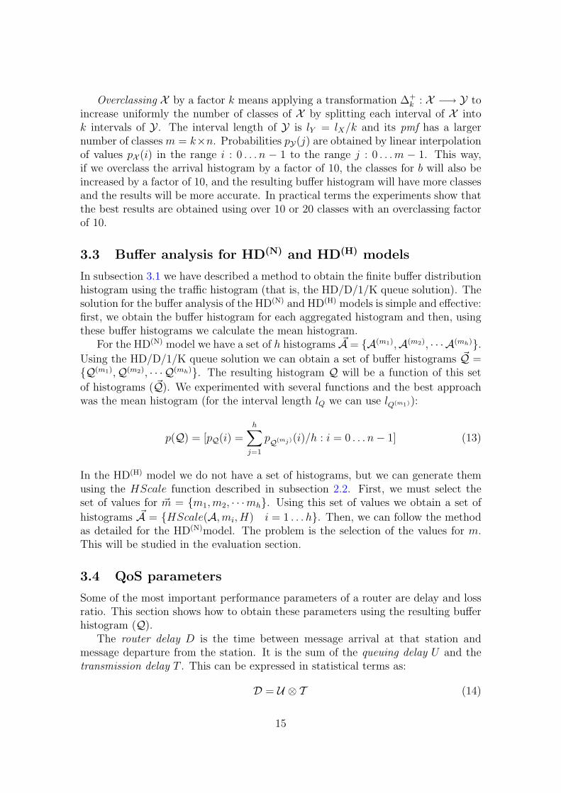
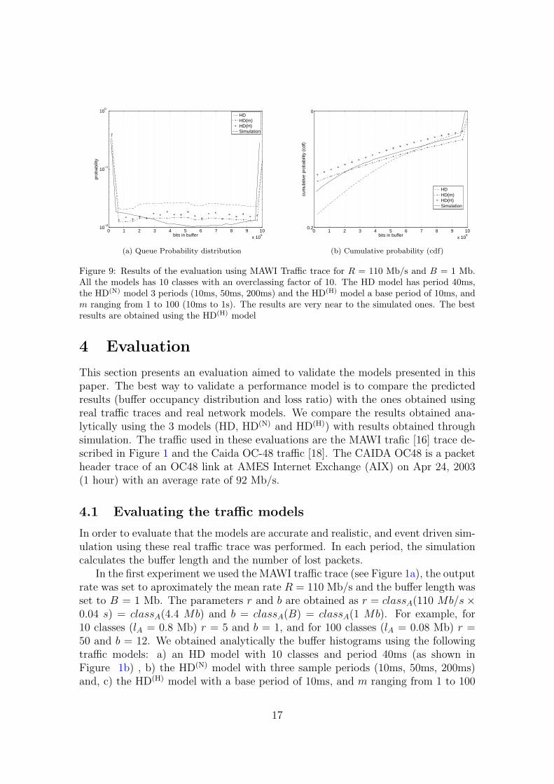
0 1 2 3 4 5 6 7 8 9 10x 10
5
10minus2
10minus1
100
bits in buffer
prob
abili
ty
HDHD(m)HD(H)Simulation
(a) Queue Probability distribution
0 1 2 3 4 5 6 7 8 9 10x 10
5
0
02
bits in buffer
cum
ulat
ive
prob
abili
ty (
cdf)
HDHD(m)HD(H)Simulation
(b) Cumulative probability (cdf)
Figure 9 Results of the evaluation using MAWI Traffic trace for R = 110 Mbs and B = 1 MbAll the models has 10 classes with an overclassing factor of 10 The HD model has period 40msthe HD(N) model 3 periods (10ms 50ms 200ms) and the HD(H) model a base period of 10ms andm ranging from 1 to 100 (10ms to 1s) The results are very near to the simulated ones The bestresults are obtained using the HD(H) model
4 Evaluation
This section presents an evaluation aimed to validate the models presented in thispaper The best way to validate a performance model is to compare the predictedresults (buffer occupancy distribution and loss ratio) with the ones obtained usingreal traffic traces and real network models We compare the results obtained ana-lytically using the 3 models (HD HD(N) and HD(H)) with results obtained throughsimulation The traffic used in these evaluations are the MAWI trafic [16] trace de-scribed in Figure 1 and the Caida OC-48 traffic [18] The CAIDA OC48 is a packetheader trace of an OC48 link at AMES Internet Exchange (AIX) on Apr 24 2003(1 hour) with an average rate of 92 Mbs
41 Evaluating the traffic models
In order to evaluate that the models are accurate and realistic and event driven sim-ulation using these real traffic trace was performed In each period the simulationcalculates the buffer length and the number of lost packets
In the first experiment we used the MAWI traffic trace (see Figure 1a) the outputrate was set to aproximately the mean rate R = 110 Mbs and the buffer length wasset to B = 1 Mb The parameters r and b are obtained as r = classA(110 Mbstimes004 s) = classA(44 Mb) and b = classA(B) = classA(1 Mb) For example for10 classes (lA = 08 Mb) r = 5 and b = 1 and for 100 classes (lA = 008 Mb) r =50 and b = 12 We obtained analytically the buffer histograms using the followingtraffic models a) an HD model with 10 classes and period 40ms (as shown inFigure 1b) b) the HD(N) model with three sample periods (10ms 50ms 200ms)and c) the HD(H) model with a base period of 10ms and m ranging from 1 to 100
17
0 1 2 3 4 5 6 7 8 9 10x 10
5
10minus3
10minus2
10minus1
100
bits in buffer
prob
abili
ty
HDHD(m)HD(H)Simulation
Figure 10 Queue Probability Distribution using the CAIDA OC-48 traffic trace for R = 90 Mbsand B = 1 Mb The HD(N) model is the most accurate
(10ms to 1s) For the histograms we used 10 classes with an overclassing factorof 10 For comparison we obtained the buffer histogram using simulation Thequeue probability distribution is shown in Figure 9a (note that the y-axe is in logscale) We can appreciate better the differences using the cumulative probability(see Figure 9b) The results for the three models are very accurate although bestresults are obtained using the HD(N) model Regarding the loss ratio the simulationprovided a value of 00640109 while the HD model estimated a value of 0041934the HD(N) model 00576173 and 00583313 for the HD(H) model
For the following experiment we used the CAIDA OC-48 traffic The outputrate was set to R = 90 Mbs and the buffer length was set to B = 1 Mb Weobtained analytically the buffer histograms using the same sample periods for thetraffic models of the MAWI experiments The results are in Figure 10 We can seethat the best results are obtained using the HD(m) model Regarding the loss ratiothe simulation provided a value of 00494095 while the HD model estimated a valueof 00344655 the HD(N) model 00436831 and 00426831 for the HD(H) model
Previous experiments used a 1-hour trace for obtaining the histogram producingvery good results The following experiment uses the MAWI 12-hour trace (from800 to 2000 of the Jan 09 2007 traces) The rate was set to R = 120 Mbs and thebuffer length to B = 1 Mb This means using long-term traces instead of short-termtraces Results are still very accurate as shown in Figure 11 Regarding the lossratio the HD model predicted 00146371 HD(N) 00214733 and HD(H) 00202713while the simulation yielded 00275981 In summary there is a little loss of accuracywhen using long-term traces as it could be expected due to information loss in thehistogram representation
Previous experiments were also repeated with different traffic traces (using MAWItraces from a different day and hour and traces from the NLANR repository) out-put rates and buffer lengths Results were very similar to the ones presented here(See [19] for more experiments)
18
0 1 2 3 4 5 6 7 8 9 10x 10
5
10minus3
10minus2
10minus1
100
bits in buffer
prob
abili
ty
HDHD(m)HD(H)Simulation
Figure 11 MAWI long-term traffic queue distribution for R = 120 Mbs and B = 1 Mb Theresults of using a 12-hour trace are still very accurate
42 Accuracy
This subsection is devoted to identify and evaluate factors that may affect the ac-curacy of the results The selection of the number of classes and the sample periodwas based on the results of the following experiments
One of the keys aspect of these traffic models is the selection of the sampleperiods We analyse the relation between the sampling period and accuracy usingthe basic HD model In Figure 12a is the result of obtaining the buffer histogramfor several sample periods (base period = 10ms m = 1 2 5 10 100 ) We cansee that the precision is clearly affected by the sample period The best results areobtained using m = 5 that is a sampling period of 50ms Figure 12b shows thenormalized difference5 between the buffer histograms obtained using the HD trafficand that obtained through simulations varying the sample rate from 10ms to 20sThis figure also shows the loss ratio error that is the relative error between theloss ratio predicted by our model and the ones obtained in the simulation The bestprecision is obtained using periods between 20ms and 100ms
The following experiment analyses the relation between buffer length and lossratio for the HD(N) traffic model Loss ratios are calculated for different output ratesvarying the buffer length between 10 kb and 10 Mb (this corresponds to a maximalqueue delay of less than 01 s) Results are presented in the form of a loss ratiocurve (see Figure 13) The prediction of loss rate using the HD(N) traffic model isvery accurate since it is very close to simulations
Regarding on the number of classes several experiments were done varying thenumber of histogram classes The key question is how many classes are necessary toget a good accuracy In the following experiment the number of classes was variedfrom 6 to 100 and 4 histograms were calculated the first one using the originalhistogram with no overclassing and the other 3 using overclassing factors of 5 10and 20 The normalized difference between these histograms and the one obtained
5the normalized difference of 2 vectors A=[a1 middot middot middot an] and B=[b1 middot middot middot bn] is defined asradic(a1 minus b1) + middot middot middot+ (an minus bn)
19
0 1 2 3 4 5 6 7 8 9 10x 10
5
10minus06
10minus05
10minus04
10minus03
10minus02
10minus01
bits in buffer
cum
ulat
ive
prob
abili
ty (
cdf)
HD(1)HD(2)HD(5)HD(10)HD(100)Simulation
(a)
10minus2
10minus1
100
1010
005
01
015
02
025
03
period (s)
Diff
eren
ce
Histogram differenceLoss ratio error
(b)
Figure 12 Sample Period and precision a) Queue Probability distribution for several sampleperiods (base period = 10ms) We can see the precision of the result depends clearly on the baseperiod b) This graph shows the Normalized difference between the histograms and the loss ratioerror obtained using the HD model and the simulations for sample rate between 10ms and 20sThe best results are obtained for periods between 20ms and 100ms
0 1 2 3 4 5 6 7 8 9 10
x 106
0
002
004
006
008
01
012
buffer
Histogram R=100MbsSimulation R=100MbHistogram R=120MbSimulation R=120MbsHistogram R=150MbsSimulation R=150Mbs
Figure 13 Loss Ratio Curve the loss ratio is obtained for the the HD(N) model and is comparedto the results obtained in the simulation using different output rates (R=100 110 and 120 Mbs)and varying the buffer length The results are very accurate for R=100Mbs For R=120Mbsthere is a loss of precision in some ranges
20
0 20 40 60 80 100
1
05
classes
norm
aliz
ed d
iffer
ence
x1x5x10x20
(a) Normalized difference for R = 110Mbs B = 1Mb
0 20 40 60 80 100009
01
011
012
013
014
015
016
017
classes
cell
loss
rat
io
x1x5x10x20Simulation
(b) Cell loss ratio for R = 100Mbs B = 1Mb
Figure 14 Relation between Number of Classes overclassing and precision the number of classeswas varied from 6 to 100 and 4 histograms were calculated rsquox1rsquo original histogram rsquox5rsquorsquox10rsquo andrsquox20rsquo with overclassing factors of 5 10 and 20 We can see that accuracy is not greatly improvedusing more than 15 classes and better results are obtaining using an overclassing factor of 10
through simulation is shown in Figure 14a The loss ratio is compared with the lossratio of simulations in Figure 14b Results show that the main effect of overclassingis to smooth the results reducing the original peaks It can be also seen that thereis no significant variation using a overclassing factor greater than 10 Regarding onthe number of original classes it can be seen that accuracy is not greatly improvedusing more than 15 of 20 classes For the original histogram accuracy is betterin some cases using more than 60 classes (see Figure 14a) but in some other casesit is worst Therefore in the average case it is better to use overclassing Thefinal conclusion is that the best results are obtained using 10 to 20 classes with anoverclassing factor of 10
43 Long-range dependence implications on the models
In [17] is discussed the impact of the long-range dependence (LRD) on the bufferoccupancy and indicated that LRD does not affect the buffer occupancy when thebusy periods of the system are not large Similar conclusions were obtained in [20]short-term correlation have dominant effect on cell loss ratio More important is tochoose the critical time scale (CTS) that is related with the sample period In [20]the authors considered the buffer behavior at the time-scale beyond the CTS is nosignificantly affected The experiments of this paper showed that the best modelwas HD(N) that is not strictly LRD Therefore the results confirms the results of [20]and [17] Our experiments shows that when selecting correctly the sampling periodthe results are very accurate
Another question is the selection of the model Each model has its pros andcons
bull HD model this model is simple and compact and the results are still veryaccurate It is a good approximation
21
0 1 2 3 4 5 6 7 8 9 10x 10
5
10minus4
10minus3
10minus2
10minus1
100
bits in buffer
prob
abili
ty
HD(m) modelHistogram MD1K methodPacket Simulation
(a)
0 05 1 15 2 25 3 35 4 45 5x 10
6
003
004
005
006
007
008
009
01
011
012
buffer
simulationHD(M) modelMVA
(b)
Figure 15 Comparison with other methods a) Comparison of the buffer histograms obtainedusing our HD(N) model and the MD1K approach by Skelly and Shroff ( [12] for R = 110Mbs B= 1Mb We can see that the MD1K approach collapses when the buffer is large b) Comparison ofthe cell loss ratio obtained using the Maximum Variance Asymptotic (MVA) method versus theHD(N) model results R = 110Ms The graph shows a better precision of the HD(N) model
bull HD(N) it is the more accurate model but it is not so compact We must obtainseveral histograms for several periods so it can be cumbersome
bull HD(H) this model is still compact (we only need one histogram and the Hurstparameter) and the results are very good
44 Comparison with other methods
This section compares the model with previously published methods for analyzingbuffer length and loss ratio To simplify we only compare the results of the HD(N)
model Regarding the calculation of the buffer length the best known approach isthe method introduced by Skelly and Shroff (known as the Histogram Model [12]or the Generalized Histogram Model [13] and used with few modifications in [21]and [22]) This approximation is based on resolving an MD1N queue for eacharrival rate of the histogram We implemented this method and compared theobtained buffer length histogram with the one obtained using the HD(N) modelFigure 15a shows that the differences between the HBSP model and the MD1Nmethod are large The results using the MD1N are imprecise The problemswith the MD1N is that the buffer curve collapses when the buffer size if highThe results presented in [12] used very low buffer lengths (about 50 cells) so theresults were more accurate Nevertheless when larger buffer (about 500) the buffercurve begins to collapse
Regarding the loss ratio most of the papers deal with the tail probability (oroverflow probability) P (Q gt t) rather than the loss probability In this paperwe compare the HBSP method versus the Maximum Variance Asymptotic (MVA)approximation for loss detailed in [11] In Figure 15b we can see the loss probability
22
Ingress
node1
Egress
node 2 node 3
node 6
node 5
node 4
node 7
Channel
0
3
0 1 2 3 4
0
3
0 1 2 3 4
0
3
0 1 2 3 4
0
7
0 1 2 3 4
0
3
0 1 2 3 4
0
4
0 1 2 3 4
0
3
0 1 2 3 4
0
4
0 1 2 3 4
0
4
0 1 2 3 4
Figure 16 Sample network with the load histograms of the nodes This can be seen as a visualmonitorization of the network load With this information we can obtain the loss ratio the end-to-end delay distribution for a given path
depending on the buffer size The graph shows that the HD(N) cell loss curve is moreprecise than the MVA curve
5 Applications of the model
There is a wide spectrum of applications of the HBSP model We can obtain thetraffic QoS parameters as loss ratio or node delay using the HBSP model Usingthe router delay of the nodes we can obtain the network delay pmf DN This pmfis obtained as the sum (convolution) of the node pmfs that a packet traverses
DN =otimesiisinpath
Di (19)
For example using Figure 16 we can obtain the end-to-end delay distribution forthe path marked with blue This pmf is very useful because we can obtain the meandelay or for example the probability that a packet is delayed more than a certainvalue For example if we transmit video or audio the delay histogram can be usefulin the end nodes to adapt their transmissions rates or to configure the buffer in thereception nodes This information can be used for admission control as well
Another important application is for traffic provisioning and network configura-tion Optimal provisioning of network resources is crucial for reducing the servicecost of network transmission This is the goal of Traffic Engineering the designprovisioning performance evaluation and tuning of operational networks The fun-damental problem with provisioning is to have methods and tools to decide the net-work resource reservation for a given Quality of Service requirements [23] Thereforethe HBSP method can be very useful for Traffic Engineering The HBSP methodallows to obtain the load histogram of the nodes of a network These histograms canbe used to configure the network For example if we have a network like the one
23
presented in Figure 16 we can see that node 4 is highly loaded and we can decide toincrease its resource or to change some route in order to reduce the load in node 4
It also allows to evaluate parameters like the loss ratio (for a given buffer andoutput ratio) the node delay the bufferoutput ratio needed for a required loss etcOne important decision that must be taken is the time-scale of the provisioning Themeasured traffic can be a long-term trace (daily or weekly traces) or a short-termtrace (hourly traces) This depends on the network capability to support dynamicalvariation in the reservation of the channel resources (for example an hour) (see [24])
A great advantage of the HBSP model is the easy implementation of the his-tograms Is very easy to capture and store a load histogram with few classes (about10) in a network node
6 Conclusions
This paper introduces three traffic models and a performance model to obtain thefinite buffer occupancy distribution The performace model is based on a stochasticprocess working with histograms for resolving the HDD1K queue The resultof this stochastic process is a histogram of the buffer distribution This bufferdistribution has an easy solution for the infinite buffer case but it seems to havea complicated solution for the finite buffer case [17] For this reason most of thepapers obtains the tail probability P (Q gt t) using an infinite buffer model andapproximate the cell loss using this tail probability The model presented in thispaper is a solution of the finite buffer case From the buffer histogram and thearrival histogram it is easy to obtain the cell loss ratio
Three models are described in this paper The first model (HD) is a basichistogram model that is compact and short-range dependent The second one (theHD(N) model) is based on obtaining several histograms using different time scalesThe third one (the HD(H) model) is based on the Hurst parameter and it is long-range dependent Experiments were performed using several real-traffic traces Thebest results are obtaining using the HD(N) model although it can be cumbersomeSo the best approach is the HD(H) model that is compact and it is very precise
There is a wide spectrum of applications of this model We can obtain the trafficQoS parameters as loss ratio or node delay The delay histogram is very usefulbecause we can obtain the mean delay or for example the probability that a packetis delayed more than a certain value For example if we transmit video or audio thedelay histogram can be useful in the end nodes to adapt their transmissions ratesor to configure the buffer in the reception nodes This information can be used foradmission control as well Another important application is for traffic provisioningand network configuration Optimal provisioning of network resources is crucial forreducing the service cost of network transmission
24
7 Acknowledgments
This work was developed under grants of the Generalitat Valenciana (GV2007192)and the Spanish Government (CICYT TIN2005-08665-C03-03)
References
[1] Ronald G Addie Moshe Zukerman and Timothy D Neame Broadband trafficmodeling Simple solutions to hard problems IEEE Communications Magazinepages 88ndash95 August 1998
[2] Will E Leland Murad S Taqqu Walter Willinger and Daniel V Wilson On theself-similar nature of ethernet traffic (extended version) IEEEACM Trans Netw2(1)1ndash15 1994
[3] Vern Paxson and Sally Floyd Wide area traffic the failure of poisson modelingIEEEACM Trans Netw 3(3)226ndash244 1995
[4] Jin Cao William S Cleveland Dong Lin and Don X Sun Nonlinear Estimationand Classification chapter Internet Traffic Tends Toward Poisson and Independentas the Load Increases Springer 2002
[5] E Casilari JM Cano-Garcia FJ Gonzalez-Canete and F Sandoval Modellingof individual and aggregate web traffic In IEEE International Conference on HighSpeed Networks and Multimedia Communications HSNMC pages 84ndash95 2004
[6] P Abry R Baraniuk P Flandrin R Riedi and D Veitch Multiscale nature ofnetwork traffic IEEE Signal Processing Magazine 19(3)28ndash46 2002
[7] David L Jagerman Benjamin Melamed and Walter Willinger Stochastic modelingof traffic processes pages 271ndash320 1997
[8] David M Lucantoni The BMAPG1 queue A tutorial In Performance Evaluationof Computer and Communication Systems Joint Tutorial Papers of Performance rsquo93and Sigmetrics rsquo93 pages 330ndash358 London UK 1993 Springer-Verlag
[9] Alexander Klemm Christoph Lindemann and Marco Lohmann Modeling ip trafficusing the batch markovian arrival process Performance Evaluation 54149ndash173 2003
[10] On Hassida Yoshitaka Takahashi and Shinsuke Shimogawa Multiscale nature ofnetwork traffic Switched Batch Bernoulli Process (SBBP) and the Discrete-timeSBBPG1 queue with Application to Statistical Multiplexer Performance 9(3)394ndash401 1991
[11] Han S Kim and Ness B Shroff On the asymptotic relationship between the overflowprobability and the loss ratio IEEEACM Trans Netw 9(6)755ndash768 2001
[12] P Skelly M Schwartz and S Dixit A histogram-based model for video trafficbehavior in an ATM multiplexer IEEEACM Transactions on Networking 1(4)446ndash459 August 1993
25
[13] Ness B Shroff and Mischa Schwartz Video modeling withing networks using deter-ministic smoothing at the source In IEEE Infocom pages 342ndash349 1994
[14] J Luthi S Majumdar and G Haring Mean value analysis for computer systemswith variabilities in workload In IPDS rsquo96 Proceedings of the 2nd InternationalComputer Performance and Dependability Symposium page 32 Washington DCUSA 1996 IEEE Computer Society
[15] Moshe Zukerman Timothy D Neame and Ronald G Addie Internet traffic modelingand future technology implications In IEEE Infocom 2003
[16] K Cho and et al Traffic data repository at the wide project In USENIX 2000FREENIX Track 6 2000
[17] Daniel P Heyman and T V Lakshman What are the implications of long-rangedependence for VBR-video traffic engineering IEEEACM Trans Netw 4(3)301ndash317 1996
[18] DatCat Caida oc48 traces 2003-04-24 download in httpimdcdatcatorg
[19] E Hernandez and JVila A stochastic analysis of network traffic based on histogramworkload modelling Technical Report UPV-DISCA-06-09 September 2006 Down-load in httpwwwdiscaupvesenherorpdfTR_DISCA_06_09pdf
[20] Bong K Ryu and Anwar Elwalid The importance of long-range dependence of VBRvideo traffic in ATM traffic engineering myths and realities In SIGCOMM rsquo96pages 3ndash14 New York NY USA 1996 ACM Press
[21] Ness B Shroff and M Schwartz Improved loss calculations at an ATM multiplexerIEEEACM Transactions on Networking 6(4)411ndash21 August 1998
[22] Seok-Kyu Kweon and Kang G Shin Real-time transport of MPEG video with astatistically guaranteed loss ratio in ATM networks IEEE Transactions In Paralleland Distributed Computing 12(4)387ndash403 April 2001
[23] D Awduche and et al Overview and principles of internet traffic engineering RFC3272 May 2002
[24] Enrique Hernandez-Orallo Joan Vila-Carbo Sergio Saez-Barona and Silvia Terrasa-Barrena Provisioning expedited forwarding diffserv channels using multimedia ag-gregates In Euromicro 2004 9 2004
A Method for scaling and histogram
This appendix describes how to obtain the m-aggregated histogram A with a vari-ance according to the scaling function m2Hminus2 The function that obtains this newhistogram will be named HScale That is A = HScale(AmH) generates a newhistogram A with variance m2Hminus2 middotV ar(A) pmf p(A) = [pA(i) i = 0 nminus 1] andinterval length lA middotm
26
As the variance of A must be reduced we are going to shrink the histogramFor example if we have the histogram p(A) = [02 06 02] that has mean 1 andvariance 04 and we want to decrease its variance to 03 the new histogram will be[015 07 015]
The goal is to shrink the histogram reducing the values at the edges and ac-cumulating this reduction for the classes in the mean Assume that the histogramhas n classes and the classes in the mean are h = bE(A)c and h + 1 We startin the left edge The probability of class 0 (p0 = pA(0)) is reduced by a factor c(05 lt c lt 1) That is p0 = pA(0) = c middot p0 This reduction ((1 minus c) middot p0) is accu-mulated to class 1 that is also reduced by c p1 = c middot p1 + (1 minus c) middot p0 For classhminus 1 we have phminus1 = c middot phminus1 + (1minus c) middot phminus2 For the classes in the mean we mustcalculate another reducing factor cprime The reason is to reduce these classes accordingto the mean For example if the mean is very near the class h we must reduce theclass h + 1 accordingly On the other hand if the mean is near to class h + 1 wemust reduce the class h This factor is obtained as cprime = 05minus (hminus E(A)) Assumecprime gt 0 (mean near class h) then we have ph = ph + (1 minus c) middot phminus1 + cprime middot ph+1 andph+1 = (1minuscprime) middotph+1 +(1minusc) middotph+2 For cprime lt 0 is similar The right side is equivalentto the left So we have
p0 = c middot p0 = p0 middot cp1 = c middot p1 + (1minus c) middot p0 = p0 + (p1 minus p0) middot c
phminus1 = c middot phminus1 + (1minus c) middot phminus2 = phminus2 + (phminus1 minus phminus2) middot cph = ph + (1minus c) middot phminus1 + cprime middot ph+1 = ph + phminus1 + cprime middot ph+1 + minusphminus1 middot cph+1 = (1minus cprime) middot ph+1 + (1minus c) middot ph+2 = (1minus cprime) middot ph+1 + ph+2 + minusph+2 middot cph+2 = c middot ph+2 + (1minus c) middot ph+3 = ph+3 + (ph+2 minus ph+3) middot c
pnminus1 = c middot pnminus1 = pnminus1 middot c(20)
It is easy to see thatsumnminus1
0 pi = 1The goal of the following method is to transform a histogram A to a scaled
histogram A with variance v = m2Hminus2 middot V ar(A) We have
V ar(A) =nminus1sum
0
(iminus E[A])2︸ ︷︷ ︸di
middotpi =nminus1sum
0
di middot pi = v (21)
Then we multiply all the terms in equation 20 by di and summing all the probabil-ities and grouping terms we have
sumnminus10 di middot pi = Sc middot c+ S = v (the SA coefficient is
the sum of all the coefficients of the c variable and SB is the sum of the coefficientswithout variable) Then the reducing factor c is obtained as
c =v minus SSc
(22)
27
For obtaining the coefficients we must obtain the values of di We need to estimatethe value of E[A] The mean of the original histogram (E[A]) is a good estimatorUsing this mean we obtain the sum of the coefficients and resolve equation 22 Withthis factor c we apply equations 20 for obtaining the distribution of A Normallythe variance of A will not be exactly v because we are estimating the mean as E[A]So we can repeat the calculations using the mean of the calculated histogram E[A]Practically in 2 or 3 iterations we obtain the desired histogram with the requiredvariance If the result of c is not in the range 05 lt c lt 1 this mean that the desiredvariance can not be obtained in one step So we apply a factor of 05 to obtain anew histogram that is shrunk by a factor of 05 and using this new histogram wecan obtain a new factor c until the factor is greater than 05
The algorithm of the HScale function is outlined in Figure 17 In the algorithmwe have 2 functions The function SumCoef obtains the sum of the coefficients SAand SB for a given mean and the function Getpmf calculate the pmf according toequation 20
As an example of how the function works we will use the MAWI histogram ofFigure 1b p(A) = [00003 00002 00021 00641 02663 03228 02345 0098000110 00005] that has a base period of 004ms variance 1282 and an intervallength of lA = 008Mb For m = 10 and H = 085 the result is p(A) = [0000100002 00010 00289 01478 06580 01105 00481 00050 00002] with an inter-val length of 8Mb The variance is 06334 according to v = var(A) middotm2Hminus2
B Buffer analysis as a DTMC
In this appendix we show that the stochastic process Qk is a Discrete-Time MarkovChain (DTMC) Additionally we can easily obtain the transition probability matrixP Using this probability matrix we can obtain the values for Qk The problem ofusing DTMC it that is not easy to obtain an analytical solution for the steady state(that is when k rarrinfin)
A Discrete-Time Markov Chain is a stochastic process whose probabilities distri-butions in state j only depends on the previous state i and not on how the processarrived to state i It is easy to proof that Qk is a DTMC The probability that thebuffer in period k takes the value j can be expressed using the buffer probabilitiesof period k minus 1 as follows
P [Qk = j] =sumi
P [Qkminus1 = i] middot P [Qk = j|Qkminus1 = i] (23)
The term pij(k minus 1 k) = P [Qk = j|Qkminus1 = i] denotes the probability that theprocess makes a transition from state i at period k minus 1 to state j at period k Thisprobability is obtained from the arrival load A and given that A is the same in allthe periods then the pij(k minus 1 k) does not depend on the period k Therefore wecan represent pij(k minus 1 k) as pij and Equation 24 is reduced to
P [Qk = j] =sumi
P [Qkminus1 = i] middot pij (24)
28
Algorithm A = HScale(A m H)inputA rsquoOriginal histogramm rsquoAggregationH rsquoHurst parameteroutputA rsquoHistogram for the m-aggregation
1 begin3 v = V ar(A) middotm(2minus2H)Ac = A4 while true5 mean = E[Ac]6 do7 [S Sc] = SumCoef(Ac mean)8 c = (v minus S)Sc9 Af = Getpmf(Ac c mean) rsquoCalculate the pmf for c10 mean = E[Af ] rsquoRepeat with a new mean11 while (05 lt c lt 1) and (|V ar(Af )minus v| lt ε)12 if 05 lt c lt 113 A = Af rsquoThe histogram has Var=v14 return15 else16 mean = E[Ac]17 Ac = Getpmf(Ac 05 mean) rsquoScale the histogram by 0518 end if19 end while20 end
Figure 17 The fv algorithm
29
pij is known as the one-step transition probability From this we can obtain thetransition probability matrix
P = [pij] =
p00 p01 p02 middot middot middotp10 p11 p12 middot middot middot
(25)
The components of this matrix are easy to obtain using the definition of the stochas-tic process Qk That is for obtaining the i-row of P we apply one iteration of thestochastic process using an initial load of one unit in j For example the first rowis obtained as Φb
r([1 0 0 0 ] A) Using the matrix P we can obtain the pmf ofQk as
Qk = Q1Pk (26)
Nevertheless determining the asymptotic behavior (that is the steady state) posesproblems This implies obtaining the steady-state probability vector v as
v = vP vj ge 0sumj
vj = 1 (27)
This matrix has a finite size of (b+ 1)times (b+ 1) Nevertheless numerically resolvingEquation 27 is not easy even for a little matrix Therefore we must use iterativemethods as the power method or something similar
Using the example of subsection 31 p(A) =[00003 00002 00021 0064102663 03228 02345 00980 00110 00005] with r=5 and b=4 we obtain thefollowing matrix
P =
06558 02345 00980 00110 0000503330 03228 02345 00980 0011500667 02663 03228 02345 0109500026 00641 02663 03228 0344000005 00021 00641 02663 06668
(28)
We can obtain the second iteration state as Q2 = Q1P = [05147 02563 0153900569 00179] The steady state probability vector is v = [01912 01585 0185201960 02691] This is the pmf of Q (p(Q))
30
- 1 Introduction
- 2 Traffic Workload Models
-
- 21 Basic Histogram Workload Model
- 22 Second-order Statistics models
-
- 3 Network Peformance Model
-
- 31 Basic Finite-Buffer Occupancy Analysis
- 32 Histogram classes and precision
- 33 Buffer analysis for HD(N) and HD(H) models
- 34 QoS parameters
-
- 4 Evaluation
-
- 41 Evaluating the traffic models
- 42 Accuracy
- 43 Long-range dependence implications on the models
- 44 Comparison with other methods
-
- 5 Applications of the model
- 6 Conclusions
- 7 Acknowledgments
- A Method for scaling and histogram
- B Buffer analysis as a DTMC
-

0 1 2 3 4 5 6 7 8 9 10x 10
5
10minus3
10minus2
10minus1
100
bits in buffer
prob
abili
ty
HDHD(m)HD(H)Simulation
Figure 11 MAWI long-term traffic queue distribution for R = 120 Mbs and B = 1 Mb Theresults of using a 12-hour trace are still very accurate
42 Accuracy
This subsection is devoted to identify and evaluate factors that may affect the ac-curacy of the results The selection of the number of classes and the sample periodwas based on the results of the following experiments
One of the keys aspect of these traffic models is the selection of the sampleperiods We analyse the relation between the sampling period and accuracy usingthe basic HD model In Figure 12a is the result of obtaining the buffer histogramfor several sample periods (base period = 10ms m = 1 2 5 10 100 ) We cansee that the precision is clearly affected by the sample period The best results areobtained using m = 5 that is a sampling period of 50ms Figure 12b shows thenormalized difference5 between the buffer histograms obtained using the HD trafficand that obtained through simulations varying the sample rate from 10ms to 20sThis figure also shows the loss ratio error that is the relative error between theloss ratio predicted by our model and the ones obtained in the simulation The bestprecision is obtained using periods between 20ms and 100ms
The following experiment analyses the relation between buffer length and lossratio for the HD(N) traffic model Loss ratios are calculated for different output ratesvarying the buffer length between 10 kb and 10 Mb (this corresponds to a maximalqueue delay of less than 01 s) Results are presented in the form of a loss ratiocurve (see Figure 13) The prediction of loss rate using the HD(N) traffic model isvery accurate since it is very close to simulations
Regarding on the number of classes several experiments were done varying thenumber of histogram classes The key question is how many classes are necessary toget a good accuracy In the following experiment the number of classes was variedfrom 6 to 100 and 4 histograms were calculated the first one using the originalhistogram with no overclassing and the other 3 using overclassing factors of 5 10and 20 The normalized difference between these histograms and the one obtained
5the normalized difference of 2 vectors A=[a1 middot middot middot an] and B=[b1 middot middot middot bn] is defined asradic(a1 minus b1) + middot middot middot+ (an minus bn)
19
0 1 2 3 4 5 6 7 8 9 10x 10
5
10minus06
10minus05
10minus04
10minus03
10minus02
10minus01
bits in buffer
cum
ulat
ive
prob
abili
ty (
cdf)
HD(1)HD(2)HD(5)HD(10)HD(100)Simulation
(a)
10minus2
10minus1
100
1010
005
01
015
02
025
03
period (s)
Diff
eren
ce
Histogram differenceLoss ratio error
(b)
Figure 12 Sample Period and precision a) Queue Probability distribution for several sampleperiods (base period = 10ms) We can see the precision of the result depends clearly on the baseperiod b) This graph shows the Normalized difference between the histograms and the loss ratioerror obtained using the HD model and the simulations for sample rate between 10ms and 20sThe best results are obtained for periods between 20ms and 100ms
0 1 2 3 4 5 6 7 8 9 10
x 106
0
002
004
006
008
01
012
buffer
Histogram R=100MbsSimulation R=100MbHistogram R=120MbSimulation R=120MbsHistogram R=150MbsSimulation R=150Mbs
Figure 13 Loss Ratio Curve the loss ratio is obtained for the the HD(N) model and is comparedto the results obtained in the simulation using different output rates (R=100 110 and 120 Mbs)and varying the buffer length The results are very accurate for R=100Mbs For R=120Mbsthere is a loss of precision in some ranges
20
0 20 40 60 80 100
1
05
classes
norm
aliz
ed d
iffer
ence
x1x5x10x20
(a) Normalized difference for R = 110Mbs B = 1Mb
0 20 40 60 80 100009
01
011
012
013
014
015
016
017
classes
cell
loss
rat
io
x1x5x10x20Simulation
(b) Cell loss ratio for R = 100Mbs B = 1Mb
Figure 14 Relation between Number of Classes overclassing and precision the number of classeswas varied from 6 to 100 and 4 histograms were calculated rsquox1rsquo original histogram rsquox5rsquorsquox10rsquo andrsquox20rsquo with overclassing factors of 5 10 and 20 We can see that accuracy is not greatly improvedusing more than 15 classes and better results are obtaining using an overclassing factor of 10
through simulation is shown in Figure 14a The loss ratio is compared with the lossratio of simulations in Figure 14b Results show that the main effect of overclassingis to smooth the results reducing the original peaks It can be also seen that thereis no significant variation using a overclassing factor greater than 10 Regarding onthe number of original classes it can be seen that accuracy is not greatly improvedusing more than 15 of 20 classes For the original histogram accuracy is betterin some cases using more than 60 classes (see Figure 14a) but in some other casesit is worst Therefore in the average case it is better to use overclassing Thefinal conclusion is that the best results are obtained using 10 to 20 classes with anoverclassing factor of 10
43 Long-range dependence implications on the models
In [17] is discussed the impact of the long-range dependence (LRD) on the bufferoccupancy and indicated that LRD does not affect the buffer occupancy when thebusy periods of the system are not large Similar conclusions were obtained in [20]short-term correlation have dominant effect on cell loss ratio More important is tochoose the critical time scale (CTS) that is related with the sample period In [20]the authors considered the buffer behavior at the time-scale beyond the CTS is nosignificantly affected The experiments of this paper showed that the best modelwas HD(N) that is not strictly LRD Therefore the results confirms the results of [20]and [17] Our experiments shows that when selecting correctly the sampling periodthe results are very accurate
Another question is the selection of the model Each model has its pros andcons
bull HD model this model is simple and compact and the results are still veryaccurate It is a good approximation
21
0 1 2 3 4 5 6 7 8 9 10x 10
5
10minus4
10minus3
10minus2
10minus1
100
bits in buffer
prob
abili
ty
HD(m) modelHistogram MD1K methodPacket Simulation
(a)
0 05 1 15 2 25 3 35 4 45 5x 10
6
003
004
005
006
007
008
009
01
011
012
buffer
simulationHD(M) modelMVA
(b)
Figure 15 Comparison with other methods a) Comparison of the buffer histograms obtainedusing our HD(N) model and the MD1K approach by Skelly and Shroff ( [12] for R = 110Mbs B= 1Mb We can see that the MD1K approach collapses when the buffer is large b) Comparison ofthe cell loss ratio obtained using the Maximum Variance Asymptotic (MVA) method versus theHD(N) model results R = 110Ms The graph shows a better precision of the HD(N) model
bull HD(N) it is the more accurate model but it is not so compact We must obtainseveral histograms for several periods so it can be cumbersome
bull HD(H) this model is still compact (we only need one histogram and the Hurstparameter) and the results are very good
44 Comparison with other methods
This section compares the model with previously published methods for analyzingbuffer length and loss ratio To simplify we only compare the results of the HD(N)
model Regarding the calculation of the buffer length the best known approach isthe method introduced by Skelly and Shroff (known as the Histogram Model [12]or the Generalized Histogram Model [13] and used with few modifications in [21]and [22]) This approximation is based on resolving an MD1N queue for eacharrival rate of the histogram We implemented this method and compared theobtained buffer length histogram with the one obtained using the HD(N) modelFigure 15a shows that the differences between the HBSP model and the MD1Nmethod are large The results using the MD1N are imprecise The problemswith the MD1N is that the buffer curve collapses when the buffer size if highThe results presented in [12] used very low buffer lengths (about 50 cells) so theresults were more accurate Nevertheless when larger buffer (about 500) the buffercurve begins to collapse
Regarding the loss ratio most of the papers deal with the tail probability (oroverflow probability) P (Q gt t) rather than the loss probability In this paperwe compare the HBSP method versus the Maximum Variance Asymptotic (MVA)approximation for loss detailed in [11] In Figure 15b we can see the loss probability
22
Ingress
node1
Egress
node 2 node 3
node 6
node 5
node 4
node 7
Channel
0
3
0 1 2 3 4
0
3
0 1 2 3 4
0
3
0 1 2 3 4
0
7
0 1 2 3 4
0
3
0 1 2 3 4
0
4
0 1 2 3 4
0
3
0 1 2 3 4
0
4
0 1 2 3 4
0
4
0 1 2 3 4
Figure 16 Sample network with the load histograms of the nodes This can be seen as a visualmonitorization of the network load With this information we can obtain the loss ratio the end-to-end delay distribution for a given path
depending on the buffer size The graph shows that the HD(N) cell loss curve is moreprecise than the MVA curve
5 Applications of the model
There is a wide spectrum of applications of the HBSP model We can obtain thetraffic QoS parameters as loss ratio or node delay using the HBSP model Usingthe router delay of the nodes we can obtain the network delay pmf DN This pmfis obtained as the sum (convolution) of the node pmfs that a packet traverses
DN =otimesiisinpath
Di (19)
For example using Figure 16 we can obtain the end-to-end delay distribution forthe path marked with blue This pmf is very useful because we can obtain the meandelay or for example the probability that a packet is delayed more than a certainvalue For example if we transmit video or audio the delay histogram can be usefulin the end nodes to adapt their transmissions rates or to configure the buffer in thereception nodes This information can be used for admission control as well
Another important application is for traffic provisioning and network configura-tion Optimal provisioning of network resources is crucial for reducing the servicecost of network transmission This is the goal of Traffic Engineering the designprovisioning performance evaluation and tuning of operational networks The fun-damental problem with provisioning is to have methods and tools to decide the net-work resource reservation for a given Quality of Service requirements [23] Thereforethe HBSP method can be very useful for Traffic Engineering The HBSP methodallows to obtain the load histogram of the nodes of a network These histograms canbe used to configure the network For example if we have a network like the one
23
presented in Figure 16 we can see that node 4 is highly loaded and we can decide toincrease its resource or to change some route in order to reduce the load in node 4
It also allows to evaluate parameters like the loss ratio (for a given buffer andoutput ratio) the node delay the bufferoutput ratio needed for a required loss etcOne important decision that must be taken is the time-scale of the provisioning Themeasured traffic can be a long-term trace (daily or weekly traces) or a short-termtrace (hourly traces) This depends on the network capability to support dynamicalvariation in the reservation of the channel resources (for example an hour) (see [24])
A great advantage of the HBSP model is the easy implementation of the his-tograms Is very easy to capture and store a load histogram with few classes (about10) in a network node
6 Conclusions
This paper introduces three traffic models and a performance model to obtain thefinite buffer occupancy distribution The performace model is based on a stochasticprocess working with histograms for resolving the HDD1K queue The resultof this stochastic process is a histogram of the buffer distribution This bufferdistribution has an easy solution for the infinite buffer case but it seems to havea complicated solution for the finite buffer case [17] For this reason most of thepapers obtains the tail probability P (Q gt t) using an infinite buffer model andapproximate the cell loss using this tail probability The model presented in thispaper is a solution of the finite buffer case From the buffer histogram and thearrival histogram it is easy to obtain the cell loss ratio
Three models are described in this paper The first model (HD) is a basichistogram model that is compact and short-range dependent The second one (theHD(N) model) is based on obtaining several histograms using different time scalesThe third one (the HD(H) model) is based on the Hurst parameter and it is long-range dependent Experiments were performed using several real-traffic traces Thebest results are obtaining using the HD(N) model although it can be cumbersomeSo the best approach is the HD(H) model that is compact and it is very precise
There is a wide spectrum of applications of this model We can obtain the trafficQoS parameters as loss ratio or node delay The delay histogram is very usefulbecause we can obtain the mean delay or for example the probability that a packetis delayed more than a certain value For example if we transmit video or audio thedelay histogram can be useful in the end nodes to adapt their transmissions ratesor to configure the buffer in the reception nodes This information can be used foradmission control as well Another important application is for traffic provisioningand network configuration Optimal provisioning of network resources is crucial forreducing the service cost of network transmission
24
7 Acknowledgments
This work was developed under grants of the Generalitat Valenciana (GV2007192)and the Spanish Government (CICYT TIN2005-08665-C03-03)
References
[1] Ronald G Addie Moshe Zukerman and Timothy D Neame Broadband trafficmodeling Simple solutions to hard problems IEEE Communications Magazinepages 88ndash95 August 1998
[2] Will E Leland Murad S Taqqu Walter Willinger and Daniel V Wilson On theself-similar nature of ethernet traffic (extended version) IEEEACM Trans Netw2(1)1ndash15 1994
[3] Vern Paxson and Sally Floyd Wide area traffic the failure of poisson modelingIEEEACM Trans Netw 3(3)226ndash244 1995
[4] Jin Cao William S Cleveland Dong Lin and Don X Sun Nonlinear Estimationand Classification chapter Internet Traffic Tends Toward Poisson and Independentas the Load Increases Springer 2002
[5] E Casilari JM Cano-Garcia FJ Gonzalez-Canete and F Sandoval Modellingof individual and aggregate web traffic In IEEE International Conference on HighSpeed Networks and Multimedia Communications HSNMC pages 84ndash95 2004
[6] P Abry R Baraniuk P Flandrin R Riedi and D Veitch Multiscale nature ofnetwork traffic IEEE Signal Processing Magazine 19(3)28ndash46 2002
[7] David L Jagerman Benjamin Melamed and Walter Willinger Stochastic modelingof traffic processes pages 271ndash320 1997
[8] David M Lucantoni The BMAPG1 queue A tutorial In Performance Evaluationof Computer and Communication Systems Joint Tutorial Papers of Performance rsquo93and Sigmetrics rsquo93 pages 330ndash358 London UK 1993 Springer-Verlag
[9] Alexander Klemm Christoph Lindemann and Marco Lohmann Modeling ip trafficusing the batch markovian arrival process Performance Evaluation 54149ndash173 2003
[10] On Hassida Yoshitaka Takahashi and Shinsuke Shimogawa Multiscale nature ofnetwork traffic Switched Batch Bernoulli Process (SBBP) and the Discrete-timeSBBPG1 queue with Application to Statistical Multiplexer Performance 9(3)394ndash401 1991
[11] Han S Kim and Ness B Shroff On the asymptotic relationship between the overflowprobability and the loss ratio IEEEACM Trans Netw 9(6)755ndash768 2001
[12] P Skelly M Schwartz and S Dixit A histogram-based model for video trafficbehavior in an ATM multiplexer IEEEACM Transactions on Networking 1(4)446ndash459 August 1993
25
[13] Ness B Shroff and Mischa Schwartz Video modeling withing networks using deter-ministic smoothing at the source In IEEE Infocom pages 342ndash349 1994
[14] J Luthi S Majumdar and G Haring Mean value analysis for computer systemswith variabilities in workload In IPDS rsquo96 Proceedings of the 2nd InternationalComputer Performance and Dependability Symposium page 32 Washington DCUSA 1996 IEEE Computer Society
[15] Moshe Zukerman Timothy D Neame and Ronald G Addie Internet traffic modelingand future technology implications In IEEE Infocom 2003
[16] K Cho and et al Traffic data repository at the wide project In USENIX 2000FREENIX Track 6 2000
[17] Daniel P Heyman and T V Lakshman What are the implications of long-rangedependence for VBR-video traffic engineering IEEEACM Trans Netw 4(3)301ndash317 1996
[18] DatCat Caida oc48 traces 2003-04-24 download in httpimdcdatcatorg
[19] E Hernandez and JVila A stochastic analysis of network traffic based on histogramworkload modelling Technical Report UPV-DISCA-06-09 September 2006 Down-load in httpwwwdiscaupvesenherorpdfTR_DISCA_06_09pdf
[20] Bong K Ryu and Anwar Elwalid The importance of long-range dependence of VBRvideo traffic in ATM traffic engineering myths and realities In SIGCOMM rsquo96pages 3ndash14 New York NY USA 1996 ACM Press
[21] Ness B Shroff and M Schwartz Improved loss calculations at an ATM multiplexerIEEEACM Transactions on Networking 6(4)411ndash21 August 1998
[22] Seok-Kyu Kweon and Kang G Shin Real-time transport of MPEG video with astatistically guaranteed loss ratio in ATM networks IEEE Transactions In Paralleland Distributed Computing 12(4)387ndash403 April 2001
[23] D Awduche and et al Overview and principles of internet traffic engineering RFC3272 May 2002
[24] Enrique Hernandez-Orallo Joan Vila-Carbo Sergio Saez-Barona and Silvia Terrasa-Barrena Provisioning expedited forwarding diffserv channels using multimedia ag-gregates In Euromicro 2004 9 2004
A Method for scaling and histogram
This appendix describes how to obtain the m-aggregated histogram A with a vari-ance according to the scaling function m2Hminus2 The function that obtains this newhistogram will be named HScale That is A = HScale(AmH) generates a newhistogram A with variance m2Hminus2 middotV ar(A) pmf p(A) = [pA(i) i = 0 nminus 1] andinterval length lA middotm
26
As the variance of A must be reduced we are going to shrink the histogramFor example if we have the histogram p(A) = [02 06 02] that has mean 1 andvariance 04 and we want to decrease its variance to 03 the new histogram will be[015 07 015]
The goal is to shrink the histogram reducing the values at the edges and ac-cumulating this reduction for the classes in the mean Assume that the histogramhas n classes and the classes in the mean are h = bE(A)c and h + 1 We startin the left edge The probability of class 0 (p0 = pA(0)) is reduced by a factor c(05 lt c lt 1) That is p0 = pA(0) = c middot p0 This reduction ((1 minus c) middot p0) is accu-mulated to class 1 that is also reduced by c p1 = c middot p1 + (1 minus c) middot p0 For classhminus 1 we have phminus1 = c middot phminus1 + (1minus c) middot phminus2 For the classes in the mean we mustcalculate another reducing factor cprime The reason is to reduce these classes accordingto the mean For example if the mean is very near the class h we must reduce theclass h + 1 accordingly On the other hand if the mean is near to class h + 1 wemust reduce the class h This factor is obtained as cprime = 05minus (hminus E(A)) Assumecprime gt 0 (mean near class h) then we have ph = ph + (1 minus c) middot phminus1 + cprime middot ph+1 andph+1 = (1minuscprime) middotph+1 +(1minusc) middotph+2 For cprime lt 0 is similar The right side is equivalentto the left So we have
p0 = c middot p0 = p0 middot cp1 = c middot p1 + (1minus c) middot p0 = p0 + (p1 minus p0) middot c
phminus1 = c middot phminus1 + (1minus c) middot phminus2 = phminus2 + (phminus1 minus phminus2) middot cph = ph + (1minus c) middot phminus1 + cprime middot ph+1 = ph + phminus1 + cprime middot ph+1 + minusphminus1 middot cph+1 = (1minus cprime) middot ph+1 + (1minus c) middot ph+2 = (1minus cprime) middot ph+1 + ph+2 + minusph+2 middot cph+2 = c middot ph+2 + (1minus c) middot ph+3 = ph+3 + (ph+2 minus ph+3) middot c
pnminus1 = c middot pnminus1 = pnminus1 middot c(20)
It is easy to see thatsumnminus1
0 pi = 1The goal of the following method is to transform a histogram A to a scaled
histogram A with variance v = m2Hminus2 middot V ar(A) We have
V ar(A) =nminus1sum
0
(iminus E[A])2︸ ︷︷ ︸di
middotpi =nminus1sum
0
di middot pi = v (21)
Then we multiply all the terms in equation 20 by di and summing all the probabil-ities and grouping terms we have
sumnminus10 di middot pi = Sc middot c+ S = v (the SA coefficient is
the sum of all the coefficients of the c variable and SB is the sum of the coefficientswithout variable) Then the reducing factor c is obtained as
c =v minus SSc
(22)
27
For obtaining the coefficients we must obtain the values of di We need to estimatethe value of E[A] The mean of the original histogram (E[A]) is a good estimatorUsing this mean we obtain the sum of the coefficients and resolve equation 22 Withthis factor c we apply equations 20 for obtaining the distribution of A Normallythe variance of A will not be exactly v because we are estimating the mean as E[A]So we can repeat the calculations using the mean of the calculated histogram E[A]Practically in 2 or 3 iterations we obtain the desired histogram with the requiredvariance If the result of c is not in the range 05 lt c lt 1 this mean that the desiredvariance can not be obtained in one step So we apply a factor of 05 to obtain anew histogram that is shrunk by a factor of 05 and using this new histogram wecan obtain a new factor c until the factor is greater than 05
The algorithm of the HScale function is outlined in Figure 17 In the algorithmwe have 2 functions The function SumCoef obtains the sum of the coefficients SAand SB for a given mean and the function Getpmf calculate the pmf according toequation 20
As an example of how the function works we will use the MAWI histogram ofFigure 1b p(A) = [00003 00002 00021 00641 02663 03228 02345 0098000110 00005] that has a base period of 004ms variance 1282 and an intervallength of lA = 008Mb For m = 10 and H = 085 the result is p(A) = [0000100002 00010 00289 01478 06580 01105 00481 00050 00002] with an inter-val length of 8Mb The variance is 06334 according to v = var(A) middotm2Hminus2
B Buffer analysis as a DTMC
In this appendix we show that the stochastic process Qk is a Discrete-Time MarkovChain (DTMC) Additionally we can easily obtain the transition probability matrixP Using this probability matrix we can obtain the values for Qk The problem ofusing DTMC it that is not easy to obtain an analytical solution for the steady state(that is when k rarrinfin)
A Discrete-Time Markov Chain is a stochastic process whose probabilities distri-butions in state j only depends on the previous state i and not on how the processarrived to state i It is easy to proof that Qk is a DTMC The probability that thebuffer in period k takes the value j can be expressed using the buffer probabilitiesof period k minus 1 as follows
P [Qk = j] =sumi
P [Qkminus1 = i] middot P [Qk = j|Qkminus1 = i] (23)
The term pij(k minus 1 k) = P [Qk = j|Qkminus1 = i] denotes the probability that theprocess makes a transition from state i at period k minus 1 to state j at period k Thisprobability is obtained from the arrival load A and given that A is the same in allthe periods then the pij(k minus 1 k) does not depend on the period k Therefore wecan represent pij(k minus 1 k) as pij and Equation 24 is reduced to
P [Qk = j] =sumi
P [Qkminus1 = i] middot pij (24)
28
Algorithm A = HScale(A m H)inputA rsquoOriginal histogramm rsquoAggregationH rsquoHurst parameteroutputA rsquoHistogram for the m-aggregation
1 begin3 v = V ar(A) middotm(2minus2H)Ac = A4 while true5 mean = E[Ac]6 do7 [S Sc] = SumCoef(Ac mean)8 c = (v minus S)Sc9 Af = Getpmf(Ac c mean) rsquoCalculate the pmf for c10 mean = E[Af ] rsquoRepeat with a new mean11 while (05 lt c lt 1) and (|V ar(Af )minus v| lt ε)12 if 05 lt c lt 113 A = Af rsquoThe histogram has Var=v14 return15 else16 mean = E[Ac]17 Ac = Getpmf(Ac 05 mean) rsquoScale the histogram by 0518 end if19 end while20 end
Figure 17 The fv algorithm
29
pij is known as the one-step transition probability From this we can obtain thetransition probability matrix
P = [pij] =
p00 p01 p02 middot middot middotp10 p11 p12 middot middot middot
(25)
The components of this matrix are easy to obtain using the definition of the stochas-tic process Qk That is for obtaining the i-row of P we apply one iteration of thestochastic process using an initial load of one unit in j For example the first rowis obtained as Φb
r([1 0 0 0 ] A) Using the matrix P we can obtain the pmf ofQk as
Qk = Q1Pk (26)
Nevertheless determining the asymptotic behavior (that is the steady state) posesproblems This implies obtaining the steady-state probability vector v as
v = vP vj ge 0sumj
vj = 1 (27)
This matrix has a finite size of (b+ 1)times (b+ 1) Nevertheless numerically resolvingEquation 27 is not easy even for a little matrix Therefore we must use iterativemethods as the power method or something similar
Using the example of subsection 31 p(A) =[00003 00002 00021 0064102663 03228 02345 00980 00110 00005] with r=5 and b=4 we obtain thefollowing matrix
P =
06558 02345 00980 00110 0000503330 03228 02345 00980 0011500667 02663 03228 02345 0109500026 00641 02663 03228 0344000005 00021 00641 02663 06668
(28)
We can obtain the second iteration state as Q2 = Q1P = [05147 02563 0153900569 00179] The steady state probability vector is v = [01912 01585 0185201960 02691] This is the pmf of Q (p(Q))
30
- 1 Introduction
- 2 Traffic Workload Models
-
- 21 Basic Histogram Workload Model
- 22 Second-order Statistics models
-
- 3 Network Peformance Model
-
- 31 Basic Finite-Buffer Occupancy Analysis
- 32 Histogram classes and precision
- 33 Buffer analysis for HD(N) and HD(H) models
- 34 QoS parameters
-
- 4 Evaluation
-
- 41 Evaluating the traffic models
- 42 Accuracy
- 43 Long-range dependence implications on the models
- 44 Comparison with other methods
-
- 5 Applications of the model
- 6 Conclusions
- 7 Acknowledgments
- A Method for scaling and histogram
- B Buffer analysis as a DTMC
-

0 1 2 3 4 5 6 7 8 9 10x 10
5
10minus06
10minus05
10minus04
10minus03
10minus02
10minus01
bits in buffer
cum
ulat
ive
prob
abili
ty (
cdf)
HD(1)HD(2)HD(5)HD(10)HD(100)Simulation
(a)
10minus2
10minus1
100
1010
005
01
015
02
025
03
period (s)
Diff
eren
ce
Histogram differenceLoss ratio error
(b)
Figure 12 Sample Period and precision a) Queue Probability distribution for several sampleperiods (base period = 10ms) We can see the precision of the result depends clearly on the baseperiod b) This graph shows the Normalized difference between the histograms and the loss ratioerror obtained using the HD model and the simulations for sample rate between 10ms and 20sThe best results are obtained for periods between 20ms and 100ms
0 1 2 3 4 5 6 7 8 9 10
x 106
0
002
004
006
008
01
012
buffer
Histogram R=100MbsSimulation R=100MbHistogram R=120MbSimulation R=120MbsHistogram R=150MbsSimulation R=150Mbs
Figure 13 Loss Ratio Curve the loss ratio is obtained for the the HD(N) model and is comparedto the results obtained in the simulation using different output rates (R=100 110 and 120 Mbs)and varying the buffer length The results are very accurate for R=100Mbs For R=120Mbsthere is a loss of precision in some ranges
20
0 20 40 60 80 100
1
05
classes
norm
aliz
ed d
iffer
ence
x1x5x10x20
(a) Normalized difference for R = 110Mbs B = 1Mb
0 20 40 60 80 100009
01
011
012
013
014
015
016
017
classes
cell
loss
rat
io
x1x5x10x20Simulation
(b) Cell loss ratio for R = 100Mbs B = 1Mb
Figure 14 Relation between Number of Classes overclassing and precision the number of classeswas varied from 6 to 100 and 4 histograms were calculated rsquox1rsquo original histogram rsquox5rsquorsquox10rsquo andrsquox20rsquo with overclassing factors of 5 10 and 20 We can see that accuracy is not greatly improvedusing more than 15 classes and better results are obtaining using an overclassing factor of 10
through simulation is shown in Figure 14a The loss ratio is compared with the lossratio of simulations in Figure 14b Results show that the main effect of overclassingis to smooth the results reducing the original peaks It can be also seen that thereis no significant variation using a overclassing factor greater than 10 Regarding onthe number of original classes it can be seen that accuracy is not greatly improvedusing more than 15 of 20 classes For the original histogram accuracy is betterin some cases using more than 60 classes (see Figure 14a) but in some other casesit is worst Therefore in the average case it is better to use overclassing Thefinal conclusion is that the best results are obtained using 10 to 20 classes with anoverclassing factor of 10
43 Long-range dependence implications on the models
In [17] is discussed the impact of the long-range dependence (LRD) on the bufferoccupancy and indicated that LRD does not affect the buffer occupancy when thebusy periods of the system are not large Similar conclusions were obtained in [20]short-term correlation have dominant effect on cell loss ratio More important is tochoose the critical time scale (CTS) that is related with the sample period In [20]the authors considered the buffer behavior at the time-scale beyond the CTS is nosignificantly affected The experiments of this paper showed that the best modelwas HD(N) that is not strictly LRD Therefore the results confirms the results of [20]and [17] Our experiments shows that when selecting correctly the sampling periodthe results are very accurate
Another question is the selection of the model Each model has its pros andcons
bull HD model this model is simple and compact and the results are still veryaccurate It is a good approximation
21
0 1 2 3 4 5 6 7 8 9 10x 10
5
10minus4
10minus3
10minus2
10minus1
100
bits in buffer
prob
abili
ty
HD(m) modelHistogram MD1K methodPacket Simulation
(a)
0 05 1 15 2 25 3 35 4 45 5x 10
6
003
004
005
006
007
008
009
01
011
012
buffer
simulationHD(M) modelMVA
(b)
Figure 15 Comparison with other methods a) Comparison of the buffer histograms obtainedusing our HD(N) model and the MD1K approach by Skelly and Shroff ( [12] for R = 110Mbs B= 1Mb We can see that the MD1K approach collapses when the buffer is large b) Comparison ofthe cell loss ratio obtained using the Maximum Variance Asymptotic (MVA) method versus theHD(N) model results R = 110Ms The graph shows a better precision of the HD(N) model
bull HD(N) it is the more accurate model but it is not so compact We must obtainseveral histograms for several periods so it can be cumbersome
bull HD(H) this model is still compact (we only need one histogram and the Hurstparameter) and the results are very good
44 Comparison with other methods
This section compares the model with previously published methods for analyzingbuffer length and loss ratio To simplify we only compare the results of the HD(N)
model Regarding the calculation of the buffer length the best known approach isthe method introduced by Skelly and Shroff (known as the Histogram Model [12]or the Generalized Histogram Model [13] and used with few modifications in [21]and [22]) This approximation is based on resolving an MD1N queue for eacharrival rate of the histogram We implemented this method and compared theobtained buffer length histogram with the one obtained using the HD(N) modelFigure 15a shows that the differences between the HBSP model and the MD1Nmethod are large The results using the MD1N are imprecise The problemswith the MD1N is that the buffer curve collapses when the buffer size if highThe results presented in [12] used very low buffer lengths (about 50 cells) so theresults were more accurate Nevertheless when larger buffer (about 500) the buffercurve begins to collapse
Regarding the loss ratio most of the papers deal with the tail probability (oroverflow probability) P (Q gt t) rather than the loss probability In this paperwe compare the HBSP method versus the Maximum Variance Asymptotic (MVA)approximation for loss detailed in [11] In Figure 15b we can see the loss probability
22
Ingress
node1
Egress
node 2 node 3
node 6
node 5
node 4
node 7
Channel
0
3
0 1 2 3 4
0
3
0 1 2 3 4
0
3
0 1 2 3 4
0
7
0 1 2 3 4
0
3
0 1 2 3 4
0
4
0 1 2 3 4
0
3
0 1 2 3 4
0
4
0 1 2 3 4
0
4
0 1 2 3 4
Figure 16 Sample network with the load histograms of the nodes This can be seen as a visualmonitorization of the network load With this information we can obtain the loss ratio the end-to-end delay distribution for a given path
depending on the buffer size The graph shows that the HD(N) cell loss curve is moreprecise than the MVA curve
5 Applications of the model
There is a wide spectrum of applications of the HBSP model We can obtain thetraffic QoS parameters as loss ratio or node delay using the HBSP model Usingthe router delay of the nodes we can obtain the network delay pmf DN This pmfis obtained as the sum (convolution) of the node pmfs that a packet traverses
DN =otimesiisinpath
Di (19)
For example using Figure 16 we can obtain the end-to-end delay distribution forthe path marked with blue This pmf is very useful because we can obtain the meandelay or for example the probability that a packet is delayed more than a certainvalue For example if we transmit video or audio the delay histogram can be usefulin the end nodes to adapt their transmissions rates or to configure the buffer in thereception nodes This information can be used for admission control as well
Another important application is for traffic provisioning and network configura-tion Optimal provisioning of network resources is crucial for reducing the servicecost of network transmission This is the goal of Traffic Engineering the designprovisioning performance evaluation and tuning of operational networks The fun-damental problem with provisioning is to have methods and tools to decide the net-work resource reservation for a given Quality of Service requirements [23] Thereforethe HBSP method can be very useful for Traffic Engineering The HBSP methodallows to obtain the load histogram of the nodes of a network These histograms canbe used to configure the network For example if we have a network like the one
23
presented in Figure 16 we can see that node 4 is highly loaded and we can decide toincrease its resource or to change some route in order to reduce the load in node 4
It also allows to evaluate parameters like the loss ratio (for a given buffer andoutput ratio) the node delay the bufferoutput ratio needed for a required loss etcOne important decision that must be taken is the time-scale of the provisioning Themeasured traffic can be a long-term trace (daily or weekly traces) or a short-termtrace (hourly traces) This depends on the network capability to support dynamicalvariation in the reservation of the channel resources (for example an hour) (see [24])
A great advantage of the HBSP model is the easy implementation of the his-tograms Is very easy to capture and store a load histogram with few classes (about10) in a network node
6 Conclusions
This paper introduces three traffic models and a performance model to obtain thefinite buffer occupancy distribution The performace model is based on a stochasticprocess working with histograms for resolving the HDD1K queue The resultof this stochastic process is a histogram of the buffer distribution This bufferdistribution has an easy solution for the infinite buffer case but it seems to havea complicated solution for the finite buffer case [17] For this reason most of thepapers obtains the tail probability P (Q gt t) using an infinite buffer model andapproximate the cell loss using this tail probability The model presented in thispaper is a solution of the finite buffer case From the buffer histogram and thearrival histogram it is easy to obtain the cell loss ratio
Three models are described in this paper The first model (HD) is a basichistogram model that is compact and short-range dependent The second one (theHD(N) model) is based on obtaining several histograms using different time scalesThe third one (the HD(H) model) is based on the Hurst parameter and it is long-range dependent Experiments were performed using several real-traffic traces Thebest results are obtaining using the HD(N) model although it can be cumbersomeSo the best approach is the HD(H) model that is compact and it is very precise
There is a wide spectrum of applications of this model We can obtain the trafficQoS parameters as loss ratio or node delay The delay histogram is very usefulbecause we can obtain the mean delay or for example the probability that a packetis delayed more than a certain value For example if we transmit video or audio thedelay histogram can be useful in the end nodes to adapt their transmissions ratesor to configure the buffer in the reception nodes This information can be used foradmission control as well Another important application is for traffic provisioningand network configuration Optimal provisioning of network resources is crucial forreducing the service cost of network transmission
24
7 Acknowledgments
This work was developed under grants of the Generalitat Valenciana (GV2007192)and the Spanish Government (CICYT TIN2005-08665-C03-03)
References
[1] Ronald G Addie Moshe Zukerman and Timothy D Neame Broadband trafficmodeling Simple solutions to hard problems IEEE Communications Magazinepages 88ndash95 August 1998
[2] Will E Leland Murad S Taqqu Walter Willinger and Daniel V Wilson On theself-similar nature of ethernet traffic (extended version) IEEEACM Trans Netw2(1)1ndash15 1994
[3] Vern Paxson and Sally Floyd Wide area traffic the failure of poisson modelingIEEEACM Trans Netw 3(3)226ndash244 1995
[4] Jin Cao William S Cleveland Dong Lin and Don X Sun Nonlinear Estimationand Classification chapter Internet Traffic Tends Toward Poisson and Independentas the Load Increases Springer 2002
[5] E Casilari JM Cano-Garcia FJ Gonzalez-Canete and F Sandoval Modellingof individual and aggregate web traffic In IEEE International Conference on HighSpeed Networks and Multimedia Communications HSNMC pages 84ndash95 2004
[6] P Abry R Baraniuk P Flandrin R Riedi and D Veitch Multiscale nature ofnetwork traffic IEEE Signal Processing Magazine 19(3)28ndash46 2002
[7] David L Jagerman Benjamin Melamed and Walter Willinger Stochastic modelingof traffic processes pages 271ndash320 1997
[8] David M Lucantoni The BMAPG1 queue A tutorial In Performance Evaluationof Computer and Communication Systems Joint Tutorial Papers of Performance rsquo93and Sigmetrics rsquo93 pages 330ndash358 London UK 1993 Springer-Verlag
[9] Alexander Klemm Christoph Lindemann and Marco Lohmann Modeling ip trafficusing the batch markovian arrival process Performance Evaluation 54149ndash173 2003
[10] On Hassida Yoshitaka Takahashi and Shinsuke Shimogawa Multiscale nature ofnetwork traffic Switched Batch Bernoulli Process (SBBP) and the Discrete-timeSBBPG1 queue with Application to Statistical Multiplexer Performance 9(3)394ndash401 1991
[11] Han S Kim and Ness B Shroff On the asymptotic relationship between the overflowprobability and the loss ratio IEEEACM Trans Netw 9(6)755ndash768 2001
[12] P Skelly M Schwartz and S Dixit A histogram-based model for video trafficbehavior in an ATM multiplexer IEEEACM Transactions on Networking 1(4)446ndash459 August 1993
25
[13] Ness B Shroff and Mischa Schwartz Video modeling withing networks using deter-ministic smoothing at the source In IEEE Infocom pages 342ndash349 1994
[14] J Luthi S Majumdar and G Haring Mean value analysis for computer systemswith variabilities in workload In IPDS rsquo96 Proceedings of the 2nd InternationalComputer Performance and Dependability Symposium page 32 Washington DCUSA 1996 IEEE Computer Society
[15] Moshe Zukerman Timothy D Neame and Ronald G Addie Internet traffic modelingand future technology implications In IEEE Infocom 2003
[16] K Cho and et al Traffic data repository at the wide project In USENIX 2000FREENIX Track 6 2000
[17] Daniel P Heyman and T V Lakshman What are the implications of long-rangedependence for VBR-video traffic engineering IEEEACM Trans Netw 4(3)301ndash317 1996
[18] DatCat Caida oc48 traces 2003-04-24 download in httpimdcdatcatorg
[19] E Hernandez and JVila A stochastic analysis of network traffic based on histogramworkload modelling Technical Report UPV-DISCA-06-09 September 2006 Down-load in httpwwwdiscaupvesenherorpdfTR_DISCA_06_09pdf
[20] Bong K Ryu and Anwar Elwalid The importance of long-range dependence of VBRvideo traffic in ATM traffic engineering myths and realities In SIGCOMM rsquo96pages 3ndash14 New York NY USA 1996 ACM Press
[21] Ness B Shroff and M Schwartz Improved loss calculations at an ATM multiplexerIEEEACM Transactions on Networking 6(4)411ndash21 August 1998
[22] Seok-Kyu Kweon and Kang G Shin Real-time transport of MPEG video with astatistically guaranteed loss ratio in ATM networks IEEE Transactions In Paralleland Distributed Computing 12(4)387ndash403 April 2001
[23] D Awduche and et al Overview and principles of internet traffic engineering RFC3272 May 2002
[24] Enrique Hernandez-Orallo Joan Vila-Carbo Sergio Saez-Barona and Silvia Terrasa-Barrena Provisioning expedited forwarding diffserv channels using multimedia ag-gregates In Euromicro 2004 9 2004
A Method for scaling and histogram
This appendix describes how to obtain the m-aggregated histogram A with a vari-ance according to the scaling function m2Hminus2 The function that obtains this newhistogram will be named HScale That is A = HScale(AmH) generates a newhistogram A with variance m2Hminus2 middotV ar(A) pmf p(A) = [pA(i) i = 0 nminus 1] andinterval length lA middotm
26
As the variance of A must be reduced we are going to shrink the histogramFor example if we have the histogram p(A) = [02 06 02] that has mean 1 andvariance 04 and we want to decrease its variance to 03 the new histogram will be[015 07 015]
The goal is to shrink the histogram reducing the values at the edges and ac-cumulating this reduction for the classes in the mean Assume that the histogramhas n classes and the classes in the mean are h = bE(A)c and h + 1 We startin the left edge The probability of class 0 (p0 = pA(0)) is reduced by a factor c(05 lt c lt 1) That is p0 = pA(0) = c middot p0 This reduction ((1 minus c) middot p0) is accu-mulated to class 1 that is also reduced by c p1 = c middot p1 + (1 minus c) middot p0 For classhminus 1 we have phminus1 = c middot phminus1 + (1minus c) middot phminus2 For the classes in the mean we mustcalculate another reducing factor cprime The reason is to reduce these classes accordingto the mean For example if the mean is very near the class h we must reduce theclass h + 1 accordingly On the other hand if the mean is near to class h + 1 wemust reduce the class h This factor is obtained as cprime = 05minus (hminus E(A)) Assumecprime gt 0 (mean near class h) then we have ph = ph + (1 minus c) middot phminus1 + cprime middot ph+1 andph+1 = (1minuscprime) middotph+1 +(1minusc) middotph+2 For cprime lt 0 is similar The right side is equivalentto the left So we have
p0 = c middot p0 = p0 middot cp1 = c middot p1 + (1minus c) middot p0 = p0 + (p1 minus p0) middot c
phminus1 = c middot phminus1 + (1minus c) middot phminus2 = phminus2 + (phminus1 minus phminus2) middot cph = ph + (1minus c) middot phminus1 + cprime middot ph+1 = ph + phminus1 + cprime middot ph+1 + minusphminus1 middot cph+1 = (1minus cprime) middot ph+1 + (1minus c) middot ph+2 = (1minus cprime) middot ph+1 + ph+2 + minusph+2 middot cph+2 = c middot ph+2 + (1minus c) middot ph+3 = ph+3 + (ph+2 minus ph+3) middot c
pnminus1 = c middot pnminus1 = pnminus1 middot c(20)
It is easy to see thatsumnminus1
0 pi = 1The goal of the following method is to transform a histogram A to a scaled
histogram A with variance v = m2Hminus2 middot V ar(A) We have
V ar(A) =nminus1sum
0
(iminus E[A])2︸ ︷︷ ︸di
middotpi =nminus1sum
0
di middot pi = v (21)
Then we multiply all the terms in equation 20 by di and summing all the probabil-ities and grouping terms we have
sumnminus10 di middot pi = Sc middot c+ S = v (the SA coefficient is
the sum of all the coefficients of the c variable and SB is the sum of the coefficientswithout variable) Then the reducing factor c is obtained as
c =v minus SSc
(22)
27
For obtaining the coefficients we must obtain the values of di We need to estimatethe value of E[A] The mean of the original histogram (E[A]) is a good estimatorUsing this mean we obtain the sum of the coefficients and resolve equation 22 Withthis factor c we apply equations 20 for obtaining the distribution of A Normallythe variance of A will not be exactly v because we are estimating the mean as E[A]So we can repeat the calculations using the mean of the calculated histogram E[A]Practically in 2 or 3 iterations we obtain the desired histogram with the requiredvariance If the result of c is not in the range 05 lt c lt 1 this mean that the desiredvariance can not be obtained in one step So we apply a factor of 05 to obtain anew histogram that is shrunk by a factor of 05 and using this new histogram wecan obtain a new factor c until the factor is greater than 05
The algorithm of the HScale function is outlined in Figure 17 In the algorithmwe have 2 functions The function SumCoef obtains the sum of the coefficients SAand SB for a given mean and the function Getpmf calculate the pmf according toequation 20
As an example of how the function works we will use the MAWI histogram ofFigure 1b p(A) = [00003 00002 00021 00641 02663 03228 02345 0098000110 00005] that has a base period of 004ms variance 1282 and an intervallength of lA = 008Mb For m = 10 and H = 085 the result is p(A) = [0000100002 00010 00289 01478 06580 01105 00481 00050 00002] with an inter-val length of 8Mb The variance is 06334 according to v = var(A) middotm2Hminus2
B Buffer analysis as a DTMC
In this appendix we show that the stochastic process Qk is a Discrete-Time MarkovChain (DTMC) Additionally we can easily obtain the transition probability matrixP Using this probability matrix we can obtain the values for Qk The problem ofusing DTMC it that is not easy to obtain an analytical solution for the steady state(that is when k rarrinfin)
A Discrete-Time Markov Chain is a stochastic process whose probabilities distri-butions in state j only depends on the previous state i and not on how the processarrived to state i It is easy to proof that Qk is a DTMC The probability that thebuffer in period k takes the value j can be expressed using the buffer probabilitiesof period k minus 1 as follows
P [Qk = j] =sumi
P [Qkminus1 = i] middot P [Qk = j|Qkminus1 = i] (23)
The term pij(k minus 1 k) = P [Qk = j|Qkminus1 = i] denotes the probability that theprocess makes a transition from state i at period k minus 1 to state j at period k Thisprobability is obtained from the arrival load A and given that A is the same in allthe periods then the pij(k minus 1 k) does not depend on the period k Therefore wecan represent pij(k minus 1 k) as pij and Equation 24 is reduced to
P [Qk = j] =sumi
P [Qkminus1 = i] middot pij (24)
28
Algorithm A = HScale(A m H)inputA rsquoOriginal histogramm rsquoAggregationH rsquoHurst parameteroutputA rsquoHistogram for the m-aggregation
1 begin3 v = V ar(A) middotm(2minus2H)Ac = A4 while true5 mean = E[Ac]6 do7 [S Sc] = SumCoef(Ac mean)8 c = (v minus S)Sc9 Af = Getpmf(Ac c mean) rsquoCalculate the pmf for c10 mean = E[Af ] rsquoRepeat with a new mean11 while (05 lt c lt 1) and (|V ar(Af )minus v| lt ε)12 if 05 lt c lt 113 A = Af rsquoThe histogram has Var=v14 return15 else16 mean = E[Ac]17 Ac = Getpmf(Ac 05 mean) rsquoScale the histogram by 0518 end if19 end while20 end
Figure 17 The fv algorithm
29
pij is known as the one-step transition probability From this we can obtain thetransition probability matrix
P = [pij] =
p00 p01 p02 middot middot middotp10 p11 p12 middot middot middot
(25)
The components of this matrix are easy to obtain using the definition of the stochas-tic process Qk That is for obtaining the i-row of P we apply one iteration of thestochastic process using an initial load of one unit in j For example the first rowis obtained as Φb
r([1 0 0 0 ] A) Using the matrix P we can obtain the pmf ofQk as
Qk = Q1Pk (26)
Nevertheless determining the asymptotic behavior (that is the steady state) posesproblems This implies obtaining the steady-state probability vector v as
v = vP vj ge 0sumj
vj = 1 (27)
This matrix has a finite size of (b+ 1)times (b+ 1) Nevertheless numerically resolvingEquation 27 is not easy even for a little matrix Therefore we must use iterativemethods as the power method or something similar
Using the example of subsection 31 p(A) =[00003 00002 00021 0064102663 03228 02345 00980 00110 00005] with r=5 and b=4 we obtain thefollowing matrix
P =
06558 02345 00980 00110 0000503330 03228 02345 00980 0011500667 02663 03228 02345 0109500026 00641 02663 03228 0344000005 00021 00641 02663 06668
(28)
We can obtain the second iteration state as Q2 = Q1P = [05147 02563 0153900569 00179] The steady state probability vector is v = [01912 01585 0185201960 02691] This is the pmf of Q (p(Q))
30
- 1 Introduction
- 2 Traffic Workload Models
-
- 21 Basic Histogram Workload Model
- 22 Second-order Statistics models
-
- 3 Network Peformance Model
-
- 31 Basic Finite-Buffer Occupancy Analysis
- 32 Histogram classes and precision
- 33 Buffer analysis for HD(N) and HD(H) models
- 34 QoS parameters
-
- 4 Evaluation
-
- 41 Evaluating the traffic models
- 42 Accuracy
- 43 Long-range dependence implications on the models
- 44 Comparison with other methods
-
- 5 Applications of the model
- 6 Conclusions
- 7 Acknowledgments
- A Method for scaling and histogram
- B Buffer analysis as a DTMC
-
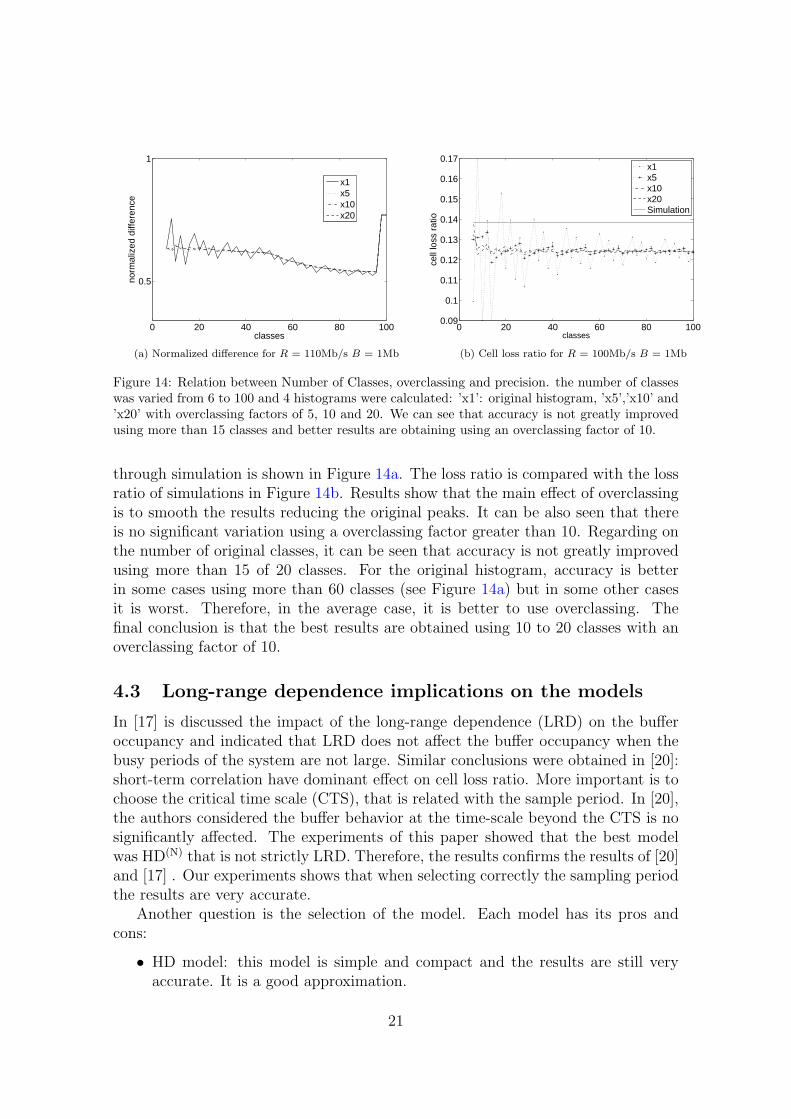
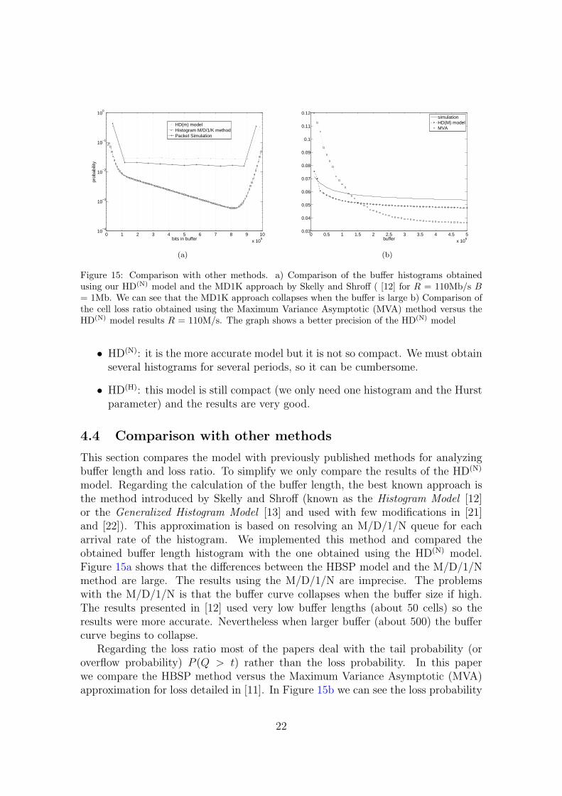
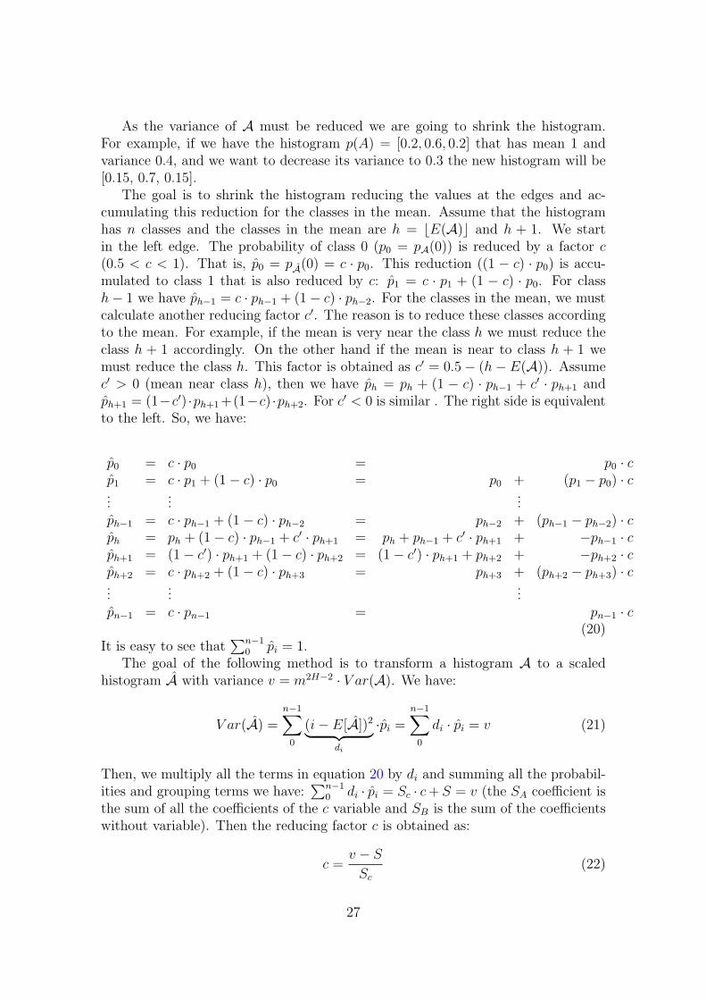
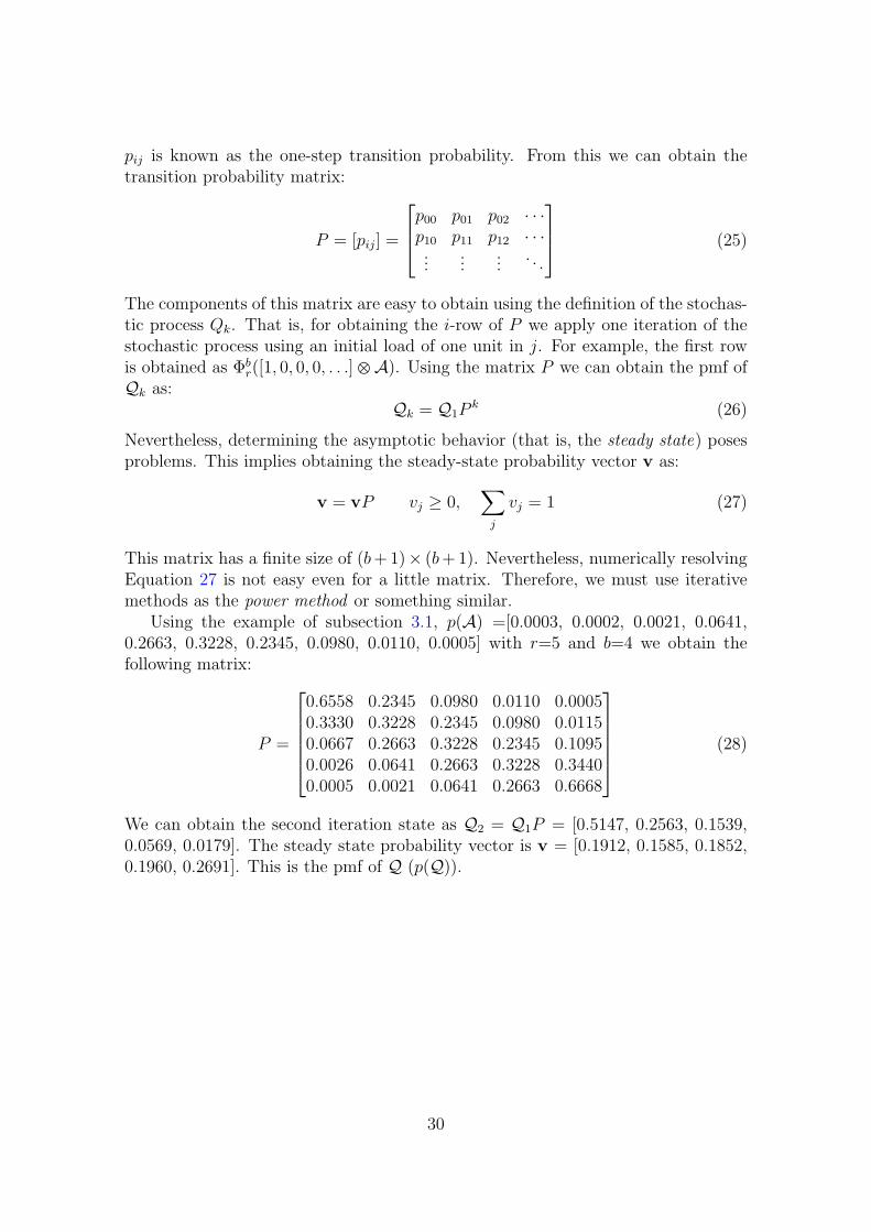