network neighborhood analysis for detecting …
TRANSCRIPT

NETWORK NEIGHBORHOOD ANALYSIS FOR DETECTING ANOMALIESIN TIME SERIES OF GRAPHS
by
Suchismita GoswamiA Dissertation
Submitted to theGraduate Faculty
ofGeorge Mason UniversityIn Partial fulfillment of
The Requirements for the Degreeof
Doctor of PhilosophyComputational Science and Informatics
Committee:
Dr. Igor Griva, Committee Chair
Dr. Edward Wegman, Committee Co-Chair
Dr. Jeff Solka, Committee Member
Dr. Dhafer Marzougui, Committee Member
Dr. Jason Kinser, Acting DepartmentChairperson
Dr. Donna Fox, Associate Dean,Office of Student Affairs & Special Programs,College of Science
Dr. Peggy Agouris, Dean, College of Science
Date: Spring Semester 2019George Mason UniversityFairfax, VA

Network Neighborhood Analysis For Detecting Anomalies in Time Series of Graphs
A dissertation submitted in partial fulfillment of the requirements for the degree ofDoctor of Philosophy at George Mason University
By
Suchismita GoswamiMaster of Science
George Mason University, 2013Master of Science
State University of New York, Stony Brook, 2001
Chair: Dr. Igor Griva, ProfessorDepartment of Computational and Data Sciences
Spring Semester 2019George Mason University
Fairfax, VA

Copyright c© 2019 by Suchismita GoswamiAll Rights Reserved
ii

Dedication
I dedicate this dissertation to my parents, Professor Rabindranath Ganguli and BasantiGanguli.
iii

Acknowledgments
I would not have done this research work without the great teachers in my undergraduateand graduate courses. In particular, I would like to thank Dr. Stephen Finch at SUNY,Stony Brook, Dr. Clifton D. Sutton at GMU, Dr. Bijoy Biswas and Dr. Probodh Bhowmicat Krishnath College, Berhampore, India, who made this possible.
I would like to thank my dissertation director and adviser Dr. Edward J. Wegman forhis support and guidance, and for making this work possible. I also thank him for sug-gesting this work and providing me with the data. I am also thankful to him for providingme the opportunity to present this work at the Symposium on Data Science and Statistics(SDSS) in May 2018 in Reston, VA, and at the International Conference on Computational
Social Science (IC2S2-2018), Kellogg School of Management at North Western University,Chicago. In addition, I thank my committee members, Dr. Igor Griva, Dr. Jeff Solka andDr. Dhafer Marzougui, for their encouragements and suggestions.
I would like to thank Dr. Edward Wegman for offering Measure theory and LinearSpace, Data Mining, and Text Mining, Dr. Clifton Sutton for Applied Statistics, and Sta-tistical Inference, Dr. James Gentle for Time Series Analysis, and Dr. Yunpeng Zhao forNetwork Modeling. Those courses helped me enormously in carrying out this research work.
I would like to thank my mother, Basanti Ganguli and my father, Professor RabindranathGanguli, who is my friend, philosopher and guide, for encouraging me to pursue a PhD. Myfather taught me how to be mindful, which helped me enormously to carry out my PhDstudies. I remember that he used to recite a Sloka written in Sanskrit, ...’Gururevo ParamBrahma, Tasmai Shree Gurave Nama’, which can be approximately translated as Gurus orTeachers are the supreme beings or enlightened persons, and I bow down or salute thoseGurus.
I would like to thank my friends and classmates at GMU, at SUNY at Stony Brook, andat Krishnath College, Berhampore, India for their encouragements. In addition, I wouldlike to thank my sisters, Mithu and Mita, for their support at various stages of my academicpursuits. Lastly, I would like to give a big THANK to Ramasis for giving me the supportand the encouragement, for telling me every morning to stay focused and positive, andalways being there during my PhD studies. I couldn’t have come this far without you.
iv

Table of Contents
Page
List of Tables . . . . . . . . . . . . . . . . . . . . . . . . . . . . . . . . . . . . . . . . viii
List of Figures . . . . . . . . . . . . . . . . . . . . . . . . . . . . . . . . . . . . . . . . x
Abstract . . . . . . . . . . . . . . . . . . . . . . . . . . . . . . . . . . . . . . . . . . . xv
1 Introduction . . . . . . . . . . . . . . . . . . . . . . . . . . . . . . . . . . . . . . 1
1.1 Prior Work on Network Data Using Scan Statistics . . . . . . . . . . . . . . 3
1.2 Present Research . . . . . . . . . . . . . . . . . . . . . . . . . . . . . . . . . 6
1.3 Distribution of Scan Statistic . . . . . . . . . . . . . . . . . . . . . . . . . . 9
1.3.1 Exact Distribution . . . . . . . . . . . . . . . . . . . . . . . . . . . . 9
1.3.2 Order Statistics and Extreme Value Theory . . . . . . . . . . . . . . 11
1.4 The Critical Region . . . . . . . . . . . . . . . . . . . . . . . . . . . . . . . 13
1.5 Time Series . . . . . . . . . . . . . . . . . . . . . . . . . . . . . . . . . . . . 14
1.6 Graph Features: Degree, Betweenness and Density . . . . . . . . . . . . . . 18
1.7 Different Surveillance Methods . . . . . . . . . . . . . . . . . . . . . . . . . 19
1.8 Chapter Summary and Layouts . . . . . . . . . . . . . . . . . . . . . . . . . 20
2 Neighborhood Analysis using Scan Statistics . . . . . . . . . . . . . . . . . . . . 22
2.1 Introduction . . . . . . . . . . . . . . . . . . . . . . . . . . . . . . . . . . . . 22
2.2 Detection of Change Point in Time Series of Raw E-Mail Count . . . . . . . 24
2.3 Discrete Scan Statistics Using Poisson Process . . . . . . . . . . . . . . . . 26
2.4 Detection of Cluster of Communications Using Two-Step Scan Process . . . 29
2.4.1 Removal of Trend and Seasonal Effects . . . . . . . . . . . . . . . . . 29
2.4.2 Step-I of Two-Step Scan Process: Estimation of LLR using Poisson
Model . . . . . . . . . . . . . . . . . . . . . . . . . . . . . . . . . . . 33
2.5 Step-II of Two-Step Scan Process: Network Neighborhood Analysis . . . . . 36
2.5.1 Data Processing . . . . . . . . . . . . . . . . . . . . . . . . . . . . . 36
2.5.2 Formation of Ego Subnetworks Around Most Likely Cluster . . . . . 39
2.5.3 Estimation of LLR Using Binomial Model . . . . . . . . . . . . . . . 42
2.5.4 Maximum Likelihood Estimation Using Non-Parametric Model . . . 45
2.6 Monte Carlo Simulation . . . . . . . . . . . . . . . . . . . . . . . . . . . . . 48
2.6.1 Evaluation of Performance of Scan Statistic Model . . . . . . . . . . 50
v

2.7 Chapter Summary . . . . . . . . . . . . . . . . . . . . . . . . . . . . . . . . 52
3 Anomaly Detection Using Univariate and Multivariate Time Series Models . . . 54
3.1 Introduction . . . . . . . . . . . . . . . . . . . . . . . . . . . . . . . . . . . . 54
3.2 Univariate Time Series from e-mail Networks . . . . . . . . . . . . . . . . . 55
3.2.1 Graph Distance Metrics . . . . . . . . . . . . . . . . . . . . . . . . . 55
3.2.2 Graph Edit Distance to Time Series . . . . . . . . . . . . . . . . . . 55
3.2.3 AR model . . . . . . . . . . . . . . . . . . . . . . . . . . . . . . . . . 56
3.2.4 MA model . . . . . . . . . . . . . . . . . . . . . . . . . . . . . . . . . 58
3.2.5 ARMA model . . . . . . . . . . . . . . . . . . . . . . . . . . . . . . . 59
3.3 Estimation of Parameters . . . . . . . . . . . . . . . . . . . . . . . . . . . . 59
3.3.1 Maximum Likelihood for ARMA(p,q) Process . . . . . . . . . . . . . 59
3.3.2 Yule-Walker Estimation for an AR(p) Process . . . . . . . . . . . . . 61
3.3.3 Estimation Method for MA(1) Process . . . . . . . . . . . . . . . . 63
3.4 Excessive Activities and Residuals . . . . . . . . . . . . . . . . . . . . . . . 65
3.5 Graph Edit Distance to Multiple Time Series . . . . . . . . . . . . . . . . . 67
3.6 Variable Selection of the VAR model . . . . . . . . . . . . . . . . . . . . . . 70
3.7 Vector Autoregressive Model . . . . . . . . . . . . . . . . . . . . . . . . . . 72
3.7.1 Bivariate VAR(1) Model . . . . . . . . . . . . . . . . . . . . . . . . . 78
3.8 The Stationarity of Time Series . . . . . . . . . . . . . . . . . . . . . . . . . 79
3.8.1 Stationarity Condition . . . . . . . . . . . . . . . . . . . . . . . . . . 79
3.8.2 Stationarity Condition: ADF Tests . . . . . . . . . . . . . . . . . . . 80
3.8.3 Estimation of Parameters: Multivariate . . . . . . . . . . . . . . . . 83
3.8.4 Information Criteria for Order Selection of VAR Model . . . . . . . 87
3.9 Excessive Activities Using Residual Analysis of VAR(1) Model . . . . . . . 89
3.10 Detecting Chatter . . . . . . . . . . . . . . . . . . . . . . . . . . . . . . . . 92
3.11 Chapter Summary . . . . . . . . . . . . . . . . . . . . . . . . . . . . . . . . 96
4 Pattern Retrieval and Anomaly Detection from E-Mail Content . . . . . . . . . . 98
4.1 Introduction . . . . . . . . . . . . . . . . . . . . . . . . . . . . . . . . . . . . 98
4.2 Content Analysis and Anomaly . . . . . . . . . . . . . . . . . . . . . . . . . 99
4.3 Documents Preprocessing . . . . . . . . . . . . . . . . . . . . . . . . . . . . 100
4.4 The Term Document Matrix . . . . . . . . . . . . . . . . . . . . . . . . . . . 101
4.5 Document Similarity . . . . . . . . . . . . . . . . . . . . . . . . . . . . . . . 102
4.5.1 Multidimensional Scaling (MDS) . . . . . . . . . . . . . . . . . . . . 103
4.5.2 Singular Value Decomposition (SVD) . . . . . . . . . . . . . . . . . 105
4.6 Latent Dirichtlet Allocation Method (LDA) . . . . . . . . . . . . . . . . . . 106
vi

4.6.1 Parameters estimation: Gibbs sampling . . . . . . . . . . . . . . . . 107
4.7 Evolution of Topics Across Time Using LDA . . . . . . . . . . . . . . . . . 108
4.8 Clustering . . . . . . . . . . . . . . . . . . . . . . . . . . . . . . . . . . . . . 112
4.9 Scan Statistics on Topic Proportions Using Normal Distribution . . . . . . 117
4.10 Time Series Models on Topic 1: Compositional ARIMA (C-ARIMA) Model 121
4.11 Identifying Vertices with Excessive Messages using a Combination of 1-Nearest
Neighbor (1NN) and K-Means . . . . . . . . . . . . . . . . . . . . . . . . . . 124
4.12 Chapter Summary . . . . . . . . . . . . . . . . . . . . . . . . . . . . . . . . 126
5 Conclusions . . . . . . . . . . . . . . . . . . . . . . . . . . . . . . . . . . . . . . . 134
5.1 Summary of Contributions . . . . . . . . . . . . . . . . . . . . . . . . . . . . 134
5.2 Future Work . . . . . . . . . . . . . . . . . . . . . . . . . . . . . . . . . . . 138
6 Appendix A . . . . . . . . . . . . . . . . . . . . . . . . . . . . . . . . . . . . . . 140
7 Appendix B . . . . . . . . . . . . . . . . . . . . . . . . . . . . . . . . . . . . . . . 147
Bibliography . . . . . . . . . . . . . . . . . . . . . . . . . . . . . . . . . . . . . . . . . 151
vii

List of Tables
Table Page
2.1 Kolmogorov Smirnov Test Statistics for different bandwidth parameters, Ob-
served values and critical values. . . . . . . . . . . . . . . . . . . . . . . . . 27
2.2 Temporal clusters of email count showing the estimated maximum loglikeli-
hood ratio (LLR), standard Monte critical values (SMCV), Gumbel critical
values (GCV) and significance level (SL) obtained using SaTSscan software. 35
2.3 The maximum log likelihood ratio at week 20 and week 21 respectively with
Gumbel critical values (GCV), standard Monte critical values (SMCV), and
significance level (SL) for k = 1.5, 2.0 and > 2.0 using the Binomial model. 44
2.4 Empirical sizes (in percentage) for the LLR in testing for a cluster of events
for scan statistic model. . . . . . . . . . . . . . . . . . . . . . . . . . . . . . 52
2.5 The simulated critical values for the LLR for n = 1000. . . . . . . . . . . . 53
3.1 The order of a graph G, the order of graph H, the size of graph G, size of a
graph H, and the graph edit distance between two graphs, G and H. . . . . 57
3.2 Tests for unit roots showing that the time series is stationary. . . . . . . . . 58
3.3 The estimated parameters and AIC of ARMA models. . . . . . . . . . . . . 64
3.4 Roots of the characteristic polynomial for k = 1, 1.5 and 2. . . . . . . . . . . 80
3.5 Critical values for the ADF tests for the GED series of ID = 1, 5, 7, 10 and
20 for k = 1, 1.5 and 2. . . . . . . . . . . . . . . . . . . . . . . . . . . . . . 84
3.6 Information Criteria for the VAR(p) model selection for k = 2. . . . . . . . 89
3.7 Excessive activity for k = 1, 1.5 and 2. . . . . . . . . . . . . . . . . . . . . 93
3.8 Multivariate Portmanteau statistics of GED for k = 2. . . . . . . . . . . . . 97
4.1 A partial document term matrix for e-mail content from June 2003 to June
2004 around the primary cluster obtained from scan statistics showing the
frequency of words in documents. . . . . . . . . . . . . . . . . . . . . . . . . 103
4.2 The partial document-topic matrix. . . . . . . . . . . . . . . . . . . . . . . . 113
4.3 The partial T 52×19 matrix of e-mail content. . . . . . . . . . . . . . . . . . 113
4.4 The partial S19×19 matrix of e-mail content. . . . . . . . . . . . . . . . . . 114
viii

4.5 The partial (D19×19)T matrix of e-mail content. . . . . . . . . . . . . . . . 115
4.6 Three major topics with top six terms obtained using the LDA from e-mail
content around the most likely cluster. . . . . . . . . . . . . . . . . . . . . . 116
4.7 Topic probabilities by document obtained using the LDA method. . . . . . 129
4.8 Topic probabilities by document: Continued. . . . . . . . . . . . . . . . . . 130
4.9 Unit root tests on the transformed maximum topic proportion. . . . . . . . 131
4.10 Temporal clusters of the topic proportion showing the estimated log likeli-
hood ratio (LLR), standard Monte critical values (SMCV) and significance
level (SL) obtained using SaTSscan software. . . . . . . . . . . . . . . . . . 131
4.11 Unit root tests for logit (p). . . . . . . . . . . . . . . . . . . . . . . . . . . . 131
4.12 Unit root tests for the first difference logit (p) series. . . . . . . . . . . . . . 132
4.13 ARIMA(0,1,1), ARIMA(1,1,0) and ARIMA(1,1,1) model results fitted to the
logit of topic 1 proportion series. . . . . . . . . . . . . . . . . . . . . . . . . 132
4.14 Proportion of massages obtained from the combination of K-means and near-
est neighbor. . . . . . . . . . . . . . . . . . . . . . . . . . . . . . . . . . . . 133
ix

List of Figures
Figure Page
2.1 (a) Monthly number of e-mails received for the period 1996-2009. (b,c) Sam-
ple ACF and PACF of the monthly number of e-mails, respectively, showing
that the time series is not stationary. . . . . . . . . . . . . . . . . . . . . . . 28
2.2 Scatter plot matrix showing the correlation of e-mail count with its own
lagged values. . . . . . . . . . . . . . . . . . . . . . . . . . . . . . . . . . . . 30
2.3 The time plot of the natural logarithm showing the change in mean. . . . . 31
2.4 (a) Kernel smoothing of the raw e-mail count data showing an upward trend.
(b) Plot showing the seasonal variations of the raw e-mail count data. . . . 32
2.5 (a) Time plot of email count after removing the trend and seasonal variation
by seasonal differencing. Note the change in the mean is removed. (b) The
sample ACF (top right) and PACF (lower right)of seasonally adjusted and
trend removed email count series. . . . . . . . . . . . . . . . . . . . . . . . . 34
2.6 The primary and secondary clusters, obtained using SatScan software, are
shown by rectangular boxes in the count series (upper panel). The LLR esti-
mated as a function of variable and overlapping bin w, showing the primary
and secondary clusters at the same time period (lower panel). . . . . . . . . 36
2.7 The weekly subnetworks obtained from e-mails for the period September
2003-October 2003. . . . . . . . . . . . . . . . . . . . . . . . . . . . . . . . . 38
2.8 Weekly neighborhood ego subnetworks with maximum betweenness for k =
1.5 for the 32 week period in 2003 around the primary cluster obtained using
Poisson model. . . . . . . . . . . . . . . . . . . . . . . . . . . . . . . . . . . 39
2.9 Weekly maximum betweenness series for k = 1 (top), 1.5 (upper middle), 2
(lower middle) and > 2 (lower). . . . . . . . . . . . . . . . . . . . . . . . . . 40
2.10 The sample ACF of the weekly maximum betweenness series for k = 1 (top),
1.5 (upper middle), 2 (lower middle) and ¿2 (lower). . . . . . . . . . . . . . 41
x

2.11 The estimated LLR as a function of variable and overlapping w for k =
1.5(top panel), 2(middle panel), > 2 (lower panel) for the 32 week period in
2003 around the primary cluster. . . . . . . . . . . . . . . . . . . . . . . . . 44
2.12 The anomalous ego sub network with ID = 15 (upper panel) detected at week
t = 20 in 2003 for k = 1.5 (top left), k = 2(middle) and k = > 2 (top right).
The vertex has maximum absolute betweenness score. Neighborhood ego sub
networks with the second maximum absolute betweenness score (lower panel)
for ID = 5. . . . . . . . . . . . . . . . . . . . . . . . . . . . . . . . . . . . . 45
2.13 Circular plot showing ID = 15 associated with the maximum betweenness in
the middle. . . . . . . . . . . . . . . . . . . . . . . . . . . . . . . . . . . . . 46
2.14 (a) The estimated pmf of the maximum betweenness as a function of ordered
observations. (b) The estimated density with mode placed at the smallest
order statistic. (c) The estimated density with mode placed at the largest
order statistic. . . . . . . . . . . . . . . . . . . . . . . . . . . . . . . . . . . 47
2.15 The Log likelihood estimate using a non-parametric method as a function of
mode. . . . . . . . . . . . . . . . . . . . . . . . . . . . . . . . . . . . . . . . 48
2.16 The estimated power for the Log likelihood ratio as a function of λ. . . . . 51
3.1 Weekly subnetworks at different time points. The GED was estimated from
adjacent periods to compare subgraphs sequentially. . . . . . . . . . . . . . 56
3.2 (a)Time Plots of observed and fitted GED series using ARMA Model for the
52 week period June 2003 - June 2004. (b) The sample ACF (top panel) and
the sample PACF (lower panel) of weekly GED series for the 52 week period
June 2003 - June 2004, respectively. . . . . . . . . . . . . . . . . . . . . . . 57
3.3 The standardized residual series (upper panel) for the MA(1)fit to the GED
series and the ACF of standardized residuals for the MA(1) fit to the GED se-
ries (middle panel), and p-values for the Ljung-Box-Pierce Q-statistic (lower
panel for the MA(1) fit to the GED series). . . . . . . . . . . . . . . . . . . 64
3.4 The histogram of the residuals (upper panel) and the Normal Q-Q plot of
the residuals of the MA(1) fit to the GED series (lower panel), showing the
residuals are close to normality except for an extreme value in the right tail. 66
3.5 The neighborhood ego networks for k = 1 for ID = 5 for the 52 week period,
June 2003 - June 2004. . . . . . . . . . . . . . . . . . . . . . . . . . . . . . . 67
xi

3.6 The neighborhood ego networks for k = 1.5 for ID = 5 for the 52 week period,
June 2003 - June 2004 around the primary cluster estimated from monthly
temporal scan statistic model. . . . . . . . . . . . . . . . . . . . . . . . . . . 68
3.7 (a) Weekly GED series estimated from adjacent periods to compare sub-
graphs sequentially with missing values for ID = 1. Weekly GED series for
ID = 1 (lower panel) after the imputation of missing values with mean. (b)
The time plots of GED with different imputation methods for ID = 1. . . . 69
3.8 (a) A five-dimensional GED series for IDs = 1, 5, 7, 10 and 20 for k = 1.0.
Note the spike at week = 20 for ID = 5. (b) The univariate GED series
plotted separately for these IDs. . . . . . . . . . . . . . . . . . . . . . . . . 70
3.9 (a) A five-dimensional GED series for IDs = 1, 5, 7, 10 and 20 for k = 1.5.
Note the spike at week = 20 for IDs = 5 and 7. (b) The univariate GED
series plotted separately for these IDs. . . . . . . . . . . . . . . . . . . . . . 71
3.10 (a) A five-dimensional GED series for IDs = 1,5, 7, 10 and 20 for k = 2.0.
Note the spike at week = 20 for IDs = 5 and 7. (b) The univariate GED
series plotted separately for these IDs. . . . . . . . . . . . . . . . . . . . . . 72
3.11 (a,b,c) Correlation bar plots of the GED for ID = 1, 5, 7, 10 and 20 with
k = 1, 1.5 and 2, respectively. . . . . . . . . . . . . . . . . . . . . . . . . . . 73
3.12 A scatterplot matrix of five-dimensional GED data illustrating correlations
for k = 2. . . . . . . . . . . . . . . . . . . . . . . . . . . . . . . . . . . . . . 74
3.13 (a,b,c) Parallel coordinate plot of five-dimensional GED data showing corre-
lations for k = 1, k = 1.5, and k = 2 respectively. . . . . . . . . . . . . . . 75
3.14 (a) Weekly GED series for IDs = 1,5, 7, 10 and 20 for k = 1.0 with kernel
smoothing, showing no trend in the kernel fit to the series. . . . . . . . . . . 76
3.15 (a) Weekly GED series for IDs = 1, 5, 7, 10 and 20 for k = 2.0 with kernel
smoothing, showing no trend in the kernel fit to the series. . . . . . . . . . . 77
3.16 The ACF and PACF plots of the weekly GED series for IDs = 1,5, 7, 10 and
20 for k = 1.0, showing the series is stationary. . . . . . . . . . . . . . . . . 82
3.17 The ACF and PACF plots of the weekly GED series for IDs = 1, 5, 7, 10
and 20 for k = 2.0, showing the series is stationary. . . . . . . . . . . . . . . 83
3.18 (a,b) The information criteria for the VAR models fitted to 5-dimensional
series showing that the AIC, BIC and HQ are minimized when the order is
1 for k = 1 and 2, respectively. . . . . . . . . . . . . . . . . . . . . . . . . . 86
xii

3.19 (a) Time plots of observed and fitted GED series (upper panel) and residual
series (middle panel) of the VAR(1) model fit to the 5-dimensional GED
series of ID = 1, 5, 7, 10 and 20 for k = 1.0. The ACF and PACF of the
residuals are shown in the lower panel. . . . . . . . . . . . . . . . . . . . . . 91
3.20 (a) Plots showing the fit (upper panel) and residual (middle panel) for the
VAR(1) fit to the 5-dimensional GED series of ID = 1, 5, 7, 10 and 20 for
k = 2.0. The ACF and PACF of the residuals are shown in the lower panel. 92
3.21 (a) The residual cross-correlation matrices for the VAR(1) model fit to the
5-dimensional GED series of ID = 1, 5, 7, 10 and 20 for k = 2.0. . . . . . . 93
3.22 (a,b) The p-values of the multivariate Ljung-Box statistics (Qk(m)) applied
to the residuals of the VAR(1) model fit to the 5-dimensional GED series of
ID = 1, 5, 7, 10 and 20 for k = 1 and 2, respectively. . . . . . . . . . . . . . 94
3.23 Time plots of the residuals for the VAR(1) model fit to the 5-dimensional
GED series of ID = 1, 5, 7, 10 and 20 for k = 2.0. The chatter is detected at
week = 20. The dotted red line corresponds to the residual exceeding 2.5σ
standard deviations above the mean. . . . . . . . . . . . . . . . . . . . . . 95
4.1 Histogram showing frequency of words after denoising and stemming. . . . 102
4.2 Model selection using the log likelihood for the number of topics showing
that it does not converge to a global maximum with the increase of number
of topics. . . . . . . . . . . . . . . . . . . . . . . . . . . . . . . . . . . . . . 109
4.3 Model selection using the information criteria for the number of topics. . . . 110
4.4 (a,b) Multidimensional scaling for the original 52 X 10315 DTM, showing 3
major dimensions. The largest dimension is 19. . . . . . . . . . . . . . . . 111
4.5 (a,b) Singular value decomposition for the original 52 x 10315 DTM, showing
3 dimensions. . . . . . . . . . . . . . . . . . . . . . . . . . . . . . . . . . . . 112
4.6 (a) Topic proportion of all three topics for the 52 week period around the
primary cluster using scan statistic model. (b) Topic proportion plotted
separately with time. . . . . . . . . . . . . . . . . . . . . . . . . . . . . . . . 114
4.7 Hierarchical agglomerative clustering on the document term matrix, showing
the dendrogram with three major clusters using the single link method. . . 116
4.8 K-means clustering showing three clusters. . . . . . . . . . . . . . . . . . . . 117
xiii

4.9 (a) The maximum proportion of topics for the 52 week period around the
primary cluster using scan statistic model . (b) The logistic transformed
maximum proportion of topics for the 52 week period around the primary
cluster using scan statistic model. . . . . . . . . . . . . . . . . . . . . . . . . 121
4.10 A normal Q-Q plot of the logistic transformed maximum proportion of topics
showing that the distribution is approximately normal. . . . . . . . . . . . . 122
4.11 Sample ACF and PACF of the logistic transformed maximum proportion of
topics series showing that the time series is stationary. . . . . . . . . . . . . 123
4.12 The observed and fitted logistic transformed proportion of topic 1 series for
the ARIMA(0,1,1) fit to the logistic transformed proportion of topic 1 series. 124
4.13 Time Plots of the standardized residuals, the ACF of standardized residual
and the Q-statistic for the ARIMA(0,1,1) fit to the transformed topic 1. . . 125
4.14 Histogram of the residuals (top), and a normal Q-Q plot of the residuals
(bottom) for the ARIMA(0,1,1) fit to the logistic transformed proportion of
topic 1 series. . . . . . . . . . . . . . . . . . . . . . . . . . . . . . . . . . . . 126
4.15 Comparison between time plots of betweenness for k > 2 for different IDs
obtained from metadata, and the maximum topic proportion obtained from
LDA using textual data, showing that the excessive topic activity relating to
the topic 1, which is associated with ID = 5, 7, 18, 20 and 30 at around week
20. . . . . . . . . . . . . . . . . . . . . . . . . . . . . . . . . . . . . . . . . . 127
xiv

Abstract
NETWORK NEIGHBORHOOD ANALYSIS FOR DETECTING ANOMALIES IN TIMESERIES OF GRAPHS
Suchismita Goswami, PhD
George Mason University, 2019
Dissertation Director: Dr. Igor Griva
Around terabytes of unstructured electronic data are generated every day from twitter
networks, scientific collaborations, organizational emails, telephone calls and websites. Ex-
cessive communications in communication networks, particularly in organizational e-mail
networks, continue to be a major problem. In some cases, for example, Enron e-mails,
frequent contact or excessive activities on interconnected networks lead to fraudulent activ-
ities. Analyzing the excessive activity in a social network is thus important to understand
the behavior of individuals in subregions of a network. In a social network, anomalies can
occur as a result of abrupt changes in the interactions among a group of individuals. There-
fore, one needs to develop methodologies to analyze and detect excessive communications
in dynamic social networks. The motivation of this research work is to investigate the ex-
cessive activities and make inferences in dynamic sub networks. In this dissertation work,
I implement new methodologies and techniques to detect excessive communications, topic
activities and the associated influential individuals in the dynamic networks obtained from
organizational emails using scan statistics, multivariate time series models and probabilistic
topic modeling. Three major contributions have been presented here to detect anomalies
of dynamic networks obtained from organizational emails.

At first, I develop a different approach by invoking the log-likelihood ratio as a scan
statistic with overlapping and variable window sizes to rank the clusters, and devise a
two-step scan process to detect the excessive activities in an organizations e-mail network
as a case study. The initial step is to determine the structural stability of the e-mail
count time series and perform differencing and de-seasonalizing operations to make the
time series stationary, and obtain a primary cluster using a Poisson process model. I then
extract neighborhood ego subnetworks around the observed primary cluster to obtain more
refined cluster by invoking the graph invariant betweenness as the locality statistic using the
binomial model. I demonstrate that the two-step scan statistics algorithm is more scalable
in detecting excessive activity in large dynamic social networks.
Secondly, I implement for the first time the multivariate time series models to detect
a group of influential people and their dynamic relationships that are associated with ex-
cessive communications, which cannot be assessed using scan statistics models. For the
multivariate modeling, a vector auto regressive (VAR) model has been employed in time
series of subgraphs in e-mail networks constructed using the graph edit distance, as the
nodes or vertices of the subgraphs are interrelated. Anomalies or excessive communications
are assessed using the residual thresholds greater than three times the standard deviations,
obtained from the fitted time series models.
Finally, I devise a new method of detecting excessive topic activities from the unstruc-
tured text obtained from e-mail contents by combining the probabilistic topic modeling
and scan statistics algorithms. Initially, I investigate the major topics discussed using the
probabilistic modeling, such as latent Dirichlet allocation (LDA) modeling, then employ
scan statistics to assess the excessive topic activities, which has the largest log likelihood
ratio in the neighborhood of primary cluster.
These analyses provide new ways of detecting the excessive communications and topic
flow through the influential vertices in a dynamic network, and can be extended in other
dynamic social networks to critically investigate excessive activities.

Chapter 1: Introduction
Anomalies, which are clusters of events or excessive or unusual activities, are common in
science and technology. Some of the most commonly used methods for anomaly detec-
tion in data mining are density-based techniques such as k-nearest neighbor [KNT00] and
local outlier factor [BKNS00], one class support vector machines [SPST+01], neural net-
works [HHWB00], cluster analysis-based outlier detection [HXD03] and ensemble techniques
[LK05]. All these methods used to detect excessive activity, are mostly descriptive in na-
ture, and not effective in making statistical inferences. In other words, these methods do
not predict if these observed clusters of events are statistically significant or not [Kul79].
A very powerful statistical inference methodology that has been developed to detect the
region of unusual activity in a random process and to infer the statistical significance of
the observed excessive activity is scan statistics [Kul79], which is also termed as moving
window analysis in the engineering literature and has mostly been used in spatial statistics
and image analysis.
Scan statistic is defined as a maximum or minimum of local statistics estimated from
the local region of the data. Let Xt, t ≥ 0 be a Poisson process with rate, λ, where Xt is
the number of points (events) occurring in the interval [0, t). In any subinterval of [0, T)
of length, w, let Yt be the number of points (events) in a window of the interval, [t, t+ w),
such that Yt = Xt+w - Xt. The one-dimensional continuous scan statistic, Sw, is written as
[GB99]:
Sw = max0<t≤T−w
Yt(w). (1.1)
In other words, the scan statistic, Sw, is the largest number of points that are observed in
any subinterval of [0, T) of length w. In this Poisson process, λ is the expected (average)
1

number of events in any unit interval and the number of points (events) in any interval,
[t, t + w), Yt follows a Poisson distribution with mean λw. The probability mass function
for the random variable, Yt, can be written as:
P (Yt(w) = k) =e−λw(λw)k
k!. (1.2)
In one-dimensional setting, it has been used by a number of authors to investigate the un-
usual clusters of events in various fields, for example, in visual perception [Gla79], molecular
biology [KB92], epidemiology [WN87], queueing theory [Gla81], material science [New63],
and telecommunication [Alm83]. Public health officials are often interested in finding expla-
nations of clusters of cancer cases. Kulldorff et al. [Kul79] have assessed the unusually large
number of brain cancer cases using spatial scan statistics. In medical imaging or screening
situation, detection of abnormalities in structural images is very important. In this situ-
ation, a one-dimensional scan statistic model may not be adequate for cluster detection.
It is, therefore, extended to two or three dimensional settings to study the mammography
images. Priebe et al. [POH98] have exploited the stochastic scan partitions in the mam-
mography images by studying the texture of the breast, and evaluated clusters of breast
calcification using spatial scan statistics, and provided an exact sampling distribution of the
spatial scan statistic under the null hypothesis of homogeneity. For the non-homogeneous
mammogram, a p value of 0.034 has been reported by Priebe et al [POH98].
Although considerable work has been done to detect clusters of events or anomaly using
scan statistics in spatial statistics and image analysis, relatively less attention has been given
to detect anomaly in social networks, where lots of interaction take place among individuals
or group of individuals. In addition to sharing knowledge and experience with one another
in social networks, each individual develops a pattern of interactions. Anomaly in social
network occurs when some individuals or group of individuals make sudden changes in their
patterns of interactions. Research on social networks includes both static and dynamic social
relations. Methods and theorems from graph theory and statistics are used intensively in
2

analyzing social networks. Despite the fact that the majority of research focuses greatly on
static networks, they fail to capture information flow in dynamic networks.
Recently, a number of measures and algorithms have been developed for dichotomous
and symmetric relation matrices in the analysis of dynamic networks. As the amount
of unstructured electronic data created by various social networks, for example, twitter
network, research network, a network of scientific collaboration, organizational e-mails and
telephone calls increases enormously to terabyte range day by day, the need for tools and
techniques to analyze such unstructured massive data sets has grown. In some cases, one
needs to analyze the excessive activity in a social network to understand the behavior of the
network. The motivation of this research work is to investigate the excessive activities in
the network data from organizational e-mails by implementing statistical models and data
mining algorithms, particularly scan statistics, time series models and content analysis. The
methodologies developed here can be applied to other dynamic networks to assess excessive
activities in the network.
1.1 Prior Work on Network Data Using Scan Statistics
Priebe et al. [PCMP05] first applied temporal scan statistics to network data to detect
anomaly in time series of graphs, obtained from Enron email data. The full network was
partitioned into disjoint subregions or subnetworks over time, which results in a collection
of graphs or a time series of graphs. The large networks have computational difficulties, and
the visualization and statistical inference are almost impossible to apply to a global network.
An alternating approach to identify interesting features at a specific point of time is to split
the global network as subnetworks or subregions, and consider the network neighborhood
analysis as opposed to global network analysis. The subregions are modeled subsequently
by directed graphs indexed by time, Dt, which are a collection of vertices that are joined
by edges. Graph, Dt, can therefore be expressed as Dt = (V,Et), where each graph has
the same set of vertices, V, and different set of edges, Et. The order of the graph, Dt, is
n = |V | = number of vertices, and size of graph, Dt, is m = |Et| = number of edges. The
3

adjacency matrix of Dt is defined as A = (Aij) such that
Aij =
1, if there is an edge between vertices i and j,
0, otherwise.
From the graph at each time point one can obtain local regions or neighborhoods of vertices.
The kth order neighborhood of a vertex, v, of the network, Dt, is defined as:
Nk[v;Dt] = u ∈ V : dt(u, v) ≤ k; k = 0, 1, 2, .., (1.3)
where dt(u, v) is the geodesic distance, which is in fact the shortest path between u and v
within k. A family of sub graphs induced by neighborhood denoted by Ω(Nk[v;Dt]) with a
set of vertices, Nk[v;Dt], can then be obtained.
To quantify the characteristics of a node in subgraphs, the graph invariant feature, such
as degree, can be used. Priebe et al. [PCMP05] used outdegree as the locality statistics.
The degree of a node in a graph is the number of direct connections incident on it, while in
the directed network, the degree is defined based on both in-degree and out-degree, where
the in-degree is the number of inward edges and the out-degree is the number of outward
edges. Thus, a person having high out-degree will be able to send a lot of information to
other actors in the network. Priebe et al. [PCMP05] defined the locality statistic,Ψk,t(v),
the standardized locality statistic,Ψk,t(v), and the scan statistics, Mk,t, as:
Ψk,t(v) = |E(Ω(Nk[v,Dt]))|; k = 0, 1, 2...; (1.4)
Ψk,t(v) =Ψk,t(v)− µk,t,w(v)
max(1, σk,t,w(v)), (1.5)
Mk,t = maxv∈V
Ψk,t(v); k = 0, 1, 2, ..., (1.6)
4

µk,t,w(v) =1
w
t−1∑j=t−w
Ψk,j(v), (1.7)
σ2k,t,w(v) =
1
w − 1
t−1∑j=t−w
(Ψk,j(v)− µk,t,w(v))2 , (1.8)
where µk,t,w(v) and σ2k,t,w(v) are the mean and the variance, respectively, of the local statistic
in the window w. The standardized scan statistic at the time t is written as:
Mk,t = maxv∈V
Ψk,t(v); k = 0, 1, 2, ... (1.9)
The standardized scan statistic, Mk,t, was further normalized to temporally normalized scan
statistic, Sk,t, which is defined as:
Sk,t =(Mk,t − µk,t,l)max(1, σk,t,l)
, (1.10)
where µk,t,l and σk,t,l are the estimated mean and standard deviation, respectively, of Mk,t
corresponding to the lag or time step l. The Mk,t have been estimated for k = 0, 1, 2 and
t = 1, 2, ..., 189 for the Enron data. For k = 2, t = 132 and l = 20, the Mk,t is greater than
5 times standard deviations above its mean, indicating a clear anomaly. The corresponding
temporally-normalized scan statistic, S(2,132), is 7.3. Assuming normality, the observed p-
value is < 10−10. They also used the extreme value theory, Gumbel model, to estimate the
exceedance probability (p-value), which turned out to be < 10−10. Therefore, they could
infer using scan statistics that there exist anomalies in the Enron network data.
However, to implement scan statistic, a vertex-dependent local stationarity assumption
was required. The previous model is an oversimplified statistical inference model, and
a short-time near stationary (lag = 20 weeks) for null model was assumed. They did
not consider detrending and seasonal adjustment methods on the univariate time series to
5

make the time series stationary. If xt is a stationary time series, then the distribution of
(xt, ..., xt+s) does not depend on t for all s. As the data are often non-stationary/non-
random, they can give rise to trends and non-constant variance over time. It is also very
common for dynamic email data to have seasonal effect, which can mask the non-seasonal
characteristics of the data. In order to better reveal the features of the data that are of
interest, removing trends, non-constant variance, and seasonal effects from time series data
are necessary.
To obtain temporal scan statistic, Sk,t, Priebe et al. [PCMP05] normalized the locality
statistic, Ψk,t(v), twice and obtained the p-value, assuming normality of the scan statistic.
In this model, it was assumed that the subgraphs are disjoint. However, the anomaly may
split among multiple windows, and the set of subgraphs may not be disjoint, suggesting
that the temporally-normalized scan statistic, Sk,t, is not independent.
They used the outdegree as a locality statistic. The degree, however, is not an effective
structural location of a node in a network. The degree of a node in a graph is the number
of direct connections that a node has with other nodes. If a node has high degree, the
individual will be simply a connector or a hub and will not play a vital role in the social
network. As a result, this metric is not very effective in detecting anomaly in a social
network. On the other hand, the betweenness of a node in global network measures its
influential position (broker, leader or bridge) in the network [PS00]. Thus, the betweenness
centrality applied to neighborhood network can be very useful in identifying locally impor-
tant individuals. Another measure for locality statistics is density applied to neighborhood
network, which reveals how tightly-coupled the neighborhood is [PS00]. This will also be
effective in detecting anomaly of a network.
1.2 Present Research
The objective of this research is to develop a fundamental understanding of methodologies
to discover network patterns, to detect anomalies of dynamic networks obtained from an
6

organizational email, and to make statistical inferences by implementing statistical models
and data mining algorithms. The current research employs temporal scan statistics to detect
clusters, where the maximum log likelihood ratio is the test statistic [Kul79], and use the
betweenness as the locality statistic. Here the betweenness follows a binomial distribution
as it is related to the ratio of number of geodesic paths to the total number of geodesic
paths. In addition, this research develops a purely temporal scan statistics for email count
data based on the Poisson model.
The alternative approaches, such as the autoregressive moving average (ARMA) process
and the vector autoregressive (VAR) process to detect clusters in a point process are imple-
mented for the univariate time series of neighborhood ego subgraphs and the multiple time
series of neighborhood ego subgraphs, respectively. In addition, this research employs the
latent Dirichtlet allocation modeling on the e-mail content to model the topics associated
with the dynamic textual data, and to study any significant topic change associated with
the time series of the maximum topic proportion using scan statistics.
One of the scientific challenges of this research includes understanding the distribution
of the organizational email subnetworks. As in one dimension, the exact distribution of
the scan statistic under the null hypothesis is only available for special cases [PGKS05],
this research employs other methodologies, such as Monte Carlo (MC) simulations and the
extreme value theory to estimate p-values. Once the sampling distribution of scan statistic
is determined, the inference on anomaly can be performed. There are three equivalent ways
of performing a hypothesis test, such as the p-value approach, the classical approach, and
the confidence interval approach. The extreme value theory is a statistical model that is
used to model the extreme data in a given period of time, and is based on the location-
scale family. Gumbel distribution is the most well-known distribution that belongs to this
family, and has been widely used in engineering. The present work also applies the Gumbel
distribution to approximate the p-value.
Another challenge is the choice of local statistic as it provides important structural
location of a node and its neighborhood. I have proposed local graph invariant, such as the
7

betweenness, as a measure to identify local structure in social networks. For building the
univariate time series of graphs, the challenges are to compute the graph distance metrics,
which are computationally intensive, and to fit time series model to assess anomalies based
on residuals.
Technical tasks to meet objectives and scientific challenges of the research are:
1. Scan Statistics: The temporal scan statistics models on email count and network data
over a time interval from an organizational email are developed using the maximum
log-likelihood ratio as the scan statistic. After applying detrending, variance stabi-
lization, and seasonal adjustment to the time series of email count, anomalies have
been assessed. A local statistic for subnetworks, such as betweenness is used. The
extreme value theory and the Monte Carlo simulation methods are employed to make
inferences, as the sampling distribution of the scan statistics is not known for most of
the cases. Also, the Monto Carlo simulations for testing one-change point in mean in
time series of count data is conducted.
2. Time Series: A univariate time series has been developed using the graph edit distance
(GED) between subgraphs. An ARMA model is fitted to the time series, and the
anomalies have been assessed using a residual threshold obtained from the ARMA
model fitted to the GED series. In addition, a VAR model for multivariate time series
of neighborhood ego subnetworks for each vertex using the GED has been developed
to identify anomalies and detect chatter.
3. Content analysis: A vector space model is implemented to construct the term doc-
ument matrix (TDM) obtained from the corpus extracted from unstructured email
content at every week. The probabilistic model, latent Dirichlet allocation (LDA)
process is then applied to the document term matrix (DTM) in order to estimate the
topic proportions to build a univariate time series. Subsequently, anomalies are as-
sessed using scan statistic model and residual analysis of the fitted time series model.
In addition, the multidimensional scaling (MDS) or the singular value decomposition
8

(SVD) is conducted to reduce dimensionality to compare the optimal number of top-
ics obtained from the LDA. The K-means clustering is used to the reduced dimension
obtained from the MDS for the corpus of every vertex at each week to cluster the doc-
uments. Further, the k-nearest neighbor method is implemented to classify messages
at time, t, for pattern retrieval and to identify chatter.
The remainder of this chapter provides an overview on the distribution of the scan
statistics. A brief discussion on the critical region, time series methods, graph properties
are also presented. Finally, an overview of the prospective surveillance methods on the
social network data is presented.
1.3 Distribution of Scan Statistic
1.3.1 Exact Distribution
In one dimension, the exact distribution of the scan statistic is only available for special
cases. Naus [Nau65] has first presented the distribution of the maximum cluster of points
on a line. Here N ordered points, x1 ≤ x2 ≤ . . . ≤ xN , with respect to size are considered
and independently drawn from the uniform distribution on (0, 1). The P (k|N ;w) is the
probability that the largest number of points (events) within a sub interval of (0, 1) of length
w ≥ k. Let Sw be the largest number of points within a sun-interval of [0,1) of length w.
The right tail probability of the scan statistic, Sw, and the P (k|N ;w) are expressed as:
pvalue = P (Sw ≥ k|H0) = P (k|N ;w). (1.11)
Naus [Nau65] has derived the formulas of P (k|N ;w) as:
P (k|N ;w) =
C(k|N ;w)−R(k|N ;w), for w ≥ 1
2 , k >(N+1)
2 ,
C(k|N ;w), for w ≤ 12 , k >
N2 .
9

Here C(k|N ;w) is the sum of cumulative binomial probabilities and defined as:
C(k|N ;w) = (N − k + 1)[Gb(k − 1|N ;w) +Gb(k + 1|N ;w)]− 2(N − k)Gb(k|N ;w), (1.12)
and Gb is the cumulative binomial probability such that:
Gb(k|N ;w) =
N∑i=k
b(i|N ;w), (1.13)
b(k|N ;w) =
(N
k
)wk(1− w)N−k. (1.14)
R(k|N ;w) is the sum of the product of binomials and cumulative binomial probabilities
defined as:
R(k|N ;w) =
N∑i=k
b(y|N ;w)F (N − k|y; v/w) +H(k|N ;w)b(k|N ;w), (1.15)
where
Fb(k|N ;w) =k∑i=0
b(i|N ;w), (1.16)
H(k|N ;w) =nv
wFb(N − k|k − 1; v/w)− (N − k + 1)Fb(N − k + 1|k; v/w), (1.17)
and v = 1 − w. The exact distribution of Sw has been formulated by Wallenstein and
Naus [WN74] and Huntington and Naus [HN75]. Naus [Nau82] has given the following
approximation for a Poisson process with mean rate λ per unit time over the interval [0,T).
For µ = λw and L = Tw :
pvalue = PH0(Sw ≥ k|µ,L) ≈ 1−Q2
(Q3
Q2
)L−2
. (1.18)
10

Q2 and Q3 are defined as:
Q2 = (F (k − 1, µ))2 − (k − 1)p(k;µ)p(k − 2;µ)− (k − 1− µ)p(k;µ)F (k − 3;µ),
Q3 = (F (k − 1, µ))3 − E1 + E2 + E3 − E4. (1.19)
E1, E2, E3 and E4 are given by the following equations.
E1 = 2p(k;µ)F (k − 1;µ)[(k − 1)F (k − 2;µ)− µF (k − 3;µ)],
E2 = 0.5(p(k;µ))2[(k − 1)(k − 2)F (k − 3;µ)− 2(k − 2)µF (k − 4;µ) + µ2F (k − 5;µ)],
E3 =
k−1∑i=1
p(2k − i;µ)(F (i− 1;µ))2,
E4 =k−1∑i=2
p(2k − i;µ)p(i;µ)[(i− 1)F (i− 2;µ)− µF (i− 3;µ)], (1.20)
where p(k;µ) = e−µµk
k! and F (k;µ) =∑k
j=0 p(j;µ).
1.3.2 Order Statistics and Extreme Value Theory
Much of the literature focuses on approximations to the p-value based on the extreme
value theory [PCMP05]. The extreme value theory is mainly associated with the maxi-
mum or minimum of a sequence of random variables X1, X2, ..., Xn, and it would be ap-
propriate to discuss order statistics in order to estimate the distribution of the maximum
or minimum. Let X1, X2, ..., Xn be an independent and identically distributed (iid) ran-
dom variables with distribution function FX(x) and density function fX(x). Given ran-
dom variables X1, X2, ..., Xn, the order statistics are X(1), X(2), ..., X(n), such that X(1) <
X(2) < ... < X(n), where X(1) is called the smallest or the first order statistics and is
defined as X(1) = minX1, ..., Xn. The largest or the nth order statistics is defined as
X(n) = maxX1, ..., Xn. Given the continuous iid random variables, X1, X2, ..., Xn, the
11

cumulative distribution function of the sample maximum, X(n), is given by [Sut12]:
FX(n)(x) = P (X(n) ≤ x) = P (X1 ≤ x,X2 ≤ x, ...,Xn ≤ x)
= P (X1 ≤ x)P (X2 ≤ x)...P (Xn ≤ x) = [FX(x)]n. (1.21)
The probability density function of the sample maximum, X(n), can be written as:
fX(n)(x) =
d
dx[FX(x)]n → fX(n)(x) = n[FX(x)]n−1fX(x). (1.22)
Similarly, given the continuous iid random variables, X1, X2..., Xn, the cumulative distri-
bution function of the sample minimum, X(1), is given by:
FX(1)(x) = P (X(1) ≤ x) = 1− P (X(1) > x)
= 1− P (X1 > x,X2 > x, ...,Xn > x) = 1− [1− FX(x)]n. (1.23)
The probability density function of the sample minimum, X(1), is given by:
fX(1)=
d
dx[1− [1− FX(x)]n] = n[1− FX(x)]n−1fX(x). (1.24)
The cumulative distribution and the probability density function of Mk,t can be derived
from this formula. However, the cumulative distribution of X is not known. The alternative
approach would be to consider an approximate location-scale family for [FX(x)]n [GPW09].
There are only three types of distribution that belong to this location-scale family. They
are Frechet, Weibull and Gumbel. The cumulative distribution function of the Frechet
12

distribution for x ∈ R is:
F (x) =
0, x ≤ 0,
exp(−x−a), x > 0,
where a > 0 is the shape parameter. The cumulative distribution function of the Weibull
distribution is given by:
F (x) =
1− exp(−(−x−a)), x ≥ 0,
0, x < 0,
where a > 0 is the shape parameter. The cumulative distribution function of the Gumbel
distribution is:
F (x) = 1− exp(−ex−αβ ), x ≥ 0, (1.25)
where α and β are the location and scale parameter, respectively.
1.4 The Critical Region
Let the data set, X, is partitioned into n disjoint nonempty intervals termed as windows
wi; i = 1, 2, ..., n such that Xi ∈ wi; i = 1, 2, ..., n, and X = ∪ni=1Xi ⊂ ∪ni=1wi. A set of local
statistics, Mw1(X1),Mw2(X2), ...Mwn(Xn) is estimated from data Xi ∈ wi; i = 1, 2, ..., n.
The scan statistic, Mw(x), is defined as the maximum of the set of the locality statistics
[Mar12]. The null hypothesis is that there is homogeneity across the subregions, and the
alternative hypothesis is that there is inhomogeneity i.e. the existence of local subregions
or windows of excessive activity. The null hypothesis (H0) and the alternative hypothesis
13

(Ha) can be written as:
H0 : E(X1) = E(X2) = ... = E(Xn) = µ,
Ha : E(X1) = E(X2) = ... = E(Xk) 6= E(Xk+1) = ... = E(Xn),
(1.26)
where 1 ≤ k ≤ n is unknown. Once the observed scan statistic has been estimated, the
inference on anomaly can be performed. There are three equivalent ways to perform a hy-
pothesis test which are p-value approach, the classical approach and the confidence interval
approach. For testing hypothesis, H0 is rejected in favor of Ha if p-value ≤ α, where the
size of the test, α, is the probability of rejecting H0 when H0 is true. Mathematically, it
can be written as:
PH0 [Mw(X) ≥ Cα] = α, (1.27)
where Cα is the critical value. Here the p-value has been estimated from the observed
sample. In the classical approach, one can reject H0 in favor of Ha if the observed value
of Mw(X) is greater than Cα. For the two-tailed test, one can use the confidence inter-
val approach. Therefore, if the sampling distribution of the scan statistic under the null
hypothesis, H0 is known, the p-values, Cα and the test size, α can be estimated.
1.5 Time Series
A time series is a collection of random variables, Xt, indexed by discrete time t. Let the
observed values of the random variable, Xt be x1, x2, x3, ..., xn. Here x1 is the observed
value of the series at the first time point, and x2 is the observed value at the second time
point and so on. The interesting feature of time series is that the current value, xt depends
on previous values xt−1, xt−2, .... Therefore, the adjacent time points are correlated. The
other features of time series are trends, seasonal variations and noise. The joint cumulative
14

distribution function of the stochastic process Xt [SS06] is:
F (x1, x2..., xn) = P (X1 ≤ x1, X2 ≤ x2, ..., Xn ≤ xn). (1.28)
If the random variables are iid standard normal, then the joint probability distribution
function of the stochastic process, Xt, is:
f(x1, x2, ..., xn) =n∏t=1
Φ(xt). (1.29)
If Xt are iid standard normal variables, then
Φ(x) =1√2π
∫ x
−∞exp(−z
2
2)dz. (1.30)
The one dimensional cumulative distribution function is:
Ft(x) = P (Xt ≤ x). (1.31)
The one dimensional density function is:
ft(x) =∂Ft(x)
∂x. (1.32)
The mean of the stochastic process, Xt, is defined as:
µt = EXt =
∫ ∞−∞
xft(x)dx. (1.33)
15

The autocovariance of the stochastic process, Xt, is defined as[SS06]:
γ(s, t) = cov(Xt, Xs) = E(Xt − µt)(Xs − µs), for all s & t. (1.34)
The auto correlation function (ACF) is defined as [SS06]:
ρ(t, s) =γ(t, s)√
γ(t, t)γ(s, s), (1.35)
where −1 ≤ ρ(t, s) ≤ 1. The assumption in behavior of time series is that the data are
stationary. The time series is strictly stationary if the cumulative distribution function of
the stochastic process, Xt, remains unchanged under a shift in time. In other words, one
can write [SS06]:
P (X1 ≤ x1, X2 ≤ x2, ..., Xn ≤ xn) = P (X1 + h ≤ x1, ..., Xn + h ≤ xn), (1.36)
where h = 0,±1,±2, ... is the time shift. Weak stationarity occurs if the mean does not
change over time, and the autocovariance depends on separation between time, t and s. In
other words, E(Xt) = µt = µ. Letting s = t+ h, one obtains [SS06]:
γ(s, t) = γ(t+ h, t) = E(Xt+h − µ)(Xt − µ) = E(Xh − µ)(X0 − µ) = γ(h, 0). (1.37)
The stationarity is assessed visually by investigating the sample autocorrelation function
and the sample partial autocorrelation function (PACF). Let Xt, t ∈ Z be a stationary time
series. The autocovariance function and the autocorrelation function (ACF) of Xt can be
written as [SS06]:
γ(h) = Cov(Xt+h, Xt) = E[(Xt+h − µ)(Xt − µ)] for t, h ∈ Z, (1.38)
ρ(h) =γ(t+ h, t)√
(γ(t+ h, t+ h)γ(t, t))=γ(h)
γ(0). (1.39)
16

Therefore, the properties of a stationary time series do not depend on the time at which the
series is observed. In fact, the trend and seasonality affect the value of the time series at
different times, suggesting the time series with trends or, and seasonality is not stationary.
Given a probability space (Ω, F, P ), where Ω is a sample space consisting of possible
outcomes of an experiment, F is a σ-algebra that is a collection of subsets of Ω satisfying
the following three properties [Str99], [Gra17]:
1. Ω ∈ F and Ωc = Φ => Φ ∈ F ,
2. F is closed under complementation i.e. if A ∈ F then Ac ∈ F ,
3. F is closed under countable union, i.e. if A1, A2, ... ∈ F then⋃∞i=1Ai ∈ F .
By De Morgans law,
∞⋂i=1
Ai = (
∞⋃i=1
Aci )c, (1.40)
which implies F is closed under countable intersection, i.e. if A1, A2, ... ∈ F then⋂∞i=1Ai ∈
F . A probability measure P on F is a function P : F → [0, 1] satisfying
1. P(0) = 0,
2. P(Ω) = 1,
3. P(A) = 1 - P(Ac),
4. For any sequence An of pairwise disjoint sets, P (⋃∞n=1An) =
∑∞i=1 P (An).
A random variable X defined on (Ω, F , P ) is a function X: Ω → R satisfying ω ∈ Ω :
X(ω) ≤ x ∈ F for all x ∈ R [Gra17]. Let X be a random variable that is indexed to time
t. The observations xt, t ∈ T is defined as a time series, where T is an integer set Z.
The properties of the time series Xt, t ∈ Z include that it has a finite dimensional joint
distribution and it has moments i.e. means, variances, and covariances.
17

The time series Xt, t ∈ Z is said to be strictly stationary if P(Xt1 ≤ c1, ..., Xtk ≤
ck) = P (Xt1+h ≤ c1, ..., Xtk+h ≤ ck) i.e the finite dimensional joint distributions are time
invariant, and the properties of the weakly stationary are:
1. E(Xt) = µ, for all t ∈ Z,
2. Var(Xt) = σ2 for all t ∈ Z,
3. Cov(Xt, X(t−s)) = γs, for all s, t ∈ Z.
1.6 Graph Features: Degree, Betweenness and Density
For a graph G = (V,E) with n vertices, the degree, kv, of a vertex, v, is the number of
edges associated with it. Mathematically, if G is an undirected graph, then the degree can
be written as [New10]:
kv =n∑j=1
Avj . (1.41)
The betweenness of a vertex, v, [New10] is the number of geodesic (shortest) paths that
pass through the vertex, v.
nvij =
1, if vertex v is on the geodesic path from i to j,
0, otherwise.
Then, mathematically the betweenness, bv, is defined as:
bv =∑ij
nvij . (1.42)
18

Betweenness is then standardized as:
bv =∑ij
nvijσij
, (1.43)
where σij is the total number of geodesic paths from i and j. Although an individual
may have little direct connections or degrees, betweenness of a node in global network
measures its influential position (broker, leader or bridge) in the network. Here, betweenness
centrality is applied to neighborhood network and can thus be very useful in identifying
locally important individuals. The density of a network estimates community structure of
a network and mathematically can be defined as [New10]:
η =m(n2
) , (1.44)
where m is the number of edges and(n2
)is the number of possible edges. However, density
is applied here to the neighborhood network, and therefore, can reveal how tightly-coupled
the neighborhood is.
1.7 Different Surveillance Methods
The present research work deals with the retrospective surveillance using conditional scan
statistics given that a fixed number of N events have occurred at random over a time period.
The objective of the proposed work is to develop methodologies to investigate the excessive
activities as well as identify vertices associated with these activities for inter-organization
e-mail networks from 1996 to 2009. Note that scan statistics can be also used prospectively
[GNW01] to monitor future data, where the number of events in the time period in not
fixed. Here, the other prospective surveillance methodologies are briefly outlined.
For network data, the surveillance consists of two phases, phase-I and phase- II. In
phase-I, the first step is to estimate the s-sampled statistics, St, which is the density of
19

the subgraph, Gt, t = 1, 2, 3, ..., s. The statistical process monitoring techniques are then
introduced to identify if the future subnetworks are anomalous. The mean, µ, and the
variance σ2 of the statistics are then estimated. If St is approximately normally distributed,
one can estimate a region of bounds, R(µ, σ2). The bounds of this region are given by
[JSTW18]:
R(µ, σ2) = µ± 3σ. (1.45)
The fluctuation within this bound is regarded as a typical event. In phase-II, the statistic,
St, where t > s, for the new subgraph is calculated. If the estimated St for the new graph
is outside the bound, the subgraph is considered anomalous.
Recently, an adaptive cumulative sum (CUSUM) based surveillance technique has been
developed for detecting bioterrorism prospectively by monitoring time series of daily dis-
ease count [SKM10]. They used negative binomial regression to prospectively model the
background count and then to forecast the future count. The anomaly is detected when
the observed counts are greater than the threshold CUSUM score. For cyber security ap-
plications, a number of nonparametric change point detection anomaly methods have been
developed [SKM10].
1.8 Chapter Summary and Layouts
In this chapter, the fundamentals of scan statistics, and the previous models for the detec-
tion of excessive activities have been presented. In addition, the research and the approach
of the present research work have been discussed. Chapter 2 presents the models on network
neighborhood analysis and the likelihood ratio estimation using parametric and non para-
metric approach to detect the excessive activities on email data. Chapter 3 demonstrates
the use of univariate and multivariate time series models to detect the excessive activities
and show that the important vertices/nodes/IDs associated with the excessive activities.
Chapter 4 presents LDA model to obtain the proportion of topics from the content of e-
mails, demonstrate the use of scan statistics and time series to obtain excessive activities
20

with respect to the topic. Chapter 5 provides the conclusions and future work. In addition,
the network data constructed from the e-mail edgelists from June 2003 to June 2004, and
a partial R code have been presented in appendix A and B, respectively.
21

Chapter 2: Neighborhood Analysis using Scan Statistics
2.1 Introduction
Around terabytes of unstructured electronic data are generated every day from twitter net-
works, scientific collaborations, organizational emails, telephone calls and websites. Fraud-
ulent activities owing to excessive communication in communication networks continue to
be a major problem in different organizations. In fact, retrieving information relating to
detection of excessive activities is computationally intensive for large data sets. There-
fore, one needs useful tools and techniques to analyze such a massive data set and detect
anomaly. In a social network, anomalies can occur as a result of abrupt changes in the
interactions among a group of individuals [SZY+14]. Analyzing the excessive activity or
abnormal change [SKR99] in dynamic social networks is thus important to understand the
fraudulent behavior of individuals in a subregion of a network. Recently, a network neigh-
borhood mapping has been applied to investigate the excessive activities, particularly the
changes in local leadership in the terrorist network [Kre02]. The motivation of this research
work is to investigate the excessive activities and make inferences in dynamic subnetworks.
The most commonly used methods for anomaly detection in data mining are density-
based techniques, such as k-nearest neighbor [Adl84] and local outlier factor [BKNS00], one
class support vector machines [SPST+01], neural networks [HHWB00], cluster analysis-
based outlier detection [HXD03] and ensemble techniques [LK05]. However, all these meth-
ods used to detect excessive activity, are mostly descriptive in nature, and not effective in
making statistical inferences. On the other hand, scan statistics have been used to identify
and test if the cluster of events is statistically significant. The one-dimensional scan statis-
tic with a fixed scan window is first developed by Naus [Nau65] and later has been used
by a number of authors to investigate the unusual clusters of events in various fields, for
22

example, in visual perception [Gla79], queueing theory [Gla81], telecommunication [Alm83],
epidemiology [WN87], and molecular biology [KB92]. It is then extended to two or higher
dimensional scan statistics with variable window size and shape by Kulldorff [Kul79].
Although considerable work has been done to detect clusters of events or anomaly using
scan statistics in spatial statistics and image analysis, relatively less attention has been
given to detect anomaly in social networks. Priebe et al. [PCMP05] first applied temporal
scan statistics for Enron email data to detect anomaly in time series of graphs. The full
network was partitioned into disjoint subregions or subnetworks over time to overcome the
computational complexity associated with a global network and to uncover the interesting
features of a node and neighborhood. However, this model normalized the locality statistic
twice to eliminate the trend and assumed short-time, near-stationarity for the null model.
They did not consider differencing, seasonal adjustment in the univariate time series of scan
statistics to make the time series stationary. Furthermore, they assumed that the subgraphs
are disjoint. However, the scan statistics with fixed and disjoint scan window may not be
appropriate because of the occurrence of window overlaps, which may result in loss of some
data on the time axis.
In this research work, scan statistics with overlapping and variable window sizes to detect
anomalies of dynamic networks obtained from organizational emails has been implemented,
and the log likelihood ratio (LLR) has been employed as the test statistic to rank the
clusters, as the cluster size is not known. Furthermore, the structural stability has been
assessed, and the differencing and seasonal adjustment have been applied to make the
time series of scan statistics stationary and estimate the p-value using Monte Carlo (MC)
simulation and the extreme value distribution, such as Gumbel, as the exact sampling
distribution of scan statistics under the null hypothesis is not known for most of the cases. In
addition, as the unstructured data set size becomes larger, the formation of dynamic network
structure is computationally intensive. Instead of applying temporal scan statistics on ego
sub networks directly, here the tasks have been divided into two regimes. A primary cluster
using the Poisson process model has been determined first, and then the neighborhood ego
23

subnetworks around the primary cluster have been extracted to investigate the excessive
activities, utilizing the betweenness as a locality statistic and LLR as a scan statistic.
Furthermore, as an alternative approach, a univariate time series has been built using the
graph edit distance (GED) between subgraphs. An autoregressive moving average (ARMA)
process is then fitted to the time series, and the anomalies are assessed using residuals
from the fitted model. Statistical analyses are performed using R and SaTScan software
(http:www.satscan.org). The weekly network data from June 2003 to June 2004 obtained
from the e-mail edgelists over 52 weeks are given as a supplement.
Here I briefly outline the process that has been used throughout this chapter. Firstly,
a change point of mean using non-parametric statistical model has been detected in raw
e-mail count series. In order to obtain clusters of communications in the e-mail network,
a new approach, which is the two-step scan process, has been developed. In step-I of the
two-step scan process, I apply scan statistics using the Poisson model in the stationary
count series to get an excessive primary cluster of communication. In step-II, I extract
neighborhood networks around the primary cluster obtained from the step-I, and apply scan
statistics based on the binomial process to obtain more refined excessive communications
and influential nodes associated with the excessive communications.
2.2 Detection of Change Point in Time Series of Raw E-Mail
Count
Figs. 2.1(a,b) show the observed number of emails per month from March 1996 to November
2009, and the sample autocorrelation function (ACF), respectively. The sample ACF plot
of the email count series displays a slow decay, suggesting the email count series contains a
trend and the peak at 12 months, indicating the series has seasonal variation [CM09]. Fig.
2.2 shows that the count data is also highly serially correlated. All these suggest the email
count series is nonstationary. To apply one dimensional scan statistics, one needs to have
random or stationary time series, which is discussed below.
24

Here the structural stability of the univariate time series of the logarithm of email
counts has been investigated using nonparametric Kolmogorov-Smirnov (KS) test statistic.
Considerable work has been done to detect the structural stability using nonparametric KS
test statistic [BD93]. Recently, the KS test statistics have been extended [SZ10] to estimate
the size and power properties of the KS test statistics with different bandwidths. Fig. 2.3
shows that the observed number of logarithm of emails counts per month from March 1996
to November 2009 consists of two phases. The mean of the first phase between [1996−2003)
is much smaller than that of the second phase between [2003−2009), indicating the existence
of change point in mean in the email count series. Mathematically, it can be expressed for
ARMA (1,1) model as:
Xt =
vt, 1 ≤ t ≤ n/2,
vt + ∆µ, n/2 < t ≤ n,
where vt = ρvt−1 + θwt−1 + wt, vt is stationary, ρ and θ are constants (ρ 6= 0, θ 6= 0), ∆µ
is the magnitude of change and wt ∼ iid N(0, 1). The null hypothesis is that there is no
change point of the mean in the time series, and the alternative hypothesis considers that
there is a change point of the mean. The goal here is first in distinguishing the change point
in mean in the original email count series. The KS test statistic can be written as [BD93];
KS = sup|T (k)
σ|, k = 1, ...., n, (2.1)
where T (k) = n−0.5∑k
t=1(Xt− X), X = n−1∑n
t=1Xt, σ2 =
∑bk=−b γ(k)K(k/b) and γ(k) =
n−1∑n−k
j=1 (Xj − X)(Xj+k − X), γ is the sample autocovariance estimate at lag k, K(.) is
the Kernel function, b is a bandwidth parameter and σ2 is the variance. To estimate σ here,
we use three types of bandwidths, fixed bandwidth (FBW), data dependent bandwidth-I
(DDBW-I) and data dependent bandwidth-II (DDBW-II). The Bartlett Kernel, K(x), can
25

be written as:
K(x) =
1− |x|, |x|≤ 1,
0, otherwise,
and
b =
bn
13 c, for FBW,
b1.1447(4ρ21n
(1−ρ21)2)13 c, for DDBW-I,
b1.1447(4ρ22n
(1−ρ22)2)13 c, for DDBW-II,
where ρ1 =∑nt=2 utu(t−1)∑nt=2 u
2(t−1)
, ut = Xt − X, ut−1 = Xt−1 − X, ρ2 =∑nt=2 vtv(t−1)∑nt=2 v
2(t−1)
, vt = Xt −
k−1∑k
t=1Xt; if t = 1, ..., k, and vt = Xt(n − k)−1∑n
t=k+1Xt; if t = k + 1, ..., n. The
observed values estimated from the data and the critical values of the KS test statistics
using MC are given in Table 2.1. In addition, the asymptotic null distribution of KS
is supt∈[0,1]|B(t) − tB(1)|, where B(t) is the Brownian motion. The KS critical value,
obtained from the literature, is 1.36 at 0.05 significance level (SL) which is consistent with
the critical value obtained from the MC simulation. As the observed values exceed the
estimated critical values (see Table 2.1), it can be concluded that the time series has a
significant shift in mean implying that the statistically significant structural instability has
been observed in the count series(see Fig. 2.3). It can also suggest that significantly different
activity changes the mean of the series.
2.3 Discrete Scan Statistics Using Poisson Process
The discrete scan statistics have been employed here on organization emails collected be-
tween 1996 and 2009. Two kinds of data sets have been generated from the metadata of
the organization emails, email count data (see Fig. 2.1) and the network data, given in the
appendix.
26

Table 2.1: Kolmogorov Smirnov Test Statistics for different bandwidth parameters, Ob-served values and critical values.
Test Statistics Observed Values MC Critical Values (SL)
KSFB 2.10971 1.28 (0.05)
KSDDB1 1.359413 1.238 (0.05)
KSDDB2 2.845591 1.32 (0.05)
Mathematically, the scan statistic is defined as the extremum of local statistics, which
can be estimated from the scanned region of the data. If X1, X2, ..., Xn be i.i.d. non-
negative integer valued random variables, then the one-dimensional discrete scan statistic,
Sw, is written as [GB99]:
Sw = max1≤t≤n−w+1
Yt(w), (2.2)
where Yt =∑t+w−1
i=t Xi is the total number of events in the scanning window w. Below we
implement scan statistics for two different models, Poisson and Binomial.
As the number of emails per month has been generated from the metadata of the organi-
zation emails, one can model it as a Poisson process. Under the null hypothesis, observations
X1, X2, ..., Xn are from the i.i.d Poisson distribution with rate λ0 . For the alternative
hypothesis, there would be a scanning window of fixed width, w, where observations are
from an i.i.d Poisson process with different rate λ1, and the observations in the rest of the
intervals, [1, t) and [t + w, n], are from an i.i.d Poisson process with rate λ0 [Gen15]. For
testing, the null hypothesis, H0 : λ0 = λ1, over the alternative hypothesis, H1 : λ1 > λ0,
the likelihood under the null hypothesis LH0 =∏ni=1
e−λ0λxi0
xi!and the likelihood under the
alternate hypothesis LH1 =(∏t−1
i=1e−λ0λ
xi0
xi!
)(∏t+w−1i=t
e−λ1λxi1
xi!
)(∏ni=t+w
e−λ0λxi0
xi!
)[Gen15].
27

Figure 2.1: (a) Monthly number of e-mails received for the period 1996-2009. (b,c) SampleACF and PACF of the monthly number of e-mails, respectively, showing that the time seriesis not stationary.
The likelihood ratio (LR), Λ, chosen as test statistic, is given by:
Λ =Likelihood under H1
Likelihood under H0=
(∏t+w−1i=t
e−λ1λxi1
xi!)
(∏t+w−1i=t
e−λ0λxi0
xi!). (2.3)
Therefore, the log likelihood ratio can be written as:
log Λ =∑t+w−1
i=t [(−λ1 + xi log(λ1)− log(xi! ))− (−λ0 + xi log(λ0)− log(xi! ))],
= w(λ0 − λ1) + log(λ1λ0
)∑t+w−1i=t xi,
= A1 +A2Nt,
(2.4)
where A1 = w(λ0−λ1), A2 = log(λ1λ0 ) and Nt =∑t+w−1
i=t xi = the number of observed emails
28

in the scanning window of size w for 1 ≤ t ≤ n−w+ 1. The one-dimensional discrete scan
statistic, Sw = max1≤t≤n−w+1 Nt. Since A1 < 0 and A2 > 0, log Λ can be expressed as a
monotonically increasing function of Nt for fixed w, and it can be written as for rejecting
Ho over H1:
max (log(Λ)) ≈ Sw. (2.5)
As the window size is not known a priori, we extend the fixed window formalism to different
window length. For variable and overlapping windows, the LR and the LLR can be written
as:
Λ =(∏ti=s
e−λ1λxi1
xi!)
(∏ti=s
e−λ0λxi0
xi!)
=t∏i=s
e−(λ1−λ0)
(λ1
λ0
)xi, (2.6)
log(Λ) =t∑i=s
(λ0 − λ1) + log(λ1
λ0)
t∑i=s
xi, (2.7)
where λ0 =∑ti=1 xi∑ti=1Xi
, λ1 =∑ti=s xi∑ti=sXi
and∑t
i=1Xi = the total number of months in the whole
study region. To perform a hypothesis test, the p-value approach is used in this work. H0
is rejected in favor of H1 if p-value ≤ α, where the size of the test, α, is the probability of
rejecting H0 when H0 is true which can be written as PH0 [Sw ≥ Cα] = α, where Cα is the
critical value. In the present work, the p-value has been estimated using the MC simulation
[Kul79] or the extreme value distribution, Gumbel [PCMP05], to make an inference about
the cluster of events.
2.4 Detection of Cluster of Communications Using Two-Step
Scan Process
2.4.1 Removal of Trend and Seasonal Effects
As the time series data are often non-stationary/non-random, they can give rise to trends
and non-constant variance over time. It is also very common for dynamic email data to
29

Figure 2.2: Scatter plot matrix showing the correlation of e-mail count with its own laggedvalues.
have seasonal effect, which can conceal the non-seasonal characteristics of the data. In
order to better reveal the features of the data and apply scan statistics, removing trends
and seasonal effects from time series data are necessary. To estimate the long-term trend,
we fit kernel smoothing to the time series of email counts from March 1996 to November
2009, which shows a clear upward trend (See Fig. 2.4(a)).
The cycle plot which is shown in Fig. 2.4(b) is used to graph the seasonal component of
the email count series [Cle93]. One could see that for months January, February, May, and
July the cycle subseries appear to be increasing, whereas, for April, August, September,
November and December the cycle subseries appear to be decreasing (see Fig. 2.4(b)).
Therefore, the non-stationary behavior of the email count series can be due to trend and
seasonality. To remove trend and seasonal effect, we will apply both the first difference and
a seasonal difference to the monthly email count series where the time series is differenced
30

Figure 2.3: The time plot of the natural logarithm showing the change in mean.
based on its seasonal data points which is given by [SS06]:
(1−B12)(1−B)xt = (1−B12 −B +B13)xt
= xt − xt−12 − xt−1 + xt−13
= (xt − xt−1)− (xt−12 − xt−13),
(2.8)
where B is the back shift operator. Fig. 2.5(a) shows that the seasonally differenced series
has neither the trend nor seasonal component that have been exhibited by the original
time series of email count. The standard deviation (SD) of the original email count series
turns out to be 50.31, while the SD for seasonally differenced email count series is 41.1,
suggesting that the seasonal differencing is effective. The sample ACF of the seasonally
differenced series has a very few smaller peak that are marginally statistically significant
31

Figure 2.4: (a) Kernel smoothing of the raw e-mail count data showing an upward trend.(b) Plot showing the seasonal variations of the raw e-mail count data.
[see Fig. 2.5 (b)], so one can conclude the time series of seasonally differenced email count
is nearly stationary. To confirm the stationarity, the Phillips-Perron (PP) unit root test (
value of the test statistic = -8.48, lag parameter = 4, p-value = 0.01) has been performed.
The Kwiatkowski-Phillips-Schmidt-Shin (KPSS) unit root test (value of the test statistic
= 0.064, lag parameter = 2, p-value = 0.1) shows that the seasonally differenced series is
trend-stationary. In addition, no significant mean shift of the seasonally differenced count
series has been observed.
It was observed that there is a over-dispersion in the Poisson distribution of raw e-mail
counts (Fig 2.1(a), and the raw count data is also highly serially correlated (see Fig. 2.2)
or nonrandom, as observed by the auto correlation function (ACF) plot (see Fig. 2.1(b)
in the text). The trend and the seasonal behavior of the raw e-mail count data affect the
distribution, and makes it non-Poisson. The trend and the seasonal behavior in the raw
data are shown in Fig. 2.4. The over-dispersion, however, has significantly reduced in the
32

seasonal difference count data (see Fig. 2.5(a) and the ACF plot, Fig. 2.5(b), shows the
distribution becomes random, and the time series is stationary. Here the seasonal difference
time series, which is stationary, has been used to estimate the maximum log likelihood ratio
(LLR) using the Poisson model to obtain the primary cluster. Furthermore, it was observed
that the left truncated seasonal difference data become normally distributed. It is known
that that the Poisson distribution would tend to be normal, when the rate of arrival is high.
The counting processes that deal with over-dispersion have been covered in the literature
by Weiss [Wei07], Weiss and Testik [WT09], Weiss [Wei09]. All those studies deal with the
time series of correlated processes of the Poisson counts with over-dispersion. They used
the modified ARMA models, such as integer valued ARMA (INARMA), INGARCH models
to fit the over-dispersed and correlated count data to get the critical cluster. Another
important part of our research, in addition to obtaining excessive activities, is to obtain the
nodes/vertices associated with the excessive activities. To obtain this information, the time
series of networks has been constructed using the maximum betweenness at a given time for
different neighborhoods (k = 1, 1.5, 2 and > 2) as part of the two-step process around the
primary cluster, and estimated the maximum LLR. In all cases the time series is stationary.
These models (INARMA and INGARCH), referred above, identify the critical cluster only.
However, these models will not provide the nodes or vertices associated with the critical
cluster.
2.4.2 Step-I of Two-Step Scan Process: Estimation of LLR using Poisson
Model
A purely temporal cluster analysis has now been applied to detect the temporal clusters
of emails with high rates using the discrete Poisson model to the stationary time series of
email count, as shown in Fig. 2.6 (upper panel), using SaTScan software [Kul79]. Here
the scanning window is an interval (in time). At each location, the number of observed
and expected observations inside the window has been compared. Different probability
models, depending on the type of data, can be applied to evaluate the cluster using scan
33

Figure 2.5: (a) Time plot of email count after removing the trend and seasonal variation byseasonal differencing. Note the change in the mean is removed. (b) The sample ACF (topright) and PACF (lower right)of seasonally adjusted and trend removed email count series.
statistics. For count data, for example, the number of phone calls or number of e-mails
received over time, a Bernoulli or discrete Poisson model is used. For categorical data, a
multinomial model is used in scan statistics. In addition, an exponential model can be
applied for survival time data and a normal model for continuous data. In the present case,
for the number of emails over time, it has been assumed that the marginal distribution of the
stationary time series of integer email counts is a Poisson process. As the critical cluster size
is not known, the 50% of the study period have been set as the maximum temporal cluster
for the calculation of the LLR in SatScan. The p-value is obtained using MC simulation
with 1000 replications. We have identified two clusters, a primary cluster and a secondary
cluster using hierarchical way. The statistically significant most likely cluster is detected
from June 2003 until March 2004 (LLR = 82.07 and the MC p-value = 0.001). Similarly,
the statistically significant secondary cluster with log likelihood ratio of 88.94 and the MC
p-value of 0.001 is observed between January 2007 and July 2008 after excluding the effect
34

Table 2.2: Temporal clusters of email count showing the estimated maximum loglikelihoodratio (LLR), standard Monte critical values (SMCV), Gumbel critical values (GCV) andsignificance level (SL) obtained using SaTSscan software.
Cluster Time Frame LLR p-value SMCV (SL) GCV (SL)
Primary 6/1/03 - 3/31/04 82.07 0.001 12.69 (0.001) 13.99 (0.001)
Secondary 1/1/07 - 7/31/08 88.94 0.001 9.93 (0.001) 12.59 (0.001)
of the primary cluster [ZAK10], [SWY75]. The primary and the secondary clusters are
shown by the rectangular boxes in Fig.2.6 (upper panel). One could see that the estimated
the LLR for the primary cluster of emails is greater than the standard Monte Carlo critical
value (SMCV), 12.69, and the Gumbel critical value (GCV), 13.99, at the 0.0001 level of
significance (See Table 2.2).
The relative risk (RR) is an important tool that is defined as the ratio of probabilities in
the two groups. In fact, the RR is the ratio of probabilities that there would be a scanning
window of width, w, where observations are from the i.i.d Poisson process with different
rate λ1 and the observations in the rest of the intervals [1, t) and [t + w,N) are from the
i.i.d Poisson process with rate λ0. The mathematical expression of RR is given by:
RR =π1
π2, (2.9)
log (RR) = log(π1)− log(π2), (2.10)
where π1 is the risk inside of the scanning window of width, w, and π2 is the risk outside of
the scanning window of width, w. The null hypothesis is H0 : RR = 1 and the alternative
hypothesis is Ha : RR > 1.
In order to compare these results, we estimate LLR as a function of using equation 2.6
35

Figure 2.6: The primary and secondary clusters, obtained using SatScan software, are shownby rectangular boxes in the count series (upper panel). The LLR estimated as a functionof variable and overlapping bin w, showing the primary and secondary clusters at the sametime period (lower panel).
(see Fig. 2.6 (lower panel)). Note that two broad peaks appear in the time period, which are
similar to the time periods estimated by SaTScan. The estimated maximum LLR is 13.75
and the estimated p-value using MC is 0.001. This analysis provides consistent result with
the result obtained from the SaTScan software. Note that the SaTScan software provides
the maximum likelihood for a large cluster that contains several smaller clusters.
2.5 Step-II of Two-Step Scan Process: Network Neighbor-
hood Analysis
2.5.1 Data Processing
To form subnetworks from edgelist, the date and time were extracted from the Date header,
and email addresses from the From, Cc, and To fields. In email network, an individual
36

may have many different email addresses known as aliases. The manual inspection was
used to identify the aliases for the senders and receivers in the edge list. Usually, an
email message consists of the header and the body. The header contains information on
sender, receiver/receivers, subject, date, and time, and the body contains unstructured text,
including the content of the email and sometimes a signature block in the end. The message
may have a previous message and/or attachment. One can obtain three types of data from
emails: network data, count data and text data.
An email header mainly consists of information concerning the details of the sender (who
has sent the email), when the email was sent (date and time) and details of receiver (who
is/are receiving the email). The most commonly used email headers are: (i) From: Senders
name and email address, (ii) To: Recipients name and email address, (iii) Cc: Recipient
of copies of the email, (iv) Date: Departure date and time of the email, and (v) Subject:
Text entered by the sender. Furthermore, in an inter-organization, people communicate
worldwide using inter-organization emails and therefore, multiple time zones may appear
in Date header. In the current inter-organization emails, date header has Coordinated
Universal Time (UTC) as well as some older standards, such as EST for Eastern Standard
Time, PST for Pacific Standard Time. The UTC has a 4-digit numeric offset with a + or
prefix. In this work, the local time has been converted to UTC.
In order to construct a graph from such an inter-organizational network, the participants
in the emails are represented by the nodes, and the link between senders and receivers
are represented as edges. Thus, in this type of network, nodes represent individuals and
links represent emails, and the weight of a link between two nodes is given by the email
frequencies. In addition, as the emails are time stamped, it is suitable for conducting
dynamic social network analysis (DSNA). A time series of network for every week is thus
constructed from emails. Furthermore, one can estimate the number of emails per week, or
per month from Date header, thus obtaining count data.
The email data could be noisy due to the duplicate emails, multiple IDs for one person,
persons having similar names, etc. The data needs to be cleaned prior to constructing the
37

Figure 2.7: The weekly subnetworks obtained from e-mails for the period September 2003-October 2003.
network and conducting any analysis. Thus, data cleaning is a very important step, which
involves cleaning the date field obtained from the Date header for count data, identifying
the optional email addresses (aliases) for the senders and receivers in the edgelist, removing
the duplicate emails and cleaning the content in text data. Fig. 2.7 shows weekly networks
obtained form the email edgelist for the months of September and October, 2003.
To quantify the characteristics of a node in subgraphs, the graph invariant, such as be-
tweenness, is used. In fact, betweenness of a node in global network measures its influential
position. It is realized that more information transmits through the vertex with higher
betweenness and, as a result, the vertex with higher betweenness can dominate over the
entire network. A node with high betweenness can act as gatekeeper, bridge or a broker
[Fre79]. Thus, the betweenness centrality applied to neighborhood network can be very
useful in identifying locally important individuals and excessive activities in the network.
38

Figure 2.8: Weekly neighborhood ego subnetworks with maximum betweenness for k = 1.5for the 32 week period in 2003 around the primary cluster obtained using Poisson model.
The betweenness of a vertex, v, [New10] is mathematically expressed as:
B(v) =∑ij
gij(v)
gij, (2.11)
where gij is the total number of geodesic paths from vertex i to vertex j, and gij(v) is the
number of geodesic paths from i to j that pass through v.
2.5.2 Formation of Ego Subnetworks Around Most Likely Cluster
The network neighborhood analysis [PCMP05, PS00, Mar12] as opposed to global network
analysis is utilized here to identify interesting features at a specific point of time in which
the global network is partitioned into disjoint subnetworks or subregions. The subregions
are modeled subsequently by undirected binary graphs indexed by time, Dt, which are a
collection of vertices that are joined by edges. Therefore, graph, Dt, can be expressed as
39

Figure 2.9: Weekly maximum betweenness series for k = 1 (top), 1.5 (upper middle), 2(lower middle) and > 2 (lower).
Dt = (V,Et), where each graph has the same set of vertices, V, and different set of edges, Et.
Furthermore, a graph can be characterized by order and size, where the order of the graph,
Dt, is n = |V | = number of vertices, and size of graph, Dt, is m = |Et| = number of edges,
respectively. From the subgraph induced at each time point, one can obtain local regions
or neighborhoods of vertices. For example, mathematically the kth order neighborhood of a
vertex, v, of the network, Dt, is defined as Nk[v;Dt] = u ∈ V : dt(u, v) ≤ k; k = 0, 1, 2, ..
[PCMP05], where dt(u, v) is the geodesic distance between u and v at time, t. In fact, it
is a metric space which is a set of vertices with metric defined by dt(u, v) ≤ k and k is the
neighborhood level. A family of neighborhood sub graphs denoted by Ω(Nk[v;Dt]) with a
set of vertices, Nk[v;Dt], can then be generated over time.
In this work, for neighborhood network analysis, the entire data set, X, is partitioned
into n disjoint subintervals wi; i = 1, 2, ..., n such that Xi ∈ wi; and it can be expressed
as X = ∪ni=1Xi ⊂ ∪ni=1wi [Mar12]. In each sub interval, the betweenness, Bwi(Xi), was
40
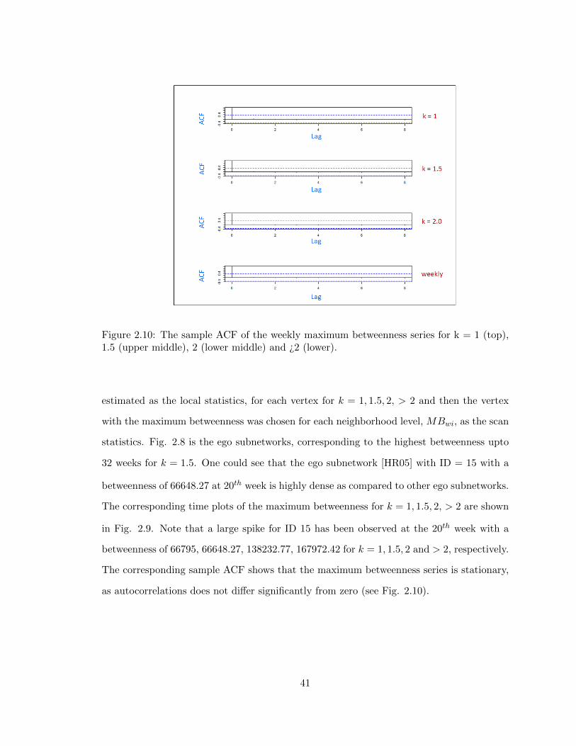
Figure 2.10: The sample ACF of the weekly maximum betweenness series for k = 1 (top),1.5 (upper middle), 2 (lower middle) and ¿2 (lower).
estimated as the local statistics, for each vertex for k = 1, 1.5, 2, > 2 and then the vertex
with the maximum betweenness was chosen for each neighborhood level, MBwi, as the scan
statistics. Fig. 2.8 is the ego subnetworks, corresponding to the highest betweenness upto
32 weeks for k = 1.5. One could see that the ego subnetwork [HR05] with ID = 15 with a
betweenness of 66648.27 at 20th week is highly dense as compared to other ego subnetworks.
The corresponding time plots of the maximum betweenness for k = 1, 1.5, 2, > 2 are shown
in Fig. 2.9. Note that a large spike for ID 15 has been observed at the 20th week with a
betweenness of 66795, 66648.27, 138232.77, 167972.42 for k = 1, 1.5, 2 and > 2, respectively.
The corresponding sample ACF shows that the maximum betweenness series is stationary,
as autocorrelations does not differ significantly from zero (see Fig. 2.10).
41

2.5.3 Estimation of LLR Using Binomial Model
As the betweenness is proportional to the number of geodesic distances around a vertex
and therefore, it can be modeled as Binomial distribution. Under the null hypothesis,
observations, x1, x2, ..., xN are from an i.i.d Binomial distribution with success probability
p0. For alternative hypothesis, there would be a scanning window of width, w, where
observations are from an i.i.d Binomial distribution with different success probability p1,
and the observations in the rest of the intervals, [1, t) and [t+w, N ], are from an i.i.d
Binomial distribution with success probability p0. Here Xi = the number of shortest paths
in the neighborhood such that:
Xi =
(ni − 1)(ni − 2), for directed graph,
(ni−1)(ni−2)2 , for undirected graph.
For variable and overlapping windows, p0 and p1 can be estimated from the data as p0 =
∑ti=1 xi∑ti=1Xi
and p1 =∑ti=s xi∑ti=sXi
[PS00], where xi = the number of shortest paths that is traversed
by the vertex, i, in the neighborhood. The null hypothesis is H0 : p0 = p1, and the
alternative hypothesis is H1 : p1 > p0. The likelihood under the null hypothesis is:
LH0 =
N∏i=1
(Xi
xi
)pxi0 (1− p0)Xi−xi . (2.12)
The likelihood under the alternate hypothesis is:
LH1 =
(m−1∏i=1
(Xi
xi
)pxi0 (1− p0)Xi−xi
)×
(t∏
i=m
(Xi
xi
)pxi1 (1− p1)Xi−xi
)
×
(N∏
i=t+1
(Xi
xi
)pxi0 (1− p0)Xi−xi
).
(2.13)
42

The likelihood ratio, Λ, chosen as test statistic, is given by:
Λ =Likelihood under H1
Likelihood under H0=
(∏ti=m
(Xixi
)pxi1 (1− p1)Xi−xi
)(∏t
i=m
(Xixi
)pxi0 (1− p0)Xi−xi
) . (2.14)
Therefore, the LLR can be written as:
log(Λ) =∑t
i=m[xi log(p1p0 ) + (Xi − xi) log (1−p1)(1−p0) ]
= a1Nt + a2(∑t
i=mXi −Nt),
(2.15)
where a1 = log(p1p0
), a2 = log (1−p1)
(1−p0) and Nt =∑t
i=s xi. Using equation 2.1, one could write
for rejecting H0:
max (log(Λ)) ≈ Sw. (2.16)
Fig. 2.11 shows the estimated value of the LLR as a function of m. It is observed
that the maximum LLR and the second maximum LLR for k = 1.5, 2.0, ≥ 2 occur in the
20th week (the 4th week of October 2003) and at the 21st week (the first week of November
2003), respectively. The associated ego subgraphs corresponding to the largest LLR and the
second largest LLR are shown in Fig. 2.12, showing individuals with ID = 15 and 5 have the
highest and the second highest betweenness, respectively. The largest LLR and the second
largest LLR for k = 1.5, 2.0, > 2.0 are given in Table 2.3. All these estimated LLR values are
greater than the critical values and therefore, statistically significant. Therefore, the clusters
of shortest paths traversed by the vertices with ID = 15 (see Fig. 2.13)and 5 at the 20th
and the 21st week, respectively, in the neighborhood are statistically significant, suggesting
that excessive communications have been transmitted through these two individuals.
43

Figure 2.11: The estimated LLR as a function of variable and overlapping w for k = 1.5(toppanel), 2(middle panel), > 2 (lower panel) for the 32 week period in 2003 around the primarycluster.
Table 2.3: The maximum log likelihood ratio at week 20 and week 21 respectively withGumbel critical values (GCV), standard Monte critical values (SMCV), and significancelevel (SL) for k = 1.5, 2.0 and > 2.0 using the Binomial model.
K LLR: x[20] LLR: x[21] GCV(SL) SMCV(SL)]
1.5 644.11 601.069 7.73 (0.0001) 8.47 (0.001)
2.0 602.74 599.95 7.60 (0.0001) 8.51 (0.001)
> 2 2583.92 2529.41 9.00 (0.0001) 8.50 (0.001)
44

Figure 2.12: The anomalous ego sub network with ID = 15 (upper panel) detected at weekt = 20 in 2003 for k = 1.5 (top left), k = 2(middle) and k = > 2 (top right). The vertexhas maximum absolute betweenness score. Neighborhood ego sub networks with the secondmaximum absolute betweenness score (lower panel) for ID = 5.
2.5.4 Maximum Likelihood Estimation Using Non-Parametric Model
Here a nonparametric method of obtaining an estimate of the maximum likelihood of a
unimodal density has been briefly discussed. This is initially reported for the continuous
case by Robertson [Rob67], when mode is known. This method has later been extended by
Wegman [Weg70], when the mode is unknown. He presented this estimate as conditional
expectation given a Σ-lattice, (E(f |ΣL)). Wegman [Weg70] showed that the MLE must
contain the mode located at one of the observations. However, the MLE that is used as the
unimodal estimator with the largest likelihood product, is not computationally very efficient
as the mode has been estimated for each observation to calculate the likelihood product.
In order to enhance the computational efficiency, Wegman [Weg11] later suggested placing
the mode at the smallest as well as the largest order statistic. In fact, he observed that if
the mode were set at the smallest order statistic, the left-hand side of the density estimate
45

Figure 2.13: Circular plot showing ID = 15 associated with the maximum betweenness inthe middle.
would be flat and the right-hand side would be non-increasing and similarly, if the mode
were placed at the largest order statistic, the right-hand side would be flat and the left-hand
side would be non-decreasing. Thus, the MLE would set the mode between the two flat
regions/bounds. Let x1 ≤ x2 ≤ .... ≤ xn is the ordered sample drawn from a unimodal
density f and L and R be the left and right bounds such that ς = [L, R] = R - L = ε . Let
xl and xr be the largest observation ≤ L and the smallest observation ≥ R, respectively,
and h be any estimate, where [L, R] is the modal interval such that:
E(f |ΣL) =
h(xl), xl < x < L,
h(xr), R < x < xr,
h(x), otherwise.
46

Figure 2.14: (a) The estimated pmf of the maximum betweenness as a function of orderedobservations. (b) The estimated density with mode placed at the smallest order statistic.(c) The estimated density with mode placed at the largest order statistic.
Here this model was applied to estimate MLE for the unimodal discrete case. The raw
probability mass function of the maximum betweenness, f(xi), such that f(xi) =(Xixi
)pxi(1−
p)Xi−xi was initially estimated. The likelihood for each conditional mass function is written
as:
Lj(p) =32∏i=1
fj(x(i)|p), j = 1, 2, ...8. (2.17)
Fig. 2.14(a) shows the raw estimate of the unimodal probability mass function (pmf) for
the maximum betweenness. At first, the mode was placed at the smallest order statistic in
the data sample of the maximum betweenness, which shows a flat region on the left hand
side, and the non increasing region at the right (see Fig. 2.14(b)). Similarly, the mode has
been placed at the largest order statistics (see Fig. 2.14 (c)) to obtain the flat region at
the right, while the non-increasing region can be seen in the left. The left (L) and right
47

Figure 2.15: The Log likelihood estimate using a non-parametric method as a function ofmode.
bounds (R) are x[19] and x[26], respectively. Therefore, the estimated modal interval is [19,
26]. The log likelihood estimate between two bounds as a function of mode is shown in Fig.
2.15. In fact, the MLE is associated with mode at x[20] = 724.18 at week 20 (the 4th week
of October 2003) and the second most likely mode is x[21] = 724.16 (see Fig. 2.15 ) at week
21 (the first week of November 2003). One could see that these results are consistent with
the results obtained from the parametric method.
2.6 Monte Carlo Simulation
Monte Carlo procedure is a very important method to estimate the P values. Here are the
three reasons why this procedure is useful [NCS02].
1. Some test statistics do not have an exact sampling distribution.
2. Despite that a test statistic has an exact distribution, it may not be appropriate for
48

an inadequate sample size.
3. Estimation of exact sampling distribution may be computationally intensive.
This procedure has some limitations. To obtain p-value precision, the number of simu-
lation needs to be increased, which is computationally intensive. On the other hand, Monte
Carlo technique requires no assumption of sampling distribution of the test statistic and
calculates an approximate P value. In the present work, the exact sampling distribution
is not known for most cases, as the anomaly splits among multiple windows, resulting in
overlapping windows and nonrandom clusters.
Let Z be the test statistic having the sampling distribution g under the null hypothesis
and z be its observed value from the data then p value = PH0(Z ≥ z) [CH74b]. The p value
can be estimated as:
p =r
n, (2.18)
where r = (i : zi ≥ z) = number of test statistic from the simulation that is greater than or
equal to the observed test statistic given that n is the simulated replicates and z1, z2, .., zn
are the test statistics from these simulation. However, this p value estimate is not strictly
correct. The unbiased estimate of the true p value is given by [DH97]
p =(r + 1)
(n+ 1). (2.19)
The equation 2.19 can be derived as follows. Let Y be the random variable that denotes
the number that test statistic Z ≥ z. Here the model is:
Y |p ≈ Binomial(n, p), (2.20)
where p ≈ unif(0, 1). The probability that the test statistic Z is greater than or equal to
49

the size z in exactly r simulations is given by [NCS02]:
p(Y = r) =
∫ 1
0p(Y |p)f(p)dp =
(n
r
)∫ 1
0pr(1− p)n−rdp
=
(n
r
)Beta(r + 1, n− r + 1) =
n!
(n+ 1)n!=
1
n+ 1, (2.21)
where Beta(r + 1, n − r + 1) = Γ(r+1)Γ(n−r+1)Γ(n+2) = r!(n−r)!
(n+1)! . The probability that the test
statistic exceeds r or greater in n simulated replicates = p(Y ≥ r) = r+1n+1 .
2.6.1 Evaluation of Performance of Scan Statistic Model
The Monte Carlo simulation was used to evaluate the performance of the hypothesis test in
detecting the primary cluster of events. The power of the scan statistic is the probability
that the observed scan statistic exceeds the critical value k when the alternative hypothesis
is true. For the discrete scan statistic case, the power is written as [GNW01]
P (Sw ≥ k|HA), (2.22)
where Sw(w) = max Yt(w), and Yt(w) is the number of events in in the scanning window w.
The measured responses are the size (α) and the power of the test statistic, log likelihood
ratio. The factors are test statistic, sample size and λ. Here n = 200, 500 and 1000
replications were used for the simulations. The type-I error rate (size) is measured using
the proportion of the times the null hypothesis is rejected out of n replications when the
null hypothesus is true and can be mathematically written as [MM16].
α =1
n
n∑i=1
δi, (2.23)
50

Figure 2.16: The estimated power for the Log likelihood ratio as a function of λ.
where
δi =
1, type-I error,
0, no type-I error.
The simulated sizes and the critical values (CV) are presented in Tables 2.4 and 2.5, respec-
tively. It was observed that the size distortion for the test statistic improves as the sample
size increases. The sizes are quite closer to the nominal level when n = 500 and 1000.
For measuring the power, the probability of making type-II error (β), which is the
proportion of the times the null hypothesis is not rejected out of n replications when the
alternative hypothesis is true, has been estimated and can be mathematically expressed as
[MM16]:
β =1
n
n∑i=1
ζi, (2.24)
51
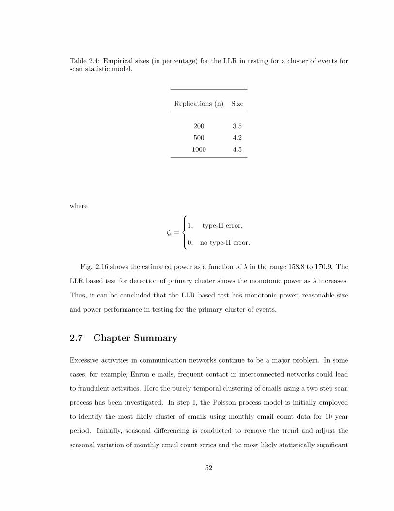
Table 2.4: Empirical sizes (in percentage) for the LLR in testing for a cluster of events forscan statistic model.
Replications (n) Size
200 3.5
500 4.2
1000 4.5
where
ζi =
1, type-II error,
0, no type-II error.
Fig. 2.16 shows the estimated power as a function of λ in the range 158.8 to 170.9. The
LLR based test for detection of primary cluster shows the monotonic power as λ increases.
Thus, it can be concluded that the LLR based test has monotonic power, reasonable size
and power performance in testing for the primary cluster of events.
2.7 Chapter Summary
Excessive activities in communication networks continue to be a major problem. In some
cases, for example, Enron e-mails, frequent contact in interconnected networks could lead
to fraudulent activities. Here the purely temporal clustering of emails using a two-step scan
process has been investigated. In step I, the Poisson process model is initially employed
to identify the most likely cluster of emails using monthly email count data for 10 year
period. Initially, seasonal differencing is conducted to remove the trend and adjust the
seasonal variation of monthly email count series and the most likely statistically significant
52

Table 2.5: The simulated critical values for the LLR for n = 1000.
(1- α) % value
90 1.349809
95 1.916925
97.5 2.70383
99 3.353406
99.5 4.547692
temporal primary cluster is detected using the maximum LLR as the scan statistic (LLR
= 82.07, p = 0.001). In step II, the binomial model is applied to weekly network data of
emails for the 32 week period in 2003 in the neighborhood of the most likely cluster, where
betweenness is implemented as the locality statistics and the most likely purely temporal
clusters of emails are observed for k = 1.5, 2 and > 2 using the maximum LLR as the scan
statistic. The two-step scan statistic process modeling to estimate the excessive activities
as well as identifying most important nodes/vertices here for the large data set would be
more scalable or computationally less intensive, as the most likely cluster in the entire data
set was first identified using count data, and then the network was extracted in the vicinity
of the primary cluster.
53

Chapter 3: Anomaly Detection Using Univariate and
Multivariate Time Series Models
3.1 Introduction
In the previous chapter, the existence of significant excessive activities in the e-mail networks
has been demonstrated using scan statistics. It is not apparent from the study the dynamic
relationship between the influential vertices or nodes associated with excessive activities in
the e-mail network. As the scan statistics measure the maximum of locality statistics, it
can conceal the group of influential people in the network. In this chapter, two alternative
approaches to detect clusters in a point process are implemented using the graph edit
distance (GED).
Initially, the univariate time series of the GED between subsequent weekly subgraphs
has been constructed and then fitted the time series to the auto regressive moving average
(ARMA) model. The anomalies were then assessed using the residual thresholds obtained
from the fitted time series model. Additionally, this chapter considers multiple time series
of neighborhood ego subnetworks using the GED. A vector auto regressive (VAR) model
was applied to fit the multiple time series. The VAR model has previously been used in
economics and finance, accounting and marketing [Sim80]. In economics, this model is
applied to forecast and predict macroeconomic variables, such as gross domestic product
(GDP), money supply and unemployment. Here the VAR model has been implemented on
time series of ego subgraphs in e-mail networks to investigate the excessive activities, as the
nodes or vertices of the subgraphs are interrelated or cross correlated. Using this model,
the dynamic relationship between vertices, and the excessive activities associated a vertex
or node can be obtained. In addition, the group of influential persons (IDs) or vertices or
nodes in the e-mail subnetworks can be identified using this process.
54

3.2 Univariate Time Series from e-mail Networks
3.2.1 Graph Distance Metrics
Several graph distance metrics, such as maximum common subgraph (MCS) edge distance,
MCS vertex distance, graph edit distance (GED), modality distance (MD), diameter dis-
tance (DD)and spectral distance (SD) can be used to form univariate time series. Here we
mostly use GED, d(G,H), which is a measure of similarity (or dissimilarity) between two
graphs, G and H. The GED can be defined as [Pin05]:
d(G,H) = |VG|+|VH |−2|VG ∩ VH |+|EG|+|EH |−2|EG ∩ EH |, (3.1)
where EG and VG are the edge set and vertex set of a graph, G, respectively, and EH and
VH are the edge set and vertex set of a graph, H, respectively [Pin05], [?]. The union of
two graphs G(VG, EG) and H(VH , EH) are the union of their vertex sets and edge sets. It
can be expressed as:
G ∪H = (VG ∪ VH , EG ∪ EH) . (3.2)
Similarly, the intersection of two graphs, G(VG, EG) and H(VH , EH), is the union of their
vertex sets and the intersection of their edge sets. It can be written as:
G ∩H = (VG ∪ VH , EG ∩ EH) . (3.3)
3.2.2 Graph Edit Distance to Time Series
The GED between the weekly networks, as shown in Fig. 3.1, was obtained using Eq. 3.1.
The distances between the networks for four weeks are given in Table 3.1. Fig. 3.2(a) shows
the time plot of observed graph edit distance for 52 weeks around the most likely cluster
obtained from scan statistics in Chapter 1. One could observe a spike at around week 20
(the 4th week of October 2003) and at week 21 (the first week of November 2003). The
55

Figure 3.1: Weekly subnetworks at different time points. The GED was estimated fromadjacent periods to compare subgraphs sequentially.
sample ACF and PACF show that the series is stationary (see Fig. 3.2(b)). To further
validate this point, the unit root tests, such as augmented Dickey-Fuller, Phillips-Perron
[CM09], [Pfa08] and KPSS [Pfa08] tests were performed to show that the time series is
stationary. The values of the test statistics, lag parameters and the corresponding p-values
are given in Table 3.2. A time series model was then fitted to the graph distance time series,
as shown in Fig. 3.2(a) to get the residual. Here three time series models, ARMA, AR and
MA are discussed.
3.2.3 AR model
The autoregressive (AR) model of order p with no constant term can be written as [SS06]:
xt = φ1xt−1 + φ2xt−2 + ....+ φpxt−p + wt, (3.4)
56

Figure 3.2: (a)Time Plots of observed and fitted GED series using ARMA Model for the52 week period June 2003 - June 2004. (b) The sample ACF (top panel) and the samplePACF (lower panel) of weekly GED series for the 52 week period June 2003 - June 2004,respectively.
Table 3.1: The order of a graph G, the order of graph H, the size of graph G, size of a graphH, and the graph edit distance between two graphs, G and H.
|VG| |VH | |EG| |EH | d(G,H)
w1-w2 73 38 93 55 73
w2-w3 38 39 55 41 15
w3-w4 39 76 41 168 164
where xt is stationary, φ1, φ2, ..., φp are parameters and φp 6= 0. Here wt is the white noise
with mean zero and variance σ2w. The AR (p) model is also given in useful form using
57

Table 3.2: Tests for unit roots showing that the time series is stationary.
Unit root test Value of test statistics Lag Parameter p-value
Augmented Dickey-Fuller Test -4.72 1 0.01
Phillips-Perron Test -4.18 3 0.01
KPSS Test 0.145 1 0.1
backshift operator, B, as
(1− φ1B − φ2B2 − ...− φpBp)xt = wt,
φ(B)xt = wt,
(3.5)
where Bxt = xt−1 and φ(B) = 1 − φ1B − φ2B2 + ... − φqBq, and φ(B) is called an auto
regressive operator.
3.2.4 MA model
The moving average (MA) model with no constant term of order q can be written as [SS06]:
xt = wt + θ1wt−1 + θ2wt−2 + ...+ θqwt−q, (3.6)
where θ1, θ2, ..., θq are parameters and θq 6= 0. Using backshift operator, B, the model is
written as
xt = θ(B)wt, (3.7)
where θ(B) = 1 + θ1B + θ2B2 + ...+ θqB
q, and θ(B) is called a moving average operator.
58

3.2.5 ARMA model
The ARMA (p, q) models with no constant term are well-known statistical models for a
stationary time series xt and can be mathematically expressed as [SS06]:
xt = φ1xt−1 + ...+ φpxt−p + wt + θ1wt−1 + ...+ θqwt−q,
(1− φ1B − φ2B2 − ...− φpBp)xt = (1 + θ1B + θ2B
2 + ...+ θqBq)wt,
φ(B)xt = θ(B)wt,
(3.8)
where wt ∼ iid N(0, σ2w) and (φ1, ..., φp, θ1, ..., θq) is a (p + q) × 1 vector of parameters,
such that φp 6= 0, θq 6= 0 and σ2w > 0, and p, q are the orders of the autoregressive part
and the moving average part of the model, respectively. Here xt is the current value of the
time series, which is a linear function of past values of the time series and past values of the
errors. In fact, xt can be expressed as a function of autoregressive part and moving average
parts. The anomalies were then assessed using the residual threshold obtained from the
model fitted to the time series.
3.3 Estimation of Parameters
3.3.1 Maximum Likelihood for ARMA(p,q) Process
The likelihood function is given by [SS06]:
L(φ1, ....φp, θ1....θq, σ2w) =
∏nt=1 f(xt|xt−1, ..., x1)
=
exp
−∑nt=1
[xt−x
t−1t (β)
]22σ2wr
t−1t (β)
(2πσ2
w)n2 [(r01(β),r12(β),...,rn−1
n (β)]12,
(3.9)
59

where β = (φ1, ...φp, θ1, ..., θq)′ and xt|xt−1, ..., x1 ∼ N(xt−1
t , P t−1t ), the conditional vari-
ance, P t−1t = σ2
wrt−1t and the mean, xt−1
t = E(xt|xt−1, ..., x1). The logarithm of likelihood
function is given by:
l(β, σ2w) = logL(β, σ2
w)
= −n2 log(2πσ2
w)− 12
[log r0
1(β) + log r21(β).....+ log rn−1
n (β)]−
∑nt=1[xt−x
t−1t (β)]
2
2σ2wr
t−1t (β)
.
(3.10)
Taking the partial derivative with respect to σ2w one can obtain
∂l
∂σ2= − n
2σ2w
+
∑nt=1
[xt − xt−1
t (β)]2
2σ4wr
t−1t (β)
= 0, (3.11)
σ2w = n−1
∑nt=1
[xt − xt−1
t (β)]2
rt−1t (β)
. (3.12)
Newton-Raphson algorithm is a powerful numerical optimization technique for the maxi-
mum likelihood estimation of β. Let β = (β1, ......., βk) denote k parameters. The necessary
condition for maximizing l(β) is:
∂l(β)
∂βj= 0, j = 1, ..., k. (3.13)
The k × 1 vector of partials is given by:
l(1)(β) =
(∂l(β)
∂β1, ....,
∂l(β)
∂βk
)′. (3.14)
60

Similarly, the k × k matrix of the second order partials can be written as:
l(2)(β) =
(∂l2(β)
∂βi∂βj
)ki,j=1
, (3.15)
assuming l2(β) is nonsingular. If β(0) is the initial estimate of β, then using the Taylor
expansion, one gets the following expressions:
0 = l(1)(β) ≈ l(1)(β(0))− l(2)(β(0))[β − β(0)], (3.16)
β(1) = β(0) + [l(2)(β(0))]−1l(1)(β(0)). (3.17)
Here β(2) is obtained by replacing of β(0) by β(1), and so on. The iteration has been carried
out until the sequence of estimators, β(1), β(2), ..., would converge to β, the MLE of β.
3.3.2 Yule-Walker Estimation for an AR(p) Process
One of the commonly used methods to estimate the AR(p) model parameters is Yule-Walker
estimation. If xt be an autoregressive stochastic process of order p then;
xt = φ1xt−1 + .....+ φpxt−p + wt. (3.18)
Multiplying Eq. 3.18 by xt−h and taking expectation gives the set of equations, known as
the Yule-Walker equation [SS06],
E[xt−hxt] = E[φ1xt−1xt−h + .....+ φpxt−pxt−h + wtxt−h],
γ(h) = φ1γ(h− 1) + .....+ φpγ(h− p), h = 1, 2, ..p,
(3.19)
σ2w = γ(0)− φ1γ(1)− ...− φpγ(p), h = 0. (3.20)
61

In matrix notation,
Γpφ = γp, (3.21)
σ2w = γ(0)− φ′γp. (3.22)
Γp =
γ(0) γ(1) ... γ(p− 1)
γ(1) γ(0) ... γ(p− 2)
.
.
.
γ(p− 1) γ(p− 2)...γ(0)
, φ =
φ1
φ2
.
.
.
φp
, γp =
γ(1)
.
.
.
.
γ(p)
, (3.23)
where Γp is (p× p) covariance matrix, and φ and γp are (p× 1) vectors. Using the method
of moments, in Eq. 3.21, replacing γ(h) by γ(h), one can get
φ = Γ−1p γp, σ2
w = γ(0)− γ ′pΓ−1p γp. (3.24)
These estimators are called the Yule-Walker estimators. In terms of sample ACF, one can
write the Yule-Walker estimators as
φ = R−1p ρp, σ2
w = γ(0)[1− ρ′pR−1
p ρp
], (3.25)
62

where ρp is a (p× 1) vector, and Rp, a (p× p) matrix, is written as:
Rp =
1 ρ(1) ... ρ(p− 1)
ρ(1) 1 ... ρ(p− 2)
.
.
.
ρ(p− 1) ρ(p− 2)... 1
. (3.26)
3.3.3 Estimation Method for MA(1) Process
If xt is a moving average stochastic process of order 1, then
Xt = wt + θwt−1, |θ|< 1. (3.27)
Multiplying both sides by Xt−h and taking expectation, one gets E[XtXt−h] = E[wtXt−h+
θwt−1Xt−h]. For h = 0, the population autocovariance is γ(0) = σ2w(1 + θ2). For h = 1,
γ(1) = σ2wθ, and the estimate of θ can be obtained by solving [SS06]
ρ(1) =γ(1)
γ(0)=
θ
1 + θ2. (3.28)
If |ρ(1)|≤ 12 , the solutions are real. When |ρ(1)|< 1
2 , the estimate is
θ =1−√
1−4ρ(1)2
2ρ(1) ,
σ2w = γ(0)
1+θ2.
(3.29)
63

Table 3.3: The estimated parameters and AIC of ARMA models.
Parameter ARIMA(0,0,1) SE ARIMA(2,0,0) SE ARIMA(1,0,1) SE
ar1 0.5470 0.1336 -0.0412 0.2417
ma1 0.611 0.1198 0.6394 0.1963
ar2 -0.2617 0.1325
AIC 685.147 688.343 687.1195
Figure 3.3: The standardized residual series (upper panel) for the MA(1)fit to the GEDseries and the ACF of standardized residuals for the MA(1) fit to the GED series (middlepanel), and p-values for the Ljung-Box-Pierce Q-statistic (lower panel for the MA(1) fit tothe GED series).
64

3.4 Excessive Activities and Residuals
The residual, et and the standardized residuals, set, are mathematically expressed as [SS06]
et = xt − xtt−1,
set = (xt−xtt−1)√P t−1t
,
(3.30)
where xtt−1 is the one-step-ahead prediction of xt and P t−1
t is the estimated one-step-ahead
error variance. The residual has some properties with mean = 0 and constant variance,
i.e. homoscedasticity and normally distributed. As it is normally distributed, the 95% of
all values fall between twice the standard error. Therefore, the observations lying beyond
twice the standard deviations were identified as anomalies.
The augmented Dickey-Fuller test [CM09], Phillips-Perron test [CM09] and KPSS [Pfa08]
test have been applied to the time series of the observed graph edit distance for 52 weeks
around the most likely communication clusters obtained from the scan statistics with a spike
at around week 20 (the 4th week of October 2003) and week 21 (the first week of November
2003) to show that the time series is stationary. The distinct cutoff of the sample ACF
at lag1 combined with tailing off of the sample PACF suggests an MA(1) would be an
appropriate fitted model to the data [CM09]. Alternatively, the tailing off of the sample
ACF and the distinct cutoff of the sample PACF suggests the AR(2) model.
The MA(1), AR(2), ARMA(1,1), ARMA(2,1) models have been fitted to the time series
of GED. The optimal model is obtained based on the Akaike’s information criterion (AIC)
and the optimal model is an MA(1) that minimizes the AIC, followed by the ARMA(1,1),the
AR(2)(see Table 3.3). The time plot of the standardized residuals (below) shows variance
remains nearly constant except one observation that lies beyond the six times standard
deviations (see Fig. 3.3).
The Ljung-Box-Pierce Q-statistic [SS06] is Q = n(n + 2)∑H
h=1ρ2r(h)n−h , where ρr(h) is
the sample autocorrelations of the residuals. The Q-test has been applied on the residuals
65

Figure 3.4: The histogram of the residuals (upper panel) and the Normal Q-Q plot of theresiduals of the MA(1) fit to the GED series (lower panel), showing the residuals are closeto normality except for an extreme value in the right tail.
obtained from the fitted model to check serial correlations of the residuals[Che02]. The null
hypothesis for the first H autocorrelations is H0 : ρr(1) = ρr(2) = ... = ρr(H) = 0, and the
alternative hypothesis is H1 : ρr(h) 6= 0 for some h = 1, 2, ...,H. Under the null hypothesis,
the asymptotic distribution of Q is Q ∼ χ2H−p−q, where H is the number of lags. The sample
auto correlation function (ACF) of standardized residual and the Q-statistic show that the
residuals are random (see Fig. 3.3). One could see from the histogram and the normal Q-Q
plot of residuals that the residuals are approximately normal except for an extreme value
in the right tail (see Fig. 3.4). Therefore, from these analyses, it can be concluded that the
spike at week 20 in the GED series is associated with excessive activities.
66

Figure 3.5: The neighborhood ego networks for k = 1 for ID = 5 for the 52 week period,June 2003 - June 2004.
3.5 Graph Edit Distance to Multiple Time Series
Multivariate time series is a very useful technique in time series analysis and can be used
when one wants to regress a stationary time series in terms of its own past values and
past values of other stationary time series. The communications in the e-mail networks
are interrelated. As a result, these dynamic relationships in the email networks among IDs
cannot be modeled by the univariate time series. To overcome this, the vector autoregression
process has been employed to model the dynamic relationship between different IDs (nodes)
that are associated with the excessive communication, and detect the chatter.
Initially, the data set, X, is partitioned around the most likely cluster obtained from the
two-step scan process for 52 weeks into n disjoint weekly subintervals, wi, i = 1, 2, ..., n such
that Xi ∈ wi. A family of neighborhood ego subnetworks has been generated for different
IDs in the email networks for different neighborhood levels, k = 1, 1.5 and 2. Figs. 3.5 and
3.6 show the ego subnetworks of ID = 5 for 52 weeks for k = 1 and k = 1.5, respectively.
67

Figure 3.6: The neighborhood ego networks for k = 1.5 for ID = 5 for the 52 week period,June 2003 - June 2004 around the primary cluster estimated from monthly temporal scanstatistic model.
The distance metric, GED, was then estimated to quantify the difference between the two
consecutive ego subnetworks for k = 1, 1.5 and 2 to construct the multiple time series for
different IDs.
In the data set, it has been observed that a number of participants have high missing
values. Note that in chapter 2, the ID = 15 has been identified as the most influential person
at week 20 (4th week of October 2003) using the scan statistic model. It has been observed
that this individual (ID = 15) has missing values of 90% in the time series, suggesting that
the individual may not be the most influential person in the network. This node (ID = 15)
in the email network might be simply a connector or a hub in the email network and might
not play a vital role in the network. In this research work, five individuals, IDs = 1, 5, 7,
10 and 20, with missing values between 5 to 15 % have been considered to construct the
multiple time series of GED. Hence, a five-dimensional GED series has been generated.
Handling missing values is an important step in statistical analysis.In time series, the
68

Figure 3.7: (a) Weekly GED series estimated from adjacent periods to compare subgraphssequentially with missing values for ID = 1. Weekly GED series for ID = 1 (lower panel)after the imputation of missing values with mean. (b) The time plots of GED with differentimputation methods for ID = 1.
well-known imputation algorithms are based on multiple imputation [Rub87], expectation
maximization [DLR77] and nearest neighbors [VA80]. A variety of different imputation
algorithms, such as imputation by mean, median and mode, imputation by linear inter-
polation, spline interpolation and Stineman interpolation, imputation by structural model
and Kalman smoothing, and imputation by seasonally decomposed (seadec) missing values
exist in the literature to handle the missing values in the time series [MBB17]. Figs. 3.7
(a) shows the time plots with missing values (upper panel) and the corresponding time
plots with imputed values using mean (lower panel). Time series with the other imputation
methods, such as median, interpolation, Kalman and seadec is shown for comparison (see
Fig. 3.7(b)). Note that most of the algorithms give similar results. Here the mean impu-
tation to handle time series missing values has been considered, as the time series does not
show any trend and seasonality.
69

Figure 3.8: (a) A five-dimensional GED series for IDs = 1, 5, 7, 10 and 20 for k = 1.0. Notethe spike at week = 20 for ID = 5. (b) The univariate GED series plotted separately forthese IDs.
The GED between the ego subnetworks for ID = 1, 5, 7, 10 and 15 was obtained using
Eq. 3.1. Figs., 3.8, 3.9 and 3.10 show the time plots of the observed graph edit distance for
52 weeks for k = 1, 1.5 and 2, respectively. One could see that the ego subnetworks show
a large spike in the GED for ID = 5 for k = 1.0 and all the IDs for k = 2 at week 20. To
implement the VAR model, the first step is to select the variables, and then investigate the
stationarity of the time series. The next step is to determine the order of the VAR model,
and to fit the model, and finally to perform the model checking using the residual analysis
[Tsa14].
3.6 Variable Selection of the VAR model
To select the variables, the correlation between the variables need to be determined. Here
the nodes with ID = 1, 5, 7, 10, and 20 have been selected for the multivariate analysis, and
70

Figure 3.9: (a) A five-dimensional GED series for IDs = 1, 5, 7, 10 and 20 for k = 1.5. Notethe spike at week = 20 for IDs = 5 and 7. (b) The univariate GED series plotted separatelyfor these IDs.
the correlations among IDs have been checked using correlation bar plots, scatter plot matrix
and parallel coordinate plots. The correlation bar plots show the correlation magnitude of
the IDs increases with k (see Fig. 3.11). The different IDs are mostly positively correlated
for k = 2. The correlation strength is more than 75 % for k = 2 for all variables. A similar
trend for k = 2 can also be observed in scatter plot matrices of different variables, as shown
in Fig. 3.12. For k = 1 and 1.5, IDs are observed to be correlated to some extent.
To extract interesting data structures, the parallel coordinate plot, which is an efficient
way to represent multidimensional data, has been employed. The interesting data struc-
tures, such as the two-dimensional features (correlation and nonlinear structures) [Weg90]
can be observed. Here the graph edit distances of IDs = 20, 10, 7, 5 and 1 are plotted in
parallel fashion in two dimensions (see 3.13) for k = 2. One could see the crossing between
ID 10 and ID 20 for k = 1, 1.5, 2, suggesting a little negative correlation whereas an approx-
imate parallelism and relatively fewer crossings exists between the variables, suggesting a
71

Figure 3.10: (a) A five-dimensional GED series for IDs = 1,5, 7, 10 and 20 for k = 2.0.Note the spike at week = 20 for IDs = 5 and 7. (b) The univariate GED series plottedseparately for these IDs.
positive correlation for k = 2 [Weg90], [GW16]. Also, one can observe the negative slope
connecting the low GED of ID 7 and ID 5 to moderate to high GED of ID 5 and ID 1,
respectively, which suggests the presence of an outlier. The other interesting feature is the
separation of observations for variables at high levels that is propagating across the parallel
coordinates for k = 2, suggesting the presence of two clusters that might be associated with
the excessive activities.
3.7 Vector Autoregressive Model
Let Yt = (y1,t, y2,t, ..., yn,t) be a n-dimensional multiple time series for t = 1, 2, ..., T , where
T is the sample size of each time series with the same sample period. The first-order vector
72

Figure 3.11: (a,b,c) Correlation bar plots of the GED for ID = 1, 5, 7, 10 and 20 withk = 1, 1.5 and 2, respectively.
autoregression model, VAR(1), is defined as [ZW06]:
y1,t = α1 + φ11y1,t−1 + φ12y2,t−1 + ...+ φ1nyn,t−1 + w1,t
y2,t = α2 + φ21y1,t−1 + φ22y2,t−1 + ...+ φ2nyn,t−1 + w2,t
.
.
yn,t = αn + φn1y1,t−1 + φn2y2,t−1 + ...+ φnnyn,t−1 + wn,t.
(3.31)
73

Figure 3.12: A scatterplot matrix of five-dimensional GED data illustrating correlations fork = 2.
The vector autoregression model of order p, VAR(p), can therefore be written as [ZW06]:
y1,t = α1 + φ111y1,t−1 + φ1
12y2,t−1 + ...+ φ11nyn,t−1 + φ2
11y1,t−2 + φ212y2,t−2+
...+ φ21nyn,t−2 + ...+ φp11y1,t−p + φp12Y2,t−p + ...+ φp1nyn,t−p + w1,t
y2,t = α2 + φ121y1,t−1 + φ1
22y2,t−1 + ...+ φ12nyn,t−1 + φ2
21y1,t−2 + φ222y2,t−2+
...+ φ22nyn,t−2 + ...+ φp21y1,t−p + φp22y2,t−p + + φp2nyn,t−p + w2,t
.
.
yn,t = αn + φ1n1y1,t−1 + φ1
n2y2,t−1 + ...+ φ1nnyn,t−1 + φ2
n1y1,t−2 + φ2n2y2,t−2
+...+ φ2nnyn,t−2 + ...+ φpn1y1,t−p + φpn2y2,t−p + + φpnnyn,t−p + wn,t.
(3.32)
74

Figure 3.13: (a,b,c) Parallel coordinate plot of five-dimensional GED data showing correla-tions for k = 1, k = 1.5, and k = 2 respectively.
In matrix notations, VAR(p) can be written as:
y1,t
y2,t
.
.
.
yn,t
=
α1
α2
.
.
.
αn
+
φ111 . φ1
1n
φ121 . φ1
2n
. . .
. . .
. . .
φ1n1 . φ1
nn
y1,t−1
y2,t−1
.
.
.
yn,t−1
.+
φp11 φp12 . φp1n
φp21 φp22 . φp2n
. . . .
. . . .
. . . .
φpn1 φpn2 . φpnn
y1,t−p
y2,t−p
.
.
.
yn,t−p
+
w1,t
w2,t
.
.
.
wt,n
.
(3.33)
Similarly, one can write [Lut06]:
Yt = α+ Φ1Yt−1 + Φ2Yt−2 + ...+ ΦpYt−p +Wt. (3.34)
75

Figure 3.14: (a) Weekly GED series for IDs = 1,5, 7, 10 and 20 for k = 1.0 with kernelsmoothing, showing no trend in the kernel fit to the series.
where
Yt =
y1,t
y2,t
.
.
.
yn,t
, α =
α1
α2
.
.
.
αn
, Wt =
w1,t
w2,t
.
.
.
wn,t
(3.35)
76

Figure 3.15: (a) Weekly GED series for IDs = 1, 5, 7, 10 and 20 for k = 2.0 with kernelsmoothing, showing no trend in the kernel fit to the series.
are (n × 1) vectors and Φ1,Φ2...Φp are (n × n) coefficient matrices. Wt is a multivariate
white noise, such that[Pfa08]:
E(Wt) = 0,
E(WtW′τ ) = ΣW , if t = τ,
E(WtW′τ ) = 0, if t 6= τ,
(3.36)
where ΣW is time invariant positive definite covariance matrix.
77

3.7.1 Bivariate VAR(1) Model
The bivariate VAR(1) model is given by [Tsa14]:
y1,t = α1 + φ11y1,t−1 + φ12y2,t−1 + w1,t,
y2,t = α2 + φ21y1,t−1 + φ22y2,t−1 + w2,t.
(3.37)
In matrix notation,
Yt = α+ ΦYt−1 +Wt. (3.38)
Yt =
y1,t
y2,t
, Yt−1 =
y1,t−1
y2,t−1
, α =
α1
α2
, Φ =
φ11 φ12
φ21 φ22
, Wt =
w1,t
w2,t
,(3.39)
such that E(WtW′t) =
σ2w1
σ2w1w2
σ2w1w2
σ2w2
= ΣW and E(WtW′s) =
0 0
0 0
= 0 for t 6= s. In
Eq.(3.41), Φ estimates the dynamic dependence in Y. Here the term, φ12 describes the
linear dependence of y1,t on y2,t−1 in presence of y1,t−1. Similarly, the term, φ21 describes
the linear dependence of y2,t on y1,t−1 in presence of y2,t−1. Here one can consider the
following three cases [Tsa14].
(i) In Φ, if the off diagonal elements, φ12 = φ21 = 0, then Eq. 3.40 reduces to the
following univariate AR(1) model
y1,t = α1 + φ11y1,t−1 + w1,t
y2,t = α2 + φ22y2,t−1 + w2,t.
(3.40)
Note that two series, y1,t and y2,t, are uncoupled and dynamically uncorrelated.
78

(ii) If φ12 = 0, but φ21 6= 0, then we get
y1,t = α1 + φ11y1,t−1 + w1,t
y2,t = α2 + φ21y1,t−1 + φ22y2,t−1 + w2,t.
(3.41)
In this model, note that y1,t does not depend on the past value of y2,t. However y2,t
depends on the past value of y1,t.
(iii) If φ12 6= 0, but φ21 = 0, then we have
y1,t = α1 + φ11y1,t−1 + φ12y2,t−1 + w1,t
y2,t = α2 + φ22y2,t−1 + w2,t.
(3.42)
In this case, note that y1,t depends on the past value of y2,t. However, y2,t does not
depend on the past value of y1,t.
3.8 The Stationarity of Time Series
3.8.1 Stationarity Condition
One can write the bivariate VAR(1) model in companion form without the constant term
as [Pfa08]:
Yt = ΦYt−1 +Wt. (3.43)
The characteristic polynomial of Φ is
det
φ11 φ12
φ21 φ22
− λ1 0
0 1
= det
φ11 − λ φ12
φ21 φ22 − λ
= λ2−(φ11 +φ22)λ+(φ11φ22−φ12φ21).
(3.44)
79

Table 3.4: Roots of the characteristic polynomial for k = 1, 1.5 and 2.
k 1 2 3 4 5
1 0.5664 0.3701 0.2957 0.2957 0.0043451.5 0.6794 0.392 0.392 0.297 0.23182.0 0.5026 0.346 0.346 0.05812 0.05812
Thus, the eigenvalues of Φ are the values of λ such that
det(Φ− λI) = 0. (3.45)
Yt is a stationary process if and only if the eigenvalues of Φ have moduli less than 1
[Pfa08], i.e. the values are within the unit circle. One could observe that the roots of
the characteristic polynomial are less than 1, suggesting that all the variables in the VAR
process are integrated of order 0 ( see Table 3.4).
3.8.2 Stationarity Condition: ADF Tests
The observed GED series of ID1, ID5, ID7, ID10 and ID20 exhibits no increasing or de-
creasing trend with a nonzero mean (see Figs. 3.14 and 3.15). To check the stability of the
GED series for all IDs, the ADF test, which is one of the unit root tests [Bro08], has been
applied. The ADF test regression with constant only (no trend and nonzero mean) can be
written as [NP95]:
∆Yt = α+ ψYt−1 +
p∑j=1
λj∆Yt−j + εt, (3.46)
80

where α is a constant, ∆Yt = Yt − Yt−1 and p is the number of lagged differenced terms.
The test statistic, τ , for the ADF test is defined as [Bro08]:
τ2 =ψ
SE(ψ). (3.47)
The ADF test hypothesis is as follows,
H0 : ψ = 0⇒ Yt ∼ I(1), without drift,
Ha : ψ < 0⇒ Yt ∼ I(0), with nonzero mean,
(3.48)
where the I(1) series has one unit root, and the I(0) series is a stationary process. If a
nonstationary series, Yt, becomes stationary after differencing d times, then the series Yt is
said to be integrated of order d, which can be written as Yt ∼ I(d) and ∆dYt ∼ I(0) [Bro08].
If Xt and Yt are integrated of order 1, then Xt ∼ I(1) and Yt ∼ I(1), suggesting Xt
and Yt are stationary after differencing once. Then these two series, Xt and Yt, are
cointegrated if there exists a such that Xt+aYt is stationary [EG87], [EG87], [BDGH93].
For ADF test, one has to specify the order of the serial correlation (p) or the lag length
of the error term, εt [Sta10]. Ng and Perron [NP95] suggested the data dependent lag length
selection method for ADF test. In fact, it is observed that with this lag length selection the
size of the ADF test is reliable, and the loss of power is minimum [NP01]. The steps for this
selection procedure are [NP95]; (i) Select an upper bound pmax for p. (ii) Then estimate
the ADF test regression with p = pmax (iii) If the absolute value of the t statistic for testing
the significance of the last lagged difference is > 1.6, then the ADF test is performed.
Otherwise, the lag length is reduced by one, and the process is repeated.
For an upper bound pmax for p, Schwert [Sch89] suggested that Pmax = [x], where
x = 12 × ( T100)
14 and [x] is the integer part of x. The pmax = 10 has been estimated for
81

the 5-dimensional GED series. Since the observed processes contain no trend and have
nonzero mean, an ADF regression [Pfa06] with a constant (no trend and nonzero mean)
has been estimated using pmax = 10. Here lag = 1 is selected using the Ng-Perron [NP95]
algorithm. In addition, lag = 1 is obtained by minimizing the AIC. The critical values of
the test statistic, tau2, for the significance levels of 1%, 5%, and 10% [Pfa06] are -3.51, -2.89
and -2.58, respectively. The test statistics and critical values are given in Table 3.5 for the
observed series, ID1, ID5, ID7, ID10, and ID20 for k = 1, 1.5 and 2. It can be concluded
that the observed series, ID1, ID5, ID7, ID10, and ID20 are integrated of order zero or
stationary with a nonzero mean at 5% significance level. In addition, the autocorrelation
function of each of the series decays, suggesting the observed processes are stationary (see
Figs. 3.16 and 3.17).
Figure 3.16: The ACF and PACF plots of the weekly GED series for IDs = 1,5, 7, 10 and20 for k = 1.0, showing the series is stationary.
82

Figure 3.17: The ACF and PACF plots of the weekly GED series for IDs = 1, 5, 7, 10 and20 for k = 2.0, showing the series is stationary.
3.8.3 Estimation of Parameters: Multivariate
In a VAR (p) model, the parameters of interest are (α, φ0,φ1, ...,φp) and Σw. Here the
multivariate least squares (MLS) and the ordinary least squares (OLS) estimation methods
have been discussed for estimating the parameters. Using the matrix notation, the VAR(p)
model can be written as [Lut06]:
Y = BZ +W ,
vec(Y ) = vec(BZ) + vec(W ),
vec(Y ) = (Z′⊗In)vec(B) + vec(W ),
y = (Z′⊗In)β +w,
(3.49)
83

Table 3.5: Critical values for the ADF tests for the GED series of ID = 1, 5, 7, 10 and 20for k = 1, 1.5 and 2.
variable τ2 (k = 1) τ2(k = 1.5) τ2 (k = 2) CV(1%) CV(5%) CV(10%)
ID1 -4.60 -4.25 -4.21 -3.51 -2.89 -2.58ID5 -4.54 -2.92 -4.15 -3.51 -2.89 -2.58ID7 -3.82 -3.87 - 4.58 -3.51 -2.89 -2.58ID10 -4.22 -3.60 -4.26 -3.51 -2.89 -2.58ID20 -5.20 -4.74 -4.23 -3.51 -2.89 -2.58
where Y = (y1, ...yT ) be a n×T matrix, Zt = [1, yt−1, ..., yt−p]′ be a (np+ 1)×1 vector,
B = (α,Φ1, ....,Φp) be a n × (np + 1) matrix, Z = (Z1, ...ZT ) be a (np + 1) × T matrix,
Wt = (w1, ..., wT ) be a (n × T ) matrix, y = vec(Y ) is (nT × 1) vector by stacking the
column, β = vec(B) is a (n2p+ n)× 1 vector and w = vec(W ) be a (nT × 1) vector.
The covariance matrix, w, is
Σw = IT⊗
Σw. (3.50)
The MLS estimation of β is obtained by minimizing
S(β) = w′(IT⊗
Σw)−1w
= [y − (Z′⊗In)β]′(IT
⊗Σw−1)[y − (Z ′
⊗In)β]
= y′(IT⊗
Σw−1)y + β′(ZZ ′
⊗Σw−1)β − 2β′(Z
⊗Σw−1)y.
(3.51)
Taking partial derivative with respect to β, one can get∂S(β)
∂β= 2(ZZ ′
⊗Σw−1)β −
84

2(Z⊗
Σw−1)y, and setting it to zero, one can obtain:
(ZZ ′⊗
Σw−1)β = (Z
⊗Σw−1)y. (3.52)
The least squares (LS) estimator is:
β = ((ZZ ′)−1Z⊗
In)y. (3.53)
The OLS estimation of β is obtained using:
S(β) = w′w = [y − (Z ′⊗In)β]′[y − (Z′
⊗In)β]
= y′y + β′(ZZ′⊗In)β − 2β′(Z
⊗In)y.
(3.54)
Hence,∂S(β)
∂β= 2(ZZ′
⊗In)β − 2(Z
⊗In)y. Equating to zero, one obtains
β = ((ZZ′)−1Z⊗In)y
⇒ vec(B) = ((ZZ′)−1Z⊗In)vec(Y )
= vec(Y Z′(ZZ′)−1.
(3.55)
Thus
B = (Y Z′(ZZ′))−1. (3.56)
85

Figure 3.18: (a,b) The information criteria for the VAR models fitted to 5-dimensionalseries showing that the AIC, BIC and HQ are minimized when the order is 1 for k = 1 and2, respectively.
The LS estimate of the covariance matrix, Σw = E(wtw′t), can be obtained as follows.
Σw = 1T
∑Tt=1 wtw
′t
= 1T WW ′ = 1
T (Y−BZ)(Y−BZ)′
= 1T Y
(IT −Z′(ZZ′)−1Z
)Y ′.
(3.57)
Therefore, the LS estimate of Σw is
Σw =T
(T − np− 1)Σw. (3.58)
86

3.8.4 Information Criteria for Order Selection of VAR Model
The information criteria can be used to determine the order or lag length for the VAR(p)
model. These methods have been demonstrated to be the most effective techniques for
selecting a statistical model. The approach is to select the value of p that minimizes the
information criteria, which is given by [ZW06]:
IC(p) = ln|Σ(p)|+cT × φ(n, p), (3.59)
where Σ(p) is the estimated residual covariance matrix from a VAR (p) model, cT is a
sequence indexed by the sample size, T , and φ(n, p) is the penalty function. The commonly
used criterion functions to determine the VAR (p) order are [Tsa14], [ZW06]:
AIC(p) = ln|Σ(p)|+2pn2
T ,
BIC(p) = ln|Σ(p)|+ln(T )pn2
T ,
HQ(p) = ln|Σ(p)|+2ln[ln(T )]pn2
T ,
(3.60)
where n is the number of variables, T is the sample size and Σ is an estimate of the
covariance matrix, Σ. Here AIC is the Akaike information criterion [Aka73], BIC is the
Bayesian information criterion [Sch78], and HQ is proposed by Hannan and Quinn [HQ79].
Figs. 3.18(a,b) show the plots of the three information criteria, AIC, BIC and HQ as a
function of order p for k = 1 and 2, respectively. All three criteria show that the lag length
for the VAR (p) model would be 1 (see Table 3.6). A VAR(1) model, therefore, would be
appropriate for the five-dimensional GED series for k = 1, 1.5 and 2.0. The fitted VAR(1)
87

model for the graph edit distance series of ID1, ID5, ID7, ID10 and ID20 for k = 1 is:
y1,t
y2,t
y3,t
y4,t
y5,t
=
4.804861
−11.45478
7.708346
8.11249
5.272634
+
0.2325 0.04513 0.1559 −0.0516 −0.0697
−0.2704 0.53579 1.2216 0.6363 1.0922
0.2684 −0.03356 0.1099 −0.0387 −0.2585
−0.5392 −0.00279 0.1053 0.2818 0.7557
0.0757 0.05101 0.0128 −0.1042 0.13630
y1,t−1
y2,t−1
y3,t−1
y4,t−1
y5,t−1
.
(3.61)
Similarly, the VAR(1) model for k = 2.0 for the graph edit distance series of ID1, ID5, ID7,
ID10, and ID20 can be written as:
y1,t
y2,t
y3,t
y4,t
y5,t
=
55.36
42.78
67.00
52.78
48.94
+
0.33 0.27 −0.24 −0.49 0.56
0.089 0.29 −0.14 −0.021 0.24
−0.25 0.076 0.12 −0.14 0.52
0.22 0.38 −0.41 −0.16 0.37
0.16 0.31 −0.25 −0.30 0.51
y1,t−1
y2,t−1
y3,t−1
y4,t−1
y5,t−1
. (3.62)
All estimates are significant at 5% level of significance. The fitted five-dimensional models
show that the graph edit distance of ID1 is dynamically related to the graph edit distance
of ID5, ID7, ID10, ID20. Similarly, the graph edit distance of ID5 depends on the lagged
graph edit distance of ID1, ID7, ID10, ID20, and the graph edit distance of ID7 depends on
the lagged graph edit distance of ID1, ID5, ID10, ID20 and so on. One can conclude that
these five individuals are interrelated. Now the residual analysis to investigate the excessive
activities using VAR(1) model can be performed.
88

Table 3.6: Information Criteria for the VAR(p) model selection for k = 2.
p AIC BIC HQ
1 40.78 41.98 41.242 41.15 43.33 41.973 41.68 44.86 42.874 41.49 45.67 43.065 41.26 46.43 43.206 41.23 47.39 43.54
3.9 Excessive Activities Using Residual Analysis of VAR(1)
Model
The residual analysis for the VAR(1) model fitted to the 5-dimensional GED series has
been performed to investigate the execssive activity and detect chatter. Assumptions of
the model include that the residuals have no significant serial or cross-sectional correlations
and heteroscedasticity. In addition, the residuals are assumed to be multivariate normally
distributed. The residual matrix of a fitted VAR model is given by [LK04], [Lut06]
W = Y − BZ. (3.63)
To check the overall significance of the residual autocorrelations [LM81] up to lag h, the
Portmanteau test [Arr05], [CD04] has been performed. The null hypothesis is H0 : Rh =
89

(R1 = ... = Rh) = 0 versus H1 : Rh 6= 0. The Portmanteau statistic is defined as [Lut06]:
Qh = T∑h
l=1 tr(Ri′Rw−1RiRw
−1)
= T∑h
l=1 tr(Ri′Rw−1RiRw
−1D−1D
)= T
∑hl=1 tr
(DRi
′DD−1Rw
−1D−1DRiDD
−1Rw−1D−1
)= T
∑hl=1 tr
(Ci′C0−1CiC0
−1).
(3.64)
The lag i residual cross-correlation matrix is written as[Lut06]:
Ci = DRiD, (3.65)
where D =
√diag(C0) is the diagonal matrix of the standard errors of the residual series
and Ri is the residual correlation matrix. The test statistic has an approximate asymptotic
χ2 distribution [Lut06].
The fitted values and residuals for the VAR(1) fit to the 5-dimensional graph edit dis-
tance series of ID1, ID5, ID7, ID10, and ID20 are shown in the upper panel of the Figs.
3.19 and 3.20 for k = 1 and 2. For k = 1, the residual of ID5 at lag 20 is 113.96, which is
3.06 standard deviations above the mean indicating that it is an anomaly (see Table 3.7).
On the other hand, for k = 1, the residual of ID1 at lag 47 is 33.12, which is only 1.32
standard deviations above the mean, indicating that it is not an anomaly. Similarly, the
residuals of ID7 at lag 6, and of ID10 at lag 30, and of ID20 at lag 18 are 12.73 and 40.85
and 12.51, respectively. As these residuals are well below the 2.5 standard deviations above
the mean, they are not considered anomalies.
On the other hand, the scenarios are entirely different with respect to excessive activities,
when k increases to 2. For k = 2, the time plots of the residuals for the ID1, ID5, ID7, ID10,
and ID20 series show that the variance remains nearly constant except one observation at
90

Figure 3.19: (a) Time plots of observed and fitted GED series (upper panel) and residualseries (middle panel) of the VAR(1) model fit to the 5-dimensional GED series of ID = 1,5, 7, 10 and 20 for k = 1.0. The ACF and PACF of the residuals are shown in the lowerpanel.
week 20 for each of the ID GED series that lies beyond the five times standard deviation,
indicating an outlier or anomaly. The value of the residual is 739.39, 720.046, 548.087,
737.47, 756.58, respectively, for the ID1, ID5, ID7, ID10, and ID20 series. The standard
deviations of the residuals obtained from the VAR(1) model fitted to the GED series of ID1,
ID5, ID7, ID10, and ID20 are 134.99, 127.16, 106.79, 134.81 and 135.99, respectively. One
could observe that residuals are greater than 5 times standard deviations at week 20 for all
IDs, suggesting the occurrence of excessive activities at this time point (see Table 3.7).
Furthermore, the residual correlograms, and the residual partial correlograms, (see Figs.
3.19 and 3.20, bottom panels), and the residual cross-correlation matrices of the VAR(1)
model (see Fig. 3.21 for k = 2), indicate that the residuals do not have significant serial or
cross correlations as the residuals of ACF, PACF and CCF are within the bounds at the 5%
level of significance. The multivariate Portmanteau test statistics have also been applied to
91

Figure 3.20: (a) Plots showing the fit (upper panel) and residual (middle panel) for theVAR(1) fit to the 5-dimensional GED series of ID = 1, 5, 7, 10 and 20 for k = 2.0. TheACF and PACF of the residuals are shown in the lower panel.
the residuals of the fitted VAR(1) model. From the Table 3.8 and Fig. 3.22(a, b), it can
be concluded that the Q-statistic is never significant, and therefore, the residuals are not
serially correlated.
3.10 Detecting Chatter
Priebe et al. [PCMP05] have used scan statistic model for detecting chatter. They have
defined the order 2 (k = 2) statistic as the locality statistic, which is given by:
ψt(v) =
(ψ2t(v)It,τ (v)
)max(γt(v), 1)
. (3.66)
92

Figure 3.21: (a) The residual cross-correlation matrices for the VAR(1) model fit to the5-dimensional GED series of ID = 1, 5, 7, 10 and 20 for k = 2.0.
Table 3.7: Excessive activity for k = 1, 1.5 and 2.
k ID Maximum Residual SD Times SD Lag Anomaly
1 ID1 33.12 25.11 1.32 47 Not an anomaly1 ID5 113.96 37.21 3.06 20 Anomaly1 ID7 12.73 8.22 1.55 6 Not an anomaly1 ID10 40.85 26.18 1.56 30 Not an anomaly1 ID20 12.51 14.99 0.83 18 Not an anomaly
2.0 ID1 739.39 134.99 5.477 20 Anomaly2.0 ID5 720.046 127.16 5.662 20 Anomaly2.0 ID7 548.087 106.79 5.13 20 Anomaly2.0 ID10 737.47 134.81 5.47 20 Anomaly2.0 ID20 756.58 135.99 5.56 20 Anomaly
93

Figure 3.22: (a,b) The p-values of the multivariate Ljung-Box statistics (Qk(m)) applied tothe residuals of the VAR(1) model fit to the 5-dimensional GED series of ID = 1, 5, 7, 10and 20 for k = 1 and 2, respectively.
where the indicator function, It,τ (v), is written as the product of three indicator functions,
I (µ0,t,τ > c1) ,
I (ψ0(v) < σ0,t,τ (v)C2 + µ0,t,τ (v)) ,
I (ψ1(v) < σ1,t,τ (v)C3 + µ1,t,τ (v)) .
(3.67)
However, the scan statistic measures the maximum of the locality statistic, which can
conceal the group of individuals that are associated with the excessive activity. In the
present work, the chatter has been identified using a different approach, which is based on
the residual obtained from the fitted VAR(1) model. The mean, µ, and the variance σ2
of the statistic, residual, are then estimated. As the residual for each ID is approximately
94

Figure 3.23: Time plots of the residuals for the VAR(1) model fit to the 5-dimensional GEDseries of ID = 1, 5, 7, 10 and 20 for k = 2.0. The chatter is detected at week = 20. Thedotted red line corresponds to the residual exceeding 2.5σ standard deviations above themean.
normally distributed with mean = 0, one can estimate a region of bounds, R(µ, σ2). The
bounds of this region are given by:
R(µ, σ2) = µ± 2.5σ. (3.68)
The fluctuation within this bound is regarded as a typical event. If the estimated residual
is outside the bound, the residual is considered anomalous. It has been observed that the
chatter is initiated by ID5 for k = 1, and as k increases, the information diffuses among the
other IDs, 1, 7, 10 and 20 at week 20 (see Fig. 3.23). Therefore, ID5 is the most influential
person in the email network.
95

3.11 Chapter Summary
In this chapter, the influential vertices or nodes associated with excessive activities in the
e-mail network have been investigated. As the scan statistics measure the maximum of
locality statistics, it can conceal the group of influential people in the network. Two alter-
native approaches have been implemented based on time series model to detect the group of
influential nodes and their dynamic relationships in a point process. Initially, a univariate
time series has been built using the graph edit distance, which has been estimated by the
sequential comparison of the ego subnetworks for each week with those of the previous week.
An autoregressive moving average process is then fitted to the GED time series, and the
anomalies were assessed using residuals from the fitted model exceeding a threshold.
In addition, a vector autoregressive model fitted to the 5-dimensional GED series of
the email neighborhood ego subnetworks. This represents the first known application of the
VAR model to detect the chatter. This model considers the time series simultaneously of the
dynamic email ego networks for the kth order neighborhood, where the nodes or vertices
of the subgraphs are interrelated. Anomalies in the networks are investigated using the
residuals from the fitted model exceeding a threshold. A VAR(1) model using lag selection
methods based on the minimization of AIC for the 5-dimensional GED series has been
obtained. As the residuals for each ID is multivariate normally distributed with mean =
0, one can estimate a region of bounds, R(µ, σ2). The bounds of this region are given by
R(µ, σ2) = µ±2.5σ. The fluctuation within this bound is regarded as a typical event. If the
estimated residual is outside the bound, the residual is considered anomalous. One could
observe the residual greater than 3 times the standard deviations at week 20 for k = 1 only
for ID = 5. However, the pattern changes dramatically as k increases. For k = 2, the time
plots of the residuals show that the variance remains nearly constant except one observation
at week 20 that lies beyond the five times the standard deviations, indicating an outlier or
anomaly. From this multivariate time series analysis, it is concluded that the chatter has
been initiated by ID = 5, and as k increases, the information spreads among other IDs. In
96

Table 3.8: Multivariate Portmanteau statistics of GED for k = 2.
m Q (m) df p-value
1.00 3.43 25.00 1.002.00 32.40 50.00 0.973.00 48.97 75.00 0.994.00 80.81 100.00 0.925.00 112.61 125.00 0.786.00 133.91 150.00 0.827.00 160.92 175.00 0.778.00 183.67 200.00 0.799.00 214.83 225.00 0.6810.00 229.31 250.00 0.8211.00 264.76 275.00 0.6612.00 313.64 300.00 0.2813.00 348.79 325.00 0.1714.00 379.44 350.00 0.1315.00 404.02 375.00 0.1516.00 434.05 400.00 0.1217.00 460.29 425.00 0.1118.00 481.49 450.00 0.1519.00 512.90 475.00 0.1120.00 544.87 500.00 0.0821.00 567.45 525.00 0.1022.00 579.69 550.00 0.1823.00 607.46 575.00 0.1724.00 630.23 600.00 0.19
addition, this analysis clearly demonstrates the dynamic social relationship between ID = 5
and other IDs = 1, 7, 10 and 20. It can be concluded that the ID = 5 is the most influential
person of this email network.
97

Chapter 4: Pattern Retrieval and Anomaly Detection from
E-Mail Content
4.1 Introduction
In the previous two chapters, purely temporal clustering of emails using scan statistics and
time series models was investigated. The Poisson process model is initially employed to
identify the most likely cluster of emails using email count data for 10 year period. The
most likely statistically significant temporal primary cluster is detected using the maximum
LLR as the scan statistic (LLR = 82.07, p = 0.001). Then the binomial model is applied to
network data of emails for 52 weeks in the neighborhood of the most likely cluster, where
betweennes is implemented as the locality statistic and the most likely purely temporal
clusters of emails are observed for k = 1.5, 2 and > 2 using the maximum LLR as the
scan statistic. I also perform the residual analysis of the MA(1) fitted to the GED series,
and observe the statistically significant excessive activity. Both approaches, scan statistics
applied to count and network data, and residual analysis of graph edit distance, provide
consistent results, exhibiting excessive activity in email data. Here I analyze an unstructured
textual data obtained from email contents around the primary cluster from June 2003 to
June 2004 (52 weeks), and investigate the major topic discussed in this period using text
mining algorithms and probabilistic modeling, such as latent Dirichlet allocation (LDA)
modeling. I then use scan statistics to get the excessive topic activities.
With the increasing amount of text documents, the need for extracting information
quickly from the massive unstructured textual data, such as, emails, tweets and other so-
cial media, websites, research reports, survey and blogs using statistical natural language
processing (SNLP) has grown. Applications and techniques of SNLP include text cluster-
ing, information retrieval, text categorization or text classification, and text summarization
98

[MS02]. In text clustering, a corpus, which is a collection of documents, is partitioned
into groups [Ren94]. On the other hand, documents are classified through text categoriza-
tion into two or more specified classes, and text summarization automatically extracts a
summary of a document [SSBM96], [SM83]. The most widely used models for information
retrieval is a vector space model (VSM)[SM83], where documents are modeled as vectors
in multi-dimensional term space. The natural language processing (NLP) and VSM have
been used to represent the text document. In VSM, each dimension corresponds to a word
in the document set. Thus, one needs higher dimensions to represent a document. A num-
ber of classification techniques, such as Bayesian methods (BM) [BNJ03], decision trees
(DT) [ADW94], k-nearest neighbor (KNN) [MGW92], and support vector machines (SVM)
[Joa98] have been used to the vector space representation of text documents. Although
considerable efforts have been made to extract information from unstructured textual data
using text clustering, classification, and summarization, relatively few attempts have been
carried out to investigate the excessive topic activities using e-mail content. Pattern recog-
nition and probabilistic modeling on unstructured records, therefore, would be very useful
for further research to study fraudulent activities owing to excessive activities in some com-
munication networks.
4.2 Content Analysis and Anomaly
Recently, Priebe et al [PPM+10] reported a model by combining the graph features and
e-mail content to investigate the anomaly. They estimated a local topic parameter, θt(v)
for each vertex, v, and time, t. This parameter represents the proportion of messages in the
local region Gt(v). For each vertex and time, the locality region, Gt(v), is defined as:
Gt(v) = Ω (N1[v;Gt];Gt)) . (4.1)
99

They defined the test statistic as:
T ct = ΣvI
(arg max
kθt(v) 6= arg max
kθt−1(v)
), (4.2)
where T ct is the number of vertices or nodes that experience a change in the main topic
between the two consecutive time points, t − 1 and t. The large values of T signifies
anomaly, suggesting an excessive number of vertices seeing a change in the main topic in
the neighborhood at time t.
Here I devise a different approach by combining the probabilistic topic model [SG07],
latent Dirichtlet allocation (LDA) algorithm [BNJ03], and the scan statistics. In this case,
the locality statistic is the topic proportion, θt, obtained from LDA, and the maximum of
the topic proportion is the scan statistic, which can be written as:
St = maxk
θt(k), (4.3)
where k is the topic obtained from LDA. The text processing, LDA and other dimension
reduction methods have been discussed below. I then apply temporal scan statistic to obtain
excessive topic activities.
4.3 Documents Preprocessing
The content of an email may contain a current message, previous message and a signa-
ture block. The signature block in the current inter-organization emails consists of name,
title, company, website, telephone number, email address and famous quotes. The previ-
ous message is called parent email usually attached with Original Message or Forwarded
by. Signature block and previous message have been removed from the current message.
Duplicate emails from the dataset have been removed.
The unstructured textual data has been preprocessed to reduce the size of the lexicon
100

and to preserve the semantic content. It generally consists of two steps, denoising and
stemming. The denoising process removes stop words, such as the, for, and, of, are, but,
an, by, etc. One can also use own stop words, which are corpus dependent. A commonly
used measure for identifying the stop words is to use the term frequency-inverse document
frequency (TFIDF) [SM83], [Hoh08], which is defined as:
wij = TFij log(IDFj),
IDFj = Dbj,
(4.4)
where TFij is the term frequency, which is the number of times word j appears in a document
i, IDFj is the inverse document frequency of word j in the corpus, D is the total number of
documents in the corpus, and bj is the number of documents that have word j. A stemming
is a process that removes the suffix from words [Lov68]. Thus, by denoising and stemming,
the length of the lexicon is reduced and at the same time, the semantic content of the
lexicon is preserved. After denoising and stemming, and removing punctuation, numbers,
common stop words and own stop words, we obtain a histogram of words presented in Fig.
4.1.
4.4 The Term Document Matrix
The VSM is used to obtain a term document matrix (TDM), which is a t × d matrix,
where t is the number of terms and d is the number of documents in the pre-processed
lexicon, and rows and columns in the TDM represent terms and documents, respectively.
The TDM is usually a sparse matrix and the matrix entries is the term frequency count.
In the present case, the initial corpus consists of a list of 52 documents and 14883 words
around the primary cluster obtained from the scan statistics using Poisson count from June
2003 to June 2004 (see Chapter 1). After denoising, stemming, removing the header, footer
text, white space, stop words and own stop words, the preprocessed lexicon consists of 52
101

Figure 4.1: Histogram showing frequency of words after denoising and stemming.
documents, d1, d2, d3, ...d52, and 10315 words around the primary cluster obtained from the
two-step scan process in chapter 1. Thus, the TDM turns out to be a 10315 × 52 matrix.
A partial document term matrix (DTM) (see Table 4.1) shows the frequency of different
terms in documents d1 to d9.
4.5 Document Similarity
The similarity between documents, sim(dj , dk), is measured by distance based on the angu-
lar separation between documents, which is estimated by the cosine of the angle between
documents [SM83]. Let dj and dk be the two document vectors. The cosine of the angle
between dj and dk is given by:
sim(dj , dk) = cos(dj , dk) =dj .dk|dj ||dk|
. (4.5)
102

Table 4.1: A partial document term matrix for e-mail content from June 2003 to June 2004around the primary cluster obtained from scan statistics showing the frequency of words indocuments.
Docs abl academ accommod accompani accord account accur achiev
Jun.W1 5 1 1 1 1 1 1 1
Jun.W2 2 0 0 0 0 2 1 0
Jun.W3 1 1 0 0 3 1 0 0
Jun.W4 3 0 0 0 4 4 0 1
July.W1 3 0 0 0 3 2 0 0
July.W2 0 1 0 1 0 1 0 0
July.W3 1 0 1 0 3 1 0 0
July.W4 5 0 0 1 1 2 1 0
Aug.W1 2 3 0 0 0 1 0 1
where |dj | and |dk| are the L2 norm of the document vectors dj and dk. One can see that
large values of this measure imply small angular separation between vector documents dj
and dk, which indicate that the documents dj and dk are close to each other. On the other
hand, smaller values represent large angular separation between the documents dj and dk.
Documents d5 and d7 with cosine similarity (0.5), documents d1 and d4 with cosine similarity
(0.48), and documents d1 and d6 with the cosine similarity (0.39) are somewhat similar.
This measure is used in the multidimensional scaling and the hierarchical agglomerative
clustering processes.
4.5.1 Multidimensional Scaling (MDS)
A dimensionality reduction technique, known as multidimensional scaling which uses a
spectral decomposition of the dissimilarity matrix [Hoh08], has been used. The objective
103

of multidimensional scaling is to find a pattern of proximities (i.e. similarities or distances)
among a collection of objects. The other widely used dimension reduction technique pro-
posed by Hofmann [Hof99] is probabilistic latent semantic indexing (LSI).
The steps to form the 52 × 52 dissimilarity matrix from the 10315 × 52 TDM, A, are
given below [Hoh08]:
(i) Construct a diagonal matrix, L, with diagonal entries Lii, such that Lii = log(IDFi),
where IDFi is the inverse document frequency for word, i, and IDFi = Dbi
. Here D is
the number of documents and bi is the number of documents that contain word i.
(ii) Obtain a matrix V such that V = ATL.
(iii) Create the 52× 52 similarity matrix, S, which is defined as:
Sij =ViVj|Vi||Vj |
, (4.6)
where Vi is the ith row of V . The Sij is the cosine of angel between the vector documents
i and j. The matrix, S, is transformed to a dissimilarity matrix, D by:
Dij =
0, if i = j,
max(S)− Sij , if i 6= j.
Therefore, the dissimilarity matrix, D, is a square matrix, where the diagonal elements are
104

zero, and the off diagonal elements are distances, and is defined as [Gen02]:
D =
0 d12 d13 d14 . . . d1n
d21 0 d23 d24 . . . d2n
d31 d32 0 d34 . . . d3n
. . . . . . . .
. . . . . . . .
dn1 dn2 dn3 dn4 . . . 0
.
The multi-dimensional scaling is applied on D.
4.5.2 Singular Value Decomposition (SVD)
The singular value decomposition of the TDM, At×d, is written as [MS02]
At×d = T t×nSn×n(Dd×n)T , (4.7)
where T is a (t × n) matrix whose columns is left singular vectors, S is a diagonal n × n
matrix of singular values of A, and DT is the transpose of matrix D whose columns are
right singular vectors. The T and D matrices are orthonormal such that T TT = I and
DTD = I, where I is the identity matrix. The diagonal elements of S are all positive and
are in the decreasing order. The column vectors of T span the document space, while the
column vectors of D span the term space [Sol08]. In a lower dimensional space, the least
square approximation of A is estimated as:
A = T t×kSk×k(Dd×k)T , (4.8)
such that ||A− A||2 is minimized. Here T , S and D are estimated based on k smaller than
the full rank (n columns) [MS02].
105

4.6 Latent Dirichtlet Allocation Method (LDA)
This method is an unsupervised learning technique, which is used to obtain probabilistic
topic models across a large collection of documents. Such method has been applied in various
fields, such as Artificial Intelligence, Bioinformatics, Geography and Political Science. It has
been considered as the most effective generative probabilistic methods for topic modeling.
Here the latent Dirichtlet allocation (LDA) method [BNJ03] has been employed to obtain
topics from the content of e-mails received around the most likely (primary) cluster of e-mail
data, discussed in chapters 2 and 3. The LDA method has been briefly described below.
Let M be the number of documents in the corpus, D, where D = w1,w2, ...,wM.
Here each document is a vector of N words w = (w1, w2, ..., wN ), and is represented as a
vector space. In the vector space model, a word from a vocabulary indexed by 1,2,...,V
is represented as unit basis vector. The vth word in the vocabulary is, in fact, a V -vector
w defined by [BNJ03]:
wv = 1,
wu = 0, for u 6= v.
(4.9)
For each document w:
a. Draw N ∼ Poisson(ξ),
b. Draw topic proportion θ ∼ Dir(α),
c. For each of the N words wn: i) Draw a topic assignment zn ∼ Multinomial(θ), ii)
Draw wn, the nth word, from p(wn|zn, β), a multinomial probability conditioned on
the topic assignment, zn.
In Dirichlet distribution, a k-dimensional θ is enclosed by (k-1) simplex as θi ≥ 0 and
106

∑Ki=1 θi = 1. The probability density of θ = (θ1, ..., θk) is
f(θ|α) =Γ(∑K
i−1 αi)∏Ki=1 Γ(αi)
K∏i=1
θαi−1i , (4.10)
where θ ∈ (K−1) simplex. The Dirichlet distribution is the conjugate prior to multinomial
distribution. The posterior distribution of the latent variables, θ = (θ1, ..., θk), given the
document is written as:
p(θ, z|w, α, β) =p(θ, z,w|α, β)
p(w|α, β). (4.11)
The joint distribution of a topic mixture θ, a set of N topics z, and a set of N words w,
given that the parameters α and β are given by:
p(θ,z,w|α, β) = p(θ|α)
N∏n=1
p(zn|θ)p(wn|zn, β). (4.12)
The marginal distribution of a document:
p(w|α, β) =
∫p(θd|α)
(N∏n=1
ΣZn [p(zn|θ)p(wn|zn, β]
)dθ. (4.13)
The probability of a corpus is written as:
p(D|α, β) =M∏d=1
∫p(θd|α)
(N∏n=1
Σzn [p(zn|θd)p(wdn|Zdn, β]
)dθd. (4.14)
4.6.1 Parameters estimation: Gibbs sampling
The Gibbs sampling, which is the most commonly used Monte Carlo Markov Chain (MCMC)
algorithm, is applied when the posterior distribution cannot be directly estimated. In order
107

to estimate the posterior distribution, g(θ|x) = g(θ1, θ2, ...., θp|x), the Gibbs sampling is
used. The algorithm of the Gibbs sampling is given below [HTF11], [CG92].
a. Initialize(θ
(0)1 , θ
(0)2 , ..., θ
(0)p
),
b. Compute(θ
(j)1 , θ
(j)2 , ..., θ
(j)p
). For j = 1 to M:
(1) Sample, θ(j)1 ∼ g
(θ1|θ(j−1)
2 , ..., θ(j−1)p ,x
),
(2) Sample, θ(j)2 ∼ g
(θ2|θ(j)
1 , θ(j−1)3 ..., θ
(j)p ,x
),
...
(i) Sample, θ(j)i ∼ g
(θi|θ(j)
1 , ..., θ(j)(i−1), θ
(j−1)(i+1) , ..., θ
(j−1)p ,x
),
...
(p) Sample, θ(j)p ∼ g
(θp|θ(j)
1 , ..., θ(j)(p−1),x
).
where θ(j) =(θ
(j)1 , θ
(j)2 , ..., θ
(j)p
)Tconverges in distribution to θ = (θ1, θ2, ..., θp)
T ∼ g(θ|x) =
g(θ1, θ2, ...., θp|x).
4.7 Evolution of Topics Across Time Using LDA
The LDA model has been applied to obtain topics from the e-mail content. This model
transforms the document-term matrix of dimension (n×m) into two matrices of the lower
dimensions, D1 and D2. Here the matrix, D1, is termed as the document-topic matrix
with dimension (n×k), and the matrix, D2, is called the topic-term matrix with dimension
(k×m), where n is the number of documents, k is the number of topics and m is the number
of terms. In the present case the DTM is (52 × 10315) matrix. Here k = 19 is initially
chosen, and the partial D1 matrix is given in Table 4.2. However, choosing the optimal
number of topics in LDA can be computationally complex and tedious. Recently, the log
108

Figure 4.2: Model selection using the log likelihood for the number of topics showing thatit does not converge to a global maximum with the increase of number of topics.
likelihood has usually been used to select the number of topics [GS04]. However, in the
present case, the log likelihood increases with topics, as shown in Fig.4.2, suggesting that
the log likelihood does not converge to a global maximum, as k increases. To overcome this
condition, the information criterion techniques, AIC and BIC, have been used to select the
optimal number of topics. Fig. 4.3 shows the AIC becomes the minimum, when the number
of topics, k = 3, and the BIC is minimum when the number of topics equals 2. The number
of optimum topics turned out to be three, based on the minimum AIC that gives the best
fit to these data.
Recently, a heauristic approach based on analysis of variation of statistical perplexity
has been applied to determine the number of topics [ZCP+15]. In fact, this method mea-
sures the effectiveness of the statistical model fitted to the data set. To verify the number
of topics obtained from the information criterion technique, the dimensionality reduction
techniques, such as MDS and SVD have been applied to the document-topic matrix, D1.
109

Figure 4.3: Model selection using the information criteria for the number of topics.
A reasonable drop can be observed after three dimensions (see 4.4 (b)), suggesting that the
three dimensions are sufficient. The inter-topic distance plot has been presented using MDS
in Fig. 4.4(a). Here topics are projected onto the first two dimensions, and each number
represents a topic. Note that a number of topics on the right are overlapped, and from this
analysis, three non-overlapping topics are obtained.
Similarly, SVD has been applied to the document-topic matrix, D1 and the analysis are
presented in Fig. 4.5. Note that the topics are projected onto the first two singular vectors
(see Fig. 4.5(a)). The majority of topics, which are overlapped, are at the lower right part
of the figure. The largest dimension is 19. The variance vs. the singular vector (see Fig.
4.5(b)) shows that the three dimensions are sufficient to adequately fit the documents into
the Euclidean space. The first two singular vectors explain ≈ 82% of the variance. The
partial estimated T , S and D matrices are shown in Tables 4.3, 4.4 and 4.5, respectively.
Note that the S matrix is diagonal with non-negative values in the decreasing order. One
110
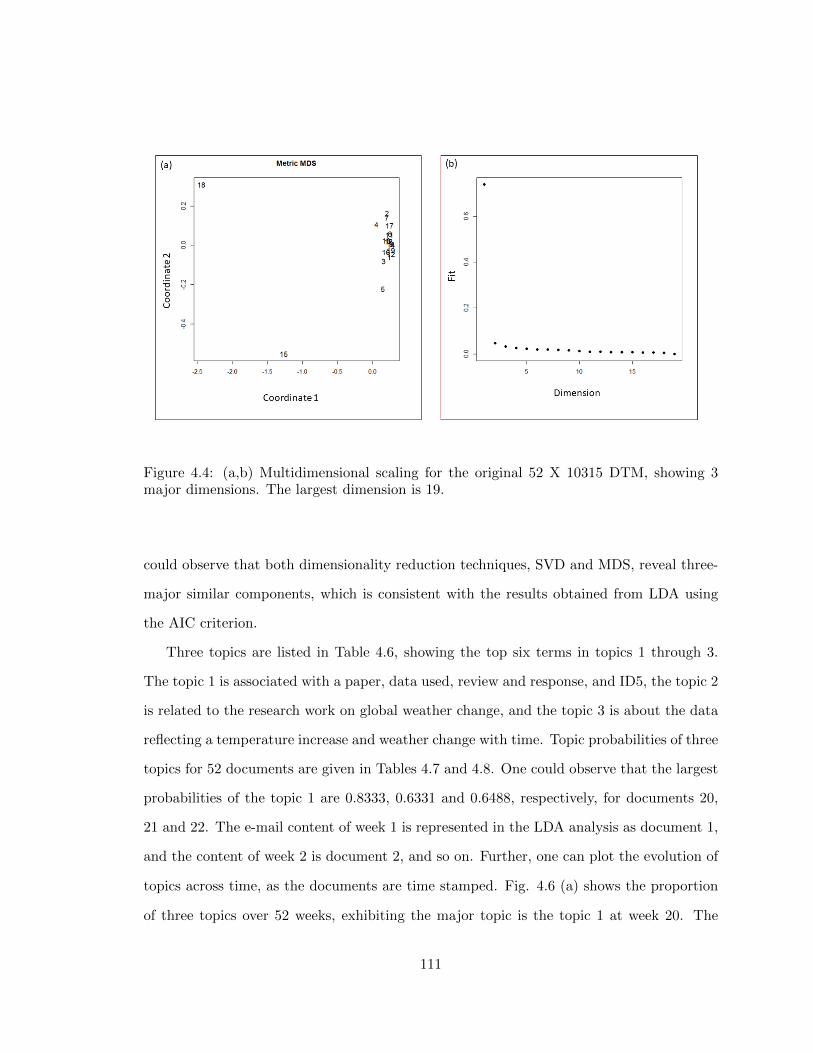
Figure 4.4: (a,b) Multidimensional scaling for the original 52 X 10315 DTM, showing 3major dimensions. The largest dimension is 19.
could observe that both dimensionality reduction techniques, SVD and MDS, reveal three-
major similar components, which is consistent with the results obtained from LDA using
the AIC criterion.
Three topics are listed in Table 4.6, showing the top six terms in topics 1 through 3.
The topic 1 is associated with a paper, data used, review and response, and ID5, the topic 2
is related to the research work on global weather change, and the topic 3 is about the data
reflecting a temperature increase and weather change with time. Topic probabilities of three
topics for 52 documents are given in Tables 4.7 and 4.8. One could observe that the largest
probabilities of the topic 1 are 0.8333, 0.6331 and 0.6488, respectively, for documents 20,
21 and 22. The e-mail content of week 1 is represented in the LDA analysis as document 1,
and the content of week 2 is document 2, and so on. Further, one can plot the evolution of
topics across time, as the documents are time stamped. Fig. 4.6 (a) shows the proportion
of three topics over 52 weeks, exhibiting the major topic is the topic 1 at week 20. The
111

Figure 4.5: (a,b) Singular value decomposition for the original 52 x 10315 DTM, showing 3dimensions.
topics are shown separately in Fig. 4.6(b).
4.8 Clustering
Two clustering methods, such as hierarchical clustering and K-means clustering, have been
applied [MC85] to the document-topic matrix to group 52 documents. For hierarchical
clustering, the agglomerative (bottom-up) hierarchical clustering method [MS02] has been
used. In this method, initially each object is assigned as a separate cluster, and a new
cluster is formed in each step by merging two clusters based on the similarity between the
clusters. Three types of similarity functions, such as single-link, complete-link, and group-
average are used in selecting clusters to merge. Here, a single - link function is used to
the document-topic matrix to cluster 52 documents. The dendrogram is given in Fig. 4.7,
showing three clusters that consist of a large cluster having 42 documents and two small
clusters with two and eight documents.
112

Table 4.2: The partial document-topic matrix.
Document Topic-1 Topic-2 Topic-3 Topic-4 Topic-5 Topic-6
1 0.0394170 0.0015138 0.0162988 0.1235568 0.0009762 0.00312672 0.0113448 0.0092984 0.0024772 0.3960651 0.0038414 0.00861633 0.0015130 0.0063491 0.0114539 0.3360106 0.0044684 0.00527444 0.0033900 0.0008414 0.0059387 0.0552899 0.0050119 0.00130485 0.0106559 0.0067150 0.0200155 0.1402126 0.0145968 0.00375936 0.0126032 0.0052728 0.0119924 0.0877407 0.0095489 0.00771627 0.0150977 0.0093834 0.0093834 0.0120501 0.0318596 0.00290728 0.2243859 0.0020768 0.0087188 0.0040303 0.0323562 0.00246759 0.1659811 0.0030672 0.0083652 0.0030672 0.0348553 0.005054010 0.0298719 0.0388809 0.0253674 0.0208629 0.0253674 0.0208629
Table 4.3: The partial T 52×19 matrix of e-mail content.
v1 v2 v3 v4 v5
1 -0.16184732 0.077103136 -0.18295134 -0.0074151010 -0.0190913892 -0.13737595 -0.270722214 -0.43221408 -0.3703561140 0.0528698963 -0.13777215 -0.061069179 -0.42583607 -0.2518886292 0.0153195424 -0.13279061 0.021356232 -0.08141087 0.0097054464 -0.0217604635 -0.13523075 0.137339256 -0.20861933 -0.0157525753 -0.0712096426 -0.14248863 0.145744288 -0.15188913 0.0355148942 -0.0699433387 -0.11550435 0.092063276 0.01841244 0.1088373227 -0.2312203708 -0.13698574 0.242338464 -0.04709021 0.0943636136 -0.0817274039 -0.14366957 0.049399435 0.03671274 0.0333295796 -0.04414884210 -0.12355908 0.148173944 -0.02858152 0.0677259471 -0.034001568
113

Figure 4.6: (a) Topic proportion of all three topics for the 52 week period around theprimary cluster using scan statistic model. (b) Topic proportion plotted separately withtime.
Table 4.4: The partial S19×19 matrix of e-mail content.
v1 v2 v3 v4 v5 v6 v7
1 3.338276 0.00000 0.00000 0.00000 0.00000 0.00000 0.000002 0.0000 0.7431123 0.00000 0.00000 0.00000 0.00000 0.000003 0.0000 0.00000 0.6079248 0.00000 0.00000 0.00000 0.000004 0.0000 0.00000 0.00000 0.5386343 0.00000 0.00000 0.000005 0.0000 0.00000 0.00000 0.00000 0.4988096 0.00000 0.000006 0.0000 0.00000 0.00000 0.00000 0.00000 0.4680062 0.000007 0.0000 0.00000 0.00000 0.00000 0.00000 0.00000 0.4589441
114

Table 4.5: The partial (D19×19)T matrix of e-mail content.
v1 v2 v3 v4 v5
1 -0.04045566 0.11565104 -0.015159817 0.047869952 -0.081602742 -0.04792393 -0.18657792 0.106860269 -0.027032479 0.014414653 -0.06423974 0.13939360 -0.012146631 0.297756953 0.788533194 -0.09435856 -0.11601124 -0.798778568 -0.493581174 0.022338195 -0.06998048 0.35691651 0.455700782 -0.739323117 0.14316247
The K-means clustering is a non-hierarchical clustering technique that divides the data
into K clusters such that the within-cluster variation is minimized[Gen02]. The objective
is to determine the optimal number of K using Calinski-Harabasz (CH) index. The null
hypothesis vs. the alternative hypothesis [CH74a], [DPL+15] is H0 : K = 1 vs. H1 : K > 1.
A pseudo-F statistic known as the CH index is defined as [CH74a], [Gen02] :
CH index =
b(k−1)w
(n−k)
, (4.15)
where b is the between cluster sum-of-square, w is within cluster sum-of-square, k is the
number of clusters and n is the number of observations. Here, k is chosen such that the
CH index is a global or a local maximum, or grows rapidly. The number of the clusters is
turned out to be 3 based on a local maximum or a rapid increase that corresponds to the
CH index of 141.58 (p-value < 0.0001). Fig. 4.8) reveals the similar structure in the reduced
dimensions, suggesting that there are three clusters with black dots indicating the centroids
of clusters. From both agglomerative and K-means clustering, three major clusters have
been obtained.
115

Table 4.6: Three major topics with top six terms obtained using the LDA from e-mailcontent around the most likely cluster.
Topic 1 Topic 2 Topic 3
data work temperaturpaper global weatheruse weather change
review new warmID-5 chang data
respons research time
Figure 4.7: Hierarchical agglomerative clustering on the document term matrix, showingthe dendrogram with three major clusters using the single link method.
116

Figure 4.8: K-means clustering showing three clusters.
4.9 Scan Statistics on Topic Proportions Using Normal Dis-
tribution
To carry out scan statistics for the time series of the maximum proportions, pt ∈ (0, 1), the
logistic transformation [Wal87] has been applied to the data. This is given by:
yt = logit pt = log
(pt
1− pt
). (4.16)
This transformation stabilizes the variance, and the transformed data become normally
distributed [BVAMF07]. Figs. 4.9(a) shows the maximum topic proportion over 52 weeks
around the most likely cluster obtained from the two-step scan process. The logistic trans-
formation of the maximum proportion is shown in Fig. 4.9(b). The normal Q-Q plot shows
that the transformed maximum topic proportion is approximately normally distributed (see
117

Fig. 4.10 ). The scan statistics have been applied here to investigate if there exists a critical
topic cluster. As discussed in chapter 1, the one-dimensional continuous scan statistic, Sw,
is the largest number of points that are observed in any subinterval of [0, T ) of length w.
Under the null hypothesis, observations x1, x2, .., xn are from the i.i.d normal distribution
with mean, µ, and variance, σ2 . For the alternative hypothesis, there would be a scanning
window of width, w, where observations are from an i.i.d normal distribution with mean, µ,
and common variance, σ2, and the observations in the rest of the intervals, [1, t) and [t+w,
n], are from an i.i.d normal distribution with mean, η, and variance, σ2 [Kul79], [Jun16].
For testing, the null hypothesis, H0 : µ = η, over the alternative hypothesis, H1 : µ > η,
the likelihood under the null hypothesis:
LH0 =n∏i=1
1√2πσ
e−(xi−µ)
2
2σ2 = (2π)−n2 σ−ne−
∑ni=1
(xi−µ)2
2σ2 . (4.17)
The log likelihood function under the null hypothesis is given by:
logLH0(µ, σ) = −n2
log(2π)− n log(σ)−n∑i=1
(xi − µ)2
2σ2. (4.18)
Taking the derivative of the log likelihood with respect to µ and setting to zero, one can
get:
∂ logLH0
∂µ= 2
n∑i=1
(xi − µ)
2σ2= 0. (4.19)
Therefore,
µ =
∑ni=1 xin
. (4.20)
118

Similarly, taking the derivative of the log likelihood with respect to σ and setting to zero,
one obtains:
∂ logLH0
∂σ= −n
σ+
n∑i=1
(xi − µ)2
σ3= 0. (4.21)
Therefore,
σ2 =
n∑i=1
(xi − µ)2
n. (4.22)
The likelihood under the alternate hypothesis:
LH1 =
(∏i∈w
1√2πσw
e−(xi−µw)2
2σ2
)(∏i 6=w
1√2πσw
e− (xi−ηw)2
2σ2w
)
= (2π)−n2 (σw)−ne
− 1
2σ2w[∑i∈w(xi−µw)2+
∑i6=w(xi−ηw)2]
.
(4.23)
The log likelihood function under the alternative hypothesis is given by:
logLH1 = −n2
log(2π)− n log(σw)− 1
2σ2w
∑i∈w
(xi − µw)2 +∑i 6=w
(xi − ηw)2
. (4.24)
By taking the derivative of the log likelihood with respect to σ and setting to zero, one
obtains:
∂ logL
∂σw= − n
σw+
1
σ3w
∑i∈w
(xi − µw)2 +∑i 6=w
(xi − ηw)2
= 0. (4.25)
Therefore, the estimated σ2w, µw and ηw are given by the following equations.
σ2w =
1
n
∑i∈w
(xi − µw)2 +∑i 6=w
(xi − ηw)2
, (4.26)
119

µw =1
nw
∑i∈w
xi, (4.27)
ηw =
∑i∈w xi
n− nw, (4.28)
where nw is the number of observations inside the window, w. The log-likelihood ratio,
log Λ, is given by:
log Λ = n log(σ) +n∑i=1
(xi − µ)2
2σ2− n
2− n log(
√σ2w). (4.29)
The maximum log-likelihood ratio is given by:
maxw
(log Λ) = maxw
(n log(σ) +
n∑i=1
(xi − µ)2
2σ2− n
2− n log(
√σ2w)
). (4.30)
Therefore, the most likely cluster can be identified when variance will be minimized.
I now apply a purely temporal scan statistic to detect the primary clusters using the
normal model to the stationary time series (See Fig. 4.11) of the transformed maximum
topic proportion, as shown in Fig. 4.9. The stationarity of the transformed series has
been confirmed by the unit root tests (see Table 4.9). The p-value is obtained using the
MC simulation with 1000 replications. A primary cluster from October 22 to November
30 2003 has been identified, which is statistically significant with the maximum LLR =
10.24 and the MC p-value = 0.01. One could see that the estimated the maximum LLR
for the primary cluster of topics is greater than the standard Monte Carlo critical value,
7.81, at the 0.0001 level of significance (See Table 4.10). In addition, it is observed that the
primary cluster consists of mostly the topic 1. It can, therefore, be concluded that the scan
statistic identifies statistically significant excessive topic activities, where mostly the topic
1 is discussed. To investigate the topic proportion, I consider here compositional approach
120

Figure 4.9: (a) The maximum proportion of topics for the 52 week period around the pri-mary cluster using scan statistic model . (b) The logistic transformed maximum proportionof topics for the 52 week period around the primary cluster using scan statistic model.
to the time series of topic 1 proportion [BVAMF07].
4.10 Time Series Models on Topic 1: Compositional ARIMA
(C-ARIMA) Model
A process of continuous proportions, pt, t = 0± 1,±2, ..., is a C-ARMA (p,q) process if for
every t [BVAMF07],
logit(pt) = φ1logit(pt−1)+ ...+φplogit(pt−p)+ logit(wt)−θ1logit(wt−1)− ....−θqlogit(wt−q),
(4.31)
where logit(wt) ∼ N(0, 2σ2w). One can write in terms of odds [BVAMF07]:
odds pt = (odds pt−1)φ1 × ...× (odds pt−p)φp × wt × (wt−1)−θ1 × ...× (wt−q)
−θq , (4.32)
121

Figure 4.10: A normal Q-Q plot of the logistic transformed maximum proportion of topicsshowing that the distribution is approximately normal.
where wt is log normally distributed. Here pt is a C-ARIMA(p, d, q) process if and only
if logit (pt) is an ARIMA (p, d, q) process. The ARIMA (p, d, q) models are well-known
statistical models for a non-stationary time series xt, and can be mathematically expressed
using backshift operator, B, as [SS06]:
φ(B)(1−B)dxt = θ(B)wt. (4.33)
Fig. 4.12 shows that the logit (topic 1 proportion) has a decreasing trend. Therefore, an
ADF regression with a trend has been applied. It is observed that the test statistic of
-3.394 is not lower than the critical value at 5% level of significance for the logit series (see
Table 4.11), suggesting that the series is not stationary. However, the first difference of the
logit(pt) series is stationary (see Table 4.12). Therefore, the logit(pt) series is an integrated
of order 1, i.e. I(1), and, as a result, the ARIMA (p, 1, q) models would be suitable.
122

Figure 4.11: Sample ACF and PACF of the logistic transformed maximum proportion oftopics series showing that the time series is stationary.
The ARIMA(0,1,1), ARIMA(1,1,0), ARIMA(2,1,0) and ARIMA(1,1,1) models have
been fitted to the logarithm of odds series. The optimal model is an ARIMA(0,1,1) based
on minimizing the AIC, and the estimated model is (see Table 4.13):
logit(pt) = −0.731logit(wt−1) + logit(wt), (4.34)
where logit(wt) ∼ N(0, 2σ2w). The standardized residual in Fig. 4.13(upper panel) at week
20, exceeds 3 times the standard deviations, indicating excessive activities. The sample
ACF of standardized residual and the Q-statistic show that the residuals are random (see
Fig. 4.13, middle and lower panels, respectively). Also, it is observed from the histogram
and the normal Q-Q plot of residuals that they are approximately normal except for an
extreme value in the right tail (see Fig. 4.14).
123
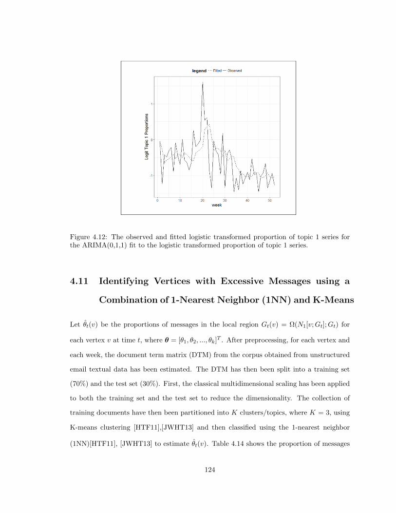
Figure 4.12: The observed and fitted logistic transformed proportion of topic 1 series forthe ARIMA(0,1,1) fit to the logistic transformed proportion of topic 1 series.
4.11 Identifying Vertices with Excessive Messages using a
Combination of 1-Nearest Neighbor (1NN) and K-Means
Let θt(v) be the proportions of messages in the local region Gt(v) = Ω(N1[v;Gt];Gt) for
each vertex v at time t, where θ = [θ1, θ2, ..., θk]T . After preprocessing, for each vertex and
each week, the document term matrix (DTM) from the corpus obtained from unstructured
email textual data has been estimated. The DTM has then been split into a training set
(70%) and the test set (30%). First, the classical multidimensional scaling has been applied
to both the training set and the test set to reduce the dimensionality. The collection of
training documents have then been partitioned into K clusters/topics, where K = 3, using
K-means clustering [HTF11],[JWHT13] and then classified using the 1-nearest neighbor
(1NN)[HTF11], [JWHT13] to estimate θt(v). Table 4.14 shows the proportion of messages
124

Figure 4.13: Time Plots of the standardized residuals, the ACF of standardized residualand the Q-statistic for the ARIMA(0,1,1) fit to the transformed topic 1.
for topic 1( θ1), topic 2( θ2), and topic 3( θ3) for week 20, 21 and 22. Here θ1 is the topic 1,
which is associated with the data used, review and ID5. This is approximately similar to
the topic 1 obtained from LDA model. It is observed that the ID1, ID5, ID7, ID10 and ID20
all have a maximum proportion of messages that are associated with the topic 1 (See Table
4.14). In order to verify this result, the betweenness associated with individuals obtained
from the metadata and the maximum topic proportions obtained from the LDA using the
textual data have been combined. Fig. 4.15 shows the time plot of the logistic transformed
maximum topic proportion, obtained from the LDA (see the bottom of Fig. 4.15) and the
time plots of betweenness of ID = 1, 5, 7, 10, 18, 20, 30 ( upper panel). One could see that
ID5, ID7, ID18, ID20, and ID30 have the maximum betweenness at week 20 and 21 (See
Fig. 4.15). The maximum betweenness represents the maximum information flow through
nodes or vertices. Therefore, it is apparent from this figure that the topic 1 (see Fig. 4.15,
125

Figure 4.14: Histogram of the residuals (top), and a normal Q-Q plot of the residuals(bottom) for the ARIMA(0,1,1) fit to the logistic transformed proportion of topic 1 series.
is mostly discussed by these individuals.
4.12 Chapter Summary
In this chapter, the scan statistic has been implemented in the unstructured text data of the
e-mail content. Such implementation of scan statistics on text data has not been done before.
Although considerable efforts have been made to extract information from unstructured
text data using text clustering, classification, and summarization, relatively few attempts
have been carried out to investigate the excessive activities associated with a particular
topic from the dynamic unstructured textual dataset. Pattern recognition and probabilistic
modeling on unstructured records, therefore, would be very useful for further research to
study fraudulent activities owing to excessive activities in communication networks. Here an
unstructured text obtained from e-mail contents around the most likely (primary) cluster,
126

Figure 4.15: Comparison between time plots of betweenness for k > 2 for different IDsobtained from metadata, and the maximum topic proportion obtained from LDA usingtextual data, showing that the excessive topic activity relating to the topic 1, which isassociated with ID = 5, 7, 18, 20 and 30 at around week 20.
from June 2003 to June 2004, has been analyzed. The major topics discussed in this period
have been identified using text mining algorithms and probabilistic modeling, such as the
latent Dirichlet allocation modeling. In the LDA modeling, the e-mail content of week 1 is
represented as document 1, and the content of week 2 is document 2, and so on. Therefore,
one can plot the evolution of topics across time, as the documents are time stamped. The
optimal number of topics has been chosen to be three, based on the minimum AIC that gives
the best fit to these data. The scan statistic based on normal distribution is then applied to
the logistic transformed maximum topic proportions to obtain the excessive topic activities.
A primary cluster from November 01 2003 until November 30 2003 has been identified,
which is statistically significant with the maximum LLR = 10.24 and the MC p-value =
0.01.
The estimated maximum LLR of the primary topic cluster is greater than the standard
127

Monte Carlo critical value, 7.81, at the 0.0001 level of significance. It can be concluded that
the scan statistic identifies statistically significant excessive topic activities, where mostly
the topic 1 is discussed. In order to identify the individuals that are discussing topic 1,
the betweenness associated with individuals from the metadata, and the maximum topic
proportions obtained from the LDA using textual data are combined. It can be concluded
that the topic 1 is mostly discussed by ID5, ID7, ID18, ID20, and ID30 at week 20 and 21.
128

Table 4.7: Topic probabilities by document obtained using the LDA method.
Topic 1 Topic 2 Topic 3
1 0.4870072 0.12114695 0.391845882 0.2248749 0.08708504 0.688040023 0.3953967 0.05042092 0.554182344 0.3805993 0.20752240 0.411878285 0.4224959 0.20279146 0.374712646 0.4445123 0.18000407 0.375483617 0.2878730 0.44406349 0.268063498 0.4775672 0.33632871 0.186104069 0.3878587 0.45540839 0.1567328910 0.3318318 0.32282282 0.3453453511 0.5010635 0.23579459 0.2631419012 0.3593337 0.23258176 0.4080845013 0.3452609 0.13375932 0.5209797714 0.2996117 0.37134682 0.3290414915 0.3434343 0.37752525 0.2790404016 0.5643217 0.13795748 0.2977208017 0.4504685 0.22958501 0.3199464518 0.4695216 0.20563272 0.3248456819 0.4957613 0.22821295 0.2760257720 0.8333829 0.07245083 0.0941662521 0.6331434 0.20236898 0.1644876522 0.6487928 0.23581982 0.1153873923 0.2960980 0.66797526 0.0359267224 0.2055872 0.66124220 0.1331706025 0.4913804 0.33741282 0.1712067426 0.4219797 0.35879763 0.2192226727 0.3964082 0.45159877 0.1519929928 0.2744511 0.49600798 0.2295409229 0.5433990 0.29066375 0.1659372730 0.2063568 0.65307906 0.14056416
129

Table 4.8: Topic probabilities by document: Continued.
Topic 1 Topic 2 Topic 3
31 0.4036814 0.29296519 0.3033533832 0.4279996 0.26344261 0.3085578333 0.3720205 0.43192312 0.1960564134 0.1886532 0.22590102 0.5854457735 0.2555714 0.48885728 0.2555713636 0.1977420 0.17560921 0.6266487837 0.2976594 0.17610977 0.5262308338 0.2239988 0.24150101 0.5345001439 0.2536991 0.23175395 0.5145469740 0.2856978 0.30749712 0.4068050741 0.2466732 0.55972087 0.1936059742 0.3687664 0.16404199 0.4671916043 0.2730443 0.57349278 0.1534628844 0.2794066 0.44432810 0.2762652745 0.1883071 0.10742160 0.7042713246 0.2648585 0.30398696 0.4311545947 0.2827147 0.37664042 0.3406449248 0.3394167 0.33512256 0.3254607349 0.2053294 0.48880170 0.3058688950 0.2409661 0.47216077 0.2868731651 0.2805110 0.34058346 0.3789055852 0.2193131 0.45579955 0.32488739
130

Table 4.9: Unit root tests on the transformed maximum topic proportion.
Unit root test Value of test statistics Lag Parameter p-value
Augmented Dickey-Fuller Test -3.7573 1 0.0284
Phillips-Perron Test -4.9454 3 0.01
KPSS Test 0.43172 1 0.0635
Table 4.10: Temporal clusters of the topic proportion showing the estimated log likelihoodratio (LLR), standard Monte critical values (SMCV) and significance level (SL) obtainedusing SaTSscan software.
Cluster Time Frame LLR p-value SMCV (SL)
Primary 11/1/03 - 11/30/03 10.240 0.01 7.81 (0.001)
Table 4.11: Unit root tests for logit (p).
Test Statistics Value of Test Statistics CV (1%) CV (5%) CV (10%)
τ3 -3.394 -4.04 -3.45 -3.15
φ2 3.9337 6.50 4.88 4.16
φ3 5.8733 8.73 6.49 5.47
131

Table 4.12: Unit root tests for the first difference logit (p) series.
Test Statistics Value of Test Statistics CV (1%) CV (5%) CV (10%)
τ3 -6.2506 -4.04 -3.45 -3.15
φ2 13.0303 6.50 4.88 4.16
φ3 19.5415 8.73 6.49 5.47
Table 4.13: ARIMA(0,1,1), ARIMA(1,1,0) and ARIMA(1,1,1) model results fitted to thelogit of topic 1 proportion series.
Parameter ARIMA(0,1,1) SE ARIMA(1,1,0) SE ARIMA(1,1,1) SE
ar1 -0.4843 0.1255 0.0912 0.1977
ma1 -0.7173 0.1106 -0.7781 0.1326
AIC 86.18 93.38 87.97
132

Table 4.14: Proportion of massages obtained from the combination of K-means and nearestneighbor.
Week ID θ = (θ1, θ2, θ3)
20 1 (0.481, 0.333, 0.037)
20 5 (0.446, 0.349, 0.059)
20 15 (0.6, 0.2, 0.000)
20 20 (0.533, 0.011, 0.367)
21 5 (0.553, 0.316, 0.079)
21 10 (0.667, 0.333, 0.000)
21 20 (0.524, 0.381, 0.048)
21 30 (0.667, 0.333, 0.000)
22 5 (0.364, 0.364, 0.136)
22 7 (0.667, 0.333, 0.000)
133

Chapter 5: Conclusions
5.1 Summary of Contributions
Around terabytes of unstructured electronic data are generated every day from twitter net-
works, scientific collaborations, organizational emails, telephone calls and websites. Fraud-
ulent activities owing to excessive communication in communication networks continue to
be a major problem in different organizations. In fact, retrieving information relating to
detection of excessive activities is computationally intensive for large data sets. Therefore,
one needs useful tools and techniques to analyze such a massive data set and detect anomaly.
In a social network, anomalies can occur as a result of abrupt changes in the interactions
among a group of individuals. Analyzing the excessive activity in a social network is thus
important to understand the fraudulent behavior of individuals in a subregion of a network.
The motivation of this research work is to investigate the excessive activities and make
inferences in dynamic sub networks. Three major contributions have been presented for to
detect anomalies of dynamic networks obtained from inter-organizational emails.
(i) Implemented Scan Statistics with variable windows, and univeriate time
series: First, a temporal scan statistic was introduced to detect clusters using the
maximum likelihood ratio as the test statistic, and betweenness as a locality statistic.
Previous studies are mostly based on the fixed and disjoint windows, and on the
assumption of short term stationarity of the series under null, which might result in
loss of information and error in detecting excessive activities. In addition, the previous
model assumed that the subgraphs are disjoint, and normalized the locality statistic
twice to eliminate the trend and assumed short-time, near-stationarity for the null
model. However, the scan statistics with fixed and disjoint scan window may not be
134

appropriate because of the occurrence of window overlaps, which may result in loss
of information on the time axis. In this research work, I implement scan statistics
with overlapping and variable window sizes to detect anomalies of dynamic networks
obtained from organizational emails. I employ the maximum likelihood ratio (LLR)
as the test statistic to rank the clusters, as the cluster size is not known. Furthermore,
I assess the structural stability and apply differencing, seasonal adjustment to make
the time series of scan statistics stationary and estimate the p-value using the Monte
Carlo (MC) simulation and the extreme value distribution, such as Gumbel, as the
exact sampling distribution of scan statistics under the null hypothesis is not known
for most of the cases. In addition, as the unstructured data set size becomes larger,
the formation of dynamic network structure is computationally intensive. Instead of
applying temporal scan statistics for ego sub networks directly, I employ scan statistics
of organizational emails with a two-step process, and use the likelihood function to
rank the clusters. I initially estimate the maximum log-likelihood ratio (LLR) to
obtain a primary cluster of communications (LLR = 82.07, p-value = 0.001) using the
Poisson model on email count series, and then extract neighborhood ego subnetworks
around the observed primary cluster to obtain more refined cluster (LLR = 644.11,
p-value = 0.001) by invoking the graph invariant betweenness as the locality statistic
using the binomial model. Furthermore, as an alternative approach, a univariate
time series has been built using the graph edit distance (GED) between subgraphs.
An autoregressive moving average (ARMA) process is then fitted to the time series,
and the anomalies were assessed using residuals obtained from the fitted model and
compared with the results obtained from the scan statistics.
(ii) Developed multivariate time series model: The second contribution is the devel-
opment of multivariate time series models, vector autoregressive (VAR) models on the
e-mail network obtained from the metadata. This represents the first known presen-
tation of the VAR model to detect excessive activities. As the scan statistics measure
the maximum of locality statistics, it can conceal the group of influential people in
135

the network. To overcome this limitation, the multivariate time series models have
been used to identify the most influential node. I fit a VAR(1) model to the multivari-
ate time series of subgraphs for each vertex using the graph edit distance to identify
anomalies. This analysis considers multiple time series simultaneously, as the nodes or
vertices of the subgraphs are interrelated. The objective of the VAR model is to iden-
tify the dynamic relationship between vertices. The excessive activities or anomalies
associated with the nodes or vertices in email network have been assessed using resid-
ual threshold. One could clearly observe the residual greater than 5 times standard
deviations at week 20 for all IDs, suggesting the occurrence of excessive activities at
this time point. From this multivariate time series analysis, it can be concluded that
the chatter has been initiated by ID = 5, and as k increases, the excessive chatter
spread among other IDs. In addition, this analysis clearly demonstrates the social
relationship between ID5 with ID1, ID7, ID10 and ID20.
(iii) Implemented scan statistics on topic models of unstructured text: The third
contribution is the implementation of the scan statistics on topic models of the un-
structured text data of e-mail content. Such implementation of scan statistics on text
data has not been done before. Although considerable efforts have been made to ex-
tract information from unstructured textual data using text clustering, classification,
and summarization, relatively few attempts have been carried out to investigate the
excessive activities associated with a particular topic from the dynamic unstructured
textual data set. Pattern recognition and probabilistic modeling on unstructured
records, therefore, would be very useful for further research to study fraudulent ac-
tivities owing to excessive activities in communication networks. Here I analyze an
unstructured textual obtained from e-mail contents around the primary cluster, June
2003 to March 2004, and investigate the major topic discussed in this period using
text mining algorithms and probabilistic modeling, such as latent Dirichlet allocation
(LDA) modeling. I then use scan statistics to get excessive topic activities. It is
observed that the topic-1, which is related to data used in a paper, has the largest
136

LLR in the neighborhood of the primary cluster using scan statistics.
(iv) One of the scientific challenges of this research includes understanding the distribution
of the organizational email subnetworks. As in one dimension, the exact distribution
of the scan statistic under the null hypothesis is only available for special cases, this
research employs other methodologies, such as Monte Carlo (MC) simulations and
the extreme value theory to estimate p-values. In addition, the size and power of the
scan statistic have been estimated. Once the sampling distribution of scan statistic is
determined, the inference on anomaly can be performed. The extreme value theory is
a statistical model that is used to model the extreme data in a given period of time,
and is based on the location-scale family. Gumbel distribution is the most well-known
distribution that belongs to this family, and has been widely used in engineering.
The present work also applies the Gumbel distribution to approximate the p-value.
Another challenge is the choice of local statistic as it provides important structural
location of a node and its neighborhood. Here I apply graph invariant, betweenness,
as a measure to identify local structure and anomaly in social networks. For building
time series of graphs, the challenges are to compute the graph distance metrics, which
are computationally intensive, and to fit time series model to assess anomalies based
on residuals.
The conclusions of this dissertation work are summarized below.
(i). The Poisson process model is employed to identify the most likely cluster of emails
using the email count data as a step-1 scan statistic process for a 10-year period.
The most likely statistically significant temporal primary cluster is detected using the
maximum LLR as the scan statistic (LLR = 82.07, p = 0.001).
(ii). The binomial model applied to network data in step-2 scan statistic process, using
betweennes as the locality statistics and the maximum LLR as the scan statistic,
detects the more refined purely temporal clusters around the primary cluster, obtained
from the step-1 scan process.
137

(iii). A univariate time series has been built using the graph edit distance metric to compare
subgraphs between two consecutive weeks. An autoregressive moving average process
is then fitted to the GED time series, and the anomalies were assessed using residuals
from the fitted model exceeding a threshold, and compared with the results obtained
from the scan statistics. The residual analysis demonstrates the statistically significant
excessive activity, consistent with the results obtained using scan statistics.
(iv). A vector autoregressive model has been fitted to the email ego-centered subnetworks.
From this multivariate time series analysis, it is concluded that the excessive chatter
has been initiated by ID5, and as k increases, the excessive chatter has been ob-
served to diffuse among ID1, ID7, ID10 and ID20. In addition, this analysis clearly
demonstrates the social relationship among ID1, ID5, ID7, ID10 and ID20.
(v). An excessive topic activity or topic chatter from the 4th week of October to 4th week
November 2003 have been identified by combining the LDA and the scan statistics.
The primary cluster consists of mostly the topic-1, which is related to data used in a
paper. Furthermore, it is concluded that ID1, ID5, ID7, ID10 and ID20 are mostly
discussing topic 1.
5.2 Future Work
This dissertation work opens up many potential areas of the future research. These method-
ologies can be applied to other networks, such as Twitter, Facebook, and telecommunication
networks. In particular, the detection of multiple excessive activities would be an area of in-
terest. These methods can be extended to investigate multiple clusters using scan statistics
with variable window sizes and overlapping windows.
The over-dispersion of the Poisson counts may occur in count data. In such cases, the
negative binomial distribution can be employed. Furthermore, one can employ the modified
ARMA models, such as integer valued ARMA (INARMA), INGARCH models to fit the
over-dispersed and correlated count data to get the critical cluster.
138

The VAR model, in chapter 4, could be extended in different ways. It would be possible
to construct a VARMA model to detect the excessive activities. If the multiple time series
is co-integrated, one could use vector error correction model (VECM) instead of the VAR
models. An interesting area for further research would be forecasting the excessive activities
using the VAR models as a part of prospective surveillance.
139

Chapter 6: Appendix A
The weekly networks (week 1 to week 4) from June 2003 to June 2004, extracted from
the e-mail edge lists, for the 52 week period are given below. Such networks have been
constructed around the most likely cluster, obtained from the two-step scan process.
140

141
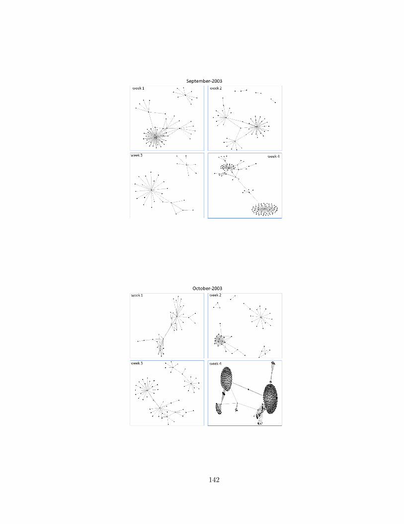
142

143

144

145

146

Chapter 7: Appendix B
Here the partial codes in R for size and power calculations and the maximum log likelihood
estimation using non-parametric method have been provided.
1. Size and Power Calculations
poisson2 <-function(M)
email <- rpois(153,158.8301)
llr = rep(0,M)
tim = rep(1,n)
SumE = 0
SumT = 0
llr = 0
for(i in 1:n)
SumE = email[i]+SumE
SumT =tim[i]+SumT
lambda1Tot = (SumE/SumT)
lambda0 = lambda1Tot
lambda1 = 158.88
A2 = log(lambda1/lambda0)
A1=(lambda0-lambda1)
llr=((SumT*A1)+(A2*SumE))
return(abs(llr))
M=1000
p2 = rep(0,M)
for(i in 1:M)
147
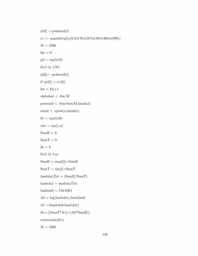
p2[i] <-poisson2(i)
cv <- quantile(p2,c(0.9,0.95,0.975,0.99,0.995,0.999))
M = 1000
Im = 0
p2 = rep(0,M)
for(i in 1:M)
p2[i]< -poisson2(i)
if (p2[i] > cv[3])
Im = Im+1
alphahat < -Im/M
poisson3 < -function(M,lamda1)
email < -rpois(n,lamda1)
llr = rep(0,M)
tim = rep(1,n)
SumE = 0
SumT = 0
llr = 0
for(i in 1:n)
SumE = email[i]+SumE
SumT = tim[i]+SumT
lambda1Tot = (SumE/SumT)
lambda1 = lambda1Tot
lambda0 = 158.8301
A2 = log(lambda1/lambda0)
A1 =(lambda0-lambda1)
llr=-((SumT*A1)+(A2*SumE))
return(abs(llr))
M = 1000
148

lambda1 = seq(from=158.81, to=170.9, by=0.1)
betahat = rep(0,length(lambda1))
powerhat = rep(0,length(lambda1))
for (j in 1:length(lambda1))
Im = 0
lamda1=lambda1[j]
p3 = rep(0,M)
for(i in 1:M)
p3[i] <-poisson3(i,lamda1)
if (p3[i] <cv)
Im = Im+1
betahat[j]<-Im/M
powerhat[j]<-1-betahat[j]
2. Maximum likelihood estimate: Non Parametric
z <- ufit(y,x = x,lmode = x[1],lc = TRUE,type = ”b”)
plot(x,y)
lines(z,col=”red”)
plot (z-h, do.points = TRUE,col.hor=”black”,col.vert=”black”,
add = FALSE,xlab=’x’,ylab=’f’)
text(1, 0.025, paste(”Mode at =”, x[1]),cex=1.0)
plot(z-x,z-y)
lines(z,type=’l’,lwd=2)
text(12,2.5e-8, paste(”Mode at =”, x[1]),cex=1.0)
qplot(zx, zy,data=df1,geom=c(”point”,”line”))
+annotate(”text”,x=10,y=2.5e-08,label=”Mode at 1”,cex=5)
z <- ufit(y,x=x,lmode=x[32],lc = TRUE,type=”b”)
149

plot(x,y)
lines(z,col=”red”)
plot(zh,do.points=TRUE,col.hor=”black”,col.vert=”black”,
add=FALSE,xlab=’x’,ylab=’f’)
text(1, 0.025, paste(”Mode at =”, x[32]),cex=1.0)
text(25,0.0e+00, paste(”Mode at =”, x[32]),cex=1.0)
qplot(zx, zy,data=df1,geom=c(”point”,”line”))
+annotate(”text”,x=25,y=2e-08,label=”Mode at 32”,cex=5)
qplot(zx, zy,data=df1,geom=c(”point”,”line”))
for (i in 1:32)
z <- ufit(y,x=x,lmode=x[i],lc=TRUE,type=”b”)
plot(x,y)
lines(z,col=”red”)
plot(zh,do.points=TRUE,col.hor=”black”,col.vert=”black”,
add=FALSE,xlab=’x’,ylab=’f’)
text(-0.05, 0.05, paste(”Mode at =”, x[i]),cex=1.0)
plot(zx, zy)
lines(z,type=’l’,lwd=2)
text(-0.05, 0.05, paste(”Mode at =”, x[i]),cex=1.0)
print(-sum(log(zy)),digits=20)
150

Bibliography
151
Bibliography
[Adl84] R. J. Adler. The supremum of a particular gaussian field. Annals of Probability,12:436–444, 1984.
[ADW94] C. Apte, F. Damerau, and S. M. Weiss. Towards language independent auto-mated learning of text categorization models. In Proc. ACM-SIGIR conferenceon Information Retrieval. Springer-Verlag New York, 1994.
[Aka73] H. Akaike. Information theory and an extension of the maximum like-lihood principle. 2nd International Symposium on Information Theory,Budapest:267–281, 1973.
[Alm83] S. E. Alm. On the distribution of the scan statistic of a poisson process.Probability and Mathematical Statistics, 5:1–10, 1983.
[Arr05] M. A. Arranz. Portmanteau test statistics in time series. Tol-Project, www.tol-project.org, 2005.
[BD93] B.E. Brodsky and B.S. Darkhovsky. Nonparametric Methods in Change-PointProblems. Springer-Science + Business Media, B.V., 1993.
[BDGH93] A. Banerjee, J. Dolado, J. Galbraith, and D. Hendry. Co-Integration, Error-correction and the Econometric Analysis of Non-Stationary Data. Oxford Uni-versity Press Oxford, 1993.
[BKNS00] M. M. Breunig, H. P. Kriegel, R. T. Ng, and J. Sander. Lof: Identifyingdensity-based local outliers. In Procedings of the 2000 ACM SIGMOD Inter-national Conference on Management of Data. SIGMOD, 2000.
[BNJ03] D. M. Blei, A. Y. Ng, and M. I. Jordan. Latent dirichlet allocation. Journalof Machine Learning Research, 3:993–1022, 2003.
[Bro08] C. Brooks. Introductory Econometrics for Finance. Cambridge UniversityPress, Cambridge, UK, 2008.
[BVAMF07] C. Barcelo-Vidal, L. Aguilar, and J. A. Martin-Fernandez. Compositionaltime series: a first approach. Procedings of the 22nd International Workshopof Statistical Modeling, Bercelona, Spain, pages 81–86, 2007.
[CD04] W. W. Chen and R. S. Deo. A generalized portmanteau goodness of fit testfor time series. Econometric Theory, 20:382–416, 2004.
152

[CG92] G. Casella and E. I. George. Explaining the gibbs sampler. American Statis-tian, 46:167–174, 1992.
[CH74a] T. Calinski and J. Harabazs. A dendrite method in cluster analysis. Commu-nications in Statistics, 3:1–27, 1974.
[CH74b] D. R. Cox and D. V. Hinkley. Theoretical statistics. Chapman and Hall,London, 1974.
[Che02] Y. T. Chen. On the robustness of ljung-box and mcleod-li q tests: A simulationstudy. Economics Bulletin, 3:1–10, 2002.
[Cle93] W. S. Cleveland. Visualizing Data. Hobart Press, Summit, New Jersey, 1993.
[CM09] P. S. P. Cowpertwait and A. V. Metcalfe. Introductory time series with R.Springer, Dordrecht, 2009.
[DBDK02] P. Dickinson, H. Bunke, A. Dadej, and M. Kraetzl. Median graphs and anoma-lous change detection in communication networks. In Information, Decisionand Control Conference. IDC-2002 Adelaide, 2002.
[DH97] A. C. Davison and D. V. Hinkley. Bootstrap Methods and Their Application.Cambridge University Press, Cambridge, United Kingdom, 1997.
[DLR77] A. P. Demster, N. M. Laird, and D. B. Rubin. Maximum likelihood fromincomplete data via the em algorithm. Journal of the Royal Statistical Society,39:1–38, 1977.
[DPL+15] R. Dalinina, V. A. Petryshyn, D. S. Lim, A. J. Braverman, and A. K. Tripati.Application of clustering techniques to study environmental characteristics ofmicrobialite-bearing aquatic systems. Biogeosciences Discussions, 12:10511–10544, 2015.
[EG87] R. F. Engle and C. W. J. Granger. Co-integration and error correction: Rep-resentation, estimation and testing. Econometrica, 55:251–276, 1987.
[Fre79] L. C. Freeman. Centrality in social networks’ conceptual clarification. SocialNetworks, 1:215–239, 1979.
[Fri03] M. Frisen. Statistical survaillance: Optimality and methods. InternationalStatistical Review, 71:403–434, 2003.
[GB99] J. Glaz and N. Balakrishnan. Scan Statistics and Applications, Statistics forIndustry and Technology. Springer Science + Business Media, LLC, New York,1999.
[Gen02] J. E. Gentle. Elements of Computational Statistics. Springer, 2002.
[Gen15] M. Genin. Discrete scan statistics and the generalized likelihood ratio test.Rev. Roumaine Math. Pures Appl., 60:83–92, 2015.
[Gla79] J. Glaz. Expected waiting time for a visual response. Biological Cybernetics,35:39–41, 1979.
153

[Gla81] J. Glaz. Clustering of events in a stochastic process. Journal of AppliedProbability, 18:268–275, 1981.
[GNW01] J. Glaz, J. Naus, and S. Wallenstein. Scan Statistics, Springer Series in Statis-tics. Springer, New York, 2001.
[GPW09] J. Glaz, V. Pozdnyakov, and S. Wallenstein. Clustering of events in a stochasticprocess, Statistics for Industry and Technology. Winsdell Publishing Company,2009.
[Gra81] C. W. J. Granger. Some properties of time series data and their use in econo-metric model specification. Journal of Econometrics, 16:121–130, 1981.
[Gra17] J. Grandell. Formulas and Survey Time Series Analysis. Avd. Matema-tisk Statistik, www.Math.kth.se/mastat/gru/sf2943/tsform, Visited Fall 2017,2017.
[GS04] T. L. Griffiths and M. Steyvers. Finding scientific topics. PNAS, 101:5228–5235, 2004.
[GW16] S. Goswami and E. J. Wegman. Comparison of classification methods forforensic research. Journal of Statistical Science and Application, 4:65–84, 2016.
[HHWB00] S. Hawkins, H. X. He, G. J. Williams, and R. A. Baxter. Outlier detectionusing replicator neural networks. In Proc. Fifth International Conference andData Warehousing and Knowledge Discovery (DaWaKO2). Aix en Provence,France, 2000.
[HN75] R. Huntington and J. Naus. A simpler expression for kth nearest neighborcoincidence probabilities. The Annals of Probabilities, 3:894–896, 1975.
[Hof99] T. Hofmann. Probabilistic latent semantic indexing. In Proceedings of the 22ndannual international ACM SIGIR conference on research and development ininformation retrieval, pages 50–57, 1999.
[Hoh08] E. L. Hohman. A Dynamic Graph Model for Representing Streaming TextDocuments,. a PhD Dissertation, 2008.
[HQ79] E. J. Hannan and B. G. Quinn. The determination of the order of an au-toregression. Journal of the Royal Statistical Society, Series B, 41:190–195,1979.
[HR05] R. A. Hannenman and M. Riddle. Introduction to social network methods.University of California, Riverside CA, 2005.
[HTF11] T. Hastie, R. Tibshirani, and J. Friedman. The Elements of Statistical LearningData Mining Inference and Prediction. Springer Series in Statistics SecondEdition, 2011.
[HXD03] Z. He, X. Xu, and S. Deng. Discovering cluster-based local outliers. PatternRecognition Letters, 24:1641–1650, 2003.
154

[Joa98] T. Joachims. Text categorization with support vector machines: learning withmany relevant features. In Proceedings of ECML-98, 10th European Conferenceon Machine Learning. Springer Verlag Heidelberg DE, 1998.
[JSTW18] D. R. Jeske, N. T. Stevens, A. G. Tartakovsky, and J. D. Wilson. Statisticalmethods for network surveillance. Applied Stochastic Models in Business andIndustry, pages 1–21, 2018.
[Jun16] I. Jung. Scan tests. In Handbook of Spatial Epidemiology, Eds. A. B. Lawson,S. Banerjee, R. P. Haining and M. D. Ugarte. Chapman and Hall, CRC Press,Taylor and Francis Group, 2016.
[JWHT13] G. James, D. Witten, T. Hastie, and R. Tibshirani. An Introduction to Sta-tistical Learning with Applications in R. Springer Series in Statistics, 2013.
[KB92] S. Karlin and V. Brendel. Chance and statistical significance in protein anddna sequence analysis. Science, 257:39–49, 1992.
[KHK09] M. Kulldorff, L. Huang, and K. Konty. A scan statistic for continuous databased on the normal probability model. International Journal of Health Geo-graphics, 8:58, 2009.
[KNT00] E. M. Knorr, R. T. Ng, and V. Tucakov. Distance-based outliers: algorithmsand applications. International Journal on Very Large Data Bases, 8:237–253,2000.
[Kre02] V. E. Krebs. Mapping networks of terrorist cells. Connections, 24:43–52, 2002.
[Kul79] M. Kulldorff. A spatial scan statistics. Communications in Statistics-Theoryand Methods, 26:1481–1496, 1979.
[LK04] H. Lutkepohl and M. Kratzig. Applied Time Series Econometrics. CambridgeUniversity Press Cambrigde, 2004.
[LK05] A. Lazarevic and V. Kumar. Feature bagging for outlier detection. In Proc.
11th ACM SIGKDD international conference on Knowledge Discovery in DataMining, pages 157–166, 2005.
[LM81] W. Li and A. McLeod. Distribution of the residual autocorrelations in mul-tivariate arma time series models. J. Roy. Statist. Soc. Ser. B, 43:231–239,1981.
[Lov68] J. B. Lovins. Development of a stemming algorithm. Mechanical TranslationComputational Linguistics, 11:22–31, 1968.
[Lut06] H. Lutkepohl. New Introduction to Multiple Time Series Analysis. Springer-Verlag New York, 2006.
[Mar12] D. J. Marchette. Scan statistics on graphs. WIREs. Comput. Stat., 4:466–473,2012.
155

[MBB17] S. Moritz and T. Bartz-Beislstein. inputets: Time series missing value inpu-tation in r. The R Journal, 9:207–218, 2017.
[MC85] G. W. Miligan and M. C. Cooper. An examination of procedures for deter-mining the number of clusters in a data set. Psychometrika, 50:159–179, 1985.
[MGW92] B. Masand, L. Gordon, and D. Waltz. Classifying news stories using memorybased reasoning. In Proceedings of the 15th annual international ACM SIGIRconference on Research and development in information retrieval. ACM PressNew York, 1992.
[MM16] W. L. Martinez and A. R. Martinez. Computational Statistics Handbook withMATLAB. CRC Press, 2016.
[MS02] C. D. Manning and H. Schutze. Foundations of Statistical Natural LanguageProcessing. The MIT Press, Cambridge, Massachusetts, 2002.
[Nau65] J. Naus. The distribution of the size of the maximum cluster of points on aline. Journal of the American Statistical Association, 60:532–538, 1965.
[Nau82] J. Naus. Approximation for distribution of scan statistics. Journal of theAmerican Statistical Association, 77:377–385, 1982.
[NCS02] B. V. North, D. Curtis, and P. C. Sham. A note on the calculation of empericalp values from monte carlo procedures. American JOurnal of Human Genetics,71:439–441, 2002.
[New63] G. F. Newell. Distribution for the smallest distance between any pair of kth
nearest-neighbor random points on a line. In Time Series Analysis, Proceed-ings of the Conference. Brown University (Ed., M. Rosen-blatt), New York:Academic Press, 1963.
[New10] M. E. J. Newman. Networks: An Introduction. Oxford University Press,Oxford OX2 6DP, 2010.
[NP95] S. Ng and P. Perron. Unit root tests in arma models with data dependentmethods for the selection of the truncation lag. Journal of the AmericanStatistical Association, 90:268–281, 1995.
[NP01] S. Ng and P. Perron. Lag length selection and the construction of unit roottests with good size and power. Econometrica, 69:1519–1554, 2001.
[PCMP05] C. E. Priebe, M. J. Conroy, D. J. Marchette, and Y. Park. Scan statistics onenron graphs. Computational Mathematical Organization Theory, 11:229–247,2005.
[Pfa06] B. Pfaff. Analysis of Integrated and Cointegrated Time Series with R. Springer-Verlag New York, 2006.
[Pfa08] B. Pfaff. Var, svar and svec models: Implementation within r package vars.Journal of Statistical Software, 27:1–32, 2008.
156

[PGKS05] V. Pozdnyakov, J. Glaz, M. Kulldorff, and J. M. Stllele. A mertingale approachto scan statistics. Ann. Inst, Statist. Math., 57:21–37, 2005.
[Pin05] B. Pincombe. Anomaly detection in time series of graphs using arma processes.ASOR Bulletin, 24:2–10, 2005.
[POH98] C. E. Priebe, T. Olson, and D. M. Healy. A spatial scan statistic for stochasticscan partitions. Journal of the American Statistical Association, 92:1476–1484,1998.
[PPM+10] C. E. Priebe, Y. Park, D. J. Marchette, J. M. Conroy, J. Grothendieck, andA. L. Gorin. Statistical inference on attributed random graphs: Fusion ofgraph features and content: An experiment on time series of enron graphs.Computational Statistics and Data Analysis, 54:1766–1776, 2010.
[PS00] M. D. Porter and R. Smith. Network neighborhood analysis. In Intelligenceand Security Informatics (ISI). IEEE International Conference, 2000.
[Ren94] E. Rennison. Galaxy of news: An approach to visualizing and understandingexpansive news landscapes. In ACM Symposium on User Interface Softwareand Technology, 1994.
[Rob67] T. Robertson. On estimating a density which is measurable with respect to aσ-lattice. The Annals of Mathematical Statistics, 38:303–358, 1967.
[Rub87] D. B. Rubin. Multiple imputation for nonresponse in surveys. John Wiley andSons, 1987.
[Sch78] G. Schwarz. Estimating the dimension of a model. Annals of Statistics, 6:461–464, 1978.
[Sch89] G. W. Schwert. Tests for unit roots: A monte carlo investigation. Journal ofBusiness and Economic Statistics, 7:147–160, 1989.
[SG07] M. Steyvers and T. L. Griffiths. Probabilistic topic models. Handbook of latentsemantic analysis, 427:424–440, 2007.
[Sim80] C. A. Sims. Macroeconomics and reality. Connections, 48:1–48, 1980.
[SKM10] R. S. Sparks, T. Keighley, and D. Muscatello. Early warning cusum plansfor surveillance of negative binomial daily disease counts. Journal of AppliedStatistics, 37:1911–1929, 2010.
[SKR99] P. J. Shoobridge, M. Kraetzl, and D. Ray. Detection of abnormal change in dy-namic networks. In Information, Decision and Control Conference (IDC’99).IDC’99 Adelaide, 1999.
[SM83] G. Salton and M. J. McGill. Introduction to Modern Information Retrieval.McGraw-Hill Inc. New York, 1983.
[Sol08] J. L. Solka. Text data mining: theory and methods. Statistics Surveys, 2:94–112, 2008.
157

[SPST+01] B. Schlkopf, J. C. Platt, J. Shawe-Taylor, A. J. Smola, and R. C. Williamson.Estimating the support of a high-dimensional distribution. Neural Computa-tion, 13:1443–1471, 2001.
[SS06] R. H. Shumway and D. S. Stoffer. Time series analysis and its applicationswith R examples. Springer Texts in Statistics) 2nd Edition, 2006.
[SSBM96] G. Salton, A. Singhal, C. Buckley, and M. Mitra. Automatic text decomposi-tion using text segments and text themes. In Proceedings of the seventh ACMconference on Hypertext. ACM Press New York, 1996.
[Sta10] T. Stadnitska. Deterministic or stochastic trend: Decision on the basis of theaugmented dickey-fuller test. Methodology, 6:83–92, 2010.
[Str99] D. W. Stroock. Probability theory: an analytic view. Cambridge UniversityPress, 1999.
[Sut12] C. D. Sutton. Nonparametric Statistics: Order Statistics, Quantiles and Cov-erages. Class notes (Stat 657), George Mason University, 2012.
[SWY75] G. Salton, A. Wong, and L. S. Yang. Spatial scan statistics adjusted formultiple clusters. Journal of the American Society for Information Science,18:613–620, 1975.
[SZ10] X. Shao and X. Zhang. Testing for change points in time series. J. Am. Stat.Association, 105:1288–1240, 2010.
[SZY+14] D. Savage, X. Zhang, X. Yu, P. Chou, and Q. Wang. Anomaly detection inonline social networks. Social Networks, 39:62–70, 2014.
[Tsa14] R. S. Tsay. Multivariate time series analysis with R and financial applications.Wiley, 2014.
[VA80] P. Vacek and T. Ashikaga. An examination of the nearest neighbor rule fotimputing missing values. Proc. Statist. Computing Sect, pages 326–331, 1980.
[Wal87] K. F. Wallis. Time series analysis of bounded economic variables. JournalTime Series Analysis, 8:115–123, 1987.
[Weg70] E. J. Wegman. Maximum likelihood estimation of a unimodal density function.The Annals of Mathematical Statistics, 41:341–364, 1970.
[Weg90] E. J. Wegman. Hyperdimensional data analysis using parallel coordinates.Journal of American Statistical Association, 85:664–675, 1990.
[Weg11] E. J. Wegman. Order restricted inference: computational algorithms. JointStatistical Meetings, Miami, Fl, 2011.
[Wei07] C.H. Weiss. Controlling correlated processes of poisson counts. Quality andreliability engineering international, 23:389–400, 2007.
[Wei09] C.H. Weiss. Modelling time series counts with overdispersion. Statistical Meth-ods and Applications, 18:507–519, 2009.
158

[WN74] S. Wallenstein and J. Naus. Probabilities for the size of the largest clusters andsmallest intervals. Journal of the American Statistical Association, 69:690–697,1974.
[WN87] S. Wallenstein and N. Neff. An approximation for the distribution of the scanstatistic. Statistics in Medicine, 12:1–15, 1987.
[WT09] C.H. Weiss and M. C. Testik. Cusum monitoring of first-order inter-valued au-toregressive processes of poisson counts. Journal of quality technology, 41:349–400, 2009.
[ZAK10] Z. Zhang, R. Assuncao, and M. Kulldorff. Spatial scan statistics adjusted formultiple clusters. Journal of Probability and Statistics, 64:2379–2389, 2010.
[ZCP+15] W. Zhao, J. J. Chen, R. Perkins, Z. Liu, W. Ge, Y. Ding, and W. Zou. Aheuristic approach to determine appropriate number of topics in topic model-ing. BMC Bioinformatics (suppl 13), 16:S8, 2015.
[ZW06] E. Zivot and J. Wang. Modeling financial time series with S-PLUS. Springer,New York, NY, 2006.
159

Curriculum Vitae
Suchismita Goswami earned B.Sc (Horns) in Mathematics from Krishnath College, Cal-cutta University and M.Sc. in Applied Mathematics from Vidyasagar University, India.She worked as a lecturer in Berhampore college, India, where she taught linear algebra andcalculus after her graduation. She then moved to Stony Brook, NY and enrolled in theMS program in Applied Mathematics and Statistics (Operation Research) at SUNY StonyBrook in 2000, and graduated in 2001. She completed an MS in Epidemiology and Bio-statistics in 2009, and MS in Statistical Science in 2013 from George Mason University. Sheenrolled in the PhD program in Computational Science and Informatics (CSI) at GeorgeMason University in Fall 2013. She worked at the World Health Organization, Washington,DC as a summer intern on the development database and statistical modeling of Malaria.She has presented her work in national and international conferences. She chaired sessionson Time Series Models and Bioinformatics at an SDSS conference in 2018. She published ajournal paper, entitled Comparison of Different Classification Methods on Glass Identifica-tion for Forensic Research Journal of Statistical Science and Application, April 2016, Vol.4, No. 03-04, 65-84 doi: 10.17265/2328-224X/2015.0304.001, and another journal paper(under progress), Detection of Excessive Activities in Time Series of Graphs, Journal ofApplied Statistics, communicated February 2019.
160