detecting ransomware in encrypted network traffic using
TRANSCRIPT

Detecting Ransomware in Encrypted Network Traffic Using
Machine Learning
by
Jaimin Modi
B.Eng., Gujarat Technological University, 2014
A Thesis Submitted in Partial Fulfillment
of the Requirements for the Degree of
Master of Applied Science
in the Department of Electrical and Computer Engineering
© Jaimin Modi, 2019
University of Victoria
All rights reserved. This thesis may not be reproduced in whole or in part, by photocopy or other
means, without the permission of the author.

ii
SUPERVISORY COMMITTEE
Detecting Ransomware in Encrypted Network Traffic Using
Machine Learning
by
Jaimin Modi
B.Eng., Gujarat Technological University, 2014
Supervisory Committee
Dr. Issa Traore, Department of Electrical and Computer Engineering Supervisor
Dr. Kin Li, Department of Electrical and Computer Engineering
Departmental Member

iii
ABSTRACT
Ransomware is a type of malware that has gained immense popularity in recent time due to its money
extortion techniques. It locks out the user from the system files until the ransom amount is paid.
Existing approaches for ransomware detection predominantly focus on system level monitoring, for
instance, by tracking the file system characteristics. To date, only a small amount of research has focused
on detecting ransomware at the network level, and none of the published proposals have addressed the
challenges raised by the fact that an increasing number of ransomware are using encrypted channels for
communication with the command and control (C&C) server, mainly, over the HTTPS protocol.
Despite the limited amount of ransomware-specific data available in network traffic, network-level
detection represents a valuable extension of system-level detection as this would provide early indication
of ransomware activities and allow disrupting such activities before serious damage can take place.
To address the aforementioned gap, we propose, in the current thesis, a new approach for detecting
ransomware in encrypted network traffic that leverages network connection and certificate information
and machine learning. We observe that network traffic characteristics can be divided into 3 categories –
connection based, encryption based, and certificate based. Based on these characteristics, we explore a
feature model that separates effectively ransomware traffic from normal traffic. We study three different
classifiers – Random Forest, SVM and Logistic Regression. Experimental evaluation on diversified dataset
yields a detection rate of 99.9% and a false positive rate of 0% for random forest, the best performing of
the three classifiers.
iv
Contents
List of Tables ................................................................................................................................................ vi
List of Figures .............................................................................................................................................. vii
ACKNOWLEDGEMENTS ................................................................................................................................... viii
DEDICATION ................................................................................................................................................... ix
Chapter 1 Introduction .............................................................................................................................. 1
1.1 Context .......................................................................................................................................... 1
1.2 Research Problem ......................................................................................................................... 3
1.3 Approach Outline .......................................................................................................................... 5
1.4 Thesis Contribution ....................................................................................................................... 6
1.5 Thesis Outline ................................................................................................................................ 7
Chapter 2 Background and Related Works ................................................................................................ 8
2.1 Background ................................................................................................................................... 8
Ransomware Anatomy .......................................................................................................... 8
Execution Characteristics .................................................................................................... 12
2.2 Related works ............................................................................................................................. 15
2.2.1 Static analysis ...................................................................................................................... 15
2.2.2 Network-based Dynamic Analysis ....................................................................................... 17
2.2.3 System-based Dynamic Analysis ......................................................................................... 18
2.2.4 Other Approaches ............................................................................................................... 20
2.2.5 Malware Detection in Encrypted Network Traffic Approaches .......................................... 22
2.3 Summary ..................................................................................................................................... 24
Chapter 3 Datasets .................................................................................................................................. 25
3.1 Ransomware Dataset .................................................................................................................. 25
3.1.1 Experiment set up ............................................................................................................... 26
3.2 Normal Dataset ........................................................................................................................... 29
3.3 Network Activity Data from Bro IDS Log Files ............................................................................. 30
3.3.1 Generating log files ............................................................................................................. 30
3.3.2 Interconnection of log files ................................................................................................. 32
3.4 Labelling the data ........................................................................................................................ 33
3.5 Final Dataset ............................................................................................................................... 33
3.6 Summary ..................................................................................................................................... 34

v
Chapter 4 Features Model ....................................................................................................................... 35
4.1 Creating flows ............................................................................................................................. 35
4.2 Feature Definitions ..................................................................................................................... 40
4.2.1 Conn.log features ................................................................................................................ 40
4.2.2 Ssl.log features .................................................................................................................... 43
4.2.3 X509.log features ................................................................................................................ 44
4.3 Summary ..................................................................................................................................... 48
Chapter 5 Experiments and Results ......................................................................................................... 49
5.1 Dataset Information .................................................................................................................... 49
5.2 Data Preparation/Preprocessing ................................................................................................. 50
Handling missing data ......................................................................................................... 51
Splitting the data ................................................................................................................. 51
Data Transformation ........................................................................................................... 52
Data Imbalance ................................................................................................................... 52
Hyperparameter Tuning ...................................................................................................... 53
5.3 Performance Metrics .................................................................................................................. 54
5.4 Results ......................................................................................................................................... 55
Logistics Regression ............................................................................................................ 56
Random Forest .................................................................................................................... 61
SVM ..................................................................................................................................... 63
5.5 Summary ..................................................................................................................................... 66
Chapter 6 Conclusion ............................................................................................................................... 67
6.1 Summary ..................................................................................................................................... 67
6.2 Future Work ................................................................................................................................ 68
Chapter 7 References .............................................................................................................................. 70

vi
List of Tables
Table 3. 1 – Count of ransomware samples in each family for ISOT dataset ............................................. 26
Table 3. 2 – Total number of records from log files in the dataset ............................................................ 34
Table 5.1 – Count of flows for individual family ......................................................................................... 50
Table 5.2 – Accuracy score for the classifiers for ‘train_test_split’ set (with and without SMOTE)........... 55
Table 5.3 – Accuracy score for the classifiers for 10-fold cross validation set (with and without SMOTE) 56
Table 5.4 – Detection rate (DR) and False Positive Rate (FPR) for the classifiers over test dataset .......... 56
Table 5.5 – Classification report for logistic regression classifier ............................................................... 57
Table 5.6 – Classification report for random forest classifier ..................................................................... 62
Table 5.7 – Classification report for SVM classifier ..................................................................................... 64

vii
List of Figures
Figure 2. 1 – Phishing email from the TeslaCrypt ransomware campaign ................................................... 9
Figure 2. 2 – Ransomware lifecycle ............................................................................................................... 9
Figure 2. 3 – A sample ransom note from TeslaCrypt ransomware ........................................................... 12
Figure 2. 4 – General ransomware network communication flow ............................................................. 13
Figure 3. 1 – Ransomware dataset collection environment setup ............................................................. 27
Figure 3. 2 – Cuckoo sandbox directory structure for report files [37] ...................................................... 28
Figure 3. 3 – Generating log files from Bro IDS ........................................................................................... 30
Figure 3. 4 – Interconnection of log files .................................................................................................... 33
Figure 4.1 – Bro log files connection information....................................................................................... 36
Figure 4.2 – Connecting log files to create dataset .................................................................................... 39
Figure 4.3 – Computing periodicity in a flow .............................................................................................. 42
Figure 4.4 – Determining validity of a certificate from the time of capture .............................................. 45
Figure 4.5 – Determining certificate age for a packet ................................................................................ 46
Figure 5. 1 – Comparing confusion matrix for logistic regression classifier (with and without SMOTE) .... 57
Figure 5. 2 – ROC curve for logistic regression classifier ............................................................................ 58
Figure 5. 3 – Confusion matrix for logistic regression classifier after applying hyperparameter tuning ... 60
Figure 5. 4 – Comparing confusion matrix for random forest classifier (with and without SMOTE) ......... 61
Figure 5. 5 – ROC curve for logistic regression classifier ............................................................................ 62
Figure 5. 6 – Comparing confusion matrix for SVM classifier (with and without SMOTE) ......................... 63
Figure 5. 7 – ROC curve for SVM classifier .................................................................................................. 64
Figure 5. 8 – Confusion matrix for support vector machine classifier after applying hyperparameter
tuning .......................................................................................................................................................... 65

viii
ACKNOWLEDGEMENTS
I would like to express my sincere gratitude to my supervisor Dr. Issa Traore for providing me this
opportunity to pursue my studies and research at the University of Victoria. I am greatly indebted to Dr.
Issa Traore for providing me access to the ISOT laboratory and research facilities. Without his precious
encouragement, guidance and financial support, it would not have been possible to conduct this research.
Also, I would like to thank Dr. Kin Fun Li, Dr. Neil Ernst for being on my thesis committee.
I am lucky to meet good friends and colleagues through this journey, beginning from when I
arrived in Victoria to guiding me in research during difficult phases. I would to thank my first employer
Infosys Ltd. for introducing me to the IT world in best possible way. I would also like to acknowledge
University of Victoria for providing a beautiful campus with all best events, sporting facilities, TA & co-op
opportunities. I am grateful to HighTechU and team for extending my skills on a new path. Finally, I am
always indebted to pillars of my strength, my loving parents and sister for trusting in me to travel my own
journey.

ix
DEDICATION
To my Pillars of Strength,
Mom, Dad, Ishani and my nieces Hiva & Aanshi

1
Chapter 1 Introduction
1.1 Context
With the growing number of Internet users, the scope of malware attacks is also increasing. Malware is
created by malicious authors with an intent to invade, damage or disable electronic devices. Within the
broad categories of malware, ransomware has gained threatening popularity in the modern Internet
world.
Ransomware is a piece of software written with the purpose of disabling access to data in return for
money. It locks out the users from their personal devices until the demanded ransom is paid by the user.
It relies on strong encryption techniques that make it impossible for anyone to decrypt the files without
using the private key. Since its inception, ransomware has evolved and leveraged sophisticated techniques
to make it harder to crack. The first ransomware attack, named AIDS Trojan, occurred in 1989 and was
distributed using floppy disk [1]. Instead of executing immediately, it waited for users to boot their system
90 times. It encrypted all the system files after that and demanded users to pay $198. The code had many
flaws, which enabled experts to decrypt the infected files.
With the advancement of ransomware, the majority of the ransomware attacks have occurred in recent
years. The cybercrime magazine, Cybersecurity Ventures, predicted that ransomware damages could
reach $20 billion by 2021 [2]. The healthcare and financial service industries are among the hardest hit.
The WannaCry ransomware attack costed England’s National Health Service (NHS) more than $100 million
in damage recovery [3]. CryptoLocker ransomware alone managed to infect more than 500 thousand
computers worldwide, gaining close to $3 million dollars in ransom fees [4]. GandCrab ransomware, first
detected in January 2018, has already collected about $300 million in ransom.

2
Ransomware can be categorized into different types based on its implementation. However, 2 major types
of ransomware that have had the most impact include locker ransomware and crypto ransomware. Locker
ransomware locks the system and prevents users from using it. Crypto ransomware encrypts the files in
the machine making it inaccessible to the user. Rather than encrypting the whole hard disk, it searches
for specific file extensions only.
The ultimate motive for any ransomware author is to maximize their financial gain while making their
identity untraceable. Cryptocurrency such as Bitcoin enables the authors to collect the money while hiding
in plain sight.
Maintaining adequate communication channel between an infected device and the command and control
server (C&C) is an essential characteristic of modern malware. Increasingly, such communications are
taking place using web protocols. Hypertext Transfer Protocol (HTTP) over SSL, also called HTTPS is a
protocol for secure communications over the Internet. The advantage of using HTTPS protocol is that the
communications are encrypted and only the designated user can decrypt the data. According to Lets
Encrypt, an open and free Certificate Authority (CA), 79% of the web pages loaded by Firefox users were
using HTTPS protocol [5]. As per Google transparency report of July 2019, 94% of Google products are
encrypted. The report also states that more than 85% of pages loaded by desktop users are using HTTPS
protocol. With the increase in encrypted network traffic, the malware authors have also started shifting
towards utilizing HTTPS for secure communication. A 2016 Cisco report observed that while the majority
of the malicious traffic used unencrypted HTTP, there is a steady 10-12% increase in malicious
communication over HTTPS. One year later, Cyren, a leading enterprise cybersecurity service provider
reported that 37% of malware now utilize HTTPS. It also stated that every major ransomware family since
2016 has used HTTPS communication [6].

3
1.2 Research Problem
There are currently different approaches for ransomware detection, including static analysis, dynamic
analysis and reverse engineering.
Static analysis approach involves detecting malware using signatures based on rules. These rules are
designed based on the previously known ransomware behaviors. Signature-based detection involves a
repository of rules that generate alerts if any malicious routine in the binary code matches a rule. The
repository needs to be updated continuously over time as new ransomware are released. This approach
is not helpful to detect novel ransomware. Cyber criminals use sophisticated techniques such as code
obfuscation to evade static-based detection systems easily.
The limitations of signature-based detection approaches put emphasis on designing improved techniques
for detecting ransomware. Reverse engineering involves decomposing the malware binary and studying
the raw assembly form of the malware for better insights. This helps researchers in establishing a better
understanding of the program execution and analyze the patterns within it. However, with the increasing
complexity of ransomware, the process of disassembling it is becoming complicated. This also makes it
difficult to identify matching patterns if the code is obfuscated. Since reverse engineering for large number
of families is time consuming and resource intensive, the focus is now shifting towards dynamic analysis.
Dynamic analysis can be divided into system level and network level approaches. Most of the work done
till now on network-level dynamic ransomware detection system has focused on studying a specific or a
relatively small number of families [7] [8]. Also, most of the approaches using machine learning only
involves basic features that can easily be evaded by ransomware authors by making necessary
modifications [9].

4
Even though a significant amount of work has been done on system level for detecting ransomware using
dynamic analysis, not enough work has been conducted on network level. Network level dynamic analysis
approach involves live monitoring of network traffic data to identify anomalous behaviour. This includes
analyzing all the network communications over TCP/HTTP protocol such as duration, payload bytes, etc.
The fact that, to date, only a handful of works have been conducted on detecting ransomware at the
network level could be due to the limited amount of ransomware-specific information available in
network traffic data compared to system level data. On one hand, because of the scarcity of such
ransomware-specific data in network traffic, identifying and processing such information poses significant
challenges. On the other hand, the development of an efficient and effective network level detector can
represent a valuable extension of system level detection as this would provide early indication of
ransomware activities and allow disrupting such activities before serious damage can take place.
Network level detection is made more complicated because, as aforementioned, malware
communications are increasingly carried over HTTPS encrypted channels. Proper analysis of such traffic
also involves studying (besides standard packet features) the certificates exchanged and all the key
insights within it. HTTPS communication is encrypted and hence it is almost impossible to decrypt the
payload. Only a limited amount of research have been published on detecting malware in encrypted traffic
[10] [11] [12] [13]. All these works have focused on general malware; to our knowledge, no previous work
has addressed the challenges pertaining to ransomware specifically. Even though Cabaj et al. [7] worked
on detecting ransomware that used encrypted network traffic, the research does not put emphasis on
HTTPS traffic detection. Similarly, although research work conducted in [8] [14] [9] include ransomware
samples that communicate using HTTPS protocol, the proposed approaches do not address the detection
of malicious encrypted network traffic.

5
A key characteristic of ransomware is the connection with the C&C server for downloading malicious
scripts and key exchange. Since, increasingly, the communication happens over secure channel,
anomalous traffic packets hide amongst the normal traffic packets. Moreover, the newer variants of
ransomware exchange the payload in small amounts to avoid detection. Another aspect of secured
network traffic is certificate exchange. Certificates are based on digital signatures issued by Certificate
Authorities (CA) with a specific validity period providing authenticity of the webpage. Modern
ransomware families use digitally signed certificates that are within the validity period. This deceives the
browser in trusting the web servers (hosting the ransomware C&C) while these may be executing
malicious scripts at the backend. Hence digitally signed webpages can no longer be considered safe. Due
to such multiple factors involved, there is a need to develop a new network level ransomware detection
approach that will address the aforementioned challenges.
The purpose of the current thesis is to address this gap by developing a machine learning model that
involves a diversified feature set that combines the unique characteristic of ransomware and encrypted
network connections. We explore a feature model that is based on the properties of connections,
encryption characteristics and certificate information. We study 3 different machine learning classifiers
to identify the model with best detection rate and least false positive rate.
1.3 Approach Outline
The main idea behind our approach is that ransomware exhibits different behavioural characteristics from
normal data flow. Our proposed approach involves studying network data that involves different
ransomware families. The study allows identifying features that differentiate ransomware packets from
normal packets. We use an inspiration from a previous work on general malware detection from
encrypted traffic by Strasak [13] to develop our initial feature model.

6
The approach consists of generating initially log files from network captures using BRO Intrusion Detection
System (IDS). We construct flows by aggregating network packets from the log files and calculate the
feature values. The features are based on three dominant characteristics – connection based, encryption
based, and certificate based. We utilize a wide variety of ransomware families and normal traffic data for
constructing diversified dataset to evaluate our approach.
Three machine learning classifiers – Random Forest, SVM and Logistic Regression – are explored.
Experimental evaluation results are presented for balanced and imbalanced dataset. Additionally, we
tuned hyperparameters for each classifier to achieve the best results.
For the current work, we utilize Brothon library for creating the flow and building our dataset. Any network
traffic data has normal traffic in majority amount and ransomware traffic in low amount. Since this case
occurs for any network traffic, the data will always be imbalanced. Hence, we used data resampling
techniques to achieve better results. Our experimental evaluation shows that ransomware traffic, despite
being in small portion, can be identified within the majority amount of normal traffic data. We are also
able to achieve a low false positive rate, which underscores the importance of data sampling.
1.4 Thesis Contribution
The main contribution of the thesis is a new model for detecting ransomware from encrypted network
traffic. As aforementioned, while there are few published works on either network level ransomware
detection models or generic network level malware detection models, to our knowledge, the current
thesis makes the first proposal on encrypted network level detection focused specifically on ransomware.
The proposed model consists of a unified set of features that enables detecting ransomware from the
network traffic data. This is an important step towards detecting emerging ransomware, those that evade

7
current network-based detection system. Experimental evaluation on collected ransomware and normal
dataset, yields for random forest, the best performing of 3 the classifiers, a detection rate (DR) of 99.9%
and a false positive rate (FPR) of 0%, which are relatively good, considering the wide of variety
ransomware families involved in the evaluation dataset.
1.5 Thesis Outline
The outline of this thesis is as follows. Chapter 1 gives an outline of the context of the research, by
highlighting the different terminologies, the types of ransomware and ransomware economics, and by
stating the research problem.
Chapter 2 provides background information on ransomware, its technical execution characteristics and
then summarize and discuss related works. Chapter 3 presents the ISOT dataset collection procedure and
describes its different components. Chapter 4 introduces the proposed features and describes their
extraction methodology. Chapter 5 presents the dataset cleaning process, the training of the machine
learning models, and the experimental evaluations. Chapter 6 makes concluding remarks and discusses
future work.

8
Chapter 2 Background and Related Works
In this chapter, we give an overview of ransomware by studying its general lifecycle. We also analyze its
execution characteristics within network traffic. Furthermore, we review previous research work
conducted in relation to ransomware. We categorize the related works based on the approaches used by
the researchers and place a particular emphasis on network traffic analysis-based approaches which are
more closely related to the current thesis.
2.1 Background
Ransomware Anatomy
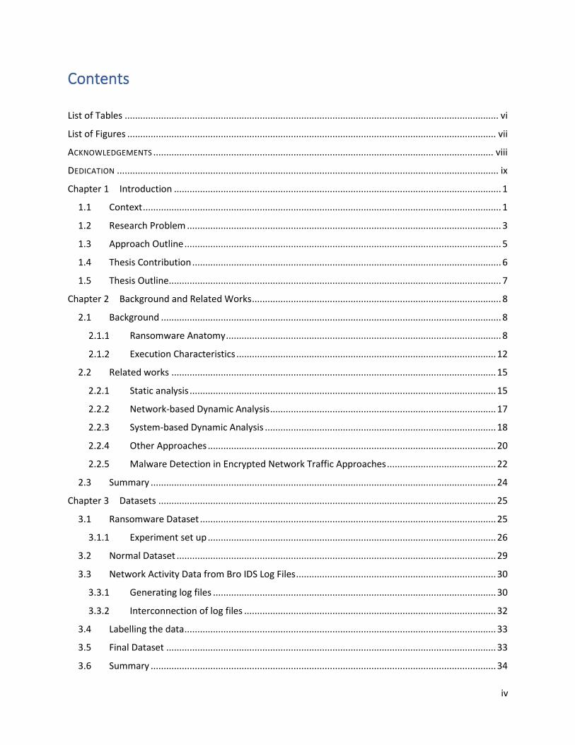
Generally, ransomware spreads through various social engineering tactics, such as phishing emails
containing malicious attachments, spam emails that redirect users to unsafe websites, etc. Ransomware
authors lure victims in taking actions by falsely claiming, for instance, that their machines are virus
infected or they need to follow some security advisory to keep their accounts and devices safe. Another
popular method for spreading ransomware is using exploit kits (EKs) [15]. Exploit kits are automated
software packages that search for vulnerabilities within browser-based applications. This usually starts by
the user landing on a compromised webpage. Figure 2.1 illustrates one such phishing email that forces
the user to download the attachment.
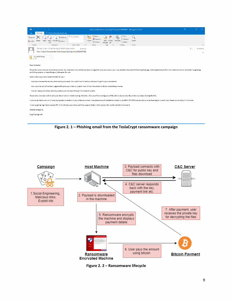
The main motive of ransomware is to encrypt user’s files. The general ransomware lifecycle is illustrated
in figure 2.2.
9
Figure 2. 1 – Phishing email from the TeslaCrypt ransomware campaign
Figure 2. 2 – Ransomware lifecycle

10
Once the malicious payload is downloaded by the user on the machine, it will start executing in the
backend. Ransomware hides its identity by using a host file known as dropper file for its execution.
Ransomware authors consider the possibility of system reboot. Hence, the executable payload is installed
in the reboot registry key and system start-up process as well so that it remains persistent across reboot.
Once the executable file runs on the machine, the ransomware will contact the command and control
(C&C) server by sending all the host machine information. Once the information is received by the C&C
server, it will respond back with the encryption keys that are needed to encrypt the files. Ransomware
starts the encryption process once it receives the keys from the server. The ransomware will first encrypt
the data on local drive followed by data files on removable media and then targeting files on local network
(mapped drives, network shares). Since ransomware encrypts large volume of files, it may take hours or
days to complete the encryption process.
The modern ransomware families use hybrid encryption approach by utilizing both symmetric and
asymmetric encryption [16]. In symmetric encryption process, the same key is used for encryption and
decryption. The sender and receiver share a common key. Some common symmetric algorithms used by
ransomware authors are the Advanced Encryption Standard (AES), Rivest Cipher 4 (RC4), etc. The
advantage of using symmetric encryption is its speed due to low computational requirement. The
disadvantage is using the common key which puts emphasis on keeping the key secure. Asymmetric
encryption, also known as public key encryption, uses 2 keys – one for encryption and one for decrypting
it. This pair of keys are also known as public and private keys. The public key can be distributed through
the web to the world outside, while only the user possesses the private key. This way only the private key
can decrypt the messages encrypted with the corresponding public key. Some common asymmetric
cryptography algorithms used by ransomware authors are Diffie-Hellman-Merkle, Rivest-Shamir-Adleman
(RSA) and Elliptic Curve. Asymmetric cryptography has the advantage of authenticity because only the

11
intended user can decrypt the data. However, it consumes a lot of computational resources while costing
significant amount of time. In the hybrid approach, the ransomware payload receives a symmetric key
(e.g. using AES) along with an asymmetric public key (e.g. using RSA) from the C&C server. Since the
asymmetric encryption would be time consuming, it first encrypts all the files using the symmetric AES
key. The large volume files are encrypted easily and then the AES keys are encrypted using the asymmetric
RSA public key. This way the files can only be decrypted using the RSA private key which is owned by the
ransomware author.
All the communications between the C&C server and the infected machine are secured by the TOR
browser. The ransomware creates a thread to download the TOR browser for anonymous communication.
Important services such as Windows error reporting tools, Windows antivirus and Windows updates are
disabled. It also deletes the Windows backup copy to make the system unrecoverable. Once it encrypts
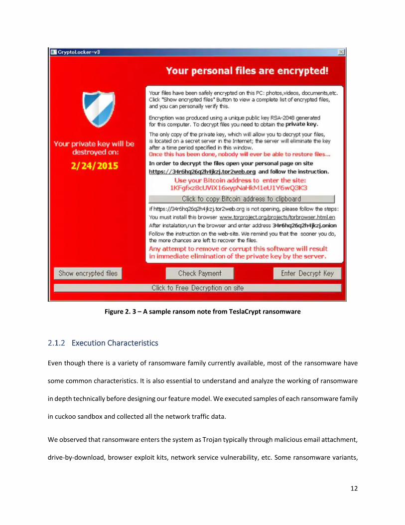
all the desired files, it will display a ransom note as shown in figure 2.3. The ransom note informs the
victim that the machine has been hacked and all the files are encrypted along with all the payment
information. The authors generally create a new unique virtual currency account for each user to make
the payment untraceable.
Virtual currency such as Bitcoin has become the de facto currency for payment. Unlike conventional
currency, bitcoin transactions are completely anonymous which makes it difficult to trace the creator of
the ransomware. Bitcoin payment is fast, reliable and verifiable. Furthermore, they can even automate
the process of releasing the private key upon receiving the payment. Some authors also prefer payment
using prepaid cards or some other methods like PaySafeCard or Ukash [17].
12
Figure 2. 3 – A sample ransom note from TeslaCrypt ransomware
Execution Characteristics
Even though there is a variety of ransomware family currently available, most of the ransomware have
some common characteristics. It is also essential to understand and analyze the working of ransomware
in depth technically before designing our feature model. We executed samples of each ransomware family
in cuckoo sandbox and collected all the network traffic data.
We observed that ransomware enters the system as Trojan typically through malicious email attachment,
drive-by-download, browser exploit kits, network service vulnerability, etc. Some ransomware variants,

13
such as Locky, exploit the vulnerabilities embedded in Microsoft Word document to enter the victim’s
machine. Once the payload is in the machine, the characteristics can be divided into two broad types
based on payload execution – host-based and traffic-based characteristics.
We study the traffic-based characteristics since we design our feature model based on the network data.
The communication between the C&C server and infected machines happens in 4 general stages [7]. These
stages are depicted in figure 2.4.
Figure 2. 4 – General ransomware network communication flow
Depending on the family, ransomware uses different technique to communicate with the C&C server.
Some ransomware families, such as Cerber, use hardcoded URL to communicate with the proxy, while
some use direct IP addresses. With its evolution, modern ransomware utilizes a Domain Generation

14
Algorithm (DGA) to communicate with the proxy server. DGA produces thousands of potential domain
names on the go in order to disguise the detection system. The communication is often SSL-encrypted.
The C&C servers are remotely located to avoid exposing them and are often privately owned by the
authors. Sometimes the proxy servers are located on infrastructure operated by legitimate third parties
such as Cloudflare.
During the first stage, the payload communicates with the C&C server with its unique identifier. This
unique identifier helps the malware author manage the list of all infected machines by generating its
personal code. The payload also shares information related to the host machine such as IP address, MAC
address and OS version. While on the host side, the payload searches for different file extensions and
starts encrypting the files using the symmetric encryption algorithms (e.g. based on AES 128-bits or 256-
bits).
During the second stage, the C&C server’s response contains the personal code for the victim’s machine,
an image containing all the ransomware information, TOR address link for the payment information and
RSA public key. The communication is HTTP POST-based making it secure by encryption. The malicious
payload then downloads all the required malicious scripts from the proxy. After this stage, the
symmetrically encrypted files are encrypted asymmetrically using the RSA public key. This asymmetric
encryption mostly uses the RSA-2048 or RSA-4096 bits algorithms. The reason for applying asymmetric
encryption over the symmetric encryption is to make decryption almost impossible. The private key to
decrypt the files is kept secure by the ransomware author.
During the third stage, the ransomware payload on the victim’s machine sends back the
acknowledgement for the public key reception.
The final stage occurs once all the files are encrypted. During this stage, the ransomware reports the end
of the encryption process with the number of files encrypted.

15
The above steps correspond to the general response cycle followed by ransomware families. Some
ransomware variants such as CryptoWall 4.0 skip the last step of reporting the completion process. While
Locky ransomware exchanges the public key during the third stage [7]. However, all the steps are covered,
in general, during these four phases of communication.
During the encryption process, the encrypted files overwrite the original files making the file recovery
difficult. The ransomware also detects and removes any OS shadow copy in the system to make the data
unrecoverable. The ransomware goes through each directory searching for specific file formats embedded
in the malicious script. Generally, file formats from productivity suites such as Microsoft Office, media
files, and so on, are targeted. While going through each directory, it also generates help files containing
all the payment related information.
2.2 Related works
Ransomware detection has been studied extensively in recent years. Several works have been conducted
related to ransomware for its detection and counteraction. These existing works can be divided into three
major categories – static, dynamic and general. Depending on what level ransomware execution activities
are detected, existing models can also be classified into network-level, host-level and hybrid [7]. We
review a sample of these works in the following.
2.2.1 Static analysis
Schultz and Zodin [18] conducted one of the earliest research works in detecting malware using data
mining methods. The authors used Portable Executables (PE), string information and byte sequences to
classify malware using Naïve Bayes classifier. The experiment was conducted using 3,265 malware binaries

16
and 1,001 benign programs. The classifier yielded a detection rate of 97.96% and a false positive rate of
3.8%.
Kolter et al. [19] proposed a similar malware detection system based on n-gram byte sequence. The
classifiers used during the experiment were Naïve Bayes, Decision Trees, SVM and boosted decision tree.
Boosted decision tree achieved the best result with a True Positive Rate (TPR) of 98% and a False Positive
Rate of 5%.
Han and colleagues [20] proposed a malware analysis method by using visualized images and entropy
graphs. The method involved converting the block of opcode into RGB color image.
Jerome et al. [21] translated malware binaries into sequence of opcodes using the program opcodes of
malware. The authors observed some new signature patterns that helped improve the false positive rate
(FPR) and false negative rate (FNR) of the classifier. The dataset consisted of 15,670 instances of benign
applications and 11,960 instances of malign applications. The authors utilized information gain (IG) for
feature selection and SVM for machine learning classification. The model achieved a detection rate of
96.83% and a recall value of 81.4% for malware detection.
The static detection method relies on hard coded rules based on past malware attacks. Hence, static
detection methods cannot detect any new malware variants. Moreover, these detection methods can be
evaded using code obfuscation techniques. While conducting a study on ransomware detection using
static analysis, Kharaz observed that only 10 engines out of 60 could detect ransomware [4]. Moser et al.
[22] conducted experiments to test the limits of advanced static detection systems to detect malware.
They rewrote three well-known worms that static-based antivirus systems were not able to detect. Baig
et al. [23] evaded static detection by modifying packed portable executables.

17
2.2.2 Network-based Dynamic Analysis
In 2018, Cabaj and colleagues [7] studied two crypto ransomware families – CryptoWall and Locky. The
study explored the network communication characteristics for both ransomware families. They observed
that the interactions of ransomware are based on HTTP POST messages in 3 major stages – registration
with C&C server, exchanging public keys for encryption, and acknowledging successful encryption. They
proposed a Software Defined Networking (SDN)-based detection approach where a vector containing the
payload values from the aforementioned 3 stages is built and the corresponding centroid is calculated.
After optimizing a threshold value, new samples can be predicted based on the value of the centroid. The
experimental evaluation was based on 250 samples of CryptoWall and Locky each, and around 13,000
normal samples. The evaluation yielded a detection rate of 97-98% with 4-5% of false positives. The
detection system is designed such that it measures the threshold value of payload. Such system can be
evaded by ransomware authors by dividing the ransomware payload amount such that it appears as
normal payload to the detection system. Also, the experiment is based only on 2 ransomware families.
Omar et al. [9] introduced NetConverse, a model to detect Windows ransomware using machine learning
classification. The model aggregates packets into unique conversations based on 5-tuple – protocol,
source/destination IP address, source/destination port values. They extracted 9 feature values, and used
a dataset consisting of 210 ransomware samples and 264 goodware samples collected from VirusTotal.
Various machine learning classifiers were studied including Bayes Network, Multilayer perceptron, J48,
KNN, Random forest, and LMT. The accuracy of 97.1% was obtained using J48 classifier (their best
performing classifier) with a false positive rate of 1.60%. Despite the relatively high accuracy, the feature
model consists of very basic features, such as the total number of bytes, duration, and IP addresses.
Modern ransomware can easily evade such feature model.

18
Almashhadani et al. [8] presented a comprehensive behavioural analysis by using Locky ransomware for
case study. The authors used a dataset containing 6 locky ransomware samples and 10 normal samples
collected from various trustable sources. They extracted 18 features that were further classified into
packet-level and flow-level features. Random forest, LibSVM, Bayes Net and Random tree machine
learning classifiers were used for prediction. Random tree achieved the best accuracy of 97.92% for
packet-based feature model with a false positive rate of 0.021%. For flow-based feature model, Bayes net
obtained the highest accuracy of 97.08% with 0.029% false positive rate. However, the model was based
only on a single ransomware family, which is not very representative of the current state of the
ransomware landscape in which many other families are prevalent.
Wan et al. [14] propose a flow-based system Biflow by aggregating the packet-based data. The exact size
of the dataset was not provided, but samples from only 2 ransomware families – Locky and Cerber – were
used for the experiment. After selecting 36 features, the data was trained on J48 decision tree machine
learning classifier. A maximum precision of 90.19% was achieved when 19 features were selected and
selecting 36 features gave 89.12% precision. The experiment, however, does not provide enough proof
on the results obtained in terms of detection rate and false positive rate. Also, the experiments are based
on just 2 ransomware families.
2.2.3 System-based Dynamic Analysis
In this section, we review some research work carried out on system-level.
Kharaz et al. [4] analyzed ransomware attacks that occurred between 2006 and 2014. The authors
explored file system activity and types of I/O request packets to the file system for detecting ransomware.
The study was carried on 15 different ransomware families with the conclusion that almost 94% of
samples implement simple locking or encryption techniques. They also studied the bitcoin payment
method used by the ransomware authors. It was observed that transactions happened in short period of

19
activity, with small bitcoins amount. However, even after suggesting multiple counteraction strategies, no
experimental evaluation was conducted by the authors.
In yet another follow up work, Kharaz and colleagues [24] proposed a ransomware detection system called
UNVEIL. The model was based on system-level activities such as memory usage, processor usage, and disk
I/O rate for behavioural detection. The model also uses text analysis to analyse the threatening notes and
checks for screen lockers by capturing screenshots at regular intervals. The experiment yielded an
accuracy of 96.3% for ransomware detection. Despite of achieving relatively high accuracy, the model
lacks early detection capability for ransomware. It also fails to provide a backup mechanism. Also, the
proposed system is passive and ineffective for newer ransomware samples.
Continella et al. [25] proposed a ransomware-aware self healing system called ShieldFS, a competitor to
UNVEIL. The system also extended its capability by providing roll back feature. It computes the entropy of
the write operations combined with the frequency of read, write and folder listing operations. The system
also scans the memory for any processes that it considers potentially malicious while searching for block
cipher key schedules. However, the newer ransomware deletes all the shadow copy in the file system,
making the recovery almost impossible. Additionally, the memory scanning aspect is time consuming and
hence the chances of finding the key in the memory is rare.
Daniele et al. [26] developed EldeRan, a machine learning approach for analyzing and detecting
ransomware. The model works in two phases. After monitoring a set of activities, Elderan extracts a set
of features in the first phase. In the second phase, the features such as API calls, dropped files, registry
keys, and directory files are trained using machine learning model. The authors tested EldeRAN using SVM
and Naïve Bayes machine learning classifiers on 582 ransomware samples from 11 different families. The
model yielded an accuracy of 96.3% after applying some feature selection techniques. However, the
model mostly uses only binary features for detection, such as absence or presence of registry key

20
operations, DLL operations, etc. In new ransomware variants, some operations may be completely absent,
and the proposed binary features will fail to detect it. This makes the model ineffective in those cases.
Chen et al. [27] also presented a machine learning based ransomware detection model. The model was
based on creating call flow graph by monitoring API call sequences of ransomware binaries and
transforming them into a set of features. The model used Random Forest, SVM, Naïve Bayes and Logistic
Regression machine learning classifiers on 168 ransomware samples. Logistic Regression achieved the
highest accuracy of 98.2% with a false positive rate of 1.2%. The model only focuses on limited set of
features to detect ransomware, which could be easily evaded by newer ransomware.
Scaife et al. [28] developed an early-detection system called CryptoLock based on three primary indicators
for file changes – file type changes, similarity measurement and Shannon entropy. A scorekeeping
mechanism aggregates the scores from each of the three indicators and based on the threshold value, it
triggers a detection indicator. The experiment was conducted on 492 ransomware samples belonging to
14 different families obtained from VirusTotal. The model achieved 100% detection rate with zero false
positive and less than 10 files lost per sample before encryption. Despite achieving perfect detection rate,
the system is unable to distinguish whether a user or a ransomware is encrypting the data. This can
generate false positives even if the user is just compressing the file.
2.2.4 Other Ransomware Detection Approaches
Salehi and colleagues [29] worked on detecting ransomware using Domain Generated Algorithms (DGA).
They extracted 3 classes of features for the detection engine – random and gibberish characters in
domain, frequency of different domains, and replication of same domains. The detection engine also
includes a black/white domain list to decrease the number of false positives. The model achieved a
detection rate of 100% on 20 ransomware samples. The false positive rate and false negative rate both

21
were zero. However, the model was featured such that it detects only DGA based samples and cannot
detect any non-DGA ransomware.
Hasan and Rahman [30] presented a machine learning based framework called ‘RansHunt’ to detect
ransomware that integrates both static and dynamic analysis. The static features included Function Length
(FLF) and Printable String Information (PSIT). The dynamic features were the same as used in the EldeRan
system. The dataset consisted of 360 ransomware binaries and 923 benign samples and the model was
trained using SVM classifier. It yielded a detection rate of 97.1% and an FPR of 3%. Since the static features
were not effective and the dynamic features produce the same result as previous works, the model will
be ineffective in detecting new ransomware.
Recently, several works have been published on ransomware detection for mobile phones and the
Internet of Things (IOT). Andrionio et al. [31] proposed an Android ransomware detection system called
HelDroid. It is a static analysis system based on threatening text recognition that utilizes the ransom note
to detect coercion. It also relies on two other indicators of compromise – encryption detector that checks
if read, write, delete functions are called within memory and locking detector that is based on designed
heuristic. However, detection based on ransom note is not much useful as the mobile phone will be locked
by then.
Karimi and Moattar [32] presented an optimal approach of transforming sequence of executable binaries
into grey scale image. They also worked on improving the performance of the model by using dimension
reduction technique based on Linear Discrimant Analysis (LDA) for separating two or more classes. The
model was tested using two different datasets. The first experiment was conducted using 140
ransomware samples and 20 benign samples yielding an accuracy of 97%. The second experiment was
conducted using 230 ransomware samples and 30 benign samples yielding an accuracy of 97.3%.

22
Azmoodeh and Ali [33] proposed a detection approach of ransomware in IoT networks based on the
energy consumption of the android devices. The machine learning classifier used were k-Nearest Neighbor
(KNN), Neural Network (NN), Support Vector Machine (SVM) and Random Forest (RF). The dataset
consisted of 1260 ransomware samples and 227 normal samples. KNN yielded the highest accuracy of
94.27% with detection rate of 95.65%.
2.2.5 Approaches for Malware Detection in Encrypted Network Traffic
Prasse et al. [10] utilized neural network to detect malware in encrypted network traffic. The dataset was
collected from different small to large computer networks that use Cisco AnyConnect Secure Mobility
Solution. The dataset was divided as current data or future data for further analysis. While the current
dataset contained 350,220 malicious flows and 43,150,605 benign flows, the future dataset consisted of
955,037 malicious flows and 142,592,850 benign flows. The experiment consisted of analysing 3 different
domain name-based feature set – engineered features, character n-gram features and neural domain-
name features. The model utilized LSTM neural network and random forest classifiers for detection.
Experiment results showed that neural network achieves the best result at a 73% recall rate and a
precision of 90% for neural domain-name features. Experimental evaluation also concluded that the
model can detect malware approximately 90 minutes after its first occurrence in the system.
Anderson el al. [11] proposed a machine learning based approach to identify malware in encrypted
malware traffic. The model consisted of 20 features from 3 different domains – TLS data, DNS data and
HTTP data. The logistic Regression and SVM machine learning classifiers were used for prediction. The
dataset was collected manually using a sandbox environment that generated 13,542 malicious flows and
42,927 benign flows. The experimental results showed that logistic regression achieved the best results
with an accuracy of 99.978% and a false detection rate of 0.00%.

23
In yet another work by Anderson at Cisco [12], the proposed approach included 7 different features that
utilized the random forest machine learning classifier. The dataset consisted of 2,638,559 benign flows
and 57,822 malicious flows. The experimental evaluation consisted of varying the threshold value of the
random forest classifier, with 0.5 being the default threshold for classification. The model also focused on
representing the accuracy results for malware and benign samples separately. The model achieved best
accuracies of 99.99% and 85.80% for benign and malware, respectively, at 0.95 threshold value.
Strasak [13] also proposed a machine learning based approach for detecting malware in encrypted
network traffic. The approach utilized bro for generating different log files and utilizing them to extract
features. The model consisted of 28 features based on 3 different domains – encryption-based,
connection-based and certificate-based. While some dataset was collected from various sources [34]
[35], the normal dataset was captured manually by browsing through the common websites. The
complete dataset consisted of 60,977,061 malicious connection records and 770,401 normal connection
records. Flows were constructed from the records using the 4-tuple (source IP, destination IP,
destination port and protocol) methodology. The following machine learning classifiers were utilized:
SVM, neural network, random forest and XGBoost. Experimental evaluation show that XGBoost
achieved the best results with a detection rate of 94.96% and a false positive rate of 1.89%. Even though
the proposed model achieves a high detection rate, the ratio of malicious data to normal data is very
high. Also, the evaluation dataset does not include ransomware data. This puts emphasis on our current
work, where we utilize ransomware data for detection. Our model also works on achieving a better false
positive rate compared with the previous approach.

24
2.3 Summary
In this chapter, we started by discussing general ransomware lifecycle and its network communication
characteristics. We then summarized and discussed related work on ransomware detection.
Ransomware classification using static analysis is not enough for detecting new variants. Furthermore,
dynamic detection system is more effective than static based system for the detection of novel
ransomware. From the above literature analysis, we can also note that even though more emphasis is put
on file system activity, not enough work has been done on network based dynamic analysis. The existing
works are either on very specific families or basic feature set.
With evolving ransomware, the network communication activities will also change to avoid detection.
Strong feature set is required to detect all such future ransomware.

25
Chapter 3 Datasets
Data collection is an essential step for building a strong machine learning model. The prediction of the
model is as effective as the data from which it is built. To our knowledge, there is no publicly available
ransomware detection dataset. It has been decided at the ISOT lab to fill this gap by collecting a new
dataset to be shared with the research community. The collected dataset includes both network files and
file activities generated from ransomware as well as benign applications.
The data required for the current research are network activity files. These files are captured in form of
packets known as pcap files and can be analyzed using Wireshark application. For our research work, we
collect 2 kinds of network traffic data – ransomware and normal. We describe in this chapter the
corresponding dataset.
3.1 Ransomware Dataset
All the ransomware binaries were collected from well-known antivirus aggregator VirusTotal [36].
VirusTotal scans for all binaries through all its 70 antivirus scanners. Therefore, it is trustworthy to
download the binaries from VirusTotal website. The binaries are executable files that can be launched in
safe environment for further analysis. The binaries collected in the ISOT dataset consist of 666 different
samples from 20 different ransomware families. These families are the most prevalent versions of
ransomware currently available. Table 3.1 provides a detailed breakdown of ransomware samples from
each family.
Family Number
of Samples
CTBLocker 2
Cerber 122

26
CryptoShield 4
Crysis 8
Flawed 1
GlobeImposter 4
Jaff 3
Locky 129
Mole 4
Petya 2
Sage 5
Satan 2
Spora 5
Striked 1
TeslaCrypt 348
Unlock26 3
WannaCry 1
Win32.Blocker 18
Xorist 2
Zeta 2
Total 666
Table 3. 1 – Count of ransomware samples in each family for ISOT dataset
3.1.1 Experiment set up
Once the ransomware is executed, we can understand its behaviour, the changes it incurs and the
underlying motive. While ransomware binaries are deployed, we can capture all data related to network
traffic. All binaries were executed following established and commonly agreed principles inside an open
source automated malware system – the cuckoo sandbox [37]. The environment setup is described in
figure 3.1.
Cuckoo sandbox is made up of two components – cuckoo host and guest analysis machine. Cuckoo host
runs on the host machine (Ubuntu in our case). It is responsible for starting the analysis for a susceptible
file and generating reports using cuckoo result server. The guest analysis machine is where the analyst

27
can install multiple virtual machines and run the binaries. We use VirtualBox as the guest analysis machine
and Windows 7 as the virtual Operating System (OS).
The Windows 7 OS is loaded with all necessary software, such as Python, Java, Microsoft Office, etc. It
also has controlled access to the Internet via NAT adapter. Outbound traffic to any other machine in the
local environment was blocked so that other machines in the network are not affected. The Windows
firewall was disabled, and no other processes were running while executing the ransomware.
Figure 3. 1 – Ransomware dataset collection environment setup
With the help of python command line tool available in cuckoo host, we execute the ransomware binaries
in the guest analysis machine. After running a couple of binaries for full execution time, we concluded
that 30 minutes threshold was enough for capturing important elements. All the ransomware binaries
were then executed for 30 minutes while capturing the execution traces of the ransomware. The

28
Operating System (OS) was rolled back to a clean state after each execution. This way, we get the original
traces for all ransomware samples.
The cuckoo result server runs simultaneously with the ransomware execution and collects all the changes
done inside the guest machine in form of report files. Multiple report files are collected for each binary.
The output data are stored in a specific directory format. Figure 3.2 shows the directory structure for
storing all the output files.
Figure 3. 2 – Cuckoo sandbox directory structure for report files [38]
The different types of report files generated are described as below [38]:
- analysis.log
This log is generated by the analyzer while execution happens inside the guest machine. It reports creation
of processes, files and any errors occurred during the execution.
- dump.pcap

29
This file contains all the data related to network traffic. It is generated by a network sniffer, such as
tcpdump. We use this file for all our further analysis.
- memory.dmp
This file contains the memory dump of the guest analysis machine.
- files/
This directory contains all the files that cuckoo was able to dump and were used by malware for changes.
- logs/
This directory contains all the logs generated by cuckoo process monitoring.
- reports/
Based on the configurations edited in cuckoo’s configuration file, this directory will contain all the reports.
- shots/
While malware is executing on the guest analysis machine, all the screenshots are captured and stored in
this directory.
3.2 Normal Dataset
The normal (i.e. benign) dataset was collected in 2 different ways - manual data collection and network
files from the Stratosphere project [39].
The manual data collection was done while keeping Wireshark on capture mode and visiting Alexa top
100 websites. The duration for each capture was 30 minutes and 30 total samples were collected. Each
sample was collected by manually browsing through the websites on Alexa top 100 list.

30
The Stratosphere Intrusion Prevention System (IPS) project has a sister project called Malware Capture
Facility Project [39] that is responsible for capturing all kinds of data. The data is organized in a specific
directory structure for easy access. We wrote a python script to download 10 pcap files from the
Stratosphere dataset web portal [40].
3.3 Network Activity Data from Bro IDS Log Files
Bro Intrusion Detection System (IDS) is an open-source framework that, besides its intrusion detection
capability, is most commonly used as network traffic analyzer [41]. Its powerful set of features cover areas,
such as deployment, analysis, scripting language and interfacing. Amongst its many features, the one that
we utilise in the current research is the comprehensive set of log files that record network activities. These
log files can be utilised for offline intrusion analysis and forensics. Log files can be easily visualized and
manipulated using dataframe structure.
3.3.1 Generating log files
After collecting the data in pcap format, we utilize Bro IDS for converting network activity data into log
files. These log files contain essential information for feature extraction. Figure 3.3 explains the process
in detail.
Figure 3. 3 – Generating log files from Bro IDS

31
Bro IDS has a core engine which is called event engine. The event engine is responsible for streaming
filtered packets into high-level distilled information. This information reflects the underlying network
activity on various levels such as connection level, application level and activity level. Policy script
interpreter plays a major when there are manual scripts written while data is streamed through it. The
final output consists of multiple log files [42], including the following:
- conn.log – UDP/ICMP/TCP connections
- dns.log – DNS traffic activity
- files.log – Files analysis result
- ssl.log – SSL/TLS handshake info
- http.log – HTTP requests and reply
- x509.log – Certificates related information
We use only 3 types of log files for our feature extraction in the current thesis. These log files contain
adequate information about the encrypted traffic. More details on these log files are provided below.
1. Conn.log – Connection record
Each line in the conn.log contains information about packets that flow between two IP addresses. It
contains multiple columns such as IP address, protocols, ports, number of packets, duration, label, etc.
2. Ssl.log – SSL record
This log file contains all information related to the SSL/TLS handshake that helps encrypt all the data
between 2 endpoints. It has also the information about which certificates were used during the encryption
process. It includes important columns such as SSL/TLS version number, server name, cipher suite used
and many more.

32
3. X509.log – Certificates record
Certificates are issued by certificate authorities that ensure the credibility of the web server. This log file
contains all information related to the certificate records involved during SSL handshake. The columns
describe information, such as validity time, certificate serial number, signature algorithms used and many
more.
3.3.2 Interconnection of log files
The advantage of using the log files is that they are interconnected with each other through unique
identifiers (id). This helps in extracting complete information for any given packet for further inspection.
The log files are easy to load as dataframe and hence the connection can easily be analysed. Figure 3.4
explains the interconnection of log files in detail.
The ‘uid’ column connects the conn.log and ssl.log files. As observed from the figure 3.4, uid |
Cq2MdB2HCZqC9MHmDj| connects these 2 log files. The ‘cert_chain_fuids’ column in the ssl.log connects
all the corresponding certificate records in the x509.log file.
The certificates are issued by certificate authorities (CA) of two types – root CA and intermediate CA. A
browser considers a CA to be trusted if it is included in the browser trusted CA list. Not all intermediate
CAs are present in the browser trusted list. For an intermediate CA to be trusted, it should have been
issued by another trusted intermediate CA or the root CA. When a user visits a website, the browser
checks if the CA is included in the browser trusted CA list. If not, then it will check the certificate of the
issuing CA. This way it continues in the certificate chain until it finds a CA that is present in the trusted list.
This chain is present in the ssl.log file as the ‘cert_chain_fuids’ column. Each unique value in this column
has a corresponding certificate record details in the x509.log file.

33
3.4 Labelling the data
There are 3 kinds of label that we use in the current thesis – normal, ransomware and background. After
checking each source IP address on VirusTotal, we label it as normal or ransomware. If no information is
available, it is labeled as background. The background labeled data is not used in the current thesis. All
the labelling is done in the conn.log file.
conn.log
ts uid src ip src port dst ip dst port protocol
1387314871.7356 Cq2MdB2HCZqC9MHmDj 10.0.0.46 37965 173.194.112.24 443 tcp ssl
1387314878.6469 CN1K411P0lvgtKjko7 10.0.0.46 40417 173.194.112.14 443 tcp
1387314569.6284 CULb0W3zRUNSNc7fsg 10.0.0.46 45563 85.17.73.216 54081 tcp
ssl.log
ts uid … cert_chain_fuids
1387314871.7636 Cq2MdB2HCZqC9MHmDj …
1387314878.6775 CN1K411P0lvgtKjko7 … Fmp6nt24djwkItG0j9, FvPTai39Gf9eKP0p4i, FWaIP33OHTt1odn4ah
1387315821.5367 CZR65Y3qNu4pNMzPqd … Fbs6W94vtdjUe6Dmsc, FpIKMO3eRmlyYbNYXh
x509.log
ts uid version serial
1387314878.7129 Fmp6nt24djwkItG0j9 3 6511A5752828358E
1387314567.6265 Fbs6W94vtdjUe6Dmsc 3 39571D1CACE1944DDEBAC4A9D7273B27
1387314569.6284 FvPTai39Gf9eKP0p4i 3 1E22C737A3915E3FAB65C4B5A41CAE46
Figure 3. 4 – Interconnection of log files
3.5 Final Dataset
We collected a total of 45 normal samples and 666 ransomware samples. These samples, when processed
through the Bro IDS give out log files. Table 3.2 shows the final numbers of records involved in the

34
combined dataset in terms of each log file. This dataset is then used for feature extraction in upcoming
chapter.
Log file Count
Normal Ransomware Total
Connection records (conn.log) 1,010,157 883,582 1,893,739
SSL records (ssl.log) 79,832 10,890 90,722
Certificate records (x509.log) 63,159 13,604 76,763
Total 1,153,148 908,076 2,061,224
Table 3. 2 – Total number of records from log files in the dataset
3.6 Summary
In this chapter, we discuss the dataset collection process. The ransomware dataset was collected in a safe
environment set-up using cuckoo sandbox. The required binaries were obtained from VirusTotal. The
normal dataset was collected from various trusted sources. Some normal dataset was also collected by
manually browsing the web pages. Bro IDS was utilized for generating various log files.

35
Chapter 4 Features Model
In this chapter, we present our feature model, and explain in detail the creation of a flow dataset from
the Bro log files. The flow dataset provides the basis to extract the features that will be classified using
machine learning.
4.1 Creating flows
After collecting the log files through Bro IDS, the next step is to preprocess the data and calculate the
feature values. Before calculating the feature values, it is important to build the flows from the log files.
A flow is defined as the set of unidirectional packets observed over some predefined time window that
share some common attributes [43]. Unidirectional packets are data packets that flow in one direction
(i.e. packets travelling from a source IP address to a destination IP address). The responding packets from
a destination IP address to a source IP are taken as another set of unidirectional packets. For the current
thesis, a flow is defined as a collection of packets that share the same source IP, destination IP, source
port, destination port and protocol. To build these flows we make use of the log files generated from Bro
IDS.
There are multiple log files that are generated from Bro IDS depending upon the type of pcap files
provided as input. The three major log files that are used for building flows in the current work are –
ssl.log, conn.log and x509.log. Each log files contains rows that represent packets and columns that
represent data values. The columns in the log files are features that are unique to each log file based on
their properties. More information on features in each log files is available on Bro official documentation
[42].
Ssl.log file contains information related to SSL/TLS handshake and encryption establishment process.
Conn.log file contains all information related to the TCP/UDP/ICMP connections and x509.log file holds all

36
certificate related information. Each log file contains traffic information separated in tabular format. Since
the traffic is encrypted, we start building our flow from the ssl.log file. We make use of brothon [2] package
in python to build the flows. Brothon offers flexibility while working with large datasets in python and is
also a powerful tool for statistical analysis.
An overview of the connection information provided by the ssl.log, conn.log, and x509.log files is provided
in Figure 4.1.
Figure 4.1 – Bro log files connection information
The important point while building the flows is to connect all the log files. As it can be seen from Figure
4.1, ssl.log and conn.log files can be connected through the Unique ID of connection (UID) column. The
UID is a string that is assigned by Bro to each packet while separating it from pcap files. There are some
connections that do not need to be secured and so they may be present only in the conn.log. Hence not
all values of ‘uid’ column in conn.log file are present in the ssl.log file. Similarly, the ssl.log and x509.log
files can be connected using the certificate identifier (cert_id) column from ssl.log file. The
‘cert_chain_uid’ column in the ssl.log file is a vector of strings such that each string value is present in the

37
‘id’ column of x509.log file. If the ‘cert_id’ column is empty, then the corresponding packet does not
contain any certificate related information. Ultimately for a given flow, three different types of values will
be added to it as the key including ssl values, connection values and certificate values.
The labeling – normal or ransomware - for each packet in the data is done manually. This is done by
inspecting the source IP address and checking whether it is infected or not. This label is applied to each
packet in conn.log file since it contains all the connection packets.
The basic algorithm for building a flow is as follows:
1. Initialise an empty dictionary named flow dictionary. Beginning from the first packet of ssl.log file,
look up for the ‘uid’ value in the conn.log file. Extract the 5 attributes – source IP, destination IP,
source port, destination port, and protocol – from conn.log file. These 5 attributes will act as the
tuple. Check whether the tuple exists in the flow dictionary. If not, then add the tuple to the flow
dictionary. The tuple acts as the key.
2. Each log file consists of column values that are based on their corresponding properties. Add the
corresponding column values from conn.log and ssl.log file. Add the associated label from the
conn.log file in the end. Note that the tuple acts as the common key for fetching values in both
log files.
3. Using the ‘cert_id’ column value/s from ssl.log file, extract all column values from x509.log file.
Add the values to the certificate dictionary with id acting as the primary key. If the column value
is empty, move to the next step.
4. Follow steps 1-3 until all the packets are scanned in ssl.log file.
5. For the values of ‘id’ column in conn.log file that are not present in the ssl.log file, search if the
tuple exists as key value in the flow dictionary. If it exists, then add the data as the connection
values. If the tuple does not exist, create a new tuple and add it to the flow dictionary. These

38
tuples will only contain column values from conn.log file. Since no record of this tuple exists in
ssl.log and x509.log files, -1 value is inserted for such cases.
Figure 4.2 depicts a snapshot of the three log files generated from a pcap file of normal dataset. The
arrows show the links between the three log files. In the end, packets that share the 5 common attributes
– source & destination IP, source & destination port, protocol – are combined to form a flow. The
corresponding values are used to calculate the features.
To illustrate flow building, let’s use the sample data shown in Figure 4.2. To build a flow from the given
data, we start with the data from ssl.log file and execute the following steps:
1. Since the flow dictionary is empty, we start by scanning the packets from the first row of the
ssl.log file. The ‘uid’ column value CcXBkT1wBYk452YOMb is looked up in the conn.log table.
2. The flow tuple (10.0.0.46, 173.194.112.14, 40417, 443, tcp) is formed from the conn.log file for
the corresponding ‘uid’ look up. This tuple is then added to the flow dictionary. Note that the flow
tuple acts as the common key for fetching data in both log files.
3. The current ssl packet has three values associated in the ‘cert_id’ column. These values are
matched with the ‘id’ column in the x509.log table. These values are then added to the certificate
dictionary with id acting as the key in the dictionary.
4. Repeat steps 1-3 until all packets in ssl.log are scanned. Add the corresponding ssl and connection
values in the respective dictionaries.
5. In the end, notice the highlighted row in the conn.log file. The ‘uid’ value CBZhyK2S1nJDzisEja is
not present in the ssl.log file. Here we check if the related tuple (10.0.0.46, 88.171.246.178,
59795, 80, tcp) is present in the flow dictionary. If yes, then the connection column values will be
added to the dictionary; otherwise a new tuple key will be created.

39
Figure 4.2 – Connecting log files to create dataset

40
The final dataset is prepared based on the flow mechanism explained above. The dataset also contains
28 features that have been built from the log files. The next section discusses each of the features in detail.
4.2 Feature Definitions
Our feature model consists of 3 groups of features carved from each of the log files. We describe in detail
each of the features in the following.
4.2.1 Conn.log features
1. Number of flows – Each flow is an aggregation of ssl and non-ssl (connection) packets. The flow
contains packets that have in common 5 attributes. This feature represents the total number of
packets in each flow.
2. Average duration of flows – Each packet in a flow has a value that is the duration it took in
seconds. The duration value for each packet of a given flow is stored in a list. In the end, the mean
is calculated for the list. This mean value is represented by this feature.
𝐴𝑣𝑒𝑟𝑎𝑔𝑒 𝑑𝑢𝑟𝑎𝑡𝑖𝑜𝑛 = ∑(𝑑𝑢𝑟𝑎𝑡𝑖𝑜𝑛 𝑜𝑓 𝑒𝑎𝑐ℎ 𝑝𝑎𝑐𝑘𝑒𝑡)
𝑡𝑜𝑡𝑎𝑙 𝑛𝑢𝑚𝑏𝑒𝑟 𝑜𝑓 𝑝𝑎𝑐𝑘𝑒𝑡𝑠
3. Standard deviation of flows duration – Using the same list above, this feature calculates the
standard deviation for each flow.

41
𝐷𝑢𝑟𝑎𝑡𝑖𝑜𝑛 𝑠𝑡𝑎𝑛𝑑𝑎𝑟𝑑 𝑑𝑒𝑣𝑖𝑎𝑡𝑖𝑜𝑛 = √∑ |𝑑𝑢𝑟𝑎𝑡𝑖𝑜𝑛 𝑜𝑓 𝑝𝑎𝑐𝑘𝑒𝑡𝑖 − 𝑎𝑣𝑒𝑟𝑎𝑔𝑒 𝑑𝑢𝑟𝑎𝑡𝑖𝑜𝑛|2
𝑡𝑜𝑡𝑎𝑙 𝑛𝑢𝑚𝑏𝑒𝑟 𝑜𝑓 𝑝𝑎𝑐𝑘𝑒𝑡𝑠
4. Percent of standard deviation of flows – For each flow, we now have a standard deviation and
average value of the duration. Using the standard deviation and average duration values, upper
limit and lower limit are calculated. The lower limit is the (average – standard deviation) and the
upper limit is (average + standard deviation). For a given flow, the values of packets which are out
of this defined limit are counted. The average is computed by taking the ratio of the count to the
total number of packets in a flow. For example, if there are 5 packets in a flow and there are 2
packets which are outside of the defined limits, the value of this feature for that flow is 2/5 = 0.4.
5. Originator payload size – The size of the payload sent by the originator for each packet in a given
flow is extracted from the conn.log file. This feature adds up all those values for all the connection
records in a given flow.
6. Responder payload size – This feature is like the above feature. Except here we add the payload
size of each packet sent back by the responder.
7. Ratio of responder to originator payload size – The final values for the above two features are
used here. This feature calculates the ratio of the total bytes sent by the responder to the total
sent by the originator for a given flow.
8. Percentage of established connections – The conn.log file provides information about the state
of connection for each packet. There are 13 possible states of connection. Detailed information
about what each state represents can be found out in Bro official documentation [42]. Based on
that information and the states of the packets, they are classified as either established or non-
established. Connection states [S0, S1, SF, REJ, S2, S3, RSTO, RSTR] are labeled as established

42
connections and [RSTOS0, RSTRH, SH, SHR, OTH] are labeled as non-established connections. The
ratio is then calculated as:
𝑅 =𝑒
𝑒 + 𝑛
Where e is the total number of established connections and n is the total number of non-
established connections.
9. Inbound packets – This corresponds to the total number of packets sent by the responder. After
establishing the flow, this feature is the count of total packets in that flow.
10. Outbound packets – This corresponds to the total number of packets sent by the host. After
establishing the flow, this feature is the count of total packets in that flow.
11. Periodicity average – Every packet comes with a timestamp. The timestamp for each packet is
unique and it can be used to determine the periodicity in a given flow. For a given flow, the time
difference between all the packets is calculated in the ascending order of their times. The time
difference is again calculated and stored in a list. The mean is calculated in the end. Figure 4.3
explains the calculation in detail.
Figure 4.3 – Computing periodicity in a flow

43
12. Periodicity standard deviation – Using the same list above, this feature calculates the standard
deviation for the periodicity of the packets in a flow.
4.2.2 Ssl.log features
1. SSL flow ratio – Some packets in a flow are ssl packets while others are connection (non-ssl)
packets. This feature is the ratio of ssl packets count to the non-ssl packets count.
2. SSL-TLS ratio – Secure Socket Layer (SSL) is the protocol used for encrypting the web traffic
between the server and browser. Transport Layer Security (TLS) is an upgraded protocol on top
of SSL. Since SSL protocol is less secure, ransomware authors try to use it for communication with
the host. This feature is the ratio of the number of TLS packets to the total number of SSL and TLS
packets in a flow.
𝑅 =𝑇𝐿𝑆
𝑇𝐿𝑆 + 𝑆𝑆𝐿
3. SNI-SSL ratio – Server Name Indication (SNI) allows the server to host certificates for multiple
websites under the same IP address. When a browser connects to a website whose IP address
holds multiple websites, SNI helps in connecting the browser to that specific site. This way, the
browser receives the certificate for that website only. However, it has been observed that the
value of this feature is ‘-‘ for ransomware packets rather than the name of the host in case of
normal packets. A counter is incremented if the value of SNI is ‘-‘. This feature calculates the ratio
of the number of SNI values to the total number of SSL packets in the flow.
4. SNI as IP – Sometimes, the SNI is not able to resolve the hostname and it just stores the IP address
as its value. For a given flow, this feature has three possible values:

44
- -1: If the value of SNI for any packet in a flow is equal to the IP address but not equal to the
destination IP address.
- 0: If the value of SNI for any packet in a flow is equal to the IP address and also equal to the
destination IP address.
- 1: If the value of SNI for any packet in a flow does not contain any kind of IP address.
5. Certificate path average – The certificate path contains multiple values based on the fact a
browser traces till it finds a trusted authority. The total number of certificates that the browser
traced is present in the ssl.log file. This feature computes the average of the total number of
certificates present in the certificate path field.
6. Self-signed certificate ratio – Many organizations use self signed certificates for SSL encryption
instead of using the CA authorities to avoid spending on related costs. Ransomware authors may
take advantage of this fact and issue self signed certificate. Bro is able to determine if any
communication has a self signed certificate. It will create a column ‘self_signed_certificate’ and
increment the count. This feature calculates the ratio of this count to the total number of
certificates in a flow.
4.2.3 X509.log features
1. Public key average – The certificate log file has a feature that describes the length of the public
key in terms of bits. This feature counts the length of the key for each packet and then calculates
the average for the flow.

45
2. Average certificate validity – All certificates have a validity date. This is mentioned in the
certificate log file as the valid before and after dates. Using these two features, the validity is
calculated for each packet in terms of days and stored in a list for each incoming log. Finally, the
mean is calculated for the given flow.
3. Standard deviation of certificate validity – This feature uses the same list as above for calculating
the validity. However, this feature computes the standard deviation instead of the mean.
4. Certificate validity during capture – This feature uses the timestamp value of the certificate log
file. The timestamp defines the time during which the corresponding packets were captured. This
feature is a binary value as to whether the certificate was valid at the time of capture or not.
Figure 4.4 explains the concept in detail.
Figure 4.4 – Determining validity of a certificate from the time of capture
5. Average certificate age – This feature calculates the ratio of two certificate time periods. Figure
4.5 explains the two time periods. The first time period is the difference between the time of

46
capture and the issue date of the certificate. The second time period is the duration of the
certificate validity period. This ratio is called certificate age. In the end, the average is computed
for all certificate age values in a flow.
𝐶𝑒𝑟𝑡𝑖𝑓𝑖𝑐𝑎𝑡𝑒 𝑎𝑔𝑒 =𝑓𝑖𝑟𝑠𝑡 𝑡𝑖𝑚𝑒 𝑝𝑒𝑟𝑖𝑜𝑑
𝑠𝑒𝑐𝑜𝑛𝑑 𝑡𝑖𝑚𝑒 𝑝𝑒𝑟𝑖𝑜𝑑
𝐴𝑣𝑒𝑟𝑎𝑔𝑒 𝐶𝑒𝑟𝑡𝑖𝑓𝑖𝑐𝑎𝑡𝑒 𝑎𝑔𝑒 = ∑ 𝐶𝑒𝑟𝑡𝑖𝑓𝑖𝑐𝑎𝑡𝑒 𝑎𝑔𝑒
𝑇𝑜𝑡𝑎𝑙 𝑝𝑎𝑐𝑘𝑒𝑡𝑠 𝑖𝑛 𝑎 𝑓𝑙𝑜𝑤
Figure 4.5 – Determining certificate age for a packet
6. Number of certificates – Certificate serial number is the unique number through which any
certificate can be identified. This value is used to count the number of certificates for each flow
in the dataset.

47
7. Average number of domains in SAN – Subject Alternative Name (SAN) helps in combining multiple
host names into one common certificate. This is helpful as organizations do not have to issue new
certificate for every new host name. This feature stores the count of different host names for
every incoming packet and calculates the average in the end.
𝐴𝑣𝑒𝑟𝑎𝑔𝑒 𝑑𝑜𝑚𝑎𝑖𝑛𝑠 𝑖𝑛 𝑆𝐴𝑁 = ∑(𝑑𝑖𝑓𝑓𝑒𝑟𝑒𝑛𝑡 ℎ𝑜𝑠𝑡 𝑛𝑎𝑚𝑒𝑠 𝑖𝑛 𝑎𝑙𝑙 𝑝𝑎𝑐𝑘𝑒𝑡𝑠)
𝑇𝑜𝑡𝑎𝑙 𝑝𝑎𝑐𝑘𝑒𝑡𝑠 𝑖𝑛 𝑎 𝑓𝑙𝑜𝑤
8. Certificate-ssl logs ratio – All records related to a certificate can be traced through its unique id
in ssl log data. However, not all ssl logs have certificate related data. A flow contains packets that
may have logs related to just ssl or ssl and certificate combined. This feature is the ratio of the
total number of certificate logs to its corresponding ssl logs for a flow.
9. SNI in SAN DNS – Server Name Indication (SNI) contains the host name. Subject Alternative Name
(SAN) contains the name of multiple host names within the same certificate. Generally, the value
of SNI should be present in the SAN DNS column of certificate log data. The value of this feature
is 0 if not present and 1 if present.
10. CN in SAN DNS – The Common Name (CN) value in the certificate log file contains the information
about the host name and details of the certificate for the packet. Generally, this host name value
should be present in the SAN DNS column of certificate log data. The value of this feature is 0 is
not present and 1 if present.

48
4.3 Summary
This chapter presents our feature model. Three different groups of features are extracted by processing
Bro log files and grouping the packets into flows.
In the next chapter, we will assess the effectiveness of the proposed feature model by exploring different
machine learning classification models.

49
Chapter 5 Experiments and Results
In this chapter, we conduct several experiments to assess the effectiveness of our proposed approach.
We explain in detail the data pre-processing steps and the classification approach using 3 different
machine learning techniques. We calculate and discuss the obtained performance results.
5.1 Dataset Information
After extracting features from all pcap files, we prepare the dataset for training machine learning
classifiers. The data that we extract from the pcap files using the scripts are in text format. Each row in
the data is a flow represented by the tuple followed by corresponding feature values. The dataset has
15,524 rows of data and 30 columns, out of which 13,058 samples are normal and 2,466 samples are
ransomware. This means the percentages of normal and ransomware data are approximately 85% and
15%, respectively. As discussed in the previous chapter, our current feature model has 28 features from
three different log files. An extra column is included in the dataset which mentions the family of the
ransomware for all the samples. Table 1 shows the counts of flows for each individual family.
Family Flows Count
Normal 13058
TeslaCrypt 1388
Locky 459
Cerber 292
CTBLocker 164
Win32.Blocker 48
Spora 20

50
Sage 15
Crysis 14
Unlock26 11
CryptoShield 10
GlobeImposter 8
Mole 7
Jaff 6
Xorist 4
Petya 4
Striked 3
Zeta 3
Satan 3
WannaCry 2
Flawed 2
Table 5.1 – Count of flows for individual family
5.2 Data Preparation/Preprocessing
The first step after getting hands on any kind of dataset is data preparation. Some important steps in data
preparation are – loading data, cleaning data, transforming data formats and rearranging data. Numerous
open source libraries are available in python for data processing and machine learning classification. We
performed those tasks in Jupyter Integrated Development Environment (IDE) using Python 3 language.
We utilize Pandas (pandas), NumPy (numpy) and scikit-learn (sklearn) libraries for most of our work. These
libraries are powerful and efficient for data manipulation. They also have a very simple and detailed
documentation for all functions.

51
Handling missing data
While collecting the dataset from pcap files, often many data items are missing which leads to empty or
incomplete data samples. The missing values can be either substituted or removed so that the data is
refined for applying machine learning. In our research, we have identified three possibilities for missing
data as follows:
- The data was missing while it was being collected during the network activities
- There was a programming error while converting the data from pcap to csv files
- The programming was unable to cover the possibilities related to that specific scenario while
coding.
While converting all the required values to numeric type, we found 29 values in the ‘tls_version_ratio’
feature as ‘nan’. Nan abbreviates to not a number in pandas library of python. Most of the missing values
for our current project are dealt with through programming, but some of them still do persist. Dealing
with such values is important as they can form bias while training the data. Our approach for dealing with
missing data while programming was to assign -1 value. Hence, we assigned -1 value to all the 29 missing
values mentioned above.
Splitting the data
It is typical to split the dataset into training set and testing set, whereas the former is used to build the
model and the latter is used to evaluate the performance of the obtained model.
The data can be divided using two methods as follows:
- Train-test split: consists of randomly splitting the data over certain ratio.
- K-fold cross validation: the data is divided into K equal parts. (K-1) samples are used for
training and K samples are used for testing.

52
We explored both splitting options in our work. In the first case, the dataset is divided into 80:20 ratio i.e.
80% data is training data and 20% data is set aside for testing, while in the second case, we use the K value
K as 10.
While using the train-test split technique, there are chances that some important data may only be
present in the test set. Hence the result can be biased based on the distribution of the dataset. Cross
validation does not suffer such limitation as it utilizes all data for training as well as testing.
Data Transformation
The values for most of the features in the dataset have varying ranges. The purpose of data transformation
is to bring all the features into a similar range while not distorting the information conveyed within the
data. This is also known as feature scaling. Since our dataset contains negative values that have significant
importance, we utilize the min-max scaling technique. The feature values are transformed into range of
[-1, 1] after data transformation. The scaled values are calculated as follows:
𝑋𝑠𝑐𝑎𝑙𝑒𝑑 = 𝑋𝑠𝑡𝑑 ∗ (max − min ) + 𝑚𝑖𝑛
Where 𝑋𝑠𝑡𝑑 is the standard deviation. The 𝑋𝑠𝑡𝑑 is calculated as follows:
𝑋𝑠𝑡𝑑 = 𝑋 − 𝑋𝑚𝑖𝑛
𝑋𝑚𝑎𝑥 − 𝑋𝑚𝑖𝑛
Where 𝑋𝑚𝑖𝑛 and 𝑋𝑚𝑎𝑥 are the minimum and maximum value in vector X.
Data Imbalance
A dataset is considered imbalanced when the distribution is unequal, and one class overpowers the other
classes.
The situation where the classifier cannot correlate between the attributes of the dataset is called
underfitting. The algorithm fails to understand the underlying pattern, which is known as high bias. This

53
generally happens when the dataset is very simple and does not have many features. Whereas, the
situation where the classifier only learns the samples in training data is called overfitting. The algorithm
becomes highly sensitive to the training data, which is known as high variance. Overfitting generally occurs
because the dataset is too complex.
Synthetic Minority Oversampling (SMOTE) technique is utilized to avoid underfitting and overfitting.
Smote creates synthetic observations based on the existing samples of the minority class. This is done by
picking the k-nearest neighbours for each sample in the minority class. While oversampling suffers the
drawback of repetition, smote creates new data points while not reducing the efficiency of the classifier.
There is no specific ratio which defines the dataset as imbalanced. For our dataset, the ratio of
ransomware to normal is approximately 1:6. It can be classified as imbalanced dataset or not. Hence, we
analyze our classifiers from two perspectives – current dataset as it is and balanced dataset analysis using
smote oversampling technique.
Hyperparameter Tuning
All machine learning algorithms have parameters that can be tuned depending on the problem. These
parameters are configurable variables whose values can affect the model output. There are multiple
parameters for each classifier based on their characteristics and tuning them for a classifier is called
hyperparameter tuning. Setting the right values for hyperparameters can give the best output from the
model.
We utilize the grid searching technique to tune the hyperparameters. In this technique, as the name
suggest, the algorithm loops through the grid for all possible combinations of model parameters. In the
end, it gives out the combination that gives the best output.

54
5.3 Performance Metrics
We utilize following the following performance metrics for the evaluation of our detection model.
𝐴𝑐𝑐𝑢𝑟𝑎𝑐𝑦 = 𝑡𝑝 + 𝑡𝑛
𝑡𝑝 + 𝑡𝑛 + 𝑓𝑝 + 𝑓𝑛
𝐷𝑒𝑡𝑒𝑐𝑡𝑖𝑜𝑛 𝑟𝑎𝑡𝑒 = 𝑡𝑝
𝑡𝑝 + 𝑓𝑛
𝐹𝑎𝑙𝑠𝑒 𝑃𝑜𝑡𝑖𝑣𝑒 𝑅𝑎𝑡𝑒 = 𝑓𝑝
𝑓𝑝 + 𝑡𝑛
Where 𝑓𝑝 is false positive, 𝑡𝑝 is true positive, 𝑡𝑛 is true negative and 𝑓𝑛 is false negative.
False negatives correspond to the ransomware samples that are classified by the detection system as
normal samples. False positives are the normal samples that are classified as ransomware. Since the thesis
is about ransomware detection, detection rate (DR) and false positive rate (FPR) are very important
metrics.
We express the performance of our model using the Receiver Operating Characteristic (ROC) curve. The
ROC curve is generated by plotting the False Positive Rate (FPR) on x-axis versus True Positive Rate (TPR)
(also known as Detection Rate) on y-axis. ROC curve is plotted in the range of [0,1] for both axes. Any
machine learning classifier has a function whose values decide the class outcome. The output of the
function can be viewed as probability outcome in range of [0,1]. For example, if we keep the threshold
value as 0.5 for predicting the class, any function outcome value between [0, 0.49] will be classified as
class 0 and function outcome value between [0.5, 1.0] will be classified as class 1. Here the threshold value

55
can be varied between [0,1] to decide the classification of the function outcome value. The ROC curve
plots the FPR and TPR values for varying the value of threshold between [0,1].
5.4 Results
The classification algorithms used in the current thesis are Logistic regression (LR), Random Forest (RF)
and Support Vector Machine (SVM). Since the data is non-linear and the sigmoid function in logistic
regression can deal with such data, it is always convenient to check the data on logistic regression
algorithm. Support vector machine is robust to outliers and has the capability to find the optimal
hyperplane. Random forest is a collection of decision trees that can help limit overfitting.
Table 2 shows the accuracy results for all classifiers with and without smote for the ‘train_test_split’ set.
Similarly, table 3 shows the accuracy for 10-fold cross validation.
Classifier Accuracy (%)
Without SMOTE With SMOTE
Logistic Regression 94 94
Random Forest 100 100
Support Vector Machine 95 94
Table 5.2 – Accuracy score for the classifiers for ‘train_test_split’ set (with and without SMOTE)
Classifier (Average) Accuracy (%)
Without SMOTE With SMOTE
Logistic Regression 91 96
Random Forest 98 100
Support Vector Machine 91 96

56
Table 5.3 – Accuracy score for the classifiers for 10-fold cross validation set (with and without SMOTE)
Classifier Without SMOTE SMOTE SMOTE +
Hyperparameter tuning
FPR (%) DR (%) FPR (%) DR (%) FPR (%) DR (%)
Logistic Regression 20.5 96.9 28.0 99.9 22.5 99.9
Random Forest 0.2 99.8 0 99.9 0 99.9
Support Vector Machine
19.1 97.3 27.4 99.9 21.8 99.9
Table 5.4 – Detection rate (DR) and False Positive Rate (FPR) for the classifiers over test dataset
Logistics Regression
Table 5.2 shows that smote has no effect on accuracy for ‘train_test_split’ method. However, looking at
the confusion matrix in figure 5.1, it can be observed that smote reduces the number of false negatives
by a considerable amount. It also increases the number of false positives. False negatives are highly
dangerous for any system. On the other hand, false positives can be cumbersome and costly in handling
them. In general, a trade-off must be made between these two metrics. Table 5.5 entails the classification
report. The receiver operating characteristics curve (ROC) is shown in figure 5.2.

57
Figure 5. 1 – Comparing confusion matrix for logistic regression classifier (with and without SMOTE)
Classification Report
Metrics
SMOTE Without SMOTE
Normal Ransomware Normal Ransomware
Precision (%) 100 72 97 79
Recall (%) 93 100 96 83
f1 - score (%) 96 84 97 81
Support 2640 465 2640 465
Table 5.5 – Classification report for logistic regression classifier

58
Figure 5. 2 – ROC curve for logistic regression classifier
Since applying smote on the dataset gives better output, we perform hyperparameter tuning only for that
dataset. The following model parameters were utilized for tuning:
a. C (Inverse of regularization strength) – Often when the dataset is small and the number of
parameters is high, the model tends to overfit the data. This increases the prediction error on the
test data. Regularization alleviates overfitting by decreasing the complexity of the model. The loss
function for regression function is given by the following formula:
𝐿(𝑥, 𝑦) = ∑(𝑦𝑖 − 𝑓(𝑥𝑖)2
𝑛
𝑖=1
𝑊ℎ𝑒𝑟𝑒 𝑓(𝑥𝑖) = ℎ𝜃𝑥 = 𝜃0 + 𝜃1𝑥1 + 𝜃2𝑥22 + 𝜃3𝑥3
3 + ⋯

59
Where 𝜃0, 𝜃1, … are parameter weights and 𝑥1 , 𝑥2 , 𝑥3 , … are feature values. For our current project
we have 28 features. The model tries to fit the values for all 28 features in one equation to predict the
correct output and it tends to overfit in that case.
The regularization is applied to the loss function as defined follows:
𝐿(𝑥, 𝑦) = ∑(𝑦𝑖 − 𝑓(𝑥𝑖)2
𝑛
𝑖=1
+ + λ∑ θ𝑖2
𝑛
𝑖=1
Where λ∑ θ𝑗2𝑛
𝑗=1 is the regularization term and λ is the regularization factor. Changing the value of λ
results in controlling the values of parameter weights to avoid overfitting, which in turn leads to better
model optimization. For logistic regression 𝐶 = 1/λ. We vary the value of C from 0.0001 to 1000.
b. Penalty – The regularization can add a penalty to the parameter magnitude in multiple ways. We
explore two possibilities in our work called L1 and L2 regularizations.
L1 regularization – This is also known as Lasso regression. This regularization adds absolute value
of magnitude of coefficient as penalty term to the loss function, as follows:
𝐿1 𝑝𝑒𝑛𝑎𝑙𝑡𝑦 = λ ∑|θ𝑖|
𝑛
𝑖=1
Where λ (lambda) is a real valued number coefficient, θ𝑖 is the parameter weight value and 𝑗 =
1 𝑡𝑜 𝑝 are the parameters of the classifier.
L2 regularization – This is also known as Ridge regression. This is like Lasso regression except it
adds squared magnitude of coefficient as penalty term to the loss function, as follows:

60
𝐿2 𝑝𝑒𝑛𝑎𝑙𝑡𝑦 = λ ∑ θ𝑖2
𝑛
𝑖=1
After doing a grid search through the parameters, logistic regression gives best accuracy of 96% at the
following parameter values:
- C = 1
- Penalty = L1
This means that accuracy does not change but looking at the confusion matrix in figure 5.3 it can be
observed that there is a decrease in false positive as well as false negative rates.
Figure 5. 3 – Confusion matrix for logistic regression classifier after applying hyperparameter tuning

61
Random Forest
Random forest gives the best accuracy amongst all the three classifiers. As discussed above, false
negatives should be reduced and smote specifically helps in doing that. Even though the number of false
negatives is not very high, it is important to reduce them to the lowest possible.
Figure 5. 4 – Comparing confusion matrix for random forest classifier (with and without SMOTE)
Table 5.6 and figure 5.5 shows for the random forest classifier the classification report and ROC curve,
respectively.
The random forest classifier has an accuracy of 100% and a detection rate of almost 100% with an FPR of
0%. We obtain a FPR of 0 since we have no false positives. The only reason for applying hyperparameter
tuning is to check if it can reduce the false negatives to 0. That way we can achieve perfect detection rate.

62
Classification Report
Metrics
SMOTE Without SMOTE
Normal Ransomware Normal Ransomware
Precision (%) 100 100 100 100
Recall (%) 1.00 1.00 1.00 99
f1 - score (%) 100 100 100 100
Support 2640 465 2640 465
Table 5.6 – Classification report for random forest classifier
Figure 5. 5 – ROC curve for logistic regression classifier

63
The parameters considered for tuning were as follows:
a. n_estimators - Random forest comprises of creating multiple decision trees. This parameter
controls the number of trees to be used in the classifier. We vary the value of n_estimator from 1
to 200.
b. max_features – This parameter controls the number of features to be considered while splitting
the tree in random forest. We vary the value of max_features from 1 to 28.
c. max_depth – This indicates the depth of each tree in the classifier. Higher number means it has
greater number of splits, and it can capture more information from the data. We vary the value
of max_depth from 1 to 32.
After conducting grid search, the random forest classifier gives an accuracy of 100%. The number of false
positives and false negatives also remain the same. Hence, there is no change in detection rate.
SVM
Table 5.2 shows that SVM does not perform best in terms of cross validation accuracy. Again, smote does
well in reducing the number of false negatives.
Figure 5. 6 – Comparing confusion matrix for SVM classifier (with and without SMOTE)

64
Table 5.7 and figure 5.7 show the classification report and ROC curve for SVM classifier, respectively.
Classification Report
Metrics
SMOTE Without SMOTE
Normal Ransomware Normal Ransomware
Precision (%) 97 81 1.00 73
Recall (%) 96 85 93 1.00
f1 - score (%) 97 83 97 84
Support 2640 465 2640 465
Table 5.7 – Classification report for SVM classifier
Figure 5. 7 – ROC curve for SVM classifier

65
The parameters considered for hyperparameter tuning are:
a. C – Often when the machine learning model is trained, it misclassifies the target variable. This
parameter determines the area of hyperplane created by misclassified training samples around
the hyperplane. Large values of C means selecting a smaller-margin hyperplane and smaller values
of C means selecting larger-margin hyperplane. Large values of C help classify the training samples
correctly whereas smaller values of C create more chances of misclassification as the margin of
hyperplane is high. We vary the value of C from 1 to 100.
The SVM classifier achieves an accuracy of 96% with value of ‘C=15’. Also, it can be seen from the
confusion matrix in figure 5.8 that SVM improves the detection rate slightly.
Figure 5. 8 – Confusion matrix for support vector machine classifier after applying hyperparameter tuning

66
5.5 Summary
In this chapter, we discuss the data preprocessing steps used for cleaning the data. We also discuss the
imbalance in the dataset and utilize smote oversampling technique for balancing the data. Finally, we
present and discuss the experimental evaluation results for the 3 classifiers considered in our model –
logistic regression, random forest and SVM.

67
Chapter 6 Conclusion
6.1 Summary
With the development and increasing sophistication of ransomware over the years, researchers have
proposed multiple approaches on various fronts for defending against ransomware attacks. Ransomware
developers have always responded with alternative methodologies in their techniques for evading the
detection systems. We are also witnessing a sharp increase in the usage of HTTPS protocol on web traffic.
Modern ransomware families, such as CryptoWall, Locky, and so on, have also started utilizing the HTTPS
protocol for encrypting their payload. Hence, there is a need for a detection system that can learn to
detect ransomware in encrypted web traffic.
Our approach is to extract meaningful information from network connection and certificates, and utilize
machine learning for detecting such ransomware packets in network data. We explored a feature space
in three broad domains of network characteristics – connection based, encryption based, and certificate
based. Connection based features include all information related to Internet protocols such as TCP, UDP,
ICMP, etc. Encryption-based features include all handshake related information. We observed that
certificate-based features are very important as malware authors utilize digitally signed certificate from
trusted authorities. To extract the aforementioned connection and certificate information, we utilize Bro
Intrusion Detection System (IDS) for generating log files. These log files are essential for feature value
extraction.
We implemented and studied 3 different classifiers for our model, namely, logistic regression, SVM and
random forest. Our experimental evaluation yields for random forest, the best performing classifier, a
detection rate of 99.9% and a false positive rate of 0%. False negatives are extremely dangerous for any

68
system and should be decreased to as low amount as possible. The obtained results are very encouraging
and an indicator of the feasibility of effective ransomware detection from encrypted network traffic.
6.2 Future Work
While detecting ransomware in network traffic data is our main focus, identifying the family to which
ransomware belong would be beneficial. Our future work will explore how to extend our model to detect
specific ransomware families, in addition to detecting individual ransomware sample.
Future work will also consist of expanding the feature space to include domain-based features. Domain
Generation Algorithm (DGA) are algorithms to generate high amount of domain names that connect to
the same server. Malware authors are known for utilizing DGA to avoid the detection of the C&C servers.
Combining our current detection model with DGA detection capability can provide a better defence
system against the ransomware attack.
Machine learning detection model work on the concept of feature engineering. Strong set of features can
help identify sophisticated ransomware. While many features can be constructed from flow-based
concept, the packet-based features can also assist in identifying ransomware. Combination of packet-
based features with flow-based features can help detect novel attacks as ransomware will always evolve
to evade detection system.
Our current work is based on supervised machine learning models. Deep learning neural network has
been successful in upgrading supervised machine learning settings. With more data available, constructing
deep neural networks can achieve better results. This can be done by fine tuning inner details such as
building appropriate loss function, defining forward and backpropagation functions, etc.
Since the ransomware encryption works on system-level, researchers have also worked on identifying
machine learning features on system-level. The future work can also involve combining network-based

69
features with the system-based features. This hybrid approach can form a very strong detection model
for any future ransomware variants.
Behavioral analysis can also be done using many other approaches such as anomaly detection. Anomaly
detection is a technique that is used to identify unusual patterns in the underlying data. The log file dataset
generated from bro IDS can be utilized for anomaly detection. Based on the features, the log files can be
used to cluster the features for identifying the outliers. Since C&C communication with ransomware has
its own defining characteristics, it can be detected using anomaly detection.
With the evolution of technology, we are observing increasing usage of multiple devices and
interconnection within them using same account. Ransomware authors have also started targeting other
devices such as mobile phones. While current work discusses ransomware detection on desktop-based
systems, future ransomware attacks can penetrate multiple devices using their vulnerabilities. Future
work will include building a detection that will be able to detect ransomware attacks on any
interconnected device. The current model being a part of the complete design.
The major motivation of ransomware authors is financial gains. With availability of sophisticated payment
methods such as cryptocurrency, it becomes easy for authors to hide their identity. Cryptocurrency such
as bitcoin and monero have gained a lot of popularity in cybercrime world. Since the current work deals
with network communication activities, analysing cryptocurrency network activities can be helpful in
current context. Integrating a IDS to detect cryptocurrency mining with current system can help detect
any malicious activities. Cryptocurrency mining can be analysed using the DNS log data and monitoring
the IRC communication on the local network.

70
Chapter 7 References
[1] “What is Ransomware: Guide to Protection and Removal | AVG.” [Online]. Available: https://www.avg.com/en/signal/what-is-ransomware. [Accessed: 15-Jul-2019].
[2] “Global Ransomware Damage Costs Predicted To Reach $20 Billion (USD) By 2021.” [Online]. Available: https://cybersecurityventures.com/global-ransomware-damage-costs-predicted-to-reach-20-billion-usd-by-2021/. [Accessed: 15-Jul-2019].
[3] “Ransomware News: WannaCry Attack Costs NHS Over $100 Million.” [Online]. Available: https://www.datto.com/uk/blog/ransomware-news-wannacry-attack-costs-nhs-over-100-million. [Accessed: 15-Jul-2019].
[4] A. Kharraz, W. Robertson, D. Balzarotti, L. Bilge, and E. Kirda, “Cutting the Gordian Knot: A Look Under the Hood of Ransomware Attacks,” in Proceedings of the 12th International Conference on Detection of Intrusions and Malware, and Vulnerability Assessment - Volume 9148, Springer-Verlag, 2015, pp. 3–24.
[5] “Let’s Encrypt Stats - Let’s Encrypt - Free SSL/TLS Certificates.” [Online]. Available: https://letsencrypt.org/stats/. [Accessed: 16-Jul-2019].
[6] “SSL Traffic Growth - Malware is Moving Heavily to HTTPS - Cyren.” [Online]. Available: https://www.cyren.com/blog/articles/over-one-third-of-malware-uses-https. [Accessed: 16-Jul-2019].
[7] K. Cabaj, M. Gregorczyk, and W. Mazurczyk, “Software-defined networking-based crypto ransomware detection using HTTP traffic characteristics,” Comput. Electr. Eng., vol. 66, pp. 353–368, Feb. 2018.
[8] A. O. Almashhadani, M. Kaiiali, S. Sezer, and P. O’Kane, “A Multi-Classifier Network-Based Crypto Ransomware Detection System: A Case Study of Locky Ransomware,” IEEE Access, vol. 7, pp. 47053–47067, 2019.
[9] O. M. K. Alhawi, J. Baldwin, and A. Dehghantanha, “Leveraging Machine Learning Techniques for Windows Ransomware Network Traffic Detection,” Springer, Cham, 2018, pp. 93–106.
[10] P. Prasse, L. Machlica, T. Pevn´ypevn´y, J. Havelka, and T. Scheffer, “Malware Detection by Analysing Encrypted Network Traffic with Neural Networks.”
[11] B. A. Cisco and D. M. Cisco, “Identifying Encrypted Malware Traffic with Contextual Flow Data.”
[12] “Detecting Encrypted Malware Traffic (Without Decryption) - Cisco Blog.” [Online]. Available: https://blogs.cisco.com/security/detecting-encrypted-malware-traffic-without-decryption. [Accessed: 01-Aug-2019].
[13] F. Strasák, “Detection of HTTPS Malware Traffic-thesis 2017,” no. May, pp. 1–49, 2017.
[14] Y.-L. Wan, J.-C. Chang, R.-J. Chen, and S.-J. Wang, “Feature-Selection-Based Ransomware Detection with Machine Learning of Data Analysis,” in 2018 3rd International Conference on Computer and Communication Systems (ICCCS), 2018, pp. 85–88.
[15] “1. Introduction to Ransomware - Ransomware [Book].” [Online]. Available:

71
https://www.oreilly.com/library/view/ransomware/9781491967874/ch01.html. [Accessed: 12-Jul-2019].
[16] W. F. Pelgrin, “Technical White Paper Private and Public Key Cryptography and Ransomware,” 2014.
[17] “CryptoLocker Ransomware Threat Analysis | Secureworks.” [Online]. Available: https://www.secureworks.com/research/cryptolocker-ransomware. [Accessed: 12-Jul-2019].
[18] M. G. Schultz, E. Eskin, E. Zadok, and S. J. Stolfo, “Data Mining Methods for Detection of New Malicious Executables.”
[19] J. Z. Kolter and M. A. Maloof, “Learning to Detect and Classify Malicious Executables in the Wild *,” J. Mach. Learn. Res., vol. 7, pp. 2721–2744, 2006.
[20] K. S. Han, J. H. Lim, B. Kang, and E. G. Im, “Malware analysis using visualized images and entropy graphs,” Int. J. Inf. Secur., vol. 14, no. 1, pp. 1–14, Feb. 2015.
[21] Q. Jerome, K. Allix, R. State, and T. Engel, “Using opcode-sequences to detect malicious Android applications,” 2014 IEEE Int. Conf. Commun. ICC 2014, pp. 914–919, 2014.
[22] A. Moser, C. Kruegel, and E. Kirda, “Limits of Static Analysis for Malware Detection,” in Twenty-Third Annual Computer Security Applications Conference (ACSAC 2007), 2007, pp. 421–430.
[23] M. Baig, P. Zavarsky, R. Ruhl, and D. Lindskog, “The Study of Evasion of Packed PE from Static Detection,” World Congr. Internet Secur., pp. 99–104, 2012.
[24] A. Kharaz, S. Arshad, C. Mulliner, W. Robertson, E. Kirda, and A. Kharraz, UNVEIL: A Large-Scale, Automated Approach to Detecting Ransomware. 2016.
[25] A. Continella et al., “ShieldFS: A Self-healing, Ransomware-aware Filesystem.”
[26] D. Sgandurra, L. Muñoz-González, R. Mohsen, and E. C. Lupu, “Automated Dynamic Analysis of Ransomware: Benefits, Limitations and use for Detection,” 2016.
[27] Z.-G. Chen, H.-S. Kang, S.-N. Yin, and S.-R. Kim, “Automatic Ransomware Detection and Analysis Based on Dynamic API Calls Flow Graph *.”
[28] N. Scaife, H. Carter, P. Traynor, and K. R. B. Butler, “CryptoLock (and Drop It): Stopping Ransomware Attacks on User Data,” in Proceedings - International Conference on Distributed Computing Systems, 2016.
[29] S. Salehi, H. Shahriari, M. M. Ahmadian, and L. Tazik, “A Novel Approach for Detecting DGA-based Ransomwares,” in 2018 15th International ISC (Iranian Society of Cryptology) Conference on Information Security and Cryptology, ISCISC 2018, 2018.
[30] M. M. Hasan and M. M. Rahman, “RansHunt: A support vector machines based ransomware analysis framework with integrated feature set,” in 2017 20th International Conference of Computer and Information Technology (ICCIT), 2017, pp. 1–7.
[31] N. Andronio, S. Zanero, and F. Maggi, “HELDROID: Dissecting and detecting mobile ransomware,” in Lecture Notes in Computer Science (including subseries Lecture Notes in Artificial Intelligence and Lecture Notes in Bioinformatics), 2015.
[32] A. Karimi and M. H. Moattar, “Android ransomware detection using reduced opcode sequence

72
and image similarity,” in 2017 7th International Conference on Computer and Knowledge Engineering (ICCKE), 2017, pp. 229–234.
[33] A. Azmoodeh, A. Dehghantanha, M. Conti, and K.-K. R. Choo, “Detecting crypto-ransomware in IoT networks based on energy consumption footprint,” J. Ambient Intell. Humaniz. Comput., vol. 9, no. 4, pp. 1141–1152, Aug. 2018.
[34] “Malware Captures — Stratosphere IPS.” [Online]. Available: https://www.stratosphereips.org/datasets-malware. [Accessed: 01-Aug-2019].
[35] S. García, M. Grill, J. Stiborek, and A. Zunino, “An empirical comparison of botnet detection methods,” Comput. Secur., vol. 45, pp. 100–123, Sep. 2014.
[36] “VirusTotal.” [Online]. Available: https://www.virustotal.com/gui/home/upload. [Accessed: 19-Jul-2019].
[37] “Cuckoo Sandbox - Automated Malware Analysis.” [Online]. Available: https://cuckoosandbox.org/. [Accessed: 19-Jul-2019].
[38] “Analysis Results — Cuckoo Sandbox v2.0.6 Book.” [Online]. Available: https://cuckoo.readthedocs.io/en/latest/usage/results/. [Accessed: 19-Jul-2019].
[39] “Normal Captures — Stratosphere IPS.” [Online]. Available: https://www.stratosphereips.org/datasets-normal. [Accessed: 19-Jul-2019].
[40] “Stratosphere IPS.” [Online]. Available: https://www.stratosphereips.org/. [Accessed: 27-Jun-2019].
[41] “Introduction — Zeek User Manual v2.6.2.” [Online]. Available: https://docs.zeek.org/en/stable/intro/index.html. [Accessed: 19-Jul-2019].
[42] “Log Files — Zeek User Manual v2.6.2.” [Online]. Available: https://docs.zeek.org/en/stable/script-reference/log-files.html. [Accessed: 18-Jul-2019].
[43] “Introduction to Cisco IOS NetFlow - A Technical Overview - Cisco.” [Online]. Available: https://www.cisco.com/c/en/us/products/collateral/ios-nx-os-software/ios-netflow/prod_white_paper0900aecd80406232.html. [Accessed: 18-Jul-2019].