NBER WORKING PAPER SERIES

RELATIONAL COSTS AND THE PRODUCTION OF SOCIAL CAPITAL:

EVIDENCE FROM CARPOOLING

Kerwin Kofi Charles

Patrick Kline

Working Paper 9041

http://www.nber.org/papers/w9041

NATIONAL BUREAU OF ECONOMIC RESEARCH

1050 Massachusetts Avenue

Cambridge, MA 02138

July 2002

We thank Robert Axelrod, Rebecca Blank, John Bound, Charles Brown, Mary Corcoran, John Dinardo, Jeff

Dominitz, Ronald Ehrenberg, Kevin Lang, Glenn Loury, Gary Solon, Melvin Stephens Jr., David Thatcher,

and seminar participants at the University of Michigan, Northwestern University and Boston University for

useful comments. The views expressed herein are those of the authors and not necessarily those of the

National Bureau of Economic Research.

© 2002 by Kerwin Kofi Charles and Patrick Kline. All rights reserved. Short sections of text, not to exceed

two paragraphs, may be quoted without explicit permission provided that full credit, including © notice, is

given to the source.

Relational Costs and the Production of Social Capital:

Evidence from Carpooling

Kerwin Kofi Charles and Patrick Kline

NBER Working Paper No. 9041

July 2002

JEL No. Z13

ABSTRACT

This paper posits that individuals can more easily form social connections with persons of the

same race. If true, the greater the incidence among his neighbors of persons of his race, the more likely

an individual is to make neighborhood social capital connections, and the more likely he is to engage in

activities which require it. The paper tests this idea using an indicator of individual social capital never

previously studied: whether the person uses a carpool to get to work. We identify exogenous variation

in adult neighborhood racial makeup arising from the racial makeup of the state in which the person was

born in the year that he was born, and relate this exogenous portion of adult neighborhood racial

composition to individual carpooling propensity using a TSLS approach. The results from this analysis,

and from robustness tests which focus on neighborhoods with virtually identical racial distributions, show

evidence of strong cross-racial relational difficulties, but interestingly, only for particular pairs of racial

groups.

Kerwin Charles Patrick Kline

408 Lorch Hall Department of Economics

Department of Economics and Ford School University of Michigan

University of Michigan 611 Tappan Street

611 Tappan Street Ann Arbor, MI 48109

Ann Arbor, MI 48109 klinep@umich.edu

and NBER

kcharles@umich.edu

1

1. Introduction

Despite much recent work on the effects of social capital, relatively little is known about what

factors determine if social capital exists in the first place.1 This paper studies the production of social

capital. We present a simple model in which an individual’s stock of social capital is formed out of

the investments made in his separate pair-wise connections with other people. Investment in a

particular pair-wise connection is easier if both persons share characteristics such as race which affect

the ease, frequency and nature of social interaction. Thus, an individual’s stock of neighborhood

social capital should be increasing in the fraction of his neighbors who are of the same race. And, he

should be more likely to engage in behaviors which require neighborhood social capital the more

prevalent persons of his own race are among his neighbors. We test this idea using individual

carpooling behavior as an indicator and find results which confirm the model’s prediction.

Several things distinguish our work from the other work on social capital. First, most of the

previous literature focuses on social capital measured at an aggregate level, such as the state or

country.2 We argue that aggregate social capital is formed out of the different levels of social capital

possessed by individuals. Thus, it is only by studying individual social capital, an emphasis Glaeser et

al (2000) call an “economic approach to social capital”, that we can learn how social capital at any

level is determined.

Second, despite the individual focus, our work emphasizes social capital’s fundamentally

interactive nature. Thus, unlike standard human capital, for which an individual’s investment

decisions are affected only by his own characteristics, we argue that social capital investment is likely

1 Seminal theoretical work on social capital include Loury (1977), Putnam (1993) and Coleman (1990). Arrow (1972) discusses how cooperation can lower transactions costs of economic activity. Becker and Murphy (2000) discuss the role of social capital in creating norms. Recent empirical pieces on social capital include Knack and Keefer, (1997), La Porta et al., (1997), Putnam, (1993), (1995), (2000). Glaeser et al (2000) discuss the relative sparseness of the literature on the production of social capital. See Durlauf (1999) and Portes and Landolt (1996) for criticisms of other aspects of work on social capital, including a critique of the common practice of adopting a functional definition for the phenomenon. 2 See Putnam (1993), (1995), (2000); Knack and Keefer (1997); La Porta et al., (1997); Guiso et al., (2000); and Hall et al., (1999) for example.

2

affected by how his characteristics relate to those of the other people in his social sphere. Previous

studies of individual level social capital have not emphasized the importance of this interaction

between own and community characteristics. On the one hand, work such as that by Glaeser et al

(2000) models social capital as another type of human capital, determined by individual

characteristics. At the other end, work by Alesina and LaFerrara (2000), and others, which relate

individual indicators of social capital to measures of the overall distribution of community

characteristics such as the level of community diversity, do not in general focus on the fact that

community diversity will have different effects for different individuals.

Third, we use an indicator of social capital which has never previously been studied.

Because social capital is not observed, the literature typically studies an outcome or behavior for

which it can reasonably be presumed that those engaging in the behavior have more social capital than

those who do not. We think that individual level carpooling is more likely to meet this condition than

the most commonly used indicators in the previous literature: “trust” and “organizational

membership.”

“Trust” is usually determined from survey responses to questions about how much the

respondent trusts others. These questions measure latent sentiments, and as such have been criticized

by scholars who favor measurable behaviors over reports of unobservable beliefs.3 Because of these

problems, some researchers have used instead a survey-based measure of the different organizations

to which people belong.4 Belonging to an organization or a club is an action, and it is often a social

3 See Fukuyama (1995), Guiso, Sapienza, and Zingales (2000), Knack and Keefer (1997), La Porta et al. (1997) and Putnam (1993; 2000) for work using trust measures. An example of the type of question from which this information is derived is Knack and Keefer (1997), whose measure of trust is from the question: “Generally speaking would you say that most people can be trusted, or that you can’t be too careful in dealing with people?” We are not the first to note the problem with trust measures. Putnam (1995) says that trust’s centrality to social capital theory makes it ‘‘.. desirable to have strong behavioral indicators of trends in social trust or misanthropy. I have discovered no such behavioral measures.’’ Also, Glaeser et al. (2000) find that survey questions on trust are only moderately correlated with an individual’s trustworthiness. 4 Most papers on social capital by economists in the U.S. use data from the same data source – the General Social Survey, or G.S.S. See DiPasquale and Glaeser, (1999), Maluccio, Haddad, and May (2000), Putnam (1993), (2000), Alesina and LaFerrara (2000) for recet examples.

3

action, in that clubs bring people into contact with others. There may even be a connection between

trust and organizational membership if, as Putnam (1995) argues, “people who join are people who

trust.” But there are reasons to be concerned about this measure as well, though these have rarely been

emphasized in the literature.

For one thing, there are clubs which do not require that their members interact at all. And,

interaction in a club need not occur among individuals in the particular sphere implicitly being

studied. Neighborhood social capital is likely to be very poorly proxied by whether people belong to

a college alumni club, since members of these clubs are likely scattered all over the country. The

most important problem, though, is that people who belong to organizations may not have more

social capital than people who do not, on average. This is because people may join organizations

because the social capital they already have is low. People who join dating clubs are probably brought

into contact with other people, raising their social capital. But, such people are not likely to have a

large circle of friends and acquaintances. If they did, meeting people to date using their stock of social

capital would not be at all difficult, and there would be no need to rely on the benefits of a formal

club.

We eschew these measures in favor of carpooling as an indicator of neighborhood social

capital for a number of reasons. Carpooling is an action and not a report of a latent sentiment. A

carpool is a type of organization, but one whose members must interact. Unlike many clubs, which

people can join without initially knowing any other members, carpoolers must know each other in

order to organize their ride sharing activities. Carpoolers likely to trust each other to drive carefully,

and to show up on time. Finally, because carpoolers tend to live in the same neighborhood, we can be

explicit about the geographic sphere over which carpoolers’ social capital operates. 5

5 That carpoolers live in the same neighborhood is confirmed by a survey of commuting behavior in the California Bay Area, which indicates that carpoolers spend an average of only 4.8 minutes picking up other passengers (DOT (1996)).

4

Carpooling is also an outcome of independent interest. Carpool lanes are an increasingly

popular sight on the nation’s roadways, as communities attempt to induce more of this behavior.

Carpooling’s potential ability to reduce pollution and traffic congestion, in addition to how it can

lower spatial mismatch problems between (particularly poor) workers and the jobs to which they

aspire, are all reasons why a better understanding of the determinants of this behavior is of substantial

public policy interest.

The empirical work relates individual car pooling propensity to variables measuring the

interaction between own race and neighborhood racial characteristics. The fourth distinguishing trait

of our analysis is the fact that we exploit plausibly exogenous variation in neighborhood racial

composition using information on the person’s state of birth as instrumental variables.

The next section presents a very simple theoretical model which introduces key concepts and

sets the stage for the subsequent empirical analysis. Section 3 discusses the basic empirical strategy.

Section 4 discusses the data. Section 5 discusses exogenous variation in neighborhood composition.

Results are presented in Section 6, and Section 7 concludes

2. Theoretical Framework

Social Capital Production

We define social capital as the commodity which individuals use in non-market, social interactions to

extract valuable resources. Thus, people might use their social capital to get advice, companionship,

financial resources, or assistance with various life tasks such as daycare for children or help in getting

to work. Let ijs , 0ijs ≥ , be the social capital which an individual i possesses for exclusive use in

social interaction with some different person .j The size of ijs describes how much i can get from j

in social interaction and will, in general, differ from what he can get from a different individual. We

argue that all forms of social capital ultimately derive from these pair-wise connections.

5

Rather than the innumerable pair-wise social capital connection that an individual i

possesses, we could focus instead on his social capital stock, as measured against a particular

universe, U . A simple measure of this individual stock is , .Ui ij

jS s j U= ∈∑ Another is U

iφ ,

which is a binary variable which equals 1 if the person has at least one non-zero pair-wise social

capital connection with another person in the universe U. If U is “the neighborhood”, then both UiS

and Uiφ are measures of a person’s “neighborhood social capital stock.”6

This way of thinking about social capital highlights that a person with a very low social

capital stock when assessed against a given universe, may have a high stock when measured against

another. Different types of social capital stocks are probably of differential importance in different

circumstances. An individual’s global social capital may be important when he desires advice about

where to send his son to college, while his neighborhood social capital is probably more important

when he wishes that someone keep an eye on his house while he is vacationing.

We assume that the social capital connection between two individuals, ijs , is increasing in

social capital investments made by each person in the pair. Two types of costs and benefits

characterize social capital investments. One set, which we call autonomous, are not the focus of this

paper. These are benefits and costs which affect an individual’s incentive to make social capital pair-

wise investments, irrespective of the other person with whom the connection is being made. Thus,

older people may have smaller benefits from investment, since they have a smaller horizon over which

to recoup any benefits from investment. We focus on the benefits and costs associated with

investment in pair-wise social capital which are relational. These depend on whether the other person

in the pair for which the pairwise investment is being made has particular characteristics in common

6 Our framework readily captures social capital measured at the aggregate, or community, level. For a given region or community, aggregate global social capital is just the aggregation of the all the individual stocks of global social capital of the people who live in that community.

6

with the person making the investment. We focus on the relational trait of race in this paper, and study

neighborhood social capital.

Consider a one-period model in which individuals are each endowed with a single unit of

time. This time endowment is used for two things: to invest in social capital connections with people

in the individual’s neighborhood, and to engage in some other alternative productive activity, A.7 At

the start of every period, individuals choose how much time, .iAt , to devote to the alternative activity.

They then randomly encounter a person from their neighborhood and use the remaining time

1s iAt t= − to invest in social capital connections with them. At the end of this second investment,

payoffs are received.

For simplicity assume that the gain from one unit’s time investment in both the alternative

activity and from human capital investment be the same. Let the cost of investing in the alternative

activity be the convex function ( )a ag t . Let there be no autonomous costs of social capital investment,

but let the relational cost of social capital investment with someone of the same race be ( )low sRC t ,

and ( )high sRC t when investing with someone of a different race be, where ( )high sRC t′ > ( )low sRC t′ .

In this simple setup is follows straightforwardly that a person invests in the alternative

activity up to the point that

( ) ( ) ( )a L low s H high sg t RC t RC tρ ρ′ ′ ′= + (1)

where Lρ and Hρ represent the probability that a person encountered in a random meeting will be of

the same or different race, respectively, and 1L Hρ ρ+ = .

For a person of race R , expression (1) can be re-written

( ) ( ) ( ) ( )Ra iN low s high s high sg t RC t RC t RC tπ′ ′ ′ ′ = − + , (2)

7 This other activity could be time spent working, or time spent investing in another type of social capital, perhaps with people outside of the neighborhood, or time spent alone reading or watching television. The exact nature of the alternative activity is not essential.

7

where RiNπ is the fraction of the person’s neighborhood which is also race R since R

iNπ measures the

likelihood that a neighbor whom he randomly meets will be of the same race. Since ( ) 0ag t′ > , and

since ( )high sRC t′ > ( )low sRC t′ , expression (2) indicates that people should devote less time to the

alternative activity, and thus more time to social capital investment, the greater the incidence of

people of their own race in their neighborhood. This means that a person’s stock of neighborhood

social capital should be rising with the fraction of his neighbors who are of his race.8

Denote the different races , , ..R j k l= Let jiNφ , the stock of social capital held by person i

of race j in living in neighborhood ,N be a function of racial distribution in his neighborhood, or

j RiN jR iN

Rφ β π=∑ (3)

where RiNπ is the fraction of the neighborhood of race R , 1,R

iNR

π =∑ and the terms jRβ are

coefficients. Since by condition (2), increasing the incidence of a person’s own race among his

neighbors by lowering the incidence of any other race, raises his neighborhood social capital,

and jj jk kk kjβ β β β> > (4)

for any two races .j k≠ These conditions together imply that

( ) ( )jj jk kj kkβ β β β− > − (5)

Condition (5) implies that if there is a neighborhood in which the incidence of race j people

relative to race k people is higher than in some other neighborhood, social capital among race j people

relative to race k people is higher in the first neighborhood. Testing this prediction for different

8 This result follows trivially when the person with whom a social capital connection is to be made is encountered at random. One can envision more complicated, and more realistic, scenarios in which people seek out neighbors who share relational their traits. The basic result presented here should still hold in more complicated models because the search costs associated with finding people with whom one has low relational costs should be decreasing in the prevalence of such people in the neighborhood.

8

racial pairs j and k is the focus on the empirical work which follows. Unfortunately, because social

capital, RiNφ , is not observed, (5) cannot be tested directly. However, we have argued that there is a

priori reason to suppose that an individual’s carpooling propensity covaries positively with his stock

neighborhood social capital. We propose to use this fact to indirectly test (5).

3. Empirical Strategy

The probability that an individual carpools to work depends, in general, on individual level

characteristics, such as his income and how far he lives from his job; characteristics of his

neighborhood, such as whether it is served by public transportation or is well illuminated; and his

level of neighborhood social capital. The carpooling propensity of a person of race j living in a

neighborhood , , ....N a b c= can thus be written

j j jiN iN N iNCP uα φ ν= + + (6)

where jiNφ is the person’s neighborhood social capital, Nν are characteristics of the neighborhood,

jiNu are individual-level determinants of carpooling, and the constant 0α > . Substituting expression

(3), (6) can be re-written

j R jiN jR iN N iN

RCP uα β π ν = + +

∑ (7)

The difference in carpooling propensity between two persons of race j living in two

neighborhoods a and b relative to the same difference for two persons of race k living in the two

neighborhoods is

( ) ( ) ( ) ( ) ,j k j R k R j kiN iN mR iN nR iN iN iN

R RCP CP u uα β π β π ∆ − ∆ = ∆ − ∆ + ∆ − ∆

∑ ∑ (8)

where ( )R x∆ denotes the difference in the variable x between two individuals of race R living in

the two different neighborhoods. Notice that in (8), differences in neighborhood-level factors,

9

common to all people living in the neighborhoods, have been differenced out. Making use of the fact

that ( ) ( )j R k RiN iNπ π∆ = ∆ , plus the fact that 1,R

iNR

π =∑ expression (8) can be written

( ) ( ) ( ) ( ) ( ) ( )

( ) ( ),

j k Rjj kj iN jk kk iN jR kR iN

R j k

j kiN iNu u

α β β π β β π β β π≠

− ∆ + − ∆ + − ∆

+ ∆ − ∆

∑ (9)

Expression (9) suggests that regression analysis could be used on double difference estimates

of the form of (9) to test proposition (5). In particular, if the relative difference in carpooling between

race j and race k people living in two neighborhoods, were regressed on the terms summarizing the

differences in the incidence of the different races across those neighborhoods, the difference in the

estimated coefficients on the terms ( )jiNπ∆ and ( )k

iNπ∆ would be a test of (5).

A more tractable method of estimating the relative difference model is with the following

regression specification in the case where there are only three races - Whites (W), Blacks (B) and

Hispanics (H) :

( ) ( ) ( ) ( )

W BiN s W i B i W iN B iN

W B W BWW i iN WB i iN BW i iN BB i iN iNs

CP X s W BW W B B

δ α α λ π λ π

γ π γ π γ π γ π ε

= Γ + + + + + +

∗ + ∗ + ∗ + ∗ + (10)

In (10), iNCP measures whether individual carpools to work, and iε is an error term. The vector X is

a set of individual and neighborhood level observable determinants of carpooling, s is a vector of

state fixed effects corresponding to the state in which the person lives is found. The binary variables

iW and iB indicate whether the person is White or Black, with Hispanic being the excluded race. The

expressions WiNπ and B

iNπ measure the fraction of people in person 'i s neighborhood who are White,

and the fraction who are Black. The fraction Hispanic is excluded. If (5) holds, then in regression (10)

( ) ( ) 0,WW BW WB BBγ γ γ γ− − − > 0WWγ > , and 0.BBγ > To see this, notice that the coefficient BBγ ,

10

for example, equals ( ) ( ).BB HB BH HHβ β β β− − − Extensions to the case of more than 3 races is

straightforward and condition (5) can thus be indirectly tested with results from (10).

In (10), the effect of unobserved neighborhood factors which affect persons of all races

equally is accounted for. Yet, O.L.S. estimates may still not yield unbiased estimates of the

parameters of interest if the racial makeup of the neighborhoods people choose to live is related to

latent determinants of their carpooling behavior. For example, suppose that certain neighborhoods

have clean, well illuminated bus stops. Then, workers with unreliable cars would systematically sort

into such neighborhoods, confident that if their car failed they could take the bus. Now suppose that

only blacks (though not all blacks) have unreliable cars. Then because of sorting, neighborhoods

which turned out to be relatively more black would have relatively more people with bad cars. If

having a bad car made people not only more likely to take a bus, but also more likely to seek out

others in their neighborhood with whom to share a ride, regression (10) would find that blacks were

relatively more likely to carpool in neighborhoods which were relatively more black. But this would

have nothing to do blacks having relational costs with whites. In the empirical work below, we

account for the possible endogeneity of the racial makeup of people’s neighborhoods using an

Instrumental Variables (IV) and Two Stage Least Squares (TSLS) technique, which we discuss in

detail after a brief description of the data .

4. Data

The individual level data in the paper are drawn from the 1% IPUMS Unweighted Sample of

the 1990 United States Census. We restrict attention to working men aged 18-64.9 The Journey to

Work portion of the 1990 Census asked working persons age 16 and above whether they usually

traveled to work by car, truck, or van. If so, they were then asked how many people usually drove to

9 We focus on adult men because of their very high level of labor force participation.

11

work in the car, truck, or van with them. If the person was driven to work by someone who then

drove back home or to a non-work destination they were instructed to report “drove alone.”

Strictly speaking a “carpooler” would be anyone who usually went to work by car with at

least one other person. However, because we wish to be reasonably sure that the at least one rider in

the car is someone from outside the person’s household, most of the work below will say that

someone carpools to work when he travels regularly with at least two other persons to work by car.

All of the regressions also control for family size and family status, further ensuring that any effects

we document are from carpooling behavior with people from the neighborhood and not from the

household.

The IPUMS data provides detailed information about wages, occupation and industry, time to

work, and the number of cars available in the household– all likely important determinants of

individual level carpooling, which we control for in all of the regressions.10 Of course, neither the

IPUMS data nor any other data source provides a completely satisfactory description of an

individual’s “neighborhood.” The IPUMS data provides three pieces of information about

respondents’ spatial location – the man’s state of residence; his metropolitan area (MA), and a

geographic region called a Public Use Microdata Area (PUMA) in which the man resides. We eschew

the MA in favor of the PUMA mainly because PUMAs are much smaller than MAs, and therefore

much more closely connected to conventional notions of a neighborhood.11 Also, not every IPUMS

respondent is attached to an MA, whereas every person is matched to a PUMA.12 Finally, unlike MAs,

10 Additional details about these variables may be found in the Data Appendix. 11 The median size of an MA is 229,290 people (2,932,707 acres) while the median size of a PUMA is only 123,936 people (667,440 acres). 12 The Census defines an MA as a group of adjacent communities with a large population nucleus that have a high degree of economic and social integration. Each MA must contain either a Census designated “place” (i.e. city) with a Minimum population of 50,000 or a Census designated Urbanized Area with a population of at least 100,000. Because many areas do not meet these requirements there are only 342 MAs nationwide. These MAs hold about 77% of the total population of the United States but only about 16.5% of the total land area.

12

PUMAs (from the state sample) do not cross state boundaries, so it is possible to account for

unobserved state fixed effects.

Data on the aggregate characteristics of PUMA’s are constructed from an additional data

source. The Census collects aggregate information about more than 200,000 geographic units, called

“block groups,” out of which most other levels of aggregate census geography are constructed. These

data for 1990 are reported in the 1990 Census STF3 tables. By and large, block groups do not cross

PUMAs boundaries, so we calculate mean aggregate PUMA-wide characteristics from the totals

reported in the STF3 tables of block groups within that PUMA.13 When data from the IPUMS is

merged with the PUMA data, we have a sample consisting of an observation for each working man in

the IPUMS sample, and aggregate information – including the racial distribution– of the PUMA in

which that man resides. Our primary data set has observations on more than half a million working

men between 18 and 64 drawn from 1726 PUMAs, covering every state and the District of Columbia.

Race is divided into five groups: White, Black, Asian-Pacific, Hispanic, and Other. White,

Black, and Asian were defined according to the usual census criteria; the definition of Hispanic and

Other, however, require some extra discussion. The census does not officially define Hispanic as a

race. Individuals who fill out the census are asked to choose from five categories: White, Black,

Asian, Native American, and Other. In a separate question they are asked whether they are of

Hispanic Origin or not. In order to avoid confusing race with ethnicity, we classify Hispanics as

individuals who claimed to be neither White, Black, Asian, nor Native American, but who reported

being of Hispanic origin. Because of their small population shares, we combined Native Americans

and Non-Hispanic Others into a single category, henceforth referred to as Other.14

13 Census block group data was matched with PUMA identifier using CIESIN’s online Master Area Block Level Equivalency engine at http://plue.sedac.ciesin.org/plue/geocorr/. 14 We ran models in which Hispanics were defined as any persons who claimed to be of Hispanic origin, irrespective of the race they reported. The results from these models were qualitatively very similar, if not a little stronger, than the results we present here.

13

Table 1 lists the means and standard deviations for carpooling and for the large number of

control variables from the matched IPUMS sample. Under our definition of race, Whites comprise

83.6% of the individual observations and PUMA’s are, on average, 81.3%, white. Hispanics only

comprise 3.9% of the individual observations and the mean percent Hispanic of the PUMAs is 3.7%.

This distribution is somewhat different from other definitions of Hispanic and White, and derives

from our desire to distinguish between race and ancestry or ethnicity.

The means and standard deviations of the other key variables are presented in the table.

These means, except for individual level carpooling, should be very familiar. The table shows that

13.4% of working men travel to work by car with at least one other person. Under our preferred, but

much more restrictive definition, in which carpooling is said to occur when there are at least 2 other

people in the car, the frequency of carpooling falls to 3.1%.

Table 2 summarizes carpooling for each racial group. Hispanics carpool the most and Whites

the least, irrespective of the definition of carpooling. Indeed, Hispanics tend to carpool about four

times as much as Whites. The results in this table indicate that different races may have different

propensities to carpool. Whether these differences are systematically related to the racial makeup of

the neighborhoods in which people live in the manner suggested by the relational cost argument

outlined earlier is the focus of the work which follows.

In the next section, we discuss how we identify exogenous variation in the racial distribution

of the PUMAs in which individuals live. That variation will be exploited in the later analysis to

isolate the causal effects of racial distributions of neighborhoods on individuals’ carpooling

propensities.

5. Exogenous Variation in Neighborhood Racial Distribution

In the empirical work, we instrument for neighborhood racial distribution because of concern

that these variables are endogenous with respect to individuals’ carpooling propensities. Our

14

instrumental variables approach is motivated by two facts. First, most adult Americans live relatively

close to where they were born. Second, there is dramatic spatial autocorrelation in the racial

distributions of different neighborhoods. That is, neighborhoods which are close together spatially

tend to be very similar racially. Putting these two facts together, part of the racial distribution of the

neighborhood a person lives in as an adult is plausibly exogenous to his carpooling propensity as an

adult. The exogenous part is that portion of his neighborhood racial distribution which derives from

the racial makeup of the state and year in which he was born. Variables summarizing these state of

birth / year of birth racial distributions are the instruments used in the later analysis.

We begin with evidence about people’s tendency to live in a neighborhood close to the place

they were born. We present results for people born in Alabama, Iowa, Massachusetts, and California –

choosing one state each from the South, Midwest, Northeast and West. The results for other states of

birth are similar to those for these four states, so any other set of states would have made the same

illustrative point. From the IPUMS we calculate the number of people born in the state in question

who, in 1990, live in each PUMA in the U.S. The graphs plot how this number for each PUMA

deviates from the national mean across all PUMAs.

Each of the graphs makes the same essential points. First, adult Americans are most likely to

live in PUMAs in the state where they were born. For example, the number of people born in

Alabama who make PUMAs in Alabama their homes as adults is more than three standard deviations

above the number who live in any other PUMA. The same pattern is evident for persons born in other

states. Second, Americans do move out of the state where they were born, but when they do, tend to

move to PUMAs very close to their state of birth, and rarely to PUMAs far away. Each graph shows

that, apart from those in the state of birth, the PUMAs which are next most likely to be a person’s

home as an adult are those which directly adjoin the birth state. This basic pattern holds despite the

fact that disproportionate number of movers go to PUMAs in Florida and California, probably

15

because these are popular retirement destinations. And, it is true even for a state like Iowa, from

which a relatively large fraction of native Iowans appear to move.

Because we have drawn these graphs in terms of standard deviations, they can be viewed as

representing a simple statistical estimate of the probability that a person born in a given state will live

as an adult into some particular PUMA. If where people were born had no effect on where they ended

up as adults, then the entire graph would be the same color, and it would be impossible to tell what

state of birth was being discussed just by looking at the graph. Instead, the figures show dramatically

that the likelihood that a person lives in a given PUMA is a decreasing function of the distance of that

PUMA from the state where he was born.

The second fact which underlies our instrumental variables strategy is that PUMAs which are

close together tend to be very similar racially. To illustrate this point, we graph how the fraction of

each PUMA which is of a given race compares to fraction of the national population which is that

race. We do this for the four largest racial groups in the country - Whites, Blacks, Hispanics and

Asians.

The figures show that PUMAs which have more racial minorities than the average national

representation of groups tend to be bunched very closely together. For Blacks, apart from a very few

isolated pockets in the Midwest, all of the PUMAs with black representations two or three standard

deviations above the national mean are found in a band of cutting through the South and Southeast.

For Hispanics, apart from a pocket in southern Florida, PUMAs with more than the national average

of Hispanics are found in mainly in the Southwest and particular parts of the far West. There are a

few PUMAs with high Asians populations, relative to the national average, in the East and Midwest

but for the most part heavily Asian PUMAs are in the far West. The figure for Whites is consistent

with the patterns for the other groups. Most PUMAs have approximately the same fraction of White

residents, except for the “ethnic enclaves” described above, where the incidence of Whites is lower

than the national average. One enclave not evident from the other graphs is the one in South Dakota,

16

where the fraction of Whites is lower than the national mean probably because of the large number of

Native Americans who live there.

The graphs show not only tremendous “bunching” of the neighborhoods, but there is also

evidence of a “smooth gradient,” in the sense that a small change in geographic position (in any

direction) tends to create a small change in racial distribution. For the most part, a very heavily Black

or Hispanic PUMA is very rarely found directly next to one which is very low in the incidence of

these groups.

This distributional continuity combined with the fact that adults tend live close to where they

were born means that the racial distribution of the neighborhood that a person lives in as an adult is a

function of the state in which he was born. Specifically, a determinant of a person’s neighborhood

racial make-up should be the racial distribution of the state and year in which he was born. Moreover,

since the racial makeup of a person’s birth state is plausibly exogenous with respect to his subsequent

carpooling propensity, these measures are very good instruments for the neighborhood shares in the

regressions (10) we use to test the relational cost idea.

To construct the instrumental variables for Two Stage Least Squares (TSLS) analysis we use

census information on the historical composition of the fifty United States and the District of

Columbia over time. Since the oldest person in the 1990 sample is 64 and the youngest is 18, it is

necessary to obtain information on state’s racial distributions between the years 1926-1972.

Unfortunately, this information does not exist for each individual year, so we estimate each

individual’s birthplace distribution using the distribution in their state of birth at the time of the

nearest decennial census.

Data for the years 1930-1960 was obtained from the “United States Historical Census Data

Browser” at the University of Virginia.15 Values for 1970 were constructed as sample means from the

15 This is an online service available at http://fisher.lib.virginia.edu/census/. Some values for some states in some years were missing or invalid. Where possible we obtained estimates for these missing values using the sample mean of the equivalent IPUMS variable in that year.

17

1970 IPUMS. Because the definitions of race used in the census have changed over time, our

historical racial composition variables are not as extensive as our measures for 1990. The fraction of

states which were Asian-Pacific or Hispanic cannot be determined in certain Census years. As a

result, we drew three values from the data sources for each state/decade combination: the percent of

the state that was White in that decade, the percent of the state that was Black in that decade, and the

percent of the state that was Foreign-born in that decade. Percent Black and Percent Foreign-born

were measured fairly consistently over time. Percent White is not measured the same way in each

decade, with some decades explicitly lumping many Hispanics into the category. Because the percent

of any state that is White is almost always very large, we believe that any distortions in the level of

the variable due to changes in definition are likely to be small.

How does the racial distribution of the person’s state of birth in the year that he was born

correlate with the racial distribution of the neighborhood he lives in as an adult? Table 3 reports the

results of various regressions in which each of the racial percentages in a person’s neighborhood is

regressed against terms summarizing the racial makeup of his state of birth in his year of birth. The

latter terms are instruments in the TSLS regression performed below, so these regression results may

be read as summarizing the “first stage” analysis.

Counting all of the terms in equation (10) which involve any measure of a percent of a

neighborhood which is of a certain race, there are 20 endogenous variables in our analysis when we

separate races into Blacks, Whites, Hispanics, Asians, and Others. We use thirty instruments: three

terms summarizing the fraction of the state/year of birth cell which is Black, White, and Foreign

Born; the interactions between these terms; the interactions between the person’s own race and the

three percent terms; and the interactions between person’s own race and the interacted percent terms.

We run separate regressions for the each endogenous variable, using all 30 instruments, and all of the

other individual and neighborhood level controls used in the analysis.

18

We only present first stage results for the four regressions of the fraction of a person’s adult

neighborhood which is Black, the fraction White, the fraction Hispanic, and the fraction Asian, and

not for the different interaction terms, both to conserve space and because the results are qualitatively

similar for other variables. We summarize the effect of the instruments on the variables in question

using the partial R-squared of a regression in which the endogenous variables are regressed on the

instruments, after the effect of all of the other individual and aggregate controls have been netted out

of these variables. We also present the F-statistics which test the joint significance of the instruments

on the neighborhood racial shares, in a regression with all of the other controls. As has been argued by

Bound, Jaeger and Baker (1995) and Staiger and Stock (1997), the size of these first stage F-statistics

is a good indicator of the strength of the instruments. Importantly, in all of these first stage

regressions, standard errors are corrected for clustering at the level of the birth state / year of birth.

Hoxby and Paserman (1998) show that the failure to cluster in contexts such as this can lead to

dramatically incorrect standard errors.

Table 3 shows that the measures summarizing the racial distribution in an individual’s state of

birth in the year that he was born are very strong predictors of the each of the four racial shares of the

neighborhood that he lives in as an adult. The partial R-squared statistics for the excluded instruments

range between a low of 0.0009 for the fraction of the neighborhood which is Asian to 0.0045 for the

fraction of the neighborhood which is Black. These are very large. More dramatically are the first

stage F-statistics which are all around 10, with p-values of 0.

Overall, this analysis formally shows what the earlier graphs indicated: the state/year of birth

neighborhood racial characteristics are strong predictors for the racial makeup of the neighborhood a

person lives in as an adult. They are thus ideal instruments for the potentially endogenous adult

neighborhood racial distribution in a two stage least squares (TSLS) analysis performed on (10). The

results forthcoming from such an analysis measures the causal effect of neighborhood racial

19

distribution on carpooling propensity, thereby providing a test of the relational cost argument

presented above.

6. Results

A. Base Results

Before assessing how neighborhood composition affects carpooling propensity, we present

the results of a base specification in which carpooling is related to individual and community level

characteristics from the IPUMS. We present these results because the effect of the various controls,

which may be of independent interest, are not presented in later tables.16 All of the later models

controls for all of the variables shown in this regression.

Table 4 presents linear probability results for two measures of carpooling: a binary variable

indicating that the person traveled to work with at least one other person, and one indicating that he

traveled with two or more people. Because we want to study carpooling with people outside of the

household, all of the later work focuses on the more restrictive definition. The standard errors

reported in the table allow for clustering within each neighborhood, and for heteroscedasticity.

The results for this base specification indicate that younger people are more likely to carpool,

as are those who live in large households and those who are married. Homeowners are more likely to

carpool and, not surprisingly, the likelihood of carpooling varies inversely with the number of

automobiles in the household. We relate carpooling to a quadratic in annual earnings. The looser

definition finds that carpooling is initially rising then falling with earnings. However, when

carpooling is defined as the presence of two or more riders, the quadratic effect vanishes. Overall, it

appears that high earning persons do not carpool. Consistent with this result, the results show that as

completed schooling rises, carpooling probability falls. Recipients of bachelor’s degrees carpool less

16 See the Data Appendix for a detailed description of these variables and our reasons for including them.

20

than those with just high school degrees, but receiving more education than a bachelor’s makes one

more likely to carpool.

Since the Census has no direct measure of linear distance to work, we use whether an

individual works in the same PUMA in which he lives and how long it takes to get to work as proxies

for distance. Consistent with the fact that the potential savings in effort and resources from carpooling

increase with trip size, we find that travel time has a very strong positive effect on carpooling. The

strong effect of working in the same PUMA in which he lives is an additional estimate of this distance

effect.

The base specification includes a rich vector of geographic controls to account for the fact

that social interaction and commuting behavior might be qualitatively different in urban areas than in

other places. Not only will factors like the availability of public transportation vary with urbanization,

but having lots of people nearby makes interaction less costly.17 Furthermore traffic patterns, as well

as available public transportation services likely differ between cities and suburbs and rural areas. If

certain populations such as Blacks and Hispanics are more urbanized on average than Whites, failure

to control for these effects could bias the estimated effects for the variables of main interest in the

subsequent regressions. There is no single, ideal measure of urbanization, so we use a variety of

possible geographic controls.

The results show that PUMA Population Density has a negative effect on carpooling. This

may be because people in denser areas are more likely to use public transportation. However, the

indicator variable for living in an urbanized area is positively related to carpooling (especially in the

more restrictive definitions of carpooling). Since this dummy is a weaker test of urbanization and is

really just a contrast to being rural, this result may merely indicate that carpooling is most prevalent in

the suburbs. This is consistent with the spatial organization of most major metropolitan areas,

whereby jobs are found in an inner core and large portions of the workforce reside in the suburbs. If

17 Empirical studies by Festinger et al. (1950) and Glaeser and Sacerdote (2000) seem to support this notion.

21

suburban workers have longer commutes, as shown above, the returns to carpooling should increase.

Suburban residents may also face more direct incentives to carpool to urban cores in the form of

federal highways and High Occupancy Vehicle (HOV) lanes that have minimum passenger

requirements.

A particularly noteworthy set of controls in the base specification are those for for

individuals’ industry and occupation, and for industry and occupation affiliation of workers in the

neighborhood.18 To the extent that the distribution of occupation and industries among the workers in

a neighborhood are related to the racial distribution in that neighborhood, failure to control for both

own and community level industry and occupation may lead us to incorrectly attribute any effects

found for neighborhood racial distribution to social capital, rather than to the fact that people of the

same race are simply going to the same place when they go to work and are thus more likely to

carpool. The large number of industry and occupation effects, at both the individual and community

level, makes it difficult to summarize the effect of these variables on carpooling. We find that most of

the estimated effects are strongly statistically significant. Their inclusion in all of the regressions

raises our confidence that any effect we find for the racial composition of communities, above and

beyond the occupation distribution in those communities, is truly a measure of a social capital effect,

rather than the unmeasured propensity of people from the same race to be more likely to be going to

the same workplace. We also control for the average time to work among workers in the community

as an additional guard against this concern.

B. OLS Estimates of Effect of Neighborhood Racial Composition on Carpooling Probability

Having examined the base determinants of carpooling, we turn to the paper’s central

hypothesis captured in conditions (5) and (8): if race is a relational trait, then carpooling for persons

of a one race relative to another should be higher when the neighborhood incidence of the first race is

18 These estimated effects are presented in Appendix Table 1.

22

higher relative to the second. In this section, we present the results of this relative difference test

when the potential endogeneity of neighborhood racial makeup is not accounted for. Table 5

presents simple linear O.L.S. estimates of the effect of neighborhood composition on carpooling.

Henceforth we focus only on the more restrictive carpooling definition – whether the person rides to

work with at least two other people. The table presents the estimated difference in difference estimate

for different pairs of races.19 The regressions which yield these estimates are linear probability

models, with standard errors clustered by PUMA and corrected for heteroskedasticity.

The results from three regressions are presented in the table. The regression in the first

column only controls for individual variables from the base specification shown earlier. The second

column adds the PUMA level variables. State fixed effects are added in the last column.

The results in the first column show that when only individual variables are controlled for, the

relative racial difference in carpooling propensity with respect to the neighborhood racial makeup is

as predicted by the model, so long as one of the racial groups is not Whites. Blacks carpool relatively

more than Hispanics when neighborhoods are relatively more Black than Hispanic; Asians carpool

relatively more than Hispanics when the neighborhoods are relatively more Asian than Hispanic; and

Blacks carpool relatively more than Asians in neighborhoods relatively more Black than Asian.

These three results are exactly as predicted by the model. However, for Whites, only the relative

difference with respect to Asians is of the sign consistent with the model. The results for Whites and

Blacks and for Whites and Hispanics are not statistically significant.

Adding the controls for PUMA level variables in the second column lowers all of the

estimated relative differences. More importantly, the results are essentially the same as those in the

first column. Again, no relative difference involving Whites is statistically significant. The regression

in the last column adds state fixed effects. The relative racial differences in these estimates are from

19 The relevant tests are straightforward t-tests, since the functions are linear combinations of OLS coefficients.

23

comparisons across PUMAs in the same state. The table shows that these results are basically the

same as those in the other columns.

If we could be certain that individuals’ neighborhood racial distributions were exogenous, the

estimates in Table 5 would suggest that relational costs affected only some cross-racial relationships,

and not others. This would be an interesting finding, if true. However, if there is a systematic

relationship between the racial make-up of the neighborhoods that people choose to live in, and

unobserved determinants of carpooling behavior, then the estimated effects for the racial composition

of neighborhoods on carpooling will be biased and inferences based on such estimates invalid.

Below, we estimate the model using Two Stage Least Squares (TSLS) models which exploit

plausibly exogenous variation in neighborhood racial makeup.

C. TSLS Estimates of Effect of Neighborhood Racial Composition on Carpooling Probability

In Section 5, we demonstrated that people tend to live as adults in PUMAs either in or very close to

the state in which they were born. We showed as well that the racial makeup of neighborhoods in the

United States is very spatially correlated. These two facts suggested, and the tests we performed

confirmed, that variables summarizing the racial makeup of the state in which a person was born in

the year that he was born strongly affect the racial makeup of the PUMA he lives in as an adult. Since

these state of birth / year of birth racial composition variables were determined before a man was

born, they are plausibly uncorrelated with his adult carpooling propensity, except insofar as they

determine the racial makeup of the neighborhood he lives in as an adult. The TSLS estimates in this

section use only this exogenous portion of adult neighborhood racial shares to estimate the effects of

interest.

Table 6 presents estimates of the relative difference effects, from a TSLS model in which the

state of birth / year of birth racial composition variables are used as instruments for the adult PUMA

racial distribution variables. We present three sets of results. In the first column, apart from the

24

endogenous neighborhood racial shares, the model has only individual level variables. The regression

in the second column has both PUMA and individual level variables. The one in the last column

adds state fixed effects.

Whereas the OLS results found no relative difference in the carpooling rates of Whites

relative to other races when the Whites constituted relatively more of neighborhoods, the TSLS

results find that this effect is positive and strongly statistically significant for the White-Hispanic

relative difference in every specification. The White-Black difference is positive but not significant

when the model controls only for individual level variables. However, when aggregate PUMA

controls and state fixed effects are added in turn, this relative difference too is positive and strongly

statistically significant. These results are strong evidence that Whites face relational difficulties

when interacting with Blacks and Hispanics, and vice versa.

Interestingly, the TSLS regressions suggests that there is no relational difficulty between

Whites and Asians, as evidenced by the fact in none of the specifications are the relative carpooling

rates of people from these races affected by exogenous variation in their relative presence in a

neighborhood. To some extent, the same is true for the Black-Hispanic relative carpooling

differences. A positive relative difference is found in the specification with only individual level

controls, but the effect is not significant once aggregate neighborhood variables and state fixed effects

are controlled for. Finally, the results show evidence of relational difficulty between Asians and both

Blacks and Hispanics. The relevant effects are strongly significant across all three specifications.

Overall, these results show that people are more likely to engage in an activity which requires

neighborhood social capital, the greater the incidence among their neighbors of persons of their own

race. This result is consistent with the very simple social capital investment model outlined earlier, in

which the role of what we term relational differences are emphasized. It is also consistent with the

results from work such as that by Borjas (1995) who argues that the ethnic make-up of neighborhoods

produce externalities which affect human capital accumulation.

25

Interestingly, we find evidence for relational difficulties only for particular racial pairs.

There is no evidence that Blacks and Hispanics have difficulty relating, nor that Whites and Asians

do. Because the evidence from carpooling behavior suggests that every other type of neighborhood

pairwise racial interaction is fraught with relational difficulty, it appears that races in the U.S. can be

sorted into two groups (Blacks and Hispanics, and Whites and Asians) with social interaction

relatively easy within a group and strained across groups.

D. Robustness Test

We have argued that because the instruments are exogenous with respect to the individual

carpooling propensity, the TSLS regressions yield unbiased estimates of the effects of interest. But

even if the instruments are exogenous as we have argued, there is no way to prove that the only way

they affect carpooling is through their effect on adult neighborhood racial shares. While it is difficult

to think of another mechanism by which they might, and while the effects are found for multiple

specifications, we consider another estimation strategy to assess the robustness of the results shown

above.

Our strategy is very simple. Suppose that people sort into neighborhoods, based on the racial

distributions in those neighborhoods. Presumably, there are fixed costs associated with such sorting.

But this means that for small departures from their desired neighborhood racial distribution, people

should not sort. If someone wanted ideally to live in live in a 9% Black PUMA, it seems very

unlikely, given the sizes of PUMAs, that he would move if the arrival or departure of a few Black

families changed the PUMA’s Black make-up to 7 or 11%. The presence of fixed costs of moving

means that within neighborhoods with essentially the same overall racial distributions, sorting

patterns should be essentially the same for people of a given race. If so, we can simply estimate

equation (10) by O.L.S. on a sample drawn from these “essentially identical” neighborhoods.

26

Earlier in the paper, we presented figures showing the fraction of each PUMA which was

each race in 1990. These figures indicated that there are two types of neighborhoods in the U.S.:

those in which the racial distribution was close to the national mean of the different races of the

country and others, which could be thought of as “ethnic enclaves” in which the representation of

ethnic minority neighborhood exceed the national share of the particular racial minority group. We

find that if one focuses on the 63% of all PUMAs which are at least 80% White, the national mean

across all PUMAs, these ethnic enclaves are dropped. What remains is a sample of PUMAs in which

the representation of the various racial groups are all approximately equal to the national

representation of the races. That these neighborhoods are essentially the same is evident in Appendix

Table 2, which shows that the variances of all of the neighborhood racial share measures are very

small in the restricted sample. The table shows also that the PUMAs dropped from the sample have

more variance in the racial share terms than both the full and restricted sample.

Table 7 reports the results of an O.L.S. estimate of the relative difference model, estimated

for individuals in the restricted sample of neighborhoods which are at least 80% White.20 The results

control for individual level variables, PUMA level variables and state fixed effects. Standard errors

are clustered by PUMA and corrected for heteroscedasticity. Overall, the results in Table 7 are

strikingly similar to the TSLS results in Table 6. What we are interpreting as relational problems are

found for Blacks and Whites; Blacks and Asians, Asians and Hispanics; while none are found for

Whites and Asians or for Blacks and Hispanics. The only difference between the TSLS estimates and

these restricted sample results are for White-Hispanic which are not significant in the latter case.

That we find effects which are so similar in this alternative approach suggests that the results from the

the TSLS technique estimate causal true effects of neighborhood distribution on carpooling and social

capital production.

20 Imposing the restriction that the PUMA be greater than 80% White causes us to drop 35% of the individual observations from the original sample. We retain 73% of Whites, 24% of the Blacks, 37% of the Asians, and 26% of the Hispanics.

27

7. Conclusion

Most of the previous literature measures the effects of social capital, measured at the

aggregate level, such as the state, region, or country. This paper assesses how social capital, measured

at the individual level, is determined. It belongs to the small literature devoted to an “economic

approach” to social capital (Glaeser, 2000).

We argue that an individual’s propensity to invest in social capital, and consequently his

accumulated stock of social capital, should be negatively affected by the difference between his own

traits and the traits of those with whom he comes into contact, if these traits affect the ease, frequency

or nature of social interaction. We examine whether race is a relational trait, focusing on the social

relations between people in a neighborhood. Many previous authors have hinted that race is an

important determinant of social interaction, but previous explicit tests of these ideas differ from the

approach presented here for three main reasons.

First, we use an indicator of social capital never previously studied. Specifically, we study

individual carpooling propensity as a measure of the social capital people have with others in their

neighborhood. For a variety of reasons, we believe that carpooling is superior to previously used

indicators of individual social capital. Second, our results do not merely focus on the effect of an

aggregate measure of community diversity. Rather, we explicitly study the interaction between own

and community characteristics for each distinct racial group. Third, and most importantly, our results

rely on plausibly exogenous variation in neighborhood racial composition. Specifically, since people

live in neighborhoods close to the state where they born, and since neighborhood racial composition is

very spatially correlated, the racial composition of the state in which an individual was born in the

year that he was born is a determinant of adult neighborhood racial composition which is plausibly

unrelated to adult carpooling propensity. Using these state of birth / year of birth racial composition

measures as instruments ensures that the results are purged of endogenity bias.

28

Using a merged dataset from the 1990 1% Census IPUMS, and the aggregate 1990 STF3

tables, we find that people are more likely to make social capital in their neighborhoods, as evidenced

by their carpooling behavior, the greater the incidence among their neighbors of persons of the same

race. Very interestingly, while this effect is true on average, we find that there are particular racial

pairs for which no evidence of relational problems can be found.

Overall, our results indicate that the racial makeup of the neighborhoods in which people live

affects the extent to which they form social connections with their neighbors, at least with respect to

the particular activity we study. If this tendency extends to other activities, such as political

participation, or to community organization, there are likely important public policy implications of

this fact, given the growing racial diversity of the United States. To the extent that they show that

people from different racial groups may have difficulty relating socially, our results are consistent

with recent work which suggests that racial and ethnic diversity within communities is associated with

lower spending on the poor (Alesina, Baquir and Easterly (1999), fewer public services, and lower

support from public education, (Poterba (1998), and the differential expansion of high school

education around the country (Goldin and Katz (1998)).

However, the results also indicate that the effects of racial diversity on outcomes is likely

much more complicated than a simple “diversity is bad” argument. In particular, we find no evidence

of relational problems for particular pairs of racial groups. Thus, increases in aggregate diversity will

likely have very different effects on the people from different racial groups. This fact is missed in

much of the previous literature which tends to relate an aggregate index of heterogeneity to individual

outcomes, without allowing for separate individual effects by race.

Finally, the results in this paper and in other work leaves an important question unanswered:

why does racial difference have the salience it appears to for social interaction? Unlike being able

to speak the same language, there is no mechanical reason why people of different races should face

29

relational difficulty. It is thus likely that race may be proxying for some other, more mechanical

relational factor. Identifying that other factor is an important avenue for future work.

Bibliography Alesina, A., R. Baqir, and W. Easterly. 1999. ‘‘Public Goods and Ethnic Divisions.’’ Quarterly Journal of Economics 114:1243–1284. Alesina, A. and E. LaFerrara. 2000. “Participation in Heterogeneous Communities.” Quarterly Journal of Economics 115:847-904. Alesina, A., R. Baqir, and C. Hoxby, ‘‘Political Jurisdictions in Heterogeneous Communities,’’ unpublished, 1999. Arrow, Kenneth. 1972. “Gifts and Exchanges.” Philosophy and Public Affairs 1:343-363

Barsky, Robert, Bound, John, Charles, Kerwin and Lupton, Joseph. “Accounting for the Black-White Wealth Gap: A Non-Parametric Approach”, NBER Working Paper 8466. Becker, Gary and Kevin M. Murphy. 2000. Social Economics. Cambridge: Harvard University Press. Berg, J., J. Dickhaut, and K. McCabe. 1995. ‘‘Trust, Reciprocity, and Social History,’’ Games and Economic Behavior, X, 122–142. Besley, Timothy. 1995. “Nonmarket Institutions for Credit and Risk Sharing in Low-Income Countries.” The Journal of Economic Perspectives 9:115-127. Borjas, George J. 1992. “Ethnic Capital and Intergenerational Mobility.” Quarterly Journal of Economics 107:123-50. _____________. 1995. “Ethnicity, Neighborhoods, and Human Capital Externalities.” American Economic Review 85:365-390. Bound, J., D. Jaeger, and R. Baker. 1995. “Problems With Instrumental Variables Estimation When the Correlation Between the Instruments and The Endogenous Explanatory Variable is Weak.” Journal of the American Statistical Association 90(430):443-450 Coleman, J. 1988. “Social Capital in the Creation of Human Capital.” American Journal of Sociology 94:S95-S121. __________. 1990. The Foundations of Social Theory. Cambridge: Harvard University Press. Brock, W. and S. Durlauf. 1999. “Interaction Based Models.” working paper, University of Wisconsin at Madison and forthcoming, Handbook of Econometrics 5, J. Heckman and E. Leamer eds., Amsterdam: North Holland. Collier, P. 1998. “Social Capital and Poverty.” Mimeo. Social Capital Initiative, The World Bank. Costa, D. and M. Kahn. 2001. “Understanding The Decline in Social Capital, 1952-1998” NBER Working Paper #8295.

DiPasquale, D. and E. Glaeser. 1999. “Incentives and Social Capital: Are Homeowners Better Citizens?” Journal of Urban Economics 45:354-384. Durlauf, Steven N. 1999. “The Case Against Social Capital.” Unpublished. Ferguson, Erik. 1997. “The Rise and Fall of the American Carpool: 1970-1990.” Transportation 24:349-376. Fukuyama, F. 1995. Trust. New York: Free Press Furstenberg, F. and M. Hughes. 1995. “Social Capital and Successful Development Among At-Risk Youth” Journal of Marriage and the Family 57:580-592. Geolytics. 1998. Census CD+ Maps 2.1. Glaeser, E., D. Laibson, and B. Sacerdote. 2000. “The Economic Approach to Social Capital.” NBER Working Paper #7728. Glaeser, E., D. Laibson, J. Scheinkman, and C. Soutter. 2000. “Measuring Trust.” Quarterly Journal of Economics 115:811-846. Glaeser, E. and B. Sacerdote, 2000. “The Social Consequences of Housing.” NBER Working Paper #8034 Goldin, C., and L. Katz, ‘‘Human Capital and Social Capital: The Rise of Secondary Schooling in America, 1910–1940,’’ Journal of Interdisciplinary History, XXIX (1999), 683–723. Gonzalez, Arturo. 1998. “Mexican Enclaves and the Price of Culture.” Journal of Urban Economics 43:273-291. Guiso, L., P. Sapienza, and L. Zingales. 2000. “The Role of Social Capital in Financial Development.” NBER Working Paper #7563. Hall, Robert E. and C. Jones. 1999. “Why Do Some Countries Produce So Much More Output Per Worker Than Others?” Quarterly Journal of Economics 114:83-116 Helliwell, J. and R. Putnam. 1999. “Education and Social Capital.” NBER Working Paper #7121. Hoxby, Caroline and Daniel Paserman. 1998 “Overidentification Tests with Grouped Data”. NBER Technical Working Paper: #223. Huang, H., H. Yang, and M. Bell. 2000. “The Models and Economics of Carpools.” Annals of Regional Science 34:55-68. Jacobs, J., The Death and Life of Great American Cities (New York: Vintage, 1961). Knack, S. and P. Keefer. 1997. “Does Social Capital Have an Economy Payoff? A Cross-Country Investigation,” Quarterly Journal of Economics 112:1251-1288.

La Porta, R., F. Lopez-de-Salanes, A Schleifer, and R. Vishny. 1997. “Trust in Large Organizations,” American Economic Review Papers and Proceedings 87:333-338. Laumann, E. and R. Sandefur. 1998. “A Paradigm for Social Capital.” Rationality and Society. 10:481-495. Loury, G., ‘‘A Dynamic Theory of Racial Income Differences,’’ in Women, Minorities and Employment Discrimination, P. Wallace and A. LeMund, eds. (Lexington, MA: Lexington Books, 1977). Massey, D. 1996. “The Age of Extremes: Concentrated Poverty and Affluence in the Twenty First Century.” Demography 33:395-412. Moulton, Brent R. 1990. “An Illustration of a Pitfall in Estimating The Effects of Aggregate Variables in Micro Units,” Review of Economics and Statistics. Vol 72. 334-338. Park, B. and M. Rothbart. 1982. “Perception of Out-Group Homogeneity and Levels of Social Categorization: Memory for the Subordinate Attributes of In-Group and Out-Group Members.” Journal of Personality and Social Psychology 42:1051-1068. Pettigrew, T. 1998. “Intergroup Contact Theory.” Annual Review of Psychology 49:65-85. Portes, A. 1998. “Social Capital: Its Origins and Application in Modern Sociology.” Annual Review of Sociology 1-14. Portres, A. and P. Landolt. 1996. “The Downside of Social Capital.” The American Prospect 26:18-22. Poterba, James. 1998. “Demographic Structure and the Political Economy of Public Education.” NBER Working Paper, #5677. Putnam, R. 1993. Making Democracy Work: Civic Traditions in Modern Italy. Princeton: Princeton University Press. Putnam, R. 1995. “Tuning in, tuning out: The strange disappearance of social capital in America” PS, Political Science & Politics; Washington; Dec 1995. Putnam, R. 2000. Bowling Alone: The Collapse and Revival of American Community. New York: Simon & Schuster. Staiger, D. and Stock, J.H. 1997. “Instrumental Variables Regression with Weak Instruments.” Econometrica 65(3):557-586. Tajfel, H. 1981. Human Groups and Social Categories Cambridge: Cambridge University Press. Temple, Jonathan and Paul A. Johnson. 1998. “Social Capability and Economic Growth” Quarterly Journal of Economics 113:965-990. Yitzhaki, Shiomo 1996. “On Using Linear Regressions in Welfare Economics,” Journal of Business and Economic Statistics, 14(4), 478-486.

Data Appendix We included a number of controls that might be correlated with social capital, carpooling, and the neighborhood racial distribution. The controls can be divided into 3 categories: individual, geographic, and aggregate. Geographic Controls: Population Density (STF3): Measures the number of people per acre in an individual’s PUMA. Urban (IPUMS): Dummy indicating whether the individual lives in a census designated urbanized area. Since a PUMA can contain many neighborhoods that are part of urbanized areas and many that are not this gives us an approximation of the density of the individual’s general town area. In many cases this town area is actually larger than a PUMA. If an individual lives in a metropolitan area, that whole area may be one Urbanized Area. Thus, one should think of the urban dummy as primarily serving as a contrast to rural status. Small Lot (IPUMS): Dummy indicating whether an individual lives on a parcel of land less than an acre. This variable gives us an approximation of the density of the individual’s immediate neighborhood. City (IPUMS): Dummy indicating whether an individual lives in an incorporated city. Incorporated cities have population densities substantially higher than their surrounding urbanized areas. This is another approximation of “town” density. Individual Controls: All individual data comes from the 1990 IPUMS. Number of Children in Household: Series of dummies for the number of the person's own children living in the household with him. Household Size: Series of dummies for household size (in persons). Married: Dummy for whether an individual is married. Work in Same Puma: This variable is a dummy variable indicating whether an individual’s PUMA matches the individual’s PUMA of work. Travel Time: Gives the total amount of time in minutes that it usually took the respondent to get from home to work last week, including any stops the worker usually made on the way to work. Age: Series of age dummies. Income: We measure Income as an individual’s pre-tax wage and salary income. Income is specified in our regressions as a quadratic. Education: Education is specified as a series of mutually exclusive dummies: high school or less, bachelor’s or less, grad school or more.

Homeowner: We include a dummy for homeownership in order to account for unobserved differences in wealth and community involvement. Not Citizen: The 1990 Census asks citizenship status of all foreign-born respondents. We include a dummy for those foreign born respondents who indicate that they are not U.S. citizens. Vehicles: Vehicles measures the number of vehicles in the individual’s household. We break this variable into a series of dummies in the regressions. Occupation & Industry: We created a series of individual dummies for occupation and industry based upon the 1990 Census Occupation & Industry Schemes.21 Aggregate Controls: All aggregate data was constructed by matching block groups to PUMAs and then using block group level 1990 STF3 tables to estimate PUMA averages. Education: We include variables for the percent of the PUMAs population over the age of 18 that has received a high school degree or less, bachelor’s degree or less, and graduate degree or more. Mean Travel Time: Mean (PUMA) Travel time to work represents the total number of minutes it usually took the person to get to work during the reference week. The elapsed time includes time spent waiting for public transportation, picking up passengers in carpools, and time spent in other activities related to getting to work. Industry & Occupation: We calculated the percent of each PUMAs working population that belonged to each industry and occupation type. These groups were made so as to match the individual groups. Race and Language Group Dissimilarity: In order to calculate segregation levels differently for each group, we separated the entire population into members of that group and non-members. We then used a Stata plug-in ado file called “seg” to calculate the dissimilarity by PUMA between block groups in the composition of group members and non-group members. If there was no variation in the composition of group members and non-group members by block group than a PUMA was assigned a score of zero. If no group and non-group members lived in the same block group the PUMA was assigned a score of one, indicating complete segregation. See Duncan and Duncan (1955) for more on dissimilarity.

21 For more on census occupation & industry codes see http://www.ipums.umn.edu/usa/volii/99occup.html and http://www.ipums.umn.edu/usa/volii/99indus.html.

Individual Characteristics Mean Std. Dev. Neighborhood (PUMA) Characteristics Mean Std. Dev.Carpools (Riders >1) 0.134 0.341 Percent High School Grad or Less 0.553 0.132Carpools (Riders >2) 0.031 0.174 Percent More Than Bachelors 0.061 0.040

Mean Travel Time (Minutes) 21.67 5.04White 0.836 0.371 Population Density (Persons/Acre) 1.333 3.323Black 0.090 0.286Asian-Pacific 0.028 0.166 Racial Composition VariablesHispanic 0.039 0.193 Percent White 0.802 0.203Other Race 0.007 0.085 Percent Black 0.122 0.177Age 37.1 11.5 Percent Asian 0.029 0.062Married 0.642 0.479 Percent Hispanic 0.039 0.073Size of Household 3.298 1.585 Percent Other 0.009 0.027In School 0.103 0.304High School Grad or Less 0.463 0.499More than Bachelors 0.086 0.281Earnings 28490 23759Not Citizen 0.060 0.238Homeowner 0.665 0.472Urban 0.765 0.424Small Lot 0.595 0.491City 0.180 0.384Work In Same Puma 0.629 0.483Travel Time (Minutes) 24.53 18.32Number Of Vehicles In Household 2.14 1.08

Number of Individual Observations 496280 Number of PUMAs 1726Sample includes working men age 18-64Aggregate data compiled from STF3 block group tables matched with PUMAs

Table 1: Summary Statistics

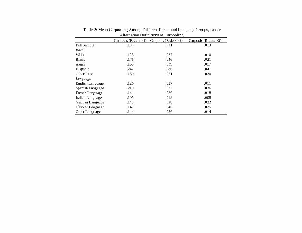
Carpools (Riders >1) Carpools (Riders >2) Carpools (Riders >3)Full Sample .134 .031 .013RaceWhite .123 .027 .010Black .176 .046 .021Asian .153 .039 .017Hispanic .242 .086 .041Other Race .189 .051 .020LanguageEnglish Language .126 .027 .011Spanish Language .219 .075 .036French Language .141 .036 .018Italian Language .105 .018 .008German Language .143 .038 .022Chinese Language .147 .046 .025Other Language .144 .036 .014

Table 2: Mean Carpooling Among Different Racial and Language Groups, Under Alternative Definitions of Carpooling

Excluded Instruments: 30 Terms Summarizing Racial Makeup of State of Birth in Year Born

Statistic White Black Asian HispanicPartial R2 0.0040 0.0045 0.0009 0.0043F (clustered by state and decade of birth) 13.78 11.01 11.65 9.89 p value 0.0000 0.0000 0.0000 0.0000

Number of Observations 436,262 436,262 436,262 436,262Number of State-Decade Clusters 247 247 247 247See Text for Further Explanation

Endogenous Regressor: Fraction of PUMA in 1990 Which Is:

Table 3: First Stage Diagnostics

(1) (2)Carpools: Riders >1 Carpools: Riders >2

Age 18-22 0.0471 0.0049(0.0029) (0.0015)

Age 23-30 0.0291 0.0034(0.0020) (0.0010)

Age 31-45 0.0135 -0.0013(0.0019) (0.0009)

Age 46-55 0.0163 0.0020(0.0019) (0.0009)

Married 0.0148 0.0016(0.0016) (0.0008)

In School -0.0254 -0.0073(0.0017) (0.0009)

Bachelor's Degree -0.0257 -0.0071(0.0012) (0.0006)

Grad School + -0.0180 -0.0038(0.0020) (0.0010)

Log Earnings 0.0365 -0.0003(0.0059) (0.0033)

Log Earnings Squared -0.0030 -0.0002(0.0003) (0.0002)

Homeowner -0.0183 -0.0056(0.0014) (0.0008)

Urban 0.0014 0.0046(0.0017) (0.0009)

Small Lot 0.0007 0.0002(0.0013) (0.0007)

City -0.0032 -0.0007(0.0024) (0.0012)

Work In Same Puma -0.0164 -0.0116(0.0015) (0.0009)

Log Travel Time 0.0405 0.0188(0.0009) (0.0006)

1 Car 0.0302 -0.0133(0.0038) (0.0024)

2 Cars -0.0470 -0.0307(0.0042) (0.0025)

3 Cars -0.0591 -0.0337(0.0043) (0.0026)

4+ Cars -0.0722 -0.0409(0.0046) (0.0027)

Log Population Density -0.0027 -0.0010(0.0009) (0.0005)

Percent Bachelor's Degree 0.0451 0.0057(0.0218) (0.0117)

Percent Grad School + 0.2706 0.0615(0.0764) (0.0427)

Log Mean Travel Time -0.0228 -0.0017(0.0063) (0.0033)

Child Dummies Yes YesHousehold Size Dummies Yes YesOccupational Controls Yes YesIndustry Controls Yes YesObservations 496280 496280PUMAs 1726 1726R-squared 0.0609 0.0386Data drawn from merged IPUMS Census Sample. Controls not shown included in Appendix Table 2.All regressions include controls for state fixed effects.Standard errors adjusted for clustering by PUMA

Table 4: Linear Probability Estimate of Carpooling Determinants Among Working Men Age 164 From Merged IPUMS-STF3 Data

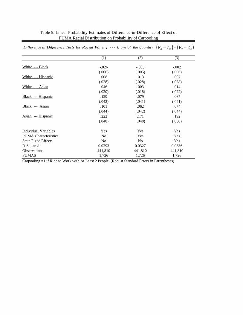
(1) (2) (3)

-.026 -.005 -.002(.006) (.005) (.006).008 .013 .007

(.028) (.028) (.028).046 .003 .014

(.020) (.018) (.022).129 .079 .067

(.042) (.041) (.041).101 .062 .074

(.044) (.042) (.044).222 .171 .192

(.048) (.048) (.050)

Individual Variables Yes Yes YesPUMA Characteristics No Yes YesState Fixed Effects No No YesR-Squared 0.0293 0.0327 0.0336Observations 441,810 441,810 441,810PUMAS 1,726 1,726 1,726Carpooling =1 if Ride to Work with At Least 2 People. (Robust Standard Errors in Parentheses)

Black --- Hispanic

Black --- Asian

Asian --- Hispanic

Table 5: Linear Probability Estimates of Difference-in-Difference of Effect of PUMA Racial Distribution on Probability of Carpooling

White --- Black

White --- Hispanic

White --- Asian

( ) ( ) - - - jj jk kj kkDifference in Difference Tests for Racial Pairs j k are of the quantity γ γ γ γ− − −

(1) (2) (3)

.034 .363 .317(.108) (.136) (.114).738 .618 .438

(.196) (.244) (.263).005 -.066 -.116

(.116) (.099) (.094).899 .226 .142

(.703) (.637) (.387).526 1.024 .986

(1.130) (1.033) (.589)1.095 1.178 1.607(.487) (.518) (.681)

Individual Variables Yes Yes YesPUMA Characteristics No Yes YesState Fixed Effects No No YesR-Squared N/A N/A N/AObservations 436,262 436,262 436,262PUMAS 1,726 1,726 1,726State-Decade Clusters 247 247 247Carpooling =1 if Ride to Work with At Least 2 People.Standard errors clustered by state and decade of birth

Black --- Hispanic

Black --- Asian

Asian --- Hispanic

Table 6: TSLS Linear Probability Estimates of Difference-in-Difference of Effect of PUMA Racial Distribution on Probability of Carpooling

White --- Black

White --- Hispanic

White --- Asian

( ) ( ) - - - jj jk kj kkDifference in Difference Tests for Racial Pairs j k are of the quantity γ γ γ γ− − −

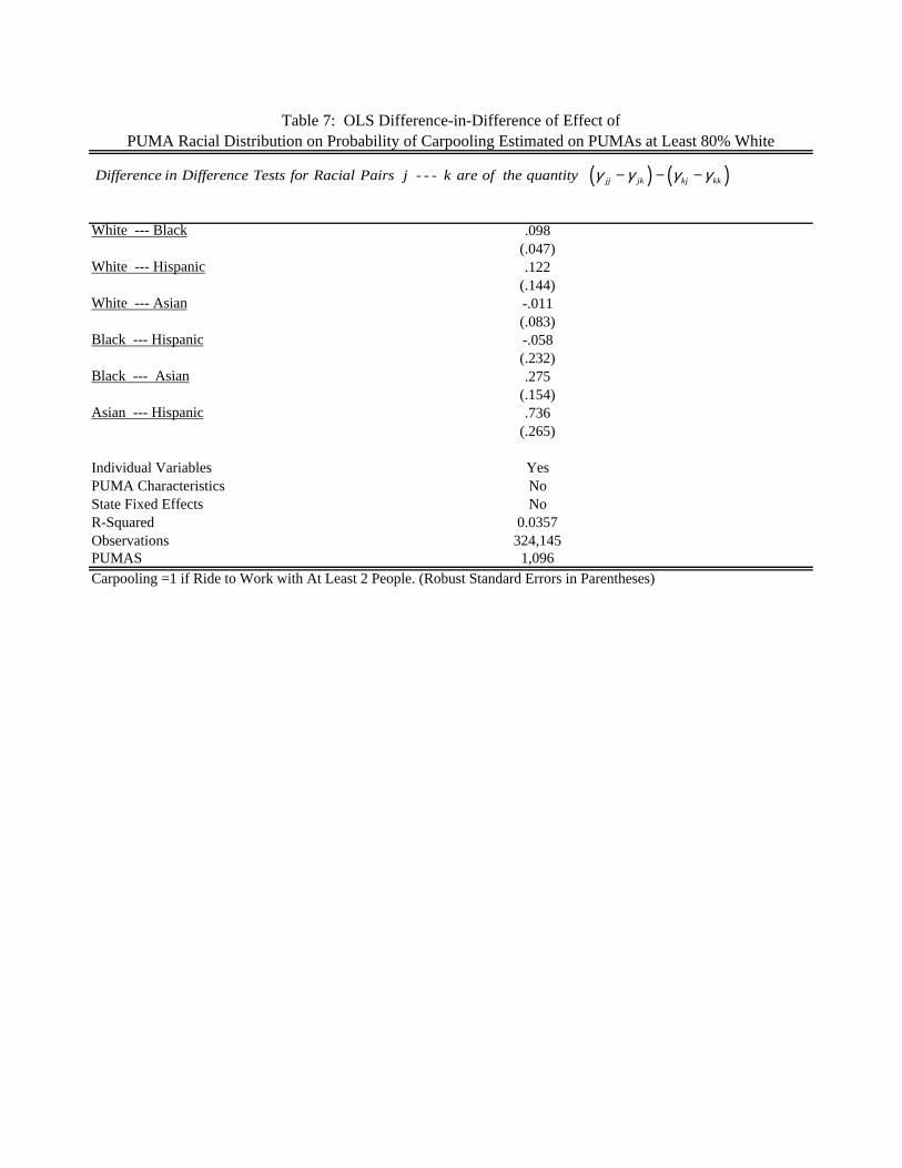
.098(.047).122

(.144)-.011(.083)-.058(.232).275

(.154).736

(.265)

Individual Variables YesPUMA Characteristics NoState Fixed Effects NoR-Squared 0.0357Observations 324,145PUMAS 1,096Carpooling =1 if Ride to Work with At Least 2 People. (Robust Standard Errors in Parentheses)

Black --- Hispanic

Black --- Asian

Asian --- Hispanic

Table 7: OLS Difference-in-Difference of Effect of PUMA Racial Distribution on Probability of Carpooling Estimated on PUMAs at Least 80% White

White --- Black

White --- Hispanic

White --- Asian

( ) ( ) - - - jj jk kj kkDifference in Difference Tests for Racial Pairs j k are of the quantity γ γ γ γ− − −

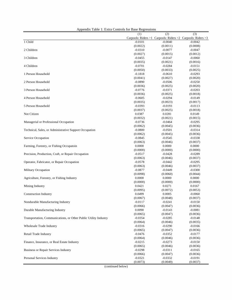
(1) (2) (3)Carpools: Riders >1 Carpools: Riders >2 Carpools: Riders >3

1 Child -0.0101 -0.0040 -0.0042(0.0022) (0.0011) (0.0008)

2 Children -0.0310 -0.0077 -0.0047(0.0027) (0.0015) (0.0012)

3 Children -0.0455 -0.0147 -0.0060(0.0035) (0.0021) (0.0016)

4 Children -0.0701 -0.0284 -0.0151(0.0050) (0.0033) (0.0025)

1 Person Household -0.1818 -0.0610 -0.0293(0.0041) (0.0027) (0.0020)

2 Person Household -0.0890 -0.0506 -0.0250(0.0036) (0.0025) (0.0020)

3 Person Household -0.0776 -0.0371 -0.0203(0.0036) (0.0025) (0.0018)

4 Person Household -0.0605 -0.0294 -0.0149(0.0035) (0.0023) (0.0017)

5 Person Household -0.0393 -0.0193 -0.0113(0.0037) (0.0025) (0.0018)

Not Citizen 0.0387 0.0281 0.0149(0.0032) (0.0021) (0.0015)

Managerial or Professional Occupation -0.0736 -0.0464 -0.0295(0.0062) (0.0045) (0.0036)

Technical, Sales, or Administrative Support Occupation -0.0800 -0.0501 -0.0314(0.0062) (0.0045) (0.0036)

Service Occupation -0.0845 -0.0545 -0.0338(0.0063) (0.0046) (0.0037)

Farming, Forestry, or Fishing Occupatoin 0.0000 0.0000 0.0000(0.0000) (0.0000) (0.0000)

Precision, Production, Craft, or Repair Occupation -0.0517 -0.0428 -0.0289(0.0063) (0.0046) (0.0037)

Operator, Fabricator, or Repair Occupation -0.0578 -0.0442 -0.0295(0.0063) (0.0046) (0.0037)

Military Occupation -0.0877 -0.0449 -0.0300(0.0098) (0.0060) (0.0044)

Agriculture, Forestry, or Fishing Industry 0.0000 0.0000 0.0000(0.0000) (0.0000) (0.0000)

Mining Industry 0.0421 0.0271 0.0167(0.0095) (0.0072) (0.0053)

Construction Industry 0.0499 0.0005 -0.0060(0.0067) (0.0048) (0.0037)

Nondurable Manufacturing Industry -0.0117 -0.0241 -0.0150(0.0066) (0.0047) (0.0036)

Durable Manufacturing Industry 0.0090 -0.0143 -0.0081(0.0065) (0.0047) (0.0036)

Transportation, Communications, or Other Public Utility Industry -0.0354 -0.0285 -0.0148(0.0064) (0.0046) (0.0035)

Wholesale Trade Industry -0.0316 -0.0290 -0.0166(0.0065) (0.0047) (0.0036)

Retail Trade Industry -0.0476 -0.0352 -0.0177(0.0064) (0.0046) (0.0036)

Finance, Insurance, or Real Estate Industry -0.0215 -0.0273 -0.0150(0.0065) (0.0046) (0.0036)

Business or Repair Services Industry -0.0298 -0.0311 -0.0165(0.0066) (0.0047) (0.0036)

Personal Services Industry -0.0321 -0.0332 -0.0191(0.0073) (0.0049) (0.0037)

Appendix Table 1: Extra Controls for Base Regressions

(continued below)

(1) (2) (3)Riders >1 Riders >2 Riders >3

Entertainment or Recreation Services Industry -0.0253 -0.0309 -0.0165(0.0074) (0.0050) (0.0038)

Professional or Related Services Industry 0.0004 -0.0202 -0.0115(0.0065) (0.0046) (0.0036)

Public Administration Industry 0.0074 -0.0125 -0.0066(0.0067) (0.0047) (0.0036)

Military Industry -0.0227 -0.0264 -0.0129(0.0080) (0.0056) (0.0041)

Percent Agriculture, Forestry, and Fishing Industry 0.2126 0.2329 0.1749(0.0537) (0.0326) (0.0237)

Percent Mining Industry 1.0268 0.7824 0.3917(0.2886) (0.1839) (0.1573)

Percent Construction Industry 1.0712 0.7420 0.3596(0.2913) (0.1904) (0.1626)

Percent Nondurables Manufacturing Industry 0.8279 0.6765 0.3510(0.2853) (0.1807) (0.1540)

Percent Durables Manufacturing Industry 0.8471 0.6328 0.3167(0.2852) (0.1795) (0.1536)

Percent Transportation Industry 0.7230 0.6026 0.2812(0.2935) (0.1860) (0.1586)

Percent Communications Industry 1.3499 0.7666 0.3477(0.3027) (0.1874) (0.1590)

Percent Wholesale Trade Industry 0.8520 0.5820 0.2663(0.3041) (0.1967) (0.1677)

Percent Retail Trade Industry 0.9231 0.7041 0.3439(0.2868) (0.1813) (0.1550)

Percent Finance, Insurance, and Real Estate Industry 0.9045 0.6936 0.3236(0.2933) (0.1889) (0.1598)

Percent Business & Repair Services Industry 0.8545 0.7080 0.3379(0.3028) (0.1860) (0.1541)

Percent Personal Services Industry 0.9385 0.5658 0.2802(0.2988) (0.1841) (0.1572)

Percent Entertainment & Recreation Services Industry 1.0287 0.6763 0.3174(0.2970) (0.1844) (0.1558)

Percent Health Services Industry 0.9982 0.7013 0.3288(0.2869) (0.1784) (0.1513)

Percent Educational Services Industry 0.9274 0.6729 0.3204(0.2894) (0.1814) (0.1548)

Percent Other Professional & Related Specialties Industry 0.6931 0.5778 0.2961(0.3020) (0.1852) (0.1583)

Percent Public Administration Industry 1.1921 0.7892 0.3889(0.2866) (0.1826) (0.1559)

Percent Executive, Administrative, and Managerial Occupation -0.9652 -0.6502 -0.3261(0.2984) (0.1909) (0.1587)

Percent Professional Specialty Occupation -1.0408 -0.6765 -0.3175(0.2934) (0.1800) (0.1540)

Percent Technicians & Related Support Occupation -0.7169 -0.6065 -0.2750(0.3094) (0.1869) (0.1576)

Percent Sales Occupation -0.8809 -0.6873 -0.2966(0.2929) (0.1871) (0.1595)

Percent Administrative Support Occupation -1.0054 -0.7489 -0.3448(0.2900) (0.1854) (0.1580)

Percent Private Services Occupation -1.2490 -0.8297 -0.3605(0.4052) (0.2350) (0.1714)

Percent Protective Services Occupation -0.4779 -0.5220 -0.2786(0.3079) (0.1878) (0.1538)

Appendix Table 1: Extra Controls for Base Regressions (continued)

(continued below)

(1) (2) (3)Riders >1 Riders >2 Riders >3

Percent Other Services Occupation -1.0448 -0.6759 -0.3254(0.2941) (0.1806) (0.1522)

Percent Farming, Forestry, and Fishing Occupation 0.0000 0.0000 0.0000(0.0000) (0.0000) (0.0000)

Percent Precision Production, Craft, & Repair Occupation -0.8071 -0.6736 -0.3370(0.2837) (0.1799) (0.1524)

Percent Machine Operators, Assemblers, & Inspectors Occupation -0.6588 -0.6119 -0.3203(0.2887) (0.1800) (0.1525)

Percent Transportation & Material Moving Occupation -1.0788 -0.8041 -0.3874(0.3235) (0.2023) (0.1704)

Percent Handlers, Equipment Cleaners, Helpers & Laborers Occupation -0.4471 -0.3264 -0.1255(0.3222) (0.2045) (0.1696)

Observations 496280 496280 496280PUMAs 1726 1726 1726R-squared 0.0609 0.0386 0.0234All regressions include controls for state fixed effects.Standard errors adjusted for clustering by PUMA

Appendix Table 1: Extra Controls for Base Regressions (continued)

Full SampleShare of PUMA: Variance Variance Variance Ratio Variance Variance RatioRaceWhite 0.04111 0.00284 0.07 0.19600 4.77Black 0.03119 0.00175 0.06 0.05006 1.60Asian 0.00383 0.00039 0.10 0.00905 2.36Hispanic 0.00530 0.00057 0.11 0.01080 2.04Other 0.00075 0.00020 0.26 0.00171 2.27

Appendix Table 2: Variance of (Percent Puma Given Type), by Puma in Full Sample, Restricted Sample, and Dropped Sample

Percent PUMA White > 80% Percent PUMA White < 80%

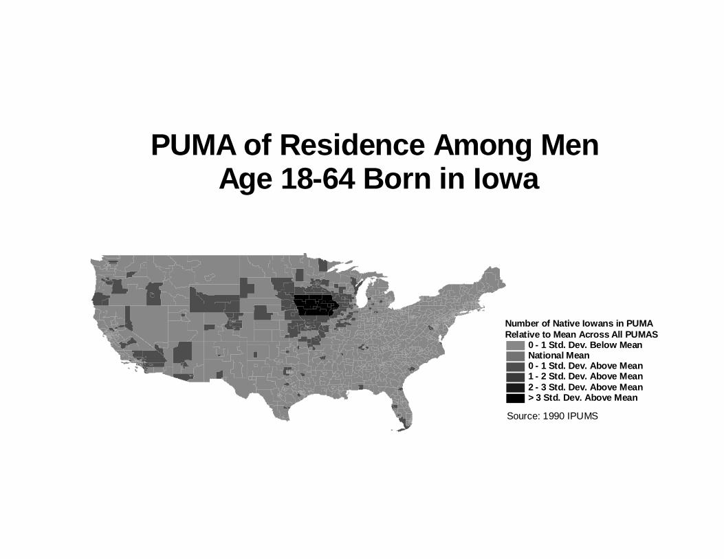
PUMA of Residence Among Men Age 18-64 Born in Iowa

Number of Native Iowans in PUMA Relative to Mean Across All PUMAS

0 - 1 Std. Dev. Below MeanNational Mean0 - 1 Std. Dev. Above Mean1 - 2 Std. Dev. Above Mean2 - 3 Std. Dev. Above Mean> 3 Std. Dev. Above Mean

Source: 1990 IPUMS

PUMA of Residence Among Men Age 18-64 Born in Massachusetts

Number Born in Massachusetts in PUMA Relative to Mean Across All PUMAS

0 - 1 Std. Dev. Below MeanNational Mean0 - 1 Std. Dev. Above Mean1 - 2 Std. Dev. Above Mean2 - 3 Std. Dev. Above Mean> 3 Std. Dev. Above Mean

Source: 1990 IPUMS

PUMA of Residence Among Men Age 18-64 Born in California

Number of Native Californians in PUMA Relative to Mean Across All PUMAS

0 - 1 Std. Dev. Below MeanNational Mean0 - 1 Std. Dev. Above Mean1 - 2 Std. Dev. Above Mean2 - 3 Std. Dev. Above Mean> 3 Std. Dev. Above Mean

Source: 1990 IPUMS

PUMA of Residence Among Men Age 18-64 Born in Alabama

Number Born in Alabama in PUMA Relative to Mean Across All PUMAS

0 - 1 Std. Dev. Below MeanNational Mean0 - 1 Std. Dev. Above Mean1 - 2 Std. Dev. Above Mean2 - 3 Std. Dev. Above Mean> 3 Std. Dev. Above Mean

Source: 1990 IPUMS

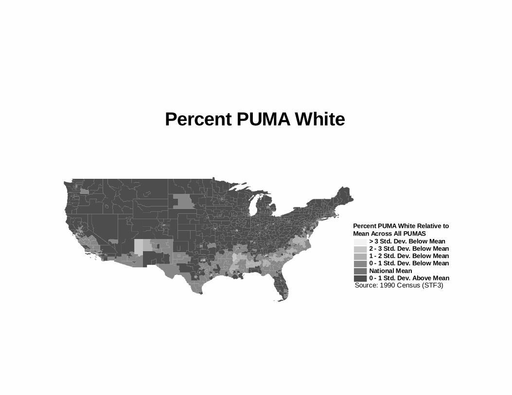
Percent PUMA White

Percent PUMA White Relative to Mean Across All PUMAS

> 3 Std. Dev. Below Mean2 - 3 Std. Dev. Below Mean1 - 2 Std. Dev. Below Mean0 - 1 Std. Dev. Below MeanNational Mean0 - 1 Std. Dev. Above Mean

Source: 1990 Census (STF3)

Percent PUMA Black

Percent PUMA Black Relative to Mean Across All PUMAS

0 - 1 Std. Dev. Below MeanNational Mean0 - 1 Std. Dev. Above Mean1 - 2 Std. Dev. Above Mean2 - 3 Std. Dev. Above Mean> 3 Std. Dev. Above Mean

Source: 1990 Census (STF3)

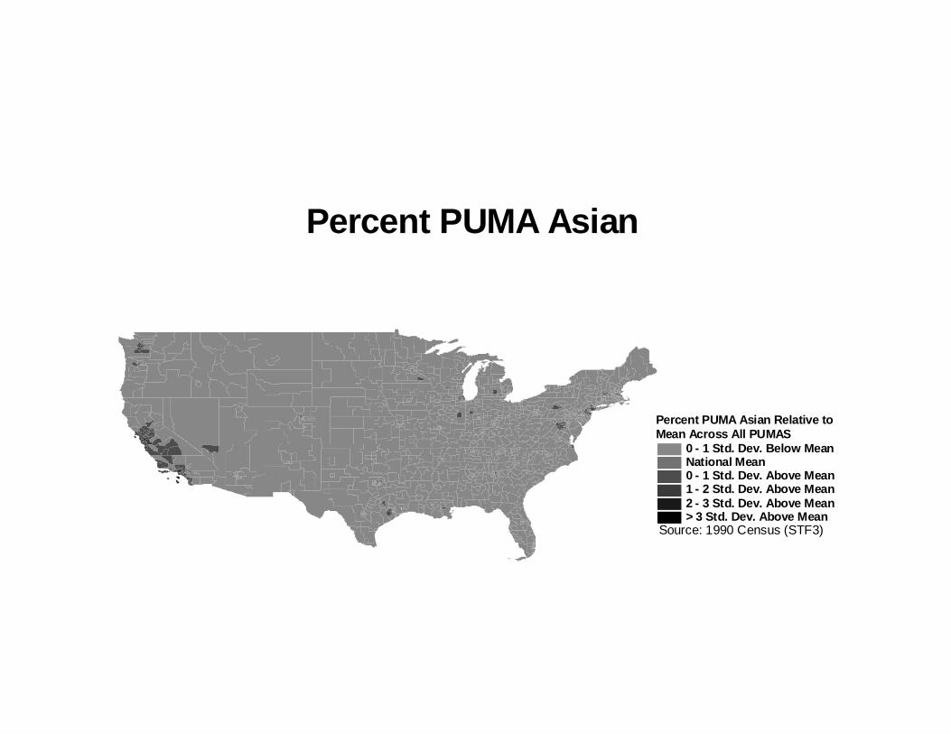
Percent PUMA Asian

Percent PUMA Asian Relative to Mean Across All PUMAS

0 - 1 Std. Dev. Below MeanNational Mean0 - 1 Std. Dev. Above Mean1 - 2 Std. Dev. Above Mean2 - 3 Std. Dev. Above Mean> 3 Std. Dev. Above Mean

Source: 1990 Census (STF3)

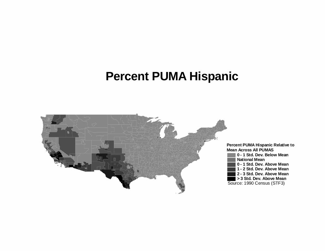
Percent PUMA Hispanic

Percent PUMA Hispanic Relative to Mean Across All PUMAS

0 - 1 Std. Dev. Below MeanNational Mean0 - 1 Std. Dev. Above Mean1 - 2 Std. Dev. Above Mean2 - 3 Std. Dev. Above Mean> 3 Std. Dev. Above Mean

Source: 1990 Census (STF3)