NBER WORKING PAPER SERIES

MENU COSTS AND PHILLIPS CURVES

Mikhail GolosovRobert E. Lucas, Jr.

Working Paper 10187http://www.nber.org/papers/w10187

NATIONAL BUREAU OF ECONOMIC RESEARCH1050 Massachusetts Avenue

Cambridge, MA 02138December 2003

We have benefitted from discussions with Ariel Burstein, Ricardo Caballero, V.V. Chari, Larry Christiano,Larry Jones, Boyan Jovanovic, Patrick Kehoe, Timothy Kehoe, Bob King, Pete Klenow, Oleksiy Kryvtsov,Ellen McGrattan, Thomas Philippon, Thomas Sargent, Nancy Stokey, Julia Thomas, and Aleh Tsyvinski.Participants in seminars at Chicago, Minnesota, the Federal Reserve Bank of Minneapolis, the CEPRconference “The Phillips Curve Revisited” and the NBER Economic Fluctuations and Growth meetingprovided helpful criticism. The views expressed herein are those of the authors and not necessarily those ofthe National Bureau of Economic Research.

©2003 by Mikhail Golosov and Robert E. Lucas, Jr. All rights reserved. Short sections of text, not to exceedtwo paragraphs, may be quoted without explicit permission provided that full credit, including © notice, isgiven to the source.

Menu Costs and Phillips CurvesMikhail Golosov and Robert E. Lucas, Jr.NBER Working Paper No. 10187December 2003JEL No. E0

ABSTRACT

This paper develops a model of a monetary economy in which individual firms are subject to

idiosyncratic productivity shocks as well as general inflation. Sellers can change price only by

incurring a real “menu cost.” We calibrate this cost and the variance and autocorrelation of the

idiosyncratic shock using a new U.S. data set of individual prices due to Klenow and Kryvtsov. The

prediction of the calibrated model for the effects of high inflation on the frequency of price changes

accords well with the Israeli evidence obtained by Lach and Tsiddon. The model is also used to

conduct numerical experiments on the economy’s response to credible and incredible disinflations

and other shocks. In none of the simulations we conducted did monetary shocks induce large or

persistent real responses.

Mikhail GolosovResearch DepartmentFederal Reserve Bank of MinneapolisP.O. Box 291Minneapolis, MN 55480-0291golosov@econ.umn.edu

Robert E. Lucas, Jr.Department of EconomicsUniversity of Chicago1126 East 59th StreetChicago, IL 60637and NBERrelucas@uchicago.edu

1. Introduction

As an explanation for some of the apparent real effects of inflations, menu costs–

real resources required to change nominal prices–have an evident appeal. Such costs

are by definition a source of nominal “rigidity” or “stickiness,” and lump-sum costs

have the added attraction that action will be taken infrequently and only in response

to changes that are viewed as permanent. Thus menu cost models are consistent with

the fact that even large disinflations have small real effects if credibly carried out.1

Finally, and not least, menu costs are really there: The fact that many individual

goods prices remain fixed for weeks or months in the face of continuously changing

demand and supply conditions testifies conclusively to the existence of a fixed cost of

repricing.

Granting these qualitative observations, it would be good to know how large

the real effects of price stickiness induced by menu costs might be. Phillips curves

estimated from aggregate data provide one source of information, but such estimates

are notoriously unstable and can be given many different interpretations. In this

paper, we calibrate a menu cost model using a new data set on prices, based on

Bureau of Labor Statistics surveys, assembled and described by Bils and Klenow

(2002) and Klenow and Kryvtsov (2003). This estimation makes use of both cross-

section and time series evidence on the prices of narrowly-defined individual goods,

1Sargent (1986).

2

and summary statistics on the frequency of individual price changes. The calibrated

model is then used to carry out several numerical experiments involving the economy’s

responses to specified changes in the overall inflation rate.

A distinctive feature of the model we use is the assumption that each seller is

subject to two shocks that affect its pricing decision: an aggregate shock, reflecting

economy-wide inflation, and an idiosyncratic shock, reflecting good-specific changes in

technology or preferences. In such a world, an observed price change may be triggered

by either kind of shock, or a mix of the two, and the pricing decisions of individual

sellers will not be synchronized. Observations on aggregates must be interpreted as

averages over a more complex microeconomic reality. In the next section we define an

equilibrium in a model with this feature, in which inflation is defined by changes in

an economy-wide nominal wage rate that follows an exogenously given random walk,

with constant drift and variance.

The definition we propose in Section 2 is a little too general to permit us to

calculate or characterize equilibria, and the rest of the paper examines a series of

special cases and approximations. In Sections 3 and 4, we specialize to the case

where the inflation rate is constant and the idiosyncratic shock is mean-reverting.

In this version of the model, suitably normalized prices follow a continuous time

Markov process that has an invariant distribution. We derive the Bellman equation for

individual firms in this context. We describe a discrete-time model that can provide an

arbitrarily good approximation to the continuous-time model, and for which solutions

are inexpensive to compute. We use the approximate model to compute the optimal

pricing behavior of firms.

This model predicts the fraction of prices that are changed per month, the key

parameter in the widely-applied model of Calvo (1983). We use the model to examine

the sensitivity of this fraction to changes in inflationary behavior. Then we compare

the predictions of the model, as estimated from data from the low-inflation U.S.

3

economy of 1988-97, to Lach and Tsiddon’s (1992) evidence on the frequency of price

changes during the Israeli inflations of 1978-1979 and 1981-82. The predictions of the

model are surprisingly accurate.

One of the most striking predictions of our model is that idiosyncratic shocks

account for most of the price adjustments in the U.S. In the U.S. data, more than

20 percent of all consumer prices are adjusted each month, and the average size

of the change in the individual prices that are adjusted is much larger than the

expected inflation between adjustments: The average price is changed once every five

months, and the average inflation in the U.S. over five months is roughly one percent,

while prices are changed on average by as much as 10 percent. These observations

suggest that idiosyncratic shocks–shocks to productivity or demand–are responsible

for most of the price changes. Our simulations confirm this intuition. When the

idiosyncratic shocks in the model are shut down, the frequency of price adjustments

is roughly unchanged in high inflationary environments but it is much reduced when

inflation is low.

Even though idiosyncratic shocks cause most of the price adjustments, new prices

reflect both firm-level and aggregate shocks. Thus even a small inflationary shock, one

which is not sufficient to lead to a price change on its own, is quickly reflected in new

prices as firms react to other shocks. This makes it difficult to obtain a large degree

of persistence for monetary shocks in our menu cost environment. Our simulations

also show this effect very clearly.

Although the simulated economy fits observed pricing behavior well, it exhibits

very small real effects of monetary instability. Simulated time series with realistic

monetary variability have a variance of aggregate output that is ten times lower than

that observed in the recent U.S. data. The estimated Phillips curve is also very flat:

A one percentage point reduction in inflation rate depresses output by only 0.05 of

one percent. Thus money appears nearly neutral: The effects of inflation shocks on

4

aggregate production and employment, as we estimate them, are small and transient.

Similar results hold for different policy experiments. For a credible disinflation–

we use an immediate reduction in the rate of wage inflation from 15 to one percent

per quarter–there are essentially no real effects, consistent with Sargent’s (1986)

findings. But even when the disinflation is carried out in a non-credible way, the

resulting decline in production never exceeds one percent of GDP. We summarize

these and other findings in more detail in a concluding section.

The model we describe in the next section builds on the original formulation of

the pricing problem of a single firm by Sheshinski and Weiss (1977), and on the long

literature of other papers that apply ( )-type inventory theory to pricing problems.2

It has proved difficult to situate these pricing models in equilibrium models, but

several precedents have been influential and valuable. Calvo (1983) leaves the fixed

cost in the background, assuming instead that a firm gets an option to re-price in any

period with a fixed probability that does not depend on its own state. By varying

this probability, any desired degree of price “stickiness” can be built into a model.

Caplin and Spulber (1987) considered equilibrium in an economy in which the money

supply always grows, the firm with the lowest price at any instant re-prices, and to

the top of the price distribution. They show that a rectangular distribution of firms

by their price levels is stationary, and that the distribution of prices relative to the

money supply is stationary and independent of the path of money. This was a striking

example of an economy with an extremely low re-pricing rate (in Calvo’s terms) that

would appear to an observer of aggregates to have no price stickiness at all. Further

developments can be found in Caplin and Leahy (1991) and elsewhere.

2Sheshinski and Weiss (1977) analyzed the pricing decision of an individual seller facing a deter-

ministic trend in the desired price level. Versions of this problem, many of them stochastic, have

been studied by Sheshinski and Weiss (1983), Frenkel and Jovanovic (1980), Chang (1999), Mankiw

(1985), and Stokey (2002).

5

Lach and Tsiddon (1992) look at individual price distributions in Israel, finding

them not to be rectangular and the changes not to be synchronized, even for firms

with the same initial price. They suggest that a successful model would need to have

idiosyncratic shocks as well as economy-wide shocks. Dotsey, King, and Wolman

(1999) propose a monetary equilibrium model in which the synchronization of price

changes is broken by a transient, random shock to the menu cost itself: Firms that

draw high cost have an incentive to postpone re-pricing. They explore a number

of issues numerically using a log-linear approximation. Further developments are

described in Willis (2000) and Burstein (2002).

The model developed and applied below shares both its two-shock character

and its use of numerical methods with Dotsey, King, and Wolman (1999) and their

successors. In the Dotsey, King, and Wolman (1999) model, the idiosyncratic shock

affects an individual firm’s menu cost and thus influences which firms will re-price at

a given time. All firms that do re-price move to the same new price. In our model,

in contrast, the idiosyncratic shock affects productivity, and affects both which firms

will re-price and the new prices of those who do. This feature allows us to capture

observable heterogeneity in individual pricing behavior: Prices for some goods are

increased for some and decreased for others, and the size of price adjustment is not

closely related to the expected inflation rate at the time price is adjusted.

The paper is organized as follows. In Section 2 we lay out the general model.

Section 3 containts the benchmark specification of the model with constant inflation

rate. Section 4 describes the data we used and the calibation procedure. Section 5

then describes the results of some simulations of disinflations, conducted using the

model of Section 3. We compare credible and non-credible disinflations. Section

6 calculates some impulse-response functions. Section 7 re-introduces a stochastic

shock to the inflation rate, and proposes an approximation to the firm’s pricing policy.

This approximation is then used to examine the behavior of Phillips curves, in the

6

sense of correlations between inflation rates and levels of production and employment.

Estimates of the fraction of the variability in these variables that can be accounted

for by monetary shocks in the presence of menu costs are also provided.

2. A Model of Monetary Equilibrium

The theory that we calibrate and simulate in this paper is a Bellman equation

for a single, price-setting firm that hires labor at a given nominal wage, produces a

consumption good with a stochastically varying technology, and sets product price

subject to a menu cost of re-pricing. We situate our model of a firm in a model of a

monetary economy so as to be able to relate its predictions to aggregative evidence.

In this economy, there is a continuum of infinitely lived households, each of which

consumes a continuum of goods. A Spence-Dixit-Stiglitz3 utility function is used to

aggregate across goods to form current period utility. Each household also supplies

labor on a competitive labor market. Firms hire labor, used to produce the consump-

tion good and to re-set nominal prices for the good, and sell goods to consumers.

Each firm produces only one of the continuum of consumption goods.

The economy is subject to two kinds of shocks: a monetary shock, which we

summarize in the implied money wage rate, and a firm-specific productivity shock

. The log of the nominal wage, = log(), is assumed to follow a Brownian

motion with drift parameter and variance 2,

= + , (2.1)

where denotes a standard Brownian motion with zero drift and unit variance.

We think of the behavior of the money wage as ultimately being determined by the

behavior of the money supply, but this connection will not be modeled and the only

explicit role of dollars in the theory is as a unit of account. In the absence of the real

3Spence (1976) and Dixit-Stiglitz (1977).

7

menu costs associated with changing prices, the evolution of would have no effect

on resource allocation.

There are also firm-specific productivity shocks , which are assumed to be

independent across firms We assume that = log() follows a mean-reverting

Ornstein-Uhlenbeck process:

= − + , 0 (2.2)

where is a standard Brownian motion with zero drift and unit variance, distributed

independently of .

Equilibrium prices and quantities will be modeled as stochastic processes, defined

in terms of an initial joint distribution 0( ) of firms by their inherited price

and productivity level and by the evolution of the exogenous processes and

Specifically, each firm chooses a pricing strategy , a stochastic processes thattakes the form of a right-continuous step function whose date value depends on the

histories of its own productivity shocks 0 and of the nominal wage shocks 04

The strategy that a firm chooses will also depend on its inherited initial price

0. When we want to emphasize this dependence we write (0)For given firm behavior (0), the initial joint distribution of (0 0), the

initial wage 0 and the probabilities implied by (2.1) and (2.2), induce a family of

probability measures for the prices facing consumers at all dates . For any Borel

set ⊂ R2,

() =ZPr((0) )() ∈ | 00(0 0) (2.3)

There is also a capital market, in which consumers trade contingent claims to

the monetary unit. We adopt the convention that

·Z ∞0

¸

4That is, the process is adapted to the filtration generated by (See, for example,Stokey (2002), ch. 1.)

8

is the value at date 0 of a dollar earnings stream ∞0 , also a stochastic processdefined in terms of Thus must be multiplied by the appropriate probabilities

to obtain the Arrow-Debreu prices.

We next describe the decision problem of consumers in this environment. At

each date , each household buys from every seller, and each seller is characterized by

a pair ( ) distributed according to the measure ( ). The household chooses

a buying strategy (·), where ( ) is the number of units of the consumption

good that it buys from a seller who charges price after the shock history 0 hasoccurred. It also chooses a labor supply strategy , where is the units of laborsupplied after the shock history 0 has occurred. The values ( ) and also

depend on the initial price distribution 0( )

For any buying strategy ( ) define as the Spence-Dixit-Stiglitz consumption

aggregate

=·Z

( )1−1( )

¸(−1) (2.4)

The corresponding current period utility is assumed to be

1

1− 1−

Preferences over time are

"Z ∞0

−Ã

1

1− 1− −

!

# (2.5)

The operator (·) is defined by the shock processes (2.1) and (2.2).We write the consumer’s budget constraint as

·Z ∞0

µZ( )( )− −Π

¶¸≤ 0 (2.6)

where Π is profit income, obtained from the household’s holdings of a fully diversified

portfolio of claims on the individual firms. The household chooses buying and labor

supply strategies (·) and so as to maximize (2.5), subject to (2.6), taking , and as given.

9

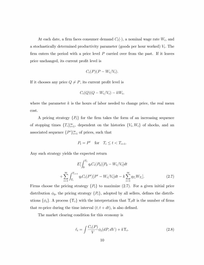
At each date, a firm faces consumer demand (·), a nominal wage rate , and

a stochastically determined productivity parameter (goods per hour worked) The

firm enters the period with a price level carried over from the past. If it leaves

price unchanged, its current profit level is

( )( −)

If it chooses any price 6= , its current profit level is

()(−)−

where the parameter is the hours of labor needed to change price, the real menu

cost.

A pricing strategy for the firm takes the form of an increasing sequence

of stopping times ∞=1, dependent on the histories of shocks, and anassociated sequence ∞=1 of prices, such that

= for ≤ ! +1

Any such strategy yields the expected return

[Z 1

0(0)[0 −]

+∞X=1

Z +1

()[ −]−

∞X=1

] (2.7)

Firms choose the pricing strategy to maximize (2.7). For a given initial pricedistribution 0, the pricing strategy , adopted by all sellers, defines the distrib-utions A process Υ with the interpretation that Υ is the number of firms

that re-price during the time interval ( + ), is also defined.

The market clearing condition for this economy is

=Z ( )

( ) + Υ (2.8)

10

The equality of goods consumed and goods produced is incorporated in (2.7). There

is no money market to clear because money does not appear as a good in the model:

It is just a unit of account.

The consumer side of the model is familiar. We will use the first-order conditions

for consumers to reformulate the firms’ problems, and then turn to the study of the

latter. The first-order conditions for the consumer include

−−

·Z( )

1−1( )¸1(−1)

( )−1 = " (2.9)

where the multiplier " does not depend on time, and

− = " (2.10)

Eliminating the multiplier between (2.9) and (2.10) and simplifying using (2.4) yields

−+1 ( )

−1 =

Solving for ( ), we obtain the demand function facing each firm:

( ) = 1−

µ

¶− (2.11)

Applying the natural normalization 0 = 1 to (2.10), we obtain

= −0

(2.12)

Inserting the solutions (2.11) and (2.12) from the consumer’s problem into the

firm’s objective function (2.7) then yields

0[Z 1

0−1−

µ0

¶−[0− 1

]

+∞X=1

Z +1

−1−

Ã

!−[

− 1

]− ∞X=1

−] (2.13)

We sum up in the following

11

Definition. Given an initial wage 0 and a joint price-shock distribution 0,

an equilibrium is a pricing strategy for firms, processes and for theconsumption aggregate and the price-shock distributions, and processes Υ and for the re-pricing frequencing and labor supply, such that (i) given maximizes (2.13), (ii) given satisfies (2.3), (iii) and satisfy (2.4),and such that Υ and satisfy (2.8), given and with ( ) given by (2.11).

In our view it is a limitation of this definition of equilibrium that inflation is

defined by the assumed exogenous behavior of nominal wages, and not indirectly by

the behavior of the money supply. We will not remedy this deficiency here, but a brief

digression on the issues involved in doing so may help in interpreting our results. Sup-

pose we were to introduce money# into the theory, treating it as a given stochastic

process, and motivate its use by adding real balances # as a second argument in

consumers’ utility function. Retaining additivity, the instantaneous utility flow could

then be written1

1− 1− + $(

#

)− (2.14)

say. An additional equilibrium condition would then be the equality of the marginal

rate of substitution between real balances and leisure to their relative price, or

$0(#

)1

=%

(2.15)

where % is the instantaneous nominal interest rate. The other equilibrium conditions

are not affected. The nominal interest rate in turn is essentially minus the rate of

change of the log of the price , given in (2.12), and is itself a stochastic process.

This familiar Fisherian connection between the level of real balances demanded and

the rate of change of the nominal wage means that, in general, nominal wages and

prices will not be proportional to the money supply along an equilibrium path.

12

But proportionality is a possibility. Suppose, for example, that $ is the log

function, so (2.15) becomes

#= %

Suppose further that the growth rate of money is constant at a rate . If the nominal

wage grows at the same rate, the instantaneous interest rate will be constant at &+

and the wage path

= (&+ )# (2.16)

will be an equilibrium.

These are assumptions on preferences and the money supply that exactly ra-

tionalize the calculations we report for constant wage growth in Sections 3 and 4.

Under many other assumptions on preferences and the role of money it would not be

difficult to “back out” the time series behavior of the money supply that would be

consistent with constant nominal wage growth, or with nominal wages following the

more general process (2.1). In our opinion, a money supply process constructed in

this way would be consistent with quantity-theoretic behavior similar, in a general

way, to (2.16). It would be informative, but also more difficult, to construct an equi-

librium wage process taking a money growth process as given. Both of these lines are

worth pursuing, but we will not do so in this paper.

Most previous work has been simplified by eliminating or avoiding the idiosyn-

cratic shocks, in our set-up, and focusing on aggregate inflation shocks only.We will initially go in the opposite direction, treating the special case in which the

variance 2 of the wage process is zero, so that the drift parameter is simply the

constant rate of wage inflation. In this situation, we will seek an invariant joint distri-

bution for prices and idiosyncratic shocks. In the next two sections, we formulate,

calibrate, and study a Bellman equation for this case of a stationary equilibrium with

constant inflation.

13

3. Stationary Equilibrium with Constant Inflation

Let the inflation rate be constant at , so that

= 0 (3.1)

Denote the value of the objective (2.13) of a firm in a stationary equilibrium that has

an inherited nominal price and exogenous shocks with current values ( ) by

Φ( ) In a stationary equilibrium, the consumption aggregate will be con-

stant at a value (say) and Φ will satisfy the Bellman equation

Φ( ) = max

[Z

0−1−

µ0

¶−[0

− 1

]

+− ·max[Φ( )− ]] (3.2)

It is convenient to restate (3.2) in terms of the logs: ( ) = ( ) and

to define a new state variable ' by

' = ( − (3.3)

Then between price changes the motion of ' is described by

' = − (3.4)

and the motion of follows (2.2). Then we seek a solution to (3.2) of the form

Φ( ) = Φ( ) = )((− ) = )(' ) where the function ) satisfies

)(' ) = max

"Z

0−Π(' ) + − max

0[)('0 ( ))− ]

# (3.5)

and where

Π(' ) = 1−()−[ − −] (3.6)

Note that the pricing policy ' that would maximize the profit function Π if there

were no menu cost would be

'∗ = log(*

*− 1)− (3.7)

14

We will study the problem (3.5) using a discrete-time and state approximation

to (2.2)–a Markov chain– following Kushner and Dupuis’s (2001) description of

finite-element methods. The approximate process () is assumed to take values on

the finite grid = − −2+−+ 0 + 2+ , so is the state space of the

Markov chain. For a given grid size + we specify a time interval ∆ and a transition

function , on

,( 0 ) = Pr ( +∆) = 0 | () =

in terms of the defining parameters ( ) of the original continuous-time process in

such a way that in the limit as + → 0 the conditional, local means and variances of

the original and approximate processes match. See the Appendix for details.

In the calculations reported below, we fix the grid size + and the set on which

the shocks values lie. Analogous to the definition of the set , we define a set

- = −' −2+−+ 0 + 2+ '

of possible ' values, so that states (' ) will be elements of = - × . Then we

approximate the continuous problem (3.5) with the discrete problem

.(' ) = maxΠ(' )∆+ −∆X0,( 0 | ).('∆ 0)

max0[Π('0 )∆ + −∆

X0,( 0 | ).('0∆ 0)]− (3.8)

Under the assumptions we have imposed there is a unique function . on that

satisfies (3.8).

To see the dynamic behavior implied by (3.8), it is useful to define some auxiliary

functions. Let

Ω( ) = max0[Π('0 )∆ + −∆

X0,( 0 | ).('0∆ 0)]

so Ω( ) is the value of discounted profit if a one-time, costless repricing can occur in

state Let /( ) be the price that attains the maximum. Then define the “inaction

15

region” 0( ) as

0( ) = ' ∈ - : .(' ) Ω( )−

(so that 0( ) is the set of ' = (− values at which it does not pay to re-price whenthe productivity shock is ). In our application, this region will be an open interval:

0( ) = (1( ) 2( ))

The policy function for (3.8) is thus the function 3 : → - defined by

3(' ) = ' if ' ∈ 0( )3(' ) = /( ) if ' ∈ 0( )

The (log) price in state (' ) is ( = + 3(' ).

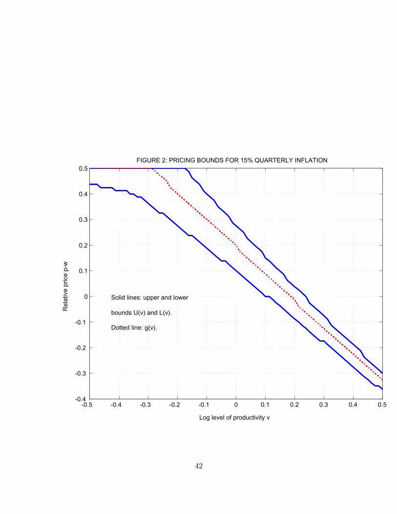
Figures 1 and 2 plot the three functions / 2 and 1 for quarterly inflation rates of

one and 15 percent. (These and other figures in this section are based on the baseline

parameter values given in Table 1 in Section 4.) These functions are decreasing: high

productivity shocks imply price decreases. Note that the inaction intervals 0( ) are

wider for low values: Getting prices “right” is more important when productivity

shocks–and hence quantities sold–are high. Note also the widening of the inaction

intervals as inflation increases. With high inflation, prices are changed often just to

keep up with general inflation, and pricing rules do not need to be as sensitive to

idiosyncratic productivity shocks. Higher inflation also induces a shift in the target

prices toward the upper boundary of the inaction region.

INSERT FIGURES 1 AND 2

Figures 3 and 4 illustrate simulated sample paths for the ideal price given in

(3.7), reflecting changes in relative productivity only. Figure 3 also plots the optimal

price path for the cost parameter = 0004 and the constant inflation rate = 01.

Figure 4 is the same in all respects, except that the cost parameter is decreased to

16

= 00004. One can see the way the step function for price tracks the ideal price,

and the fact that as the fixed cost decreases prices are changed more often and the

tracking gets better.

INSERT FIGURES 3, 4, AND 3a

Figure 3a, taken from Chevalier et al. (2000), shows the time series of actual

prices for Triscuits, based on scanner data from a Chicago supermarket chain. It is

instructive to compare this time series to those in our Figures 3 and 4. On Figure

3a, temporary sales are evident in the many times the Triscuit price is reduced for a

short time and returned to exactly the former price soon thereafter. Such patterns

are of course common to many price series. To obtain a good match between theory

and data, then, sales must either be removed from the data or added to the model.

As discussed below, we took the first course, made easier by the fact that the BLS

flags observations that they regard as sale prices. For us, then, the data have sale

observations removed. Do this with your eye on Figure 3a, and then compare it to

Figures 3 and 4.

The joint process (' ), where ' is controlled in the way we have just described,

has a unique ergodic set , given by

= (' ) ∈ : ' ∈ 0( )

(where the overbar means closure) and there is a unique invariant distribution 4(' )

on . It is impossible to pass the boundaries of the inaction region because whenever

the uncontrolled process would do so, price is revised to prevent this from occurring.

Figure 5 plots the implied density of the pricing error ' − '∗ for the two quarterly

inflation rates one percent and 15 percent that were used in Figures 1 and 2.

INSERT FIGURE 5

17

4. Data, Calibration, and a Test

Our basic model lacks many features that a business cycle model needs–it has

no capital and no aggregate shocks–but we drew on that literature for the values of

the preference parameters & , , and *. We used the annual discount rate & = 04,

the risk aversion parameter = 2 the elasticity of substitution parameter * = 7 and

the disutility of labor = 09 These & and values are conventional. The value of

* is related to the degree of monopoly power firms have: With * = 7, firm profits

are about 15 percent of GDP. The elasticity of substitution implies that a firm’s

mark-up–defined as the percent by which price exceeds marginal cost–is about 16

percent. Estimates of mark-ups typically fall in the 10-20 percent range, implying

values of * in the 6-10 percent range.5 Our results are not sensitive to changes in *

within that range. We interpreted our linear labor disutility as indivisible labor with

lotteries, following Hansen (1985). The value = 09 implies an average labor level

of 0.85.

For the menu cost parameter , the drift parameter and the two parameters 2

and that characterize the idiosyncratic productivity shocks, we used a new data set

on individual prices due to Klenow and Kryvtsov (2003). This price data set is based

on the BLS survey, and contains about 80,000 time series of individual price quotes

in 88 geographical locations. The series are either monthly or bimonthly, depending

on the location, for the years 1988-1997. The individual price quotes comprise 123

narrowly defined goods categories. The data set also provides the positive weights

,P

= 1 that are used to form the consumer price index from the individual

prices (called the CPI weights). We used the prices and weights for the New York

metropolitan area only to calibrate the parameters ( 2 2) and the fixed cost

5See, for example, Rotemberg and Woodford (1995) and Basu and Fernald (1997). It is not clear

to us, we should add, that the estimates reported in these studies are best interpreted as mark-ups

in the sense used in the text.

18

of the model described in the last two sections.

For calibrating the model under the assumption of a deterministic trend, we

imagine that the Klenow-Kryvtsov prices are generated by our model in the following

way. Prices for goods 5 = 1 6 are collected at the time intervals ∆. Denote these

prices by (() 5 = 1 6 For each good 5, let

(() = '() + ()

where for each () grows at the constant rate () is generated by (2.2), and

equilibrium prices are determined as described in the last two sections.6

We identify sample averages from the Klenow-Kryvtsov data with means taken

with respect to the invariant distribution 4(' ). If a seller begins a period in state

(' ), he immediately moves (re-prices) to (3(' ) ) so if 7 is any function on

its observed average value will beX

7 (3(' ) )4(' ) (4.1)

We first estimate the parameters ( 2) of the stochastic inflation process defined in

(2.1), and then turn to the calibration of ( 2,)

The weighted average price of goods (CPI) at time is

(() =X

(()

=X

['() + ()]

∼=X

'4(' ) + ()

where the second equality is a prediction of the theory, and the third replaces a sample

average with the population mean. Then since the first term on the right is constant

with respect to time, the model implies that

((+∆)− (() = (+∆)− () (4.2)6The BLS identifies some recorded prices as sale prices. We have replaced such observations with

the recorded price for the same good in the period before the sale. See Figure 3a.

19

Equation (4.2) suggests using the average and the variance of the differences of the

observed CPI series (() as estimates of ∆ and 2∆ respectively (though for

now we set 2 = 0)

The numbers in the first column of the first two rows of the table below report

these estimates. For the deterministic inflation version of the model, we set the

mean inflation rate equal to one percent and the standard deviation equal to zero,

as indicated in column 2. (Both means and standard deviations are expressed as

percentages.) The last three columns of the table indicate variations in the model’s

predictions under different choices for the parameters ( 2,) The first two rows are

not affected by these variations.

TABLE 1 : CALIBRATED PARAMETER VALUES

Baseline values: ( 2,) = (25 005 004)

Moment Data Model

Quarterly inflation rate .009 .01

S.d. of inflation .0374 0

Frequency of change .219 .231

Mean price increase .095 .075

S.d. of new prices .094 .1

= 015 2 = 0075 = 003

01 01 01

0 0 0

.227 .267 .261

.078 .084 .071

.133 .124 .101

Column (2) (“Model”) is based on the baseline values Columns

(3)-(5) are based on the same values, except for the changes indicated at

the head of each column.

To calibrate the three parameters ( 2,) we calculate three additional sample

moments that intuition suggests will convey information. The results are given in the

20

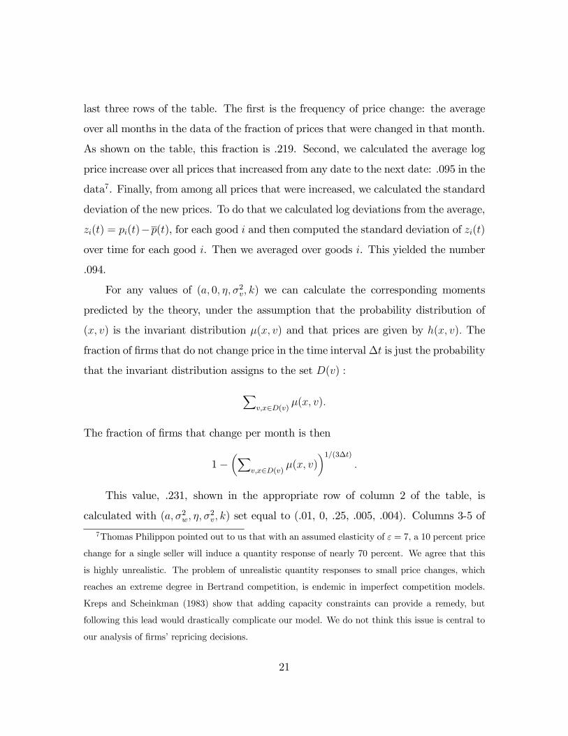
last three rows of the table. The first is the frequency of price change: the average

over all months in the data of the fraction of prices that were changed in that month.

As shown on the table, this fraction is .219. Second, we calculated the average log

price increase over all prices that increased from any date to the next date: .095 in the

data7. Finally, from among all prices that were increased, we calculated the standard

deviation of the new prices. To do that we calculated log deviations from the average,

8() = (()−((), for each good 5 and then computed the standard deviation of 8()over time for each good 5. Then we averaged over goods 5. This yielded the number

.094.

For any values of ( 0 2 ) we can calculate the corresponding moments

predicted by the theory, under the assumption that the probability distribution of

(' ) is the invariant distribution 4(' ) and that prices are given by +(' ) The

fraction of firms that do not change price in the time interval ∆ is just the probability

that the invariant distribution assigns to the set 0( ) :

X∈() 4(' )

The fraction of firms that change per month is then

1−µX

∈() 4(' )¶1(3∆)

This value, .231, shown in the appropriate row of column 2 of the table, is

calculated with ( 2 2 ) set equal to (.01, 0, .25, .005, .004). Columns 3-5 of

7Thomas Philippon pointed out to us that with an assumed elasticity of = 7, a 10 percent price

change for a single seller will induce a quantity response of nearly 70 percent. We agree that this

is highly unrealistic. The problem of unrealistic quantity responses to small price changes, which

reaches an extreme degree in Bertrand competition, is endemic in imperfect competition models.

Kreps and Scheinkman (1983) show that adding capacity constraints can provide a remedy, but

following this lead would drastically complicate our model. We do not think this issue is central to

our analysis of firms’ repricing decisions.

21

the table indicate how the calculated moments change as ( 2 ) are changed one at

a time from these benchmark values. That is, column 3 shows the computed statistics

when the parameter vector ( 2 2 ) = (01 0 25 005 004) is replaced by

(01 0 15 005 004) Thus the table shows that the frequency of price changes is

insensitive to changes in the rate of mean reversion in the idiosyncratic shock, that

it increases with the variance of these shocks, and that it decreases with increases in

the menu cost.

There are many studies that try to estimate or calibrate menu costs for particular

products. For example, Levy et al. (1997) estimate that the cost of changing prices

in supermarkets is about 0.7 percent of firms’ revenue. In our baseline model with

= 0004 menu costs are about 0.25 percent of revenues and 1.9 percent of profits.

The labor required to adjust prices is equal to 0.5 percent of overall employment.

We solved the model, calibrated as just described, for quarterly inflation rates

ranging from 0 to 20 percent, calculated the invariant distribution 4 in each case, and

calculated the fraction of firms that change price each month in this stationary equi-

librium. For comparison, we carried out the same calculations for the deterministic

Sheshinski-Weiss case where the variance of the idiosyncratic shocks is set equal to

zero. The results are shown in Figure 6. Also shown are three empirical observations:

the inflation-repricing pair (0.9,21.9) from the Klenow-Kryvtsov data, and the two

pairs (15,41) and (21,46) taken from the Lach-Tsiddon study of the Israeli inflations

in 1978-79 and 1981-82. The first pair lies exactly on the upper curve, reflecting the

fact that we used the Klenow-Kryvtsov data to calibrate our model. The model so

calibrated fits exactly the Israeli inflations, too. This is a genuine test of the theory,

carried out with evidence that is far out of sample.

Figure 6 also confirms the necessity of including idiosyncratic shocks if the model

is to fit the evidence from low inflation economies. As inflation rates are reduced, a

lot of “price stickiness” remains in the data. Of course, this evidence does not bear on

22

our interpretation of the idiosyncratic shocks as productivity differences, as opposed

to shifts in preferences, responses to inventory build-ups, or other factors.

INSERT FIGURE 6

The monthly re-pricing rates ranging from 22 to 46 percent shown on the figure

may be compared to Calvo’s (1983) assumption that the re-pricing probability is

constant, independent of the firm’s situation. When this fraction is endogenously

determined, as in our theory, it varies with the inflation rate, but we were surprised

at how small a change in the re-pricing probability is needed to fit the large differences

in inflation rates shown on the figure. The most important differences are in the two

theories’ implications for a cross-section of firms, as shown in our Figures 1 and 2. In

our theory, re-pricing is more likely when sales are large and price is more important.

In the Calvo theory, the firm’s situation does not effect the re-pricing probability.

5. Disinflations: Credible and Non-credible

We used the model with deterministic wage growth to study the effects of two

kinds of disinflations: reductions in the given rate of wage growth. Each experiment

considers an economy that is initially in the stationary equilibrium described in Sec-

tion 3, with a constant rate of inflation. In both experiments, there is a one-time,

unanticipated, and permanent reduction in the growth rate of nominal wages from

(say) to 0 ! . The first experiment involves a fully credible, rational expectations

equilibrium disinflation. The second describes a non-credible disinflation, in which

firms continue to expect the old inflation rate to be resumed.

A disinflation of either kind will take the economy out of its stationary equilib-

rium, a fact that raises new computational problems which we deal with as follows.

Let () denote the constant value of the consumption aggregate defined in (2.4) un-

der the original policy. We first construct an equilibrium response in which a new

23

stationary distribution is attained, with the constant value (0) corresponding to the

new inflation rate, and in which the time path , 0 = () and → (0), induced

by the shock is perfectly foreseen by firms.

It is easiest to describe this construction in terms of the discrete approximation

(3.8). Initially, we set a limit 9 on the number of transition periods, and begin with

an assumed finite sequence = (1 2 ) of values of the consumption aggregate.

Then we define the sequence .(' )=1 of value functions recursively by

.(' ) = .(' ) (5.1)

where .(' ) is the solution to (3.8) at the new stationary equilibriumwith constant

at (0), and

.(' ) = maxΠ(' )∆+ −∆

X0,( 0 | ).+1('

∆ 0 )

max0[Π('0 )∆ + −∆

X0,( 0 | ).+1('

0∆ 0 )]− (5.2)

for 5 = 1 2 9 − 1 Let 3(' )=1 be the sequence of policy functions corre-sponding to the value functions .('

)=1 so defined. For given behavior ofthe consumption aggregate, these functions can be calculated by the usual backward

induction.

The pricing behavior 3(' )=1 in turn implies a sequence ( )=1

of joint distributions of prices and productivity shocks, taking the original invariant

distribution as the initial condition. Individual firm sales are given by (2.11), and

then new values of the consumption aggregate by (2.4):

(Γ) =

"Z(1−)(1−1)

µ

¶1−( )

#(−1) (5.3)

The construction described in equations (5.1)-(5.3) thus defines a function Γ taking

an 9-vector into Γ.

24

In our calculations we used the policy functions from the stationary equilibrium

with wage growth equal to 0 to generate (0), and then iterated using Γ until a fixed

point was found. This procedure requires a choice of the length 9 of the transition

period. We chose 9 large enough that the last few terms of the fixed point were

close to the value (0) associated with the new stationary equilibrium. The resulting

description of the transition is thus a rational expectations equilibrium in which agents

have perfect foresight about the evolution of aggregate variables.

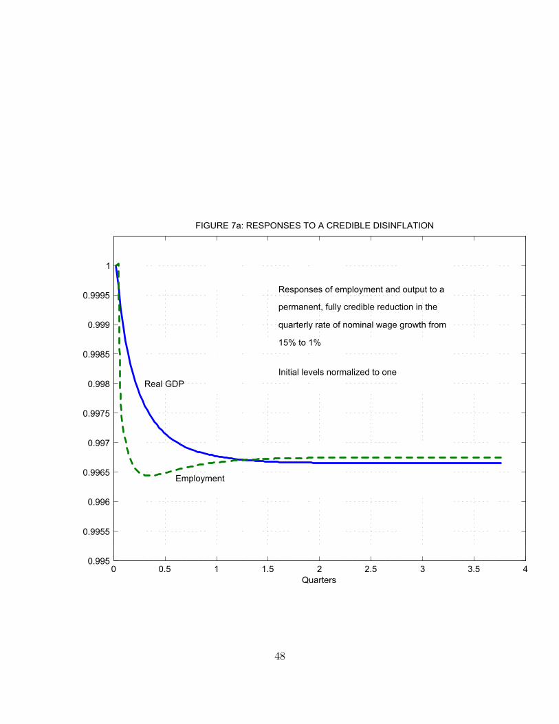
Figure 7a plots the response of two variables–real GDP and employment–

following a one-time permanent and fully credible decrease in the quarterly growth

rate of nominal wages from 15 to 1 percent. Real GDP : is defined simply as the

sum of production of the different goods,

: =Z( )( )

Employment is the equilibrium path of the variable , the labor used to produce

goods and the labor used in re-pricing. Both variables are normalized so that the

initial levels are one. One can see that neither variable declines by as much as one

half of one percent, and this very modest response is completed within a quarter of

the initial shock.

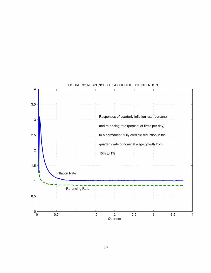
Figure 7b plots the response of the inflation rate and the re-pricing rate to this

same credible disinflation. In constructing the figure, the price level is the fixed-weight

index defined by

: =Z( )( )

and the inflation rate is its quarterly rate of growth. The initial re-pricing rate is

about twice the long-run, post-disinflation level (see Figure 7b) and except for an

initial uptick, the figure shows a small adjustment that is over in less than a month.

The inflation rate follows an erratic path from 15 to 1. The pricing bounds are

narrower with the new, lower rate of wage growth (see Figures 1, 2 and 5) so as soon

25

as the new rate is announced, many firms find themselves with a price level that

is outside the bounds. These firms immediately re-price, some with increases and

others with decreases. These changes almost cancel, and produce the very low initial

inflation rate in the first instant. After that, inflation rises to above 3 percent, and

gradually declines to its new equilibrium level of one. This adjustment, too, is over

in a quarter.

INSERT FIGURES 7a AND 7b

Sargent’s (1986) analysis contrasts the effects of a disinflation that is credible with

the effects of one that is not. There is only one way for a disinflation to be credible,

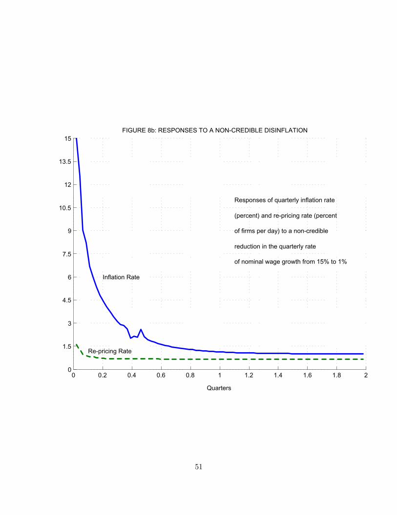
but there are many non-credible ways for it to occur. Figures 8a and 8b represent

one possibility. They describe the results of the following experiment. Consider the

economy in the stationary equilibrium with a constant 15 percent quarterly inflation

rate. Exactly as in the previous example, there is a permanent decrease in the growth

rate of nominal wages from 15 percent to one percent. This decrease is completely

non-credible, in the sense that all the agents in the economy believe that wages will

continue to grow at 15 percent and treat one percent growth as a zero probability

event. Over time they repeatedly observe the one percent growth in but continue

to believe that the next instant the growth rate will revert to its old 15 percent level.

It might be more realistic to assume that agents would use Bayes rule to decide on

the probability of reverting to the high inflationary level, but we will show that

even with our extreme assumption real responses are very small.

The computational strategy for this non-credible case is more complicated than

the one we used to calculate the equilibrium under a credible disinflation, because

beliefs about the consumption aggregator do not coincide with the time path that

actually occurs. Let the original value of the consumption aggregate be (), as in

the credible case, and let the distribution of the firms be the stationary distribution

1(' ) corresponding to Let the inflation rate be 0 for one period. At this point,

26

everyone believes that inflation will revert to immediately and remain there, so that

the original distribution (' ) and the original value of the consumption aggregate

be () will eventually be restored. We assume that this is expected to occur in

9 periods, and define an operator Γ with fixed point exactly as in the perfect

foresight equilibrium described above. This procedure gives everyone’s action in the

first period, corresponding to the actual value 0 and their belief that wage growth

will immediately revert to its original value .

But this belief is not accurate. In the second period, wage growth is 0 again

and everyone believes it will revert to in period 3. But the situation differs from

period 1 because a new distribution 2(' ) 6= 1(' ) has been established. We need

to recalculate a new time path for the consumption aggregate, which will give us

everyone’s behavior in period 2. So we proceed period by period, calculating a perfect

foresight path from each date on, using only the first action to describe what firms

actually do, and discarding the rest of the sequence.

INSERT FIGURES 8a AND 8b

Comparing Figures 8 to the credible disinflation shown in Figures 7, we can see

that as expected, the real effects are larger in the non-credible case: The ultimate

decline in GDP is 0.9 percent rather than 0.3 percent. Even so, the effect is hardly

supportive of the view that the welfare costs of non-credible disinflations are high:

The GDP response remains less than one percent, and the employment response is

only slightly larger. The effects shown on Figures 8 are very persistent, but of course

this is only because we have modeled firms’ beliefs as being unrealistically persistent.

We think the reason for the surprisingly unimportant role played by credibility

in this model is something like the following. Since firms can choose the frequency

of their price changes, they increase it when inflation is high. Each time they adjust

their prices, they expect to adjust them again on average within two months. When

27

disinflation is not credible, the new prices are higher than the ones firms choose

with a credible disinflation, and this reduces output. On the other hand, firms wait

longer than in a credible disinflation to adjust their prices. That means that in the

non-credible disinflation, more firms have prices that are suboptimally low, and they

produce higher outputs. By comparing Figures 7b and 8b, one can see that the re-

pricing rate is lower under non-credible than credible disinflation. These effects work

in opposite directions: The first effect leads to a decline in output while the second

causes it to increase. The resulting overall effect on output is negative but small.8

6. An Impulse-Response Function

In the next section we will describe approximate behavior of the economy in a

two-shock equilibrium, in which firms are subject both to idiosyncratic and aggregate

shocks. It is instructive first, however, to study the dynamics of the model with de-

terministic wage behavior that is subjected to a single, one-time shock to the nominal

wage level. The thought experiment we conduct in this section subjects an economy

in the stationary equilibrium nominal wage rate growth is constant at to an unan-

ticipated jump in the nominal wages from to (1++) , after that the wage growth

resumes its original level

We calculate the response to this shock using the iterative method for calculating

rational expectations equilibrium that we applied to the credible disinflation case in

Section 5. Figures 9a and 9b plot the impulse-response functions calculated in this

way when equals one percent per quarter and + = 0.0125.

INSERT FIGURE 9a AND 9b

First, note that the initial response in output is less than the size of the monetary

8See also Almeida and Bonomo (2002) who use a reduced form menu cost model to analyze effects

of non-credible disinflation.

28

shock. Since aggregate output is

: =Z( )( )

= −1ÃZ µ

¶1−( )

!(1−)(−)×Z µ

¶−( )

the increase of to (1 + +) can increase total output by at most (1 + +)(1−) ×(1 + +) = (1 + +)19

The increase in leads to a temporary increase in the number of the firms

changing their prices. This effect is over very quickly, occuring right after the jump

in wages, after which the frequency of price changes reverts to its steady state level.

The effect on real output lasts longer, but it also declines to zero by the middle of

the first quarter. The reason for such a fast decline is the fact that even if firms do

not react to the aggregate shock alone, many of them re-price due to idiosyncratic

shocks. Once a firm decides to re-price for any reason, it will take the higher level of

nominal wages into account when choosing the new price.

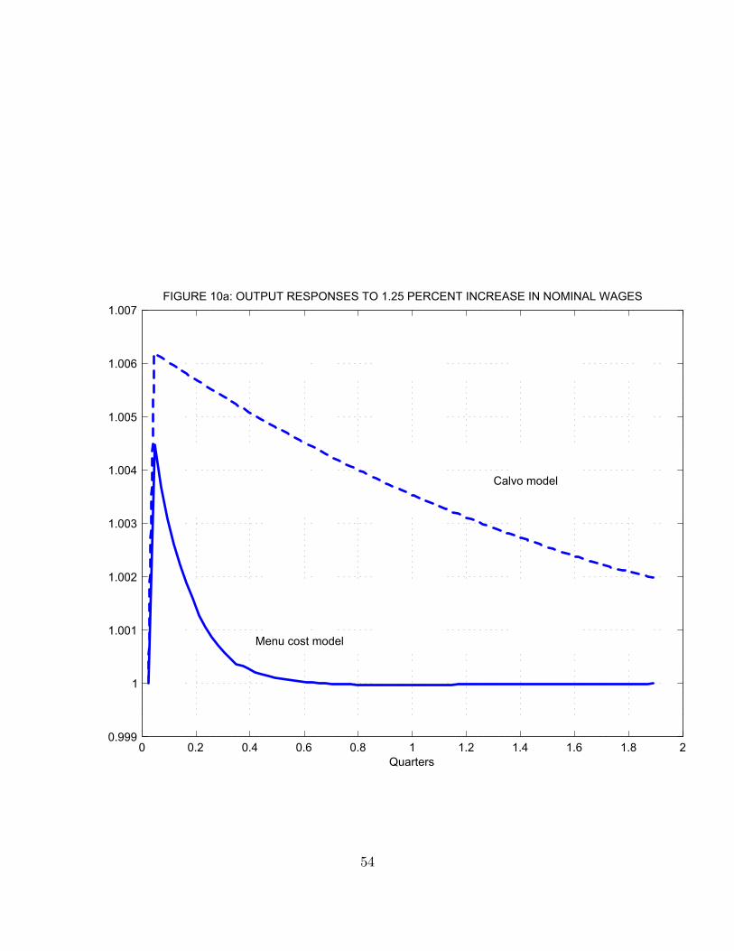
In Figure 10a, we compare the output response to the wage shock described in

Figure 9a to the output response that would occur in a Calvo (1983)-type model,

otherwise identical to ours, in which a firm is permitted to reprice in any period with

a fixed probability that is independent of its own state and the state of the economy.

In the simulation, we set this fixed repricing probability equal to .23 per month, the

frequency predicted by our model. The two curves are strikingly different. The initial

response is much larger with “time-dependent” repricing, as compared to our “state-

dependent” pricing. Time-dependent pricing also implies a much more persistent

effect. These findings underscore the fact that what matters for price rigidity is not

9Also, note that (2.11) and (2.4) imply that =µ

¶1 where is the price aggregate

defined as =£R

1−( )¤1(1−)

This relationship shows that the maximum impact of a

% shock on the consumption aggregate is (1 + )1

29

so much how many prices are changed as it is which prices are changed. The difference

between the two models becomes even larger for bigger shocks. Compare Figure 10b

that shows impulse response to a larger shock to Figure 10a.

INSERT FIGURE 10a AND 10b

These results can be compared with the previous menu cost literature. In the

absence of idiosyncratic shocks, the log-linear approximation of our firms’ problem

would be equivalent to the set-up of Caplin and Spulber (1987). Their result that

aggregate shocks are completely neutral would then hold in ours: In a stationary

equilibrium the distribution of the relative prices of the firms would be uniform, and

a ;% increase in would cause ;% of the firms to adjust their prices. The resulting

distribution of the relative prices would then be the same as the stationary distrib-

ution, and so total output would remain unchanged. The presence of idiosyncratic

shocks introduces more complicated distributions of the relative prices, so in our case

the shock to nominal wages leads to a real responses.

Caplin and Leahy (1991) study a different economy where the level of nominal

wages follow Brownian motion. Their result suggests that response of the output to

the nominal shocks may be very persistent: It is not worth paying the menu cost to

adjust the nominal price if the aggregate shock is small. We show that with reasonably

calibrated idiosyncratic shocks, this effect will be very transient. Even though the

firms do not react to the aggregate shocks per se, they respond to idiosyncratic shocks

and take the higher level of nominal wages into account when they choose a new price.

7. Approximations to a Two-Shock Equilibrium

In Section 2 we defined an equilibrium for an economy subject to two independent

shock process: the nominal wage process (2.1) and the idiosyncratic productivity

process (2.2). All of the results reported in Sections 3-6, though, are based on special

30

cases where the variance 2 of the wage shock is set equal to zero. The only inflation

shocks we have studied are one-time impulses or permanent changes in the drift

parameter.

The only barrier to formulating and studying a Bellman equation for the firm’s

pricing problem in the case where both aggregate and idiosyncratic shocks operate is

the appearance in the firm’s objective function (2.13) of the consumption aggregate

. We have analyzed situations where this aggregate is constant or varies determin-

istically, but if 2 0, is a stochastic process that depends in a complicated way

on the evolution of the distributions of all firms’ prices. In the end of the sectionwe will argue that variations in have a small effect on the aggregate variables for

the calibrated parameter values of the model. We will study an approximate Bellman

equation based on (2.13) but with replaced with an unconditional mean value of

the simulated series for

The Bellman equation suited for this purpose is the variant of (3.5) described in

the Appendix:

)(' ) = max

"Z

0−Π(' ) + − max

0[)('0 ( ))− ]

# (7.1)

where (see (3.6))

Π(' ) = 1−−−[ − −] (7.2)

The processes (' ) are assumed to follow

' = −+ (7.3)

and

= − + (7.4)

The corresponding discrete approximation, analogous to (3.8), is

.(' ) = maxΠ(' )∆+ −∆X00

,('0 0 | ' ).('0 0)

31

max[Π(< )∆+ −∆

X00

,('0 0 | < ).('0 0)]− (7.5)

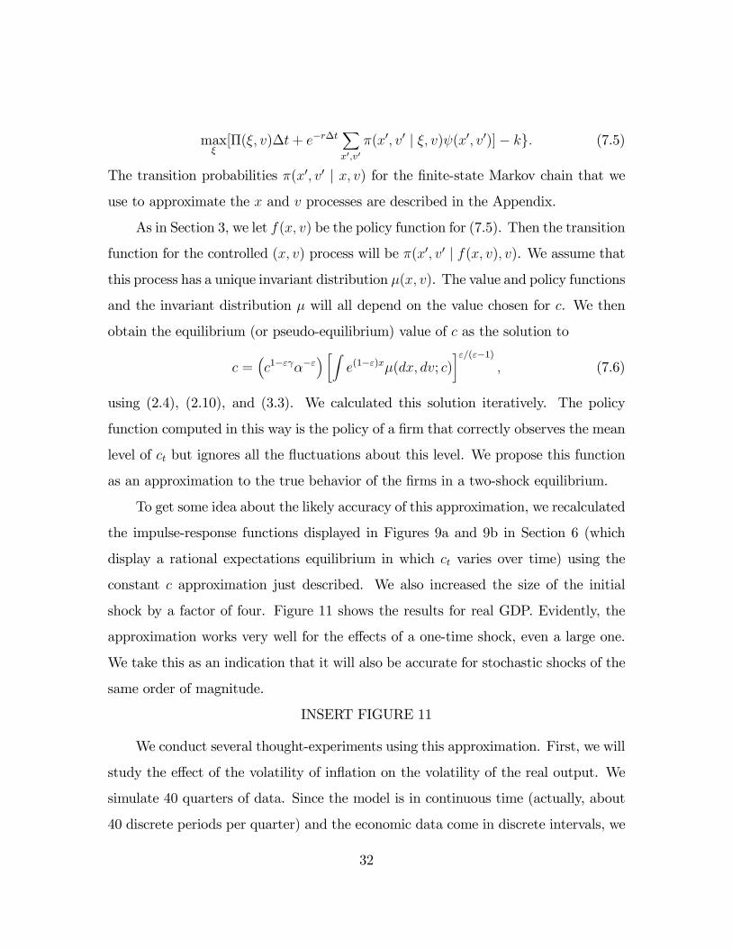
The transition probabilities ,('0 0 | ' ) for the finite-state Markov chain that weuse to approximate the ' and processes are described in the Appendix.

As in Section 3, we let 3(' ) be the policy function for (7.5). Then the transition

function for the controlled (' ) process will be ,('0 0 | 3(' ) ). We assume thatthis process has a unique invariant distribution 4(' ). The value and policy functions

and the invariant distribution 4 will all depend on the value chosen for . We then

obtain the equilibrium (or pseudo-equilibrium) value of as the solution to

=³1−−

´ ·Z(1−)4(' ; )

¸(−1) (7.6)

using (2.4), (2.10), and (3.3). We calculated this solution iteratively. The policy

function computed in this way is the policy of a firm that correctly observes the mean

level of but ignores all the fluctuations about this level. We propose this function

as an approximation to the true behavior of the firms in a two-shock equilibrium.

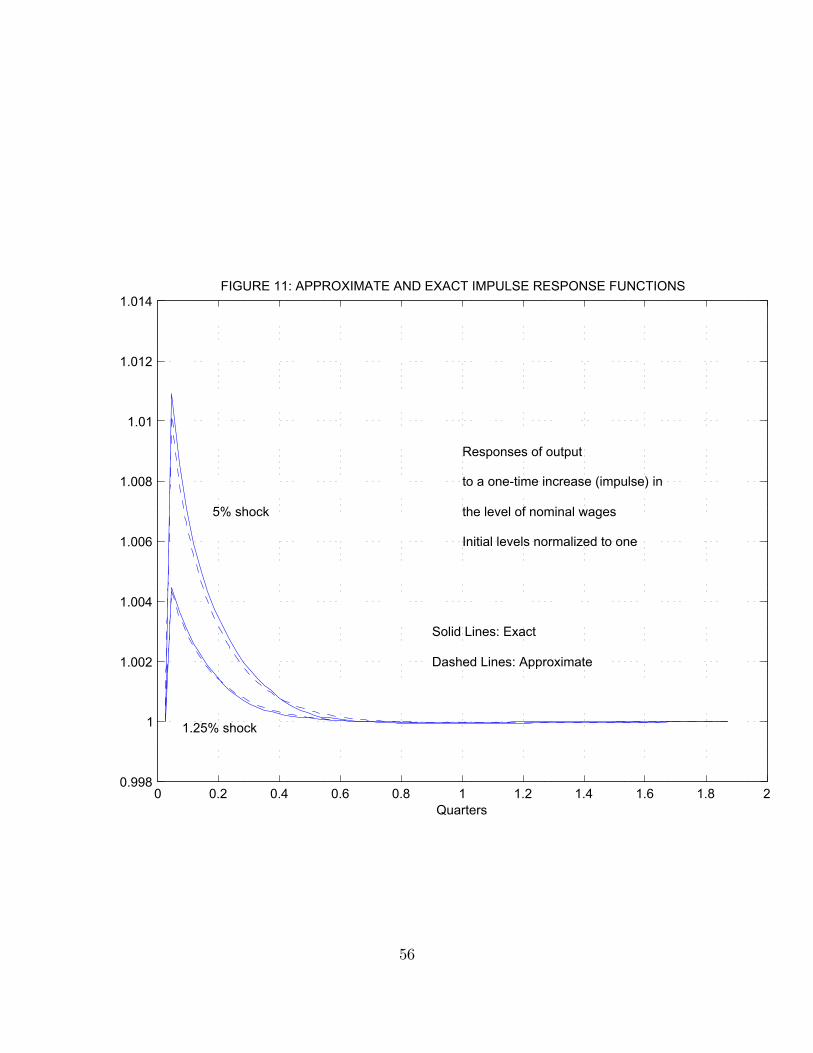
To get some idea about the likely accuracy of this approximation, we recalculated

the impulse-response functions displayed in Figures 9a and 9b in Section 6 (which

display a rational expectations equilibrium in which varies over time) using the

constant approximation just described. We also increased the size of the initial

shock by a factor of four. Figure 11 shows the results for real GDP. Evidently, the

approximation works very well for the effects of a one-time shock, even a large one.

We take this as an indication that it will also be accurate for stochastic shocks of the

same order of magnitude.

INSERT FIGURE 11

We conduct several thought-experiments using this approximation. First, we will

study the effect of the volatility of inflation on the volatility of the real output. We

simulate 40 quarters of data. Since the model is in continuous time (actually, about

40 discrete periods per quarter) and the economic data come in discrete intervals, we

32

aggregate the output of the model into quarterly values by taking the means of the

relevant variables over the quarter. Thus, the level = at quarter of any function

of time =() is defined as

= =Z +1

=()

For our simulations we chose 2 = 00014 which corresponds to the .037 standard

deviation of quarterly inflation in the Klenow and Kryvtsov data set. The standard

deviation of the log level of output is equal to .0017 in our simulation. The stan-

dard deviation of actual U.S. quarterly consumption for the same period (1989 to

1998) around linear trend is equal to .015. Thus monetary fluctuations in this model

can account for only about 10 percent of the observed fluctuations in output. This

estimate is consistent with estimates from other sources.10

In the second experiment we regress the log level of real output on the log dif-

ference of the nominal wages, using the simulated series generated by the model:

ln(: ) = + >[ln( )− ln(

−1)]

In this regression, we obtain the estimate > = 0046 with the standard error 0.007.

Thus an increase in nominal wage rates leads to an increase in real output, as in

standard Phillips curve regressions, but the effect is very small. This conclusion is

not sensitive to different specifications of the parameters ( )

8. Conclusions

We have constructed a model of a monetary economy in which re-pricing of goods

is subject to a menu cost, and studied the behavior of this economy numerically. The

model is distinguished from its many predecessors by the presence of idiosyncratic

shocks in addition to general inflation. We used a data set on individual U.S. prices

10For example, see Lucas’s (2003) survey.

33

recently compiled by Klenow and Kryvtsov to calibrate the menu cost and the variance

and autocorrelation of the idiosyncratic shocks. We conducted several experiments

with the model.

A key prediction of any menu cost model is that the fraction of firms that re-price

in a given time interval will increase with increases in the inflation rate. We simulated

our model at inflation rates varying from zero to 20 percent per quarter. The results,

shown on Figure 6, trace out a curve that passes through the inflation rate-re-pricing

rate pair estimated using data from the low-inflation U.S. economy of the 1990s. The

curve also fits the inflation rate-re-pricing rate pairs observed by Lach and Tsiddon

from the high inflation Israeli economy of 1978-82. We note that a model without

idiosyncratic shocks could not fit both observations.

The model also predicts that credible disinflations will have smaller real effects

that incredible ones: Menu costs make firms reluctant to re-price in response to

transient shocks. We simulated a credible (perfect foresight) reduction in the rate of

wage inflation from 15 percent to one percent, and that re-ran the simulation of a

disinflation that was non-credible in a specified way. The real effects were large in

the second case by a factor of three, but in both simulations this large and sudden

disinflation resulted in output and employment declines of one percent or less.

These results all refer to a special case in which inflation is deterministic. We also

solved an approximation to a more realistic two-shock model. With a realistic inflation

variance, this model can account for perhaps one-tenth of observed variance of U.S.

real consumption about trend. A Phillips curve estimated from data generated by

the model implies that a one percentage point reduction in inflation slope will depress

production by 0.05 of one percent.

In summary, the model we propose fits microeconomic evidence on U.S. pricing

behavior well, and does a remarkably good job of accounting for behavior differ-

ences between countries with very different inflation rates. It does not appear to be

34

consistent with large real effects of monetary instability. These results seem to us

another confirmation of the insight provided by the much simpler example of Caplin

and Spulber (1987) that even when most prices remain unchanged from one day to

the next, nominal shocks can be nearly neutral: The prices that stay fixed are those

where stickiness matters least, and the prices that are far out of line are the ones that

change. Figures 10a and 10b illustrate the quantitative importance of this effect in a

more realistic, calibrated model.

Appendix

The construction of approximating Markov chains for the one shock model of Sec-

tions 3-5 and the two-shock model of Section 6 is based on Kushner and Dupuit

(2001). This appendix provides the details, based on the two-shock model of Section

6. For the most part, the specialization to the one-shock case is obvious.

In the calculations described below, we fix the grid size + and define the state space

= - × as we did in Section 3. Then we approximate the continuous problem

(7.1) with the discrete problem (7.5), repeated as

.(' ) = maxΠ(' )∆+ −∆X00

,('0 0 | ' ).('0 0)

max[Π(< )∆+ −∆

X00

,('0 0 | < ).('0 0)]− (A.1)

where , is a transition function defined on × that we define in a moment. The

time interval ∆ is related to the grid size and other parameters by

∆ =+2

(A.2)

where

= 2 + ++ 2 + + (A.3)

We assume that in a given time interval ∆ at most one of the variables ' and

35

changes.11 Provided that neither ' nor is at its upper or lower bound, we assume

that if ' changes, it moves either to '++ or to '−+; if changes, it moves either to ++ or to −+. The final possibility is that neither of the variables changes and thestate remains at (' ) The probability of all other transitions is zero. Away from

the boundaries of , the five non-zero transition probabilities will then be defined by

,('+ + ' ) =22

(A.4)

,('− + ' ) =22 + +

(A.5)

,(' + + ' ) =22

(if ≥ 0) (A.6)

,(' − + ' ) =22 + +

(if ≥ 0) (A.7)

and

,(' ' ) = 1− 2 + 2 + ++ +

(if ≥ 0) (A.8)

(The () process is symmetric about zero, so the adaptations of (A.6) and (A.7) for

the case ! 0 are obvious.) Transitions at the boundaries are handled by assuming

that if, for example, ' hits its upper bound ' then ' goes one step down to '−+ withprobability ,('−+ ' ) and stays at ' with probability ,('++ ' )+,(' ' )as given by the formulas (A.4) and (A.8). It is evident that the five probabilities (A.4)-

(A.8) add to one, and that the probabilities (A.4)-(A.7) are positive. That (A.8) is

non-negative follows from the fact that | | ≤ .

The first and second moments of the Markov chain we have just defined, condi-

tional on the current state (' ) (assumed not be a boundary point of ) are readily

calculated from (A.4)-(A.8). They are

'(+∆) | '() = ' () = − '

∆= −

11This means that the Markov chains approximating () and () will not be independent for

0, even though the continuous processes are. But independence will hold in the limit, as → 0.

36

(+∆) | ' −

∆= − (if ≥ 0)

?'(+∆) | ' ∆

= 2 + +− ∆

? (+∆) | ' ∆

= 2 + + | |− ( )2∆@ '(+∆) ( +∆) | '

∆= − ∆ (if ≥ 0)

From (A.2) and (A.3)

∆

+=

+

2 + + + 2 + +→ 0 as +→ 0

This is the sense in which the conditional, local moments of the approximating chain

approximate the conditional, local moments of the continuous time ('() ()) process

defined by (7.3) and (7.4). See Kushner and Dupuis (2001), Chapter 9, for a proof

that this approximation converges in distribution to the continuous time diffusion

process when +→ 0.

REFERENCES

[1] Almeida, Heitor, and Marco Bonomo. 2002. “Optimal State-dependent Rules, Cred-

ibility, and Inflation Inertia.” Journal of Monetary Economics, 49: 1317-1336

[2] Basu, Susanto, and John G. Fernald. 1997. “Returns to Scale in U.S. Production:

Estimates and Implications.” Journal of Political Economy, 105: 249-283.

[3] Bils, Mark, and Peter J. Klenow. 2002. ”Some Evidence on the Importance of Sticky

Prices”. NBER Working Paper #9069.

[4] Burstein, Ariel. 2002. “Inflation and Output Dynamics with State Dependent Pricing

Decisions.” Working paper.

37

[5] Calvo, Guillermo A. 1983. “Staggered Prices in a Unitility Maximizing Framework.”

Journal of Monetary Economics, 12: 383-398.

[6] Caplin, Andrew S., and Daniel F. Spulber. 1987. “Menu Costs and the Neutrality of

Money.” Quarterly Journal of Economics, 102: 703-726.

[7] Caplin, Andrew S., and John Leahy. 1991. “State Dependent Pricing and the Dy-

namics of Money and Output.” Quarterly Journal of Economics, 106: 683-708.

[8] Chang, Fwu-Ranq. 1999. “Homogeneity and the Transactions Demand for Money.”

Journal of Money, Credit, and Banking, 31: 720-30

[9] Chari, V.V., Patrick J. Kehoe, and Ellen R. McGrattan. 2000. “Sticky Price Models

of the Business Cycle.” Econometrica, 68: 1151-1180.

[10] Chevalier, Judith A., Anil K. Kashyap, and Peter E. Rossi. 2000. “Why don’t prices

rise during periods of peak demand? Evidence from scanner data.” NBERWork-

ing Paper #7981.

[11] Dixit, Avinash, and Joseph E. Stiglitz. 1977. “Monopolistic Competition and Opti-

mum Product Diversity.” American Economic Review, 67: 297-308.

[12] Dotsey, Michael, Robert G. King, and Alexander L. Wolman. 1999. “State-Dependent

Pricing and the General EquilibriumDynamics of Money and Output.”Quarterly

Journal of Economics, 114: 655-690.

[13] Frenkel, Jacob A., and Boyan Jovanovic. 1980. “On Transactions and Precautionary

Demand for Money.” Quarterly Journal of Economics, 95: 25-43.

[14] Klenow, Peter J. and Oleksiy Kryvtsov. 2003. “State-Dependent or Time-Dependent

Pricing: Does It Matter for Recent U.S. Inflation? Federal Reserve Bank of

Minneapolis working paper.

38

[15] Kreps, David M., and Jose A. Scheinkman. 1983. “Quantity Precommitment and

Bertrand Competition Yield Cournot Outcomes.” The Bell Journal of Eco-

nomics, 14: 326-337.

[16] Kushner, Harold J., and Paul Dupuis. 2001.Numerical Methods for Stochastic Control

Problems In Continuous Time. Second Edition. New York: Springer-Verlag.

[17] Lach, Saul, and Daniel Tsiddon. 1992. “The Behavior of Prices and Inflation: An

Empirical Analysis of Disaggregated Price Data.” Journal of Political Economy,

100: 349-389.

[18] Levy, Daniel, Mark Bergen, Shantanu Dutta, and Robert Venable. 1997. “The Mag-

nitude of Menu Costs: Direct Evidence from Large U.S. Supermarket Chains.”

Quarterly Journal of Economics, 113: 791-825.

[19] Lucas, Robert E., Jr. 2003. “Macroeconomic Priorities.” American Economic Review,

93: 1-14.

[20] Mankiw, N. Gregory. 1985. “Small Menu Costs and Large Business Cycles: A Macro-

economic Model of Monopoly.” Quarterly Journal of Economics, 100: 529-538.

[21] Rotemberg, Julio J., and Michael Woodford. 1995. “Dynamic General Equilibrium

Models with Imperfect Competition.” In Thomas Cooley, ed., Frontiers of Busi-

ness Cycle Research. Princeton: Princeton University Press.

[22] Sargent, Thomas J. 1986. Rational Expectations and Inflation. New York: Harper &

Row.

[23] Sheshinski, Eytan, and Yoram Weiss. 1977. “Inflation and Costs of Price Adjust-

ment.” Review of Economic Studies, 54: 287-303.

39

[24] Sheshinski, Eytan, and Yoram Weiss. 1983. “Optimum Pricing Policy under Stochas-

tic Inflation.” Review of Economic Studies, 60: 513-529.

[25] Spence, Michael E. 1976. “Product Selection, Fixed Costs, and Monopolistic Compe-

tition.” Review of Economic Studies, 43: 217-235.

[26] Stokey, Nancy L. 2002. Brownian Models in Economics. Manuscript.

[27] Willis, Jonathan L. 2000. “General Equilibrium of a Monetary Model with State-

Dependent Pricing.” Working paper.

40

-0.5 -0.4 -0.3 -0.2 -0.1 0 0.1 0.2 0.3 0.4 0.5-0.4

-0.3

-0.2

-0.1

0

0.1

0.2

0.3

0.4

0.5FIGURE 1: PRICING BOUNDS FOR 1% QUARTERLY INFLATION

Log level of productivity v

Rel

ativ

e pr

ice

p-w

Solid lines: upper and lower bounds U(v) and L(v). Dotted line: g(v).

41

-0.5 -0.4 -0.3 -0.2 -0.1 0 0.1 0.2 0.3 0.4 0.5-0.4

-0.3

-0.2

-0.1

0

0.1

0.2

0.3

0.4

0.5FIGURE 2: PRICING BOUNDS FOR 15% QUARTERLY INFLATION

Log level of productivity v

Rel

ativ

e pr

ice

p-w

Solid lines: upper and lower bounds U(v) and L(v). Dotted line: g(v).

42

0 0.5 1 1.5 2 2.5 3 3.5 4 4.5 51.05

1.1

1.15

1.2

1.25

1.3FIGURE 3: SAMPLE PATH OF ACTUAL AND IDEAL PRICE LEVEL k=0.004

Quarters

Pric

e le

vel P

Price without menu costsActual price levelPrice index

43

FIGURE 3A: PRICE OF TRISCUIT 9.5 oz IN

DOMINICK’S FINER FOODS SUPERMARKET IN CHICAGO

Figure 1

Triscuit 9.5 oz

pric

e

week1 399

1.14

2.65

Source: Chevalier, Kashyap and Rossi (2000)

44

0 0.5 1 1.5 2 2.5 3 3.5 4 4.5 51.05

1.1

1.15

1.2

1.25

1.3FIGURE 4: SAMPLE PATH OF ACTUAL AND IDEAL PRICE LEVEL k=0.0004

Quarters

Pric

e le

vel P

Price without menu costsActual price levelPrice index

45

-0.25 -0.2 -0.15 -0.1 -0.05 0 0.05 0.1 0.15 0.2 0.250

0.02

0.04

0.06

0.08

0.1

0.12

0.14

0.16FIGURE 5: DENSITIES OF DEVIATIONS FROM TARGET PRICE

Pricing Error x - x *

1% Quarterly Inflation Rate

(Dashed Line)

15% Quarterly Inflation Rate

(Solid Line)

46

0 2 4 6 8 10 12 14 16 18 20 220

0.05

0.1

0.15

0.2

0.25

0.3

0.35

0.4

0.45

0.5

Quarterly Inflation Rate, Percent

FIGURE 6: FRACTION OF PRICES CHANGED EACH MONTH

Deterministic inflation without firm shock

Deterministic inflation with firm shock

o = (0.9,.22) : Bils-Klenow evidence

x = (15,.41) : Lach-Tsiddon evidence

for 1978-1979

+ = (21,.46) : Lach-Tsiddon evidence

for 1981-1982

47

0 0.5 1 1.5 2 2.5 3 3.5 40.995

0.9955

0.996

0.9965

0.997

0.9975

0.998

0.9985

0.999

0.9995

1

FIGURE 7a: RESPONSES TO A CREDIBLE DISINFLATION

Quarters

Real GDP

Employment

Responses of employment and output to a

permanent, fully credible reduction in the

quarterly rate of nominal wage growth from

15% to 1%

Initial levels normalized to one

48

0 0.5 1 1.5 2 2.5 3 3.5 40

0.5

1

1.5

2

2.5

3

3.5

4FIGURE 7b: RESPONSES TO A CREDIBLE DISINFLATION

Quarters

Inflation Rate

Re-pricing Rate

Responses of quarterly inflation rate (percent)

and re-pricing rate (percent of firms per day)

to a permanent, fully credible reduction in the

quarterly rate of nominal wage growth from

15% to 1%

49

0 0.2 0.4 0.6 0.8 1 1.2 1.4 1.6 1.8 20.986

0.988

0.99

0.992

0.994

0.996

0.998

1

1.002FIGURE 8a: RESPONSES TO A NON-CREDIBLE DISINFLATION

Quarters

Real GDP

Employment

Responses of employment and output

to a non-credible reduction in

the quarterly rate of nominal wage

growth from 15% to 1%

Initial levels normalized to one

50

0 0.2 0.4 0.6 0.8 1 1.2 1.4 1.6 1.8 20

1.5

3

4.5

6

7.5

9

10.5

12

13.5

15FIGURE 8b: RESPONSES TO A NON-CREDIBLE DISINFLATION

Quarters

Inflation Rate

Re-pricing Rate

Responses of quarterly inflation rate

(percent) and re-pricing rate (percent

of firms per day) to a non-credible

reduction in the quarterly rate

of nominal wage growth from 15% to 1%

51

0 0.2 0.4 0.6 0.8 1 1.2 1.4 1.6 1.8 20.999

1

1.001

1.002

1.003

1.004

1.005

1.006

1.007

1.008

1.009FIGURE 9a: RESPONSES TO A TRANSIENT WAGE INCREASE

Quarters

Employment

Real GDP

Responses of employment and output

to a one-time increase (impulse) in

the level of nominal wages of 1.25%

Initial levels normalized to one

52

0 0.2 0.4 0.6 0.8 1 1.2 1.4 1.6 1.8 20

2

4

6

8

10

12

14

16FIGURE 9b: RESPONSES TO A TRANSIENT WAGE INCREASE

Quarters

Inflation Rate

Re-pricing Rate

Responses of quarterly inflation rate

(percent) and re-pricing rate (percent

of firms per day) to a one-time

increase (impulse) in the level of

nominal wages of 1.25%

53

0 0.2 0.4 0.6 0.8 1 1.2 1.4 1.6 1.8 20.999

1

1.001

1.002

1.003

1.004

1.005

1.006

1.007FIGURE 10a: OUTPUT RESPONSES TO 1.25 PERCENT INCREASE IN NOMINAL WAGES

Quarters

Menu cost model

Calvo model

54

0 0.2 0.4 0.6 0.8 1 1.2 1.4 1.6 1.8 20.995

1

1.005

1.01

1.015

1.02

1.025

1.03

1.035FIGURE 10b: OUTPUT RESPONSES TO 5 PERCENT INCREASE IN NOMINAL WAGES

Quarters

Menu cost model

Calvo model

55

0 0.2 0.4 0.6 0.8 1 1.2 1.4 1.6 1.8 20.998

1

1.002

1.004

1.006

1.008

1.01

1.012

1.014FIGURE 11: APPROXIMATE AND EXACT IMPULSE RESPONSE FUNCTIONS

Quarters

Responses of output

to a one-time increase (impulse) in

the level of nominal wages

Initial levels normalized to one

Solid Lines: Exact

Dashed Lines: Approximate

5% shock

1.25% shock

56