NBER WORKING PAPER SERIES

ARE TECHNOLOGY IMPROVEMENTS CONTRACTIONARY?

Susanto BasuJohn Fernald

Miles Kimball

Working Paper 10592http://www.nber.org/papers/w10592

NATIONAL BUREAU OF ECONOMIC RESEARCH1050 Massachusetts Avenue

Cambridge, MA 02138June 2004

We thank Robert Barsky, Menzie Chinn, Russell Cooper, Marty Eichenbaum, Charlie Evans, Jonas Fisher,Christopher Foote, Jordi Galí, Dale Henderson, Michael Kiley, Lutz Kilian, Robert King, Serena Ng,Jonathan Parker, Shinichi Sakata, Matthew Shapiro, Jeffrey Wooldridge, Jonathan Wright and seminarparticipants at a number of institutions and conferences. We also thank several anonymous referees. This isa very substantially revised version of papers previously circulated as Federal Reserve International FinanceDiscussion Paper No. 625 and Harvard Institute of Economic Research Discussion Paper No. 1986. Basu andKimball gratefully acknowledge support from a National Science Foundation grant to the NBER. Basu alsothanks the Alfred P. Sloan Foundation for financial support. We particularly thank Shanthi Ramnath and ChinTe Liu for superb research assistance. This paper represents the views of the authors and does not necessarilyreflect the views of anyone else associated with the Federal Reserve System. The views expressed herein arethose of the author(s) and not necessarily those of the National Bureau of Economic Research.

©2004 by Susanto Basu, John Fernald, and Miles Kimball. All rights reserved. Short sections of text, notto exceed two paragraphs, may be quoted without explicit permission provided that full credit, including ©notice, is given to the source.

Are Technology Improvements Contractionary?Susanto Basu, John Fernald, and Miles KimballNBER Working Paper No. 10592June 2004JEL No. E3, E2, O3, O4

ABSTRACT

Yes. We construct a measure of aggregate technology change, controlling for varying utilization of

capital and labor, non-constant returns and imperfect competition, and aggregation effects. On

impact, when technology improves, input use and non-residential investment fall sharply. Output

changes little. With a lag of several years, inputs and investment return to normal and output rises

strongly. We discuss what models could be consistent with this evidence. For example, standard

one-sector real-business-cycle models are not, since they generally predict that technology

improvements are expansionary, with inputs and (especially) output rising immediately. However,

the evidence is consistent with simple sticky-price models, which predict the results we find: When

technology improves, input use and investment demand generally fall in the short run, and output

itself may also fall.

Susanto BasuDepartment of EconomicsUniversity of Michigan611 Tappan StreetAnn Arbor, MI 48109-1220and NBERsbasu@umich.edu

John FernaldFederal Reserve Bank of Chicago230 South LaSalle StreetChicago, IL 60604-1413jfernald@frbchi.org

Miles KimballDepartment of EconomicsUniversity of Michigan611 Tappan StreetAnn Arbor, MI 48109-1220and NBERmkimball@umich.edu

When technology improves, does employment of capital and labor rise in the short run? Although

standard frictionless real-business-cycle models generally predict that they do, other macroeconomic models

predict the opposite. For example, sticky-price models generally predict that technology improvements cause

employment to fall in the short run, when prices are fixed, but rise in the long run, when prices change.

Sticky-price models also imply that technology improvements could, by reducing short-run investment

demand, cause a short-run decline in output as well as inputs. Hence, correlations among technology, inputs,

investment, and output shed light on the empirical merits of different business-cycle models.

Measuring these correlations requires an appropriate measure of aggregate technology. We construct

such a series by controlling for non-technological effects in aggregate total factor productivity (TFP), i.e., the

aggregate Solow residual: varying utilization of capital and labor, non-constant returns and imperfect

competition, and aggregation effects.1 “Purified” technology varies about half as much as TFP. In addition,

technology fluctuations are countercyclical, in that contemporaneously, they are significantly negatively

correlated with inputs. Contemporaneously, they are uncorrelated with output.

We then explore the dynamic response of the economy to technology. Technology shocks appear

permanent and do not appear serially correlated. Technology improvements reduce hours worked within the

year, but increase hours with a lag of up to two years. Output changes little on impact, but increases strongly

thereafter. Non-residential investment falls sharply on impact before rising above its steady-state level.

Household spending (especially durable consumption and residential investment) rises on impact and rises

further with a lag. Thus, after a year or so, the response to our estimated technology series more or less

matches the predictions of the standard, frictionless RBC model. But the short-run effects do not.

Correcting for unobserved input utilization (labor effort and capital’s workweek) is central for

understanding the relationship between procyclical TFP and countercyclical purified technology. Utilization

is a form of primary input. Our estimates imply that when technology improves, unobserved utilization as

well as observed inputs fall sharply on impact. Both then recover with a lag. In other words, when

technology improves utilization falls—so TFP initially rises less than technology does.

Of course, if technology shocks were the only impulse—and if, as we estimate, these shocks were

negatively correlated with the cycle—then even before controlling for utilization, we would still be likely to

observe a negative correlation between observed TFP and the business cycle. Demand shocks can explain

1 Unless we specifically state otherwise, we use “technology” and “TFP” to refer to growth in these variables. We note that Solow’s (1957) original article suggests modifications and extensions (e.g., for factor utilization and monopoly power) necessary for his residual to properly measure technology at business cycle frequencies; he also notes the issue

2

why, instead, observed TFP is procyclical. When demand increases, output and inputs—including

unobserved utilization—increase as well. We find that shocks other than technology are much more

important at cyclical frequencies, so changes in utilization make observed TFP procyclical.

We identify technology using the tools of Basu and Fernald (1997) and Basu and Kimball (1997), who in

turn build on Solow (1957) and Hall (1990). Basu and Fernald stress the role of sectoral heterogeneity and

aggregation. They argue that for economically plausible reasons—e.g., differences across industries in the

degrees of market power—the marginal product of an input may differ across uses. Growth in the aggregate

Solow residual then depends on which sectors change input use the most over the business cycle. Basu and

Kimball stress the role of variable capital and labor utilization. Their basic insight is that a cost-minimizing firm

operates on all margins simultaneously, both observed and unobserved. Hence, changes in observed inputs can

proxy for unobserved utilization changes. For example, if labor is particularly valuable, firms will tend to work

existing employees both longer (observed hours per worker rise) and harder (unobserved effort rises).

Together, these two papers imply one can construct an index of aggregate technology change by

“purifying” sectoral Solow residuals and then aggregating across sectors. Thus, our fundamental

identification comes from estimating sectoral production functions.

Galí (1999) independently proposes a quite different method to investigate similar issues. Following

Blanchard and Quah (1989), Galí identifies technology shocks using long-run restrictions in a structural

vector autoregression (SVAR); Galí assumes that only technology shocks affect labor productivity in the long

run. He examines aggregate data on output and hours worked for a number of countries and, like us, finds

that technology shocks reduce input use on impact.

A growing literature questions or defends Galí’s (1999) specification.2 Francis and Ramey (2003a)

extend Galí’s identification scheme and subject it to a range of economic and statistical tests; they conclude

that “the original technology-driven real business cycle hypothesis does appear to be dead.” But several

papers critique Galí’s empirical implementation. For example, Christiano, Eichenbaum, and Vigfusson

(2003) and Altig, Christiano, Eichenbaum, and Linde (2002) [henceforth CEV and ACEL] endorse the basic

long-run identification strategy, but argue for using per-capita hours in log-levels rather than in growth rates.

With this subtle change in specification, these two papers conclude that technology improvements raise hours

of aggregation. Basu and Fernald (2001) discuss additional references on technology and TFP. 2 See Galí and Rabanal (2004) for a recent summary.

3

worked on impact.3 Thus, although the SVAR evidence mostly suggests that technology improvements

reduce hours, the evidence from this approach is not yet completely conclusive.

Our alternative augmented-growth-accounting approach yields potentially important evidence that relies

on completely different assumptions for identification. In addition, our approach offers at least three

advantages relative to the SVAR literature. First, our results do not depend on a theoretically derived long-

run identifying restriction that might not hold. For example, increasing returns, permanent sectoral shifts,

capital taxes, and some models of endogenous growth would all imply that non-technology shocks can change

long-run labor productivity; allowing these effects might change the estimated impulse responses.4 Our

production-function approach allows these deviations. Second, even if the long-run restriction holds, it

produces well-identified shocks and reliable inferences only with potentially restrictive, atheoretical auxiliary

assumptions (see, for example, Faust and Leeper, 1997).5 Our production-function approach, by contrast,

does not rely on these same identification conditions. Third, we can look at the effect of technology shocks

on many variables without having to modify our basic identification strategy. In contrast, results from an

identified VAR might look very different as more variables are added.

Nevertheless, the SVAR and augmented-growth-accounting approaches are best regarded as

complements, with distinct identification schemes and strengths. In addition, two additional approaches also

suggest that technology improvements reduce input use. First, estimated structural DGE models (such as

Smets and Wouters, 2003, for the euro area and Galí and Rabanal 2004 for the U.S.) tend to find that

technology improvements reduce input use on impact. Second, Shea (1998) measures technology as

innovations to R&D spending and patent activity and finds that with a lag of several years process

3 However, Fernald (2004) argues that CEV’s specification actually yields stronger results than Galí’s that technology improvements reduce hours worked once one controls for the early 1970s productivity slowdown and mid-1990s re-acceleration in productivity. (This result arises because long run identification schemes can push low frequency correlations into the estimated impact effects.) Thus, correctly interpreted, CEV’s arguments for the levels specification raises our confidence that SVARs imply that technology improvements reduce hours. (CEV and ACEL make several important methodological contributions to the literature, which we view as more substantive than their (fragile) empirical results.) We discuss several related points, including another recent paper by CEV (2004), in Section IV. 4 In the SVAR context, Uhlig (2004) discusses capital taxes and time-varying attitudes towards leisure in the workplace; Sarte (1997) discusses sensitivity to replacing “zero” long-run effect of demand shocks with other reasonable magnitudes (e.g., coming from hysteresis in labor quality). Barlevy (2003) provides a nice model in which cyclical fluctuations have a substantial effect on long-run growth. 5 Cooley and Dwyer (1998) and Erceg, Guerrieri, and Gust (2004) estimate SVARs on data from calibrated DGE models and suggest that these concerns could, in some cases, be important in practice. Nevertheless, Fernald (2004) and

4

innovations increase TFP and simultaneously lower labor input.6

Thus, despite differing data, countries, and methods, the bottom line is that the state-of-the-art versions

of four very different approaches give similar results. It thus appears we have uncovered a robust stylized

fact: technology improvements are contractionary on impact. Given this robustness, we view this as a

stylized fact that models need to explain.

What do these results imply for modeling business cycles? They are clearly inconsistent with standard

parameterizations of frictionless RBC models, including King and Rebelo’s (1999) attempt to “resuscitate”

these models. The negative effect of a technology improvement on non-residential investment is particularly

hard to reconcile with flexible-price RBC models (including the models suggested by Francis and Ramey,

2003a), given our finding that the full impact of a technology improvement on productivity comes almost

immediately. However, our findings are consistent with the predictions of dynamic general-equilibrium

models with sticky prices. Consider the simple case where the quantity theory governs the demand for

money, so output is proportional to real balances. In the short run, if the supply of money is fixed and prices

cannot adjust, then real balances and hence output are also fixed. Now suppose technology improves. Firms

now need less labor and capital to produce this unchanged output, so they lay off workers and desire less

capital, which could reduce investment.7 Over time, however, prices adjust, the underlying real-business-

cycle dynamics take over, and output rises. Relaxing the quantity-theory assumption allows for richer

dynamics for output (which could even decline) and its components, but doesn’t change the basic message.

Of course, in a sticky-price model, technology improvements will be contractionary only if the monetary

authority does not offset their short-run effects through expansionary monetary policy. After all, standard

sticky-price models predict that a technology improvement that increases full-employment output creates a

short-run deflation, which in turn gives the monetary authority room to lower interest rates. In Section V, we

argue that technology improvements are still likely to be contractionary, reflecting the fact that central banks

react with a lag. Indeed, the experience of observing monetary policy in the United States in the 1990s

suggests that central banks observe technology shocks only with a long lag.

Erceg et al do conclude that, when interpreted with suitable caution, SVAR results might be informative. 6 Gali (1998) draws out and discusses this implication of Shea’s findings. 7 Tobin (1955) makes this point in a model with an exogenously fixed nominal wage. Additional issues arise when considering household investment as well as business investment. Investment that adds to capital used in production—with flow benefit equal to a rental rate or marginal product (which depends on the capital/labor ratio and the cost of other inputs)—is distinct from residential investment and consumer durables, for which the rental rate depends largely on income effects and the overall stock of housing and consumer durables.

5

Clearly, our results are not a “test” of sticky-price models of business cycles, even though the results are

consistent with that interpretation. We favor this interpretation in part one wants a model that appropriately

captures the economy’s response to both monetary and technology shocks, and sticky-price models can

generate large monetary non-neutralities. Nevertheless, other explanations are possible, including a flexible-

price world with autocorrelated technology shocks, low capital-labor substitutability, or substantial real

frictions such as habit persistence in consumption and investment adjustment costs; sectoral shifts, if

reallocations are correlated with technology growth; the need to learn about new technologies; and “cleansing

effects” of recessions, in which recessions lead firms to reorganize or, within an industry, eliminate low-

productivity firms. We discuss a range of alternative explanations in Section V.

Some recent direct evidence does suggest that sticky prices are indeed responsible for our finding.

Marchetti and Nucci (2004) apply exactly our identification method to Italian firm-level data and find, like us,

that technology improvements reduce input use. But they also have data on the frequency with which firms

change prices. They find that technology improvements reduce input use only at the firms that have sticky

prices. As well as confirming the negative correlation between technology and hours that we document here,

their finding is strong, direct evidence in favor of our preferred interpretation of this fact.

The paper has the following structure. Section I reviews our method for identifying sectoral and

aggregate technology change. Section II discusses data and econometric method. Section III presents our

main empirical results. Section IV discusses robustness. Section V presents alternative interpretations of our

results, including our preferred sticky-price interpretation. Section VI concludes.

I. Estimating Aggregate Technology, Controlling for Utilization

We identify aggregate technology by estimating (instrumented) industry Hall-style regression equations

with a proxy for utilization. We then define aggregate technology change as an appropriately-weighted sum

of the resulting residuals. Section IA discusses our augmented Solow-Hall approach and aggregation; Section

I.B. discusses how we control for utilization.

A. Firm and Aggregate Technology

We assume each firm has a production function for gross output:

Yi = F i AiKi, Ei Hi Ni ,Mi ,Zi( ). (1.1)

The firm produces gross output, Yi, using the capital stock Ki, employees Ni, and intermediate inputs of energy

and materials Mi. We assume that the capital stock and number of employees are quasi-fixed, so their levels

cannot be changed costlessly. However, firms may vary the intensity with which they use these quasi-fixed

6

inputs: Hi is hours worked per employee; Ei is the effort of each worker; and Ai is the capital utilization rate

(i.e., capital’s workweek). Total labor input, Li, is the product EiHiNi. The firm's production function Fi is

(locally) homogeneous of arbitrary degree γi in total inputs. If γi exceeds one, then the firm has increasing

returns to scale, reflecting overhead costs, decreasing marginal cost, or both. Zi indexes technology.

Following Hall (1990), we assume cost minimization and relate output growth to the growth rate of

inputs. The standard first-order conditions give us the necessary output elasticities, i.e., the weights on

growth of each input.8 Let dx be observed input growth, and du be unobserved growth in utilization. (For

any variable J, we define dj as its logarithmic growth rate ln(

i i

Jt / Jt−1) .) This yields:

( )i i i idy dx du dziγ= + + , (1.2)

where , (1.3) ( )i Ki i Li i i Midx s dk s dn dh s dm= + + + i

i Ki i Lidu s da s dei= + ,

and sJi is the ratio of payments to input J in total cost. Section I.B explores ways to measure dui.

We define “purified” technology change as a weighted sum of industry technology change:

1

iii

Mi

w dzs

−

∑dz = (1.4)

where w equals ( )i PiYi − PMiMi PiYi − PMi Mi( )i∑ ≡ PiV Vi PVV , the firm's share of aggregate nominal value

added. Conceptually, dividing through by 1 Ms− converts gross-output technology shocks to a value-added

basis (desirable because of the national accounts identity that aggregate final expenditure equals aggregate

value added.) These shocks are then weighted by the firm’s share of aggregate value added. Basu and

Fernald (2001, Section III) discuss the interpretation of aggregate technical change as defined in (1.4).9

We define changes in aggregate utilization as the contribution to final output of changes in firm-level

utilization. This, in turn, is a weighted average of firm-level utilization changes:

8 Basu and Fernald (2001) provide detailed derivations and discussion of the equations in this (and the subsequent) subsection. Although we have not noted it explicitly, the detailed derivation allows the firm to potentially charge a markup of price over marginal cost (it must, with increasing returns, to cover its costs). Hence, the resulting estimating equation controls for imperfect competition as well as increasing returns. 9 This weighting scheme follows Domar (1961). In previous work, we defined aggregate technology with (1 )i Misγ− in

the denominator. This definition is convex in iγ . Indeed, as , 1Msγ → [ ]1 (1 )Msγ− → ∞ . This means that positive and negative estimation error does not cancel out; and, indeed, estimation error can have an enormous impact on measured aggregate technology. Domar-weighted residuals are thus more robust to mismeasurement.

7

1

iii

Mi

wdu dus

γ

= − ∑ i

i

(1.5)

From equation (1.2), i duγ enters in a manner parallel to dz , so that (1.6) parallels (1.4). (Note that standard

aggregate TFP (growth), aka the Solow residual, is the special case where all industries have constant returns,

unobserved utilization changes are zero, and factor prices are equal across industries.)

i

Implementing this approach requires disaggregated estimates of returns to scale and variations in

utilization. We observe all other variables necessary to calculate aggregate technology and utilization.

B. Measuring Firm-Level Capacity Utilization

Utilization growth, dui, is a weighted average of growth in capital utilization, Ai, and labor effort, Ei.

Since cost-minimizing firms operate on all margins simultaneously, changes in observed inputs can

potentially proxy for unobserved utilization changes. As in Basu and Kimball (1997), we derive such a

relationship from the firm’s first-order conditions. The model below provides microfoundations for a simple

proxy: Changes in hours-per-worker are proportional to unobserved changes in both labor effort and capital

utilization. We assume only that firms minimize cost and are price-takers in factor markets; we do not require

any assumptions about the firm’s pricing and output behavior in the goods market. In addition, we do not

assume that we observe the firm’s internal shadow prices of capital, labor and output at high frequencies.

We model firms as facing adjustment costs to investment and hiring, so that capital (number of machines

and buildings), K, and employment (number of workers), N, are both quasi-fixed. One needs quasi-fixity for a

meaningful model of variable factor utilization. Higher utilization must raise firms’ costs, or they would always

utilize factors fully. Given these costs, if firms could costlessly change the rate of investment or hiring, they

would always keep utilization at its long-run cost-minimizing level and vary inputs by hiring/firing workers and

capital. Thus, only if it is costly to adjust capital and labor is it sensible to pay the costs of varying utilization.10

We assume that firms can freely vary H, A, and E without adjustment cost. We assume the major cost of

increasing capital utilization, A, is that firms pay a shift premium (a higher wage) to compensate employees for

working at night or other undesirable times. We take A to be a continuous variable for simplicity, although

10 Aggregate models (e.g., Burnside and Eichenbaum, 1996), can model variable utilization without internal adjustment costs, since the representative firm’s input demand affects the real wage and interest rate. But modeling how industries vary utilization in response to idiosyncratic changes in technology or demand requires internal adjustment costs to yield a coherent model of variable factor utilization. (Haavelmo’s (1960) treatment of investment makes these observations.)

8

discrete variations in capital’s workday (the number of shifts) are an important mechanism for varying

utilization.11 When firms increase labor utilization, E, they must compensate workers for the increased disutility

of effort with a higher wage. High-frequency fluctuations in this wage might be unobserved, e.g., if an implicit

contract governs wage payments in a long-term relationship.

An industry’s representative firm minimizes the present value of expected costs:

( ) ( ) ( ) ( ) ( )1

, , , , ,Min 1 ,

s

t j M IA E H M I R s t j t

E r WG H E V A N P M WN D N P K J I∞ −

= =

+ + + Ψ +

∑ ∏ K (1.6)

subject to Y = F AK ,EHN ,M ,Z( ) (1.7)

Kt +1 = It + 1− δ( )Kt (1.8)

1t tN N+ tD= + (1.9)

In each period, the firm’s costs in (1.6) are total payments for labor and materials, and the costs associated with

undertaking gross investment I and hiring (net of separations) D. WG H,E( )V A( ) is total compensation owed per

worker (which, if it takes the form of an implicit contract, may not be observed period-by-period). W is the base

wage; the function G specifies how the hourly wage depends on effort, E, and the length of the workday, H; and

V(A) is the shift premium. PM is the price of materials. WN ( / )NDΨ is the total cost of changing the number

of employees; PIK J I K( ) is the total cost of investment; δ is the rate of depreciation. We assume that Ψ and J

are convex.12 We omit time subscripts.

There are six intra-temporal first-order conditions and two Euler equations, for the state variables K and N.

To conserve space, we analyze only the optimization conditions that affect our derivation; Basu and Kimball

(1997) discuss further details. λ, the multiplier on constraint (1.7), has the interpretation of marginal cost.

denotes derivatives of the production function with respect to argument s, and literal subscripts

denote derivatives of the labor cost function G. We require the first order conditions for A, H, and E:

, 1, 2,3sF s =

11 Beaulieu and Mattey (1998) and Shapiro (1996), for example, apply the variable-shifts model to manufacturing data. 12 We make necessary technical assumptions on G in the spirit of convexity and normality. The conditions on G are easiest to state in terms of the function Φ defined by ln G(H,E) = Φ(ln H, ln E). Convex Φ guarantees a global optimum; assuming Φ11 > Φ12 and Φ22 > Φ12 ensures that optimal H and E move together. We make some normalizations relative to normal or “steady state” levels. Let J δ( )= δ, ′ J δ( )= 1, Ψ 0( ) = 0. We also assume that the

9

A: λF1K = wNG(H, E) ′ V (A) (1.10)

H: λF2 EN = wNGH (H, E)V (A) (1.11)

E: λF2 HN = wNGE (H, E)V (A) (1.12)

Note that uncertainty does not affect our derivations, which rely only on intra-temporal optimization

equations. Uncertainty affects the evolution of the state variables (as the Euler equations would show) but not

the minimization of variable cost at a point in time, conditional on the levels of the state variables.

Equations (1.11) and (1.12) can be combined into an equation implicitly relating E and H:

HGH H, E( )G H ,E( )

=EGE H ,E( )

G H, E( ). (1.13)

The elasticity of labor costs with respect to H and E must be equal because, in terms of benefits, elasticities of

effective labor input with respect to H and E are equal. Given the assumptions on G, (1.13) implies a unique,

upward-sloping E-H expansion path: ( ) ( ),E E H E H′= 0.> That is, we can express unobserved intensity of

labor utilization E as a function of observed hours per worker H. We define ζ ≡ H∗ ′ E H∗( ) E H∗( ) as the

elasticity of effort with respect to hours, evaluated at the steady state. Log-linearizing, we find:

de dhζ= . (1.14)

To find a proxy for capital utilization, we combine (1.10) and (1.11). Rearranging, we find:

1

2

( , ) ( )( , ) ( )H

F AK F G H E AV AF EHN F HG H E V A

′ =

(1.15)

The left-hand side is a ratio of output elasticities. As in Hall (1990), cost minimization implies that they

are proportional to factor cost shares, which we denote by αK and αL . Define g(H) as the elasticity of labor

cost with respect to hours: ( ) ( )( ) ( )( ), ,Hg H H G H E H G E H= H . Define v A as the elasticity of labor

cost with respect to capital’s workweek (equally, the ratio of the marginal to the average shift premium):

( )

( ) ( ) ( )v A AV A V A′= . We can then write equation (1.15) as:

( ) ( ) ( )K Lv A g Hα α= . (1.16)

marginal employment adjustment cost is zero at a constant level of employment: Ψ ′ 0( ) = 0.

10

The function g H is positive and increasing by the assumptions we have made on G H ; let η denote the

(steady-state) elasticity of g with respect to H. The function is positive if the shift premium is positive.

We assume that the shift premium increases rapidly enough with A to make the elasticity increasing in A. Let

( ) ,E( )

( )v A

ω be this elasticity of v. We also assume that αK αL is constant, which requires that F be a generalized

Cobb-Douglas in K and L.13 Under these assumption, the log-linearization of (1.16) is simply

( )da dhη ω= . (1.17)

Thus, equations (1.17) and (1.14) say that the change in hours per worker should be a proxy for changes

in both unobservable labor effort and the unmeasured workweek of capital. The reason that hours per worker

proxies for capital utilization as well as labor effort is that shift premia create a link between capital hours and

labor compensation. The shift premium is most worth paying when the marginal hourly cost of labor is high

relative to its average cost, which is the time when hours per worker are also high.

Putting everything together, we have a simple estimating equation that controls for variable utilization:

.

L Kdy dx s s dh dz

dx dh dz

ηγ γ ζω

γ β

= + + +

= + + (1.18)

We will not need to identify all of the parameters in the coefficient multiplying dh, so we denote that

composite coefficient by β. This specification controls for both labor and capital utilization.14,15

In sum, we estimate equation (1.18) on disaggregated data, which controls for non-constant returns,

imperfect competition, and utilization. We measure industry technology as the residuals dz. We aggregate as

in (1.5) to get a measure of aggregate technology that controls for possible aggregation/reallocation effects.

13 Thus, we assume Y = ZΓ AK( )α K EHN( )α L , M( ), where Γ is a monotonically increasing function. 14 As in Basu and Kimball (1997), allowing capital utilization to affect depreciation would add two more terms. We cannot reject that these terms are zero; in any case, including them has little effect on results reported below. 15 An alternative approach assumes, more restrictively, fixed proportions between an observed and unobserved input. For example, Burnside et al. (1995, 1996) follow Jorgenson and Griliches (1967) and Flux (1913) and suggest that electricity use might proxy for true capital services. This might be reasonable for some manufacturing industries, but it ignores labor effort and is probably more appropriate for heavy equipment than structures.

11

II. Data and Method

A. Data

We seek to measure “true” aggregate technology change, dz, by estimating disaggregated technology

change and then aggregating up to the private non-farm, non-mining U.S. economy. We use industry data

from Dale Jorgenson and collaborators from 1949-1996. The data comprise 29 industries (including 21

manufacturing industries at roughly the two-digit level) that cover the entire non-farm, non-mining private

economy. These sectoral accounts include industry gross output and inputs of capital, labor, energy, and

materials. Appendix I describes the data and our calculations in more detail.

Given the potential correlation between input growth and technology shocks in equation (1.18), we use

instruments uncorrelated with technology change. As described in the data appendix, we use updated

versions of two of the Hall-Ramey instruments: oil prices and growth in real government defense spending.

For oil, we use increases in the U.S. refiner acquisition price. Our third instrument updates Burnside’s (1996)

quarterly Federal Reserve “monetary shocks” from an identified VAR. In all cases, we have quarterly

instruments; we sum the four year t-1 quarterly shocks as instruments for year t.16

B. Estimating Technology Change

We estimate industry-level technology change from the 29 regression residuals from (1.18), estimated as

a system of equations.17 To conserve parameters, we restrict the utilization coefficient within three groups:

durables manufacturing (11 industries, listed in Table 1); non-durables manufacturing (10); and non-

manufacturing (8). Wald and quasi-likelihood ratio tests do not reject these constraints. (Without the

constraints, the variance of estimated technology rises but qualitative and, indeed, quantitative results change

little.) Thus, for the industries within each group, we estimate

i i i i idy c dx dh dziγ β= + + + . (2.1)

This parsimonious equation controls for both capital and labor utilization. Note that hours-per-worker growth

dh essentially enters twice, since it’s also in observed input growth dx. We allow returns-to-scale γi to differ

by industries within a group (hypothesis tests overwhelmingly reject constraints on the γi ). Once estimated,

aggregate ‘purified’ technology change is then the weighted sum of the industry residuals plus constant terms.

Given the mid-sample productivity slowdown, we tested for a break in the industry constants. We

16 The qualitative features of the results in Section III are robust to different combinations and lags of the instruments. Section IV discusses the small sample properties of instrumental variables. 17 Estimation was via GMM in TSP, with NMA=2 (results are not particularly sensitive to this parameter).

12

imposed that any break was common to all industries within each group. Following Andrews (1993), we

considered break dates between the 15th to the 85th percentile of the sample (1955-1988) for six series: TFP

growth for durable manufacturing, non-durable manufacturing, and non-manufacturing; and the

corresponding (aggregated) technology residuals for these groups, estimated without a break. Only in non-

manufacturing do we reject the null of no break.18 In durable manufacturing, technology appears to

accelerate using conventional critical values but not ones (such as Andrews’) that adjust for pre-testing. In

non-durable manufacturing, the technology slowdown is insignificant even at conventional levels.

The data do not speak strongly on whether the non-manufacturing break occurred in 1967 or 1973 and

results are little affected by this choice. Results below impose a 1973 break. Allowing separate trend breaks

for each industry yields results similar to those reported. The breaks are part of the constant terms which we

incorporate into technology. Focusing on residuals alone, however, has little effect on the results we report.

In addition, results are robust to using (unconstrained) industry-by-industry estimation, either by 2SLS

or LIML. Parameter estimates are less precise and more variable with individual than group estimation, but

median estimates are similar to the median GMM estimates. Estimating individual equations raises the

variance of estimated aggregate technology but does not change our main conclusions.

III. Results

A. Estimates and Summary Statistics

Our main focus is the aggregate effects of technology shocks, estimated as an appropriately weighted

average of industry regression residuals. Table 1 summarizes the underlying industry parameter estimates

from equation (2.1). For durable manufacturing, the median returns-to-scale estimate is 1.07; for non-durable

manufacturing, 0.89; for non-manufacturing, 1.10. For all 29 industries shown, the median estimate is 1.00.

(Omitting hours-per-worker growth raises the overall median estimate of returns to scale to 1.12). After

correcting for variable utilization, there is thus little overall evidence of increasing returns, although there is

18 For non-manufacturing TFP, the maximum F statistic was about 16 for a break in 1967 or 1973 (slightly higher 1973). For estimated technology, the maximum F statistic was well above 20 in both 1967 and 1973 (slightly higher 1967). These F statistics exceed the 1-percent critical value of 12.35 from Andrews (1993) for p=1 and π0= 0.15. Boostrapped critical values are similar. For each of durable manufacturing, non-durable manufacturing, and non-manu-facturing, we created 10,000 artificial bootstrapped datasets for both TFP and purified technology. On each artificial dataset, we tested every possible break date (1955 to 1988) and recorded the maximum F statistic. The highest 1-percent critical value across the various productivity or technology series was 13.65 (for non-manufacturing technology).

13

wide variation across industries.19 (Throwing out ‘outlier’ industries (e.g., lumber, textiles, chemicals,

leather, electric utilities, FIRE, and services) has little effect on results below).

The coefficient on hours-per-worker, in the bottom panel, is strongly statistically significant in durables

and non-durables manufacturing. The coefficient is significant at the 10-percent level in non-manufacturing.

Table 2 summarizes means and standard deviations for TFP (the Solow residual) and “purified”

technology. TFP does not adjust for utilization or non-constant returns. Purified technology controls for

utilization and non-constant returns, aggregated as in equation (1.5).

For the entire private non-mining economy, the standard deviation of technology, 1.5 percent per year,

compares with the 2 percent standard deviation of TFP; indeed, the variance is only 55 percent as high. For

both durable and non-durable manufacturing, the standard deviation of purified technology is, perhaps

surprisingly, higher than for TFP. The reduction in variance in column one comes primarily from reducing

the (substantial) positive covariance across industries, consistent with the notion that business cycle factors—

common demand shocks—lead to positively correlated changes in utilization and TFP across industries.

Some simple plots summarize the comovement in our data. Figure 1 plots business-cycle data for the

private economy: growth in TFP, output (aggregate value-added), and hours (all series are demeaned). These

series comove positively, quite strongly so in the case of TFP and output.

Figure 2 plots our purified technology series against these three variables plus estimated aggregate

utilization and non-residential investment. The top panel plots TFP and technology. Technology fluctuates

much less than TFP, consistent with varying input utilization and other non-technological effects raising

TFP’s volatility. Some periods also show a phase shift: TFP lags technology. The second panel plots

aggregate output growth and technology. There is no clear contemporaneous comovement between the two

series. Particularly in the first half of the sample, the series has the same phase shift as does TFP: Output

comoves with technology, lagged one to two years.

The third panel shows one central result: Contemporaneously, hours worked covaries negatively with

technology shocks; the correlation is -0.48. These two series clearly comove negatively over the entire

sample period, although the negative correlation appears more pronounced in the 1950s and 1960s than later.

Following a technology improvement, hours rise with a lag.20 The fourth panel shows that estimated factor

19 Basu and Fernald (2001) discuss the apparent decreasing returns in non-durables manufacturing. 20 Corrections to all three groups—manufacturing durables, manufacturing non-durables, and non-manufacturing—contribute to the negative correlation, although adjustments to manufacturing appear most important. For example, if we simply use TFP in non-manufacturing rather than estimated technology, the correlation with aggregate hours is -0.33.

14

utilization—which, like hours, is a form of input—also covaries negatively with technology. The utilization

pattern explains much of the phase shift in the previous charts. That is, when technology improves, utilization

falls, which in turn reduces measured TFP relative to technology. Utilization generally rises strongly a year

or so after a technology improvement, raising TFP.

The bottom panel (with a much wider scale than the others) shows a second central result: non-

residential investment often falls when technology improves. Conversely, when technology falls (growth

below its mean), investment often rises. (The large investment swings, though, are most likely unrelated to

purified technology.)

As expected, the utilization correction explains most of the reduction in pro-cyclicality. If we simply

subtract estimated utilization growth from TFP, the resulting series has a correlation of -0.3 with hours

growth; various procyclical reallocations then account for the further reduction to a correlation of -0.48.21

B. Dynamic Responses to Technology Improvement

We summarize dynamics with regressions and with impulse responses from small bivariate (near)

VARs. To begin, the level of purified technology appears to have a unit root. With an augmented Dickey-

Fuller test, we cannot reject the null of a unit root (p-value of 0.8) in the level. By contrast, with a KPSS test,

we can reject the null of stationary (with or without a trend); the p-value is less than 0.01. In addition,

technology growth shows little evidence of autocorrelation (e.g., the smallest p-value from the Ljung-Box Q

test is 0.25, when testing for 3rd-order autocorrelation). The point estimates from an autoregression show

slight negative autocorrelation with the second lag and positive correlation at the third lag, but the economic

and statistical effects appear small. Thus, in what follows, we assume technology change is a random walk.

That said, reported results are robust to using autoregressive residuals

Table 3 shows results from regressing a wide range of variables on four lags of technology shocks.

(Since purified technology is close to white noise, using more or fewer lags has little effect on coefficients

shown.)22 Purified technology is a generated regressor, so correct standard errors must account for the

21 As Basu and Fernald (1997) discuss, one reallocation effect comes from the difference in returns to scale between durable and non-durable manufacturing. Durables industries tend to have higher estimated returns to scale (see Table 1) as well as much more cyclical input usage. Hence, during a boom resources are disproportionately allocated to industries where they have a higher marginal product. This generates a procyclical reallocation effect on measured TFP. 22 Conceptually, we interpret our technology shocks as fundamental shocks to a vector-moving-average representation of each series. Assuming these shocks are orthogonal to other fundamental shocks (an assumption that we do not impose for identification), the coefficients are consistent. We report (Newey-West) heteroskedasticity and autocorrelation-robust standard errors. For most variables, minimizing the Akaike or Schwartz Bayesian Information Criteria suggest two lags, at most (this remains true in the VARs, below, which add lags of the variable itself). The regressions show more lags for completeness, since adding them has little impact on the dynamics at zero- to two-lags.

15

estimation error involved in estimating technology from the ‘first step’ parameter estimates in Table 1 and the

underlying industry data. As is typical with generated regressors, the correction depends on the true

coefficient on technology as well as the first-step estimation error (we derive this formally in the appendix).

In particular, if the true coefficient is zero, then the usual standard error calculation is correct. The standard

errors in Table 3 are correct under the null that the true coefficient is zero.

More subtly, however, we want to test the sign of the impact-effect coefficient—e.g., can we reject that

hours rise when technology rises? This hypothesis requires us to reject not only the null hypothesis that the

true coefficient is zero, but that the true coefficient is positive. In principle, with sufficiently large “first-step”

estimation error, it might happen that we could reject that the true coefficient is zero but not reject that the

true coefficient is some positive number. Fortunately, in Appendix II we derive a simple test statistic that

allows us to reject this possibility. Hence, if we can reject the null hypothesis of zero, then we can also reject

the null hypothesis that the true coefficient has the opposite sign from the one reported.

In Table 3, the first row shows that in response to a technology shock, output growth changes little on

impact but rises strongly with a lag of one and two years. Output growth is flat in year three, but below

normal in year four, possibly reflecting a reversal of transient business cycle effects.

The second row summarizes one of the two key points of this paper: When technology improves, total

hours worked fall very sharply on impact. The decline is statistically significant. In the year after the

technology improvement, hours recover sharply. The increase in hours continues into the second year.

Total observed inputs (cost-share-weighted growth in capital and labor), row 3, and utilization, row 4,

show a similar pattern. Note that utilization recovers more quickly but less persistently. In particular, after

the initial decline, utilization rises sharply with a one-year lag but is flat with two lags, even as hours continue

to rise. Economically, this pattern makes sense. The initial response of labor input during a recovery reflects

increased intensity (existing employees work longer and harder). As the recovery continues, however, rising

labor input hours reflects primarily new hiring rather than increased intensity. Thus, one would expect

utilization to peak before total hours worked or employment. Indeed, line 5 shows that employment recovers

more weakly with one lag than does total hours worked. With two lags, however, as utilization levels off,

total hours worked continue to rise because of the increase in employment.

The results for utilization explain the phase-shift in Figure 2. On impact, when technology rises,

utilization falls. Measured TFP depends (in part) on technology plus the change in utilization; the technology

improvement raises TFP, but the fall in utilization reduces it. Hence, on impact TFP rises less than the full

increase in technology. With a one-year lag, utilization increases, which in turn raises TFP.

16

In sum, the estimates imply that on impact, both observed inputs and utilization fall. These declines

about offset the increase in technology, leaving output little changed. With a lag of a year, observed inputs,

utilization, and output, recover strongly. With a lag of two years, observed output and inputs (notably the

number of employees) continue to increase whereas utilization is flat.

The bottom five rows show selected expenditure categories from the national accounts. Line (7) shows

the second key point of this paper: on impact, non-residential investment falls very sharply; with a lag of one

and two years, non-residential investment rises sharply. Thus, the response of investment looks qualitatively

similar to the response of total hours worked.

In contrast, residential investment plus consumer durables purchases rise strongly on impact, then rise

further with a lag. The different response of business and household investment is not surprising. Non-

residential investment is driven by the need for capital in production, whereas the forces driving residential

investment and purchases of consumer durables are more closely connected to the forces driving consumption

generally. Consumption of non-durables and services rises slightly but not significantly on impact and then

rises further (and significantly) with one and two lags. Note that we are largely identifying one time shocks to

the level of technology. Thus, our shocks raise permanent income (though not expected future growth in

permanent income). We therefore expect that consumption should rise in response, although habit formation

or consumption-labor complementarity could explain the initial muted response.

The final two rows show the response of inventories and net exports; in both cases, we deal with the

possibility of negative values by scaling by GDP. The inventory/GDP ratio falls significantly; net

exports/GDP rises, but insignificantly. These are interesting because firms could potentially use these

margins to smooth production, even if they don’t plan to sell more output today. The decline in inventories

could reflect uncertainty about which specific products will be demanded in the future (e.g., if there is

idiosyncratic demand for particular products) so that firms don’t want to smooth production.

Figure 3 plots impulse responses to a 1 percent technology improvement for the quantity variables

discussed above. Although we could simply plot cumulative responses from the regressions in Table 3, we

instead use a complementary approach of estimating bivariate VARs. The impulse responses provide a

simple and parsimonious method of showing dynamic correlations. In particular, we estimate (via seemingly

unrelated regressions) a near-VAR. The first equation involves regressing dz on a constant term; i.e., we

impose that dz is white noise, a restriction consistent with the data. The second equation, for any variable J,

regresses dj on two lags of itself and dz. We derive impulses responses (representing the MA representation)

in the standard way from the estimated equations. Relative to Table 3, the VAR approach conserves degrees

17

of freedom by estimating impulse responses from a parsimonious autoregression. Note that we do not use the

VAR to identify shocks, since we assume that we have already identified exogenous technology shocks.

The impact effect and short-term responses in Figure 3 are generally similar to the regression results. At

longer horizons, the impulse responses suggest that output rises about 1-1/2 times as much as technology;

hours, employment, and total inputs rise a bit (but not significantly) relative to pre-shock levels; utilization

returns close to its pre-shock level; measured TFP rises almost one-for-one with technology; non-residential

investment appears only slightly changed from pre-shock levels but the level of household spending rises.

C. Dynamics of Prices and Interest Rates

Figure 4 shows VAR impulse responses of a range of price and interest rate series. (The regressions

corresponding to Table 3 yield qualitatively similar results). The top row shows deflators for non-farm

business and several economically sensible aggregates: the combination of (residential and non-residential)

investment and consumer durables; and consumption of nondurables and services.23 Focusing on total

nonfarm business, the price level falls about half as much as the technology improvement on impact; prices

continue to fall with one lag and, slightly, with a second lag. The cumulative decline is about 1 percent.

The qualitative results for prices of the two expenditure aggregates are similar. Hence, in the middle

panel, when we look at the relative price of investment (including durables) to consumption (non-durables

and services), we find very little. (The point estimate suggests that the investment deflator rises slightly but

not significantly.) A growing literature focuses on “investment specific” technical change (e.g., Greenwood,

Hercowitz, and Krusell, 1997, and Fisher 2003). Since we use chain-linked data, our technology series, in

principle, incorporates both “neutral” and “investment specific” technology change. That we don’t find a

change in the relative price of investment suggests that technical change, on average, is largely neutral.

The remaining responses on the second row show that the nominal fed funds rate and nominal 3-month

both decline noticeably and remain below normal for an extended period. The third row shows that the real

interest rate appears to decline, but modestly. (Interestingly, the decline is sharper for the fed funds rate than

for the 3-month Treasury rate, reflecting a narrowing of the spread between the two.)

For completeness, we also include real and nominal values of the exchange rate and wage. We use the

23 We use inflation rates, wage growth, and interest rate levels in the VAR along with decadal dummies for the 1970s and 1980s. We plot cumulative effects on price, wage, and interest rate levels.

18

growth rate of the Federal Reserve Board’s broad trade-weighted exchange rate series (this series is available

only since 1973). The exchange rate appears to depreciate very sharply when technology improves. (A word

of caution: the sharp appreciation of 1980-85 and depreciation of 1985-88 dominate the data. Adding

separate dummies for those two periods reduces both the magnitude and statistical significance of the

estimate, which does remain negative.) The nominal wage stays flat; with a fall in the price level, the

measured real wage increases. We hesitate to overinterpret the increase in the real wage, however, since we

are uncertain about the extent to which observed wages are allocative period-by-period.

IV. Robustness checks

We now address robustness. We report a range of VAR specifications and Granger causality tests; put

purified technology into a long-run structural VAR; and look at the industry technology shocks themselves.

Appendices III and IV discuss econometric issues of input measurement error and small-sample-properties of

instrumental variables. Our basic finding that input use covaries negatively with technology survives.

A. Alternative VAR Specifications and Granger Causality

Reported results are affected little if, instead of taking our technology series as white noise, we allow the

series to be autoregressive and/or allow shocks to variable J to affect technology with a lag (e.g., if we use the

standard ordering identification in a VAR). Figure 5 illustrates this robustness with six different estimates of

the hours response and four different estimates of the non-residential investment response. The thick line

with boxes shows the implied response from direct regressions on growth in current and 10 lags of

technology. (This approach uses a lot of degrees of freedom, so the sample period runs from only 1959-1996.

The shorter sample period is the main reason why the direct regression response lies above the other

responses at short horizons.) The thick line with triangles shows our benchmark VAR response, where we

assume that purified technology is an exogenous white-noise process. The two thin lines (almost

indistinguishable in the figures) show results (i) allowing for serial correlation of technology in the VAR, i.e.,

adding lags of technology growth to the technology equation, and (ii) allowing for serial correlation and

(lagged) feedback of shocks to hours on technology (i.e., putting hours growth or investment growth into the

technology equation). In the top panel, the final two dashed lines use BLS nonfarm business hours worked

per capita (aged 16+) rather than Jorgenson’s hours growth, since the SVAR literature focuses on BLS data

(and, indeed, focus on some apparent differences when hours per capita enter in levels or differences). Those

19

specifications allow for serial correlation and feedback. (Results using total BLS private business hours per

capita are similar to the non-farm responses.) It is clear that in these “short-run” specifications, the distinction

between levels and differences is relatively inconsequential.

The bottom line is that the impact effect is very similar in all cases. They uniformly show that hours and

non-residential investment fall on impact and bounce back robustly with one and two lags. The initial

declines are statistically significant in all cases.

This robustness is not surprising, since lags of technology have little explanatory power for current

technology. In addition, the variables we examine in this paper (plus various measures of government

spending) do not appear to Granger-cause technology, so we cannot reject the exogeneity assumption.

CEV (2004) suggest that the level of hours per capita Granger-causes the technology series from an

earlier version of this paper. Neither in levels nor in growth rates are Jorgenson’s or the BLS non-farm

business hours series even remotely significant; e.g., the p-value on two lags of the (log) level of non-farm

business hours per capita (aged 16+) is 0.35. CEV use private business hours rather than non-farm business

hours; the p-value of 0.11 is still insignificant, although it’s much closer.

CEV might perhaps argue that farm hours Granger-causes our technology series,24 but Fernald (2004)

argues that even this relatively high level of significance reflects the productivity slowdown. Both average

technology growth and the level of total business hours per capita were higher before 1973 than after. Indeed,

private business hours per capita appear to Granger-cause the productivity slowdown (using a series that is 1

before 1973 and 0 afterwards): Estimated 1951-96 with two lags, the p-value is 0.02. Since much of the

decline in private business hours reflects movements away from farms, non-farm business hours per capita do

not show the same pattern. Hence, when we estimate the same Granger-causality test with purified

technology that excludes the trend break (and industry constant terms), the p-value for BLS private business

hours rises to 0.39.25 Quite clearly, CEV’s Granger causality evidence reflects a low-frequency correlation,

not high frequency “measurement error” in purified technology.

Nevertheless, our procedure doesn’t require strict exogeneity of technology (so that dzt is independent of

other shocks at time τ, where τ need not equal t). Our identification does require that our instruments not be

24 Hours worked by farmers is poorly estimated relative to the number of employees, which is a reason to prefer non-farm measures. But with two lags, the log of the number of agriculture employees (from the household survey) indeed Granger-causes purified technology with a p-value of under 2 percent. Farm employees proxy nicely for the productivity slowdown, since they fall by more than half from 1949 to 1971 but remain fairly level thereafter. This example points out a limitation of Granger causality tests in this context. 25 With this series, the p-value for whether farm employees Granger-cause purified technology rises to 0.54.

20

correlated contemporaneously with true technology. But suppose, for example, that a positive money

(interest rate) shock leads firms to cut back on R&D, which reduces future technology growth. dzt then

depends on past monetary shocks, which would Granger-cause technology. Nevertheless, it seems likely that

the lags are longer than a year, so that our identification assumption still holds. That said, we find no

evidence that any of the other variables we examine Granger-causes technology.26

B. Long-Run Restrictions

A growing recent literature estimates structural VARs with the long-run identifying restriction that only

technology shocks affect labor productivity in the long run (see, especially, Galí 1999; Francis and Ramey

2003a,b; Christiano, Eichenbaum, and Vigfusson 2003, 2004; and Galí and Rabanal 2004). CEV (2004)

suggest replacing labor productivity with our “purified” technology series; they are concerned that there could

be high frequency cyclical measurement error that the long-run restriction might clean out.27 As in that

literature, we focus on the impulse response of hours to technology, even though (as we discuss below) the

response of business investment to technology may be even more decisive for the key theoretical issues.

Suppose prod is the log of the productivity measure to which one is applies the long-run restriction (e.g.,

labor productivity or the level of purified technology). Suppose hrs is some function of the log of hours

worked; the extant literature mainly focuses on the log-level or the growth rate of hours per capita, but other

specifications use log hours-per-capita detrended in some way or else use the log-level or difference in actual

hours (not per capita). (In larger systems, we can generalize hrs to be a vector of variables that are included

in the VAR, including some function of hours; we don’t consider such systems here). Shapiro and Watson

(1988) show that one can estimate “true” technology residuals as the residuals from the following regression:

1( ) ( )t

Zt tprod c A L prod B L hrst ε−∆ = + ∆ + ∆ +

A(L) and B(L) are polynomials in the lag operator. Note that hrst enters the regression in first differences,

26 In Beaudry and Portier (2000), current behavior reflects (imperfectly) anticipated future changes in technology. Hence, current variables could in principle Granger-cause even completely exogenous future technology. 27 CEV cite “countercyclical markups” which, in our setup, presumably translates into countercyclical returns to scale. However, this effect would not lead to cyclical measurement error. Suppose the true (time-varying) value is tγ but we

estimate a constant γ ; then the estimated error term contains ( )t dxγ γ− . Countercyclical tγ implies that this extra term is always negative, so the main effect is on the constant term rather than the cyclicality of the residual. Note also that Shapiro and Watson’s (1988) argue against using TFP growth, since it is naturally defined in first differences, as is our purified technology dz. In particular, the long-run restriction would label as technology any classical measurement error. Thus, the long-run VAR will not clean out all sources of misspecification.

21

which turns out to be a simple way to impose the restriction that non-technological shocks do not affect the

level of labor productivity in the long run. Since technology shocks might well affect the current growth rate

of hours worked (or other variables included in hrs), we follow Shapiro and Watson and estimate this

regression with instrumental variables (a constant and ∆prodt-s, and the levels of hrst-s+1). 28

Following CEV (2004), we estimate bivariate VARs with two lags, defining prod as ‘purified’

technology. We identify “true” long-run technology shocks as the estimated VAR shock that affects the long-

run level of our purified technology series. We use Jorgenson’s hours series per capita (16+) in both log-

levels and in log-differences. Figure 6 shows the impulse responses from these two specifications. The

responses look qualitatively very similar to the short-run specifications discussed earlier. In particular, both

specifications show strong evidence that technology improvements reduce hours worked; hours then recover

with a lag. (The difference specification is statistically significant at only about the 10 percent level, but the

point estimate is quite similar to the results from short-run identification.)

The resulting technology series has a correlation of 0.82 (levels specification) to 0.97 (difference

specification) with our original purified technology series. Estimating the SVAR with a 1973 trend-break in

productivity brings both correlations to about 0.9. When we define prod as aggregate labor productivity

(following Galí, 1999), including the trend break, the correlation of the resulting technology series with our

purified series is 0.78 (levels) or 0.75 (differences). (Using annual BLS data on non-farm business labor

productivity and hours per capita, the correlations between the identified technology shocks in both the levels

and difference specifications are about 0.6.) Thus, it is clear that we are identifying a similar shock.

Given the sensitivity to low-frequency correlations discussed in Fernald (2004) and Erceg, Gust, and

Guerrieri (2004), one need caution in interpreting results from long-run restrictions. Nevertheless, because

their identification assumptions are very different from ours, they provide useful complementary evidence.

C. One- and Two-Digit Industry Results

Table 5 confirms that results do not arise from aggregation or from a small number of industries. We

correlate industry TFP and purified technology with industry gross output and hours for nine (approximately

28 We estimate impulse responses by putting the estimated technology shock into a second hours equation, in which hrs is regressed on lags of hrs and prod as well as the identified technology shock. The impulse response is then derived via simulation. See CEV (2003) for a clear exposition.

22

one-digit) industries. We also show median correlations for all 29 industries. For all 29 industries, the

median correlation of industry inputs with standard TFP (Corr(dp, dx)) is 0.15; the correlation with purified

technology (dz) falls to -0.33. The median correlation with output falls from 0.57 (TFP) to 0.01

(technology). Technology covaries negatively with inputs in 24 of the 29 industries.

We also correlated industry residuals with SVAR-identified shocks (identified as in Part B, using growth

rates of industry labor productivity and hours). The median correlation of industry SVAR and purified

technology is 0.71; 27 of the 29 correlations are statistically significant at the 95 percent level. For 22

industries, the impact effect of an SVAR-identified technology shock on industry hours is negative.

V. Interpretations of the Results

A. The Standard RBC Model

The data show that technology improvements reduce hours and non-residential investment. By contrast,

the standard RBC model (e.g., Cooley and Prescott 1995) predicts that improved technology should have

raised output, investment, consumption, and labor hours on impact.

Certainly, alternative calibrations of the RBC model could deliver a fall in labor. Technology

improvements raise real wages, which has both income and substitution effects. If the income effect

dominates, labor input might fall.29 But even with strong income effects, it is unlikely that we would observe

the “overshooting” response of hours that we find in the data. The standard RBC model displays monotonic

convergence to the steady state, at least in the linearized dynamics. Thus, if hours fall temporarily due to an

income effect, they should remain low persistently, and converge to their long-run value from below.

Nevertheless, the fall in non-residential investment most strongly contradicts basic RBC theory. In

standard calibrations, a permanent technology improvement increases consumption and investment

together.30 Residential investment and consumer durables display the expected pattern, but business

investment does not. Business investment grows strongly in the second year after technology improves.

Again, this overshooting pattern is not characteristic of standard RBC models.31

29 As in Lindé (2003), positively autocorrelated technology change could also lead workers to take more leisure initially and work harder in the future, when technology is even better; i.e., both income and substitution effects tend to push towards lower current labor supply. However, our technology process is not autocorrelated. 30 In an open economy, especially, one can increase imports, so it is easy to increase both consumption and investment. 31 Our estimates also contradict King and Rebelo’s (1999) attempt to “resuscitate” the RBC model. By adding variable capital utilization to the basic RBC model, they improve the model’s ability to propagate shocks. They use their calibrated model to back out an implied technology series from observed TFP. By construction, their procyclical

23

On the other hand, the effects after two to three years are clearly consistent with RBC models: Output,

investment, consumption, and labor hours are all significantly higher. And the size of the long-run output

response is quantitatively close to the prediction of a balanced growth model: A one percent increase in

Hicks-neutral technology should increase output by 1/(1 )α− percent, where α is the output elasticity of

capital. Assuming constant long-run returns to scale and a capital share of one-third, output should rise by 1.5

percent. The response in Figure 4 (or the cumulated response from Table 3) match this prediction.

Thus, the short-run (but not the medium- and long-run) effects of technology improvements contrast

sharply with the predictions of standard RBC models. However, are those models right in assuming that

technology shocks are the dominant source of short-run volatility of output and inputs? Table 4 reports

variance decompositions from the impulse responses in Figure 3. At the business-cycle frequency of three

years, technology shocks account for more than 40 percent of the variance of output, but only 9 to 17 percent

percent of the variance of different input measures. The patterns are intuitively sensible: hours and utilization

respond much more to technology at high frequencies. (Steady-state growth, of course, requires that long-run

labor supply be independent of the level of technology.) By contrast, technology accounts for only about 18

percent of the initial short-run variance of measured TFP, but 70 percent with a lag of three years. Again, this

pattern accords with our priors: in the short run, changes in utilization and composition account for much of

the volatility of measured TFP. But in the long run, TFP reflects primarily technology.

Our findings thus lie between RBC and New Keynesian positions. Technology shocks are neither the

main cause of cyclical fluctuations, nor negligible. Future models should allow for technology shocks, while

making sure that the impulse responses of a model match those that we and others find.

B. A Flexible-Price Model with “Real Inflexibilities”

Francis and Ramey (2003a) propose a variant of the standard RBC model with inertial consumption and

investment (coming from habit formation and standard q-theory adjustment costs). Hence, domestic demand

changes little when technology improves, so hours worked fall. As Galí and Rabanal (2004) note, this model

is particularly interesting because many business cycle models, with and without nominal rigidities, assume

this kind of real inertia in demand.

The slow rise of non-durables consumption is broadly consistent with the Francis and Ramey (2003a)

technology series, however small, drives business cycles. Our empirical work, by contrast, does not impose such a tightly specified model—and the data reject the King and Rebelo model. Hence, their model is not an empirically relevant explanation of business cycles any more than the basic RBC model is. Instead, the main lesson we take from their paper is the importance of utilization as a propagation mechanism, which applies to more realistic models as well.

24

model, but the response of investment is not. The fall in non-residential investment followed by a large rise a

year later is no more consistent with their model than with the standard RBC model. In general, although the

zero impact effect of technology improvements on output is consistent with their model, the response of

output components is not. Empirically, the lack of an immediate output response incorporates sizable jumps

in two components of investment, in opposite directions. These large jumps are not what one would predict

from a model where investment adjustment costs are highly convex.

C. Price Stickiness

Technology improvements can easily reduce both hours and investment in a sticky-price model.

Suppose the quantity theory governs the demand for money and the supply of money is fixed. If prices

cannot change in the short run, then neither can real balances or output. Now suppose technology improves.

Since the price level is sticky and demand depends on real balances, output does not change in the short run.

But firms need fewer inputs to produce this unchanged output, so they lay off workers, reduce hours and cut

back on fixed investment. (To keep output constant, the sum of the other components of output, such as

consumer durables, residential investment or non-durables and services would have to increase.) Over time,

however, as prices fall, the underlying RBC dynamics take over. Output rises, and the higher marginal

product of capital stimulates capital accumulation. Work hours eventually return to their steady state level.

These effects are present in virtually any dynamic general-equilibrium model with sticky prices, such as

Kimball’s (1998) Neomonetarist model. Kimball (1998) finds that the decline in investment in plant and

equipment induced by a technological improvement can even cause output to decline. Two effects work to

reduce investment. First, as noted above, the demand for all inputs declines, including the demand for capital

services, resulting in a lower rental rate of capital for any given level of output. Second, if a technology

improvement leads to an anticipated decline in the price of investment goods, then firms prefer to hold bonds

instead of investing in plant and equipment on which they will take substantial capital losses. Price declines

follow just this pattern in the data: Figure 4 shows that the price of investment goods falls about 1 percent in

the first two years following a 1 percent technology improvement.

Basu (1998) and Basu and Kimball (2004) calibrate DGE models with staggered price setting, and

reproduce accurately the impact effect of technology improvements that we find in the data.

Of course, the monetary authority is likely to follow a more realistic feedback rule than simply keeping

the nominal money stock constant, as our discussion has assumed. Would it accommodate technology

improvements by loosening policy, thereby avoiding the initial contraction? Basu (1998) allows the monetary

authority to follow a Taylor rule, setting the nominal interest rate in response to lagged inflation and the

25

lagged “output gap”—the deviation between current and full-employment output. He still finds that on

impact, output barely changes when technology improves, while inputs fall sharply. Monetary policy is

insufficiently loose under a Taylor rule in part because the Federal Reserve reacts only with a lag—that is,

after the shock affects inflation or the measured output gap.32

Why do residential investment and consumer durables purchases rise sharply when technology

improves, when investment in plant and equipment falls? On the demand side, business demand for capital

services depends heavily on current levels of other inputs relative to current capital, and this ratio falls after

technology improves; household demand for the services of consumer durables and housing, however,

depends primarily on permanent income, which rises. On the cost side, residential housing purchases appear

to be more sensitive to interest rates than corporate investment. The fed funds rate falls by about a percentage

point in the year that the technology shock occurs (see Figure 4) and the real fed funds rate also declines,

albeit by less. Also, construction prices respond more quickly than the prices of investment goods in general.

Barsky, House, and Kimball (2004) present evidence suggesting that housing prices are relatively flexible,

and they may complete much of their adjustment to the shock within the first year.

The previous discussion suggests that when technology improves, the Fed does indeed respond to the

lower inflation (and perhaps to its perception of the output gap) by lowering the real fed funds rate. Still, it is

certainly possible that the Fed reacts too little. First, it is difficult to recognize in real time that technology

has improved. Even if the Fed perceives that inflation has fallen for one or two quarters, it may not know

whether this fall is a transient blip or is more persistent. Second, estimates of the Fed’s policy rule suggest

the Fed smoothes interest rates (e.g., Clarida, Galí, and Gertler, 1999; Gerlach-Kristen, 2004). Interest rate

smoothing by definition slows down the Fed’s response to shocks.

The best evidence that the Fed does not take sufficient action to offset the contractionary effects of a

technology improvement lies in the behavior of the price level. Since technology shocks change full-

employment output, they do not present the monetary authority with a tradeoff between output and inflation

stabilization.33 Thus, optimal monetary policy would ensure that the technology shock has no effect on

inflation at any horizon, and thus leaves the price level unchanged. But this is not what we observe in the

data: the short-run behavior of prices accords with a model where the Fed does not accommodate technology

32 In Basu’s model, the contraction is relatively short-lived, unlike the responses we find. But Basu’s model incorporates few “real rigidities.” Kimball (1995) shows that one can obtain a “contract multiplier” of any desired size by adding real rigidities to the model, making price adjustment arbitrarily slow. 33 See, e.g,. Woodford, 2003, pp. 461-462, who in turn cites Khan, King and Wolman, 2002, on this point.

26

shocks fully. (In fact, the long-run fall in the price level is almost the same as the long-run increase of output,

indicating a low degree of effective accommodation.)

Galí, López -Salido, and Vallés (2002) suggest that the contractionary effects on inputs is less

pronounced under the Volcker-Greenspan Fed than previously, and advance the hypothesis that monetary

policy was better at accommodating technology improvements in the later period. Table 6 shows regressions

where we allow the coefficients on technology (as well as constant terms) to differ by subsample. We include

current and two lags of technology (we use fewer lags than in Table 3 to conserve degrees of freedom). In the

1949-1979 period, output appears to decline on impact (not significantly), and hours fall sharply and

significantly. In the post-1979 period, output actually rises somewhat on impact; for hours, the point estimate

suggests the impact effect is still negative, but the magnitude is much smaller and the decline is only

marginally significant. The magnitude of the impact decline in non-residential investment is, however, even

larger in the later subperiod. Interestingly, there is virtually no difference in the impact effect on inflation

despite the fact that the fed funds rate falls much more sharply in the post-1979 period. (In the latter period,

the decline in inflation is somewhat less sharp with a lag of one and two years, consistent with the larger and

more persistent decline in the fed funds rate.)

Formal statistical tests for subsample differences, however, do not reject the hypothesis that the

responses of the real variables to technology shocks are the same in the two sub-periods. This is true for both

the impact effect and the cumulative effect of technology. The cumulative effect on the price level, although

not the impact effect, is marginally different at the 10 percent level. Only the response of the Fed Funds rate

is significantly different across the two sub-periods. Hence, our results provide, at best, only weak support

for the hypothesis advanced by Galí, López -Salido, and Vallés (2002).

Finally, as evidence for the role of sticky prices in the short-run effects of technology, Marchetti and

Nucci (2004) apply the basic methods here to a panel of Italian firm-level data. Not only do they confirm our

finding that technology improvements are contractionary, but they find that the observation is driven by the

behavior of firms whose prices are rigid for a year or more. The flexible-price firms do not reduce hours

worked when technology improves. This evidence ties the contractionary result directly to price rigidity.

D. Sectoral Shifts?

Price stickiness can explain why technology improvements are contractionary. Alternatively, even with

flexible prices, if technology change is uneven across sectors, then output and inputs might temporarily fall

because reallocating resources is costly. (Ramey and Shapiro (1998) document these costs for capital.) Our

data, however, do not support the sectoral-shifts alternative.

27

Reallocation pressures presumably depend positively on the dispersion of technology shocks. Thus, we

add a measure of technology dispersion to our basic regressions and see whether it significantly explains input

and output growth.34 . A natural dispersion measure, Disp, is the cross-sectional standard deviation in

technical progress, ( )1 2

2

1

N

it tt ii

Disp w dz dz=

= −

∑

where i indexes industries, dz is the estimated industry

technology shock (scaled to be value-added augmenting), and w is the sector’s value-added weight.

it

i

It seems unlikely that our technology impulse proxies for dispersion effects, since the two variables are

close to uncorrelated. More formally, in Table 7 we regress output growth, various measures of input growth

(total inputs, hours, and utilization), and business investment on purified technology along with current and

two lagged values of Disp (adding more lags makes little or no difference).

In all cases, adding Disp has relatively little effect on the coefficients and standard errors of technology

and its lags. The timing patterns discussed in Section III are unaltered. Most importantly, the addition of the

Disp variables leads to only a moderate improvement in the R2 of the regressions—the increase is between

0.02 and 0.07. (Interestingly, technology dispersion is associated with lower growth in output, utilization,

and business investment with a one year lag; the effect on hours and total inputs appears less significant.)

Overall, the evidence seems more consistent with the sticky-price model of contractionary technology

improvement than with the sectoral-shifts alternative.

E. Time-to-Learn?

Several authors have argued that technological improvements may reduce measured growth for a time,

as the economy adjusts to new production methods.35 For example, Greenwood and Yorukoglu (1997) argue

that the introduction of the PC caused the post-1974 slowdown in economic growth, since workers and firms

had to accumulate new human capital. That is, when new technology is introduced, unobserved investment is

high; but since the national accounts do not include investments in human capital as output, market output—

and hence measured productivity growth—may be relatively low. Therefore, low productivity growth is

associated with high input growth, because “full” output is mismeasured. Over time, the investment in

knowledge does lead to an increase in measured output and productivity.

This class of models does not generally predict our results. We do not correct for mismeasured output

34 Lilien (1982), who argues for the importance of sectoral shifts, measures reallocation as the cross-industry variance of employment growth. Our measure does not rigorously test the sectoral shifts alternative, since a common aggregate shock affects optimal input use equally in all sectors only if all production and demand functions are homothetic. Nevertheless, even if imperfect, our measure should capture some of the forces leading to input reallocation.

28

arising from unobserved investments in knowledge; hence, when technology is introduced, we would

conclude (incorrectly) that technology fell. Since measured (as well as unmeasured) inputs are likely to rise

at those times, we might find that technology contractions coincide with input expansions. But with a lag,

when market output rises, we would measure a technology improvement—coinciding with a boom. Hence,

measured technology improvements would appear expansionary. Figure 2 suggests that the negative

correlation between measured technology and outputs reflects technology improvements as well as declines

(relative to trend), so the learning-time story is unlikely to explain our results.

F. The “Cleansing Effect of Recessions”?

Could causality run from recessions to technical improvement, rather than the reverse? For example, if

recessions drive inefficient firms out of business, then overall productivity might rise.36 This hypothesis

predicts countercyclical productivity, so proponents (e.g., Caballero and Hammour, 1994, p. 1365) have

argued that “other factors (labor hoarding, externalities, etc.) ... make measured productivity procyclical.”

Possibly, by controlling for these “other factors,” we have uncovered the cleansing effects.

With firm-level data, endogenous cleansing would not be a concern. Basu and Fernald’s (1997b)

classify such cleansing effects as “reallocations”—a shift in resources from inefficient to efficient firms—not

a change in firm-level technology. Our theory excludes such effects by adding up changes in firm-level

technology to derive aggregate technology dz. But in practice we use industry data, and estimates of industry

technical change could include intra-industry reallocations. As noted earlier, however, Marchetti and Nucci

(2004) confirm our findings with firm level data. (Of course, there are no firm-level data sets spanning the

economy, so one cannot use firm-level data and address the aggregate macro issues considered here).

In addition, cyclical reallocations are likely to affect estimated returns to scale rather than the cyclicality

of residuals. Suppose that for an industry, dy dx R dzγ= + + , where intra-industry reallocations R depend,

in part, on input growth dx: R = δdx + ξ . A cleansing effect of recessions implies δ <0; ξ captures any

reallocation effects that are uncorrelated with input growth. Even if our instruments are uncorrelated with

technology, they may be correlated with reallocations. Suppose ξ is uncorrelated with either the instruments,

or any cyclical variables. Then ˆplim ( )γ γ δ γ= + < , but the estimated technology shocks do not

incorporate causation from inputs to technology. ξ is a form of classical measurement error in our residuals.

35 See, e.g., Galor and Tsiddon (1997), Greenwood and Yorukoglu (1996), and Basu et al. (2003). 36 This idea goes back at least to Schumpeter. Foster, Krizan, and Haltiwanger (1998) provide empirical evidence on the role of entry and exit in aggregate productivity growth.

29

(This cleansing effect could explain why some of our estimated industry returns to scale are less than one.37)

However, if ξ is correlated with business-cycle variables—reallocations may, for example, depend on

the aggregate cycle as well as sectoral inputs—then some part of our residuals may remain correlated with

output and input changes for reasons of reverse causality.

The cleansing explanation challenges our basic identifying assumption that industry technical change is

exogenous. But Granger causality tests suggest our results are not being driven by reverse causality. That is,

if some of the cleansing effects work with a lag of more than a year, then lagged output or input growth

should predict our measure of technology change. (It is sensible to expect lags, since entry and exit of firms

could be a relatively slow phenomenon.) But we do not find that lagged output or input growth significantly

predicts our measures of technology, providing some evidence against the cleansing interpretation.

A second variant of cleansing models might be termed models of “recessions as reorganizations” (Hall,

1991): Firms might reorganize production when demand is low. This reorganization raises firm-level

technology, so that even firm-level data do not differentiate the sticky-price versus cleansing alternatives. But

this variant of cleansing models generally predicts that when technology improves, investment is also high.

The investment may take the form of job search, as in Hall (1991). But we should also observe higher capital

investment, as Cooper and Haltiwanger (1996) document for the seasonal cycle in the auto industry. Since

non-residential investment falls sharply in the first year following a technology improvement, a flexible-price

reorganization model probably cannot explain the results we find.38

VI. Conclusion

In this paper, we measure aggregate technology by correcting the aggregate Solow residual for

increasing returns, imperfect competition, varying utilization of capital and labor, and aggregation effects.

We reach a robust conclusion: In the short run, technology improvements significantly reduce input use and

non-residential investment; output changes little. Inputs, non-residential investment, and output recover

significantly during the next several years.

These results are inconsistent with standard parameterizations of real-business-cycle models, which

imply that technology improvements raise input use at all horizons. We also find that technology shocks do

37 “Non-cleansing” reallocations can also explain returns to scale (γ) estimates less than one, e.g., if in sub-industries, the cyclicality of input use covaries negatively with returns to scale. This could arise, for example, if high income elasticities (leading to high procyclicality) tend to be associated with high price elasticities of demand (leading to lower steady-state markups, which in turn lead firms to operate at points on their cost curves with lower γ .

30

not account for a very high fraction of the variance of inputs and output at cyclical frequencies. By contrast,

we argue that these results are qualitatively consistent with the predictions of dynamic general-equilibrium

models with sticky output prices driven by both technology and monetary shocks.

Note that our empirical work actually estimates a composite of the partial effect of a technology

improvement and the reactions of policy (especially monetary policy) to that technology shock. If the Fed

tries to stabilize inflation, then the true partial effect is even more contractionary than the total effect that we

estimate. This point may be especially relevant for estimating the dynamic effects of technology shocks—if

the Fed responds in an expansionary way to a fall in inflation and employment, and if some part of Fed policy

operates with a lag of more than one year, it may appear that the economy recovers more quickly from a

technology improvement than would be the case without Fed intervention.

We believe that our paper and the identified-VAR literature have identified an important stylized fact:

Technical progress is contractionary in the short run, but has its expected expansionary effect in the long run.

We advance price stickiness as the major reason for the perverse short-run effect of technical improvement, as

do Galí (1999) and Galí and Rabanal (2004). The evidence is broadly consistent with this view.

Nevertheless, it remains possible that other models could be consistent with the evidence as well. Three of

the competing explanations are “real inflexibilities” in aggregate demand, sectoral-shifts models, and

“cleansing effects” models. We have presented some evidence that these stories do not explain our findings,

but additional, sharper tests are needed before we can be sure that price stickiness does explain our results.

A complication, of course, is that the alternative hypotheses are not mutually exclusive, but could all

contain an element of the truth. Indeed, estimated DGE models by Smets and Wouters (2004) and Galí and

Rabanal (2004) suggest that both nominal and real rigidities play a role.

Nevertheless, if one accepts the view that technology shocks interact with sticky prices, then our results

have important implications for monetary policy. First, monetary policy in the United States over the 1949-

96 time period did not respond sufficiently to technology shocks to allow actual output to adjust quickly to

the new level of full employment output. In this light, the debate in recent years about whether technology

has accelerated—and if so, how monetary policy should react—seems very much on target. Short-run

movements in technology growth matter just as much for the proper conduct of monetary policy as the long-

run rate of technology growth—if not more, since the main concern of monetary policy is short-run

stabilization of the economy around the moving target of full employment output. To the extent that

38 We thank Christopher Foote and Matthew Shapiro for this observation.

31

policymakers can better assess technological movements, monetary policy might be improved in the future.

32

Appendix I: Data and Instruments

We use industry data even though the theory probably applies most naturally to firms. Unfortunately, no firm-level data sets span the economy. Narrowing the focus to a subset of the economy—e.g., using the Longitudinal Research Database—would require sacrificing a macroeconomic perspective, as well as panel length and data quality.

Jorgenson dataset. We use updated data described in Jorgenson, Gollop, and Fraumeni (1987).39 (Barbara Fraumeni, Mun Ho, and Kevin Stiroh were major contributors to various vintages of the data.)

We merged the main dataset, which runs from 1958 to 1996, with an earlier vintage of the datset that runs 1948-1989. We used growth rates from 1949 to 1958 from the older dataset and growth rates 1959 to 1996 from the newer dataset. Growth rates for the post-1959 overlap period generally line up closely, particularly in the early years, so there are not major inconsistencies between the two data series around the merge point. In addition, qualitative results are robust to using the two datasets separately.

We generally construct indices and aggregates as Tornquist indices, with log-changes weighted by average nominal shares in periods t and t-1. However, to construct industry input aggregates, we use factor shares averaged over the entire sample period. We use average factor shares because we are concerned that observed factor payments may not be allocative period-by-period, e.g., because of implicit contracts. This leads us to take an explicit first-order approximation to the industry production function. Results do not appear at all sensitive to this choice, however: Results appear virtually identical using time-varying shares.

We assume that industries earn zero economic profits, so that factor shares sum to one. In U.S. data, pure profits generally appear small (see, e.g., Rotemberg and Woodford 1995). In previous work with older versions of the Jorgenson dataset, we estimated payments to capital as in Hall (1990); estimated profits were generally small, and results were virtually indistinguishable from those that assumed zero profits.

Hours-per-worker. Where available, we used BLS data on hours/worker for production workers. Where necessary, particularly in early years of the sample, we used supplemental employment and hours data provided by Dale Jorgenson and Kevin Stiroh to construct a long time series for each industry. We then detrended hours-per-worker using Christiano-Fitzgerald’s (2003) band pass filter, isolating frequency components between 2 and 8 years. By detrending, our utilization series has zero mean and no trend. We then took the first-difference in this detrended series as our measure of hours-per-worker growth dh. (Detrending log hours/worker with an HP filter or a simple first-difference filter makes little difference to results. In addition, using Jorgenson’s hours/worker data yields very similar results, although the resulting technology series is a bit more volatile.)

National accounts data. All series were downloaded from the Bureau of Economic Analysis, via Haver Analytics database, on April 7, 2004.

Instruments Monetary Shocks. We use quarterly VAR monetary innovations, following Christiano, Eichenbaum, and Evans (1999), Burnside (1996), and others. Following Burnside (1996), we measure monetary policy as innovations to the 3-month Treasury bill rate, since the fed funds market did not exist until the mid-1950s (from 1954:1 through 2003:1, the quarterly average 3-month T-bill rate has a correlation with the fed funds rate of over 0.99). More specifically, we measure monetary shocks as the innovations to the 3-month T-bill rate from a VAR with GDP, the GDP deflator, an index of commodity prices, the 3-month T-bill rate, and M1. (We thank Charles Evans for providing RATS code that estimated the VAR and innovations).40

We sum the quarterly series for the preceding year to obtain an annual series. In principle, we could use

39 Downloaded from http://post.economics.harvard.edu/faculty/ jorgenson/data/35klem.html (Oct 2002). 40 GDP and the GDP deflator are from the BEA via Haver (downloaded May 22, 2003). The 3-month T-bill rate is the rate quoted on the secondary market, from Federal Reserve Board publication H.15 via Haver. M1 is from the Philadelphia Fed real-time dataset. We spliced data from 2003Q1 (from 1959 onwards) to data from 1973Q4 (which covers the pre-1959 period). Charles Evans provided us with the PCOM data used in Christiano, Eichenbaum, and Evans (1999). We extended his PCOM variable back one year, to 1947, by splicing his series with Conference Board data on raw materials spot prices SMP (Haver mnemonic U0M023, downloaded Aug 15, 2003). Following Evans, we filter SMP as follows: . ( ) 1.451 ( 1) 0.586 ( 2) 0.134 ln( ( ))PCOM t PCOM t PCOM t SMP t= ⋅ − − ⋅ − + ⋅ ∆

33

the four quarterly shocks separately as instruments, but the first-stage F-statistic falls sharply. Government Spending. We use the average quarterly growth rate of real government defense spending

from the preceding year, i.e., from the fourth quarter of t-2 to the fourth quarter of t-1, as the instrument for annual input growth from year t-1 to year t.41

Petroleum prices. Following Mork (1989), we base our oil instrument on the “composite” refiner acquisition price (RAP) for crude oil, a series produced by the Department of Energy. The composite price is refiners’ average purchase price of crude oil, i.e., the appropriate weighted average of the domestic and foreign prices per barrel. Conceptually, the major difference between RAP and the PPI for crude petroleum arises from the Nixon price controls imposed in the second half of 1971; controls were not completely removed until the early 1980s and bind particularly sharply in early 1974.42

RAP is available monthly from January 1974 on. However, an annual average series is available from the late 1960s on. We follow Mork (1989) in linking the PPI and the annual composite RAP to create an estimated quarterly refiner acquisition price.43 We assume that before 1974, the refiner price moves one-for-one with the PPI, since the annual growth rate in the composite refiner price moves quite closely with the annual growth in the crude petroleum PPI. In particular, domestic purchases accounted for about 80 percent of refiner purchases and price controls were a minor factor: In 1973, for example, the average RAP for domestic crude oil was $4.17 a barrel while the average RAP for imported oil was $4.08 a barrel. (In 1974, by contrast, the domestic price rose to $7.18/barrel, while the imported price rose to $12.52.)44

We normalize the estimated pre-1974 oil prices so that the average monthly price in 1973 matches the average price in the reported annual composite RAP. Since the PPI is an index, we make a levels-adjustment to get a monthly oil price for the pre-1974 period. The annual composite RAP in 1973 averaged $4.15, so we normalized our derived monthly series to have an average value of $4.15 in 1973. 45

Hamilton (1996) recommends focusing on oil price increases above the peak level over the preceding 12 months. First, Hamilton and others find a nonlinearity: oil price increases are more contractionary than oil price declines are expansionary. Second, he argues that oil price increases have a larger effect if they follow stable prices than if they simply reverse an earlier decline. Thus, we measure the quarterly oil price ‘shock’ as the difference between the log of the quarterly real oil price and the maximum oil price in the preceding four quarters. (In all cases, we measure the quarterly oil price using the last month of the quarter.) For annual data, we take as our instrument the sum of the quarterly shocks in the preceding calendar year.

41 Downloaded from the Bureau of Economic Analysis via Haver Analytics December 12, 2002. 42 Mark French and Rob Vigfusson independently pointed out to us the problems with the PPI. 43 Vigfusson (2002) uses the IMF world spot price of oil. This series, which is not available for our full sample period, moves reasonably closely with the PPI until the first quarter of 1974—when the log change in the IMF world price is 1.37 while the log change in the PPI is 0.32. (IMF Data from International Financial Statistics July 2002 CD-ROM). These changes bracket the price change for U.S. purchasers of oil: In annual data, the 1974 log change in the refiner acquisition price is 0.78; the log-change in the IMF world price is 1.27, compared with 0.52 for the PPI. In sum, we view the composite refiner acquisition price as a better measure of the relative price shock that hit the U.S. economy. 44 From Haver Analytics, we downloaded the PPI for crude petroleum (mnemonic P0561) and the Composite Refiner Acquisition Price for Crude Oil (PZRAC). We downloaded annual RAP data from the Department of Energy at http://www.eia.doe.gov/emeu/aer/txt/ptb0519.html. (All downloads were December 11, 2002) 45 Results appear little affected by alternative ways of linking data over the price-control period 1971 to 1974. For example, we tried a further levels adjustment to exactly match the average price in our constructed series to the actual average 1972 composite price. In addition, we tried deflating by the GDP deflator and also using actual log-change in oil prices rather than using oil price increases only. All of these made little or no perceptible difference to results.

34

Appendix II: The Purified Technology Series as a Generated Regressor46

Our application focuses on hypothesis testing. Arguing that some variable st+j (say current or forwarded employment or investment) covaries negatively with the true technology series ζt(Γ), is equivalent to arguing that the true value of θ in the regression

( )t j t ts α θζ ν+ = + Γ +

is negative. The problem is that θ is estimated from the OLS regression ˆ( ) ,t j t ts vα θζ+ = + Γ +

where is the estimated value of the “first-step” parameters. Testing the null hypothesis that θ is equal to zero would require no generated regressor correction for the asymptotic hypothesis test.

Γ

But arguing that the covariance is negative requires rejecting not only the hypothesis that θ=0, but also rejecting any positive value of θ. Because the test statistic is not monotonic in the true value of θ, rejecting any positive value of θ requires one additional condition beyond rejecting the hypothesis that θ=0. As shown below, the additional condition does not depend on any characteristics of st+j , and so can be interpreted as an overall “quality control” condition on the generated regressor ˆ( )tζ Γ . As long as this overall “quality control” condition on the generated regressor is satisfied, the uncorrected test statistic is valid for asymptotic tests of the hypothesis that 0θ ≥ . The remainder of the appendix demonstrates this claim and spells out the “quality control” condition on the generated regressor.

Our estimation involves a two-step procedure. In the first step, after stacking the industries on top of each other, we can use an instrumental variable row vector qi to estimate the parameter vector Γ in

,t t tdy ξ ε= ΨΓ + where t is time, dyt is a vector of changes in industry log gross output, ξt is a matrix whose “diagonal” elements are the row vectors [1,χ(t>73) ,dxi,dhi] for industry i, Ψ embodies the cross-equation restrictions, and εt is a vector of the demeaned industry-level technology changes, which is the first-step error term. For an appropriately defined rt (see Jeffrey M. Wooldridge 2002, page 140), the estimator satisfies

1/ 2

1

ˆ( ) (1T

t pt

T T r o−

=

Γ − Γ = +∑ ).

We assume that rt is serially uncorrelated. (Since autocorrelation-robust standard errors in the first step are quite similar to uncorrected standard errors, and the estimated aggregate technology shocks themselves are serially uncorrelated, deviations from this assumption are unlikely to be substantial enough to seriously alter the bottom line below.) We can write the usual estimator of the variance-covariance matrix of as Γ

1

1

ˆ ˆ ˆ '.T

t tt

T r r−

=

Φ = ∑

Denote the generated demeaned aggregate technology change by ˆ ˆ( )t tζ ζ= Γ . is a linear combination of the estimated first-step errors

ˆ( )tζ Γ

iε , and so is a function of the data and the estimated value of Γ.

By construction, has a mean of zero. As noted in the main text, we cannot reject the hypothesis that the (demeaned) aggregate technology change is white noise. Imposing the assumption that the true (demeaned) technology change ζ

ˆ( )tζ Γ

t(Γ) is white noise is helpful in delineating the issues that arise because the estimated technology change is a generated regressor. If technology changes are white noise, then the covariance of a current technology change with a given variable conditional on other leads and lags of technology is the same as the unconditional covariance of the current technology change with that variable. The unconditional covariance can be consistently estimated by univariate OLS. The simplicity of univariate OLS greatly clarifies the generated regressor problem in this context.

ˆ( )tζ Γ

As above, let st+j be any variable that is of interest because it might be affected by the technology change

46 We thank Jeff Wooldridge and Serena Ng for helping us with this appendix. All errors remain our own.

35

at time t. For example, st+j could be the current level of aggregate inputs, or a lead of the aggregate input level. In the second step we estimate

ˆ( )t j t ts vα θζ+ = + Γ +

by OLS. Because our focus is on hypothesis testing, we want to know the variance of the estimate θ conditional on a range of values of the true θ. Following Wooldridge (2002, pp 139-141),

ˆ( ) (0,T Normalθ θ− ∼ ),VC+

ˆ ,

where V A with 2ˆ ˆˆplim( 2 ),Bθ θ= −

2 1 2 1 1

1

ˆ ˆ ˆ ˆ ˆ ˆˆˆ{ } 'T

tt

A D T Hr D H H D− − − −

=

= = Φ∑

2 1

1

ˆˆ ˆ ˆˆ ˆ ,T

t t tt

B D T Hrζ ν− −

=

= ∑

2 1 2 2

1

ˆ ˆˆ ˆ ,T

t tt

C D T vζ− −

=

= ∑

1 2

1

ˆˆT

tt

D T ζ−

=

= ∑

and

1

1

ˆˆ ˆ[ ( )T

t tt

H T ζ ζ−Γ

=

],= ∇ Γ∑

where ∇ is the gradient of ˆ( )tζΓ Γ ( )tζ Γ with respect to Γ, evaluated at Γ and expressed as a row

vector. The Cauchy-Schwartz inequality implies that 2ˆ ˆ ˆ 0AC B− ≥

ˆ

. Note that is independent of the particular variable being represented by s

At+j, since v does not appear in its formula. All the extra information

one needs to know from the first-step in order to calculate t

A is Φ , the estimate of the variance-covariance matrix of the first-step parameter vector, together with the gradient vector ˆ(tζ )Γ∇ Γ .

We are interested in showing that θ is negative. (For the most important cases, this is the natural direction. Cases in which we want to show that a covariance of technology shocks with a variable is positive can be handled by defining st+j as the negative of the variable of interest.) Showing that θ is negative can be formalized as a rejection of any hypothesis that has a nonnegative value for θ. That is, for all θ≥0, if κ is the designated critical ratio, we need

2

ˆ( )( ) .ˆ ˆˆ2

TfA B C

θ θθ κθ θ

−= >

− +

If the test statistic f(θ) is monotonically increasing in θ, showing that f(0)>κ is enough to guarantee that f(θ)> κ for all θ>0 as well. However, f(θ) is not, in general, monotonically increasing in θ. Instead, we demonstrate the following Lemma.

Lemma: if then ˆ 0,θ <

min ( ) min( (0), ( )).f f fθ

θ+∈ℜ

≥ +∞

As a consequence, showing that f(0)>κ and that ˆ( ) lim ( ) T

Af f

θθ κ

→+∞+∞ = = >

are together sufficient to guarantee that f(θ)> κ for all θ≥0. Remarks: As noted above, depends only on the details of the first-step estimation and not on the

identity of sA

t+j, so the condition ˆTA

κ> can be seen as an overall “quality control” condition for the

36

generated regressor. (It is often true in applications that no generated regressor correction is needed for rejecting a zero value of a parameter. The complication here is that we need to reject θ>0 as well, which also requires ˆ

TA

κ> .)

For our measure of aggregate technology change, we calculated A , which equals 0.0061. Thus, ˆTA

equals 48 0.0061 = 89 —far in excess of what’s needed to pass this “quality control” condition at any reasonable level of significance.

Proof: The easiest way to demonstrate that min ( ) min( (0), ( ))f f f

θθ

+∈ℜ≥ +∞ as promised is to show that

f(θ) is either (a) monotonically increasing on +ℜ , (b) monotonically decreasing on +ℜ , or (c) first increasing, then decreasing onℜ . The derivative of the test statistic is +

1/ 2 2 3/ 2ˆ ˆ ˆ ˆ ˆˆ ˆ( ) { 2 } [( ) ( )].f T A B C A B C B ˆˆθ θ θ θ θ θ−′ = − + − + −

Thus, the sign of ( )f θ′ is the same as the sign of the linear function ( )ˆ ˆ ˆ ˆˆ ˆ( )A B C Bθ θ θ− + −+ℜ

.

IfC B , then , and f(θ) must be either (a) monotonically increasing on , or (c) first

increasing, then decreasing onℜ , depending on the sign of

ˆ ˆˆ 0θ− ≥ (0) 0≥f ′+ ˆ ˆ ˆA Bθ − . IfC Bˆ ˆˆ 0θ− ≤ , then the Cauchy-

Schwartz inequality implies that 2ˆ ˆ ˆAC B− 0≥ 2 ˆ ˆ ˆ ˆˆ ˆ .B AC ABθ≤ ≤ Since , and dividing both sides by ˆ 0θ < ˆ 0B < B indicates that ˆ ˆˆ ,B Aθ≥

so that Therefore, if , thenˆ ˆ ˆ 0.A Bθ − ≤ ˆ ˆˆ 0C Bθ− ≤ ˆ ˆ ˆ 0A Bθ − ≤ as well, and 1/ 2 2 3/ 2ˆ ˆ ˆ ˆ ˆ ˆˆ ˆ( ) { 2 } [( ) ( )] 0f T A B C A B C Bθ θ θ θ θ θ−′ = − + − + − ˆ ≤

for all θ>0, implying in turn that f(θ) is (b) monotonically decreasing on +ℜ .

Appendix III: Classical Measurement Error in Inputs

Classical measurement error in inputs could, in principle, lead to counter-cyclical measurement error in our technology residuals. However, a simple model suggests that such measurement error cannot explain our results. First, for plausible parameterizations of the importance of measurement error, the “true” correlation remains negative. Second, the observed covariance between measured output and technology, which is zero or negative, bounds the covariance between true technology and true inputs, again suggesting a negative “true” correlation.

In our empirical work, we take the entire regression residual as “technology,” implicitly assuming that our utilization proxies control fully for all variations in utilization. If they do not, but merely provide unbiased estimates of utilization, then the residual includes non-technological “noise” that is completely analogous to classical measurement error. Our model here abstracts from variations in utilization and does not explicitly consider aggregation across industries; neither changes the basic message.

Suppose the true economic model is given by dy dx dzγ∗ ∗= + ∗ , (A.1)

where the starred variables are unobserved, true values. Both output and inputs are measured with error: dy = dy∗ +η (A.2) dx = dx∗ +ε , (A.3)

where η and ε are iid, mean-zero variables with variances and , respectively. Note that the estimated ση2 σε

2

37

variances of dy and dx always exceed their true values: and . σ dx2 = σ dx*

2 +σ ε2 σ dy

2 = σ dy*2 + ση

2

η γε+ −2 2 2 2

*dz η εσ σ σ γ= + +

dz*,dy*)+σ η2

)* * 2,z dx εγσ= −

2

) dz

dz dx dz

εσ σγ

σ σ σ * *

σ = +

σε

σε

cov dz* ,dx*( )

dz*,dy*( )

Now suppose we estimate (A.1) by instrumental variables. If the instruments are uncorrelated with the measurement error, then the estimate of γ is consistent. Hence, in the limit, the only source of error in our estimate of technology change is the measurement error in dy and dx:

dz dz∗= . (A.4) Abstracting from estimation error in γ, equation (A.4) implies that dz σ . Note that for

given observed variance of measured technology, as measurement error becomes larger, the variance of true technology shocks dz*must fall. Using equation (A.4), the covariances of estimated technology change with output and input growth are:

2

cov dz,dy( )= cov( (A.5)

( ) (cov , covdz dx d . (A.6) Measurement error hence biases up both the estimated covariance between output and technology, and

the estimated standard deviation of technology. If the true correlation between output growth and technology change is positive, then the estimated correlation may be biased either towards or away from zero, but cannot turn negative. However, suppose the true correlation between output growth and technology change is negative. Then the estimated correlation is unambiguously towards zero. Thus, our point estimates a negative correlation between output growth and technology change cannot be attributed to measurement error.

However, if the true covariance co is positive, then the estimated correlation is biased down. If the true input covariance is negative, then the estimated correlation might be biased up or down. To assess the the input-mismeasurement bias, we rewrite (A.6) in terms of correlations: Some algebra yields:

* *v( , )dz dx

( *, *) ( , dx

dx

Corr dz dx Corr dz dxσ

By specifying returns to scale and variances, we can calibrate this equation to observed correlations and variances. Suppose returns to scale are constant and that output is measured without error (output measurement error strengthens our case by reducing the variance of true technology), then the maximum σε is 1.41 percent, given that this is the standard deviation of measured technology (since ). In this case, there is no variation in true technology and the true correlation

of inputs and technology is undefined. If instead we assume

2 2 2 2 2* 0dz dz η εσ σ σ γ σ= − − ≥

is 1 percent—still a high number—then *dzσ is also 1 percent. If we define true inputs as the sum of observed utilization plus measured utilization, then observed σ dx is 3.3 percent per year; the “true” correlation between technology and inputs is –0.37, compared with the observed correlation with inputs of –0.50. Even if is 1.35 percent, the true correlation remains at 0.15.

Finally, we are mostly interested in the signs of the correlations rather than their sizes. We can use the upward-biased output covariance to bound the input-covariance from above. Equation (4.1) implies that

cov dz*,dy*( )≥ , (A.7)

(since the variance of dz is positive and ∗ 1γ ≥ ). But we see from equation (4.5) that

cov dz,dy( )≥ cov . Our estimated covariance of output and technology appears to be either approximately zero or even

negative. Thus, we conclude that the true covariance of technology and inputs must also be zero or smaller. Thus, our surprising results about the effects of technology improvements survive considerations of measurement error.

Since we cannot observe measurement error directly, we cannot say how much it affects our results. However, since the bias works against our finding that technology improvements reduce output, it seems likely that technology improvements are in fact contractionary. Furthermore, unlike the simple model used here, our technology change series takes a weighted average of technology shocks across sectors. If measurement error is relatively independent across industries, averaging should attenuate any biases.

38

Appendix IV. Small Sample Properties of Instrumental Variables

Could our results arise from a weak instruments problem? For example, the average F statistic from the

first-stage regression of industry inputs dx on the instruments is 5.4—high enough to be statistically significant. But Staiger and Stock (1997) suggest that instrumental variables estimators sometimes have poor small sample properties when the first-stage F statistic is less than about 10.

Nevertheless, the small sample properties of instrumental variables do not appear to drive our results. First, Staiger and Stock note that LIML has better small sample properties than TSLS. LIML gives results that are qualitatively similar, though with much higher variance, than our preferred results. Second, when we throw out the industries for which the instruments are particularly bad (with first-stage F-statistics for dxi of less than 2), the correlation of technology with hours remains significantly negative.

Third, and more substantively, we pooled industries within groups in order to raise the significance level of the first stage regression; we still find a robust negative correlation of technology and hours. To implement the pooled approach, we stacked industries within groups (durables, non-durables, and non-manufacturing) and then estimated equation (2.1) as a single regression for each group. We thus end up with a separate estimate of γ and β for each group. (In all cases, we removed industry fixed effects by demeaning all variables). The instruments generally appear highly relevant for the stacked regressions, with F statistics for dx that range from 15 to 40; the F statistic for dh ranges from 8 to 28.47 After estimating the pooled regressions, we unstack the residuals into industry residuals, and aggregate as before. The resulting technology series has a correlation of 0.9 with our preferred technology series from Tables 2 and 3. The contemporaneous correlation between technology and hours is a statistically significant -0.39. (It is not surprising that the correlation is a bit less negative than before, given that we lose some of the “reallocation” effects that come from allowing for differences in γ ‘s.)

Finally, we simulated 1000 draws of random, irrelevant instruments and ran our system, deriving 1000 artificial technology series. We then assessed the actual small sample distribution of coefficients and t-statistic from an OLS regression of actual hours growth on estimated technology (contemporaneous only) under the null that the instruments are, in fact, irrelevant. As expected, coefficients are biased towards the OLS estimates—which yield a small positive coefficient, not the negative coefficient we find. In 123/1000 cases, the t-statistic at least as negative as -2; and in 54/1000 cases (5.4 percent), the t-statistic was as negative as (the OLS coefficient) from our main results of -3.6 (this differs slightly from Table 3, since it’s a bivariate regression and it does not calculate Newey-West-corrected standard errors). These frequencies are considerably higher than one would expect from a normal distribution, but it nevertheless suggests it is very unlikely that random instruments explain our results.

Since the pooled specification largely replicates our overall results, we examined what the first-stage F statistics with generated instruments look like. With the pooled data, the median (for all three groups) of the first-stage F statistics with random instruments was 0.9 for dx and 0.8 for dh. Indeed, for none of the 1000 replications were any of the first-stage F statistics for any of the six variables—dx and dh for durable manufacturing, non-durable manufacturing, and non-manufacturing—as large as we actually found in the actual data. Hence, it is exceedingly unlikely that weak instruments alone could explain both our large negative regression coefficient and our relatively high first stage F statistic in the pooled specification.

47 dh in non-manufacturing equal to 8.2 is lower than we would like. But pooled results are virtually unaffected by doing LIML rather than TSLS (since LIML is more robust to small sample issues, though often more variable); and indeed, results are robust to focusing on manufacturing alone.

39

In addition, we looked more closely at the underlying cases where we found a large negative t-statistic.

These generally appear to be cases where one or more of the point estimates of returns to scale are extremely large (e.g., 3 or more). In particular,

• Quantitatively, the negative correlation disproportionately represented the effect of a single industry,48 in contrast to our results;

• The variance of the derived technology shocks tended to be much larger than for our actual purified technology series. (The median ratio of the variances was 2.8, and in only 1 of the cases was the variance smaller with the random instruments.).

In sum, although weak instruments are a concern, they cannot explain our results.

48 Since ( (1i i Miiw dz s= ∑

( , )Vir dz dx Cont= ∑))−

))

dz , the arithmetic contribution CONTi of each sector to the aggregate correlation

(so that Cor ) is Cov . In our reported results, 23 of the 29 industries contribute negatively, with the largest (negative) arithmetic contribution being -0.11 (construction). Of the 123 simulated cases with a negative t-statistic of -2 or larger in magnitude, only 1 simulation had a single contribution as small in magnitude as -0.11. For the cases with a t-statistic at least as large in magnitude as -3, none had a single-industry contribution as small in magnitude as -0.11.

( /(1 ), ) /( ( ) (V Vi i Miw dz s dx stdev dz stdev dx− i

40

References Altig, David, Lawrence Christiano, Martin Eichenbaum, and Jesper Lindé (2003). “Technology Shocks and

Aggregate Fluctuations.” Manuscript. Andrews, Donald (1993). "Tests for Parameter Instability and Structural Change with Unknown Change

Point," Econometrica, 61, 821–856. Barlevy, Gadi (2003). “The Cost of Business Cycles under Endogenous Growth.” Manuscript. Basu, Susanto (1996). “Cyclical Productivity: Increasing Returns or Cyclical Utilization?” Quarterly

Journal of Economics 111 (August): 719-751. ______ (1998). “Technology and Business Cycles: How Well Do Standard Models Explain the Facts?”

Beyond Shocks: What Causes Business Cycles? Federal Reserve Bank of Boston: Boston. Basu, Susanto and John Fernald (1997). “Returns to Scale in U.S. Production: Estimates and Implications.”

Journal of Political Economy 105 (April) 249-283. ______ (2001). “Why Is Productivity Procyclical? Why Do We Care?” New Directions in Productivity

Analysis, edited by Edwin Dean, Michael Harper and Charles Hulten. (Studies in Income and Wealth Volume 63). University of Chicago Press, 2001.

______ (2002). “Aggregate Productivity and Aggregate Technology.” European Economic Review, June. Basu, Susanto and Miles Kimball (1997). “Cyclical Productivity with Unobserved Input Variation.” NBER

Working Paper 5915. ______ (2004). “Investment Planning Costs and the Effects of Fiscal and Monetary Policy,” unpublished,

University of Michigan.

Beaudry, Paul and Franck Portier (2000). “An Exploration into Pigou’s Theory of Cycles.” Manuscript, University of British Columbia.

Beaulieu, John J. and Joseph Mattey (1998). “The Workweek of Capital and Capital Utilization in

Manufacturing.” Journal of Productivity Analysis. 10 (October): 199-223. Bils, Mark and Jang-Ok Cho (1994). "Cyclical Factor Utilization." Journal of Monetary Economics 33, 319-

354. Blanchard, Olivier and Daniel Quah (1989). “The Dynamic Effects of Aggregate Demand and Supply

Disturbances.” American Economic Review 79 (4): 654-673. Burnside, Craig (1996). “What do Production Function Regressions Tell Us about Increasing Returns to

Scale and Externalities?” Journal of Monetary Economics 37 (April): 177-201. Burnside, Craig, Martin Eichenbaum, and Sergio Rebelo (1995). “Capital Utilization and Returns to Scale.”

In B. Bernanke and J. Rotemberg, eds., NBER Macroeconomics Annual 1995 (MIT Press). ______ (1996). “Sectoral Solow Residuals.” European Economic Review 40:861-869. Caballero, Ricardo J. and Mohamad L. Hammour (1994). “The Cleansing Effect of Recessions.” American

Economic Review 84(December): 1350-68. Christiano, Lawrence J., Martin Eichenbaum, and Charles Evans (1999). “Monetary Policy Shocks: What

41

Have We Learned and to What End?” Handbook of macroeconomics. Volume 1A, pp. 65-148, Handbooks in Economics, vol. 15. New York: Elsevier Science, North-Holland,

Christiano, Lawrence, Martin Eichenbaum, and Robert Vigfusson (2003). “What Happens After a

Technology Shock?” NBER Working Paper No. 9819.

______ (2004). “The Response of Hours to a Technology Shock: Evidence Based on a Direct Measure of Technology.” NBER Working Paper No. 10254.

Christiano, Lawrence J. and Terry J. Fitzgerald (2003). “The Band Pass Filter.” International Economic Review, May 2003, v. 44, iss. 2, pp. 435-65.

Cooley, Thomas F and Mark Dwyer (1998). “Business Cycle Analysis without Much Theory: A Look at

Structural VARs.” Journal of Econometrics 83: 57-88. Cooley, Thomas F. and Edward C. Prescott (1995). “Economic Growth and Business Cycles.” In Thomas F.

Cooley, ed., Frontiers of Business Cycle Research. Princeton: Princeton University Press. Cooper, Russell and John Haltiwanger (1996). “Evidence on Macroeconomic Complementarities.” Review

of Economics and Statistics 78 (February): 78-93. Domar, Evsey D. (1961). “On the Measurement of Technical Change.” Economic Journal 71: 710-729. Erceg, Christopher J., Guerrieri, Luca and Gust, Christopher J., "Can Long-Run Restrictions Identify

Technology Shocks?" (January 2004). FRB International Finance Discussion Paper No. 792.

Faust, Jon and Eric M. Leeper (1997). “When Do Long-Run Identifying Restrictions Give Reliable Results?” Journal of Business and Economic Statistics (July): 345-53.

Fernald, John (2004). “Trend Breaks, Long Run Restrictions, and the Contractionary Effects of Technology

Shocks.” Manuscript, Federal Reserve Bank of Chicago. Fisher, Jonas (2003). “Technology Shocks Matter.” Manuscript, Federal Reserve Bank of Chicago. Flux, A. W. (1913). “Gleanings from the Census of Productions Report.” Journal of the Royal Statistical

Society 76(6): 557-85. Foster, Lucia, C.J. Krizan, and John Haltiwanger (1998). “Aggregate Productivity Growth: Lessons from

Microeconomic Evidence.” NBER Working Paper No. 6803. Francis, Neville and Valerie Ramey (2003a). “Is the technology-driven real business cycle model dead?

Shocks and aggregate fluctuations revisited.” Manuscript. Francis, Neville and Valerie Ramey (2003b). “The Source of Historical Economic Fluctuations: An

Analysis Using Long-Run Restrictions.” Manuscript. Fuhrer, Jeffrey C. and George R. Moore (1995). “Inflation Persistence.” Quarterly Journal of Economics

110 (February): 127-159. Galí, Jordi (1998). “Comment.” In Ben S. Bernanke and Julio J. Rotemberg, eds., NBER Macroeconomics

Annual 1998. MIT Press: Cambridge, MA. ______ (1999). “Technology, Employment, and the Business Cycle: Do Technology Shocks Explain

Aggregate Fluctuations?” American Economic Review, 89 (March): 249-271. Galí, Jordi and Pau Rabanal (2004). “Technology Shocks and Aggregate Fluctuations: How Well Does the

42

RBC Model Fit Postwar U.S. Data?” Paper presented at NBER Macroeconomics Annual conference. Galí, Jordi, J. David López -Salido, and Javier Vallés (2002). “Technology Shocks and Monetary Policy:

Assessing the Fed’s Performance,” Journal of Monetary Economics, vol. 50, 2003, 723-743. Galor, Oded and Daniel Tsiddon (1997). “Technological Progress, Mobility, and Economic Growth.”

American Economic Review 87 (June): 363-82. Gerlach-Kristen, Petra, 2004. "Interest Rate Smoothing: Monetary Policy Inertia or Unobserved Variables?"

Contributions to Macroeconomics, Vol. 4 (1), article 3, Berkeley Electronic Press. Greenwood, Jeremy and Mehmet Yorukoglu (1997). “1974.” Carnegie-Rochester Conference Series on

Public Policy, June, 46: 49-95. Greenwood, Jeremy & Hercowitz, Zvi & Krusell, Per, 1997. "Long-Run Implications of Investment-Specific

Technological Change," American Economic Review, Vol. 87 (3) pp. 342-62. Hall, Robert E. (1990). “Invariance Properties of Solow's Productivity Residual.” In Peter Diamond (ed.)

Growth,Productivity, Unemployment (Cambridge, MA: MIT Press). ______ (1991). “Labor Supply, Labor Demand, and Employment Volatility,” in Olivier J. Blanchard and

Stanley Fischer, eds., NBER Macro Annual. Hamilton, James D. (1996). “This Is What Happened to the Oil Price-Macroeconomy Relationship.” Journal

of Monetary Economics, v. 38, iss. 2 (October), pp. 215-20 Jorgenson, Dale W. and Zvi Griliches (1967). “The Explanation of Productivity Change.” Review of

Economic Studies 34: 249-283. Jorgenson, Dale W.; Gollop, Frank and Fraumeni, Barbara (1987). Productivity and U.S. Economic Growth.

Cambridge: Harvard University Press. Kahn, Aubhik, Robert G. King, and Alexander L. Wolman (2002)., “Optimal Monetary Policy,” NBER

Working Paper # 9402. Kimball, Miles S. (1995). “The Quantitative Analytics of the Basic Neomonetarist Model.” Journal of

Money, Credit, and Banking 27 (November): 1241-77. ______ (1998). “The Neomonetarist KE-LM Model.” Manuscript, University of Michigan. ______ (2003). “Q-Theory and Real Business Cycle Analytics.” Manuscript, University of Michigan. King, Robert G. and Sergio Rebelo (1999). “Resuscitating Real Business Cycles.” Handbook of

Macroeconomics. Volume 1B. North-Holland: Amsterdam. pp. 927-1007 Lilien, David M. (1982). “Sectoral Shifts and Cyclical Unemployment.” Journal of Political Economy 90

(August) 777-793. Lindé, Jesper (2003) “The Effects of Permanent Technology Shocks on Labor Productivity and Hours in the

RBC-Model.” Manuscript. Marchetti, Domenico and Francesco Nucci (2003). “Price Stickiness and the Contractionary Effect of

Technology Shocks.” European Economic Review. Mork, Knut Anton (1989). “Oil and the Macroeconomy When Prices Go Up and Down: An Extension of

43

Hamilton's Results.” Journal of Political Economy, v. 97, iss. 3 (June), pp. 740-44 Ramey, Valerie A. and Shapiro, Matthew D. (1998). “Costly Capital Reallocation and the Effects of

Government Spending.” Carnegie-Rochester Conference Series on Public Policy, 48 (June): 145-94. Sarte, Pierre-Daniel (1997). “On the Identification of Structural Vector Autoregressions.” Federal Reserve

Bank of Richmond Economic Quarterly 83 (Summer): 45-67. Shapiro, Matthew D. (1996). “Macroeconomic Implications of Variation in the Workweek of Capital.”

Brookings Papers on Economic Activity (2): 79-119. Shapiro, Matthew D. and Mark Watson (1988). “Sources of Business Cycle Fluctuations,” in Stanley Fischer

ed, NBER Macroeconomics Annual 1988. Shea, John (1998). “What Do Technology Shocks Do?” In Ben S. Bernanke and Julio J. Rotemberg, eds.,

NBER Macroeconomics Annual 1998. MIT Press: Cambridge, MA. Smets, Frank and Raf Wouters (2003). "An Estimated Dynamic Stochastic General Equilibrium Model of the

Euro Area." Journal of the European Economic Association, Vol. 1 (5) pp. 1123-1175. Solow, Robert M. (1957). “Technological Change and the Aggregate Production Function.” Review of

Economics and Statistics 39: 312-320. Stigler, George (1939). “Production and Distribution in the Short Run.” Journal of Political Economy 47 ():

305-357. Taylor, John B. (1993). “Discretion versus Policy Rules in Practice.” Carnegie-Rochester Conference Series

on Public Policy, December 1993, 39, 195-214. Tobin, James (1955). “A Dynamic Aggregative Model.” Journal of Political Economy 63 (April) 103-115. Uhlig, Harald (2004). “Do technology shocks lead to a fall in total hours worked?” Forthcoming, Journal of

the European Economic Association. Vigfusson, Robert (2002). “Why Does Technology Fall after a Technology Shock?” Manuscript. Wooldridge, Jeffrey M. (2002) Econometric Analysis of Cross-Section and Panel Data. The MIT Press,

Cambridge Massachusetts. Yorukoglu, Mehmet (1999). “Product vs. Process Innovations and Economic Fluctuations.” Carnegie-

Rochester Conference Series on Public Policy, v. 52, iss. 0, pp. 137-63. Zachariadis, Marios (2003). “R&D, Innovation, and Technological Progress: A test of the Schumpeterian

Framework without Scale Effects.” Canadian Journal of Economics, Vol 36, No. 3, 566-686, August.

44

Table 1. Parameter Estimates

A. Returns-to-Scale (γi) Estimates

Durable Manufacturing Non-Durable Manufacturing Non-Manufacturing

Lumber (24)

0.51

(0.08)

Food (20)

0.84

(0.20)

Construction (15-17)

1.00

(0.07) Furniture (25)

0.92

(0.05)

Tobacco (21)

0.90

(0.27)

Transportation (40-47)

1.19

(0.10) Stone, Clay & Glass (32)

1.08

(0.04)

Textiles (22)

0.64

(0.11)

Communication (48)

1.32

(0.21) Primary Metal (33)

0.96

(0.05)

Apparel (23)

0.70

(0.08)

Electric Utilities (491)

1.82

(0.21) Fabricated Metal (34)

1.16

(0.06)

Paper (26)

1.02

(0.10)

Gas Utilities (492)

0.94

(0.06) Non-Elect. Machinery (35)

1.16

(0.09)

Printing & Publishing (27)

0.87

(0.19)

Trade (50-59)

1.01

(0.21) Electrical Machinery (36)

1.11

(0.09)

Chemicals (28)

1.83

(0.16)

FIRE (60-66)

0.65

(0.22) Motor Vehicles (371)

1.07

(0.05)

Petroleum Products (29)

0.91

(0.19)

Services (70-89)

1.32

(0.25) Other Trans- port (372-79)

1.01

(0.03)

Rubber & Plastics (30)

0.91

(0.09)

Instruments (38)

0.95

(0.11)

Leather (31)

0.11

(0.19)

Miscellaneous Manuf. (39)

1.17

(0.17)

Column Average Median

1.01 1.07

0.87 0.89

1.16 1.10

B: Coefficient on Hours Per Worker

Durables Manufacturing 1.34 (0.22)

Non-Durables Manufacturing

2.13 (0.38)

Non-Manufacturing 0.64 (0.34)

Notes: Heteroskedasticity- and autocorrelation-robust standard errors in parenthesis. Coefficients from regression of output growth on input growth and hours-per-worker growth. (Constant terms and, for non-manufacturing, post-1972 dummy, not shown.) Hours-per-worker coefficient is constrained to be the same within a group (durables, non-durables, and non-manufacturing). Instruments are oil price increases; growth in real defense spending; and VAR monetary innovations (all instruments are sums of quarterly shocks for the preceding year).

Table 2. Means and Standard Deviations of Productivity and Technology

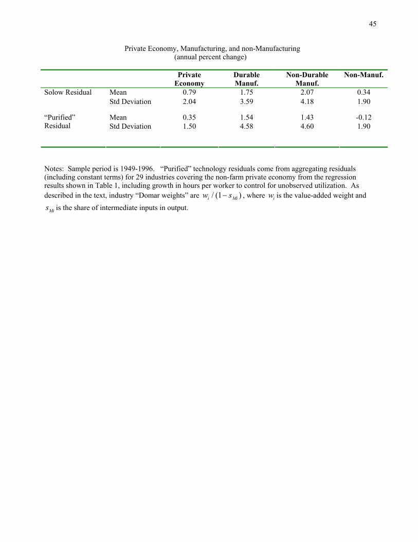
45

Private Economy, Manufacturing, and non-Manufacturing (annual percent change)

Private

Economy Durable Manuf.

Non-Durable Manuf.

Non-Manuf.

Mean 0.79 1.75 2.07 0.34 Solow Residual

Std Deviation 2.04 3.59 4.18 1.90

Mean 0.35 1.54 1.43 -0.12 “Purified” Residual

Std Deviation 1.50 4.58 4.60 1.90

Notes: Sample period is 1949-1996. “Purified” technology residuals come from aggregating residuals (including constant terms) for 29 industries covering the non-farm private economy from the regression results shown in Table 1, including growth in hours per worker to control for unobserved utilization. As described in the text, industry “Domar weights” are w si / ( )1 Mi− , where is the value-added weight and iw

Mis is the share of intermediate inputs in output.

46

Table 3: Regressions on Current and Lagged Technology

Regressor Dependent Variable (Growth rate, unless otherwise indicated)

dz dz(-1) dz(-2) dz(-3) dz(-4) R2 DW Stat.

0.00 1.17 0.52 -0.08 -0.48 0.43 2.39 (1) Output (0.21) (0.34) (0.2) (0.21) (0.2)

-0.60 0.55 0.51 -0.06 -0.41 0.45 1.70 (2) Hours (0.14) (0.27) (0.12) (0.16) (0.19)

-0.44 0.40 0.43 0.08 -0.21 0.48 1.45 (3) Input (0.09) (0.17) (0.07) (0.12) (0.12)

-0.40 0.68 0.06 -0.26 -0.23 0.53 2.81 (4) Utilization (0.13) (0.15) (0.16) (0.12) (0.09)

-0.52 0.36 0.48 0.11 -0.34 0.42 1.56 (5) Employment (0.11) (0.25) (0.09) (0.15) (0.18)

0.44 0.76 0.09 -0.16 -0.27 0.46 2.94 (6) TFP (Solow residual) (0.15) (0.2) (0.17) (0.13) (0.11)

-1.07 1.04 1.63 -0.20 -0.81 0.35 1.43 (7) Non-residential fixed investment (0.36) (0.79) (0.43) (0.42) (0.61)

1.25 2.83 -0.07 -1.70 -1.36 0.44 2.20 (8) Resid investment and cons. durables (0.5) (0.89) (0.67) (0.47) (0.58)

0.10 0.41 0.24 0.03 -0.14 0.40 1.79 (9) Consumer Non-Dur and Services (0.11) (0.11) (0.1) (0.08) (0.09)

-0.14 0.11 0.14 0.04 -0.02 0.42 1.60 (10) ∆ Inventories/GDP (not in growth rates)

(0.03) (0.05) (0.04) (0.05) (0.04)

0.01 -0.03 0.07 0.19 0.20 0.16 0.29 (11) Net Exports/GDP (not in growth rates

(0.13) (0.13) (0.1) (0.1) (0.11) Notes: Each row represents a separate OLS regression of the variable shown (in growth rates, unless otherwise indicated) on the current value plus four lags of estimated technology growth, plus a constant term (not shown). Heteroskedasticity- and autocorrelation-robust standard errors in parentheses (calculated with TSP’s GMM command with NMA=3). All regressions are estimated from 1953-1996. (master_subper_2.4.10lags.xls)

47

Table 4. Fraction of Variance Due to Technology Shocks

Lags Output Inputs Hours Utilization Solow Res.

0 0 28 21 23 18

1 19 13 10 20 56

3 43 13 9 17 70

10 51 11 7 11 76

Notes: Variance decomposition from bivariate VAR of technology and the variable shown.

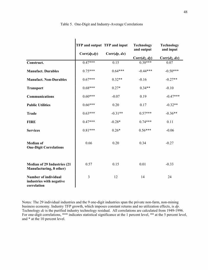
48

Table 5. One-Digit and Industry-Average Correlations

TFP and output

Corr(dp,dy)

TFP and input

Corr(dp, dx)

Technology and output

Corr(dz, dy)

Technology and input

Corr(dz, dx)

Construct.

0.47*** 0.15 0.38*** 0.07

Manufact. Durables

0.75*** 0.64*** -0.44*** -0.50***

Manufact. Non-Durables

0.67*** 0.32** -0.16 -0.27**

Transport

0.68*** 0.27* 0.34** -0.10

Communications

0.60*** -0.07 0.19 -0.47***

Public Utilities

0.66*** 0.20 0.17 -0.32**

Trade

0.63*** -0.31** 0.57*** -0.36**

FIRE

0.47*** -0.28* 0.74*** 0.11

Services

0.81*** 0.26* 0.56*** -0.06

Median of One-Digit Correlations

0.66 0.20 0.34 -0.27

Median of 29 Industries (21 Manufacturing, 8 other)

0.57 0.15 0.01 -0.33

Number of individual industries with negative correlation

3 12 14 24

Notes: The 29 individual industries and the 9 one-digit industries span the private non-farm, non-mining business economy. Industry TFP growth, which imposes constant returns and no utilization effects, is dp. Technology dz is the purified industry technology residual. All correlations are calculated from 1949-1996. For one-digit correlations, *** indicates statistical significance at the 1 percent level, ** at the 5 percent level, and * at the 10 percent level.

49

Table 6. Responses by sub-period

dt dt(-1) dt(-2) dt dt(-1) dt(-2)Output -0.10 1.14 1.03 0.33 1.18 0.00 0.47 2.37

(0.31) (0.39) (0.26) (0.19) (0.52) (0.25)

Hours -0.62 0.50 0.91 -0.29 0.77 0.32 0.50 1.72(0.2) (0.34) (0.16) (0.16) (0.34) (0.11)

Nonresidential Investment -0.65 1.28 2.81 -1.31 0.65 0.62 0.40 1.51(0.51) (0.82) (0.46) (0.49) (1.25) (0.69)

Nonfarm Business Deflator -1.03 -0.80 -0.50 -0.87 -0.57 -0.06 0.83 1.59(0.15) (0.22) (0.15) (0.22) (0.07) (0.13)

Real Fed Funds 0.14 0.06 0.15 -0.48 -0.60 -0.48 0.77 1.74(0.19) (0.2) (0.16) (0.22) (0.1) (0.14)

1949-1979 1980-1996R2 DW

Statistic

Notes: Coefficients from bivariate regressions of the growth rate of the variable shown on current and two lags of purified technology growth, dz. The coefficients are allowed to differ by subperiod. All regressions include decadal dummies (the 1970s dummy is important for the nonfarm business deflator; the 1980s dummy is important for the real fed funds rate). Heteroskedasticity- and autocorrelation-robust standard errors in parentheses. sub2lags-5.xls

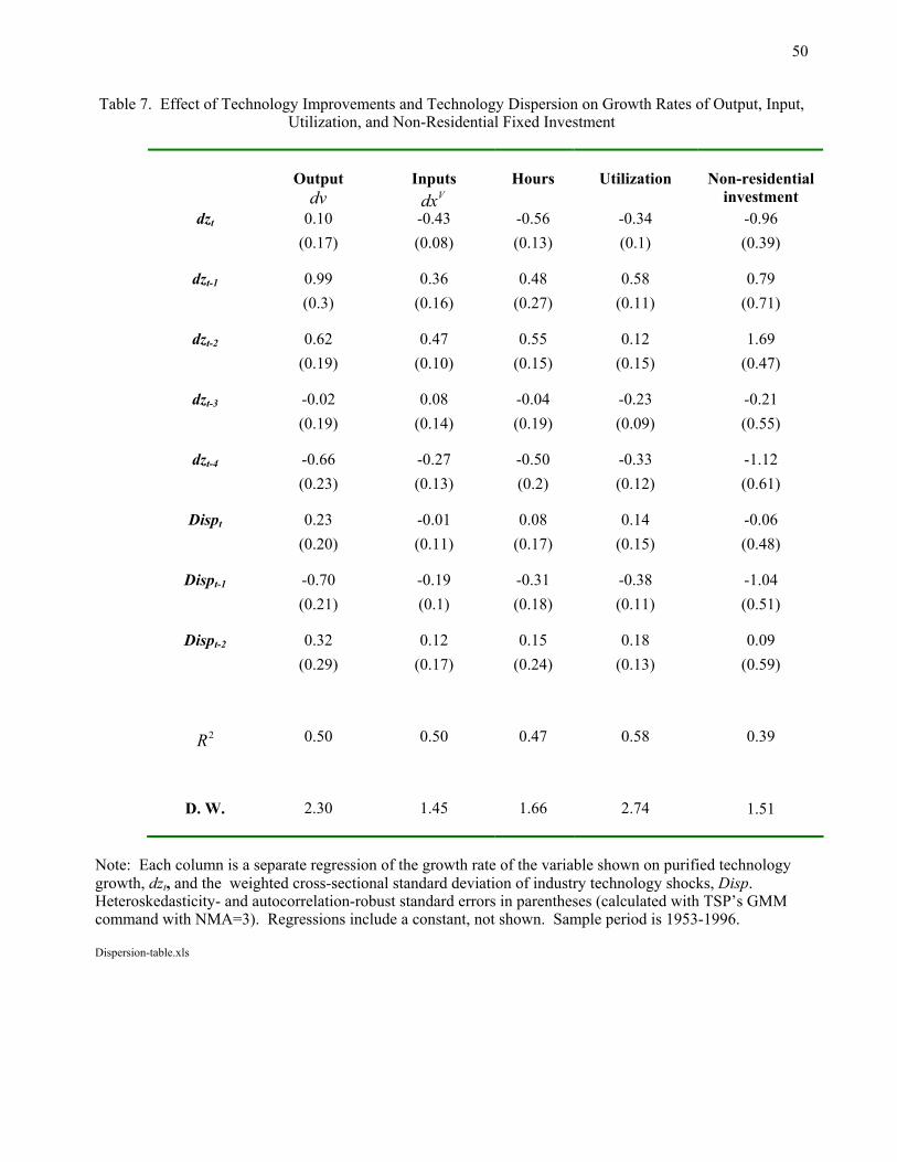
50

Table 7. Effect of Technology Improvements and Technology Dispersion on Growth Rates of Output, Input, Utilization, and Non-Residential Fixed Investment

Output dv

Inputs

dxV

Hours

Utilization

Non-residential

investment 0.10 -0.43 -0.56 -0.34 -0.96 dzt

(0.17) (0.08) (0.13) (0.1) (0.39)

0.99 0.36 0.48 0.58 0.79 dzt-1 (0.3) (0.16) (0.27) (0.11) (0.71)

0.62 0.47 0.55 0.12 1.69 dzt-2 (0.19) (0.10) (0.15) (0.15) (0.47)

-0.02 0.08 -0.04 -0.23 -0.21 dzt-3 (0.19) (0.14) (0.19) (0.09) (0.55)

-0.66 -0.27 -0.50 -0.33 -1.12 dzt-4 (0.23) (0.13) (0.2) (0.12) (0.61)

0.23 -0.01 0.08 0.14 -0.06 Dispt

(0.20) (0.11) (0.17) (0.15) (0.48)

-0.70 -0.19 -0.31 -0.38 -1.04 Dispt-1

(0.21) (0.1) (0.18) (0.11) (0.51)

0.32 0.12 0.15 0.18 0.09 Dispt-2

(0.29) (0.17) (0.24) (0.13) (0.59)

0.50 0.50 0.47 0.58 0.39 R2

D. W.

2.30 1.45 1.66 2.74 1.51

Note: Each column is a separate regression of the growth rate of the variable shown on purified technology growth, dzt, and the weighted cross-sectional standard deviation of industry technology shocks, Disp. Heteroskedasticity- and autocorrelation-robust standard errors in parentheses (calculated with TSP’s GMM command with NMA=3). Regressions include a constant, not shown. Sample period is 1953-1996. Dispersion-table.xls

51

Figure 1. TFP, Output, and Hours (Annual percent change)

50 55 60 65 70 75 80 85 90 95

-6

-4

-2

0

2

4

6

Percentage pointsTFP Output Hours worked

Notes: All series are demeaned. Sample period is 1949-96. All series cover the non-farm, non-mining private business economy. Growth in aggregate output is measured as real value added. Growth in inputs is measured as the share-weighted average of growth in primary inputs of capital and labor. TFP is measured as output growth minus input growth. Shaded regions show NBER recession dates.

52

Figure 2. Technology, TFP, Output, Hours, Utilization, and Non-Residential Investment (Annual percent change)

50 55 60 65 70 75 80 85 90 95

0

5 Technology TFP

50 55 60 65 70 75 80 85 90 95

-5

0

5 Technology Output

50 55 60 65 70 75 80 85 90 95

-5

0

5

Percentage points

Technology Hours

50 55 60 65 70 75 80 85 90 95

-2.5

0.0

2.5

5.0 Technology Utilization

50 55 60 65 70 75 80 85 90 95

-15

-10

-5

0

5

10Technology Non-residential investment

Notes: All series are demeaned. Sample period is 1949-96. All series cover the non-farm, non-mining private business economy. Technology is the utilization-corrected aggregate residual. For description of series, see text and/or notes to Figure 1 and Table 2. Shaded regions show NBER recession dates.

Fig-2-dtcon-4-panel.gwg and investment-and-technology-like-5-panel.gwg

53

Figure 3. Impulse Responses to Technology Improvement: Quantities

Output

-1.0

-0.5

0.0

0.5

1.0

1.5

2.0

2.5

0 1 2 3 4 5 6 7 8 9 10

Perc

enta

ge P

oint

s

Hours

-1.5

-1.0

-0.5

0.0

0.5

1.0

1.5

0 1 2 3 4 5 6 7 8 9 10

Perc

enta

ge P

oint

s

Input

-1.0

-0.5

0.0

0.5

1.0

1.5

0 1 2 3 4 5 6 7 8 9 10

Perc

enta

ge P

oint

s

Utilization

-1.0

-0.5

0.0

0.5

1.0

0 1 2 3 4 5 6 7 8 9 10

Perc

enta

ge P

oint

s

I

Employment

-1.0

-0.5

0.0

0.5

1.0

1.5

0 1 2 3 4 5 6 7 8 9 10

Perc

enta

ge P

oint

sSolow Residual

0.0

0.5

1.0

1.5

2.0

0 1 2 3 4 5 6 7 8 9 10

Perc

enta

ge P

oint

s

Nonresidential Investment

-3.0

-1.5

0.0

1.5

3.0

0 1 2 3 4 5 6 7 8 9 10

Perc

enta

ge P

oint

s

Durables + Residential Investment

-1.5

0.0

1.5

3.0

4.5

6.0

0 1 2 3 4 5 6 7 8 9 10

Perc

enta

ge P

oint

s

Nondurables + Services

-0.5

0.0

0.5

1.0

1.5

0 1 2 3 4 5 6 7 8 9 10

Perc

enta

ge P

oint

s

Change in Inventories/GDP

-0.5

-0.3

0.0

0.3

0.5

0 1 2 3 4 5 6 7 8 9 10

Perc

enta

ge P

oint

s

Net Exports/GDP

-1.0

-0.5

0.0

0.5

1.0

1.5

0 1 2 3 4 5 6 7 8 9 10

Perc

enta

ge P

oint

s

Note: Impulse responses to a 1 percent improvement in “purified” technology, estimated from bivariate VARs where purified technology is taken to be exogenous. All entries are percent changes; horizontal scale represents years after the technology shock. Dotted lines show 95 percent confidence intervals, computed using RATS Monte Carlo method. Sample period is 1952-96. Figs34_shortrun_IRs_with_dtcon2_5.17.xls

54

Figure 4. Impulse Responses to Technology Improvement: Prices and Interest Rates

Nonfarm Business GDP Deflator

-2.0

-1.5

-1.0

-0.5

0.0

0 1 2 3 4 5 6 7 8 9 10

Perc

enta

ge P

oint

s

Investment + Durables Deflator

-3.0

-1.5

0.0

1.5

0 1 2 3 4 5 6 7 8 9 10

Perc

enta

ge P

oint

s

y

Nondurables + Services Deflator

-3.0

-1.5

0.0

0 1 2 3 4 5 6 7 8 9 10

Perc

enta

ge P

oint

s

Relative Price Deflator

-0.5

0.0

0.5

1.0

0 1 2 3 4 5 6 7 8 9 10

Perc

enta

ge P

oint

s

Nominal Fed Funds Rate

-1.5

-1.0

-0.5

0.0

0.5

1.0

0 1 2 3 4 5 6 7 8 9 10

Perc

enta

ge P

oint

sNominal 3-Month Treasury Bill

-1.0

-0.5

0.0

0.5

0 1 2 3 4 5 6 7 8 9 10

Perc

enta

ge P

oint

s

Real Fed Funds Rate

-1.0

-0.5

0.0

0.5

0 1 2 3 4 5 6 7 8 9 10

Perc

enta

ge P

oint

s

Real 3-Month Treasury Bill

-1.0

-0.5

0.0

0.5

0 1 2 3 4 5 6 7 8 9 10

Perc

enta

ge P

oint

s

Real Exchange Rate

-20

-15

-10

-5

0

5

0 1 2 3 4 5 6 7 8 9 10

Perc

enta

ge P

oint

s

Real Wage

0.0

0.4

0.8

1.2

1.6

2.0

0 1 2 3 4 5 6 7 8 9 10

Perc

enta

ge P

oint

s

Nominal Exchange Rate

-20

-15

-10

-5

0

5

10

0 1 2 3 4 5 6 7 8 9 10

Perc

enta

ge P

oint

s

Nominal Wage

-1.5

-1.0

-0.5

0.0

0.5

1.0

1.5

0 1 2 3 4 5 6 7 8 9 10

Perc

enta

ge P

oint

s

Note: Impulse responses to 1 percent improvement in “purified” technology, estimated from bivariate VARs where purified technology is taken to be exogenous. All entries are percent changes; horizontal scale represents years after the technology shock. VARs for prices, interest rates, and wages include decadal dummy variables for 1970s and 1980s. For nominal and real trade-weighted exchange rate, an increase represents an appreciation. Investment includes residential and non-residential investment; relative price deflator is ratio of deflator for investment (residential and non-residential) and consumer durables to the price deflator for consumer non-durables and services. Dotted lines show 95 percent confidence intervals, computed using RATS Monte Carlo method. Sample period is 1952-96 except for the fed funds rate (1957-96) and real/nominal exchange rate (1973-96). Figs34_shortrun_IRs_with_dtcon2_5.17.xls

55

Figure 5. Alternative estimates of the hours and investment response to a technology improvement

Short Run Impulse Responses for Hours

-1.5

-1

-0.5

0

0.5

1

1.5

0 1 2 3 4 5 6 7 8 9

(1) Implied response from regressing hours on current and 10 lags of technology

(6) Using BLS hours (levels) allowing feedback

(5) Using BLS hours (differences) allowing feedback

(4) Allowing for serial correlation and feedback

(2) Benchmark VAR: Not allowing for serial correlation or feedback

(3) Allowing for serial correlation but no feedback

10

Percentage points

Srhours_dtcon.xlsYears

Short Run Impulse Responses for Nonresidential Investment

-2

-0.5

1

2.5

0 1 2 3 4 5 6 7 8 9

(1) Implied response from regressing hours on current and 10 lags of technology

(4) Allowing for serial correlation and feedback

(2) Benchmark VAR: Not allowing for serial correlation or feedback

(3) Allowing for serial correlation but no feedback

10

Srnonres_dtcon-1.xls Notes: Each line represents the impulse response from a separate estimation. For all specifications shown, the impact effect (year 0) is statistically significantly negative. (1) is cumulated response from regressions on current and 10 lags of technology; sample period is 1959-1996. (2)-(6) are from bivariate VARs with two lags, estimated 1951-1996. (2) does not allow serial correlation or feedback in the equation for purified technology; (3) allows serial correlation; (4)-(6) allow serial correlation and feedback. In top panel, (1)-(4) use aggregate hours growth from Jorgenson dataset; (5) and (6) use growth and log-level of BLS nonfarm business hours per capita (aged 16 and older).

56

Figure 6. Estimates from a VAR with long-run restrictions: Hours response to a technology improvement

Levels Differences

0 1 2 3 4 5 6 7 8 9 10-1.5

-1

-0.5

0

0.5

1

1.5

2

0 1 2 3 4 5 6 7 8 9 10

-1.5

-1

-0.5

0

0.5

1

1.5

Percentage points

Notes: Responses identified from the assumption that only “true” technology affects the level of purified technology in the long run. Response shows percentage-point deviation of the level of hours; horizontal scale represents years after the technology shock.. The “level” specification uses the log-level of hours worked from Jorgenson dataset (private non-farm, non-mining business) divided by the population aged 16 and older. The difference specification uses the growth rate of hours worked per capita. 95 percent confidence interval shown.