naval postgrauuate school monterey, california naval postgrauuate school monterey, california a...
TRANSCRIPT

COPy
NAVAL POSTGRAUUATE SCHOOLMonterey, California
A D)OTICELECTEfft
MARO 81990 THESIS B
REAL TIME MARINE GAS TURBINE
SIMULATION FOR ADVANCED CONTROLLERDESIGN
by
Stephen D. Metz
September 1989
Thesis Advisor: David L. Smith
Approved for Public release; distribution unlimited.
....0I II • : ii-

UNCLASSIFIEDSECUR!TY CLASSIFICATION OF THIS PAGE
REPORT DOCUMENTATION PAGEla REPORT SECURITY CLASSIFICATION ib RESTRICTIVE MARKINGS
UNCLASSIFIED2a SECURITY CLASSIFICATION AUTHORITY 3 DISTRIBUTION 'AVAILABILITY OF REPORT
Approved for Public release;2b DECLASSIFICATION, DOWNGRADING SCHEDULE distribution is unl imi ted.
4 PERFORMING ORGANIZATION REPORT NUMBERIS) 5 MONITORING ORGANIZATION REPORT NUMBER(S)
6a NAME OF PERFORMING ORGANIZATION 6b OFFICE SYMBOL 7a. NAME OF MONITORING ORGANIZATION(If applicable)
Naval Postgraduate School Code 69 Naval Postgraduate School
6c ADDRESS (City, Stare, and ZIP Code) 7b. ADDRESS (City, State, and ZIP Code)
Monterey, California 93943-5000 Monterey, California 93943-5000
8a NAME OF FUNDING/SPONSORING 8b OFFICE SYMBOL 9 PROCUREMENT INSTRUMENT IDENTIFICATION NUMBERORGANIZATION (If applicable)
Naval Postgraduate School I
8c ADDRESS (City, State, and ZIP Code) 10. SOURCE OF FUNDING NUMBERSPROGRAM PROJECT TASK WORK UNIT
Monterey, California 93943-5000 ELEMENT NO NO NO ACCESSION NO
11 TITLE (Include Security Classification)
Real Time Marine Gas Turbine Simulation for Advanced Controller Design12 PERSONAL AUTHOR(S)
Metz, Stephen U.
13a YPEOF EPOR jFROTME COEETO ~ DT OF REPORT (Year, Month, Day) 5 PAGFCU,Masters Thesis 7 RMT 89 September16 SUPPLEMENTARY NOTATION Views expressed in this thesis are of the author and do not reflect
the official policy or position of the Department of Defense or the U.S. Government.
17 COSATI CODES 18 SUBJECT TERMS (Continue on reverse if necessary and identify by block number)
FIELD GROUP SUB-GROUP -,Marine Gas Turbine Modeling Gas Turbine Control
19 ABSTRACT (Continue on reverse if necessary and identify by block number)
The Marine Gas Turbine control systems in present use in the US Navy are of such significant technologicalage that new design techniques could lead to more optimal performance and increased plant efficiency. Tothis end, a new real time Marine Gas Turbine simulation method is needed for advanced controller designand implementation.
A modeling method is shown which utilizes real time sequential linearizations to approximate the truenonlinear response of the NPS Boeing 502-6A test facility. A validation of this simulation approach ispresented. The method has immediate application to advanced controller design, especially to the designof modern regulators (Linear Quadratic), model reference controllers, and real time diagnostics.
20 DISTRIBUTION 'AVAILABILITY OF ABSTRACT 21 ABSTRACT SECURITY CLASSIFICATION
t UNCLASSIFIED/UNLIMITED 0 SAME AS RPT Q DTIC USERS UNCLASSIFIED22a NAME OF RESPONSIBLE iNDIVIDUAL 22b TELEPHONE (Include Area Code) z2c OFFICE SYMBOLProf. David L. Smith (408)646-0448 Cnd 6qSm
DD FORM 1473, 84 MAR 83 APR edition may be used unti, exhausted SECURITY CLASSIFICATION OF THIS PAGEAll other editions are obsolete U . G o w O 1 P
I Oe~ etIl'tnlO t€ ! 1-40 .4
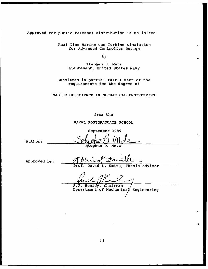
Approved for public release; distribution is unlimited
Real Time Marine Gas Turbine Simulationfor Advanced Controller Design
by
Stephen D. MetzLieutenant, United States Navy
Submitted in partial fulfillment of therequirements for the degree of
MASTER OF SCIENCE IN MECHANICAL ENGINEERING
from the
NAVAL POSTGRADUATE SCHOOL
September 1989
Author: et k,tephen D. Metz
Approved by:__Prof. David L. Smith, Thesis Advisor
Department Yof Chan caEngineering

The Marine Gas Turbine control systems in present use in the U. S.Navy are of such significant technological age that new design
techniques could lead to more optimum performance and increased
plant efficiency. To this end, a new real time Marine Gas Turbine
simulation method is needed for advanced controller design and
implementation.
A modeling method is shown which utilizes real time sequentiallinearizations to approximate the true nonlinear response of the NPS
Boeing 502-6A test facility. A validation of this simulation approach is
presented. The method has immediate application to advanced
controller design, especially to the design of modern regulators
(Linear Quadratic), model reference controllers, and real time
diagnostics.
Accession
NTIS GRA&IDTtC TAB 0Unnnnounced 0Ju;itl!f ont lon
f ... I- -
V 7 Distribuation/_____
- A'Id1lfbflil.' CV,%A 0
iii I

TABLE OF CONTENTS
I. IN TR O D U CTIO N ........................................................................................... 1
II. PAST WORK IN GAS TURBINE MODELING .................................... 2
III. MODEL STRUCTURE AND COARSE TUNING .................................. 7A. ModelingB. State selectionsC. Steady componentsD. Dynamic componentsE. Linearized dynamic equation setF. Decoupling the equation set
IV. FINE TUNING THE MODEL ................................................................ 25
A. Computer simulationB. Grid search
V. VALIDATION OF THE MODEL ............................................................ 30
VI. CO NCLUSIO NS ......................................................................................... 36
APPENDIX A: COMPONENT MODELING EQUATIONS ..................... 40
APPENDIX B: EQUATION SET REDUCTION METHODOLOGY ........ 43
APPENDIX C: PARAMETER SELECTION METHODOLOGY ............... 48
APPENDIX D: COMPUTER SIMULATION CODES .............................. 52
APPENDIX E: SOURCE DATA RUNS ....................................................... 68
LIST OF REFERENCES ............................................................................. 74
INITIAL DISTRIBUTON U1ST .................................................................. 75
iv

LIST OF TABLS
1. Data ------------------------------------------------ 12
2. Normalization Points ----------------------------------- 13
3. Component Equations ------------------------------------------------ 14
4. Steady and Dynamic Components ------------------------ 16
5. Dynamic Equation Set -------------------------------------------------- 19
9.v
.. . ... ,,mm , mmmmmmmmmmm mm m lmmm m m mmm mm m m l m llV
LIST OF FIGURES
1. Multiport Diagram ------------------------------------------------------- 52. Test Bed Configuration ------------------------------------------ 83. Gas Turbine Components ---------------------------------------------- 94. Compressor Block Diagram -------------------------------------------- 105. Gas Turbine Operating Range ----------------------------------------- 116. P2 and P4 Graphical Representations ------------------------------ 21
7. Sequential Linearization ----------------------------------------------- 268. Simulation Process ----------------------------------------------------- 26
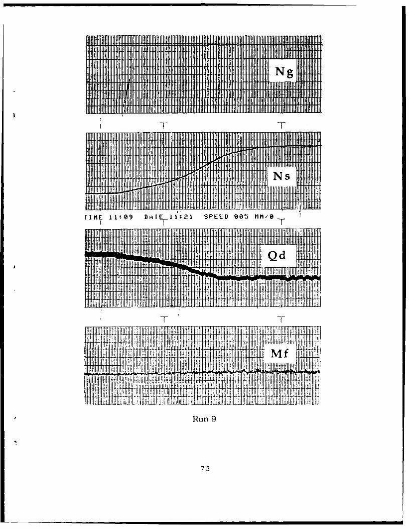
9. Dynamic DaLa ui-s ----------------------------------------------------- 2910. Simulation-Run Nine -------------------------------------------------- 31
11. Validation-Run One ---------------------------------------------------- 3212. Simulation-Run Three ------------------------------------------------ 34
13. Validation-Run Seven ------------------------------------------------- 35
vi

LIST OF YY M OQ ANnABBREIATIONS
E - Fuel Combustion Energy Realized at HP Turbine
JD - Dynamometer Torque
JG - Gas Generator Torque
Ma - Mass Flowrate of Air
Maf - Mass Flowrate of Air/Fuel Mixture
Mf - Mass Flowrate of Fuel
Ng - Gas Generator Speed
Ns - Power Turbine/Dynamometer Speed
Qc - Compressor Torque
Qd - Dynamometer Torque
Qfpt - Free Power Turbine Torque
Qhpt - High Pressure Turbine Torque
P2 - Compressor Discharge Pressure
P4 - High Pressure Turbine Discharge Pressure
T2 - Compressor Discharge Temperature
T4 _ High Pressure Turbine Discharge Temperature
Note: 1. Lower case variables represent normalized
variables.
2. _B denotes normalizing values. (i.e. JGB, NGB,
QCB, etc.)
vii

ACKNOWLEDGEMENTS
The author would like to express his appreciation to his wife for the
understanding, patience, and support shown throughout the entire
Masters degree program. A special thanks also goes out to Professor
David Smith whose eternal optimism and encouragement helped to
keep this researcher on track.
viii

1. INTRODUCTION
Conventional control theory is limited to time invariant single-input-
single-output systems and is u,.ually based on a frequency domain
design approach. Modem control theory, on the other hand, can be
well applied to multiple-input-multiple-output, non-linear gas turbine
systems which are now in use and it relies on a much more applicable
time doi,,ain approach.l The feasibility of modern control theory
such as Linear Quadratic Regulator (LQR) theory, in the application of
marine gas turbines for propulsion has been demonstrated by past
work at the Naval Postgraduate School in Monterey, Califomia. 2 - 4 For
this application to be successful a simple, accurate, and robust real
time marine gas turbine simulation must be developed.
This thesis introduces a modeling approach to be applied in
developing a real time simulation of engine response to meet the
requirements of simplicity, accuracy, and robustness. It is simple in
that it is only first order dependent, accurate in that it prow'des
acceptable (+/- 10%) response for use in application of advanced
engine control design. and robust in that it wo~ks well over the entire
operational range of the gas turbine system.
• .. . i I I I ! I I

I. PAST WORK IN GAS TURBINE MODELING
Past work in Gas Turbine Modeling is discussed in terms of two
areas: first, a brief discussion on gas turbine modeling in general is
presented. This is followed by a discussion on the previous work
completed at the Naval Postgraduate School in Monterey, California.
Since most marine gas turbines have been derived from aviation
sources, most of the early gas turbine modeling work was
accomplished in the aviation arena. In the 1970's the Naval Gas
Turbine Ship Propulsion Dynamics and Control Systems Research and
Development Program was started to address the issues of designing
Marine Gas Turbines for future use in the Navy.5 This included the
dynamic modeling of the response of , marine gas turbine. Prior to
this program, most of the work had been steady state modeling.
However, the Navy realized that dynamic modeling was needed for
advanced controller design. The program was successful in developing
a gas turbine machinery dynamics and control system data base. From
this work a computer-based propulsion control testbed was developed
for use in gas turbine controller development. Cut and try linear
control design then ensued, which resulted in a gain adjusted
2

controller design in use in today's fleet. This approach resulted in a
linear Proportional-Integral theory being applied to a nonlinear
system. The results were deemed adequate for the Navy's uses.
A new approach to this modeling is to develop a method -,o
accurately model the propulsion plant nonlinear responses with a real
time simulator. This would help eliminate or alleviate problems
associated with the varying propeller loads felt in the gas turbine by
predicting the responses before they actually occur, thus allowing
more acurate control. More accurate control would mean better
engine response to these loads and would, in turc:, mean less wear,
thus leading to longer engine life as well as better engine fuel
efficiency. This i5 the direction taken at the Naval Postgraduate
School, (NPS), in the gas turbine modeling problem.
The previous work started with Phillip Johnson in 1985 in which
he conducted the development and implementation of a load control
system ( e.g. a water brake dynamometer) to emulate the shaft and
propeller of a marine gas turbine. 6 The next step was taken by James
Roger also in 1985. He used a simple multiport diagram and the
Continous System Modeling Program (CSMP III) to incorporate an
3

improved model for the dynamometer unloading valve into the existing
system dynamic model. 7 These two works formed the base for the
next step performed by Vincent Herda in 1986. Herda developed a
better multiport model and used it to develop a linear state space
model and a nonlinear dynamic propulsion model. 2 Robert Miller
followed in the same year using Herda's models and examined the
feasibility of using Linear Quadratic Regulator (LQR) control design
theory for a small gas turbine, specifically the Boeing 502-6A test bed
installation at NPS. 3 Finally Vincent Stammetti in 1988 developed the
first real time dynamic simulator for the gas turbine and compared an
LQR controller to a classical Proportional Integral (PI) regulator based
on his results with the simulator.4 To summarize, Herda validated
cause and effect through the use of his new multiport model, shown in
figure 1 , Miller validated the steady-state model method and
Stammetti followed with the first linear model structure. It is
important to note that these models were only accurate for one run
of simulation and were not applicable over the whole range of
operation of the gas turbine. Their main point however, was to
validate and show the feasibility of developing a better model for use in
modem controller design to update those in current use today. To
this end they were successful. This paper will continue this work and
attempt to develop a simple, robust, and accurate real time marine gas
4

Cr)z4
0
tA',
Cy~
to
5x

turbine simulator to be used for advanced controller design.
I8

M. MODEL STRUCTURE AND COARSE TUNIN
A. Modeling
The gas turbine plant to be modeled was the 175 horsepower
Boeing 502-6A which was assembled in a test bed configuration at the
Naval Postgraduate School in Monterey, California. It was coupled to a
Clayton 17-300 water brake dynamometer which was used to simulate
the shaft and propeller loading on a marine gas turbine. The gas
turbine/water brake assembly is shown in figure 2. The gas turbine
itself was composed of two aerodynamically coupled sections, a gas
generating section and a power output section. The gas generator had
three major components. These were the compressor, the burner,
and the high pressure turbine shown in figure 3. Connected by
gearing off the gas generator shaft was the accessory section
consisting of the fuel pump, lube oil pump, governor, tachometer
generator, and the starter. The compressor was a single stage
centrifugal compressor and was coupled to the high pressure turbine
aerodymanically via two through-flow type, cross-connected
combustion chambers. The high pressure turbine was a single stage
axial flow high pressure turbine. It was aerodynamically connected to
the low pressure or free power turbine which was also an axial flow
turbine. The free power turbine output shaft was mechanically
coupled to the water brake dynamometer which absorbs the energy of
7

shaftgas speed water
turbine sensor dynomometer
Inlet
sensors
Figure 2. Test Bed Configuration.
175 Hp Boeing 502-6A gas turbine
Single stage centrifugal compressor
Two single stage axial turbines
Clayton 17-300 water brake dynamometer
Assorted sensors
Pressure
Temperature
Output torque
Rotational speeds
Fuel flow rate
8

I-
0
zzv0
lu 100
Ch
CCVz(
0-b0iEri
9L
IMI

the free power turbine in simulating the action of a drive shaft and
propeller.
The modeling began with Herda's cause and effect multiport
diagram shown in figure 1. The importance of this diagram to the
method can hardly be overstated. Each of the components, the
compressor, high pressure and free power turbines, and the gas
generator and dynamometer shafts, were modeled by describing their
outputs in terms of their inputs in equation form. For example, the
compressor inputs are gas generator speed (Ng) and the high pressure
turbine inlet pressure (P2) and the outputs are mass flow rate of air
(Ma), high pressure turbine inlet temperature (T2), and compressor
torque (Qc). The compressor block diagram is shown in figure 4.
-- p Ma
Compressor T2
P2 Figure 4. Compressor Block Diagram.
1 7*It is important to note that these input/output quantities as well as
those for the other components must be measurable or calculable.
They were recorded and or calculated over the operating range of the
gas turbine (shown in figure 5), and the results are tabulated In table
1. For clarity, the operating region of the turbine is shown in figure 5.
10

32000 x -x
29000
TURBINE
NG OPERATING
26000 A E(RPM)
23000
20000 X xx
500 1000 1500 2000 2500
NS (RPM)
Figure 5. Gas Turbine Operating Range.

Ng Ns Qd/ T2 F2 T4 r4 Mf Ma Qc/Qfpt QhPt
rpm - rpm-ftlbf--f -- psig - f--psig-lbm/hr-lbm/s-ftlbf--------------------------------------------------..----
20040 500 125 146. 73 6. 63 868 .85 76. 98 1. 73 60. 56420020 1003 95 146.68 6.68 882 .94 78 39 1.71 60.98120000 1504 70 146.90 6.70 880 .96 79.40 1.71 62.76419930 2002 40 147.15 6.75 876 .95 79-40 1.771 63.32620000 2267 20 146. 93 6. 60 878 .90 79. 40 1. 71 64. 02023050 511 180 177. 45 9. 18 877 1. 15 91. 45 2.05 65. 69623060 1009 145 177.20 9.25 902 1.30 94.49 2.03 67. 45523060 1500 115 176.15 9.40 902 1.35 94.98 2.03 69.32923160 2008 80 175.30 9.35 895 1.35 94.98 2.03 70.43923020 2509 40 174.98 9.33 897 1.30 94.98 2.01 72.43426010 506 245 205.90 12.20 886 1.59 108.31 2.42 72.82826090 1006 200 206.58 12.55 922 1.72 110.83 2.38 71.37826080 1502 170 208.03 12.43 917 1.80 113.60 2.35 74. 23826090 2000 130 207.40 12.55 921 1.90 113.60 2.35 76. 30626090 2510 100 208.50 12.55 926 1.85 113.60 2.36 75.66729020 509 320 244. 18 16.05 913 2. 10 128. 67 2. 74 85. 80229060 1010 280 247.33 16.05 960 2.20 131.44 2.69 80.09529010 1504 230 245.85 16.35 967 2.40 135.47 2.67 78. 71129050 2000 195 244. 36 16. 45 970 2. 50 136. 47 2. 66 81. 16729060 2515 160 242. 40 16. 40 956 2. 50 137. 24 2. 66 85 73632030 509 420 280. 65 20. 50 978 2. 70 157. 84 3.06 99. 81032020 1010 365 283.03 20.80 1002 2.85 161.86 3.03 94.68532020 1510 310 281.05 20.90 1039 3.00 165.11 3.01 90.22132010 2017 275 283. 50 20.95 1024 3. 30 167.60 3.04 91. 63432000 2510 240 284. 70 20. 85 1044 3. 30 168. 34 2. 99 89. 646
(A)
ng ns qd/qfpt 12 p2 14 p4 Mf Ma qc/c*Vt maf
0.77077 0.33333 0.56818 0.68247 0.47357 0.90795 0.44737 0.62841 0.73305 0.75705 0.723710.77000 0.66867 0.43182 0.68223 0.47714 0.92259 0.49474 0.63992 0.72458 0.76226 0.715610.76923 1.00267 0.31818 0.68326 0.47857 0.92050 0.50526 0.64816 0.72458 0.78455 0.715730.76654 1.33467 0.18182 0.68442 0.48214 0.91632 0.50000 0.64816 0.72458 0.79157 0.715730.76923 1.51133 0.09091 0.68340 0.47143 0.91801 0.47368 0.6A816 0.72q58 0.80025 0.715730.88654 0.34067 0.81818 0.82535 0.65571 0.91736 0.60526 0.74653 0.86864 0.82120 0.857600.88692 0.67Z67 0.65909 0.8Z419 0.66071 0.94351 0.68421 0.7713S 0.86017 0.84319 0.849690.88692 1.00000 0.52273 0.81930 0.67143 0.94351 0.71053 0.77535 0.86017 0.86661 0.849750.89077 1.33867 0.36364 0.81535 0.66786 0.93619 0.71053 0.77535 0.86017 0.8804- 0.840750.88538 1.67267 0.18182 0.81386 0.66643 0.93828 0.68421 0.77535 0 ?5169 0.90542 0.841481.00038 0.33733 1.11364 0.95767 0.87143 0.9Z678 0.811-e4 0.88416 1.02542 0.91035 1.012431.00346 0.67067 0.90909 0.96084 0.89641 0.16444 0.90526 0.90473 1.008047 0.89222 0.996191.00308 1.00133 0.77273 0.96758 0.88786 0.95920 0.94737 0.92735 0.99576 0.92797 0.984111.00346 1.33333 0.59091 0.96465 0.89643 0.96339 1.00000 0.92735 0.99576 0.95382 0.984111.00346 1.67333 0.45455 0.96977 0.89643 0.96862 0.97368 0.92735 1.00000 0.94584 0.$88251.11615 0.33933 1.45455 1.13572 1.14643 0.95502 1.10526 1.05037 1.16102 1.07252 1.147001.11769 0.67333 1.27273 1.15037 1.14643 1.00418 1.15789 1.07298 1.13q83 1.00119 1.126661.11577 1.00267 1.04545 1.14349 1.16786 1.01151 1.26316 1.10588 1.13136 0.98389 1.118861.11731 1.33333 0.88636 1.13656 1.17500 1.01464 1.31579 1.11404 1.12712 1.01459 1.114841.11769 1.67667 0.72727 1.12744 1.17143 1.00000 1.31579 1.12033 1.12712 1.07170 1.114931.23192 0.33933 1.90909 1.30535 1.46428 1.02301 1.42105 1.28849 1.29661 1.24762 1.282581.23154 0.67333 1.65909 1.31642 1.48571 1.04812 1.50000 1.32131 1.28300 1.18356 1.270651.23154 1.00667 1.40909 1.30721 1.49286 1.08682 1.57895 1.34784 1.27542 1.12776 1.262751.23115 1.34467 1.25000 1.31860 1.49643 1.07113 1.73684 1.36816 1.28814 1.14542 1.275441.23077 1.67333 1.09091 1.32419 1.48928 1.04205 1.73684 1.37420 1.26695 1.12057 1.25486
(B)
(A) Raw data(B) Normalized data
Table 1. Steady State Data Taken Over Operating Range(Ng 20k -32k rpm, Ns 500 - 2500 rpm)
12

At this point it should be noted that the data of table IA was
normalized according to each of the variable's midpoint for ease of
understanding each variable's relative impact with respect to the
others. Once normalized, the variables were are denoted using lower
case letters. The resulting equation forms are:
Ma = fl (Ng, P2), (1)
T2 = f2 (Ng, P2), and (2)
Qc = f3 (Ng, P2). (3)
The normalization values are shown in table 2.
Table 2. Normalization Points.
Ng = 26000 Ns = 1500
Qd/Qfpt =220 T2 = 215
P2= 14 T4=956
P4- 1.9 Mf = 122.5
Ma = 2.36 Qc/Qhpt = 80
The next step was to distinguish between steady and dynamic
components. Once this is complete, the component modeling can
proceed. The rest of the component equation forms are shown in
table 3.
13

Table 3. Component Equations.
Gas Generator Shaft: Ng = f4 (Qhpt, Qc) (4)
Dynamometer Shaft: Ns = f5 (Qfpt, Qd) (5)
Free Power Turbine: P4 = f6 (Ns, T4, Maf) (6)
Qfpt = f7 (Ns, T4, Mal) (7)
High Pressure Turbine: E = f8 (Mfl (8)
Maf = f9 (Ma, Mf) (9)
T4 = fio (Ma, T2, P4, Ng, E) (10)
P2 = fli (Ma, T2, P4, Ng, E) ( 1)
Qhpt = f12 (Ma, T2, P4, Ng, E) (12)
B. State Selections
State variables are the smallest set of variables which are required
to ascertain the state or condition of a dynamic system. 1 The
knowledge of these variables at an initial point in time (to), when
combined with the input as time proceeds (t > to), will completly
describe the systems behavior. The state of a system at any time (t) is
indepentent of any prior state and input which precede the initial
time point (to) 1. Here, the turbine and load is the dynamic system and
the states, when properly applied, will accurately describe the
14

dynamic behavior of the system. Significant prior research has
determined that only three states are necessary to sufficiently
describe the operating condition of the NPS gas turbine.8 In reality
however, only two states are necessary (ng, and ns) since the third
state (e) represents a short first order lag of the input fuel (mf). This
time lag is due to the burner action delay between the input of
additional fuel and the thermodynamic energy output felt in the
turbine.
It is our goal to relate all of the dependent variables (p2 .
p4,t2.mf,...) to the three state variables ng, ns, and e to allow us to use
the state space equation x = Ax + Bu (ref. 9) to describe the transient
behavior of our system. Here x is the state vector and is composed of
state variables ng, ns, and e, u is the input vector and is composed of
mf and qd. Refering back to figure 1. note that we have redrawn
Herda's system boundary at qd in order to have a more measurable
input. Again, from prior research, it was known that each of the states
is associated with a significant time lag in the system re3ponse. In
this way, we knew that the fuel input component, the rotor shaft, and
the output shaft must be regarded as dynamic components. We also
knew that the remaining components could be regarded as
instantaneous (memoryless), or steady components. The steady and
dynamic components are shown in table 4.
15

Table 4. Steady and Dynamic Components.
Steady Components:
compressor ma t2 qc
high pressure turbine p4 qfpt
power turbine t4 p2 qhpt mal
DymarrAc Components:
rotor shaft ng
load shaft ns
burner lag e
C. Steady Components
While the steady components of the model were given above as non
linear functions, in this section. we reduce these to linear
expressions, where the coefficients were regressed and varried
according to the engine operating point.
The steady component equation form selection was accomplished
through the use of an equation fitting program (Minitab), and plotting
of each of the input variables versus an output variable minus the
residual. If the residual plot displayed a parabolic shape, it was an
indication that the input variable function in question was of a higher
order. In the case of the equations with only two input variables a
different method was used to fit the data. That is, one at a time, each
16

of the input variables were held constant and the other was plotted
versus the output variable. Both methods are developed further in
Appendix C. This resulted in accurate data fit equations.
To simplify the equation reduction methodology, the steady
component equations were kept in tie form:
x = cl y + c2 z (13)
For example, the compressor equations appeared as follows:
t2 =cl ng2 + c2 ng+ c3p2 + c4 (14)
ma = c5 ng2 + c6 ng+ c7 p2 + c8 and (15)
qc = c9 ng2 + ci0 ng+ cll p2 + c12 (16)
where the coefficients c 1 thru c12 were the values from the equation
fits. It is important to note the strong dependency of the state ng.
This will appear again in the decoupling equations developed at the
end of this chapter. The next phase of development was the
formulation of the dynamic component models.
D. Dynamic Components
The dynamic components are derived from the gas generator shaft,
the dynamometer shaft, and the lag relatioi.ship between mf and e.
The dynamic components were modeled with differential equations
which, when integrated over time will determine the state of the
17

system. The dynamic components took the form:
ng = qhpt-qc (17)
ns = qfpt-qd (18)
and e = (mf-e)/T. (19)
These, along with the previous equations of the steady components,
were next linearized to form a dynamic equation set for the simulation
model.
E. Linearized Dynamic Equation Set
The linearized dynamic equation set was developed from the
perturbational or derivative values of the steady state equations
(symbolically, the perturbational variables will be proceeded by a "d.
The compressor equations are used below to demonstrate the
formulation of the dynamic equations. Recall that the t2 steady state
equation was:
t2=cl ng2 +c2ng+c3p2+c4 (14)
So, the dynamic equation took the form:
dt2 = [ at2!/ng I dng + [ at2/Dp2 I dp2 (20)
Here the partial differentials will be denoted with upper case letters
so that the resulting form of equation 20 is:
dt2 = Al dng + A2 dp2. (21)
18

The rest of the steady and dynamic equations previously developed
were also converted to dynamic form in this manner. The results
appear below in table 5.
Table 5. Dynamic Equation Set.
Compressor dt2 = Al dng + A2 dp2 ........ (22)
dma = B Idng + B2 dp2 .......... (23)
dqc=CI dng+ C2 dp2 ........... (24)Gas Generator Shaft
JGB dng = dqhpt-dqc ...................... (25)
Dynamometer ShaftJDB dns = dqfpt-dqd ..................... (26)
Free Power Turbine
dp4 = Di dns+D2 dt4+D3 dmaf ....... (27)
dqfpt = Fl dns+F2 dt4+F3 dmaf ..... (28)High Pressure Turbine
de = (dmf-de)/T ........................ (29)
from continuity-- dmaf = Ki dmf + K2 dma ................ (30)
dt4= G dma + G2 dt2 + G3 dp4 + G4 dng + G5 de ........... (31)
dp2= HI dma + H2 dt2 + H3 dp4 + H4 dng + H5 de ......... (32)
dqhpt=II dma+ 12 dt2 +13dp4 +I4dng +I5de ......... (33)
These resulting equations from table 5 will be used to develop the
state space relationships through a reduction methodology to get
three equations ( one each for ng, ns, and e) in terms of ng, ns, e, mf,
19

and qd.
F. Decoupling the Dynamic Equation Set
In the past, during the equation set reduction, a number of the table
3. equations were used more than once. This resulted in the
development of singularity points in the simulations. To avoid this,
another method was developed in the present work. This was
achieved by inspecting the system block diagram (fig. 1) and
deciding that if two equations. one for p2 and the other for p4,
could be expressed in terms of the states ng, and ns only, then it
would be possible to reduce the equation set directly (without
resubstitution) thus eliminating the singularities. The new p2 and p4
equations weie developed with the assistance of the Minitab
regression routine and steady state data for ng and ns. This resulted
in the conclusion that both variables had a second power effect with
ng and a first power effect with ns. With these relationships in mind,
the computer routine was used to fit the data in a two step process.
First , equations for p2 and p4 were generated in terms of ngA2 , ng,
and ns. Next, the data generated from these equations for p2 and p4
was plotted versus ng at five different constant ns values. These plots
were compared to the actual data to check for accuracy of the
equations. The results are shown on the two graphs in figure 6 and
show the robustness of these equations over the entire range of the
20

P2 VS NG (NS=500-2500 RPMI)
.. ...... .. ..
- - LEGEND
ANS=2500
20000 23000 28000 29000 32000NG (PPM)
P4 VS ING \('S=500-2500 RPM)
... .... 7..
... ~~ ~~ .... .7 ..
.. .... ...
...... .
SNS=1500
20000 23000 28000 29000 32000
NG (RPM)
Figure 6. P2 and P4 graphical Representations.Note: Solid lines are equations, symbols are data.
21
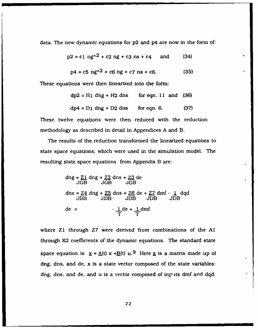
data. The new dynamic equations for p2 and p4 are now in the form of:
p2 = cl ngA2 + c2 ng + c3 ns + c4 and (34)
p4 = c5 ngA2 + c6 ng+ c7 ns + c8. (35)
These equations were then linearized into the form:
dp2 = Hi dng + H2 dns for eqn. 11 and (36)
dp4 = Di dng + D2 dns for eqn. 6. (37)
These twelve equations were then reduced with the reduction
methodology as described in detail in Appendices A and B.
The results of the reduction transformed the linearized equations to
state space equations, which were used in the simulation model. The
resulting state space equations from Appendix B are:
dng = Z1 dng + Z2 dns + Z3 deJGB JGB JGB
dns = Z4 dng + M dns + a de + Z7 dmf - L dqdJDB JDB JDB JDB JDB
de = - lde + 1 dmfT T
where ZI through Z7 were derived from combinations of the Al
through K2 coefficients of the dynamic equations. The standard state
space equation is x = A(t) x +B(t) u. 9 Here X is a matrix made up of
dng, dns, and de, x is a state vector composed of the state variables:
dng, dns, and de, and u is a vector composed of inp'its dmf and dqd.
22

The A and B matrices are:
All = Z A12 = Z2 A13 = Z3
JGB JGB JGB
A21 = Z4 A22 = Z5 A23 = ZJDB JDB JDB
A31 = O A32 = O A33 = -1
T
and Bil =O B12 =O
B21 = Z7 B22= -1JDB JDB
B31 = -1 B32 = OT
and the state space equations now appear as:
dng = A11 dng + A12 dns + A13 de + B 11 dmf + B12 dmf
dns = A21 dng + A22 dns + A23 de + B21 dmf + B22 dmf
de = A31 dng + A32 dns + A33 de + B31 dmf + B32 dmf.
A coarse tuning was next performed to determine the best
numerical values of the coefficients. This was necessary since the first
set of regressed coefficients did not provide accurate simulation. This
was attributed to the coarse instrumentation that is present on the
NPS turbine and the manner of fitting in the regression routine.
Consequently, attention was focused on the following coefficients as in
need of tuning: Al, A2, B1, B2, Cl, C2, Fl, and 11 - 15. Those for D1.
D2. Hl, H2, Kl, and K2 were found previously using the data
23

regression program. Initially chosen for a starting point was that for
B2 (ma/ap2). This was an obvious choice for much is known about
the relationship between ma and p2 in compressors. To find B2, p2
was plotted versus ma at constant ng values. From this the slope
ama/ap2 (B2) was obtained. The B1 expression (ama/ang) was found
by regression using the plotted value of B2 in the Minitab routine. A2
and C2 were then found using plotted values to find the slopes at2/ap2
(A2) and qc/ap2 (C2). These were then used as inputs into the
relationships:
B1 = ama/ang = Al = at21ang = -C1 =age/LngB2 ama/ap2 A2 at2/p2 C2 aqc/Dp2
from which Al and Cl were obtained. The results were then checked
and verified through the use of the data regression program. At steady
state qc = qhpt is required, thus the relationship for CI (dqc/Dng) = 14
(aqhpt/ang). So, with 14 determined, the value of 11 (aqhpt/ama) can
be found as 11 = 14/B1 and 12 (Dqhpt/at2) is 14/Al. With these three,
11, 12, and 14, as inputs, 13 (aqhpt/ap4) and 15 (Wqhpt/amf) were
obtained through the use of the data regression routine. The
numerical values can be found in Appendix C.
The next step involves fine tuning the computer simulation model
and results in the setting of the remaining coefficients of the A and B
matrices.
24

IV, FIOE TUNING THE MODEL
In fine tuning, the actual dynamic data was used in conjunction with
a simulation approach to select final values for the model constants.
The simulation approach used the simple linear state space
equations for dng, dns, and de. These described a first order
differential equation set, -with time varying A and B matrices, to mimic
the actual nonlinearity of the system response. This was accomplished
by approximating the true nonlinear relationships with a series of
small linear steps as depicted in figure 7.
The dynamic simulation computer model was developed from a
routine written by Herda and later modified by Stammetti, it is shown
in figure 8. The major change to the previous program was in the A
and B matrix equations. In the past, the equations were complex
and were a combination of exponentials and second order equations.
In the present model they were simple, first order linear functions of
the states. Another change which occurred in the fine tuning process
was the adjusting of the dynomometer shaft inertia. This change
was for shaping the response and did not affect the steady state
response of the model.
A. Computer Simulation
The simulation program was built using four sections. These were
25

State
Sequential
Actual Reponse
Time
Figure 7. Sequential Linearization.
Input: -b u
A(t), B(t)
Compute: x = A(t) x +. B(t) u
L- f x dt
Figure 8. Simulation Process.
26

the dynamic data input, the initial condition, the dynamic, and the
derivative sections. The actual dynamic data was taken on a four
channel strip chart recorder and depicts the real turbine response of
Ng, Ns, Qd, and Mf as a function of time. These dynamic runs were
compiled in Appendix E and provided the source and data for the
simulation. The initial condition section established the initial
conditions for each particular run. The dynamic section formulated
the display of the dynamic data and was followed by the derivative
section which formulated the simulated response. The outputs of
these final two sections were then plotted for comparison. These
plotted results were used to assist in a grid search on the still doubtful
component coefficients to determine the final values of the A and B
matrices. The procedure was to guess values of the coefficients, then
simulate the model response. If the model and the data agreed, then
the search was over.
B. The Grid Search
A grid search technique was applied in two and three parameter
searches to find the optimal values for the remaining coefficients. It
was formed using a the spread sheet formatted program called Excell,
by Microsoft software. An example of this is found in Appendix C. The
top portion provided the inputs for the coefficients used in the
calculation of the A and B matrices. The middle portion calculated the
27
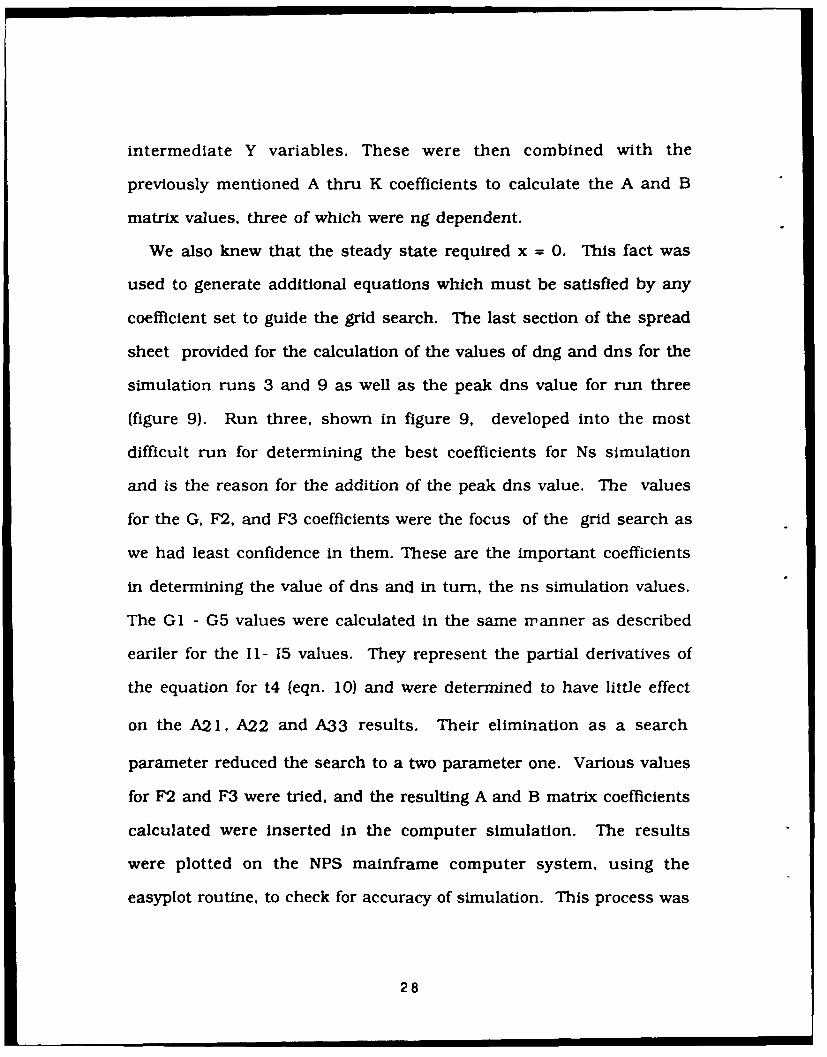
intermediate Y variables. These were then combined with the
previously mentioned A thru K coefficients to calculate the A and B
matrix values, three of which were ng dependent.
We also knew that the steady state required x = 0. This fact was
used to generate additional equations which must be satisfied by any
coefficient set to guide the grid search. The last section of the spread
sheet provided for the calculation of the values of dng and dns for the
simulation runs 3 and 9 as well as the peak dns value for run three
(figure 9). Run three, shown in figure 9, developed into the most
difficult run for determining the best coefficients for Ns simulation
and is the reason for the addition of the peak dns value. The values
for the G, F2, and F3 coefficients were the focus of the grid search as
we had least confidence in them. These are the important coefficients
in determining the value of dns and in turn, the ns simulation values.
The GI - G5 values were calculated in the same nmanner as described
eariler for the 11- 15 values. They represent the partial derivatives of
the equation for t4 (eqn. 10) and were determined to have little effect
on the A21, A22 and A33 results. Their elimination as a search
parameter reduced the search to a two parameter one. Various values
for F2 and F3 were tried, and the resulting A and B matrix coefficients
calculated were inserted in the computer simulation. The results
were plotted on the NPS mainframe computer system, using the
easyplot routine, to check for accuracy of simulation. This process was
28

32000 X X
RUN 9
29000
NG
26000 RUN 3 RUN 7
(RPM)
23000
RUN 1
20000 X X
I I 1 I - -
500 1000 1500 2000 2500
Ns (RPM)
Figure 9. Dynamic Data Runs.
repeated until the optimal F2 and F3 values were obtained.
29

V. VALIDATION OF THE MODEL
The validation of the model was a two step process which carried
over from the fine tuning. After the fine tuning was complete, and
the model resulted in the proper shape for runs 3 and 9. and with the
steady state response within the required tolerances, the first step
was complete. The next step was to take the model and apply it
elsewhere in the operating range of the turbine to check for accuracy.
If the proper response in shape and prescribed tolerance criteria (+/
- 10 percent in the dynamic and steady response) were still met,
then the validation was completed. This process was only performed
around the borders of the operating range (figure 9). If successful,
then the model should be applicable anywhere in the turbine
operating range.
The first run modeled was the one for run nine which models the
Ns transient response from 500 to 2500 rpms while holding the value
for Ng, as load varies, constant at 32000 rpms (+/- 5%) for the
conditions shown in run nine in Appendix E.. Figure 10 is the
graphical representation of the modeled run and the dynamic data run
for this transient. The criteria has been met for run 9, so the model
was applied to the validation run one. Run one, simulates the
transient for Ns from 500 to 2215 rpms (the turbine will not operate
above 2215 rpm at low Ng) with the value for Ng constant at 20000
30

SIMULATION RUN 9 NG
LEGENDr DATA
SIMULATION
10 20 30 40 so
TIME (SEC)
SIMULATION RUN 9 NS
0/
LEGENDo DATA
00 SIMULATION
6 10 20 30 40 50
TIME (SECi
Figure 10. Simulation-Run Nine.
31

VALIDATION RUN I NG
0
LEGENDDATASIMULATION
10 20 30 40 50TIME (SEC)
VALIDATION RUN I NS
0 0
zo
C I.ma
LEGENDa DATA
SI MULATION
10 io 30 4o0sTIME (SEC)
Figure 1 1. Validation-Run One.
32

rpms (+/- 5%); the results are shown in figure 11. Again, the
accuracy criteria were met. This covers the upper and lower bounds
of the operating range.
Next, run three was used in conjunction with run nine in the fine
tuning portion. This run is a vertical run on the left side of the
operating range and is an Ng transient from 20000 to 32000 rpms
with Ns being held constant at 500 rpms to conform with the actual
dynamic data run. This run is shown in figure 12. Note that the
accuracy criteria are easily met in Ng but apparently not satisfied in
Ns. However, when the accuracy criteria is applied to the normalized
Ns, the transient is acceptable. To validate this run the model is next
applied to the right hand side of the operating range. This is run
seven and, again, is a Ng transient from 20000 to 32000 rpms with Ns
slightly increasing from the lower constraint of 2215 rpm to 2500
rpms which is attainable at the upper limits of the operating range.
This run is presented in figure 13. A validation run was attempted
vertically in the center of the operating range. This is run five and
it's response was of the same result shown in figure 11 for run seven
and therefore was not shown as a separate figure.
33

SIMULATION RUN 3 NG
LEGEND
oDATASIMULATION
1 0 20 3'0 40 50
TIME (SEC)
SIMULATION RUN 3 NS
Za
LEGENDoDATA
0 10 iO 40 50TlIME (SEC)
Figure 12. Simulation-Run Three.
34
I I I

VALIDATION RUN 7 NG
0
C
z 0
0
ej ------ -- -- -to152
TIE(SC
AIATORU77N
0 tois2
TIM (SCFiur 3.VaiatonRn evn
35
a LEGEN

VI. CONCLUSIONS
A modeling method has been developed for real time simulation of a
marine gas turbine. The results of this modeling method should be
used with the LQR controller design theory to develop a new
controller for the Boeing test bed at NPS. This controller should then
be tested to ascertain it's abillLy to be more fuel efficient than the
present system.
This model was simple in that it used matrix elements for A and B
which were only linear state functions. The dependency was only on
the Ng state. This simplicity will provide fast run times on a small
computer for model reference control and diagnostics.
Accurate simulation performance has been demonstrated in the
compressor/high pressure turbine section and the resulting steady
states have been achieved to +/- 3%. An exception to this accuracy is
the constant Ns simulation for the vertical runs . This is only an
indication that the final values for F2, F3, and possibly GI are not fine
tuned enough to provide for more accurate constant Ns response.
Investigation was conducted into this irregularity to determine the
cause of the steady state results being to high. The fact that the steady
state response for a constant Ns is higher in runs five and seven was
probed and a number of solutions were looked at. One such solution
was to check for the possibility that the oscillating torque for runs five
36

and seven shown in Appendix E was causing the Ns value to continue
to rise and settle out at a higher steady state. These oscillations do
not appear to be the cause nor have any affect on the steady state
response of Ns. This was verified by modifying the computer
simulation routine so as to remove the oscillation. Another solution
was to adjust the A21 values until a proper steady state value for ne was
reached. At the time of publication this has not provided any
satisfactory results. Another possibility is that the A21 coefficients
may have to change the sign to produce the proper response. The last
area to examine as a possible solution to this problem is to input a
varying inertia for the water brake dynamometer. In the past this
inertia has been assumed to be a constant value when, in fact, it
actually changes with the addition and subtraction of water.
The last recommendations for this project encompass the entire
project. First, a digital data acquisition system should be used to get
the steady state and dynamic data. This will make the fine tuning
process with the data regression program more accurate. Finally, one
computer system should be used for the whole process, from the
regression and grid search to the computer simulation (vice the two
system used in this project). In this way, results could be achieved
and correlated in a more efficient manner.
The model was robust in that, with the exception of the constant
Ns in the vertical runs, the model was applicable to all areas of the
37

operating range. This was supported by the excellent response in Ng
throughout the whole operating range. This shows that the
coefficients for the Al 1, A12, and A13 were accurate and the
procedure to find them was sound.
Once the proper values for A2 1, A22, and A23 are found and this
modeling technique has been successfully demonstrated on the Boeing
engine this method will have real time application to the future
controller design for the General Electric LM- 2500 and the follow on
marine gas turbine controllers designed for the future.
38
.... ~ ~ , , IIII I

APPENhDICES,
APPENDIX A. COMPONENT MODELING EQUATIONS
APPENDIX B: EQUATION SET REDUCTION METHODOLOGY
APPENDIX C: PARAMETER SELECTION METHODOLOGY
APPENDIX D: COMPUTER SIMULATION CODES
APPENDIX E: SOURCE DATA RUNS
39

APPENDEK A
COMPONENT MODELING EQUATIONS:
Compressor
I ma dt2= Al dng +A2 dp2 .......... 1
t2 dma= B Idng + B2 dp2 ............. 2
p2 dqc= C I dng + C2 dp2 ............. 3
Gas Generator Shaft
qc - 4 qhpt JGB dng = dqhpt-dqc ...... 4
ng - g ng
Dynamometer Shaft
qfpt qd JDB dns = dqfpt-dqd ...... 5
ns ns
40

Free Power Turbine
maf - dp4=Didng + D2dns ............ 6
t4
p4 dqfpt = Fl ins+F2 dt4+F3 dmaf ... 7
'O' , qfpt I ns
High Pressure Turbine
Mf
de =(dmf-de)/T ..... 8e
ma - a- maf
t2 t4
p 2 p4
From Continuity:qhpt ng
dmaf = K1 dmf + K2 dma ...... 9
dt4 = G1 dma + G2 dt2 + G3 dp4 + G4 dng + G5 de .................. 10
dp2 = H i dng+ H2 dns .................................................................. 11"
dqhpt=Ildma+ 12dt2 +13dp4 +I4dng +I5de ................... 12
41

Note: 1. Lower case variables represent normalized variables.
2. The d - represents the perturbation of the variable.
" Decoupling equaUons.
42

EQUATION SET REDUCTION METHODOLOGY:
The equations in appendix A are reduced into the statc space
cnoiponents of the A and B matrices.
Substitute eqn 1I:
dp2 = H l dng + H 2 dns .................................................................. 11
into eqns 1, 2, and 3 for dp2.
dt2 = (A1 + A2H1) dng+ {A2H2) dns ................................................. 1
dma = (BI + B2HI} dng + (B2H2) dns ............................................. 2
dqc = (C1 + C2H1) dng + (C2H2) dns ............................................... 3
In eqn 12:
dqhpt = 11 dma + 12 dt2 + 13 dp4 + 14 dng + 15 de .................... 12
substitute eqns 1, 2, and 6 for dt2, dma, and dp4.
dqhpt = 11 (BI + B2H1) dng + 11 (B2H2) dns +
12 (Al + A2HI) dng + 12 (A2H2) dns +
13 (Di) dng + 13 (D2) dns +
14 dng + 15 de ................................. 12
43

Collect terms:
dqhpt = (Ii (Bi + B2H1) + 12 (Al + A2H1) + 13 (D1) + 14 ) dng +
(II (B2H2) + 12 (A2H2) + 13 (D2)) dns + 15 de
Let YlI 11 (B1 +B2H)+12(Al +A2H1)+13 (D1)+1 4
Y2 = II (B2H2) + 12 (A2H2) + 13 (D2)
Then: dqhpt = Yl dng + Y2 dns + 15 de ...................... 12
Take eqn 4 and substitute in new eqn 12 for dqhpt and eqn 3 for
dqc.
JGB dng = YI dng + Y2 dns + 15 de -
(Cl + C2H1) dng - (C2H2) dns
Collect terms:
dng = (CYI - (Cl + C2HIl)) dng + (Y2 - (C2H2)) dns + 15 de )/JGB
Let: Z1 =(YI - (C1 + C2HI)
Z2 = Y2 - (C2H2)
Z3 = 15
Then:
dng = (ZI dng + Z2 dns + Z3 de)/JGB ................ RI
44

In eqn 10:
dt4 = Gi dma + G2 dt2 + G3 dp4 + G4 dng + G5 de ............. 10
substitute eqns 1. 2. and 6 for dt2, dma, and dp4.
dt4 = G1 (Bi + B2H1) dng + Gi (B2H2) dns +
G2 (Al + A2HI) dng + G2 (A2H2) dns +
G3 (D1) dng + G3 (D2) dns +
G4 dng + G5 de ................................. 10
Collect terms:
dt4 = (Gi (BI + B2H1) + G2 (Al + A2H1) + G3 (DI) + G4) dng +
(Gi (B2H2) + G2 (A2H2) + G3 (D2) ) dns + G5 de
Let Y3= "1 (B1 +B2H1) +G2 (Al +A211) + G3 (DI) + G4
Y4 = G1 (B2H2) + G2 (A2H2) + G3 (D2)
Then: dt4 = Y3 dng + Y4 dns + G5 de ....................... 10
In the continuity eqn (9) substitute eqn 2 for dma.
dmaf= Ki dmf+ K2(Bi + B2Hl) dng + K2(B2H2) dns .......... 9
Substitute new eqn 10 for dt4 and new eqn 9 for dmaf into:
eqn 7: dqfpt =F1 dns + F2 dt4 + F3 dmaf
This results in:
45

dqfpt = F1 dns + F2Y3 dng + F2Y4 dns + F2G5 de +
F3Kl dmf + F3K2(Bl + B2Hl) dng + F3KQ(B2H2) dns
Collect terms:
dqfpt = (F2Y3 + F3K2(Bl + B2H 1)) dng +
(F1 + F3K2(B2H2) + F2Y4) dns + F2G5 de + F3K1 dmf
Let: 14 = FO2Y3 + F3K2 (B I + B2H 1)
Z5 =Fl + F3K2(B2H2) + F2Y4
Z6 =F2G.5
Z7 = F3Kl
Then:
dqfpt =Z4 dng +Z5dns +Z6 de +Z7dmf ........ 7
Substitute new eqn 7 for qfpt in eqn 5.
JDB dns =dqfpt -dqd...... .............................. 5
dns =(Z4 dng +Z5 dns +Z6 de +Z7 dmf- dqd)/JDB ............ R2
Finally: Eqn, 8 is R3. Ri. R2, and R3 make up the state space
equation set.
46

The state space equation set is the following:
dng = Zl dng + M dns + Z de .................... R1JGB JGB JGB
dns = Z4 dng + Z5 dns + Z& de + Z7 dmf - 1 dqd ..... R2JDB JDB JDB JDB JDB
de = -.. Lde + .idmf ................... RT T
The resulting A and B matrices are:
All =Zl Ai2 = Z2 A13 = Z3JGB JGB JGB
A21 = Z4 A22 = Z5 A23 = Z6JDB JDB JDB
A31 = O A32 = O A33= -1T
andBi =O B12=O
B21 = Z7 B22 = -1
JDB JDB
B31= 1 B32 = OT
47

PARAMETER SELECTION METHODOLOGY:
The parameter selections were accomplished through three means:
1. Plotting actual slopes from data. This was shown
in chapter III section F.
2. Data reduction using mainframe program
Mini-Tab.
3. Grid searching using coefficients from 1. and 2.
and known relationships which must be satisfied.
The spread sheet is from the Micro-soft program
Excell and was used on an Apple Macintosh
computer.
The data reduction program Minitab was used for all of the
regressions performed. The input for the regression program was the
steady state turbine data shown in table 1 A. This routine was used to
determine the order of the independent variables in the equations for
Ma, T2, and Qc, as well as to regress the expressions for P2, P4, T4,
Qhpt and Maf. To determine the order of a independent variable a
three step process was followed. First, the dependent variable was
regressed using the data for the independent variables. In doing this a
residual was calculated for each set of the independent variables. This
was then subtracted from the regressed value of the dependent
48

variable. The resulting difference was plotted versus each of the
independent variables. In the plot for the regression of T2, shown in
figure C-la, there is a definite parabolic shape which is an indication
that the independent variable in question (Ng) is of a higher order. To
verify this, T2 was regressed again, this time using NgA2 , Ng and P2.
The plotting was repeated with the resultant plot shown in figure C-
lb. This time the parabolic shape was not in evidence and the
predictor percentage, which indicates the accuracy of the regression
based on the data, increased from 99.6 to 99.9 percent indicating an
excellent regression for the t2 equation. The resulting partials for all
of the component expressions are shown in figure C-2 lines 3 through
21.
The spreadsheet grid, figure C-2, was used in conjunction with the
simulation program to search out the best values for the rest of the
coefficients in the equations in appendix A. These were input for G1,
F2, and F3 in lines 3-21 and then used in lines 25-32 to calculate the
values of the coefficients of the A and B matrices. Lines 34-38 show
the proper signs for these matrix coefficients as well as the dns and
dng relationships which must be satisfied during the search process.
Once these were satisfied, plots were generated and checked for the
accuracy of the simulation.
49

--N
3.5+ 3-
- N
T2- -0.0+
residual -
-3.5+ -N
2
20000 22500 25000 27500 30000 32500
Ng
(A)
T2 - 2.0+
residual - NN N
0.0+ 2 N- 2 N2
-N
-2.0+
------------------------------------ +----------------------
20000 22500 25000 27500 30000 32500
Ng
(B)
Figure C-1. Regression Plots
50

A B C D E F 0
4 A AX NO B X NO C C X NO5 1 -2.6 13.15 -1.06 5.36 -2.415 12.216 2 -3.5 -1.427 -3.25
9 D_____ D_____ X_____ NO____ F X NO K
1010___,___ 1 -1.97 4.36 -0.06 -0.445 0.0141I 1 2 0.039 -1.55 0.97512 3 2.5131141151161 0 OX NO H HX NO I I XNOI17 1 0.020335 - 1.44 3.62 2.27818 2 0.00829111 0.0134 0,928819 3 -00925698 - 103720 4 -0.021558 0,10899489 -2.415 12.2121 5 0.12161723 13.624_222324 y Y XNO Z Z XNo25, 1 22.5465086 -32.114852 20.28150861 -32.559852 A 1126, 2 -0.4915502 -0.4480002 A1I22"7 3 0.20 126569 -0.2866793 13.624 A1328 4 -0,0043879 2.113058171 0.91786171 A2129 5 -0.0998081 -0.445 A2230 6 RUN 3 ,nog 1.23769231 -0,1885067 A2331 7 RUN 9 no= 1,23653846 0.03525 B2132 PEAK no = 1.2363076933,34 RUN 3 A g= -0.0001131 dis = 0,00094893 -All -A12 +A1335-- - - - -- - - - -36 RUN 9 dl'g = 0.25454755 dds = -0.0113783 + A21 -A22 + A2337 - - - - - - - - -38 PEAK drs - 1O. 127,69172 0 0 -A33391401
Figure C-2. Sample Grid Search Spread Sheet.
51
13. __ _ _ _ __ __ __ _ __ ___l__ __ _

APMIINDX 12
COMPUTER SIMULATION CODES:
The computer codes were written using the Dynamic Simulation
Language (DSL).
Simulation Run 1: DSL code for dynamic Ns run at constant Ng
(20000 rpm).
Simulation Run 3: DSL code for dynamic Ng run at constant Ns
(500 rpm).
Simulation Run 5: DSL code for dynamic Ng run at constant Ns
(1500 rpm).
Simulation Run 7: DSL code for dynamic Ng run at Ns
( 2252-2500 rpm).
Simulation Run 9: DSL code for dynamic Ns run at constant Ng
(32000 rpm).
52
lt H ii ing f i IWW"

* BOEING MODEL 502-6A GAS TURBINE *
* DYNAMIC COMPUTER SIMULATION *
* MODIFIED BY ** S.D. METZ ** FROM ROUTINES BY ** V.J. HERDA AND V.A. STAMMETTI *
* THIS PROGRAM SIMULATES THE DYNAMIC RESPONSE OF THE NPS ** BOEING GAS TURBINE TEST FACILITY USING A MULTILPLE ** LINEARIZATION TECHNIQUE. *
CC
PARAM JG=0.009525, JD=0.3000, PI=3. 14159, TC=1.0
* THE FOLLOWING VALUES LISTED ON THE FUNCTION CARD ARE FOR FUEL FLOW,* GAS GENERATOR SPEED, TORQUE AND DYNO SPEED AS A FUNCTION OF TIME.* THESE VALUES WERE OBTAINED FROM STRIP CHART RECORDS AND ARE ENTERED
* IN THE FORM (E.G. FUEL FLOW) ... TIME(SEC), FUEL FLOW .....
CC THIS SET IS FOR EXPERIMENTAL RUN # 1.CCAFGEN NGDATA= 0.0,20230.0, 5.0,20230.0, 10.0,20230.0, 15.0,20230.0,
20.0,20230.0, 25.0,20230.0, 50.0,20230.0AFGEN NSDATA= 0.0,505.0, 1.0,505.0, 2.0,536.7, 3.0,568.33,
4.0,600.0, 5.0,631.7, 6.0,695.0, 7.0,790.0, 8.0,885.0,9.0,1043.3, 10.0,1170.0, 11.0,1328.3, 12.0,1486.7,13.0,1708.3, 14.0,1835.0, 15.0,1930.0, 16.0,1993.3,17.0,2056.7, 18.0,2088.3, 19.0,2120.0, 20.0,2151.7,21.0,2167.5, 22.0,2177.0, 23.0,2183.3, 24.0,2215.0,25.0,2215.0, 50.0,2215.0
AFGEN MFDATA= 0.0,78.39, 5.0,78.39, 10.0,78.39, 12.0,79.89,15.0,80.26, 17.0,80.26, 19.0,81.38, 20.0,82.50,21. 0,82. 13, 25. 0,82. 13, 50.0,82.13
AFGEN QDDATA= 0.0,125.0, 1.0,125.0, 2.0,118.3, 3.0,115.0,4.0,111.7, 5.0,105.0, 6.0,98.33, 7.0,85.0, ...8.0,71.67, 9.0,58.33, 10.0,45.0, 11.0,31.67,12.0,11.67, 12.5,1.670, 13.0,5.0, 15.0,5.0,25.0,5.0, 50.0,5.0
INITIAL* ESTABLISH INITIAL CONDITIONS.
NGI=20230. 0NSI=505 0MFI = 78. 39QDI = 125. 0
* SET INITIAL STATE PERTURBATION TO ZERO
DNG = 0.0DNS = 0. 0DE = 0.0
53

NGB = 26000.0NSB = 1500.0MEB =122.5QDB = 220.0QCB = 80.0JGB = (NOB/QCB)*JG3DB =(NSB/QDB)*JD
DYNAMIC
* DATA CURVE FORMULATION
NOD =AFGEN(NODATA,TIME)NSD =AEOEN(NSDATA,TIME)MFD =AFOEN(MFDATA,TIME)QDD =AFOEN(QDDATA,TIME)
MEDLY -TRANSP(100,MFI,0.70,MFD)
* STATE SPACE LINEAR MODEL FORMULATION
All =(20. 282-32. 560*(NGL/NGB))/( JOB)
A12 -(-0.4480)/(JGB)
A13 =(13. 624)/( 3GB)
A21 =(2. 1131+.91786*(NGL/NGB))/(JDB)
A22 =(-.0998-0.445*(NGL/NCB))/(JDB)
A23 =(-0.1885)/(JDB)
A31 =0.0
A32 = 0.0
A33 = -1. 0,'TC
B11 = 0.0
B12 = 0.0
B21 =.035250/(JDB)
B22 = -1. 0/( DB)
B31 = .0/TC
B32 = 0.0
DERIVATIVENOSORT
* COMPUTE INPUT TO THE NONLINEAR MODEL, MF(T), WW(T).* RUN #9
DMF =(MFDLY - MFI)/MFBDQD =(QDD - QD)I)/QDBDHGOOT =A11*DNG + A12*DNS +A13*DE + B11*DMFDNSDOT =A21*DNG + A22'4DNS +A23*DE + B21*DME + B22*DQD
DEDOT =A33*DE * B31*DMF
* DYNAMIC EQUATIONS FOR LINEAR MODEL.DNCG'INTGRL(0. 0,DNGDOT)DNS=INTGRL(0. 0,D)NSDOT)DE =INTGRL(.0. ,DEDOT)NGL NSI + DNC *NGBNSL =NSI + DNS*ISB
SORT
54

* THE STATEMENTS IN THE PREVIOUS (DERIVATIVE) SECTION YIELD VALUES* OF 'NO', AND 'NS' AS CALCULATED BY THE NONLINEAR AND STATE SPACE' MODELS. THE STATEMENTS BELOW COMPUTE THE VALUES OF 'NG', AND 'NS'* AS RECORDED FROM GAS TURBINE TEST DATA.
TERMINALMETHOD RKSCONTROL FINTIM=50. O,DELT=O. 001PRINT 0.5,NGD,NGLNSD,NSL,MFD,QDDENDSTOP
55

* BOEING MODEL 502-6A GAS TURBINE *
* DYNAMIC COMPUTER SIMULATION
* MODIFIED BY* S.D. METZ *
FROM ROUTINES BY ** V.J.HERDA AND V.A. STAMMETTI
* THIS PROGRAM SIMULATES THE DYNAMIC RESPONSE OF THE NPS *
* BOEING GAS TURBINE TEST FACILITY USING A MULTILPLE ** LINEARIZATION TECHNIQUE. *
CCPARAM JG=O.009525, JD=O.3000, PI=3. 14159, TC=1.OO
* THE FOLLOWING VALUES LISTED ON THE FUNCTION CARD ARE FOR FUEL FLOW,
* GAS GENERATOR SPEED, TORQUE AND DYNO SPEED AS A FUNCTION OF TIME.* THESE VALUES WERE OBTAINED FROM STRIP CHART RECORDS AND ARE ENTERED* IN THE FORM (E.G. FUEL FLOW) ... TIME(SEC), FUEL FLOW .....
CC THIS SET IS FOR EXPERIMENTAL RUN # 3.CCAFGEN NGDATA= 0.0,20220.0, 3.55,20220.0, 3.7,20315.7, 3.8,20411.4,
4.0,20698.4, 5.0,23186.1, 6.0,25482.4, 7.0,27204.6,8.0,28926.9, 9.0,30649.1, 10.0,32180.0, 10.5,32371.4,11.0,32180.0, 11.5,32084.3, 12.0,32180.0, 50.0,32180.0
AFGEN NSDATA= 0.0,506.0, 2.0,505.7, 3.6,505.5, 4.0,506.5, ...5.0,508.3, 6.0,509.7, 7.0,511.1, 8.0,512.5, 9.0,513.5,10.0,514.4, 10.4,514.7, 11.0,514.4, 12.0,515.1,13.0,515.8, 14.0,516.7, 16.3,517.2, 27.0,526.7,18.0,515.8, 19.0,514.9, 20.0,513.0, 50.0,513.0
AFGEN MFDATA= 0.0,77.5, 3.0,77.5, 3.3,79.6, 3.6,85.8, ...4.0,91.99, 5.0,106.5, 6.0,118.9, 7.0,130.5, 8.0,241.3,9.0,156.2, 10.0,172.7, 11.0,156.2, 12.0,160.3, 50.0,160.3
AFGEN QDDATA= 0.0,125.0, 3.6,125.O, 3.8,128.4, 4.0,131.8, ...5.0,172.4, 6.0,226.7, 7.0,274.1, 8.0,321.6, 9.0,375.8,10.0,430.0, 10.5,443.6, 11.0,430.0, 12.0,416.4, ...13.0,416.4, 14.0,419.8, 15.0,416.4, 18.0,423.0, ...20.0,430.0, 50.0,430
INITIALESTABLISH INITIAL CONDITIONS.
NGI=20220.0NSI=506. OMFI = 77.5QDI = 125.0
* SET INITIAL STATE PERTURBATION TO ZERO
DUG = 0.0DNS = 0-0DE = 0.0
56

NOB = 26000.0NSB = 1500.0MFB = 122.5QDB = 220.0QCB = 80.0JGB = (NGB/QCB)*JOJDB = (NSB/QDB)*JD
DYNAMIC
* DATA CURVE FORMULAT ION
NOD = AFOEN(NGDATA,TIME)NSD = AEGEN(NSDATA,TIME)MFD = AFGEN(MFDATA,TIME)QDD = AFGEN(QDDATA,TIME)
MFDLY = TRANSP(100,MFI,0.70,MFD)
* STATE SPACE LINEAR MODEL FORMULATION
All =(20. 282-32. 560*( NOL/NGB) )/( JOB)
A12 =(-0. 448)/(JGB)
A13 = ( 13. 62 4)/( JGB)
A21 = (2. 1131+.91786*(NGL/NGB))/(JDB)
A22 = (-.0998-O.445(NGL/NGB))/(JDB)
A23 =(-. 18851)/(JDB)
A3 .
A32 = 0.0
B32 = 0. 0
B22 = -1.0/TCDB
B31 = 0.0/T
B32 = 0.0
B22 =(FL -O,'(JDB)
B31 =(D -.O/TQD
DERO = lIVE+B1*M
DYCOMPUTEQINUTIN TOR H LINEAR MODEL FT.W(
DMF (MFDRLYO - MI)/MFBCT
DGNGDOT + AIDG +A2*NS+ I 4 D +BI*
DS NT + A2DS* 22DsNs2BE 2 4 DF+B*QDESORAT3D 31M
*5

* THE STATEMENTS IN THE PREVIOUS (DERIVATIVE) SECTION YIELD VALUES* OF 'NG', AND 'NS' AS CALCULATED BY THE NONLINEAR AND STATE SPACE* MODELS. THE STATEMENTS BELOW COMPUTE THE VALUES OF 'NG', AND 'NS'* AS RECORDED FROM GAS TURBINE TEST DATA.
TERMINALMETHOD RKSCONTROL FINTIM=50. O,DELT=O. 001PRINT 0.50,NGD,NGL,NSD,NSL,MFD,QDD,DNSDOTA21,DNG,
A22,DNS,A23,DE,B21,DMF, B22,DQDENDSTOP
58

* BOE!NG MODEL 502-6A GAS TURBINE *
* DYNAMIC COMPUTER SIMULATION *
* MODIFIED RY ** S.D. METZ ** FROM ROUTINES BY ** V.J.HERDA AND V.A. STAMMETTI *
* THIS PROGRAM SIMULATES THE DYNAMIC RESPONSE OF THE NPS* BOEING GAS TURBINE TEST FACILITY USING A MULTILPLE ** LINEARIZATION TECHNIQUE. *
CC
PAR'%M JG=0.009525, JD=0.3000, PI=3.14159, TC=1.OO
* THE FOLLOWING VALUES LISTED ON THE FUNCTION CARD ARE FOR FUEL FLOW,* GAS GENERATOR SPEED, TORQUE AND DYNO SPEED AS A FUNCTION OF TIME.* THESE VALUES WERE OBTAINED FROM STRIP CHART RECORDS AND ARE ENTERED* IN THE FORM (E.G. FUEL FLOW) ... TIME(SEC), FUEL FLOW .....
C
C THIS SET IS FOR EXPERIMENTAL RUN # 5.CCAFGEN NGDATA= 0.0,20220.0, 3.1,20220.0, 3.6,20412.1, 4.0,21372.6,
5.0,23677.7, 6.0,25886.9, 7.0,27711.8, 8.0,29440.6, ...9.0,30977.4, 10.0,32206.8, 10.2,32322.1, 10.8,32130.0,11.5,32130.0, 12.1,32014.7, 13.4,32206.8, 14.5,32014.7,15.6,32206.8, 16.8,32014.7, 17.0,32206.8, 50.0,32130.0
AFGEN NSDATA= 0.0,1491.6, 1.0,1490.4, 3.0,1489.6, 4.0,1492.5,5.0,1501.0, 6.0,1508.3, 7.0, 1511.7, 7.8,1513.3, ...9.6,1513.3, 10.1,1513.8, 12.0,1508.3, 13.0,1510,0,50.0,1510.0
*
AFGEN MFDATA= 0.0,83.75, 3.2,83.75, 5.0,109.6, 6.0,122.2,7.0,135.5, 8.0,150.2, 9.0,162.8, 9.8,172.4,10.0,168.7, 11.0,165.0, 50.0,165.0
AFGEN QDDATA= 0.0,71.0, 4.4,71.0, 5.0,78.7, 6.0,94. 1,7.0,107.5, 8.0,120.9, 9.0,134.4, 10.2,149.8, .10.9,147.9, 11.6,147.9, 12.4,143.2, 13.0,145.9,13.5,144.0, 14.0,145.9, 15.0,144.0, 50.0,144.0
INITIALESTABLISH INITIAL CONDITIONS.
NGI=20220.0NSI=1491.6MFI = 83.75QDI = 71.0
* SET INITIAL STATE PERTURBATION TO ZERO
DNG = 0. 0DNS = 0. 0DE = 0.0
59

NOB = 26000.0NSB = 1500.0MFB =122.5QDB = 220.0QCB = 80.0JGB = (NGB/QCB)*JGJDB = (NSBIQDB)-JD
DYNAMIC
*DATA CURVE FORM4ULATION
NG FE(NDTIE
NGD = AFGEN(NODATATIME)
MED = AFGEN(MEDATA,TIME)QDD =AFGEN(QDDATA,TIME)
?4FDLY = TRANSP(.100,MFI,0.70,MFD)
* STATE SPACE LINEAR MODEL FORMULATION
All -(20. 282-32. 560*( NOL/NGB) )/( JOB)
A12 = (-O.4480)/(JGB)
A13 = ( 13. 62 4) /( JOB)
A21 = (2. 1131+. 91786*(NGL/NGB))/(JDB)
A22 = (-.0998-0.445*(NGL/NGB))/(JDB)
A23 =(-O. 18851)/C JDB)
A3 .
A32 = 0.0
A33 = 01.0/T
A33 = 0.0/T
B12 = 0.0
B21 =.035250/(JDB)
B22 = -1. 0/(JDB)
B31 = 1.0/TC
B32 = 0.0
DERIVATIVENOSORT
* COMPUTE INPUT TO THE NONLINEAR MODEL, MF(T), WW(T).* RUN #9
DMF =(MFDLY - MFI)/MEBDQD =(QDD - QDI)IQDBDN4GDOT =AI1*DN0 + A12*DNS + A13*DE + B1I*D?,IFDNSDOT = A21*DNG + A22*DNS + A23*DE + B21*DMF + B22*DQDDED0T =A33*DE + B31*DMF
* DYNAMIC EQUATIONS FOP LINEAR MODEL.DNC I NTGRL( 0 0, ONGDOT)DNS=I NTGR L( 0. 0,DNSDOT)DE =ZNTC'iO.OI7ED0T)NGL -11' + D11r1CflO!ISL =NSI + N 4 IS
C~. r)-
60

* THE STATEMENTS IN THE PREVIOUS (DERIVATIVE) SECTION YIELD VALUES* OF 'NG', AND 'NS' AS CALCULATED BY THE NONLINEAR AND STATE SPACE
SMODELS. THE STATEMENTS BELOW COMPUTE THE VALUES OF 'NG', AND 'NS'* AS RECORDED FROM GAS TURBINE TEST DATA.*
TERMINALMETHOD RK5CONTROL FINTIM=50.O,DELT=0.001PRINT 0.5,NGD,NGL,NSD,NSL,MFDQDD,DNSDOT.A21,DNG,A22,DNS,
A23,DE,B21,DMF,B22,DQDENDSTOP
61
61

| *
* BOEING MODEL 502-6A GAS TURBINE *
* DYNAMIC COMPUTER SIMULATION *
* MODIFIED BY *
* S.D. METZ a* FROM ROUTINES BY ** V.J. HERDA AND V.A. STAMMETTI *
* THIS PROGRAM SIMULATES THE DYNAMIC RESPONSE OF THE NPS ** BOEING GAS TURBINE TEST FACILITY USING A MULTILPLE ** LINEARIZATION TECHNIQUE. *
CCPARAM JG=0.009525, JD=0.3000, PI=3.14159, TC=1.00
* THE FOLLOWING VALUES LISTED ON THE FUNCTION CARD ARE FOR FUEL FLOW,* GAS GENERATOR SPEED, TORQUE AND DYNO SPEED AS A FUNCTION OF TIME.* THESE VALUES WERE OBTAINED FROM STRIP CHART RECORDS AND ARE ENTERED* IN THE FORM (E.G. FUEL FLOW) ... TIME(SEC), FUEL FLOW .....
CC THIS SET IS FOR EXPERIMENTAL RUN # 7.CCAFGEN NGDATA= 0.0,20220.0, 4.0,20220.0, 4.5,20759.7, 5.0,21954. 7,
6.0,24460.3, 7.0,26541.9, 8.0,28122.4, 9.0,29780.0,10.0,31399.0, 10.4,32092.9, 10.6,32362.7, 11.0,32285.6,12.0,32170.0, 15.0,32170.0, 20.0,32170
AFGEN NSDATA= 0.0,2252.0, 1.0,2245.4, 2.0,2238.8, 3.0,2232.2,4.0,2225.6, 5.0,2278.4, 6.0,2436.8, 7.0,2568.8,7.7,2621.6, 8.0,2611.0, 9.0,2579.4, 10.0,2568.8, .11.0,2542.4, 13.0,2516.0, 15.0,2516.0, 20.0,2516
AFGEN MFDATA= 0.0,78.8, 1.0,78.8, 3.0,78.8, 4.0,87.1 ...4.5,95.3, 5.0,103.6, 6.0,111.9, 7.0,128.5, 8.0,136.8,9.0,161.7, 10.0,174.1, 10.4,178.3, 11.0,170.0,15.0,170.0, 20.0,170.0
AFGEN QDDATA= 0.0,25.0, 2.0,25.0, 4.0,25.0, 5.0,25.0,6.0,49.6, 7.0,92.6, 8.0,129.4, 9.0,178.6, ...10.0.33.9, 11.0,264.6, 12.0,252.3, 13.0,246.1,15.0,240.0, 20.0,240.0
INITIAL
* ESTABLISH INITIAL CONDITIONS.
NGI=20220. 0NSI=2252.0MFI = 78.75QDI = 25.0
* SET INITIAL STATE PERTURBATION TO ZERO
DNG = O. 0DNS = 0. 0DE = 0.0
62

NGB = 26000.0NSB = 1500.0t4FB = 122.5QDB = 220.0QCB = 80. 0JGB = (NGB/QCB)*JGJDB = (NSB/QDB)*JD
DYNAMIC
*DATA CURVE FORMULATION
NG EE(NDTIE
NSD = AFGEN(NSDATATIME)NSD = AFGEN(NSDATATIME)
QDD = AFGEN(QDDATATIME)MFDLY = TRANSP(l00,MFI,O.70,MFD)
* STATE SPACE LINEAR MODEL FORMULI.ATION
All = (20.282-32. 560*(NGL/NGB) )/( JOB)
A12 = (-0. 448)/( JGB)
A13 =(13. 624)/( JOB)
A21 = (2. 1131+. 91786*(NGL/NOB))/(JDB)
A22 = (-.0998-0. 4454 (NGL/NGB))/(JDB)
A23 = (-. 28851)/(JDB)
A3 .
A32 = 0.0
B12 = 0.0
B22 = -1.0/ICDB
B31 = 0.0/T
B32 = 0.0
DERVAIV
D22 =(FL -1 0/( JOB)B
B EDO = A3.0/IC31DM
B32 ITRL0 0.0ISOT
DEI DIE NT-L0 ,DOT
NSOT
*6

* OF 'NG', AND 'NS' AS CALCULATED BY THE NONLINEAR AND STATE SPACE* MODELS. THE STATEMENTS BELOW COMPUTE THE VALUES OF 'NG', AND 'MS'* AS RECORDED FROM GAS TURBINE TEST DATA.
TERMINALMETHOD RK5CONTROL FINTIM=20. O,DELT=O. 001PRINT O.25,NGD,NGL,NSD,NSL,MFD,QDDENDSTOP
64

* *
* BOEING MODEL 502-6A GAS TURBINE *
* DYNAMIC COMPUTER SIMULATION *
* MODIFIED BY
S.D. METZ ** FROM ROUTINES BY ** V.J. HERDA AND V.A. STAMMETTI *
* THIS PROGRAM SIMULATES THE DYNAMIC RESPONSE OF THE NPS* BOEING GAS TURBINE TEST FACILITY USING A MULTILPLE* LINEARIZATION TECHNIQUE. *
CCPARAM JG=0.009525, JD=O. 3000, PI=3.14159, TC=1.O0
* THE FOLLOWING VALUES LISTED ON THE FUNCTION CARD ARE FOR FUEL FLOW,* GAS GENERATOR SPEED, TORQUE AND DYNO SPEED AS A FUNCTION OF TIME.* THESE VALUES WERE OBTAINED FROM STRIP CHART RECORDS AND ARE ENTERED
* IN THE FORM (E.G. FUEL FLOW) ... TIME(SEC), FUEL FLOW .....
CC THIS SET IS FOR EXPERIMENTAL RUN # 9.CCAFGEN NGDATA= 0.0,32150.0, 5.0,32150.0, 10.0,32150.0, 15.0,32150.0,
20.0,32150.0, 25.0,32150.0, 50.0,32350.0AFGEN NSDATA= 0.0,510.0, 2.0,510.0, 3.0,576.1, 4.0,642.14,
5.0,708.2, 6.0,774.3, 7.0,840.4, 8.0,922.9, 9.0,1005.5,10.0,1137.7, 11.0,1269.8, 12.0,1435.0, 13.0,1583.6,14.0,1798.4, 15.0,1963.5, 16.0,2128.7, 17.0,2227.8,18.0,2326.9, 19.0,2369.0, 20.0,2409.5, 21.0,2459.1,22.0,24v2.1, 23.0,2508.6, 24.0,2525.0, 25.0,2525.0, ...50.0,2525.0
AFGEN MFDATA= 0.0,155.8, 3.0,155.8, 5.0,155. 8, 7.0,160.0,10.0,160.0, 13.0,164. 1, 15.0,164.1, 18.0,164.1,20.0,168.3, 23.0,168.3, 24.0,168.3, 25.0,168.3, 50.0,168.3
AFGEN QDDATA= 0.0,394.0, 2.0,394.0, 3.0,382.5, 4.0,371.0,5.0,359.5, 7.0,336.5, 8.0,325.0, 9.0,313.50, ...10.0,302.0, 11.0,284.8, 12.0,261.8, 13.0,250.3,14.0,233.0, 15.0,221.5, 16.0,221.5, 19.0,221.5.20.0,221.5, 21.0,210.0, 23.0,210.0, 25.0,210.0, 50.0,210.0
INITIAL
* ESTABLISH INITIAL CONDITIONS.
NGI=32150. 0NSI=510. 0MFI = 155.8QDI = 394.0
* SET INITIAL STATE PERTURBATION TO ZERO
D1G = 0.0DI:s = 0.0DE = 0.0
65

NGB =26000.0NSB =1500.0MEB = 122.3QDB = 220.0QCB = 80.03GB = (NGB/QCB)*JGJDB = (NSB/QDB)*JD
DYNAMIC
DATA CURVE FORMULATION
NG FE*NDTIE
NSD =AFGEN(NSDATATIME)NSD = AFGEN(MSDATA,TIME)
QDD = AFGEN(QDDATA,TIME)MFDLY =TRANSP(100,HFI,0.70,MFD)
* STATE SPACE LINEAR MODEL FORMULATION
All = (20. 282-32.S56O*(NGL/NGB))/( 1GB)
A12 = (-0.4480)/(3GB)
A13 = (13. 624 1 /(JGB)
A21 = (2. 1131+.91786*(NGL/NGB))/(JDB)
A22 = (-.0998-0.445*(NGL/NGB))/(JDB)
A23 =(-O. 18851)1(JDB)
A31 = 0.0
A32 = 0.0
A33 = -1.0/TC
Bll = 0.0
B12 = 0.0
B21 =.035250/(JDB)
B22 = -1. /( JDB)
B31 = 1.O/TC
B32 = 0.0
DERIVATIVENOSORT
* COMPUTE INPUT TO THE NONLINEAR MODEL, MF(T), WW(T).* RUN#9
DMF =(MFDLY - MFI)/MFBDQD =(QDD - QDI)/QDBDNGDOT = A114D!I1 + A12*DNS + A134nE + BIDMFD14SDOT = A21*DNG + A22*DNS + A23*DE + P,21*0MF + R77*nQDDEDOT = A33*DE + B31*DMF
* DYNAMIC EQUATIONS FOP LINEAR MODEL.DNG= INTGRL( 0. 0, DN-CDOT)DNS=INTGRL(O 0 ,DIIDOT)DE =IJT0PL(O.C,L'EDOT)NGL =NGI + )1* N;NSL =NSI + D1S*NsB
SORT
66

* THE STATEMENTS IN THE PREVIOUS (DERIVATIVE) SECTION YIELD VALUES* OF ' ', AND 'NS' AS CALCULATED BY THE NONLINEAR AND STATE SPACE* MODELS. THE STATEMENTS BELOW COMPUTE THE VALUES OF 'NG', AND 'NS'* AS RECORDED FROM GAS TURBINE TEST DATA.
TERMINALMETHOD RK5CONTROL FINTIM=50. O,DELT=O. 001PRINT O.5,NGD,NGL,NSD,NSL,MFD,QDD,DNSDOT,A21,DNG,
A22,DNSA23,DE,B21,DMF,B22,DQDENDSTOP
67

APPENDIX P
SOURCE DATA RUNS:
Run 1: Data run for dynamic Ns run at constant Ng.
Ng-- 20230 - 20240 rpm Ns -- 505 -2215 rpm
Qd-- 125 - 25 Ibft Mf-- 78.4 - 82.1 Ibm/hr
Run 3: Data run for dynamic Ng run at constant Ns.
Ng -- 20220 - 32180 rpm Ns-- 5 06 - 513 rpm
Qd -- 125 - 430 lbft Mf -- 77.5 - 160.3 Ibm/hr
Run 5: Data run for dynamic Ng run at constant Ns
Ng -- 20220 - 32130 rpm Ns -- 1492 - 1510 rpm
Qd -- 71 - 144 lbft Mf-- 83.8 - 165 Ibm/hr
Run 7 : Data run for dynamic Ng run at Ns (2252-2516 rpm).
Ng --20220 - 32170 rpm Ns --2252 -2516 rpm
Qd -- 25 - 240 lbft Mf -- 78.8 - 170 Ibm/hr
Run 9: Data run for dynamic Ns run at constant Ng.
Ng --32150 rpm Ns --510 -2525 rpm
Qd -- 394 - 210 lbft Mf-- 155.8 - 168.3 Ibm/hr
68

Ns'
T IME 10: 5 3 DAIfE 1~d 21slFEED 00)b tms
11,1 1,1 2 11 i~ii ! Jil
'I if
F F>T . -
*1~~: 14T14 Y l
Run 1
69

3-I 1 N
rA rT- 11:21 S P E E D 05 111,1/T
~ ~ ~. Iii
L;Z~~
-7] -,
I~ MfA''~ F111
Ron 3
70

TT
TIME 11:03 DA~TE 11:21
TWT
RuT
1W!41111d i H~ il 1101111 1;117'Nl

... .......... ........... ...........11MIM111 HIM
411114........... 10 ,
........... ... ... Ng 13................
A'Am i::
T T...........
M illi .. .......... 2! 142!...... ......
........... ......... ...... ............ .....
........ .... I .; ...... ...... ...... ... .......... I I H. IN.; m.. ........ .. 1. .. 11111 111 1111W
EI tit.,
SPEED 005 MM/S
..... ........
1111-1111 11111H IM N o t IN lll ' lill ................. p .....
1111M 11H liltu t ]III 111 11 .................... ........... ......... Q dIN 11 1 .......... ... I ...... I ........ .
..... ....... ..... .....1 .1 1 ... ..... ..... .HN11 I H IiIIIIIIII 11111111 1 Iffillk 'i fill ItUfli RO M L&
rill iN H ! .......... .. ..... .IF
. Iml
1 112 ....if, I;.
ILI
i I I if I
.MINH 11ii 11111kil
id, 11 Ild lil 11 Hill Ill I f I fit, Oll itImp Ellim'11tigmillu, IS 11MM'11M, H h.
I UT":Alil 1 .11 L -1 11 I
Run 7
72
.l
.I . T
~~~H1E~~~ 11:09 D.. 11:2 SP..85M
. . . ..
T .. T. ....
EIM Ii
N EE HUM11 Run9f
rIM 1 :09 D1-1 F 1: 1 S IE D 0 573/
LIST OF REFERENCES
1. Ogata,K.. "Modem Control Engineering," Prentice-Hall, Inc.,Englewood Cliffs, New Jersey, 1970, pp. 664-665.
2. Herda, V.J., Marine Gas Turbine Modeling for Modern ControlDesign, M.E. Thesis, Naval Postgraduate SchoolMonterey,California, June 1986.
3. Miller, R.L., Marine Gas Turbine Modeling for Optimal Control.M.E. Thesis, Naval Postgraduate School Monterey, California,December 1986.
4. Stammetti, VA., Comparative Controller Design for a Marine GasTurbine Propulsion Plant, M.S. Thesis, Naval PostgraduateSchool, Monterey, California, September 1988.
5. Rubis, T.J., and Harper, T.R., '"he Naval Gas Turbine PropulsionDynamics and Control Systems Research and DevelopmentProgram", SNAME TransactioLns, Volume 90. 1982.
6. Johnson, P.N., Marine Propulsion Load Emulation, M.S. Thesis,Naval Postgraduate School, Monterey, California, June 1985.
7. Roger, J.E., Modeling of Gas Turbine and load components, M.S.Thesis. Naval Postgraduate School, Monterey, California,December 1985.
8. SmithD.L., "Linear Modeling of a Marine Gas Turbine Power Plant,"ASME Conference Preprint 88-GT-71. June, 1988.
9. Cannon. R.H. Jr., "Dynamics of Physical Systems," McGraw-Hill,San Francisco, California. 1967, pp. 504-505.
I'
74

INITIAL DISTRIBUTON LIST
No. Copies
1. Defense Technical Information Center 2Cameron StationAlexandria, Virginia 22304-6145
2. Library. Code 0142 2Naval Postgraduate SchoolMonterey, California 93943-5002
3. Department Chairman, Code 69 1Department of Mechanical EngineeringNaval Postgraduate SchoolMonterey, California 93943-5000
4. Professor P.F. Pucci, Code 69Pc 1Department of Mechanical EngineeringNaval Postgraduate SchoolMonterey, California 93943-5000
5. Professor D.L. Smith 1305 Walnut Street
Pacific Grove, California 93950
6. LT. S.D. Metz, USN 1Ship Repair Facility, Yokosuka, JapanP.O. Box 8FPO Seattle, Washington 98762
7. Mr. D. Wyvill 2Code 05R3Naval Sea Systems CommandWashington D.C. 20362
8. Mr. D. Groghan 1Code 56X3Naval Sea Systems CommandWashington D.C. 20362
75

9. Mr. T. Bowen 1Code 2721David Taylor Naval Ship Research andDevelopement CenterAnnapolis, Maryland 21402
10. Chief of Naval Research800 N. QuincyArlington, Virginia 22217-5000
11. Captain Marc Bruno, USNPMS 375, SEMMSSNaval Sea Systems CommandWashington D.C. 20362-5105
12. Lt. V.A. StammettiPearl Harbor Naval ShipyardBox 400, Code 300NPearl Harbor, Hawaii 96860
13. Professor F.A. Papoulias, Code 69PaDepartment of Mechanical EngineeringNaval Postgraduate SchoolMonterey, California 93943-5000
14. Superintendent, Code 34Naval Postgraduate SchoolMonterey, California, 93943-5100
15. William T. Metz1824-74th StreetEverett, Washington 98203
76