natural language processing cs 6320 - hltrisanda/courses/nlp/lecture07.pdfnatural language...
TRANSCRIPT

1
Natural Language ProcessingCS 6320Lecture 7Part of Speech TaggingInstructor: Sanda Harabagiu

10/16/2011 Speech and Language Processing - Jurafsky and Martin
2
Today
• Parts of speech (POS)
• Tagsets
• POS Tagging
• Rule-based tagging
• HMMs and Viterbi algorithm
• Transformation-Based Learning
3
POS taggers
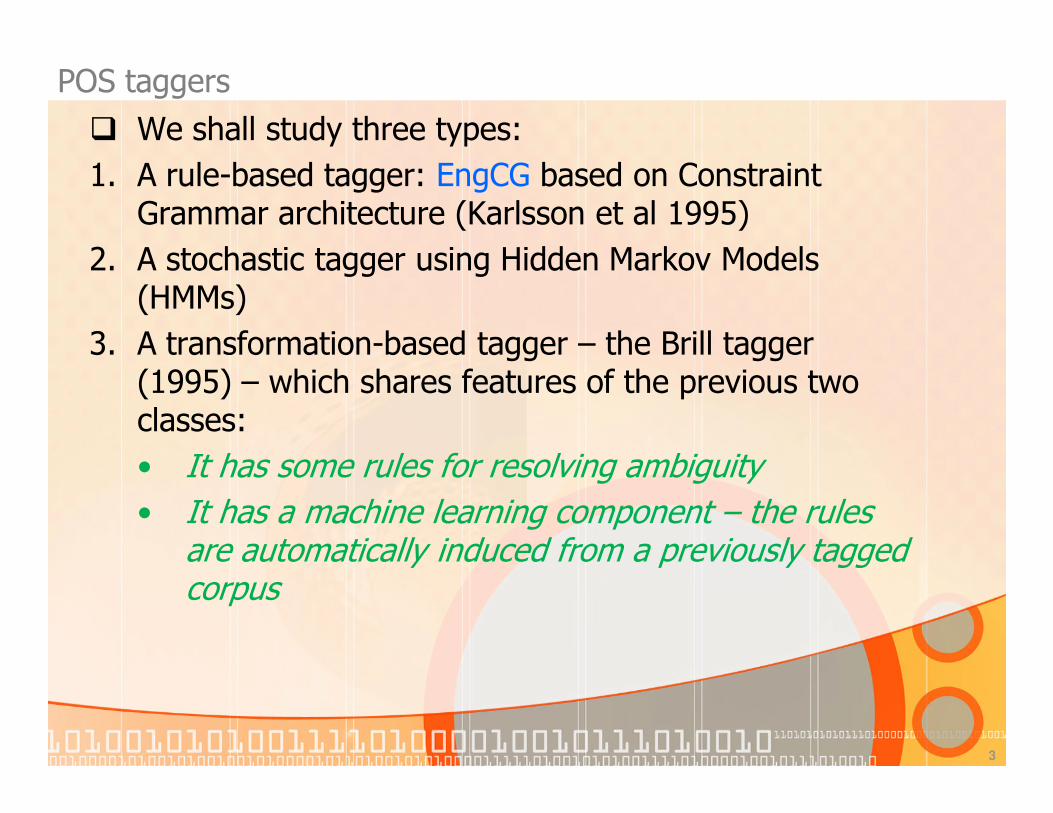
� We shall study three types:
1. A rule-based tagger: EngCG based on Constraint Grammar architecture (Karlsson et al 1995)
2. A stochastic tagger using Hidden Markov Models (HMMs)
3. A transformation-based tagger – the Brill tagger (1995) – which shares features of the previous two classes:
• It has some rules for resolving ambiguity
• It has a machine learning component – the rules are automatically induced from a previously tagged corpus
10/16/2011 Speech and Language Processing - Jurafsky and Martin
4
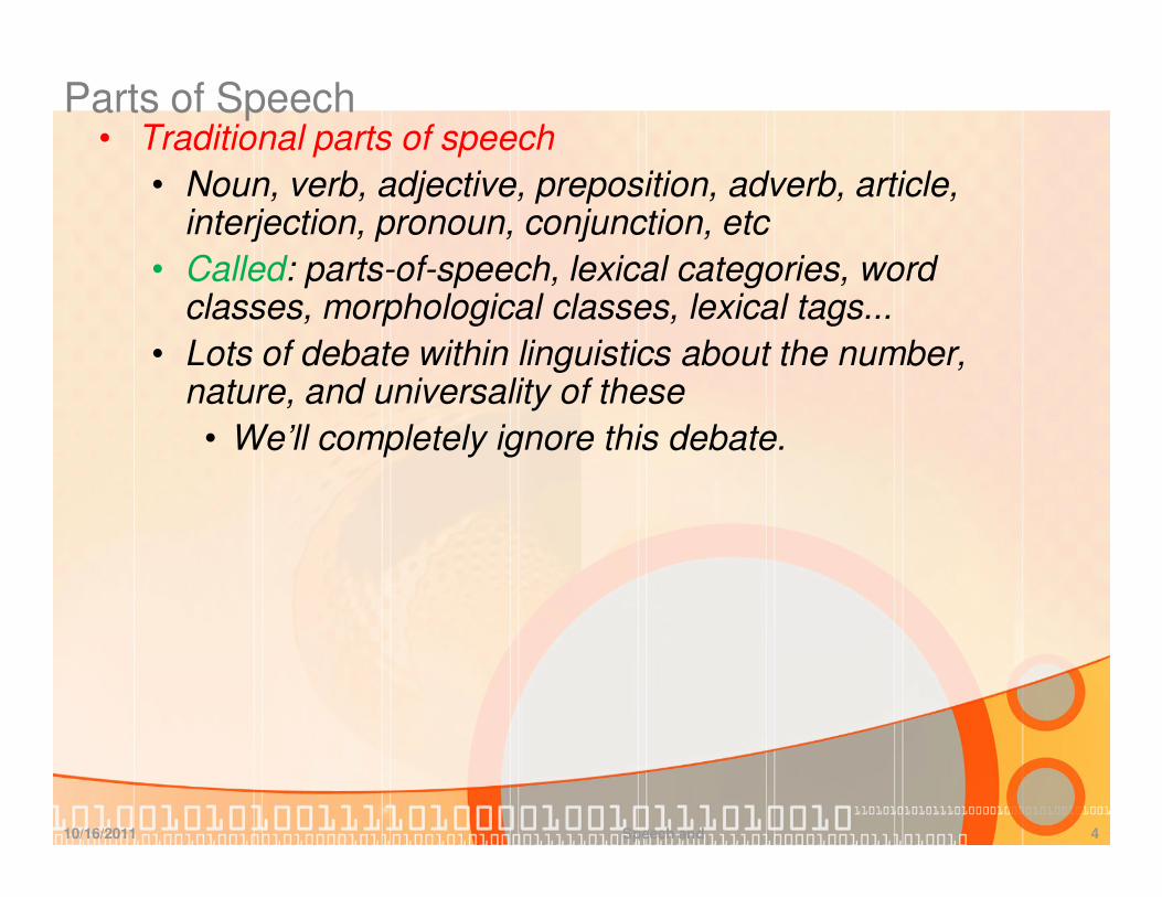
Parts of Speech• Traditional parts of speech
• Noun, verb, adjective, preposition, adverb, article, interjection, pronoun, conjunction, etc
• Called: parts-of-speech, lexical categories, word classes, morphological classes, lexical tags...
• Lots of debate within linguistics about the number, nature, and universality of these
• We’ll completely ignore this debate.
10/16/2011 Speech and Language Processing - Jurafsky and Martin
5
POS examples
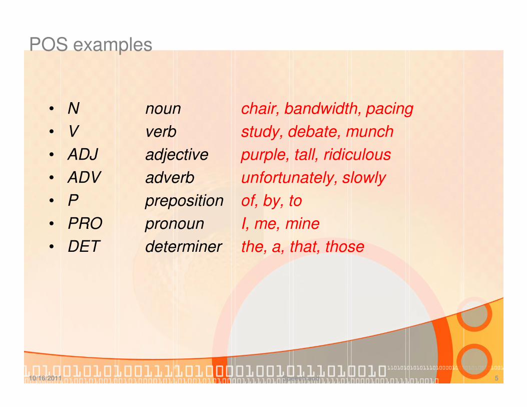
• N noun chair, bandwidth, pacing
• V verb study, debate, munch
• ADJ adjective purple, tall, ridiculous
• ADV adverb unfortunately, slowly
• P preposition of, by, to
• PRO pronoun I, me, mine
• DET determiner the, a, that, those

10/16/2011 Speech and Language Processing - Jurafsky and Martin
6
POS Tagging
• The process of assigning a part-of-speech or lexical class marker to each word in a collection.
WORD tag
the DET
koala N
put V
the DET
keys N
on P
the DET
table N
10/16/2011 Speech and Language Processing - Jurafsky and Martin
7
Why is POS Tagging Useful?
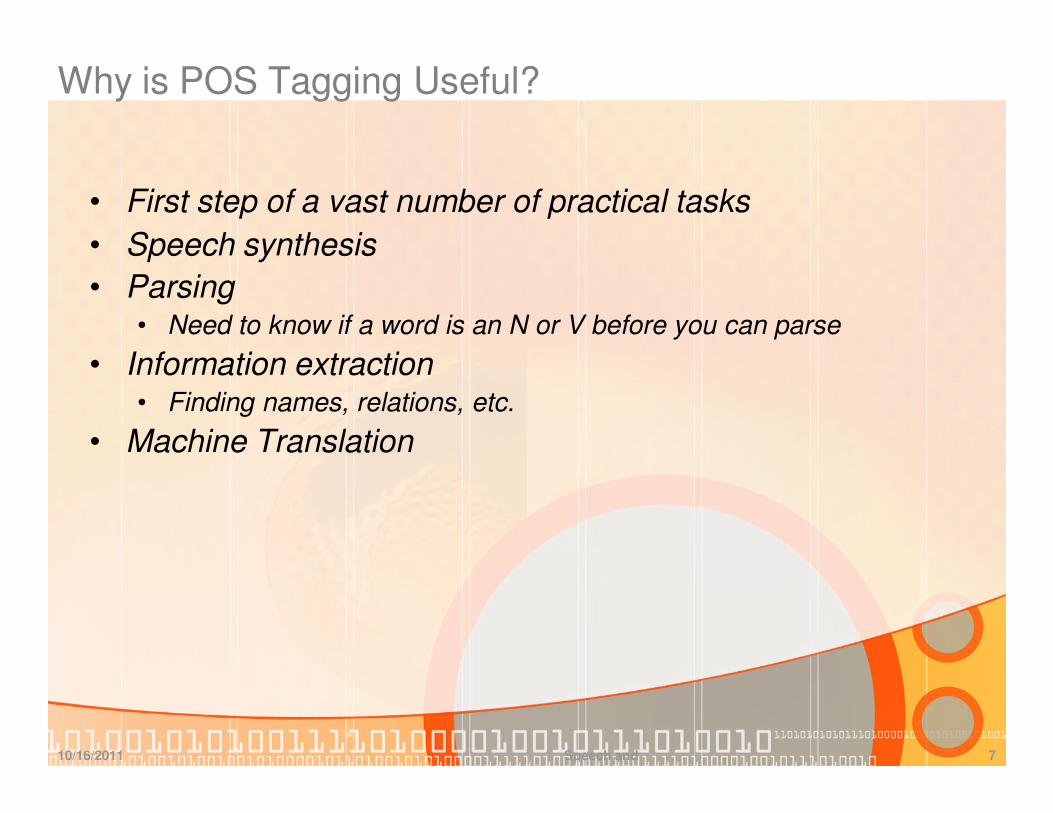
• First step of a vast number of practical tasks
• Speech synthesis
• Parsing• Need to know if a word is an N or V before you can parse
• Information extraction• Finding names, relations, etc.
• Machine Translation

10/16/2011 Speech and Language Processing - Jurafsky and Martin
8
Open and Closed Classes
• Closed class: a small fixed membership
• Prepositions: of, in, by, …
• Auxiliaries: may, can, will had, been, …
• Pronouns: I, you, she, mine, his, them, …
• Usually function words (short common words which play a role in grammar)
• Open class: new ones can be created all the time
• English has 4: Nouns, Verbs, Adjectives, Adverbs
• Many languages have these 4, but not all!
10/16/2011 Speech and Language Processing - Jurafsky and Martin
9
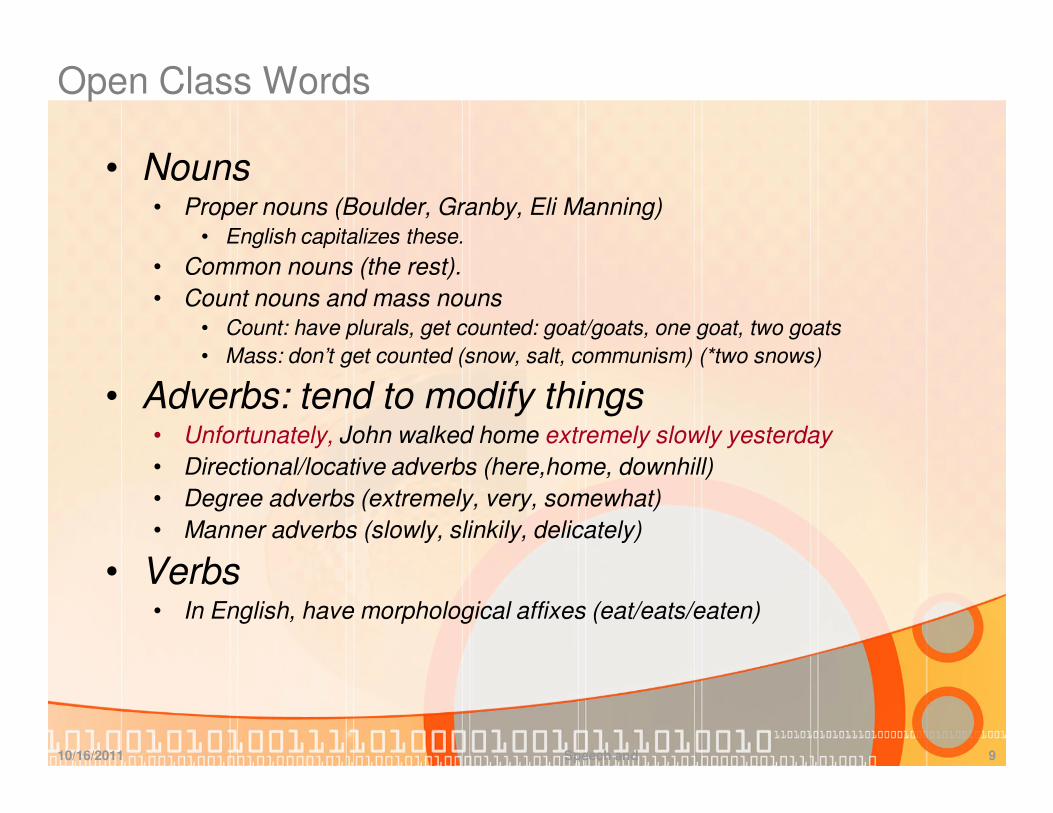
Open Class Words
• Nouns• Proper nouns (Boulder, Granby, Eli Manning)
• English capitalizes these.
• Common nouns (the rest).
• Count nouns and mass nouns• Count: have plurals, get counted: goat/goats, one goat, two goats
• Mass: don’t get counted (snow, salt, communism) (*two snows)
• Adverbs: tend to modify things• Unfortunately, John walked home extremely slowly yesterday
• Directional/locative adverbs (here,home, downhill)
• Degree adverbs (extremely, very, somewhat)
• Manner adverbs (slowly, slinkily, delicately)
• Verbs• In English, have morphological affixes (eat/eats/eaten)

10/16/2011 Speech and Language Processing - Jurafsky and Martin
10
Closed Class WordsExamples:
• prepositions: on, under, over, …
• particles: up, down, on, off, …
• determiners: a, an, the, …
• pronouns: she, who, I, ..
• conjunctions: and, but, or, …
• auxiliary verbs: can, may should, …
• numerals: one, two, three, third, …
10/16/2011 Speech and Language Processing - Jurafsky and Martin
11
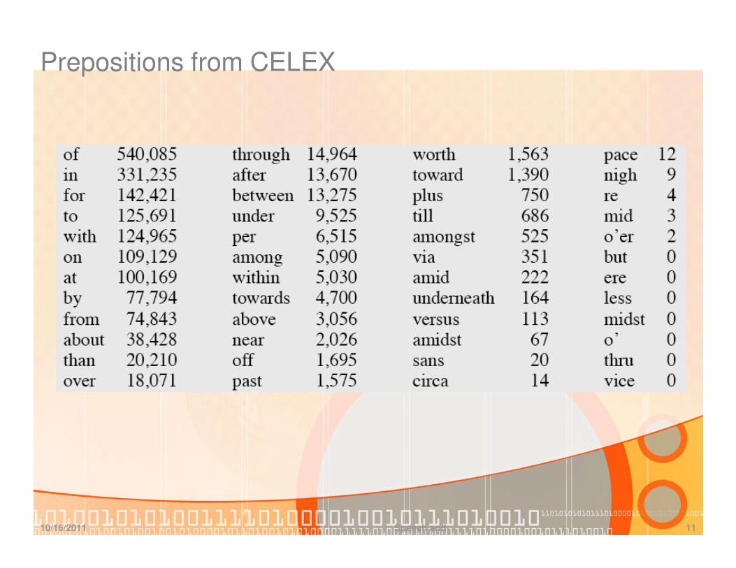
Prepositions from CELEX

10/16/2011 Speech and Language Processing - Jurafsky and Martin
12
English Particles

10/16/2011 Speech and Language Processing - Jurafsky and Martin
13
Conjunctions

10/16/2011 Speech and Language Processing - Jurafsky and Martin
14
POS Tagging-- Choosing a Tagset
• There are so many parts of speech, potential distinctions we can draw
• To do POS tagging, we need to choose a standard set of tags to work with
• Could pick very coarse tagsets
• N, V, Adj, Adv.
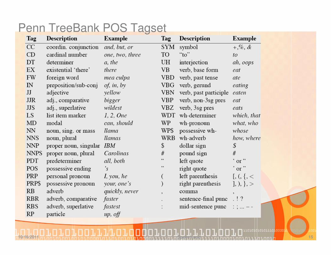
• More commonly used set is finer grained, the “Penn TreeBank tagset”, 45 tags
• PRP$, WRB, WP$, VBG
• Even more fine-grained tagsets exist
10/16/2011 Speech and Language Processing - Jurafsky and Martin
15
Penn TreeBank POS Tagset

10/16/2011 Speech and Language Processing - Jurafsky and Martin
16
Using the Penn Tagset
• The/DT grand/JJ jury/NN commmented/VBD on/IN a/DT number/NN of/IN other/JJ topics/NNS ./.
• Prepositions and subordinating conjunctions marked IN (“although/IN I/PRP..”)
• Except the preposition/complementizer “to” is just marked “TO”.

10/16/2011 Speech and Language Processing - Jurafsky and Martin
17
POS Tagging
• Words often have more than one POS: back
• The back door = JJ
• On my back = NN
• Win the voters back = RB
• Promised to back the bill = VB
• The POS tagging problem is to determine the POS tag for a particular instance of a word.
These examples from Dekang Lin

10/16/2011 Speech and Language Processing - Jurafsky and Martin
18
How Hard is POS Tagging? Measuring Ambiguity

10/16/2011 Speech and Language Processing - Jurafsky and Martin
19
Rule-Based Tagging
• Start with a dictionary
• Assign all possible tags to words from the dictionary
• Write rules by hand to selectively remove tags
• Leaving the correct tag for each word.

10/16/2011 Speech and Language Processing - Jurafsky and Martin
20
Start With a Dictionary
• she: PRP
• promised: VBN,VBD
• to TO
• back: VB, JJ, RB, NN
• the: DT
• bill: NN, VB
• Etc… for the ~100,000 words of English with more than 1 tag

10/16/2011 Speech and Language Processing - Jurafsky and Martin
21
Assign Every Possible Tag
NN
RB
VBN JJ VB
PRP VBD TO VB DT NN
She promised to back the bill

10/16/2011 Speech and Language Processing - Jurafsky and Martin
22
Write Rules to Eliminate Tags
Eliminate VBN if VBD is an option when VBN|VBD follows “<start> PRP”
NN
RB
JJ VB
PRP VBD TO VB DT NN
She promised to back the bill
VBN

10/16/2011 Speech and Language Processing - Jurafsky and Martin
23
Stage 1 of ENGTWOL Tagging
• First Stage: Run words through FST morphological analyzer to get all parts of speech.
• Example: Pavlov had shown that salivation …
Pavlov PAVLOV N NOM SG PROPERhad HAVE V PAST VFIN SVO
HAVE PCP2 SVOshown SHOW PCP2 SVOO SVO SVthat ADV
PRON DEM SGDET CENTRAL DEM SGCS
salivation N NOM SG

10/16/2011 Speech and Language Processing - Jurafsky and Martin
24
Stage 2 of ENGTWOL Tagging
• Second Stage: Apply NEGATIVE constraints.
• Example: Adverbial “that” rule
• Eliminates all readings of “that” except the one in
• “It isn’t that odd”
Given input: “that”If
(+1 A/ADV/QUANT) ;if next word is adj/adv/quantifier
(+2 SENT-LIM) ;following which is E-O-S
(NOT -1 SVOC/A) ; and the previous word is not a
; verb like “consider” which
; allows adjective complements
; in “I consider that odd”
Then eliminate non-ADV tagsElse eliminate ADV

25
Rule-based Tagging 1/2
• Phase 1: assign to each word a list of potential parts-of-speech by looking up a dictionary.
• Phase 2: use if-then rules to pinpoint the correct tag for each word.
Example:Pavlov had shown that salivation ...
Phase 1

26
Rule-based Tagging 2/2
Example:Pavlov had shown that salivation ...
Phase 2
Phase 2: apply a large set of constraints (3744 in the EngCG-2 system ofVoutilainen 1999) to rule out incorrect POS

10/16/2011 Speech and Language Processing - Jurafsky and Martin
27
Hidden Markov Model Tagging
• Using an HMM to do POS tagging is a special case of Bayesian inference
• Foundational work in computational linguistics
• Bledsoe 1959: OCR
• Mosteller and Wallace 1964: authorship identification
• It is also related to the “noisy channel” model that’s the basis for ASR, OCR and MT
10/16/2011 Speech and Language Processing - Jurafsky and Martin
28
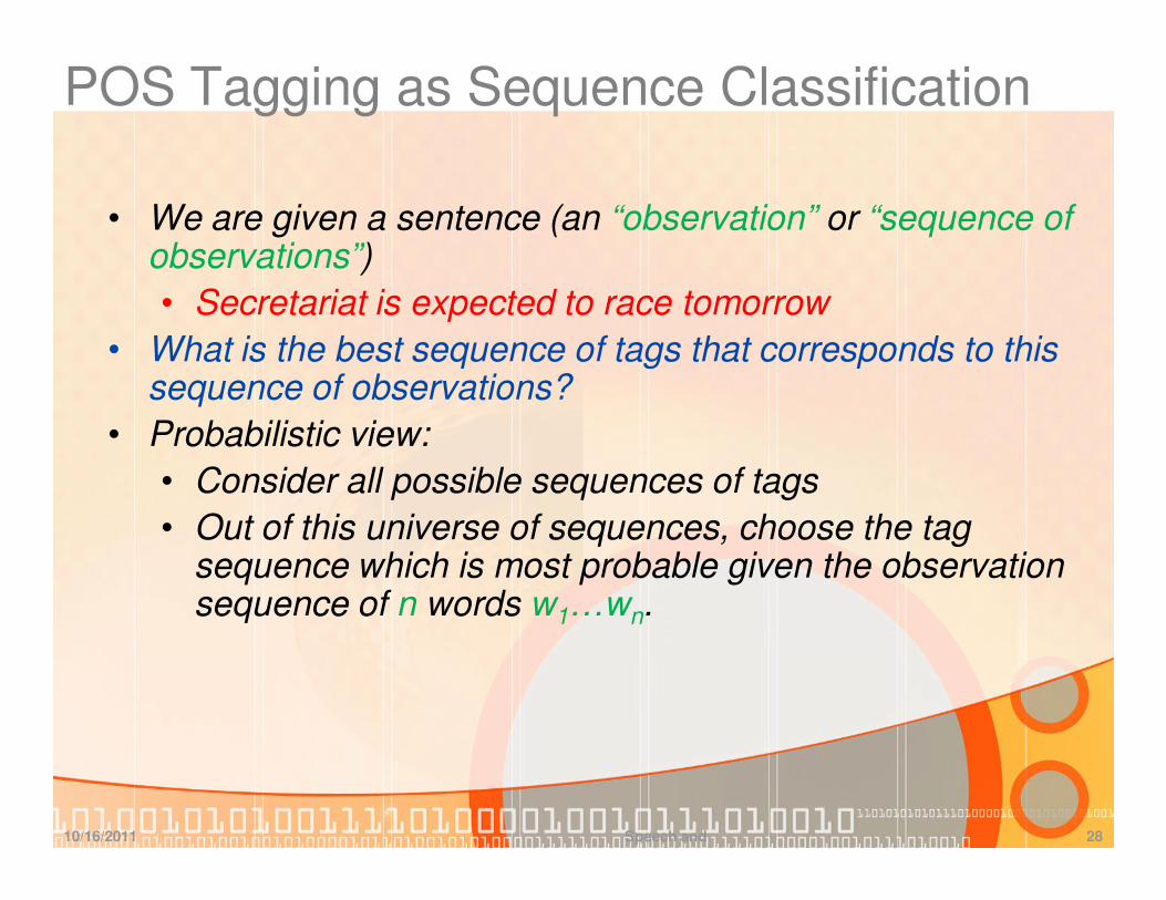
POS Tagging as Sequence Classification
• We are given a sentence (an “observation” or “sequence of observations”)
• Secretariat is expected to race tomorrow
• What is the best sequence of tags that corresponds to this sequence of observations?
• Probabilistic view:
• Consider all possible sequences of tags
• Out of this universe of sequences, choose the tag sequence which is most probable given the observation sequence of n words w1…wn.

10/16/2011 Speech and Language Processing - Jurafsky and Martin
29
Getting to HMMs
• We want, out of all sequences of n tags t1…tn the single tag sequence such that P(t1…tn|w1…wn) is highest.
• Hat ^ means “our estimate of the best one”
• Argmaxx f(x) means “the x such that f(x) is maximized”
)|(maxargˆ nn
t
nwtPt
n111
1
=

10/16/2011 Speech and Language Processing - Jurafsky and Martin
30
Getting to HMMs
• This equation is guaranteed to give us the best tag sequence
• But how to make it operational? How to compute this value?
• Intuition of Bayesian classification:
• Use Bayes rule to transform this equation into a set of other probabilities that are easier to compute
)|(maxargˆ nn
t
n wtPtn
111
1
=

10/16/2011 Speech and Language Processing - Jurafsky and Martin
31
Using Bayes Rule
)|(maxargˆ nn
t
n wtPtn
111
1
=

10/16/2011 Speech and Language Processing - Jurafsky and Martin
32
Likelihood and Prior
∏=
−≈n
i
ii
nttPtP
1
11 )|()(

33
HMM simplifying assumptions
• It is too hard to compute
� Assumption 1: the probability of a word is dependent only on its part-of-speech, not on the surrounding words or other tags around it.
� Assumption 2: the probability of a tag appearing is dependent only on the previous tag (bigram assumption)
87648476prior
n
likelihood
nn
t
ntPtwPt
n
)()|(maxargˆ1111
1
=
∏≈=
n
iii
nn twPtwP1
11 )|()|(
∏=
−≈n
i
ii
n ttPtP1
11 )|()(
∏≈==
−
n
iiiii
t
nn
t
nttPtwPwtPt
nn 1
1111
11
)|()|(maxarg)|(maxargˆ
Tag-transitionprobabilities
Wordlikelihoods

10/16/2011 Speech and Language Processing - Jurafsky and Martin
34
Two Kinds of Probabilities
• Tag transition probabilities p(ti|ti-1)
• Determiners likely to precede adjs and nouns
• That/DT flight/NN
• The/DT yellow/JJ hat/NN
• So we expect P(NN|DT) and P(JJ|DT) to be high
• But P(DT|JJ) to be:
• Compute P(NN|DT) by counting in a labeled corpus:

10/16/2011 Speech and Language Processing - Jurafsky and Martin
35
Two Kinds of Probabilities
• Word likelihood probabilities p(wi|ti)
• VBZ (3sg Pres verb) likely to be “is”
• Compute P(is|VBZ) by counting in a labeled corpus:
36
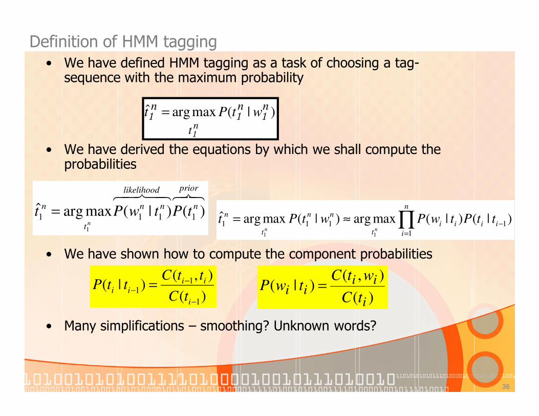
Definition of HMM tagging
• We have defined HMM tagging as a task of choosing a tag-sequence with the maximum probability
• We have derived the equations by which we shall compute the probabilities
• We have shown how to compute the component probabilities
• Many simplifications – smoothing? Unknown words?
)|(maxargˆ nn
t
nwtPt
n111
1
=
87648476 prior
n
likelihood
nn
t
n tPtwPtn
)()|(maxargˆ1111
1
=∏
=
−≈=n
i
iiiit
nn
t
n ttPtwPwtPtnn
1
1111 )|()|(maxarg)|(maxargˆ
11
)(
),()|(
1
11
−
−− =
i
iiii
tC
ttCttP
)(
),()|(
i
iiii
tC
wtCtwP =

10/16/2011 Speech and Language Processing - Jurafsky and Martin
37
Example: The Verb “race”
• Secretariat/NNP is/VBZ expected/VBN to/TO race/VBtomorrow/NR
• People/NNS continue/VB to/TO inquire/VB the/DTreason/NN for/IN the/DT race/NN for/IN outer/JJ space/NN
• How do we pick the right tag?

10/16/2011 Speech and Language Processing - Jurafsky and Martin
38
Disambiguating “race”

10/16/2011 Speech and Language Processing - Jurafsky and Martin
39
Example• P(NN|TO) = .00047
• P(VB|TO) = .83
• P(race|NN) = .00057
• P(race|VB) = .00012
• P(NR|VB) = .0027
• P(NR|NN) = .0012
• P(VB|TO)P(NR|VB)P(race|VB) = .00000027
• P(NN|TO)P(NR|NN)P(race|NN)=.00000000032
• So we (correctly) choose the verb reading,

10/16/2011 Speech and Language Processing - Jurafsky and Martin
40
Hidden Markov Models
• What we’ve described with these two kinds of probabilities is a Hidden Markov Model (HMM)

10/16/2011 Speech and Language Processing - Jurafsky and Martin
41
Definitions• A weighted finite-state automaton adds
probabilities to the arcs• The sum of the probabilities leaving any arc must
sum to one
• A Markov chain is a special case of a WFST in which the input sequence uniquely determines which states the automaton will go through
• Markov chains can’t represent inherently ambiguous problems• Useful for assigning probabilities to unambiguous
sequences

42
Formalizing Hidden Markov Model taggers
• HMM is an extension of finite automata
� A FSA is defined by a set of states + a set of transitions between states that are taken based on observations.
• A weighted finite-state automaton is an augmentation of the FSA in which the arcs are associated with a probability – indicating how likely that path is to be taken.
q1
q2
q7
q6q3
q5
q0
q8
a
a
a
q4
q9
a a
a
bb
b
b
b
b b
a
FSAInput: aab
a
b
q1
q2
q7
q6q3
q5
q0
q8
a
a
a
q4
q9
a a
a
bb
b
b
b
b b
a
WFSAInput: aab
0.3
0.7
0.5
0.5
0.8
0.2
0.4
0.6 0.3
0.7
0.9
0.10.8
0.2
a
b
0.4
0.6
A Markov Chain=special WFSA
The input sequenceDetermines whichStates the WFSA willGo through.

43
Hidden Markov Model (HMM) 1/4
• A Markov chain – Markov model – appropriate for situations in which we can observe the conditioning events – it is not appropriate for POS tagging:
�We observe the words in the input
�We do not observe the POS tags in the input• We cannot condition any probability on the previous POS tag
• A Hidden Markov Model allows us to describe both observedevents and hidden events that we think of as causal factorsfor the probabilistic model.
• A HMM is defined by:
• A set of states Q
• A set of transition probabilities A
• A set of observation likelihoods B
• A defined start state and end state
• A set of observation symbols O

44
Hidden Markov Model (HMM) 2/4
• Parameters that define HMMs:
� states :a set of states Q= q1q2…qN� transition probabilities: a transition probability matrix A=[aij]…,
where aij… represents the probability to move from state i to state j, while Σj=1
naij=1
� Observations O=o1,o2,…oT: a sequence of observations, each drawn from a vocabulary V=v1, v2, …, vV.
� Sequence of observation likelihoods B=bi(ot): also known as
emission probabilities (B=bi(ot)), each expressing the probability of an observation ot being generated from a state i. To express such
probabilities, a set of observation symbols O=o1, o2 … oT are used.
� Q0, qF: a special start state and final state that are not associated with observations, as well as transition probabilities a01a02a03…a0n our of the start state and a1Fa2F…anF into the end state.
45
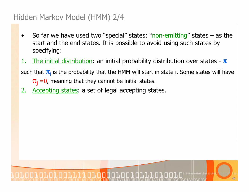
Hidden Markov Model (HMM) 2/4
• So far we have used two “special” states: “non-emitting” states – as the start and the end states. It is possible to avoid using such states by specifying:
1. The initial distribution: an initial probability distribution over states - ππππ
such that πi is the probability that the HMM will start in state i. Some states will have
πj =0, meaning that they cannot be initial states.
2. Accepting states: a set of legal accepting states.

46
Hidden Markov Model (HMM) 3/4• An HMM has observed states and hidden states.
• Two kinds of probabilities: A transition probabilities and Bobservation probabilities. They correspond to the prior and likelihood probabilities.
87648476prior
n
likelihood
nn
t
n tPtwPtn
)()|(maxargˆ1111
1
=
∏≈==
−
n
iiiii
t
nn
t
n ttPtwPwtPtnn 1
1111
11
)|()|(maxarg)|(maxargˆ
Wordlikelihoods
Tag transitionprobabilities
Markov Chain for the hidden states
The A transition probabilitiesare used to compute the prior probabilities

47
Hidden Markov Model (HMM) 4/4
• A different view of HMMs, focused on word likelihoods B.

10/16/2011 Speech and Language Processing - Jurafsky and Martin
48
Definitions and examples!!!
• A weighted finite-state automaton adds probabilities to the arcs• The sum of the probabilities leaving any arc must
sum to one
• A Markov chain is a special case of a WFST in which the input sequence uniquely determines which states the automaton will go through
• Markov chains can’t represent inherently ambiguous problems• Useful for assigning probabilities to unambiguous
sequences – some examples!!!

10/16/2011 Speech and Language Processing - Jurafsky and Martin
49
Markov Chain for Weather

10/16/2011 Speech and Language Processing - Jurafsky and Martin
50
Markov Chain for Words

10/16/2011 Speech and Language Processing - Jurafsky and Martin
51
Markov Chain: “First-order observable Markov Model”
• A set of states
• Q = q1, q2…qN; the state at time t is qt
• Transition probabilities:
• a set of probabilities A = a01a02…an1…ann.
• Each aij represents the probability of transitioning from state i to state j
• The set of these is the transition probability matrix A
• Current state only depends on previous state
P(qi | q1...qi−1) = P(qi | qi−1)

10/16/2011 Speech and Language Processing - Jurafsky and Martin
52
Markov Chain for Weather
• What is the probability of 4 consecutive rainy days?
• Sequence is rainy-rainy-rainy-rainy
• I.e., state sequence is 3-3-3-3
• P(3,3,3,3) =
• π3a33a33a33a33 = 0.2 x (0.6)3 = 0.0432
State 1 State 2 State 3
0.5 0.3 0.2π
State 1 State 2 State 3 State 4
State 0 0.5 0.3 0.2
State 1 0.6 0.1 0.2 0.1
State 2 0.2 0.4 0.3 0.1
State 3 0.1 0.2 0.6 0.1
A

10/16/2011 Speech and Language Processing - Jurafsky and Martin
53
HMM for Ice Cream
• You are a climatologist in the year 2799
• Studying global warming
• You can’t find any records of the weather in Baltimore, MA for summer of 2007
• But you find Jason Eisner’s diary
• Which lists how many ice-creams Jason ate every date that summer
• Our job: figure out how hot it was

10/16/2011 Speech and Language Processing - Jurafsky and Martin
54
Hidden Markov Model
• For Markov chains, the output symbols are the same as the states.• See hot weather: we’re in state hot
• But in part-of-speech tagging (and other things)• The output symbols are words
• But the hidden states are part-of-speech tags
• So we need an extension!
• A Hidden Markov Model is an extension of a Markov chain in which the input symbols are not the same as the states.
• This means we don’t know which state we are in.

10/16/2011 55
• States Q = q1, q2…qN;
• Observations O= o1, o2…oN;
• Each observation is a symbol from a vocabulary V = {v1,v2,…vV}
• Transition probabilities• Transition probability matrix A = {aij}
• Observation likelihoods• Output probability matrix B={bi(k)}
• Special initial probability vector π
π i = P(q1 = i) 1≤ i ≤ N
aij = P(qt = j | qt−1 = i) 1 ≤ i, j ≤ N
bi(k) = P(X t = ok | qt = i)
Hidden Markov Models

10/16/2011 Speech and Language Processing - Jurafsky and Martin
56
Eisner Task• Given
• Ice Cream Observation Sequence: 1,2,3,2,2,2,3…
• Produce:
• Weather Sequence: H,C,H,H,H,C…

10/16/2011 Speech and Language Processing - Jurafsky and Martin
57
HMM for Ice Cream
bi(k) = P(X t = ok | qt = i)
Output probability matrix B={bi(k)}

10/16/2011 Speech and Language Processing - Jurafsky and Martin
58
Transition Probabilities
Back to POS tagging

10/16/2011 Speech and Language Processing - Jurafsky and Martin
59
Observation Likelihoods

10/16/2011 Speech and Language Processing - Jurafsky and Martin
60
Decoding
• Ok, now we have a complete model that can give us what we need. Recall that we need to get
• We could just enumerate all paths given the input and use the model to assign probabilities to each.• Not a good idea.
• Luckily dynamic programming (last seen in Ch. 3 with minimum edit distance) helps us here

61
The Viterbi Algorithm for HMMs 1/6
• For any model that contains hidden variables, the task of determining which sequence of variables is the underlying source of some sequence of observations is called the decoding task.
• The most common decoding algorithm for HMMs is the Viterbi algorithm.
• It is a standard application of dynamic programming – looks a lot like minimum edit distance.
� THE VITERBI ALGORITHM
• INPUT: (1) a single HMM and (2) a set of observed words o=(o1, o2, …ot)
• OUTPUT: (1) the most probable state/tag sequence q=(q1, q2 … qt) together with (2) its probability.

62
The Viterbi Algorithm for HMMs 2/6� THE VITERBI ALGORITHM
• INPUT: (1) a single HMM and (2) a set of observed words o=(o1, o2, …ot)
• OUTPUT: (1) the most probable state/tag sequence q=(q1, q2 … qt) together with (2) its probability.
� Let us define the HMM by two tables:
1. The tag-transition probability table A
2. The observation likelihoods B array
A B
A HMM is defined by:A set of states QA set of transition probabilitiesAA set of observation likelihoodsBA defined start state and end stateA set of observation symbols O

63
The Viterbi Algorithm for HMMs 3/6� THE tag transition probability table A
<s>
PPSS
TO
VB
NN
</s>

64
The Viterbi Algorithm for HMMs 4/6� THE observation likelihood array B
<s>
PPSS
TO
VB
NN
</s>
B1P(want|VB)=0.093P(race|VB)=0.00012
B2P(to|TO)=0.99
B3P(want|NN)=0.00054P(race|NN)=0.00057
B4P(I|PPS)=0.37

The Viterbi Algorithm for HMMs 6/6
65

66
The Viterbi Algorithm for HMMs 5/6� How it works? It builds a probability matrix:
5 end
4 NN 0.41×1.0×0
=0
.0045×0.25×000054
.0012×.000051×0=0
3 TO 0.042×1.0×
0=0
.00079×.25×0=0
.83×.000051×.99
2 VB 0.019×1.0×
0=0
0.23×0.25×
0.093=
.000051
.0038×.000051×0=0
1 PPSS 0.067×1.0×
0.37=0.25
.00014×.25×0=0
.007×.000051×0=0
0 start 1.0
# I want to race #
0 1 2 3 4 5
One row for each state One column for each observation
exercise
exercise
The Viterbi value=The product of:1. The transition probabilityA[I,j]2. Previous path probabilityViterbi[s’,t-1]3. Observation likelihoodBs[ot]
Observations likelihoods (Brown corpus)Tag Transition Probabilities (Brown corpus)

67
Extending HMMs to trigrams 1/2
• Previous assumption: the tag appearing is dependent only on the previous tag
• Most modern HMM taggers use a little more history – the previous two tags
• The state-of-the-art HMM tagger of Brants(2000) uses the location of the end of sentence. Dependence on the end-of-sequence is represented as tn+1. POS tagging is done by:
∏=
−≈n
i
ii
n ttPtP1
11 )|()(
∏≈=
−−
n
iiii
n tttPtP1
211 ),|()(
)|(),|()|(maxarg)|(maxargˆnn
n
iiiiii
t
nn
t
n ttPtttPtwPwtPtnn
1
1
21111
11
+=
−−
∏≈=
One problem: data sparsity

68
Deleted interpolation 1/2
• Compute the trigram probability with MLE from counts:
Many of these counts will be 0!
• Solution: estimate the probability by combining more robust but weaker estimators. E.g if we never seen PRP VB TO, we cannot compute P(TO|PRP, VB) but we can compute P(TO|VB) or even P(TO).
:),(
),,(),|(
12
1221
−−
−−−− =
ii
iiiiii
ttC
tttCtttP
N
tCtP
tC
ttCttP
ttC
tttCtttP
ii
i
iiii
ii
iiiiii
)()(ˆ Unigrams
)(
),()|(ˆ Bigrams
),(
),,(),|(ˆ Trigrams
1
11
12
1221
=
=
=
−
−−
−−
−−
−−
Maximum Likelihood Estimation
How should they be combined???
)(ˆ)|(ˆ)|(ˆ)|( 31221121 iiiiiiiii tPttPtttPtttP λλλ ++= −−−−−

Deleted Interpolation 2/2
69

10/16/2011 Speech and Language Processing - Jurafsky and Martin
70
The Viterbi Algorithm

10/16/2011 Speech and Language Processing - Jurafsky and Martin
71
Viterbi Example

10/16/2011 Speech and Language Processing - Jurafsky and Martin
72
Viterbi Summary
• Create a matrix
• With columns corresponding to inputs
• Rows corresponding to possible states
• Sweep through the array in one pass filling the columns left to right using our transition probabilities and observations probabilities
• Dynamic programming key is that we need only store the MAX probability path to each cell, (not all paths).

73
Transformation-Based Tagging
• Is based on transformation-based learning
• It is a supervised learning technique – it assumed a pre-tagged corpus
� The TBL algorithm has a set of tagging rules
� The corpus is first tagged using the broadest rule (the one that applies to most cases)
• Then, a more specific rule is applied – it changes the original tags.
• Next, an even narrower rule is applied, which changes a smaller number of tags. Some of these tags might have been previously changed.

74
How TBL rules are applied
• Before rules are applied, the tagger labels every word with its most-likely tags from a corpus. E.g. in the Brown corpus, “race” is most likely tagged to be a noun:
• This means that:
1. … is/VBZ expected/VBN to/TO race/NN tomorrow/NN.
2. … the/DT reason/NN for/IN the/DT race/NN for/IN outer/JJ space/NN.
� After selecting the most likely tag, Brill’s tagger applies its transformation rules. E.g. it learned a rule:
� Change NN to VB when the previous tag is TO
� It changes … is/VBZ expected/VBN to/TO race/NN tomorrow/NN into
… is/VBZ expected/VBN to/TO race/VB tomorrow/NN
02.0)|(
98.0)|(
=
=
raceVBP
raceNNP
incorrect
correct

75
How TBL rules are learned
• Brill’s tagger has three major stages:
1. It labels every word with its most-likely tag.
2. It examines every possible transformation and selects the one that results in the most improved tagging
3. It re-tags the data according to this rule. Repeat 2-3 until some stopping criterion. Eg. insufficient improvement.
• The output of the TBL process is an ordered list of transformations. They constitute the “tagging procedure” that can be applied to a new corpus.
• In principle, the possible set of transformations in infinite. The algorithms needs a way to limit the set of transformations in order to pick the best one to pass to the algorithm.
• Solution – design a small set of templates. Every transformation is an instantiation of a template.

76
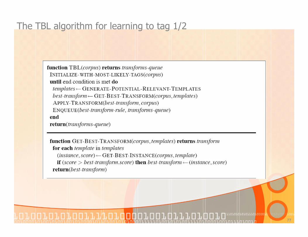
77
The TBL algorithm for learning to tag 1/2
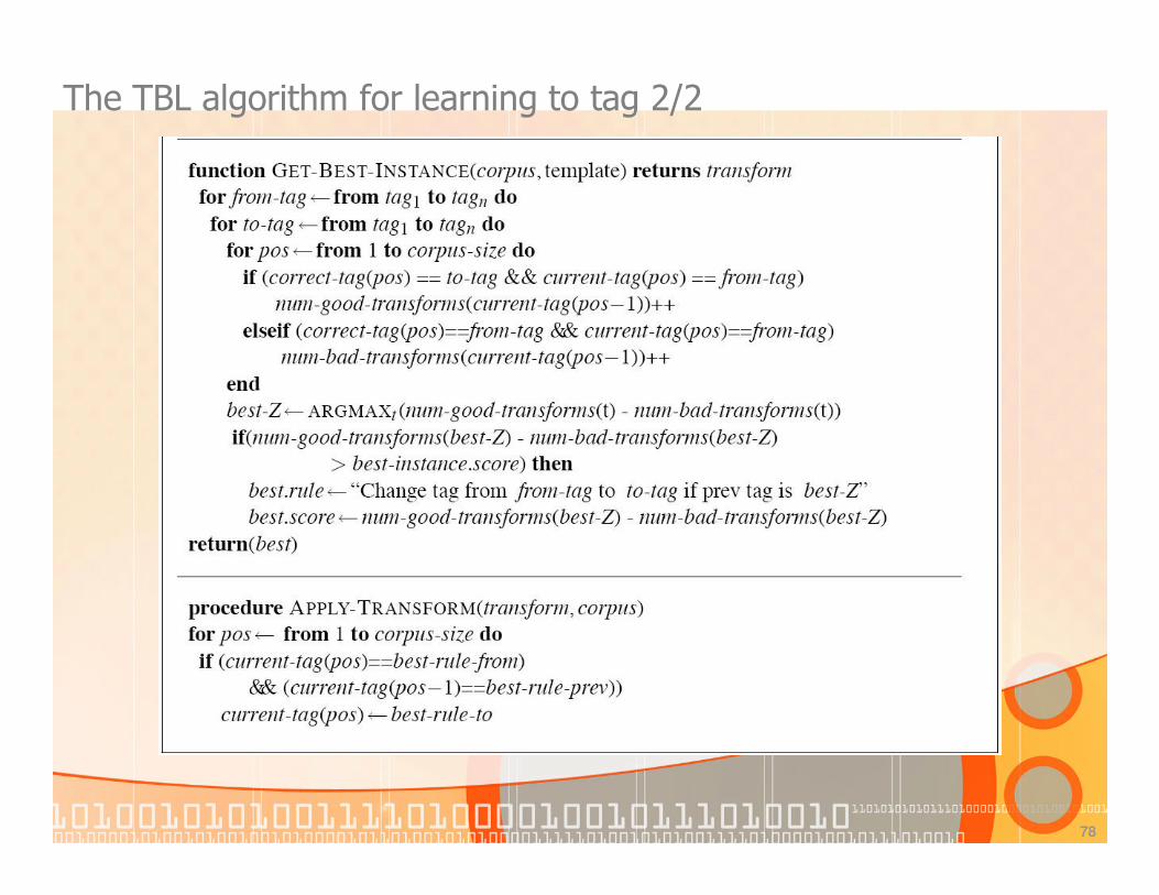
The TBL algorithm for learning to tag 2/2
78

79
Unknown words 1/2
• Make use of the morphology of words
• Four methods:
1. Weischedel et al (1993) built a model based on 4 kinds of morphological and orthographic features
• Used 3 inflectional endings (-ed, -s, -ing), 32 derivational endings (e.g. –ion, -al, -ive and –ly), 4 values of capitalization depending on whether the word is sentence initial and whether the word was hyphenated.
• For each feature, they have trained maximum likelihood estimates. The features were combined to estimate a probability:
2. HMM-based approach Brants (2000) generalizes the use of morphology in a data-driven way. Consider suffixes up to ten letters and compute the probability of the tag given the suffix
)|pthendings/hy()|capital()|word-unkown()|( iiiii tptptptwP ××=
)...|( 1 nini lltP +−

80
Unknown words 2/2
3. Non-HMM approach based on TBL (Brill 1995) where the available templates were defined orthographically (e.g. the first N letters of the word, the last N letters of the word)
4. Maximum-entropy approach due to Rathnaparkhi (1996). For each word it includes suffixes and prefixes of length < 4. Log-linear model Toutanova (2003) augments the Rathnaparkhi features with an all-caps feature and a company name detector.

10/16/2011 Speech and Language Processing - Jurafsky and Martin
81
Evaluation• So once you have you POS tagger running how do you
evaluate it?
• Overall error rate with respect to a gold-standard test set.
• Error rates on particular tags
• Error rates on particular words
• Tag confusions...
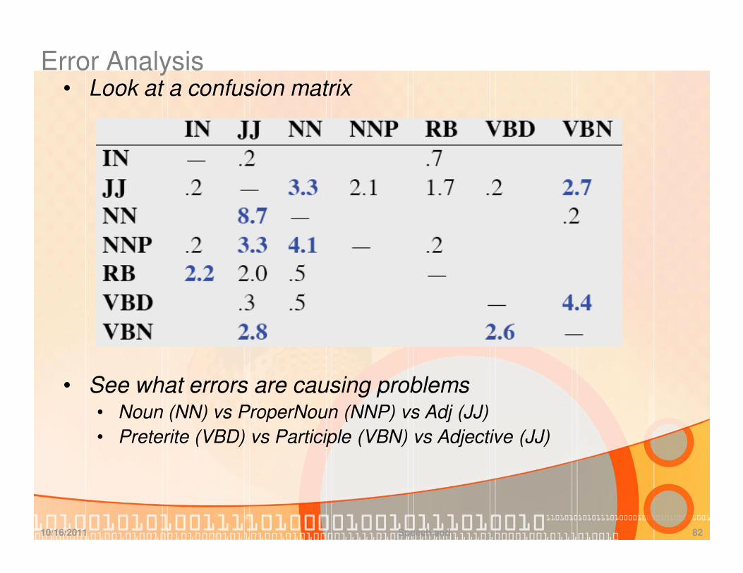
• Confusion matrix: a cell (x, y) contains the number of times an item with correct classification x was by the model as y.
10/16/2011 Speech and Language Processing - Jurafsky and Martin
82
Error Analysis• Look at a confusion matrix
• See what errors are causing problems• Noun (NN) vs ProperNoun (NNP) vs Adj (JJ)
• Preterite (VBD) vs Participle (VBN) vs Adjective (JJ)

10/16/2011 Speech and Language Processing - Jurafsky and Martin
83
Evaluation• The result is compared with a manually coded “Gold
Standard”
• Typically accuracy reaches 96-97%
• This may be compared with result for a baseline tagger (one that uses no context).
• Important: 100% is impossible even for human annotators.