v. debt sustainability analysis. debt sustainability analysis ... integrated by a stochastic...

MINISTERO DELL’ECONOMIA E DELLE FINANZE 64

V. DEBT SUSTAINABILITY ANALYSIS

V.1 INTRODUCTION

This section provides an update of the debt sustainability analysis included in

the 2015 EFD in April 2015, presenting methods and results that allow for an overall

evaluation of the short-, medium- and long-term risks to Italy's public finances. The

assessment, based on the projections of the 2015 Update of the Economic and

Financial Document, is mainly carried out through deterministic projections of the

debt-to-GDP ratio, but it is also accompanied by sensitivity analyses and stochastic

methods that allow for considering the uncertainty intrinsically inherent to the

results.

The analysis presented hereunder shows how the achievement of the policy-

scenario objectives in the Update to the 2015 EFD will ensure the sustainability of

Italy's public finances with respect to both short-term shocks and medium-/long-term

risks, such as those arising from population ageing.

V.2 SHORT TERM SCENARIOS

This section has three objectives. First, it is designed to present the trend of

the debt-to-GDP ratio under the policy scenario for the 2015-2019 period, also

highlighting the pattern of its underlying components. Second, the analysis is

integrated by a stochastic projection of the debt-to-GDP ratio for the 2015-2019

period in order to consider the uncertainty linked to the volatility of the underlying

macroeconomic variables. Finally, the concept of fiscal risk is expanded to include,

through the construction of an ad-hoc indicator, the overall risk of fiscal stress for

the public finances in 2016.

The trend of the debt-to-GDP ratio and its components

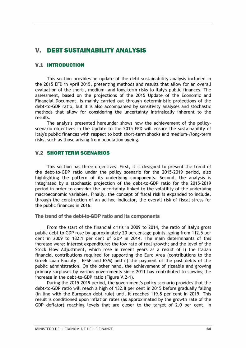
From the start of the financial crisis in 2009 to 2014, the ratio of Italy's gross

public debt to GDP rose by approximately 20 percentage points, going from 112.5 per

cent in 2009 to 132.1 per cent of GDP in 2014. The main determinants of this

increase were: interest expenditure; the low rate of real growth; and the level of the

Stock Flow Adjustment, which rose in recent years as a result of i) the Italian

financial contributions required for supporting the Euro Area (contributions to the

Greek Loan Facility , EFSF and ESM) and ii) the payment of the past debts of the

public administration. On the other hand, the achievement of sizeable and growing

primary surpluses by various governments since 2011 has contributed to slowing the

increase in the debt-to-GDP ratio (Figure V.2-1).

During the 2015-2019 period, the government's policy scenario provides that the

debt-to-GDP ratio will reach a high of 132.8 per cent in 2015 before gradually falling

(in line with the European debt rule) until it reaches 119.8 per cent in 2019. This

result is conditioned upon inflation rates (as approximated by the growth rate of the

GDP deflator) reaching levels that are closer to the target of 2.0 per cent. In

DRAFT BUDGETARY PLAN 2016 - DEBT SUSTAINABILITY ANALYSIS


addition, it is assumed that Italy's economy can return to gradually increasing levels

of real growth over the next four years. Finally, the debt reduction is to be

facilitated by a gradual decrease in the level of the Stock Flow Adjustment

attributable, first and foremost, to the disposal of public assets, with the

government counting on proceeds therefrom equivalent to approximately 1.5 per

cent of GDP in the 2016-2018 period. In any event, Figure V.2-1 illustrates that the

reduction of the debt-to-GDP ratio for the next few years is largely to be facilitated

by the maintenance of a sizeable primary surplus, averaging around 3.0 per cent of

GDP in the 2015-2019 period. Although relatively high, this average level is

nonetheless in line with the historical average of the pre-crisis years.

Figure V.2-1 Public debt determinants (% of GDP)

Stochastic simulations of the debt trend

In order to consider the uncertainty related to the macroeconomic forecasts

about the yield curve and about economic growth, the deterministic projection of

the debt-to-GDP ratio described above is integrated by several stochastic simulations

that incorporate both the historical volatility of short- and long-term interest rates

and the variability connected with nominal growth data43. For each year of the

projection and for each individual shock, it is possible to identify a distribution of the

debt-to-GDP ratio represented in probabilistic terms through a fan chart (Figures V.2-

2 and V.2-3).

43

Berti K., (2013), “Stochastic public debt projections using the historical variance-covariance matrix

approach for EU countries”, Economic Papers 480. The simulations were carried out with the Monte

Carlo method, using historical data for the yield curve and the nominal GDP growth rate, and applying

interest-rate and growth shocks to the trend of the debt-to-GDP ratio under the policy scenario. These

shocks were obtained by executing 2,000 extractions starting from a normal distribution with a zero

average and a variance-covariance matrix observed in the 1990-2014 period. More specifically, it is

assumed that the interest-rate shocks may be either temporary or permanent. In addition, it is assumed

that the temporary shocks to nominal growth will also wield their effects on the cyclical component of

the primary surplus.

DRAFT BUDGETARY PLAN 2016

66 MINISTERO DELL’ECONOMIA E DELLE FINANZE

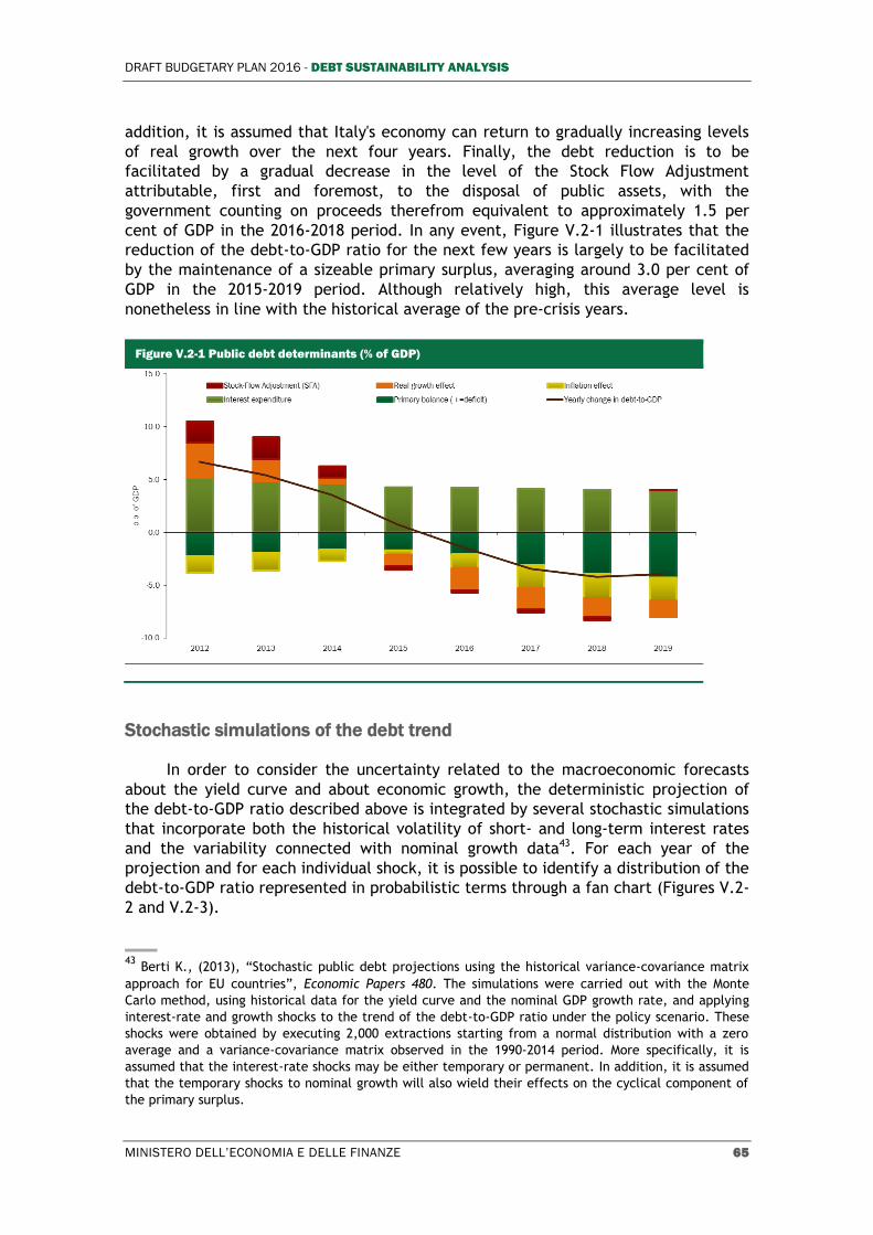
As shown by this analysis, under the effect of temporary and simultaneous

shocks to growth rates and interest rates (the range of which is calibrated to the past

volatility of these variables), the debt, in line with the government's projections, will

nonetheless continue to fall until it reaches a median value of approximately 120 per

cent of GDP in 2019. However, there is relatively high uncertainty recorded with

respect to the 2019 results, as shown by a difference of approximately 29 percentage

points between the tenth and ninetieth percentiles of the resulting debt distribution.

Figure V.2-2 Stochastic projection of the debt to GDP ratio with temporary shocks

Figure V.2-3 Stochastic projection of the debt to-GDP ratio with permanent shocks

Note: The graphs illustrate the tenth, twentieth, fortieth, fiftieth, sixtieth, eightieth and ninetieth percentiles of the

distribution of the debt-to-GDP ratio obtained with the stochastic simulation.

Source: MEF own calculations

In the event of a temporary shock, the trend of the debt-to-GDP ratio would

show a decrease for the first 40 percentiles as from 2015, between the fiftieth and

sixtieth percentiles as from 2016, and above the eightieth percentile as from 2017

only. In any event, even with the more severe shocks (which are found above the

eightieth percentile), the debt-to-GDP ratio would tend to stabilise after having

reached a peak of just around 140 per cent of GDP.

Instead, in the event of a permanent shock, the distribution of the values of

the debt-to-GDP ratio around the baseline scenario would be broader, but with a

debt trend that increases starting from the ninetieth percentile only.

Overall analysis of fiscal risks in the short term

This type of analysis is based on a series of variables, which, according to

empirical literature, have had a past role in forecasting risks to fiscal sustainability in

the short term. More specifically, 28 variables were considered, and clustered into

two sub-groups: fiscal and macro-financial variables. On the basis of the methodology

developed by the European Commission44, the analysis of the fiscal and macro-

financial variables allows for determining an indicator known as S0 that measures the

probability of the manifestation of a fiscal or financial crisis one year after.

The methodology underlying the calculation of the S0 indicator is linked to the

so-called signals-approach and allows for endogenously determining the thresholds,

for each of the variables included in the indicator, above which the probability of

crisis becomes more concrete. Any values of S0 or of the two sub-indices (fiscal and

44

Berti, K., Salto, M. and Lequien, M., (2012), ‘An early-detection index of fiscal stress for EU

countries’, European Economy Economic Papers n. 475.



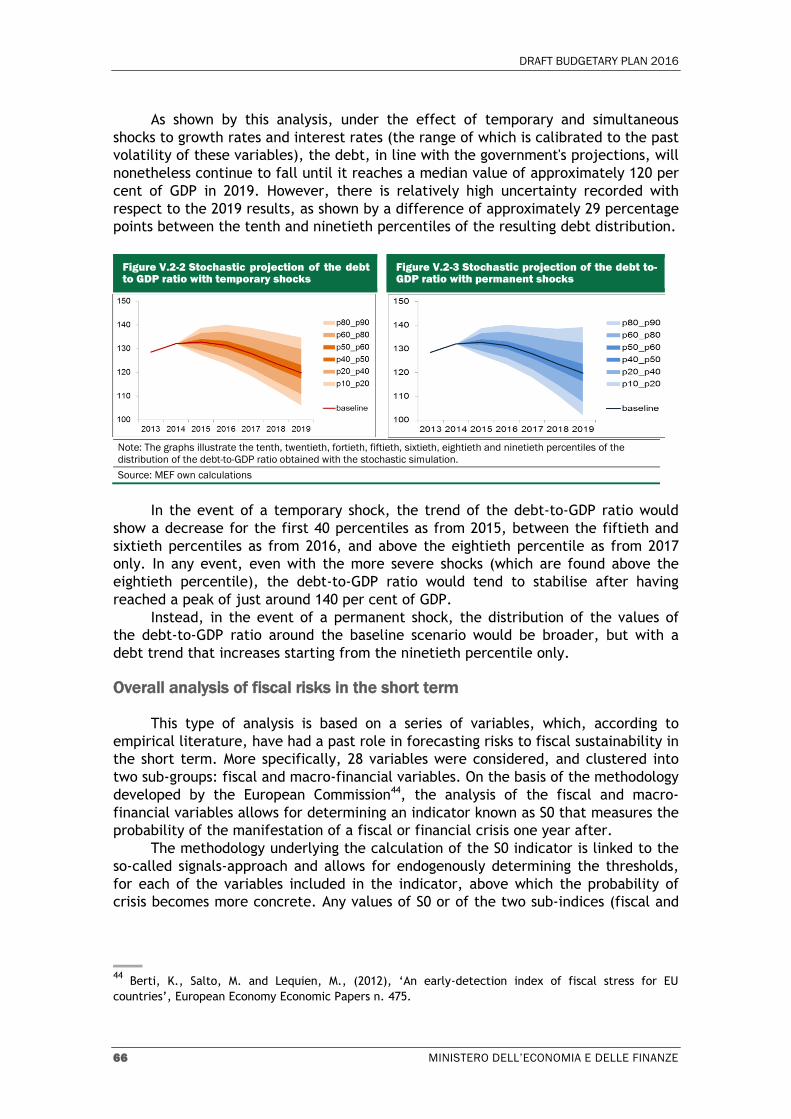
macro-financial) that might exceed their respective thresholds (0.43, 0.35 and 0.45)

are to be interpreted as signs of a growing risk in the short term.

As illustrated by Figure V.2-4, the overall risk in the short term has contracted

considerably since the peak in 2012. The improvement starting in 2013 affected both

sub-components, but was more pronounced for the fiscal sub-component. The S0

indicator stands around a value of 0.19, which is below the overall threshold (0.43).

The results for 2014 point to limited risk of fiscal crisis for the current year. The risk

of a fiscal crisis seems to be under control, as illustrated by the respective indicator

equal to 0.32, which is below the early warning benchmark (0.35). The probability of

a financial crisis is also below the levels that would raise concerns. The indicator

stands at 0.14 versus the respective benchmark of 0.45.

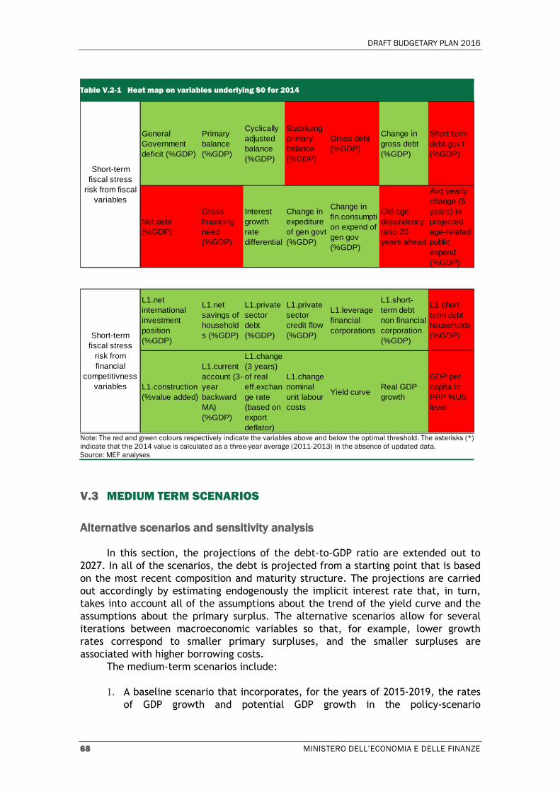
However, considering that the optimal thresholds are common to all of the

countries examined by the Commission, these values can only represent a preliminary

indicator about a country's sustainability in the short term. The punctual analysis

with respect to the individual variables that make up the S0 indicator shows that

several critical elements linked to the high level of the public debt could emerge in

the short term (in this regard, see the heat map presented in Table V.2-1)

Figure V.2-4 S0 indicator and sub-components

Note: For the years before 2014, the variables underlying the S0 are expressed in ESA 95.

Source: MEF analyses; AMECO; WEO and EUROSTAT

0.0

0.1

0.2

0.3

0.4

0.5

0.6

2011 2012 2013 2014

Fiscal index Financial competitiveness index Overall index S0



Table V.2-1 Heat map on variables underlying S0 for 2014

Note: The red and green colours respectively indicate the variables above and below the optimal threshold. The asterisks (*)

indicate that the 2014 value is calculated as a three-year average (2011-2013) in the absence of updated data.

Source: MEF analyses

V.3 MEDIUM TERM SCENARIOS

Alternative scenarios and sensitivity analysis

In this section, the projections of the debt-to-GDP ratio are extended out to

2027. In all of the scenarios, the debt is projected from a starting point that is based

on the most recent composition and maturity structure. The projections are carried

out accordingly by estimating endogenously the implicit interest rate that, in turn,

takes into account all of the assumptions about the trend of the yield curve and the

assumptions about the primary surplus. The alternative scenarios allow for several

iterations between macroeconomic variables so that, for example, lower growth

rates correspond to smaller primary surpluses, and the smaller surpluses are

associated with higher borrowing costs.

The medium-term scenarios include:

1. A baseline scenario that incorporates, for the years of 2015-2019, the rates

of GDP growth and potential GDP growth in the policy-scenario

General

Government

deficit (%GDP)

Primary

balance

(%GDP)

Cyclically

adjusted

balance

(%GDP)

Stabilizing

primary

balance

(%GDP)

Gross debt

(%GDP)

Change in

gross debt

(%GDP)

Short term

debt gov't

(%GDP)

Net debt

(%GDP)

Gross

financing

need

(%GDP)

Interest

growth

rate

differential

Change in

expediture

of gen govt

(%GDP)

Change in

fin.consumpti

on expend of

gen gov

(%GDP)

Old-age

dependency

ratio 20

years ahead

Avg yearly

change (5

years) in

projected

age-related

public

expend.

(%GDP)

1 1 0 0 0 1 1

0 0 0 0 0 0 1

L1.net

international

investment

position

(%GDP)

L1.net

savings of

household

s (%GDP)

L1.private

sector

debt

(%GDP)

L1.private

sector

credit flow

(%GDP)

L1.leverage

financial

corporations

L1.short-

term debt

non financial

corporation

(%GDP)

L1.short-

term debt

households

(%GDP)

L1.construction

(%value added)

L1.current

account (3-

year

backward

MA)

(%GDP)

L1.change

(3 years)

of real

eff.exchan

ge rate

(based on

export

deflator)

L1.change

nominal

unit labour

costs

Yield curve Real GDP

growth

GDP per

capita in

PPP %US

level

Short-term

fiscal stress

risk from fiscal

variables

Short-term

fiscal stress

risk from

financial

competitivness

variables



macroeconomic framework of the Update of the 2015 EFD. For the years

after 2019, the potential GDP growth rate is projected on the basis of a

production function model, in line with the methodology approved by the

EPC-Output Gap Working Group; such method assumes that the variables

related to the individual productive factors are extrapolated with simple

statistical techniques or they converge toward structural parameters (Table

V.3-1)45. The growth rate of the GDP deflator converges to 2.0 per cent as

from 2022. As from 2019, the structural primary balance is to be kept

constant at the reference level of 4.0 per cent of GDP until the end of the

forecast horizon. For the 2015-2019 period, the yield curve is that

underlying the Update to the EFD, whereas from January 2020, the yields

are kept constant at the values estimated for December 2019.

2. A pessimistic scenario that assumes GDP growth falls during the 2015-2019

period by 0.5 percentage points in each year with respect to the baseline

scenario. The potential GDP series for 2015-2019 is obtained by applying the

methodology agreed at a European level to the lower growth

macroeconomic framework. The output gap is closed as of 2022, while the

NAWRU and Total Factor Productivity (TFP) converge in 2027 to the average

values for the crisis period (2011-2013). The yield curve is equivalent to

that in the baseline scenario with an increase of 100 basis points starting

from 2016 and through 2018. The trend in interest rates between late April

2015 and July 2015 suggests that, despite the QE, the worsening of the

perception of credit risk may affect the yield curve as well as the spread

against German bonds. In 2019, the shock is reduced to 50 basis points,

whereas the yields thereafter are assumed to converge toward the value in

the baseline scenario.

3. An optimistic scenario that assumes GDP growth rises during the 2015-2018

period by 0.5 percentage points in each year with respect to the baseline

scenario. The potential GDP series for 2015-2018 is obtained by applying the

methodology agreed at a European level to the higher growth

macroeconomic framework. The output gap is closed as of 2022, while the

NAWRU and Total Factor Productivity (TFP) converge in 2027 to the pre-

crisis averages. The yield curve is equivalent to that in the baseline

scenario with a decrease of 50 basis points starting from 2017 to 2019. In

the final years of the projection, the yields are assumed to be constant at

the level of the baseline scenario.

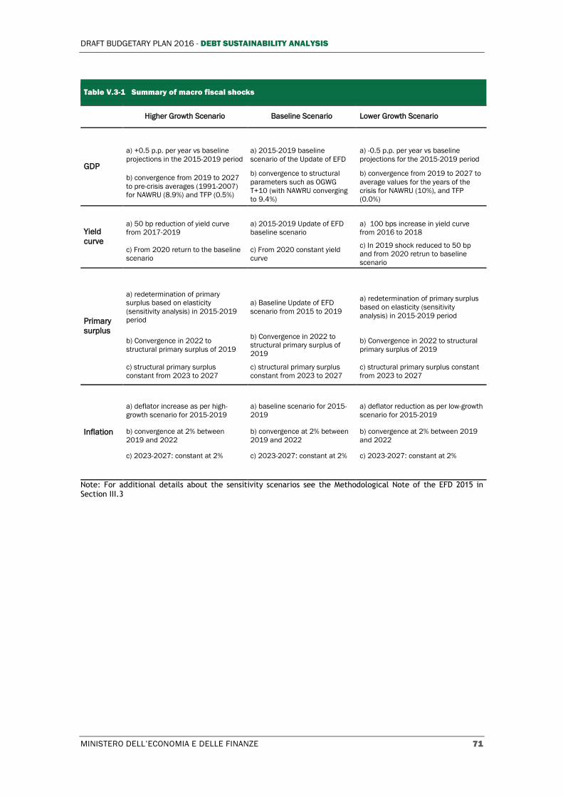
Table V.3-1 illustrates more specifically the characteristics of the shocks

applied to the principal macroeconomic and public-finance variables underlying the

trend of the debt-to-GDP ratio. Table V.3-2 reports the values of the main

macroeconomic and public-finance variables in the different scenarios for the 2015-

2019 period as well as the values of convergence at the end of the medium-term

projection horizon.

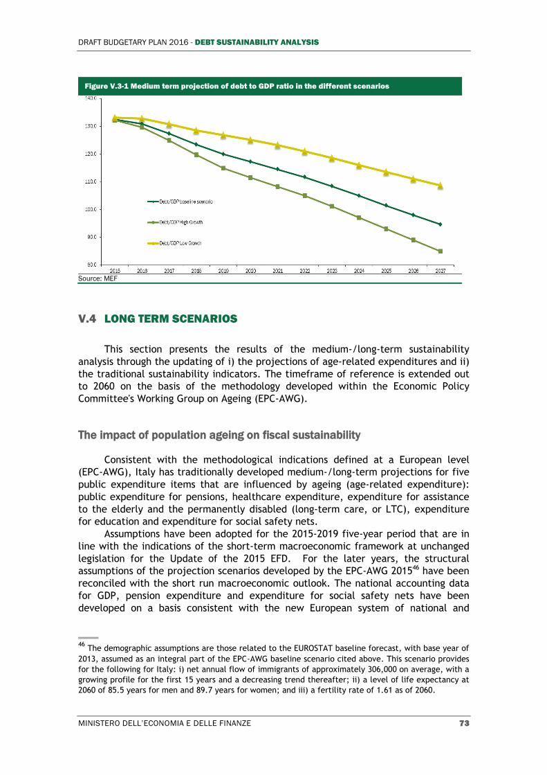
On the basis of the macroeconomic and public-finance assumptions considered,

Figure V.3-1 confirms the declining medium-term trend of the debt-to-GDP ratio in

all of the scenarios.

45

For additional details about the methods for convergence to the structural values, see the

Methodological Note of the 2015 EFD in Section III.3.



Though starting at a level above 130 per cent, the debt-to-GDP ratio in the

higher growth scenario would fall rapidly to reach 78.5 per cent in 2027,

approximately 15 percentage points below the figure for the baseline scenario.

Instead, the debt-to-GDP ratio in the lower growth scenario would decline, but would

reach a value of 115.6 per cent in 2027, approximately 23 percentage points above

the figure for the baseline scenario.

The debt rule calculated based on the forward-looking criterion would be

respected in 2016 under both the baseline scenario and the optimistic scenario.

When calculated on the basis of the backward-looking criterion, the rule would be

respected as from 2018 in the high-growth scenario and as from 2024 in the baseline

scenario. Instead, in the case of lower growth, the debt-to-GDP ratio would not fall

in accordance with the provisions of the debt rule, and would remain above the

benchmark for the entire period of the simulation.



Table V.3-1 Summary of macro fiscal shocks

Higher Growth Scenario Baseline Scenario Lower Growth Scenario

GDP

a) +0.5 p.p. per year vs baseline

projections in the 2015-2019 period

a) 2015-2019 baseline

scenario of the Update of EFD

a) -0.5 p.p. per year vs baseline

projections for the 2015-2019 period

b) convergence from 2019 to 2027

to pre-crisis averages (1991-2007)

for NAWRU (8.9%) and TFP (0.5%)

b) convergence to structural

parameters such as OGWG

T+10 (with NAWRU converging

to 9.4%)

b) convergence from 2019 to 2027 to

average values for the years of the

crisis for NAWRU (10%), and TFP

(0.0%)

Yield

curve

a) 50 bp reduction of yield curve

from 2017-2019

a) 2015-2019 Update of EFD

baseline scenario

a) 100 bps increase in yield curve

from 2016 to 2018

c) From 2020 return to the baseline

scenario

c) From 2020 constant yield

curve

c) In 2019 shock reduced to 50 bp

and from 2020 retrun to baseline

scenario

Primary

surplus

a) redetermination of primary

surplus based on elasticity

(sensitivity analysis) in 2015-2019

period

a) Baseline Update of EFD

scenario from 2015 to 2019

a) redetermination of primary surplus

based on elasticity (sensitivity

analysis) in 2015-2019 period

b) Convergence in 2022 to

structural primary surplus of 2019

b) Convergence in 2022 to

structural primary surplus of

2019

b) Convergence in 2022 to structural

primary surplus of 2019

c) structural primary surplus

constant from 2023 to 2027

c) structural primary surplus

constant from 2023 to 2027

c) structural primary surplus constant

from 2023 to 2027

Inflation

a) deflator increase as per high-

growth scenario for 2015-2019

a) baseline scenario for 2015-

2019

a) deflator reduction as per low-growth

scenario for 2015-2019

b) convergence at 2% between

2019 and 2022

b) convergence at 2% between

2019 and 2022

b) convergence at 2% between 2019

and 2022

c) 2023-2027: constant at 2% c) 2023-2027: constant at 2% c) 2023-2027: constant at 2%

Note: For additional details about the sensitivity scenarios see the Methodological Note of the EFD 2015 in Section III.3



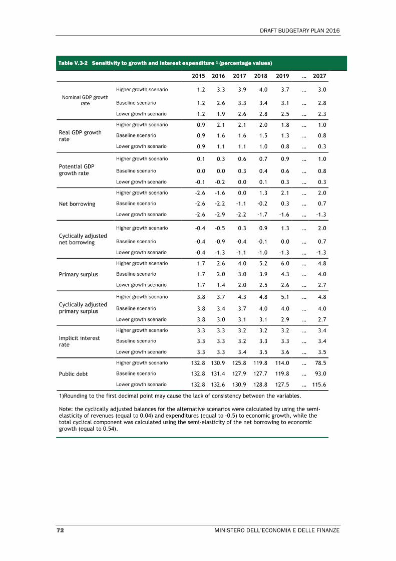
Table V.3-2 Sensitivity to growth and interest expenditure 1 (percentage values)

2015 2016 2017 2018 2019 … 2027

Nominal GDP growth

rate

Higher growth scenario 1.2 3.3 3.9 4.0 3.7 … 3.0

Baseline scenario 1.2 2.6 3.3 3.4 3.1 … 2.8

Lower growth scenario 1.2 1.9 2.6 2.8 2.5 … 2.3

Real GDP growth rate




Potential GDP growth rate



Lower growth scenario -0.1 -0.2 0.0 0.1 0.3 … 0.3

Net borrowing

Higher growth scenario -2.6 -1.6 0.0 1.3 2.1 … 2.0

Baseline scenario -2.6 -2.2 -1.1 -0.2 0.3 … 0.7

Lower growth scenario -2.6 -2.9 -2.2 -1.7 -1.6 … -1.3

Cyclically adjusted net borrowing

Higher growth scenario -0.4 -0.5 0.3 0.9 1.3 … 2.0

Baseline scenario -0.4 -0.9 -0.4 -0.1 0.0 … 0.7

Lower growth scenario -0.4 -1.3 -1.1 -1.0 -1.3 … -1.3

Primary surplus




Cyclically adjusted primary surplus




Implicit interest rate




Public debt




1)Rounding to the first decimal point may cause the lack of consistency between the variables.

Note: the cyclically adjusted balances for the alternative scenarios were calculated by using the semi-elasticity of revenues (equal to 0.04) and expenditures (equal to -0.5) to economic growth, while the total cyclical component was calculated using the semi-elasticity of the net borrowing to economic growth (equal to 0.54).



Figure V.3-1 Medium term projection of debt to GDP ratio in the different scenarios

Source: MEF

V.4 LONG TERM SCENARIOS

This section presents the results of the medium-/long-term sustainability

analysis through the updating of i) the projections of age-related expenditures and ii)

the traditional sustainability indicators. The timeframe of reference is extended out

to 2060 on the basis of the methodology developed within the Economic Policy

Committee's Working Group on Ageing (EPC-AWG).

The impact of population ageing on fiscal sustainability

Consistent with the methodological indications defined at a European level

(EPC-AWG), Italy has traditionally developed medium-/long-term projections for five

public expenditure items that are influenced by ageing (age-related expenditure):

public expenditure for pensions, healthcare expenditure, expenditure for assistance

to the elderly and the permanently disabled (long-term care, or LTC), expenditure

for education and expenditure for social safety nets.

Assumptions have been adopted for the 2015-2019 five-year period that are in

line with the indications of the short-term macroeconomic framework at unchanged

legislation for the Update of the 2015 EFD. For the later years, the structural

assumptions of the projection scenarios developed by the EPC-AWG 201546 have been

reconciled with the short run macroeconomic outlook. The national accounting data

for GDP, pension expenditure and expenditure for social safety nets have been

developed on a basis consistent with the new European system of national and

46

The demographic assumptions are those related to the EUROSTAT baseline forecast, with base year of

2013, assumed as an integral part of the EPC-AWG baseline scenario cited above. This scenario provides

for the following for Italy: i) net annual flow of immigrants of approximately 306,000 on average, with a

growing profile for the first 15 years and a decreasing trend thereafter; ii) a level of life expectancy at

2060 of 85.5 years for men and 89.7 years for women; and iii) a fertility rate of 1.61 as of 2060.



regional accounts (ESA 2010). The projections for the 2015-2019 period are in line

with those underlying the public-finance framework of the 2015 Update of the EFD.

The projection of pension expenditure incorporates the effects of Decree-Law

No. 65/2015, converted with Law No. 109/2015, and namely, the provision that

implements the principles of the Constitutional Court Ruling No. 70/2015 regarding

the unconstitutionality of de-indexing payments for pensions exceeding three times

the minimum.

Overall, the ratio of age-related expenditure to GDP is stable for the 2015-2060

period, and averages around 27.8 per cent of GDP. However, in the years after 2015,

the expenditure falls slightly before starting to rise again as of 2030, and reaching

28.5 per cent of GDP around 2042. The aggregate age-related expenditure falls in the

final years of the forecast, amounting to 27 per cent of GDP in 2060.

With reference to the individual components, the ratio of pension expenditure,

which rose during the crisis due exclusively to the decrease in level of nominal GDP,

is projected to decrease as of 2015, due to the effects of the reform introduced with

Law No. 214/2011. Starting from a level of 15.8 per cent of GDP, the pension

expenditure declines to 15.3 per cent in 2020. In the later years, with the impact of

the retirement of the Baby Boom generation, the ratio starts growing again to reach

a high of 15.9 per cent of GDP in 2040. During the final years of the projection

horizon, the ratio of pension expenditure to GDP falls rapidly to reach around 13.8

per cent in 2060.

The projection of healthcare expenditure is carried out on the basis of the so-

called reference scenario methodology, which incorporates both age-related effects

as well as the effects of additional explicative factors capable of significantly

influencing the trend of healthcare expenditure. It follows that the projections of

the ratio of healthcare expenditure to GDP initially declines for the effect of the

cost-containment measures recently legislated, and it then starts to grow as from

2020 to amount to approximately 7.6 per cent in the final 10 years of the forecast

period.

The expenditure for assistance to the elderly and permanently disabled is

initially stable in relation to GDP. Subsequently it grows constantly reaching 1.6 per

cent of GDP in 2060.

The projection expenditure for social safety nets in relation to GDP goes from

1.0 per cent in 2015, and then gradually decreases to around 0.6 per cent as from

2030.

Finally, the projection expenditure for education in relation to GDP presents a

gradual reduction for the 2015-2033 period, going from an initial level of 3.7 per cent

to 3.3 per cent of GDP. In the later years, expenditure is projected to grow to reach

around 3.5 per cent of GDP in 2060.

Fiscal sustainability indicators

The medium- and long-term indicators (S1 and S2) allow to assess the impact of

implicit age-related liabilities on fiscal sustainability over the medium/long term.

The medium-term sustainability indicator (S1) shows the increase in the

structural primary balance to be achieved cumulatively in the years 2019 and 2020 so

as to ensure, if the increase is maintained constant thereafter, both the achievement

of a debt-to-GDP ratio of 60 per cent by 2030 and to offset the age-related costs.

The long-term sustainability indicator (S2) shows the fiscal adjustment in terms of

structural primary balance which, if immediately realized and maintained, allows for



complying with the intertemporal budget constraint from 2019 and over an infinite

time horizon.

Both indicators are based on the growth projections and fiscal targets outlined

in the policy scenario in the 2015 Update of the EFD, and incorporate the medium-

/long-term projections of age-related expenditures. The higher and more positive

the values of the S1 and S2 sustainability indicators, the greater will be the need for

fiscal adjustment and thus, the greater the sustainability risk will be. Other

conditions being equal, higher projected age-related expenditures will make the

compliance with the intertemporal budget constraint harder as higher primary

surpluses will be required.

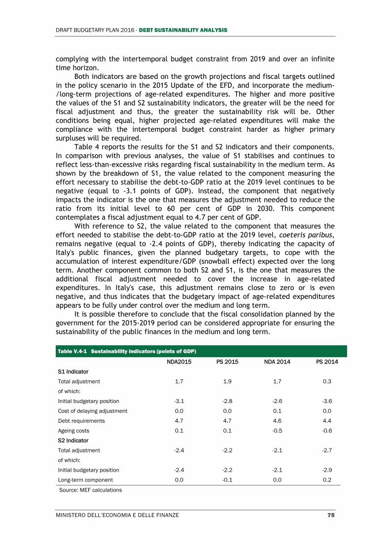
Table 4 reports the results for the S1 and S2 indicators and their components.

In comparison with previous analyses, the value of S1 stabilises and continues to

reflect less-than-excessive risks regarding fiscal sustainability in the medium term. As

shown by the breakdown of S1, the value related to the component measuring the

effort necessary to stabilise the debt-to-GDP ratio at the 2019 level continues to be

negative (equal to -3.1 points of GDP). Instead, the component that negatively

impacts the indicator is the one that measures the adjustment needed to reduce the

ratio from its initial level to 60 per cent of GDP in 2030. This component

contemplates a fiscal adjustment equal to 4.7 per cent of GDP.

With reference to S2, the value related to the component that measures the

effort needed to stabilise the debt-to-GDP ratio at the 2019 level, coeteris paribus,

remains negative (equal to -2.4 points of GDP), thereby indicating the capacity of

Italy's public finances, given the planned budgetary targets, to cope with the

accumulation of interest expenditure/GDP (snowball effect) expected over the long

term. Another component common to both S2 and S1, is the one that measures the

additional fiscal adjustment needed to cover the increase in age-related

expenditures. In Italy's case, this adjustment remains close to zero or is even

negative, and thus indicates that the budgetary impact of age-related expenditures

appears to be fully under control over the medium and long term.

It is possible therefore to conclude that the fiscal consolidation planned by the

government for the 2015-2019 period can be considered appropriate for ensuring the

sustainability of the public finances in the medium and long term.

Table V.4-1 Sustainability indicators (points of GDP)

NDA2015 PS 2015 NDA 2014 PS 2014

S1 Indicator

Total adjustment 1.7 1.9 1.7 0.3

of which:

Initial budgetary position -3.1 -2.8 -2.6 -3.6

Cost of delaying adjustment 0.0 0.0 0.1 0.0

Debt requirements 4.7 4.7 4.6 4.4

Ageing costs 0.1 0.1 -0.5 -0.6

S2 Indicator

Total adjustment -2.4 -2.2 -2.1 -2.7

of which:

Initial budgetary position -2.4 -2.2 -2.1 -2.9

Long-term component 0.0 -0.1 0.0 0.2

Source: MEF calculations



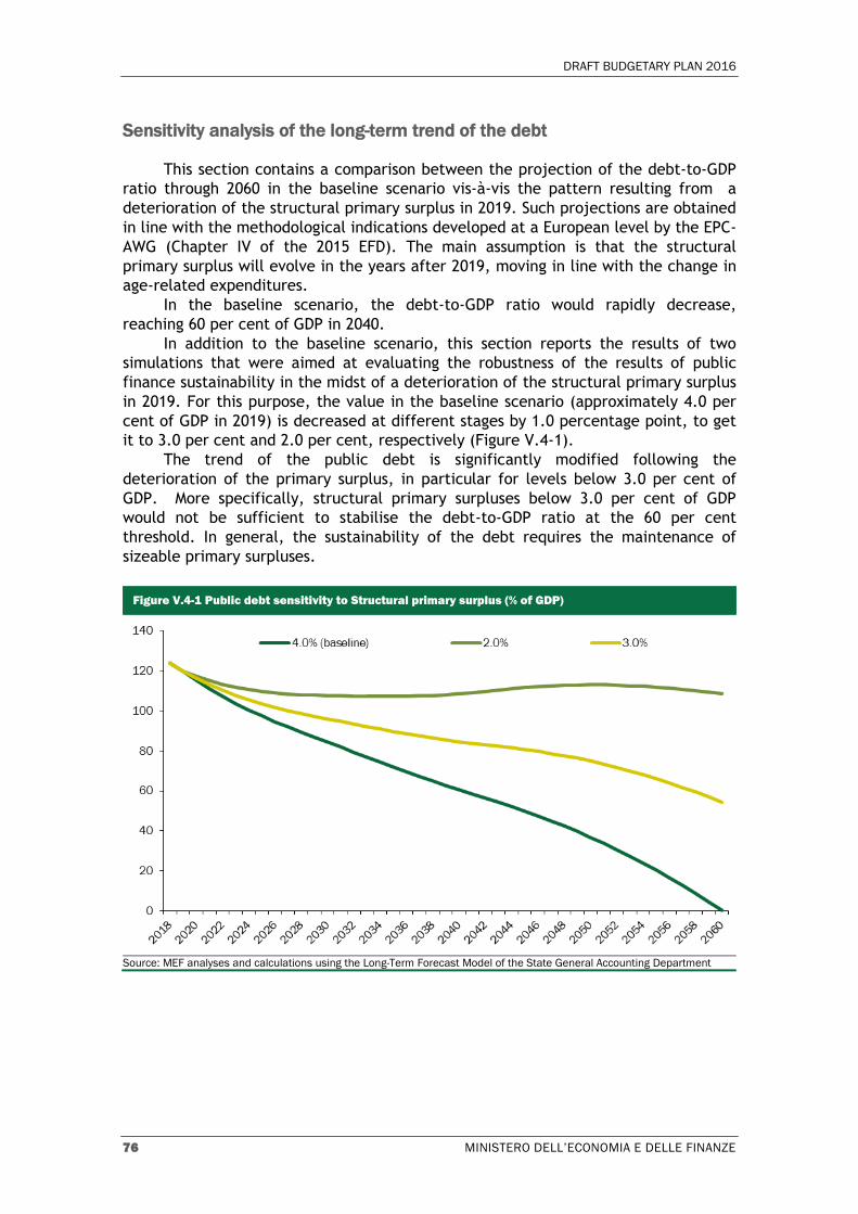
Sensitivity analysis of the long-term trend of the debt

This section contains a comparison between the projection of the debt-to-GDP

ratio through 2060 in the baseline scenario vis-à-vis the pattern resulting from a

deterioration of the structural primary surplus in 2019. Such projections are obtained

in line with the methodological indications developed at a European level by the EPC-

AWG (Chapter IV of the 2015 EFD). The main assumption is that the structural

primary surplus will evolve in the years after 2019, moving in line with the change in

age-related expenditures.

In the baseline scenario, the debt-to-GDP ratio would rapidly decrease,

reaching 60 per cent of GDP in 2040.

In addition to the baseline scenario, this section reports the results of two

simulations that were aimed at evaluating the robustness of the results of public

finance sustainability in the midst of a deterioration of the structural primary surplus

in 2019. For this purpose, the value in the baseline scenario (approximately 4.0 per

cent of GDP in 2019) is decreased at different stages by 1.0 percentage point, to get

it to 3.0 per cent and 2.0 per cent, respectively (Figure V.4-1).

The trend of the public debt is significantly modified following the

deterioration of the primary surplus, in particular for levels below 3.0 per cent of

GDP. More specifically, structural primary surpluses below 3.0 per cent of GDP

would not be sufficient to stabilise the debt-to-GDP ratio at the 60 per cent

threshold. In general, the sustainability of the debt requires the maintenance of

sizeable primary surpluses.

Figure V.4-1 Public debt sensitivity to Structural primary surplus (% of GDP)

Source: MEF analyses and calculations using the Long-Term Forecast Model of the State General Accounting Department



Simulations with respect to pension reforms

As shown by the sensitivity tests presented in the preceding section, when

based on the government's budget objectives outlined in the Update to 2015 EFD

(namely, the achievement of the Medium-Term Objective in 2018 and its

maintenance in the years thereafter), the long-term trend of age-related

expenditure would not jeopardise the sustainability of the Italy's public debt, even in

the presence of particularly adverse macroeconomic, demographic or fiscal

conditions. It should nonetheless be pointed out that this conclusion is the by-

product of intensive pension reforms that have significantly contributed to reducing

age-related expenditure over the past 20 years.

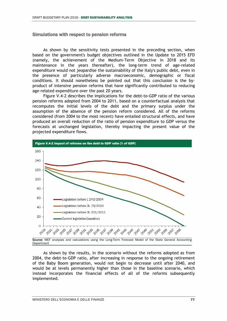
Figure V.4-2 describes the implications for the debt-to-GDP ratio of the various

pension reforms adopted from 2004 to 2011, based on a counterfactual analysis that

recomputes the initial levels of the debt and the primary surplus under the

assumption of the absence of the pension reform considered. All of the reforms

considered (from 2004 to the most recent) have entailed structural effects, and have

produced an overall reduction of the ratio of pension expenditure to GDP versus the

forecasts at unchanged legislation, thereby impacting the present value of the

projected expenditure flows.

Figure V.4-2 Impact of reforms on the debt to GDP ratio (% of GDP)

Source: MEF analyses and calculations using the Long-Term Forecast Model of the State General Accounting Department

As shown by the results, in the scenario without the reforms adopted as from

2004, the debt-to-GDP ratio, after increasing in response to the ongoing retirement

of the Baby Boom generation, would not begin to decrease until after 2040, and

would be at levels permanently higher than those in the baseline scenario, which

instead incorporates the financial effects of all of the reforms subsequently

implemented.

v. debt sustainability analysis. debt sustainability analysis ... integrated by a stochastic...

Documents