native forest strategic yield scheduling
TRANSCRIPT

N S W W E S T E R N R E G I O N A L A S S E S S M E N T S
Nandewar
Native ForestStrategic Yield
Scheduling
N A N D 0 8 ( V o l 7 )December 2003
R E S O U R C E A N D C O N S E R V A T I O N A S S E S S M E N T C O U N C I L
N S W W E S T E R N R E G I O N A L A S S E S S M E N T S
Nandewar
Native Forest
Strategic Yield Scheduling
John Turland
State Forests of NSW
NAND08
R E S O U R C E A N D C O N S E R V A T I O N A S S E S S M E N T C O U N C I L

I N F O R M AT I O N
Crown Copyright December 2003
NSW Government
ISBN: 1 74029 221 9
This project has been funded and coordinated by the Resourceand Conservation Division (RACD) of the NSW Department ofInfrastructure, Planning and Natural Resources, for the Resourceand Conservation Assessment Council (RACAC)
Preferred way to cite this publication:
Turland, J. 2003 Native Forest Strategic Yield Scheduling. Nandewar Bio-Region. NSW WesternRegional Assessments. Project Number: NAND 08. Resource and Conservation Assessment Council.48p.p
For more information and for information on access to data, contact:
Resource and Conservation Division, Department of Infrastructure, Planning and Natural Resources
P.O. Box 39
SYDNEY NSW 2001
Phone: 02 9228 6586
Fax: 02 9228 6411
Email: [email protected]
Author:
John Turland
State Forests of NSW
Disclaimer
While every reasonable effort has been made to ensure that this document is correct at the time ofprinting, the State of New South Wales, its agents and employees, do not assume any responsibility andshall have no liability, consequential or otherwise, of any kind, arising from the use of or reliance on anyof the information contained in this document.

N SW W EST ER N R EG IO N AL A SS ES S MEN T S – N AN D EW AR
NATIVE FOREST STRATEGIC YIELD SCHEDULING
Contents
Project Summary I
Acronyms and abbreviations II
Glossary III
i 1Introduction 1
1 2Harvest Scheduling 2
1.1 GENERAL BACKGROUND ON HARVEST SCHEDULING 2
1.2 OVERVIEW OF MODELLING APPROACH AND METHODOLOGY 4
2 7Area Database 7
2.1 AREA DEFINITION 7
2.1.1 Forest Management Zones 9
2.1.2 Exclusions 10
2.1.3 Net Harvest Area Modifier 11
2.2 LAND ATTRIBUTES 12
2.2.1 Timber Supply Zone 12
2.2.2 Timber Price Zone 13
2.2.3 Silvicultural Forest Types 13
2.3.4 Stratification 14
2.3 WOODSTOCK AREA FILE STRUCTURE AND FORMAT 17
3 19Yield Table File 19
3.1 WOODSTOCK YIELD TABLE STRUCTURE AND FORMAT 19
3.2 EXPLANATION OF STRATA-LEVEL TIME-DEPENDENT YIELD TABLES 23

N SW W EST ER N R EG IO N AL A SS ES S MEN T S – N AN D EW AR
3.3 YIELD TABLE OPTIONS FOR REGULATING HARVEST YIELDS 25
3.4 STRATEGIC NOT OPERATIONAL LEVEL YIELD FORECASTS 27
3.5 SILVICULTURAL PRESCRIPTIONS 28
3.6 LOG SPECIFICATIONS AND GRADES 30
4 31Woodstock Model Template Structure 31
4.1 CONTROL SECTION 31
4.2 LIFESPAN SECTION 32
4.3 AGGREGATE SECTION 32
4.4 ACTIONS SECTION 33
4.5 TRANSITIONS SECTION 34
4.6 OPTIMIZE SECTION 35
4.7 OUTPUTS SECTION 36
4.8 REPORTS SECTION 38
4.9 SCHEDULE SECTION 38
4.10 GRAPHICS SECTION 39
5 40Wood Supply Forecasting 40
5.1 MANAGEMENT OBJECTIVES AND CONSTRAINTS 40
5.2 MODELLING APPROACH 42
6 43Base Case Wood Supply Forecast 43
6.1 SCENARIO 43
6.2 RESULTS 44
7 48References 48

NATIVE FOREST STRATEGIC YIELD SCHEDULING
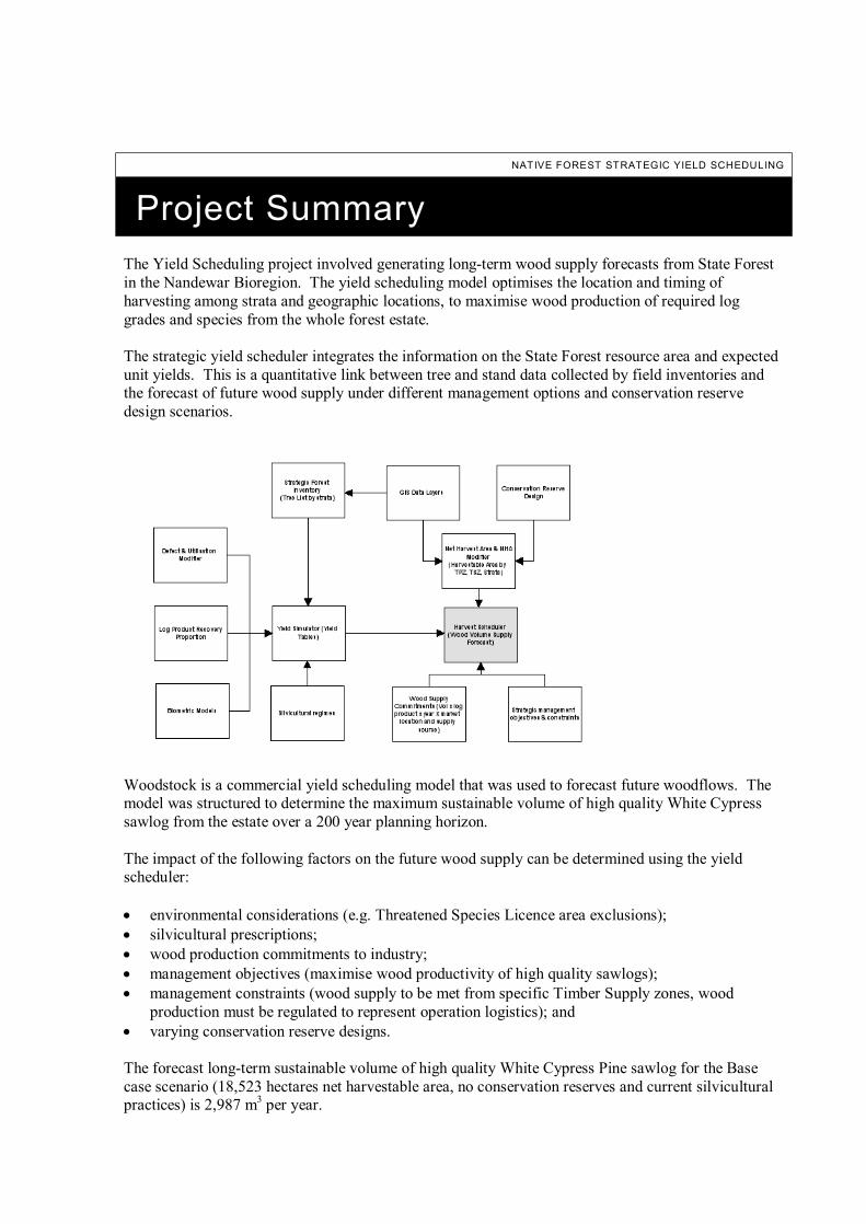
Project SummaryThe Yield Scheduling project involved generating long-term wood supply forecasts from State Forestin the Nandewar Bioregion. The yield scheduling model optimises the location and timing ofharvesting among strata and geographic locations, to maximise wood production of required loggrades and species from the whole forest estate.
The strategic yield scheduler integrates the information on the State Forest resource area and expectedunit yields. This is a quantitative link between tree and stand data collected by field inventories andthe forecast of future wood supply under different management options and conservation reservedesign scenarios.
Woodstock is a commercial yield scheduling model that was used to forecast future woodflows. Themodel was structured to determine the maximum sustainable volume of high quality White Cypresssawlog from the estate over a 200 year planning horizon.
The impact of the following factors on the future wood supply can be determined using the yieldscheduler:
• environmental considerations (e.g. Threatened Species Licence area exclusions);• silvicultural prescriptions;• wood production commitments to industry;• management objectives (maximise wood productivity of high quality sawlogs);• management constraints (wood supply to be met from specific Timber Supply zones, wood
production must be regulated to represent operation logistics); and• varying conservation reserve designs.
The forecast long-term sustainable volume of high quality White Cypress Pine sawlog for the Basecase scenario (18,523 hectares net harvestable area, no conservation reserves and current silviculturalpractices) is 2,987 m3 per year.

II N SW W EST ER N R EG IO N AL A SS ES S MEN T S – N AN D EW AR
NATIVE FOREST STRATEGIC YIELD SCHEDULING
Acronyms and abbreviationsBA- Basal Area (m2/ha)
FMZ - Forest Management Zone
GS –Growing Stock
HQ –High Quality
LP – Linear Programming
NCT – Non-commercial Thinning
IBK – Ironbark species
WCP – White Cypress Pine
MIX – Mixed Speceis
TPZ – Timber Price Zone
TSL – Threatened Species Licence
TSZ - Timber Supply Zone
Vol – Volume (m3/ha)
NATIVE FOREST STRATEGIC YIELD SCHEDULING
Glossary
Age dependent yields - yields are expressed as recoverable volume (m3/ha) or weight (tonnes/ha) oflog products, which will be harvested by age.
Analysis unit - aspatial units of land used for strategic level yield scheduling. This is the total area ofland with unique combinations of strata and geographic area units (Management Area,Forest, Timber Price Zone and Timber Supply Zone). These may be non-contiguousblocks of land. Each analysis unit is the basic unit of area in the strategic schedulingmodel and is assigned the same management options. The yield scheduler may elect toapply different subsets of the options to subsets of the analysis unit.
Commercial thinning - a harvesting operation which involves the removal of a portion of thestanding forest for the production of merchantable logs. The aim of harvesting is toproduce saleable logs, but only a portion of the stand is removed in thinning. The intent isto open up a stand as it approaches or is enduring strong competition for resources (light,space, nutrients and, water) for one or more reasons. If stand growth was stagnating theremoval of some trees enables: the remaining trees to reach larger more desirablediameters; the stimulation of regeneration of shade intolerant species; the retention ofsome trees for seed and possibly as a nurse crop; and the release of stagnant advancegrowth.
Growing Stock – term for the standing forest. In forest that is selectively harvested, this is the portionof a stand retained after a harvesting operation.
Forest Type – forest characterised by a unique blend of tree species or genera. The floristiccomposition may vary significantly, but will be characterised by an identified dominanceof one or more species. The canopy tree species and understorey vegetation may also beused to define the forest type.
Harvest Scheduling – the application of techniques (computer models) to determine the schedule ofharvesting of forest areas to achieve a wood supply target; the process of determining theallowable cut/sustainable yield over multiple rotations or cutting cycles
Management Area – The primary subdivision of a forest region into broad geographically discreteand contiguous units that are convenient areas for forest management purposes.
Net Harvestable Area – the forest area remaining after deducting mappable exclusion areas from thegross area.

IV N SW W EST ER N R EG IO N AL A SS ES S MEN T S – N AN D EW AR
Net Harvestable Area Modifier – a ratio that is used to reduce the eligible net harvest area to actualharvest area due to unmapped and unmappable factors.
Non – commercial thinning – a harvesting operation that involves the removal of a portion of thestanding forest. The operation removes excess numbers of undesirable (usually non-commercial or unmerchantable quality trees depending on regulations) and/or smalldiameter trees (too many to achieve future crop of desirable size trees). Trees are retainedin even spacings to achieve maximum site utilisation and individual tree growth. The aimis to open up a stand as it approaches or is enduring strong competition for resources(light, space, nutrients and water), or to unlock stagnant stands, enabling the remainingand more desirable trees to reach larger more preferable diameters. No commercialmerchantable quality logs are recovered from these operations. The primary aim of Non-commercial thinning is to improve the stand whereby future yields will be improved.
Overstorey – In a multi-aged forest, this is the upper most tier forming the canopy of the stand andcomprises the older most mature trees. This component of the stand is harvested forsawlog production.
Planning Unit - spatial land units (polygon) in a GIS layer with unique combinations of compartment,Flora Reserve, Timber Supply zone, Timber Price Zone and Forest Types. These areamalgamations of spatial analysis units. These are discrete units of land that are used inthe Conservation Reserve design.
Recoverable Yield – the yield actually harvested and removed form the forest. This equates to theassessed merchantable volume less reductions for internal defect, breakage & degradeduring harvesting, variations in cross cutting and errors in volume formulae etc.
Release operation – a harvesting operation where all commercial species of overstorey trees ofmerchantable size and quality are removed from a stand to release the regeneration oradvanced regeneration cohorts.
Silvicultural Regime - a sequence of forestry operations used to manage a forest stand to achieve adesired range of wood products over time and maintain other non-wood values for socialand environmental purposes. The operations in native forests may include standtreatments to improve stand tree quality and forest health (non-commercial thinning, TSI),harvesting operations removing timber (commercial thinning, releasing) and hazardreduction (e.g. low intensity burns). Harvesting operations may be selective, group, orcoupe based removal. Enrichment planting may be adopted where insufficient naturalregeneration occurs. The regime is defined from initial site preparation and regenerationto the stand endpoint when the regeneration cohort has matured and harvested (orbecomes a habitat tree)
Spatial Analysis Unit – unique spatial land units (polygon) in a GIS layer in which all spatial landattributes have been combined. These are unique intersections of Compartment, FloraReserve, FMZ, 4x Stream order buffers, road buffers (area occupied by roads), Slopes<>10 deg, Forest Types, Timber Supply zone and Timber Price Zone.
Species – botanical classification of plants with unique characteristics. Individual tree species aremodelled in the growth and yield simulator, though various growth models are assigned tobroad species groups, which are not necessarily closely related botanically, but exhibitsimilar trends and rates of growth.
Stand – a generic term used for describing or referring to a discrete but small area of trees. A standcan be a geographic mapped subdivision of a compartment/planning unit that is theprimary subdivision of a forest defining trees being managed uniformly. The stand maybe single or mixed species and may be even-aged or multi-aged. Within a forest, a clumpof trees exhibiting similar characteristics in terms of specie or species mix and age orstructure may be referred to as a stand. The defining feature is that a stand is a discreteunit characterised by a uniform feature or uniform silvicultural management.
Stratification – the process of delineating unique forest areas and creating strata.
Stratum - a grouping of forest land units according to one or more similar characteristics, such asspecies, forest type, stand structure, silviculture, management history, productivity, slope,and distance from market. Alternatively defined, it is a subdivision of a population intohomogenous units depending on the objectives (e.g. static inventory, growth & yieldmodelling, operation planning). The aim is to create units that are more homogenous thanthe whole population, and therefore more representative and precise information can bedetermined about that unit of forest.
Timber Price Zone - geographically contiguous areas with similar log royalty structures based ontimber species groups, harvesting terrain and haulage distance to markets. The TimberPrice Zones provide a useful geographical basis for reporting the source of wood whenevaluating wood supply options.
Timber Supply Zone - small groups of compartments within a Timber Catchment that have similartimber resource characteristics and silvicultural requirements. These are logical self-contained timber management units in terms of infrastructure and geographicalboundaries. The Timber Supply Zones provide a good geographical basis for reportingthe options’ source of wood when evaluating wood supply options.
Time dependent yields - yields are expressed as recoverable volume (m3/ha) or weight (tonnes/ha)of log products which will be harvested by year (or period).
Wood supply forecast – a forecast of the expected future wood supply from a defined forest area overa planning horizon. A forecast may quantify the expected volume or tonnage or logs ofdifferent species and log grades from identifiable geographic areas an/or forest classes(stratum, forest type).
Woodstock – A commercial yield scheduling computer model.

VI N SW W EST ER N R EG IO N AL A SS ES S MEN T S – N AN D EW AR
Yield – the quantity of merchantable wood products removed from a forest in a harvesting operation.High quality/value log products are usually defined in terms of volume (e.g. m3) and lowerquality/value products such as pulpwood or firewood are defined in terms of weight (e.g.tonnes).
Yield table – is a tabular statement of forecasted quantity of products (potential unit yields) that canbe harvested from a forest area over time when managed under a particular silviculturalregime, expressed in terms of volume or weight per hectare. Several forms of yield tableexist – age dependent and time-dependent. In plantations yield is usually expressed as afunction of age showing expected yields from commercial thinning, but showing thepotential yield from clearfelling at a range of potential rotation ages. In multi-aged forestyields are usually expressed as a function of time (either linked to calendar date or time oflast harvest event).

1 N SW W EST ER N R EG IO N AL A SS ES S MEN T S – N AN D EW AR
NATIVE FOREST STRATEGIC YIELD SCHEDULING
i IntroductionThe Nandewar Bioregion (central NSW) Forest Agreement was formulated after evaluatingforecasts of the sustainable wood supply from State Forests under a range of conservationreserve designs.
The commercial yield scheduler Woodstock was used to produce wood supply forecasts.Future volume estimates of White Cypress Pine high quality sawlog were provided by TimberPrice Zone for a 200 year planning horizon.
The yield scheduler model was structured to enable the impact of the following factors on thefuture wood supply to be determined:
• environmental considerations (e.g. Threatened Species Licence area exclusions);• silvicultural prescriptions;• wood production commitments to industry;• management objectives (maximise wood productivity of high quality sawlogs);• management constraints (wood supply to be met from specific Timber Supply zones,
wood production must be regulated to represent operation logistics); and• varying conservation reserve designs.
This report provides an overview of the yield scheduling approach used for the forestassessment.

2 N SW W EST ER N R EG IO N AL A SS ES S MEN T S – N AN D EW AR
NATIVE FOREST STRATEGIC YIELD SCHEDULING
1 Harvest Scheduling
1.1 GENERAL BACKGROUND ON HARVEST SCHEDULING
Strategic harvest scheduling is a process used to formulate a long term forest managementstrategy that achieves a desirable wood supply or cashflow profile over time, or alternativelyestablishes the maximum wood supply capable of being produced from a forest estate under arange of management constraints. A management strategy includes a schedule of whenblocks of forest should be harvested and determines the necessary silviculture operations.Non-timber management objectives can be modelled.
Computer based models are used for yield scheduling due to the:
• computational complexity involved in defining the forest characteristics, silviculturaloptions, forest management constraints, linkages and dependencies between these; and
• wide range of long term management strategies evaluated to arrive at a solution.
Yield scheduling may involve:
• calculating long term sustainable wood supply under a given management strategy;• calculating the capacity for even flow of non declining yield;• developing a strategy which maximises the wood volume (one or more log product
volumes) or Net Present Value for a defined period;• determining the maximum potential wood supply capacity and characteristics independent
of wood supply requirements;• determining the capacity to supply at a level necessary to develop or supply existing and
proposed market opportunities;• determining whether wood supply requirements can be met;• determining whether to smooth or regulate the wood supply level and composition at
threshold levels to supply markets;• determining the most cost-effective way to meet wood supply targets given a range of
management constraints and options;• measuring the sensitivity of changing constraints on the woodflow or cashflow profile;
and• measuring the impact of changing wood supply requirements on the forest management
strategy.
Forecasting the future wood supply or harvesting schedule for a forest resource involvesmultiple phases. Initially, the unconstrained wood supply capacity is determined, thenconstraints are imposed, existing constraints are progressively modified and new constraintsimplemented. The yield scheduling model is run until a satisfactory (meets managementobjectives and constraints) or target wood supply profile or cashflow is achieved.
The resulting management strategy includes details on the appropriate silvicultural options forforest areas, the allocation of forest areas to a harvesting sequence in a manner that best meetsthe management objectives and a replanting and/or afforestation schedule (in the case ofplantations and even-aged natural forests, though typically not for uneven-aged naturalforests).

3 N SW W EST ER N R EG IO N AL A SS ES S MEN T S – N AN D EW AR
Strategic level scheduling involves modelling the management of a forest resource for a termsufficient to cover multiple rotations or cutting cycles of the forest resource. This is done todetermine:
• that current and long term wood supply targets can be satisfied,• long term sustainable levels of cut,• the impacts of low or high levels of cutting in the short to medium term on the long
term yields.
Broad and large scale forest units and high levels of forest constraints (such as minimumwood production levels) are used in strategic modelling as opposed to tactical and operational(medium to short term) harvest planning involving small area units and micro-levelconstraints (such as restrictions on sites for winter harvesting).
Management constraints in strategic level modelling may impose restrictions on the:
• level and timing of volume harvested;• log product volume and composition;• minimum / maximum cashflow levels (revenue or expenditure);• geographical limits, magnitude and spatial distribution of the area harvested;• species or forest type harvested;• re/afforestation quantities and compositions;• permissible silvicultural options;• rotation length or cutting cycle; and• non-wood constraints (e.g. minimum area of fauna browsing habitat).
The wood volume constraints are typically specified with the requirement to be either above aminimum level and not to exceed a maximum level for a defined period or to be tightlyregulated (smoothed) as non-declining or long term sustainable.
Harvest scheduling computer models are based on mathematical programming techniques dueto the computational complexity and size of the modelling problem. Two common techniquesused are simulation and optimisation.
SimulationThe simulation approach involves representing the forest resource (characteristics, linkagesand dependencies) and then modelling the consequences (wood supply level andcharacteristics, cashflow profile) of a user defined management strategy. Finding anacceptable management strategy involves significant trial and error through repetitive cyclesof simulation.
Simulation has the following advantages over conventional optimisation techniques:
• The outcomes are more easily understood as the relationships, options and constraintsimplemented are determined by the modeller;
• Multiple objectives can be monitored;• The area units do not need to be highly aggregated, allowing the modelling to be more
operationally focussed and spatially presented;• Soft constraints (permissible modification of management constraints to represent trade-
offs e.g. deviation from budget or production targets, timing of pre-harvest roadingconstruction) can be modelled with hard constraints (non-modifiable restrictions e.g.permissible silvicultural options, minimum or maximum harvest level);
4 N SW W EST ER N R EG IO N AL A SS ES S MEN T S – N AN D EW AR
• Simulation enables the modeller to derive multiple suitable solutions, and to explorepractical management options around optimal solutions to derive an appropriatemanagement strategy rather than a purely mathematical optimal solution.
OptimisationOptimisation involves defining the resource, management constraints and the objective. Anoptimisation based yield scheduler selects the mix of forest management strategies(harvesting timing and intensity, silvicultural alternatives, replant / afforestation levels, timingand characteristics) from among the range of options that best achieves (optimises) thedesired objective within the specified constraints. Through various mathematicalprogramming techniques such as linear programming (LP), a strategy can be found thatprovides an optimal solution i.e. a management strategy which best meets the objective andsatisfies the management constraints. This approach enables far more complex interactions,constraints and objectives to be modelled and within a very short turn-around time.
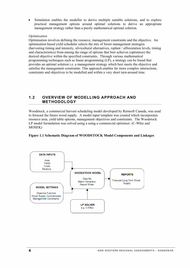
1.2 OVERVIEW OF MODELLING APPROACH ANDMETHODOLOGY
Woodstock, a commercial harvest scheduling model developed by Remsoft Canada, was usedto forecast the future wood supply. A model input template was created which incorporatesresource area, yield table options, management objectives and constraints. The WoodstockLP model formulation was solved using a using a commercial optimiser. (C-Whiz andMOSEK)
Figure 1.1 Schematic Diagram of WOODSTOCK Model Components and Linkages

5 N SW W EST ER N R EG IO N AL A SS ES S MEN T S – N AN D EW AR
Modelling the Nandewar Bioregion wood supply forecasts using Woodstock involves thefollowing steps:
1. Install Woodstock and LP solver software on computer
2. Set up Woodstock model template
(a) Define landscape themes (hierarchical classification of the forest area)
Ten themes were defined for the Nandewar forest resource, which fall into threegeneral categories:
• Geographical areas: Management Area, Forest Name, Timber Price Zone, TimberSupply Zone
• Forest description: silvicultural forest type, stratum• Silvicultural regime applicable in area (silviculture, intensity, return time, delay
period before first harvest event)
(b) Copy formatted net harvest area data generated from Access database onto template.The area classification corresponds to the landscape themes identified in precedingstep.
(c) Copy formatted yield tables generated in Native forest growth and yield simulatoronto template. The yield classification corresponds to the Forest Description(Stratum) and Silvicultural Regime Options (Harvest Delay) landscape themes. Theyield tables are strata level yield tables not yield tables for specific geographicalareas.
(d) Define the modelling Actions applicable to the existing forest resource. The actionsinclude defining each of the Harvest Delay options available for each forest area.Harvest delay Actions are defined for each yield table harvest delay option.
(e) Define the modelling Transitions applicable to the existing forest resource. TheTransitions determine how the declared Actions will be implemented.
(f) Define the planning horizon for model (lifespan) and controls (parameters specifiedto execute your Woodstock forest model).
(g) Define the outputs, graphics and reports from modelling (e.g. volume by location andlog product type).
(h) Define the objective function (e.g. maximise volume of White Cypress pine sawlogover the planning horizon).
(i) Define the constraints (e.g. minimum or maximum volume of a log product volumethat is produced in a given time period, maximum amount of variability permitted inharvest production levels).
3. Solve Woodstock model
n Check model syntax and correct as necessaryn Generated LP matrix, solve LP model and run Woodstock to generate solution reports

6 N SW W EST ER N R EG IO N AL A SS ES S MEN T S – N AN D EW AR
4. Analyse and Report Wood Supply Forecast Resource
n Evaluate the impact of the conservation reserve design on wood production volumeand source of wood. If unsatisfactory (production levels too low or too volatile overtime) or if the modelling result is an infeasible solution, then modify constraints toidentify harvest schedules that provide a higher volume and less irregular woodsupply profiles over time. An infeasible solution will result if wood supply simplycannot meet the constraints from the net harvestable area.
n Report the best results achieved for each Conservation reserve design proposed.

7 N SW W EST ER N R EG IO N AL A SS ES S MEN T S – N AN D EW AR
NATIVE FOREST STRATEGIC YIELD SCHEDULING
2 Area DatabaseThe net harvestable area (NHA) data for the Woodstock file was derived from a customisedNHA Access database developed by SFNSW. Generating a NHA file involves the useridentifying which Forest Management Zones (FMZs) are available for wood production, therange of non-harvestable area exclusions, plus a conservation reserve design that will bededucted from the gross forest area. The NHA database generates a net harvestable area filein the format required for the Woodstock model.
2.1 AREA DEFINITION
The net harvestable area comprises State Forest land holdings available and accessible fortimber production operations. Areas protected by conservation protocols are not included.These are either defined as FMZs that are entirely excluded from timber production practicesor emphasis zones where restricted practices may be applied. The Net Harvest Area is thatcomponent of the land base that is outside the defined timber exclusion areas.
Gross State Forest Area
Less
FMZ 1,2,3a,3f,5,6,7,8
C-PLAN Reserve design (planning units nominated for inclusion in a formal or informalreserve).
User specified exclusions
= Eligible Net Harvestable Area
Less
Net Harvest Area Modifier
= Actual Net Harvestable Area

8 N SW W EST ER N R EG IO N AL A SS ES S MEN T S – N AN D EW AR
Figure 2.1: Net Harvest Area Database User Interface
Land excluded from the definition of the net harvestable area:
n agreed management protocols such as the EPA licence conditions and NPWS generalprotocols;
n NPWS species specific management protocolsn terrain factors (e.g. steep slopes);n accessibility factors (road access);n leasehold conditions (timber availability encumbered by lease conditions);n State Forests forest management priorities (visual quality retention, reserves);n harvesting operation factors (e.g. proximity to buffer zones, rocky or bouldery conditions,
traffic impediments);n economic factors; andn timber merchantability factors.
Exclusions are defined in three ways in the Net Harvest Area Database:
1. Deselection of specific Forest Management Zones2. Selection of specific exclusions3. Net harvest area modifiers
9 N SW W EST ER N R EG IO N AL A SS ES S MEN T S – N AN D EW AR
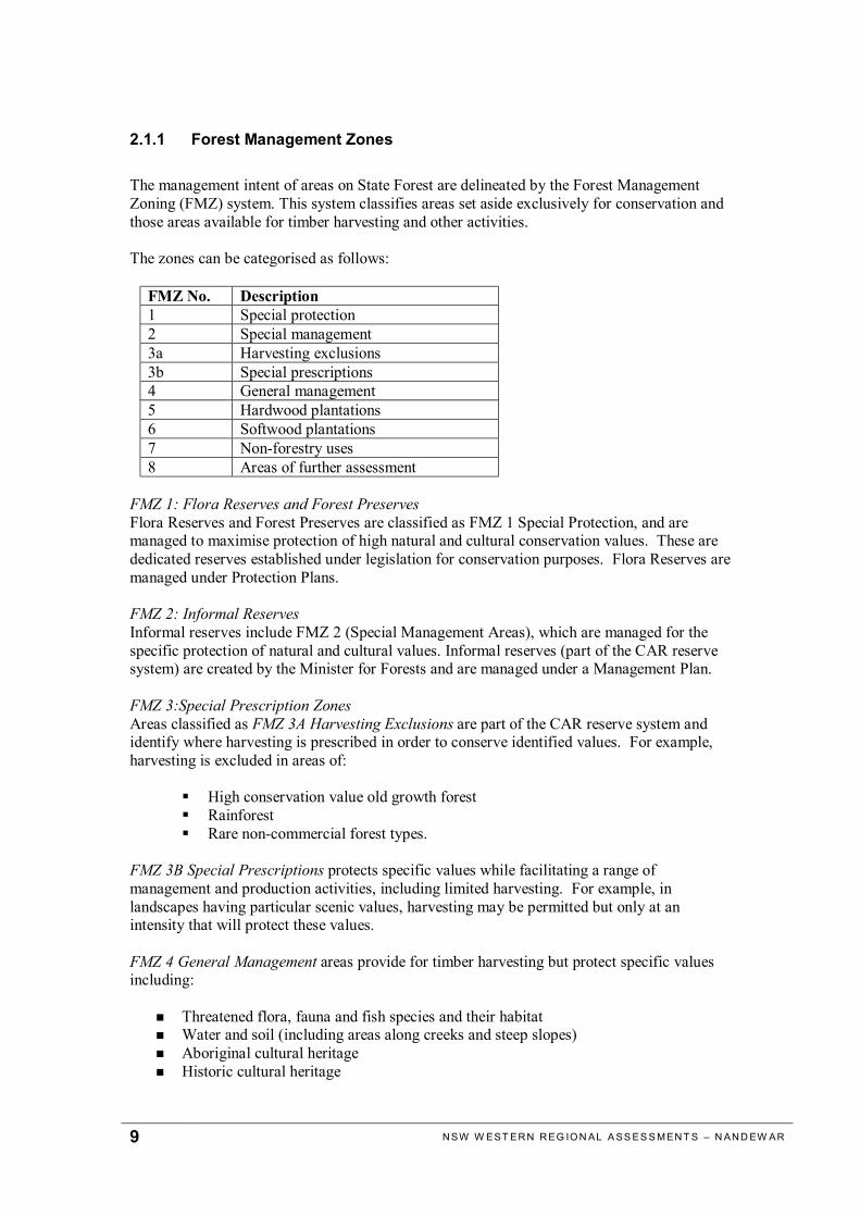
2.1.1 Forest Management Zones
The management intent of areas on State Forest are delineated by the Forest ManagementZoning (FMZ) system. This system classifies areas set aside exclusively for conservation andthose areas available for timber harvesting and other activities.
The zones can be categorised as follows:
FMZ No. Description1 Special protection2 Special management3a Harvesting exclusions3b Special prescriptions4 General management5 Hardwood plantations6 Softwood plantations7 Non-forestry uses8 Areas of further assessment
FMZ 1: Flora Reserves and Forest PreservesFlora Reserves and Forest Preserves are classified as FMZ 1 Special Protection, and aremanaged to maximise protection of high natural and cultural conservation values. These arededicated reserves established under legislation for conservation purposes. Flora Reserves aremanaged under Protection Plans.
FMZ 2: Informal ReservesInformal reserves include FMZ 2 (Special Management Areas), which are managed for thespecific protection of natural and cultural values. Informal reserves (part of the CAR reservesystem) are created by the Minister for Forests and are managed under a Management Plan.
FMZ 3:Special Prescription ZonesAreas classified as FMZ 3A Harvesting Exclusions are part of the CAR reserve system andidentify where harvesting is prescribed in order to conserve identified values. For example,harvesting is excluded in areas of:
§ High conservation value old growth forest§ Rainforest§ Rare non-commercial forest types.
FMZ 3B Special Prescriptions protects specific values while facilitating a range ofmanagement and production activities, including limited harvesting. For example, inlandscapes having particular scenic values, harvesting may be permitted but only at anintensity that will protect these values.
FMZ 4 General Management areas provide for timber harvesting but protect specific valuesincluding:
n Threatened flora, fauna and fish species and their habitatn Water and soil (including areas along creeks and steep slopes)n Aboriginal cultural heritagen Historic cultural heritage
10 N SW W EST ER N R EG IO N AL A SS ES S MEN T S – N AN D EW AR
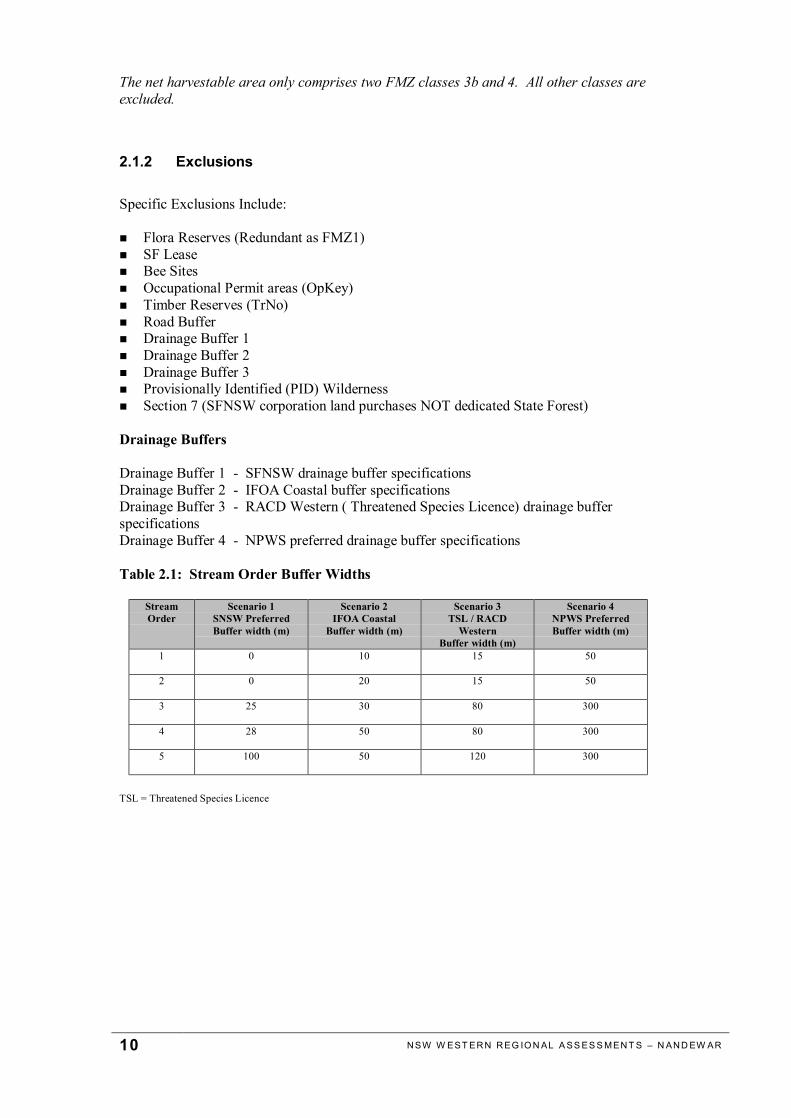
The net harvestable area only comprises two FMZ classes 3b and 4. All other classes areexcluded.
2.1.2 Exclusions
Specific Exclusions Include:
n Flora Reserves (Redundant as FMZ1)n SF Leasen Bee Sitesn Occupational Permit areas (OpKey)n Timber Reserves (TrNo)n Road Buffern Drainage Buffer 1n Drainage Buffer 2n Drainage Buffer 3n Provisionally Identified (PID) Wildernessn Section 7 (SFNSW corporation land purchases NOT dedicated State Forest)
Drainage Buffers
Drainage Buffer 1 - SFNSW drainage buffer specificationsDrainage Buffer 2 - IFOA Coastal buffer specificationsDrainage Buffer 3 - RACD Western ( Threatened Species Licence) drainage bufferspecificationsDrainage Buffer 4 - NPWS preferred drainage buffer specifications
Table 2.1: Stream Order Buffer Widths
StreamOrder
Scenario 1SNSW PreferredBuffer width (m)
Scenario 2IFOA Coastal
Buffer width (m)
Scenario 3TSL / RACD
WesternBuffer width (m)
Scenario 4NPWS PreferredBuffer width (m)
1 0 10 15 50
2 0 20 15 50
3 25 30 80 300
4 28 50 80 300
5 100 50 120 300
TSL = Threatened Species Licence

11 N SW W EST ER N R EG IO N AL A SS ES S MEN T S – N AN D EW AR
2.1.3 Net Harvest Area Modifier
A net harvest area modifier is an area reduction factor, used to account for the probability thatpart of the available (mapped) harvestable area will not be harvested due to unmapped and/orunmappable factors additional to the general Ecologically Sustainable Forest Management(ESFM) protocols.
The difference between the eligible harvest area and actual harvest area was based on asample selection of compartments within State Forests in the Nandewar Bioregion whereharvesting has occurred between 1997 and 2003 and aerial photo coverage (2001/02) wasavailable. Changes to logging protocols since harvesting were addressed in the analysis. Thecurrent harvest plan boundaries were superimposed on the aerial photos.
Detailed survey records were used to derive a statistical formula to determine the likelihoodthat a given net harvestable area would not be harvested during a thinning or releaseharvesting operation. The statistical formula was applied to the entire area of State Forest inthe Nandewar Bioregion using a GIS Grid. A ratio of actual harvested area to the eligiblearea was generated separately for a 25m grid cell that makes each spatial analysis unit. Theweighted average ratios are provided for each analysis unit in the NHA database.
The NHAM excludes non-commercial and pre-commercial components of the eligible area,which was not harvested in the compartment sample. These are captured in the simulation ofthe strategic inventory plots. Non-commercial species are not harvested and are part of thegrowing stock of the modelled forest and do not contribute any yield. A tree with quotaquality wood but, does not yet meet diameter specifications is available to harvest in thefuture.
Similarly, areas excluded from harvesting because there are too few merchantable trees perhectare for a viable harvesting operation are also captured through the inventory. The growthof these areas is simulated over time and if an adequate economic volume of high qualitysawlog grows they areas will be harvested, if not, they simply remain part of the growingstock and do not contribute to the yield.
In the strategic inventory individual trees were assigned tree availability status. Unavailabletree categories included: habitat trees, environmental buffers, unmapped physicalimpediments and undefined other factors. The environmental buffers are addressed throughthe NHA exclusions and unmapped physical impediments (e.g. cliffs, steep areas notidentified on the GIS, presence of rock) are addressed through the NHAM.

12 N SW W EST ER N R EG IO N AL A SS ES S MEN T S – N AN D EW AR
2.2 LAND ATTRIBUTES
Table 2.2: Net Harvest Area By Geographical Location & Stratum
Stratum Timber PriceZone (TPZ)
TPZ no. TimberSupply Zone
(TSZ)
TSZ no. SilviculturalForest Type
Group
NHA (ha)
1 Gunnedah 5 Gunnedah 4 MIX 286.61 Gunnedah 5 Gunnedah 4 WCP 103.31 Gunnedah 5 Attunga 10 MIX 53.11 Gunnedah 5 Attunga 10 WCP 98.11 Inverell 6 Inverell 5 IBK 1,305.91 Inverell 6 Inverell 5 MIX 12,463.11 Inverell 6 Inverell 5 WCP 301.4
Sub Total 14,6112 Gunnedah 5 Gunnedah 4 MIX 34.12 Gunnedah 5 Gunnedah 4 WCP 9.92 Gunnedah 5 Attunga 10 MIX 21.42 Gunnedah 5 Attunga 10 WCP 28.32 Inverell 6 Inverell 5 IBK 26.92 Inverell 6 Inverell 5 MIX 3,709.72 Inverell 6 Inverell 5 WCP 81.7
Sub Total 3,912Total Area 18,523
NHA based on exclusion of Threatened Species Licence Stream Buffer widths.
2.2.1 Timber Supply Zone
Timber Supply Zones (TSZ) are small groups of compartments within a Timber Catchmentthat have similar timber resource characteristics and silvicultural requirements. These arelogical self-contained timber management units in terms of infrastructure and geographicalboundaries. The Timber Supply Zones provide a good geographical basis for reporting theoptions’ source of wood when evaluating wood supply options.
TSZ 4 = GunnedahTSZ 5 = InverellTSZ 10 = Attunga

13 N SW W EST ER N R EG IO N AL A SS ES S MEN T S – N AN D EW AR
2.2.2 Timber Price Zone
Timber Price Zones (TPZ) are geographically contiguous areas with similar log royaltystructures based on timber species groups, harvesting terrain and haulage distance to markets.The Timber Price Zones provide a useful geographical basis for reporting the source of woodwhen evaluating wood supply options.
The Nandewar TPZ includes:TPZ5 = GunnedahTPZ6 = Inverell
2.2.3 Silvicultural Forest Types
The area database was structured with broad silvicultural forest type definitions. These aregroups of forest types originally aimed at separating the resource by silvicultural intent.
The silvicultural forest type groups are:
• WCP (cypress dominated stands with little or no commercial ironbark)i.e Cypress Pine-Box
• IBK (ironbark dominated stands with little or no commercial cypress)i.e. Ironbark Dominant, No commercial Cypress
• MIX (cypress and ironbark mixed stand both in commercial quantities) Cypress Pine-Ironbark, Cypress Pine-Redgum
The silvicultural forest types provide a good geographical basis for reporting the source ofwood when evaluating wood supply options.
Only WCP was used for Nandewar Bioregion.
14 N SW W EST ER N R EG IO N AL A SS ES S MEN T S – N AN D EW AR
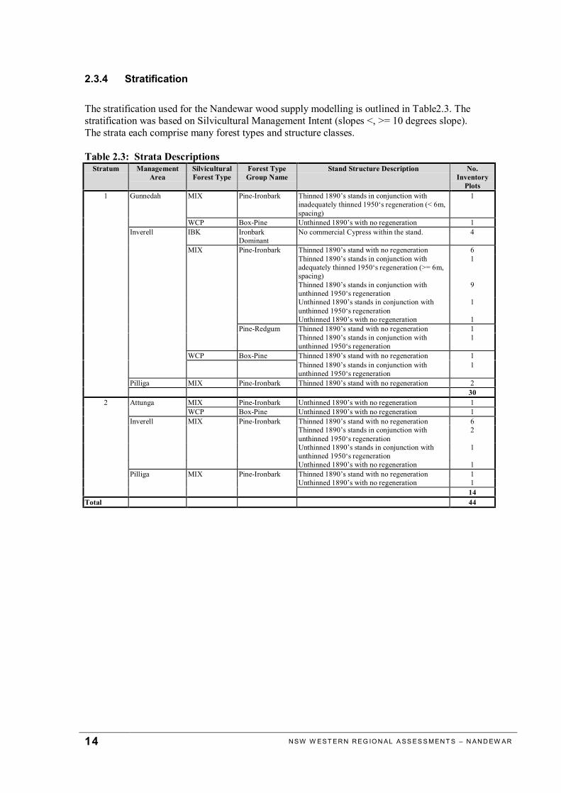
2.3.4 Stratification
The stratification used for the Nandewar wood supply modelling is outlined in Table2.3. Thestratification was based on Silvicultural Management Intent (slopes <, >= 10 degrees slope).The strata each comprise many forest types and structure classes.
Table 2.3: Strata DescriptionsStratum Management
AreaSilviculturalForest Type
Forest TypeGroup Name
Stand Structure Description No.Inventory
PlotsMIX Pine-Ironbark Thinned 1890’s stands in conjunction with
inadequately thinned 1950‘s regeneration (< 6m,spacing)
1Gunnedah
WCP Box-Pine Unthinned 1890’s with no regeneration 1IBK Ironbark
DominantNo commercial Cypress within the stand. 4
Thinned 1890’s stand with no regeneration 6Thinned 1890’s stands in conjunction withadequately thinned 1950‘s regeneration (>= 6m,spacing)
1
Thinned 1890’s stands in conjunction withunthinned 1950‘s regeneration
9
Unthinned 1890’s stands in conjunction withunthinned 1950‘s regeneration
1
Pine-Ironbark
Unthinned 1890’s with no regeneration 1Thinned 1890’s stand with no regeneration 1
MIX
Pine-RedgumThinned 1890’s stands in conjunction withunthinned 1950‘s regeneration
1
WCP Box-Pine Thinned 1890’s stand with no regeneration 1
Inverell
Thinned 1890’s stands in conjunction withunthinned 1950‘s regeneration
1
Pilliga MIX Pine-Ironbark Thinned 1890’s stand with no regeneration 2
1
30MIX Pine-Ironbark Unthinned 1890’s with no regeneration 1AttungaWCP Box-Pine Unthinned 1890’s with no regeneration 1
Thinned 1890’s stand with no regeneration 6Thinned 1890’s stands in conjunction withunthinned 1950‘s regeneration
2
Unthinned 1890’s stands in conjunction withunthinned 1950‘s regeneration
1
Inverell MIX Pine-Ironbark
Unthinned 1890’s with no regeneration 1Thinned 1890’s stand with no regeneration 1Pilliga MIX Pine-IronbarkUnthinned 1890’s with no regeneration 1
2
14Total 44

15 N SW W EST ER N R EG IO N AL A SS ES S MEN T S – N AN D EW AR
Where:
Silvicultural Forest TypesIBK = Ironbark sppWCP = White Cypress PineMIX = Mixed species
Forest Type GroupThere are 4 broad forest types in the Nandewar Bioregion that aredominated by two commercial species - White Cypress Pine and Ironbark species.• Cypress Pine-Box• Cypress Pine-Ironbark• Cypress Pine-Redgum• Ironbark Dominant
The forest groups are amalgamations of Lindsay forest types (Lindsay, 1967) as outlined inTable 2.4.
Stand StructureThe following 10 stand structure classes (Forest Management History) were used to defineWestern region forest structure. These are focussed on the White Cypress Pine component ofthe stand.
1. Thinned 1890’s stand with no regeneration2. Thinned 1890’s stands in conjunction with inadequately thinned 1950‘s regeneration
(< 6m, spacing)3. Thinned 1890’s stands in conjunction with adequately thinned 1950‘s regeneration
(>= 6m, spacing)4. Thinned 1890’s stands in conjunction with unthinned 1950‘s regeneration5. Unthinned 1890’s with no regeneration6. Unthinned 1890’s stands in conjunction with unthinned 1950‘s regeneration7. Inadequately thinned 1950‘s (< 6m, spacing) regeneration8. Adequately thinned 1950‘s (>= 6m, spacing) regeneration9. Unthinned 1950’s regeneration10. No commercial Cypress within the stand.

16 N SW W EST ER N R EG IO N AL A SS ES S MEN T S – N AN D EW AR
Table 2.4: Lindsay type groupings used in Nandewar Bioregion
LINDSAY GROUP NAME DESCRIPTION OF COMPOSTION
White Cypress Pine / Box types Dominated by Lindsay types:PgP Pilliga Box-PinePPf Pine-Bimble BoxPPg Pine-Pilliga BoxWith minor associations of types:PCn Pine-Fuzzy BoxPf Bimble BoxPfP Bimble Box-PinePg Pilliga BoxPgBP Pilliga Box-Red Gum-PinePgPf Pilliga Box-Bimble BoxPH Pine-White BoxPPgC Pine-Pilliga Box-Narrow leaved Ironbark
Ironbark Eucalypt Dominant Dominated by types:NT Broad leaved Ironbark-BloodwoodNTBp Broad leaved Ironbark-Bloodwood-Black PineCT Narrow leaved Ironbark-BloodwoodC Narrow leaved IronbarkN Broad leaved IronbarkNTBr Broad leaved Ironbark-Bloodwood-BroomTNBp Bloodwood-Broad leaved Ironbark-Black Pine
White Cypress Pine /Ironbark The most dominant group in the Pilliga.Dominated by types:COP Narrow leaved Ironbark-Forest Oak-PinePCO Pine-Narrow leaved Ironbark-Forest OakDominating other minor types:BCP Red Gum-Narrow leaved Ironbark-PinePCB Pine-Narrow leaved Ironbark-Red GumTBCP Bloodwood-Red Gum-Narrow leaved Ironbark-Pine
White Cypress Pine/ Red Gum Types This is primarily dominated by the red gum types:BAP Red Gum-Roughbarked Apple-PineBNBp Red Gum-Broad leaved Ironbark-Black PineBNP Red Gum-Broad leaved Ironbark-PineBP Red Gum-PinePB Pine-Red GumPBA Pine-Red Gum-Roughbarked Apple
17 N SW W EST ER N R EG IO N AL A SS ES S MEN T S – N AN D EW AR
2.3 WOODSTOCK AREA FILE STRUCTURE AND FORMAT
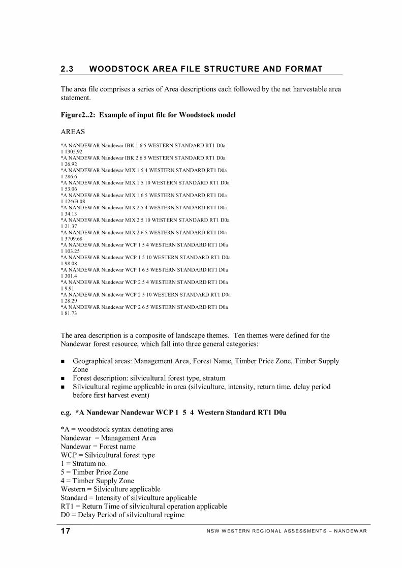
The area file comprises a series of Area descriptions each followed by the net harvestable areastatement.
Figure2..2: Example of input file for Woodstock model
AREAS
*A NANDEWAR Nandewar IBK 1 6 5 WESTERN STANDARD RT1 D0a1 1305.92*A NANDEWAR Nandewar IBK 2 6 5 WESTERN STANDARD RT1 D0a1 26.92*A NANDEWAR Nandewar MIX 1 5 4 WESTERN STANDARD RT1 D0a1 286.6*A NANDEWAR Nandewar MIX 1 5 10 WESTERN STANDARD RT1 D0a1 53.06*A NANDEWAR Nandewar MIX 1 6 5 WESTERN STANDARD RT1 D0a1 12463.08*A NANDEWAR Nandewar MIX 2 5 4 WESTERN STANDARD RT1 D0a1 34.13*A NANDEWAR Nandewar MIX 2 5 10 WESTERN STANDARD RT1 D0a1 21.37*A NANDEWAR Nandewar MIX 2 6 5 WESTERN STANDARD RT1 D0a1 3709.68*A NANDEWAR Nandewar WCP 1 5 4 WESTERN STANDARD RT1 D0a1 103.25*A NANDEWAR Nandewar WCP 1 5 10 WESTERN STANDARD RT1 D0a1 98.08*A NANDEWAR Nandewar WCP 1 6 5 WESTERN STANDARD RT1 D0a1 301.4*A NANDEWAR Nandewar WCP 2 5 4 WESTERN STANDARD RT1 D0a1 9.91*A NANDEWAR Nandewar WCP 2 5 10 WESTERN STANDARD RT1 D0a1 28.29*A NANDEWAR Nandewar WCP 2 6 5 WESTERN STANDARD RT1 D0a1 81.73
The area description is a composite of landscape themes. Ten themes were defined for theNandewar forest resource, which fall into three general categories:
n Geographical areas: Management Area, Forest Name, Timber Price Zone, Timber SupplyZone
n Forest description: silvicultural forest type, stratumn Silvicultural regime applicable in area (silviculture, intensity, return time, delay period
before first harvest event)
e.g. *A Nandewar Nandewar WCP 1 5 4 Western Standard RT1 D0a
*A = woodstock syntax denoting areaNandewar = Management AreaNandewar = Forest nameWCP = Silvicultural forest type1 = Stratum no.5 = Timber Price Zone4 = Timber Supply ZoneWestern = Silviculture applicableStandard = Intensity of silviculture applicableRT1 = Return Time of silvicultural operation applicableD0 = Delay Period of silvicultural regime

18 N SW W EST ER N R EG IO N AL A SS ES S MEN T S – N AN D EW AR
Landscape
The options for each theme defined in the Nandewar Bioregion are:
1. Management AreaNandewar (includes Attunga, Gunnedah, Inverell, Pilliga)
2. ForestNandewar
3. Silvicultural Forest TypeIBK, MIX, WBK, WCP
4. Stratum1 and 2
5. TPZ5 and 6
6. TSZ4, 5 & 10
7. SilvicultureWestern
8. IntensityStandard
9. Return TimeRT1
10. Delay(a) delays assigned to existing forest classesD0a Nil, D1a years, D2a, D3a, D4a, D5a, D6a, D7a, D8a, D9a, D10a
(b) delays assigned by WoodstockD0 Nil, D1 5years, D2, D3, D4, D5, D6, D7, D8, D9, D10
19 N SW W EST ER N R EG IO N AL A SS ES S MEN T S – N AN D EW AR
NATIVE FOREST STRATEGIC YIELD SCHEDULING
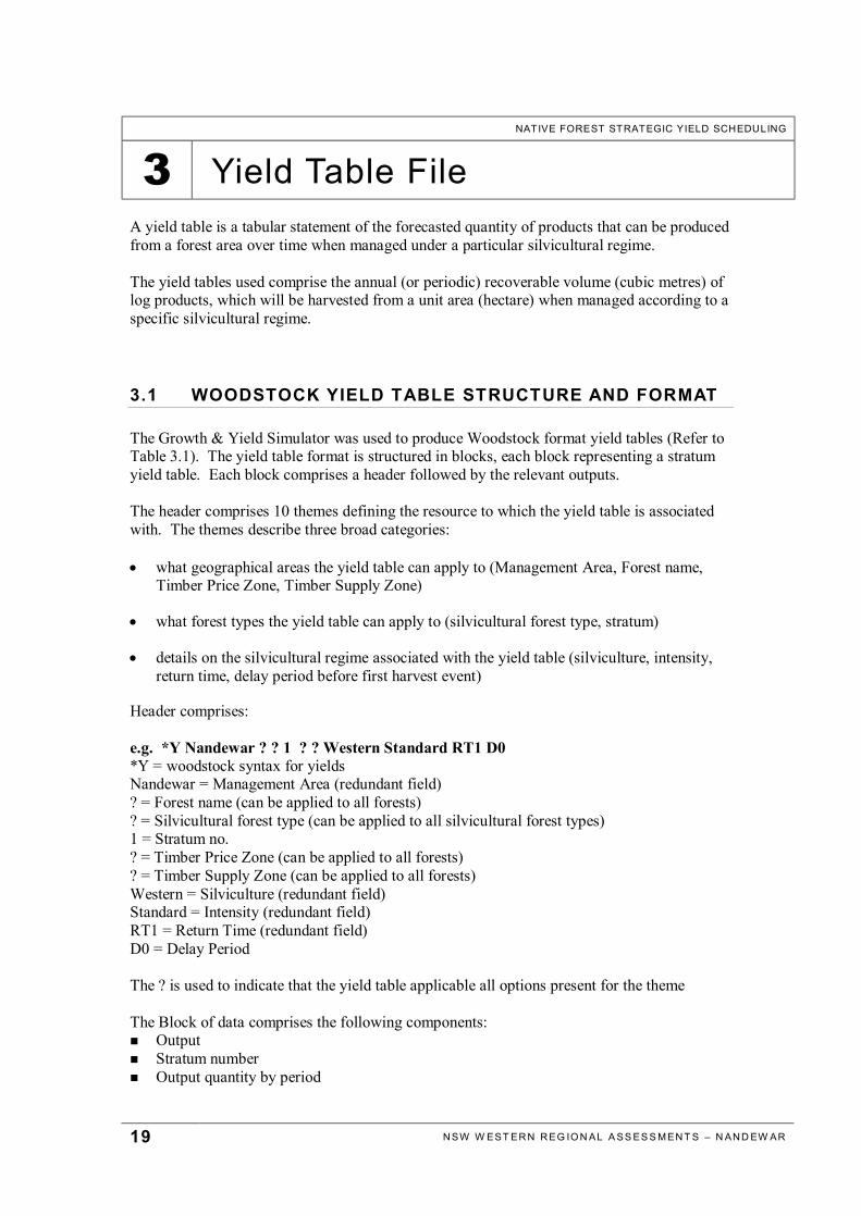
3 Yield Table FileA yield table is a tabular statement of the forecasted quantity of products that can be producedfrom a forest area over time when managed under a particular silvicultural regime.
The yield tables used comprise the annual (or periodic) recoverable volume (cubic metres) oflog products, which will be harvested from a unit area (hectare) when managed according to aspecific silvicultural regime.
3.1 WOODSTOCK YIELD TABLE STRUCTURE AND FORMAT
The Growth & Yield Simulator was used to produce Woodstock format yield tables (Refer toTable 3.1). The yield table format is structured in blocks, each block representing a stratumyield table. Each block comprises a header followed by the relevant outputs.
The header comprises 10 themes defining the resource to which the yield table is associatedwith. The themes describe three broad categories:
• what geographical areas the yield table can apply to (Management Area, Forest name,Timber Price Zone, Timber Supply Zone)
• what forest types the yield table can apply to (silvicultural forest type, stratum)
• details on the silvicultural regime associated with the yield table (silviculture, intensity,return time, delay period before first harvest event)
Header comprises:
e.g. *Y Nandewar ? ? 1 ? ? Western Standard RT1 D0*Y = woodstock syntax for yieldsNandewar = Management Area (redundant field)? = Forest name (can be applied to all forests)? = Silvicultural forest type (can be applied to all silvicultural forest types)1 = Stratum no.? = Timber Price Zone (can be applied to all forests)? = Timber Supply Zone (can be applied to all forests)Western = Silviculture (redundant field)Standard = Intensity (redundant field)RT1 = Return Time (redundant field)D0 = Delay Period
The ? is used to indicate that the yield table applicable all options present for the theme
The Block of data comprises the following components:n Outputn Stratum numbern Output quantity by period

20 N SW W EST ER N R EG IO N AL A SS ES S MEN T S – N AN D EW AR
Outputs include:HQ_Large_Yield_IBK = Yield of high quality Ironbark sawlogsHQ_Large_Yield_WCP = Yield of high quality White Cypress Pine sawlogsNCT_Prop_Area = Proportion of Area which received a Non-Commercial Thinning operationCT_Prop_Area = Proportion of Area which received a Commercial Thinning operationR_Prop_Area = Proportion of Area which received a Release harvest operationHQ_IBK_GS_Vol = Standing crop volume of high quality Ironbark sawlogsHQ_WCP_GS_Vol = Standing crop volume of high quality White Cypress Pine sawlogsHQ_OTH_GS_Vol = Standing crop volume of high quality Other Species sawlogsWaste_IBK_GS_Vol = Standing crop volume of waste quality Ironbark sawlogsWaste_WCP_GS_Vol = Standing crop volume of waste quality White Cypress Pine sawlogsWaste_OTH_GS_Vol = Standing crop volume of waste quality Other Species sawlogsIBK_GS_BA = Standing crop basal area of waste quality Ironbark sawlogsWCP_GS_BA = Standing crop basal area of waste quality White Cypress Pine sawlogsOTH_GS_BA = Standing crop basal area of waste quality Other Species sawlogsIBK_GS_STKG = Standing crop stocking of waste quality Ironbark sawlogsWCP_GS_STKG = Standing crop stocking of waste quality White Cypress Pine sawlogsOTH_GS_STKG = Standing crop stocking of waste quality Other Species sawlogs
• The yields are expressed as average annual volume (m3/ha) for the defined period.• The areas are expressed as average proportion of area treated annually for the defined
period.• The standing crop volume expressed as average volume (m3/ha)for the defined period (not
start, mid or end point)• The standing crop basal area expressed as average basal area(m2/ha)for the defined period
(not start, mid or end point)• The standing crop stocking expressed as average stocking (stems/ha)for the defined
period (not start, mid or end point)
• The output quantities are provided for each period of the planning horizon (these aresuccessive numbers along the same line of data). Each figure is the annual averagequantity

21 N SW W EST ER N R EG IO N AL A SS ES S MEN T S – N AN D EW AR
Table 3.1: Excerpt from Woodstock File Yield Table
*Y Nandewar ? WCP 1 ? ? Western Standard RT1 D0HQ_Large_Yield_IBK 1 0.000 0.000 0.000 0.000 0.000 0.000 0.000 0.000 0.000 0.000 0.000 0.000 0.000 0.000 0.000 0.000 0.000 0.000 0.000 0.000 0.000 0.000 0.000 0.000 0.000 0.000 0.000 0.000 0.000 0.000 0.000 0.000 0.000 0.000 0.000 0.000 0.000 0.000 0.000 0.000HQ_Large_Yield_WCP 1 1.525 0.000 0.028 0.000 0.087 0.028 1.202 0.155 0.456 0.057 0.429 0.167 0.232 0.091 0.297 0.175 0.472 0.052 0.238 0.141 0.359 0.045 0.054 0.089 0.403 0.223 0.119 0.074 0.222 0.072 0.068 0.064 0.375 0.081 0.227 0.089 0.268 0.034 0.200 0.164NCT_Prop_Area 1 0.000 0.000 0.007 0.000 0.000 0.000 0.000 0.000 0.040 0.000 0.000 0.000 0.013 0.000 0.000 0.000 0.013 0.000 0.007 0.000 0.000 0.000 0.013 0.000 0.000 0.000 0.027 0.000 0.007 0.000 0.000 0.000 0.000 0.000 0.000 0.000 0.013 0.000 0.007 0.000CT_Prop_Area 1 0.067 0.000 0.007 0.000 0.013 0.007 0.020 0.020 0.047 0.013 0.013 0.020 0.020 0.013 0.033 0.020 0.027 0.007 0.053 0.020 0.033 0.007 0.013 0.020 0.033 0.020 0.013 0.013 0.040 0.013 0.013 0.013 0.060 0.020 0.013 0.020 0.040 0.007 0.020 0.027R_Prop_Area 1 0.007 0.000 0.000 0.000 0.000 0.000 0.040 0.000 0.000 0.000 0.013 0.000 0.000 0.000 0.013 0.000 0.007 0.000 0.000 0.000 0.013 0.000 0.000 0.000 0.027 0.000 0.007 0.000 0.000 0.000 0.000 0.000 0.000 0.000 0.013 0.000 0.007 0.000 0.013 0.007HQ_IBK_GS_Vol 1 0.115 0.163 0.192 0.199 0.188 0.188 0.209 0.243 0.275 0.293 0.324 0.381 0.446 0.493 0.529 0.566 0.557 0.547 0.532 0.519 0.516 0.513 0.505 0.496 0.488 0.491 0.495 0.498 0.498 0.504 0.517 0.519 0.513 0.521 0.536 0.527 0.522 0.515 0.501 0.509HQ_WCP_GS_Vol 1 7.727 7.260 8.125 9.387 10.569 12.106 8.808 8.598 7.441 7.513 7.149 7.047 7.004 7.232 6.984 7.289 6.174 5.989 6.306 6.374 5.871 5.993 6.550 7.105 7.292 6.825 6.294 6.353 6.553 6.423 7.002 7.405 7.491 6.835 7.210 7.157 7.211 7.007 7.553 7.270Waste_IBK_GS_Vol 1 6.801 7.829 8.036 8.243 8.494 8.634 8.697 8.860 9.023 9.077 9.207 9.262 9.384 9.547 9.638 9.841 10.010 10.160 10.200 10.362 10.559 10.674 10.799 10.834 10.803 10.863 10.915 10.927 10.956 10.996 11.079 10.954 10.915 10.885 10.757 10.579 10.462 10.410 10Waste_WCP_GS_Vol 1 13.578 14.445 15.134 16.109 17.112 18.372 17.977 18.732 17.990 18.326 19.287 20.403 21.417 22.267 23.193 24.498 24.373 24.455 25.431 26.167 26.779 27.365 27.606 27.927 28.307 28.566 28.682 28.433 28.836 29.130 29.798 30.332 30.797 31.046 31.728 32.065 Waste_OTH_GS_Vol 1 112.798 115.707 115.883 115.862 115.139 114.834 113.838 113.434 109.519 108.926 109.573 108.922 108.087 108.105 107.884 108.146 107.588 106.588 105.554 105.007 103.924 102.870 101.757 100.710 100.021 99.590 98.791 98.939 97.982 97.529 97.473 96.601 95.IBK_GS_BA 1 1.5 1.5 1.6 1.6 1.6 1.7 1.7 1.7 1.7 1.8 1.8 1.8 1.8 1.9 1.9 1.9 1.9 2.0 2.0 2.0 2.0 2.0 2.0 2.0 2.0 2.0 2.0 2.0 2.0 2.0 2.0 2.0 2.0 2.0 2.0 1.9 1.9 1.9 1.9 1.9WCP_GS_BA 1 3.9 4.0 4.3 4.7 5.0 5.4 4.8 4.9 4.8 4.7 4.8 4.9 5.1 5.2 5.3 5.5 5.2 5.1 5.3 5.4 5.4 5.5 5.7 5.7 5.8 5.7 5.8 5.7 5.8 5.8 6.0 6.1 6.2 6.1 6.2 6.3 6.3 6.3 6.5 6.4OTH_GS_BA 1 9.0 9.1 9.1 9.2 9.4 9.4 9.5 9.5 9.5 9.5 9.6 9.6 9.6 9.6 9.6 9.6 9.6 9.5 9.5 9.5 9.4 9.4 9.3 9.3 9.2 9.2 9.2 9.2 9.0 9.0 8.9 8.9 8.8 8.8 8.7 8.6 8.6 8.5 8.5 8.5IBK_GS_STKG 1 41 41 41 41 42 41 41 41 41 41 41 40 41 41 40 40 40 39 39 38 38 37 37 36 35 35 35 34 34 34 34 33 33 33 33 32 32 32 31 31WCP_GS_STKG 1 167 207 227 224 225 230 209 205 270 217 213 212 233 217 212 209 202 172 189 178 173 170 193 175 173 167 203 179 190 181 182 181 179 172 171 168 187 172 182 175OTH_GS_STKG 1 230 229 226 225 223 221 217 214 207 204 202 199 197 196 194 194 193 190 187 184 181 178 176 173 171 169 167 166 164 162 160 158 156 154 152 150 149 147 147 146
*Y Nandewar ? WCP 1 ? ? Western Standard RT1 D1HQ_Large_Yield_IBK 1 0.000 0.000 0.000 0.000 0.000 0.000 0.000 0.000 0.000 0.000 0.000 0.000 0.000 0.000 0.000 0.000 0.000 0.000 0.000 0.000 0.000 0.000 0.000 0.000 0.000 0.000 0.000 0.000 0.000 0.000 0.000 0.000 0.000 0.000 0.000 0.000 0.000 0.000 0.000 0.000HQ_Large_Yield_WCP 1 0.000 1.490 0.028 0.000 0.000 0.064 0.218 1.194 0.237 0.243 0.465 0.232 0.141 0.107 0.173 0.381 0.417 0.076 0.112 0.223 0.134 0.171 0.136 0.231 0.119 0.137 0.188 0.095 0.251 0.211 0.100 0.114 0.109 0.165 0.099 0.243 0.255 0.093 0.058 0.166NCT_Prop_Area 1 0.000 0.000 0.000 0.007 0.000 0.000 0.000 0.000 0.000 0.040 0.000 0.000 0.007 0.000 0.000 0.000 0.007 0.007 0.013 0.000 0.000 0.000 0.000 0.020 0.000 0.000 0.000 0.007 0.000 0.000 0.013 0.000 0.000 0.007 0.000 0.000 0.000 0.020 0.000 0.000CT_Prop_Area 1 0.000 0.067 0.007 0.000 0.000 0.013 0.020 0.020 0.020 0.027 0.027 0.033 0.013 0.020 0.027 0.040 0.027 0.013 0.027 0.033 0.020 0.007 0.027 0.047 0.020 0.020 0.013 0.020 0.020 0.040 0.020 0.013 0.027 0.033 0.020 0.007 0.047 0.020 0.013 0.013R_Prop_Area 1 0.000 0.007 0.000 0.000 0.000 0.000 0.000 0.040 0.000 0.000 0.007 0.000 0.000 0.000 0.007 0.007 0.013 0.000 0.000 0.000 0.000 0.020 0.000 0.000 0.000 0.007 0.000 0.000 0.013 0.000 0.000 0.007 0.000 0.000 0.000 0.020 0.000 0.000 0.000 0.013HQ_IBK_GS_Vol 1 0.109 0.154 0.183 0.184 0.181 0.179 0.199 0.245 0.281 0.313 0.368 0.428 0.497 0.537 0.572 0.596 0.600 0.596 0.587 0.558 0.543 0.522 0.516 0.508 0.502 0.489 0.483 0.477 0.469 0.465 0.454 0.448 0.450 0.444 0.442 0.443 0.431 0.418 0.390 0.396HQ_WCP_GS_Vol 1 13.201 8.139 7.709 8.875 10.372 11.771 12.768 9.460 8.622 7.831 8.183 6.992 6.861 7.055 7.562 6.832 5.895 5.372 5.975 6.053 6.111 6.189 6.639 6.294 6.178 6.427 6.805 6.606 6.612 6.437 6.491 6.601 6.845 7.106 7.234 7.390 6.807 6.614 6.886 7.133Waste_IBK_GS_Vol 1 6.528 7.779 7.889 8.036 8.283 8.571 8.784 8.790 8.829 8.996 9.096 9.214 9.247 9.377 9.562 9.601 9.691 9.896 10.065 10.212 10.439 10.547 10.694 10.848 11.045 11.160 11.288 11.307 11.349 11.387 11.413 11.359 11.186 11.107 11.071 11.089 11.092 11.135 11.0Waste_WCP_GS_Vol 1 15.209 14.378 15.151 15.762 16.707 17.889 18.897 18.557 19.243 18.959 19.806 20.513 21.748 23.094 24.349 25.276 25.800 25.922 27.092 27.654 28.482 29.243 29.940 29.922 29.922 30.477 31.111 31.470 31.617 31.838 32.332 32.836 33.222 33.640 33.968 34.386 34.517 34.578 34.866 35.218Waste_OTH_GS_Vol 1 111.336 114.642 115.755 117.051 118.076 117.747 117.220 116.655 115.760 112.466 111.448 111.060 110.907 109.644 109.419 109.445 108.397 107.499 106.602 106.044 105.713 105.207 104.763 103.573 102.761 101.840 101.333 100.359 99.747 99.045 97.490 96.712 IBK_GS_BA 1 1.5 1.5 1.5 1.6 1.6 1.7 1.7 1.7 1.7 1.8 1.8 1.8 1.8 1.8 1.9 1.9 1.9 1.9 2.0 2.0 2.0 2.0 2.0 2.0 2.1 2.1 2.1 2.1 2.1 2.1 2.1 2.1 2.1 2.1 2.0 2.0 2.0 2.0 2.0 2.0WCP_GS_BA 1 5.0 4.2 4.3 4.6 4.9 5.3 5.6 5.0 5.0 5.0 5.0 4.9 5.1 5.3 5.6 5.6 5.4 5.2 5.6 5.6 5.7 5.8 6.0 6.0 5.9 6.0 6.1 6.2 6.2 6.1 6.3 6.3 6.4 6.6 6.6 6.7 6.6 6.6 6.6 6.7OTH_GS_BA 1 8.4 8.4 8.6 8.7 8.8 8.9 8.9 9.0 9.0 9.0 9.0 9.0 9.1 9.1 9.1 9.1 9.1 9.1 9.0 9.0 9.0 9.0 8.9 8.8 8.7 8.7 8.6 8.6 8.5 8.5 8.4 8.3 8.3 8.2 8.2 8.1 8.0 8.0 7.9 7.8IBK_GS_STKG 1 41 41 41 41 42 42 42 42 41 41 41 41 40 40 40 39 39 39 39 38 38 38 38 38 37 37 37 36 36 37 37 36 36 36 35 35 35 35 35 35WCP_GS_STKG 1 199 215 222 232 228 230 231 209 201 273 222 215 225 221 220 212 198 185 202 186 184 180 178 204 180 178 178 186 177 172 196 184 183 192 183 180 173 199 183 180OTH_GS_STKG 1 230 231 231 227 225 223 219 216 212 205 202 199 197 194 192 190 187 184 182 180 178 176 174 172 171 169 167 165 163 162 159 156 153 151 151 149 147 145 143 142
*Y Nandewar ? WCP 1 ? ? Western Standard RT1 D2HQ_Large_Yield_IBK 1 0.000 0.000 0.000 0.000 0.000 0.000 0.000 0.000 0.000 0.000 0.000 0.000 0.000 0.000 0.000 0.000 0.000 0.000 0.000 0.000 0.000 0.000 0.000 0.000 0.000 0.000 0.000 0.000 0.000 0.000 0.000 0.000 0.000 0.000 0.000 0.000 0.000 0.000 0.000 0.000HQ_Large_Yield_WCP 1 0.000 0.000 1.695 0.000 0.000 0.000 0.524 0.152 0.791 0.027 0.290 0.241 0.455 0.042 0.578 0.235 0.255 0.058 0.135 0.132 0.196 0.108 0.178 0.196 0.104 0.036 0.325 0.275 0.180 0.110 0.221 0.210 0.141 0.040 0.188 0.112 0.115 0.166 0.150 0.213NCT_Prop_Area 1 0.000 0.000 0.000 0.000 0.007 0.000 0.000 0.000 0.000 0.000 0.020 0.000 0.007 0.000 0.013 0.007 0.013 0.000 0.007 0.000 0.000 0.000 0.000 0.000 0.007 0.007 0.000 0.000 0.013 0.007 0.000 0.000 0.000 0.007 0.000 0.000 0.007 0.007 0.000 0.007CT_Prop_Area 1 0.000 0.000 0.073 0.000 0.000 0.000 0.053 0.020 0.020 0.007 0.033 0.033 0.013 0.000 0.027 0.033 0.020 0.013 0.020 0.020 0.027 0.027 0.027 0.027 0.013 0.007 0.020 0.033 0.033 0.020 0.020 0.027 0.033 0.007 0.027 0.013 0.027 0.027 0.033 0.020R_Prop_Area 1 0.000 0.000 0.007 0.000 0.000 0.000 0.000 0.000 0.020 0.000 0.007 0.000 0.013 0.007 0.013 0.000 0.007 0.000 0.000 0.000 0.000 0.000 0.007 0.007 0.000 0.000 0.013 0.007 0.000 0.000 0.000 0.007 0.000 0.000 0.007 0.007 0.000 0.007 0.000 0.007HQ_IBK_GS_Vol 1 0.114 0.171 0.195 0.204 0.201 0.201 0.214 0.236 0.272 0.298 0.350 0.397 0.446 0.493 0.530 0.555 0.573 0.582 0.569 0.551 0.548 0.542 0.522 0.516 0.515 0.509 0.502 0.502 0.495 0.482 0.473 0.481 0.484 0.477 0.478 0.486 0.488 0.492 0.504 0.498HQ_WCP_GS_Vol 1 13.218 14.154 8.583 8.223 9.484 10.906 10.541 11.171 9.019 9.362 9.299 9.797 8.134 8.314 7.320 6.754 5.642 5.592 5.842 6.413 6.110 6.438 6.535 6.816 6.554 7.082 7.124 6.835 6.077 6.253 6.077 5.683 5.785 6.006 6.306 6.564 6.767 6.808 6.710 6.591Waste_IBK_GS_Vol 1 6.596 7.957 8.173 8.315 8.466 8.645 8.761 8.830 9.004 9.213 9.365 9.575 9.742 9.899 10.035 10.065 10.126 10.103 10.246 10.350 10.527 10.677 10.784 10.879 10.817 10.951 11.020 11.131 11.185 11.168 11.132 11.149 11.204 11.213 11.106 11.034 10.950 10.887 Waste_WCP_GS_Vol 1 15.254 16.418 15.260 15.847 16.660 17.983 18.675 19.715 19.924 21.004 21.399 22.261 22.434 23.367 24.031 24.905 25.193 25.822 26.902 28.005 28.815 29.808 30.641 31.323 31.703 32.103 32.493 32.978 33.125 33.491 33.638 33.857 34.303 34.840 35.266 35.692 Waste_OTH_GS_Vol 1 110.933 115.621 117.322 116.941 115.994 115.926 114.955 114.044 112.934 112.031 109.352 108.059 108.140 108.348 108.239 107.354 107.166 105.576 104.286 104.266 103.725 102.645 101.552 100.969 100.198 99.801 98.441 97.174 95.767 95.005 94.576 93.897 93.IBK_GS_BA 1 1.5 1.5 1.6 1.6 1.6 1.7 1.7 1.7 1.7 1.8 1.8 1.8 1.9 1.9 1.9 1.9 1.9 1.9 2.0 2.0 2.0 2.0 2.0 2.0 2.0 2.0 2.0 2.1 2.1 2.1 2.0 2.0 2.1 2.1 2.0 2.0 2.0 2.0 2.0 2.0WCP_GS_BA 1 5.0 5.5 4.4 4.5 4.8 5.2 5.2 5.5 5.1 5.3 5.4 5.5 5.3 5.4 5.4 5.5 5.3 5.3 5.5 5.7 5.8 5.9 6.0 6.2 6.2 6.3 6.3 6.4 6.3 6.4 6.4 6.3 6.4 6.5 6.6 6.7 6.8 6.8 6.8 6.8OTH_GS_BA 1 8.4 8.4 8.5 8.6 8.7 8.7 8.8 8.9 8.9 9.0 9.0 9.0 9.0 9.0 9.0 9.0 9.1 9.0 9.0 9.0 9.0 8.9 8.8 8.8 8.7 8.7 8.6 8.5 8.5 8.4 8.4 8.3 8.2 8.2 8.1 8.1 8.1 8.0 8.0 7.9IBK_GS_STKG 1 41 42 42 42 41 41 41 41 40 40 40 40 40 40 40 39 38 37 37 37 36 36 36 36 36 35 35 35 35 34 34 35 35 35 34 34 34 34 33 33WCP_GS_STKG 1 200 247 226 222 235 232 226 225 209 206 238 211 206 196 223 217 214 188 195 188 184 183 180 177 184 188 177 174 193 187 181 176 174 186 179 176 186 186 179 187OTH_GS_STKG 1 229 230 230 228 222 219 216 213 210 207 203 200 198 197 194 192 191 187 184 182 180 177 175 173 171 168 165 162 159 157 155 154 151 150 149 148 147 146 146 144


23 N SW W EST ER N R EG IO N AL A SS ES S MEN T S – N AN D EW AR
3.2 EXPLANATION OF STRATA-LEVEL TIME-DEPENDENT YIELDTABLES
Time-dependent yield tables were used as uneven aged native forests are being modelled. These arecharacterised by a profile of the yield harvested each year (or period) of the planning horizon. Theyields are typically irregular due to the variable incidence and intensity of harvesting events in theuneven-aged mixed species forests. The yields are stated in terms of volume by period over theplanning horizon. These differ from age-dependent yield tables where the yield is a function of age,such as are used for even aged plantations that show cumulative clearfelling yields by stand age andcommercial thinning volumes where applicable.
Yield tables were provided for each of the forest strata. These contain the predicted volume of logproduct (m3/ha of White Cypress Pine Sawlogs) harvested by a time interval (e.g. 5 year period) over anominated planning horizon (e.g. 200 years).
The yield tables generated from the native forest are strata level yield tables, representing the averageyield per hectare from a stratum over time. These do not represent the yield from a harvested hectare.
The strata yield table is a composite of the yields from all inventory plots that form the stratum. Wheneach plot is processed in the growth and yield simulator, the yield from each harvest event (m3/ha) isrecorded in an array of volume of product removed by year (or period). The yields from all plots areamalgamated in the same array. When all the plots of a stratum have been processed, the total volumein each year (or period) is divided by the number of plots forming the stratum (irrespective of whetherthey contributed any harvest yields over the planning horizon).
If a native forest stratum was completely homogenous, the yield table would have yieldscorresponding to the timing of harvest operations in the silvicultural prescriptions, the yields wouldreflect actual harvest operation volumes and the composition of the yields (log product mix andspecies) would reflect that off a given hectare of the stratum. However, the stratum are heterogeneousso the yield profile tends to be a lot more irregular reflecting the large variation in forest structure,species composition and varying productivity of the forest units forming the strata. Refer to Figures3.1 to 3.3. The yield (m3/ha) reported in a given year (or period) will be less than that from a harvestoperation since only a proportion of the plots will have been harvested.

24 N SW W EST ER N R EG IO N AL A SS ES S MEN T S – N AN D EW AR
Figure 3. 1: Extracted VolumeWhite Cypress Pine Yield (Stratum 1, Delay 0)
0
0.2
0.4
0.6
0.8
1
1.2
1.4
1.6
1.8
1 6 11 16 21 26 31 36
5 Year Period
Annu
al H
igh
Qua
lity
Saw
log
Volu
me
(m3/
ha)
Figure 3.2: Area Treated
Area Treated (Stratum 1, Delay 0)
0
0.01
0.02
0.03
0.04
0.05
0.06
0.07
0.08
0.09
0.1
1 6 11 16 21 26 31 36
5 Year Period
Prop
ortio
n of
Str
atum
Tre
ated
per
Yea
r
NCT Commercial Thin Release
Figure 3.3: Derived Operation Yield (Strata Yield /Proportion Area Treated)
Average Yield from Commercial Thinning and Release Operations (Stratum 1, Delay 0)
0
5
10
15
20
25
1 6 11 16 21 26 31 36
5 Year Period
Hig
h Q
ualit
y Sa
wlo
g Vo
lum
e (m
3/ha
)
Derived Yield = the Strata volume/proportion of area treated with Release and Commercial thinning operations in a given period.

25 N SW W EST ER N R EG IO N AL A SS ES S MEN T S – N AN D EW AR
3.3 YIELD TABLE OPTIONS FOR REGULATING HARVEST YIELDS
Wood production constraints are applied to regulate the wood supply, but achieving this is dependenton the underlying resource area and yield table structure. The strata average time dependent yieldtables are characterised by irregular yield profiles. A large proportion of the forest resource ismature/over-mature forest that cannot be harvested immediately and the harvest needs to be staggeredover time.
Yield regulation flexibility can be achieved by modifying:
n silvicultural regime;n intensity of harvesting;n minimum return times (increasing cutting cycle length); andn implementing a delay period before the first harvest operation is permitted.
Multiple yield tables were provided for each strata to ensure Woodstock had the flexibility to apply theappropriate blend of silvicultural options to regulate the yield from the Western NSW forestsaccording to the objectives and constraints imposed.
Since fixed silvicultural regimes were applied to strata, only variations in the initial harvest date wereprovided. Each yield table reflected a deferral of initial harvesting (1 5-year delay period, 2 delayperiods and so forth depending on the number of user definable delays). Refer to Figures 3.4 to 3.6.

26 N SW W EST ER N R EG IO N AL A SS ES S MEN T S – N AN D EW AR
Figure 3.4: Extracted Volume (Yield) from WCP Stand – No delayWhite Cypress Pine Yield (Stratum 1, Delay 0)
0
0.2
0.4
0.6
0.8
1
1.2
1.4
1.6
1.8
1 6 11 16 21 26 31 36
5 Year Period
Ann
ual H
igh
Qua
lity
Saw
log
Volu
me
(m3/
ha)
Figure 3.5: Extracted Volume (Yield) from WCP Stand – 1 period delayWhite Cypress Pine Yield (Stratum 1, Delay 1)
0
0.2
0.4
0.6
0.8
1
1.2
1.4
1.6
1 6 11 16 21 26 31 36
5 Year Period
Ann
ual H
igh
Qua
lity
Saw
log
Volu
me
(m3/
ha)
Figure 3.6: Extracted Volume (Yield) from WCP Stand – 2 period delayWhite Cypress Pine Yield (Stratum 1, Delay 2)
0
0.2
0.4
0.6
0.8
1
1.2
1.4
1.6
1.8
1 6 11 16 21 26 31 36
5 Year Period
Ann
ual H
igh
Qua
lity
Saw
log
Volu
me
(m3/
ha)

27 N SW W EST ER N R EG IO N AL A SS ES S MEN T S – N AN D EW AR
3.4 STRATEGIC NOT OPERATIONAL LEVEL YIELD FORECASTS
The yield tables modelled are strategic level yield tables, which do not represent what will be obtainedfrom a given compartment in a forest operation. This is attributable to two distinct issues:
1. The stratum yield stream is an average of the strategic inventory plots measured over an extensiveand heterogenous area. The strategic level stratum yield tables represent the average flows on aregional basis if each constituent management area is stringently managed according to thesilvicultural prescription. A given harvest unit will yield larger periodic volumes rather than a steadystream of small volumes each period as implied by the strata level yields.
2. The strategic yield tables figures are based on silvicultural regimes where the harvest of a plot isconducted when all the minimum harvest criteria are satisfied simultaneously. These includeminimum economic volume, minimum retained basal area, minimum return time, necessaryregeneration status).
However, at an operational level variances in the volume yielded and timing of harvest operationsoccur because a range of other spatial, economic, practical, logistical and market factors enter theharvest decision:
n A block of uneven aged forest scheduled for harvest will likely include areas which areproductive but where the harvest timing is sub-optimal (i.e. less or more mature than the targetharvest timing)
n Mature areas may be very small and cannot be harvested in isolation. The harvest decision isdependent on yielding a over-riding requirement for a minimum total volume from theoperation and not just the minimum economic volume per hectare.
n Some areas, which are suitable for harvest but are surrounded by unproductive forest, may beexcluded as the extent does not warrant it. Conversely some areas which are unsuitable forharvest but are surrounded by productive forest may be included in a harvest operation.
n The wood demand differs from the availability, so forest may be harvested prematurely, moreintensively or later or less intensively
n When a mature area is harvested, merchantable trees in adjacent immature, marginallyproductive or otherwise uneconomic to harvest areas may also be removed in the sameoperation.

28 N SW W EST ER N R EG IO N AL A SS ES S MEN T S – N AN D EW AR
3.5 SILVICULTURAL PRESCRIPTIONS
The Western Region Nandewar Bioregion strata yield tables are based on two predominantsilvicultural regimes:
• Standard White Cypress Pine silviculture applied to flat country Cypress forests.In Cypress pine dominant stands this silviculture comprises a sequence of Non-Commercial Thin,Commercial Thin and Release operations.
• Inverell steep country White Cypress Pine silviculture.In Cypress pine dominant stands on steep country a sequence of Commercial Thin and Releaseoperations are applied.
In stands of White Cypress Pine dominated by non-commercial species (Eucalypt, Black Cypress Pineor Oak) the above-mentioned silvicultural regimes are modified to only include commercial thinningoperations (successive vertical cuts). These stands include Ironbark dominant stands, and mixedstands of Cypress Pine-Ironbark, Cypress Pine-Box, Cypress Pine-Redgum where the Cypress Pinebasal area is low).
The strata level average yield tables were generated from a growth and yield simulator (Turland,2003). The simulation process involves modelling the growth dynamics and silviculture of individualplots and combining the harvest yields on a strata basis to provide the yield tables.
In the simulation each stratum is assigned a silvicultural regime (silvicultural management intent) asoutlined on Table 3.2. The silvicultural operation specifications and constraints of the designatedregime apply to each plot within the respective strata. Since the growth and yield simulator is a treelevel model the operational timing and volume harvested is tailored at the individual plot level.
Table 3.2: Stratum Management IntentStratum Silvicultural
Forest TypeMA Section Silviculture
1 MIX Gunnedah WCP1 WCP Gunnedah WCP1 IBK Inverell WCP1 MIX Inverell WCP1 WCP Inverell WCP1 MIX Pilliga WCP2 MIX Attunga WCP Steep2 WCP Attunga WCP Steep2 MIX Inverell WCP Steep2 MIX Pilliga WCP Steep
Where:Silvicultural Forest Type:WCP = White Cypress Pine(Pine-Box)MIX = Mixed stands (Pine-Ironbark, Pine-Redgum)IBK = Ironbark (Ironbark dominant, No commercial Cypress)Silviculture:WCP = White Cypress Pine Standard Silviculture (Pine Dominant)WCP Steep = Inverell Steep Country White Cypress Pine Silviculture (Pine Dominant)
29 N SW W EST ER N R EG IO N AL A SS ES S MEN T S – N AN D EW AR
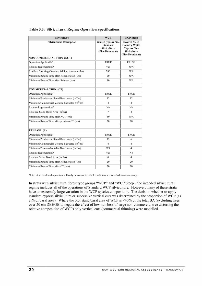
Table 3.3: Silvicultural Regime Operation Specifications
Silviculture WCP WCP SteepSilvicultural Description White Cypress Pine
StandardSilviculture
(Pine Dominant)
Inverell SteepCountry WhiteCypress PineSilviculture
(Pine Dominant)NON COMMERCIAL THIN (NCT)Operation Applicable? TRUE FALSE
Require Regeneration? Yes N/A
Residual Stocking Commercial Species (stems/ha) 280 N/A
Minimum Return Time after Regeneration (yrs) 20 N/A
Minimum Return Time after Release (yrs) 10 N/A
COMMERCIAL THIN (CT)Operation Applicable? TRUE TRUE
Minimum Pre-harvest Stand Basal Area (m2/ha) 12 12
Minimum Commercial Volume Extracted (m3/ha) 4 4
Require Regeneration? No No
Retained Stand Basal Area (m2/ha) 7 4
Minimum Return Time after NCT (yrs) 30 N/A
Minimum Return Time after previous CT (yrs) 20 20
RELEASE (R)Operation Applicable? TRUE TRUE
Minimum Pre-harvest Stand Basal Area (m2/ha) 12 6
Minimum Commercial Volume Extracted (m3/ha) 4 4
Minimum Pre-merchantable Basal Area (m2/ha) N/A 4
Require Regeneration? Yes No
Retained Stand Basal Area (m2/ha) 0 4
Minimum Return Time after Regeneration (yrs) 20 20
Minimum Return Time after CT (yrs) 20 20
Note: A silvicultural operation will only be conducted if all conditions are satisfied simultaneously.
In strata with silvicultural forest type groups “WCP” and “WCP Steep”, the intended silviculturalregime includes all of the operations of Standard WCP silviculture. However, many of these stratahave an extremely large variation in the WCP species composition. The decision whether to applystandard cypress silviculture or successive vertical cuts was determined by the proportion of WCP (asa % of basal area). Where the plot stand basal area of WCP is <40% of the total BA (excluding treesover 50 cm DBHOB to negate the effect of low numbers of large non-commercial tree distorting therelative composition of WCP) only vertical cuts (commercial thinning) were modelled.

30 N SW W EST ER N R EG IO N AL A SS ES S MEN T S – N AN D EW AR
3.6 LOG SPECIFICATIONS AND GRADES
Table 3.4: Western Regional Assessment Commercial Species Log Specifications
Log Type MinLength
(m)
MaxLength
(m)
MinSED(mm)
AcceptableQualities
Species
High Quality 2.6 14 120 AB WCP
Where:Stem Quality A = High QualityStem Quality B = Low QualityWCP = White Cypress Pine
Table 3.5: Description of Stem Quality Codes
MARVL InventoryQuality Codes Product General Log Grades
A High quality product quota sawlogs, small graded sawlogs, sleeper logs, veneer logs, larger poles, pilesand girders
B Low quality product salvage sawlogs, non-compulsory logs, small sawlogs
P Pulp pulp
W Waste stump, long butts, dockings
31 N SW W EST ER N R EG IO N AL A SS ES S MEN T S – N AN D EW AR
NATIVE FOREST STRATEGIC YIELD SCHEDULING
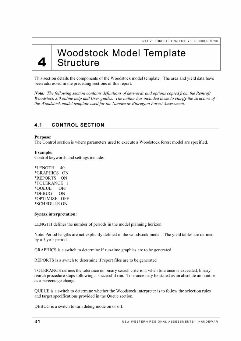
4Woodstock Model TemplateStructure
This section details the components of the Woodstock model template. The area and yield data havebeen addressed in the preceding sections of this report.
Note: The following section contains definitions of keywords and options copied from the RemsoftWoodstock 3.0 online help and User guides. The author has included these to clarify the structure ofthe Woodstock model template used for the Nandewar Bioregion Forest Assessment.
4.1 CONTROL SECTION
Purpose:The Control section is where parameters used to execute a Woodstock forest model are specified.
Example:Control keywords and settings include:
*LENGTH 40*GRAPHICS ON*REPORTS ON*TOLERANCE 1*QUEUE OFF*DEBUG ON*OPTIMIZE OFF*SCHEDULE ON
Syntax interpretation:
LENGTH defines the number of periods in the model planning horizon
Note: Period lengths are not explicitly defined in the woodstock model. The yield tables are definedby a 5 year period.
GRAPHICS is a switch to determine if run-time graphics are to be generated
REPORTS is a switch to determine if report files are to be generated
TOLERANCE defines the tolerance on binary search criterion; when tolerance is exceeded, binarysearch procedure stops following a successful run. Tolerance may be stated as an absolute amount oras a percentage change.
QUEUE is a switch to determine whether the Woodstock interpreter is to follow the selection rulesand target specifications provided in the Queue section.
DEBUG is a switch to turn debug mode on or off.
32 N SW W EST ER N R EG IO N AL A SS ES S MEN T S – N AN D EW AR
OPTIMIZE is a switch to determine if the Woodstock interpreter is to generate a LP matrix using theobjectives and constraints set in the Optimize section.
SCHEDULE is a switch to determine if the Woodstock interpreter is to follow a management scheduledefined in the Schedule section.
4.2 LIFESPAN SECTION
Purpose:The lifespan declaration indicates the maximum age a development type may reach before it isassumed to die or be replaced by another development type through succession.
A development type represents a parcel of forested land that is represented by a particular sequence oflandscape theme attributes. Development types are assumed to follow identical developmental patternsregardless of age. In a Woodstock model, a development type is defined by specifying the appropriatelandscape theme attributes and an associated age class distribution.
Example:Lifespan command used: ? ? ? ? ? ? ? ? ? ? 41
Syntax interpretation:The lifespan was set to an arbitrary period (41) in excess of the simulation period (40), to ensure themodel does not unexpectedly liquidate the forest resource before the end of the planning horizon.
? denotes that the command applies to all landscape theme attributes.
In this situation the lifespan command applies to the whole forest resource (all development types asindicated by ? ? ? ? ? ? ? ? ? ?)
4.3 AGGREGATE SECTION
Purpose:
AGGREGATE declares a set of actions that may be collectively used in the declaration of an output.
Example:
*AGGREGATE Aggr_DelayD0a D1a D2a D3a D4a D5a D6a D7a D8a D9a D10a
Syntax interpretation:
The new Landscape Aggregate is used to refer to all delay options in development type areastatements:
e.g. *A Nandewar Nandewar WCP 1 5 4 Western Standard RT1 D0a
This Aggr_Delay aggregate enables actions to be applied to all development types possessing D0a toD10a delays.

33 N SW W EST ER N R EG IO N AL A SS ES S MEN T S – N AN D EW AR
4.4 ACTIONS SECTION
Purpose:
The ACTIONS section provides the mechanism for implementing changes to development types in themodelled forest, such as to silvicultural interventions, natural catastrophic events or allocationdecisions. The outcomes of actions are specified in the TRANSITIONS section. The only inherentactivities Woodstock can perform are death and inventory growth, all others must be declared by theuser.
Example:
*ACTION delay0 N *OPERABLE delay0 ? ? ? ? ? ? ? ? ? Aggr_Delay _CP <= 1*ACTION delay1 N *OPERABLE delay1 ? ? ? ? ? ? ? ? ? Aggr_Delay _CP <= 1
*ACTION remove n harvest *OPERABLE remove;unavailable till period 1 ? ? ? ? ? ? ? ? ? D0 _CP >= 0 ? ? ? ? ? ? ? ? ? D1 _CP >= 0 ? ? ? ? ? ? ? ? ? D2 _CP >= 0 ? ? ? ? ? ? ? ? ? D3 _CP >= 0 ? ? ? ? ? ? ? ? ? D4 _CP >= 0 ? ? ? ? ? ? ? ? ? D5 _CP >= 0 ? ? ? ? ? ? ? ? ? D6 _CP >= 0 ? ? ? ? ? ? ? ? ? D7 _CP >= 0 ? ? ? ? ? ? ? ? ? D8 _CP >= 0 ? ? ? ? ? ? ? ? ? D9 _CP >= 0 ? ? ? ? ? ? ? ? ? D10 _CP >= 0
Syntax interpretation:
ACTION signals the beginning of a new action declaration.
OPERABLE signals the beginning of the operability declaration for an action.
CP is a system variable provided to allow the use of planning period as an operability criterion.

34 N SW W EST ER N R EG IO N AL A SS ES S MEN T S – N AN D EW AR
Delay actions:
delay0 is a user-declared action code or numberN or Y for default age reset.
? ? ? ? ? ? ? ? ? Aggr_Delay means this Action applies to all development types with a delay option inthe aggregate Aggr_Delay (this is all options)
_CP <=1 means action applicable in planning period <=1 i.e. Planning period 1, as planning periodsare from 1 – 20.
So collectively the command means that Action will apply to any development type, but it can onlyapply in period 1.
Remove actions:Remove means to harvest.N = no default age resetHarvest is description.
? ? ? ? ? ? ? ? ? D2 _CP >= 0 means any development type with a delay option 6 can be harvested inperiod after period 0 i.e. at any time during the planning horizon.
4.5 TRANSITIONS SECTION
Purpose:Transition declarations describe how the forest will respond to actions or events in terms of forestdevelopment.
Example:
*CASE delay10 *SOURCE ? ? ? ? ? ? ? ? ? ? *TARGET ? ? ? ? ? ? ? ? ? D10 100
*CASE remove*SOURCE ? ? ? ? ? ? ? ? ? D0 *TARGET ? ? ? ? ? ? ? ? ? D0 100 *SOURCE ? ? ? ? ? ? ? ? ? D1 *TARGET ? ? ? ? ? ? ? ? ? D1 100
*CASE _DEATH *SOURCE ? ? ? ? ? ? ? ? ? ? *TARGET ? ? ? ? ? ? ? ? ? ? 100

35 N SW W EST ER N R EG IO N AL A SS ES S MEN T S – N AN D EW AR
Syntax interpretation:
CASE signals the beginning of a transition declaration for an action. The corresponding action codefollows the CASE keyword
SOURCE indicates the source development types undergoing transition following the action given inthe previous *CASE statement.
TARGET indicates the target development types arising from the action given in the *CASE statementoccurring on the development types given in the previous *SOURCE statement
Delay transition
e.g.*CASE delay10*SOURCE ? ? ? ? ? ? ? ? ? ?*TARGET ? ? ? ? ? ? ? ? ? D10 100
This means any source development type can be allocated to the option of delay 10 periods. Thetarget only comprises 1 option, so up to 100% of all development types can be allocated this delay 10option.
Remove transition
e.g.*CASE remove*SOURCE ? ? ? ? ? ? ? ? ? D0*TARGET ? ? ? ? ? ? ? ? ? D0 100
This means that if the remove action is applied to the Delay 0 development types it will completelyremain in the same development type D0. This feature is used to model time dependent yield tables.Once a given delay option yield table is applied to a development type in period 1, then this same yieldtable applies for the duration. The remove command ensures the harvest yields are reported.
Death transitionA Woodstock system provided action that causes senescence.
4.6 OPTIMIZE SECTION
Purpose:
The OPTIMIZE section formulates the forest model as a linear program cf simulation model.In a linear programming (LP) model the user elects the objective, and the LP model determines thebest means of accomplishing that objective.

36 N SW W EST ER N R EG IO N AL A SS ES S MEN T S – N AN D EW AR
Example:
OPTIMIZE
*OBJECTIVE_MAX WCPVol 1.._LENGTH
*CONSTRAINTS
_EVEN(WCPVOL) 1.._LENGTH
;WCPVOL - 0.95 * WCPVOL[1] >= 0 2..40 ;Lower;WCPVOL - 1.05 * WCPVOL[1] <= 0 2..40 ;Upper
Syntax interpretation:
Objective keywordMAX indicates that objective function is to be maximised.
WCPVol is a user defined outputs. WCPVol is the total volume of White Cypress Pine sawlogs fromthe whole of the Sate Forest being modelled.
_LENGTH is the number of period in the planning horizon.
MAX WCPVol 1.._Length means the user wants the LP model to maximise the total volume ofWCP sawlogs to be produced form the estate over the whole planning horizon.
Constraints keyword
_EVEN(WCPVOL) 1.._LENGTH means the WCP volume must be even for the whole planninghorizon
WCPVOL - 0.95 * WCPVOL[1] >= 0 2 – 40 means the WCP sawlog volume in periods 2 - 40 mustbe within 95% of the period 1 volume
4.7 OUTPUTS SECTION
Purpose:
The OUTPUTS section describes how various benefits, costs and inventory measures are calculated.All outputs are triggered by actions and are usually a function of a per unit-area estimate in a yieldtable multiplied by the area treated using the triggering action. In some cases, outputs are simply by-products of a management regime.
37 N SW W EST ER N R EG IO N AL A SS ES S MEN T S – N AN D EW AR
Example:
OUTPUTS*OUTPUT WCPVol WCP HQL Total Volume Harvested*SOURCE remove HQ_Large_Yield_WCP
*OUTPUT NCTProp NCT Proportion*SOURCE remove NCT_Prop_Area
*OUTPUT CTProp Commercial Thin Proportion*SOURCE remove CT_Prop_Area
*OUTPUT RProp Release Poportion*SOURCE remove R_Prop_Area
*OUTPUT TPZ5_WCP WCP Volume harvested from Timber Price Zone 5 *SOURCE ? ? ? ? 5 ? ? ? ? ? remove HQ_Large_Yield_WCP
Syntax interpretation:
OUTPUT signals the beginning of a new output declaration
SOURCE indicates the action that triggers the output and the yield component used in the calculationof the output.
e.g.
*OUTPUT WCPVol WCP HQL Total Volume Harvested*SOURCE remove HQ_Large_Yield_WCP
This means that WCP Vol is the volume HQ_Large_Yield_WCP products defined in the yield tablewhich arise from the remove actions (harvesting).
e.g.*OUTPUT TPZ5_WCP WCP Volume harvested from Timber Price Zone 5 *SOURCE ? ? ? ? 5 ? ? ? ? ? remove HQ_Large_Yield_WCP
This means that TPZ_WCP is the volume HQ_Large_Yield_WCP products which arise from theremove actions (harvesting) in the development type TPZ5.
38 N SW W EST ER N R EG IO N AL A SS ES S MEN T S – N AN D EW AR
4.8 REPORTS SECTION
Purpose:The Reports section is where user defined reports about outputs are specified.
Example:
REPORTS
*TARGET C:\NAND\Scenarios\Basecase\Woodstock\Activity.dbf
_ACTIVITY 1.._LENGTH
*TARGET C:\NAND\Scenarios\Basecase\Woodstock\Results.wk1
WCPVol 1.._LENGTHTPZ5_WCP 1.._LENGTH
WCPVol 1.._LENGTHTPZ5_WCP 1.._LENGTH
Syntax interpretation:
TARGET indicates the destination for reports on outputs listed.
_ACTIVITY report is a system-provided report that details the outputs produced and developmenttypes treated by user-specified actions every period.
WCPVol 1.._LENGTH means the report will tabulate the total WCP Volume (output) for periods 1 tothe end of the planning horizon.
TPZ5_WCP 1.._LENGTH means the report will tabulate the WCP Volume for periods 1 to the end ofthe planning horizon which are sourced in TPZ5.
4.9 SCHEDULE SECTION
Purpose:
The SCHEDULE section is used to generate reports on an optimal solution found by an LP solver.After the LP solver software has found an optimal solution and created a solution file, the solution fileis processed to create a management schedule file.
Example:
SCHEDULE [Western.seq]
Syntax interpretation:

39 N SW W EST ER N R EG IO N AL A SS ES S MEN T S – N AN D EW AR
LP solution file is reported to *.seq file which details all actions implemented.e.g. content of SEQ file:
NANDEWAR NANDEWAR WCP 1 1 1 WESTERN STANDARD RT1 D0A 1 500.00 DELAY1 1 _EXISTING ;A54 11.5% of class
4.10 GRAPHICS SECTION
Purpose:
This command provides graphical displays of changes in the forest over time. These displays aregenerally for run-time use but they can be printed or copied and pasted into other Windowsapplications.
Example:
GRAPHICS*SCREENSIZE MAXIMIZED*WINDOW {3} ( 0, 0, 630, 998) "Harvest levels"_YAXIS(*,*,*)*LINES
WCPVol 1 1 _RED _SQUARE _SOLID "WCP Clearfell Vol"
TPZ5_WCP 1 _BLUE _SQUARE _DOTTED "Timber Price Zone 5"
Syntax interpretation:
Graph specifications are listed followed by the Output lines that appear on the chart.

40 N SW W EST ER N R EG IO N AL A SS ES S MEN T S – N AN D EW AR
NATIVE FOREST STRATEGIC YIELD SCHEDULING
5 Wood Supply Forecasting
5.1 MANAGEMENT OBJECTIVES AND CONSTRAINTS
Objective
The objective function of the Woodstock model run Base case is:
Maximise the volume of White Cypress Pine high quality sawlogs produced over the planning horizonof 200 years (Periods 1 to 40, where each period is 5 years). i.e. MAX WCPVol 1.._LENGTH
Planning horizon
Note: Period lengths are not explicitly defined in the Woodstock model. The yield tables are definedby 5-year period.
Constraints
An even flow constraint was set for the base case scenario. The volume harvested each year must notincrease or decrease from the preceding year.
i.e. _EVEN(WCPVol) 1.._LENGTH
Where:
EVEN = A Woodstock system function that generates even flow constraints for a givenoutput.
WCPVol is the target output – the volume of White Cypress Pine; 1 denotes the period.
1.. Length = from planning year 1 to the last planning year (40 periods)
Constraints – if we model current commitments.
(a) Wood supply commitments
In the Woodstock model, minimum production levels were set at the current commitment plus anadditional 5% to allow for the impact of Threatened Species Licence conditions. The 5% strike rate isa measure of the unmappable fauna and flora exclusions, which occur when harvesting operations arescheduled. This 5% loss of productive area is modelled by increasing the production target. (The areastatements could have been manually reduced by 5% and the actual allocation modelled.)

41 N SW W EST ER N R EG IO N AL A SS ES S MEN T S – N AN D EW AR
The woodstock model runs focussed on maximising the volume of high quality white cypress pinesawlogs over the planning horizon as this is the most valuable and primary product harvested from theNandewar forests.
(b) Regulating long term sustained yield
The wood supply target production level in the initial period production was set at the allocation levelto obtain forecasts of sustainable yield, percentage bounds (relational constraints) were used.
The level of production in each period may be constrained to within 5 of the original production levelof the target volume being maximised (WCPVol). For example:
WCPVOL - 0.95 * WCPVOL[1] >= 0 2..40WCPVOL - 1.05 * WCPVOL[1] >= 0 2..40
Where: WCPVOL[1] is the period 1 volume
(c) Wood supply constraints by Timber Price Zone (TPZ)
The forest resource is distributed widely across the Nandewar Bioregion and the demand nodes(industry locations) are also dispersed across the region. Consequently the wood is traditionallyallocated from specific supply zones (Timber Price Zones) to particular industries to minimise the costof haulage. Where supply deficits periodically arise, production from different zones is required sothat commitments can be met. This is not necessarily financially viable on a long-term basis.
Various options were modelled by Timber Price Zones for WCP, and for variable periods dependingon the term of wood supply contracts.
For example:
TPZ5_WCP >= ## 1.._LENGTHTPZ6_WCP >= ## 1..2
Where:TPZ_WCP is WCP production in Timber Price Zone (5 to 6),LENGTH is term of the planning horizon, ## is user defined volume.

42 N SW W EST ER N R EG IO N AL A SS ES S MEN T S – N AN D EW AR
5.2 MODELLING APPROACH
Various wood supply scenarios can may be modelled for alternative conservation reserve designs inthe Nandewar Bioregion, include:
n Modelling the maximum sustainable (non-declining) yield of White Cypress Pine (WCP) woodsupply (Base Case).
n Modelling total WCP wood supply commitments irrespective of proximity to demand nodesn Modelling WCP timber allocations by Timber Price Zonesn Modelling various production profiles reflecting possible industry rationalisation options
The Base Case wood supply forecast is included in the following section.

43 N SW W EST ER N R EG IO N AL A SS ES S MEN T S – N AN D EW AR
NATIVE FOREST STRATEGIC YIELD SCHEDULING
6 Base Case Wood Supply Forecast
6.1 SCENARIO
Base Case Scenario
Maximum sustainable supply of White Cypress Pine High Quality Sawlogs over 200 year planninghorizon
Subject to constraint that annual supply of White Cypress Pine High Quality Sawlogs must notincrease or decrease.
Table 6.1: Net Harvest Area
Stratum Timber PriceZone (TPZ)
TPZ no. TimberSupply Zone
(TSZ)
TSZ no. SilviculturalForest Type
Group
NHA (ha)
1 Gunnedah 5 Gunnedah 4 MIX 286.61 Gunnedah 5 Gunnedah 4 WCP 103.31 Gunnedah 5 Attunga 10 MIX 53.11 Gunnedah 5 Attunga 10 WCP 98.11 Inverell 6 Inverell 5 IBK 1,305.91 Inverell 6 Inverell 5 MIX 12,463.11 Inverell 6 Inverell 5 WCP 301.4
Sub Total 14,6112 Gunnedah 5 Gunnedah 4 MIX 34.12 Gunnedah 5 Gunnedah 4 WCP 9.92 Gunnedah 5 Attunga 10 MIX 21.42 Gunnedah 5 Attunga 10 WCP 28.32 Inverell 6 Inverell 5 IBK 26.92 Inverell 6 Inverell 5 MIX 3,709.72 Inverell 6 Inverell 5 WCP 81.7
Sub Total 3,912Total Area 18,523
§ NHA based on exclusion of Threatened Species Licence Stream Buffer widths.§ The net harvest area excludes the net harvest area modifier.

44 N SW W EST ER N R EG IO N AL A SS ES S MEN T S – N AN D EW AR
6.2 RESULTS
Figure 6.1: Forecast White Cypress Pine High Quality Sawlog Yield
Figure 6.2: Forecast White Cypress Pine High Quality Sawlog Yield – Timber Supply Zone

45 N SW W EST ER N R EG IO N AL A SS ES S MEN T S – N AN D EW AR
Figure 6.3: Annual Harvest Operation Area
Figure 6.4: Growing Stock – Volume by Species and Log Product
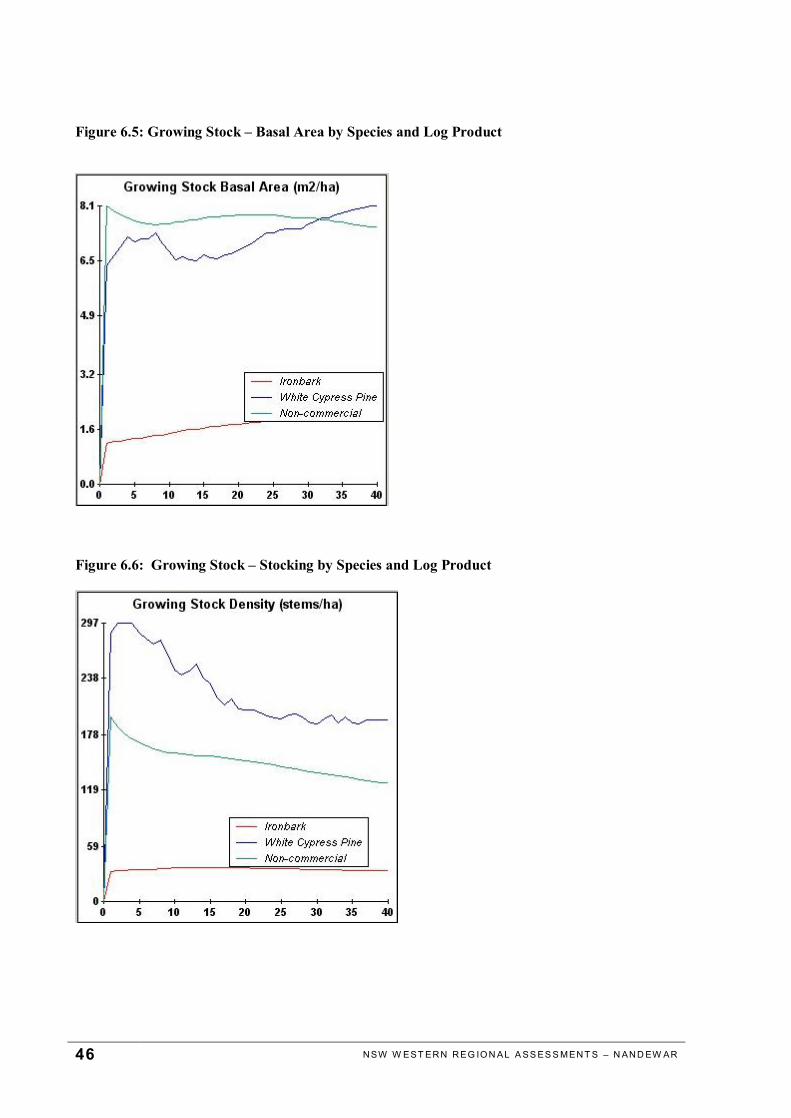
46 N SW W EST ER N R EG IO N AL A SS ES S MEN T S – N AN D EW AR
Figure 6.5: Growing Stock – Basal Area by Species and Log Product
Figure 6.6: Growing Stock – Stocking by Species and Log Product
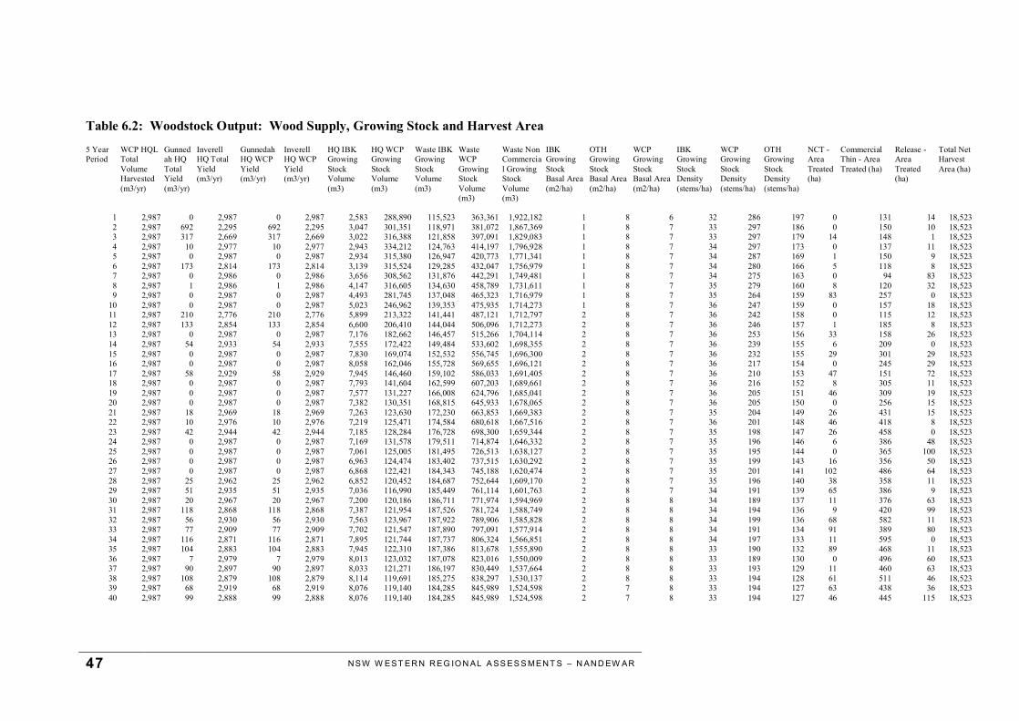
47 N SW W EST ER N R EG IO N AL A SS ES S MEN T S – N AN D EW AR
Table 6.2: Woodstock Output: Wood Supply, Growing Stock and Harvest Area5 YearPeriod
WCP HQLTotalVolumeHarvested(m3/yr)
Gunnedah HQTotalYield(m3/yr)
InverellHQ TotalYield(m3/yr)
GunnedahHQ WCPYield(m3/yr)
InverellHQ WCPYield(m3/yr)
HQ IBKGrowingStockVolume(m3)
HQ WCPGrowingStockVolume(m3)
Waste IBKGrowingStockVolume(m3)
WasteWCPGrowingStockVolume(m3)
Waste NonCommercial GrowingStockVolume(m3)
IBKGrowingStockBasal Area(m2/ha)
OTHGrowingStockBasal Area(m2/ha)
WCPGrowingStockBasal Area(m2/ha)
IBKGrowingStockDensity(stems/ha)
WCPGrowingStockDensity(stems/ha)
OTHGrowingStockDensity(stems/ha)
NCT -AreaTreated(ha)
CommercialThin - AreaTreated (ha)
Release -AreaTreated(ha)
Total NetHarvestArea (ha)
1 2,987 0 2,987 0 2,987 2,583 288,890 115,523 363,361 1,922,182 1 8 6 32 286 197 0 131 14 18,5232 2,987 692 2,295 692 2,295 3,047 301,351 118,971 381,072 1,867,369 1 8 7 33 297 186 0 150 10 18,5233 2,987 317 2,669 317 2,669 3,022 316,388 121,858 397,091 1,829,083 1 8 7 33 297 179 14 148 1 18,5234 2,987 10 2,977 10 2,977 2,943 334,212 124,763 414,197 1,796,928 1 8 7 34 297 173 0 137 11 18,5235 2,987 0 2,987 0 2,987 2,934 315,380 126,947 420,773 1,771,341 1 8 7 34 287 169 1 150 9 18,5236 2,987 173 2,814 173 2,814 3,139 315,524 129,285 432,047 1,756,979 1 8 7 34 280 166 5 118 8 18,5237 2,987 0 2,986 0 2,986 3,656 308,562 131,876 442,291 1,749,481 1 8 7 34 275 163 0 94 83 18,5238 2,987 1 2,986 1 2,986 4,147 316,605 134,630 458,789 1,731,611 1 8 7 35 279 160 8 120 32 18,5239 2,987 0 2,987 0 2,987 4,493 281,745 137,048 465,323 1,716,979 1 8 7 35 264 159 83 257 0 18,523
10 2,987 0 2,987 0 2,987 5,023 246,962 139,353 475,935 1,714,273 1 8 7 36 247 159 0 157 18 18,52311 2,987 210 2,776 210 2,776 5,899 213,322 141,441 487,121 1,712,797 2 8 7 36 242 158 0 115 12 18,52312 2,987 133 2,854 133 2,854 6,600 206,410 144,044 506,096 1,712,273 2 8 7 36 246 157 1 185 8 18,52313 2,987 0 2,987 0 2,987 7,176 182,662 146,457 515,266 1,704,114 2 8 7 36 253 156 33 158 26 18,52314 2,987 54 2,933 54 2,933 7,555 172,422 149,484 533,602 1,698,355 2 8 7 36 239 155 6 209 0 18,52315 2,987 0 2,987 0 2,987 7,830 169,074 152,532 556,745 1,696,300 2 8 7 36 232 155 29 301 29 18,52316 2,987 0 2,987 0 2,987 8,058 162,046 155,728 569,655 1,696,121 2 8 7 36 217 154 0 245 29 18,52317 2,987 58 2,929 58 2,929 7,945 146,460 159,102 586,033 1,691,405 2 8 7 36 210 153 47 151 72 18,52318 2,987 0 2,987 0 2,987 7,793 141,604 162,599 607,203 1,689,661 2 8 7 36 216 152 8 305 11 18,52319 2,987 0 2,987 0 2,987 7,577 131,227 166,008 624,796 1,685,041 2 8 7 36 205 151 46 309 19 18,52320 2,987 0 2,987 0 2,987 7,382 130,351 168,815 645,933 1,678,065 2 8 7 36 205 150 0 256 15 18,52321 2,987 18 2,969 18 2,969 7,263 123,630 172,230 663,853 1,669,383 2 8 7 35 204 149 26 431 15 18,52322 2,987 10 2,976 10 2,976 7,219 125,471 174,584 680,618 1,667,516 2 8 7 36 201 148 46 418 8 18,52323 2,987 42 2,944 42 2,944 7,185 128,284 176,728 698,300 1,659,344 2 8 7 35 198 147 26 458 0 18,52324 2,987 0 2,987 0 2,987 7,169 131,578 179,511 714,874 1,646,332 2 8 7 35 196 146 6 386 48 18,52325 2,987 0 2,987 0 2,987 7,061 125,005 181,495 726,513 1,638,127 2 8 7 35 195 144 0 365 100 18,52326 2,987 0 2,987 0 2,987 6,963 124,474 183,402 737,515 1,630,292 2 8 7 35 199 143 16 356 50 18,52327 2,987 0 2,987 0 2,987 6,868 122,421 184,343 745,188 1,620,474 2 8 7 35 201 141 102 486 64 18,52328 2,987 25 2,962 25 2,962 6,852 120,452 184,687 752,644 1,609,170 2 8 7 35 196 140 38 358 11 18,52329 2,987 51 2,935 51 2,935 7,036 116,990 185,449 761,114 1,601,763 2 8 7 34 191 139 65 386 9 18,52330 2,987 20 2,967 20 2,967 7,200 120,186 186,711 771,974 1,594,969 2 8 8 34 189 137 11 376 63 18,52331 2,987 118 2,868 118 2,868 7,387 121,954 187,526 781,724 1,588,749 2 8 8 34 194 136 9 420 99 18,52332 2,987 56 2,930 56 2,930 7,563 123,967 187,922 789,906 1,585,828 2 8 8 34 199 136 68 582 11 18,52333 2,987 77 2,909 77 2,909 7,702 121,547 187,890 797,091 1,577,914 2 8 8 34 191 134 91 389 80 18,52334 2,987 116 2,871 116 2,871 7,895 121,744 187,737 806,324 1,566,851 2 8 8 34 197 133 11 595 0 18,52335 2,987 104 2,883 104 2,883 7,945 122,310 187,386 813,678 1,555,890 2 8 8 33 190 132 89 468 11 18,52336 2,987 7 2,979 7 2,979 8,013 123,032 187,078 823,016 1,550,009 2 8 8 33 189 130 0 496 60 18,52337 2,987 90 2,897 90 2,897 8,033 121,271 186,197 830,449 1,537,664 2 8 8 33 193 129 11 460 63 18,52338 2,987 108 2,879 108 2,879 8,114 119,691 185,275 838,297 1,530,137 2 8 8 33 194 128 61 511 46 18,52339 2,987 68 2,919 68 2,919 8,076 119,140 184,285 845,989 1,524,598 2 7 8 33 194 127 63 438 36 18,52340 2,987 99 2,888 99 2,888 8,076 119,140 184,285 845,989 1,524,598 2 7 8 33 194 127 46 445 115 18,523
48 N SW W EST ER N R EG IO N AL A SS ES S MEN T S – N AN D EW AR
NATIVE FOREST STRATEGIC YIELD SCHEDULING
7 References
O’Gara, J. January 2004. Net Harvest Area Modifier. NSW Western Regional Assessments:Nandewar. Project Number: ####. Resource And Conservation Assessment Council. ## pp.
Turland, J.H. February 2004. Native Forest Growth and Yield Simulator. NSW Western RegionalAssessments: Nandewar. Project Number: NAND 08. Resource And Conservation AssessmentCouncil. 95 pp
Remsoft Inc. 2002a. Woodstock 3 modelling reference. Fredericton, Canada. 120pp.
Remsoft Inc. 2002b. Woodstock 3 users guide – Part 1. Fredericton, Canada. 156pp.
Remsoft Inc. 2002c. Woodstock 3 users guide – Part 2. Fredericton, Canada. 128pp.