nasa technical nasa tr r-459 report...t report no. 12. government accession no. nasa tr r-459 i 4....
TRANSCRIPT
NASA
=a,%
!
e_
z
TECHNICAL
REPORT
NASA TR R-459
DEFINING CONSTANTS, EQUATIONS,
AND ABBREVIATED TABLES OF
THE 1975 U.S. STANDARD ATMOSPHERE
R. A. 3.1illzJle_; C. A. RebeJ; L. G. Jacchia,
F. T. HmtJlg,, A. E. Cole, A. J. KatitoJ;
T.J. KeJieshea, S. P. Zimmermai!,
atid J. M. Forbes
Goddard Space Flight Cep, ter
Greetlbelt, Bid. 20771
_76 _91_
NATIONAL AERONAUTICS AND SPACE ADMINISTRATION • WASHINGTON, D. C. • MAY 1976
https://ntrs.nasa.gov/search.jsp?R=19760017709 2020-04-11T16:28:15+00:00Z

T Report No. 12. Government Accession No.NASA TR R-459 I
4. Title and Subtitle
Defining Constants, Equations, and Abbreviated Tables
of the 1975 U.S. Standard Atmosphere
7. Author(s)
R. A. Minzner et al.9. Performing Organization Name and Address
Goddard Space Flight Center
Greenbelt, Maryland 20771
12. Sponsoring Agency Name and Address
National Aeronautics and Space Administration
Washington, D.C. 20546
3. Recipient's Catalog No.
5. Report Date
M_v lq7R6. Per'_ormincj" Organization Code
9118. Performing Organization Report No.
G-7659|0. Work Unit No.
175-20-4011. Contract or Grant No.
13. Type of Report and Period Covered
Technical Report
14. Sponsoring Agency Code
15. Supplementary Notes
16. Abstract
The U.S. Standard Atmosphere, 1975 (COESA, 1975) is an idealized, steady-state repre-
sentation of the earth's atmosphere from the surface of the earth to 1000-km altitude, as
it is assumed to exist in a period of moderate solar activity. From 0 to 86 km, the atmo-
spheric model is specified in terms of the hydrostatic equilibrium of a perfect gas, with
that portion of the model from 0 to 51 geopotential kilometers (kln') being identical
with that of the U.S. Standard Atmosphere, 1962 (COESA, 1962). Between 51 and
86 km, the defining temperature-height profile has been modified from that of the
1962 Standard to lower temperatures between 51 and 69.33 km, and to greater values
between 69.33 and 86 kin. Above 86 kin, the model is defined in terms of quasi-
dynamic considerations involving the vertical component of the flux of molecules of
individual gas species. These conditions lead to the generation of independent number-
density distributions of the major species, N 2 , 02 , O, Ar, Ne, and H, consistent with
observations. The detailed definitions of the model are presented along with graphs
and abbreviated tables of the atmospheric properties of the 1975 Standard.
17. Key Words (Selected by Author(s))
Standard atmosphere, model, stratosphere
mesosphere, exosphere
Distribution Statement
Unclassified-Unlimited
19. Security Classif. (of this report) 20. Security Classif. (of this page) 21, No. of PagesUnclassified Unclassified 67
For sale by the National Technical Information Service, Springfield, Virginia 22161
CAT. 46
22. Price"$4.25


FOREWORD
Tables of the U.S. Standard Atmosphere to heights in excess of 300 km have appeared
in various editions over the past 18 years, the most recent being the U.S. Standard
Atmosphere, 1975 (COESA, 1975) to heights of 1000 km. These publications have
resulted from the work stimulated and guided by the Committee for Extension to
the Standard Atmosphere (COESA). This committee has a membership of about
30 organizations in government, industry, research institutions, and universities. The
particular organizational representations in COESA resulted primarily from either
the organization's scientific or administrative needs, or the organization's potential,
for contributions to a standard atmosphere. In several cases, however, an organiza-
tion's association with COESA stemmed largely from the interests and talents of
individual scientists employed by that organization.
During the course of this work, COESA was led by three co-chairmen, each associated
with one of the three principal sponsoring government agencies. These three agencies
and the co-chairmen were: National Aeronautics and Space Administration (NASA),
Maurice Dubin; National Oceanic and Atmospheric Administration (NOAA), Arnold
R. Hull; and United States Air Force (USAF), K. S. W. Champion.
The requirements and viewpoints of the many organizations participating in COESA
have shaped the format of the U.S. Standard Atmosphere, 1975 (COESA, 1975).
The scientific foundation for this Standard, however, is based upon the views of the
international comnmnity of scientists including, to a large extent, the members of
the Working Group of COESA. This Working Group, comprised of individual scien-
tists representing nearly all of the 30 organizations in the parent committee, has
based the U.S. Standard Atmosphere publication on current scientific and technical
knowledge, rather than on policy concerns.
The Working Group established five task groups for the preparation of the 1975
Standard; some members contributed to more than one task group. Each of these
task groups was charged with reviewing a particular category of available atmospheric
data, and with preparing recommendations for possible revisions of the U.S. Stan-
dard Atmosphere, 1962 (COESA, 1962). Three task groups (Task Groups I, II, and
III) dealt with data involving the three overlapping height regions: 50 to 100 km, 80
to 200 kin, and 140 to 1000 km, respectively. Task Group IV was charged with
combining the recommendations of Task Groups I, II, and III into an internally-con-
sistent model. Task Group V reviewed the present-day knowledge of minor con-
stituents.
111

The membership of each of the five task groups is listed in the Foreword of the U.S.
Standard Atmosphere, 1975 (COESA, 1975). This book also includes an extensive
section of detailed tables of the properties of the Standard, which applies to a mean,
midlatitude atmosphere for heights from 0 to 1000 km. The rationale for the model
and an extensive discussion of the minor atmospheric constituents are also included.
By contrast, Defining Constants, Equations, and Abbreviated Tables of the 1975
U.S. Standard Atmosphere emphasizes the definitions required to generate the tables
of atmospheric properties of the Standard. This report also contains an abbreviated
set of these tables, a set of graphs depicting the height profiles of these properties,
and a discussion of two properties not considered in the 1975 Standard, that is, geo-
potential pressure scale height and geopotential density scale height.
iv

CONTENTS
Page
ABSTRACT ............................ i
iiiFOREWORD ...........................
viiSYMBOLS ............................
1INTRODUCTION .........................
INTERNATIONAL SYSTEM OF UNITS ................ 2
BASIC ASSUMPTIONS AND FORMULAS ...............
2Adopted Constants ........................10Equilibrium Assumptions .....................13Gravity and Geopotential Altitude ..................
Mean Molecular Weight ...................... 16
Molecular-scale Temperature versus Geopotential Altitude
(0 to 84.3520 kin') ....................... 18
Kinetic Temperature versus Geometric Altitude (0 to 1000 kin) ....... 19
COMPUTATIONAL EQUATIONS ................. 22
23Pressure ............................
Number Density of Individual Species ................. 24
Mean Molecular Weight (Above 86 kin) ............... 29
Pressure and Mass Density (Above 86 kin) ............... 30
Total Number Density ....................... 30
Mass Density " . ........... 31
Mole Volume .......................... 31
Scale Heights .......................... 3135Mean Air-particle Speed ......................35Mean Free Path .........................36Mean Collision Frequency .....................37Speed of Sound .........................38Dynamic Viscosity ........................
CONTENTS(Continued)
COMPUTATIONAL EQUATIONS (continued)
Kinematic Viscosity ........ . ...............
Coefficient of Thermal Conductivity .................
SUMMARY OF TABULAR VALUES OF ATMOSPHERIC PROPERTIES ....
Sea-level Values .........................
Conversion of Metric to English Units .................
Tables of Atmospheric Properties ..................
ACKNOWLEDGMENTS .......................
REFERENCES ..........................
APPENDIX A-BOUNDARY-VALUE NUMBER DENSITIES OF
ATMOSPHERIC CONSTITUENTS ............
APPENDIX B-A SEGMENT OF AN ELLIPSE TO EXPRESS TEMPERATURE
VERSUS HEIGHT ...................
APPENDIX C-GEOPOTENTIAL AND MOLECULAR-SCALE
TEMPERATURE ...................
APPENDIX D-THE CALCULATION OF A DYNAMIC MODEL FOR THE
1975 U.S. STANDARD ATMOSPHERE ...........
Page
40
40
42
42
43
43
44
49
51
55
57
61
vi
SYMBOLS
a°1
A
A.
J
b.I
B.J
C.
J
CS
D.1
f(Z)
F.
!
F_!
One of the constant coefficients used to specify the elliptical segment of the
temperature-height profile, T(Z)
A set of species-dependent coefficients which, along with values of b i, are used to
define the set of height-dependent functions, D.1
Another constant coefficient used to specify the elliptical segment of T(Z)
A reaction-dependent rate coefficient used along with values Bj and Cj, to definek.
J
A dimensionless subscript designating a set of integers {0, 1,2, 3 ...} with 0
specifying sea-level conditions
A set of species-dependent exponents which, along with values of a i, are used to
define the set of height-dependent functions, Di
A dimensionless, reaction-dependent exponent used in the expression for kj
A reaction-dependent rate factor used as a part of all exponential expression in
the definition of k.l
The height-dependent speed of sound
The set of height-dependent, species-dependent, molecular-diffusion coefficients
for the atmospheric gas species O, 0 2 , Ar, He, and H
The hydrostatic term in the height-dependent expression for n i
The dimensionless, sea-level, fractional-volume concentration of the ith member
of the set of atmospheric gas species
The dimensionless, fractional-volume concentration of the ith member of the set
of atmospheric gas species adjusted for 86-kin height to account for the dissocia-
tion of O z
vii
g
?
go
H
Hp
?
Hp
HP
t
P
k
k.J
k t
K
L
LK,b
LM,b
M
The height-dependent acceleration of gravity (g(Z)) for 45 °
The adopted constant involved in the definition of the standard geopotential
meter, and in the relationship between geopotential height and geometric height
The geopotential height used as the argument for all tables up to 84.8520 kin'
(86 km)
The height-dependent, local pressure scale height of the mixture of gases com-
prising the atmosphere
The height-dependent, local geopotential pressure scale height of the mixture of
gases comprising tile atmosphere, and dependent upon the single variable, T M
The height-dependent, local density scale height of the mixture of gases com-
prising the atmosphere
The height-dependent, local geopotential density scale height of the mixture of
gases comprising the atmosphere
A dimensionless subscript designating the ith member of a set of gas species
A dimensionless subscript designating the jth member of a set of chemical reac-tions
Tile Boltzmann constant
The reaction rate of the jth chemical reaction
The height-dependent coefficient of thermal conductivity
The height-dependent, eddy-diffusion (or turbulent-diffusion) coefficient
The height-dependent, mean free path
A set of gradients of T with respect to Z
A set of gradients of TM with respect to H
The height-dependent, mean molecular weight of the mixture of gases constituting
the atmosphere
..°VIII
M.1
n,!
N
N A
P
P.I
qi
Qi
r o
R •
S
t
T
Tc
T M
Y_
U.!
The set of molecular weights of the several atmospheric gas species
The set of height-dependent number densities of the several atmospheric gas
species
The height-dependent, total number density of the mixture of neutral atmo-
spheric gas particles
The Avogadro constant
The height-dependent, total atmospheric pressure
The partial pressure of the ith gas species
One set of six adopted sets of species-dependent constants, that is, sets qi, Qi' ui'
Ui, wi, and Wi, all used in an empirical, species-dependent expression for the flux
term vi/(D i + K)
See qi
The adopted, effective earth's radius used to compute g(Z) for 45 ° North latitude,
and used for relating H and Z at that latitude
The universal gas constant
The Sutherland constant, used in computing
The height-dependent Celsius temperature
The height-dependent, Kelvin kinetic temperature, defined as a function of Z
for all heights above 86 kin, and derived from T M for heights below 86 km
The temperature coordinate of the center of the ellipse defining a portion of
T(Z)
The height-dependent, molecular-scale temperature defined as a function of H
for all heights from sea-level to 86 km
The exospheric temperature
See qi
ix

U°!
V.I
vm
V
W°I
W.1
Z
ZC
1
F
r/
P
o
See qi
The flow velocity of the ith gas species
The height-dependent mole volume
The height-dependent mean particle speed
See qi
See qi
Geometric height used as the argument of all tables at heights above 86 km
The height coordinate of the center of the ellipse defining a portion of T(Z)
The set of species-dependent, thermal-diffusion factors
A constant used for computing/a
A constant representing the ratio of specific heat at constant pressure to the
specific heat at constant volume used to define Cs
t
The ratio go/go
A dimensionless factor relating F i to FI
The height-dependent kinematic viscosity
A coefficient used to specify the exponential expression defining a portion of
T(Z)
The height-dependent coefficient of dynamic viscosity
The height-dependent mean collision frequency
A function of Z used in the exponential expression defining a portion of T(Z)
The height-dependent mass density of air
The effective mean collision diameter used in defining L and v
x
(I) G
_c
A height-dependent coefficient representing the reduced height of the atomic
hydrogen relative to a particular reference height, and used in the computation of
n(H) (number density of hydrogen)
The vertical flux of atomic hydrogen
The potential energy per unit mass of gravitational attraction
The potential energy per unit mass associated with centrifugal force
xi

DEFINING CONSTANTS, EQUATIONS, AND ABBREVIATED TABLES
OF THE 1975 U.S. STANDARD ATMOSPHERE
R. A. Minzner and C. A. Reber
Goddard Space Flight Center
L. G. Jacchia
Srnithsonian Astrophysical Observatory
F. T. Huang
Computer Science Corporation
A. E. Cole, A. J. Kantor, T. J. Keneshea,
S. P. Zimmerman, and J. M. Forbes
Air Force Cambridge Research Laboratories
INTRODUCTION
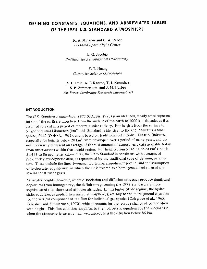
The U.S. Standard Atmosphere, 1975 (COESA, 1975) is an idealized, steady-state represen-
tation of the earth's atmosphere from the surface of the earth to 1000-km altitude, as it is
assumed to exist in a period of moderate solar activity. For heights from the surface to
51 geopotential kilometers (km'), this Standard is identical to the U.S. Standard Atmo-
sphere, 1962 (COESA, 1962), and is based on traditional definitions. These definitions,
especially for heights below 20 km', were developed over a period of many years, and do
not necessarily represent an average of the vast amount of atmospheric data available today
from observations within that height region. For heights from 51 to 84.8520 km' (that is,
51.413 to 86 geometric kilometers), the 1975 Standard is consistent with averages of
present-day atmospheric data, as represented by the traditional type of defining parame-
ters. These include the linearly-segmented temperature-height profile, and the assumption
of hydrostatic equilibrium, in which the air is treated as a homogeneous mixture of the
several constituent gases.
At greater heights, however, where dissociation and diffusion processes produce significant
departures from homogeneity, the definitions governing the 1975 Standard are more
sophisticated that those used at lower altitudes. In this high-altitude regime, the hydro-
static equation, as applied to a mixed atmosphere, gives way to the more general equation
for the vertical component of the flux for individual gas species (Colegrove et al., 1965;
Keneshea and Zimmerman, 1970), which accounts for the relative change of composition
with height. This flux equation simplifies to the hydrostatic equation for the special case
when the atmospheric gases remain well mixed, as is the situation below 86 km.

Thetemperature-heightprofilebetween86and 1000km is notexpressedasa seriesoflinearfunctions,asat loweraltitudes. Rather,it isdefinedin termsof four successivefunctionschosennot only to provideareasonableapproximationto observations,butalsoto yielda continuousfirst derivativewith respectto altitudeoverthe entireheightregime.
Observationaldataof variouskindsprovidethebasisfor independentlydeterminingvari-oussegmentsof this temperature-heightprofile. Theobservedtemperaturesat heightsbetween110and120kin wereparticularlyimportantin imposinglimits on theselectionof thetemperature-heightfunctionfor that region.At thesametime,theobserveddensi-tiesat 150km andabovestronglyinfluencedtheselectionof both thetemperatureandtheverticalextentof the low-temperatureisothermallayerimmediatelyabove86km.
Themeantemperaturesderivedfrom datasetsassociatedwith successiveheightregionswerenot necessarilycontinuous.In spiteof thissituation,it isnecessary,for purposesofcontinuityandof mathematicalreproducibilityof thetablesof this Standard,to expressthetemperaturein aseriesof consecutiveheightfunctionsfrom thesurfaceto 1000km.Theexpressionfor eachsuccessivefunctiondependsupontheend-pointvalueof thepre-cedingfunction,aswellasuponcertaintermsandcoefficientspeculiarto therelatedheightinterval. Thistotal temperature-heightprofileappliedto thefundamentalcontinuitymodels(that is,thehydrostaticequationandtheequationof motion),alongwith all theancillaryrequiredconstants,coefficients,andfunctions,definesthe U.S. Standard Atmo-
sphere, 1975 (COESA, 1975). The specification of this definition without any justification
in terms of observed data is the purpose of this document.
The definition of this Standard is completely consistent with the tables of two international
standard atmospheres, that of the International Civil Aviation Organization (ICAO, 1964)
defined up to 32-km altitude, and that of the International Organization for Standardiza-
tion (ISO, 1973) defined up to 50 kin.
INTERNATIONAL SYSTEM OF UNITS
The U.S. Standard Atmosphere, 1975 (COESA, 1975) is defined in terms of the Interna-
tional System (S.I.)of Units (Mechtley, 1973). A list of the symbols, names, and the
related quantities of the applicable basic and derived S.I. units, as well as of the three
non-standard metric units and one English unit employed in this Standard Atmosphere,
is presented in table 1.
BASIC ASSUMPTIONS AND FORMULAS
Adopted Constants
For purposes of computation, it is necessary to establish numerical values for various con-
stants appropriate to the earth's atmosphere. The adopted constants are grouped into
three categories. Category I includes those constants which are common to many branches
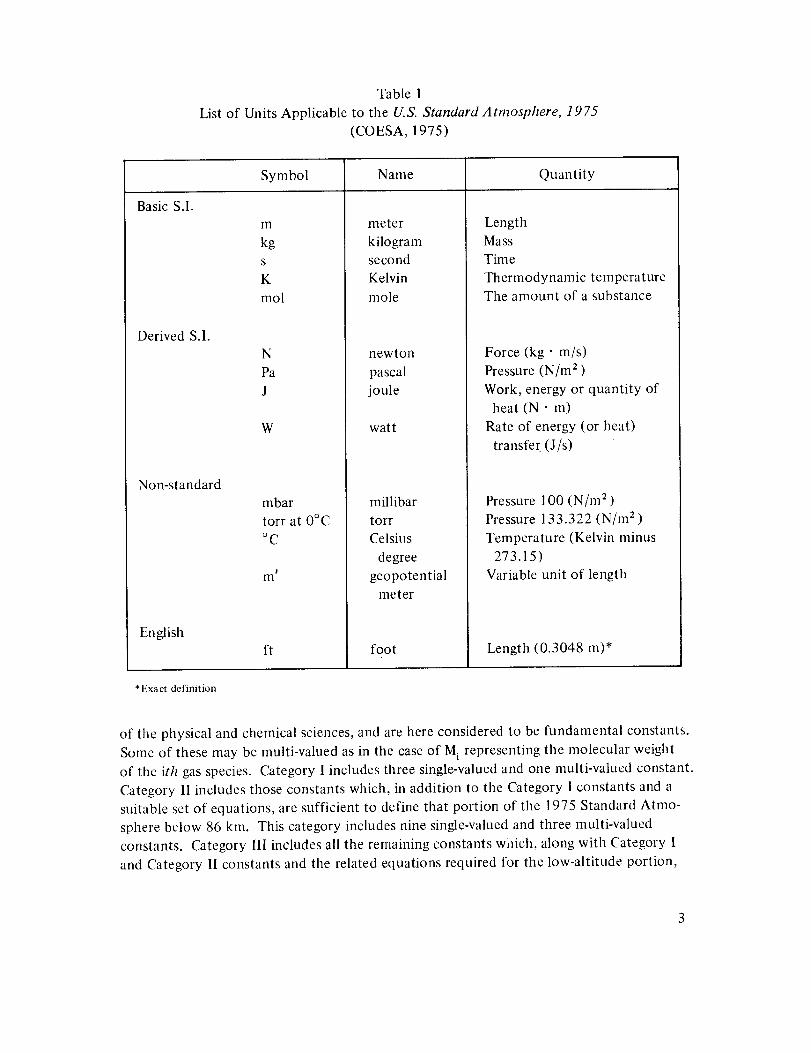
Table1Listof UnitsApplicableto the U.S. Standard Atrnosphere, 1975
(COESA, 1975)
Symbol Name Quantity
Basic S.I.
Derived S.I.
Non-standard
English
m
kg
S
K
tool
meter
kilogramsecond
Kelvin
mole
Length
Mass
Time
Thermodynamic temperature
The amount of a substance
N
Pa
l
W
mbar
torr at 0°C
°C
m P
ft
newton
pascal
joule
watt
millibar
torr
Celsius
degree
geopotential
meter
foot
Force (kg " m/s)
Pressure (N/m 2 )
Work, energy or quantity of
heat (N • m)
Rate of energy (or heat)
transfer. (J/s)
Pressure 100 (N/m 2 )
Pressure 133.322 (N/m 2)
Temperature (Kelvin minus
273.15)
Variable unit of length
Length (0.3048 m)*
*Exact definition
of the physical and chemical sciences, and are here considered to be fundamental constants.
Some of these may be multi-valued as in the case of Mi representing the molecular weight
of the ith gas species. Category I includes three single-valued and one nmlti-valued constant.
Category II includes those constants which, in addition to the Category I constants and a
suitable set of equations, are sufficient to define that portion of the 1975 Standard Atmo-
sphere below 86 kin. This category includes nine single-valued and three multi-valued
constants. Category llI includes all the remaining constants wifich, along with Category I
and Category II constants and the related equations required for the low-altitude portion,
3
plusanexpansionof that setof equations,arenecessaryto definethat portionof the 1975StandardAtmosphereabove86km. Thiscategoryincludes7 single-valuedand 12multi-valuedconstants.
Thevarioussingle-valuedandmulti-valuedconstantsarelistedalphabeticallyby symbolwith-in eachof thethreecategories.The discussion of each of these constants includes the nu-
merical value and dimensions, except that in the case of multi-valued constants, the values
are given in one or another of five tables immediately following the listing of the three
categories of constants.
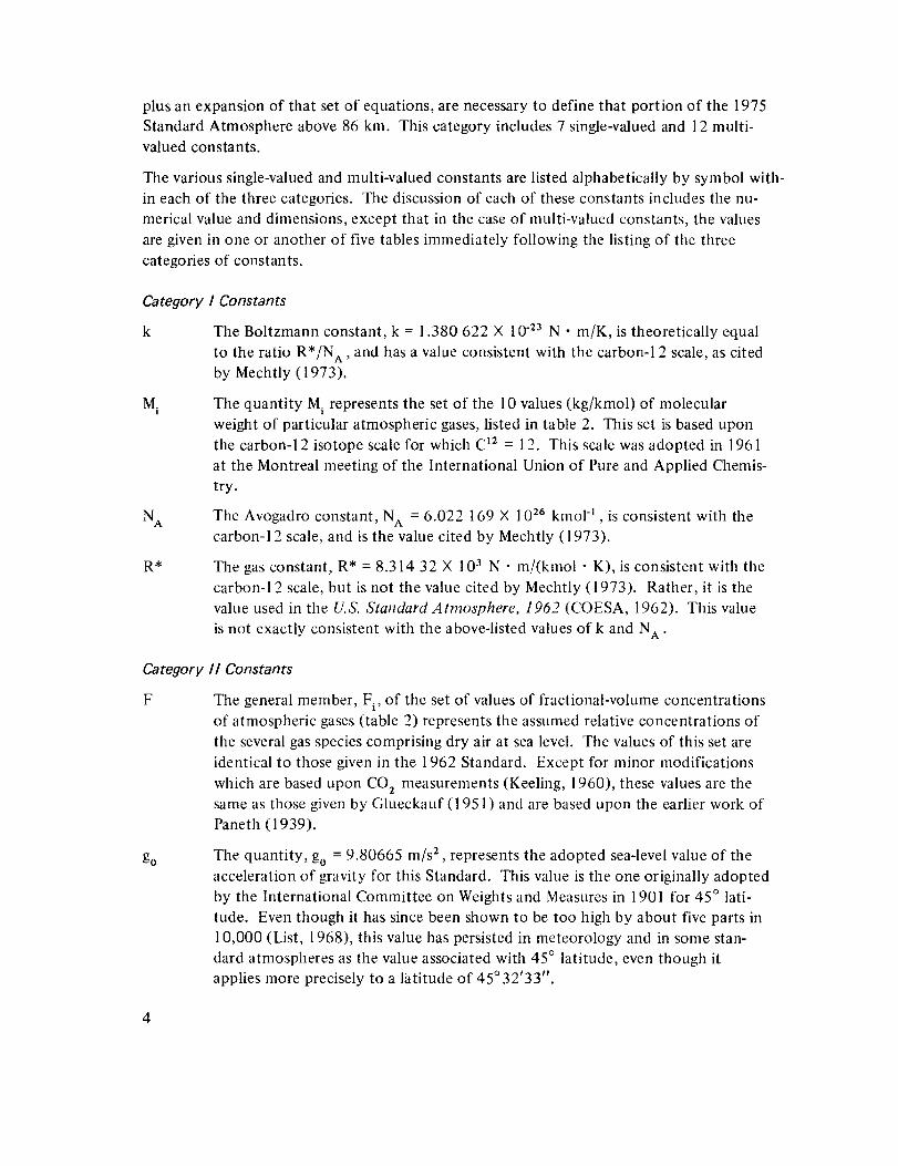
Category
k
M i
N A
R •
I Constants
The Boltzmann constant, k = 1.380 622 X 10-23 N - m/K, is theoretically equal
to the ratio R*/N A , and has a value consistent with the carbon-1 2 scale, as cited
by Mechtly (1973).
The quantity Mi represents the set of the 10 values (kg/kmol) of molecular
weight of particular atmospheric gases, listed in table 2. This set is based upon
the carbon-12 isotope scale for which C12 = 12. This scale was adopted in 1961
at the Montreal meeting of the International Union of Pure and Applied Chemis-
try.
The Avogadro constant, N A = 6.022 169 X 1026 kmol q , is consistent with the
carbon-I 2 scale, and is the value cited by Mechtly (1973).
The gas constant, R* = 8.314 32 X 103 N • m/(kmol • K), is consistent with the
carbon-12 scale, but is not the value cited by Mechtly (1973). Rather, it is the
value used in the U.S. Standard Atmosphere, 1962 (COESA, 1962). This value
is not exactly consistent with the above-listed values of k and N A .
Category
F
go
II Constants
The general member, Fi, of the set of values of fractional-volume concentrations
of atmospheric gases (table 2) represents the assumed relative concentrations of
the several gas species comprising dry air at sea level. The values of this set are
identical to those given in the 1962 Standard. Except for minor modifications
which are based upon CO 2 measurements (Keeling, 1960), these values are the
same as those given by Glueckauf (1951) and are based upon the earlier work of
Paneth (1939).
The quantity, go = 9.80665 m/s 2 , represents the adopted sea-level value of the
acceleration of gravity for this Standard. This value is the one originally adopted
by the International Committee on Weights and Measures in 1901 for 45 ° lati-
tude. Even though it has since been shown to be too high by about five parts in
10,000 (List, 1968), this value has persisted in meteorology and in some stan-
dard atmospheres as the value associated with 45 ° latitude, even though it
applies more precisely to a latitude of 45032'33 ''.
4
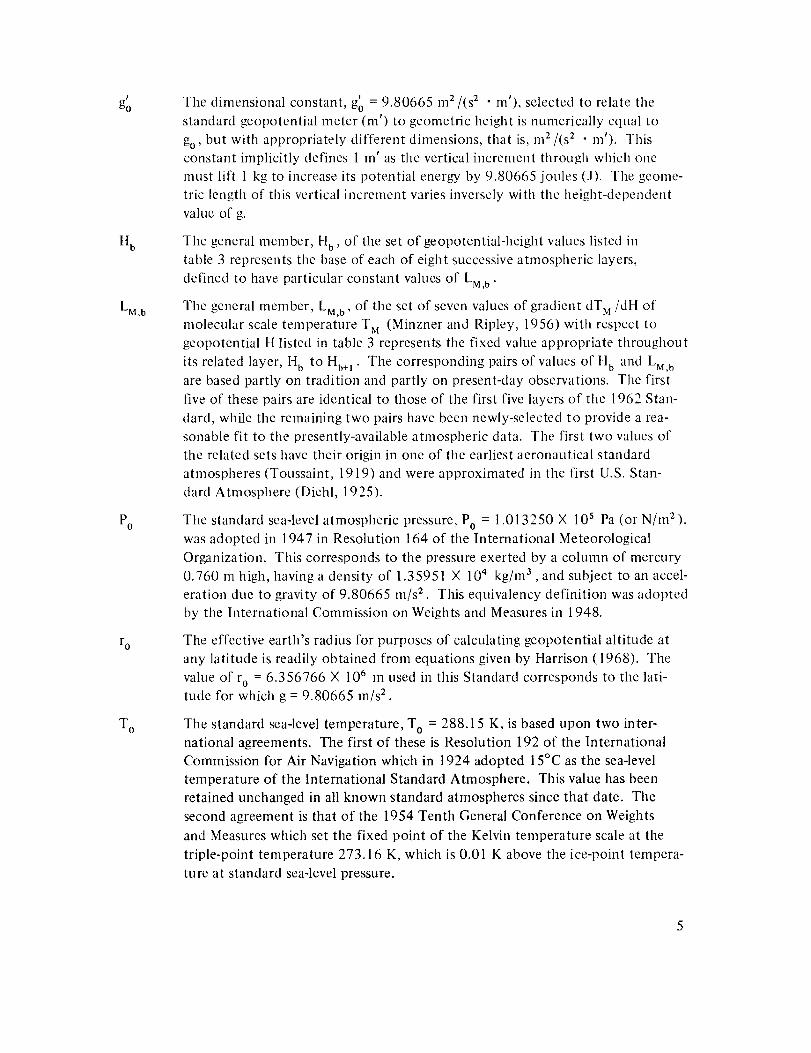
J
go
H b
LM ,b
P0
r o
T O
Tile dimensional constant, go = 9.80665 m 2/(s 2 • m'), selected to relate thestandard geopotential meter (m') to geometric height is numerically equal to
go, but with appropriately different dimensions, that is, m 2/(s 2 • m'). Thisconstant implicitly defines 1 m' as the vertical increment through which one
must lift 1 kg to increase its potential energy by 9.80665 joules (J). The geome-
tric length of this vertical increment varies inversely with the height-dependent
value of g.
The general member, Hb, of the set of geopotential-height values listed in
table 3 represents the base of each of eight successive atmospheric layers,
defined to have particular constant values of LM,b .
The general member, LM,b, of the set of seven values of gradient dT M/dH of
molecular scale temperature T M (Minzner and Ripley, 1956) with respect togeopotential H listed in table 3 represents the fixed value appropriate throughout
its related layer, H b to Hb+ 1 . The corresponding pairs of values of H b and LM,b
are based partly on tradition and partly on present-day observations. The first
five of these pairs are identical to those of the first five layers of the 1962 Stan-
dard, while the remaining two pairs have been newly-selected to provide a rea-
sonable fit to the presently-available atmospheric data. The first two values of
the related sets have their origin in one of the earliest aeronautical standard
atmospheres (Toussaint, 1919) and were approximated in the first U.S. Stan-
dard Atmosphere (Diehl, 1925).
The standard sea-level atmospheric pressure, P0 = 1.013250 X l0 s Pa (or N/m 2 ),
was adopted in 1947 in Resolution 164 of the International Meteorological
Organization. This corresponds to the pressure exerted by a column of mercury
0.760 m high, having a density of 1.35951 X 10⁴ kg/m 3, and subject to an accel-
eration due to gravity of 9.80665 m/s 2 . This equivalency definition was adopted
by the International Commission on Weights and Measures in 1948.
The effective earth's radius for purposes of calculating geopotentiai altitude at
any latitude is readily obtained from equations given by Harrison (1968). The
value of ro = 6.356766 X 10⁶ m used in this Standard corresponds to the lati-tude for which g = 9.80665 m/s 2.
The standard sea-level temperature, T o = 288.15 K, is based upon two inter-
national agreements. The first of these is Resolution 192 of the International
Commission for Air Navigation which in 1924 adopted 15°C as the sea-level
temperature of the International Standard Atmosphere. This value has been
retained unchanged in all known standard atmospheres since that date. The
second agreement is that of the 1954 Tenth General Conference on Weights
and Measures which set the fixed point of the Kelvin temperature scale at the
triple-point temperature 273.16 K, which is 0.01 K above the ice-point tempera-
ture at standard sea-level pressure.

3"
0
Category
a.I
b.1
K 7
Klo
The Sutherland constant, S = 110 K, (Hilsenrath et al., 1955) is a constant in
the empirical expression for dynamic viscosity.
The quantity/3 = 1.458 × 10⁶ kg/(s • m • K 1/2) (Hilsenrath et al., 1955) is a con-
stant in the expression for dynamic viscosity.
The ratio of specific heat of air at constant pressure to the specific heat of air
at constant volume is a dimensionless quantity with an adopted value 3' = 1.4.
This is the value adopted by the Aerological Commission of the International
Meteorological Organization in Toronto, 1948.
The mean effective collision diameter, o = 3.65 X 10 _° m, of gas molecules is a
quantity which varies with gas species and temperature. The adopted value is
assumed to apply in a dry, sea-level atmosphere. Above 85 kin, the validity of
the adopted value decreases with increasing altitude (Herschfelder et al., 1964;
Chapman and Cowling, 1960) due to the change in atmospheric composition.
For this reason, the number of significant figures in tabulations of quantities
involving o is reduced from that used for other tabulated quantities at heights
above 86 km.
III Constants
The quantity ai represents the general member of a set of five values (m -_ • S "1 )
of a species-dependent coefficient listed in table 4, and used in equation 8 for
designating the height-dependent, molecular-diffusion coefficient D. for theI
related gas species. (See b i.)
The quantity b i represents the general member of a set of five values (dimension-
less) of a species-dependent exponent listed in table 4, and used, along with the
corresponding value of a i, in equation 8 for designating the height-dependent,
molecular-diffusion coefficient for the related gas species. The particular values
of a i and b i adopted for this Standard have been selected to yield a height varia-
tion of D i consistent with observed number densities.
The quantity K 7 = 1.2 X 10² m2/s is the adopted value of the eddy-diffusion
coefficient K, at.Z 7 = 86 km, and in the height interval from 86 up to 91 kin.
Beginning at 91 km and extending up to 115 kin, the value of K is defined by
equation 7b. At 115 km the value of K equals Klo.
The quantity Klo = 0.0 m 2/s is the adopted value of the eddy-diffusion coeffi-
cient K at Z_o = 120 and throughout the height interval from 115 km through
1000 kin.

L_b
n(O) 7
n(H)ll
qi
Qi
Y 9
Y_
U i
U.1
The two-valued set of gradients LK, b = dT/dZ listed in table 5 was specifically
selected for this Standard to represent available observations. The first of these
two values of LK,b is associated with the layer 86 to 91 km, and the second with
the layer 110 to 120 kin.
The quantity n(O) 7 = 8.6 × 10 _6 m3 is the number density of atomic oxygen
assumed for this Standard to exist at Z 7 = 86 km. This value of atomic oxygen
number density, along with other defined constants, leads to particular values of
number density for N z , 02 , Ar, and He at 86 km. (See Appendix A.)
The quantity n(H)xl = 8.0 X 10 _° m -3 is the assumed number density of atomic
hydrogen at height Z_ = 500 km, and is used as the reference value in computing
the height profile of atomic hydrogen between 150 and 1000 km.
The quantity qi represents the first set of six sets of species-dependent coeffi-
cients listed in table 6 (that is, sets of qi, Qi' ui' Ui' wi' and Wi) the correspond-
hag members of all six of which are simultaneously used in an empirical expres-
sion for the vertical transport term vi/(D i + K) in the vertical flux equation for
the particular gas species. The species-dependent values of all six sets have been
selected for this Standard to adjust number-density profiles of the related gas
species to particular boundary conditions at 150 and 450 kin, as well as at 97 km
in the case of atomic oxygen. These boundary conditions all represent observed
or assumed average conditions. (See equation 37.)
The quantity Qi represents the second set of the six sets of constants described
along with qi above, and listed in table 6.
The quantity T 9 = 240 K represents the kinetic temperature at Z 9 = 110 km.
This temperature has been adopted along with the gradient LK,9 = 12 K/kin to
generate a linear segment of T(Z) for this Standard between 110 and 120 km.
The quantity T = 1000 K represents the exospheric temperature, that is, the
asymptote which the exponential function, representing T(Z) above 120 kin,
closely approaches at heights above about 500 kin, where the mean free path
exceeds the scale height. The value ofT adopted for this Standard is assumed
to represent mean solar conditions.
The quantity ui represents the third set of the six sets of constants described
along with qi above, and listed in table 6.
The quantity U i represents the fourth set of the six sets of constants described
along with qi above, and listed in table 6.

W°!
W.1
Z b
I
The quantity wi represents the fifth set of the six sets of constants described
along with qi above, and listed in table 6.
The quantity Wi represents the sixth set of the six sets of constants described
along with qi above, and listed in table 6.
The quantity Z b represents a set of six values of Z for b equal to 7 through 12.
The values Z 7 , Z 8 , Z 9 , and Z10 correspond respectively, to the base of succes-
sive layers characterized by successive segments of the adopted temperature-
height function for this Standard. The fifth value, ZI_, is the reference height
for the atomic hydrogen calculation, while the sixth value, Z12, represents the
top of the region for which the tabular values of the Standard are given. These
six values of Z b , along with the designation of the type of temperature-heightfunction associated with the first four of these values, plus the related value of
LK,b , for the two segments having a linear temperature-height function, arelisted in table 5.
The quantity 0q represents a set of six adopted species-dependent, thermal-diffu-sion coefficients listed in table 4.
The quantity _ = 7.2 × 101_ m 2 • s-_ for the vertical flux is chosen as a com-
promise between the classical Jeans' escape flux for To = 1000 K, with correc-
tions to take into account deviations from a Maxwellian velocity distribution at
the critical level (Brinkman, 1971) and the effects of charge exchange with tI +
and O + in the plasmasphere (Tinsley, 1973).
Table 2
Molecular Weights and Assumed Fractional-volume Composition of Sea-level Dry Air
Gas Species
N 2
0 2Ar
('0 2Ne
tie
Kr
Xe
CH 4
H2
Molecular Weight
Mi (kg/knlol)
28.013 4
31.998 8
39.948
44.009 95
20.183
4.002 6
83.80
131.30
16.043 03
2.015 94
Fractional Volume
Fi (dimensionless)
0.780 84
0.209 476
0.009 34
0.000 314
0.000018 18
0.000 005 24
0.000001 14
0.000 000 087
0.000 002
0.000 000 5
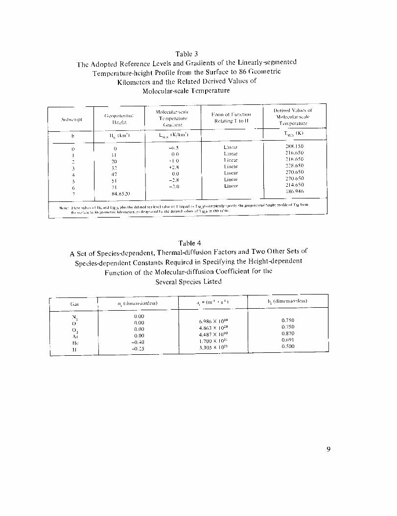
Table 3
The Adopted Reference Levels and Gradients of the Linearly-segmented
Temperature-height Profile from the Surface to 86 GeometricKilometers and the Related Derived Values of
Molecular-scale Temperature
Molccular-scalc Derived Values ofForm of Function Molecular-scale
(;eopotcntial .fcml_craturc Relating T to IISubscript tleight (;radient Temperature
h t11, (km'} LM.h (K/'km't TM._ (K)
0
I1
20
32
47
51
71
84.8520
-6.5
0.0
+1.0
+2.8
0.0
-2.8
-2.0
Linear
Linear
Linear
Linear
Linear
Linear
Linear
288.150
216,650
216.650
228.650
270.650
270.650
214.650
186.946
Note: 1 hese values of II b anti L M,b plus Ihe defined sea-level va e of T equal to FM, 01 completely specify the geolx_tential-heighI profile of T M from
',he surface to g6 geotnctric kilometers, as designaled b3, tile derived values of FM, b in Ihis table.
Table 4
A Set of Species-dependent, Thermal-diffusion Factors and Two Other Sets of
Species-dependent Constants Required in Specifying the Height-dependent
Function of the Molecular-diffusion Coefficient for the
Several Species Listed
[;as a i(dimensionless) a i =(ml .stl b i(dimensonless
S 2
O
()2Ar
tte
It
0.00
0.00
0.00
0.00
-0.40
-0.25
6.986 X 10²°
4.863 X 10²°
4.487 X I02°
1.700 X 10²¹
3.305 × 10²t
0.750
0.750
0.870
0.691
0.500
9

Table5TheConstantsandFunctionsAdoptedto DefinetheFour-layerTemperature-heightProfilefor AltitudesBetween86and1000km,PlustheDerivedTemperaturesat the
BoundaryHeightsof theSeveralLayers
Subscript
7
8
9
10
I1
12
(;comctric
llcight
Z b (kin)
86
9 I
I10
120
500
1000
Kinetic-temperature
(;radicnl
L_... (K/kin)
0.0
12.0
I:Ol'lll of [:tlllction
Relating T to Z
Linear
Elliptical
Linear
l_ixponcntial
Derived Kinetic
Temperature
T (K)
186.87
186.87
360.00
999.24
1000,00
Nole: These adopted specifications, including Ihc adopted kinelic temperature, 2411 K at I I0 kin, and the kinelic temperature, 186.87 K derived from T M
at 86 kin, plus Ihe speti(lt form ol the c xponential function, cqualiun 31, and the requirement that dl/d Z be continuous 110111 Z 86 kin to Z -
10011 kin. define the height prul]le ol F bci wcen these height limils. The specific form ol tile ellipse, cqualion 27 which satisfies the ,,cveral adopted
condilions is derived in Appemli_. B.
Table 6
Values of Six Sets of Species-dependent Coefficients Applicable to the Empirical
Expression Representing the Flux Term vi/(D i + K) in the Equation forNumber Density of the Four Species Listed
Gas qi (kin3)
O -3.416248 X 10 .3*
O= 0Ar 0
tic 0
Oi (k111"3)
-5.809644 X IO4
1.3(_6212X 104
9.434079 X 10⁴
-2.457369 X IO4
u i (kin)
97.0
Ui (kin)
56.00311
86.000
86.000
86.000
Wi (kin 3 )
5.008765 X 10⁴
W i (kin -3 )
2.706240 × 10 s
8.333333 × 10 "s
8.333333 × l ff s
6.666667 × 10 _
*'l'his_ ueo[qi pp es_myh_r86,cZ<97knl. I't_rZ >97km, qi=O.Okin-3.
Equilibrium Assumptions
The air is assumed to be ctry, and at heights sufficiently below 86 kin, the atmosphere is
assumed to be homogeneously mixed with a relative-volume composition leading to a con-
stant mean molecular weight, M. In this height region of complete mixing, the air is
treated as if it were a perfect gas, and the total pressure P, the temperature T, and the total
density/9 at any point in the atmosphere are related by the equation of state, that is, the
perfect gas law, one form of which is
p-R*'T
P - (1)M
10
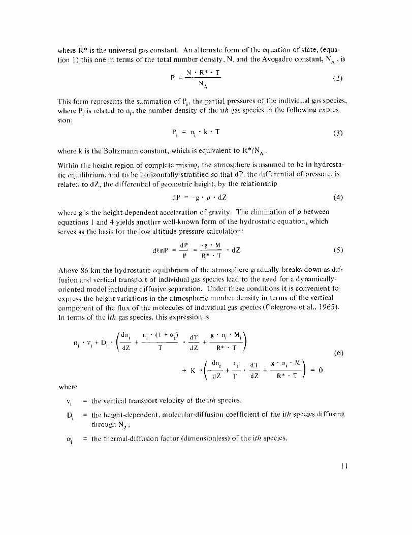
where R* is the universal gas constant. An alternate form of the equation of state, (equa-
tion 1) this one in terms of the total number density, N, and the Avogadro constant, N A , is
N.R*-TP - (2)
N A
This form represents the summation of Pi, the partial pressures of the individual gas species,
where Pi is related to n i, the number density of the ith gas species in the following expres-sion:
Pi = ni " k • T (3)
where k is the Boltzmann constant, which is equivalent to R*/N A .
Within the height region of complete mixing, tile atmosphere is assumed to be in hydrosta-
tic equilibrium, and to be horizontally stratified so that dP, the differential of pressure, is
related to dZ, the differential of geometric height, by the relationship
dP = -g.p • dZ (4)
where g is the height-dependent acceleration of gravity. The elimination of 0 between
equations 1 and 4 yields another well-known form of the hydrostatic equation, which
serves as the basis for the low-altitude pressure calculation:
dP -g. Md_nP ..... dZ (5)
P R* • T
Above 86 km the hydrostatic equilibrium of the atmosphere gradually breaks down as dif-
fusion and vertical transport of individual gas species lead to the need for a dynamically-
oriented model including diffusive separation. Under these conditions it is convenient to
express the heigilt variations in the atmospheric number density in terms of the vertical
component of the flux of the molecules of individual gas species (Colegrove et al., 1965).
In terms of the ith gas species, this expression is
(dn i n i • (l + oei} dT g22i" Mi./ni " vi+ Di " \ dZ + +T dZ R* • T l
where
dni ni dT g" n i • M)+ K " _+I.__+ R*--" = 0dZ T dZ T
(6)
V.1
D i
!
= the vertical transport velocity of the ith species,
= the height-dependent, molecular-diffusion coefficient of the ith species diffusing
through N 2 ,
= the thermal-diffusion factor (dimensionless) of the ith species,
11

Mi = the molecular weight of the ith species,
M = the molecular weight of the gas through which the ith species is diffusing, and
K = the height-dependent, eddy-diffusion coefficient.
The function K is defined differently in each of three height regions
1. For 86 _< Z <; 95 km,
K = K 7 = 1.2 X 10² m 2/s (7a)
2. For95 _<Z< 115 km,
K =
3. For l15_<Z<1000,
400K 7 • exp 1 - 400- (Z- 9512
(7b)
K = K10 = 0.0m2/s (7c)
The function D i is defined by
b.
aiI) i (8)
)2n i
where a i and bi are the species-dependent constants defined in table 4, while T and Zn i are
both altitude-dependent quantities which are specified in detail below. The values of Di,
determined from these altitude-dependent quantities, and the defined constants ai and bi
are plotted in figure 1 as a function of altitude for each of four species, O, O z , Ar, and He.
E
¢._
.9,(O
150 F T T r , - - =. _o,_co_ _.FFos,o. '/////, op ////...o! o. us,o.
loot-
F JJ// i80L ± _ a ,
10 0 1O 1 10 2 10 3 10 4 10 5
MOLECULAR-DIFFUSION AND EDDY-DIFFUSION COEFFICIENTS,m_'/s
Figure 1. Molecular-diffusion and eddy-diffusion coefficients versus geometric altitude.
12

The value of D i for atomic hydrogen, H, for heights just below 150 km is also shown in
figure 1. This same figure contains a graph of K as a function of altitude. It is apparent
that for heights sufficiently below 90 km, values of D i are negligible compared with K,
while above 115 km, the reverse is true. In addition, it is known that the flux velocity, vi,
for the various species becomes negligibly small at altitudes sufficiently below 90 kin.
The information regarding the relative magnitudes of vi, Di, and K permits us to consider
the application of equation 6 in each of several regimes. One of these regimes is for
heights sufficiently below 90 km, such that v i and D i are both extremely small compared
with K. Under these conditions, equation 6 reduces to the following form of the hydro-
static equation:
dni dT -g" M__ + .... dZ (9)
n. T R* " T1
Since the left-hand side of this equation is seen through equation 3 to be equal to dPi/Pi,
equation 9 is seen to be the single-gas equivalent to equation 5. Consequently, while equa-
tion 6 was designed to describe the assumed equilibrium conditions of individual gases
above 86 kin, it is apparent that it also describes such conditions below that altitude. Here
the partial pressure of each gas comprising the total pressure varies in accordance with the
mean molecular weight of the mixture, as well as in accordance with the temperature and
the acceleration of gravity. Nevertheless, equation 5, expressing total pressure, represents
a convenient step in the development of equations for computing total pressure versus geo-
metric height, when suitable functions are introduced to account for the altitude variation
in T, M, and g.
It has been customary in standard-atmosphere calculations to effectively eliminate the
variable portion of the acceleration of gravity from equation 5 by the transformation of
the independent variable Z to geopotential altitude H. This simplifies both the integration
of equation 5 and the resulting expression for computing pressure. The relationship be-
tween geometric and geopotential altitude depends upon the concept of gravity.
Gravity and Geopotential Altitude
Viewed in the ordinary manner from a frame of reference fixed in the earth, the atmosphere
is subject to the force of gravity. The force of gravity is the resultant (vector sum) of two
forces: (1) the gravitational attraction in accordance with Newton's universal law of gravi-
tation, and (2) the centrifugal force, which results from the choice of an earthbound, rota-
ting frame of reference.
The gravity field, being a conservative field, can be derived conveniently from the gravity
potential energy per unit mass, that is, from the geopotential q_. This is given by
= _c + _c (1 O)
13

whereeecis thepotentialenergyperunit massof gravitationalattraction,andeecis thepotentialenergyperunit massassociatedwith thecentrifugalforce. Thegravityperunitmassis
g = Vee (1l)
whereVeeis thegradient(ascendant)of thegeopotential.Theaccelerationdueto gravityisdenotedby gandisdefinedasthemagnitudeof g,that is,
g =lgl = IVeel (12)
When moving along an external normal from any point on the surface eel to a point on the
surface ee2 infinitely close to the first surface, so that ee2 = ee_ + dee, the incremental work
performed by shifting a unit mass from the first surface to the second will be
hence
d+ = g ' dZ (13)
Zee = g "dZ. (14)
Tile unit of measurement of geopotential (Appendix C) is the standard geopotential meter
which represents the work done by lifting a unit mass one geometric meter, through a
region in which the acceleration of gravity is uniformly 9.80665 m/s 2 .
The geopotential of any point with respect to mean sea level (assumed zero potential),
expressed in geopotential meters, is called geopotential altitude. Therefore, geopotential
altitude, H, is given by
l f0 ZH ..... g • dZ (15)t t
go go?
and is expressed in geopotential meters (m') when the unit geopotential, go, is set equal to
9.80665 m2/(s 2 • m').
With geopotential altitude defined as in equation 15, the differential of equation 15 may
be expressed as
t
go " dH = g • dZ. (16)
This expression, introduced into equation 5, will reduce the number of variables prior to
its integration, thereby leading to an expression for computing pressure as a function of
geopotential height.
The inverse-square law of gravitation provides an expression for g as a function of altitude
with sufficient accuracy for most model-atmosphere computations:
14
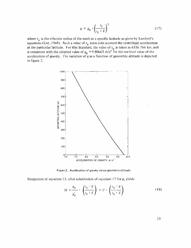
(17)
wherero is theeffectiveradiusof the earth at a specific latitude as given by Lambert's
equations (List, 1968). Such a value of ro takes into account the centrifugal acceleration
at the particular latitude. For this Standard, the value of ro is taken as 6356.766 kin, and
is consistent with the adopted value of go = 9.80665 m/s 2 for the sea-level value of theacceleration of gravity. The variation of g as a function of geometric altitude is depicted
in figure 2.
900
800
700
w" 600
500<
400
23OO
200
100
07.0 7.5 8.0 8.5 9.0 9.5 10.0
ACCELERATION OF GRAVITY, m/s 2
Figure 2. Acceleration of gravity versusgeometric altitude.
Integration of equation 15, after substitution of equation 17 for g, yields
(r0Z)H .... I''
go _ r° + Z ] ro + Z
(18)
15

or
r0 • Hz - (19)
P'r0-H
where P = go/g'o = 1 m'/m.
Differences between geopotential altitudes obtained from equation 18 for various values
of Z, and those computed from the more complex relationship used in developing the
U.S. Standard Atmosphere, 1962, (COESA, 1962) are small. For example, values of H
computed from equation 18 are approximately 0.2, 0.4, and 33.3 m greater at 90, 120,
and 700 km, respectively, than those obtained from the relationship used in the 1962
Standard. In the 1975 Standard, geopotential altitude is used explicitly only at heights
below 86 geometric kilometers.
The transformation from Z to H (equation 16) in the development of the pressure-height
relationship, for heights between the surface of the earth and 86-kin altitude, makes it
necessary to define the altitude variation of T and M in terms of H. It is convenient, there-
fore, to determine the sea-level value of M, as well as the extent of any height dependence
of this quantity, between the surface of the earth and 86-km altitude. Then, for this low-
altitude regime, the two variables, T and M, are combined with the constant Mo into a
single variable T M , which is then defined as a function of H.
Mean Molecular Weight
The mean molecular weight, M, of a mixture of gases is by definition
Z(n i " M i)M - (20)
Zn i
where n i and M i are the number density and defined molecular weight, respectively, of the
ith gas species. In that part of the atmosphere, between the surface of the earth and about
80-km altitude, mixing is dominant, and the effect of diffusion and photochemical proces-
ses upon M is negligible. In this region, the fractional composition of each species is as-
sumed to remain constant at the defined value, Fi, and M remains constant at its sea-level
value, M0. For these conditions, n i is equal to the product of Fi times the total numberdensity, N, so that equation 20 may be rewritten as
[F i • N(Z)" Mi] Z(Fi • Mi)
M = M0 = - (21)£[F i • N(Z)] ZF i
The right-hand element of this equation results from the process of factoring N(Z) out of
each term of both the numerator and the denominator of the preceding fraction, so that,
in spite of the altitude dependence of N, M is seen analytically to equal M o over the entire
altitude region of complete mixing. When the defined values of F i and M i (from table 2)
16
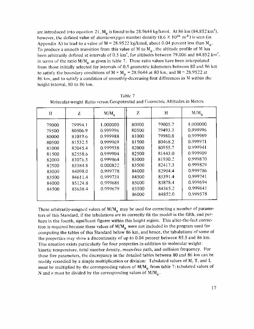
areintroducedinto equation21,M0isfoundto be28.9644kg/kmol. At 86km(84.852km'),however,thedefinedvalueof atomic-oxygennumberdensity(8.6 × 10¹⁶m3 ) isseen(inAppendixA) to leadto avalueof M = 28.9522kg/kmol,about0.04percentlessthanMo.To produceasmoothtransitionfrom thisvalueof M to Mo, the altitudeprofileof M hasbeenarbitrarilydefinedat intervalsof 0.5kin', for altitudesbetween79.006and84.852km',in termsof theratioM/M0 asgivenin table7. Theseratiovalueshavebeeninterpolatedfrom thoseinitially selectedfor intervalsof 0.5geometrickilometersbetween80and86klnto satisfytheboundaryconditionsofM = Mo = 28.9644at 80kin, andM = 28.9522at86km,andto satisfyaconditionof smoothly-decreasingfirst differencesin M within theheightintelwal,80 to 86kin.
Table7Molecular-weightRatioversusGeopotentialandGeometricAltitudesill Meters
H Z M/Mo Z H M/Mo
790007950080000805008100081500820008250083000835008400084500
79994.180506.981019.681532.582045.482558.683071.583584.884098.084611.485124.885638.4
1.0000000.9999960.9999880.9999690.9999380.9999040.9998640.0008220.9997780.9997310.9996810.999679
80000805008100081500820008250083000835008400084500850008550086000
79005.779493.379980.880468.280955.781443.081930.282417.382904.483391.483878.484365.284852.0
1.0000000.9999960.9999890.9999710.9999410.9999090.9998700.9998290.9997860.9997410.9996940.9996410.999578
Thesearbitrarily-assignedvaluesof M/M0 maybeusedfor correctinganumberof parame-tersof thisStandard,if thetabulationsareto correctlyfit themodelin the fifth, andper-hapsin thefourth, significantfigureswithin thisheightregion.Thisafter-the-factcorrec-tion isrequiredbecausethesevaluesof M/Mo werenot includedin theprogramusedforcomputingthetablesof this Standardbelow86kin,andhence,thetabulationsof someofthepropertiesmayshowadiscontinuityof up to 0.04percentbetween85.5and86km.Thissituationexistsparticularlyfor fourpropertiesinadditionto molecularweight:kinetictemperature,total numberdensity,mean-freepath,andcollisionfrequency.Forthesefiveparameters,thediscrepancyin the detailedtablesbetween80and86kmcanbereadilyremediedbya simplemultiplicationor division:Tabulatedvaluesof M,T, andLmustbemultipliedbythecorrespondingvaluesof M/Mo from table7;tabulatedvaluesofN andv mustbedividedbythe correspondingvaluesof M/Mo.
17

Threeotherproperties-dynamicviscosity,kinematicviscosity,andthermalconductivity(whicharetabulatedonly for heightsbelow86km)-havesimilardiscrepanciesfor heightsimmediatelybelow86km. Thesevaluesarenot sosimplycorrected,however,becauseoftheempiricalnatureof their respectivedefiningfunctions. Rather,thesequantitiesmustberecalculatedin termsof asuitably-correctedsetof valuesof T, if thepreciselycorrectvaluesaredesiredfor geometricaltitudesbetween80-and86-kmaltitude.
Molecular-scale Temperature versus Geopotential Altitude (0 to 84.3520 km')
The molecular-scale temperature, T M (Minzner et al., 1958), at a point is defined as the
product of the kinetic temperature, T, at that point times the ratio, Mo/M, where M is the
mean molecular weight of air at that point and M0 is the sea-level value of M discussed
above (see Appendix C). Analytically,
M 0
T M = T .m (22)M
(When T is expressed in the Kelvin scale, T M is also expressed in that scale.)
The principle virtue of the parameter T M is that it combines the variable portion of M with
the variable T into a single new variable, in a manner somewhat similar to the combining of
the variable portion of g with Z to form the new variable H. When both of these transfor-
mations are introduced into equation 5, and when T M is expressed as a linear function of
H, the resulting differential equation has an exact integral. Under these conditions, the
computation of P versus H becomes a simple process not requiring numerical integration.
Traditionally, standard atmospheres have defined temperature as a linear function of height
to eliminate the need for numerical integration in the computation of pressure versus
height. This Standard follows the tradition to heights up to 86 km, and the function T Mversus H is expressed as a series of seven successive linear equations. The general form of
these linear equations is
TM = TM, b + LM, b ' (H - H b) (23)
with the value of subscript b ranging from 0 to 6 in accordance with each of seven succes-
sive layers. The value of TM,b for the first layer (b = 0) is 288.15 K, identical to the sea-
level value of T, since at this level M = Mo . With this value of TM, b defined, and the set of
six values of Hb and the six corresponding values of LM,b defined in table 3, the function
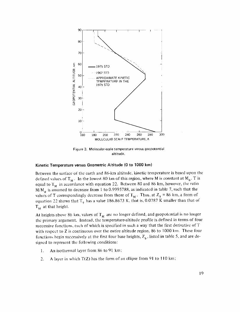
T M of H is completely defined from the surface to 84.852 km' (86 km). A graph of this
function compared to the similar function of the 1962 Standard is shown in figure 3. From
the surface of the earth to the 51-kin' altitude, this profile is identical to that of the 1962
Standard. The profile from 51 to 84.852 km' was selected in accordance with present-day
data, and abbreviated tables of thermodynamic properties of the atmosphere based upon
this temperature-height profile were published by Kantor and Cole (1973).
18
90 __m
8O
7O
6O
u5E3
50
--g 4oI--ZuJt--oo_ 30oUA
2O
10
0160 300
',i ' ' i , rI ,
1975 STD __
- - 1962 STD "_i
...... APPROXIMATE KINETIC ,I
TEMPERATURE IN THE /
I 1 I I I
180 200 220 240 260 280
MOLECULAR-SCALE TEMPERATURE, K
Figure 3. Molecular-scale temperature versus geopotential
altitude.
Kinetic Temperature versus Geometric Altitude (0 to 1000 km)
Between the surface of tile earth and 86-km altitude, kinetic temperature is based upon the
defined values of T M . In the lowest 80 km of this region, where M is constant at M o , T is
equal to T M in accordance with equation 22. Between 80 and 86 kin, however, the ratio
M/M o is assumed to decrease from 1 to 0.9995788, as indicated in table 7, such that the
values of T correspondingly decrease from those of T M. Thus, at Z v = 86 km, a form of
equation 22 shows that Tv has a value 186.8673 K, that is, 0.0787 K smaller than that of
TM at that height.
At heights above 86 km, values of T M are no longer defined, and geopotential is no longer
the primary argument. Instead, the temperature-altitude profile is defined in terms of four
successive functions, each of which is specified in such a way that the first derivative of T
with respect to Z is continuous over the entire altitude region, 86 to 1000 kin. These four
functions begin successively at the first four base heights, Z b , listed in table 5, and are de-
signed to represent the following conditions:
1. An isothermal layer from 86 to 91 kin;
2. A layer in which T(Z) has the form of an ellipse from 91 to 110 km;
19
3. A constant,positive-gradientlayerfrom 110to 120km:and
4. A layerin whichT increasesexponentiallytowardanasymptote,asZ increases
from 120 to 1000 kin.
86 to 91 km
For the layer from Z 7 = 86 km to Z s = 91 km, the temperature-altitude function is defined
to be isothermally linear with respect to geometric altitude, so that the gradient of T with
respect to Z, is zero (see table 5). Thus, the standard form of the linear function, which is
degenerates to
T = Tb +LK, b " (Z- Zb) (24)
T = T 7 = 186.8673 K (25)
and by definition
dT-- = 0.0 K/kin (26)dZ
The value of T 7 is derived from one version of equation 22 in which T M is replaced by
TM, 7 = 186.946 from equation 23 or from table 3, and M/M 0 is replaced by the value
0.9995788 from table 7. Thus, T 7 = 186.8673 K. Since the kinetic temperature, T, is
defined to be constant for the entire layer, Z 7 to Z 8 , the temperature at Z 8 is T 8 = T 7
= 186.8673 K, and the gradient, dT/dZ, at Z 8 is LK,8 = 0.0 K/km, the same as for LK,7 .
91 to 110 km
For the layer Z 8 = 91 km to Z 9 = 110 kin, the temperature-altitude function is defined tobe a segment of an ellipse expressed by
[( )2]12Z- Z8T = Tc+A" 1-
a
(27)
where
T c = 263.1905 K, derived in Appendix B,
A = -76.3232 K, derived in Appendix B,
a = -19.9429 km, derived in Appendix B,
and Z is limited to values from 91 to 110 km.
2O
Equation27 isderivedin AppendixB from thebasicequationfor anellipse,to meetthevaluesof T8andLI<,8derivedabove,aswellasthedefinedvalues T 9 = 240 K and
LK,9 = 12 K/km, for Z 9 = 110 km. With these restraints, the values of T c , a, and A arefound to be those cited above.
The expression for dT/dZ related to equation 27 is
( ( )21,J2• z- z 8dT -A Z- Z8 1dZ a a a
(28)
110 to 120 km
For the layer Z 9 = 110 km to Z_o = 120 km, T(Z) has the form of equation 24, where
subscript b is 9, such that T b and LK,b are, respectively, the defined quantities T 9 and LK,9(see Category I|1 Constants and table 5 respectively), while Z is limited to the range 110 to
120 kin. Thus,
T = T 9 +LK,9(Z- Z 9) (29)
and
dT
dZ LK, 9 12.0 K/kin (30)
Since dT/dZ is constant over the entire layer, LK, IO, the value of dT/dZ at Zlo, is identical
to LK, 9 (that is, 12 K/kin) while the value of Tlo at Zlo is found from equation 29 to be360 K.
120 to 1000 km
For the layer Z_o(Walker, 1965)
such that
= 120 to Z12 = 1000 km T(Z) is defined to have the exponential form
T = T®- (T- TI0)" exp (-X" _) (31)
r + Zl0) 2d__Y.Y=X" (T - TlO) • "exp(-X'_)dZ = r0 + Z
(32)
because _. = LK, 9/(T = - Tl0)= 0.01875,
and = _(Z) = (Z- Zlo) (ro + Zlo)/(r o + Z)
21
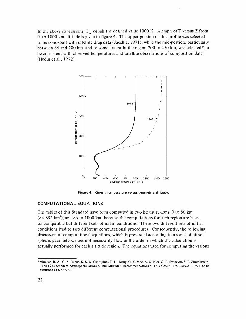
In the above expressions, Too equals the defined value 1000 K. A graph ofT versus Z from
0- to 1000-kin altitude is given in figure 4. The upper portion of this profile was selected
to be consistent with satellite drag data (Jacchia, 1971), while the mid-portion, particularly
between 86 and 200 kin, and to some extent in the region 200 to 450 km, was selected* to
be consistent with observed temperatures and satellite observations of composition data
(Hedin et al., 1972).
500 -- I 7 _
400
300
o
_ 2oo
100
1975 /
I
l
f
f
f
J
l
l
/1962
I
/
/
//
/
iO0 200 400 600 800 1000 1200 1400 1600
KINETIC TEMPERATURE, K
Figure 4. Kinetic temperature versusgeometric altitude.
COMPUTATIONAL EQUATIONS
The tables of this Standard have been computed in two height regions, 0 to 86 km
(84.852 km'), and 86 to 1000 kin, because the computations for each region are based
on compatible but different sets of initial conditions. These two different sets of initial
conditions lead to two different computational procedures. Consequently, the following
discussion of computational equations, which is presented according to a series of atmo-
spheric parameters, does not necessarily flow in the order in which the calculation is
actually performed for each altitude region. The equations used for computing the various
*Minzner, R. A., C. A. Reber, K. S. W. Champion, F. T. Huang, O. K. Moe, A. O. Nier, G. R. Swenson, S. P. Zimmerman,
"The 1975 Standard Atmosphere Above 86-km Altitude: Recommendations of Task Group II to COESA," 1974, to be
published as NASA SP.
22
propertiesof the atmosphere for altitudes below 86 km are, with certain noted exceptions,
equivalent to those used in the 1962 Standard, and the various equations involving T M stem
from expressions used in the ARDC Model Atmosphere, 1956 (Minzner, 1956).
Pressure
Three different equations are used to compute pressure, P, in various height regimes of this
Standard. One of these equations applies to heights above 86 km, while the other two apply
to the height regime from the surface of the earth up to 86-kin altitude, within which re-
gime the argument of the computation is geopotential. Consequently, expressions for com-
puting pressure as a function of geopotential altitude stem from the integration of equation?
5 after replacing g • dZ by its equivalent go dH from equation 16, and after replacing the
ratio M/T by its equivalent Mo/T o in accordance with equation 22. Two forms result from
this integration-one is for the case when LM,b for a particular layer is equal to zero, and the
other when the value of LM,b is not zero. The latter of these two expressions is
?
I 1TM, b R* " LM, b
P = Pb" (33a)TM, b + LM, b • (H - H b)
and the former is
I ]-go " M0(H- Hb)
P = Pb " exp R* " TM,b(33b)
Equation 33a is used for layers associated with values of subscript b equal to 0, 2, 3, 5 and
6; equation 33b is used for layers associated with values of subscript b equal to 1 and 4.
P
In these equations, go' Mo' and R* are each defined single-valued constants, while LM,b and
H b are each defined multi-valued constants in accordance with the value of b as indicated
in table 3. In each equation, H may have values ranging from H b to Hb+1 . The quantity
TM, b is a multi-valued constant listed in table 3 with values derived from equation 23 in
accordance with the several values of b and the corresponding defined values of LM,b and
H b . The reference-level value of Pb for b = 0 is the defined sea-level value, Po = 101.3250
kPa (equivalently 101325 N/m 2 or 1013.25 mbar). The values of P b for b = 1 throughb = 6 are obtained from the application of the appropriate member of the pair of equations
33a and 33b for the case when H = Hb+ l .
These two equations applied successively yield the pressure for any desired geopotentiai
altitude from sea level to HT, where H 7 is the geopotential altitude corresponding to the
geometric altitude Z 7 = 86 kin. Pressures for H from 0 to -5 kin' may also be computedfrom equation 33a when b = 0.
23

For Z equalto 86km andabovethevalueof pressureiscomputedasafunctionof geome-tric altitude,Z, andinvolvesthe altitude profile of kinetic temperature, T, rather than that
of T M, in an expression in which the total pressure, P, is equal to the sum of the partialpressures for the individual species as expressed by equation 3. Thus, for Z = 86 to 1000 km,
Y_ni • R* • TP = _;Pi = Y_ni " k • T = (33c)
Nn
In this expression,
k = the Boltzmann constant, defined in Category I,
T = T(Z) defined in equations 25, 27, 29, and 31 for successive layers,
1= the sum of the number densities of the individual gas species comprising the
atmosphere at altitude Z above 86 kin, as described below.
Neither ni, the number densities of individual species, nor En i, the sum of the individualnumber densities, is known directly. Consequently, pressures above 86 km cannot be com-
puted without first determining n i for each of the significant gas species.
Number Density of Individual Species
In the height region of complete mixing (0 to 80 km), ni, the number density of any parti-
cular major gas species varies with altitude in accordance with the altitude variation of the
total number density, N. For this height region, the value of the ith species is, therefore,
given by
n i = Fi • N (34)
where F. is the constant fractional volume coefficient given for each species in table 2.1
Since the values of N listed in the detailed tables of this Standard are not completely con-
sistent with the basic definition of the model between 80 and 85 km, as previously dis-
cussed, values of n i calculated from tabulated values of N for this limited height regime,
must be corrected by dividing by the appropriate values of M/M 0 from table 7. At altitudes
above 86 km, equation 34 no longer applies, since the model assumes the existence of vari-
ous processes which lead to particular differing height variations in the number-density
values of several individual species, N 2 , O, 02 , Ar, He, and H, each governed by equation 6.
Ideally, the set of equation 6, each member of which is associated with a particular species,
should be solved simultaneously, since the number densities of all the species are coupled
through the expressions for molecular diffusion which are included in equation 6. Such a
solution would require an inordinate amount of computation, however, and a simpler
approach was desired. This was achieved with negligible loss of validity by some simplifying
approximations, and by calculating the number densities of individual species one at a time
in the order n(N 2 ), n(O), n(O 2 ), n(Ar), n(He), and n(H). For all species except hydrogen
(which is discussed later), we divide equation 6 by ni and integrate directly, to obtain the
following set of simultaneous equations, one for each gas species:
24

T7 (v l I.... exp f(Z) + dZni ni. 7 T z7
(35)
In this set of equations,
ni, 7 = the set of species-dependent, number-density values for Z = Z 7 = 86 km,one member for each of the five designated species, as derived in Appen-
dix A and listed here,
N 1.129794 X 10²⁰ m 3
O 8.6 X 10¹⁶ m 3
02 3.030898 X 10¹⁹ m "3Ar 1.351400 X 10¹⁸ m "3
He 7.5817 X 101° m a
T 7
T
f(Z)
vi/(D i + K)
= 186.8673 K, the value of T at Z 7 , as specified in equation 25,
= T(Z) defined by equations 25, 27, 29, and 31 for the appropriate altitude
regions,
= the function written as equation 36 below,
= the set of empirical functions written as equation 37 below
For f(Z) we have
where
d;z1- . • Mi+--+---f(Z) R* • T D i g
(36)
D.I
M.1
l
dT/dZ =
M
Di(Z) as defined by equation 8 for the ith species,
K(Z) as defined by equations 7a, 7b, and 7c,
the molecular weight of the ith species as defined in table 2,
the thermal diffusion coefficient for the ith species as defined in table 4,
one of equations 26, 28, 30, or 32, as appropriate to the altitude region,
= M(Z), with special considerations mentioned below.
For [vi/(Di + K)] we have the following set of empirical expressions.
V i
- Qi " (Z- Ui )2 • exp [-W i ° (Z- Ui )3 ]
+ qi " (Ui- z)2 " exp [-w i • (u i - Z) 3 ]
D.+K1 (37)
25

The set of expressions represented by equation 37, while representing a function of both D i
and K, does not directly involve calculated values of either of these coefficients. Rather, it
involves a series of six other coefficients which, for each of four species, have been empiri-
cally selected to adjust the number-density profile of the related species to particular values
in agreement with observations. The defined values of the six sets of species-dependent
c°efficients-qi, Qi, ui, Ui, wi, and Wi used in equation 37-are listed in table 6. The values
of qi and Ui were selected so that for 02 , Ar, and He, the quantity vi/(D i + K) becomes
zero at exactly 86 kin. For atomic oxygen, however, all six of these coefficients contribute
to maximizing this quantity for Z = 86 kin.
Molecular Nitrogen
Molecular nitrogen (N 2 ) is the first species for which n is calculated. On the average, the
distribution of N 2 is close to that for static equilibrium, and hence, for this species, we
may neglect the transport velocity, thereby eliminating the term [vi/(D i + K)] from that
version of equation 35 applying to N2 . This species is dominant above and below the
turbopause, and its molecular weight is close to the mean molecular weight in the lower
thermosphere, where mixing still dominates the distribution process. The effect of mixing
up to 100-km altitude is approximated therefore by two additional adjustments to equation
35 as applied to N 2 . Both adjustments are implicit in f(Z); these are neglecting K and re-
placing Mi by the mean molecular weight M which, for the altitude region 86 to 100 km,,,
is approximated by M0. With these three adjustments, that version of equation 35 applying
to N 2 reduces to
, 1n(N 2) = n(N2) 7 "--_--'exp R* • Tz 7
where
M = M0 for Z _< 100 km, and
M = M(N 2)forz>100km.
Figure 5 shows a graph of n(N 2 ) versus Z.
Species O, 02 , Ar, and He
As noted above, after the calculation of n(N 2) has been performed, the values of n i for the
next four species are calculated from equation 35 in the order O, 02 , Ar, and He. In the
case of O and 02 , the problem of mutual diffusion is simplified by considering N 2 as thestationary background gas (as described in the previous section). For Ar and He, which
are minor constituents in the lower thermosphere, it is more realistic to use the sum of
the number densites of N 2 , O, and 02 as the background gas in evaluating the molecular-
diffusion coefficient, Di, and the mean-molecular weight, M, except below 100 km where
26

900
8OO
i00
0
108 i01o
Olm
02------
N 2 ....
Ar .......
H 1 ....
He .......
TOTAL -----
1026
Figure 5. Number density of individual speciesand totalnumber density versusgeometric altitude.
M is taken to be the sea-level value, Mo . This latter choice is to maintain consistency with
the method for calculating n(N 2 ).
In equation 37, defining [vi/(O i + K)], the coefficients qi, Qi' ui' Ui' wi' and Wi, which
(except for qi ) are constant for a particular species, are each adjusted such that appropriate
densities are obtained at 450 km for O and He, and at 150 km for O, 02, He, and Ar. The
constant qi' and hence the second term of equation 37, is zero for all species except atomicoxygen, and is also zero for atomic oxygen above 97 km; the extra term for atomic oxygen
is needed below 97 km to generate a maximum in the density-height profile at the selected
height of 97 km. This maximum results from the increased loss of atomic oxygen by re-
combination at lower altitudes. The flux terms for O and 02 are based on, and lead (quali-
tatively) to the same results as those derived from the much more detailed calculations by
Colegrove et al. (1965) and Keneshea and Zimmerman (1970) and discussed in Appendix
D.
A further computational simplification is realized above 115 km where the eddy-diffusion
coefficient becomes zero. For these altitudes, the set of expressions represented by equa-
tion 35 becomes uncoupled, and each member reduces to a form where the integration is
performed only on the sum of three terms:
1. The barometric term for the particular species (that is, the right-hand side of
equation 5),
27
2. Thethermal-diffusionterm (o_i/T) • (dT/dZ),
3. A simplified velocity term.
In the case of O, 02 , and Ar, the thermal-diffusion term is zero. Also, as may be shown,
the velocity term, [vi/(D i + K)], becomes small above 120 km and, with the exception ofatomic hydrogen, each species considered is nearly in diffusive equilibrium at these heights.
For the present model, however, this situation becomes exactly true only at altitudes above
150 km.
The altitude profile of number density for each of the species O, 02 , Ar, and He is given
in figure 5, along with that for N 2 .
Atomic Hydrogen
For various reasons, the height distribution of the number density of atomic hydrogen,
n(H), is defined only for heights from 150 to 1000 km. Below 150 km, the concentration
of H is negligible compared with the concentrations of O, 02, Ar, and He. The defining
expression for n(H), like the expression for n(N 2 ), n(O), and so on, is derived from equa-tion 6. The solution for n(H), however, is expressed in terms of the vertical flux, n(H)
• v(H) represented by q_,rather than in terms of v(H), because it is the flux which is con-
sidered known for H. In this model, only that contribution to _bdue to planetary escape
from the exosphere is considered.
Since K is zero for the altitude region of interest, the particular version of equation 6 ap-
plied to H is correspondingly simplified, and one possible solution to the resulting expres-
sion is
where
n(H)11
D(H)
T
Tll
n(H) = n(H)ll- D(H)11
__) l+atH) (exp r)
•(expr)'dZ]
(39)
= 8.0 × 10 l° m 3, the number density of H at Zll = 500 km, as defined in
Category III Constants,
= the molecular diffusion coefficient for hydrogen given by equation 8 in which
the values of a i and b i are as defined in table 4,
= 7.2 X l0 II m-2 • s1 , the vertical flux of H, as defined in Category III Constants,
= T(Z) as specified by equation 31,
= 999.2356 K, the temperature derived from equation 31 for Z = Zll,
28

_(H)
T
= the thermal diffusion coefficient for H, -0.25 (dimensionless), as defined in
table 4,
= r(Z) defined in equation 40
fzl z g- M(tt) dZ (40)r= R*'Tl
Because D(H) becomes very large compared with _ for heights above 500 km, the value of
the integral term in equation 39 can be neglected at these heights, and atomic hydrogen is
then essentially in diffusive equilibrium. Figure 5 depicts the graph of n(H) as a function
of Z, along with those of other species.
Mean Molecular Weight (Above 86 km)
Equations 35 through 39 permit the calculation of the number densities of the species N 2 ,
O, 02 , Ar, He, and H for heights above 150 km, and of the first five of these species forheights between 86 and 150 km, where n(H) is insignificant compared with n(N 2 ). These
number densities permit the calculation of several atmospheric parameters in the height
region 86 to 1000 km. The first is mean molecular weight using equation 20. These values
of M, along with those implicit in table 7 for Z from 80 to 86 km, plus the invariant value,
M0, for heights from 0 to 80 kin, are shown in figure 6.
900
8°°I700
E_: 600
500
(.3
400taJ
I
S300
200
1O0 _r
I
Figure6.
h ' _46 10 18 22 26 30
MOLECULAR WEIGHT, kg/kmol
Mean molecular weight versusgeometric altitude.
29

Pressure and Mass Density (Above 86 km)
The number densities of the several species also permit us now to compute total pressure
and mass density for heights from 86 to 1000 kin, using equation 33c, and one version of
equation 1. Figure 7 depicts these values as well as those for heights below 86 km computed
from equations 33a and 33b. Finally, these individual number densities permit the calcula-
tion of total number density, N = Zn i, at heights from 86 to 1000 km.
looO
9oo
8OO
2oo
100
DENSITY, kg/m 3
10 -14 10 -12 10-10 10 -8 10-6 10 -4 10-2 10 0
\
10 -8 10-6 10-4 10-2 10 0 10 2 10 4 10 6
PRESSURE, N/m 2
Figure 7. Total pressure and mass density versus
geometric altitude.
Total Number Density
From equations 2, 22, and 33c, it is apparent that total number density, N, the number of
neutral gas particles per unit volume of the atmosphere, may be expressed in any one of
the following three equivalent forms:
M0 • N A • p NA • pN - - - Xn i (41)
TM ' R* • M R* • T
30
The three forms are selected to satisfy three types of calculations:
1. Those depending upon values of T M ,
2. Those depending upon values of T, and#
3. Those depending upon values of ]_n i.
This format will be followed in specifying the computational equations, insofar as possible,
for the balance of the quantities discussed in this document. A graph of the altitude varia-
tion of total number density is presented in figure 5, along with the number densities of
individual species. That portion of equation 41 involving T M is of particular interest in
calculating N for heights from 0 to 86 km.
Mass Density
From equations l, 22, and 33c, one may write the following three forms of computational
equations for mass density, p:
P " M0 P" M Z(n i" Mi)0 .... (42)
R* " T M R* • T N A
The altitude-dependent variations of this quantity are shown in figure 7 along with those
of pressure.
Mole Volume
Mole volume, Vm, of air is defined as the volume of one mole of air, where one mole of air
is the amount consisting of a number of neutral particles equal to N A . In S.I. units, the
quantity vm should specify the number of cubic meters containing 1 kmol of air. Since Mhas the dimensions of kg/kmol, and p has the dimensions of kg/m 3 , the ratio M/O, with the
units m 3/kmol, provides the definition of mole volume. Ill terms of equations 1, 22, and
33c, this ratio may be equated to the following series of expressions:
vm
R*" M "T M R*" T NA
M0 • p P _n i(43)
This quantity, while not tabulated in this Standard, is shown graphically in figure 8.
Scale Height
Pressure Scale Height
The quantity R* • T/(g • M), which has dimensions of length, is commonly associated with
the concept of scale height and is the defining form of pressure scale height, Hp, used in
this model. Thus, equations 20 and 22 may be written:
31
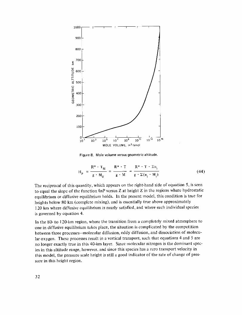
1000 I i I I l
900
800
700E
600
500
w 400
o
3OO
200
100
0 I i I I10 1 103 105 107 109 1011 1013
MOLE VOLUME, m3/kmol
1015
Figure 8. Mole volume versus geometric altitude.
R* • TM R* • T R* • T • Zn iHp - - (44)
g. M 0 g" M g'_(n i • Mi)
The reciprocal of this quantity, which appears on the right-hand side of equation 5, is seen
to equal the slope of the function £nP versus Z at height Z in the regions where hydrostatic
equilibrium or diffusive equilibrium holds. In the present model, this condition is true for
heights below 80 km (complete mixing), and is essentially true above approximately
120 km where diffusive equilibrium is nearly satisfied, and where each individual species
is governed by equation 4.
In the 80- to 120-km region, where the transition from a completely mixed atmosphere to
one in diffusive equilibrium takes place, the situation is complicated by the competition
between three processes-molecular diffusion, eddy diffusion, and dissociation of molecu-
lar oxygen. These processes result in a vertical transport, such that equations 4 and 5 are
no longer exactly true in this 40-kin layer. Since molecular nitrogen is the dominant spec-
ies in this altitude range, however, and since this species has a zero transport velocity in
this model, the pressure scale height is still a good indicator of the rate of change of pres-
sure in this height region.
32
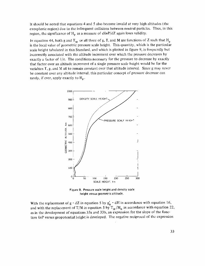
It shouldbenotedthat equations4 and5alsobecomeinvalidat veryhighaltitudes(theexosphericregion)dueto theinfrequentcollisionsbetweenneutralparticles.Thus,in thisregion,thesignificanceof HFasameasureof d£nP/dZagainlosesvalidity.
In equation44,bothgandTM or all threeof g,T,andM arefunctionsof Z suchthat Hpis the localvalueof geometricpressurescaleheight. Thisquantity,whichis theparticularscaleheighttabulatedin this Standard,andwhichisplottedin figure9,is frequentlybutincorrectlyassociatedwith thealtitudeincrementoverwhichthepressuredecreasesbyexactlyafactorof 1/e. Theconditionsnecessaryfor thepressureto decreaseby exactlythat factoroveranaltitudeincrementof a singlepressurescaleheightwouldbefor thevariablesT, g,andM all to remainconstantoverthat altitudeinterval. Sincegmayneverbeconstantoveranyaltitudeinterval,thisparticularconceptof pressuredecreasecanrarely,if ever,applyexactlyto Hp.
E
u_c3
O
OLLlo
,°°°/
800
70O
600
5O0
400
300
20O
i i
DENSITY SCALE
100
i i 1 L
O0 50 i00 150 200 250 300
SCALE HEIGHT, km
Figure 9. Pressurescaleheight and density scaleheight versusgeometric altitude.
With the replacement of g • dZ in equation 5 by go " dH in accordance with equation 16,
and with the replacement of T/M in equation 5 by T M/M o in accordance with equation 22,
as in the development of equations 33a and 33b, an expression for the slope of the func-
tion £nP versus geopotential height is developed. The negative reciprocal of the expression
33

t
for this slope is called geopotential pressure scale height, Hp, and it has the same dimensions
as geopotential height. Tile quantity He is implicit in the computational pressure equations
33a and 33b. This concept of scale height may be expressed as follows:
, = __(-d_nP/-1 R*- T M R*" T (45)Hp i t -- i
\ dH l go " M0 go " M
Within a layer of constant T u , or of constant ratio T/M, the pressure does, in fact, decrease
by exactly 1/e of its initial value when the geopotential altitude increases by exactly one
geopotential scale height. This is precisely the situation expressed by equation 33b which,?
in terms of H e , may be rewritten as
P = Pb'exp --H_ (46)
Equation 45 is rigorously valid only below 80 kin, while equation 46 applies only within
isothermal layers below 80 km.
Density Scale Height
Because of the relationship between Hp and the slope of _nP versus Z it is convenient to
apply the name geometric density scale height, H ° , to the negative reciprocal of the slopeof _np versus Z. Using the equation of state (equation 1) to relate d£np to d_nP, one may
Hp Hp
define
HP = (d_dnTM/_ I + Hp" (d_nT d£nM) (47)1 + Hp • \ dZ ] \ dZ dZ
The relationships implied between H ° and d_np/dZ are subject to the same limitations as
those between H e and d£nP/dZ expressed above, that is, Hp is only an approximation to(d_np/dZ) -1 between 80 and 120 km and in the exosphere, where the approximation be-
comes increasingly invalid with increasing altitude.
Within these limitations, it is apparent that in layers where T M does not change with
changing altitude, that is, where (d_nT M/dZ) = 0, H o is equal to Hp. Within such layers,the slope of £nP versus Z at any particular altitude Z is identical to the slope of £nP versus
Z, but neither P nor p decreases by a factor of 1/e when altitude increases by an amount
He = H ° .
While density scale height is not tabulated in this Standard, values of this quantity are
shown graphically with those of H e in figure 9.
34

If, however,ageopotentialdensityscaleheight,H'p, isdefinedasthenegativereciprocaloftheslopeof £npwith respectto geopotential,onemaywrite
t P
l+H;-i-7--,f \7, !I
This quantity is equal to He in a layer within which T M is constant, and for this condition,
H t specifies the altitude change for which p changes by a factor of 1/e. The quantity H'p P
permits the writing of a density-altitude equation analagous to the pressure-altitude equa-
tion, equation 33b, but in terms of H' "P
H- Hb)P = Pb " exp -H_ (49)
As in the case of equation 45, equation 49 is rigorously valid only below 80 km, while
equation 49 applies only within isothermal layers below 80 km.
Mean Air-particle Speed
The mean air-particle speed, V, is the arithmetic average of the speeds of all air particles in
the volume element being considered. All particles are considered to be neutral. For a
valid average to occur, there must be a sufficient number of particles involved to represent
mean conditions. Pressure and temperature gradients within the volume must also be neg-
ligible. The analytical expression for V is closely related to that for the speed of sound,
and is proportional to the ratio T/M. Thus, in terms of equations 20 and 22,
1/2
V = = (50)[8 , = 8" R* • T • 2nil 1/2
- i
rr 7" _(ni Mi )
The variation of particle speed with geometric altitude is shown in figure 10.
Mean Free Path
The mean free path, L, is the mean value of the distances traveled by each of the neutral
particles, in a selected volume, between successive collisions with other particles in that
volume. As in the case of V, a meaningful average requires that the selected volume be
big enough to contain a large number of particles. The computational form for L is
L =
2 1/2 . R* • M • T M 2 1/2 • R* • T 2 1/2= (51)
2)7 • N A • 0 2 • M0 • P 2_ • N A • 0 2 P 2rr" 0 2 • gn i
35
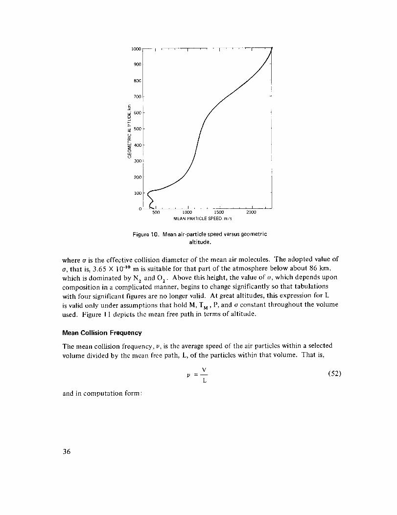
1000 i T I
I
8OO
700 i
600
._ 5oo
w 400
.,o,
3OO _
2OO
5OO
, L , , I L_______10OO ] 500 2000
MEAN PARTICLE SPEED, m/s
Figure 10. Mean air-particle speed versus geometricaltitude.
where o is the effective collision diameter of the mean air molecules. The adopted value of
o, that is, 3.65 × 10⁻¹° m is suitable for that part of the atmosphere below about 86 km,
which is dominated by N 2 and 02 . Above this height, the value of o, which depends upon
composition in a complicated manner, begins to change significantly so that tabulations
with four significant figures are no longer valid. At great altitudes, this expression for L
is valid only under assumptions that hold M, T M , P, and o constant throughout the volume
used. Figure 11 depicts the mean free path in terms of altitude.
Mean Collision Frequency
The mean collision frequency, u, is the average speed of the air particles within a selected
volume divided by the mean free path, L, of the particles within that volume. That is,
V/) =m
L(52)
and in computation form:
36
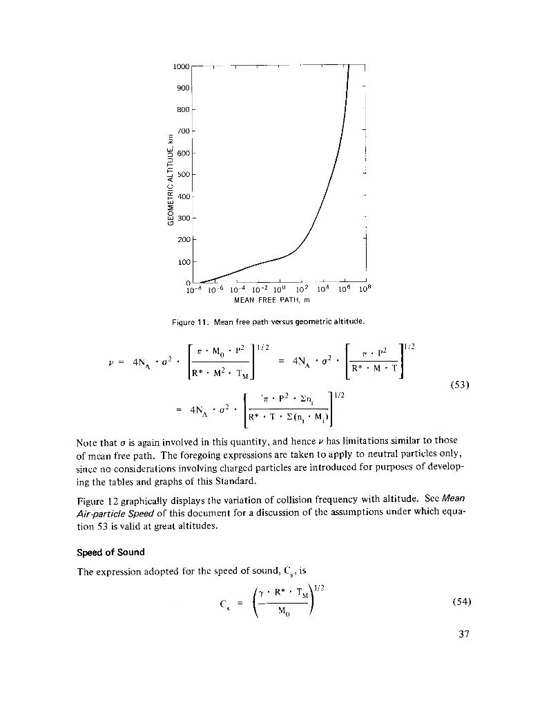
9OO
8OO
700
_600
5ooo
400
0300
200
100
0 I L I l l I
10-8 10-6 10-4 10-2 10 0 10 2 10 4 10 6
MEAN FREE PATH, m
108
Figure 11. Mean free path versus geometric altitude.
u = 4N A • 02 • = 4N A " 02 "R*'M'T
• M 2 T M
(53)
= 4N_. -0 2 " [ 'rr" p2 . I;ni 1|/2
• JR* • T • Z(n i • Mi) 1
Note that o is again involved in this quantity, and hence u has limitations similar to those
of mean free path. The foregoing expressions are taken to apply to neutral particles only,
since no considerations involving charged particles are introduced for purposes of develop-
ing the tables and graphs of this Standard.
Figure 12 graphically displays the variation of collision frequency with altitude. See Mean
Air-particle Speed of this document for a discussion of the assumptions under which equa-
tion 53 is valid at great altitudes.
Speed of Sound
The expression adopted for the speed of sound, Cs, is
7 ° R* " T M
c= Mo(54)
37
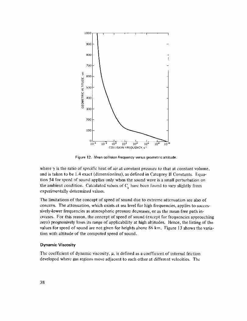
900
800
700
E600
500
_ 4oo
3OO
200
10o
olO-4 10-2 10 0 10 2 lO 4 10 6 lO 8 lO 1°
COLLISION FREQUENCY, s-'
Figure 12. Mean collision frequency versus geometric altitude.
where 7 is the ratio of specific heat of air at constant pressure to that at constant volume,
and is taken to be 1.4 exact (dimensionless), as defined in Category II Constants. Equa-
tion 54 for speed of sound applies only when the sound wave is a small perturbation on
the ambient condition. Calculated values of Cs have been found to vary slightly fromexperimentally determined values.
The limitations of the concept of speed of sound due to extreme attenuation are also of
concern. The attenuation, which exists at sea level for high frequencies, applies to succes-
sively-lower frequencies as atmospheric pressure decreases, or as the mean free path in-
creases. For this reason, the concept of speed of sound (except for frequencies approaching
zero) progressively loses its range of applicability at high altitudes. Hence, the listing of the
values for speed of sound _are not given for heights above 86 kin. Figure 13 shows the varia-
tion with altitude of the computed speed of sound.
Dynamic Viscosity
The coefficient of dynamic viscosity, p, is defined as a coefficient of internal friction
developed where gas regions move adjacent to each other at different velocities. The
38
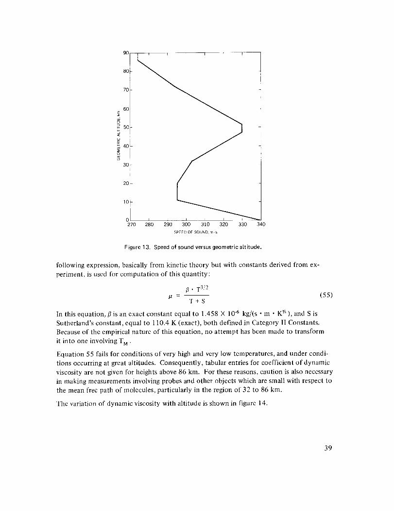
90 I i P I I I ]
80
7O
6O
u5£5
_-D50[-
i_0 ,ec I
_ 40L
ow
o 30 t
20
10
o270 280 290 300 31o 320 330 340
SPEED OF SOUND, m/s
Figure 13. Speed of sound versus geometric altitude.
following expression, basically from kinetic theory but with constants derived from ex-
periment, is used for computation of this quantity:
ft. T3/2
U - (55)T+S
In this equation,/3 is an exact constant equal to 1.458 × 10 -6 kg/(s • m • Ky2), and S is
Sutherland's constant, equal to 110.4 K (exact), both defined in Category II Constants.
Because of the empirical nature of this equation, no attempt has been made to transform
it into one involving T M .
Equation 55 fails for conditions of very high and very low temperatures, and under condi-
tions occurring at great altitudes. Consequently, tabular entries for coefficient of dynamic
viscosity are not given for heights above 86 km. For these reasons, caution is also necessary
in making measurements involving probes and other objects which are small with respect to
the mean free path of molecules, particularly in the region of 32 to 86 km.
The variation of dynamic viscosity with altitude is shown in figure 14.
39
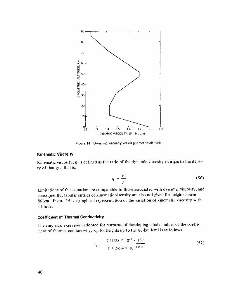
iI 1 I i T I I
8O
7O
6O
£3
t--
_ 5o
(D
_-40
o
N ao
2O
10
01,2 1.L3 114 ll.5 1.6 1.7 1.8 1.9
DYNAMIC VISCOSITY, 10 -5 N . s/m _
Figure 14. Dynamic viscosity versus geometric altitude.
Kinematic Viscosity
Kinematic viscosity, 7, is defined as the ratio of the dynamic viscosity of a gas to the densi-
ty of that gas, that is,
#77 - (56)
P
Limitations of this equation are comparable to those associated with dynamic viscosity, and
consequently, tabular entries of kinematic viscosity are also not given for heights above
86 km. Figure 15 is a graphical representation of the variation of kinematic viscosity with
altitude.
Coefficient of Thermal Conductivity
The empirical expression adopted for purposes of developing tabular values of the coeffi-
cient of thermal conductivity, k t , for heights up to the 86-km level is as follows:
k t
2.64638 X 10 3 • T 3/2
T + 245.4 X 10(12/T)(57)
40

8O
7O
6O
5O
4O
3O
2O
i0
010 -5 10 4 10 -3 10 -2 10 -1 10 0 lO t
KINEMATIC VISCOSITY, m2/s
Figure 15. Kinematic viscosity versusgeometric altitude.
This expression differs from that used in the U.S. Standard Atmosphere, 1962 (COESA,
1962), in that the numerical constant has been adjusted to accommodate a conversion of
the related energy unit from the temperature-dependent kilogram calorie to the invariant
joule. Thus, the values of k t in units of J/(s • m • K) or W/(m • K) are greater than the
values of kt in units ofkcal/(s • m • K) by a factor of exactly 4.1858 × 10³ , when thekilocalorie is assumed to be the one for 15°C. Kinetic-theory determinations of thermal
conductivity of some monatomic gases agree well with observation. For these gases, ther-
mal conductivity is directly proportional to the dynamic viscosity. Modification of the
simple theory has accounted in part for differences introduced by polyatomic molecules
and by mixtures of gases. Tabular entry of values for coefficient of thermal conductivity
is terminated at 86 kin. The variation with height of this quantity is shown in figure 16.
41
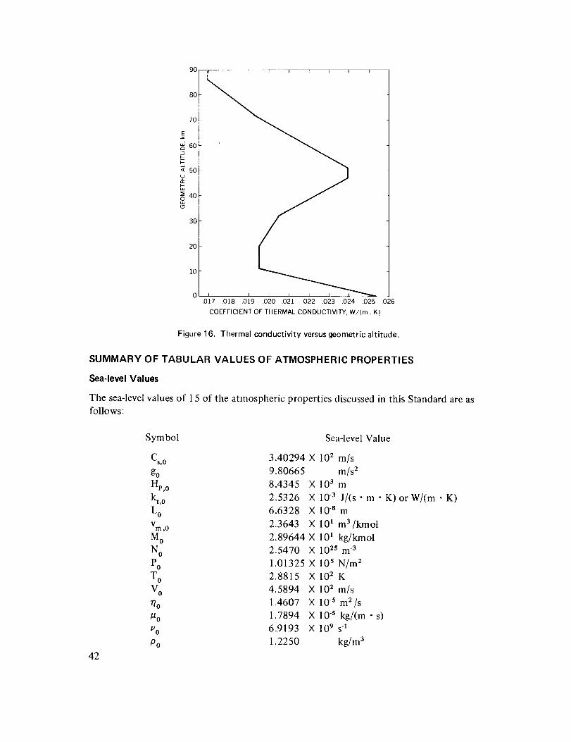
7O
3O
20I10
0 L i _ _ _ l l i
.017 .018 .019 .020 .021 .022 .023 .024 025 .026
COEFFICIENT OF THERMAL CONDUCTIVITY, W/(m. K)
Figure 16. Thermal conductivity versusgeometric altitude.
SUMMARY OF TABULAR VALUES OF ATMOSPHERIC PROPERTIES
Sea-level Values
The sea-level values of 15 of the atmospheric properties discussed in this Standard are asfollows:
42
Symbol Sea-level Value
C,, o 3.40294 X
go 9.80665
Hl,,o 8.4345 X
kt, o 2.5326 X
L o 6.6328 Xv 2.3643 ×
m ,0
Mo 2.89644 X 101 kg/kmol
N o 2.5470 X 10²s m 3
Po 1.01325 X l0 s N/m 2
T O 2.8815 X 10² K
V o 4.5894 X 10² m/s
r/o 1.4607 X 10 s m2/s
_o 1.7894 X 10 s kg/(m's)
vo 6.9193 X 10 9 S"1
Po 1.2250 kg/m 3
102 m/s
m/s 2
103 m
10 -3 J/(s " m • K)or W/(m • K)10-8 m
101 m3/kmol

Thesea-levelvaluesfor g,P,andT aredefinedquantities;theremainderarequantitiescal-culatedfrom theprecedingequations.
Conversion of Metric to English Units
For those who have need to work in the English System of Units, the conversion factors
listed in table 8 are applicable to the atmospheric parameters tabulated or shown graphi-
cally in this Standard. For other transformations, see Mechtly (1973).
Table 8
Metric to English Conversion Factors for Properties of the
U.S. Standard Atmosphere, 19 75 (COESA, 1975)
Symbol
s
g
Hp
k tL
V m
M
N
P
T or T MV
r/
,u.u
P
To Convert from
Metric Units
m/sm/s 2
m
W/(m • K)
m
m 3/kmol
To English
Units
ft/s 3.048
ft/s 2 3.048
Divide by
ft 3.048 × 10 "1*
BTU/(ft • s • °R) 6.226 477 504 X 10 .3
ft 3.048 × 10 -1 *
ft3/lbmol 6.242 796 057 × 10 .2
kg/kmolm-3
mbar
K
m/s
m 2/s
N • s/m 2
S-1
kg/m 3
lb/lbmol
ft-3
in Hg (32°F)
o R
ft/s
ft2/s
lb/(ft • s)
S-1
lb/ft 3
1.000"
3.531 466 672 X 102
3.386 389 X l01
5/9*
3.048 X 10 "1 *
9.290 304 X 10 -2.
1.488 163 944
1.000
1.601 846 3 X 101
*Exact definition.
Tables of Atmospheric Properties
Detailed tables of the height-dependent values of the various atmospheric properties de-
fined by this standard have been prepared elsewhere (COESA, 1975). Abbreviated versions
of these tables are presented at the end of this section in tables 9 through 15. The first four
of these tables, 9 through 12, list atmospheric properties as a function of the boundary
heights of the seven layers adopted to define the temperature-height profile between the
surface of the earth and 86-kin altitude. These boundary heights are specified in integer
multiples of one geopotential kilometer, although the equivalent values of geometric height
are also given.
43

Tables13,14,and 15list theatmosphericpropertiesof thisStandardfor 14selectedalti-tudesin the 86-to 1000-kininterval. Thesealtitudesincludethe boundaryheightsof thefour layersadoptedto definethetemperature-heightprofile in thisheightregion.Becauseof thelargeinterval,120toil000 km,comprisingthehighestlayerof this model,thevaluesof thevariousatmosphericpropertiesin tables13,14,and 15havebeengivenfor nineaddi-tionalheightswithin this layer.
Only threetables(13, 14,and 15)areusedto list thepropertiesof this Standardfor heightsfrom 86 to 1000kin, ascomparedwith four tablesfor theheightregion0 to 86 km. Thisisdueto thefact that, in thisStandard,noneof the fourquantities-speedof sound,dyna-micviscosity,kinematicviscosity,andthermalconductivity-isdefinedfor heightsabove86km. Consequently,table 12,whichliststhevaluesof thesepropertiesbelow86km,hasnocounterpartfor heightsabove86km. Table11,listingnumberdensitiesof fiveatmosphericgasspeciesfor heightsfrom 0 to 86km,hasnocounterpartin thedetailedtablesof theCOESAdocument(COESA,1975).
ACKNOWLEDGMENTS
The authors of this report wish to acknowledge the help and inspiration provided by all the
members of the Working Group of COESA.
Goddard Space Flight Center
National Aeronautics and Space Administration
Greenbelt, Maryland January 2, 1976
Table 9
Temperature, Pressure, and Density versus Geopotential Altitude, 0 to 86 km
Alutude 1
H
km _
0.0000
11.0000
20,0000
32.0000
47,0000
5 ! .0003
71.0000
84.8520
Temperature
• I T
km _ K
q
0.0000 [ 288.150
11.0190 [ 216.650
20.0631 [ 216.650 ~56.500
32.1619 I 228.650 -44.500
47.3500 ] 270.650 - 2.500
51.4124 [ 270.650 - 2500
71.8019 [ 214.650 -58.500
86.0000 t 186,867 I -86.283
Pressure
t T M P P
°C K mbar tort
15.000 288150 1013250+3 760000+2
- 56500 216.650 2,263206 +2 1.69754 +2
216,650 5474889 +1 410650 ÷1
228.650 8.680187 +0 6.51068 +0
270650 1.109063 +0 8.31866-1
270650 6.693887 -1 !5.02083 -1
214,650 3,956420-2 1296756-2
186,946 3733836-3 [2,80061 -3
L
P/Po
1.00000 +0
223361-I1
5.40330-2 1
8,56667-3
1,09456-3
6.60635 -4
3,90468-5
3.68501-6
l_fisity
p [ DIP 0
kCm3 [
I _224999 +0 ! 1.13000 +0
3.639178 -1 2.9708-1
8.803480 - 2 7.1865 - 2
1.322500-2 1.0796-2
1.427532 -3 1.1653-3
8616(149 -4 7.0335 -4
6421099 -5 5.2417 -5
6957879 -6 5.6799 -6
44

Table10SevenSecondaryAtmosphericPropertiesversusGeopotentialAltitude,0 to 86km
Altitude
H I Z g
kin' ] km m,(s 2
0.0000
1 1.0000
20.0000
32.0000
47.0000
51,0000
71,0000
84.8520
0.0000 9.80665
11,0190 9.77274
20,0631 9 74504
32,1619 970817
47,3500 9,66217
51.4124 9.64992
71,8019 9,58881
86,0000 9,54659
Acceleration Pressure
Due to Sc_e
Gra_lty Height
ttp
km
8.4345
6.3636
6.3817
6.7608
8.0407
8.0509
6.4258
5.6212
Number
Density
N
m-3
2.5471 +25
7.5669 +24
1.8305 +24
27499 +23
2.9683 +22
17915 +22
13351 +21
1.4473 +20
Mean
Particle
Speed
V
m/s
458.94
397.95
39795
408 82
444,79
444,79
396,11
396.67
MeanMean Free
CollisionPath
Frequency
v L
sq m
69193 +9 66328-8
17824 +9 22327 -7
43117 +8 9.2295 7
66542 +7 61438 -6
7,8146+6 5.6918 5
] 47166 +6 9.4303 -5
31303 +5 1.2654-3
3,1667 +4 11674 -2
Mean I
Molecular [
Weight [
m h
kg/kmol [
28,9044 I
28.9644
28 9644
28.9644
28,9644
28,9644
28,9644
28.9522
Table 11
Number Densities of Five Species versus Geopotential Altitude, 0 to 86 km
Altitude
H Z n(N/)
km t kill rl1-3
0,0000
11.0000
20.0000
32.0000
47.0000
51.0000
71.0000
84.8520
0,00(30
110190
20.0631
32.1619
47.3500
51,4124
71,8019
86.0000
19888 +25
5,9082 +24
1.4292 +24
2.1471 +23
2.3176 +22
1.3988 +22
1.0425 +21
1.1298 ÷20
.(O)
m-3
8,6 +16
Number Densities
u(O 2) n(A) n(He)
11'1.3 111-3 m'3
5.3353 +24
15850 +24
3.8342 +23
5.7599 +22
6.2174 +21
3.7526 +2l
2.7966 +20
3,0309÷19
2,3789 +23
7,0671 +22
1.7096 +22
2.5682 +21
2.7722 ÷20
1.6732 +20
1.2469 ÷19
135140+18
1.3346 +20
3.9648 ÷19
9,5912 +18
1,4408 *18
1.5553 +17
9.3870 +16
6.9957 +15
75817 +14
45
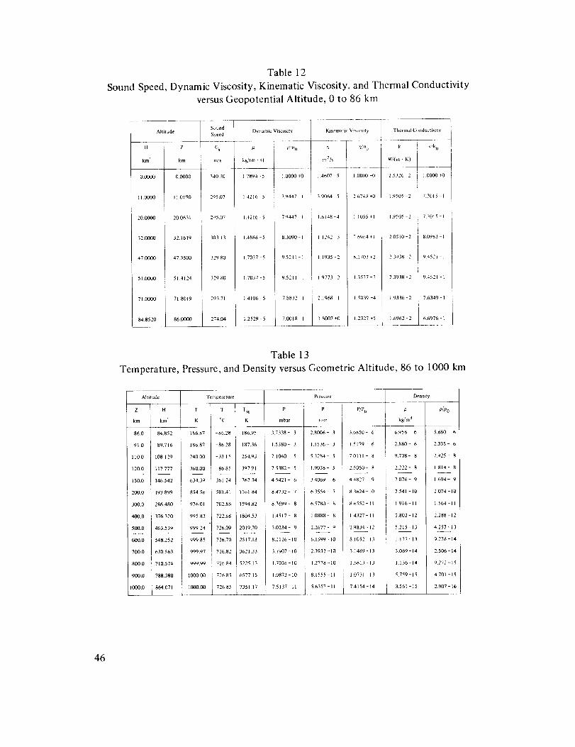
Table12SoundSpeed,DynamicViscosity,KinematicViscosity,andThermalConductivity
versusGeopotentialAltitude,0 to 86km
oundAltitude
peed
It C% _z
low km m,_s kg/Im " s}
I ----+-----_
000 O [ 0.0000 40.30 17894 -5
i
I
11 00, KI ] 11.0190 :)5,07 14216 5
20.00 _0 I 20.0631 0507 14216-5
32.00)0 I 32.1619 0313 1,4868 5
4700)0 t 47 3500 29.80 1.7037 5
I
[ 51 00 )(3 [ 51,4124 29.80 13037 - 5
i
[ 71,00)0 [ 718019 93.71 1.4106 5
I 84.85:0 I 86.0ooo 74,04 1.2529-5
Dynamic Viscosity
O)'!J0 77
m2/s
1.0000 +( 1,4607 - 5
7.9447 I 3.9064 5
79447 I 1.6148 4
83090 I 11242 3
95211 1 1,1935 2
95211 l 19773 2
78832- t 2,1968 I
7.0018 I 18007 ÷0
Kanematic Viscosity
r?,'710
I 0000 +0
2 6743 +0
11055 +1
7 6964 ÷ 1
8.1703 +2
1.3537 +3
1.5039 +4
12327 +5
_'e'(m • K)
25326 2 1.0OO0 +0
1.9505 2 7.7015-1
19505-2 %7015-1
2 05 t0 - 2 8.0983 I
2 3938 "-2 94521 -I
2.3938 2 9.4521-1
t.9336-2 7.6349 1
1.6962 - 2 6.6976 - 1
Table 13
Temperature, Pressure, and Density versus Geometric Altitude, 86 to 1000 km
Altilude Temperature
! T !Z H T
km
86,0
91,0
110,0
120.0
I
150.0
200.0
300.0
400.0
500.0
600.0
700.0
800.0
900.0
000.0
km' K _C
84.852 186.87 -86.28
89.716 186,87 -86.28
108129 240.00 -33.15
117,777 360,00 86.85
146542 63439 361.24
193899 854,56 58141
286.480 976,01 702.86
376.320 995.83 722.68
463.539 99924 726.09I I --
548.252 999.85 726.70
630.563 999.97 726.82
710.574 999.99 726,84
788.380 1000.00 726.85
864.071 1000.00 726.85
I
T M P
K mbar
186,95 3.7338- 3
187,36 15380- 3
254.03 7.1040 5
397,91 2.5382- 5
76234 45421- 6
1161,84 8.4732 - 7
1594.82 8 7699 - 8
1804.53 14517- 8
2019,70 30234- 0
2517.13 8.2126 - 10
3621 33 3.I907 - 10
5225 13 1.7036 - 10
657715 1.0873 -10
7351 17 7.5137 -11
i
Pressure
P
tort
28006- 3
1536- 3
:.3284- 5
.9038- 5I
4069- 6
_3554- 7
,,.5780- 8
.0888- 8
.2677- 9
6,1599 -10
23932 -I0
,2778-10
1,1555-11
L6357-II
Density
P/P0 .o
kghn 3
36850- 6 6.958- 6
15179- 6 2.860- 6
70111- 8 %708- 8
2 5050- 8 2.222- 8
44827- 9 2.076- 9
83624 - 10 2.541 - 10
86552-11 I 916-11
14327 - l t 2£02 - 12
29834-12 5215-13
81052 - 13 1137-13
3 1489 - 13 3.069 - 14
16813 --13 1.136 - 14
10731 13 5.759-15
74154 - 14 3,561 - 15
P/Po
5680- 6
2.335- 6 1
7925- 8
1.814 - 8
1,694- 9
2.074 -I0
1.564-11
2.288 -12
4.257-13
9.278-14
2506 -14
%272 -15
4701-15
2.907-16
46
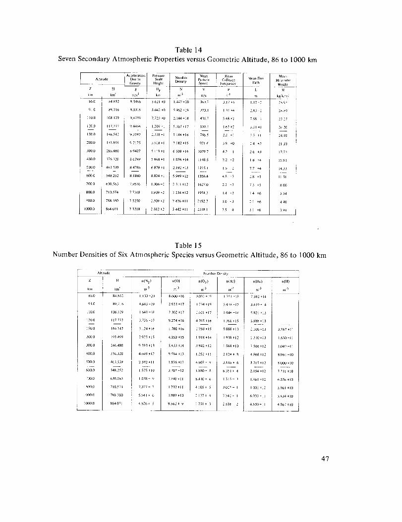
Table14SevenSecondaryAtmosphericPropertiesversusGeometricAltitude, 86to 1000km
ARit ude
Z It
km kin'
86.0 84.852
91.0 89.716
1100 108.129
120.0 117777
1500 146.542
2000 193.899
300,0 286.480
400.0 376320
500.0 463.539
600.0 548252
7000 630563
800.0 710.574
9000 788.380
10000 864.071
Acceleration
Due to
Gravity
g
m/s 2
95466
9.5318
9.4759
9.4466
9.3597
92175
8.9427
86799
8.4286
8.1880
7.9576
77368
7.5250
73218
Pressure
Scale
Height
tip
km
5.621 +0
5,642+0
7723+0
1.209 +1
2.338 +1
3.618 +1
5119 +1
5.968 +1
6879 +1
8.824 +1
1.306 +2
1.939 +2
2.509 +2
2882 +2
Number
Den_ty
N
m-3
1.447 +20
5.962 + 19
2.144 +18
5.107 +17
5186 +16
7182 +15
6508 +14
1056 +14
2.192 +13
5.949 +12
2_311 +12
1234 +12
7.876 +11
5442 +11
Mean
Particle
Speed
V
nl/s
369,7
370. I
431.7
5393
7465
921 6
10797
1148.5
1215.1
13564
16270
1954.3
2192.7
23181
Mean
Coliision
Frequency
v
s-I
317 +4
131 +4
5.48 +2
1.63 +2
2.3 +1
3.9 +0
4.2 1
72 2
16 2
4.8 -3
22 3
IA -3
1.0 - 3
7.5 4
Meal_ Flee
Path
L
ill
117 2
2.83 -2
7_88 1
3.31 +0
3.3 *1
24 +2
2.6 +3
1.6 +4
7.7 +4
2.8 +5
7.3 +5
14 +6
21 +6
31 +6
Mean
Mt_lecular
Weight
M
kg/kmol
2895
28.89
2727
26.20
24.10
21 30
17.73
15.93
14.33
1151
8.00
5.54
440 i
3.94
Table 15
Number Densities of Six Atmospheric Species versus Geometric Altitude, 86 to 1000 km
Altilude
z Ikm
86.0
91.0
II0.0
120.0
150.0
2000
3000
400.0
500.0
6000
700.0
800,0
900.0
10(30.0
H n(N 2 ) n(O)
km' m 3 m 3
84.852
89716
108129
117777
146542
193899
286.480
376320
463.539
548252
630.5O3
710.574
788380
864071
1.130 +20
4.643 +19
1.641 +18
3.726 +17
3.124 +16
2925 +15
9593 +13
4669 +12
2592 +11
1.575 +10
1038 + 9
7_377 + 7
5641 ÷ 6
4.626 + 5
8600+16
2953 +17
2.302 +17
9.274 +16
1.780 +16
4050 +15
5433 +14
9584 +13
1.836 +13
3707 ÷12
7.840 ÷II
1732 +11
3.989 +10
9.562 + 9
Number Density
n(O 2)
m-3
3.031 +19
1.234 +19
2.621 +17
4395 +16
2.750+15
1.918 +14
3.942 +12
1.252 +1 [
4,607 + 9
'?,i:iI71:i4.105 + 5 3027 + I
2177+ 4 ] 7742 I
I
'88
n(Ar) ,,file)
i11-3 nf 3
1.351 +18 7582 +14
5478 +17 3.419 +14
1046 +16 5.821 +13
1366 +15 3.888 +13
5.000 +13 2.106 +13
1.938 +12 1310 +13
1.568 +10 7566 +12
2 124 + 8 4.868 +12
3446 + 6 3.215 +12
2.154 +12
1.461 +12
1.001 +12
6.933 +11
4.850 +11
nOl)
ill3
3.767 +11
1630 +11
1.049 +11
8.961 +10
8.000+10
7231 +10
6.556 +10
5.961 +10
5.434 +t0
4067 +10
47

REFERENCES
Brinkman,R.T., "MoreCommentson the Validity of Jeans'EscapeRate,"Planet. Space
Sci., 19, 1971, pp. 791-794.
Chapman, S. and T. G. Cowling, Mathematical Theory of Non-Uniform Gases, Cambridge
University Press, London and New York, 1960.
Colegrove, F.D., W. B. Hanson, and F. S. Johnson, "Eddy Diffusion and Oxygen Transport
in the Lower Thermosphere," J. Geophys. Res., 70, 1965, pp. 4931-4941.
COESA (Committee for the Extension to the Standard Atmosphere), U.S. Standard A tmo-
sphere, 1962, Government Printing Office, Washington, D.C., 1962.
COESA, U.S. Standard Atmosphere, 19 75, Government Printing Office, Washington, D.C.,
1975, in press.
Diehl, W. S., "Standard Atmosphere Tables and Data," National Advisory Committee for
Aeronautics (NACA) Rpt. 218, 1925.
Glueckauf, E., "The Composition of Atmospheric Air," Compendium of Meteorology,
T. F. Malone, ed., Am. Met. Soc., 1951, pp. 3-10.
Harrison, L. P., "Relation Between Geopotential and Geometric Height," Smithsonian
Meteorological Tables, Sixth Revised Edition, Fourth Reprint, R. J. List, ed., Smith-
sonian Institution, Washington D.C., 1968, p. 217.
Hedin, A. E., H. G. Mayr, G. R. Carignan, and N. W. Spencer, "A Global Empirical Model
of Thermospheric Composition Based on OGO-6 Mass Spectrometer Measurements,"
presented at XV Cospar Meeting, 1972.
Herschfelder, J. O., C. F. Curtis, and R.B. Bird, Molecular Theory of Gases and Liquids,
John Wiley and Sons, New York, 1964.
Hilsenrath, J., C. W. Beckett et al., "Tables of Thermal Properties of Gases," NBS CIR.
564, U.S. Department of Commerce, 1955.
ICAO (International Civil Aviation Organization), Manual of the ICA 0 Standard A tmo-
sphere to 32 km (10,500 ft), Second Edition, Montreal, Canada, 1964.
49

ISO(InternationalOrganizationfor Standardization),Draft International Standard ISO/
DIS 2533, Secretariat, U.K., 1973.
Jacchia, L. G., "Revised Static Models of the Thermosphere and Exosphere, with Empiri-
cal Temperature Profiles," Special Report 332, Smithsonian Astrophysical Observatory,
Cambridge, Massachusetts, 1971.
Kantor, A. J. and A. E.Cole, "Abbreviated T'ables of Thermodynamic Properties to 86 km
for the U.S. Standard Atmosphere, 1974," AFCRL-TR-73-0687, Air Force Cambridge
Research Laboratories, Bedford, Massachusetts, 1973.
Keeling, C. D., "The Concentration and Isotopic Abundances of Carbon Dioxide in the
Atmosphere," Tellus, XII, 1960, pp. 200-203.
Keneshea, T. J. and S. P. Zimmerman, "The Effect of Mixing Upon Atomic and Molecular
Oxygen in the 70-170 km Region of the Atmosphere," J. Atmos. Sci., 27, 1970, pp. 831-
840.
List, R. J., ed., "Acceleration of Gravity," Srnithsonian Meteorological Tables, Sixth Edi-
tion, Smithsonian Institution, Washington, D.C., 1968, p. 488.
Mechtly, E. A., "The International System of Units-Physical Constants and Conversion
Factors," NASA SP-7012, Second Revision, NASA Scientific and Technical Information
Office, Washington D.C., 1973.
Minzner, R. A. and W. S. Ripley, "The ARDC Model Atmosphere, 1956," AFCRC-TN-56-
204, Air Force Cambridge Research Center, Bedford, Massachusetts, 1956.
Minzner, R. A, W. S. Ripley, and T. P. Condron, U.S. Extension to the ICAO Standard
Atmosphere, Government Printing Office, Washington, D.C., 1958.
Paneth, F. A., "Composition of the Upper A.tmosphere-Direct Chemical Investigation,"
Quart. J. Roy. Meteorol. Soc., 65, 1939, p. 304.
Tinsley, B. A., "The Diurnal Variation of Atomic Hydrogen," Planet. Space ScL, 21, 1973,
pp. 686-691.
Toussaint, A., "Etude des Performances d'un Avion Muni d'un Moteur Suralimente,"
L'Aeronautique, 1, 1919, pp. 188-196.
Walker, J. C. G., "Analytic Representation of Upper Atmosphere Densities Based on
Jacchia's Static Diffusion Models," J. Atmos. Sci., 22, 1965, pp. 462-463.
5O
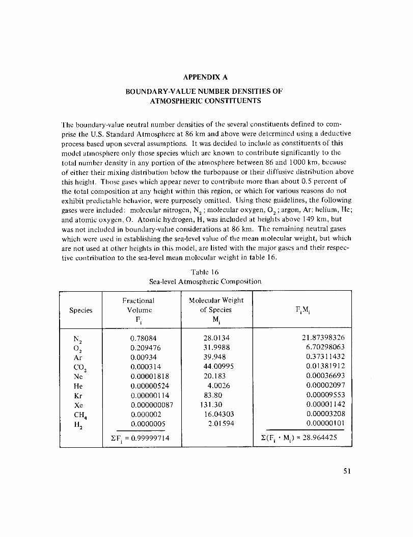
APPENDIXA
BOUNDARY-VALUE NUMBER DENSITIES OF
ATMOSPHERIC CONSTITUENTS
The boundary-value neutral number densities of the several constituents defined to com-
prise the U.S. Standard Atmosphere at 86 km and above were determined using a deductive
process based upon several assumptions. It was decided to include as constituents of this
model atmosphere only those species which are known to contribute significantly to the
total number density in any portion of the atmosphere between 86 and 1000 kin, because
of either their mixing distribution below the turbopause or their diffusive distribution above
this height. Those gases which appear never to contribute more than about 0.5 percent of
the total composition at any height within this region, or which for various reasons do not
exhibit predictable behavior, were purposely omitted. Using these guidelines, the following
gases were included: molecular nitrogen, N 2 ; molecular oxygen, 02 ; argon, Ar; helium, He;and atomic oxygen, O. Atomic hydrogen, H, was included at heights above 149 kin, but
was not included in boundary-value considerations at 86 km. The remaining neutral gases
which were used in establishing the sea-level value of the mean molecular weight, but which
are not used at other heights in this model, are listed with the major gases and their respec-
tive contribution to the sea-level mean molecular weight in table 16.
Table 16
Sea-level Atmospheric Composition
Species
N 2
OzAr
CO 2Ne
He
Kr
Xe
CH 4
H 2
Fractional
Volume
F.I
0.78084
0.209476
0.00934
0.000314
0.00001818
0.00000524
0.00000114
0.000000087
0.000002
0.0000005
NF. = 0.999997141
Molecular Weight
of Species
M i
28.0134
31.9988
39.948
44.00995
20.183
4.0026
83.80
131.30
16.04303
2.01594
F i M i
21.87398326
6.70298063
0.37311432
0.01381912
0.00036693
0.00002097
0.00009553
0.00001142
0.00003208
0.00000101
N(F i • Mi)= 28.964425
51

Thefirst threeof thegasesusedin thismodelcomprisemorethan0.9996 of the air in any
unit volume at sea level, as is evident from summing the fractional composition F i over
these three species in table 16. Since the fractional volumes of these major species do not
change significantly below the mesopause, which in this model is located at 86-km altitude,
the sea-level fractional composition can be assumed to be approximately correct at 86 km.
It is believed, however, that photochemical processes lead to small quantities of atomic
oxygen in this height region, and a fractional amount of about 0.00059 by volume, or
exactly 8.6 X 10 _6 atoms per m 3 , was agreed upon by Task Group II as an acceptable con-
centration of O for 86 km.
The introduction of the fixed amount of atomic oxygen at this height, and the simultane-
ous elimination of some minor species made it necessary to adjust the fractional concen-
trations of each of the four remaining species from their known sea-level values, F i, by acommon unknown factor, e, to the 86-km fractional composition values, F' such that
i '
F Ii 6 • F i (58)
The 86-km fractional composition of atomic oxygen is equal to the ratio of n(O) to N,
where n(O) is equal to 8.6 X 10 _6 m3 , the adopted atomic-oxygen number density for
that height, and N is the unknown total number density at that height. The sum of the
86-km fractional composition of the remaining four species is
Z F.S = e "Z Fi1
4 4
(59)
The sum of the total of the 86-km fractional compositions, (that is, of the five species
adopted to comprise the model at this height) must equal unity in accordance with the
expression:
_, n(O)6. F i +N
4
-1 (60)
The total number density, N, is expressible in terms of the mean molecular weight, M,
Avogadro's constant, NA , and the mass density, p, the value of which is known at 86 km
from other considerations. This relationship is
N A • pN - (61)
M
The mean molecular weight at 86 km is the sum of the products F'i ° Mi over the five gases
comprising the model at this height. For the atomic oxygen this product is
F'(O).M(O) = n (O)'M(O) (62)N
52
whilethesumof theproductsof theremainingfour gasesisexpressibleas
S F_ Mi = £ "S Fi Mi
4 4
(63)
such that the mean molecular weight, M, at 86 km is expressed as
ZM = e. Fi'Mi + (64)N
4
Eliminating M between equations 61 and 64, and solving for e yields
NA" p - n (O)'M (0)E = (65)
N "_--_, Fi.Mi
4
The elimination of e between equations 60 and 65 leads to the following expression for
total number density:
(_Fi)'[NA "P-n(O)'M(O)]
N - + n(O) (66)
Z F i • M i
4
From table 16 the value of _F i, the sum of F i for the four species N 2 , 02 , Ar, and He is
seen to be 0.99966124, while the value of 4_Fi M i for the same four species is seen to be
28.95009918. The value of M(O) is taken to be one half of the value of M(O 2 ), also givenin table 16. The value of 8.6 × 10¹⁶ m -3 was adopted for n(O), as previously stated, and
N A has the standard value 6.022169 × 1026 kmol q . The value of p at 86 km is found tobe 6.957880 × 10.6 kg/m 3 . These values, introduced into equation 66, yield a number
density of 1.447265 × 10²⁰ m3 at 86 km. This value introduced into equation 58 leads
to e = 0.99974445, while equation 64 then yields M = 28.952208 for the molecular weight
at 86 km.
For the 86-km height, the values of F'i, the fractional composition of each of the five spe-
cies comprising the model at that height, are given in table 17 as the product e • F'i, along
with the corresponding products F'i " Mi' and the corresponding values of N • F'i, the num-
ber densities of the five gas species comprising the model atmosphere at 86-km height.
The value of sZF[, the sum of the five values of F[ listed in table 17 is seen to be 0.999999999,essentially the unity value which it should have. The sum of the five values of F! • M. and
1 1
of the five values of n i, that is, sZF; • M'i and 5_ni, both of which are also given in table 17,shows essentially exact agreement with the value of their respective equivalents, M and N,
computed independently. Thus, the validity of the computation is established.
53

Table17NumberDensitiesandMolecularWeightat 86km
N 2
02Ar
He
O
F_ = eF. F' = F_, 1 i " mi (kg/kmol) n i , • N (m "3)
0.7806404557
0.2094224682
0.00933761315
0.00000523866
0.00059422421
Z F_ = 0.9999999999251
21.86839334
6.701267675
0.3730189704
0.0000209683
0.0095072308
NF_-M. = 28.952208251 !
1.129793736 × 10²⁰
0.3030898426 X 10²⁰
0.0135140022 X 10²⁰
0.0000075817 X 10²o
0.00086 X 10²⁰
Zn.=1.447265163 × 10205 i
54

APPENDIXB
A SEGMENTOFAN ELLIPSE TO EXPRESS
TEMPERATURE VERSUS HEIGHT
It is desired to determine the expression for a temperature function for a limited height
region, Z_ = 91 to Z 9 = 110 km, in the plane defined by Z and T, such that the slope of
the function at each of the end points exactly matches a prescribed value. At Z = Z 8 ,
where T = T 8 = 186.8673 K, the derivative of the function with respect to Z must be zero,
to match the slope of the temperature-height profile in the isothermal layer between 86
and 91 km. At Z = Z9, where T = T 9 = 240 K, the derivative of T with respect to Z must
be 12 K/km to match the slope of a layer of constant temperature-height gradient between
110 and 120 km. A suitably adjusted ellipse will satisfy these conditions.
The general equation of an ellipse in terms of Z and T with center at Z = 0 and T = 0 is
Z 2 T 2+ -- = 1 (67)
a 2 A2
With the center shifted to Z = Zc and T = T c the expression becomes
(Z- Ze)2 (T- Te)2+ - 1 (68)
a2 A2
The derivative of equation 68 with respect to Z is
2(Z - Ze) 2(T- T) dT+ .--= 0 (69)
a 2 A 2 dZ
To meet the condition for dT/dZ = 0 at Z = Za, equation 69 is evaluated for those condi-
tions, and it is found that Z c = Z s , such that equation 68 may be rewritten as
(z-zs) (T-Tc)2
a 2 A 2
-1 (70)
Evaluating equation 70 for Z = Z 8 and T = T 8 leads to
A = Ts - T (71)
Substituting Z c for its equal Z a in equation 69, and evaluating that expression for Z = Zg,
where T = T 9 and where (dT/dZ) has the particular value LK, 9 = 12, and finally solvingthe resulting expression for 1/a 2 yields
55

1 - (T9 - Te)'LK,9
a 2 A2.(Z 9 - Zs)(72)
Evaluating equation 70 at Z = Z9, where T = T9, and solving for 1/a 2 yields
1 A2 _ (T 9 _ Tc )2
a 2 A2.(Z9 - Z8)
(73)
Eliminating 1/a 2 between equations 72 and 73, and solving for T c leads to
LK, 9 "(Z 9-Z8)" T 9+T 2-r 2
Te = LK,9 "(Z9-Z8 ) +2T8-2T9(74)
The elimination of A between equations 71 and 73 yields
(Z 9 - Zs).(T 8 - To)a = (75)
[(T8 _ To)2 _ (T 9 _ ,re)2] 1/2
Finally, solving equation 70 for T yields the functional expression
T(Z) = Te + A'I1 - (Z -Zs)211/2.a (76)
The evaluation of equations 71, 74 and 75, in accordance with Z s = 91 km, Ts = 186.8673 K,
Z9 = 110 kin, T 9 = 240 K, and LK, 9 = 12 K/kin, yields the following values for the threeconstants in equation 76"
T = 263.1905KC
A=- 76.3232K
a = - 19.9429 km
Since it was shown that Zc = Z s , the ellipse which meets the required derivative and temp-
erature conditions, has its center at Z = 91 km and T = 263.1905 K, and equation 76 repre-
sents the function which meets the required conditions.
56

APPENDIXC
GEOPOTENTIAL AND MOLECULAR-SCALE TEMPERATURE
The concept of geopotential as a measure of height was introduced by Bjerknes et al. (1910)
who, according to Harrison (1954), made use of the term dynamic height in referring to
the geopotential of a point because in meteorology, geopotential is preferable to geometric
height as a representation of the vertical coordinate of the point. Bjerknes proposed the
term geodynamic meter (gdm), or dynamic meter for short, as the name of the unit of
dynamic height. With a slight revision in the definition of this concept, the Aerological
Commission of the International Meteorological Organization in 1947 adopted the geo-
potential meter (gpm) defined such that 1 gpm = 0.98 gdm = 9.8 m 2/s 2 . This definition
related the geopotential meter directly to the sea-level value of the acceleration of gravity.
In the U.S. Standard Atmosphere of 1955, published in NACA Report 1235 (1955), the
standard geopotential meter (sgpm) was defined in terms of the so-called standard sea-level
value of the acceleration of gravity, 9.80665 m/s 2 , such that 1 sgpm = 9.80665 m 2/s 2 .
The use of the standard geopotential meter (now designated as m') was continued in tile
Air Research and Development Command (ARDC) Model Atmosphere, 1956 (Minzner
and Ripley, 1956); in the U.S. Extension to the ICAO Standard Atmosphere (Minzner et al.,
1958); in the ARDC Model Atmosphere, 1959 (Minzner et al., 1959), in the U.S. Standard
Atmosphere, 1962 (COESA, 1962); as well as in the 1975 revision of that Standard Atmo-
sphere (COESA, 1975). Implicitly, geopotential has been used as a measure of height in
all standard and model atmospheres, in which the tabulated values of atmospheric proper-
ties have been calculated on the basis of a value of the acceleration of gravity which is in-
variant with height.
The numerical value of the height of a particular point above sea level, in regions where
the sea-level value of the acceleration of gravity is equal to or less than 9.80665 m/s 2 , is
smaller when expressed in geopotential than when expressed in geometric meters. One
standard geopotential meter is exactly equal to one geometric meter only under very spec-
ialized and perhaps hypothetical conditions. These conditions involve the existence of a
region with a gravitational-field value of exactly 9.80665 m/s 2 (generally near the earth's
surface), and with a zero vertical gradient of that field over a height interval of at least one
geometric meter. The concept of 1 m' is more precisely defined, however, in terms of a
specific change in potential energy of a unit mass, such that 1 m' is exactly the height
increment through which one must lift one kilogram (mass) in order to increase its poten-
tial energy by 9.80665 J. The geometric equivalent of this height increment is essentially
one geometric meter (m) at sea level, but increases to more than 1 m with increasing height,
in a manner inversely proportional to the corresponding decrement of the acceleration of
gravity.
57
Theconceptof geopotentialhassomeverymeaningfulusesin meteorologyandaeronomy.Oneof its principaladvantagesis thereductionfrom 4 to 3 of thenumberof variablesinthehydrostaticequationwhengeopotentialis introduced.This featureis particularlyde-sirablein expressionsinvolvingthe integratedformsof thehydrostaticequation.Thus,theuseof thisconcept,eitherimplicitly or explicitly in thedefinitionof standardatmospheresproducedprior to thedevelopmentof high-speeddigitalcomputers,simplifiedthedefiningequationsandreducedthework involvedin manualcomputationof therelatedtables.Theuseof geopotentialhasbeenmaintainedin all subsequentstandardatmospheresinorderto avoidanyrevisionof the lowerportionof thetableswhichhaverepresentedtheestablishedstandardfor thepast50years.
Theintroductionof theconceptof molecular-scaletemperature,TM, cameat atimewhenstandard-atmospheretableswerebeingextendedto heightswherethecomposition,andhencethemeanmolecularweight,wereunknown.Theconcept(without aparticularname)wasfirst appliedto atmosphericmodelsby theRocketPanel(1952)in apaperwhichre-ferredto a"derived'Temperature'baseduponanassumedconstantmeanmolecularweightp of 28.966 g/mole for the atmosphere." The use of this special kind of temperature not
only avoided the problem of determining or guessing at a value of mean molecular weight
at high altitudes, but also eased the problem of hand or desk-computer calculations by
leading to simpler equations than would have resulted if specific height functions had been
introduced for both kinetic temperature and mean molecular weight.
The name molecular-scale temperature for this derived temperature first appeared in the
ARDC Model Atmosphere, 1959. In this model, molecular-scale temperature, T M, at any
height Z was related to the kinetic temperature, T, at height Z by the relationship T M(Z)
= T(Z) [M0/M(Z)] where M0 was the currently accepted sea-level value of the mean mole-
cular weight of air, 28.9644 kg/kmol, and M was the implicit value of the mean molecular
weight of air at height Z. This concept was carried into the U.S. Extension to the ICAO
Standard Atmosphere, 1958; the ARDC Model Atmosphere, 1959; the U.S. Standard Atmo-
sphere, 1962 (COESA, 1962), and has been carried into the 1975 revision to that Standard
Atmosphere (COESA, 1975).
The temperature-height profile of each of the first three of these four previously published
models was defined in terms of T M (in units of Kelvin, K) as a function of geopotential
height H (in units of m') Over the entire height range of these models. Since many aerono-
mers studying the upper atmosphere are unfamiliar with these quantities and prefer the
quantities kinetic temperature, T, and geometric heights, Z, it was decided that, in the
US. Standard Atmosphere, 1962 (COESA, 1962) the model should be divided at 90 geo-
metric kilometers, with temperatures in that part of the model from 0 to 90 km defined in
terms of T M and H, and in that part above 90 km defined in terms of T and Z. This proce-dure has been continued in the t975 U.S. Standard Atmosphere, but in this revision, the
division occurs at 86 geometric kilometers where the geopotential is 84.8520 km', and
M = 28.9522 kg/kmol.
58
Beforethenamemolecular-scaletemperaturewasusedin modelatmospheres,Brombacher(1953),in anattemptto simplifythecalculationof standardatmospheres,combinedtheheight-dependentaccelerationof gravity,theheight-dependentmolecularweight,andtheheight-dependentkinetictemperatureinto asinglevariable,whichhecalledscale-heighttemperature.Theuseof thisvariable,howevermeritorious,wasneveradoptedin U.S.StandardAtmospheres.
REFERENCES
Bjerknes, V. et al., Dynamical Meteorology and Hydrography, 1, Washington, D.C., 1910.
Brombacher, W. G., "Proposed Standard Atmosphere to 160 km (500,000 ft)," National
Bureau of Standards, NBS Report 2680, 1953.
COESA (Committee on Extension to the U.S. Standard Atmosphere), U.S. Standard A tmo-
sphere, 1962, Government Printing Office, Washington, D.C., 1962.
COESA, U.S. Standard Atmosphere, 19 75, Government Printing Office, Washington, D.C.,
1975, in press.
Harrison, "Relation Between Geopotential and Geometric Height," Smithsonian Meteoro-
logical Tables, List, R. J., ed., Washington, D.C., 1954, p. 217.
Minzner, R. A. and W.S. Ripley, "ARDC Model Atmosphere, 1956," Air Force Surveys in
Geophysics, 86, AFCRC TN-56 204, 1956.
Minzner, R. A., W. S. Ripley, and T. P. Condron, U.S. Extension to the ICAO Standard
Atmosphere, Government Printing Office, Washington, D.C., 1958.
Minzner, R. A., K. S. W. Champion, and H. L. Pond, "The ARDC Model Atmosphere, 1959,"
Air Force Surveys in Geophysics, 155, AFCRC-TR-59-267, 1959.
Rocket Panel, "Pressure Densities and Temperature in the Upper Atmosphere," Phys. Rev.,
88, 1952, pp. 1022-1032.
Standard Atmosphere - Tables and Data for Altitudes to 65,800 ft., NACA Report 1235,
1955.
59

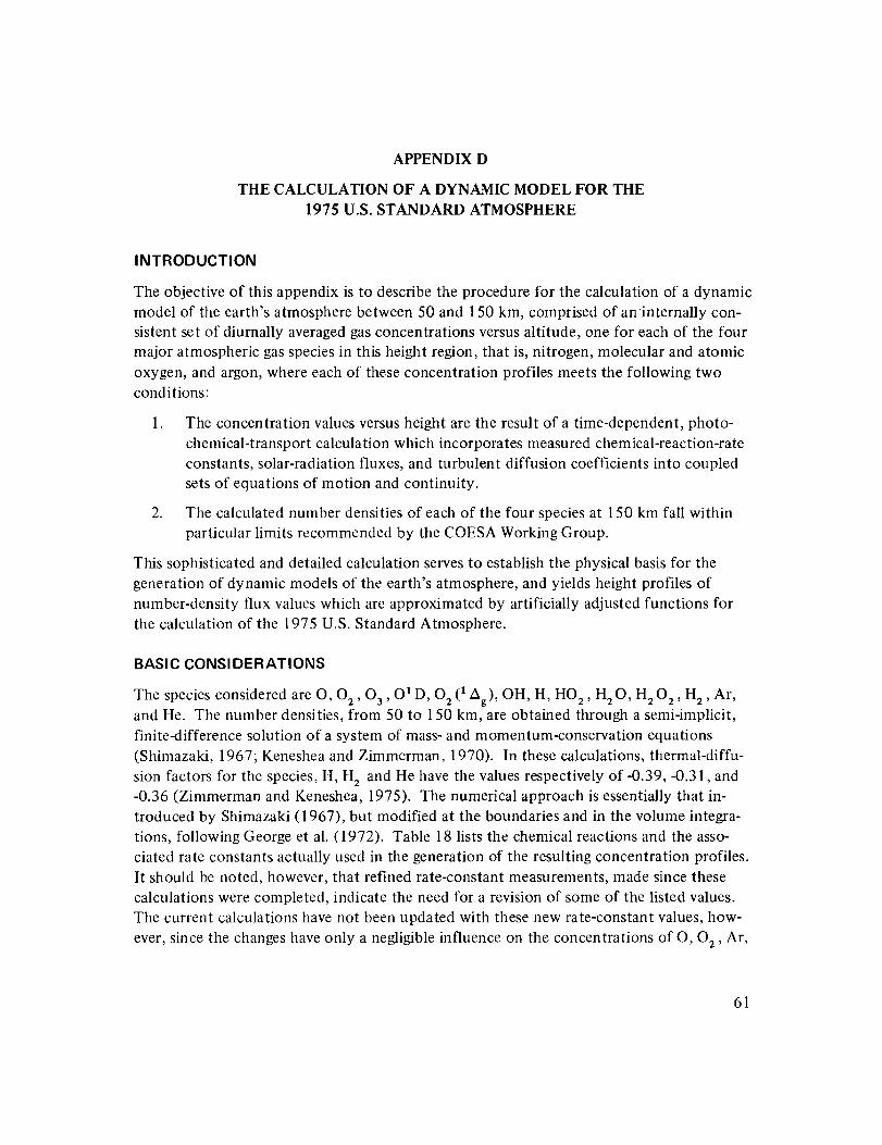
APPENDIXD
THE CALCULATION OF A DYNAMIC MODEL FOR THE
1975 U.S. STANDARD ATMOSPHERE
INTRODUCTION
The objective of this appendix is to describe the procedure for the calculation of a dynamic
model of the earth's atmosphere between 50 and 150 km, comprised of an internally con-
sistent set of diurnally averaged gas concentrations versus altitude, one for each of the four
major atmospheric gas species in this height region, that is, nitrogen, molecular and atomic
oxygen, and argon, where each of these concentration profiles meets the following two
conditions:
1. The concentration values versus height are the result of a time-dependent, photo-
chemical-transport calculation which incorporates measured chemical-reaction-rate
constants, solar-radiation fluxes, and turbulent diffusion coefficients into coupled
sets of equations of motion and continuity.
2. The calculated number densities of each of the four species at 150 km fall within
particular limits recommended by the COESA Working Group.
This sophisticated and detailed calculation serves to establish the physical basis for the
generation of dynamic models of the earth's atmosphere, and yields height profiles of
number-density flux values which are approximated by artificially adjusted functions for
the calculation of the 1975 U.S. Standard Atmosphere.
BASIC CONSI DERATIONS
The species considered are O, 02 , 03 , O =D, 02 (1 Ag), OH, H, HO 2 , H20, H202 , H 2 , Ar,and He. The number densities, from 50 to 150 km, are obtained through a semi-implicit,
finite-difference solution of a system of mass- and momentum-conservation equations
(Shimazaki, 1967; Keneshea and Zimmerman, 1970). In these calculations, thermal-diffu-
sion factors for the species, H, H 2 and He have the values respectively of-0.39, -0.31, and-0.36 (Zimmerman and Keneshea, 1975). The numerical approach is essentially that in-
troduced by Shimazaki (1967), but modified at the boundaries and in the volume integra-
tions, following George et al. (1972). Table 18 lists the chemical reactions and the asso-
ciated rate constants actually used in the generation of the resulting concentration profiles.
It should be noted, however, that refined rate-constant measurements, made since these
calculations were completed, indicate the need for a revision of some of the listed values.
The current calculations have not been updated with these new rate-constant values, how-
ever, since the changes have only a negligible influence on the concentrations of O, 02 , Ar,
61
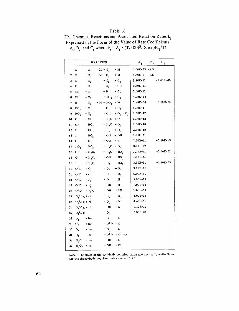
Table18TheChemicalReactionsandAssociatedReactionRateskjExpressedin theFormof theValueof RateCoefficients
Aj, Bi,andCj whereki = Aj • (T/300)BJX exp(Ci/T)
REACTION Aj Bj C i
1 O _O +M_O2 +M
2 O dO 2 +M_O 3 _M
3 O + O 3 ' O 2 + O 2
4 H + O 3 _ O 2 + OH
5 OH + O _ H + O 2
6 OH +O 3 - HO2 + O2
7 H + 02 + M _ HO 2 + M
8 HO 2 40 -. OH + 02
9 HO 2 +O 3 -_OH +O 2 +O_
10 OH +OH _ H20 +O
11 OH + HO 2 '" H20 + 02
12 H + HO 2 _ H 2 + 02
13 H + HO 2 ' OH + OH
14 O + H 2 _ OH + H
15 HO 2 + HO 2 _ H202 ÷ 02
16 OH + H2O 2 -" H20 + HO 2
17 O + H202 - OH + HO 2
18 H + H202 _ H 2 + HO2
19 01 D + 03 " 02 + 02
20 O l D + 02 _ O + 02
21 OID + N 2 _ O + N 2
22 OID + H 2 - OH + H
23 O tD + I{20 _ OH + OH
24 O2tAg+ O 3 _O 2 +03
25 O21Ag-_ M _ 02 + M
26 O2tAg+ H _ OH +O
27 O2 tAg _ 02
28 02 + hv _ O + O
29 02 + hv - O l D + O
30 03 + hv _ 0 2 + O
31 0 3 +by -OlD +O21:_g
32 H20 +hv - OH + H
33 H202 +hv - OH +OH
3.00E-33
5.50E-34
1.20E-If
2.60E-n
5.00E-11
4.00E-14
7.40E-33
1.00E-11
1.00E-17
2.00E-12
2.00E-10
3.00E-12
1.00E-11
7.00E-11
3.00E-12
1.70E-11
4.00E-15
3.90E-11
3.00E-10
6.00E-11
9.00E-11
1.00E-11
1.00E-11
3.00E-15
4.40E-19
1.10E-14
2.58E-04
-2.9
-2.6
-2.00E+03
6.10E+02
-5.10E+03
-9.00E+02
-4.60E+03
Note: The units of the two-body reaction rates are cm 3 s-', while those
for the three-body reaction rates are cm 6 s "1.
62

andHein the altitude region above 80 km. The intensity of the solar-radiation flux used
in these calculations is 0.65 of that shown in figure 17, which depicts the Ackerman ( 1971 )
values of solar-radiation flux versus wavelength. The absorption cross sections were taken
from various sources. For 02 and 03 , these cross sections were taken from the compila-tion of Ackerman (1971) with the exception of those for the Schumann-Runge bands of
02 , for which region the values measured by Hudson and Mahle (1972) were used. Theadopted absorption cross sections for water vapor and hydrogen peroxide are those re-
ported by Watanabe and Zelikoff (1953), and by Volman (1963), respectively. The temp-
erature-height profile up to 150 km and the values of mean molecular weight up to the
turbopause are those recommended by the Working Group of COESA. Using these data,
the initial species distributions were calculated assuming complete mixing up to the turbo-
pause, and diffusive equilibrium above it.
101 _,
1014
1013
low _=
o 10 H
xD
J 101o
0
_ 10 _
10 a
110
SOLAR FLUX
i I [ I 1 I 1 i I
HLva
I 1 I I I I I 1 I
130 150 170 190 210 230 250 270 290 310
WAVELENGTH, nm
Figure 17. Solar radiation flux versus wavelength in the region
from 115 to 310 nm as reported by Ackerman.
The total number density was obtained by integrating the hydrostatic equation, where the
sea-level values of mass density and of mean molecular weight were taken from the U.S.
Standard Atmosphere, 1962 (COESA, 1962).
Beginning with these static profiles, the steady-state solution of all species was determined.
The time-dependent calculations were then allowed to proceed for 15 solution days using
a semi-implicit, finite-difference technique, a variable-time step up to 30 minutes, and a
fixed-height step of 100 m. This stringent height step was shown to be necessary to restrict
the errors generated by species gradients when height steps larger than 100 m were used.
63

The height-dependent, turbulent diffusion coefficients used are shown in figure 18, and
are based upon observations of turbulence in chemical trails (Philbrick et al., 1973). These
values are derived (Zimmerman and Trowbridge, 1973) from the fluctuation dynamics ob-
served in rocket-borne chemical releases, and are valid from about 88 to 112 km. Because
of the lack of chemical-tracer wind and turbulence measurements in the altitude region
between 50 and 88 km, an exponential fit has been assumed between the reported value
of 1 × l0 s cm 2 sl (Beaudoin et al., 1967) at 50 km, and the values at 88 km.
El
aD
150
140
130
120
110
100
9O
i I ! ! I I II [ I ! I I I 1 I1 [ ! ! I ! I I T !
J
80
70
60
5o , i , , , ,,,I101 10 2 I0 3
EDDY -- DIFFUSION COEFFICIENT, m2/s
I I I I I III
10 4
Figure 18. Eddy-diffusion coefficient versusaltitude.
RESULTS
The time-dependent calculations were continued for the above mentioned period of time,
after which the species concentrations reproduced themselves to within 1 percent over a
diurnal cycle, a condition which is called arriving at diurnal reproducibility. The diurnal
averages of the concentration of O, 02 , and Ar are then calculated and extrapolated to
250 km by assuming diffusive equilibrium without thermal diffusion above the 150-km
boundary. Figure 19, depicting the height profiles of the N 2 concentration and tempera-
ture, shows the initial conditions used in these one-dimensional calculations. Figure 20
shows the resulting diurnally averaged height profiles of O, 02 , and Ar, each of which is in
good agreement with the 150-km values recommended by the COESA Working Group, and
shown as error bars.
64

E
5<
10 TM
250
240
230
22O
210
2O0
190
180
170
160
150
140
130
120
110
100
9O
80
70
60
5O
100
N2 CONCENTRATION, m "3
1015 1016 1017 1018
i i i i i
i.-.1
1019 1020 1021 1022 1023
1
200 300 400 500 600 700 800 900 1000
TEMPERATURE, K
I I I I
Figure 19. Altitude profile of kinetic temperature and molecular nitrogen concentration
with the range of 150-km values recommended by the COESA Working Group indicated
by an error bar.
290
270
250
230
210
E 190
wQ 170
150
........ I ........ I ........ I ........ I ........ I ........ I ........
4
130
110
9O
7O
5O
Ar Z¸
1014 101_ 1016 1017 10l_ 10 I_ 1020
CONCENTRATION, ,n _
Figure 20. Altitude profiles of diurnally-averaged concentrations of O, 02, and Ar,
with the range of 150-kin values recommended by the COESA Working Group indicated
by corresponding error bars.
65

Thus, it has been demonstrated that an internally self consistent model of the density struc-
ture of the upper mesosphere and lower thermosphere may be calculated from measured
values of solar radiation flux, chemical-reaction-rate constants, and derivatives of measured
vertical-turbulent-transport parameters deduced from chemical-trail studies.
REFERENCES
Ackerman, M., "Ultraviolet Solar Radiation Related to Mesospheric Process," Mesospheric
Models and Related Experiments, Fiocco, G., ed., Springer-Verlag, New York, 1971,
pp. 149-159.
Beaudoin, P. E., D. Golomb, T. M. Noel, N. W. Rosenberg, and W. K. Vickery, "Observa-
tion of Mesospheric Winds and Turbulence with Smoke Trails," J. Geophys. Res., 72,
1967, pp. 3729-3733.
COESA (Committee on Extension to the U.S. Standard Atmosphere), U.S. Standard Atmo-
sphere, 1962, Government Printing Office, Washington, D.C., 1962.
George, J. G., S. P. Zimmerman, and T. J. Keneshea, "The Latitude Variation of Major and
Minor Neutral Species in the Upper Atmosphere," Space Res., XII, Bowhill, S. A., et al.,
ed., Akademie-Verlag, Berlin, 1972, pp. 695-709.
Hudson, R. D. and S. H. Mahle, "Photodissociation Rates of Molecular Oxygen in the Meso-
sphere and Lower Thermosphere," J. Geophys. Res., 77, 1972, pp. 2902-2914.
Keneshea, T. J. and S. P. Zimmerman, "The Effect of Mixing upon Atomic and Molecular
Oxygen in the 70-170 km Region of the Atmosphere," J. A tmos. Sci., 27, 1970, pp. 831-
840.
Philbrick, C. R., R. S. Narcisi, R. E. Good, H. S. Hoffman, T. J. Keneshea, M. H. MacLeod,
S. P. Zimmerman, and B. W. Reinisch, "The ALADDIN Experiment, Part II - Composi-
tion," Space Res., XIII(1), Rycroft, M. J., and S. K. Runcorn, ed., Akademic-Verlag,
Berlin, 1973, pp. 441-448.
Shimazaki, T. J., "Dynamic Effects on Atomic and Molecular Oxygen Distribution in the
Upper Atmosphere: A Numerical Solution to Equations of Motion and Continuity,"
J. Atmos. Terr. Phys., 29, 1967, pp. 723-741.
Volman, D. H., "Photochemical Gas Phase Reactions in the Hydrogen Oxygen System,"
Advances in Photochemistry, 1, Interscience Publishers, N.Y., 1963, pp. 43-81.
66

Watanabe,K. andM.Zelikoff, "AbsorptionCoefficientsof WaterVaporin theVacuumUltraviolet,"Opt. Soc. Am. J., 43, 1953, pp. 753-755.
Zimmerman, S. P. and C. A. Trowbridge, "The Measurement of Turbulent Spectra and
Diffusion Coefficients in the Altitude Region 95 to 110 km," Space Res., XIII(1 ),
Rycroft, M. J. and S. K. Runcorn, ed., Akademie-Verlag, Berlin, 1973, pp. 203-298.
Zimmerman, S. P. and T. J. Keneshea, "The Thermosphere in Motion," (submitted for
publication), J. Geophys. Res., 80, 1975.
NASA-Langley, 1976 67


NATIONAL AERONAUTICS AND SPACE ADMINISTRATION
WASHINGTON. D.C. 2.0546
OFFICIAL BUSINESS
p .................. E =3oo SPECIAL FOURTH-CLASS RATE
BOOK
POSTAGE AND FEES PAID
N&TIONAL AERONAUTICS AND
SPACE ADM _NiSTRATION
451
POSTMASTER:If Undeliverable (Section 158
Postal Manual) Do Not Return
"The aeronautical and space activities of the United States shall becomtucted so as to contribute . . . to the expansion o[ human knowl-edge o[ phenomena in the atmosphere and space. The Administrationshall provide for the widest practicable and appropriate disseminationo[ information concerning its activities and the results thereo[."
--NATIONAL AERONAUTICS AND SPACE ACT OF 1958
NASA SCIENTIFIC AND TECHNICAL PUBLICATIONS
TECHNICAL REPORTS: Scientific and
technical information considered important,
complete, and a lasting conrribution to existing
knowledge.
TECHNICAL NOTES: Information less broad
in scope but nevertheless of importance as a
contribution to existing knowledge.
TECHNICAL MEMORANDUMS:
Information receiving limited distribution
because of preliminary data, security classifica-tion, or other reasons. Also includes conference
proceedings with either limited or unlimiteddistribution.
CONTRACTOR REPORTS: Scientific and
technical information generated under a NASA
contract or grant and considered an important
contribution to existing knowledge.
TECHNICAL TRANSLATIONS: Information
published in a foreign language considered
to merit NASA distribution in English.
SPEC1AL PUBLICATIONS: Information
derived from or of value to NASA activities.
Publications include final reports of major
projects, monographs, data compilations,
handbooks, sourcebooks, and special
bibliographies.
TECHNOLOGY UTILIZATION
PUBLICATIONS: Information on technology
used by NASA that may be of particular
interest in commercial and other, non-aerospaceapplications. Publications include Tech Briefs,
Technology Utilizati_m Reports and
Technology Surveys.
Details on the availability of these publications may be obtained from:
SCIENTIFIC AND TECHNICAL INFORMATION OFFICE
NATIONAL AERONAUTICS AND SPACE ADMINISTRATION
Washington, D.C. 20546