NASA-CR-198957

NASA GRANT REPORT

&'_W> ":.''

c;'s J/ ,_ --l

NASA GRANT NAG8-1041

ENHANCEMENTS TO THE SSME TRANSFER FUNCTION MODELING CODE

Prepared by:

R. Dennis Irwin

Jerrel R. Mitchell

David L. Bartholomew

Russell D. Glenn

On behalf of:

Department of Electrical and Computer EngineeringCollege of Engineering and Technology

Ohio University

Athens, Ohio 45701

July 1995

(NASA-C_-I98957) ENHANCEMENTS TOTHE SSME TRANSFER FUNCTION MODELINGCO0:E Interim Report (Ohio Univ.)59 p

N95-30754

Uncl.as

G3/64 0056456

Interim Report

Prepared for:

NASA George C. Marshall Space Flight Center

Marshall Space Flight Center, Alabama 35812

https://ntrs.nasa.gov/search.jsp?R=19950024333 2018-06-18T22:21:41+00:00Z

- i

1.0

2.0

2.1

2.1.1

2.1.1.1

2.1.1.2

2.1.1.3

2.1.2

2.1.3

2.1.3.1

2.1.3.2

2.1.3.3

2.2

2.2.1

2.2.2

2.3

2.4

2.4.1

2.4.2

2.4.3

2.4.3.1

2.4.3.2

3.0

3.1

3.2

3.3

3.4

3.5

4.0

5.0

5.1

5.2

6.0

TABLE OF CONTENTS

INTRODUCTION ........................................ 1

ANALYTICAL BACKGROUND ............................... 2

Derivation of Spectral Modeling Methods ..................... 2

Fundamental Relationships .......................... 2

Mean Value of Discrete Ergodic Data ............... 2

Covariance and Correlation of Discrete Ergodic Data ..... 3

Spectral Density Functions ...................... 4

Ideal Single Input/Single Output Relationships .............. 5

Non-Ideal Single Input/Single Output Relationships ........... 7

General Non-Ideal SIMO Relationships .............. 7

SIMO Relationships Useful in System Identification ...... 9

Motivation for Spectral Data Modeling-The Ratio Method 10

The Eigensystem Realization Algorithm (ERA) ................. 11

Theory and Description of ERA ...................... 11

Limitations of the Algorithm ........................ 14

Modeling Spectral Quantities Using ERA ..................... 15

The Residue Identification Algorithm ....................... 17Standard RID ................................. 17

Constrained Least Squares RID ...................... 20

Total Least Squares RID .......................... 21

Total Least Squares ......................... 21

Issues in Applying Total Least Squares to RID ........ 25

APPLICATION OF THE SSME TRANSFER FUNCTION MODELING CODE

TO EXPERIMENTAL DATA ................................ 27

A Straightforward Application ........................... 27

The Trending Method ........................ ......... 33

Filtering ......................................... 40

Eliminating Excitations ................................ 44Constrained RID .................................... 46

ENHANCEMENTS TO THE SSME CODE ....................... 48

ENHANCEMENTS TO XPLOT ..................... ......... 51

Additional Features .................................. 51

Possible Future Additions 51

CONCLUSIONS ........................................ 52

ii

6.16.2

Observationsand SummaryResults ........................ 52FutureWork ...................................... 53

7.0 REFERENCES ......................................... 55

o°°

111

1.0 INTRODUCTION

This report details the results of a one year effort by Ohio University to apply the

transfer function modeling and analysis tools developed under NASA Grant NAG8-167 (Irwin,

1992), (Bartholomew, 1992) to attempt the generation of Space Shuttle Main Engine High

Pressure Turbopump transfer functions from time domain data. In addition, new enhancements

to the transfer function modeling codes which enhance the code functionality are presented,

along with some ideas for improved modeling methods and future work.

Section 2 contains a review of the analytical background used to generate transfer

functions with the SSME transfer function modeling software. Section 2.1 presents the "ratio

method" developed for obtaining models of systems that are (1) subject to single unmeasured

excitation sources and (2) have two or more measured output signals. Since most of the models

developed during the investigation use the Eigensystem Realization Algorithm (ERA) for model

generation, Section 2.2 presents an introduction of ERA, and Section 2.3 describes how it can

be used to model spectral quantities. Section 2.4 details the Residue Identification Algorithm

(RID) including the use of Constrained Least Squares (CLS) and Total Least Squares (TLS).Most of this information can be found in the report (and is repeated for convenience).

Section 3 chronicles the effort of applying the SSME transfer function modeling codes

to the a51p394.dat and a51p1294.dat time data files to generate transfer functions from the

unmeasured input to the 129.4 degree sensor output. Included are transfer function modeling

attempts using five methods. The first method is a direct application of the SSME codes to thedata files and the second method uses the underlying trends in the spectral density estimates to

form transfer function models with less clustering of poles and zeros than the models obtained

by the direct method. In the third approach, the time data is low pass filtered prior to the

modeling process in an effort to filter out high frequency characteristics. The fourth method

removes the presumed system excitation and its harmonics in order to investigate the effects of

the excitation on the modeling process. The fifth method is an attempt to apply constrained RID

to obtain better transfer functions through more accurate modeling over certain frequency ranges.

Section 4 presents some new C main files which were created, to round out the

functionality of the existing SSME transfer function modeling code. It is now possible to go

from time data to transfer function models using only the C codes; it is not necessary to rely on

external software. The new C main files and instructions for their use are included.

Section 5 presents current and future enhancements to the XPLOT graphics program

which was delivered with the initial software. Several new features which have been added to

the program are detailed in the first part of this section. The remainder of Section 5 then lists

some possible features which may be added in the future.

Section 6 contains the conclusion section of this report. Section 6.1 is an overview of

the work including a summary and observations relating to finding transfer functions with the

SSME code. Section 6.2 contains information relating to future work on the project.

2.0 ANALYTICAL BACKGROUND

This section of the report contains the analytical background required to understand the

overall approach to identifying transfer functions estimates. The centerpiece algorithm is the

"ratio method" of determining transfer functions based on rational function or state-space models

of auto- and cross-spectra of two or more measured output signals.

Section 2.1 contains a complete derivation of the ratio method, including properties of

discrete-time random processes, their use in the analysis of linear systems, and their application

to the transfer function identification problem. Since the Eigensystem Realization Algorithm

(ERA) has been used extensively for identifying the linear models necessary in applying the ratio

method, Section 2.2 contains the details of using ERA to determine linear models given a system

pulse response, and Section 2.3 shows how ERA can be used to model spectral quantities.

Finally, Section 2.4 details the analytical background for the Residue Identification Algorithm

(RID) and various modifications of it based on Constrained Least Squares (CLS) and Total Least

Squares (TLS).

2.1 Derivation of Spectral Modeling Methods.

The method for identifying the characteristics of a system from models of the spectral

characteristics of its measured output signals relies heavily on the theory of random variables.

This section outlines the necessary theory. In Section 2.1.1, fundamental equations of random

variable theory are presented. These equations and theory are applied to an ideal single

input/single output system in Section 2.1.2. Finally, in Section 2.1.3, equations for non-ideal

(i.e., disturbances in measurements of output signals) single input/multiple output systems are

presented and developed. The equations in this section are presented for the discrete-time case.

Many of the developments closely parallel the continuous-time presentations found in Bendat and

Piersol (1980) and Cooper and McGillem (1971).

2.1.1 Fundamental Relationships.

In this section, a selection of useful relationships for discrete random variable analysis

is presented. These relationships form the foundation of the single input/single output and single

input/multiple output system theories that are developed in subsequent sections.

2.1.1.1 Mean Value of Discrete Ergodic Data.

Given an ensemble of discrete data records, xi(k) (i=1,2,...,n), representing

measurements of any single phenomenon of interest, it is possible to estimate the mean value

(Bendat and Piersol, 1980, p. 3) at any discrete point kl by averaging over the entire ensemble.

In equation form this is

2

t_x(kl) = lim 1 _ x,(k,) . (2.1.1)n--_ou n i.1

If the mean value and all other moments of interest, such as the mean square value, are constants

that are independent of their discrete origin, then the data is said to be stationary (Cooper and

McGillem, 1971, p. 177). In addition, if the data is assumed to be ergodic (Cooper and

McGillem, 1971, p. 179), then each member of the ensemble will exhibit the same statistical

behavior as the whole ensemble. For ergodic data the mean value may be computed by using

the equation 1 N-I#=lim _ _ x,(k) , (2.1.2)

N.-,o* 1¥ k=O

where N is the total number of data points in xi(k). This is equivalent to solving for the expected

value (Bendat and Piersol, 1980, p. 30) of any individual member of the ensemble xi(k).

2.1.1.2 Covariance and Correlation of Discrete Ergodic Data.

Consider two discrete data records, x(k) and y(k), of length N points each (i.e.,

k=0,1,2,...,[N-I]). Assuming identical sample rates, these data records can be represented by

the discrete time-domain functions x(kT,+tx) and y(kT,+O, respectively, where Ts is the sample

period and t, ant ty are the respective time origins when k=0. Defining a new variable r=ty-t,and assuming tx as the reference (i.e. assuming t,=0), these functions may be re-written as

x(kT,+t) l,.o = x(kT) (2.1.3)

and

y(kT,+QI,=,.-,, = y(kT,+r). (2.1.4)

The covariance function (Bendat and Piersol, 1980, p. 47) is a function of the time delay, r, and

it is defined as

--El{x(kT) {y(k7, l, (2.1.5)

where the symbol E represents the expected value of the indicated quantity. By completing the

inner multiplication and applying the rule for expectations of sums (the expected value of a sum

is equal to the sum of the expected values), Equation 2.1.5 may be re-written into the form

C_(r)=E[x(kT) y(kT,+r)]- E[x(kT) I_y] (2.1.6)

-E[lz_ y(kT, +r)] + E bx_/_y]

Assuming that the data is ergodic, this reduces to

C_:(r) = R_e(r) - #:y -/z:y +/x:y (2.1.7)

where

R_,(z)= E[x(kT,) y(kT,+r)]u-1 (2.1.8)

= lim --1 _ x(kT) y(kT, +0N-.,,o* N k--O

is the cross-correlation function (Bendat and Piersol, 1980, p. 47; Cooper and McGillem, 1971,

p. 207) between x(kTs) and y(kT,). For the special case when x(kTs) and y(kTs) represent the

same data (i.e. x(kT_)=y(kTs)) the covariance function is given by

C_,0.) =R_,(r) _#_ , (2.1.9)

where

=E[x(kT)1 _-x (2.1.10)

=V,m x(kr,)x(krs+oN-- l¥ k=0

is the autocorrelation function (Bendat and Piersol, 1980, p. 48; Cooper and McGillem, 1971,

p. 190) of x(kT,). An important property of the autocorrelation function which will be useful

in later developments is that it is an even function of its independent variable r, that is,

R_,0.) =R_,(__-) . (2.1.11)

The cross-correlation function is neither an even nor an odd function of _-, but it does possess

the property

R_(r) =R_,(-r) . (2.1.12)

2.1.1.3 Spectral Density Functions.

If the autocorrelation and cross-correlation functions are assumed to be discrete in

nature, i.e., having been calculated for a discrete set of time delays, r=k,T,, where k, is the set

of integers and T. is the period of the discrete variable r, then the spectral density functions may

be calculated via the double-sided z-transforms (Phillips and Nagle, 1984, p. 22) of the

appropriate correlation functions. The autospectral density function (Bendatand Piersol, 1980,

p. 50; Cooper and McGillem, 1971, p. 236), or autospectrum, may be calculated by taking the

double-sided z-transform of the discrete autocorrelation function R_,(k.T,),GO

S_,(z)=Z[R_,(kT)]= __, R_,(k,T,.)z -k" , (2.1.13)kr= - o_

where the symbol Z represents the double-sided z-transform of the indicated quantity.

Similarly, the cross-spectral density, or cross-spectrum (Bendat and Piersol, 1980, p. 50; Cooper

and McGillem, 1971, p. 259), may be calculated by taking the double-sided z-transform of the

cross-correlation function R._(k,T,),

Sxy(Z) =Z[Rxy(k T)l = __, R:,y(kT) z -k, (2.1.14)

4

Certainpropertiesof the spectral functions (Cooper and McGillem, 1971, p.236, p.259)

will be useful in later developments. These properties may be summarized as follows:

.

o

The autospectrum is a real, even function of frequency co. Given that z=e `r',

where s=a+joJ, this translates (with a = 0) into

_r S e-J_r) . (2.1.15)s (g ,)=

The cross-spectrum is a complex function whose real part is a even function of

frequency and whose imaginary part is an odd function of frequency. Following

the notational convention established above, this is written as

and

j_TRe[S_(e 9] =Re[S_(e-J"r)]

(2.1.16)

,oT =-lm[S.( ")] ,Im[S_y(e _ ")] e-J'_r (2.1.17)

where the notation Re and lm represents the real and imaginary parts,

respectively.

. Assuming real coefficients, the cross-spectrum from signal x to signal y is equal

to the complex conjugate of the cross-spectrum from signal y to signal x,

•,_r S e-J_r (2.1.18),)=

2.1.2 Ideal Single Input/Single Output Relationships.

Consider the discrete single input/single output (SISO) system shown in Figure 2.1.1.

For this system, h(k) represents the discrete pulse response. The discrete output signal, y(k),

x(k) th(k)l>Y(k)

Figure 2.1.1 Ideal SISO System.

may be calculated using the discrete convolution formula (Phillips and Nagle, 1984, p. 34)

y(k)= _ h(n)x(k-n) . (2.1.19)n=-O0

In the time-domain, the output signal may be described by the discrete-time function y(kT,+ty)

for k=0,1,...N. Assuming ty as reference (ty=0), this becomes y(kTs).

By using Equations 2.1.10 and 2.1.19 and constraining the period of z to be equal to

the period of the sampled system, T,=T_, it is possible to solve for a discrete autocorrelation

function of the output signal in terms of the discrete pulse response and the input signal. This

is,

RJ_ T)=_-Iy(kL)y([k+kjT)]1"-' [ - t - I

_°op,.-_ . l":-" . J- - I1 _-, I

= _ h(nl) E h(nz) I "-_]_--_x([k-n,]T)x([k+k.-n2]T )|n,=-o* n:-o* [ k=O j

(2.1.20)

Examination of the last bracketed element of Equation 2.1.20 reveals that it defines a discrete

autocorrelation function of x(kT,). Thus, Equation 2.1.20 may be reduced to

oo

Ryy(kT)= _ h(n,)_ h(n2)R=([k,-n2+n,]T). (2.1.21)_ll=t-Go Fllffi- O0

As stated in Equation 2.1.13, an equation describing the autospectrum may be found by taking

the double-sided z-transform of a discrete autocorrelation function. Applying this to the

autocorrelation function of Equation 2.1.21 yields

Syy(z)= _ I _ h(n,) __, h(n2)R_,(tk_-n2+n,]T) Z (k'-n'÷nt)z(n'-n')k=-_ .,=-_. ,_=-,_ (2.1.22)

= E h(nl )z-n' h(n2)z"_]_-, R_,([k_-n2+nl]T_)z_k'-"2+"')'nl=-oo nz=-_ k =-oo

which may be expressed in the simplified form

Syy(z) = H(l/z) H(z) S=(z) . (2.1.23)

A discrete cross-correlation function between the input and output signals may be found

by using Equations 2.1.8 and 2.1.19. By constraining T,=T,, this may be written as

R v(kT) = E[x(kT) y([k+glL)]

= 1 _ x(kT,) h(n) x([k+k,-nlT)N k=0 ,=-_

" l1 _-1 (2.1.24)= __,. h(n) __, x(kT)x([k+k -n]T)=- . k=O

= _ h(n)R_,(tk_-n]T).n ffi- O_

Applying the double-sided z-transform, as in Equation 2.1.14, yields

6

S_(z)= _ h(n)R_,([k-n]T) z<k'-_z "

= _ h(n)z" _ R,_([k,-n]T,)z (k'-"

= H(z) S_(z) .

(2.1.25)

2.1.3 Non-Ideal Single Input/Multiple Output Relationships.

In this section, a selection of spectral relationships for non-ideal single input/multiple

output systems (SIMO) is developed. In Section 2.1.3.1, general equations for the non-ideal

SIMO system are presented. In Section 2.1.3.2, spectral relationships that are particularly useful

for system identification purposes are developed. Finally, in Section 2.1.3.3, the motivation for

modeling spectral data is discussed.

2.1.3.1 General Non-Ideal SIMO Relationships.

Consider the non-ideal SIMO system shown in Figure 2.1.2. For this system, the di(k)

represent random disturbances. These disturbances are added to the actual system output

h2fk) Y2fk)

x(k) :+ +

+ _'+

i

!

!

' di(k )

h,(k) [ - ; y;(k)[

Figure 2.1.2 Non-Ideal SIMO System.

signals, yi(k), causing the measured system output signals, y[(k), to be

y[ (k) = yi(k) + di(k) . (2.1.26)

An equation describing the autospectrum of any actual system output signal may be found by

applying Equation 2.1.23,

7

Sy,_,(z) = Hi(I/z)H_(z)S_(z) . (2.1.27)

Also, an equation describing the cross-spectrum between the input signal, x(k), and any

actual output signal may be found by applying Equation 2.1.25,

Sxy,(z) = H,(z) S,,_(z) . (2.1.28)

A discrete cross-correlation function between any two measured output signals can be derived

from Equations 2.1.8, 2.1.10, and 2.1.26. By assuming the time lag 7=k,T,, this may be

written as

e,:,;(k.L)=_/(kL) y/([k+k.]:9]

=:{y,(k_)+a,(kr,)}{yj(tk+kj_)+d_(tk+k]:r)}]

= E[y,(kT) yj([k+k)]T,] + E[y,(kT) dj([k+k ]T)]

+ E[d,(kT) yj([k+k]T,] + E[d,(kT) dj([k+k ]T)]

= Ry_(kT,) + Ry_(kT) + Ra_(k,T,)+ Ra_(k,T,) • (2.1.29)

If the disturbances are assumed to be mutually uncorrelated (i.e. di(k) uncorrelated with dj(k)

for i_j) and uncorrelated with all other signals in the system, then Equation 2.1.29 may be

reduced to

Ry:,;(kr)=Ry_(_L)

= E[ y,(kT) y_([k+k ]T)]

._k_o1.___1_' h,(n,)x([k-n,]T,)] 1.o__ h,(n,)x([k+k-n,]T)]

" _ [ 1"-' ]=_=.... h,(n,)_= h_(n/[:_zV,.ox(tk-n,17")x(tk+_-njlL)lj

oo

: _ h,(ni) ___ hj(nj)R_(k-nffni).

nl=-oo _=-Qo

(2.1.30)

An equation describing the cross-spectrum of any two measured output signals may be

found by taking the double-sided z-transform of Equation 2.1.30,

Sy,,y/(z)= _ h(n,) h(ni)R,,_([k-nj+n,lT ) z_k'-"*'Oz _''-n_

k--_. ,,.-,, ,,.-_ (2.1.31)

: _ h(n,)z-'___ h(nj)z'___ R=([k.-nj+n,]T)z `'-''+"_ ,n_=-_ n?-o_ k=_-_

which may be expressed in the simplified form

8

Sy/y/(z) = Sy_(z) (2.1.32)

= Hi(llz)tlj(z)S,_(z).

A discrete autoeorrelation function for any measured output signal may be found by

applying Equations 2.1.8, 2.1.10, and 2.1.26. This is

• Ry;y:(kTs)= E[y[ (kT) y/([k+k,]T)]

=

= E[y,(kr) y,([k+k)]T,l + E[yi(kT ) d,(tk+k, lT)]

+ eta#L) y,(tk+k.lL]+ a,([k+k.lL)]

= Ry,y(kT) + Rya(k,T ) + Ra_(k,T ) + Rd,a(k,T), (2.1.33)

which may be reduced to

Ry[y/(k,T) = Ryy,(kT) + Rda(_T ) (2.1.34)

because of the assumed lack of correlation between disturbances and actual output signals.

Taking the double-sided z-transform of Equation 2.1.34 yields an equation describing

the autospectrum of any measured output signal,

Srty:(z) = Sy_(z) + Sad(z) . (2.1.35)

If it is assumed that there exists a large signal to noise ratio,

Sy_,(z)/Sad(z ) -> 1 , (2.1.36)

then the autospectrum of the measured output signal will be approximately equal to the

autospectrum of the actual output signal. In equation form this is written as

Sr:y:(z) -- Sr,(z ) . (2.1.37)

2.1.3.2 SIMO Relationships Useful in System Identification.

As stated in Section 2.1.1.3, autospectra are real, even functions of frequency. In other

words, they are symmetrical about the zero frequency axis. Because of this symmetry, it is

possible to express autospectra in a factored rational form. Applying this to the input

autospectrum yields

(2.1.38)S_,(z) = D,,(llz)Dx(z )

The z-domain input-to-output (I/O) transfer functions, Hi(z), may be expressed as a ratio

of two z-domain polynomials. If the system is assumed to be linear, then the denominator

9

polynomial, or system determinant, will be the same for each I/O transfer function. In equation

form this is

Ni(z) (2.1.39)

= ) ,where the roots of Ds(z) are the z-domain poles of the system and K_ represents a constant gain.

Combining Equations 2.1.27, 2.1.37, 2.1.38, and 2.1.39 yields a new expression

describing the autospectrum of any measured output signal

K_N,( llz)N,(z)N:,( llz)N_,(z) (2.1.40)--

D ,( llz)D ,(z)O_,( llz)Dx(z)

Solving Equation 2.1.27 for a relationship describing the input autospectrum yields

Sy_,(z) (2.1.41)

s,,(z)- n,(1/z)n,(z)

which may be combined with Equations 2.1.32, 2.1.37, and 2.1.39 to yield a new equation

describing the cross-spectrum between any two measured output signals

r, Kj_( llz)Nj(z)D ( llz)D ,(z)Sy, y/(z)

Sy/y/(Z) -_ K_Ni(1/z)Ni(z)D ,(1/z)D ,(z)

-_K,3V,(z)

Finally, Equation 2.1.42 may be manipulated into the form

,:(z)Sy/y[(z) K,N,(z)

(2.1.42)

(2.1.43)

2.1.3.3 Motivation for Spectral Data Modeling-The Ratio Method.

Given state-space models of a system's spectral data, it is possible to gain information

about the I/O characteristics of that system. In particular, it is possible to approximately

determine the location of the poles and zeros of the system. Recalling from the previous section,

=K_Ni(1/z)N_(z)N_,(1/z)N_(z)

19 (1/z)D,(z)D _(1/z)D _(z)

(2.1.44)

where y,' is any measured output signal (refer to Figure 2.1.2) and the approximation follows

from the fact that a large signal to noise ratio is assumed. By examining Equation 2.1.44 it may

be observed that if it is possible to form a state-space approximation (A,wro,BAtrro, CAtrro, D, arro)

of the autospectrum of any measured output signal, then it is also possible to approximately

determine the location of the poles of both the system I/O transfer functions, D,(z), and the

system input (or "excitation"), D_,(z). Specifically, these poles are the eigenvalues of the matrix

10

AA//TO,

Eig[Aaoro ] -_ Roots[ D ,( llz) D s(z) D x( llz)Dx(z) ] . (2.1.45)

If a reliable set of criteria can be developed to separate the system poles from the excitation

poles, then it is possible to construct an estimate of the denominator polynomial of the I/O

transfer function as defined by

Hi(z ) = K_ Ni(z) (2.1.46)Ds(z)

Similarly, if it is possible to fred a state-space model (Ararlo,B_r_o,C_r_o,Dparlo) of the

ratio of cross-spectrum to autospectrum as defined by the equation

Sy,,g(z) = KjNj(z) (2.1.47)

s,:,:(z) r ar,(z)

then an approximation of the I/O transfer function zeros (i.e. the roots of the polynomial N_(z)

defined in Equation 2.1.46) may be found by examining the eigenvalues of the matrix Ae_no,

Ei g[A narlo] = Roots[ Ni(z) ] . (2.1.48)

2.2 The Eigensystem Realization Algorithm (ERA).

The Eigensystem Realization Algorithm (ERA) (Medina, 1991; Juang and Pappa, 1985,

1986; Longman and Juang, 1989) is a modeling technique that is capable of producing a state-

space approximation of a multi-input/multi-output (MIMO) system from discrete pulse response

data. ERA may also be used to produce state-space models of spectral quantities. A detailed

description of the Eigensystem Realization Algorithm for the MIMO case is presented by Medina

(1991). For purposes of this report, however, it is only necessary to discuss the SISO

application of the algorithm. Section 2.2.1 summarizes Medina's MIMO description for the

SISO case. In Section 2.2.2 the limitations of the algorithm are discussed.

2.2.1 Theory and Description of ERA.

A linear, time invariant, discrete-time system may be described by the state equations

x(k+l) = Ax(k) + Bu(k) , (2.2.1)

y(k) = Cx(k) , (2.2.2)

where x(k) is the n-dimensional state vector and A, B, and C are the dements of the state-space

realization. The time domain I/O behavior of the system is described by the Markov parameters

Y(k) = CAk-_B , k=1,2,3,... (2.2.3)

where the id dement of the matrix Y(k) is the k _ sample of the i°' output caused by a discrete

pulse at theft input with all other inputs set to zero. For the SISO case, the Markov parameter

matrix, Y(k), is lxl and is equivalent to the discrete pulse response, h(k). That is,

h(k) = Y(k) . (2.2.4)

11

Ste_!gp_:Formation of Hankel Matrices.

The experimentally obtained discrete pulse response of a system, h(k), is arranged into

Hankel matrices (Kailath, 1989, p. 70) of dimensions r(rows) x s(columns) as follows:

H,_(k-1) =

h(k) h(k+l) ... h(k+s-1)

h(k+l) h(k+2).., h(k+s)

(2.2.5)

h(k+r-1) h(k+r) ... h(k+r+s-2)5uld be chosen to be large enough o that the rank of H,_(0)Ideally, the dimensions r and s st

does not increase as either r or s or both are increased. If the measurements of the discrete

pulse response are ideal (i.e. not corrupted by noise or nonlinearities), then the rank of H,_(0)

as r and s become infinitely large will be an integer, n, equal to the order of a minimal

realization of the system (Medina, 1991, pp. 33-34). In equation form this is

lira rank[H,_(0)] = n. (2.2.6)/_*.o0

$-_oa

However, if noise or any nonlinearities are introduced into the measurements of the discrete

pulse response (i.e. non-ideal measurements), as will be the case in any actual system, then the

condition described in Equation 2.2.6 will not hold. In this case, the rank of H,_(0) may become

unbounded. Hence, the task of choosing the dimensions r and s is not clearly defined. The

minimal order of the system must be estimated (i.e. count the modal peaks, multiply by 2 to

obtain estimate [multiply by 4 for autospectra models]), and the values of both r and s must be

chosen to be at least as large as the estimated order of the system.

Sub-step 1A:

Sub-step 1B:

Sub-step 1C:

Choose r and s to be at least as large as the estimated order of the

system.

Form H,_(0).

Form n,_(1 ).

Ste_ep_22: Perform Singular Value Decomposition of H,_(0).

The singular value decomposition of H,_(0) may be performed by using standard

techniques so thatH,_(O) = UrnS _ V_rn , (2.2.7)

where the subscripts rN and sN denote the row and column dimensions of the matrices U and

V, respectively,

N= min[r,s] , (2.2.8)

and

Sn = diag(s_,s2,...,s _) . (2.2.9)

As was mentioned in Step 1, noise and nonlinearities may cause the rank of H,_(0) to be

12

muchlarger than theorder of a minimal realization of the system. A popular belief regarding

ERA is that an estimation of the order of a minimal realization may be obtained by examining

the singular values of H=(0); if the singular values sl,s2,...,s, are significantly larger (on a

"relative" basis) than s,+l,...,sM then an estimation of the order of the minimal realization would

be "n". However, experience gained through applications of ERA has shown that there is not

typically a clear separation between "large" and "small" singular values (i.e. there is not an

abrupt decrease in magnitude from s, to s,+z). Therefore, it is recommended that some othercriteria be used to determine the minimal order of the system. Such criteria may include

counting mode shapes (mentioned in Step 1) or establishing some maximum error guidelines;

model error will generally increase as the order is decreased.

Sub-step 2A" Find the singular value decomposition of H,_(0) as defined in Equation2.2.7.

Sub-step2B: Truncate the matrix SN, defined in Equation 2.2.9, to obtain

S,=diag(s_,s2,... ,s,), where n is the estimated order of the system.

Sub-step 2C: Obtain the matrices U,, and V_ by removing the last N-n columns of Ur_

and V_N respectively.

Ste__t_3: Formation of the State-space Approximation.

Defining a new Hankel matrix, H,_(k), and writing it in a form similar to that of

Equation 2.2.5 yields

h(k+l) h(k+2) ... h(k+s)

h(k+2) h(k÷3) ... h(k+s+l)

h(k+r) h(k+r+l) ... h(k+r+s-1)

(2.2.10)

It may easily be shown that the 1,1 element of the matrix defined above, h(k+l), can be written

as the product

h(k+l) = E, rl-l_(k) E,, , (2.2.11)

where

and

E,r = [ 1 0 0 ... 0] (lxr) (2.2.12)

Ef = [ 1 0 0 ... 0] (sxl) r . (2.2.13)

The matrix H,_(k) defined in Equation 2.2.10 may also be defined by the product

H,.,(k) = PAkQ (2.2.14)

where the matrices P and Q can be chosen to be any two matrices of rank n such that

H,_(O) =PQ. A convenient choice for P and Q is

p = Ur, S_ a p÷ = S_, ''z U r (2.2.15)

13

Q = S_12V_ Q* = V_,S_-'12 (2.2.16)

where P+ and Q+ are the pseudo-inverses (Golub and Van Loan, 1989, p. 243) of P and Q,

respectively. Combining Equations 2.2.3, 2.2.4, 2.2.11, and 2.2.14 leads to the following

derivation:

h(k+ 1) = ElrPAkQEsl

= EIrPP*PA kQQ÷QEsl

= EIrP[P÷PAQQ÷]kQEsl

= E_rP[P+H,_(1)Q÷]kQEst

= 112 -112 T V -112 k 112 .ElrUrnS n IS n Ur_H,_(1) _,Sn ] S_, VT_mEsl (2.2.17)

By comparing the results of Equation 2.2.17 to those of Equations 2.2.3 and 2.2.4 it is

easy to see that the discrete pulse response may be realized by the state-space model

Sub-step 3A:

Sub-step 3B:

Sub-step 3C:

A = S_-m U_H,_(1) V_,,S_-'12

(2.2.18)

C = ElrUrn 5112 .

Form the vectors Elf and Us1 as defined by Equations 2.2.12 and 2.2.13.

Calculate the matrix S, m using standard techniques.

Calculate the state-space model (A,B, C) using the definitions provided in

Equation 2.2.18.

2.2.2 Limitations of the Algorithm.

ERA suffers from three notable limitations. First, the algorithm is not directly capable

of modeling data exhibiting non-causal characteristics. This limitation follows from the fact thatERA forms models from two Hankel matrices containing pulse response data, h(k), beginning

with the index k= 1 (i.e. h(1) used to form Hr_(0)). Hence, ERA does not pro_,ide for non-causal

indices, k<0. However, it will be shown in later discussions that non-causal data may be

manipulated into a form that ERA is capable of modeling. The models obtained from such

manipulated data must also undergo various manipulations in order to arrive at a model of the

original data (see Section 2.3).

The second limitation of the algorithm follows from the fact that ERA forms a model

from a finite number of data points. From Section 2.2.1, ERA models are constructed by

retaining the largest singular values of the Hankel matrix defined in Equation 2.2.5. Because

of computational constraints, this Hankel matrix must have limited dimensions. Therefore, the

number of data points used is limited to the first r+s-1 elements of the discrete pulse response.

Hence, ERA is less capable of identifying low frequency characteristics which occur over longer

14

periods of time (i.e. more data points of the discrete pulse response are needed).

The third limitation of the algorithm is that, unlike other modeling techniques such as

the Transfer Function Determination Code (Medina, 1991, pp. 7-16; Irwin, 1990) and the

Residue Identification Algorithm (Medina, 1991, pp. 17-30), ERA does not allow for weighting

of certain "important" frequencies. Using ERA, it is not possible to emphasize or de-emphasize

particular portions of the frequency response for modeling.

2.3 Modeling Spectral Quantities Using ERA.

The discussion in Section 2.1.3.3 revealed the motivation for modeling spectral

quantities. In this section, a spectral modeling technique which utilizes ERA is presented.

Recalling from Section 2.2, ERA is an algorithm that is capable of constructing a

discrete state-space model (A,B, C) of a system given that system's discrete pulse response

data. ERA is not directly capable of modeling non-causal data. However, it will be shown that

non-causal data can be manipulated into a form that may be modeled by ERA.

Because spectral data (A San(z)) exists in the frequency domain, it is necessary to convertit into the time domain in order to be useful in ERA. This task is accomplished by use of the

inverse z-transform (Phillips and Nagle, 1984, pp. 30-34), and the resulting data represents a

discrete correlation function (A Ran(k)) which has values for both positive and negative k (non-

causal). Because the discrete correlation function exhibits non-causal characteristics, it too must

undergo further manipulation in order to be useful in ERA.

It is possible to express discrete correlation functions as a sum of two discrete pulse

responses and a weighted discrete pulse at k = 0. In equation form this is

Ran(k) = h.(k)u(k) + h_(-k)u(-k) + Ran(0)_(k) , (2.3.1)

where h+(k) and h_(-k) represent pulse responses equal to the positive and negative time halves

of the discrete correlation function, respectively, and Ran(0) is the value of Ran(k) for k=O. For

the case where Ran(k) is obtained from an autospectrum (i.e. Ran(k) is a discrete autocorrelation

function) the positive and negative time pulse responses will be equal, h+(k)=h_(k), because

autocorrelation functions are even functions of the discrete independent variable k (time delay).

The block diagram representation of Equation 2.3.1 is shown in Figure 2.3.1. Taking the

15

Figure 2.3.1 DiscreteCorrelationFunction.

double-sidedz-transformof Equation2.3.1 yieldsSan(z) = H÷(z) + H_O/z) + Ran(O) (2.3.2)

ERA can be used to form a state-space approximation (A÷,B+,C+) equivalent to the rational

function H+(z) from h+(k).

Similarly, ERA may be used to form (A.,B_, C_) equivalent to the rational function H(z)

from h_(k). The state-space model (A1m,_,Blm.,Cmv_) equivalent to the rational function H.(1/z)

may be found by applying the following operations

H_(llz) = C_([llz]I-A_)-IB_ = Cmv_(ZI-Alm_)-lBlm,_

Aim_ = A-I

B1m,_ = A -1 B_ (2.3.3)

Crm-= -C A -1 .

The complete state-space description of the spectral quantity may be found by placing the state-

space models (A÷,B+,C+) and (Amv_,B_,v_,C_v.) in parallel to find an equivalent (A,B,C) and

setting the D matrix equal to the scalar Ran(0). In equation form this is

A = 0 A (2.3.4)

c =[c_ o --Ran(0)Hence, the order of the final, composite model is the sum of the orders of the individual sub-

models found with ERA.

16

2.4 The ResidueIdentification Algorithm

The Residue Identification Algorithm (RID) (Medina, 1991) is based on the partial

fraction expansion of the system transfer function. As will be explained below, RID processes

the frequency response data to fred the residues corresponding to the given system poles. In the

case of the SSME project, this feature is especially useful when forming a ratio of transfer

functions in which it is desired to have identical numerator and denominator poles for

cancellation. Section 2.4.1 details the analytical background for the standard Residue

Identification Algorithm which uses a least squares solution method. Section 2.4.2 contains

information relating to the solution of the problem (i.e. finding the residues) through the use of

a Constrained Least Squares technique (Golub & Van Loan, 1989). Section 2.4.3 presents a

third method of solution using Total Least Squares (Van Huffel and Vandewalle, 1991).

2.4.1 Standard RID

The first step in the Residue Identification Algorithm involves identifying the poles of

the system. This can be done in a variety of ways, but the end result must be a set of discrete-

time poles which adequately represent the system. For the SSME project, these poles wereobtained from ERA. Note also that this derivation of RID applies only to SISO systems which

is sufficient for the SSME work. For the sake of argument, assume that the system has k real

poles P_,P2,...,Pk and n-k second order modes given by the complex poles at

Pk.I,Pk'+_,Pk+2,Pk'+2,"',Pn'P_' " This implies that the transfer function of the discrete-time system

can be written

G(z)- a_'-_z_'-k +au-k-lz2"-k-I 4... +alz +a o (2.4.1)

b__ez2,,-k +bz.,_k_lz 2"-I'-14.. . +blz +b o

Now, G(z) can also be written

__ k hi n Biz+Ci (2.4.2)

Z '_ i=l z-Pi i=k*l Z -(pi+Pi )z+pi'Pi

Note that the pole at z = 0 is necessary in order to perform the partial fraction expansion and

can easily be added either by the user or within a computer algorithm.

The second step in RID is to compute the frequency response matrix corresponding to

each system mode. This is done by evaluating the system modes at each frequency point and

storing the results in a matrix M. This matrix is arranged such that the jr, column contains the

frequency response of the jth real pole or second-order mode. Assuming that the frequency

vector is given as 6o -- [6o_ % ... 6o^,] and the sampling period is T, the matrix M will have the

form

17

1 1

z zi-Pl

1 1

z2 z2-Pt

1 1

zN zN-Pl

1

zl -Pk

1

z2 -Pk

1

zN-P k

Z1

Z?-Uk. Z,+Wk.

z_

Z_-Uk+lZ2 +Wt+l

ZN

Z_-ttk.,Zu+Wk÷l

1

+wk.

1

z_-uk÷iz 2+wk÷1

1

(2.4.3)

where,

Zi = eJ_s T

u_ = P_+Pi

Wi = Pi'Pi

M E C lvx°''-k÷l)

Now, suppose we form the vectors

g

. o

cKd%/do,"

o(doz)/doz

, and

A o

Ak

Bk+lr =

Ck÷l

(2.4.4)

Note that in g each frequency datum has been divided by'z affd that r is simply a vector

containing the unknown residues from the partial fraction expansion. Then, from the partial

fraction expansion of G(z) in Equation 2.4.2, we know that g may be written in terms of the

matrix M as

(2.4.5)g=M.r,

where g ¢ C N×t, M E C N×(2n-k+l), and r E R _-k÷t)×l

Clearly, this system is overdetermined as long as N > (2n-k+l), which is usually the

case in a practical situation where sampled data has been obtained. Thus, a least squares

solution can easily be found (i.e. a vector r which minimizes IIM"r-gll2). However, since g

and M may contain complex elements, the solution vector r will be complex unless ideal data

18

is used. Sincedatais noisy in practice,analternatesolutionmethodis now given.

Equation2.4.5 are separatedandthen recombinedasRe[g] =Re[M]. r, Ira[g] =lm[M] . r,

and

To obtain a solution vector r with only real elements, the real and imaginary parts of

(2.4.6)

(2.4.7)

This method results in all the elements in Equation 2.4.7 being real. Thus, the solution vector

r will contain only real elements and will fit the real and imaginary parts of g in a least squares

sense.

Note that to form the frequency response of the model, it is necessary to simply

premultiply the residue vector r by the frequency response matrix M and multiply each row of

M by z at the appropriate frequency point, i.e.

G(z)(model)

-- ,

eJ_, T

0

0

... 0

e 0 "

0 ".. 0

... 0 e j'_

M. r (2.4.8)

At this point, it should be mentioned that it is possible to implement a weighting scheme directly

into the RID algorithm by premultiplying both sides of Equation 2.4.5 by a diagonal weighting

matrix and then proceeding with the solution steps. However, weighting is not an exact science

and the best weighting scheme to use is often problem specific.

Once the vector r is found, it is necessary to obtain a discrete state-space realization of

the system. This is relatively easy due to the fact that the system is SISO and we are using a

partial fraction expansion which simplifies the process of obtaining a realization for any given

mode or real pole. Forming a realization (a,b,c,d) of the system is divided into two sequential

parts. The first part involves the real poles. For each real pole, a 1st order system is connected

in parallel with the current state-space system. In the current version of RID, phase-variable

form (Phillips & Nagle, 1990) is used, resulting in the realization

Ai=, ad_c=pi , bd_=l , C_=A,, dd_,=0 (2.4.9)

z-pi

for a given real pole. The realization (a,b,c,d) is then augmented as

a= , b= , c:[c c_c ], d:d+d_c.a

19

Thesesteps,i.e. finding a realizationfor a givenpole andplacingit in parallelwith thecurrentsystem,are repeatedfor eachreal pole. The result is a state-spacerealization(a,b,c,d) whichcomprisesall the realizationsfrom theindividual real poles.

The secondpart of forming the realization involves the 2rid order modes. For each

mode, a second order system is connected in parallel with the current state-space system.

Again, phase variable form is used, resulting in the realization

E0B:.+C i %,-- .-Pi'Pi Pi+Pi

Z2-(pi +p: )z +p_'p:

,,],d :o

(2.4.11)

for a given mode. The realization (a,b,c,d) is then augmented as

a= , b=dd_ dis

, c=[c(2.4.12)

These steps, i.e., finding a realization for a given mode and placing it in parallel with the

current system, are repeated for each mode. The result is a state-space realization (a,b,c,d)

which comprises all the realizations from the real poles and modes. This completes the

derivation of the Residue Identification Algorithm.

2.4.2 Constrained Least Squares RID

A related method that can be used in conjunction with RID is the Constrained Least

Squares Algorithm (CLS). CLS, when applied to RID, allows for superior fitting over a user

specified frequency range. This is particularly useful when examining system and excitation

modes within some range, as is desired with the SSME project.

The Constrained Least Squares problem (Golub & Van Loan, 1989) can be written in the

following form:

minimize II -bl12 subjectto IIBx-dlI2--- (2.4.13)

where

A E Rm×"(m>-n), b E R m, B E PP×', dE R p, and t_ >_ 0 .

This problem often comes about when trying to fit data which is noisy. Thus, it is well suitedto the case of the SSME data.

The actual application of CLS to RID involves replacing the least squares solution method

conventionally used in RID with the CLS algorithm. To see how this can be accomplished,

consider Equation 2.4.7, which is repeated here for clarity,

20

(2.4.14)

In the original RID derivation, it was statedthat a solution for the vector r was found using

standard least squares techniques. However, in RID with CLS, the vector r is solved for by

using CLS techniques. To implement this technique, let

IRe[M]] (2.4.15)

a- Lzm[M]1 ,

and

b____Rme[g]

t ]j

(2.4.16)

x=_r (2.4.17)

as defined in Equation 2.4.13. Then, select a frequency range, and the corresponding data

points, over which the data is to be fit to within a tighter tolerance. This selection is problem

specific. Next, select the subsets B and d of A and b, respectively, which correspond to the

selected data range. For example, if the first ten data points are selected, then B would be a

block matrix containing the first ten rows of A in the upper block and the N+I through N+IO

rows of A in the lower block. Likewise, d would be a block matrix containing the first ten rows

of b in the upper block and the N+I through N+IO rows of b in the lower block. Note thatthere are two blocks in the B and d matrices because of the separation of the real and imaginary

parts earlier in the RID derivation. The final step is to send the four matrices, A, b, B, and d

to the CLS algorithm and select a tolerance for the curve fit over the first ten points. This

tolerance has both an upper and a lower bound, limiting the range of choices for the user.

Once a solution vector is returned from the CLS algorithm, the rest of the RID derivation

is the same. Thus, the modifications are limited to one specific area of the RID algorithm and

are relatively easy to implement. The end result is a version of RID which places the poles of

the system and allows for tighter curve fitting over a specified frequency range.

2.4.3 Total Least Squares RID

A third method which can be used in conjunction with the Residue Identification

Algorithm is Total Least Squares ('17__). The following sections give the analytical background

for TLS as well as issues relating to applying TLS to RID.

2.4.3.1 Total Least Squares

The system identification problem always involves compensation for data errors. In

many cases, the least squares (LS) approach is used for this compensation. The classical least

squares approach, however, takes into consideration errors in only part of the data. The method

21

of Total Least Squares (TLS), which has been recently introduced in the numerical control

literature (Van Huffel and VandewaUe, 1991), accounts for inaccuracies in all the available data

used for identification. A description of the basic TLS problem and its comparison to the

classical LS follows.

Let A, X and B be m x n, n × d, and m x d matrices, respectively, and suppose m > n.

Typically, the overdetermined system of linear equations

AX=B

has no exact solution X. This may be due to errors in either A or B.

(2.4.18)

In the case that the errors are confined to B, it is normally satisfactory to find a least

squares solution, i.e., finding X such that

_A X - B _2 is minimum.

Usually, however, matrix A is also subject to error or uncertainty. In this case, a better way

to solve the problem is to find ,_, /_, and _ such that

,4X = B and I_-A,B-B]12 is minimum. (2.4.19)

Equation 2.4.19 is the basic formulation of the Total Least Squares problem. The

existence and uniqueness of solutions to the TLS problem as stated are not guaranteed in

general. In some cases, several solutions exist, and the minimum norm solution is usually

computed. For the nongeneric cases when no solution to the problem exists, it is necessary to

modify the problem to make it solvable. The following gives a short explanation of how toobtain the solution in the case that this solution exists and it is unique.

The approach to obtaining the TLS solution when it exists and it is unique starts by

examining the product

[A :. B]['_I,_I_ = 0 . (2.4.20)

If it is possible to find a matrix X such that Equation 2.4.20 is satisfied, then X will be the

solution to the original system of Equation 2.4.18. Notice that this means that each column of

matrix B can be written as a linear combination of the columns of A. This implies that

rank[A " B] < n. (2.4.21)

Total Least Squares is designed, on the other hand, to handle the generic case in which

rank[A " B] > n, (2.4.22)

so that there is no intention of finding an exact solution to the system in Equation 2.4.18. As

22

mentionedabove, it is very commonthat anexactsolution to Equation2.4.18 doesnot existwhenexperimentaldatais used.

As analternative,the ideais to find thematrix [.4.:/_] thatis closestto [ A.: B ] in some

suitable norm and satisfies

rank[.4 " B] = n. (2.4.23)

Then if the rank of .,t is n, it is known that each column of/_ can be written as a linear

combination of the columns of ,4, i.e., there exists X such that

.,_ =/_. (2.4.24)

As stated before, ]A -.,i "B-/_ [2 will be the minimum for which Equation 2.4.24 holds.

The details of finding the solution X involve an appropriately partitioned SVD of

[A'B], and are based on the following theorem.

Theorem 2.4.1 (Golub & Van Loan, 1989, p. 73)

Let the SVD of C E R -×'_ be given byr

C = _], aiu_vi ri=1

where r = rank(C). If r < k and

then

and also

(2.4.25)

k

Ck = _ a_u, v r, (2.4.26)i=1

min _C-D L = _C-CkL = ak. , (2.4.27)rank(D)=k

rank(D) =k i=k+ 1

(2.4.28)

In other words, the best rank k approximation to C is obtained by "zeroing out" all but the k

largest singular values in the SVD of C. This theorem will be used to find the best rank n

approximation to [A'B ] and consequently find the solution X to the modified problem.

Let [A'B ] have the singular value decomposition

23

and let

rv,,{s-o]rv,,[A'B]= Lv_,v_j s,, Lv_,v_,,j

r,..s,,[0,,:]rv,,Twhich is the best rank n approximation to [A "B ].

Then

r,,,,[o:]rv,,['_"a] : LU,_,v_j LV:,v:d

ru,, v,:

v_, v_j L o oj

= [ v'r

Lts_,s,,v$ts_,s,,v:,_'

T

OF

[_-_]:: v,s [v,_- v2_],

where

Now, it is necessary to find a vector that satisfies

(2.4.29)

(2.4.30)

(2.4.31)

(2.4.32)

(2.4.33)

(2.4.34)

24

The choice Z 1 = Vl2, Z 2 = V22 works, so

[,i: =0.(2.4.35)

Assume V_ is nonsingular, so V_ l exists. Although this is where the procedure will

most likely fail, there typically exist ways to solve the problem when V_ 1 does not exist. Then

from Equation 2.4.35,

or

rvl2] (_V:_l) = 0 , (2.4.36)• LV j

[_1" _] [-V,;V_'] =0. (2.4.37)

Hence

(2.4.38)

and it is easily seen that the solution to the TLS problem is given by

-- -VI_ V2-_ . (2.4.39)

2.4.3.2 Issues in Applying Total Least Squares to RID.

Referring to Equation 2.4.7, the single-input, single-output least squares formulation for

RID has the form

P7 = q, (2.4.40)

where

e

e(M)l(M)J

the columns of matrix M contain the frequency responses of the modes, and g is the frequency

response being identified. In the presence of noise, Equation 2.4.40 is likely to have no exact

solution, thus a least squares solution is computed. However, the standard least squares solution

used in Section 2.4 accounts for data errors only in _. In other words, uncertainty in the poles

of the model, i.e., in matrix M, is not taken into account. A better alternative is to solve the

problem as a total least squares problem, in which case the exact solution to the consistent set

of equations that is closest to the system in Equation 2.4.40 is computed.

25

GivenEquation2.4.40, the TLS algorithm will find P0, qo, and _ such that

+Po) = ÷qo,

and [[ Po" qo][2 is minimized.

(2.4.41)

In the case of the modeling of spectral quantities for the SSME project, the goal with

Total Least Squares applied to RID is to f'md residues _,, and _ corresponding to models of S_,

and S_, respectively, using the same set of poles, i.e.,

PL

or

which can be written

PTm =qm,

(2.4.42)

(2.4.43)

(2.4.44)

p+ = IO ;], _, = [i;] (2.4.45)

It appears to be possible, using a generalized version of TLS called Restricted TLS, to

where

-/find P_, r+ , and qo such that

( -,p++ + = _++q0 ,

is minimized, P_ is such that the structure of P+ is preserved, i.e.,

and P + Po has the form of P.

damping ratios can be obtained.

(2.4.46)

(2.4.47)

In other words, new estimates of modal frequencies and

The significance of this possibility for the improvement of the modeling of spectral

quantities for the SSME project is that the frequencies and damping ratios, which may be slightly

off for one of the models, would be adjusted and expected to give a better overall fit for both

models (S= and S,,y).

26

3.0 APPLICATION OF THE SSME TRANSFER FUNCTION MODELING CODE TO

EXPERIMENTAL DATA

This section presents the results of applying the SSME transfer function modeling code

to space shuttle main engine high pressure oxidizer turbopump (SSME HPOT) time data files

a51p394.dat and a51p1294.dat in an attempt to generate a model of the transfer function from

the HPOT rotor shaft input to the 129.4 degree sensor output. Results of applying the transfer

function generation procedure in a straightforward manner are presented first, then an application

where an alternative modeling technique using the underlying trends in spectral data is presented

and compared with results of the straightforward method. Modeling attempts where the time

data is low-pass filtered prior to spectral estimation, a study of the effects of removing the

presumed excitation and its harmonics on the final transfer function, and a discussion of the use

of the Residue Identification Algorithm with Constrained Least Squares are also included.

Several C main and script-files developed during previous work under NASA grant NAG8-167

are discussed in this chapter; reference (Irwin, 1992) provides detailed information about the

work done under the previous grant and (Bartholomew, 1992) includes a software manual for

the transfer function modeling codes developed for the previous effort.

3.1 A Straightforward Application

The steps required to generate a 100th order transfer function model from the HPOT

shaft input to the 129.4 degree sensor output are presented in a tutorial manner so that the

interested reader may duplicate the results or use the codes to generate other transfer function

models. It is suggested that the reader have a copy of the SSME Spectrum Modeling and

Transfer Function ID Program Technical Reference (Bartholomew, 1992) available to provide

in-depth software information. The SSME codes generally require input data files to be in

standard matrix format (STMF). Standard matrix format is simply an ASCII file in which the

first line contains two entries specifying the number of rows and columns of a matrix, and the

rest of the file contains the actual matrix.

The first step of the modeling process requires generation of spectral density estimates

from the time domain data in the a51p39.4.dat and aSlp1294.dat data files. The files are first

placed into standard matrix format, with the file yl being created by copying the a51p1294.dat

file and using a text editor to add the line

51200 1

to the top of the file which indicates that the file contains a 51,200 by 1 matrix of data. The

same procedure must be performed to create the file y2 which contains the a51p394.dat data.

The spectral density estimates are generated by the C script-file spectrum which creates spectral

density estimates using the Welch Periodogram method. The command

spectrum specin yl y2 4096 2048

27

specifies that spectrum uses the input files yl and y2 to generate spectral density estimates using

4,096 point FFT's with 2,048 points of overlap and the spectral information is contained in the

output file called specin. The file specin contains a 2,048 by 5 matrix which includes the

following information:

Sylyl - Autospectrum of the yl input, one column wide. Column 1 of

specin is Sylyl.

Syly2 - Cross Spectrum from yl to y2, two columns wide. Column 2 of

specin contains the real parts and column 3 contains the imaginary

parts of Syly2.

Sy2y2 - Autospectrum of the y2 output, one column wide. Column 4 of

specin is Sy2y2.

Tyly2 - The complex transfer function or ratio spectrum given by

pointwise division of Syly2/Sylyl. This is a complex quantity

where the real part is contained in column 5 of specin and the

imaginary part is contained in column 6.

Cyly2 - The coherence function between the 2 spectra, a real quantity

contained in column 7 of specin.

The autospectrum for the 129.4 degree sensor output is extracted from the file specin and

placed in a file Sylyl using the command

pickpts 1 : 1 1 specin Sylyl,

and the ratio spectrum is extracted from the file specin and placed in a file called Tyly2 usingthe command

pickpts 1 : 5 6 specin Tyly2.

The C script-file spec2mod creates a state-space model of a spectral input using the ERA

modeling technique in the manner described in Section 2.3. Spec2mod requires that input files

have 3 columns; the first contains a radian frequency vector, the second contains the real part

of the spectral data at each frequency point, and the third contains the imaginary part of the

spectral data at each frequency point. Since the files Sylyl and Tyly2 are not in this format,

additional manipulations must be performed. First, a radian frequency vector is formed in a f'de

called w using the command

linspace 0 32170. 0 2048 w

which creates a 2,048 point vector from 0 to the half sampling rate, where the sampling

frequency is 10,240 Hz. Also, a column vector of 2,048 zeros is created in a file called

28

zeroimagusingthecommand

zeros zeroimag 2048 1.

The autospectrum file specS is created using the commands

cconcat w Sylyl temp

cconcat temp zeroimag specS

and the ratio spectrum file specT is formed with the command

cconcat w I_1y2 specT.

The fries specS and specT are now in the input file format for spec2mod.

A 200th order state-space model of the autospectrum is created and placed in a file called

abcdS using the command

spec2mod specS 1 200 200 200 abcdS

where the 1 denotes that an autospectrum model is to be created, the first and second 200

indicate that 200 by 200 hankel matrices are to be used by ERA, and the third 200 specifies that

a 200th order model is to be created. A 100th order ratio spectrum can be generated and placed

in a file abcdT using the command

spec2mod 3 200 200 100 abcdT

where the 3 specifies that a ratio spectrum model is being generated, the first and second 200

indicate that 200th order hankel matrices are to be used by ERA, and the 100 indicates that a

100th order model is being created. Separating the files abcdS and abcdT into the individual

state-space realization matrices is accomplished with the commands

sys2m abcdT aratio bratio cratio dratio

and

sys2m abcdS aauto bauto cauto dauto.

Once the state-space realizations have been obtained, the eigenvalues of aratio and aauto

can be calculated using some of the new codes in Section 4, or by removing the first line of the

aratio and aauto files and then importing them into Matlab ® or some other suitable software

environment and performing the appropriate calculations there. As described in Section 2.1, the

100 stable autospectrum model eigenvalues are retained as transfer function poles, and the 100

eigenvalues of the ratio spectrum model are retained as transfer function zeroes.

29

A plot of the autospectrum and the model of the autospectrum obtained through the procedure

just outlined is displayed in Figure 3.1.1. A plot of the actual ratio spectrum amplitude and the

model of the ratio spectrum amplitude are presented in Figure 3.1.2. The models appear to fit

the data quite closely, except at very low frequencies.

120

lOG

BG

m sc

_ 4c

_ 2c

0

-20

" 4 _l:p

ACtUal Autospectrum and 200 Order ERA Model

......,-.: -:-::_/.::....,--_...;-:-:-:-:-:-......:.-.:.-?_.-;.::._:........ ,,-:-:,,,?

!i!i!!i!i!....... .............,.................................................ili'"?!""

...... ::; : : : :::::; .... ;_;; _ ; " : ,.:::10' 10_ 10_ 10"

Frequency, HZ .

Figure 3.1.1 Actual and Modeled Autospectrum

Actual Flat io Spectrum Ampl Itude and 100 Order ERA Model

10!

5 "'"

0

-5

10

15

2O

25

-35

§-12 _

25

Frequency, Hz .

Figure 3.1.2 Actual and Modeled Ratio Spectrum Amplitude

The transfer function for the 129.4 degree sensor is formed by taking the 100 stable

autospectrum model eigenvalues as the transfer function poles, and taking the ratio spectrum

model eigenvalues as transfer function zeroes. A plot of the magnitude response of the transfer

function resulting from this process is displayed in Figure 3.1.3.

30

lOOth Order Transfer Func_.lon Model Ampl Itude

ili!ililili_ 100

"_ • o

- 100

-200

- 3O_o.Fr_qua_ncy , Hz.

Figure 3.1.3 100th Order Transfer Function Model Amplitude Response

This does not appear to be a good transfer function model; if the actual transfer function

had the large amplitudes exhibited by the model in the high frequency ranges, evidence of such

high amplitudes should be apparent in the autospectrum of the 129.4 degree sensor output, whichis not the case. In an effort to obtain a better transfer function model, changes in the length of

the sections and the amount of overlap used in the spectral estimation process were attempted,

along with attempts to use higher order hankel matrices during spectral density model

generation. Regardless of the changes in procedure, transfer function models similar to Figure

3.1.3 were obtained. Another approach was to generate models of varying order to see if higher

order spectral density models resulted in better transfer function models. The results indicate

that higher model orders result in higher peaks in the final transfer function; this is shown in

Figure 3.1.4.

50, 100, ,_nd 200 Order "transfer Function Msgrl I t ude5

600 : : : :::::: : : : :::::: : : : :::::: ........

::i iiiiiii:i iiiiiiii, i iiiiiiiii iiii::iiii: iii:iI----....= _ .... .""".""."".'. .... ;'d;_ "Or'd_r' .... '-"" "'

" " ....... lO01th %:ted_e''" ' ' ' ' ..:

iiiiil-.i i ',: __ii : " : " ::::-_o_ ..... ;_.;.:.ii........ i._!.i.iiiL: : : : ::::: : : : :::::: : : : :::::: : : : : :::

-s°_ ' . ; : ;:;:: : : : :::::; : : : :::;;; .......lO _ Io_ Io_ Io4Frequency , Hz .

Figure 3.1.4 Transfer Function Magnitudes For Various Model Orders

The large peak in the transfer function model appears to be caused by clustering of lightly

damped poles in the frequency range of 1,500 to 4,000 Hz. This clustering is quite evident in

Figure 3.1.5, which is a plot of the response of the individual pole and zero responses which

31

aresummedto yield the overall transfer functionresponse. In the frequencyrangewherethelarge transfer function peakoccurs, there is a high concentrationof lightly dampedpoles,butfew zeroesto offset the pole effects.

lOOth Order Individual Pole land Zero Responses

° .........iiiiiiilliiii ....

......... i-- i--!-i-i.i.i.i.i....

'. : : :::i'.'. : : : ::',','.'.

so ..... ........:2... .... ...2..:. ,.;.LLL: ..... "..L.

_ , ' _',_

0

-20 ..... :- ............... _,',, ; : : I.!.....

-'° ..... ii i':

-60 ..... e--¢-,-,-_ar ....

l i i i lllll l ; ; llllll ........-ectp lo' l& 1o _ 1o _

Frequency , HZ ,

Figure 3.1.4 Individual Pole and Zero Responses

It appears that ERA expends much of the available model order modeling noise in the

higher amplitude regime of the corresponding frequency spectrum; This is shown clearly when

comparing a linear frequency plot of the autospectrum to a plot of individual pole and zero

resonant frequencies, as shown in Figures 3.1.6 and 3.1.7. The autospectrum amplitude is

higher in the 1,500 to 4,000 Hz. frequency range and the majority of the transfer function poles

(which are the 100 stable autospectrum model eigenvalues) are located in the same frequency

region; furthermore, there are relatively few zeroes in the same range due to similar eigenvalue

clustering effects in the ratio spectrum model. In addition, the theory that ERA expends much

of the available order modeling the high amplitude regions of the spectrum is supported by the

fact that increasing the order of the autospectrum and ratio spectrum models results in a transfer

function with a higher overall peak as displayed in Figure 3.1.4; it appears that the increased

model order was used to model noise in the high amplitude region of the spectrum, resulting in

increased pole clustering with the higher order models. While increasing the order of the

models may result in spectral models which are better than lower order models in some sense,

it is not the case that increasing the model order results in improved transfer function models.

32

Llnear Frequency Plot of Actua Autospectrum420 _ _ i i i i l i

ooo iiiiiiiiiii2o

_E

.... -:..... : ..... :...... :...... :...... ...... -...... : ..... : ......... .....

_20....i...........::.....i......::......::.....i.....i.....::......:... '-4o ; l , , , l , l

500 1000 I_00200025003000350040004500_0005 O0

Frequency, Hz .

Figure 3.1.6 Autospectrum Amplitude

Individual Pole and Zero Magnitudes vs. Resonant Frequency

2.5

Figure 3.1.7

o

2 ......................................................................

1.5 ........................................................................

o , .oo . o o

I _.=_o,_o.=._..,_,,; .;,,_o_,0,_. _._-,*o,.,-',e;,.,,t_--_. ..... .-'=-a- ,o-_ ...........• . • o , •

0.5x

00 1000 2000 3000 4000 5000 6000

Frequency, HZ,

Individual Pole and Zero Magnitudes vs. Resonant Frequency

3.2 The Trending Method

An alternative method of spectrum modeling was applied in an attempt to reduce the pole

and zero clustering that occurs in the straightforward modeling process. The procedure is

summarized in the following steps:

1. The underlying trend of the spectrum being modeled is extracted.

2. The trend is modeled by a low order model.

3. The spectrum is divided pointwise by the modeled trend; resulting in a flattened

spectrum.

33

4. The flattened spectrum is modeled by a high order model.

. The overall spectrum model is taken to be the series connection of the trend

model and the flattened spectrum.

Extracting the trend is performed as a two step process. First, the spectral data is run

through a clipping algorithm which truncates the large spectral peaks due to the rotor

fundamental and harmonics. This is implemented by the Matlab ® m-file chop.m, displayed

below. The designer must experiment with the threshold variable choplev until satisfactory

results are attained.

function [vecout] = ehop(vec,ehoplev)

%

%%%

%%

%%

vecout =chop(vec,choplev);

Removes large peaks in data. Starting from the highest index in thevector, if point k-1 is greater than ehoplev*point k, the value

of the kth point is assigned to the k-1 point. This proceedsuntil the entire vector is "filtered" or chopped.

Russ Glenn 9-6-94

nn=length(vec);V=VeC

fork=1:nn-I,

thresh = ehoplev*v(nn-(k- 1));

if v(nn-k) > = thresh ;

v(nn-k) = v(nn-(k-1)) ;end

end

vecout = v;return

After clipping, a running average is performed on the remaining data; the running

average is then compared against the original spectrum to verify that it accurately captures the

underlying trend. The running average can be performed by the Matlab ® m-file runave.m

presented below. Once again, the designer must experiment with the number of points being

averaged until satisfactory results are achieved.

funetion[avec,N] = runave(vec,N)

% [avec,N] = runave(vec,N)%% The kth point of avec is the running average of N points of vec.% avec and vec are both column vectors. N is the number of points to be

% averaged. N must be an odd number.% Russ Glenn 9-6-94

34

nn=length(vec);delta=(N-1)/2 ;

% Form a vector which has (N-l) more points than vec. Let the first

% ((N-I)/2) points equal the average of the first ((N-I)/2)+ 1 points% of vec. Let the last ((N-I)/2) points equal the average of the last

% ((N-1)/2)+l points of vec. The points in the middle will be the

% the points of vec.

bigvec=zeros(1,(nn + 2*delta));

bn =length(bigvec)

% build the value for the "left end" of bigvec

temp =vee(1 :delta+ 1);

av 1= sum(temp)/length(temp);clear temp

% build the value for the "right end" of bigvec

temp =vec(nn-delta:nn);

avnn = sum(temp)/length(temp);clear temp

% Now build bigvec

bigvec(1 :delta) = av l'ones(delta, 1);

bigvec(delta+ 1:delta+nn) = vec ;bigvec(delta+ an + 1:bn) =avnn*ones(bn-(delta+ nn + 1) + 1,1) ;

[vr,vcl =size(vec);avec =zeros(vr,ve);twodelt =2*delta ;

for k= l:nn,

av = sumCoigvec(k:twodelt +k)) ;

avec(k) = avend

avee =avee/(twodelt+ 1)

% plot(20*log 10Coigvec));

xax = linspaee(1,nn,nn) ;

plot(xax,20*log 10(vec),xax,20*log 10(avec));return

Once the trend is extracted, it is modeled by a low order model using the C script-file

spectrum in a manner similar to that discussed in Section 3.1. Plots of the autospectrum on a

linear scale, the extracted autospectrum trend magnitude, and a 32nd order model of the

autospectrum trend are presented in Figures 3.2.1 through 3.2.3.

35

Linear Frequency Plot of Actual Autospect rum

120 i i i , = = , i ,

1oo o iii!iiii_; 60

i -°20

: : : :

-2 ..... " ........... " ..... i ..... :..... 2..... " ..... " ........... :...... :......

-40 510 I 1 I I ; ; I ; ' I1000 50020002500301003500 4000450050005500

Frequency , Hz .

Figure 3.2.1 Autospectrum Amplitude

o_ 6070

4o

2o

Autos_ectrum Trend MagnltUCie

120 I

loo .................................. -' ..................................

813 .......... • ........... • ........... ":..................................

iiiiiiiiiio ........... ; ........... ,........... ; ........... ; ......

-20

15 olo 0-400 I 100 2000 3000 4000 6000

Frequency , Hz .

Figure 3.2.2 Autospectrum Trend

8O

so

"_ 40

_ eo

32nd Order Modeled Auto_pectrum Trend Magnitude

12o : :

1oo .................................... 1 ....................................

.......... :........... _ ........... i ........... •........... <

.................................. _ ...................................

-2c .................................. : ........... :.....................

, • 5010 0-4 1000 2000 5000 4000 6000

Frequency, HZ.

Figure 2.3.3 32nd Order Model of Autospectrum Trend

36

The flattened autospectrum is formed by dividing the autospectrum pointwise by the

modeled autospectrum trend. The flattened autospectrum and a 168th order model of the

flattened aumspectrum are displayed in Figures 3.2.4 and 3.2.5.

Flattened Autospectrum

BO I t

60 • --- ............ • ........... ", ......... : ........... " ..........

• I

- 2 o ............ . ............ : ..... :........... " ........... :"

,- 40 t 000 2000 3000 4000 5000 6000

Frequency , Hz

Figure 3.2.4 Flattened Auto Spectrum

80

6O

40

o)

N 2c

g

_ o

-20

-4£

168t Order Modeled F ot tened Autospect rum

....... iiiiiii!ii---1 ....

I ilO00 2000 30100 4000 5oio0 6uO0

Frequency, HZ

Figure 3.2.5 168th Order Flattened Autospectrum Model

The overall autospectrum is formed as the series connection of the trend model and the

flattened autospectrum model. Figures 3.2.6 through 3.2.8 on the next page display the

autospectrum, the autospectrum model from the direct method, and the autospectrum model from

the trending method. It is clear that less noise is modeled in the 1,500 Hz. to 4,000 Hz.

frequency range in the model formed by the trending method over the model obtained via directmethods.

A similar trending process is performed on the ratio spectrum, then the stable eigenvalues

of the autospectrum model are retained as transfer function poles, and the eigenvalues of the

ratio spectrum model are used as transfer function zeroes. Comparison of Figures 3.2.9 and

3.2.10 reveals that the trending method results in less clustering of poles and zeroes than the

direct method.

37

_°

O_

Oo

0

o

Magnitude, dB

i i 4 i o

• o

0

o _

0 I I i I 1 I I ,,

Magnitude, dB

t_ fO _ O_ m C3 f_

OI I 0 _ 0 0 0 0 0 Oi_

I i ' 0

c_

o

, _.

D ..oS ...... i .... ,.... _ .... • .... _

_ _ ................... ! :.... .... !...

0

N,,_*

E

oO.

O_

Magnitude, dB.

....i.........11

b, o

_o ": .... :..... :. -_.... :.... ;,.... _...co . . . . . . .

:o ...,. ........... :

.... i .... i.... ' -i .... !.... i .... !---_ : : ' : i i i

, I t '1 l I I I

2.5

Indivlduol Pole and Zero Magnitudes vs. Resonant Frequency

o_

o

2 .........................................................................

1+5 .........................................

o :oo o

I _._.,._,,._,,_..$ .#_, ._,t',.,; _=...,a,,,ea_,,.,, .,_:_.,*o,.o,.,_,.,=a.,__. ..... ,,._. +,,. ,o...........

0.5 .......... :............ :............ : ...............x

0 I

0 1000 2000 .3000 4000 5000 6000

Frequency, Hz.

Pole and Zero Frequency Locations for Direct MethodFigure 2.3.9

o_

O+5

Pole and Zero Magnitudes vs. Resonant Frequency for Trending Method

2.5 o

2 ........................................................................

: o

1 +5 ............ :..................................... ": ......................

411 o o, o

g ' o o 'o oo 'o o ' 'o o

,.._:,,s,<-_o_,,_-_ ,_o- _,,_- _,_-.._%*,, .... .,,,_-:_ ,,,- - -:.,-'_-- ._.- -_ -,,,.._. - -,,- -a +'.........._÷ o o .o xo x: o o: _'

x +1 : x . , o

.......... :............ i.... ......!

I I

1000 2000 3000

Frequency. Hz

Figure 2.3.10

! .......................

x

t

4000 5000 6000

Pole and Zero Frequency Locations from Direct Method

Comparison of the 100th order transfer functions obtained via the two different methods

shows that the transfer function obtained from the trending method does not have the large peak

that dominates the transfer function obtained from direct modeling. While the two models

differ, it is uncertain whether the model obtained via the trending method is truly a better modelthan that obtained from the direct method. Studies are underway using an 8th order analytical

model of the rotor/housing dynamics to allow a comparison of the two approaches.

39

lOOth Order Transfer Function MoClel Using Trending Method

zoo ........ : : ; ; ;:::

0 !!il-.":':'1":::: .... 7"':':'.'.'. ....................

• ° ..................... , ....... ..• . ° .......................................... ° ...................., . . o ........................... ,.

: : : ::::" ........ ; : ...... :: .......1ot 1o = to = lo"

Frequency, HZ.

t00

o__ ,c

- 100

-20O

- 30_3

Figure 3.2.11 Transfer Function Model from Trending Method

q_ -100

-2OO

-3OOoo lo= lO=Frequency , HZ.

100th Order Transfer Function Model Amp ltude

: : : :::::: ..................: : : :::::: : : : : ::::: : : : ::::::

2oc ..... :- - -:- -:- -:-:- ":-:-:..... :-- - : - "-" : : :-: _ .... :- : -: : :::::: : : :::::: : : : : ::::: : : : : :::::: : : :::::: : : : : ::::: : : : : :::::

: : : :::::: : : : ::::::: : : :::::: : : : ::::::

0 ..... :"" ":" ":"":':" : : ._:..... ._"" : " : "._i :':i:

: : : :::::: : : : ::::::

--- ........ • ......

: : : :::::: : : : ... : : : ::::

; : : :::::; : : ; ;;;::: : : ; ;;;::; ; ; : ::::.1O= o4

Figure 3.2.12 Transfer Function Model from Direct Methods

3.3 Filtering

An attempt to obtain a better model of the transfer function for frequencies below the

quarter sampling frequency (fs/4) was made by filtering the initial data found in a51p1294.dat

and a51p394.dat. The rationale behind this filtering process was that by eliminating the large

hump in the transfer function seen in Section 3.1, it might be possible to obtain a better transfer

function model for the lower frequencies. The reason for this was that the modeling routines

would expend most of their model order on the data below fs/4 since the data above this

frequency would be significantly attenuated.

The f'dter applied to the initial time data was a tenth order butterworth filter with a cutoff

frequency of fs/4 or 2,560 hertz. The filtered time data was then passed through Spectrum as

explained in Section 3.1. The resulting autospectrum and ratio spectrum are shown in Figures

40

3.3.1 and 3.3.2. Note that in the autospectrum, the magnitude is rolled-off above the quarter

sampling frequency. However, the effect of the filter is negated in the ratio spectrum since bothdata sets used to form the ratio were filtered, resulting in a perfect cancellation of the filter

effects.

FIItered ^uto|plctrum

i:it....iiiii!iii.....iiiiiiii!.....!!!!iiiii.....iiiiiiiieo

-2

i i

-4_o0 to _ 1o" 1o = 1 o4Frequency. Hz

Figure 3.3.1 Autospectrum Of Filtered Data

F: I tere_ Rat Io Spectrum

10 .......... " ......

s ..... _--'--:--:-:-':-:-: ..... _--_--.-_-.-.-.-.-. ..... :'';''.';-.'.'.'.'. ..... • "_''." ",'.'.'.

o ..... _---:--:--.'-:-:-:-:-: ..... !--_--:-_-:-:-:-:-:'" "."":':-:'." ,',', ....... ,',',',

._ ..... :,...: .... :. ;-:.:-:..... _ ..-:..:.-. :-:.'.:..... ;-:-:-

_-_o ......... ,_:._:..... ". - " ," :':,.':..

_-_s ........ _" ":":'7 .., , ......

-2_ ..... ;. - _- -:- "-:-; ,L- .... ,- - ":'.':"

-s_ ..... _- - -:- -:- -,'-:- .'-":-:..... ,'-- - " - ":-" " ""'"'

-3_ ..... : - - : - -:- :.-:-;- :-;-:..... _- - -'.- -:- " ... - ".'.'.'.

-_c_ la _ I_' io* Io 4FrQqumncy, _lz

Figure 3.3.2 Ratio Spectrum Of Filtered Data

Once the initial time data was filtered and the autospectrum and ratio spectrum were

calculated, the spectra were modeled using Spec2mod, as per Section 3.1. For this particular

test, a 100th order model of the autospectrum and a 50th order model of the ratio spectrum

were found. The resulting models are shown in Figures 3.3.3 and 3.3.4.

41

120

I00

e_

BC

-2

-'_o*

tOotfl oraer ERA MOOel Of The FIl_ereo Autosaectrum

............... ::: ......... : : : _ _ :::.... :...:.._. -:- _"-: :.; ..... '....:.._..:- .'.-.,_ ..... :...:.._- -:-:. ; :. ;.'. .... _. - .,. -...,-,- __

i i.....i---i--i-i-iiiii.....i---i--i--i-iiiiii---i--i--i-}iii!i....

101 1_ 10 1CJ ¢

Frequency, HZ

Figure 3.3.3 100th Order Autospectrum Model

50th order IERA Moael Of The Filtered Retlo spectrum

_o ........ : ........ , ........ ,.

..... !---!--i-!-?i'!?!..... !--!--!-!-!-i-i-ii..... !-- i--i-!-i-i-i'i'! !-- !- !-!-i'i'!'!"

-2.- : : ; : 1:::: ' ' : : '. :2'.:'.1 '. ; : :::1

_'.iiiil;iiii:ii',iii!i',ii _.......... ,...,.,.,.iiiiiiiiiiiii',;iiiiiii:il;iiil;il;',;',ii!;_o* ' ,o' le ..... ;_ ...... ;o"

I=requency. t-_z

Figure 3.3.4 50th Order Ratio Spectrum Model

Again, following the standard procedure outlined in Section 3.1, the transfer function

including excitations is found using the given models of the filtered autospectrum and ratio

spectrum. The resulting 50th order transfer function, Figure 3.3.6, is then compared to the

50th order transfer function found without initially filtering the data, Figure 3.3.5. Note that

in the transfer function found from the filtered data, the large hump beyond the quarter

sampling frequency is gone, as expected.

42

'ls¢

t0(

m

-5(

-too

50_h Order Tranefer Function Model - NO Filtering

ii iiiiiii i iiiii!ii i !!iii i_

Frequency, HZ

Figure 3.3.5 Transfer Function Model - Unfiltered Data

$Oth Order Trsngfer Function Moael - with Filtering

2aa ........ : ........ : ........ :

.-5(1

.........ii---i-i-iii-i-i-!ii........i-i-!ii-iii.....i---i--!--iiiii.....i---!-i--iiiii i i i i i

" 1 _ t£ o" Io' _o = Io3Frequency, HZ

Figure 3.3.6 Transfer Function Model - Filtered Data

However, even though the filtering eliminated the peak in the transfer function, the

ultimate goal was to obtain a more accurate model of the transfer function for frequencies

below fs/4. As shown in Figure 3.3.7, the transfer function resulting from the filtered data

is virtually unchanged, for frequencies below fs/4, compared to the unfiltered case except for

a 140 dB scale factor. Note that the method used to obtain models of the transfer function

cannot determine the transfer function's true gain. Therefore, the two transfer functions can

be considered virtually identical for the mentioned frequencies.

43

5o_n oraer Tranmfer Func_lon Mooelo

iii!!iiiiii!i!iiiiiiii! iiil" i!ii!i!!i!!i!ii!!iii!!!!i!!i!!i!i!iiiiiii!!!i!!i!i!ii!i!iiiii!!iiiii ii!ili!iiiii ii iiii-10C .....

I

i

-ls_ to' loiFroquency, HZ

:_lJnQ

Figure 3.3.7 Comparison Of Transfer Function Models

Thus, these results indicate that filtering the time data removes the hump in the final

transfer function beyond fs/4. However, the resulting transfer function is not significantly

affected for the frequencies below fs/4. Therefore, filtering the time data does not appear to

improve the f'mal transfer function within the frequencies of interest.

3.4 Eliminating Excitations

Up to this point, the transfer function models have included the eigenvalues due to

excitations. This section attempts to eliminate these excitations from the data for two

reasons. First, as shown in the derivation of the theory behind the transfer function

modeling procedure, the proper transfer function does not include the excitations. Second,

by eliminating the excitations prior to modeling the autospectrum, it was hoped that the large

hump in the transfer function would be reduced. In order to eliminate the excitations, a

Matlab ® m-file was written which eliminated the poles in the model which corresponded to

the rotor frequency of 404 hertz or a harmonic of that frequency. To determine the proper

transfer function, the standard technique presented in Section 3.1 was modified as follows:

1. Calculate an nth order model of the autospectrum using Spec2mod.

2. Keep the n/2 stable poles of the autospectrum model.

. Eliminate the 24 poles corresponding to rotor excitation and related harmonics: left

with (n/2 - 24) poles. Note this is done with the Matlab ® m-file rmexcite.

function [tfpoles,removedfreqs] = rmexeite(stablepoles)

% Matlab ® m-file which removes poles corresponding to the rotor

% frequency or harmonics thereof and returns the remaining poles

% as those corresponding to the system transfer function.%

44

% David L. Bartholomew, 6/29/94

% Department Of Electrical And Computer Engineering% Ohio University

% Athens, OH 45701

actualrotfreq = 2500;freqs = 10240*angle(stablepoles); % computing pole frequencies (rad/sec) [mud,rotorbin] =

min(abs(freqsractualrotfreq)); % finding rotor binmodelrotfreq = freqs(rotorbin); % timing rotor freq according to modelharmonics = [1 2 3 4 5 6 7 8 9 10 11 12] * modelrotfreq; % finding harmonics

% Computing model bins corresponding to each harmonic. Note there axe two% bins for each, one for positive frequency, one for negative.

for i = 1:i2

[mud,bin(i)l = min(abs(freqs-haxmonics(i)));

end

fori = 1:12

otherbin(i)= find(freqs==-freqs(bin(i)));

end

bins = [bin;otherbin];

bins = sort(bins); % vectorcontainingtheindicesofthepoles% tobe removed.

% Removing the excitation poles from the system

tfpoles = stablepoles;for i = 24:-1:1

tfpoles(bins(i)) = [];end

% Determining the frequencies of the removed excitation poles.

removedfreqs = freqs(bins);

end

4. Calculate an (n/2 - 24)th order model of the ratio spectrum using SPec2mod.

5. Find the (n/2 - 24) poles of the ratio spectrum.

. Calculate the transfer function with (n/2 - 24) zeros from the ratio spectrum model

and (n/2 - 24) poles from the autospectrum model.

This technique was applied to fred a 26th order proper transfer function model from

the data. The results are then compared to a 50th order transfer function which includes

excitations and was found using the standard technique. Note that Figures 3.4.1 and 3.4.2

show that eliminating the excitations fails to eliminate the hump in the final transfer function.

Thus, it appears that leaving the excitations in the final transfer function does not cause the

large hump.

45

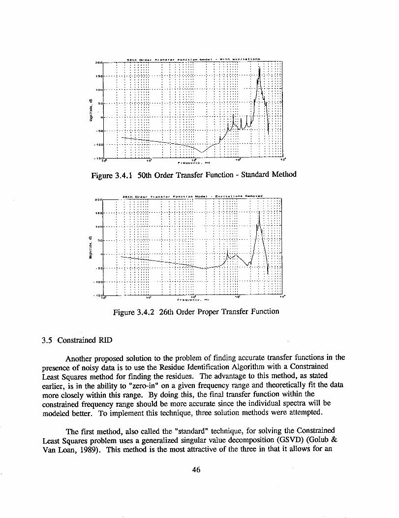
5Otll Order Transfer Punctlon MOdel " W ith e xcitat long

°* iiiiiii iiiii!ili iiiiiiiii iiilil........iii..........................................ii!iiiiiiii!iii!i!!i!i!!ii!iiiii!ii!i!iiii!ii!!i!!iliiiiiii!iiiii!!!i!iiilO( i

=_ 50 ..... '---' .... , -'-'- '-........ : - - -' - -' - : -'-'-'-'-' ..... " - - : - : "" :"-'-:': ..... :" ":" _ ":': !

o

-_5_0 .... :::::1.' ...... ;;'_ " ; ; ;::'",_ _o"Frequency, HZ

Figure 3.4.1 50th Order Transfer Function - Standard Method

2_th Order Transfer Function Model - Sxcltatlons Removed

tO!!!i !-5 ..........

- 15000 to' t1_ '1_ 11_

Frequ*ncv, Hz

Figure 3.4.2 26th Order Proper Transfer Function

3.5 Constrained RID

Another proposed solution to the problem of finding accurate transfer functions in the

presence of noisy data is to use the Residue Identification Algorithm with a Constrained

Least Squares method for finding the residues. The advantage to this method, as stated

earlier, is in the ability to "zero-in" on a given frequency range and theoretically fit the data

more closely within this range. By doing this, the final transfer function within the

constrained frequency range should be more accurate since the individual spectra will be

modeled better. To implement this technique, three solution methods were attempted.

The first method, also called the "standard" technique, for solving the Constrained

Least Squares problem uses a generalized singular value decomposition (GSVD) (Golub &

Van Loan, 1989). This method is the most attractive of the three in that it allows for an

46

analyticalsolution to the problemwhile usingall availabledata. Thus, when it works, the

GSVD solution method provides the best results of the three techniques. The problem with

this method is computer memory. In particular, the GSVD itself requires a great deal of

memory. For example, with the 2,048 frequency point SSME data f'lles, a matrix is

generated in the solution of the GSVD problem that is 4,096 by 4,096 (128Mb, assuming

double precision). Clearly, from a memory standpoint, this presents an insurmountable

problem for most computers. Thus, the following two solution methods are presented as

alternatives to circumvent this problem.

The second method used to solve the Constrained Least Squares problem is to use the

standard GSVD technique but with fewer frequency points. Since the size of the matrices, in

terms of memory required for storage, varies with the square of the number of frequency

points, using fewer points can result in significantly smaller storage requirements. The

obvious problem with this method is that the user is required to make a judgment as to which

frequency points to omit in the modeling process. The omitted points are then not

considered in terms of the Constrained Least Squares solution. At the present time, several

ideas are being considered for selecting the points to omit. These range from omitting every

third frequency point to omitting those points which are "close" to nearby points in terms of

magnitude. However, at this point no method has been found which guarantees satisfactory

results.

The third and final solution method for solving the Constrained Least Squares

problem is to apply an iterative technique. In particular, a sequential quadratic programming

(SQP) method is used to solve the CLS problem, as found in the Matlab ® optimization

toolbox (Grace, 1992). However, this method suffers from the standard shortcomings in

iterative techniques such as convergence problems, local minima, and the need for a "good"

initial guess. In addressing one of these problems, preliminary results show that the standard

least squares solution provides a good starting point for the constrained optimization routine.

Unfortunately, it appears that this method is also limited by the size of the SSME data files.

47

4.0 ENHANCEMENTS TO THE SSME CODE

Several new C main codes have been written to round out the functionality of the

SSME spectrum modeling and transfer function ID code and to ease the transfer of data

between the SSME code and other software programs. The new main programs allow

generation of SISO models from time data without resorting to other software packages, and

SISO transfer function models may be generated as numerator and denominator polynomials,

state-space realizations in observer canonical form (Kailath, 1989, p. 50), or vectors of

transfer function poles and zeros. A listing of the new codes, along with instructions for

their use is presented.

eig.c: Calculate the eigenvalues of a matrix.

usage: eig filein fileout bal/nobal [tsl

f'dein = Name of the file containing the matrix for which the eigenvalues

are to be calculated. The file should be in standard matrix

format (STMF).

fileout = Name of the output file containing the eigenvalues. The file is

four columns in STMF. The first contains the real part of the

eigenvalues; the second is the imaginary part. The third column

is the damping ratios of the eigenvalues and the fourth contains

the eigenvalue resonant frequencies.

bal/nobal = Input argument specifying whether or not balancing is

performed on the input matrix before calculating the

eigenvalues.

ts Optional argument. If the damping ratios and resonant

frequencies are to be calculated for a discrete-time system, ts is

the sampling time (sec). Otherwise, ts may be omitted.

stabsort.c: Given a set of complex z-plane eigenvalues, retain the stable

eigenvalues in an output file.

usage: stabsort filein fileout

filein = Name of the input file containing the eigenvalues to be sorted.The file should be a 2 column matrix in STMF in which the

first column contains the real parts of the eigenvalues and the

second column contains the imaginary parts of the eigenvalues.

48

fileout = Name of the output file into which the stable eigenvalues will bewritten. The f'de will contain a two column matrix in STMF in

which the first column contains the real parts of the eigenvalues

and the second column contains the imaginary parts of the

eigenvalues.

pzdbode.c: Generate SISO frequency response for a discrete-time transfer function

given the numerator roots and denominator roots.

usage: pzdbode numroots denroots ts w greal gimag

numroots = File containing the numerator roots as a 2 column matrix in

STMF with the real parts in the first column and the imaginary

parts in the second column.

denroots = File containing the denominator roots as a 2 column matrix in

STMF with the real parts in the first column and the imaginary

parts in the second column.

ts Real value which is the sample period of the system (see).

W Input file in STMF containing a column vector of the frequency

points (rad/sec) at which the transfer function response is to beevaluated.

greal = Name of the file in which the real part of the frequency

response is stored as a column vector in STMF.

gimag = Name of the file in which the imaginary part of the frequency

response is stored as a column vector in STMF.

r2poly, c. Given a set of polynomial roots, generate the polynomial.

usage: r2poly filein fileout

filein = Name of the input f'de containing the polynomial roots. The file

should be a 2 column matrix in STMF in which the first column

contains the real parts of the roots and the second column

contains the imaginary parts of the roots.

fileout = Name of the output file into which the polynomial coefficientswill be written. The file will contain a two column matrix in

49

STMF in which the first columncontainsthe real partsof thecoefficientsandthe secondcolumn containsthe imaginarypartsof the coefficients.

O°2SS. C•. Generate a SISO state-space realization in observer canonical form

(Kailath, 1989, p. 50) given transfer function numerator and

denominator polynomials.

usage: O_2ss numpoly denpoly A B C D

numpoly = Input f'de containing the numerator polynomial coefficientsstored as a column vector in STMF. If there are n coefficients,

the first multiplies z to the (n-1)st power and the last multiplies

z to the 0 power. The coefficients must be real numbers.

denpoly = Input file containing the denominator polynomial coefficientsstored in the same format as that used for the numerator

coefficients file.

A,B,C,D = Names of the corresponding output files into which the

appropriate state-space realization matrices will be written inSTMF.

stmf2mat, c: Given an input file in STMF, create an output file that is identical to

the input file except that the first line containing the matrix dimensions

has been omitted. The results in an ASCII file that may easily be

imported to Matlab ® or other software packages.

usage: stmf2mat filein fileout

filein = Name of the file containing the input file in STMF.

fileout = Name of the file which will contain the output ASCII file in the

format described above.

These new codes add functionality, power, and utility to the SSME spectrum

modeling and transfer function ID code and make it easier to interface between this code and

other software products.

50

5.0 ENHANCEMENTS TO XPLOT

Several new features have been added to the XPLOT graphics package developed at

Ohio University. These features are intended to make the program more user friendly and

practical in terms of working with the SSME data. In addition, other improvements are

suggested to broaden the range of XPLOT's capabilities. These are summarized in Section

5.2.

5.1 Additional Features

One feature which has been added to XPLOT is the ability to generate linear,

semilog, loglog, and polar plots. These four plot types will allow the user to view SSME

data (or any data set in STMF) in any 2-D format desired. To select a plot type, the user

simply clicks on the button labeled "plot type u and selects linear, semilogx, semilogy,

loglog, or polar from the menu. To switch plot formats, the process is repeated. This easy

switching allows the user to quickly view multiple plot formats to determine the best one for

viewing the current data set(s).

A second feature added to XPLOT is a grid display option for each of the four

previously mentioned plot types. This option puts an appropriate grid on the current plot

type being used. To implement this new feature, the user simply clicks on the "grid-on"

button to add a grid or clicks on the "grid-off" button to remove the grid. Note that the

"grid-on" and "gfid-off" buttons are the same button but only one is active at a given time.

A third and final feature added to XPLOT is the ability to fix the cursor to a data set.

This is done by clicking on the graphics window twice. At this point, the cursor is fixed to

the data set and the current data point value, in x and y coordinates, is displayed in the upper

fight-hand corner of the graphics window. To move the cursor along the data, the left and

fight arrow keys should be used. To exit this mode, simply click on the "x, y position"

button. Note that full instructions for this feature are presented on the screen by clicking on

the "x, y position" button before fixing the cursor to the data.

5.2 Possible Future Additions

One possible addition for XPLOT is a 3-D plotting capability. Adding this feature

depends on whether this is possible using X-Windows. One reason for adding this feature is

the desire to view modes as they shift in frequency with time; for example, when the rotor is

being run up to speed.

Another future addition is to add the ability to store the cursor display in a disk file

upon pressing a mouse button. This feature would work in conjunction with fixing the

cursor to a data set. One reason for adding this feature is to allow the user to select points

which he believes are modes and save those points in a file for future analysis.

51

6.0 CONCLUSIONS

This chapter summarizes the results presented in this report and details work which

has yet to be completed. Section 6.1 explains Ohio University's attempts to apply the SSMEtransfer function modeling code to SSME data. Also included in Section 6.1 is a brief

overview of enhancements to the SSME code and XPLOT. Section 6.2 details plans for

future work on the project.

6.1 Observations and Summary Results

This report demonstrates that a straightforward application of the code results in

transfer functions which are not realistic in that they contain a huge hump in the magnitude

spectrum at frequencies higher that the quarter sampling rate of 2,560 hertz. One possible

explanation for this phenomenon is that the modeling technique results in multiple lightly

damped poles in the frequency range spanning the hump while giving far fewer lightly

damped zeros to cancel the poles' effects. Several attempts were made to alleviate this

problem as explained below.

One attempt at generating better transfer function models involves the so-called

trending method. This method involves first extracted a general trend from the data, thus

flattening the spectrum. The flattened spectrum and the trend are then modeled separately.

These two models are then combined in series resulting in a model of the actual spectrum.

The advantage to this technique is that the trend requires only a low order model while the

model of the spectrum should have more uniform spacing of poles since the spectrum is

relatively flat. As shown in the report, the technique does indeed reduce the hump in the

transfer function. However, it has not at present been verified if the resulting transfer

function is an improvement over that obtained by the direct method.

Rather than trying to reduce the hump, an attempt was made to simply filter the initial

time data with a low-pass filter with cutoff frequency fs/4. This filtering resulted in the data

being severely attenuated at the frequencies where the hump would normally occur. It was

hoped that this process would result in a better transfer function model at frequencies below

the quarter sampling frequency since more model order would be used in this area.

However, as shown in Section 3.3, the end result was a negligible change in the transfer

function for these frequencies. Thus, filtering the data failed to give improvement in the

resulting transfer function.

Another attempt to reduce the hump in the transfer function involved eliminating the

excitations from the transfer function. As shown in the theory, the proper transfer function

has the poles corresponding to excitations removed. It was hoped that eliminating the

excitations before the modeling process would result in better pole/zero spacing, thus

reducing the hump. However, as shown in the report, the effect of removing the excitations

was negligible in terms of the hump in the transfer function. It is therefore concluded that

failing to eliminate the excitation poles from the transfer function does not cause the hump.

52

A final attempt at improving the final transfer function involved applying the Residue

Identification Algorithm with Constrained Least Squares. Theoretically, this technique will

allow for a tighter fit of the data within given frequency ranges, thus giving more accurate

transfer functions within those ranges. Unfortunately, the size of the SSME data files results

in large memory requirements which cannot currently be overcome using the standard

solution method for CLS. Thus, two other options were presented but both had serious

limitations. The end result is that CLS has not been fully applied to this problem.

In addition to the above work, several enhancements to the SSME code and the

graphics package XPLOT have been completed. The enhancements in the SSME code allow

the user to fully implement the SSME transfer function modeling code without going to an

outside software package such as Matlab ®. Also, the improvements in the XPLOT packageallow the user to better examine the data in terms of the format of the plots and reading the

data values from the graph.

6.2 Future Work

Several areas are proposed for future work on the SSME project. These areas are

listed below with a short explanation of each.

1. Obtain Direction On Software Platform And XPLOT.

The current code being used to implement the SSME transfer function

modeling algorithm is believed to be self-contained. However, if XPLOT

continues to be used, future work is necessary as detailed in this report. Also,

there has been discussion of reverting to Matlab ® rather than using the SSME

code. If this is implemented, it will be necessary to test the original m-filesand deliver these files to NASA MSFC.

. Evaluate Modeling Effectiveness By Comparing To MARSYS Or Other

Results

Currently, Ohio University has no transfer function models for the SSME with

which to compare the results obtained from the SSME transfer function

modeling code. In order to evaluate the output of the code, it is necessary to

have a reference transfer function (or at least an approximation of the transfer

function).

3. Investigate Numerical Approaches To Constrained RID

As mentioned earlier, the analytical solution of the Constrained RID problem

is currently not feasible due to memory constraints on Ohio University's and

NASA MSFC's computers. To circumvent this problem, numerical

approaches have been explored to some extent. However, further investigation

53

.

.

is necessary to determine if numerical approaches will work.

Add Ability To Use ERA Given Input And Output Time Sequences

Currently, ERA can be used to obtain a model if an input sequence

representing the system pulse response is given. However, it would also be

desirable to have a version of ERA which produces a model given the input

and output responses of the system. This ability can be added to the currentversion of ERA.

Investigate Effectiveness Of TLS

Another approach which may prove useful is to apply the Total Least Squares

algorithm to RID. This technique is discussed fully in Section 2.4.3.

However, at the present time, no work has been completed involving applying

to SSME data.

54

7.0 REFERENCES

Bartholomew, D. L. (1992), "Spectral Modeling of the SSME: Enhancements and a

Software System," Master of Science Thesis, Ohio University, August, 1992.

Bendat, J. S. and A. G. Piersol (1980), Engineering Applications of Correlation and Spectral

Analysis, John Wiley and Sons, New York.

Cooper, G. R. and C. D. McGillem (1971), Pr0babilistic Methods of Signal and System

Analysis, Holt, Rinehart, and Winston, Inc., Fort Worth, Texas.

Golub, G. H. and C. F. Van Loan (1989), Matrix Computations, Second Edition, The Johns

Hopkins University Press, Baltimore.

Grace, A. (1992), Optimization Toolbox User's Guide, The Mathworks, Inc., Natick, MA.

Irwin, R. D. (1990), "System Identification and Controller Design Using Experimental

Frequency Response Data", Final Presentation Materials, 1990 NASA/ASEE Summer

Faculty Fellowship Program, Marshall Space Flight Center, Alabama, August, 1990.

Irwin, R. D., Mitchell, J. R., Brown, J., Bartholomew, D., and Medina, E. (1992),

"Advances and Applications of Transfer Function Modeling Techniques to the Space Shuttle

Main Engine", Final Report, NASA Grant NAG8-167, NASA George C. Marshall Space

Flight Center, Alabama 35812.

Juang, J-N. and R. S. Pappa (1985), "An Eigensystem Realization Algorithm for Modal

Parameter Identification and Model Reduction", AIAA Journal of Guidance and Control,

Vol. 8, No. 5, pp.620-627, Sept-Oct 1985.

Juang, J-N. and R. S. Pappa (1986), "Effect of Noise on Modal Parameters Identified by the

Eigensystem Realization Algorithm", AIAA Journal of Guidance and Control, Vol. 9, No. 3,

pp. 294-303, May-June 1986.

Kailath, T. (1989), Linear Systems, Prentice-Hall, Inc. Englewood Cliffs, New Jersey.

Longman, R. W. and J-N Juang (1989), "Recursive Form of the Eigensystem Realization

Algorithm for System Identification", AIAA Journal of Guidance and Control, Vol. 12, No.

5, pp. 647-652, Sept.-Oct. 1989.

Medina B., E. A. (1991), "Multi-input, Multi-output System Identification for Frequency

Response Samples with Applications to the Modeling of Large Space Structures", M.S.

Thesis, Ohio University, November 1991.

55

Phillips, C. L. and H. T. NagleJr. (1984),Digital Control System Analysis and Design,

Prentice-Hall, Inc., Englewood Cliffs, New Jersey.

Phillips, C. L. and H. T. Nagle Jr. (1990), Digital Control System Analysis and Design,

Prentice-Hall, Inc., Englewood Cliffs, New Jersey.

Van Huffel, C. and J. VandewaUe (1991), The Total Least Squares Problem: Computational

Aspects and Analysis, Society for Industrial and Applied Mathematics, Philadelphia, Pa.

56