N94-14644

A Rational Interpolation Method to Compute

Frequency Response *

Charles Kenney, Stephen Stubberud, and Alan J. Laub

Department of Electrical and Computer Engineering

University of California

Santa Barbara, CA 93106-9560

Abstract

A rational interpolation method for approximating a frequency response is presented.

The method is based on a product formulation of finite differences, thereby avoiding the

numerical problems incurred by near-equal-valued subtraction. Also, resonant pole andzero cancellation schemes are developed that increase the accuracy and efficiency of the

interpolation method. Selection techniques of interpolation points are also discussed.

1 Introduction

Consider the linear time-invariant system given by the state-space model

= Az + Bu (1)

y = c= (2)

where A E _t_ rSAX_tA , B E _ ytAXytB, C E _tftCXnA, and the state vector, input vector, and

output vector, =, u, and y, respectively, axe properly dimensioned. We shall refer to the

matrices, A, B, and C, as the state coupling matrix, the input coupling matrix, and the

output coupling matrix, respectively.

The frequency response of such a modeled system is defined as the Laplace transform of

the input-output relationship evaluated along the jw-axis,

G(,,,)= c(j,,,z- A)-IB (3)

where

0<w<oo.

*This research was supported in part by the Air Force Office of Scientific Research under Contract No.AFOSRgl-0240.

PRE-,-'_"EiZ)tNGPAQE BLANK NOT FN.MED

413

https://ntrs.nasa.gov/search.jsp?R=19940010171 2019-02-03T11:38:35+00:00Z

In this paper, a fast and reliable interpolation method to compute frequency response is

presented. The basic idea of this method is based on the simple Taylor series approximation

G(w + h) = To + Tab +... + Tkhk+ Ek (4)

but considered in the general interpolation form with k + 1 interpolation points ho, hi, • •., hk:

G(w+h)=Go+Gl(h-ho)+...+Gk(h-ho)(h-hl)...(h-hk-1)+ Ek. (5)

The coefficient matrices, Go, G1,..., Gk are of size nc x nB as is the truncation error Ek.

Therefore, the cost of evaluating the matrix polynomial approximation

P_(h)=Go+Gl(h-ho)+...+Gk(h-ho)(n-hl)...(n-hk-1) (6)

is just knB nc floating-point operations (flops). The cost of computing each coefficient ma-

trix is approximately the same as evaluating G by the method that would normally be

preferred.

The polynomial interpolation scheme works well as long as _ is not near a resonant pole or

zero of the system. In order to avoid this problem, we introduce methods of preliminary

pole and zero cancellation. These greatly increase the accuracy of the interpolation scheme

while causing only a negligible increase in the cost of computing the coefficient matrices.

We shall also discuss the implementation of this algorithm including ideas on the selection

of interpolation points.

2 Existing Frequency Response Methods

2.1 Straightforward Computation

An obvious method for computing frequency response for a system modeled in state-space

form is first to perform an LU decomposition in order to solve the linear system

(j_I- A)X = B,

followed by a matrix multiplication involving the solution to (7),

(T)

G(_) = ca.

This method does not exploit any special structure, e.g., sparse or banded, and therefore

would only be used for general systems. To compute a frequency response implementing

this method, for just one value of w, approximately "_nA13 q. 1(7l B Jr nc)n2A "b nAnBRC flopsare required. As the number of desired frequency points becomes large, the calculation of

the entire frequency response becomes computationaUy intensive.

414

2.2 The Principal Vector Algorithm

In order to reduce computation cost, several methods have been developed in order to re-

duce the cost of solving the linear system (?) either by exploiting the structure of the state

coupling matrix or by implementing a similarity transformation to put the matrix A into

an exploitable form. One method of the latter variety is the Principal Vector Algorithm

(PVA) [10].

The idea of the PVA is to initially transform the state coupling matrix into a Jordan

Canonical Form (JCF). The algorithm uses the principal vectors to compute the JCF in a

more accurate way than previous such algorithms. Let

A = M-1JM (8)

where J is in Jordan form. If we substitute this identity into (3), the frequency response

becomes

G(w) = CMM-I(jwI- A)-IMM-1B

= 6_(jwi_ j)-l:_. (9)

The initial transformation using the PVA to compute the JCF requires only O(n3A) flops if

the state coupling matrix is not defective while O(n4A) flops axe required if the matrix A

is defective. Note that this transformation only occurs once, thus the cost is only incurred

once. The a_lwntage occurs in computations at each frequency point where the cost is

reduced to O(nA + nAnBnc) flops in the nondefective case and O(]na + nAnBnc) flopsin the defective case. So the computational saving occurs after the computation of one

frequency point in the former case and nA frequency points in the latter case.

Although this algorithm produces significant savings in the computational cost of a fre-

quency response, it can also frequently encounter numerical instabilities. First, the JCF is

extremely unstable. The slightest perturbation can change a defective matrix into a non-

defective matrix. Another problem is that the similarity transform may be ill-conditioned

with respect to inversion depending on the basis of eigenvectors. If they axe guaranteed

to form a matrix which is wen-conditioned with respect to inversion as would occur if the

matrix were normal, the algorithm is very effective.

2.3 The Hessenberg Method

Another algorithm which uses similarity transformations to put the state coupling ma-

trix into an exploitable form is the Hessenberg Method [4]. This algorithm is the current

standard for computing the frequency response for generic dense systems. The Hessenberg

Method, as its name implies, performs an initial transformation on the state coupling matrix

to reduce it to upper Hessenberg form. So in this case, we use the identity

A = 0-1HQ,

415

whereH is in upper Hessenberg form, instead of the JCF identity (8), in the frequency

response (3).

As with PVA, this initial transformation is performed only once at the start of the algo-

rithm at a cost of O(n_) flops. When this transformation is used, the cost of computing

the frequency response at each value of w becomes O(n2A(nS + 1)+ nA nBnc) flops. Usually,

nB _. nA so a significant reduction in computation can be realized.

Fortunately, there always exists an orthogonal transformation to reduce the state coupling

matrix into an upper Hessenberg form. This prevents W-conditioning from being introduced

into the calculations by the similarity transformation as can occur with the Principal Vector

Algorithm.

2.4 Sparse Systems

Many of today's large ordered systems are sparse systems. A sparse system is one whose

modeling matrices have relatively few nonzero entries when compared to the total numberof entries. In such cases the Hessenberg Method should not be used. Instead of maintaining

sparsity, the initial transformation will create a large dense system which then must be

solved. There exist many storage techniques for sparse matrices which require a significantly

smaller amount of memory allocation than a full matrix of the same order would require.

Also, sparse matrix algorithms have been developed to exploit sparsity in order to reduce

the computational costs in comparison to their dense counterparts. (See [6], [9], and [7].)

These algorithms attempt to prevent the cost of solving the linear system (7) from growing

to O(n_) flops.

2.5 Frequency Selection Routines

The cost of computing an entire frequency response can also be reduced by eliminatingneedless recalculations or overcalculations in attempts to get a desired resolution in the

solution. When the frequency mesh is too coarse to give the required information, usually

the user recomputes the entire frequency response. Often, the response from the previously

computed frequency values either is recalculated or just ignored in the new calculation.

Also, many times the user creates a fine frequency point mesh across the entire frequency

range. Usually, only in small subregions is the finer mesh needed. A coarser mesh would

suffice over the rest of the frequency range.

In an effort to eliminate these unnecessary calculations but still give the required accuracy,

so-called adaptive routines have been developed. These routines adapt the frequency point's

selection to the characteristics of the system being analyzed.

One such adaptive scheme is similar in nature to the QUANC8 adaptive integration routine

[1]. The basic idea is first to select the endpoints of an interval in the desired frequency

416

region. Then the frequency responses of the two points are compared. If the difference

between their magnitudes or their phases is greater than specified tolerances, the interval

is divided in half. Then the three points are compared. If their differences are outside

the tolerances, the subintervals are again halved. This subinterval halving continues untilthe tolerances are met across the entire interval or until a specified number of frequency

points has been calculated. A single-input single-output variation of a method based on

subinterval halving has been implemented commerdaUy [5].

The use of a priori information, e.g., the locations of poles and zeros of a system, can also

be used in the choice of frequency locations. More points are placed in the areas where the

poles and zeros of a given system have an effect. Fewer points are placed outside these areas.

Such a method is now being implemented in a linear system package [2] to automatically

choose the frequency range over which the frequency response is computed as well as to

determine the number of points needed to be calculated.

These adaptive schemes also can be combined to form hybrid routines. This would permit

an initial placement of points with the a priori method and then create the frequency mesh

to join the regions between the areas of the initial placement.

3 Polynomial Interpolation

In order to compute the coefficient matrices, G1,..., Gk, of the interpolation equation

Pk(h) = Co + Gl(h - h0) +... + Gk(h - h0)(h - hi)...(h - hk-1) (10)

finite differences win be employed. The first-order difference is defined as

M[ho,hd- M(hx)- M(ho) (11)hi - ho

while higher-order differences are defined as

M[ho, hl,...,h,_] = M[hl,...,h_]- M[ho,...,h,,-1] (12)h, - ho

Ifwe let

where

M(h) - (jhI- Ao) -1

Ao = -jwI + A,

the kth-order interpolation approximation can be written as

Pk(h) = C(M(ho) + M[ho, hl](h- ho) +...

+ M[ho, hl, ..., hk]( h - ho)( h - hi)...(h - hk-1) )B

(13)

(14)

(15)

417

with the interpolation error

Ek

Now, for convenience, define

P_(h)

= + h)- Pk(h)k

= C(M[ho, hl,...,hk, h] H(h- hi))B.iffi0

= M(ho) + M[ho, hl](h- ho) +...

+M[ho, hl,...,hk](h - ho)(h - hi)" .(h - hk-1)

(18)

(17)

and

Ek = M(h)- Pk(h)k

= MIho, hl,...,hk, h] I_(h- h,). (18)iffi0

Although finite differences have a certain elegance to their formulation, they can encounternumerical inaccuracies due to the subtraction of neax-equal-vaiued quantities. An extreme

example of this is the case in which all of the interpolation points axe the same. In theory,the first-order difference is exactly the first derivative of M, but numerically it is useless.

Fortunately, the differences of the resolvent function (13), can be expressed in matrix prod-

uct forms which avoid these cancellation problems as the following theorem shows.

Theorem 1 For the resolvent function, the matriz difference functions in (12) satisfy

M[ho, hl,...,h,,_] = (-j)'_M(ho)M(hl)...M(h,,_). (19)

Preo_. Using (13)

M(hl) - M(ho) = (jhlI- Ao) -1 - (jhoI- Ao) -1

= (jhoI - Ao) -1 {jhoI - ,4o - (jhlI - Ao)) (jhxI - Ao) -1

= (-j)(h_ - ho)M(ho)M(h_).

Thus the first finite difference becomes

M[ho, hl] = -jM(ho)M(hl)

which proves (19) for m = 1. Now suppose that (19) is true for m-1. Since M(ho)'..., M(h,,,)

all commute with each other, we find that

M[h0, hi,..., h,n]

418

= (M[hl,...,hm]- M[ho,...,hm-1])/(hm- ho)

= (-j)m-l(M(hl)...M(h,,_)- M(ho)'"M(hm-1))/(hm-ho)

= (-j)'n-l(M(hl)...M(h,n_1))(M(h,_)- M(ho))/(hm-ho)

= (-j)'n(M(hl)...M(h,n_l))M(ho)M(h,,_)

= (-j)n_M(ho)M(hl)...M(hm).

Thus (19) is true for m and thus, by induction, the theorem is true. 13

If we now substitute the resolvent identity (19) into (17) and (18) and use the commutative

property of the resolvent functions, the interpolation approximation becomes

f:'k(h) = M(ho) + (-j)M(hl)M(ho)(h - ho) +...

+(_j)kM(hk)M(hk_l)...M(ho)(h - ho)...(h - hk_l) (20)

with the error formula

_k = M(h)- Pk(h)k k

= (_j)k+1 I"IM(hi) 1"_(h- hi)M(h). (21)i--O i=O

The next lemma gives an interpolationseriesfor the resolventusing the originalk + 1

interpolationpointsand settingallof the higher-orderinterpolationpointsequal to zero.

For conveniencewe shalluse the notationM(0) = Mo. Note that ifallofthe interpolation

pointsare setequal to zerothe analysiswould be thatof the Taylorseries.

Lemma 2 Let ho,..., hk be given and set hm = 0 for all m > k. For

Ihl< min ]j_-A 1, (22)_e^(A)

M may be ezpanded as

+oo m m-1

M(h)= _ (-#)" ]-[M(_) ]'I (h- h,).m=O i=0 i=0

Proo_ Let l > k. By (21),

l m m-1

M(h)- _ (-j)_ l'I M(h,)II (h- h,)m=O i=0 i=O

l t

(_j)_+l_ M(h,)l-I(h- hi)M(h)i=O i--O

k k t

= (_j)t+,I"[M(h,)I'[(h-h,)t_(h)I-IMohi=0 i--O i=k+l

= (_j)t+l M(hi) II(h- hi)M(h) (hMo) t-k.

(23)

419

But (hMo) t-k --* 0 as t --, +oo if and only if p(hMo) < 1, which is the well-known

convergencerequirementfora geometricseries.From the definitionof M0, we have 34"o=

(j_I- A) -I. Hence,

p(jhMo) = Ihl/ rain IJ - l_eA(A)

-lhl/,•

where

r = min Ij_--A[. (24)_e^(A)

D

This lemma isalsoimportant in the development of a pole and zerocancellingroutine.

4 Pole and Zero Cancellation

Polynomial interpolation approximation works well unless the LTI system being analyzed

has poles or zeros near the imaginary axis. Such poles and zeros axe called resonant poles

and resonant zeros. The following examples provide the general idea of the effect.

Example: The deleterious effect of poles and zeros can be illustrated by means of a scalar

rational function example. Consider

f(x) = 1-{- 2z + 3z 2 = 1+ 3z + 6z 2 +... (25)l-z

We can use a polynomial approximation to evaluate this function at various values of x.

Suppose that we choose a second-order polynomial approximation:

/(x) = 1 + 3z + 6x 2.

Ifwe evaluatef forz - 0.01and x = 0.99,we get the approximations

/(0.01) = 1.0306,

and

/(0.99) = 9.8506,

respectively. If we compare these to the actual values,

f(0.01) = 1.0306061

and

f(0.99)- 592.03,

420

we can see that as we approach a pole, a much higher-order approximation is required in

order to get even modest accuracy.

However, ifinitiallywe eliminatethe polebeforewe make our calculationsfor valuesnear

z = 1, the accuracy of the method increasesdramatically. Again, use a second-order

approximation with pole cancellation,and we get

i(x)=(1-x)1+2z+Sx _ =(1+2_+3z2).1-z

After evaluating], we let

/= ](1- z)'

As can be seenin thiscase,the second-orderinterpolationisexact.In most cases,however,

only a marked increasein accuracyisrealized.

In order to cancela polein our frequencyresponse,we write

(jh + j_ - A)/(h)

M(h) = (jh + j_- A)

and then finda polynomial approximationof(jh+jw-A)M(h). Therefore,our interpolation

becomes

G(w + h) = Go+ Gl(h - ho) +'" + Gk(h - ho) " "(h - h_-l) (26)(jh + j_ - _)

where the coefficient matrices are for a system devoid of the resonance problem. The

following lemma shows how to compute the new coefficient matrices while preserving the

form of the interpolating series.

Lemma 3 Let ho,..., hk be given and set hm = 0 for all m > k. For [hI < r, where r is

defined in (e4), define the eoe._cient matrices F(mn) implicitly via

n +co m-1

I_(Jh + jw - At)M(h) = __, F_n) YI (h- hi) (27)£----I m=O i=0

Then

and

F_ ) = (-J)'_l'iM(hi) ,i=O

(28)

r_") = (jh_ + j_- _.)r_ _-') + j_£_-_), re=o,1,... (29)

where we define F{__ = 0 .for all t.

421

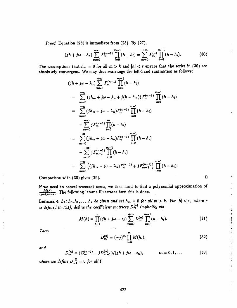
Proof. Equation (28) is immediate from (23). By (27),

4-oo m-1 -I-oo m-1

(_'h+_ - _.)E: F_"-11I] (h- h,)= _ r_")II (h- h,). (30)m=0 i----O m=O i--O

The assumptions that hm = 0 for all m > k and Ihl < r ensure that the series in (30) are

absolutely convergent. We may thus rearrange the left-hand summation a_ follows:

-I-oo m-1

(_h+ _ - _.1E: F_"-1_I] (h- _1m---0 i------O

-Foo m-1

= _,(jh_+j_-_.+j(h-h_)lr(Z -1) _I(h-h,)m=O i---0

-I-oo m-1

= _ (jh_+_- _.)F_"-1)II (h- hi)m-----O i=0

q-oo rn

+ _ jF_"-I_H(h - hi)m--0 i--0

+oo m-1

= _ (ih_+_- _.)r_"-_11-I(h- h,)m---O i----O

+oo ,_r("-1) m-1+ ;E J-_-1 II (h- hi)m--0 i----0

+oo m-1

= _ ((jh_+i_- _.)r_"-' +jr_"._-:_)II (h- hi)m=O i----O

Comparison with (30) gives (29). O

If we need to cancel resonant zeros, we then need to find a polynomial approximation of

MIh) The following lemma illustrates how this is done.(jh+_-,)"

Lemma 4 Let ho, hl,...,hk be given and seth,,= O for all m > k. For Ihl < r, where r

is defined in (24), define the coefficient matrices D_ '_) implicitly via

n +oo m-1

M(h) = I_(Jh + iv- zt) _ D (n) H (h - hi). (31)t=l m-----O i=0

Then

and

D_ ) =(-j)mHM(hi),i--0

D (_) = (D ("-1) - jD(")l)/(jh + jw I Z_),

where we define D (t) = 0 for all L-1

(32)

m=0,1,... (33)

422

Proof. The proof is similar to that of the preceding lemma except that we start with

the identity

+oo m-1 +co m-1

(jh + j_,- _.1_ Dk"_II (h- h,) = _ Dk"-' II (h- h,)m=O i=0 m=O iffiO

and continue from there.

(34)

D

5 Frequency Response Interpolation Algorithm

Step 1 Solve for X0 in

(j(ho + _)I- a)Xo = B ,

and then solve recursively for Xa,..., Xk in

(j(h,. +,_)x- A)X,. = -jx,___

(35)

(36)

Step 2 Let X_ ) = X,n and define

x_ = (j_. + j,,- _t)x_ -_)T_-_..,,__Y(t-_)

with Xtl = 0 for 0 _<t <_ n.

Step 3 Let X(_")(°) = X(_") and define

x_.)(o = (x_.)(t-,)- 3x(..")_(,t))/(_h.,+ _,, - _) ,

with Xt_l - 0 for 0 _ t _< I.

Step 4 Form the coefficient matrices Go,...,Gk via

G = CX_")(O .

, o _<m < k, (37)

0 < m _< k, (38)

(39)

Step 5

G(_+ h) = (Go + G,(h- ho) +...+ Gk(h- ho)...(h- h(k-1)))l

rii=,(jw + jh - zi)

I'[n_fl(jw + jh - A._)(40)

Remark

The method used to solve the recursive linear systems in the first step of the algorithm

depends on the initial structure of the LTI system being investigated. If the system has an

exploitable structure such as sparsity, an algorithm that exploits that particular structure

will be used. If no such structure exists, an initial similarity transformation, most likely to

upper Hessenberg form, will be applied to the system.

423

6 Interpolation Point Selection

The placement of the interpolation points is of great importance in getting a good ap-

proximation to the frequency response. We have tested three simple methods to place the

interpolation points: linear, loglinear, and Chebyshev. We have also tested placement using

the a priori information of the pole locations.

Sincefrequencyresponseisusuallyplottedagainstfrequencyon a log scale,the use oflin-

earlyspaced interpolationpointsdoes not usuallyperform well.Itplacestoo many points

at the end of an interval.Both the loglinearand the Chebyshev interpolationpoint place-

ments have shown promise. The loglinearplacement techniqueusuallygivesan excellent

approximation in the beginningto the middle of an interval,but sometimes can failmis-

erablyat the end of an interval.The Chebyshev interpolationpoints(see[8])spread the

approximation errorfairlyevenlyacrossthe interval.However, severaltimes the errorof

the Chebychev selection,although acceptable,islargerthan that of the acceptablerange

ofa loglinearinterpolationofthe same size.Currently,we areinvestigatingpossiblehybrid

techniquesto exploitthe best ofboth placement schemes.

In the caseswhere we have triedplacinginterpolationpointswith the knowledge ofthe poles

and zerosof the system the resultshave been mixed in comparison to the two previously

mentioned techniques.What has been learnedisthat under no circumstancesshould the

interpolationpointsbe the same as the resonantfrequencyofa resonantpoleor zero.How-

ever,placingan interpolationpointnearthe resonantfrequencyimproves the approximation

significantly.

7 Conclusion

In this paper we have presented a rational interpolation method for computing the frequency

response of a system. A significant computational savings can be achieved over several ofthe current methods for computing a frequency response. An error analysis for the method,

together with other details, can be found in [3].

The method presentedin thispaper avoidsthe numericalproblem of subtractionof near

equal quantitiesin the differenceterms by usingthe resolventidentityof Theorem i.Also,

simplepoleand zerocancellationtechniquessignificantlyincreasethe accuracy of the algo-

rithm.

We are currently writing a software package to implement the algorithm in this paper. In

addition, we are extending this algorithm for use with descriptor systems.

424

References

[1] Forsythe, G.E., M.A. Malcolm, and C.B. Moler, Computer Methods for Mathematical

Computations, Prentice-Ha/l, Englewood Cliffs, N J, 1977.

[2] Grace, A., A.J. Laub, J.N. Little, and C. Thompson, Control System Toolboz, User's

Guide, The MathWorks, Natick, MA, Oct. 1990.

[3] Kenney, C.S, S.C. Stubberud, and A.J. Laub, "Frequency Response Computation ViaRational Interpolation," Proceedings of the I 99_ IEEE Symposium on Computer-Aided

Control System Design, pp. 188-195, Naps, Ca/if, March 1992, IEEE Control Systems

Society.

[4] Laub, A.J., "Eilicient Multiwriable Frequency Response Computations," IEEE Trans.

Auto. Control, AC-26 (1981), pp. 407-408.

[5] Lee, E.A., Control Analysis Program .for Linear Systems for MS-DOS Personal Com-puters, User Manuals, CAPLIN Software, Redondo Beach, Calif., April 1990.

[6] Meier, W.A., "Sparse Matrix Applications in Computer-Aided Control System De-

sign," Proceedings of the 199Y, IEEE Symposium on Computer-Aided Control System

Design, pp. 196-203, Naps, Ca/if, March 1992, IEEE Control Systems Society.

[7] Osterby, O. and Z. Zlatev, Direct Methods for Sparse Matrices, Springer-Verlag, Berlin,

1983.

[8]Rivlin,T.J, The Chebyshev Polynomials,John Wiley and Sons,New York, 1974.

[9]Schendel,U., SparseMatrices:Numerical AspectswithApplicationsfor Scientistsand

Engineers,EllisHorwood, Chichester,1989.

[10]Walker, R.A., Computing the Jordan Form for Controlof Dynamic Systems, PhD

thesis,StanfordUniversity,Department ofAeronauticsand Astronautics,March 1981.

425