n+3 aircraft concept designs and trade studies, final report · 2013-04-10 · n+3 aircraft concept...
TRANSCRIPT

E.M. Greitzer, P.A. Bonnefoy, E. de la Rosa Blanco, C.S. Dorbian, M. Drela,D.K. Hall, R.J. Hansman, J.I. Hileman, R.H. Liebeck, J. Lovegren, P. Mody,J.A. Pertuze, S. Sato, Z.S. Spakovszky, and C.S. TanMassachusetts Institute of Technology, Cambridge, Massachusetts
J.S. Hollman, J.E. Duda, N. Fitzgerald, J. Houghton, J.L. Kerrebrock, G.F. Kiwada, D. Kordonowy, J.C. Parrish, J. Tylko, and E.A. WenAurora Flight Sciences, Cambridge, Massachusetts
W.K. LordPratt & Whitney, East Hartford, Connecticut
N+3 Aircraft Concept Designs and Trade Studies, Final ReportVolume 2: Appendices—Design Methodologies for Aerodynamics, Structures, Weight, and Thermodynamic Cycles
NASA/CR—2010-216794/VOL2
December 2010
https://ntrs.nasa.gov/search.jsp?R=20100042398 2020-02-29T02:20:18+00:00Z

NASA STI Program . . . in Profi le
Since its founding, NASA has been dedicated to the advancement of aeronautics and space science. The NASA Scientifi c and Technical Information (STI) program plays a key part in helping NASA maintain this important role.
The NASA STI Program operates under the auspices of the Agency Chief Information Offi cer. It collects, organizes, provides for archiving, and disseminates NASA’s STI. The NASA STI program provides access to the NASA Aeronautics and Space Database and its public interface, the NASA Technical Reports Server, thus providing one of the largest collections of aeronautical and space science STI in the world. Results are published in both non-NASA channels and by NASA in the NASA STI Report Series, which includes the following report types: • TECHNICAL PUBLICATION. Reports of
completed research or a major signifi cant phase of research that present the results of NASA programs and include extensive data or theoretical analysis. Includes compilations of signifi cant scientifi c and technical data and information deemed to be of continuing reference value. NASA counterpart of peer-reviewed formal professional papers but has less stringent limitations on manuscript length and extent of graphic presentations.
• TECHNICAL MEMORANDUM. Scientifi c
and technical fi ndings that are preliminary or of specialized interest, e.g., quick release reports, working papers, and bibliographies that contain minimal annotation. Does not contain extensive analysis.
• CONTRACTOR REPORT. Scientifi c and
technical fi ndings by NASA-sponsored contractors and grantees.
• CONFERENCE PUBLICATION. Collected papers from scientifi c and technical conferences, symposia, seminars, or other meetings sponsored or cosponsored by NASA.
• SPECIAL PUBLICATION. Scientifi c,
technical, or historical information from NASA programs, projects, and missions, often concerned with subjects having substantial public interest.
• TECHNICAL TRANSLATION. English-
language translations of foreign scientifi c and technical material pertinent to NASA’s mission.
Specialized services also include creating custom thesauri, building customized databases, organizing and publishing research results.
For more information about the NASA STI program, see the following:
• Access the NASA STI program home page at http://www.sti.nasa.gov
• E-mail your question via the Internet to help@
sti.nasa.gov • Fax your question to the NASA STI Help Desk
at 443–757–5803 • Telephone the NASA STI Help Desk at 443–757–5802 • Write to:
NASA Center for AeroSpace Information (CASI) 7115 Standard Drive Hanover, MD 21076–1320

E.M. Greitzer, P.A. Bonnefoy, E. de la Rosa Blanco, C.S. Dorbian, M. Drela,D.K. Hall, R.J. Hansman, J.I. Hileman, R.H. Liebeck, J. Lovegren, P. Mody,J.A. Pertuze, S. Sato, Z.S. Spakovszky, and C.S. TanMassachusetts Institute of Technology, Cambridge, Massachusetts
J.S. Hollman, J.E. Duda, N. Fitzgerald, J. Houghton, J.L. Kerrebrock, G.F. Kiwada, D. Kordonowy, J.C. Parrish, J. Tylko, and E.A. WenAurora Flight Sciences, Cambridge, Massachusetts
W.K. LordPratt & Whitney, East Hartford, Connecticut
N+3 Aircraft Concept Designs and Trade Studies, Final ReportVolume 2: Appendices—Design Methodologies for Aerodynamics, Structures, Weight, and Thermodynamic Cycles
NASA/CR—2010-216794/VOL2
December 2010
National Aeronautics andSpace Administration
Glenn Research CenterCleveland, Ohio 44135
Prepared under Cooperative Agreement NNX08AW63A

Available from
NASA Center for Aerospace Information7115 Standard DriveHanover, MD 21076–1320
National Technical Information Service5301 Shawnee Road
Alexandria, VA 22312
Available electronically at http://gltrs.grc.nasa.gov
This work was sponsored by the Fundamental Aeronautics Program at the NASA Glenn Research Center.
Level of Review: This material has been technically reviewed by NASA technical management.
This report contains preliminary fi ndings, subject to revision as analysis proceeds.

TASOPT 2.00Transport Aircraft System OPTimization
Technical Description
Mark Drela20 Mar 10
Appendices A–F present the theory behind the TASOPT methodology and code. AppendixA describes the bulk of the formulation, while Appendices B–F develop the major sub-modelsfor the engine, fuselage drag, BLI accounting, etc.
NASA/CR—2010-216794/VOL2 iii


Contents
A TASOPT — Transport Aircraft System OPTimization
A.1 Introduction . . . . . . . . . . . . . . . . . . . . . . . . . . . . . . . . . . . . 1
A.1.1 Background . . . . . . . . . . . . . . . . . . . . . . . . . . . . . . . . 1
A.1.2 Summary . . . . . . . . . . . . . . . . . . . . . . . . . . . . . . . . . 1
A.2 Model Derivation . . . . . . . . . . . . . . . . . . . . . . . . . . . . . . . . . 3
A.2.1 Weight Breakdown . . . . . . . . . . . . . . . . . . . . . . . . . . . . 3
A.2.2 Fuselage pressure and torsion loads . . . . . . . . . . . . . . . . . . . 4
A.2.3 Fuselage Bending Loads . . . . . . . . . . . . . . . . . . . . . . . . . 12
A.2.4 Total Fuselage Weight . . . . . . . . . . . . . . . . . . . . . . . . . . 17
A.2.5 Wing or Tail Planform . . . . . . . . . . . . . . . . . . . . . . . . . . 17
A.2.6 Surface Airloads . . . . . . . . . . . . . . . . . . . . . . . . . . . . . . 20
A.2.7 Wing or Tail Structural Loads . . . . . . . . . . . . . . . . . . . . . . 23
A.2.8 Wing or Tail Stresses . . . . . . . . . . . . . . . . . . . . . . . . . . . 27
A.2.9 Surface Weights . . . . . . . . . . . . . . . . . . . . . . . . . . . . . . 31
A.2.10 Engine System Weight . . . . . . . . . . . . . . . . . . . . . . . . . . 34
A.2.11 Moments and Balance . . . . . . . . . . . . . . . . . . . . . . . . . . 35
A.2.12 Tail Sizing . . . . . . . . . . . . . . . . . . . . . . . . . . . . . . . . . 37
A.2.13 Dissipation (Drag) Calculation . . . . . . . . . . . . . . . . . . . . . . 39
A.2.14 Engine Performance Model and Sizing . . . . . . . . . . . . . . . . . 50
A.2.15 Mission Performance and Fuel Burn Analysis . . . . . . . . . . . . . . 51
A.2.16 Mission fuel . . . . . . . . . . . . . . . . . . . . . . . . . . . . . . . . 55
B Turbofan Sizing and Analysis with Variable cp(T )
B.1 Summary . . . . . . . . . . . . . . . . . . . . . . . . . . . . . . . . . . . . . 56
B.2 Nomenclature . . . . . . . . . . . . . . . . . . . . . . . . . . . . . . . . . . . 57
B.2.1 Gas mixture properties . . . . . . . . . . . . . . . . . . . . . . . . . . 57
B.3 Pressure, Temperature, Enthalpy Calculations . . . . . . . . . . . . . . . . .
56
58
NASA/CR—2010-216794/VOL2 v
1

B.3.1 Relations to be replaced . . . . . . . . . . . . . . . . . . . . . . . . . 58
B.3.2 Enthalpy prescribed . . . . . . . . . . . . . . . . . . . . . . . . . . . 59
B.3.3 Pressure ratio prescribed . . . . . . . . . . . . . . . . . . . . . . . . . 59
B.3.4 Pure loss prescribed . . . . . . . . . . . . . . . . . . . . . . . . . . . 60
B.3.5 Enthalpy difference prescribed . . . . . . . . . . . . . . . . . . . . . . 60
B.3.6 Composition change prescribed . . . . . . . . . . . . . . . . . . . . . 61
B.3.7 Mixing . . . . . . . . . . . . . . . . . . . . . . . . . . . . . . . . . . . 63
B.3.8 Mach number prescribed . . . . . . . . . . . . . . . . . . . . . . . . . 63
B.3.9 Mass flux prescribed . . . . . . . . . . . . . . . . . . . . . . . . . . . 65
B.4 Turbofan Component Calculations . . . . . . . . . . . . . . . . . . . . . . . 65
B.4.1 Design case inputs . . . . . . . . . . . . . . . . . . . . . . . . . . . . 65
B.4.2 Freestream properties . . . . . . . . . . . . . . . . . . . . . . . . . . . 66
B.4.3 Freestream-stagnation properties . . . . . . . . . . . . . . . . . . . . 66
B.4.4 Fan and compressor quantities . . . . . . . . . . . . . . . . . . . . . . 66
B.4.5 Cooling Mass Flow or Metal Temperature Calculations . . . . . . . . 68
B.4.6 Combustor quantities . . . . . . . . . . . . . . . . . . . . . . . . . . . 69
B.4.7 Station 4.1 without IGV Cooling Flow . . . . . . . . . . . . . . . . . 70
B.4.8 Station 4.1 with IGV Cooling Flow . . . . . . . . . . . . . . . . . . . 70
B.4.9 Turbine quantities . . . . . . . . . . . . . . . . . . . . . . . . . . . . 71
B.4.10 Fan exhaust quantities . . . . . . . . . . . . . . . . . . . . . . . . . . 73
B.4.11 Core exhaust quantities . . . . . . . . . . . . . . . . . . . . . . . . . 73
B.4.12 Overall engine quantities . . . . . . . . . . . . . . . . . . . . . . . . . 73
B.5 Design Sizing Calculation . . . . . . . . . . . . . . . . . . . . . . . . . . . . 74
B.5.1 Mass Flow Sizing . . . . . . . . . . . . . . . . . . . . . . . . . . . . . 74
B.5.2 Component Area Sizing . . . . . . . . . . . . . . . . . . . . . . . . . 74
B.5.3 Design corrected speeds and mass flows . . . . . . . . . . . . . . . . . 76
B.6 Off-Design Operation Calculation . . . . . . . . . . . . . . . . . . . . . . . . 76
B.6.1 Constraint residuals . . . . . . . . . . . . . . . . . . . . . . . . . . . . 77
B.6.2 Newton update . . . . . . . . . . . . . . . . . . . . . . . . . . . . . . 80
B.7 Fan and Compressor Maps . . . . . . . . . . . . . . . . . . . . . . . . . . . . 81
B.7.1 Pressure ratio map . . . . . . . . . . . . . . . . . . . . . . . . . . . . 81
B.7.2 Polytropic efficiency . . . . . . . . . . . . . . . . . . . . . . . . . . . 82
B.7.3 Map calibration . . . . . . . . . . . . . . . . . . . . . . . . . . . . . . 83
NASA/CR—2010-216794/VOL2 vi

C Film Cooling Flow Loss Model
C.1 Cooling mass flow calculation for one blade row . . . . . . . . . . . . . . . . 86
C.2 Total Cooling Flow Calculation . . . . . . . . . . . . . . . . . . . . . . . . . 89
C.3 Mixed-out Flow and Loss Calculation . . . . . . . . . . . . . . . . . . . . . . 90
C.3.1 Loss Model Assumptions . . . . . . . . . . . . . . . . . . . . . . . . . 90
C.3.2 Loss Calculation . . . . . . . . . . . . . . . . . . . . . . . . . . . . . 90
D Thermally-Perfect Gas Calculations 93
D.1 Governing equations . . . . . . . . . . . . . . . . . . . . . . . . . . . . . . . 93
D.2 Complete enthalpy calculation . . . . . . . . . . . . . . . . . . . . . . . . . . 93
D.3 Pressure calculation . . . . . . . . . . . . . . . . . . . . . . . . . . . . . . . . 93
D.4 Properties of a gas mixture . . . . . . . . . . . . . . . . . . . . . . . . . . . . 94
D.5 Calculations for turbomachine components . . . . . . . . . . . . . . . . . . . 94
D.5.1 Compressor . . . . . . . . . . . . . . . . . . . . . . . . . . . . . . . . 94
D.5.2 Combustor . . . . . . . . . . . . . . . . . . . . . . . . . . . . . . . . . 95
D.5.3 Mixer . . . . . . . . . . . . . . . . . . . . . . . . . . . . . . . . . . .
D.5.4 Turbine . . . . . . . . . . . . . . . . . . . . . . . . . . . . . . . . . .
D.5.5 Inlet or Nozzle . . . . . . . . . . . . . . . . . . . . . . . . . . . . . . 98
E Simplified Viscous/Inviscid Analysis for Nearly-Axisymmetric Bodies 100
E.1 Summary . . . . . . . . . . . . . . . . . . . . . . . . . . . . . . . . . . . . . 100
E.2 Geometry . . . . . . . . . . . . . . . . . . . . . . . . . . . . . . . . . . . . . 100
E.3 Potential Flow Calculation . . . . . . . . . . . . . . . . . . . . . . . . . . . . 100
E.4 Viscous Flow Calculation . . . . . . . . . . . . . . . . . . . . . . . . . . . . . 102
E.4.1 Axisymmetric boundary layer and wake equations . . . . . . . . . . . 102
E.4.2 Direct BL solution . . . . . . . . . . . . . . . . . . . . . . . . . . . . 104
E.4.3 Viscous/Inviscid interacted solution . . . . . . . . . . . . . . . . . . . 104
E.4.4 Drag and dissipation calculation . . . . . . . . . . . . . . . . . . . . . 105
F Power Accounting with Boundary Layer Ingestion 107
F.1 General Power Balance . . . . . . . . . . . . . . . . . . . . . . . . . . . . . . 107
F.2 Isolated–Propulsor Case . . . . . . . . . . . . . . . . . . . . . . . . . . . . . 107
F.3 Ingesting–Propulsor Case . . . . . . . . . . . . . . . . . . . . . . . . . . . . . 109
F.4 Incorporation into Range Equation . . . . . . . . . . . . . . . . . . . . . . . 110
F.4.1 Non-ingesting case . . . . . . . . . . . . . . . . . . . . . . . . . . . . 111
F.4.2 Ingesting case . . . . . . . . . . . . . . . . . . . . . . . . . . . . . . . 111
97
NASA/CR—2010-216794/VOL2 vii
96
86

F.5 Thrust and Drag Accounting . . . . . . . . . . . . . . . . . . . . . . . . . . . 112
F.6 Inlet Total Pressure Calculation . . . . . . . . . . . . . . . . . . . . . . . . . 112
F.6.1 Low speed flow case . . . . . . . . . . . . . . . . . . . . . . . . . . . 113
F.6.2 High speed flow case . . . . . . . . . . . . . . . . . . . . . . . . . . . 113
NASA/CR—2010-216794/VOL2 viii

Appendix A
TASOPT — Transport AircraftSystem OPTimization
A.1 Introduction
A.1.1 Background
There is a vast body of work on conceptual and preliminary aircraft design. The moretraditional approaches of e.g. Roskam [1], Torrenbeek [2], Raymer [3], have relied heavily onhistorical weight correlations, empirical drag build-ups, and established engine performancedata for their design evaluations. The ACSYNT program [4],[5] likewise relies on suchmodels, with a more detailed treatment of the geometry via its PDCYL [6] extension.
More recently, optimization-based approaches such as those of Knapp [7], the WINGOP codeof Wakayama [8],[9], and in particular the PASS program of Kroo [10] perform tradeoffs ina much more detailed geometry parameter space, but still rely on simple drag and engineperformance models.
The recent advent of turbofan engines with extremely high bypass ratios (Pratt geared tur-bofan), advanced composite materials (Boeing 787), and possibly less restrictive operationalrestrictions (Free-Flight ATC concept), make it of great interest to re-examine the overallaircraft/engine/operation system to maximize transportation efficiency. NASA’s N+1,2,3programs are examples of research efforts towards this goal. In addition, greater empha-sis on limiting noise and emissions demands that such aircraft design examination be doneunder possibly stringent environmental constraints. Optimally exploiting these new factorsand constraints on transport aircraft is a major motivation behind TASOPT’s development.
A.1.2 Summary
Overall approach
To examine and evaluate future aircraft with potentially unprecedented airframe, engine,or operation parameters, it is desirable to dispense with as many of the historically-based
NASA/CR—2010-216794/VOL2 1

methods as possible, since these cannot be relied on outside of their data-fit ranges. The ap-proach used by TASOPT is to base most of the weight, aerodynamic, and engine-performanceprediction on low-order models which implement fundamental structural, aerodynamic, andthermodynamic theory and associated computational methods. Historical correlations willbe used only where absolutely necessary, and in particular only for some of the secondarystructure and for aircraft equipment. Modeling the bulk of the aircraft structure, aerody-namics, and propulsion by fundamentals gives considerable confidence that the resultingoptimized design is realizable, and not some artifact of inappropriate extrapolated data fits.
Airframe structure and weight
The airframe structural and weight models used by TASOPT treat the primary structureelements as simple geometric shapes, with appropriate load distributions imposed at criticalloading cases. The fuselage is assumed to be a pressure vessel with one or more “bubbles”,with added bending loads, with material gauges sized to obtain a specified stress at specifiedload situations. The wing is assumed to be cantilevered or to have a single support strut,whose material gauges are also sized to obtain a specified stress. The resulting fuselage, wing,and tail material volumes, together with specified material density, then gives the primarystructural weight. Only the secondary structural weights and non-structural and equipmentweights are estimated via historical weight fractions.
Aerodynamic performance
The wing airfoil performance is represented by a parameterized transonic airfoil family span-ning a range of thicknesses, whose performance is determined by 2D viscous/inviscid CFDcalculation for a range of lift coefficients and Mach numbers. Together with suitable sweepcorrections, this gives reliable profile+wave drag of the wing in cruise and high climb andhigh descent. The fuselage drag is likewise obtained from compressible viscous/inviscid CFD,suitably simplified with axisymmetric-based approximations. A side benefit is that detailedknowledge of the fuselage boundary layers makes it possibly for TASOPT to reliably predictthe benefits of boundary layer ingestion in fuselage-mounted engines.
The drag of only the minor remaining components such as nacelles is obtained by traditionalwetted area methods, but corrected for supervelocities estimated with vortex sheet models.Induced drag is predicted by fairly standard Trefftz-Plane analysis.
The primary use of CFD-level results in the present TASOPT method makes it more widelyapplicable than the previous more traditional approaches which have typically relied onwetted-area methods for major components of the configuration.
Engine performance
A fairly detailed component-based turbofan model, such as described by Kerrebrock [11], isused to both size the engines for cruise, and to determine their off-design performance attakeoff, climb, and descent. The model includes the effects of turbine cooling flows, allow-ing realistic simultaneous optimization of cycle pressure ratios and operating temperatures
NASA/CR—2010-216794/VOL2 2

together with the overall airframe and its operating parameters. The overall aircraft andengine system is actually formulated in terms of dissipation and power rather than dragand thrust [12], which allows a rigorous examination of advanced propulsion systems usingboundary layer ingestion.
The use of component-based engine simulation in the present TASOPT method differs fromprevious approaches which typically have relied on simple historical regressions or establishedengine performance maps. The more detailed treatment is especially important for examiningdesigns with extreme engines parameters which fall outside of historical databases.
Mission profiles
Integration of standard trajectory equations over a parameterized mission profile providesthe required mission weight, which completes the overall sizing approach. The end result isa defined aircraft and engine combination which achieves the specified payload and rangemission. Off-design missions are also addressed, allowing the possibility of minimizing fuelburn for a collection of fleet missions rather than for just the aircraft-sizing mission.
Takeoff and noise
A takeoff performance model is used to determine the normal takeoff distance and the bal-anced field length of any given design. The balanced field length can be included as aconstraint in overall TASOPT optimization. Noise estimates are also calculated using afew published methods, e.g. [13], [14], [15]. These are used only for run-time rough esti-mates, and are not well suited for use as constraints. Much more detailed noise analyses cantypically be performed as a post-processing step using the ANOPP method, for example.
Restriction to wing+tube aircraft
The description of the structural and aerodynamic models above explains why TASOPT isrestricted to tube+wing configurations — most other configurations would be quite difficultor impossible to treat with these models. For example, a joined-wing configuration [16] hasa relatively complex structure with out-of-plane deformations and the possibility of coupledtwist/bend buckling in the presence of eccentricity from the airloads, which requires a greatlymore complex structural analysis than straightforward beam theory. A blended-wing-bodyconfiguration [17] with non-circular cabin cross sections likewise has non-obvious critical loadcases and load paths, and its transonic aerodynamics are dominated by 3D effects. For thesereasons such non-traditional configurations are simply outside the scope of the present work.
A.2 Model Derivation
A.2.1 Weight BreakdownThe weight breakdown is summarized in Figure A.1, to serve as a convenient reference.
NASA/CR—2010-216794/VOL2 3

hbendWvbendW
hbendfvbendf
fixW
payW
fuseW
wingW
htailW
vtailW
engW
fuelW
WpaddW
shellW
floorW
waddW
hcapWhwebW
vcapWvwebW
ebareW
eaddW
reserveW
burnW
Whadd
Wvadd
1wingf
htailf
vtailf
engf
fuelf
f
coneW conef
1
paddf
waddf
1
1fstring
Wtail
frameff fadd
Wwweb
Wwcap
W
Wskin
1
reservef
WMTO
fstrutWstrut
db
Wnace
eaddf
1
1fhadd
1fvadd
Wpylon
1
fpylon
Winsul
Wwindow
Wseat
apu
fff
hpesys
lgnose
lgmain
apu
WWW
hpesys
lgnose
lgmain
Wflap
1
flapfW fslat slatW fW fW fW fW f
lete
ribs
spoi
lete
ribs
spoi
aile aile
watt watt
Figure A.1: Aircraft weights and weight fractions breakdown.
A.2.2 Fuselage pressure and torsion loads
The fuselage is modeled as a side-by-side “double-bubble” pressure vessel with an ellipsoidalnose endcap and a hemispherical tail endcap, which is subjected to pressurization, bending,
NASA/CR—2010-216794/VOL2 4

and torsion loads, as shown in Figures A.2 and A.3. The loaded cylindrical length of thepressure vessel shell is from xshell 1 to xshell 2 .
lshell = xshell 2 − xshell 1 (A.1)
The horizontal-axis momentMh(x) distributions on the front and back bending fuselage areassumed to match at location xwing, as shown in Figure A.2. Theoretically this is the wing’snet lift–weight centroid, which varies somewhat depending the fuel fraction in the wings,the wing’s profile pitching moment and hence the flap setting, and on the aircraft CL. Forsimplicity it will be approximated as the wing’s area centroid. Note that for a swept wingthe wing box location xwbox will be centered somewhat ahead of xwing, but it will then alsoimpart a pitch-axis moment at its location, so that the front and back Mh(x) distributionsmust still match at xwing.
p∆
l
(x)
x
W
Wtail
xtail
x x
I
(x)I
x
added bending material
hbend
xwingx
shell
xnose
l nose
shell2hbendshell1 xxend
hshell
h
+ Wpay padd+ W +shell
rE
xb
+ hLrMh
(x)v
Lr vMv
(x)IrE vbend
N
N( W )
xvbend
+ W + floorWwindow insul + Wseat
wbox
Figure A.2: Fuselage layout, loads, and bending moment and inertia distributions. Bendingmaterial and rEIhbend(x) is added wherever the horizontal-axis bending momentMh(x) exceedsthe capability of the pressure vessel’s bending inertia Ihshell, and likewise for the vertical-axismoment and inertia.
Figure A.3 shows the fuselage cross section. The pressure-vessel skin and endcaps havea uniform thickness tskin, while the center tension web has an average thickness tdb. Thecross-sectional area of the skin is Askin, and has stiffening stringers which have a “smeared”average area Askinfstringρskin/ρbend, specified via the empirical stringer/skin weight fractionfstring. The enclosed area Sskin enters the torsional stiffness and strength calculations. Thefuselage cross section also shows the possibility of added bottom bubbles or fairings, extendeddownward by the distance ∆Rfuse.
NASA/CR—2010-216794/VOL2 5

The skin and stringers constitute the “shell”, which has bending inertias Ihshell, Ivshell aboutthe horizontal and vertical axes. Figure A.3 does not show any hoop-stiffening frames whichare typically required, and whose weight is a specified fraction fframe of the skin weight.These typically may be offset from the skin inside of the stringers, and hence are assumedto not contribute to the skin’s circumferential tensile strength.
To address the weight and aerodynamic loads of the tail group on the fuselage, the horizontaland vertical tails, the tailcone, and any rear-mounted engines are treated as one lumped massand aero force at location xtail, shown in Figure A.2.
The bending loads on the shell may require the addition of vertical-bending material con-centrated on top and bottom of the fuselage shell (typically as skin doublers or additionalstringers). The total added cross sectional area is Ahbend(x), and the associated added bend-ing inertia is Ihbend(x). Corresponding added material on the sides has Avbend(x) and Ivbend(x).Because the wing box itself will contribute to the fuselage bending strength, these addedareas and bending inertias do not match the M(x) distribution there, but are made linearover the wing box extent, as shown in Figure A.2.
Rfuse
dbw
tdb
dbθdbh
Lv
v
tτtσ
tσ db
added bending material
Avbend
AhbendRfuse∆
tskin
Askin
skincone cone
skin
skin
stringers
fuse
max
A
Figure A.3: Fuselage cross-section, shell/web junction tension flows, and torsion shear flowfrom vertical tail load. An optional bottom fairing extends down by the distance ∆Rfuse.Fuselage frames are not shown.
Cross-section relations
The fuselage pressure shell has the following geometric relations and beam quantities.
θdb = arcsin(wdb/Rfuse) (A.2)
hdb =√
R2fuse − w2
db (A.3)
Askin = (2π + 4θdb)Rfuse tskin + 2∆Rfuse tskin (A.4)
Adb = (2hdb + ∆Rfuse) tdb (A.5)
Afuse = (π + 2θdb + sin 2θdb) R2fuse + 2Rfuse ∆Rfuse (A.6)
The skin has some modulus and density Eskin, ρskin, while the stringers have some possiblydifferent values Ebend, ρbend. The effective modulus-weighted “shell” thickness tshell can then
NASA/CR—2010-216794/VOL2 6

be defined as follows, assuming that only the skin and stringers contribute to bending, butnot the frames.
tshell =(Et)skin
Eskin= tskin
(
1 + rE fstringρskin
ρbend
)
(A.7)
where rE =Ebend
Eskin(A.8)
This is then convenient for determining the modulus-weighted horizontal-axis and vertical-axis bending inertias. The center web, if any, is assumed to be made of the same materialas the skin.
Ihshell =(EI)hshell
Eskin
= 4∫ π/2+θdb
0(Rfuse sin θ + ∆Rfuse/2)2 Rfuse tshell dθ +
2
3(hdb + ∆Rfuse/2)3tdb
=[
(π + 2θdb+sin 2θdb)R2fuse
+ 8 cos θdb (∆Rfuse/2) Rfuse
+ (2π+4θdb) (∆Rfuse/2)2]
Rfuse tshell +2
3(hdb + ∆Rfuse/2)3tdb (A.9)
Ivshell =(EI)vshell
Eskin
= 4∫ π/2+θdb
0(Rfuse cos θ + wdb)
2 Rfuse tshell dθ
=[
(π + 2θdb−sin 2θdb) R2fuse
+ 8 cos θdb wdb Rfuse
+ (2π+4θdb) w2db
]
Rfuse tshell (A.10)
It’s useful to note that for the particular case of wdb = 0 and ∆Rfuse = 0, the cross-sectioncircles merge into one circle, and the tension and hence the thickness of the center web goto zero, tdb = 0. The areas and bending inertias then reduce to those for a single circularcross-section.
Askin = 2πRfuse tskin (if wdb = 0, ∆Rfuse = 0) (A.11)
Sskin = πR2fuse (if wdb = 0, ∆Rfuse = 0) (A.12)
Ihshell = Ivshell = πR3fuse tshell (if wdb = 0, ∆Rfuse = 0) (A.13)
Hence, no generality is lost with this double-bubble cross-section model.
Pressure shell loads
The pressurization load from the ∆p pressure difference produces the following axial andhoop stresses in the fuselage skin, with the assumption that the stringers share the axialloads, but the frames do not share the hoop loads. This assumes a typical aluminum fuselagestructure, where the stringers are contiguous and solidly riveted to the skin, but the frames
NASA/CR—2010-216794/VOL2 7

are either offset from the skin or have clearance cutouts for the stringers which interrupt theframes’ hoop loads.
σx =∆p
2
Rfuse
tshell(A.14)
σθ = ∆pRfuse
tskin(A.15)
An isotropic (metal) fuselage skin thickness tskin and the web thickness tdb will therefore besized by the larger σθ value in order to meet an allowable stress σskin.
tskin =∆p Rfuse
σskin
(A.16)
tdb = 2∆p wdb
σskin
(A.17)
This particular tdb value is obtained from the requirement of equal circumferential stress inthe skin and the web, and tension equilibrium at the 3-point web/skin junction.
The volume of the skin material Vskin is obtained from the cross-sectional skin area, plus thecontribution of the ellipsoidal nose endcap and the spherical rear bulkhead. The nose usesCantrell’s approximation for the surface area of an ellipsoid.
Snose ≃ (2π+4θdb)R2fuse
1
3+
2
3
(
lnose
Rfuse
)8/5
5/8
(A.18)
Sbulk ≃ (2π+4θdb)R2fuse (A.19)
Vcyl = Askin lshell (A.20)
Vnose = Snose tskin (A.21)
Vbulk = Sbulk tskin (A.22)
Vdb = Adb lshell (A.23)
xVcyl = 12(xshell 1 +xshell 2) Vcyl (A.24)
xVnose = 12(xnose+xshell 1) Vnose (A.25)
xVbulk = (xshell 2 +12∆Rfuse) Vbulk (A.26)
xVdb = 12(xshell 1 +xshell 2) Vdb (A.27)
The total fuselage shell weight then follows by specifying a material density ρskin for the skinand web. The assumed skin-proportional added weights of local reinforcements, stiffeners,and fasteners are represented by the ffadd fraction, and stringers and frames are representedby the fstring, fframe fractions.
Wskin = ρskin g (Vcyl + Vnose + Vbulk) (A.28)
Wdb = ρskin g Vdb (A.29)
xWskin = ρskin g (xVcyl + xVnose + xVbulk) (A.30)
xWdb = ρskin g xVdb (A.31)
Wshell = Wskin(1+fstring+fframe+ffadd) + Wdb (A.32)
xWshell = xWskin(1+fstring+fframe+ffadd) + xWdb (A.33)
NASA/CR—2010-216794/VOL2 8

Cabin volume and Buoyancy weight
At this point it’s convenient to calculate the pressurized cabin volume.
Vcabin = Afuse (lshell + 0.67 lnose + 0.67 Rfuse) (A.34)
The air in the cabin is pressurized to either the specified minimum cabin pressure pcabin, orthe ambient pressure at altitude p0(h), whichever is greater. The resulting negative cabinbuoyancy increases the effective instantaneous weight of the aircraft by the added buoyancyweight Wbuoy(h) which varies with altitude.
ρcabin(h) =1
RTcabin
max ( pcabin , p0(h) ) (A.35)
Wbuoy = (ρcabin(h) − ρ0(h)) g Vcabin (A.36)
This is then added to the physical weight to give the net effective aircraft weight used forcruise wing sizing and performance calculations.
W = W + Wbuoy (A.37)
Windows and Insulation
The window weight is specified by their assumed net weight/length density W ′
window, togetherwith the cabin length lshell.
Wwindow = W ′
window lshell (A.38)
xWwindow = 12(xshell 1 +xshell 2)Wwindow (A.39)
The W ′
window value represents the actual window weight, minus the weight of the skin andinsulation cutout which is eliminated by the window.
The fuselage insulation and padding weight is specified by its assumed weight/area densityW ′′
insul, together with the cabin+endcap shell surface area.
Winsul = W ′′
insul
[
(1.1π + 2θdb)Rfuse lshell + 0.55 (Snose+Sbulk)]
(A.40)
xWinsul = 12(xshell 1 +xshell 2)Winsul (A.41)
The 1.1 and 0.55 factors assume that 55% of the fuselage circle is over the cabin, and theremaining 45% is over the cargo hold which has no insulation.
Payload-proportional weights
The APU weight Wapu is assumed to be proportional to the payload weight, and is treatedas a point weight at some specified location xapu.
Wapu = Wpay fapu (A.42)
xWapu = xapu Wapu (A.43)
NASA/CR—2010-216794/VOL2 9

The seat weight is also assumed to be proportional to the payload weight, uniformly dis-tributed along the cabin for a single-class aircraft.
Wseat = Wpay fseat (A.44)
xWseat = 12(xshell 1 +xshell 2)Wseat (A.45)
Another payload-proportional weight Wpadd is used to represent all remaining added weight:flight attendants, food, galleys, toilets, luggage compartments and furnishings, doors, light-ing, air conditioning systems, in-flight entertainment systems, etc. These are also assumedto be uniformly distributed on average.
Wpadd = Wpay fpadd (A.46)
xWpadd = 12(xshell 1 +xshell 2)Wpadd (A.47)
The proportionality factors fapu, fseat, fpadd will depend on generator technology, seat tech-nology, passenger class, and slightly on long-haul versus short-haul aircraft.
Fixed weight
A specified fixed weight contribution Wfix is assumed. This represents the pilots, cockpitwindows, cockpit seats and control mechanisms, flight instrumentation, navigation and com-munication equipment, antennas, etc., which are expected to be roughly the same totalweight for any transport aircraft. To get the associated weight moment, a specified weightcentroid xfix is also specified. Typically this will be located in the nose region.
Wfix = . . . specified (A.48)
xWfix = xfix Wfix (A.49)
Floor
The weight of the transverse floor beams is estimated by assuming the payload weight isdistributed uniformly over the floor, producing the shear and bending moment distributionsshown in Figure A.4. The weight of the floor itself is typically much smaller than the payloadand is neglected. The floor beams are assumed to by sized by some load factor Nland, whichis typically the emergency landing case and greater than the usual in-flight load factor Nlift
which sizes most of the airframe. This gives to following total distributed load on the floor.
Pfloor = Nland(Wpay + Wseat) (A.50)
The floor/wall joints are assumed to be pinned, with the double-bubble fuselage having anadditional center floor support. The single-bubble fuselage can of course also have centersupports under the floor. The maximum shear and bending moment seen by all the floorbeams put together are then readily obtained from simple beam theory.
Sfloor =1
2Pfloor (w/o support) (A.51)
Sfloor =5
16Pfloor (with support) (A.52)
NASA/CR—2010-216794/VOL2 10

(η)
(η)
wfloor
floor
floor
floor
(η)
(η)
wfloor
floor
floor
floor
floorh
Figure A.4: Distributed floor load Pfloor, resulting in maximum shear Sfloor and maximumbending moment Mfloor in all the floor beams, without and with a center support.
Mfloor =1
4Pfloor wfloor (w/o support) (A.53)
Mfloor =9
256Pfloor wfloor (with support) (A.54)
wfloor ≃ wdb + Rfuse (A.55)
Note that wdb =0 for a single-bubble fuselage, so that the expression for the floor half-widthwfloor above is valid in general.
For a given floor I-beam height hfloor, and max allowable cap stress σfloor and shear-web stressτfloor, the beams’ total average cross-sectional area and corresponding weight are then deter-mined. The added weight of the floor planking is determined from a specified weight/areadensity W ′′
floor.
Afloor =2.0Mfloor
σfloor hfloor+
1.5Sfloor
τfloor(A.56)
Vfloor = 2 wfloor Afloor (A.57)
lfloor = xshell 2−xshell 1 +2Rfuse (A.58)
Wfloor = ρfloor g Vfloor + 2 wfloor lfloor W ′′
floor (A.59)
xWfloor = 12(xshell 1 +xshell 2)Wfloor (A.60)
Relation (A.56) assumes the beams are uniform in cross-section. Suitable taper of the crosssection would reduce the 2.0 and 1.5 coefficients substantially, especially for the center-supported case for which the bending moment rapidly diminishes away from the center.
It’s also important to recognize that if clamped ends rather than the assumed pinned endjoints are used, and if the center support is present, then the hoop compliance of the fuselageframe cross-section shape will become important. Without doing the much more complicateddeformation analysis of the entire fuselage frame + floor cross section, the conservativepinned-end and uniform beam assumptions are therefore deemed appropriate.
NASA/CR—2010-216794/VOL2 11

Tail cone
The tail cone average wall thickness is assumed to be sized by the torsion moment Qv
imparted by the vertical tail, defined in terms of its maximum lift Lvmax , span bv, and taperratio λv.
Lvmax = qNE Sv CLvmax (A.61)
Qv =Lvmax bv
3
1+2λv
1+λv
(A.62)
Referring to Figure A.3, thisQv produces a shear flow τcone tcone according to the torsion-shellrelation
Qv = 2Acone τcone tcone (A.63)
where the cone’s enclosed area Acone is assumed to taper linearly with a taper ratio of λ2cone.
The cone radius Rcone then tapers to a ratio of λcone, but nonlinearly. The taper extendsfrom xshell 2 to xconend, the latter being the endpoint of the cone’s primary structure, roughlyat the horizontal or vertical tail attachment.
Acone(x) = Afuse
[
1 + (λ2cone−1)
x−xshell 2
xconend−xshell 2
]
(A.64)
Rcone(x) = Rfuse
[
1 + (λ2cone−1)
x−xshell 2
xconend−xshell 2
]1/2
(A.65)
Setting Qv to the moment imparted by the vertical tail lift gives the cone wall thickness tcone
and corresponding material volume and weight.
tcone(x) =Qv
2τconeAcone(x)(A.66)
Vcone =∫ xconend
xshell 2
2(π+2θdb)Rcone tcone dx
=Qv
τcone
π+2θdb
π+2θdb+sin 2θdb
xconend−xshell 2
Rfuse
2
1+λcone
(A.67)
Wcone = ρcone g Vcone(1+fstring+fframe+ffadd) (A.68)
xWcone = 12(xshell 2 + xconend) Wcone (A.69)
A.2.3 Fuselage Bending Loads
In addition to the pressurization and torsion loads, the fuselage also sees bending loadsfrom its distributed weight load plus the tail weight and airloads. In the case where thepressurization-sized shell is not sufficient to withstand this, additional bending material areais assumed to be added at the top and bottom (total of Ahbend(x)), and also sides of the shell(total of Avbend(x)), as shown in Figure A.3. If the shell is sufficiently strong, then these areaswill be zero.
NASA/CR—2010-216794/VOL2 12

Lumped tail weight and location for fuselage stresses
For simplicity in the fuselage bending stress analysis to be considered next, both the horizon-tal and vertical tails, the tailcone, and any APU or rear-engine weight loads (if present) arelumped into their summed weight Wtail, which is assumed to be located at the correspondingmass centroid location xtail. The tail aero loads are also assumed to act at this point.
Wtail = Whtail + Wvtail + Wcone [ +Wapu + Weng] (A.70)
xtail =xhtailWhtail + xvtailWvtail + 1
2(xshell 2+xconend)Wcone [ +xapuWapu + xengWeng]
Wtail(A.71)
For the overall aircraft pitch balance and pitch stability analyses to be presented later, thislumping simplification will not be invoked.
Tail aero loads
An impulsive load on the horizontal or vertical tail will produce a direct static bending loadon the aft fuselage. It will also result in an overall angular acceleration of the aircraft, whosedistributed inertial-reaction loads will tend to alleviate the tail’s static bending loads. Theseeffects are captured by the inertial-relief factor rM evaluated just to the right of the wingbox,which takes on the two different values rMh and rMv due to the different wing inertias aboutthe horizontal and vertical axes. Typical values are rMh≃0.4 and rMv≃0.7, with the latterapplied only over the rear fuselage. The resulting net bending moment distributions areshown in Figure A.5, where the static case is the limit for an infinitely massive wing.
The maximum tail loads are set at a specified never-exceed dynamic pressure qNE, and someassumed max-achievable lift coefficient for each surface.
Lhmax = qNE Sh CLhmax (A.72)
Lvmax = qNE Sv CLvmax (A.73)
(Mh)aero =
{
rMh Lhmax (xtail − x) , x > xwing
rMh Lhmax (x + xtail − 2xwing) , x < xwing(A.74)
(Mv)aero =
{
rMv Lvmax (xtail − x) , x > xwing
0.0 , x < xwing(A.75)
rM = 1 − Ifuse/2
Ifuse+Iwing
− mfuse/4
mfuse+mwing
(A.76)
rMh ≃ 0.4 (A.77)
rMv ≃ 0.7 (A.78)
Landing gear loads
The maximum vertical load on the landing gear typically occurs in the emergency landingcase, and subjects the fuselage to some vertical acceleration N = Nland which is specified.The fuselage distributed mass will then subject the fuselage to a bending load shown inFigure A.2.
NASA/CR—2010-216794/VOL2 13

Lh Lv
wing mass
pitch acceleration yaw acceleration
(x)h
static moment(clamped wing root)
static moment(clamped wing root)
(x)vapproximation
approximation
maxmax
wing mass + yaw inertia
inertial relief
actual moment
Figure A.5: Fuselage bending moments due to unbalanced horizontal and vertical tail aeroloads. The static bending moment (dashed lines) is partly relieved by reaction loads fromthe overall angular acceleration.
Distributed and point weight loads
The fuselage is loaded by the payload weight Wpay, plus its own component weights Wpadd,Wshell . . . etc. which are all assumed to be uniformly distributed over the fuselage shell lengthlshell. The overall tail weight Wtail is assumed to be a point load at xtail. With all weightsscaled up by a load factor N , plus the impulsive horizontal-tail aero load moment (A.74),gives the following quadratic+linear horizontal-axis fuselage bending moment distribution,also sketched in Figure A.2.
Mh(x) = NWpay+Wpadd+Wshell+Wwindow+Winsul+Wfloor+Wseat
2 lshell(xshell 2 − x)2
+ (NWtail + rMhLh) (xtail − x) (A.79)
Expression (A.79) has been constructed to represent the bending moment over the rearfuselage. Since the wing’s inertial-reaction pitching moments are small compared to those ofthe tail and fuselage, the horizontal-axis bending moment is assumed to be roughly symmetricabout the wing’s center of lift at xwing, as sketched in Figure A.2, so that (A.79) if reflectedabout xwing also gives the bending moment over the front fuselage. For the same reason, thefixed weight Wfix is assumed to be concentrated near the aircraft nose, and hence it doesnot impose either a distributed load or a point load on the rear fuselage, and hence does notappear in (A.79).
Added horizontal-axis bending material
The total bending momentMh(x) defined by (A.79) is used to size the added horizontal-axisbending area Ahbend(x). Two loading scenarios are considered:
NASA/CR—2010-216794/VOL2 14

1. Maximum load factor at VNE
N = Nlift (A.80)
Lh = Lhmax (A.81)
2. Emergency landing impact
N = Nland (A.82)
Lh = 0 (A.83)
The scenario which gives the larger added structural weight will be selected.
The maximum axial stress, which is related to the sum of the bending and pressurizationstrains, is limited everywhere to some maximum allowable value σbend.
Ebendǫx(x) = Ebend (ǫbend(x) + ǫpress) ≤ σbend (A.84)
rE
(
Mh(x) hfuse
Ihshell + rE Ihbend(x)+
∆p
2
Rfuse
tshell
)
≤ σbend (A.85)
where hfuse = Rfuse + 12∆Rfuse (A.86)
Relation (A.85) can then be solved for the required Ihbend(x) and the associated Ahbend(x).
Ihbend(x) = max
(
M(x) hfuse
σMh
− Ihshell
rE
, 0
)
(A.87)
where σMh = σbend − rE
∆p
2
Rfuse
tshell
(A.88)
Ahbend(x) =Ihbend(x)
h2fuse
= A2(xshell 2−x)2 + A1(xtail−x) + A0 (A.89)
where A2 =N(Wpay+Wpadd+Wshell+Wwindow+Winsul+Wfloor+Wseat)
2 lshell hfuse σMh
(A.90)
A1 =NWtail + rMhLh
hfuse σMh
(A.91)
A0 = − Ihshell
rE h2fuse
(A.92)
The volume and weight of the added bending material is defined by integration of Ahbend,from the wing box to the location x = xhbend where Ahbend = 0 in the quadratic definition(A.89). If this quadratic has no real solution, then the inequality (A.79) holds forMh(x)=0everywhere, and no added bending material is needed.
Two separate integration limits are used for the front and back fuselage, to account for theshifted wing box for a swept wing. The integral for Vhbendf
for the front fuselage is actuallycomputed over the back, by exploiting the assumed symmetry ofMh(x) and Ahbend(x) aboutx=xwing. The wing box offset ∆xwing is computed later in the wing-sizing section, so hereit is taken from the previous iteration.
xf = xwing + ∆xwing + 12cow (A.93)
NASA/CR—2010-216794/VOL2 15

xb = xwing − ∆xwing + 12cow (A.94)
Vhbendf=
∫ xhbend
xf
Ahbend(x) dx
= A 21
3
[
(xshell 2−xf )3 − (xshell 2−xhbend)
3]
+ A11
2
[
(xtail−xf )2 − (xtail−xhbend)
2]
+ A0 (xhbend−xf ) (A.95)
Vhbendb=
∫ xhbend
xb
Ahbend(x) dx
= A21
3
[
(xshell 2−xb)3 − (xshell 2−xhbend)
3]
+ A11
2
[
(xtail−xb)2 − (xtail−xhbend)
2]
+ A0 (xhbend−xb) (A.96)
Vhbendc =1
2[Ahbend(xb) + Ahbend(xf )] cow (A.97)
Vhbend = Vhbendf+ Vhbendc
+ Vhbendb(A.98)
Whbend = ρbend g Vhbend (A.99)
xWhbend = xwingWhbend (A.100)
Added vertical-axis bending material
The vertical-axis bending moment on the rear fuselage is entirely due to the airload on thevertical tail (A.75), reduced by the rMv factor to account for inertial relief.
Mv(x) = rMv Lvmax (xtail − x) (A.101)
Since the wing is assumed to react the local Mv via its large yaw inertia, as sketched inFigure A.5, the moment distribution (A.101) is imposed only on the rear fuselage. Therequired bending inertia Ivbend(x) and area Avbend(x) are then sized to keep the axial stressconstant. The defining relations follow the ones for the horizontal-axis case above.
Ebendǫx(x) = rE
( Mv(x) wfuse
Ivshell + rE Ivbend(x)+
∆p
2
Rfuse
tshell
)
≤ σbend (A.102)
where wfuse = Rfuse + wdb (A.103)
Ivbend(x) = max(Mv(x) wfuse
σMv
− Ivshell
rE
, 0)
(A.104)
where σMv = σbend − rE
∆p
2
Rfuse
tshell
(A.105)
Avbend(x) =Ivbend(x)
w2fuse
= B1(xtail − x) + B0 (A.106)
where B1 =rMvLv
wfuse σMv
(A.107)
NASA/CR—2010-216794/VOL2 16

B0 = − Ivshell
rE w2fuse
(A.108)
The volume and weight of the added bending material is defined by integration of Avbend(x)
over the rear fuselage, from the rear of the wing box xb, up to the point x = xvbend whereAvbend =0 in definition (A.106).
Vvbendb=
∫ xvbend
xb
Avbend(x) dx
= B11
2
[
(xtail−xb)2 − (xtail−xvbend)
2]
+ B0 (xvbend−xb) (A.109)
Vvbendc =1
2Avbend(xb) cow (A.110)
Vvbend = Vvbendc + Vvbendb(A.111)
Wvbend = ρbend gVvbend (A.112)
xWvbend = 13(2xwing + xvbend)Wvbend (A.113)
For simplicity, the Whbend, Wvbend weights’ contributions to Mh are excluded from (A.79)and the subsequent calculations. A practical reason is that the added material does nothave a simple distribution, and hence would greatly complicate the Mh(x) function, thuspreventing the analytic integration of the added material’s weight. Fortunately, the addedbending material is localized close to the wing centroid and hence its contribution to theoverall bending moment is very small in any case, so neglecting its weight on the loading iswell justified at this level of approximation.
A.2.4 Total Fuselage Weight
The total fuselage weight includes the shell with stiffeners, tailcone, floor beams, fixed weight,payload-proportional equipment and material, seats, and the added horizontal and vertical-axis bending material.
Wfuse = Wfix + Wapu + Wpadd + Wseat
+ Wshell + Wcone + Wwindow + Winsul + Wfloor
+ Whbend + Wvbend (A.114)
xWfuse = xWfix + xWapu + xWpadd + xWseat
+ xWshell + xWcone + xWwindow + xWinsul + xWfloor
+ xWhbend + xWvbend (A.115)
A.2.5 Wing or Tail Planform
The surface geometry relations derived below correspond to the wing. Most of these applyequally to the tails if the wing parameters are simply replaced with the tail counterparts.The exceptions which pertail to only the wing will be indicated with “(Wing only)” in thesubsection title.
NASA/CR—2010-216794/VOL2 17

Chord distribution
The wing or tail surface is assumed to have a two-piece linear planform with constant sweepΛ, shown in Figure A.6. The inner and outer surface planforms are defined in terms of thecenter chord co and the inner and outer taper ratios.
λs = cs/co (A.116)
λt = ct/co (A.117)
Similarly, the spanwise dimensions are defined in terms of the span b and the normalizedspanwise coordinate η.
η = 2y/b (A.118)
ηo = bo/b (A.119)
ηs = bs/b (A.120)
For generality, the wing center box width bo is assumed to be different from the fuselagewidth to allow possibly strongly non-circular fuselage cross-sections. It will also be differentfor the tail surfaces. A planform break inner span bs is defined, where possibly also a strutor engine is attached. Setting bs =bo and cs =co will recover a single-taper surface.
η = 2 y/b 1η0 o
/2bo
/2b
c
oc
c
/2bs
ηs
ct
cs
y
y
ξ
0
1
ax
reference axis
xwing∆xwing
Λxwbox
areacentroid
Figure A.6: Piecewise-linear wing or tail surface planform, with break at ηs.
It’s convenient to define the piecewise-linear normalized chord function C(η).
c(η)
co≡ C(η ; ηo,ηs,λs,λt) =
1 , 0 < η < ηo
1 + (λs−1 )η−ηo
ηs−ηo, ηo < η < ηs
λs + (λt−λs)η−ηs
1−ηs, ηs < η < 1
(A.121)
NASA/CR—2010-216794/VOL2 18

The following integrals will be useful for area, volume, shear, and moment calculations.∫ ηo
0C dη = ηo (A.122)
∫ ηs
ηo
C dη =1
2(1+λs)(ηs−ηo) (A.123)
∫ 1
ηs
C dη =1
2(λs+λt)(1−ηs) (A.124)
∫ ηo
0C2 dη = ηo (A.125)
∫ ηs
ηo
C2 dη =1
3(1+λs+λ2
s)(ηs−ηo) (A.126)
∫ 1
ηs
C2 dη =1
3(λ2
s+λsλt+λ2t )(1−ηs) (A.127)
∫ ηs
ηo
C (η−ηo) dη =1
6(1+2λs)(ηs−ηo)
2 (A.128)
∫ 1
ηs
C (η−ηs) dη =1
6(λs+2λt)(1−ηs)
2 (A.129)
∫ ηs
ηo
C2 (η−ηo) dη =1
12(1+2λs+3λ2
s)(ηs−ηo)2 (A.130)
∫ 1
ηs
C2 (η−ηs) dη =1
12(λ2
s+2λsλt+3λ2t )(1−ηs)
2 (A.131)
Surface area and aspect ratio
The surface area S is defined as the exposed surface area plus the fuselage carryover area.
S = 2∫ b/2
0c dy = co bKc (A.132)
where Kc =∫ 1
0C dη = ηo + 1
2(1+λs)(ηs−ηo) + 1
2(λs+λt)(1−ηs) (A.133)
The aspect ratio is then defined in the usual way. This will also allow relating the root chordto the span and the taper ratios.
AR =b2
S(A.134)
It is also useful to define the wing’s mean aerodynamic chord cma and area-centroid offset∆xwing from the center axis.
cma
co=
2
S
∫ b/2
0c2 dy =
Kcc
Kc(A.135)
∆xwing =2
S
∫ b/2
bo/2c (y−yo) tanΛ dy =
Kcx
Kc
b tan Λ (A.136)
xwing = xwbox + ∆xwing (A.137)
where Kcc =∫ 1
0C2 dη
NASA/CR—2010-216794/VOL2 19

= ηo +1
3(1+λs+λ2
s)(ηs−ηo) +1
3(λ2
s+λsλt+λ2t )(1−ηs) (A.138)
Kcx =∫ 1
ηo
C (η−ηo) dη
=1
12(1+2λs)(ηs−ηo)
2 +1
12(λs+2λt)(1−ηs)
2 +1
4(λs+λt)(1−ηs)(ηs−ηo)(A.139)
The wing area centroid is used in the fuselage bending load calculations as described earlier.
Reference quantities
The aircraft reference quantities are chosen to be simply the values for the wing.
bref = (b)wing (A.140)
Sref = (S)wing (A.141)
ARref = (AR)wing (A.142)
For normalizing pitching moments the mean aerodynamic chord is traditionally used.
cref = cMA (A.143)
cMA ≡ 2
Sref
∫ b/2
0c2 dy =
c2o b
Sref
∫ 1
0C2 dη
=c2o b
Sref
[
ηo +1
3(1+λs+λ2
s)(ηs−ηo) +1
3(λ2
s+λsλt+λ2t )(1−ηs)
]
(A.144)
A.2.6 Surface Airloads
Lift distribution
The surface lift distribution p is defined in terms of a baseline piecewise-linear distributionp(η) defined like the chord planform, but with its own taper ratios γs and γt. These areactually defined using local section cℓ factors rcℓs
and rcℓt.
γs = rcℓsλs (A.145)
γt = rcℓtλt (A.146)
p(η)
po
≡ P (η ; ηo,ηs,γs,γt) =
1 , 0 < η < ηo
1 + (γs− 1 )η−ηo
ηs−ηo
, ηo < η < ηs
γs + (γt−γs)η−ηs
1−ηs, ηs < η < 1
(A.147)
To get the actual aerodynamic load p, lift corrections ∆Lo and ∆Lt are applied to accountfor the fuselage carryover and tip lift rolloff, as sketched in Figure A.7. The detailed shapesof these modifications are not specified, but instead only their integrated loads are definedby the following integral relation.
Lwing
2=
∫ b/2
0p dy =
∫ b/2
0p dy + ∆Lo + ∆Lt (A.148)
NASA/CR—2010-216794/VOL2 20

η = 2 y/b 1η0 o
op
p(η)
ηs
ps
tp∆Lt
∆Lo
p(η)~
p(η)
p(η)~=
Figure A.7: Piecewise-linear aerodynamic load p(η), with modifications at center and tip.
The corrections are specified in terms of the center load magnitude po and the fLo, fLt
adjustment factors.
∆Lo = fLo pobo
2= fLo po
b
2ηo (A.149)
∆Lt = fLt pt ct = fLt po co γt λt (A.150)
fLo ≃ −0.5 (A.151)
fLt ≃ −0.05 (A.152)
Lift load magnitude (Wing only)
The wing’s po center loading magnitude is determined by requiring that the aerodynamicloading integrated over the whole span is equal to the total weight times the load factor,minus the tail lift.
2∫ b/2
0p(η) dy = po b
∫ 1
0P (η) dη + 2∆Lo + 2∆Lt = NW − (Lhtail)N (A.153)
For structural sizing calculations N =Nlift is chosen, and the appropriate value of (Lhtail)N
is the worst-case (most negative) tail lift expected in the critical sizing case. One possiblechoice is the trimmed tail load at dive speed, where Nlift is most likely to occur.
The wing area (A.132) and aspect ratio (A.134) definitions allow the root chord and the tiplift drop (A.150) to be expressed as
co = bKo (A.154)
∆Lt = fLt po bKo γt λt (A.155)
where Ko =1
Kc AR(A.156)
so that (A.153) can be evaluated to the following. The P (η) integrals have the form as forC(η), given by (A.122)–(A.131), but with the λ’s replaced by γ’s.
po bKp = NW − (Lhtail)N (A.157)
where Kp = ηo + 12(1+γs)(ηs−ηo) + 1
2(γs+γt)(1−ηs)
+ fLoηo + 2fLtKoγtλt (A.158)
NASA/CR—2010-216794/VOL2 21

The root and planform-break loadings can then be explicitly determined.
po =NW − (Lhtail)N
Kp b(A.159)
ps = po γs (A.160)
pt = po γt (A.161)
Surface pitching moment
The surface’s reference axis is at some specified chordwise fractional location ξax, as shown inFigure A.6. The profile pitching moment acts along the span-axis coordinate y⊥, and scaleswith the normal-plane chord c⊥. These are shown in Figure A.6, and related to the spanwiseand streamwise quantities via the sweep angle.
y⊥ = y/ cosΛ (A.162)
c⊥ = c cos Λ (A.163)
V⊥ = V∞ cos Λ (A.164)
The airfoil’s pitching moment contribution shown in Figure A.8 is
dMy⊥ =1
2ρV 2
⊥c2⊥
cm dy⊥ (A.165)
cm(η) =
cmo , 0 < η < ηo
cmo + (cms−cmo )η−ηo
ηs−ηo, ηo < η < ηs
cms + (cmt−cms )η−ηs
1−ηs, ηs < η < 1
(A.166)
and including the contribution of the lift load p with its moment arm gives the followingoverall wing pitching moment ∆Mwing increment about the axis center location.
d∆Mwing = p[
c⊥
(
ξax− 14
)
cos Λ − (y−yo) tanΛ]
dy + dMy⊥ cos Λ (A.167)
Integrating this along the whole span then gives the total surface pitching moment about itsroot axis.
∆Mwing = (po bo + 2∆Lo) co
(
ξax− 14
)
+ cos2Λ b∫ 1
ηo
p(η) c(η)
(
ξax− 14
)
dη
− b
2tanΛ b
∫ 1
ηo
p(η)(η−ηo) dη
+ 2∆Lt
[
coλt
(
ξax− 14
)
cos2Λ − b
2(1−ηo) tanΛ
]
+1
2ρV 2
∞cos4Λ b
∫ 1
ηo
cm(η) c(η)2 dη (A.168)
∆Mwing = po b co ηo (1+fLo)(
ξax− 14
)
NASA/CR—2010-216794/VOL2 22

+ po b co
(
ξax− 14
)
cos2Λ1
3
[ (
1 + 12(λs+γs) + λsγs
)
(ηs−ηo)
+(
λsγs + 12(λsγt+γsλt) + λtγt
)
(1−ηs)]
− po b cotanΛ
Ko
1
12
[
(1+2γs) (ηs−ηo)2 + (γs+2γt) (1−ηs)
2 + 3 (γs+γt) (ηs−ηo)(1−ηs)]
+ 2 po b co fLt λt γt
[
Koλt
(
ξax− 14
)
cos2Λ − 12(1−ηo) tanΛ
]
+1
2ρV 2
∞S co
cos4Λ
Kc
1
12
[(
cmo(3+2λs+λ2s) + cms(3λ
2s+2λs+1)
)
(ηs−ηo)
+(
cms(3λ2s+2λsλt+λ2
t ) + cmt(3λ2t +2λsλt+λ2
s))
(1−ηs)]
(A.169)
By using the relation
po b =1
2ρV 2
∞S
1
Kp
(
CL−Sh
SCLh
)
(A.170)
equation (A.169) gives the equivalent pitching moment coefficient constant and CL derivative.
∆CMwing≡ ∆Mwing
12ρV 2
∞Sco
= ∆CM0 +dCM
dCL
(
CL−Sh
SCLh
)
(A.171)
dCM
dCL
=1
Kp
{
ηo (1+fLo)(
ξax− 14
)
+(
ξax− 14
)
cos2Λ1
3
[ (
1 + 12(λs+γs) + λsγs
)
(ηs−ηo)
+(
λsγs + 12(λsγt+γsλt) + λtγt
)
(1−ηs)]
− tanΛ
Ko
1
12
[
(1+2γs) (ηs−ηo)2 + (γs+2γt) (1−ηs)
2
+ 3 (γs+γt) (ηs−ηo)(1−ηs)]
+ 2 fLt λt γt
[
Koλt
(
ξax− 14
)
cos2Λ − 12(1−ηo) tan Λ
]
}
(A.172)
∆CM0 =cos4Λ
Kc
1
12
[(
cmo(3+2λs+λ2s) + cms(3λ
2s+2λs+1)
)
(ηs−ηo)
+(
cms(3λ2s+2λsλt+λ2
t ) + cmt(3λ2t +2λsλt+λ2
s))
(1−ηs)]
(A.173)
A.2.7 Wing or Tail Structural Loads
Figure A.9 shows the airload p again, partly offset by weight load distributions of the struc-ture and fuel, producing shear and bending moment distributions.
Shear and bending moment magnitudes
The Ss,Ms magnitudes at ηs are set by integration of the assumed p(η) defined by (A.147),with the tip lift drop ∆Lt is included as a point load at the tip station. The weight loading
NASA/CR—2010-216794/VOL2 23

η = 2 y/b 1η0 o ηs
Λ
x
x
S
ξ0
1
ax
dM
c
Mwing∆
y y− o( ) tanΛ
y
bare
wbox
Figure A.8: Wing pitching moment quantities.
w(η) is also included via its overall outer panel weight Wout and weight moment ∆yWout, whichare typically taken from a previous weight iteration.
Ss =b
2
∫ 1
ηs
p(η) dη + ∆Lt − NWout
=po b
4(γs+γt)(1−ηs) + ∆Lt − NWout (A.174)
Ms =b2
4
∫ 1
ηs
p(η) (η−ηs) dη + ∆Ltb
2(1−ηs) − N ∆yWout
=po b2
24(γs+2γt)(1−ηs)
2 + ∆Ltb
2(1−ηs) − N ∆yWout (A.175)
Similarly, the So and Mo magnitudes at ηo are obtained by integrating the inner loadingp(η), and adding the contributions of the strut load vertical component R and the sparcompression component P. The latter is applied at the strut attachment point, at a normal-offset distance ns, as shown in Figure A.9.
So = Ss − R +b
2
∫ ηs
ηo
p(η) dη − NWinn
= Ss − R +po b
4(1+γs)(ηs−ηo) − NWinn (A.176)
Mo = Ms −Pns + (Ss−R)b
2(ηs−ηo) +
b2
4
∫ ηs
ηo
p(η) (η−ηo) dη − N ∆yWinn
= Ms −Pns + (Ss−R)b
2(ηs−ηo) +
po b2
24(1+2γs)(ηs−ηo)
2 − N ∆yWinn(A.177)
Outer surface shear and bending moment distributions
Rather than obtain the exact S(η) andM(η) distributions by integration of the assumed p(η),Ss andMs are simply scaled with the appropriate power of the local chord.
S(η) = Ss
(
c
cs
)2
, (ηs ≤ η ≤ 1) (A.178)
NASA/CR—2010-216794/VOL2 24

η = 2 y/b 1η0 o
op
p(η)
structural box
ηs
(η)
(η)
s
s ns
sn
ps
zs
(projected)
o
o
Λ
o
’
o
’
Engine weight alternativeto strut force
tp∆Lt
∆Lo
p(η)~
p(η)
p(η)~=
(η)w
NWNWinn out
Figure A.9: Aerodynamic load p(η) and weight load w(η), with resulting shear and bendingmoments. An optional strut modifies the shear and bending moment as indicated.
M(η) = Ms
(
c
cs
)3
, (ηs ≤ η ≤ 1) (A.179)
These approximations are exact in the sharp-taper limit λt, γt→0, and are quite accurate forthe small λt values typical of transport aircraft. Their main error is to slightly overpredictthe loads near the tip where minimum-gauge constraints are most likely be needed anyway,so the approximation is deemed to be justified. Their great benefit is that they give aself-similar structural cross section for the entire cantilevered surface portion, and thus givesimple explicit relations for the cross-section dimensions and the surface weight.
NASA/CR—2010-216794/VOL2 25

Strut or engine loads
The vertical load R applied at location ηs can represent either a strut load, or an engineweight. The two cases are described separately below.
Inner surface shear and moment — strut load case
In principle, both the strut anchor position ηs and the vertical strut load R can be optimizedso as to achieve some best overall aircraft performance objective. A complication here is thatmultiple load conditions would need to be considered during the optimization, since a strut-braced wing optimized for a straight pullup case may not be able to withstand significantdownloads, or may be too flexible in torsion and be susceptible to flutter. To avoid thesegreat complications, it is assumed here that the strut is prestressed so as to give equalbending moments at the ends of the inner panel in level flight. The particular R which isthen required in level flight is determined from (A.177).
Mo = Ms − Pns (assumed) (A.180)
R =po b
12(1+2γs)(ηs−ηo) + Ss (A.181)
Referring to Figure A.9, this required R then gives the projected strut tension T and theinner-wing projected compression P loads from the strut front-view geometry.
ℓs =
√
z2s +
b2
4(ηs−ηo)2 (A.182)
T = R ℓs
zs
(A.183)
P = R b/2
zs(ηs−ηo) (A.184)
The applied vertical load (A.181) implicitly contains the strut’s own weight, although this isimmaterial in the present formulation. The associated strut tension force (A.183) which willbe used to size the strut cross-section will still correctly give the maximum strut tension atthe wing strut-attach location.
Although the inner shear and moment distributions can be obtained by integrating the innerloading p(η) and including the contribution of the strut tension, these inner S(η) andM(η) arenot appropriate for sizing the inner wing structure at each spanwise location, since buckling,torsional stiffness, etc. typically come into play here. Instead, the inner wing structure willbe sized to match the Ss andMs values.
Inner surface shear and moment — engine load case
For the case of an engine attached at location ηs, the vertical load R is simply the engineweight times the load factor N . The new inner wing compression load is zero in this case.
R = N Weng/neng (A.185)
T = 0 (A.186)
P = 0 (A.187)
NASA/CR—2010-216794/VOL2 26

The wing root shear and bending moment So andMo are then obtained immediately from(A.176) and (A.177). Unlike in the strut case, these root loads will in general be greaterthan Ss andMs, so the inner wing panel structural elements need to be sized accordingly.
A.2.8 Wing or Tail Stresses
Normal-plane quantities
The wing and tail surface stress and weight analyses are performed in the cross-sectionalplane, normal to the spanwise axis y⊥ running along the wing box sketched in Figures A.6 andA.9. Together with the normal-plane coordinate and chord relations (A.162) and (A.163),the shear and bending moment are related to the corresponding airplane-axes quantities andto the sweep angle Λ as follows.
S⊥ = S (A.188)
M⊥ = M/ cosΛ (A.189)
Wing or tail section
The assumed wing or tail airfoil and structural box cross-section is shown in Figure A.10.The box is assumed to be the only structurally-significant element, with the slats, flaps, andspoilers (if any), represented only by added weight. It is convenient to define all dimensionsas ratios with the local normal-plane chord c⊥.
h =hwbox
c⊥
(A.190)
w =wwbox
c⊥
(A.191)
tcap =tcapc⊥
(A.192)
tweb =tweb
c⊥
(A.193)
tcap
twebh
fuelA
wc
box
box
hboxhr
Figure A.10: Wing or tail airfoil and structure cross-section, shown perpendicular to sparaxis. Leading edges, fairings, slats, flaps, and spoilers contribute to weight but not to theprimary structure.
NASA/CR—2010-216794/VOL2 27

The maximum height hwbox at the box center corresponds to the airfoil thickness, so that his the usual “t/c” airfoil thickness ratio. The height is assumed to taper off quadratically toa fraction rh at the webs, so that the local height h(ξ) is
h(ξ) = hwbox
[
1− (1−rh)ξ2]
(A.194)
where ξ = −1 . . . 1 runs chordwise over the sparbox extent. Typical metal wings and airfoilshave w ≃ 0.5, rh ≃ 0.75, although these are left as input parameters. For evaluating areasand approximating the bending inertia, it’s useful to define the simple average and r.m.s.average normalized box heights.
havg =1
c⊥
∫ 1
0h(ξ) dξ = h
[
1− 1
3(1−rh)
]
(A.195)
h2rms =
1
c2⊥
∫ 1
0h2
(ξ) dξ = h2[
1− 2
3(1−rh) +
1
5(1−rh)
2]
(A.196)
The areas and the bending and torsion inertias, all normalized by the normal chord, cannow be determined.
Afuel =Afuel
c2⊥
= (w − 2tweb)(havg − 2tcap) (A.197)
Acap =Acap
c2⊥
= 2 tcapw (A.198)
Aweb =Aweb
c2⊥
= 2 tweb rh h (A.199)
Icap ≃Icap
c4⊥
=w
12
[
h3rms − (hrms−2tcap)
3]
(A.200)
Iweb =Iweb
c4⊥
=tweb r3
h h3
6≪ Icap (typically) (A.201)
GJ =4(w − tweb)
2(havg − tcap)2
2rhh− tcapGwebtweb
+ 2w− tweb
Gcaptcap
(A.202)
Outboard surface stresses
The wing or tail surface outboard of the strut-attach location ηs is a simple cantilever, whoselocal shear and bending stresses can be obtained explicitly.
τweb =S⊥
Aweb=S⊥
c2⊥
1
2 twebs h(A.203)
σcap =M⊥hwbox/2
Icap+rEIweb≃ M⊥hwbox/2
Icap=M⊥
c3⊥
6h
w
1
h3rms − (hrms−2tcaps
)3(A.204)
rE =Eweb
Ecap(A.205)
NASA/CR—2010-216794/VOL2 28
With the assumed triangular chord distribution (A.121), and the simplified shear and bend-ing moment distributions (A.178) and (A.179), the shear and bending stresses become
τweb =Ss
c2s
1
2 twebs rh h
1
cos2 Λ(A.206)
σcap =Ms
c3s
6h
w
1
h3rms − (hrms−2tcaps
)3
1
cos4 Λ(A.207)
which are spanwise constant across the outer wing. This great simplification was the majormotivator behind assuming the simple triangular planform and loading and the chord-scaledshear and moment (A.178), (A.179) for the outer wing. The optimally-sized wing sectionsat all spanwise locations then become geometrically self-similar, and only one convenientcharacteristic cross-section, e.g. at the strut-attach location ηs, needs to be sized to fullydefine the outer wing’s structural and weight characteristics.
For a wing or tail surface without a strut, the outer surface constitutes the entire surface.In this case, the strut and inner-surface sizing below is omitted.
Inboard surface — strut case
The inboard surface structure is defined by its two end locations ηo and ηs, with linearmaterial-gauge variation in between. The shear webs of the inner surface are assumed to bedominated by torsional requirements rather than bending-related shear requirements. Hencethe inner panel is sized for the shear distribution shown dashed in Figure A.9, defined bythe strut-attach value Ss.
S ′
o = Ss (A.208)
τweb =S ′
o
c2o
1
2 twebo rh h
1
cos2 Λ(A.209)
Similarly, the inner panel bending stiffness must not only withstand the normal-flight bendingloads, but also landing downloads and buckling loads from the strut compression. Hence, thesparcaps are sized to the linear bending moment shown dashed in Figure A.9, and definedby the end valuesMs andM′
o.
With the strut assumed to be attached to the bottom sparcap at ns =h/2, the strut’s com-pression load P cannot influence the compression stress on the top sparcap. An equivalentalternative view is that the offset-load bending moment reduction −Pns is cancelled by P’sown added compression stress. In any case, P does not explicitly enter into the sparcap siz-ing, providedM is positive everywhere on the inner panel, which is a reasonable assumptionfor a structurally-efficient wing. Hence, the strut-attach outer momentMs is used for sizingthe bending structure of the inner panel.
M′
o = Ms (A.210)
σcap =M′
o
c3o
6h
w
1
h3rms − (hrms−2tcapo
)3
1
cos4 Λ(A.211)
NASA/CR—2010-216794/VOL2 29
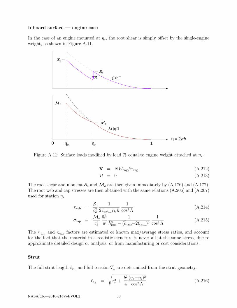
Inboard surface — engine case
In the case of an engine mounted at ηs, the root shear is simply offset by the single-engineweight, as shown in Figure A.11.
η = 2 y/b 1η0 o ηs
(η)
(η)s
s
o
o
Figure A.11: Surface loads modified by load R equal to engine weight attached at ηs.
R = NWeng/neng (A.212)
P = 0 (A.213)
The root shear and moment So andMo are then given immediately by (A.176) and (A.177).The root web and cap stresses are then obtained with the same relations (A.206) and (A.207)used for station ηs.
τweb =So
c2o
1
2 twebo rh h
1
cos2 Λ(A.214)
σcap =Mo
c3o
6h
w
1
h3rms − (hrms−2tcapo
)3
1
cos4 Λ(A.215)
The rτweband rσcap factors are estimated or known max/average stress ratios, and account
for the fact that the material in a realistic structure is never all at the same stress, due toapproximate detailed design or analysis, or from manufacturing or cost considerations.
Strut
The full strut length ℓs⊥ and full tension T⊥ are determined from the strut geometry.
ℓs⊥ =
√
z2s +
b2
4
(ηs−ηo)2
cos2 Λ(A.216)
NASA/CR—2010-216794/VOL2 30

T⊥ = T ℓs⊥
ℓs(A.217)
The strut stress is then simply related to T⊥ and the strut cross-sectional area Astrut.
σstrut =T⊥
Astrut(A.218)
A.2.9 Surface Weights
Surface material volumes and volume moments
The surface structural weight is obtained directly from the total volume of the caps and webs,and the corresponding material densities. The volume V of any element of the swept surfaceis computed using the element’s normalized cross sectional area A, and the local streamwisechord c(η). The volume x-moment offsets ∆xV from the center box are also computed formass-centroid calculations. The volume y-moment offsets ∆yV from yo or ys are computedfor their contributions to the structural shear bending moment (A.174) and (A.175).
dy⊥ =dy
cos Λ=
b
2
dη
cos Λ(A.219)
A = A c2⊥
= A c2 cos2 Λ (A.220)
V =∫
A dy⊥ =b
2
∫
Ac2 cos Λ dη (A.221)
∆xV =∫
A (x−xwbox) dy⊥ =b2
4
∫
Ac2 (η−ηo) sin Λ dη (A.222)
∆yV =∫
A (y − yo) dy⊥ =b2
4
∫
Ac2 (η−ηo) cos Λ dη (A.223)
Using the assumed three-panel chord distribution (A.121), the unit-area (A=1) volume andvolume moments evaluate to the following for each of the three panels of one wing half.
Vcen =b
2
∫ ηo
0c2 dη = c2
o
b
2ηo (A.224)
Vinn =b
2
∫ ηs
ηo
c2 cos Λ dη = c2o
b
6(1 + λs+λ2
s)(ηs−ηo) cos Λ (A.225)
Vout =b
2
∫ 1
ηs
c2 cos Λ dη = c2o
b
6(λ2
s+λsλt+λ2t )(1−ηs) cos Λ (A.226)
∆xVinn =b2
4
∫ ηs
ηo
c2 (η−ηo) sin Λ dη = c2o
b2
48(1 + 2λs+3λ2
s)(ηs−ηo)2 sin Λ (A.227)
∆xVout =b2
4
∫ 1
ηs
c2 (η−ηo) sin Λ dη = c2o
b2
48(λ2
s+2λsλt+3λ2t )(1−ηs)
2 sin Λ
+ c2o
b2
12(λ2
s + λsλt + λ2t )(ηs−ηo)(1−ηs) sin Λ (A.228)
∆yVinn =b2
4
∫ ηs
ηo
c2 (η−ηo) sin Λ dη = c2o
b2
48(1 + 2λs+3λ2
s)(ηs−ηo)2 cos Λ (A.229)
∆yVout =b2
4
∫ 1
ηs
c2 (η−ηs) sin Λ dη = c2o
b2
48(λ2
s+2λsλt+3λ2t )(1−ηs)
2 cos Λ (A.230)
NASA/CR—2010-216794/VOL2 31

Surface weights and weight moments
For the structural sizing calculations it’s necessary to determine the contributions of thestructure and fuel separately for the inner and outer panels. These are calculated by applyingthe material densities and actual area ratios to the unit-area volumes calculated previously.
Acapinn=
Acapo+ Acaps
λ2s
1 + λ2s
(A.231)
Awebinn=
Awebo + Awebsλ2s
1 + λ2s
(A.232)
Wscen =[
ρcap Acapo+ ρweb Awebo
]
g Vcen (A.233)
Wsinn =[
ρcap Acapinn+ ρweb Awebinn
]
g Vinn (A.234)
∆xWsinn =[
ρcap Acapinn+ ρweb Awebinn
]
g ∆xVinn (A.235)
∆yWsinn =[
ρcap Acapinn+ ρweb Awebinn
]
g ∆yVinn (A.236)
Wsout =[
ρcap Acaps+ ρweb Awebs
]
g Vout (A.237)
∆xWsout =[
ρcap Acaps+ ρweb Awebs
]
g ∆xVout (A.238)
∆yWsout =[
ρcap Acaps+ ρweb Awebs
]
g ∆yVout (A.239)
Wfcen = ρfuel Afuelo g Vinn (A.240)
Afuelinn=
Afuelo + Afuelsλ2s
1 + λ2s
(A.241)
Wfinn = ρfuel Afuelinng Vinn (A.242)
∆xWfinn = ρfuel Afuelinng ∆xVinn (A.243)
∆yWfinn = ρfuel Afuelinng ∆yVinn (A.244)
Wfout = ρfuel Afuels g Vout (A.245)
∆xWfout = ρfuel Afuels g ∆xVout (A.246)
∆yWfout = ρfuel Afuels g ∆yVout (A.247)
Assuming chord2-weighted average areas Ainn over the inner panel is deemed to be adequatefor approximating the material and fuel volumes, since Ao and As will be very similar forany reasonable wing/strut configuration, and in fact are equal for the small taper ratiocantilevered wing case like for the outer panel.
The total structural wing weight and x-moment is obtained by summing the weights forall the panels for the two wing halves, with added wing weight accounted for by the fwadd
fraction components.
fwadd = fflap + fslat + faile + flete + fribs + fspoi + fwatt (A.248)
Wwing = 2 (Wscen + Wsinn + Wsout) (1+fwadd) (A.249)
∆xWwing = 2 (∆xWsinn + ∆xWsout) (1+fwadd) (A.250)
NASA/CR—2010-216794/VOL2 32

The maximum (volume-limited) wing fuel weight and x-moment is computed the same way.
Wfmax = 2 (Wfcen + Wfinn + Wfout) (A.251)
∆xWfmax = 2 (∆xWfinn + ∆xWfout) (A.252)
This can be modified if only some of the wingbox volume is chosen to hold fuel.
Total panel weights
The wing structural shear and bending moment relations (A.174) – (A.177) require theweights and weight y-moments of the individual wing panels. These are assembled by sum-ming the structure’s and maximum fuel’s weight contributions derived previously, with thelatter simply scaled by the max-fuel usage fraction rfmax.
rfmax =Wfuel
Wfmax
(A.253)
Winn = Wsinn(1+fwadd) + rfmax Wfinn (A.254)
Wout = Wsout(1+fwadd) + rfmax Wfout (A.255)
∆yWinn = ∆yWsinn(1+fwadd) + rfmax ∆yWfinn (A.256)
∆yWout = ∆yWsout(1+fwadd) + rfmax ∆yWfout (A.257)
Using a single rfmax value assumes the partial fuel load is uniformly distributed percentage-wise in all the available volume. Of course, rfmax could be varied between the panels to reflectother fuel distributions.
Strut weight
The weight of the strut is computed directly from its cross-sectional area and total lengthfor the two sides.
Wstrut = ρstrut gAstrut 2ℓs⊥ (A.258)
∆xWstrut =b
4(ηs−ηo) tanΛ Wstrut (A.259)
Wingbox component weights
The overall sparcap and web weights for the entire wing can also be determined, althoughthese are merely informative and are not needed for any other calculations.
Wcap = 2ρcap g[
AcapoVcen + 1
2
(
Acapo+Acaps
)
Vinn + AcapsVout
]
(A.260)
Wweb = 2ρweb g[
AweboVcen + 12
(
Awebo +Awebs
)
Vinn + AwebsVout
]
(A.261)
NASA/CR—2010-216794/VOL2 33

Tail surface weight
All the wing wing stress and weight analyses above apply equally to the vertical and hori-zontal tail surfaces, with the appropriate span and load definitions. It is assumed that nostrut is used, so that
csh= coh
(A.262)
bsh= boh
(A.263)
and likewise for the vertical tail. The main difference is the derivation of the root loadingmagnitude po, which is set by the maximum design loads at qNE, defined by (A.72) and(A.74). Specifically, we have
poh=
Lhmax
bh
2
1+λh
(A.264)
where the ()h subscript denotes the horizontal tail/ The same relation is used for the verticaltail. Gravity and inertial loads are neglected here, since for tails they are typically muchsmaller than the airloads at qNE. Of course, they could be included as was done for the wing.With the tail po values defined, the structural-box sizing and weight estimation proceedsusing the same relations as for the wing, starting with So. The vertical tail is treated byassuming its mirror image exists, so that the b value in (A.174) and (A.175) is actually twicethe actual vertical tail span. No other adjustments need to be made. The net result is theoverall horizontal and vertical tail weights, and tail weight moments.
→ Whtail (A.265)
→ Wvtail (A.266)
→ ∆xWhtail (A.267)
→ ∆xWvtail (A.268)
A.2.10 Engine System Weight
The bare engine weight Webare is calculated using an assumed dependence on the enginedesign core mass flow mD, overall design pressure ratio OPRD, and the design bypass ratioBPRD. The model’s constants have been calibrated with listed weights for existing turbofans.The added weight Weadd, specified via the empirical fraction feadd, accounts for the fuelsystem and miscellaneous related equipment.
Webare = neng We1(mD, OPRD, BPRD) (A.269)
Weadd = Webare feadd (A.270)
The nacelle plus thrust reverser weight is calculated using an assumed dependence on theengine fan diameter df and the nacelle surface area, the latter being specified by the empiricalarea ratio rSnace relative to the fan area.
Snace1 = rSnaceπ
4d2
f (A.271)
Wnace = neng Wn1 (df , Snace1) (A.272)
NASA/CR—2010-216794/VOL2 34

The pylon weight Wpylon, specified via the empirical fraction fpylon, accounts for the pylonand other mounting structure.
Webare = neng We1(mD, OPRD, BPRD) (A.273)
Wpylon = (Webare + Weadd + Wnace) fpylon (A.274)
The total engine system weight and weight moment is then defined as follows. The engineweight fraction is also defined, and is used in the overall weight iteration procedure.
Weng = Webare + Weadd + Wnace + Wpylon (A.275)
xWeng = xeng Weng (A.276)
feng =Weng
WMTO
(A.277)
A.2.11 Moments and Balance
Weight moment and aerodynamic moment calculations are used to size the horizontal tail tomeet stability or trim-limit requirements, to determine allowable CG limits, and to determinethe required pitch-trim tail lift.
Overall weight moment
The overall flying weight is summed as follows. Partial payload and partial fuel are specifiedwith the arbitrary rpay and rfuel ratios relative to maximum design values.
W = rpayWpay + rfuelWfuel
+ Wfuse + Wwing + Wstrut + Whtail + Wvtail
+ Weng + Whpesys + Wlgnose + Wlgmain (A.278)
The partial passenger payload distribution in the cabin is specified by the parameter ξpay
which can take on any value 0 . . . 1. Specific instances are
ξpay =
0.0 , passengers packed towards the front0.5 , passengers centered in cabin1.0 , passengers packed towards the back
(A.279)
This then determines the passenger payload weight centroid xpay.
xcabin = 12(xshell 1 + xshell 2) (A.280)
lcabin = xshell 2 − xshell 1 (A.281)
xpay = xcabin + lcabin
(
ξpay − 12
)
(1− rpay) (A.282)
Note that with a full passenger load, rpay =1, the mass centroid is always at the center pointxcabin, regardless of ξpay. The overall aircraft weight moment is then computed as follows.
xW = rpay xpayWpay
NASA/CR—2010-216794/VOL2 35

+ rfuel (xwboxWfuel + ∆xWfuel)
+ xWfuse
+ xwboxWwing + ∆xWwing
+ xwboxWstrut + ∆xWstrut
+ xhtailWhtail + ∆xWhtail
+ xvtailWvtail + ∆xWvtail
+ xWeng
+ xhpesysWhpesys
+ xlgnoseWlgnose
+ xlgmainWlgmain (A.283)
The aircraft CG location then follows.
xCG =xW
W(A.284)
Overall aerodynamic moment
The overall aerodynamic pitching moment about the origin comes from the wing, the hori-zontal tail, and the fuselage. For simplicity, the wing root chord co is used as the referencemoment arm rather than the more traditional m.a.c.
CM ≡ M12ρV 2
∞Sco
= CMw0 +(
CMw1 −xwbox
co
)(
CL −Sh
SCLh
)
+Sh coh
S coCMh0 +
(
coh
coCMh1 −
xhbox
co
)
Sh
SCLh
+CMV f 1
Sco(CL − CLMf 0
) (A.285)
and CMV f 1 and CLMf 0give the fuselage’s pitching moment volume dependence on aicraft CL.
Mfuse12ρV 2
∞
≡ CMV f = CMV f 1 (CL − CLMf 0) (A.286)
From slender body theory, a fuselage of volume Vf isolated from the wing has
CMV f ≃ 2Vf (α− αMf 0) (A.287)
CMV f 1 ≃2Vf
dCL/dα(A.288)
but this will typically be considerably modified by the interaction with the wing. Ragardless,the aircraft center of pressure (or lift centroid) is given as follows.
xCP = −co CM
CL(A.289)
NASA/CR—2010-216794/VOL2 36

Neutral point
The neutral point is estimated by first translating the aerodynamic pitching moment (A.285)to some arbitrary reference x location.
CM(x) = CM +x
coCL (A.290)
The neutral point is the x location which makes (A.290) stationary with respect to CL, or
∂CM (xNP )
∂CL=
∂CM
∂CL+
xNP
co= 0 (A.291)
xNP = −co∂CM
∂CL(A.292)
where co∂CM
∂CL= (coCMw1 − xwbox)
(
1 − Sh
S
∂CLh
∂CL
)
+ (cohCMh1 − xhbox)Sh
S
∂CLh
∂CL
+CMV f 1
S(A.293)
Pitch trim requirement
Every operating point must meet the requirement of pitch trim, which is equivalent to thecenters of weight and pressure cooinciding. This is enforced by requiring that the followingtotal-moment residual is zero.
RM(xwbox, Sh, CLh, CL, rfuel, rpay, ξpay) ≡ xCG − xCP =xW
W+
co CM
CL= 0 (A.294)
The argument list of the residual indicates the variables which have the strongest influenceon pitch trim.
Pitch stability requirement
An aircraft must also have some minimum amount of static pitch stability, which meansthat the rearmost center of gravity must be ahead of the neutral point by the static marginfraction fSM of the mean aerodynamic chord. This is met when the following stability residualis zero.
RS(xwbox, Sh, rfuel, rpay, ξpay) ≡ xCG − xNP + fSM cMA = 0 (A.295)
The argument list indicates the variables which have the strongest influence on pitch stability.
A.2.12 Tail Sizing
The tail areas can be sized by a number of alternative requirements. The most commonapproaches are outlined here.
NASA/CR—2010-216794/VOL2 37

Specified tail volumes
This is the simplest approach. The stability margin or damping requirements are assumedto be quantified by the horizontal and vertical tail volumes,
lh = xhtail − xwing (A.296)
lv = xvtail − xwing (A.297)
Vh =Sh
S
lhcmac
(A.298)
Vv =Sv
S
lvb
(A.299)
which when specified give the necessary Sh or Sv. Defining the tail arms from the center ofwing centroid rather than from the CG or the wing’s aerodynamic center is reasonable forthese rather simple sizing relations.
Design-case: Horizontal tail sizing and wing positioning
For the design case, both Sh and xwbox are determined so as to drive the pitch trim andstability residuals (A.294) and (A.295) to zero simultaneously. Their remaining argumentsare set for the appropriate worst-case situations:
RM = RM(xwbox, Sh ; (CLh)min, (CL)max, (rfuel)fwd, (rpay)fwd, 0) = 0 (A.300)
RS = RS(xwbox, Sh ; (rfuel)aft, (rpay)aft, 1) = 0 (A.301)
Specifically, for pitch trim the most-forward CG and most-negative flaps-down wing airfoilcm, at maximum flight CL are assumed. For stability the most-aft CG is assumed. The rpay
values which give the extreme forward and aft CG locations are obtained by solving theextremizing relation
∂RM
∂rpay= 0 (A.302)
which is a quadratic for rpay. It is solved twice, with ξpay = 0 chosen to give (rpay)fwd, andthen ξpay = 1 chosen to give (rpay)aft. Zero fuel, or rfuel = 0 is assumed for both cases, asthis typically gives the most extreme CG locations together with the worst-case payloaddistributions.
The two residuals (A.300) and (A.301) are simultaneously driven to zero by varying the wingposition xwbox and the horizontal tail area Sh, by solving the 2×2 Newton system. The fourJacobian elements are readily calculated.
∂RM
∂Sh
∂RM
∂xwbox
∂RS
∂Sh
∂RS
∂xwbox
δSh
δxwbox
= −
RM
RS
(A.303)
NASA/CR—2010-216794/VOL2 38

Off-design case: Tail lift setting
For off-design calculations where the wing location and horizontal tail area is set, pitch trimis achieved by adjusting CLh
. The pitch-trim residual (A.294) is therefore driven to zero witha Newton step on CLh
.
∂RM
∂CLh
=1
CL
[
−(coCM1 − xwbox)Sh
S+ (cohCMh1 − xhbox)
Sh
S
]
(A.304)
(CLh)new = CLh
− RM
∂RM/∂CLh
(A.305)
Vertical tail sizing via engine-out yaw power
An alternative to the specified vertical tail volume (A.299) is to size the vertical tail so thatit can achieve yaw trim with one engine out. The requirement is
qminCLvyawSv lv = (Feng + qminCDengAeng) yeng (A.306)
where qmin is the minimum takeoff dynamic pressure, CLvyaw is the maximum lift coefficientof the vertical tail with some yaw control margin, Feng is the thrust of one engine, CDeng isthe drag coefficient of a windmilling engine with reference area Aeng, and yeng is the lateraldistance of the outermost engine from the centerline.
A.2.13 Dissipation (Drag) Calculation
Power-based formulation
The performance calculations used here are based on the power balance and dissipationanalysis of Drela [12]. In brief, the usual streamwise force balance equation in constant-velocity flight is replaced with the power balance relation
F ′V∞ = D′V∞ + Wh (A.307)
where h is the climb rate, F ′ is an effective thrust, and D′ is an effective drag. Thesetwo effective forces are actually defined in terms of the net propulsive power and the netdissipation and vortex kinetic energy loss rate.
F ′V∞ ≡ PKinl+ PV + PKout − Φjet (A.308)
D′V∞ ≡ Φsurf + Φwake + Evortex (A.309)
The advantage of this power-balance approach is that it naturally handles the presence ofboundary layer ingestion (BLI) without the ambiguities or complications which arise witha force-balance approach. If no BLI is present then the two approaches become entirelyequivalent, and F ′, D′ become the conventional thrust and drag F, D. The BLI accountingis described in more detail in the separate document “Power Accounting with BoundaryLayer Ingestion”. Only the relevant results will be used here.
NASA/CR—2010-216794/VOL2 39

The disspation and power loss terms in the above power equations are used to define thefollowing convenient coefficients.
C ′
Dp≡ Φsurf + Φwake
12ρV 3
∞S
(A.310)
C ′
Di≡ Evortex
12ρV 3
∞S
= CDi(A.311)
C ′
D ≡ D′V∞
12ρV 3
∞S
= C ′
Dp+ CDi
(A.312)
As with “F” and “D”, the “CD” notation is used as a reminder that if there is no BLI, theabove definitions reduce to the conventional drag coefficients and the primes can be simplydropped in that case.
In the following subsections, the various contributions to the overall power-loss coefficientC ′
D will be computed. Most of these rely on traditional drag models and terminology, hencethe “Drag” label will be used in the sections titles, mostly out of habit. As a useful indicator,the prime ()′ will be retained only for those contributions which are potentially influenced byBLI. Unprimed contributions will thus also correspond to the conventional drag coefficients.
Fuselage Profile Drag
The fuselage profile drag is determined by an pseudo-axisymmetric viscous/inviscid calcu-lation method, which is described in the separate document “Simplified Viscous/InviscidCalculation for Nearly-Axisymmetric Bodies”. This gives reliable viscous flow and fuselagedrag predictions for any reasonable fuselage shape, without the need to rely on effectivewetted area or fineness-ratio correlations.
The method requires the geometry to be specified in the form of a cross-sectional areadistribution A(x) and also a perimeter distribution b0(x), shown in Figure A.12. For a roundcross-section these are of course related, but to allow treating more general fuselage cross-sections, they are assumed to be specified separately. The cross section sizes and shapes canvary along the body, provided the variation is reasonably smooth.
x
b
A(x)
(x)∆∗ ∗ΘΘ, ,
A(x)
(x)
y
z ∗ ∗, , (x)δ θ θ
0
Figure A.12: Fuselage defined by cross-sectional area A(x) and perimeter b0(x) distribu-tions. Viscous calculation produces displacement, momentum, and kinetic energy areas∆∗, Θ, Θ∗
(x).
NASA/CR—2010-216794/VOL2 40

The cross-sectional area over the center cylindrical portion is Afuse, which has already beendefined by (A.6). This also defines the radius of the equivalent round cylinder.
Rcyl =
√
Afuse
π(A.313)
The equivalent radii over the tapering nose and radius are then defined via the followingconvenient functions.
R(x) =
Rcyl
[
1−(
xblend1−x
xblend1−xnose
)a ]1/a
, xnose < x < xblend1
Rcyl , xblend1 < x < xblend 2
Rcyl
1−(
x−xblend 2
xend−xblend 2
)b
, xblend 2 < x < xtail
(A.314)
a ≃ 1.6 (A.315)
b ≃ 2.0 (A.316)
The xblend1and xblend 2
locations are the nose and tailcone blend points, and do not necessarilyhave to be exactly the same as the xshell1 and xshell 2 locations which define the loaded pressureshell. Likewise, xend is the aerodynamic endpoint of the tailcone, and is distinct from itsstructural endpoint xconend. The a and b constant values above give reasonable typicalfuselage shapes.
If the fuselage is nearly round, the necessary area and perimeter distributions follow imme-diately.
A(x) = π R(x)2 (A.317)
b0(x) = 2πR(x) (A.318)
This would be suitably modified for non-circular cross-sections.
With this geometry definition, the viscous/inviscid calculation procedure provides the mo-mentum and kinetic energy area distributions along the body and wake,
{Θ(s) , Θ∗(s)} = ffexcr F(M∞, Reℓ ; A(x), b0(x)) (A.319)
where F denotes the overall viscous/inviscid calculation procedure, and ffexcr ≥ 1 is anempirical factor to allow for fuselage excrescence drag sources.
Specific values of interest are the far-downstream momentum area Θwake at the wake end-point, and the kinetic energy area ΘTE at the body endpoint or trailing edge.
Θwake = Θ(swake) (A.320)
Θ∗
TE= Θ∗(sTE) (A.321)
The fuselage surface + wake dissipated power in the absence of BLI is then evaluated asfollows, consistent with the usual wake momentum defect relations.
CDfuse≡ Φfuse
12ρV 3
∞S
=Φsurf + Φwake
12ρV 3
∞S
(without BLI) (A.322)
CDfuse=
Dfuse12ρV 2S
=2Θwake
S(without BLI) (A.323)
NASA/CR—2010-216794/VOL2 41

If BLI is present at or near the trailing edge, the upstream boundary layer and correspondingsurface dissipation Φsurf will be mostly unaffected. But the viscous fluid flowing into thewake is now reduced by the ingestion fraction fBLI f
, so that the wake dissipation Φwake willbe reduced by the same fraction. This then gives the following overall fuselage dissipationcoefficient for the BLI case.
C ′
Dfuse≡ Φfuse
12ρV 3
∞S
=Φsurf + Φwake(1−fBLI f
)12ρV 3
∞S
(with BLI) (A.324)
C ′
Dfuse= CΦsurf
+ CΦwake(1−fBLI f
) = CDfuse− CΦwake
fBLI f(with BLI) (A.325)
where CΦsurf=
Θ∗
TE
S(A.326)
CΦwake=
2Θwake
S− Θ∗
TE
S(A.327)
Wing Profile Drag
The power dissipated in the wing’s surface and wake for the non-ingesting case defines thewing’s profile drag coefficient.
CDwing≡ Φwing
12ρV 3
∞S
=Φsurf + Φwake
12ρV 3
∞S
(without BLI) (A.328)
Any ingestion of the wing boundary layer is captured by the ingestion fraction fBLI w , in thesame manner as for the fuselage.
C ′
Dwing≡ Φwing
12ρV 3
∞S
=Φsurf + Φwake(1−fBLIw)
12ρV 3
∞S
(with BLI) (A.329)
C ′
Dwing= CDwing
− CΦwakefBLI w (with BLI) (A.330)
where CΦwake≃ rΦwake
CDwing(A.331)
rΦwake≃ 0.15 (A.332)
The wake dissipation is assumed here to be rΦwake=15% of the total airfoil dissipation, which
is typical of optimized modern transonic airfoils.
The actual calculation of CDwingis via the drag using infinite swept wing theory, which
also gives the lift in term of the perpendicular-plane velocity V⊥ and lift coefficient cℓ⊥.Figure A.13 shows the relations. These quantities are related to the local loading via
V⊥ = V∞ cos Λ (A.333)
dL = p dy = 12ρV 2
⊥c⊥ cℓ⊥ dy⊥ (A.334)
po P (η) = 12ρV 2
∞co C(η) cℓ⊥(η) cos2 Λ (A.335)
excluding the wing center and extreme tip where the lift adjustements ∆Lo and ∆Lt arelocated. The loading scale po in level flight is obtained from (A.159) with N =1 as follows.
W = L = 12ρV 2
∞S CL (A.336)
Lhtail = 12ρV 2
∞Sh CLh
(A.337)
po =1
Kp b(L− Lhtail) (A.338)
NASA/CR—2010-216794/VOL2 42

Using (A.338) to substitute for po in (A.335) and rearranging gives an explicit expression forthe local section lift coefficient.
CLhtail=
Sh
SCLh
(A.339)
cℓ⊥(η) =CL − CLhtail
cos2 Λ
S
Kp b co
P(η)
C(η)(A.340)
Λ VV
Df
DpDp
shockpotential flow streamline
Cp lc
M fdc
dc p
Figure A.13: Friction and pressure drag forces on infinite swept wing
Using this cℓ⊥ and also M⊥, the perpendicular-plane friction and pressure drag coefficientsare then obtained from a 2D airfoil drag database having the form
cdf= fwexcr cdf
(cℓ⊥, M⊥, tc)(
Rec
Reref
)aRe
(A.341)
cdp = fwexcr cdp(cℓ⊥, M⊥, tc)(
Rec
Reref
)aRe
(A.342)
where M⊥ = M∞ cos Λ (A.343)tc
= h (A.344)
Rec =ρ∞V∞ c
µ∞
(A.345)
aRe ≃ −0.15 (A.346)
and fwexcr ≥ 1 is an empirical specified factor to account for wing excrescence drag sources,and Reref is a reference Reynolds number at which the database functions cdf
, cdp were com-puted. The chord Reynolds number Rec could of course be treated as an additional parameterin the database, but at a considerable increase in the size of the database and the compu-tational effort needed to construct it. The value of the Re-scaling exponent aRe ≃ −0.15 isappropriate for fully-turbulent flow.
Note that the database includes the airfoil thickness/chord ratio tc
= h, which is crucial forobtaining a realistic wing thickness/sweep/CL/Mach tradeoff. The thickness dependence isdetermined by viscous MSES [18] calculations on a number of transonic airfoils or varyingthickness, such as the ones shown in Figure A.14. Each airfoil has been designed indepen-dently for a well-behaved transonic drag rise, so that the database returns cdf
and cdp values
NASA/CR—2010-216794/VOL2 43

representative of the best transonic airfoil technology. A piecewise-linear airfoil thicknessdistribution is assumed, defined by the three values ho, hs, ht.
h(η) =
ho , 0<η<ηo
ho + (hs−ho)η−ηo
ηs−ηo, ηo <η<ηs
hs + (ht−hs)η−ηs
1 −ηs
, ηo <η<ηs
(A.347)
On typical transport wings most of the thickness/chord variation occurs inboard, so in thatcase, only ho and hs would be considered as design variables, and ht = hs would be assumed.
Figure A.14: Airfoil family used to generate airfoil-performance database.
The 2D profile drag coefficients are applied to the swept wing using infinite swept-wingtheory, illustrated in Figure A.13. This treatment is exact for laminar flow on untaperedwings, and quite accurate for turbulent flow. The friction drag is assumed to scale withfreestream dynamic pressure and to act mostly along the freestream flow direction, whilethe pressure drag from the shock and viscous diplacement is assumed to scale with thewing-normal dynamic pressure and to act normal to the wing-spanwise axis. The total localstreamwise drag element is then given as follows.
dDwing = dDf + dDp = dDf + dDp⊥ cos Λ
= 12ρV 2
∞c cd dy (A.348)
cd = cdf + cdp cos3Λ (infinite swept wing) (A.349)
However, this relation is not realistic near the fuselage. Here the potential flow is forcedparallel to the freestream direction which causes the wing shock to become locally unswept,as shown in Figure A.15. Also, the full streamwise dynamic pressure (as opposed to thewing-normal dynamic pressure) acts at the trailing edge where most of the displacement-effect pressure drag occurs. Hence, the sweep correction is dropped off towards the fuselagevia the heuristic “unsweep” function fSuns(η).
cd(η) ={
cdf + cdp
[
fSuns + (1−fSuns) cos2Λ]
cos Λ}
(actual swept wing) (A.350)
fSuns(η) = exp(
− 1
kSuns
y−yo
c
)
= exp
(
− 1
kSuns
η−ηo
C(η)
b
2co
)
(A.351)
kSuns ≃ 0.5 (A.352)
NASA/CR—2010-216794/VOL2 44

The kSuns decay constant controls the area of the wing most influenced by the shock unsweepcorrection, as shown in Figure A.15.
oc
2ok c
shock
potential flow streamlines
( unswept−shock wing portion )Suns
Figure A.15: Wing shock unsweeps near the fuselage, roughly over the area kunsc2o.
The overall wing profile drag is then obtained by numerical integration of (A.348), using(A.350) for the cd(η) function and (A.121) for the chord c(η) function.
CDwing≡ Dwing
12ρV 2
∞S
=bco
S
∫ 1
ηo
cd(η) C(η) dη (A.353)
Tail Profile Drag
The viscous dissipation of the tail surfaces is computed using the same relations as for thewing, giving the equivalent tail drag coefficients CDhtail
and CDvtail. No BLI is assumed, but
could be included in the same manner as for the wing. Because tail surfaces typically donot have significant shock waves, the shock-unsweep correction (A.350) is inappropriate.Instead, the 2D friction and pressure drag coefficients cdf
and cdp are specified directly andare used in the infinite-wing relation (A.349), and are assumed constant over the surface sothat numerical spanwise integration is unnecessary.
CDhtail= cdfh
+ cdphcos3Λh (A.354)
CDvtail= cdfv
+ cdpv cos3Λv (A.355)
Strut Profile Drag
In the absence of any BLI on the strut, its dissipation is fully captured by its conventionaldrag coefficient, scaled by the local mean-cube-average velocity ratio rV strut to allow for thefact that a strut is typically in the decreased flow velocity below a lifting wing. Simple sweepcorrections are also used as for the wing.
cstrut =
√
Astrut
kA hstrut
, kA ≃ 0.65 (A.356)
Sstrut = 2cstrut ℓs⊥ (A.357)
NASA/CR—2010-216794/VOL2 45

cos Λs =ℓs
ℓs⊥
(A.358)
CDstrut =Sstrut
S
(
cdfs+ cdps cos3Λs
)
r3V strut
(A.359)
Picking a strut thickness/chord ratio hstrut ≃ 0.15 . . . 0.20 typically gives the minimum overalldrag for a given strut cross-sectional area Astrut. The kA area factor of 0.65 is typical of mostsymmetric airfoils.
Engine Nacelle Profile Drag
The nacelle viscous dissipation accounts for the external nacelle flow only, since the internalflow is represented by the engine diffuser and nozzle losses. The external wetted area andcorresponding area fraction is determined as an assumed fraction rSnace of the engine fanarea.
Snace = neng rSnaceπ
4d2
fan (A.360)
fSnace =Snace
S(A.361)
The skin friction coefficient can also be calculated based on the nacelle-length Reynoldsnumber and a standard turbulent skin-friction law, with an excrescence factor fnexcr ≥ 1included as for the fuselage and wing.
ℓnace = 0.15 rSnace dfan (A.362)
Renace =ρ∞V∞ℓnace
µ∞
(A.363)
Cfnace = fnexcr Cfturb(Renace) (A.364)
The nacelle is assumed to be immersed in the potential nearfield of a nearby wing or fuselage,with a local effective freestream Vnace which differs somewhat from the true freestream V∞,and is specified via the ratio Vnace/V∞. Depending on the flight condition and engine power,the fan-face Mach number M2 will in general differ considerably from the corresponding localM ′
∞, The nacelle is therefore effectively a loaded ring airfoil, which can be represented by a
ring vortex sheet whose resulting external nacelle-surface velocity is approximately
VnLE≃ 2Vnace − V2 (A.365)
Vnace
V∞
= rV nace (A.366)
VnLE
V∞
= 2Vnace
V∞
− V2
V∞
≃ max(
2rV nace −M2
M∞
, 0)
(A.367)
at the lip, as sketched in Figure A.16. Limiting VnLEabove zero avoids unrealistic results
for low airspeed, high-power operation situations.
Assuming a linear acceleration or deceleration from VnLEto Vnace at the nacelle nozzle gives
the following mean-cube velocity ratio on the nacelle surface.
r3V nsurf
≡ 1
V 3∞
∫ 1
0
[
Vnace + (VnLE− Vnace) (1−ξ)
]3dξ (A.368)
NASA/CR—2010-216794/VOL2 46

V
V2
nacelle dissipation
V2
V
V Vnace
nLE
Vnace
VnLE
Figure A.16: Velocity distribution on inside and outside of engine nacelle. Outside velocitydetermines nacelle dissipation and implied nacelle drag. The VnLE
>V2 case shown is for atypical cruise condition, while VnLE
<V2 will occur at low speeds and high power.
=1
4
[
VnLE
V∞
+ rV nace
]
[
(
VnLE
V∞
)2
+ r2V nace
]
(A.369)
The nacelle-surface dissipation, expressed as the equivalent nacelle drag coefficient, is nowestimated using a turbulent wetted-area skin-friction coefficient, weighted by the mean-cubevelocity ratio.
CDnace = fSnace Cfnace r3V nsurf
(A.370)
Induced Drag
The induced drag is calculated using a discrete vortex Trefftz-Plane analysis. The circulationof the wing wake immediately behind the trailing edge is
Γwing(η) =p(η)
ρV∞
≃ p(η)
ρV∞
√
1−ηkt (A.371)
kt ≃ 16 (A.372)
where the approximation realistically represents the tip lift rolloff for typical taper ratios,and is consistent with the assumed fLt ≃ −0.05 value for the tip lift loss factor. Thiscirculation is convected into the wake along streamlines which will typically constrict behindthe fuselage by continuity. Figure A.17 shows two possible aft fuselage taper shapes, givingtwo different wake constrictions.
An annular streamtube at the wing contracts to another annular streamtube in the wakewith the same cross-sectional area. The y and y′ locations on the wing and wake which areconnected by a streamline are therefore related by the correspondence function.
y′(y) =
√
y2 − y2o + y′
o2 (A.373)
NASA/CR—2010-216794/VOL2 47

( )
/2by
y’ /2b’y’
y
y’o
yo /2b
/2b’y’
y
y’o
yo
Γ y’( )
Γ ywing
Figure A.17: Wake streamline contraction due to fuselage thickness, carrying wing circulationinto the wake. Two shaded streamtubes are shown. Wake center radius y′
o is nonzero due tothe fuselage viscous wake displacement area.
The Trefftz Plane circulation Γ(y′) is then given by the coordinate shift. The mappingfunction y′
(y) is not defined for y<yo, so the circulation there is simply set from the yo value.
Γwake(y′) =
{
Γwing (y(y′)) , y>yo
Γwing (yo)(A.374)
The Trefftz Plane analysis uses point vortices. The circulation (A.374) is evaluated at themidpoints of n intervals along the wake trace, spaced more or less evenly in the Glauert angleto give a cosine distribution in physical space. The wake’s vertical z positions are simplytaken directly from the wing.
θi+1/2 =π
2
i− 1/2
n, i = 1 . . . n (A.375)
yi+1/2 =b
2cos θi+1/2 (A.376)
y′
i+1/2 =√
y2i+1/2 − y2
o + y′o2 (A.377)
z′i+1/2 = zi+1/2 (A.378)
Γi+1/2 = Γwing(yi+1/2) (A.379)
The locations of n + 1 trailing vortices are computed similarly.
θi =π
2
i− 1
n, i = 1 . . . n+1 (A.380)
yi =b
2cos θi (A.381)
NASA/CR—2010-216794/VOL2 48

y′
i =√
y2i − y2
o + y′o2 (A.382)
z′i = zi (A.383)
The circulations of these trailing vortices are the differences of the adjacent bound circula-tions, with the circulation beyond the tips effectively zero.
Γi =
−Γi−1/2 , i = 1 (left tip)Γi+1/2 − Γi−1/2 , i = 2 . . . nΓi+1/2 , i = n+1 (right tip)
(A.384)
The above definitions are also applied to the horizontal tail, with its discrete points simplyappended to the list and n increased accordingly.
y’
z’
wi +1/2
i +1/2vΓi− Γi
−+1
Figure A.18: Trefftz Plane vortices i, i+1 . . . and collocation points i+1/2 used for velocity,impulse, and kinetic energy calculations. Left/right symmetry is exploited.
The Trefftz plane calculation proceeds by first calculating the y-z wake velocity componentsat the y′
i+1/2, z′
i+1/2 interval midpoints, induced by all the trailing vortices and their left-sideimages.
vi+1/2 =n+1∑
j=1
Γj
2π
−(z′i+1/2−z′j)
(y′
i+1/2−y′j)
2 + (z′i+1/2−z′j)2−
−(z′i+1/2−z′j)
(y′
i+1/2+y′j)
2 + (z′i+1/2−z′j)2
(A.385)
wi+1/2 =n+1∑
j=1
Γj
2π
y′
i+1/2−y′
j
(y′
i+1/2−y′j)
2 + (z′i+1/2−z′j)2−
y′
i+1/2+y′
j
(y′
i+1/2+y′j)
2 + (z′i+1/2−z′j)2
(A.386)
The overall lift and induced drag are then computed using the Trefftz Plane vertical impulseand kinetic energy. The sums are doubled to account for the left side image.
CLTP=
212ρV 2
∞S
n∑
i=1
ρV∞ Γi+1/2 (y′
i+1 − y′
i) (A.387)
CDTP=
212ρV 2
∞S
n∑
i=1
−ρ
2Γi+1/2
[
wi+1/2 (y′
i+1−y′
i) − vi+1/2 (z′i+1−z′i)]
(A.388)
To minimize any modeling and numerical errors incurred in the wake contraction model andthe point-vortex summations, the final induced drag value is scaled by the square of the
NASA/CR—2010-216794/VOL2 49

surface-integral and Trefftz-Plane drag values.
CDi= CDTP
(
CL
CLTP
)2
(A.389)
This is equivalent to using the Trefftz Plane analysis to calculate the span efficiency ratherthan the actual induced drag coefficient.
Total Drag
The total effective aircraft dissipation coefficient is obtained by summing all the contribu-tions.
C ′
D = CDi+ C ′
Dfuse+ C ′
Dwing+ CDhtail
+ CDvtail+ CDstrut + CDnace (A.390)
A.2.14 Engine Performance Model and Sizing
Engine model summary
The extensive details of the engine calculations are given in the separate documents “Tur-bofan Sizing and Analysis with Variable cp(T )” and “Film Cooling Flow Loss Model”. Thetreatment of the inlet kinetic energy defect Kinl is described in the document “Power Ac-counting with Boundary Layer Ingestion”. In brief, Kinl reduces the fan inlet total pressure,and also adds to the net effective thrust by the amount Kinl/V∞, which in engine parlancecan be interpreted as a reduction in inlet “ram drag”.
The engine model can be run in one of three modes:
1) Design sizing mode. The net thrust F ′
e and combustor exit temperature Tt 4 are specifiedalong with a number of other component and operating parameters, and the engine flowareas A2, A5 . . . are computed.
2) Off-design analysis mode. The areas and Tt 4 are prescribed, and thrust F ′
e is computed.
3) Off-design analysis mode. The areas and F ′
e are prescribed, and Tt 4 is computed.
For all three modes, the specific fuel consumption TSFC ′ and all other engine operatingparameters which are not specified are also computed.
{A2, A5... ; TSFC ′...} = Feng1
(F ′
e, Tt4 , OPRD, BPRD... ; M∞, p∞, T∞, Kinl...) (A.391)
{F ′
e ; TSFC ′, OPR, BPR...} = Feng2(Tt4 , A2, A5... ; M∞, p∞, T∞, Kinl...) (A.392)
{Tt4 ; TSFC ′, OPR, BPR...} = Feng3(F ′
e, A2, A5... ; M∞, p∞, T∞, Kinl...) (A.393)
where TSFC ′ ≡ F ′
e
mfuel g(A.394)
Kinl ≡(
12ρeV
3e Θ∗
)
inl=
fBLI f
neng
(
12ρeV
3e Θ∗
)
TE(A.395)
NASA/CR—2010-216794/VOL2 50

In these calculations, the fan inlet total pressure pt 2 is reduced as a result of the BLI. Areasonable estimate is
pt 2 = pt ∞ −Kinl
Vinl
(A.396)
Vinl =∫∫
inlV dA (A.397)
where Vinl is the fan face volume flow.
Engine Sizing
In the design mode 1), the specified thrust is obtained is determined from the start-of-cruiseweight Wc, lift/drag ratio, and the slight cruise-climb angle γCR.
F ′
D= rBc Wc
(
C ′
D
CL
+ γCR
)
c
(A.398)
F ′
eD=
F ′
D
neng(A.399)
The engine calculations determine the specific thrust
FspD≡ F ′
eD
a∞ mcore(1+BPRD)(A.400)
which then determines the core mass flow mcore and the associated fan flow area A2 and fandiameter df .
A2 =mcore(1+BPRD)
ρ2u2
=1
FspD
F ′
eD
γp∞
1
M2D
(
1 + γ−12
M22D
1 + γ−12
M2∞
)
γ+12(γ−1)
(A.401)
df =
√
4A2
π(1−HTR2f )
(A.402)
Similar calculations are used for the other component and nozzle areas.
A.2.15 Mission Performance and Fuel Burn Analysis
Mission profiles
The altitude, weight, and thrust profiles versus range are schematically shown in FigureA.19.
At any profile point these are related via the following normal force and axial force relations.
W sin γ = F ′ − D′ − W
g
dV
dt(A.403)
W cos γ = L (A.404)
NASA/CR—2010-216794/VOL2 51

hd
he
hc
hb
cR Rd
γ
cruise−climb
descentclimb
takeoff
h
WcW
Wd
WreserveW
b
e
W W= fuel−
= 0Rb
F
MTO
We W W= −MTO
dry MTO
total
CRγDE
R R=
W W=
burn
Figure A.19: Design-mission profiles of altitude, weight, thrust, versus range.
Equation (A.403) is merely a recast form of the power-balance equation (A.307), with theadded last acceleration term. The subscript has also been dropped from V∞ for convenience.
The flight speed at any profile point is obtained from a specified CL and ambient densityusing equation (A.404).
V =
√
2W cos γ
ρ S CL(A.405)
Some iteration is required with the thrust/drag relations below to determine the climb angleγ needed in (A.405).
Dividing (A.403) by (A.404), and using the kinematic ground-speed relation
dR
dt= V cos γ (A.406)
together with the fuel-burn to thrust relation
dW
dt= −mfuelg = −F ′ TSFC ′ (A.407)
gives an expression for the climb angle γ or the equivalent climb gradient dh/dR, and alsothe weight-loss gradient dW/dR.
tan γ =dh
dR=
F ′
W
1
cos γ− D′
L− 1
2g
d(V 2)
dR(A.408)
NASA/CR—2010-216794/VOL2 52

dW
dR= −F ′
TSFC ′
V cos γ(A.409)
These will be suitably integrated over the mission segments to obtain the altitude and weightprofiles h(R) and W (R).
The instantaneous climb or descent angle γ in the above expressions can be computed bycombining (A.403) and (A.404), and solving for the resulting quadratic equation for sin γ.
φ =F ′
W− V
g(A.410)
ǫ =C ′
D
CL
(A.411)
sin γ =φ− ǫ
√1− φ2 + ǫ2
1 + ǫ2(A.412)
The V acceleration term in the excess thrust-to-weight ratio φ can be neglected for mosttransport aircraft. The corresponding integrated d(V 2) differential in (A.408) is also typicallysmall, but there’s little reason to exclude it in calculations.
Mission profile integration
The fuel weight required for a given mission range is determined by integration of the trajec-tory equations (A.408) and (A.409), which are first put in the following equivalent differentialforms.
dR =
(
dh +d(V 2)
2g
)(
F ′
W
1
cos γ− C ′
D
CL
)−1
(A.413)
d(ln W ) = −F ′
W
TSFC ′
V cos γdR (A.414)
The various terms are then approximated with 2-point finite differences or averages, andmarched forward using a predictor/corrector scheme, over the climb, cruise, and descentsegments of the mission. The details will be given in the Calculation Procedures section.
The following segment endpoint values are inputs to the integration, and are either specifiedexternally, or obtained from the weight-sizing calculations:
Wb takeoff weightCL lift coefficient for all pointsMCR cruise Mach numberhb takeoff altitudehc start-of-cruise altitudehe landing altitude
Climb distance
The climb-segment range Rc is computed by integrating equations (A.413) and (A.414) fromthe takeoff range Rb = 0, over the prescribed climb altitude change hb . . . hc. The start-of-climb weight Wc is also computed in the process.
NASA/CR—2010-216794/VOL2 53

Cruise and descent angles, distances
Before the cruise and descent segments are integrated, it is first necessary to determine theend-of-cruise range Rd and altitude hd.
The first step is to calculate the slight cruise-climb angle γCR, so as to preserve a constantflight Mach number M and flight CL as the aircraft loses weight from fuel burn. These arerelated to the current weight W at any point in the cruise by the lift equation.
1
2ρV 2 =
γ
2pM2 =
W
SCL(A.415)
This assumes that cos γ≃1 which is appropriate for the extremely small climb angles ocurringduring a typical cruise-climb segment. With M and CL held at their prescribed cruise values,this then gives the atmospheric pressure as a function of weight.
p =2
γM2 S CLW (A.416)
dp
dW=
p
W(A.417)
The very small change in Wbuoy over the cruise-climb is neglected here. Using the atmospherichydrostatic pressure gradient dp/dh = −ρg, and the fuel-burn weight gradient (A.409),equation (A.417) is used to explicitly obtain the small climb angle during the cruise.
γ ≃ tan γ =dh
dR=
dh
dp
dp
dW
dW
dR(A.418)
=
[
− 1
ρg
]
[
p
W
]
[
−WTSFC ′
V
(
C ′
D
CL
+ γ
)]
(A.419)
γCR =
(
C ′
D
CL
p TSFC ′
ρgV − p TSFC ′
)
c
(A.420)
With the calculated cruise-climb angle γCR, the prescribed descent angle γDE, and the to-tal cruise+descent remaining range Rtotal − Rc, the end-of-cruise range and altitude is theintersection of the straight cruise-climb and descent paths, calculated as follows.
Rd = Rc +he − hc − γDE(Rtotal − Rc)
γCR − γDE
(A.421)
hd = hc + γCR(Rd − Rc) (A.422)
Cruise-Climb
Because the cruise-climb segment proceeds at a fixed Mach number, the integrand in equation(A.414) can be assumed to be constant and equal to its value at start of cruise, so that ananalytic integration is possible. The result is of course a form of the Breguet equation.
Wd
Wc
= exp
[
−(
F ′
W
TSFC ′
V
)
c
(Rd − Rc)
]
(A.423)
td = tc +Rd − Rc
V(A.424)
NASA/CR—2010-216794/VOL2 54

Descent
The descent integration proceeds in much the same way as the climb, except that the descentangle is now prescribed, and the necessary thrust at each integration point i is computedfrom equation (A.413). The corresponding Tt 4 and all the other engine operating variablesare the calculated via the engine model run in prescribed-thrust off-design mode 3.
F ′
e =W
neng
(
sin γDE +C ′
D
CLcos γDE
)
(A.425)
{Tt4 ; TSFC ′, OPR, BPR...} = Feng3(F ′
e, A2, A5... ; M∞, p∞, T∞, Kinl...) (A.426)
The end result of the integration is the final weight We and flight time te.
A.2.16 Mission fuel
From the final landing weight We, the fuel burn and takeoff fuel weight can then be obtained.
Wburn = Wb − We (A.427)
Wfuel = Wburn (1+freserve) (A.428)
ffuel =Wfuel
WMTO
(A.429)
NASA/CR—2010-216794/VOL2 55

Appendix B
Turbofan Sizing and Analysis withVariable cp(T )
B.1 Summary
The turbofan model described here is used for two purposes:1) Sizing of a turbofan engine to obtain a specified thrust at design conditions, and2) Calculations for a given engine at off-design conditions, with a specified thrust or burneroutlet temperature.
It is largely based on the formulation of Kerrebrock [11], with a number of modifications.Turbine cooling flow which bypasses the combustor is introduced, and a multi-constituentgas model with variable cp(T ) is used for all the flowpath calculations.
NASA/CR—2010-216794/VOL2 56

B.2 Nomenclature
A flowpath area
a speed of sound ( =√
TRcp/(cp−R) )
F thrust forcef fuel mass flow fraction ( = mfuel/mcore )M Mach number ( = u/a )m component corrected mass flow ( = m
√
Tt/Tref/(pt/pref) )
N component corrected rotation speed ( = N/√
Tt/Tref )
h, ht static and total complete enthalpyp, pt static and total pressureT, Tt static and total temperatureu velocityα bypass ratio ( = mfan/mcore )αc turbine-cooling bypass ratio ( = mcool/mcore )∆h() total enthalpy jump across component ()π() total pressure ratio across component ()ηpol() polytropic efficiency of component ()
η() overall total-to-total efficiency of component ()cpi
(T ) specific heat of gas constituent ihi(T ) complete enthalpy of gas constituent iσi(T ) entropy-complement function of gas constituent i ( =
∫
(cpi/T )dT )
Ri ideal-gas constant of constituent iαi, βi, λi constituent i mass fractions for air, fuel vapor, combustion product( )f fan quantity( )lc low pressure compressor (LPC) quantity( )hc high pressure compressor (HPC) quantity( )ht high pressure turbine (HPT) quantity( )lt low pressure turbine (LPT) quantity( )fn fan nozzle quantity( )tn turbine nozzle quantity( )...D design-case quantity
The constituent property values and the mass fractions will also be denoted as a vector, e.g.
hi = ~h
αi = ~α...
B.2.1 Gas mixture properties
Overall gas-mixture functions cp(T ), h(T ), σ(T ), R are computed using the individual cpi(T ),
hi(T ), σi(T ), Ri constituent functions and the mass fractions αi, βi, λi. For air we have thefollowing.
cp(T ) =∑
i
αi cpi(T ) = ~α · ~cp(T ) (B.1)
NASA/CR—2010-216794/VOL2 57

.m
8
6
0
4
m.
.mα
πdπf
πb3
5
74a
πhcπlc ht lt
4.5πc
2.5
αc
4.1
πfnK inl
2
1.9
2.11.8
1.8
N NN G/
∆ ∆h h
4.9
πtn
l hl
core
core
Figure B.1: Engine station numbers, total-pressure ratios, mass flows, and spool speeds.
h(T ) =∑
i
αi hi(T ) = ~α · ~h(T ) (B.2)
σ(T ) =∑
i
αi σi(T ) = ~α · ~σ(T ) (B.3)
R =∑
i
αi Ri = ~α · ~R (B.4)
For fuel vapor βi is used instead of αi, and for the combustion products λi is used instead ofαi. The combustion relations and the calculation of λi are described in detail in the relateddocument “Thermally-Perfect Gas Calculations”.
B.3 Pressure, Temperature, Enthalpy Calculations
B.3.1 Relations to be replaced
The standard constant–cp equations connecting a baseline state To, ho, po to some otherstate T, h, p are the familiar caloric and isentropic relations, with the latter possibly havinga polytropic efficiency ηpol included to account for a non-isentropic process.
∆h ≡ h− ho = cp (T − To) (B.5)
π ≡ p
po=
(
T
To
)ηpol±1cp/R
(B.6)
The +1/−1 exponent on ηpol indicates a compression/expansion process, respectively. For agas or gas mixture with a temperature-dependent cp(T ), these relations are no longer valid,and will not be used here. The replacement relations described in the subsequent sectionswill be used instead.
The function Jacobian derivatives ∂(output)/∂(input) will also be derived for each case.These are required for off-design performance calculations via the Newton method.
NASA/CR—2010-216794/VOL2 58

B.3.2 Enthalpy prescribed
Occasionally it is necessary to obtain the temperature from a specified enthalpy. This isperformed by simply inverting the h(T ) function via the Newton method.
initial guess: T = Tguess (e.g. standard temperature) (B.7)
solve: h(T ) − hspec = 0 → T (B.8)
The overall calculation will be denoted by
T = FT (~α, hspec ; Tguess) (B.9)
where the ~α argument is required to evaluate the h(T ) function in (B.8), via (B.2).
The derivative of the calculated temperature is simply the inverse of the specific heat.
dT
dh=
1
cp(T )(B.10)
B.3.3 Pressure ratio prescribed
For prescribed po, To, π, ηpol, the new state p, T, h after a compression/expansion process iscomputed as follows.
σo = σ(To) (B.11)
cpo = cp(To) (B.12)
initial guess: T = To πRo/(cpo ηpol±1) (B.13)
solve:σ(T )− σo
R− ln π
ηpol±1
= 0 → T (B.14)
p = po π (B.15)
h = h(T ) (B.16)
The solution for T is via Newton iteration. The overall calculation will be denoted by
{p, T, h} = Fp
(
~α, po, To, π, ηpol±1)
(B.17)
The function Jacobian derivatives ∂ {p, T, h} /∂ {po, To, π} are obtained by first implicitlydifferentiating (B.14) with respect to the specified po, To, π.
1
R
dσ
dT
∂T
∂po= 0 (B.18)
1
R
(
dσ
dT
∂T
∂To
− dσo
dTo
)
= 0 (B.19)
1
R
dσ
dT
∂T
∂π− 1
ηpol±1
1
π= 0 (B.20)
NASA/CR—2010-216794/VOL2 59

Using dσ/dT = cp(T )/T these then give ∂T/∂( ), and also the remaining p and h derivativesvia the chain rule.
∂T
∂po
= 0 (B.21)
∂T
∂To=
cpo
To
T
cp(T )(B.22)
∂T
∂π=
R
π ηpol±1
T
cp(T )(B.23)
∂p
∂po= π (B.24)
∂p
∂To
= 0 (B.25)
∂p
∂π= po (B.26)
∂h
∂po=
dh
dT
∂T
∂po= 0 (B.27)
∂h
∂To=
dh
dT
∂T
∂To= cp(T )
cpo
To
T
cp(T )=
cpo
ToT (B.28)
∂h
∂π=
dh
dT
∂T
∂π= cp(T )
R
π
T
cp(T )=
R
π ηpol±1
T (B.29)
B.3.4 Pure loss prescribed
A pure loss with no work or heat addition is the limiting case of a prescribed pressure ratioπ < 1, with ηpol = 0. The relations above then greatly simplify to the following.
p = po π (B.30)
T = To (B.31)
h = ho (B.32)
B.3.5 Enthalpy difference prescribed
For prescribed po, To, ∆h, ηpol, the new state p, T, h after a compression/expansion process iscomputed as follows.
ho = h(To) (B.33)
σo = σ(To) (B.34)
cpo = cp(To) (B.35)
initial guess: T = To + ∆h/cpo (B.36)
solve: h(T ) − ho − ∆h = 0 → T (B.37)
p = po exp(
ηpol±1 σ(T )− σo
R
)
(B.38)
h = h(T ) (B.39)
NASA/CR—2010-216794/VOL2 60

The solution for T is via Newton iteration. The overall calculation will be denoted by
{p, T, h} = Fh
(
~α, po, To, ∆h, ηpol±1)
(B.40)
The function Jacobian derivatives ∂ {p, T, h} /∂ {po, To, ∆h} are obtained by first implicitlydifferentiating (B.37) with respect to the specified po, To, ∆h.
dh
dT
∂T
∂po= 0 (B.41)
dh
dT
∂T
∂To
− dho
dTo
= 0 (B.42)
dh
dT
∂T
∂∆h− 1 = 0 (B.43)
Using dh/dT = cp(T ) these then give ∂T/∂( ), and also the remaining p and h derivatives viathe chain rule.
∂T
∂po
= 0 (B.44)
∂T
∂To=
cpo
cp(T )(B.45)
∂T
∂∆h=
1
cp(T )(B.46)
∂p
∂po=
p
po+ p
ηpol±1
R
(
dσ
dT
∂T
∂po
)
=p
po(B.47)
∂p
∂To= p
ηpol±1
R
(
dσ
dT
∂T
∂To− dσo
dTo
)
= pηpol
±1
R
(
cp(T )
T− cpo
To
)
(B.48)
∂p
∂∆h= p
ηpol±1
R
dσ
dT
∂T
∂∆h= p
ηpol±1
R
1
T(B.49)
∂h
∂po=
dh
dT
∂T
∂po= 0 (B.50)
∂h
∂To
=dh
dT
∂T
∂To
= cp(T )cpo
cp(T )= cpo (B.51)
∂h
∂∆h=
dh
dT
∂T
∂∆h= cp(T )
1
cp(T )= 1 (B.52)
B.3.6 Composition change prescribed
A composition change, such as due to combustion, is specified by the following mass fractionsand input properties:
αi constituent i mass fraction for airβi constituent i mass fraction for fuel vapor (assumed all burned)γi constituent i mass fraction change in air due to combustionTo air temperature before combustionTf fuel vapor temperature before combustionT temperature after combustion
NASA/CR—2010-216794/VOL2 61

The following quantities are computed:
f fuel/air mass ratioλi constituent i mass fraction for combustion products
~ho = hi(To) (B.53)
~h = hi(T ) (B.54)
~hf = hi(Tf ) (B.55)
The enthalpy balance across the combustor is
m ~α · ~ho + mfuel~β · ~hf = m ~α · ~h + mfuel ~γ · ~h (B.56)
which can be solved for the fuel/air mass ratio.
f ≡ mfuel
mcore=
~α · ~h − ~α · ~ho
~β · ~hf − ~γ · ~h(B.57)
The mass fraction vector ~λ of the combustion products is obtained from the mass balanceacross the combustor.
[
mcore + mfuel
]
~λ = mcore ~α + mfuel ~γ (B.58)
~λ =~α + f~γ
1 + f(B.59)
The overall combustion-change calculation will be denoted by{
f,~λ}
= Fb
(
~α, ~β,~γ, To, Tf , T)
(B.60)
The Jacobian derivatives of f and ~λ are obtained by direct differentiation of their definitions(B.57) and (B.59).
∂f
∂To= − ~α · ~cpo
~β · ~hf − ~γ · ~h(B.61)
∂f
∂Tf
= −f~β · ~cpf
~β · ~hf − ~γ · ~h(B.62)
∂f
∂T=
~α · ~cp
~β · ~hf − ~γ · ~h(B.63)
∂~λ
∂f=
~γ − ~λ
1 + f(B.64)
∂~λ
∂To=
∂~λ
∂f
∂f
∂To(B.65)
∂~λ
∂Tf=
∂~λ
∂f
∂f
∂Tf(B.66)
∂~λ
∂T=
∂~λ
∂f
∂f
∂T(B.67)
NASA/CR—2010-216794/VOL2 62

B.3.7 Mixing
Mixing between two streams is a simplified version of the combustion case above. No chem-ical reaction is assumed, so that ~γ = 0. However, in general the two streams will have twodifferent chemical compositions specified by their mass fraction vectors ~λa and ~λb, two dif-ferent temperatures Ta and Tb, and two different enthalpies ~ha = hi(Ta) and ~hb = hi(Tb). Thespecies mass flow balance gives the composition mass fraction vector ~λ of the mixed gas, interms of the convenient relative mass fractions fa, fb of the two streams.
fa =ma
ma + mb(B.68)
fb =mb
ma + mb(B.69)
~λ = fa~λa + fb
~λb (B.70)
Without any chemical reaction change term, the mixed enthalpy is
~λ · ~h(T ) ≡ hmix = fa~λa · ~ha + fb
~λb · ~hb (B.71)
which can be numerically inverted for the mixed temperature T , using the previously-definedFT function.
Tguess = fa Ta + fb Tb (B.72)
T = FT
(
~λ, hmix ; Tguess
)
(B.73)
B.3.8 Mach number prescribed
For prescribed po, To, Mo, M, ηpol, the new adiabatic-change state p, T, h corresponding to Mis computed as follows.
σo = σ(To) (B.74)
cpo = cp(To) (B.75)
ho = h(To) (B.76)
u2o = M2
o
cpo Ro
cpo−Ro
To (B.77)
initial guess: T = To
1 + Ro
2(cpo−Ro)M2
o
1 + Ro
2(cpo−Ro)M2
(B.78)
solve: h(T ) +1
2M2 cp(T ) R
cp(T )−RT − ho −
1
2u2
o = 0 → T (B.79)
p = po exp(
ηpol±1 σ(T )− σo
R
)
(B.80)
h = h(T ) (B.81)
The solution for T is via Newton iteration. The overall calculation will be denoted by
{p, T, h} = FM
(
~α, po, To, Mo, M, ηpol±1)
(B.82)
NASA/CR—2010-216794/VOL2 63

The convenient u2 and u2o derivatives are defined next.
u2 = M2 cp(T ) R
cp(T )−RT (B.83)
∂u2
∂M= 2M
cp(T ) R
cp(T )−RT (B.84)
∂u2
∂T= M2 R
cp(T )−R
(
cp(T ) − R
cp(T )−Rc′p(T ) T
)
(B.85)
∂u2o
∂Mo
= 2Mocpo Ro
cpo−Ro
To (B.86)
∂u2o
∂To
= M2o
Ro
cpo−Ro
(
cpo −Ro
cpo−Ro
c′poTo
)
(B.87)
The function Jacobian derivatives ∂ {p, T, h} /∂ {po, To, Mo, M} are then obtained by firstimplicitly differentiating (B.79) with respect to the specified po, To, Mo, M .
dh
dT
∂T
∂po+
1
2
∂u2
∂T
∂T
∂po= 0 (B.88)
dh
dT
∂T
∂To
+1
2
∂u2
∂T
∂T
∂To
− ∂ho
∂To
− ∂u2o
∂To
= 0 (B.89)
dh
dT
∂T
∂Mo+
1
2
∂u2
∂T
∂T
∂Mo− ∂u2
o
∂Mo= 0 (B.90)
dh
dT
∂T
∂M+
1
2
∂u2
∂T
∂T
∂M= 0 (B.91)
Using dh/dT = cp(T ) these then give ∂T/∂( ), and also the remaining p and h derivatives viathe chain rule.
∂T
∂po= 0 (B.92)
∂T
∂To=
cpo
cp(T )(B.93)
∂T
∂∆h=
1
cp(T )(B.94)
∂p
∂po=
p
po+ p
ηpol±1
R
(
dσ
dT
∂T
∂po
)
=p
po(B.95)
∂p
∂To= p
ηpol±1
R
(
dσ
dT
∂T
∂To− dσo
dTo
)
= pηpol
±1
R
(
cp(T )
T− cpo
To
)
(B.96)
∂p
∂∆h= p
ηpol±1
R
dσ
dT
∂T
∂∆h= p
ηpol±1
R
1
T(B.97)
∂h
∂po=
dh
dT
∂T
∂po= 0 (B.98)
∂h
∂To=
dh
dT
∂T
∂To= cp(T )
cpo
cp(T )= cpo (B.99)
∂h
∂∆h=
dh
dT
∂T
∂∆h= cp(T )
1
cp(T )= 1 (B.100)
NASA/CR—2010-216794/VOL2 64

B.3.9 Mass flux prescribed
It is occasionally useful to calculate the static quantities p, T, h corresponding to a specifiedstagnation state po, To, ho, and a specified mass flux ρu = m/A ≡ m′. This is computed asfollows, starting from some given initial guess specified by the Mach number Mguess, whichalso selects the subsonic or supersonic branch.
σo = σ(To) (B.101)
ho = h(To) (B.102)
initial guess: T = To/
(
1 +Ro
2(cpo−Ro)M2
guess
)
(B.103)
solve:(
p(T )
RT
)2
2 (ho − h(T )) − (m′)2 = 0 → T (B.104)
p = po exp(
σ(T )− σo
R
)
(B.105)
h = h(T ) (B.106)
The solution for T is via Newton iteration. The overall calculation will be denoted by
{p, T, h} = Fm (~α, po, To, m′ ; Mguess) (B.107)
This function’s Jacobian derivatives can be calculated by the same procedures used for theother functions.
B.4 Turbofan Component Calculations
Most of the calculations described in this section are common to both the design and the off-design cases. The design case requires only a single calculation pass, with the mass flow andcomponent dimensions determined only at the end. In contrast, the off-design case requiresmultiple Newton-iteration passes to converge the component pressure ratios and mass flows.
B.4.1 Design case inputs
The following quantities are assumed to be known for the design-case calculation.
NASA/CR—2010-216794/VOL2 65

T0, p0 atmospheric propertiesM0 flight Mach numberTt 4 burner exit total temperatureπf fan pressure ratioπlc LPC pressure ratioπhc HPC pressure ratioα fan bypass ratioπd diffuser pressure ratioπb burner pressure ratioπfn fan duct loss pressure ratioM4a representative Mach number at start of HPT cooling-flow mixing zoneTm HPT design metal temperature (if αc is to be sized)αc cooling-flow bypass ratio (if previously sized)
B.4.2 Freestream properties
From the specified freestream static temperature, pressure, and Mach number, T0, p0, M0,we can obtain the freesteam speed of sound and velocity.
cp0 = cp(T0) (B.108)
a0 =
√
cp0
cp0−R0R0T0 (B.109)
u0 = M0 a0 (B.110)
B.4.3 Freestream-stagnation properties
The freestream stagnation quantities are computed using the specified enthalpy change pro-cedure, with ηpol =1.
∆h = 12u2
0 (B.111)
{pt 0, Tt 0, ht 0} = Fh (~α, p0, T0, ∆h, 1) (B.112)
The standard fixed-cp relations could also be used here, since the stagnation-static temper-ature difference is sufficiently small for any non-hypersonic flight Mach number.
B.4.4 Fan and compressor quantities
Inlet conditions
The stagnation conditions ()t 1.8 in the inlet inviscid flow (excluding the inlet BLs) are com-puted as the pure-loss case with a diffuser total/total pressure ratio πd.
pt 1.8 = pt 0 πd (B.113)
Tt 1.8 = Tt 0 (B.114)
ht 1.8 = ht 0 (B.115)
Normally πd ≃ 1, unless an inlet screen or other losses are present upstream.
NASA/CR—2010-216794/VOL2 66

Fan and LPC inlet conditions
The inlet BL is characterized by a kinetic energy defect Kinl.
Kinl =∫∫ 1
2(u2
e − u2) ρu dA (B.116)
A low-speed approximation for the equivalent reduced total pressure pt 2 is obtained by asimple volume-flow average of pt.
Vinl ≡∫∫
inlu dA (B.117)
(pt 2 − pt 1.8) Vinl =∫∫
inl(pt − pt 1.8) u dA
≃∫∫
inl
(
p + 12ρu2 − pe + 1
2ρeu
2e
)
u dA
= −12ρeu
3e (Θ∗ + ∆∗∗)inl ≃ −1
2ρeu
3e Θ∗
inl = −Kinl (B.118)
pt 2 = pt 1.8 −Kinl
Vinl
(B.119)
Tt 2 = Tt 1.8 (B.120)
ht 2 = ht 1.8 (B.121)
A similar calculation is carried out for the LPC inlet state ()t 1.9. Possible limiting cases are:
( )t1.9 =
( )t 1.8 , (no significant BL ingestion)
( )t 2 , (nacelle BL fills inlet flow)(B.122)
Fan exit conditions
The fan exit stagnation conditions are computed from the fan pressure ratio πf . The poly-tropic efficiency is computed first using the appropriate assumed fan efficiency map.
ηpolf=
{
Fη(πf , πf , 1 , 1 ) , (design case)Fη(πf , πf D , mf , mf D) , (off-design case)
(B.123)
{pt 2.1, Tt 2.1, ht 2.1} = Fp
(
~α, pt 2, Tt 2, πf , ηpolf
)
(B.124)
Fan nozzle exit conditions
Fan duct and fan nozzle losses are represented by the total pressure-drop ratio πfn with nototal enthalpy change.
pt 7 = pt 2.1 πfn (B.125)
Tt 7 = Tt 2.1 (B.126)
ht 7 = ht 2.1 (B.127)
NASA/CR—2010-216794/VOL2 67

LPC exit conditions
The LPC calculation is the same as for the fan. But the inlet state can be either 2 or 1.8,depending on whether the LPC does or does not ingest the inlet BL fluid.
ηpollc=
{
Fη(πlc , πlc , 1 , 1 ) , (design case)Fη(πlc, πlcD , mlc, mlcD) , (off-design case)
(B.128)
{pt 2.5, Tt 2.5, ht 2.5} = Fp
(
~α, pt 1.9, Tt 1.9, πlc, ηpollc
)
(B.129)
HPC exit conditions
The HPC calculation procedure is the same as for the LPC and fan, except that the 2.5station quantities from the LPC calculation above are used for the HPC inlet.
ηpolhc=
{
Fη(πhc , πhc , 1 , 1 ) , (design case)Fη(πhc, πhcD , mhc, mhcD) , (off-design case)
(B.130)
{pt 3, Tt 3, ht 3} = Fp
(
~α, pt 2.5, Tt 2.5, πhc, ηpolhc
)
(B.131)
Fan and compressor efficiencies
The equivalent isentropic states and overall efficiencies can be computed for the fan andcompressors out of interest, although these are not required for any subsequent calculations.
{pt 2.1, (Tt 2.1)is, (ht 2.1)is} = Fp (~α, pt 2, Tt 2, πf , 1) (B.132)
{pt 2.5, (Tt 2.5)is, (ht 2.5)is} = Fp (~α, pt 1.9, Tt 1.9, πlc, 1) (B.133)
{pt 3, (Tt 3)is, (ht 3)is} = Fp (~α, pt 2.5, Tt 2.5, πhc, 1) (B.134)
ηf =(ht 2.1)is − ht 2
ht 2.1 − ht 2
(B.135)
ηlc =(ht 2.5)is − ht 1.9
ht 2.5 − ht 1.9(B.136)
ηhc =(ht 3)is − ht 2.5
ht 3 − ht 2.5
(B.137)
B.4.5 Cooling Mass Flow or Metal Temperature Calculations
Cooling-flow calculations consist of either
1) Determination of cooling mass flow ratio (cooling sizing), or2) Determination of metal temperature (cooling analysis).
It should be noted that the cooling sizing case 1) may be performed for any operating point,and not necessarily the engine-sizing design point. For example, an engine whose designsizing case is the cruise condition will typically have its cooling flow ratio sized at the off-design takeoff condition.
NASA/CR—2010-216794/VOL2 68

Cooling Mass Flow Ratio Sizing
For the cooling-sizing case, the cooling mass flow ratios ε1, ε2 . . . for the hot-section bladerows are determined to obtain required blade-row metal temperatures Tm1, Tm2 . . . as de-scribed in the document “Film Cooling Flow Loss Model”. The function has the form
{ε1, ε2, . . .} = Fε (Tt 3, Tt 4, Tm1, Tm2 . . . ; Mexit, ∆Tstreak, StA, θf , η) (B.138)
where Mexit . . . η are the various parameters in the cooling model. The overall cooling massflow is the sum of the individual blade-row cooling mass flows.
αc = ε1 + ε2 + . . . (B.139)
Metal Temperature Calculation
In this case the individual blade-row cooling mass flow ratios ε1, ε2 . . . and and the overallcooling mass flow ratio αc are assumed to be known. The blade-row metal temperatures canthen be determined from the cooling model relations, which are now recast into the followingform.
{Tm1, Tm2 , . . .} = FTm (Tt 3, Tt 4, ε1, ε2 . . . ; Mexit, ∆Tstreak, StA, θf , η) (B.140)
These metal temperatures are not required for any subsequent calculations.
B.4.6 Combustor quantities
The combustor/IGV section possibly has cooling air flow which bypasses the combustor.The mass flows and control volumes are detailed in Figure B.2.
combustor
T
T
pαc(1− ).
m.αc m
.fm
IGV
u
mixingt 5
t 5
Tt 3pt 3
p
T
p
u4b
p4a
4aTt 4
pt 4
Tt 3u
turbines.m
t f
c
A
B
C
t 4.1
t 4.1
4.1
6.5in1.5in
Figure B.2: Combustor and film-cooling flows, with mixing over and downstream of IGV.Dashed rectangles are control volumes.
Using control volume A in Figure B.2, the fuel/combustor-air mass flow fraction fb and the
combustion-product constituent mass fraction vector ~λ are obtained by using the compressorexit condition ()t 3, together with the specified combustor exit total temperature Tt 4. Thefuel/core-air fraction f then follows.
{
fb, ~λ}
= Fb
(
~α, ~β,~γ, Tt 3, Ttf , Tt 4
)
(B.141)
f = fb (1− αc) (B.142)
NASA/CR—2010-216794/VOL2 69

The combustor exit conditions are then obtained using this ~λ, together with the specifiedTt 4 and the assumed combustor pressure ratio πb.
ht 4 = ~λ · ~h(Tt 4) (B.143)
σt 4 = ~λ · ~σ(Tt 4) (B.144)
pt 4 = pt 3 πb (B.145)
B.4.7 Station 4.1 without IGV Cooling Flow
Without cooling flow (αc = 0), the 4.1 station quantities and constituent mass fraction atthe first turbine rotor inlet are the same as the 4 station quantities at the combustor exit.
Tt 4.1 = Tt 4 (B.146)
pt 4.1 = pt 4 (B.147)
~λ′ = ~λ (B.148)
The analysis can then skip the cooling flow mixing calculations below, and proceed directlyto the Turbine Quantities section.
B.4.8 Station 4.1 with IGV Cooling Flow
The IGV pressure at the cooling flow exit is specified indirectly via the cooling-exit MachM4a at the combustor-exit stagnation conditions. The corresponding static conditions andvelocity are calculated using the FM function.
{ p4a, T4a, h4a } = FM
(
~λ, pt 4, Tt 4, 0, M4a, 1)
(B.149)
u4a =√
2(ht 4 − h4a) (B.150)
The cooling flow is assumed to exit the IGV at some fraction ruc of this u4a.
uc = ruc u4a (B.151)
The combustor and cooling flows are assumed to be fully mixed at station 4.1. The mixed-outmass fraction vector ~λ′ is calculated by the mass flow balance,
~λ′ =1− αc + f
1 + f~λ +
αc
1 + f~α (B.152)
and is used for the downstream turbine and core exhaust calculations. Assuming a constantstatic pressure over the mixing region, a simple momentum balance gives the mixed-outvelocity u4.1.
p4.1 = p4a (B.153)
u4.1 =1− αc + f
1 + fu4a +
αc
1 + fuc (B.154)
NASA/CR—2010-216794/VOL2 70

The enthalpy balance across control volume B in Figure B.2 gives the mixed-out total tem-perature Tt 4.1 via the Fh function.
h(Tt 4.1) ≡ ht 4.1 =1− αc + f
1 + fht 4 +
αc
1 + fht 3 (B.155)
Tguess =1− αc + f
1 + fTt 4 +
αc
1 + fTt 3 (B.156)
Tt 4.1 = FT
(
~λ′, ht 4.1 ; Tguess
)
(B.157)
The total pressure is then obtained using the mixed-out velocity u4.1, together with the Fh
function.
h4.1 = ht 4.1 −1
2u2
4.1 (B.158)
∆h =1
2u2
4.1 (B.159)
{ pt 4.1, Tt 4.1, ht 4.1 } = Fh
(
~λ′, p4.1, T4.1, ∆h, 1)
(B.160)
B.4.9 Turbine quantities
High Pressure Turbine
The HPT enthalpy drop is obtained by equating the turbine work with the HPC work.
mhc(1 + f) (ht 4.1 − ht 4.5) = mhc (ht 3 − ht 2.5) (B.161)
ht 4.5 − ht 4.1 ≡ ∆hht =−1
1 + f
[
ht 3 − ht 2.5
]
(B.162)
This enthalpy drop, together with an assumed polytropic efficiency, is then used to determinethe HPT exit stagnation conditions.
{pt 4.5, Tt 4.5, ht 4.5} = Fh
(
~λ′, pt 4.1, Tt 4.1, ∆hht, ηpolt−1)
(B.163)
Low Pressure Turbine (Design case)
The LPT enthalpy drop for the design case is obtained by equating the turbine work withthe LPC plus fan work.
mhc(1 + f) (ht 4.5 − ht 4.9) = mlc (ht 2.5 − ht 1.9) + mfan (ht 2.1 − ht 2) (B.164)
ht 4.9 − ht 4.5 ≡ ∆hlt =−1
1 + f
mlc
mhc
[
(ht 2.5 − ht 1.9) + α (ht 2.1 − ht 2)]
(B.165)
The mlc/mhc mass flow ratio is known, and is unity if there’s no bleed at the 2.5 station.The enthalpy drop calculated above, together with an assumed turbine polytropic efficiency,
NASA/CR—2010-216794/VOL2 71

is then used to determine all the station 4.9 LPT exit conditions. The turbine nozzle totalpressure ratio πtn then give the station 5 nozzle conditions.
{pt 4.9, Tt 4.9, ht 4.9} = Fh
(
~λ′, pt 4.5, Tt 4.5, ∆hlt, ηpolt−1)
(B.166)
pt 5 = pt 4.9 πtn (B.167)
Tt 5 = Tt 4.9 (B.168)
ht 5 = ht 4.9 (B.169)
Low Pressure Turbine (Off-Design case)
The relations above could be used to determine the ()t 5 core exit quantities for the off-designcase. However, this opens the possibility of pt 5 falling below the nozzle static pressurep5 = p0 during one Newton iteration. A common cause is the fan’s enthalpy extractionterm α(ht 2.1 − ht 2) in (B.165) being too large because of a momentarily excessive πf and/ormf values, so that ∆hlt is too negative which gives a small pt 5 in calculations (B.166) and(B.167).
Regardless of the cause, if pt 5 < p5 is a result then the nozzle velocity u5 cannot be computed,and the subsequent nozzle mass flow and thrust relations cannot be imposed. This causesfailure of the overall Newton iteration process. One solution is to underrelax an “excessive”Newton update so that pt 5 never falls below p5. However, this is rather impractical sincea very long calculation chain is required to reach the pt 5 evaluation operations (B.166) and(B.167), so the necessary underrelaxation factor cannot be determined without in effectperforming and possibly discarding the calculations for one whole Newton iteration.
The solution taken here is to introduce pt 5 as a Newton variable, so that during the Newtonupdate it can be easily monitored to ensure that it never falls below p5. It also means thatso that the ()t 5 quantities are now computed by the alternative procedure of a specifiedpressure ratio as used for the compressors.
πlt =pt 4.9
pt 4.5=
1
πtn
pt 5
pt 4.5(B.170)
{pt 4.9, Tt 4.9, ht 4.9} = Fp
(
~λ′, pt 4.5, Tt 4.5, πlt, ηpolt−1)
(B.171)
pt 5 = pt 4.9 πtn (B.172)
Tt 5 = Tt 4.9 (B.173)
ht 5 = ht 4.9 (B.174)
The LPT work relation (B.165) will now play the role as a Newton equation which constrainspt 5. This overall procedure will of course produce the same final result as if pt 5 was calculatedfrom (B.165), but its Newton iteration behavior is far more stable and reliable.
Turbine efficiencies
The turbine efficiencies (including cooling-air losses) can also be computed out of interest.
{pt 4.5, (Tt 4.5)is, (ht 4.5)is} = Fp
(
~λ′, pt 4, Tt 4, pt 4.5/pt 4, 1)
(B.175)
NASA/CR—2010-216794/VOL2 72

{pt 4.9, (Tt 4.9)is, (ht 4.9)is} = Fp
(
~λ′, pt 4.5, Tt 4.5, pt 5/pt4.5, 1)
(B.176)
ηht =ht 4.5 − ht 4
(ht 4.5)is − ht 4
(B.177)
ηlt =ht 4.9 − ht 4.5
(ht 4.9)is − ht 4.5
(B.178)
B.4.10 Fan exhaust quantities
The fan exhaust velocity is computed from the known ()t 8 fan plume stagnation conditions,and the requirement of ambient exhaust pressure, p8 = p0.
pt 8 = pt 7 (B.179)
Tt 8 = Tt 7 (B.180)
{p8, T8, h8} = Fp (~α, pt 8, Tt 8, p0/pt 8, 1) (B.181)
u8 =√
2(ht 8 − h8) (B.182)
B.4.11 Core exhaust quantities
The core exhaust velocity is computed from the known ()t 6 core plume conditions and therequirement of ambient exhaust pressure, p6 = p0.
pt 6 = pt 5 (B.183)
Tt 6 = Tt 5 (B.184)
{p6, T6, h6} = Fp
(
~λ′, pt6, Tt 6, p0/pt 6, 1)
(B.185)
u6 =√
2(ht 6 − h6) (B.186)
B.4.12 Overall engine quantities
The overall specific thrust is obtained from the total fan and core thrust forces.
mcore ≡ mlcpt 2/pref√
Tt 2/Tref
(B.187)
F8 = αmcore
[
u8 − u0
]
(B.188)
F6 = mcore
[
(1+f)u6 − u0
]
(B.189)
F = F6 + F8 (B.190)
Fsp ≡F
(1+α) mcore a0=
(1+f)u6 − u0 + α(u8 − u0)
(1+α) a0(B.191)
The overall specific impulse and thrust specific fuel consumption then follow.
Isp ≡F
mfuel g=
Fsp
f
a0
g(1+α) (B.192)
TSFC =1
Isp(B.193)
NASA/CR—2010-216794/VOL2 73

B.5 Design Sizing Calculation
For the design case, the following quantities are specified.
FD design thrustM2 fan-face, LPC-face axial Mach numberM2.5 HPC-face axial Mach number
B.5.1 Mass Flow Sizing
This consists of finding the core mass flow to achieve the required thrust at at the designoperating conditions p0, a0, M0. This design core mass flow mcore is obtained directly fromrelation (B.191), using the specified design thrust FD.
mcore =FD
Fsp a0 (1+α)(B.194)
B.5.2 Component Area Sizing
Fan area
The fan-face static ρ2 and a2 are obtained from the specified-Mach procedure, with somespecified fan-face Mach number M2, and some ηpol =ηpold
.
{p2, T2, h2} = FM
(
~α, p0, T0, M0, M2, ηpold
)
(B.195)
The fan area A2 can then be computed from the design mass flow.
ρ2 =p2
R2T2
(B.196)
u2 = M2
√
cp2 R2
cp2−R2T2 (B.197)
A2 =(1+α) mcore
ρ2u2(B.198)
A specified hub/tip ratio HTRf then also gives the fan diameter,
df =
√
4
π
A2
1−HTR2f
(B.199)
although this is not required for any subsequent off-design analysis.
The HP compressor fan area A2.5 is obtained in this same manner from a specified compressor-face Mach number M2.5.
{p2.5, T2.5, h2.5} = FM
(
~α, pt 2.5, Tt 2.5, 0, M2.5, ηpold
)
(B.200)
ρ2.5 =p2.5
R2.5T2.5(B.201)
NASA/CR—2010-216794/VOL2 74

u2.5 = M2.5
√
cp2.5 R2.5
cp2.5−R2.5
T2.5 (B.202)
A2.5 =(1+α) mcore
ρ2.5u2.5(B.203)
A specified hub/tip ratio HTRf then also gives the HPC face diameter.
dhc =
√
4
π
A2.5
1−HTR2hc
(B.204)
Fan nozzle area
The fan nozzle flow type can be determined from the fan-plume Mach number.
M8 = u8/
√
cp8 R8
cp8−R8T8 (B.205)
If M8 < 1 then the fan nozzle is assumed to be unchoked, and the nozzle conditions areobtained by using the specified pressure ratio function. The nozzle is assumed here to be atambient static pressure, although any other pressure can be specified instead.
p7 = p0 (B.206)
{p7, T7, h7} = Fp (~α, pt 7, Tt 7, p7/pt 7, 1) (B.207)
If M8 ≥ 1 the the fan nozzle is choked, and the nozzle conditions are obtained using thespecified Mach function.
M7 = 1 (B.208)
{p7, T7, h7} = FM (~α, pt 7, Tt 7, 0, M7, 1) (B.209)
In either case, the fan area follows directly.
u7 =√
2(ht 7 − h7) (B.210)
ρ7 =p7
R7T7(B.211)
A7 =α mcore
ρ7u7(B.212)
Core nozzle area
The core nozzle flow type is determined from the core-plume Mach number.
M6 = u6/
√
cp6 R6
cp6−R6
T6 (B.213)
If M6 <1 then the core nozzle is unchoked, and the nozzle conditions are obtained by usingthe specified pressure ratio function.
p5 = p0 (B.214)
{p5, T5, h5} = Fp (~α, pt 5, Tt 5, p5/pt 5, 1) (B.215)
NASA/CR—2010-216794/VOL2 75

If M6 ≥ 1 the the fan nozzle is choked, and the nozzle conditions are obtained using thespecified Mach function.
M5 = 1 (B.216)
{p5, T5, h5} = FM (~α, pt 5, Tt 5, 0, M5, 1) (B.217)
The core nozzle area follows.
u5 =√
2(ht 5 − h5) (B.218)
ρ5 =p5
R5T5(B.219)
A5 =mcore
ρ5u5(B.220)
B.5.3 Design corrected speeds and mass flows
Since only speed ratios will be considered in the off-design calculation, the LPC and HPCdesign spool speeds can be arbitrarily set to unity.
NlcD = 1 (B.221)
NhcD = 1 (B.222)
The design corrected spool speeds and high-pressure and low-pressure turbine corrected massflows are defined in the usual manner.
NlD = NlD1
√
Tt 1.9/Tref
(B.223)
NhD = NhD1
√
Tt 2.5/Tref
(B.224)
mhtD = (1+f) mcore
√
Tt 4.1/Tref
pt 4.1/pref(B.225)
mltD = (1+f) mcore
√
Tt 4.5/Tref
pt 4.5/pref
(B.226)
B.6 Off-Design Operation Calculation
For an off-design case, the following eight quantities which were assumed known at the startof the calculation pass are really unknowns, and must be updated.
πf fan pressure ratioπlc LPC pressure ratioπhc HPC pressure ratiomf fan corrected mass flowmlc LPC corrected mass flowmhc HPC corrected mass flowTt 4 burner exit total temperaturept 5 core nozzle total pressure
NASA/CR—2010-216794/VOL2 76

The necessary eight constraining equations involve the spool speeds, which are calculatedas described in the next section. The speed calculation is based on an assumed fan orcompressor map, and has the following functional form.
N = FN (π , m) (B.227)
This is used to compute the fan, LPC, and HPC speed from each component’s currentpressure ratio and corrected mass flows. The current station 1.9, 2, 2.5 stagnation conditionsare also used, to compute the necessary m arguments for the FN functions.
Nf =√
Tt 2/Tref FN(πf , mf) (B.228)
Nl =√
Tt 1.9/Tref FN(πlc , mlc) (B.229)
Nh =√
Tt 2.5/Tref FN(πhc , mhc) (B.230)
Each of these three functions uses the appropriate map constants for that component, givenin the component-map section.
The off-design fan face Mach number M2 can be calculated from the fan-face mass flowrelation.
ρ2u2A2 = mf
√
Tref
Tt 2
pt 2
pref
+ mlc
√
Tref
Tt 1.9
pt 1.9
pref
= (1+α)mcore (B.231)
This is solved for the implied M2 (subsonic branch) using the Fm specified-mass function.The design M2 value is a suitable initial guess.
Mguess = (M2)D (B.232)
m′ = (1+α) mcore/A2 (B.233)
{p2, T2, h2} = Fm (~α, pt 2, Tt 2, ht 2, m′ ; Mguess) (B.234)
u2 =√
2(ht 2 − h2) (B.235)
M2 = u2/
√
cp2 R2
cp2−R2T2 (B.236)
B.6.1 Constraint residuals
The eight residuals for constraining the eight operating unknowns are listed below.
Fan/LPC speed constraint
Equating the fan and LPC speeds, with some specified gear ratio Gf , defines the constrainingequation residual.
R1 ≡ Nf Gf − Nl = 0 (B.237)
NASA/CR—2010-216794/VOL2 77

HPT mass flow
In lieu of a full turbine map, it is reasonable to assume that the high-pressure turbine IGVis always choked. The appropriate constraining residual is therefore a fixed corrected massflow at station 4.1, equal to the design value.
R2 ≡ (1+f)mhc
√
Tt 4.1
Tt 2.5
pt 2.5
pt 4.1− mhtD = 0 (B.238)
Note that this approximation means that the high spool speed Nh is not required in any ofthe calculations.
LPT mass flow
The low-pressure turbine IGV is also assumed to be choked. Again, the appropriate con-straining residual is therefore a fixed corrected mass flow at station 4.5, equal to the designvalue.
R3 ≡ (1+f)mhc
√
Tt 4.5
Tt 2.5
pt 2.5
pt 4.5− mltD = 0 (B.239)
Fan nozzle mass flow
The type of constraint imposed at the fan nozzle depends on whether or not the nozzle ischoked. The fan nozzle trial static conditions and trial Mach number M7 are first computedassuming a specified nozzle static pressure, equal to the freestream pressure.
p7 = p0 (B.240){
p7, T7, h7
}
= Fp (~α, pt 7, Tt 7, p7/pt 7, 1) (B.241)
u7 =√
2(ht 7 − h7) (B.242)
M7 = u7/
√
cp7 R7
cp7−R7T7 (B.243)
If M7≤1, then the trial state is the actual state.
p7 = p7 (B.244)
T7 = T7 (B.245)
h7 = h7 (B.246)
If M7 >1, then the trial state is incorrect, and a unity Mach number is imposed instead.
M7 = 1 (B.247)
{p7, T7, h7} = FM (~α, pt 7, Tt 7, 0, M7, 1) (B.248)
NASA/CR—2010-216794/VOL2 78

For either case, the velocity, density, and mass flow constraint residual is formulated thesame way.
u7 =√
2(ht 7 − h7) (B.249)
ρ7 =p7
R7T7(B.250)
R4 ≡ mf
√
Tref
Tt 2
pt 2
pref− ρ7u7A7 = 0 (B.251)
Core nozzle mass flow
The type of constraint imposed at the core nozzle depends on whether or not the nozzle ischoked. The core nozzle trial static conditions and trial Mach number M5 are first computedassuming a specified nozzle static pressure, equal to the freestream pressure.
p5 = p0 (B.252){
p5, T5, h5
}
= Fp (~α, pt 5, Tt 5, p5/pt 5, 1) (B.253)
u5 =√
2(ht 5 − h5) (B.254)
M5 = u5/
√
cp5 R5
cp5−R5
T5 (B.255)
If M5≤1, then the trial state is the actual state.
p5 = p5 (B.256)
T5 = T5 (B.257)
h5 = h5 (B.258)
If M5 >1, then the trial state is incorrect, and a unity Mach number is imposed instead.
M5 = 1 (B.259)
{p5, T5, h5} = FM (~α, pt 5, Tt 5, 0, M5, 1) (B.260)
For either case, the velocity, density, and mass flow constraint residual is formulated thesame way.
u5 =√
2(ht 5 − h5) (B.261)
ρ5 =p5
R5T5(B.262)
R5 ≡ (1+f)mhc
√
Tref
Tt 2.5
pt 2.5
pref− ρ5u5A5 = 0 (B.263)
LPC/HPC mass flow constraint
Equating the LPC and HPC mass flows defines the sixth constraining equation residual.
R6 ≡ mlc
√
Tref
Tt 1.9
pt 1.9
pref− mhc
√
Tref
Tt 2.5
pt 2.5
pref= 0 (B.264)
An offset term could be included here to model any bleed upstream of the 2.5 station.
NASA/CR—2010-216794/VOL2 79

Burner exit temperature constraint
One of two possible constraints on Tt 4 can be used.
R7 ≡ Tt 4 − (Tt 4)spec = 0 (Tt 4 specified) (B.265)
R7 ≡ F − Fspec = 0 (thrust specified) (B.266)
The thrust F is defined by relation (B.190), and is ultimately a function of the eight Newtonvariables.
Core exit total pressure constraint
The constraint on pt 5 is obtained from the LPT work relations (B.165) and (B.166), whichhave not been used yet for the off-design case.
∆hlt =−1
1 + f
mlc
mhc
[
(ht 2.5 − ht 1.9) + α (ht 2.1 − ht 2)]
(B.267)
pt 4.9 = Fh
(
~λ′, pt 4.5, Tt 4.5, ∆hlt, ηpolt−1)
(B.268)
R8 ≡ pt 5 − pt 4.9 πtn = 0 (B.269)
The enthalpy drop ∆hlt is computed using (B.165).
B.6.2 Newton update
The eight residuals depend explicitly or implicitly on the eight unknowns. Newton changesare computed by forming and solving the 8× 8 linear Newton system.
∂(R1,R2,R3,R4,R5,R6,R7,R8)
∂(πf , πlc, πhc, mf , mlc, mhc, Tt 4, pt 5)
δπf
δπlc
δπhc
δmf
δmlc
δmhc
δTt 4
δpt 5
= −
R1
R2
R3
R4
R5
R6
R7
R8
(B.270)
The Newton changes are then used to update the variables,
πf ← πf + ω δπf (B.271)
πlc ← πlc + ω δπlc (B.272)
πhc ← πhc + ω δπhc (B.273)
mf ← mf + ω δmf (B.274)
mlc ← mlc + ω δmlc (B.275)
mhc ← mhc + ω δmhc (B.276)
Tt 4 ← Tt 4 + ω δTt 4 (B.277)
pt 5 ← pt 5 + ω δpt 5 (B.278)
NASA/CR—2010-216794/VOL2 80

where ω ≤ 1 is possible underrelaxation factor set so that the resulting new variables staywithin physically-dictated limits, e.g. π > 1, pt 5 > p0, etc. This is usually required only forthe first few iterations where the Newton changes are large. Once the solution is approachedand the changes become small, ω = 1 is used.
After the update, all calculations are repeated for the next Newton iteration. Typically, 4–10iterations are required for convergence to machine zero.
B.7 Fan and Compressor Maps
To enforce the fan/compressor speed matching requirement, the fan and compressor speedsare determined from their pressure ratios and mass flows. Also, it is desirable to obtainrealistic degraded efficiencies away from the design point. These are implemented here usingapproximate canonincal compressor pressure-ratio maps and efficiency maps.
B.7.1 Pressure ratio map
The corrected speed and mass flow is defined in the usual way,
N = N1
√
Tti/Tref
(B.279)
m = m
√
Tti/Tref
pti/pref(B.280)
where Tti, pti are the face quantities, either Tt 2, pt 2 for the fan and the LPC, or Tt 2.5, pt 2.5
for the HPC.
The fan and compressor maps are in turn defined in terms of these corrected values normal-ized by their design values.
p =π − 1
πD − 1(B.281)
m =m
mD(B.282)
N =N
ND(B.283)
The “spine” ps(ms) on which the speed lines are threaded is parameterized by the correctedspeed in the form
ms(N) = N b (B.284)
ps(N) = mas = Nab (B.285)
where a controls the shape of the spine, and b controls the positioning of the speed linesalong the spine.
NASA/CR—2010-216794/VOL2 81

The “knee” shape of each speed line is assumed to be a simple logarithmic function, translatedto the ms, ps position along the spine.
p− ps = 2N k ln(
1− m− ms
k
)
(B.286)
The constant k controls the sharpness of the logarithmic knee. Function (B.286) can berecast into an explicit form of a usual compressor map.
π(
m, N)
= 1 + (πD − 1)
[
Nab + 2N k ln
(
1− m− N b
k
)]
(B.287)
Equation (B.287) is actually used here in inverse form, giving the fan or compressor correctedspeed as a function of the pressure ratio and corrected mass flow.
N = FN (π, πD, m, mD) (B.288)
This is implemented by inverting the map (B.286) using the Newton method. To avoid prob-lems with the extremely nonlinear logarithmic shape of each speed line curve, the Newtonresidual of (B.287) is formulated in one of two equivalent ways, depending on whether thespecified m, p point is above or below the spine curve (see Figure B.3).
R(N) = ps(N) + 2N k ln(
1− m− ms(N)
k
)
− p (if p ≥ ma) (B.289)
R(N) = ms(N) + k[
1 − exp(
p− ps(N)
2Nk
)]
− m (if p < ma) (B.290)
Residual (B.289), used above the spine curve, drives to the intersection of a speed line curvewith a vertical constant-m line. Residual (B.290), used below the spine curve, drives tothe intersection of a speed line curve with a horizontal constant-p line. In each case theintersection is nearly orthogonal, giving an extremely stable Newton iteration with rapidconvergence in all cases.
B.7.2 Polytropic efficiency
The polytropic efficiency function is assumed to have the following form.
ηpol = Fη(π, πD, m, mD) = ηpolo
(
1 − C
∣
∣
∣
∣
p
ma+∆a−1− m
∣
∣
∣
∣
c
− D
∣
∣
∣
∣
m
mo− 1
∣
∣
∣
∣
d)
(B.291)
The maximum efficiency is ηpolo, located at mo, po = m(a+∆a)o along the spine of the efficiency
map. The exponent of the spine is a+∆a, which differs from the exponent of the pressure-mapspine by the small amount ∆a. Typically, ∆a is slightly negative for single-stage fans, andslightly positive for multi-stage compressors. The c, d, C, D constants control the decreaseof ηpol as m, p move away from the mo, po point.
NASA/CR—2010-216794/VOL2 82

Table B.1: Pressure-ratio-map and efficiency-map constants for the E3 fan.
πD a b k ηpolo mo ∆a c d C D
1.7 3.0 0.85 0.03 0.90 0.75 −0.5 3 6 2.5 15.0
B.7.3 Map calibration
The constants in Table B.1 give a realistic fan map, which is compared to the E3 fan data.The resulting pressure-ratio contours are shown in Figure B.3, along with experimental data.The efficiency contours are shown in Figure B.4.
The constants in Table B.2 give a realistic high-pressure compressor map, which is comparedto the E3 compressor data. The resulting pressure-ratio contours are shown in Figure B.5,
Table B.2: Pressure-ratio-map and efficiency-map constants for the E3 compressor.
πD a b k ηpolo mo ∆a c d C D
26.0 1.5 5 0.03 0.887 0.80 0.5 3 4 15.0 1.0
along with experimental data. The efficiency contours are shown in Figure B.6.
NASA/CR—2010-216794/VOL2 83

1
1.2
1.4
1.6
1.8
2
0 0.2 0.4 0.6 0.8 1 1.2
π
m
Figure B.3: Pressure ratio versus normalized corrected mass flow and corrected speed, forE3 fan. Each red line is equation (B.287) with E3 fan-model constants in Table B.1, and aspecified experimental N value. Blue lines with symbols are measured data. Single blackline is the “spine” curve p = ma.
1
1.2
1.4
1.6
1.8
2
0 0.2 0.4 0.6 0.8 1 1.2
π
m
Figure B.4: Polytropic efficiency contours versus corrected mass flow and pressure ratio forE3 fan. Red lines are isocontours of equation (B.291) with E3 fan-model constants in TableB.1. Cyan lines with symbols are measured data. Single black line is the “spine” curvep = ma+∆a.
NASA/CR—2010-216794/VOL2 84

5
10
15
20
25
30
35
0 0.2 0.4 0.6 0.8 1 1.2
π
m
Figure B.5: Pressure ratio versus normalized corrected mass flow and corrected speed for E3
compressor. Blue lines with symbols are measured data.
5
10
15
20
25
30
35
0 0.2 0.4 0.6 0.8 1 1.2
π
m
Figure B.6: Polytropic efficiency contours versus corrected mass flow and pressure ratio forE3 compressor, for compressor-model constants in Table B.2. Cyan lines with symbols aremeasured data.
NASA/CR—2010-216794/VOL2 85

Appendix C
Film Cooling Flow Loss Model
C.1 Cooling mass flow calculation for one blade row
Figure C.1 shows the film-cooling model at the blade surface. The cooling gas flows intothe blade at Tci, and gets heated internally before issuing from the blade holes at Tco. Theincoming hot gas at total temperature Tg is entrained into the film, and loses heat into theblade.
TtT TTfawTci Tco m
01
01
0 1η
f
actual adiabatic
y
Tco
T
Tm
Tfaw Tm
Tm
Tci
hypothetical adiabatic
Q.
film edge
θ
θ
g
g
Figure C.1: Stream mixing, heat flow, and temperature profiles in film-cooling flow.
As analyzed by Horlock et al [19], the metal temperature Tm is characterized by the coolingeffectiveness ratio θ,
θ =Tr − Tm
Tg − Tci
≃ Tg − Tm
Tg − Tci
(C.1)
where Tr is the hot gas recovery temperature, Tm is the metal temperature, Tg is the hotgas inflow total temperature, and Tci is the cooling-air inflow total temperature. The secondapproximate form in (C.1) makes the conservative assumption of full temperature recovery.
Since the cooling outlet holes cover only a fraction of the blade surface, the film fluid isa mixture of the cooling-fluid jets issuing at Tco and the entrained hot gas at Tg. In the
NASA/CR—2010-216794/VOL2 86

adiabatic (insulated wall) case, this temperature would be some Tfaw, which is defined interms of a film-effectiveness factor.
θf =Tg − Tfaw
Tg − Tco≃ 0.4 (C.2)
The limiting cases would be
i) θf =0 or Tfaw =Tg if the cooling-fluid holes are absent, and
ii) θf =1 or Tfaw =Tco if the cooling-fluid holes completely cover the blade.
The experiments of Sargison et al [20] show that the θf ≃ 0.4 value is a reasonable surfaceaverage for a typical blade.
The cooling efficiency
η =Tco − Tci
Tm − Tci
= 1 − exp(
− Acs
Ac
Stc
)
≃ 0.7 (C.3)
indicates how much heat the cooling air has absorbed relative to the maximum possibleamount before exiting the blade at temperature Tco. Horlock et al [19] indicate that forcommon internal heat transfer/flow area ratios Acs/Ac and Stanton numbers Stc, the η ≃ 0.7value is typical. This can be increased somewhat to reflect better cooling flowpath technology(e.g. improved pins, impingement, etc). However, increasing η closer to unity will also incurmore total-pressure losses in the cooling flow, so η < 1 is clearly optimum from overall engineperformance.
As indicated by Figure C.1, the outer-surface heat inflow from the film must be balanced bythe internal heat outflow into the cooling flow. Equating these gives
Q = Asg Stg ρgVg cpg(Tfaw − Tm) = mc1 cpc (Tco − Tci) (C.4)
Asg Stgmg
Agcpg(Tfaw − Tm) = mc1 cpc (Tco − Tci) (C.5)
where Asg is the heat-transfer area of the hot gas, Ag is the flow area of the hot gas, andStg is the external Stanton number. We now define the cooling/total mass flow ratio for oneblade row,
ε =mc1
m=
mc1
mg + mc1
(C.6)
so that equation (C.4) becomes
mc1
mg=
ε
1− ε= StA
Tfaw − Tm
Tco − Tci(C.7)
where StA ≡ cpg
cpc
Asg
AgStg ≃ 0.035 (C.8)
Horlock et al [19] argue that for typical blade solidities and aspect ratios, the assumed valuefor the weighted Stanton number StA ≃ 0.035 is reasonable. This will typically need to beincreased by a substantial safety factor of 2 or more to allow for parameter uncertainties,hotspots, etc. Improved cooling design would be represented by a decreased safety factor.
NASA/CR—2010-216794/VOL2 87

Using θ, θf , and η to eliminate Tm, Tfaw, and Tco from (C.7) gives the following relationbetween all the dimensionless parameters.
mc1
mg=
ε
1− ε= StA
θ(1− η θf )− θf (1− η)
η (1− θ)(C.9)
Design case
The design problem is to determine the cooling flow required to achieve a specified Tm atthe maximum design Tg (e.g. Tg =Tt 4 at the takeoff case). Since Tci is also known for anyoperating point (e.g. Tci =Tt 3), then θ is fully determined from its definition (C.1). Equation(C.9) can then be solved for the required design cooling flow ratio for the engine.
ε =
[
1 +1
StA
η (1− θ)
θ(1− η θf )− θf (1− η)
]−1
(C.10)
Figure C.2 shows ε versus θ for three scaled Stanton numbers.
0
0.02
0.04
0.06
0.08
0.1
0 0.2 0.4 0.6 0.8 1
ε
θ
C=0.05
C=0.04
C=0.03
Figure C.2: Cooling mass flow ratio ε for one blade row, versus cooling effectiveness θ andStanton number parameter C. Fixed parameters: η=0.7, θf =0.4 .
Off-design case
If the cooling mass flow is unregulated, it’s reasonable to assume that ε will not change atoff-design operation if the pressure ratios in the engine do not change appreciably. In thatcase, θ will not change either, and Tm can then be obtained from (C.1) for any specified Tg
and Tci. If the cooling flow ratio ε does change for whatever reason, it’s then of interest todetermine the resulting metal temperature. Hence, we now solve equation (C.9) for the newresulting θ in terms of a specified new ε.
θ =ε η + StA θf (1− η)(1− ε)
ε η + StA (1− η θf )(1− ε)(C.11)
NASA/CR—2010-216794/VOL2 88

C.2 Total Cooling Flow Calculation
The turbine cooling-flow bypass ratio is defined as follows.
αc =mcool
m(C.12)
This represents the total cooling mass flow of all the blade rows which receive cooling flow.The calculations will assume the following quantities are specified, or known from other (e.g.compressor, combustor) calculations:
hfuel fuel heating valueTt f fuel total temperatureTt 3 compressor exit total temperaturept 3 compressor exit total pressureTt 4 turbine inlet total temperaturept 4 turbine inlet total pressure (= pt 3πb)Tm metal temperature (for design case)αc total cooling-flow bypass ratio (for off-design case)StA area-weighted external Stanton numberMexit turbine blade-row exit Mach numberM4a representative Mach number at start of mixing zoneruc cooling-flow velocity ratio (= uc/u4a)
To estimate the blade-relative hot-gas total temperature Tg incoming into each blade row,it is assumed that the inlet Mach number for that blade row is neglible. Hence, the inlettotal temperature for a blade row is the same as the static exit temperature of the upstreamblade row.
Tg ≃ (Texit)upstream (C.13)
Specifying the burner exit temperature Tt 4 and a typical blade-relative exit Mach numberMexit is then sufficient to determine the blade-relative hot-gas temperatures Tg1, Tg2, Tg3 . . .for all downstream blade rows.
Tg1 = Tt 4 + ∆Tstreak (C.14)
Tg2 = Tt 4
(
1 +γt−1
2M2
exit
)−1
(C.15)
Tg3 = Tt 4
(
1 +γt−1
2M2
exit
)−2
(C.16)
...
The added ∆Tstreak for Tg1 is a hot-streak temperature allowance for the first IGV row.According to Koff [21], assuming ∆Tstreak ≃ 200◦K is realistic.
With the row Tg’s defined, relation (C.1) gives the required cooling effectiveness ratio foreach blade row,
θ1 =Tg1 − Tm
Tg1 − Tci(C.17)
NASA/CR—2010-216794/VOL2 89

θ2 =Tg2 − Tm
Tg2 − Tci
(C.18)
...
and relation (C.11) gives the corresponding cooling mass flow ε1, ε2, ε3 . . . for each blade row.These are computed until ε( ) < 0 is reached, indicating that cooling is no longer required.The total cooling mass flow ratio is then the sum of the individual blade-row mass flowratios.
αc = ε1 + ε2 + ε3 . . . (C.19)
C.3 Mixed-out Flow and Loss Calculation
C.3.1 Loss Model Assumptions
The introduction of cooling air into the flowpath reduces the total pressure seen by theturbine. Strictly speaking, it is necessary to perform separate cooling-flow, mixing-loss, androtor-work calculations separately for each cooled stator and rotor blade row.
To avoid this complication, a much simpler model will be used: The cooling air for all bladerows is assumed to be discharged entirely over the first IGV, and to fully mix out beforeflow enters the first turbine rotor. This seems to be a reasonable simplification given thatthe first IGV blade row typically requires the bulk of the cooling flow. The main motivationis that this model does not require work calculations to be performed for individual turbinestages, greatly simplifying the matching of overall compressor+fan and turbine work.
C.3.2 Loss Calculation
Figure C.3 shows the core and cooling mass flow paths assumed for the mixed-out statecalculation. The cooling air is assumed to be bled off at the compressor exit, which definesthe cooling-flow total temperature.
Tci = Tt 3 (C.20)
The cooling air is assumed to re-enter the flowpath over the first IGV.
The heat flow Q from the core flow to the metal and then to the cooling flow does not needto be considered here, since this heat flow is purely internal to the control volume spanningstations 4 and 4.1, for example.
The cooling flow is assumed to remain unmixed until some representative station 4a (e.g.somewhere between stagnation and IGV exit Mach), where it has velocity uc = rucu4a, andthe local static pressure p4a. The mixing then occurs between 4a and 4.1, producing a total-pressure drop and ultimately resulting in a reduced core-flow exhaust velocity at station 6.
For clarity and convenience, the equations shown assume a constant cp. In practice, thecalculations would be performed using their equivalent variable-cp forms.
NASA/CR—2010-216794/VOL2 90

combustor
T
T
pαc(1− ).
m.αc m
.fm
IGV
u
mixingt 5
t 5
Tt 3pt 3
p
T
p
u4b
p4a
4aTt 4
pt 4
Tt 3u
turbines.m
t f
c
A
B
C
t 4.1
t 4.1
4.1
Figure C.3: Combustor and film-cooling flows, with mixing over and downstream of IGV.Dashed rectangles are control volumes.
Using control volume A, the heat-balance equation for the fuel/core mass flow ratio f =mfuel/m is as follows.
hfuel fm = cp (Tt 4 − Tt 3) (1− αc)m + cp (Tt 4 − Tt f) fm (C.21)
f =cp (Tt 4 − Tt 3) (1− αc)
hfuel − cp (Tt 4 − Tt f)(C.22)
Using control volume B, the heat-balance equation for the mixed-out total temperature Tt 4.1
is as follows.
hfuel fm = cp (Tt 4.1 − Tt 3) m + cp (Tt 4.1 − Tt f) fm (C.23)
Tt 4.1 =hfuel f/cp + Tt 3 + Tt ff
1 + f(C.24)
The core and cooling flow velocities u4a, uc are obtained from the specified M4a and thevelocity ratio ruc .
u4a =M4a
√
1 + γ−12
M24a
√
γRTt 4 (C.25)
uc = rucu4a (C.26)
Neglecting the mixing pressure rise over control volume C, a momentum balance gives themixed-out velocity u4.1.
p4.1 ≃ p4a = pt 4
(
1 +γ−1
2M2
4a
)−γ/(γ−1)
(C.27)
(1 + f) m u4.1 = (1− αc + f) m u4a + αc m uc (C.28)
u4.1 = u4a(1− αc + f)u4a + αc uc
1 + f(C.29)
The mixed-out static temperature and total pressure then follow.
T4.1 = Tt 4.1 −1
2
u24.1
cp(C.30)
pt 4.1 = p4.1
(
Tt 4.1
T4.1
)γ/(γ−1)
(C.31)
NASA/CR—2010-216794/VOL2 91

These can now be used as effective turbine inlet conditions for turbine-work and pressure-drop calculations.
NASA/CR—2010-216794/VOL2 92

Appendix D
Thermally-Perfect Gas Calculations
D.1 Governing equations
Starting equations, with some assumed known cp(T ):
dh − v dp = T ds (D.1)
pv = RT (D.2)
dh = cp(T ) dT (D.3)
D.2 Complete enthalpy calculation
The complete enthalpy function is obtained by integration of the known cp(T ) function,
h(T ) ≡ ∆hf +∫ T
Ts
cp(T ) dT (D.4)
where ∆hf is the heat of formation, and Ts is the standard condition at which ∆hf is defined,typically Ts = 298 K.
D.3 Pressure calculation
For an adiabatic compressor or turbine, the entropy change is specified via a polytropicefficiency
T ds =(
1− ηpol±1)
cp dT (D.5)
with ηpol+1 used when dT >0 as in a compressor, and ηpol
−1 used when dT <0 as in a turbine,so that ds is always positive. All the above relations above are combined into the definitionof an entropy-complement variable σ(T ), which then defines p(T ).
dp
p= ηpol
±1 cp
R
dT
T= ηpol
±1 dσ
R(D.6)
NASA/CR—2010-216794/VOL2 93

σ(T ) ≡∫ T
Ts
cp(T )dT
T=∫ ln T
ln Ts
cp(ln T ) d(ln T ) (D.7)
p(T ) = p0 exp(
ηpol±1 σ(T )− σ(T0)
R
)
(D.8)
The compression or expansion process is assumed to occur over p0 . . . p and T0 . . . T .
D.4 Properties of a gas mixture
A gas mixture is specified with the mass fraction vector ~α, whose components are the massfractions of the mixture constituents. Similarly, the components of ~R, ~cp, ~h, ~σ are gasproperties of the constituents. The overall properties are then
R = ~α · ~R (D.9)
cp(T ) = ~α · ~cp(T ) (D.10)
h(T ) = ~α · ~h(T ) (D.11)
σ(T ) = ~α · ~σ(T ) (D.12)
D.5 Calculations for turbomachine components
The ()t total-quantity subscript will be omitted here for convenience.
D.5.1 Compressor
In a compressor, the total-pressure ratio
πc =p3
p2
is typically specified. The inlet conditions p2 and T2 are also assumed known. The objectivehere is to determine the corresponding exit total temperature T3.
We first recast the specified pressure ratio definition in residual form.
ln πc = lnp3
p2
=ηpol
R(σ3 − σ2) (D.13)
R(T3) ≡ σ(T3)
R− σ2
R− ln πc
ηpol= 0 (D.14)
R′(T3) ≡ dR
dT(T3) =
cp(T3)
RT3(D.15)
This is then solved for the unknown T3 by the standard Newton method, with the sequenceof progressively better iterates T 1
3 , T 23 . . . T n
3 . A good initial guess T 03 is obtained by assuming
NASA/CR—2010-216794/VOL2 94

a fixed isentropic exponent (γ−1)/γ = R/cp taken from the known ()2 condition.
cp2 = cp(T2) (D.16)
T 03 = T2 πR/(cp2ηpol)
c (D.17)
T n+13 = T n
3 −R(T n
3 )
R′(T n3 )
(D.18)
After convergence, the exit h3 is evaluated directly.
h3 = h(T3) (D.19)
D.5.2 Combustor
In a combustor, both the inlet and outlet temperatures T3, T4 are typically specified. Theobjective is to determine the fuel mass fraction.
It will be assumed that the fuel has the chemical form
CxCHxH
OxONxN
and the combustion reaction is limited to the fuel and atmospheric oxygen, and is complete(i.e. nitrogen oxide and carbon monoxide production is neglected).
CxCHxH
OxONxN
+ nO2 O2 → nCO2 CO2 + nH2O H2O + nN2 N2 (D.20)
Equating the atom numbers gives the reaction mole numbers.
nO2 = xC + xH/4 − xO/2 (D.21)
nCO2 = xC (D.22)
nH2O = xH/2 (D.23)
nN2 = xN/2 (D.24)
Using mole numbers together with the atomic masses
mC = 12.01mH = 1.01mO = 16.00mN = 14.01
gives the reactant masses.
MO2 = nO2 (2mO) (D.25)
MCO2 = nCO2 (mC + 2mO) (D.26)
MH2O = nH2O (2mH + mO) (D.27)
MN2 = nN2 (2mN ) (D.28)
Mfuel = xC mC + xH mH + xO mO + xN mN (D.29)
NASA/CR—2010-216794/VOL2 95

The following mass fraction vector components are then calculated.
i αi βi γi
N2 1 0.781 0 MN2/Mfuel
O2 2 0.209 0 −MO2/Mfuel
CO2 3 0.0004 0 MCO2/Mfuel
H2O 4 0 0 MH2O/Mfuel
Ar 5 0.0096 0 0fuel 6 0 1 0
Here, βi gives the composition of the fuel, while γi gives the air constituent fractional changesover the reaction. The fraction vector component sums are all exactly
∑
αi = 1,∑
βi = 1,∑
γi = 1.
The total enthalpies of all the constituents are known from the specified T3 and T4, and alsoat the known fuel temperature Tf .
~h3 = hi(T3) (D.30)
~h4 = hi(T4) (D.31)
~hf = hi(Tf) (D.32)
The enthalpy balance across the combustor is
mair ~α · ~h3 + mfuel~β · ~hf = mair ~α · ~h4 + mfuel ~γ · ~h4 (D.33)
so that the fuel mass fraction is obtained directly.
f ≡ mfuel
mair
=~α · ~h4 − ~α · ~h3
~β · ~hf − ~γ · ~h4
(D.34)
The mass fraction vector ~λ of the combustion products is obtained from the mass balanceacross the combustor,
(mair + mfuel)~λ = mair ~α + mfuel ~γ (D.35)
~λ =~α + f~γ
1 + f(D.36)
which can then be used to obtain the net properties of the combustion products.
R4 = ~λ · ~R4 (D.37)
cp4 = ~λ · ~cp4 (D.38)
D.5.3 Mixer
Mixing will typically occur between the combustor discharge flow and the turbine coolingflow. In general, the two streams will have two different chemical compositions specified bytheir mass fraction vectors ~λa and ~λb, two different temperatures Ta and Tb, and two different
NASA/CR—2010-216794/VOL2 96

enthalpies ~ha = hi(Ta) and ~hb = hi(Tb). The species mass flow balance gives the compositionmass fraction vector ~λ of the mixed gas.
(ma + mb)~λ = ma~λa + mb
~λb (D.39)
~λ =ma
~λa + mb~λb
ma + mb(D.40)
Assuming no chemical reaction takes place, the enthalpy balance equation is
(ma + mb)~λ · ~h(T ) = ma~λa · ~ha + mb
~λb · ~hb (D.41)
which can be numerically inverted for the mixed temperature T .
D.5.4 Turbine
In a turbine, the total-enthalpy difference is typically known from the compressor–turbinework balance.
(mair + mfuel)(h5 − h4) = mair(h2 − h3) (D.42)
∆h ≡ h5 − h4 =h2 − h3
1 + f(D.43)
The objective here is to determine the corresponding total-pressure ratio.
πt =p5
p4
(D.44)
The procedure is similar to that for the compressor, except that h(T ) is used in the Newtonresidual.
R(T5) ≡ h(T5) − h4 − ∆h = 0 (D.45)
R′(T5) ≡ dR
dT(T5) = cp(T5) (D.46)
The Newton method is started by assuming a fixed cp taken from the known ()4 condition.
cp4 = cp(T4) (D.47)
T 05 = T4 + ∆h/cp4 (D.48)
T n+15 = T n
5 −R(T n
5 )
R′(T n5 )
(D.49)
After convergence, the total-pressure ratio and p5 are evaluated directly.
πt = exp
(
1
ηpol
σ(T5)− σ(T4)
R
)
(D.50)
p5 = p4 πt (D.51)
NASA/CR—2010-216794/VOL2 97

D.5.5 Inlet or Nozzle
An inlet or nozzle with losses can be considered as a turbine with zero efficiency, and istypically specified via a total-pressure drop ratio.
πi =p2
p0(D.52)
In the limit ηpol→0, the turbine case above then reduces to the trivial relations
p2 = p0 πi (D.53)
T2 = T0 (D.54)
h2 = h(T2) = h0 (D.55)
with no need for Newton iteration.
NASA/CR—2010-216794/VOL2 98

Appendix: Spline representations
General
A cubic spline representation of a function y(x) requires the following discrete values ati = 1, 2 . . .N nodes:
xi spline parameter valuesyi function valuesy′
i function derivative values, (dy/dx)i
On each interval i− 1 . . . i, the four end values yi−1, yi, y′
i−1, y′
i uniquely define a cubic-polynomial y(x) over that interval. The union of all intervals then defines the overall y(x)
function.
The derivative values y′
i are obtained from xi, yi by solving a linear system of equationsexpressing 2nd-derivative continuity across all the interior nodes i = 2, 3 . . .N−1, togetherwith two zero 3rd-derivative end conditions at i = 1, N . This system of equations producesa tridiagonal matrix which is very rapidly solved in O(N) arithmetic operations.
Current application
Two splines are first generated using the tabulated values Ti, cpi:
1) cp(T ) spline:xi = Ti (table values)yi = cpi
(table values)y′
i = (dcp/dT )i (via spline system solution)
2) cp(ln T ) spline:
xi = ln(Ti) (table values)yi = cpi
(table values)y′
i = (dcp/d lnT )i (via spline system solution)
Then two related splines h(T ), σ(ln T ) are constructed as follows, with ∆hf being the heat offormation.
3) h(T ) spline:xi = Ti
y′
i = cpi
yi = ∆hf +∫ Ti
Ts
cp(T ) dT
4) σ(ln T ) spline:xi = ln(Ti)y′
i = cpi
yi =∫ ln Ti
ln Ts
cp(ln T ) d(ln T )
Since the splined cp(T ) and cp(ln T ) are piecewise-cubic, exact integrations can be used here togive perfect consistency between the related splines.
NASA/CR—2010-216794/VOL2 99

Appendix E
Simplified Viscous/Inviscid Analysisfor Nearly-Axisymmetric Bodies
E.1 Summary
The method described here uses a compressible extension of the old Von Karman airshipmethod [22] to describe the potential flow, and an axisymmetric version of the integralboundary layer formulation of XFOIL [23] to describe the surface boundary layer and trailingwake. The two formulations are strongly coupled and solved simultaneously using the XFOILmethodology. Effects such as flow separation can thus be captured. The intent of thisstrongly-coupled viscous/inviscid method is to obtain reasonable drag prediction accuracytogether with extreme computational speed.
E.2 Geometry
The body geometry is described by the area A(x) and perimeter b0(x) distributions, as shownin Figure E.1, with x being the axial coordinate. For a body of circular cross-section theseare related by
4πA = b20 (round body) (E.1)
but considering them to be independent allows reasonably accurate drag calculation of bodieswhich are slender but not axisymmetric.
E.3 Potential Flow Calculation
To compute the potential flow, an equivalent axisymmetric body of radius R(x) is first defined.
R(x) =
√
A(x)
π(E.2)
NASA/CR—2010-216794/VOL2 100

x
b
A(x)
(x)0
Figure E.1: Slender body with cross-sectional area A(x) and perimeter b0(x).
source lineΛ(x)
x
y
z
Λ
nV
Λ i
ii uinv(s)
s
Figure E.2: Fuselage potential flow model using compressible source line on axis.
The compressible potential flow about this body is represented with piecewise-constant linesources placed on the axis, as sketched in Figure E.2.
The cartesian perturbation velocities of i = 1, 2 . . . n such segments located between pointsx1, x2, . . . xn+1 are
u(x, y, z) =n∑
i=1
Λi
4π β2
(
1
ri+1− 1
ri
)
(E.3)
v(x, y, z) =n∑
i=1
Λi
4π β
(
xi+1−x
ri+1− xi−x
ri
)
βy
(βy)2 + (βz)2(E.4)
w(x, y, z) =n∑
i=1
Λi
4π β
(
xi+1−x
ri+1− xi−x
ri
)
βz
(βy)2 + (βz)2(E.5)
where β2 ≡ 1−M2∞
(E.6)
ri(x, y, z) ≡√
(x−xi)2 + (βy)2 + (βz)2 (E.7)
ri+1(x, y, z) ≡√
(x−xi+1)2 + (βy)2 + (βz)2 (E.8)
Setting flow tangency at each of the n control points on the actual body surface with normalvectors ni
[
(V∞+u) ı + v + w k]
i· ni = 0 (E.9)
gives a n×n linear system for the source strengths Λi. Because the control points are notimmediately adjacent to the source elements, this system becomes increasingly ill-conditioned
NASA/CR—2010-216794/VOL2 101

as n is increased, especially with non-slender bodies. However, with the cosine spacingsketched in Figure E.2, essentially converged results are obtained for n = 25 or less, withvery great computational economy.
A proper axisymmetric panel method is of course an alternative to the present approach,but would greatly increase the code complexity, and also the system setup time which woulddominate the system solution time for these small number of unknowns. These additionaldrawbacks favor the simple present approach.
E.4 Viscous Flow Calculation
E.4.1 Axisymmetric boundary layer and wake equations
All viscous calculations are performed in the meridional arc length coordinate s, definedfrom the equivalent R(x) distribution.
s(x) =∫ x√
1 + (dR/dx)2 dx (E.10)
This is continued into the wake where R=0 is specified.
The axisymmetric momentum and kinetic energy boundary layer equations governing theviscous boundary layers and wake are as follows.
d (ρeu2eΘ)
ds= b
τw
2− ρeue∆
∗due
ds(E.11)
d(
12ρeu
3eΘ
∗
)
ds= (bD) − ρeu
2e∆
∗∗due
ds(E.12)
Here, b is an effective perimeter shown in Figure E.3 which arises when the various areas∆∗, Θ etc. in the equations above are approximated with their 2D equivalents.
b0
b
∆∗
∗δ
n
r
Figure E.3: Body perimeter b0, displacement area ∆∗, and effective perimeter b.
For example, the definition of the displacement area is
∆∗ =∫ ne
0
(
1− ρu
ρeue
)
2πr dn (E.13)
NASA/CR—2010-216794/VOL2 102

which has the somewhat awkward radius r inside the integral. This is suitably approximatedby its average value over the layer thickness, by using the 2D displacement thickness itself,
2πr ≃ b0 + 2πδ∗ ≡ b (E.14)
so that the modified perimeter b is taken as a suitable approximate value for the localperimeter 2πr(n) over the integral. This allows all the viscous areas to be expressed in termsof the more familar 2D integral thicknesses as follows.
δ∗ =∫ ne
0
(
1− ρu
ρeue
)
dn (E.15)
θ =∫ ne
0
(
1− u
ue
)
ρu
ρeuedn (E.16)
θ∗ =∫ ne
0
(
1− u2
u2e
)
ρu
ρeue
dn (E.17)
δ∗∗ =∫ ne
0
(
1− u2
u2e
)
ρu
ρeuedn (E.18)
∆∗ =∫ ne
0
(
1− ρu
ρeue
)
2πr dn ≃ b δ∗ (E.19)
Θ =∫ ne
0
(
1− u
ue
)
ρu
ρeue2πr dn ≃ b θ (E.20)
Θ∗ =∫ ne
0
(
1− u2
u2e
)
ρu
ρeue
2πr dn ≃ b θ∗ (E.21)
∆∗∗ =∫ ne
0
(
1− ρ
ρe
)
u
ue2πr dn ≃ b δ∗∗ (E.22)
The dissipation integral is also defined in terms of its 2D form.
D =∫ ne
0τ
∂u
∂ndn (E.23)
(bD) =∫ ne
0τ
∂u
∂n2πr dn ≃ bD (E.24)
Using the approximate area definitions above, equations (E.11) and (E.12) are put in theirequivalent logarithmic differential forms.
d ln θ + d ln b =s
θ
Cf
2d ln s −
(
H + 2−M2e
)
d ln ue (E.25)
d ln H∗ =(
s
θ
2CD
H∗− s
θ
Cf
2
)
d ln s −(
2H∗∗
H∗+ 1−H
)
d lnue (E.26)
Equation (E.26) is actually the difference between the logarithmic forms of equations (E.12)and (E.11). The usual 2D shape parameter is defined as
H =δ∗
θ(E.27)
NASA/CR—2010-216794/VOL2 103

and the 2D integral relations
τw12ρeu2
e
= Cf(H, Reθ, M2e ) (E.28)
Dρeu3
e
= CD(H, Reθ, M2e ) (E.29)
θ∗
θ= H∗(H, Reθ, M
2e ) (E.30)
δ∗∗
θ= H∗∗(H, Reθ, M
2e ) (E.31)
are used to close the equations. Except for the trivial additional term d ln b in (E.25), allthese relations are identical to their 2D forms, so that an existing 2D implementation canbe used with only minimal modification.
E.4.2 Direct BL solution
In the classical BL formulation, ue(s) is prescribed to be the inviscid velocity, e.g.
ue = uinv (E.32)
This can be obtained from the Λi strengths computed above, by using them in the u, v, wsummations (E.3,E.4,E.5) to compute the inviscid surface tangential velocities uinv(s) alongthe surface and also into the wake.
uinv(s) =√
u2 + v2 + w2 (E.33)
Once ue(s) is specified, then equations (E.25) and (E.26) can in principle be solved for theboundary layer variables θ(s), δ∗(s) by usual downstream ODE integration. However, if sepa-ration is encountered this integration will fail, since dH∗/dH ≃ 0 at separation, and equation(E.26) cannot then be used to obtain the necessary dδ∗/ds form for integration.
E.4.3 Viscous/Inviscid interacted solution
The present method eliminates the separation problem by the usual viscous/inviscid inter-action formulation. Using the wall-blowing concept, the actual viscous edge velocities ue(s)
seen by the boundary layer and wake are modified by adding contributions from the appar-ent wall-blowing sources, assumed to be axisymmetric point sources at the j . . . j+1 intervalmidpoints.
uei= uinvi
+1
ρei
∑
j
1
4π
mj+1 −mj∣
∣
∣si − 12(sj+1+sj)
∣
∣
∣
(
si − 12(sj+1+sj)
) (E.34)
Here, m is the axisymmetric mass defect, defined by
m = ρeue∆∗ =
∫ ne
0(ρeue − ρu) 2πr dn ≃ ρeueδ
∗(b0 + 2πδ∗) (E.35)
NASA/CR—2010-216794/VOL2 104

which is a quadratic equation giving δ∗ in terms of m and ue.
δ∗ =1
4π
(
−b0 +
√
b20 +
8π m
ρeue
)
(E.36)
The summation (E.34) can be put into a more concise form by precomputation of the mass-influence matrix dij which depends only on the geometry.
uei= uinvi
+1
ρei
∑
j
dij mj (E.37)
dij =1
4π
1∣
∣
∣si − 12(sj+sj−1)
∣
∣
∣
(
si − 12(sj+sj−1)
)
− 1∣
∣
∣si − 12(sj+1+sj)
∣
∣
∣
(
si − 12(sj+1+sj)
)
(E.38)
In the viscous/inviscid solution scheme, the boundary layer equations (E.25) and (E.26)are solved together with the ue definition equation (E.37), to obtain the overall solution θ(s),δ∗(s), ue(s). Only the inviscid velocity uinv(s) is prescribed. Because equation (E.37) has globalinfluence, the equations are not solved by marching, but instead are solved “everywhere” atonce by a global Newton iteration. An initial maching calculation with ue = uinv prescribed(and necessarily modified at separation) is still used to obtain a good initial guess to startthe Newton cycle.
E.4.4 Drag and dissipation calculation
In the absence of any boundary layer ingestion, the body profile drag is simply the momentumdefect at the end of the wake.
D = (ρeu2eΘ)wake (E.39)
CD =2Θwake
Sref(E.40)
The overall surface + wake viscous dissipation is the kinetic energy defect at the end of thewake, with a density-flux thickness correction.
Φsurf + Φwake =∫
∞
0bD ds = (ρeu
3eΘ
∗)wake +∫
∞
0bρeu
2e∆
∗∗due
dsds (E.41)
= DV∞ (E.42)
The overall calculation gives reliable fuselage drag and dissipation predictions for any reason-able fuselage shape, without the need to rely on effective wetted area correlations, closure-angle correlations, or effective fineness-ratio correlations. For example, if the rear closure ofthe body is too rapid, the present method will simply predict separation off the back and intothe wake, together with the increased dissipation leading to an increase in the downstreamwake defect which reflects the larger drag.
NASA/CR—2010-216794/VOL2 105

It’s useful to note that the individual 2D thicknesses θ, δ∗ significantly depend on exactly howthe effective perimeter b is defined. For example, in the wake where b0 =0, the momentumand kinetic energy area breakdowns become
Θ = b θ = 2πδ∗ θ (E.43)
Θ∗ = b θ∗ = 2πδ∗ θ∗ (E.44)
So for example if the factor of 2π in the b definition (E.14) is modified somewhat becauseof a non-circular body cross section, then the θ, θ∗ and δ∗ values will change somewhat.However, because equations (E.11) and (E.12) evolve the full momentum and K.E. defects,these defects are extremely insensitive to how they are broken down into the θ, θ∗, and δ∗
components in (E.43) and (E.44). So the computed drag and dissipation are also insensitiveto such modeling ambiguities, since they depends only on the overall Θ and Θ∗. This justifiesthe somewhat ad-hoc definitions of b in the various integral area approximations.
For related reasons, the present drag and dissipation calculation method is surprisinglyaccurate for bodies which are not quite axisymmetric. If the flow is slender but not quiteaxisymmetric, the local 2D momentum defect ρeu
2e θ might vary considerably at any given x
location. In Figure E.3, for example, the corresponding δ∗ might be very nonuniform aroundthe perimeter. A typical cause is redistribution of the viscous fluid via crossflow, from a smallangle of attack, for instance. However, the circumferential integral of ρeu
2eθ will average out
this redistribution, and since this integral is simply the total momentum defect,
∫
ρeu2e θ db = ρeu
2e Θ (E.45)
the overall drag will also be very insensitive to such redistribution. The same argumentfollows for the kinetic energy thicknesses. Hence, accurate drag and dissipation predictionsare still expected for weakly non-axisymmetric flows.
NASA/CR—2010-216794/VOL2 106

Appendix F
Power Accounting with BoundaryLayer Ingestion
F.1 General Power Balance
The general power balance relation for an aircraft is written as follows.
(PKinl+ PV ) + (PKout − Φjet) = Φsurf + Φwake + Ev + Wh (F.1)
F.2 Isolated–Propulsor Case
For an isolated-propulsion case without Boundary Layer Ingestion (BLI) all the terms abovereduce as follows.
PKinl+ PV = 0 (F.2)
PKout − Φjet =∫∫
outρV∞u (V∞+u) dA =
∫∫
outV∞u dm = FV∞ (F.3)
Φsurf + Φwake = DpV∞ (F.4)
Ev = DiV∞ (F.5)
KTE K
PK outPK inlΦjet
Φ
Φ
wake
surfΦsurf
P+ Vinl
E.v
dA
V
x
Figure F.1: Power terms in non-ingesting airframe and propulsion system.
NASA/CR—2010-216794/VOL2 107

As expected for this case, the above can then be combined into the usual force-balancerelation.
FV∞ = DpV∞ + DiV∞ + Wh (F.6)
which is compared term-by-term with (F.1) in the top half of Figure F.2. Equation (F.6)can be considered as a formula for the thrust F necessary to achieve a required climb rateh, or as a formula for the climb rate h which results from a given thrust and total drag, at agiven flight speed. Corresponding interpretations will be made for the equivalent equationin the BL-ingesting case, considered next.
E
P ΦKout jet−.v
.Φ Φ
sinγVW
Wh
VDi VDp
VFeng
E
Kout jet−
v Φ ΦWh
surf
surf
wake
wake
PKinlPV+
..
PowerBalance(no BLI)
Power Balance(with BLI)
ΦwakeBLIfΦBLIf surf
ΦP’ ’
’
’ ’
VDi VDp
VFeng
Axial Force Balance (no BLI)
Axial Force Balance(with BLI) ’
’
’
sinγVW ’
a)
b)
c)
d)
Figure F.2: Force balance compared to power balance (top half of figure). Power balancereadily addresses the BLI case, and can be interpreted as equivalent forces (bottom half offigure). Primes ( )′ denote quantities which are significantly modified by the BLI.
It’s useful to first define the viscous kinetic energy defect K, and the density-flux defect Q,
K(x) ≡∫∫
12
(
V 2e − V 2
)
ρV dA = 12ρeV
3e Θ∗ (F.7)
Q(x) ≡∫∫
(ρe − ρ) V dA = ρeVe∆∗∗ (F.8)
where Θ∗ is the kinetic energy area and ∆∗∗ is the density-flux area. The integrals are overa plane in the viscous layer, normal to the flow at some x location, shown in Figure F.1.
For the incompressible case, where Q = ∆∗∗ = 0, K is simply related to the various terms in(F.1) as follows.
Φsurf = KTE (F.9)
Φwake = K∞ − KTE (F.10)
DpV∞ = K∞ (F.11)
If density variations and hence Q are significant, then surface integrals of Q must be included:
Φsurf = KTE +∫
surfQ Ve
∂Ve
∂xdx (F.12)
NASA/CR—2010-216794/VOL2 108

Φwake = K∞ − KTE +∫
wakeQ Ve
∂Ve
∂xdx (F.13)
The Q contributions scale as the local M2e , and for typical high subsonic flows contribute
perhaps ∼ 5% to the total Φsurf and Φwake. They will be omitted here for physical clarity.
F.3 Ingesting–Propulsor Case
Primes ( )′ will now be used to denote ingestion-case quantities, which will be expressed interms of the non-ingestion-case quantities above.
TE
K out Φjet
Φwake
surf
K inl+ V
E.v
Φ
P P
P
K K
Figure F.3: Power terms in ingesting airframe and propulsion system.
The propulsor is assumed to ingest a fraction fBLI of the body’s kinetic energy defect at thetrailing edge, so that the inlet PK term is now no longer zero.
(PKinl+ PV )′ = fBLIKTE = fBLI Φsurf (F.14)
Furthermore, the defect flowing into the wake is reduced by the same amount, so that theamount of rotational fluid flowing into the wake, and the associated wake dissipation arereduced correspondingly.
K ′
TE= (1−fBLI)KTE (F.15)
Φ′
wake = (1−fBLI) Φwake (F.16)
In contrast, the surface dissipation occurs upstream of the propulsor and hence is largelyunaffected. The trailing vortex system and hence the induced power are also unaffected.
Φ′
surf = Φsurf (F.17)
E ′
v = Ev (F.18)
Inserting all these primed quantities into the general power balance relation (F.1) gives
(PKinl+ PV )′ + (PKout − Φjet)
′ = Φ′
surf + Φ′
wake + E ′
v + Wh′ (F.19)
or (PKinl+ PV )′ + (PKout − Φjet)
′ = Φsurf + (1−fBLI)Φwake + Ev + Wh′(F.20)
Replacing these Φ and Ev in terms of the more familiar drag quantities (all defined for thenon-ingesting case), we have the following force-balance equation.
F ′V∞ = DpV∞ − fBLIΦwake + DiV∞ + Wh′ (F.21)
NASA/CR—2010-216794/VOL2 109

Although the equivalent-force relation (F.21) is usable, it has a potential problem in thatDp and Φwake are both hypothetical for the BLI case, in that they correspond to the non-BLI case which really does not exist. Hence, it would be difficult to apply to high-fidelitycalculations since both the BLI and non-BLI cases would then need to be computed, eventhough the non-BLI case is geometrically different and may be unrealizable. In contrast, thepower-balance relation (F.19) is given only in term of the BLI-case quantities which reallyexist.
Setting aside such interpretation or computability issues, equation (F.21) can be treated as aformula for either F ′ or h′. However, the modified thrust F ′ needs more careful consideration.By definition, it is credited with the normally positive inlet defect fBLIKTE.
F ′V∞ ≡ (PKinl+ PV )′ + (PKout − Φjet)
′
≃ fBLIKTE +∫∫
outρV∞u′ (V∞+u′) dA
= fBLIKTE +∫∫
outV∞u′ dm′ (F.22)
This is consistent with a basic momentum argument, that as the velocity into a propulsoris reduced with the power input fixed, the “ram drag” is reduced and the net thrust willnaturally increase.
However, when u′ and m′ in (F.22) are computed with an engine-cycle calculation, it isnecessary to account for the ingested defect fBLIKTE, via a reduced inlet total pressure forexample. The resulting engine parameters will then be different from the non-ingesting case,hence the primes on u′ and m′ above. Additional distortion-related component losses mayalso be included if deemed appropriate. In any case, this inlet defect will definitely have afuel-burn penalty which can more than offset the otherwise large gain of the fBLIKTE creditterm in the final thrust power F ′V∞ in (F.22). If this cancellation is perfect, then the onlygain of ingestion is the −fBLIΦwake term in the overall power-balance equation (F.21).
F.4 Incorporation into Range Equation
Starting from the general power balance equation (F.1), with h = 0, the correspondingBreguet-type equation is obtained as follows. First we define the total dissipation and vortexenergy-rate coefficients CΦ, CEv, the usual lift coefficient CL, and the net effective propulsivepower P and associated power-specific fuel consumption PSFC.
CΦ ≡ Φsurf +Φwake12ρV 3
∞S
(F.23)
CEv ≡Ev
12ρV 3
∞S
(F.24)
CL ≡ L12ρV 2
∞S
(F.25)
P ≡ (PKinl+ PV ) + (PKout − Φjet) = Φsurf + Φwake + Ev (F.26)
P = 12ρV 3
∞S (CΦ + CEv) (F.27)
NASA/CR—2010-216794/VOL2 110

PSFC ≡ mfuel g
P(F.28)
The weight rate of change can be related to the fuel flow rate and hence the power, and alsoto the weight/range gradient via the velocity for nearly-level flight.
dW
dt= −mfuel g = −P PSFC (F.29)
dW
dt=
dW
dR
dR
dt=
dW
dRV∞ (F.30)
Equating these two weight rate relations, inserting W/L = 1 for level flight, and invokingthe coefficient definitions above gives
dW
dR= − P
V∞
PSFC = −WP
V∞LPSFC (F.31)
dW
dR= −W
CΦ + CEv
CL
PSFC (F.32)
This is then integrated over the mission to give the mission range in terms of the fuel-burnedweight Wf , and the final aircraft weight We.
R =CL
CΦ + CEv
1
PSFCln(
We + Wf
We
)
(F.33)
F.4.1 Non-ingesting case
For the non-BLI isolated propulsion case, the following relations hold.
P = FV∞ (F.34)
PSFC = TSFC/V∞ (F.35)
CΦ = CDp (F.36)
CEv = CDi(F.37)
CΦ + CEv = CD (F.38)
The power-based Breguet equation (F.33) is then exactly equivalent to its usual thrust-basedform as expected:
R =CL
CD
V∞
TSFCln(
We + Wf
We
)
(F.39)
F.4.2 Ingesting case
For the ingesting case, the corresponding derivations above give
P ′ ≡ (PKinl+ PV ) + (PKout − Φjet)
′ = Φ′
surf + Φ′
wake + Ev (F.40)
R =CL
C ′Φ + CEv
1
PSFC ′ln(
We + Wf
We
)
(F.41)
NASA/CR—2010-216794/VOL2 111

where the BLI-case dissipation coefficient is defined as before in (F.23),
C ′
Φ ≡ Φ′
surf +Φ′
wake12ρV 3
∞S
(F.42)
≃ CDp −fBLIΦwake12ρ∞V 3
∞S
= CDp − fBLI
K∞ −KTE
ρ∞V 3∞S
(F.43)
with the second approximate form using values from the non-ingesting case and may beuseful in some applications. Similarly, PSFC ′ is defined as
PSFC ′ =m′
fuel g
P ′(F.44)
where it’s essential to remember that P ′ and corresponding m′
fuel must be computed in thepresence of the implied inlet kinetic energy defect fBLIKTE and equivalent inlet total pressureloss. The range for the BLI case is then given simply by the power-based Breguet equationusing the primed parameters.
R′ =CL
C ′Φ + CEv
1
PSFC ′ln(
We + Wf
We
)
(F.45)
F.5 Thrust and Drag Accounting
The presence of boundary layer ingestion makes the definition of “thrust” and “drag” some-what ambiguous. However, the above definitions of F ′ and C ′
Φ are reasonable choices forcomparing against non-ingesting alternatives, since they reduce to the usual F and CDp
definitions in the non-ingesting case. Furthermore, these choices closely reflect what reallyhappens to the flowfield when boundary layer ingestion is introduced, and can be explainedusing common engine terminology.
• The dissipation of the removed wake is excluded from C ′
Φ
• The reduced velocities into the engine inlet are both beneficial (from a “ram drag”argument), and detrimental (from a cycle efficiency argument). The net benefit canbe either positive or negative, depending on a number of secondary factors.
F.6 Inlet Total Pressure Calculation
For engine-cycle calculations, it is necessary to define a suitably-averaged inlet total pressurept 2 from the inlet boundary layer properties.
NASA/CR—2010-216794/VOL2 112

F.6.1 Low speed flow case
For low speed flow, a suitable method is to perform a volume-flow weighted average of thetotal pressure.
Vinl ≡∫∫
inlV dA (F.46)
(pt 2 − pt∞) Vinl =∫∫
inl(pt − pt∞) V dA
≃∫∫
inl
(
p + 12ρV 2 − pe + 1
2ρeV
2e
)
V dA
= −12ρeV
3e (Θ∗ + ∆∗∗)inl
= −fBLI
(
KTE + 12V 2
e QTE
)
≃ −fBLIKTE (F.47)
pt 2 = pt∞ −fBLIKTE
Vinl
(F.48)
F.6.2 High speed flow case
An alternative approach, more justifiable for the high speed case, is to employ a massweighted average of the entropy. The adiabatic boundary layer is assumed to have someknown velocity profile a constant total temperature Tt = Tte = Tt∞ , and the usual assumptionof a constant profile static pressure p = pe is also made. This gives the following temperatureand entropy profiles in terms of the velocity profile V (y).
T (y) = Tte −V (y)
2
2 cp(F.49)
s(y) = ln(T (y)/Tt∞)
γγ−1
p(y)/pt∞
= ln(T (y)/Te)
γγ−1
p(y)/pe=
γ
γ − 1ln
T (y)
Te(F.50)
For modest heat transfer and near-unity Prandtl numbers, the Stewartson temperature pro-file is quite accurate.
V (y)
Ve≡ U (y) (F.51)
T (y)
Te= 1 +
Tw−Taw
Te(1− U) + r
γ−1
2M2
e
(
1− U2)
(F.52)
= 1 + rγ−1
2M2
e
(
1− U2)
(for adiabatic flow) (F.53)
r ≃ Pr1/2 ≃ 0.9 (for air) (F.54)
For a typical fan, Me ≃ 0.6, so that the compressibility factor is quite small compared tounity.
rγ−1
2M2
e ≃ 0.065 ≪ 1 (for Me = 0.6) (F.55)
NASA/CR—2010-216794/VOL2 113

The entropy profile can then be simplified using the logarithm’s Taylor series,
ln(1 + ǫ) = ǫ − 1
2ǫ2 +
1
3ǫ3 − . . . (F.56)
s(y)
cp=
γ
γ − 1ln[
1 + rγ−1
2M2
e
(
1− U2)
]
≃ rγ
2M2
e
(
1− U2)
(F.57)
which is accurate to roughly 3% for the Me = 0.6 case.
The mass-weighted entropy flux and the associated average entropy s are then computed asfollows.
minl ≡∫∫
inlρV dA (F.58)
s minl =∫∫
s dm =∫∫
s ρV dA = ρeVe rγ
2M2
e
∫∫
(
1− U2)
RU dA (F.59)
s =ρeVeΘ
∗
inl
minlr
γ
2M2
e (F.60)
Substituting γM2e = ρeV
2e /pe and for Θ∗
inl in terms of Kinl gives
s =Kinl
minl
rρe
pe
(F.61)
Finally, the equivalent average total pressure is computed from this s via the entropy defi-nition (F.50).
pt 2 = pt∞ exp(−s) (F.62)
NASA/CR—2010-216794/VOL2 114

Bibliography
[1] J. Roskam. Airplane Design. DAR Corporation, Lawrence, Kansas, 2000.
[2] E. Torrenbeek. Synthesis of Subsonic Airplane Design. Delft University Press, 1988.
[3] D.P. Raymer. Aircraft Design: A Conceptual Approach. AIAA Education Series. AIAA,1992.
[4] S. Jayaram, A. Myklebust, and P. Gelhausen. ACSYNT — A standards-based systemfor parametric computer aided conceptual design of aircraft. AIAA Paper 92-1268, Feb1992.
[5] W.H. Mason and T.K. Arledge. ACSYNT aerodynamic estimation — An examinationand validation for use in conceptual design. AIAA Paper 93-0973, Feb 1993.
[6] M.D. Ardema, M.C. Chambers, A.P. Patron, A.S. Hahn, M. Hirokazu, and M.D. Moore.Analytical fuselage and wing weight estimation of transport aircraft. NASA TM 110392,May 1996.
[7] B. Knapp, Matt. Applications of a nonlinear wing planform design program. Master’sthesis, MIT, Aug 1996.
[8] S. Wakayama. Lifting Surface Design Using Multidisciplinary Optimization. PhD thesis,Stanford, June 1994.
[9] S. Wakayama. Blended-wing-body optimization setup. AIAA Paper 00-4740, Sept 2000.
[10] I. Kroo. PASS, program for aircraft synthesis studies. Software Package, DesktopAeronautics, Palo Alto, CA, 2005.
[11] J.L. Kerrebrock. Aircraft Engines and Gas Turbines, 2nd Ed. The MIT Press, Cam-bridge, 1996.
[12] M. Drela. Power balance in aerodynamic flows. AIAA Journal, 47(7):1761–1771, July2009. Also AIAA Paper 09-3762, San Antonio Conference, June 2009.
[13] J.K.C. Low. Ultra-high bypass ratio jet noise. NASA Contractor Report NASA CR-195394, NASA, 1994.
[14] J.R. Stone, D.E. Groesbeck, and C.L. Zola. Conventional profile coaxial jet noise pre-diction. AIAA Journal, 21(3), Mar 1983.
NASA/CR—2010-216794/VOL2 115

[15] M.R. Fink. Airframe noise prediction method. Report FAA-RD-77-29, FAA, 1977.
[16] J. Wolkovitch. The joined wing: An overview. Journal of Aircraft, 23(3), Mar 1986.
[17] R. Liebeck. Design of the blended wing body subsonic transport. Journal of Aircraft,41(1), Jan 2004.
[18] M. Drela and M.B. Giles. Viscous-inviscid analysis of transonic and low Reynoldsnumber airfoils. AIAA Journal, 25(10):1347–1355, Oct 1987.
[19] J.H. Horlock, D.T. Watson, and T.V. Jones. Limitations on gas turbine performanceimposed by large turbine cooling flows. Journal of Engineering for Gas Turbines and
Power, 123:487–494, Jul 2001.
[20] J.E. Sargison, S.M. Guo, M.L.G. Oldfield, G.D. Lock, and A.J. Rawlinson. A convergingslot-hole film-cooling geometry — part 2: Transonic nozzle guide vane heat transfer andloss. Journal of Turbomachinery, 124:461–471, July 2002.
[21] B.L. Koff. Gas turbine technology evolution: A designer’s perspective. Journal of
Propusion and Power, 20(4):577–595, Jul–Aug 2004.
[22] T. Von Karman. Calculation of pressure distribution on airship hulls. Technical Mem-orandum 574, NACA, 1930.
[23] M. Drela. XFOIL: An analysis and design system for low Reynolds number airfoils. InT.J. Mueller, editor, Low Reynolds Number Aerodynamics. Springer-Verlag, Jun 1989.Lecture Notes in Engineering, No. 54, http://raphael.mit.edu/xfoil/.
NASA/CR—2010-216794/VOL2 116

Appendix G: Advanced Materials and Design Load Reduction
G.1 Advanced Materials
New materials beyond metallics offer the potential for high-strength/high-stiffness lightweight structures. In addition, advanced materials can offer increased fatigue life and damage tolerant structures. Tailoring the materials based on specific structural requirements can offer significant weight advantages.
G.1.1 Fiber
Currently, fiber manufacturers are developing new carbon fibers to replace the industry standards, IM7 and T800 intermediate modulus fibers. Fiber manufacturers are targeting the 1000 ksi strength and 50 ksi stiffness range (~25% improvement) and developing the fiber-matrix interface technologies required to translate these high fiber properties into high lamina and laminate properties. Because these fibers are already in development 20 years before the service entry date of the N+3 aircraft, it is reasonable to assume that these fibers will be available with robust allowables, vendor qualification and manufacturing data to give designers confidence to use them on large commercial airframe structures.
T-650/35
T40-800
IM9
T1000
T300
G30-500
IM6
IM7T800
T800S
MR60H
AS4
T700G
AS7
New IM
500
600
700
800
900
1000
1100
30 35 40 45 50 55
Fiber Tensile Modulus [Msi]
Fibe
r Ten
sile
Str
engt
h [k
si]
G40-800
Intermediate Modulus
Standard Modulus
Figure G.1: Strength-stiffness progression of fiber reinforcement materials.
A discussion of future fibers is not complete without an assessment of Carbon Nanotube Technology (CNT). In the timeframe of this study, it is certainly possible that long CNTs will be used for structural fibers; however, their challenges are significant. While long CNTs provide outstanding tensile properties and will see applications in bulletproofing, CNTs suffer in compression properties because of the inability to make long, aligned and uniformly dispersed fibers that resist buckling from compression loads. As a further challenge, individual CNT fibers are so narrow that the spaces between fibers in a CNT lamina are relatively large, which exacerbates the fiber buckling problem. Instead, CNTs will provide their primary advantages by enhancing the matrix through the use of short CNTs in an aligned and dispersed manner.
NASA/CR—2010-216794/VOL2 117

G.1.2 Matrix
The baseline matrices for autoclaved carbon composites today are Cytec 977-3, Hexcel 8552 and Toray 3900-2 because they provide damage tolerance and the required laminate properties for a given service temperature. The 977-3 and 8552 are considered mid-toughened systems while the 3900-2 is considered a highly toughened system. The Airbus Next Generation Composite Wing (NGCW) program is developing a resin system with both high toughness and high service temperature. A natural trade off exists between the level of toughening and service temperature as shown in Figure G.2.
10
15
20
25
30
35
40
45
260 270 280 290 300 310 320 330
Wet Tg [F]
Com
pres
sion
Afte
r Im
pact
CA
I [ks
i]
MTM45-1
5215
5320
8552
977-3
977-2
NGCW3900-2
MTM44-1
3501-6
Figure G.2: Compression after impact (CAI) - transition temperature progression of matrix materials.
Compression after impact (CAI) is a measure of toughness and damage tolerance while service temperature correlates to the wet glass transition temperature (wet Tg). High toughening is desirable but comes at the expense of high service temperature. Typically, commercial aircraft do not require the high service temperature of their military counterparts, and therefore can use higher toughened systems to extract a weight savings. In addition, military aircraft typically use Open Hole Compression (OHC) as a sizing parameter which puts toughened materials at a weight disadvantage because the damage is simulated with a 0.25” diameter hole. In order to optimize the design for lowest weight in a military environment, OHC will be used as the basic sizing parameter with a hot wet service temperature of 200F.
G.1.3 Future Systems
Several underlying technology trends will shape matrix systems used in the 2030-2050 timeframe, chief among them is the use of nanotube technology to enhance matrix properties. Many methods have emerged to use short CNTs as listed in Figure G.3.
NASA/CR—2010-216794/VOL2 118

1. Nanotube dispersion by mixing methods
2. Low-concentration approaches to impact Z direction properties
3. New resin formulation for hybrid polymer formation.
4. Polymer approaches such as forming interpenetrating network polymers
5. Fuller integration that yields paradigm changes in the ways compositesare made.
Method 2: Z-direction reinforcement
Method 2: Side wall cross-linked nanotube
Method 4: Interpenetrating networks
Figure G.3: Short Carbon Nanotube (CNT) infusion methods.
The MIT team has surveyed many manufacturers and universities who are actively involved in this research to improve fracture toughness and compression properties. MIT’s NESCT has shown promising work to improve matrix properties with aligned, unfunctionalized CNTs using a proprietary process of depositing CNTs on prepreg as shown in Figure G.4.
Figure G.4: MIT NESCT short CNT deposits on prepreg.
However, while gains in interlaminar properties have been achieved (fracture toughness) as above, these have yet to be translated into properties such as compression strength. As in the early stages of any new technology, time will be necessary to filter out true performers from methods that do not provide significant performance benefits. The MIT team predicts the nanotube resin enhancements will translate into a 15% to 20% improvement in CAI strength and modulus over current materials [zyvexpro].
NASA/CR—2010-216794/VOL2 119

G.1.4 Composite Lamina
Given the fiber reinforcement and matrix advancements, the following chart lists design values for the material properties. These design values are based on the rule and inverse rule of mixtures using a fiber volume fraction of 62%, which is consistent with volume fractions of other carbon-epoxy composite material systems.
Table G.1: Composite Lamina Properties (Unidirectional Tape)
Fiber Volume Fraction (Vf) [%] 62 Density (ρ) [lbs/in3] 0.056 Elastic Modulus (E1) [Msi] 31.4 Elastic Modulus (E2) [Msi] 2.5 Strength (σ1) [ksi] 623.8 Strength (σ2) [ksi] 25.9
G.1.5 Composite Laminate
It is assumed that various biased laminate ply layups will be used to design the airframe structure. While the particular layup will be tailored to the component loading, a nominal bias of 50%/40%/10% 0°/±45°/90° is used to determine bulk laminate properties for the conceptual sizing of the aircraft. The bulk laminate properties are shown in the table below. The unnotched strength was calculated using Tsai-Hill criteria for uniaxial loading conditions. Additionally, the CAI and OHC properties are shown as they are assumed to be sizing strengths for the aircraft based on survivability and damage tolerance requirements.
Table G.2: Composite Laminate Properties
Elastic Modulus (E1) [Msi] 18.2 Elastic Modulus (E2) [Msi] 7.5 Shear Modulus (G) [Msi] 3.7 Unnotched Strength (σ1) [ksi] 198 Unnotched Strength (σ2) [ksi] 64.0 Compression After Impact (σCAI) [ksi] 59.6 Open Hole Compression (σOHC) [ksi] 53.5
These properties take into account the effects of temperature, moisture, and damage on the material properties. Currently, composite material properties are extremely conservative with regard to conditional environmental impacts on strength due to the following combined criteria:
• Worst case temperature and moisture
• Worst case damage, undetected
• Reduced design allowables
NASA/CR—2010-216794/VOL2 120

The conservatism is illustrated in Figure G.5. The goal of future material allowable development is to ultimately create material properties as safe as the metallic counterparts, which are in general derived from variability unconditional on environments and damage1.
Figure G.5: Current and unconditional design strength process of composite materials.
G.1.6 Advanced Processes
Advanced processes are also used in the vehicle concepts for further reduction in weight. This is projected to be achieved by primarily using the unitized structure manufacturing and assembly techniques. The vehicle concepts will have a reduced part count due to the ability to layup complex parts as a co-cured structure requiring fewer fasteners and fittings. Out-of-Autoclave (OOA) resins enable larger components to be cured without the size restriction of an autoclave. Processes like Resin Transfer Modling (RTM) and Vacuum-assisted Resin Transfer Molding (VaRTM) allow increased out-time for complex layups prior to curing. Pultruded Rod Stitched Efficient Unitized Structure (PRSEUS) and similar processes allow for the combination of skin, stringer, and frame elements into a common structure. These techniques and others allow for weight savings at details and interfaces to match weight savings in the structure itself.
1 Renton, J. and C. Chen. “The Potential Power of Non-Deterministic Analysis Methods in the Aircraft Design/Build/Test Process,” 46th AIAA/ASME/ASCE/AHS/ASC Structures, 19 April 2005.
NASA/CR—2010-216794/VOL2 121

G.2 Design Load Reduction
The airframe structure for the concept vehicle is sized to withstand ultimate loading corresponding to a 2.5g pull-up limit load. This represents a small reduction from the sizing load of the B737 comparative baseline (3g pull-up). This value was chosen as it is the minimum value achievable with Gust Load Alleviation (GLA). When GLA is used as a mission critical system, the sizing load is no longer vertical gusts but the maneuvering envelope specified by the FAA. When GLA is used in conjunction with other load reduction technologies (envelope protection, predictive path planning, and others), this value becomes increasingly achievable, as it may be incrementally approached through small contributions to ultimate loading reduction from each of the supporting technologies. Through a study done by the University of Dayton that measured 11,721 flights of a B737-400 (compared to a design life of 75,000 flight cycles), both maneuver and gust loads have been measured to be less than 2.5g’s, as shown in Figure G.6.
Max Gust Load ~2.3g
Max Maneuver Load ~1.6g
Figure G.6: University of Dayton study on B737-400 maneuver and gust flight loads.
Historically, the factor of safety from limit loading to ultimate loading is 1.5. The pressurized fuselage tends to use a factor of safety of 2.0. Additionally, the main landing gear structures use a factor of safety of 1.25. The following two strength criteria control the design of aircraft to the loading:
1. The structure must not detrimentally deform at limit loading (i.e. plastic deformation)
2. The structure must not fail at ultimate loading.
Although there is some difference of opinion on where the factor originated, one theory is that 1.5 was initially chosen as it represented the rough ratio of an early aluminum ultimate strength to yield strength, and therefore represented a scenario whereby both criteria would be met. Advanced materials such as composites have increasingly smaller ultimate to yield strength ratios, which causes the ultimate factor of safety to dominate the strength criteria.
Today, the factor of safety represents a confidence of the material reliability, the certainty of the load determination, tolerances and manufacturing workmanship of the parts, eccentricity of loading, etc. This confidence level is illustrated in Figure G.7, with a probability function of the loading and material strength shown. The design limit loading (DLL) represents the design load point, while the A- or B-Basis strength represents the design strength point, with a minimum factor of safety defining the spread between the two.
NASA/CR—2010-216794/VOL2 122

Applied Loads Structural Strength
DLLA/B
Basis
FS
Figure G.7: Typical factor of safety separation between loading and strength.
Reductions in either the limit loading or ultimate loading result in corresponding design load factors. The following technologies are used to achieve the overall reduction calculated above.
G.2.1 Gust Load Alleviation
Effectiveness of gust load alleviation can be greatly enhanced if knowledge of the gust field2 can be obtained earlier ideally with sufficient time to reduce speed down to best gust penetration speed. Aircraft response within the gust can also be improved by using modern sensors3 providing better information about the instantaneous aeroservoelastic loads. Such sensors exist and can be applied using advanced mission and flight control laws to reduce the maximum in-flight loads and amplitude of the fatigue spectrum; thereby reducing the airplane structural mass. The long range gust detection sensor can also be used to select the best mission altitude accounting for wind speed.
Sections 25.337-341 of the Federal Aviation Regulations set structural strength requirements based on an aircraft’s flight envelope and gust loads. In order to realize gains due to load factor reduction, Phase 2 proposed technologies that can maintain statistical reliability while pushing back on these strength requirements are investigated.
Gust Load Alleviation addresses the FAA ‘severe vertical gust’ requirement. Such a gust would increase the aircraft’s angle of attack, and thus its overall lift coefficient. The additional force on the wing must be translated into acceleration of the fuselage without causing the wings to buckle. To mitigate the additional load, GLA senses the gust as it approaches or arrives at the wing and deflects the vehicle’s control surfaces to maintain a constant lift coefficient. The new control surface configuration lowers wing bending moments and creates a smoother ride for passengers. This is illustrated in Figure G.8 below.
2 Soreide, D., R. Bogue, L.J. Ehernberger, and H. Bagley. "Coherent Lidar Turbulence Measurement for Gust Load Alleviation." NASA TM-104318, August 1996. 3Mangalam, A. and T. Moes. "Real-Time Unsteady Loads Measurements Using Hot-Film Sensors." NASA TM-2004-212854, August 2004.
NASA/CR—2010-216794/VOL2 123

Figure G.8: Gust load alleviation.
G.2.2 Envelope Protection and Predictive Path Planning
Two other ‘Fly Better’ technologies that promise to provide the capability to maintain statistical reliability while pushing back on strength requirements are Envelope Protection (EP) and Predictive Path Planning (PPP), which address the flight envelope requirement. As is seen in Figure G.9 the required envelope vastly exceeds what is used for normal missions. For passenger comfort, commercial aircraft fly with maneuvering load factors below approximately 1.5 g’s. The remaining envelope covers emergency maneuvering (terrain or collision avoidance) and gives the pilot confidence that he will not command the aircraft to states resulting in aircraft damage.
Envelope Protection removes the need for envelope margin by measuring the loads on the aircraft and limiting pilot commands to those which are safe to use. This frees the pilot to fly at the outer limits of the envelope when needed, without concern of damaging the aircraft. Envelope protection allows the designer to reduce structural overdesign, as the task of providing maneuvering confidence is now offloaded to an electronic system. Predictive Path Planning addresses the need for emergency maneuvering capabilities by calculating all possible paths available to a safe, stable state using only the normal maneuvering envelope. PPP can then guide the pilot through a path which maintains the largest number of safe alternatives, such that in an emergency situation the pilot is not forced to dip into the emergency envelope. As the ability of PPP to sense obstacles and prepare for possible aircraft failures improves, the design flight envelope can shrink back to what is absolutely necessary to fly the intended mission.
NASA/CR—2010-216794/VOL2 124

Figure G.9: The required flight envelope provides for normal and emergency maneuvering.
The minimal flight envelope necessary for a successful mission in the ideal case occurs where everything works perfectly: GLA removes all gusts, EP ensures that there are no pilot errors, and PPP ensures that there are no unplanned maneuvers. In this case the flight envelope is limited by the coordinated turn bank angle. A standard rate turn requires 3 degrees per second, or 1.5 degrees per second above 250 kts. In Figure G.10 we can see the load factor and bank angle for such a turn at various speeds. The largest required load factor for this ideal case is 1.2 g’s.
Figure G.10: Load factor required to complete a standard rate turn.
The maximal impact of these changes on aircraft performance occurs when the load factor is reduced to the ideal case. Figure G.11 shows the structural weight and performance benefit associated with Nmax reduction between current values and the best case scenario. With the ideal case known, the extent of improvements possible can be determined.
NASA/CR—2010-216794/VOL2 125

Figure G.11: Load factor reduction corresponds to reductions of structural weight and fuel burn.
To determine the place on the benefits curve the following must be determined. By how much can gusts be reduced? By how much can the flight envelope be reduced? How can the system maintain equivalent statistical reliability to current systems?
FAA regulations illustrate a cosine-shaped gust which is symmetrically distributed across the aircraft, as in Figure G.12. Making the assumption that there is no substantial vertical acceleration to reduce the gust velocity, we will find the worst case peak angle of attack, lift coefficient and load factor. Using simple aerodynamic tools we will determine the maximum ability of the aircraft to reduce its lift coefficient at these angles of attack, and determine a peak load factor when GLA operates instantly and flawlessly. By limiting the actuation rate and simulating imperfect knowledge of gust profiles, we can determine expected performance of the GLA system as a function of its sensing and actuation capability, and thereby understand the g-load reduction that GLA affords. We will then base our reliability calculation for the GLA system on the statistical reliability of both current actuation systems and anticipated gust sensing systems.
Angle of Attack
Gust Velocity
No GLA
Perfect GLAGLA with delay, slew limit
Perfect GLA
No GLA
GLA with delay, slew limit
Penetration
ControlDeflections
LoadFactor
Figure G.12: Penetration through a gust with varying GLA.
NASA/CR—2010-216794/VOL2 126

The load factor reduction δ available through Envelope Protection and Predictive Path Planning is chosen to provide equal or better reliability than current designs. In this case wing system reliability is the probability that EP and PPP system will fail at the same time as the aircraft has cause to exceed the allowable load factor for its current weight.
Empty Max
CurrentMaxim
um Safe
Load Factor
Gross Weight
δ
Figure G.13: Maximum safe load factor with and without envelope protection and predictive path planning.
The aircraft’s maximum safe load factor is at any moment a function of its gross weight, as seen in Figure G.13. The FAA flight envelope defines the current MTOW safe load factor, and as the aircraft burns fuel and becomes lighter, higher load factors become available. As most flight hours are significantly below MTOW, we can take the statistical weight and corresponding load factors together to determine the fraction of fleet hours at which it is safe to fly at a given load factor. In Figure G.14 we combine this with a probability that the pilot will request of the aircraft each specific load factor, extrapolated from measured FAA maneuvering profiles. We now know the probability that the pilot will request a load factor above what is available for each value of δ. We can calculate for each EP and PPP reliability what the overall system reliability will be as a function of delta, as shown in figure K.
Empty Max
Fleet hours above gross w
eight per 1000
Gross Weight
0
1000
Figure G.14: Statistical observation of fleet gross weight.
With zero reliability (ie, no EP, PPP in place) and δ set to zero, we are reduced to the current case, and find our baseline for reliability. With perfect reliability, load factor reduction can occur all the way to the limit imposed by the pilot’s normal maneuvering requirement. An optimum EP and EPP reliability is reached when the current level of wing system reliability can be reached with the maximum reduction in load factor. Any gains beyond this point will not provide further load factor reduction but will instead serve to increase overall wing system reliability. The expected case, however, is that possible EP and PPP reliability lies somewhere between nonexistent and optimal. We can then determine the value of δ possible due to EP and PPP by determining where this curve reaches current system reliability levels.
NASA/CR—2010-216794/VOL2 127

Current
Fleet hours with
Maxim
um Safe Load Factor
Above N
per 1000
Load Factor N (g’s)
0
1000
δ
Current
Num
ber of Occurrences
Of Loads A
bove Nper 1000 hours
Load Factor N (g’s)
Figure G.15: Fleet hours with maximum safe load factor and number of occurrences above load factor.
When we have calculated the load factor enabled by GLA, EP, and PPP individually we need to determine how their influence together impacts our choice of Nmax. For a conservative estimate we can choose the value which represents the smaller of the two reductions. Further gains can be made by determining the degree of correlation between GLA, EP and PPP systems, and calculating a probability of failure for all systems together, resulting in a similar plot to Figure G.11.
Possible
Probability of Failure per 1000 H
ours
0
Current
EP,PPP Reliability=inf
δ (g’s)
Max0
Figure G.16: Envelope protection and predictive path planning load factor trade space.
NASA/CR—2010-216794/VOL2 128

G.2.3 Structural Health Monitoring
Structural Health Monitoring (SHM) refers not just to detection of change to a material state, but to the broader field of material and load monitoring through the use of multiple sensor types. This encompasses current Health and Usage Monitoring Systems (HUMS) as well as additional flight data readers such as Inertial Measurement Units (IMUs), pressure transducers, Lift Reserve indicators, etc. The data set is used in unison to create an overall structural performance through the life of the aircraft. Using that knowledge, it is possible to create structures that are lighter-weight, with flight envelopes that are determined by the current aircraft capability and environment.
The implications of constant material and load state information can be determined by looking at the reduction in uncertainty in the loading and materials. Additionally, the vehicle can operate under different maintenance directives eschewing scheduled maintenance for condition based maintenance (CBM). This can allow for less stringent fatigue crack-growth minimum crack sizes based on the ability to address cracks in a timelier manner than scheduled maintenance, which means the time in which a crack is allowed to grow to critical size is reduced. Finally, areas that are inaccessible by technicians can be monitored with SHM sensors to reduce the sizing on the components for infinite life and maximum damage tolerance. While the benefits and uses of SHM and load-state monitoring are varied due to the cross-disciplinary nature of the technology, for the NASA N+3 concept vehicles the benefit is constrained to a confidence metric for benefit to the concept. It is expected that by adding SHM and other sensors, the benefits may in fact exceed what is proposed.
The weight of the sensor network will negatively impact the overall structure weight. It is estimated that a typical sensor would weight 0.25 ounces and that 600 sensors would be required to detect material health over the vehicle. Additionally, cabling would weigh 1 pound per 10 yards with a total of 255 yards estimated to run the length of the aircraft, for a total of 35.5 pounds. The load sensors are estimated to be equivalent in mass, making the entire network weight penalty roughly 71 pounds. Additionally, the power requirements of the sensors are estimated to be about 3W (instantaneous peak) per sensor with 750mW average power for a total of 450W (1800W peak).
The weight savings from a material and load monitoring system can be realized in several ways:
• Reduction of material weight in previously inaccessible areas that had previously been designed for safe-flight without inspection.
• Reduction of overall material weight from increased material design allowable strengths as a result of reduced initial and critical flaw sizes.
• Reduction of load environment (e.g. FAR) from increased awareness of actual usage compared with previous design usage.
• Reduction of safety factor due to increased state awareness resulting in less variability.
In order to characterize the weight savings in a more general way, a probabilistic study of the material and loads is devised below to estimate the equivalent reduction in design load factor from SHM.
While traditional design holds the factor of safety between maximum applied loads and minimum residual strength constant for design, the design point can instead be determined by a probabilistic approach, where failure is measured by the probability of the applied load exceeding the structural strength. In this case, the equivalent factor of safety becomes dependent upon the variability and confidence of the load and strength distributions. This methodology allows for technologies that reduce variance of the loads and
NASA/CR—2010-216794/VOL2 129

strength to reduce the equivalent factor of safety for conditions where current design methodology using a factor of safety of 1.5 is greater than the acceptable failure probability would allow. This shift and the measurement of the failure probability are illustrated below in Figure G.17.
Applied Loads Structural Strength
DLL
A/BBasis
FS
Applied Loads Structural Strength
DLL
A/BBasis
FS
P(fail)
Figure G.17: Probabalistic equivalent factor of safety based on non-deterministic analysis.
If both the applied load and structural strength are assumed to be normal distributions, it is possible to equate the probability of failure to the strength and loads distributions. The probability density function (PDF, denoted φi) is defined by Equation G.1.
( )⎟⎟⎠
⎞⎜⎜⎝
⎛ −−
=2
2
2
221 i
ix
i
i e σμ
πσφ
Equation G.1: Probability Density Function of a Normal Distribution
The PDF for the loading, φA, and strength, φB, are equal at the intersection of the two curves, which determines the intersection point, x, as shown in Equation G.2 below.
( ) ( )
( ) ( )
( ) ( )2
2
2
2
22
2
2
2
2
22ln
21
21
2
2
2
2
2
2
2
2
B
B
A
A
A
B
xx
A
B
x
B
x
A
xx
ee
ee
B
B
A
A
B
B
A
A
σμ
σμ
σσ
σσ
πσπσ
σμ
σμ
σμ
σμ
−−=
−−⎟⎟
⎠
⎞⎜⎜⎝
⎛
=
=
⎟⎟⎠
⎞⎜⎜⎝
⎛ −−⎟
⎟⎠
⎞⎜⎜⎝
⎛ −−
⎟⎟⎠
⎞⎜⎜⎝
⎛ −−⎟
⎟⎠
⎞⎜⎜⎝
⎛ −−
Equation G.2: Intersection of Strength and Loading PDFs
This equation is a quadratic relationship shown in Equation G.3, which can be solved for the intersection point, x.
NASA/CR—2010-216794/VOL2 130

BA
BA
BAABA
BBA
ABBA
BA
ifbcx
ifa
acbbx
c
b
acbxax
σσ
σσ
σμσμσσσσ
σμσμ
σσ
=−=
≠−±−
=
−+⎟⎟⎠
⎞⎜⎜⎝
⎛=
−=
−=
=++
24
ln2
22
0
2
222222
22
22
2
Equation G.3: Quadratic Relationship of Strength and Loading PDF Intersection Point
The cumulative density function (CDF) can then be used to determine the probability of the loading exceeding the intersection point, x, as well as the probability the strength is less than the intersection point, as shown in Equation G.3. The probability of failure can then be calculated using Equation G.4.
⎥⎥⎦
⎤
⎢⎢⎣
⎡⎟⎟⎠
⎞⎜⎜⎝
⎛ −+=Φ
21
21
i
ii
xerfσ
μ
Equation G.4: Cumulative Density Function of a Normal Distribution
( ) BAfailP Φ+Φ−= 1
⎥⎥⎦
⎤
⎢⎢⎣
⎡⎟⎟⎠
⎞⎜⎜⎝
⎛ −−⎟⎟
⎠
⎞⎜⎜⎝
⎛ −+=
22211
A
A
B
Bfail
xerfxerfPσ
μσ
μ
Equation G.5: Probability of Failure
For an initial estimate of the equivalent factor of safety, we set the probability of failure to 1·10-6. Also the standard deviations of both the strength and loading will be set equal to each other. This assumption greatly simplifies the relationship shown in Equation G.2, as shown in Equation G.6 below:
( )( )
2
222222
22
ln2
22
ln2
2222
22
222222
22
222222
BA
BA
BABA
BA
BA
BA
AB
BA
AB
ABBA
BAABA
BBA
BA
x
x
x
μμμμ
μμμμμμμμ
μμμμ
σμσμ
σμσμσσσσ
σμσμ
σμσμσσ
σσ
σσσ
+=
−−+
=−−
=−−
−=
−
−+⎟⎠⎞
⎜⎝⎛
−=−
−+⎟⎟⎠
⎞⎜⎜⎝
⎛
−=
==
Equation G.6: Strength and Loading PDF Intersection Point with Equal Standard Deviations
NASA/CR—2010-216794/VOL2 131

The failure probability can then be further simplified as shown in Equation G.7. Since the current factor of safety is determined by the 3σ offset from the mean on the loading and strength, the equivalent factor of safety can be written using Equation G.8. Table G.3 lists some values of equivalent factor of safety using a unitized mean load and varying the standard deviation while keeping the probability of failure below 1·10-6. The relationship between variance (standard deviation) and factor of safety is quite high, which means that minimizing the variance in both the material strength (e.g. better manufacturing processes) and loading (e.g. health and usage monitoring) becomes a prime way to reduce the safety factor and hence weight of the aircraft.
0001.022222
11 ≤⎥⎦
⎤⎢⎣
⎡⎟⎠⎞
⎜⎝⎛ −
−⎟⎠⎞
⎜⎝⎛ −
+=σ
μμσ
μμ ABBAfail erferfP
Equation G.7: Probability of Failure with Equal Standard Deviations
σμσμσμσμ
3333
+−
=
+−
=
A
B
AA
BB
FS
FS
Equation G.8: Equivalent Factor of Safety
Table G.3: Specific Mean Load and Variance Impact on Failure Probability and Factor of Safety
μA μB σ Pfail Load Strength FS 1 3.94 0.3 0.000000899 1.900 3.040 1.60 1 2.96 0.2 0.000000899 1.600 2.360 1.48 1 2.47 0.15 0.000000899 1.450 2.020 1.39 1 1.98 0.1 0.000000899 1.300 1.680 1.29
A standard deviation of 0.2 coincides with a factor of roughly 1.5, representing the baseline design performed today. Better understanding and increased monitoring of loads and material health will increase the confidence in the loading and residual strength, which could lead to a standard deviation reduction of 0.15, which coincides with a factor of safety of roughly 1.4. This would be equivalent to a design load reduction corresponding to 2.8g from the initial 3.0g pull-up maneuver.
NASA/CR—2010-216794/VOL2 132

Appendix H: Gas Turbine Engine Weight Estimation
H.1 Introduction
The following appendix gives the methodology and substantiation for gas turbine bare engine weight estimation for the N+3 Phase 1 effort. It begins with an outline of the methodology used to generate weight correlations using the NASA NPSS/WATE++ software as a foundation. The validation procedure is described, followed by the extension of the model to geared fan drive configurations and to advanced materials estimation. The appendix concludes with a summary and recommendations for follow on work.
H.2 Methodology
As outlined in previous sections of this report, the MIT-led N+3 team has created a first-principles based aircraft sizing and performance code for simultaneous weight and performance optimization of potential new technologies. The goal was to build the aircraft weight from basic principles like allowable stress levels, then use an optimizer to choose the best combination of design parameters to minimize the overall fuel burn of the configuration over a given mission. The engine was characterized by a first principles performance model, similar to what is seen in reference texts1. However, from an aircraft fuel burn prospective, the engine will tend to want to optimize to the highest bypass ratio possible to maximize propulsive efficiency. In reality, the trend to high bypass ratio is limited by the weight penalty; high bypass ratio engines require large, heavy fans, as well as additional LPT stages to extract the necessary power. The weight modeling for N+3 must take into account the effect of engine design parameters on the weight of the system in order for the optimizer to come up with a reasonable answer.
Typically, the relationship between the weight and design parameters can be inferred from historical data from existing engines. However, this approach is not appropriate for new configurations that are not well represented in the existing fleet. This is the case with some of the concepts that needed to be analyzed in N+3, particularly geared turbofan engine configurations. Only one commercial geared turbofan engine exists in the world today, the Pratt & Whitney PW1000G series engine, which does not give an adequate database to infer the sensitivity of engine weight to the various engine design parameters.
In order to meet the needs of the N+3 program, a more first-principles based assessment of engine weight based on the thermodynamic design of the engine had to be developed. The approach was to use a version of the NASA WATE++ model, first described in a NASA technical document by Onat and Klees2. Given some empirical assumptions, WATE provides a framework with which to infer how the thermodynamic design affects the weight of the engine.
The calibrated WATE++ model forms the basis from which bare engine weight is estimated for direct drive and geared fan engine configurations at a variety of bypass ratios. This model also provides insight into the contributions of weight from various engine subcomponents. The subcomponent breakdown allows the effects of weight reduction technology for specific components to be assessed in relation to the engine as a whole.
To improve computational speed and robustness of the aircraft sizing and optimization code, analytic expressions for the weight of current and advanced (low weight) technology turbofans were derived by running the WATE++ model over a wide range of inputs and correlating the results.
1 J.L. Kerrebrock. Aircraft Engines and Gas Turbines, 2nd Ed. The MIT Press, Cambridge, 1996. 2 E. Onat and W. G. Klees. A method to estimate weight and dimensions of large and small gas turbine engines. NASA/CR 159481, January 1979
NASA/CR—2010-216794/VOL2 133

H.2.1 WATE++ Model
WATE++ is a software product that builds up the weight of an aircraft gas turbine engine from a combination of first principles based component sizing and historically based component correlations. The original documentation has the detailed description of the various components. Weight Analysis of Turbine Engines (WATE) in its most current implementation interfaces with the NASA NPSS performance simulation for thermodynamic performance computations. An example output of the WATE++ tool is shown in Figure H.1. This section will briefly describe some of the modeling assumption used in the framework.
Figure H.1: Example output from WATE simulation.
The weight estimation begins with a detailed, station-by-station, thermodynamic description of the engine. By knowing the pressures, temperatures, and mass flows at each engine station, the cross-sectional area required to satisfy the mass flow continuity can be directly calculated. The weight implications of that cross section area requirement depend on the tip radius, or equivalently the hub-to-tip ratio, for the assumed axisymmetric flow path layout. Using the information, stage by stage weight of the fan, compressors, and turbines can be estimated by characterizing the blading requirements for the flow path, the number of stages, the disks required to support the blades at the max rotational speeds, cases required to support containment and pressure loads, as well as the connecting hardware that holds everything together. Shafts weights are estimated from the thickness required to support the torque load given the radial constraints imposed by the disks. With the exceptions of frames and combustors, most other engine components are treated as a percentage of some other engine components. This is how items like the variable stator vanes are handled. For most components, the weight is estimate by applying a density from a typical component material to a volume estimate for the part in question.
Given the thermodynamic requirements of an engine, the bare engine weight estimate using the WATE methodology is largely a function of the following items:
• Flowpath Mach Number: The thermodynamic state of an engine is described by the stagnation pressure and temperatures at each engine station. The mass flow then sets the dimensional scaling in terms of thrust. However, the Mach number is required in order to calculate the area required to accommodate the flow rate.
• Inlet Hub-to-Tip Ratio for the Fan and HPC: Given the cross-sectional area requirements specified by the mass flow and thermodynamics, this sets the tip radius and span of the initial blades of these machines. From there, the assumption of constant hub, constant tip, or constant meanline can be used to set the flow path shape for the remainder of the machine.
• Airfoil aspect ratio: With the passage height set by the hub-to-tip ratio and the mass flow requirement, the aspect ratio controls the axial length of each blade. WATE defines the aspect
NASA/CR—2010-216794/VOL2 134

ratio as the span divided by the axial projection of the chord. In WATE++, the user can set the inlet and exit aspect ratios of the rotors and stators of the compressors and turbines separately, and these settings have the largest impact to the estimated length of the engine.
• Blade Volume Factors: WATE uses what is essentially an average thickness to chord parameter to estimate the volume of each blade in a given bladerow, once the passage height and axial chord have been established. Thus, the volume of the blade is estimated as the product of the volume factor, aspect ratio, and the cube of the span, and the weight of each blade is then determined from the material density.
• Blade Solidity: Then given the other blade non-dimensional parameters, the solidity controls the number of blades in a given bladerow. As with the aspect ratio, WATE defines the solidity using the axial projection of the blade chord instead of the chord itself.
• Blade Loading: The enthalpy capability per blade row sets the stage count in the turbomachinery components.
Although actual engines have varying combinations of the aforementioned design parameters, the approach for the N+3 project was to assume that a single set of parameters could be used to define an "average" engine in terms of weight. Therefore, the task for the weight estimation became to find a set of the non-dimensional parameters that allowed the weight a set of known engines to be reasonably approximated. The inputs would all be the same, and the only difference would be the different thermodynamic conditions of the different engines.
H.2.2 WATE++ Model Calibration
The coefficients in the WATE++ were modified so that a common set of parameters could be used to describe a large number of engines. Table H.1 shows the sea level static performance for seven engines that were used to calibrate the WATE++ model. The engines range in bypass ratio from 4.6 to 8.5 and in takeoff thrust from 27000 lbs to 85000 lbs.
Table H.1: Existing Engine Configuration and Sea Level Static Performance
CFM56-7B27
V2530-A5 PW2037 PW4462 PW4168 PW4090 GE90-
85B
W2 (pps) 774 858 1207 1786 2010 2736 3100
BPR 5.0 4.6 5.77 4.6 5.0 6.1 8.5
FPR 1.72 1.77 1.61 1.76 1.75 1.71 1.51
OPR 27.8 32.1 26.4 31.6 32.5 38.6 37.5
CPR 10.3 12.3 10.5 11 9.9 9.9 20.4
N1 (rpm) 5380 5650 4575 4010 3600 3030 2465
N2 (rpm) 15183 14950 12250 10450 10450 10850 10705
Stage Count (FAN/LPC/HPC/HPT/LPT) 1/3/9/1/4 1/4/10/2/5 1/4/12/2/5 1/4/11/2/4 1/5/11/2/5 1/6/11/2/7 1/3/10/2/6
Dfan (in) 61 63.5 78.5 94 100 112 123
NASA/CR—2010-216794/VOL2 135

Weight 5291 5210 7300 9332 11400 15585 17250 Using these engines as baselines, the major calibration parameters for each component were varied until the data reasonably matched each case and the overall breakdown was consistent with the information provided by Pratt & Whitney. The main parameters used in the model are listed in Table H.2.
Table H.2: Calibration Parameters
Fan LPC HPC HPT LPT Mach Number In 0.63 0.4 0.46 0.092 0.2
Mach Number Out 0.4 0.41 0.27 0.27 0.31 1st Stage Hub/Tip Ratio 0.325 0.59
Rotor Solidity 1.5 1.04 1.1 0.829 1.45 Stator Solidity 1 1.27 1.27 0.763 0.92 Rotor AR in 2.73 1.5 to 2.2* 1.5 to 2.2* 1.0 to 2.0* 1.0 to 8.0* Stator AR in 4 2.3 to 3.1* 2.3 to 3.1* rotor / 1.5 rotor / 1.2
Rotor Volume Factor 0.078 to 0.029* 0.06 0.12 0.195 0.045 Stator Volume Factor 0.685 to 0.253* 0.06 0.12 0.195 0.045
Loading (DH/U^2) ~0.25 0.19 0.31 ~1.2 1.5 Materials
*Varies with engine
Ti-17 "Fan Blade Material"
Ti-17 Ti-17 Inconel 718
Hastelloy S Rene 95
Inconel 718 Hastelloy S
Rene 95 Udimet 700
The two sets of numbers for aspect ratio represent a variation of aspect ratio with span. An attempt was made to calibrate the engine weight model assuming constant aspect ratios for all engines. However, with this approach it became difficult to match weights for both large and small engines. The physical reason for the bad fit is that assuming constant aspect ratio is equivalent to assuming that the blade chord based Reynolds number decreases as the engine size and mass flow decreases. Decreasing Reynolds number decreases engine efficiency, so real engines are designed to attempt to maintain Reynolds number even in the smaller size engines. This leads to smaller aspect ratios in smaller engines. An assumption of constant aspect ratio for both large and small engines leads to an underestimation of the weight of the small engines, or an over estimation of the weight of the large engines. Therefore a variation of aspect ratio with engine size had to be assumed.
NASA/CR—2010-216794/VOL2 136

Figure H.2: Compressor aspect ratio variations with span.
Figure H.3: Turbine aspect ratio from published engine cross-sections.
Figure H.2 and Figure H.3 show the variation of aspect ratio with blade span used in the N+3 implementation of WATE++. The compressor aspect ratio trend was adapted from a previous implementation of WATE, and the turbine trend was generated by examining the published cross-sectional drawings of the seven calibration engines. Both assume aspect ratio is a function of blade span, such that smaller blades tend toward smaller aspect ratios. Distinct correlations are assumed for compressor rotors and stators, HPT blades, and LPT blades.
Using the sea level static thrust performance from Table H.1, the calibration factors from Table H.2, and the aspect ratio variations from Figure H.2 and Figure H.3, the weight of the seven calibration engines was estimated. The comparison to published weight data is shown in Figure H.4 and Figure H.5, dimensionally in pounds and as a percentage of the published weight respectively. In these figures, the blue stars represent the published data and red squares represent the estimated output from the WATE++ based on the given inputs. The green triangles show estimates from a previous regression analysis of many existing engines, and the yellow triangles show the estimates from a correlation generated from WATE++ simulations. The later correlation is used by the TASOPT routine and its generation is described in detail in Section 0.
NASA/CR—2010-216794/VOL2 137

The WATE++ estimates are within +/- 10% of the published data for all engines examined with the exception of the CFM56-7B27. For that engine, the model under-predicts the weight by 18%. The published bare engine weight of the CFM56 is approximately 1.6% higher than the V2530-A5, but it has only 90% of the published mass flow. Scaling laws dictate that less airflow should correspond to less mass, but the data indicates that the CFM does not follow this trend. It is likely that other design factors such as maintainability and efficiency have made the CFM configuration sufficiently different that it cannot be categorized by the same set of parameters from Table H.2 as the other existing engines. The reasonable agreement of the WATE++ model with the remaining engines gives confidence that the model is sufficient for general turbine engine weight estimation.
Figure H.4: Dimensional comparison of WATE model and correlations to published
engine weights.
Figure H.5: Comparison of WATE model and correlations as a percentage of published
engine weights.
NASA/CR—2010-216794/VOL2 138

Table H.3 and Table H.4 show the weight breakdowns estimated by WATE++ for each of the seven engines used in the model calibration. The composite breakdowns for the fan, core, LPC, LPT, and accessories are consistent with generic (i.e. not engine-specific) engine breakdowns provided by Pratt & Whitney.
Table H.3: Weight Breakdown Estimates from WATE++ Simulations (all values in lbs.) CFM56-7B27 V2530-A5 PW2037 PW4462 (94") PW4168 (100") PW4090 (112") GE90-85B
FAN 1188 1350 1925 2281 2658 3906 4630 Rotor blades 337 380 504 541 623 870 996 Stator blades 286 295 534 422 516 811 1432 Containment 294 371 469 748 903 1401 1229
Disk 104 121 150 195 224 301 279 Case 57 63 91 131 148 204 240
DUCT 13 16 20 31 30 32 44 Frame 85 89 135 184 181 240 348 Other 13 14 21 29 33 47 61
LPC 215 204 418 650 670 1108 1074 Rotor blades 24 23 56 87 85 134 177 Stator blades 32 34 68 111 111 161 202
Disk 58 58 113 216 234 427 317 Case 57 51 103 134 134 215 217
Frame 0 0 0 0 0 0 0 Other 43 39 78 103 104 170 161
HPC 419 573 797 1248 1161 1227 2000 Rotor blades 36 48 82 144 139 137 181 Stator blades 48 63 96 172 163 162 244
Disk 188 275 352 548 484 548 1136 Case 91 115 167 234 227 226 267
DUCT 13 16 20 38 39 45 45 Frame 0 0 0 0 0 0 0 Other 43 55 81 113 109 109 127
Burner 236 282 336 538 521 539 722 HPT 509 620 857 1331 1301 1299 1621
Rotor blades 28 28 41 74 78 76 58 Stator blades 68 69 99 174 181 176 141
Disk 105 151 228 403 374 381 671 Case 48 51 66 95 96 95 94
Frame 131 175 237 305 298 301 358 Other 105 116 149 214 215 213 216
High Shaft 24 30 36 64 59 58 82 LPT 969 1078 1606 2173 2438 3944 4701
Rotor blades 77 86 136 175 189 315 439 Stator blades 79 89 141 183 199 332 462
Disk 179 200 295 358 400 685 873 Case 120 129 188 205 221 352 472
DUCT 41 45 67 93 107 151 185 Frame 103 119 155 304 355 549 477 Other 221 240 352 395 434 723 946
Low Shaft 148 169 271 460 533 836 847 Accessories 699 800 1108 1532 1634 2217 2659
Fan Drive Gearbox 0 0 0 0 0 0 0 Other 88 100 139 192 205 277 331
Grand Total 4323 5008 7186 9945 10587 14517 17738
Table H.4: Percentage Weight Breakdown from WATE Simulations CFM56-7B27 V2530-A5 PW2037 PW4462 (94”) PW4168 (100”) PW4090 (112”) GE90-85B
NASA/CR—2010-216794/VOL2 139

FAN 27.49% 26.95% 26.79% 22.94% 25.10% 26.91% 26.10% Rotor blades 7.79% 7.59% 7.02% 5.44% 5.89% 5.99% 5.62% Stator blades 6.61% 5.89% 7.44% 4.24% 4.87% 5.59% 8.07% Containment 6.80% 7.41% 6.53% 7.52% 8.53% 9.65% 6.93%
Disk 2.40% 2.42% 2.09% 1.96% 2.11% 2.08% 1.57% Case 1.32% 1.26% 1.27% 1.32% 1.40% 1.41% 1.35%
DUCT 0.31% 0.32% 0.27% 0.32% 0.29% 0.22% 0.25% Frame 1.96% 1.78% 1.88% 1.85% 1.71% 1.65% 1.96% Other 0.30% 0.27% 0.30% 0.29% 0.31% 0.32% 0.35%
LPC 4.97% 4.08% 5.81% 6.54% 6.32% 7.63% 6.06% Rotor blades 0.56% 0.46% 0.78% 0.87% 0.81% 0.93% 1.00% Stator blades 0.75% 0.67% 0.95% 1.11% 1.05% 1.11% 1.14%
Disk 1.35% 1.17% 1.57% 2.18% 2.21% 2.94% 1.79% Case 1.31% 1.01% 1.44% 1.34% 1.27% 1.48% 1.22%
Frame 0.00% 0.00% 0.00% 0.00% 0.00% 0.00% 0.00% Other 1.00% 0.77% 1.08% 1.03% 0.99% 1.17% 0.91%
HPC 9.70% 11.44% 11.09% 12.55% 10.97% 8.45% 11.28% Rotor blades 0.83% 0.96% 1.14% 1.45% 1.31% 0.95% 1.02% Stator blades 1.11% 1.27% 1.34% 1.73% 1.54% 1.11% 1.38%
Disk 4.35% 5.50% 4.89% 5.51% 4.58% 3.78% 6.41% Case 2.11% 2.30% 2.32% 2.36% 2.15% 1.56% 1.50%
DUCT 0.31% 0.32% 0.28% 0.38% 0.36% 0.31% 0.25% Frame 0.00% 0.00% 0.00% 0.00% 0.00% 0.00% 0.00% Other 1.00% 1.10% 1.13% 1.13% 1.03% 0.75% 0.72%
Burner 5.45% 5.63% 4.67% 5.41% 4.92% 3.71% 4.07% HPT 11.78% 12.38% 11.92% 13.38% 12.29% 8.94% 9.14%
Rotor blades 0.65% 0.55% 0.58% 0.75% 0.74% 0.52% 0.33% Stator blades 1.58% 1.38% 1.38% 1.75% 1.71% 1.21% 0.79%
Disk 2.43% 3.01% 3.17% 4.05% 3.53% 2.62% 3.78% Case 1.10% 1.03% 0.92% 0.96% 0.91% 0.65% 0.53%
Frame 3.03% 3.50% 3.30% 3.07% 2.82% 2.07% 2.02% Other 2.43% 2.31% 2.08% 2.16% 2.03% 1.47% 1.22%
High Shaft 0.55% 0.61% 0.49% 0.65% 0.56% 0.40% 0.46% LPT 22.41% 21.52% 22.35% 21.85% 23.02% 27.17% 26.50%
Rotor blades 1.78% 1.72% 1.90% 1.76% 1.79% 2.17% 2.47% Stator blades 1.83% 1.77% 1.96% 1.84% 1.88% 2.29% 2.61%
Disk 4.15% 4.00% 4.11% 3.60% 3.78% 4.72% 4.92% Case 2.78% 2.58% 2.62% 2.06% 2.08% 2.42% 2.66%
DUCT 0.96% 0.89% 0.93% 0.94% 1.01% 1.04% 1.04% Frame 2.38% 2.38% 2.16% 3.05% 3.35% 3.78% 2.69% Other 5.10% 4.80% 4.89% 3.97% 4.10% 4.98% 5.33%
Low Shaft 3.43% 3.37% 3.77% 4.63% 5.03% 5.76% 4.78% Accessories 16.17% 15.99% 15.43% 15.40% 15.44% 15.27% 14.99%
Fan Drive Gearbox 0.00% 0.00% 0.00% 0.00% 0.00% 0.00% 0.00% Other 2.04% 2.00% 1.93% 1.93% 1.94% 1.91% 1.87%
Grand Total 100.00% 100.00% 100.00% 100.00% 100.00% 100.00% 100.00%
H.3 Weight Reduction
To estimate the impact of emerging technologies on engine weight, potential weight reductions for individual components were estimated and then recombined to form an estimate for the complete engine. Table H.5 compares current technologies used on different components with emerging technologies for weight reduction. The quantification of the weight impact comes from published papers and presentations from the MTU website, ASME and NASA publications, as well as from communication with Pratt & Whitney subject area experts. The estimates for engines with advanced materials for weight reduction were composed by modifying the WATE++ generated weight breakdowns, such as those seen in Table H.3, by these amounts, and then summing the modified component weights to estimate the bare engine weight of the complete engine.
NASA/CR—2010-216794/VOL2 140

Table H.5: Technologies for Weight Reduction Component Current
Technology Future
Technology Weight Reduction
Potential (% of Baseline)
References Challenges
Shafts Steel Alloys Metal Matrix Composites
30% compared to current designs
MTU: Steffens and Wihelm
Fan Blades Composite, Titanium
More incorporation of
more PMC
40%-45% improvement over Ti
forging
MTU: Steffens and Wihelm
FOD, Erosion, Quality Control
Fan Containment
Alloy. Emerging Composite
Composite/Kevlar 30% over alloy hardware
NASA CR-2005-213969
Definition of prime reliable components
Compressor Blades
Titanium, Nickel alloy rear stages, IBR or “blisk” construction
Titanium Aluminide
components
30-40% weight reduction current Ti
components
MTU: Smarsly 2006
revised from P&W
communication
Compressor Disk
Titanium, Nickel alloy rear stages
Titanium Matrix Composite Rings
20-30% over titanium disks
MTU: Smarsly 2008
Production Cost, Quality Assurance
HPT Blades Nickel Alloy CMC 30-40% compared to nickel alloys
P&W communication
Cooling the blades, FOD, creep, matrix
fiber reactions HPT Disk Nickel Alloy CMC 30-40% compared to
nickel alloys Pratt
recommendation Disk fracture,
creep, matrix-fiber reactions
LPT Blades Nickel Alloy, Present Day
Stage Loading
50% stage loading increase, TiAl or
CMC components
30% due to stage loading (non additive)
30% due to TiAl or CMC
ASME GT2003-38374
MTU: Steffens and Wihelm
Maintaining efficiency at higher
loading, creep, matrix-fiber
reactions LPT Disk Nickel Alloy 50% stage loading
increase, TiAl or CMC components
30% due to stage loading (non additive)
30% due to TiAl or CMC
ASME GT2003-38374
MTU: Steffens and Wihelm
Creep, matrix-fiber reactions
Fan Drive Gearbox
Baseline improved materials
25% according to NASA trend
P&W suggests 10-15%
NASA/TM-2005-213800
P&W communication
Reliability in the presence of corrosive oil environment
Major frames Aluminum, Titanium, Nickel
More composites for low
temperature, ceramics for
higher temperature
20-30% from current designs
P&W communication
Accessories Baseline improved materials
10% over baseline P&W communication
H.4 Engine Weight Correlations
H.4.1 Methodology
Rather than run the WATE++ software integrally in the TASOPT routine, correlations were generated from WATE++ simulations to allow a quick weight assessment without the overhead of the larger computational model. Several hundred WATE++ simulations were performed by varying the input parameters to the model. The goal was to perform a regression of the simulation results to generate a simple parametric model of the results. Once complete for the direct drive configuration, the process was then repeated for the geared fan configuration. This allowed separate correlations to be generated for the two distinct transmission systems.
NASA/CR—2010-216794/VOL2 141

The incorporation of weight reduction technologies was performed by modifying the weight breakdowns for the several hundred WATE++ simulations generated for the direct-drive and fan-drive configurations. The modified breakdowns were re-summed to create the advanced weight estimates. Finally, a regression of those results was performed to generate another set of parametric correlations corresponding to advanced materials in each configuration.
A number of assumptions were made concerning the input performance parameters for the hundreds of WATE++ simulations. Sea level static bypass ratio, overall pressure ratio, and core inlet mass flow was varied over a range of values to generate a diverse set of input for the model. Other inputs were synthesized or assumed. Fan pressure ratio was set at the value that would equalize the jet velocities of the bypass and the cores streams at a 35,000 ft, Mach 0.8 cruise condition for the same bypass ratio. However, a maximum FPR of 1.8 was enforced to prevent the need for multiple fan stages. The split in pressure ratio between the LPC and the HPC was calculated by assuming that the HPT pressure ratio remained constant at 15. In other words, variation in OPR was assumed to be the result of varying LPC pressure ratio alone. Turbine inlet temperatures were held constant at 3000 deg-R for all case, and cooling flow requirements were calculated assuming a fixed function of turbine inlet temperature and compressor exit temperature. These set the thermodynamic inputs to the NPSS model providing the individual cycle details to WATE++.
H.4.2 Direct Drive Bare Engine Weight
To develop the correlations for direct drive bare engine weight, 432 WATE++ simulations were run. Bypass ratio was varied from 4 to 20, fan inlet corrected mass flow was varied from 500 to 3000, and overall pressure ratio was varied from 25 to 60. An acceptable correlation for weight was found when a power law regression for core flow and overall pressure ratio was performed at each bypass ratio. The correlation coefficients for each bypass ratio were then fit to a polynomial, and the polynomial coefficients were then optimized to ensure that the correlated coefficients worked well at all bypass ratios. This process was performed on both the current and advanced technology data sets. The resulting correlations are presented below.
cbcore
lbsdirectOPR
slbsmaW ⎟
⎠⎞
⎜⎝⎛
⎟⎠⎞
⎜⎝⎛=
40/100,&
• Current technology (late 1990’s through mid 2000s)
( ) ( )( ) ( )( ) 326.010058.1
190.110716.310077.13.70110769.410809.1
2
223
221
+×−=
+×−×=
+×+×=
−
−−
BPRcBPRBPRb
BPRBPRa
• Advanced materials (including carbon composites, CMC, MMC, and TiAl)
( ) ( )( ) ( )( ) 232.010022.1
171.110693.310057.15.63110011.410538.1
2
223
221
+×−=
+×−×=
+×+×=
−
−−
BPRcBPRBPRb
BPRBPRa
Figure H.6 shows the correlation error between the WATE++ simulation outputs and the above correlations. The correlations match the WATE++ results to within +/-10% for all conditions run.
NASA/CR—2010-216794/VOL2 142

(a) Current Technology (b) Advanced Materials
Figure H.6: Regression fitting error for weight correlations based on direct drive WATE++ simulations.
H.4.3 Geared Fan Weight
To develop the correlations for geared turbofan engine weight, 1152 WATE++ simulations were run. Bypass ratio was varied from 4 to 50, and the mass flow and overall pressure variations were the same as for the direct drive case. Again, a power law regression for core flow and overall pressure ratio was performed at each bypass ratio and the correlation coefficients for each bypass ratio were then fit to a polynomial. As with the direct drive correlation, the polynomial coefficients were then optimized to ensure that the correlated coefficients worked well at all bypass ratios. This process was performed on both the current and advanced technology data sets. The resulting correlations are presented below.
cbcore
lbsgearedOPR
slbsmaW ⎟
⎠⎞
⎜⎝⎛
⎟⎠⎞
⎜⎝⎛=
40/100,&
• Current technology (late 1990’s through mid 2000s)
( ) ( )( ) ( )( ) 0711.010969.1
061.110488.610784.6191510928.210590.6
3
325
221
+×−=
+×−×=
+×+×−=
−
−−
−
BPRcBPRBPRbBPRBPRa
• Advanced materials (including carbon composites, CMC, MMC, and TiAl)
( ) ( )( ) ( )( ) 0677.010918.1
045.110866.510845.5170210373.210204.6
3
325
221
+×−=
+×−×=
+×+×−=
−
−−
−
BPRcBPRBPRb
BPRBPRa
(a) Current Technology (b) Advanced Materials
Figure H.7 shows the correlation error between the WATE++ simulation outputs and the above correlations. The correlations match the WATE++ results to within +/-11% for all conditions run.
NASA/CR—2010-216794/VOL2 143

(a) Current Technology (b) Advanced Materials
Figure H.7: Regression fitting error for weight correlations based on geared fan drive WATE++ simulations.
As a check on the validity of the geared turbofan weight estimate, the current technology correlation above was compared to current estimates of the PW1000G turbofan engine. The engine provides 23,300 lbs thrust at sea level, has a 73 inch fan diameter, and the total propulsion system weight is expected to be approximately 7000 lbs. Based on this information, a basic cycle analysis, and a scaled weight estimate for nacelle and nozzle from an analysis presented by Benzakin3, an estimate was made for bare engine weight of the PW1000G and compared to the WATE++ based correlation. The data and results are shown in Table H.6. The correlation weight matches the estimated bare engine weight to approximately 1%, giving confidence that the first-principles based weight buildup in the WATE++ simulation accurately reflected the key weight drivers for a geared fan configuration.
Table H.6: PW1000G Weight Estimate Compared to WATE++-Based Correlation
PW1000G Propulsion System Weight 7000 lbs Estimated Nacelle and Nozzle Weight for
73” Fan Diameter 2394 lbs
Estimated PW1000G Bare Engine Weight 4606 lbs WATE++ Based GTF Bare Engine Weight
BPR = 12, OPR = 45, W2R = 1128 4659 lbs
H.4.4 Engine Length
As part of the first principles weight buildup in the WATE++ simulation, engine length is also estimated. The model was not specifically calibrated for length against existing engines, but the basic physics for flow cross sectional area and stage count should capture the variation of engine length with the key parameters. These correlations are not used in any part of the TASOPT routine, but rather are checked to provide a starting estimate for engine length in offline analyses. The correlations were formed in the same
3 Benzakein, M. J., “Propulsion Strategy for the 21st Century: A Vision into the Future,” Proceedings of International Symposium on Airbreathing Engines, ISABE 2001-1005, AIAA, Reston, VA, 2001
NASA/CR—2010-216794/VOL2 144

manner as the direct drive and geared fan weight correlations, by fitting power law regressions to the length outputs from WATE++ at various bypass ratios and then fitting those correlations parameters to polynomials. No attempt was made to estimate the effect of future technology on the length of the engine. The resulting correlations are presented below.
cbcore
inengOPR
slbsmaL ⎟
⎠⎞
⎜⎝⎛
⎟⎠⎞
⎜⎝⎛=
40/100,&
• Direct drive bare engine length
( ) ( )( ) ( )
129.0505.010714.210892.6
51.2710357.110156.6224
122
=+×−×=
+×+×=−−
cBPRBPRb
BPRBPRa
• Geared fan drive bare engine length
( ) ( )( ) ( )
032.0388.010335.310354.7
1.7710244.110956.1326
022
−=+×−×=
+×+×−=−−
−
cBPRBPRbBPRBPRa
(a) Direct Drive (b) Geared Fan Drive
Figure H.8 shows the correlation error between the WATE++ simulation outputs and the above correlations. The correlations match the WATE++ results to within +/-15% for the direct drive and within +/-9% for the geared fan configuration.
(a) Direct Drive (b) Geared Fan Drive
Figure H.8: Regression fitting error for length correlations based on WATE++ simulations
H.5 Summary
The goal of the bare engine weight modeling for the N+3 project was to incorporate the effects of key propulsion thermodynamic design parameters, particularly bypass ratio and mass flow, into the weight estimation for the engine. This was important to prevent the aircraft optimization routines (HWBOpt or TASOPT) from choosing unreasonable combinations of engine thermodynamic design parameters, and
NASA/CR—2010-216794/VOL2 145

was particularly required to understand the impact of the fan drive configuration on the optimum engine selection.
The approach was to conduct a first-principles weight build up based on flow area, staging, spool speed, and other requirements using the NASA NPSS/WATE++ software. This required several inputs to be estimated, in particular the blade solidities, aspect ratios, loading parameters, thickness to chord ratios, axial Mach numbers, and hub-to-tip radius ratios. The MIT N+3 team took the approach of calibrating these inputs to values that reasonably matched a set of existing engines. Weight estimates for various engines could then be created by leaving these input values fixed while varying the thermodynamic design parameters. A set of inputs to the WATE++ model were found that matched a selected set of seven engines ranging in thrust from 27,000 lbs to 90,000 lbs to within +/-10% with one noted exception.
Rather than using WATE++ directly in the TASOPT routine, the WATE++ model was used to generate analytic expressions for bare engine weight as functions of mass flow, overall pressure ratio, and bypass ratio. This choice was made to improve the speed and robustness of the aircraft optimization. The expressions were formed by running the WATE++ model over a range of the thermodynamic design conditions and then performing a regression to fit the data to power series law. This process was performed separately for direct drive and geared fan engine configurations, and the resulting regressions were accurate to approximately 11% compared to the WATE++ simulations. The analytic expression for geared turbofan weight was shown to agree well with estimates for the PW1000G, the only existing geared fan engine to date.
Estimates for the effect of using advanced materials on engine weight were created by modifying specific portions of the weight breakdown from the WATE++ simulations, re-summing the components, and performing another regression to develop a new analytical expression. Advanced material estimates derived from the available literature and communication Pratt & Whitney lead to correlations that show a 15%-20% improvement in weight for a given fan drive configuration over the next 25 years.
The correlations produced from the WATE++ simulations provide accurate weight estimates for the Phase 1 initial aircraft sizing and optimization. There are, however, some noted drawbacks to the approach that could be improved should further detail be required. In particular, engine tip speeds, aspect ratios, Mach numbers, and other parameters are typically designed to balance component efficiency and weight, and the current approach does not reflect design trades in those objectives. The WATE++ model was calibrated by assuming the sizing parameters of aspect ratio, Mach number, solidity, etc, are similar among engines, but in actuality they vary according to the balance with efficiency required for that particular engine design. Follow on work could include linking the component efficiency of the thermal model and the to the weight assessment for an even more integrated understanding of the effects on aircraft utility.
NASA/CR—2010-216794/VOL2 146

Appendix I: HWBOpt Optimization Model
I.1 Problem Definition
The general design optimization problem for objective function can be written as:
where, is the vector of design variables bounded by . and are the set of inequality and equality constraints.
I.2 Objective Function
The objective function for the HWB aircraft is the PFEI computed at the maximum design payload and range, which also partially addresses emissions implicitly. Noise analysis from all sources at all design segments is computationally prohibitive since it requires detailed off-design engine cycle analysis, aircraft trim computation and noise analysis. Instead, the airframe approach noise is computed and examined as a second objective. This improves design for reduced stall speed since approach speed is set as 1.23 x stall speed. Because decreased wing loading by increasing wing area (and consequently drag) can also be used to lower the aircraft stall speed there is a potential tradeoff between airframe noise and cruise performance. Designs are not explicitly optimized for NOx (or other emissions) and the goal is addressed at a higher level through architecture, fuel and technology selection.
I.3 Design Variables
The PFEI is a non-linear function of the airframe geometry, propulsion system and flight mission which form the optimized design variables. The approach noise is governed by the wing-loading and the approach profile, which are also governed by the same variables. Design variables that would be optimized to or specified bounds (eg. material strength, density, etc.) are excluded. These only scale the objectives and are preset for the specified technology level and timeframe.
NASA/CR—2010-216794/VOL2 147

The HWB planform is specified here using 6 parameters that uniquely specify the outer-wing planform and allow partial modification of the centerbody. The scale of the centerbody is set by the fixed geometry of the cabin box. The 9% thick supercritical airfoil also evaluated for the D-series is used whereas centerbody and transitional airfoils from the Silent Aircraft Initiative are retained. The overall spanwise twist distribution is specified as piecewise linear and specified by 3 additional parameters. The twist distribution is scaled during the design process to achieve desired lift and static longitudinal stability characteristics. The engine cycle can be uniquely specified by 4 engine parameters at the design point (OPR, FPR, Tt4/Tt2, Prop) plus the BBR and cooling flow rate. Prop specifies the propulsion configuration from a list which includes all the permutations on number of fans, cores and transmission systems being considered. The BPR for minimum SFC is computed by solving an optimization sub-problem during the engine design process. Tt4/Tt2 at takeoff is set to its cruise value assuming the use of variable area inlets and used to compute the required cooling flow rate. This assumption is relaxed post optimization to reduce takeoff noise. Since performance during the cruise flight segment has the largest impact on the PFEI, start of cruise altitude hCBN is also parameterized. The end of cruise altitude hCBN can then be computed for minimum fuel burn cruise-climb.
I.4 Design Parameters
The design parameters are the quantities that affect the objective function but are preset to the desired values based on design choices or a priori knowledge. The scale of the centerbody needs to be preset based on the cabin box design. The number of passengers is not a design variable since automated cabin design for the HWB airframe is complicated by the unconventional interior geometry. Range is set by the payload in order to compare to existing aircraft. The cruise Mach number is fixed based on a Boeing CFD study on the drag divergence Mach number of the Silent Aircraft. The fuel can be selected to be either conventional Jet A or Liquefied Natural Gas. The latter enables turboelectric propulsion options with cryogenic cycles and laminar flow on the bottom of the outer wing, however requires additional volume, additional insulation weight and risk. Another parameter is the overall technology level, which can be set to current or advanced. The former is based efficiency and weight estimation models for present day propulsion systems and airframe structures whereas the latter is based on predicted values for the N+3 timeframe.
I.5 Design Constraints
Since the airframe planform geometry and twist distribution are design variables, static stability of the aircraft is enforced through constraints on the static margin. The cruise angle of attack and consequently the cabin floor angle are also constrained for passenger comfort. The multiplex operational scenario requires utilization of existing secondary airports with runway length and taxiway width constraints that are also enforced based on ICAO standards. Additional constraints are incorporated to ensure valid planform geometries and computation within the permissible modeling fidelity.
NASA/CR—2010-216794/VOL2 148

I.6 Optimization Method
Manual exploration and gradient based optimization for the HWB design revealed extreme sensitivity of the objective function to the starting guess for the solution. Optimal solutions at different aircraft scales were also observed not to be within some local vicinity of each other. This indicated the problem to be highly non-linear, as expected for the multidisciplinary analysis, with gradient based optimization approaches yielding only local optima in a small neighborhood of the starting solution. Also, since the HWB design landscape including propulsion options is largely uncharted, the approach requires focuses on global optimization.
The vast design space is characterized with islands of feasibility created by imposing stability and sizing constraints on the airframe combined with the exploration of an exhaustive set of propulsion configurations and cycles. Infeasibility is also exaggerated by the inability of the individual design modules to run for all cases resulting in lack of convergence and no measure of the objective in those cases. Since the gradient/hessian information required for most deterministic approaches is not available as part of the design computation, the inability to converge several cases hinders its estimation in those regions. The inclusion of discrete propulsion configuration choices results in a mixed-integer programming problem that is also known to generally be NP-hard (non-deterministic polynomial-time hard). The lack of a priori knowledge of the target design space for the non-linear problem favored the use of a stochastic approach. The multi-objective nature favored a population-based search in order to better sample the design landscape and generate the Pareto front simultaneously. Based on these considerations, a hybrid multi-objective genetic algorithm is utilized with initial designs chosen using uniform Monte Carlo sampling of the design space.
The genetic algorithm (GA) is a particular class of Evolutionary Computation (EC) inspired by evolutionary biology. Though several optimization methods are ill-suited to this problem, it is also acknowledged that there is no theoretical basis for assuming that EC algorithms will have superior computational performance to other viable methods (eg. Multistart algorithms). However, GA’s have in practice been successfully employed here and observed to perform robustly over different aircraft scales and the evolution of HWBOpt design modules. Additionally, the algorithm is easily parallelizable to compensate of for any undue computational burden.
The elitist single-objective GA optimizes a population of N individuals (containing Ne elites) over k successive generations of evolution, until fitness is optimized by meeting some ad-hoc convergence criteria. This process is illustrated through the simplified pseudo code below:
The individuals in the population are represented by chromosome strings of fixed length. A common choice is encoding the design parameters into binary (0,1) strings of length B.
NASA/CR—2010-216794/VOL2 149

The total number of unique populations attainable by a binary encoded population of size N is given by:
By discretizing the solution space to desired precision , the resulting solution subspace can be significantly smaller than if represented in single precision floating point. This subspace still contains the optimal solution (up to the desired accuracy) and can be more efficiently searched. Since the solutions of this problem are not required up to machine single precision, binary encoding is favored to alternative real-valued encodings.
Consider the Markov transition matrix , where is the probability of transitioning from the population to the population. Proof of convergence by Markov chain analysis requires that the
chain is ergodic and irreducible (any state is accessible from any state). Since is typically large, cannot be explicitly computed in practice. However, Rudolph1 proved that in general, the canonical GA without elitism is provably non convergent, since the optimal solution, if found, could be lost through crossover and mutation. Hence an Elitist GA is used, with for all single objective applications.
Though, global convergence is not guaranteed for the GA, the size of the population can be used to encourage global search and produce better results in practice. The minimum size of the initial binary encoded population required to make every point in the resulting subspace reachable with probability
, by crossover alone, is given by Reeves2 as:
This population size grows as , which implies lower computation cost compared to the general higher cardinality -ary alphabet encoding where the population size grows linearly with . It is also noted that this estimate is typically significantly lower than the common rule of thumb where
. The algorithm implementation uses intermediate population sizes typically selected to balance computational cost per generation with the number of generations of evolution required for convergence.
Ideally, individuals in the initial population would be seeded with solutions in the vicinity of the global optimal or normal distributions of design variables based on apiori knowledge of optimal variable means and distributions. Since neither is typically available for most design cases, the initial population is created by constrained random search. This Monte Carlo approach random searches the design space, partially constrained for airframe geometric feasibility. Samples (feasible or infeasible) with converged solutions are retained and the population size is adjusted to maintain uniform sampling of each variable.
The non-linear constraints in the problem are incorporated using an exterior quadratic penalty method to penalize constraint violations through the objective function.
1 Rudolph, G., “Convergence Analysis of Canonical Genetic Algorithms,” IEEE Transactions on Neural Networks, vol. 5, pp. 96-101, 1994. 2 Reeves, C.R. and Rowe, J.R., “Genetic Algorithms – Principles and Perspectives: A Guide to GA Theory,” Kluwer Academic, Boston, 2003.
NASA/CR—2010-216794/VOL2 150

In the limit , this approach converges to original formulation, however, it allows relative weighting of different constraints and relaxes strict enforcement of feasibility. This also allows quantification of relative fitness of all individuals in the population, taking into account feasibility.
The procedure for picking individuals for crossover is tournament selection. Two individuals are selected at random and the fitter of the two is selected to be a parent. The deterministic outcome of the tournament favors fitter individuals while stochastic selection of competitors helps maintain genetic diversity. According to Spall3, empirical evidence suggests tournament selection performs better than roulette selection, another popular option. The selected parents reproduce by single-point crossover, where genetic material is swapped at a randomly selected crossover point as illustrated below.
In order to expand the search beyond interpolations of the initial design, chromosomes are randomly mutated. This is done by flipping bits of the chromosome of a few individuals with a probability . Using the Markov chain analysis Rudolph4 proved convergence of the GA for . Since the problem is highly non-linear, we select to allow more global search and be within the rule of thumb bound of .
The stopping criterion for the GA is not well defined since the KKT conditions are not applicable. Hence stagnation is typically considered convergence i.e. none or marginal improvement of objective over successive generations.
The multi-objective implementation is identical to the single objective formulation with the exception that designs are checked for local Pareto optimality. Additionally Pareto optimal designs are designated elite and retained until superseded. The hybrid nature of the algorithm incorporates gradient based Sequential Quadratic Programming (SQP) in the initial population sampling and also for refinement of the Pareto front to ensure thorough local search.
I.7 HWBOpt Aerodynamic Model Validation
The HWBOpt aerodynamic model consists of a quasi-3d approach, evolved from the model used to assess the Silent Aircraft5,6 and N2A/N2B7 airframes. The airframe lift distribution, induced drag and neutral
3 Spall, J.C., “Introduction to Stochastic Search and Optimization: Estimation, Simulation, and Control,” Wiley, Hoboken, NJ, 2003. 4 Rudolp, G., “Convergence Properties of Evolutionary Algorithms,” Verlag, Kovac, Hamburg, 1997. 5 Hileman J., Spakovsky Z., Drela M. and Sargeant M., "Airframe design for "Silent Aircraft"," AIAA-2007-0453, 45th AIAA Aerospace Sciences Meeting and Exhibit, Reno, NV, 2007. 6 Hileman J., Spakovsky Z., Drela M., Sargeant M. and Jones A., "Airframe Design for Silent Fuel-Efficient Aircraft," Journal of Aircraft (to be published)
NASA/CR—2010-216794/VOL2 151

point are computed for each lofted airframe (including twist and control surface deflection) using a vortex-lattice analysis performed using AVL8. AVL uses a Prandtl-Glauert correction which captures compressibility effects but is limited to wing-perpendicular Mach numbers below the transonic regime. Profile, viscous and wave drag for the outer wing supercritical airfoil is computed offline using MSES9 at the cruise Mach number and a representative Reynolds number. The resulting polar is integrated as a lookup table with drag as a function of sectional lift and sweep. This 2-D approach is not applicable for the centerbody due to the 3-D nature of the flow field, where aerodynamic performance is estimated using Hoener10. The centerbody profile and viscous drag is computed using Hoerner correlations for bodies of revolution with lift coefficient dependence.
Boeing CFD study was performed on the untrimmed SAX40F11 airframe with 7% thick outer wing supercritical airfoils without winglets, operating at Mach 0.8 at 40000 ft altitude. The N3H aircraft outer wings have a 9% thick supercritical airfoil with winglets and operate at Mach 0.83. Both the SAX40F airframe and cruise points are very similar to the N3H design models, providing relatively high confidence is applicability of these results to the N3H designs. The HWBOpt model was modified for the purpose of validation to include the untrimmed SAX40F airframe with no winglets and MSES lookup tables were updated to include the 7% thick outer wing airfoil. The drag polars are compared in the figure below.
7 Tong, M., Jones S., and Haller J., “Engine Conceptual Design Studies for a Hybrid Wing Body Aircraft,” NASA TM-2009-215680, Nov. 2009. 8 Athena Vortex Lattice, Prof. Mark Drela, MIT, Cambridge, MA. 9 Multi-Element Airfoil Design/Analysis Software, Prof. Mark Drela, MIT, Cambridge, MA. 10 Hoerner S., “Fluid-Dynamic Drag,” Hoerner Fluid Dynamics, 1965. 11 Ng L., “Design and Acoustic Shielding Prediction of Hybrid Wing-Body Aircraft,” M.S. Thesis, Department of Aeronautics and Astronautics, MIT, Cambridge, MA, 2009.
NASA/CR—2010-216794/VOL2 152

Figure I.1: Comparison of HWBOpt Aerodynamic Model to Boeing CFD analysis on SAX40F (untrimmed, no winglets).
The comparison shows that at lower CL values both calculations are nearly identical with significant variation in HWBOpt results only at higher values of CL. The disparity is explained using the plot below that shows the spanwise lift distribution and sectional CL distributions.
Figure I.2: HWBOpt span loading for SAX40F (untrimmed, no winglets).
NASA/CR—2010-216794/VOL2 153

The plot above shows that though the span loading is near elliptical, the sectional Cl needed on the outer wings is within the stall regime for the airfoil. The associated MSES analysis for separation is no longer reliable. By ignoring transition and assuming turbulent flow in the domain, CFD analysis encourages delayed separation and hence is not entirely applicable in that regime either. The SAX40F operates around CL=0.2617 at start of cruise, where both methods are applicable and in agreement. Since the N+3 HWB designs also operate in a similar CL range at cruise, the HWBOpt aerodynamic model is suitable for such analysis. Also, since MSES captures the effect of drag divergence, the wing sweep is optimized during the design process to limit the wing-perpendicular Mach numbers to the transonic regime, within the applicable range of the AVL analysis included in HWBOpt.
NASA/CR—2010-216794/VOL2 154

Appendix J: HWB Structural Weight Model
The following material properties are used in the design of the structural mass model. The material properties are used to estimate structural weight reductions for the H3.X Concept as the concept structural buildup is based upon the Boeing WingMOD program. The H3.X Concept will use carbon fiber reinforced polymer (CFRP) for the entire structure. Safety factors have been added to the material properties to account for ultimate loading and residual strength requirements.
Table J.1: N+3 Material Properties
Type Location Value Units Justification Strength Fuselage External
Surfaces 59600 psi compression after impact
Fuselage Internal Surfaces
99000 psi unnotched compression 50/40/10 layup
Wing External Surfaces
59600 psi compression after impact
Wing Internal Surfaces
64000 psi unnotched compression 10/40/50 layup
The material properties are applied to the structure at the locations shown in Figure J.1. The fuselage external surface is the wetted area around the cabin. The fuselage internal surface is the structure internal to the fuselage wetted area, as shown in Figure J.2. In the same manner, the wing surfaces and internal structures are defined by the wetted area and internal structure (e.g. spars, stringers, ribs).
Fuselage ExternalSurfaces
Wing Surfaces
Wing SparsFuselage InternalSurfaces
Figure J.1: General structural arrangement for material property areal projection.
Figure J.2: Concept fuselage external and internal surface cross-sections.
NASA/CR—2010-216794/VOL2 155

The estimated weight reduction is calculated using strength relationships of the current composite material properties, which are assumed to be a part of WingMOD, to the N+3 material properties above. Current composite materials are calculated in the same way as above, and are shown in TableJ.2 below. It is assumed that the component stiffness does not change between 2010 and N+3 components such that loading paths and fractions for components changes. It is also assumed that strength values indicate either the sizing property for the components or a representation of the material property advancement (e.g. N+3 material stiffness properties for stability calculations). Thus, this method represents a very rough estimation of the weight reduction due to advanced materials on the H3.1x Concept.
TableJ.2: 2010 Material Properties
Location Value Units Justification Fuselage External Surfaces 29800 psi compression after impact Fuselage Internal Surfaces 35900 psi unnotched compression 50/40/10 layup Wing External Surfaces 29800 psi compression after impact Wing Internal Surfaces 25000 psi unnotched compression 10/40/50 layup
For unidirectional in-plane loading, the thickness of a plate is inversely proportional to the strength. For plate bending, the square of the thickness is inversely proportional to the strength. For similar concept component sizes, the thickness is proportional to the weight. Hybrid Wing Body aircraft have been shown to be sized by a combination of pressure and bending loads, which indicates that the weight reduction from strength will be between that of in-plane loading and bending. The average of the two is used to determine material property weight fractions, as shown in Table J.3.
Table J.3: 2010 to 2030 Material Weight Fractions
Location In-Plane Bending In-Plane + Bending
Fuselage External Surfaces 0.50 0.71 0.60 Fuselage Internal Surfaces 0.36 0.60 0.48 Wing External Surfaces 0.50 0.71 0.60 Wing Internal Surfaces 0.39 0.63 0.51
The average weight fraction for combined in-plane and bending loading would be approximately 0.55, if each location were equal weight for the structure. The air vehicle structure contains components that would not benefit from the use of composites as well; for example the insulation would certainly not be made of composites and would not reduce in weight by 45%. Therefore, a fraction of the total weight must be determined that is applicable to the advanced material weight fraction. If 60% of the structure could realize this weight fraction while the other 40% of the air vehicle structure would be unchanged due to sizing not based on strength then the overall structural weight fraction would be approximately 0.7, representing an overall structure weight reduction of the H3.X Concept of 30%.
It should be noted that at interfaces of structural components are also reduced in weight using this weight reduction fraction (this reduction in weight is projected to be achieved by primarily using the unitized structure manufacturing and assembly techniques). The H3.X Concept will have a reduced part count due to the ability to layup complex parts as a co-cured structure requiring fewer fasteners and fittings.
NASA/CR—2010-216794/VOL2 156

A weight reduction of 30% compares to that of NASA estimates on Hybrid Wing Body Configurations. For an N+2 timeframe (2020 entry into service), a reduction in weight of the entire outboard wing was estimated to be 25% compared to a metal wing box1 using the Boeing 777 as reference for model calibration. If we assume that the HWB metal wing uses a B777 technology level (1995 entry into service), a linear trend line shows a weight reduction of 35% by 2030, as shown in Figure J.3. The full aircraft structure would probably not be able to realize the full 35% that the outboard wing could, however a reduction of 30% in overall structure weight seems possible.
N+1
N+2
N+3
Figure J.3: Wing box weight reduction estimate.
1 Nickol,C.L. and L.A. McCullers. "Hybrid Wing Body Configuration System Studies." AIAA 2009-931, 47th AIAA Aerospace Sciences Meeting Including The New Horizons Forum and Aerospace Exposition, Orlando, 5-8 January 2009.
NASA/CR—2010-216794/VOL2 157

Appendix K: Liquefied Natural Gas
K.1 LNG as a Fuel
K.1.1 Introduction
Natural gas (NG) is a fossil fuel containing mainly methane (about 90%), ethane, propane, butane, and trace amounts of nitrogen. When cooled at about atmospheric pressure to a liquid at -163 oC it is known as Liquefied Natural Gas (LNG) and is ~1/600th the volume of the NG. In 2007, NG contributed to 22% of the United States energy consumption1 with 19.1% (0.77 trillion cubic feet) of the total net imports in the form of LNG2 which serves as a cost-efficient transportation intermediary. NG consumption is expected to increase by 20% of 2003 levels by 20303 and the Energy Information Administration (EIA) estimates that LNG imports will peak in 2018 to 1.5 trillion cubic feet due to short term supply excesses created by a growth in world liquefaction capacity and return to 0.8 trillion cubic feet by 20304.
Figure K.1: NG (incl. LNG) imports and exports in 2007 (billion cubic feet)2.
1 Office of Global Warming, “Inventory of US Greenhouse Gas Emissions and Sinks: 1990-2007,” U.S. EPA., 2009. 2 Energy Information Administration, “Natural Gas Annual 2007,” U.S. DOE., 2009. 3 Jaramillo P., Griffin W. and Matthews H., “Comparative Life-Cycle Air Emissions of Coal, Domestic Natural Gas, LNG, and SNG for Electricity Generation,” Environmental Science and Technology, pp. 6290-6296, 2007. 4 Energy Information Administration, “Annual Energy Outlook 2009,” U.S. DOE., 2009.
NASA/CR—2010-216794/VOL2 158

Lifecycle Emissions
The life-cycle of LNG starts with the extraction of NG from wells which is sent to processing plants for the removal of water, carbon dioxide, sulfur and other hydrocarbons. It is then piped short distances to base-load liquefaction plants for cooling to obtain LNG. Non-North American (NNA) sourced LNG is then shipped using dedicated LNG ocean tankers to one of 5 LNG terminals in operation in the United States, where it is stored and then distributed within North America (NA) using trucks and rail.
Figure K.2: LNG lifecycle.
The Greenhouse gases Regulated Emissions and Energy use in Transportation (GREET) framework developed by Argonne National Laboratory5 was used as the primary tool for this analysis. Specifically, GREET version 1.8b was used with the inclusion of process fuel life-cycle updates made by the MIT PARTNER laboratory. This work analyzed the life-cycle green house gas (GHG) emissions of the production of LNG using conventional natural gas well sources in North America (NA) and non-North American (NNA) sources. Both pathways are available in GREET and account for different transportation and distribution requirements but with the assumption that process efficiencies remain the same.
The refrigeration compressors account for the majority of the LNG plant energy requirements6 with liquefaction process energy efficiency estimated from literature to be between 88-92% (91% nominal)5,7,8,9. Extraction and processing process efficiencies were set at default GREET values of 97.2%5. For transportation via LNG tankers, the weighted average roundtrip distance to the U.S. of 7369 nautical miles9 was used (comparable to the default GREET value). Boil-off rate during transport was estimated from literature to be between 0.1-0.25% (0.15% nominal) per day with 80% recovery3,5. The variations in different key parameters were used to create three scenarios for GHG analysis as shown below. Since the LNG is primarily used as a transport intermediary, the baseline scenario uses the 2007 export to import ratio for LNG2.
5 Wang, M., “The Greenhouse Gases, Regulated Emissions, and Energy Use in Transportation (GREET) Model,” Argonne National Laboratory, 2009. 6 Kikkawa, Y. and Aoki, I., "Gas to Liquid of 21st Century,” Spring Meeting of American Institute of Chemical Engineers, Houston, TX, 1999. 7 Tamura, I., et al., “Life Cycle CO2 Analysis of LNG and City Gas,” Applied Energy, pp. 301-319, 2001. 8 Chandra, V, “Fundamentals of Natural Gas: An International Perspective,” PennWell Corp., Tulsa, OK, 2006. 9 Center for Liquefied Natural Gas, “Life Cycle Assessment of GHG Emissions from LNG and Coal Fired Generation Scenarios: Assumptions and Results,” PACE, Fairfax, VA, 2009.
NASA/CR—2010-216794/VOL2 159

Table K.1: LNG GHG Lifecycle Emissions Test Cases
Low Emissions Baseline High Emissions
NG Source 100% NA / 0% NNA
20% NA / 80% NNA
0% NA / 100% NNA
Liquefaction Process Efficiency 92% 91% 88%
Tanker Boil-off Rate per Day 0.1% 0.15% 0.25%
The overall results are summarized in the table below. Other non- CO2 emissions are not reported and excluded from the GHG emissions since they are dependent on the combustion mechanism.
Table K.2: LNG GHG Lifecycle Emissions Results
Low Emissions
Baseline High Emissions
WTT CO2 emissions (gCO2e/MJ) 11.2 12.6 15.3
WTT CH4 emissions (gCO2e/MJ) 4.6 6.0 7.6
WTT N2O emissions (gCO2e/MJ) 0.1 0.1 0.1
WTT GHG emissions (gCO2e/MJ) 15.9 18.7 23.1
Combustion CO2 (gCO2e/MJ) 54.9 54.9 54.9
Total WTW GHG emissions (gCO2e/MJ) 70.8 73.6 78.0
Total WTW GHG emissions relative to conventional jet fuel (87.5 gCO2e/MJ)
0.81 0.84 0.89
The results obtained in this analysis are comparable to those reviewed in the literature and tabulated below. Emissions recovery/processing obtained here using GREET are higher than other literature sources but provide a conservative overestimate. Variations in transportation emissions are based on different scenario assumptions for location of NG sources.
Table K.3: LNG GHG Lifecycle Emissions Validation
GHG (gCO2e/MJ)
Recovery Processing Liquefaction Transportation
Literature 2.7-3.13 0.9410
1.33 1.710
4.7-13.37 6.0510
0.9-7.33 1.0510
Current Analysis 3.5 4.0 6.5-10.0 1.0-4.6
10 Ruether, J., Ramezan, M. and Grol, E., “Life Cycle Analysis of Greenhouse Gas Emissions from Hydrogen Fuel Production in the US from LNG and Coal,” DOE/NETL-2006/1227, U.S. DOE., 2005.
NASA/CR—2010-216794/VOL2 160

It is also important to note that alternative paths, including NG obtained from methane hydrates, have not been quantified and may have significant impact on recovery and processing emissions. Methane hydrate is comprised of a cage-like lattice of bonded host water molecules enclosing gaseous methane guest molecules. The common form is CH4 5.75H2O (Structure I Methane Hydrate), where 5.75 is the hydrate number and varies with the proportion of the guest methane molecule filled in the cages. These structures occur naturally but are known to be unstable under thermal stimulation, depressurization and chemical stimulation with brines and alcohols, reverting back to water and natural gas.
The Department of Energy estimates the worldwide methane hydrate potential to approach a staggering figure of 400 million trillion cubic feet making it an abundant source of energy, possibly exceeding the combined energy potential of all other known fossil fuels11. Despite their vast potential these deposits pose an enormous environmental threat12 due to their thermal instability. The consequences of allowing spontaneous release combined with their energy potential makes the methane from hydrate a very attractive feedstock.
To meet the projected demands, net import of natural gas is forecast to grow from 16% of the total supply in 2005 to 21% in 2030. To help guard against potential supply interruptions, shortage and improve energy security, the United States has enacted the Methane Hydrate Research and Development Act of 2000. This has initiated an interagency effort to evaluate risk and demonstrate technical and economic viability of the methane recovery from arctic hydrate by 2015 and marine hydrate by 202513.
K.2 LNG Fuel Integration – Cryo Tanks and Laminar Wing Flow
In conventional aircraft, fuel is typically stored in the wing tanks and center body tanks (in the fuselage) using the existing wing box. The structure of fuel storage systems on the aircraft is subject to Federal Aviation Regulation (FAR) 25 and 29 tabulated below.
Table K.4: Fuel Tank Design Regulations
Design Loads FAR 25.561 Emergency
Landing
FAR 29.952 Fuel system crash resistance based on tank location
In cabin Above /behind crew/passenger Elsewhere
Upward 3.0 g 4.0 g 1.5 g 1.5 g
Forward 9.0 g 16.0 g 8.0 g 4.0 g
Sideways 3.0 g 8.0 g 2.0 g 2.0 g
Downward 6.0 g 20.0 g 4.0 g 4.0 g
Rearward 1.5 g - - -
11 U.S. DOE., “Methane Hydrate - Future Energy Within Our Grasp.” 12 Hendricks, R., “Methane Hydrates: More than a Viable Fuel Feedstock Option,” NASA TM-214816 / AIAA–2007–4757, NASA Glenn Research Center, 2007. 13 The Technical Coordination Team, National Methane Hydrate R&D Program, “An Interagency Roadmap for Methane Hydrate Research and Development,” U.S. DOE, Office of Fossil Fuels, 2006.
NASA/CR—2010-216794/VOL2 161

K.2.1 Non-integral LNG Tank
Non-integral wing tanks are designed for both structural and thermal loads associated with LNG storage. Such architecture would maintain the LNG fuel at near atmospheric pressure in its cryogenic boiling liquid state and fuel would be supplied in its liquid state. Typical designs are dual walled with evacuated super insulation. Since minimizing heat loss favors designs with minimum surface area to volume, minimum weight designs are restricted to spheres, cylinders and other rounded geometries. The thermal design tradeoff lies between losses due to boil-off of fuel (assumed unusable) and insulation weight. The structural shells can be modeled as thin walled pressure vessels and sized based on regulation and safety margins14.
Figure K.3: Non-integral LNG fuel tank.
The coupled structural/heat transfer optimization problem can be solved analytically. Conductive heat flow through each surface can be computed by constructing simple thermal resistive circuits15 combing the inner , outer , insulation and support structures as illustrated in the figure. The outside temperature is assumed to be ambient for fully insulated designs. For cylindrical portions of the tank of length , with thickness’ , surface areas , thermal conductivities we have:
Steady heat conduction through the hemispherical ends of the tank is modeled as a multilayered sphere.
14 Carson L., Davis G., Versaw E., Cunnington Jr. G. and Daniels E., “Study of Methane Fuel For Subsonic Transport Aircraft,” NASA CR 159320, NASA Langley Research Center, Sep. 1980. 15 Chen Q., Wegrzyn J. and Prasad V., “Analysis of temperature and pressure changes in liquefied natural gas (LNG) cryogenic tanks,” Cryogenics 44 701–709, Mar., 2004.
NASA/CR—2010-216794/VOL2 162

The resulting steady rate of heat transfer through the fuel tank is given by:
Results are shown below for a dual tanked system sized for fixed energy requirements assuming that the fuel is boiled off over a 12 hour cycle is unusable. These designs assume tank ullage of 10%, structural safety factor of 1.5, Al-Li Alloy 1460 structural material and Multi-Layer Insulation (MLI).
Figure K.4: Minimum weight non-integral tank sizing results.
The plot above has energy required on the x-axis with two reference points: the B737-800 and SAX 40. For most cases the tank/fuel weight penalty for such designs is 3-4%, however these results are for unconstrained geometries. The B737-800 is used as a representative example to elaborate on the issue. In the case of the B737-800 to achieve this minimum weight, the tank radius required is infeasible and constraints placed on the tank geometry result in significant increase in tank weight. This is compensated by LNG having 16% higher specific energy than Jet A and allows the B737-800 wing root and cargo compartments to be utilized for storage with same overall specific energy as Jet A alone. Usage of the outboard section of the wing adds excessive weight to the LNG storage due to the restrictive geometry. Since LNG has 33% lower energy density than Jet A, the issue is exaggerated by the need for additional volume for the same amount of fuel energy. If fuel is relocated out of the wing additional structural penalties are incurred due to increased wing bending moment. If the wing is oversized to incorporate the fuel, increased wetted area results in additional skin friction. These limitations are true for most aircraft configurations and make such tank designs unfavorable.
NASA/CR—2010-216794/VOL2 163

K.2.2 Integral LNG Tanks and Laminar Flow Promotion
Integral wing tanks designs use the existing wing box structure and were assessed briefly in the late 70’s in the context of hydrogen fuel storage16,17. Since the boiling point of LNG (110K at 1atm) is better matched to promote laminar flow using wall cooling at cruise, insulation requirements are minimized. The fuel can be stored as a boiling liquid with heat additional from aerodynamic heating balanced by enthalpy sinked through vaporization. With the vaporized fuel piped for usage, the liquid fuel temperature can be assumed to remain constant.
The 2D boundary layer (BL) momentum equation near the wall using conventional nomenclature is:
Suction and wall cooling in air have the same effect as favorable pressure gradients in increasing the boundary layer shape factor. In addition, wall cooling has been observed to diminish the range of linearly amplified frequencies and reduces the growth rate of frequencies17. The overall effect is an increase in the critical Reynolds number and delay of Tollmien-Schlichting (TS) wave instability dominated transition typically observed at cruise. This however does not apply to highly swept wings where cross-flow (CF) instabilities dominate or in flows with significant adverse pressure gradient as may be present on the upper surface of the wing. This limits the possibility of laminar flow promotion to the lower wing surface which remains in constant contact with the cryogenic fuel. The physics of the problem are complicated since they require modeling of transition and consideration of non-isothermal flows. A first estimate for the overall reduction in profile drag can be made using the eN method. Increasing the Ncrit, a ~17% reduction in overall skin friction drag is expected based on this preliminary analysis using XFOIL.
Analyzing the inverse design problem, assuming laminar flow on the lower wing surface and turbulent flow on upper the wing surface, the insulation can be sized to match the fuel boil-off rate to the required fuel flow rate at cruise. Additional fuel flow can be supplied via a small heating element with minimal power consumption and without significant contribution to or weight and complexity. In contrast to the non-integral design that requires liquid fuel to be pumped or gravity fed, the fuel is supplied in its vaporized form through self pressurization as it boils off. Since the laminar flow promotion is expected primarily for 2D BLs, the problem can be solved numerically in 2D sections created at Gaussian quadrature points to allow spanwise integration as illustrated below.
16 Theisen J., Brewer G. and Miranda L., “Laminar Flow Stabilization by Surface Cooling on Hydrogen Fueled Aircraft,” AIAA-1979-1863, AIAA Aircraft Systems and Technology Meeting, New York, 1979. 17 Reshotko E., “Drag Reduction by Cooling in Hydrogen-Fueled Aircraft,” Journal of Aircraft, Vol. 16, No. 9, Article No. 79-4112, Feb. 1979.
NASA/CR—2010-216794/VOL2 164

Figure K.5: Integral tank insulation sizing model.
The problem is addressed numerically to solve the steady heat equation for the temperature on a domain with Dirichlet (D) and non-linear, solution dependent Neumann (N) boundary conditions, and
respectively.
The physical wing box is approximated as a hollow rectangular structure with a lining of insulation material. The thin insulation material is modeled as the computational domain . The interior boundary is assumed to be at the fixed temperature of 110K, the boiling point of LNG. The thermal boundary conditions for the outer surfaces are derived from expected cruise flight flow conditions.
The upper outer surface thermal boundary condition is determined by forced convection for a flat plate with turbulent flow and an un-cooled starting length. The lower outer surface thermal boundary condition is determined by forced convection for a flat plate with laminar flow and an un-cooled starting length. Assuming uniform heat flux, solutions for the local Nusselt number on a flat plate with un-cooled starting length18 are extended to the upper and lower outer surfaces:
Where, is the local convective heat transfer coefficient, is the thermal conductivity of the fluid, is the local Reynolds Number, is the Prandtl for the fluid and is the un-cooled starting length.
18 Cengel, Y., “Heat and Mass Transfer - A Practical Approach,“ McGraw-Hill, New York, NY, 2007.
NASA/CR—2010-216794/VOL2 165

The average Nusselt number for free convection on a vertical flat plate (1) of height is given by the following empirical correlation:
Where, is the convective heat transfer coefficient and is the Rayleigh number given by the product of the Grashof and Prandtl numbers:
Where, is gravitational acceleration, is the coefficient of volume expansion ( for ideal gases) and is the kinematic viscosity of the fluid. Since, the boundary value problem is ill-posed as formulated above with solution dependent, non-linear Neumann boundary conditions, an additional approximation assumes the forward/aft Neumann boundaries to be isothermal:
where is a unique unknown constant for each Neumann boundary. This additional assumption is only enforced weakly since the problem is still ill-posed at the interface of the forward/aft and upper/lower interfaces.
The centertank is treated identically to the wing tank except the top surface of the centertank which is no longer exposed to the freestream. Heat transfer through this surface is estimated using free convection for a flat plate with the averaged Nusselt number18 empirically given by:
Unlike the vertical plate, the characteristic length for the horizontal flat plate is given by the ratio of the plate area to perimeter. Applying finite difference approximations, the system of governing equations and boundary conditions above can be converted to a non-linear matrix system of the form:
where, is the solution vector of discretized temperatures given at nodes of an grid, is the discrete Laplacian operator matrix that is a function of since it includes the
solution dependent, non-linear Neumann boundary conditions, and is a set of constants arising from Dirichlet boundary conditions.
Due to the non-linear nature of the boundary conditions, the Newton Rhapson method (NRM) is used to iteratively find the roots of the corresponding discrete residuals .
NASA/CR—2010-216794/VOL2 166

Each Newton step shown above requires solution of an linear system , where
is the residual vector and is Jacobian matrix with entries defined as:
is different at each iteration since its includes the values of the residual derivatives evaluated at the current iterate. However, matrix is always square and sparse (banded) since the residuals are based on finite difference discretization using a small local stencils. Hence, the sparse linear subsystem can be efficiently solved using Gaussian Elimination. NRM convergence is obtained when the net convective heat flow computed at the domain boundary matches the net conductive heat flow through the domain interior. Hence the method can converge despite the presence of large residuals near the interface of the forward/aft and upper/lower boundaries where the problem is ill-posed. Typical results for conventional foam insulation shows insulation/fuel weight requirements of only ~1% since insulation requires are only .
K.2.3 Limitations
The true constraint for integral wing tanks is volume, since LNG requires 33% more volume than JetA for the same fuel energy. Hence maximum range of existing design would be limited if application as a retrofit is even viable. However, in the case of the HWB configuration, the wingbox is not volume limited due to the presence of a thick mid-wing section not suitable for cabin usage. Another serious issue not addressed here is the requirement to disable wall cooling at low altitudes due to icing concerns. Solutions to this problem have been proposed in other work16, however additional consideration for the thermal management system is also required.
K.3 Alternative Engine Cycles
K.3.1 Introduction
Cryogenic fuels are attractive for aircraft use due to their energy density and low carbon content. However, the Brayton cycles used in traditional aircraft gas turbines have been optimized for the properties of Kerosene fuels. Cryogenic fuels have many different characteristics than kerosene based fuels and therefore may lead to a different optimum engine cycle.In particular the low storage temperature of cryogenic fuels such as LNG has a significant impact on the cycle efficiency. Simply utilizing cryogenic fuels in a traditional Brayton cycle leads to a major decrease in cycle efficiency as mixing the cold fuel chills the air entering the combustor, so for a given combustor exit temperature more fuel must be injected to create enough heat release to overcome this cooling.
A fair comparison of the impact of cryogenic fuels on aviation therefore requires an identification of engine cycles that appropriately utilize the characteristics of cryogenic fuels. Liquified Natural Gas, LNG, the cryogenic fuel selected for this study can be a good working fluid due to its high specific heat and thermal stability, therefore cycles which take advantage of this capability were selected for further inspection.
NASA/CR—2010-216794/VOL2 167

K.3.2 Analysis Approach
Engine cycles were constructed based on specifying compressor outlet and turbine inlet temperatures. Temperature limits are used to calculate pressure ratios, heat addition, and component work. Fuel flow and working fluid temperatures were calculated iteratively as heat transfer within the heat exchangers is interdependent with the amount of fuel used. Candidate cycles were analyzed over a range of different cycle parameters, summarized below.
Compressor Exit Temperature Tt3 500-1000 K Turbine Inlet Temperature Tt4 1500-2230 K Polytropic Efficiency (Turbine & Compressor) 90-100% Compressor heat exchanger locations Inlet to Exit
LNG candidate cycles were compared to a kerosene Brayton cycle baseline at the same cycle parameters using the following figures of merit:
Core Work: An expression of the work extracted from the cycle compared to the mass flow through the core. Engines with higher core work are smaller in size (inlet diameter), but not necessarily lighter.
Cycle Efficiency: The ratio of work out to heat input.
Specific Cycle Work Ratio (SCWR): This term combines the thermal efficiency of the engine with the heating value of the fuel. SCWR is similar in concept to specific fuel consumption (SFC) but without any propulsive efficiency considerations, this allows direct comparisons of different engine cores without requiring detailed knowledge of the aircraft propulsors.
During analysis heat exchanger exit temperature was approximated by calculating the temperatures from mixing the two flows. Additional assumptions include locating any regenerator heat exchangers after the turbine and holding Cp and γ constant within components. Results are presented for the following conditions:
• 35,000 ft inlet conditions
• 95% polytropic component efficiency
• 1600K Tt4 unless otherwise noted
• Compressor heat exchanger is located as a pre-cooler, unless otherwise noted
NASA/CR—2010-216794/VOL2 168

K.3.3 Cycles and Results
The following cycles were examined in this analysis:
• Brayton Cycle
• LNG/air pre and intercooling
• LNG/exhaust pre-heating (regenerator cycle)
• LNG to air cooling followed by fuel pre-heating (Chiller-Regenerator cycle)
K.3.3.1 Brayton Cycle Baseline
The Brayton cycle is the conventional aircraft gas turbine engine cycle and is well suited to kerosene fuel. A kerosene fueled Brayton cycle operating at the same cycle parameters was used as the baseline for all of the following analysis. As discussed previously simply replacing kereosene with LNG in a Brayton cycle leads to a large reduction in cycle efficiency. This effect is shown graphically in Figure K.7, where the inclusion of “c” in the cycle diagram requires more heat input without increasing the work output, represented by area enclosed by the cycle.
Figure K.6: Temperature (T) and Entropy (S) diagram of typical Brayton cycle.
Figure K.7: T-S Diagram of Brayton cycle with cold fuel injection at “c”.
NASA/CR—2010-216794/VOL2 169

Figure K.6 and Figure K.8 are used to graphically display the Brayton cycle and are included for reference as similar figures will be used to describe the candidate LNG cycles.
Figure K.8: Kerosene fuel Brayton cycle diagram.
K.3.3.2 LNG/Air pre- and intercooling
The cold temperature of the fuel can be used to pre- or intercool air in the compressor. This cooling has the effect of increasing the density of the air in the compressor, increasing the core power, and adding heat to the fuel. Bringing the fuel temperature closer to ambient reduces the negative efficiency impact of injecting the fuel.
Figure K.9: T-S Diagram of LNG/Air Intercooled cycle.
NASA/CR—2010-216794/VOL2 170

Figure K.10: LNG/Air intercooled cycle diagram.
Figure K.9 shows the cycle impact of intercooling the compressor flow, shown in the transition from point “a” to “b.” As the intercooling moves closer to the engine inlet, “0”, the cycle efficiency increases. Compared to the Brayton cycle baseline the pre- or intercooled cycles always have lower cycle efficiency, shown in Figure K.11 by having less than the inherent 16.8% increase in SCWR due to the heating value of the fuel. Pre-cooling the flow does produce a relative increase in core power, as shown in Figure K.12.
Figure K.11: LNG/Air pre-cooled cycle SCWR compared to baseline.
NASA/CR—2010-216794/VOL2 171

Figure K.12: LNG/air pre-cooled cycle core work compared to baseline.
Adding a heat exchanger to the compressor will lead to an increase in engine weight and compressor pressure loss not captured by this analysis.
K.3.3.3 Regenerator Cycle
Pre-heating the fuel in the engine exhaust can increase the engine’s cycle efficiency compared to a Brayton cycle. Air to air regenerators are used to increase engine efficiency but typically have a large associated mass penalty. Utilizing the high specific heat and thermal stability of LNG allow for a much lighter solution. The attractiveness of this cycle let it to be used in the major two previous analysis of cryogenic aircraft1920.
Figure K.13: T-S diagram of regenerator cycle.
19V. Sosounov, V. Orlov, Experimental Turbofan Using Liquid Hydrogen and Liquid Natural Gas as Fuel, AIAA paper # 90-2421, 26th Joint Propulsion Conference, Orlando ,FL 1990 20L.K. Carson, G.W. Davis, E.F Versaw, G.R. Cunnington, E.J. Daniels, Study of Methane Fuel for Subsonic Transport Aircraft, NASA CR-159320, 1980
NASA/CR—2010-216794/VOL2 172

Figure K.14: LNG regenerator cycle diagram.
Pre-heating the fuel increases the cycle efficiency (2.5% increase at pressure ratio of 20) and the SCWR, as shown in Figure K.15. While the regenerator cycle always maintains an SCWR advantage, this benefit decreases as pressure ratio increases. Higher engine pressure ratios lead to decreasing the difference in temperature between the compressor exit and fuel leaving the exhaust heat exchanger, reducing the benefit of regeneration.
Figure K.15: Regenerator cycle SCWR compared to baseline.
The regenerator cycle has no impact on core work compared to the baseline cycle.
K.3.3.4 Chiller Regenerator Cycle
The chiller-regenerator cycle uses the LNG fuel to first, cool the inlet air, and second transfer waste heat from the exhaust to the combustor. This cycle combines the benefits of both the pre-cooled and regenerator cycles, leading to an increase in both core work and cycle efficiency compared to the Brayton cycle baseline.
NASA/CR—2010-216794/VOL2 173

Figure K.16: T-S Diagram of chiller-regenerator cycle.
Figure K.17: Chiller-regenerator cycle diagram.
The chiller-regenerator cycle has a 2.2% increase in cycle efficiency, a 19% increase in SCWR, and a 4% increase in core power compared to the baseline cycle at a pressure ratio of 20. The increases in SCWR and core work, shown in Figure K.18 and Figure K.19, are similar to the regenerator and pre-cooled cycles respectively.
Figure K.18: Chiller-Regenerator SCWR compared to baseline.
NASA/CR—2010-216794/VOL2 174

Figure K.19: Chiller regenerator core work compared to baseline.
While the chiller-regenerator cycle has a core-work advantage over the regenerator cycle there is likely to be a substantial mass penalty due to the extra heat exchanger and the gaseous state of fuel entering the exhaust heat exchanger.
K.3.3.5 Summary
Cycles that utilize the cryogenic fuel’s properties as a working fluid have clear advantages over simply powering a Brayton cycle engine with cryogenic fuel. The chiller-regenerator cycle has an advantage in core power and SCWR over the Brayton cyle for all pressure ratios examined, therefore the properties of this cycle will be used to bound the potential impact of cryogenic fuels on the N+3 concepts. However, the lower potential mass of the regenerator cycle also makes it an attractive option, therefore if LNG fuel is carried forward a more detailed analysis will be required to determine which cycle has the most benefit to overall aircraft performance.
K.4 Electrical Transmission system
K.4.1 Introduction
One of the technologies that were explored in detail but finally not used in the H3.2 design was the use of a distributed turboelectric transmission system. This appendix summarizes the process followed for the design of this system.
Three electrical transmission systems were investigated in detail, and one of them was selected to be used in the optimization process that was conducted for the final design of the H3.2 configuration. The three evaluated electrical systems are: 1) Fully HTSC generators with fan tip driven permanent magnet motors and inverters, 2) Fully HTSC generators and motors with inverters and, 3) Fully HTSC generators and motors with no inverters. The electrical system that was finally selected is option number 2. The selection was based on an aircraft system level study that was performed, which took into account the effect of the efficiency and the weight of the electrical transmission systems on the aircraft performance. This study was presented by the team in the 6-month review conducted in NASA in March 2009.
NASA/CR—2010-216794/VOL2 175

K.4.2 Fan tip driven permanent magnet electrical motor model
Figure K.20 illustrates the motor configuration. The rotor consists of the containment hoop, the rotor core and the magnet. The stator consists of the field winding and the stator core. In order to maximize the winding conductivity to weight ratio of this motor, the fan tip driven permanent magnet electrical motor used aluminum conductors cooled to cryogenic temperature by the LNG fuel. To further improve its power density and efficiency, this design featured the rotor located outside the stator.
Figure K.20. Fan tip driven permanent magnet motor configuration
Figure K.21 shows a flow chart for the model developed to study the performance and weight of the fan tip driven permanent magnet motors21. The inputs to the model are the motor requirements at engine Sea Level Static conditions (operating rotational speed, the output shaft power and the fan diameters), the design variables (electrical frequency and current density) and the constraints (material properties). Given these inputs, the motor model generates the geometry, estimates the performance through the estimation of the losses such as resistive, eddy, core and windage losses. This model also estimates the weight of the motor, including the weight of the structure, the permanent magnet, and the windings, as well as thermal properties, such as winding temperature and cooling flow requirements. Finally, based on these geometry, performance and thermal properties of this design, this model sizes the motor for the required SLS conditions, while optimizing it to give maximum efficiency at cruise conditions. The outputs of the model are the geometry, the efficiency and the weight of the electrical motor.
21 Sato, S., “Design and Characterization of Hover nano-Aerial Vehicle (HNAC) propulsion system”, S.M. Massachusetts Institute of Technology, 2008
NASA/CR—2010-216794/VOL2 176

Figure K.21. Model flow chart
Figure K.22 shows a typical result of the optimization process for a specific set of the input parameters. The current density is varied between 10 and 100 A/mm2 and the electrical frequency is modified between 0.8 and 1.6 kHz. The figure shows results for motor efficiency and weight. There are two lines that correspond to two current density limits: the state of the art operational motor limit and the experimental motor limit. The efficiency is independent of the electrical frequency below 1.6 kHz and the weight does not change significantly beyond 1.4 kHz. Based on the results and for the given input parameters, we would choose for this design an electrical frequency of 1.4 kHz and a
current density of 37 A/mm2 with a weight estimation of 210 kg with the core being the heaviest component and an efficiency of 99.2% with the resistive and core losses being the highest followed closely by the windage losses.
NASA/CR—2010-216794/VOL2 177

Figure K.22. Weight and efficiency of the electrical motor as a function of electrical frequency and current density
The described model was used to analyze a wide range of electrical motors so a correlation of efficiency and weight as a function of input power was generated to be used in the aircraft system level study that was performed, as explained in section K.4.1.
K 4.3 Fully HTSC generator and cryocooler model
The HTSC generators/motors were designed as fully HTSC machines as they show better performance and weight although they pose a harder technological challenge when compared with those with a resistive armature winding. The different components that were modeled are: the field and armature windings and the environmental shield that are considered the active components; the supporting components for the field winding and for the electromagnetic shield; and the housing and bearings. For these two components, no detailed design was performed and the weight was assumed to be 25% of the total weigh of the system. For the design of the fully HTSC machines, references 2 to 10 were used222324252627282930. Also, the team had frequent interactions with G. Brown from NASA, P.J. Masson from Magneto Lab and J.L. Kirtley from MIT. Their support is greatly appreciated by the team.
22 Superconducting rotating electrical machines. Bumby, J.R., Oxford: Clarendon Press, 1983
NASA/CR—2010-216794/VOL2 178

The weight and efficiency of the cryocooler was also estimated31. A cryocooler is required to maintain the superconductivity state on the windings. To estimate the efficiency of the crycooloer, the loss due to the heat losses and the AC losses in the armature winding is required. The heat losses comprise the heat due to the conduction down the field winding, and the radiation heat from the warm region to the cryogenic region. The conductive heat is considered negligible as it is assumed that the HTSC winding is encased in vacuum. The AC losses comprise hysteretic, coupled losses, eddy current losses and transportation losses. The efficiency of the cryocooler is estimated based on the Carnot efficiency of a refrigeration process with a hot temperature of 110 K (LNG fuel) and a cold temperature given by the working temperature of the superconductor material. Then, the cryocooler efficiency will be a specified percent of this Carnot efficneiy that is based on the cryocooler capacity. Using the total loss and the cryocooler efficiency, the input power to the cryocooler can be estimated. Using this data with assumed power to weight ratio of 3 kg/kW for a 2035 time period, the weight of the cryocooler can be estimated.
For the HTSC performance model, the inputs are the requirements at engine Sea Level Static condition (operating rotational speed, the output shaft power and the fan diameters), the variables (electrical loading, the ratio of the internal radius of magnetic shield to mean armature radius, the number of pole pairs, the mean radius of armature winding, the air gap, and the aspect ratio of the machine) and the constrains (material properties, ratio of the rotor critical speed to maximum generator rotational speed and saturation magnetic field for environmental shield). The material considered for the windings is YBCO. Based on the literature, the current density for the armature and the field winding that were used are 120 A/mm2 and 110 A/mm2 respectively. Given those inputs, the generator/motor model generates the geometry, determines the relevant electromagnetic parameters, and estimates the performance through the estimation of the losses, mainly, the shield losses, the windage losses and the AC losses in the armature
23 Smith, J.L. Jr, Kirtley, J.L., Keim, T.A., “Notes for Specila Summer Program on Application of Superconductivity to Rotatin Machines”, 1974
24 Philippe, J.M., Brown, G.V., Soban, D.S., Luongo C.A., “HTS machines as enambing techno
25 Masson, P.J., Soban, D.S., Upton, E., Pienkos, J.E., Luongo, C.A., “HTS Motors in Aircraft Propulsion: Design considerations”, IEEE Transactions on applied superconductivity, Vol.15, No.2, June 2005
26 Masson, P.J., Soban, D.S., Upton, E., Pienkos, J.E., Luongo, C.A., “HTS Motors in Aircraft Propulsion: Design considerations”, IEEE Transactions on applied superconductivity, Vol.15, No.2, June 2005
27 Philippe, J.M., Luongo, C.A., “High Power Density Superconducting Motor for All-Electrical Aircraft Propulsion”, IEEE Transactions on applied superconductivity, Vol.15, No.2, June 2005
28 Barnes, P.N., Sumption, M.D., Rhoads, G.L., “Review of high power density superconducting generators: Present state and prospects for incorporating YBCO windings”, Cryogenics, 45 (2005)
29 Kalsi, S.S., “Development Status of Superconducting Rotating Machines”, Ieee PES Meeting, New York, 27-31 January 2002
30 Masson, P.J., Tixador, P., Ordoñez, J-C., Morega, A.M., Luong, C.A., “Electro-Thermal Model for HTSC Motor Design”, IEEE Transactions on Applied Superconductivity, Vol.17, NO.2, June 2007
31 Davis, T., Abhyankar, N., “Long Life Cryocoolers for Space Applications. A Database Update”, Cryocoolers 13, edited by R.G. Ross, Jr. Speinger Science-Business media, Inc. New Yor, 2004
NASA/CR—2010-216794/VOL2 179

winding. This model also estimates the weight including the weight of the generator/motor and the cryocooler and, defines the design so it is properly sized with the required SLS conditions, while optimizing it to yield maximum power density of the entire electric transmission system. It is important to note that there is a tradeoff between the generator and the cryocooler weight with respect to the number of pole pairs. Thus, the generator/motor weight decreases when the number of pole pairs increases, while an opposite trend is shown by the cryocooler weight. The outputs of the model are the geometry, the efficiency and the weight of the system.
The described model was used to analyze a wide range of fully HTSC generators/motors+cryocoolers in order to generate a correlation of efficiency and weight as a function of input torque. This model was used in the aircraft system level study that was performed, as explained in section K.4.1. The correlation was finally used in the optimization process followed for the final design of the H3.2 configuration as explained in section 6.
NASA/CR—2010-216794/VOL2 180

REPORT DOCUMENTATION PAGE Form Approved OMB No. 0704-0188
The public reporting burden for this collection of information is estimated to average 1 hour per response, including the time for reviewing instructions, searching existing data sources, gathering and maintaining the data needed, and completing and reviewing the collection of information. Send comments regarding this burden estimate or any other aspect of this collection of information, including suggestions for reducing this burden, to Department of Defense, Washington Headquarters Services, Directorate for Information Operations and Reports (0704-0188), 1215 Jefferson Davis Highway, Suite 1204, Arlington, VA 22202-4302. Respondents should be aware that notwithstanding any other provision of law, no person shall be subject to any penalty for failing to comply with a collection of information if it does not display a currently valid OMB control number. PLEASE DO NOT RETURN YOUR FORM TO THE ABOVE ADDRESS. 1. REPORT DATE (DD-MM-YYYY) 01-12-2010
2. REPORT TYPE Final Contractor Report
3. DATES COVERED (From - To)
4. TITLE AND SUBTITLE N+3 Aircraft Concept Designs and Trade Studies, Final Report Volume 2: Appendices--Design Methodologies for Aerodynamics, Structures, Weight, and Thermodynamic Cycles
5a. CONTRACT NUMBER
5b. GRANT NUMBER
5c. PROGRAM ELEMENT NUMBER
6. AUTHOR(S) Greitzer, E., M.; Bonnefoy, P., A.; Blanco, E., de la Rosa; Dorbian, C., S.; Drela, M.; Hall, D., K.; Hansman, R., J.; Hileman, J., I.; Liebeck, R., H.; Lovegren, J.; Mody, P.; Pertuze, J., A.; Sato, S.; Spakovszky, Z., S.; Tan, C., S.; Hollman, J., S.; Duda, J., E.; Fitzgerald, N.; Houghton, J.; Kerrebrock, J., L.; Kiwada, G., F.; Kordonowy, D.; Parrish, J., C.; Tylko, J.; Wen, E., A.; Lord, W., K.
5d. PROJECT NUMBER NNX08AW63A 5e. TASK NUMBER
5f. WORK UNIT NUMBER WBS 561581.02.08.03.13.03
7. PERFORMING ORGANIZATION NAME(S) AND ADDRESS(ES) Massachusetts Institute of Technology
8. PERFORMING ORGANIZATION REPORT NUMBER E-17419-2
9. SPONSORING/MONITORING AGENCY NAME(S) AND ADDRESS(ES) National Aeronautics and Space Administration Washington, DC 20546-0001
10. SPONSORING/MONITOR'S ACRONYM(S) NASA
11. SPONSORING/MONITORING REPORT NUMBER NASA/CR-2010-216794-VOL2
12. DISTRIBUTION/AVAILABILITY STATEMENT Unclassified-Unlimited Subject Category: 05 Available electronically at http://gltrs.grc.nasa.gov This publication is available from the NASA Center for AeroSpace Information, 443-757-5802
13. SUPPLEMENTARY NOTES
14. ABSTRACT Appendices A to F present the theory behind the TASOPT methodology and code. Appendix A describes the bulk of the formulation, while Appendices B to F develop the major sub-models for the engine, fuselage drag, BLI accounting, etc.
15. SUBJECT TERMS Jet propulsion; Subsonic aircraft
16. SECURITY CLASSIFICATION OF: 17. LIMITATION OF ABSTRACT UU
18. NUMBER OF PAGES
191
19a. NAME OF RESPONSIBLE PERSON STI Help Desk (email:[email protected])
a. REPORT U
b. ABSTRACT U
c. THIS PAGE U
19b. TELEPHONE NUMBER (include area code) 443-757-5802
Standard Form 298 (Rev. 8-98)Prescribed by ANSI Std. Z39-18

