Math 1206 Calculus – Sec. 7.6: Numerical Integration

NOTE: Numerical Integration is used when either we cannot find an antiderivative to a problem or one does not exist.

I. Midpoint Rule A. Formula

f x( )a

b

! dx " Mn = f x i( )[ ] #x( ){ }i=1

n

$ = #x f x 1( ) + f x

2( ) + ... + f x n( )[ ]

where

!x =b " a

n and

x

i= 1

2x

i!1+ x

i( ) =midpoint of xi!1, x

i[ ]

B. The Error Estimate for the Midpoint Rule, EM

1. EM = f x( )a

b

! dx - Mn , where Mn is the Midpoint Rule.

2. If ! ! f is continuous and K is any upper bound for the values of

! ! f on [a,b],

then

EM!

b - a

24

"

# $ %

& 'x( )

2

K =b - a( )

3

24n2

"

#

$

%

&

( K , where

!x =b - a

n

C. See Section 5.1 for examples

II. Trapezoidal Rule

A. Development of Formula

1. Recall that the area of a trapezoid is A tra pe zoid =

1

2h b

1+ b

2( ) .

2. Now think of rotating the trapezoid 900 so that its height is now its “bottom”

With the trapezoid in this position, the height h=Δx and the bases b

1= f x

0( ) and

b

2= f x

1( ) .

3. One way to approximate a definite integral is by the use of n trapezoids. In the development of this method we will assume that the fn f is continuous and positive

valued on the interval [a,b] and that

f x( )a

b

! dx represents the area of the region

bounded by the graph of f and the x-axis, from x=a to x=b.

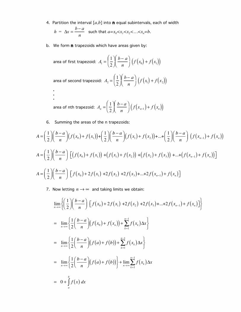
4. Partition the interval [a,b] into n equal subintervals, each of width

h = !x =b " a

n such that a=x0<x1<x2<…<xn=b.

b. We form n trapezoids which have areas given by:

area of first trapezoid:

A1

=1

2

!

" # $

%

b & a

n

!

" # $

% f x

0( ) + f x1( )( )

area of second trapezoid:

A2

=1

2

!

" # $

%

b & a

n

!

" # $

% f x

1( ) + f x2( )( )

.

.

.

area of nth trapezoid:

An =1

2

!

" # $

%

b & a

n

!

" # $

% f xn&1( ) + f xn( )( )

6. Summing the areas of the n trapezoids:

A =1

2

!"#

$%&b ' an

!"#

$%&f x

0( ) + f x1( )( )+

1

2

!"#

$%&b ' an

!"#

$%&f x

1( ) + f x2( )( )+...+

1

2

!"#

$%&b ' an

!"#

$%&

f xn'1( ) + f xn( )( )

A =1

2

!"#

$%&b ' an

!"#

$%&

f x0( ) + f x

1( )( ) + f x1( ) + f x

2( )( ) + f x2( ) + f x

3( )( ) +...+ f xn'1( ) + f xn( )( )() *+

A =1

2

!"#

$%&b ' an

!"#

$%&

f x0( ) + 2 f x

1( ) +2 f x2( ) +2 f x

3( )+...+2 f xn'1( ) + f xn( )() *+

7. Now letting n! " and taking limits we obtain:

limn!"

1

2

#$%

&'(b ) an

#$%

&'(

f x0( ) + 2 f x

1( ) +2 f x2( ) +2 f x

3( )+...+2 f xn)1( ) + f xn( )*+ ,-./0

123

= limn!"

1

2

b # an

$%&

'()f x

0( ) + f xn( )( ) + f xk( )*xk=1

n#1

+,-.

/01

= limn!"

1

2

b # an

$%&

'()f a( ) + f b( )( ) + f xk( )*x

k=1

n#1

+,-.

/01

= limn!"

1

2

b # an

$%&

'()f a( ) + f b( )( )

*+,

-./+ lim

n!"f xk( )0x

k=1

n#1

1

= 0 + f x( )a

b

! dx

B. Trapezoidal Rule

Let f be continuous on [a,b]. To approximate

f x( )a

b

! dx use

Tn =1

2

!"#

$%&b ' an

!"#

$%&

f x0( ) + 2 f x

1( ) +2 f x2( )+...+2 f xn'1( ) + f xn( )() *+

OR

Tn =,x2

!"#

$%&

f x0( ) + 2 f x

1( ) +2 f x2( )+...+2 f xn'1( ) + f xn( )() *+

where ,x =b ' an

and xi = a + i ,x( ).

**Note: the coefficients in the Trapezoidal Rule follow the pattern: 1 2 2…2 2 1

C. The Error Estimate for the Trapezoidal Rule , ET

1.

ET = f x( )a

b

! dx " Tn , where Tn is the Trapezoidal Rule.

2. If ! ! f is continuous and K is any upper bound for the values of

! ! f on [a,b],

then

ET!

b - a

12

"

# $ %

& 'x( )

2

K =b - a( )

3

12n2

"

#

$

%

&

( K , where

!x =b - a

n

D. Examples

1a. Use the Trapezoidal Rule to estimate x4+ x( )

1

2

1

! dx using n=4.

1b. Find the error in the trapezoidal approximation, | ET.|. 1c. Find an upper bound for | ET.|.

1d. How large do we have to choose n so that the approximation Tn to the integral in

(a) is accurate to 0.001?

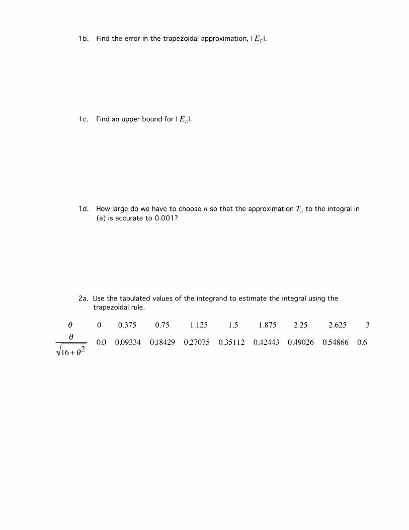
2a. Use the tabulated values of the integrand to estimate the integral using the trapezoidal rule.

! 0 0.375 0.75 1.125 1.5 1.875 2.25 2.625 3

!

16 +!2

0.0 0.09334 0.18429 0.27075 0.35112 0.42443 0.49026 0.54866 0.6

2b. Find the error in the trapezoidal approximation, | ET.|.

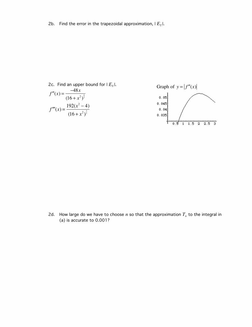
2c. Find an upper bound for | ET.|.

!!f (x) ="48x

(16 + x2)52

!!!f (x) =192(x

2" 4)

(16 + x2)72

2d. How large do we have to choose n so that the approximation Tn to the integral in

(a) is accurate to 0.001?

Graph of y = !!f (x)

I I I. Simpson’s / Parabolic Rule A. Development of Formula

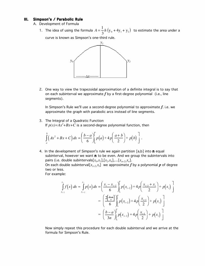
1. The idea of using the formula A =1

3h y0 + 4y1 + y2( ) to estimate the area under a

curve is known as Simpson’s one-third rule.

2. One way to view the trapezoidal approximation of a definite integral is to say that

on each subinterval we approximate f by a first-degree polynomial (i.e., line segments).

In Simpson's Rule we'll use a second-degree polynomial to approximate f. i.e. we approximate the graph with parabolic arcs instead of line segments.

3. The Integral of a Quadratic Function

If p(x)=Ax2+Bx+C is a second-degree polynomial function, then

Ax2

+ Bx + C( )a

b

! dx =b " a

6

#

$ % &

' p a( ) + 4 p

a + b

2

#

$ % &

' + p b( )

(

) *

+

, - .

4. In the development of Simpson's rule we again partition [a,b] into n equal

subinterval, however we want n to be even. And we group the subintervals into pairs (i.e. double subintervals[x0,x2],[x2,x4],…[x(n-2),xn]. On each double subinterval[x(i-2),xI] we approximate f by a polynomial p of degree two or less. For example:

f x( )xi!2

x i

" dx # p x( )x i!2

x i

" dx =xi ! xi!2

6

$

% & '

( p xi!2( ) + 4 p

xi!2+ xi

2

$

% & '

( + p xi( )

)

* +

,

- .

= 2 b! a

n[ ]6

$

% &

'

( / p xi!2( ) + 4 p

xi!1

2

$

% & '

( + p xi( )

)

* +

,

- .

= b ! a

3n

$

% & '

( p xi! 2( ) + 4 p

xi!1

2

$

% & '

( + p xi( )

)

* +

,

- .

Now simply repeat this procedure for each double subinterval and we arrive at the formula for Simpson's Rule.

-------Δx--------

y0 y2

y1

B. Simpson's Rule (n is even)

Let f be continuous on [a,b]. Simpson's Rule for approximating

f x( )a

b

! dx is given by

S = b ! a

3n

"

# $ %

& f x

0( ) + 4 f x1( ) + 2 f x

2( ) + 4 f x3( ) +... + 4 f xn!1( ) + f xn( ) [ ]

OR

S = 'x

3

"

# $ %

& f x

0( ) + 4 f x1( ) + 2 f x

2( ) + 4 f x3( ) +... + 4 f xn!1( ) + f xn( ) [ ]

where 'x =b ! a

n .

Note: the coefficients in Simpson's Rule follow the pattern: 1 4 2 4 2 4 ... 4 2 4 1

B. The Error Estimate for Simpson's Rule, ES

1.

ES = f x( )a

b

! dx " Sn where Sn is Simpson’s Rule.

2. If f

4( ) is continuous and K is any upper bound for the values of

f4( ) on [a,b],

then

ES!

b - a

180

"

# $ %

& 'x( )

4

K =b - a( )

5

180n4

"

#

$

%

&

( K , where

!x =b - a

n

C. Examples

1a. Use the Simpson's Rule to estimate x4+ x( )

1

2

1

! dx using n=4.

b. Find the error in the Simpson’s approximation, | ES.|.

c. Find an upper bound for | ES.|. d. How large do we have to choose n so that the approximation Sn to the integral

in (a) is accurate to 0.0001?

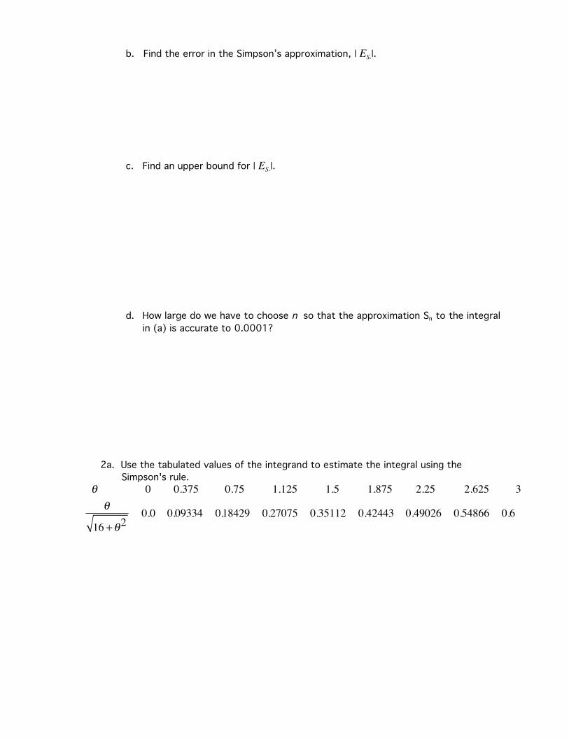
2a. Use the tabulated values of the integrand to estimate the integral using the Simpson's rule.

! 0 0.375 0.75 1.125 1.5 1.875 2.25 2.625 3

!

16 +!2

0.0 0.09334 0.18429 0.27075 0.35112 0.42443 0.49026 0.54866 0.6

b. Find the error in the Simpson's approximation, | ES.|.

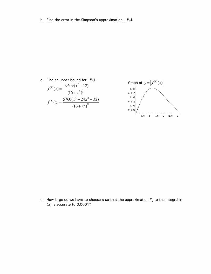
c. Find an upper bound for | ES.|.

f(4 )(x) =

!960x(x2!12)

(16 + x2)92

f(5)(x) =

5760(x4! 24x

2+ 32)

(16 + x2)112

d. How large do we have to choose n so that the approximation Sn to the integral in (a) is accurate to 0.0001?

Graph of y = f(4 )(x)

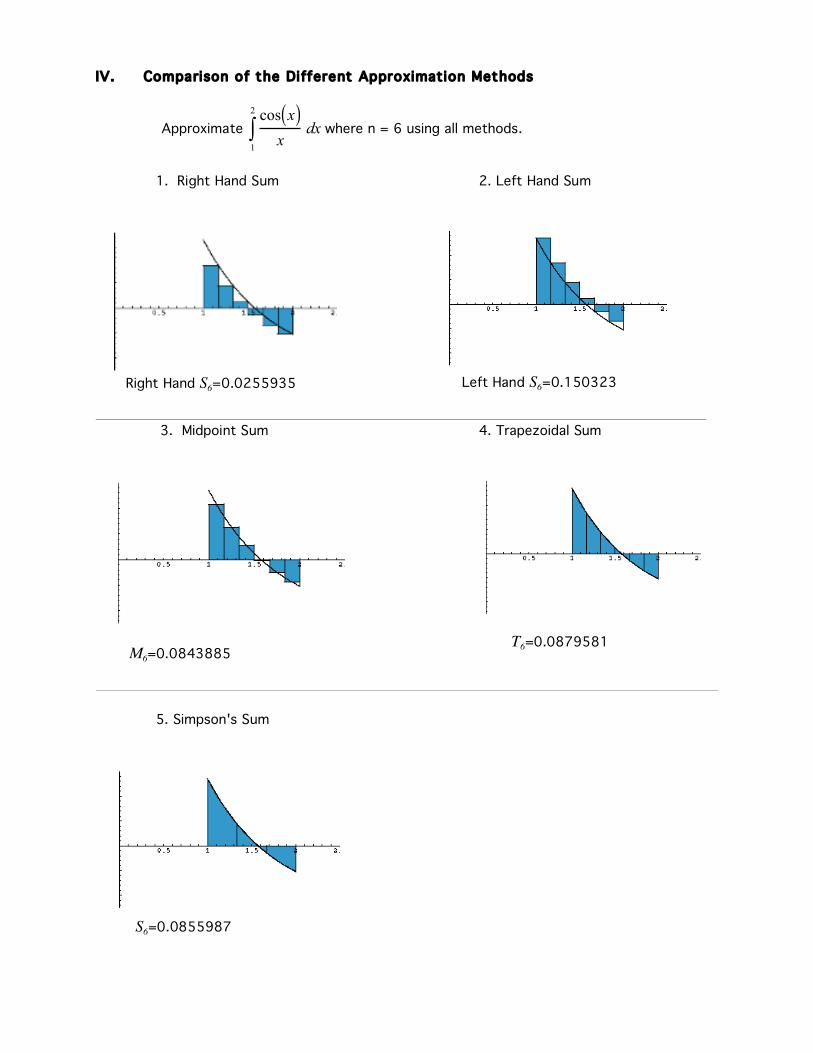
IV. Comparison of the Different Approximation Methods

Approximate

cos x( )x

dx

1

2

! where n = 6 using all methods.

1. Right Hand Sum 2. Left Hand Sum

3. Midpoint Sum 4. Trapezoidal Sum

5. Simpson's Sum

Right Hand S6=0.0255935 Left Hand S6=0.150323

M6=0.0843885 T6=0.0879581

S6=0.0855987