simulations - 2

J A Sellwood

Structure of an N-body code

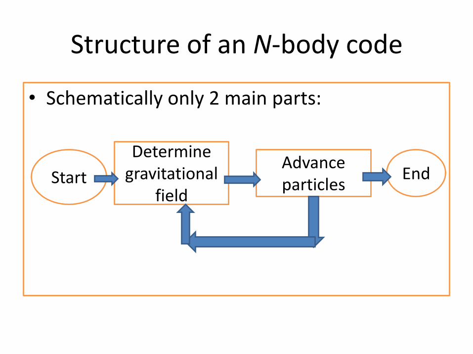
• Schematically only 2 main parts:

Determine gravitational

field

Advance particles Start End

• and are related through Poisson’s eq:

which is a 2nd order, elliptic PDE. Solutions require boundary conditions that are unknown for a isolated mass distribution

• So almost all methods start from the Poisson integral instead, which is a convolution

of with the spherically symmetric kernel P()

Solving for the gravitational field

Grids

• By far the most efficient methods to solve for the gravitational field use grids

– Cartesian, cylindrical polar, or spherical

– polar grids have additional advantages

• I will describe some of the dangers of using these methods

– but they can all be avoided with care

Cartesian grids

• For simplicity, focus on the solution for in 1D:

(j) = k w(k) P(|xk-xj|)

• which is a convolution of the symmetric kernel P with the masses w

• Convolutions reduce to multiplications in Fourier space and FFTs are fast and efficient

• Sounds easy, but there are pitfalls

Grid doubling • Potential kernel (black)

should be 2 grid width

– 3 source masses

• Fourier transformation implicitly introduces periodic images

• Their effect has to be excluded

• Solution is to double grid in each dimension

3D Cartesian grids

• In 3D, the grid needs to be 8 times larger than the active region – which is wasteful

• James (1977) reverted to Poisson’s equation for and devised a clever method to determine the boundary potential

• His method is about twice as fast as the grid doubling method

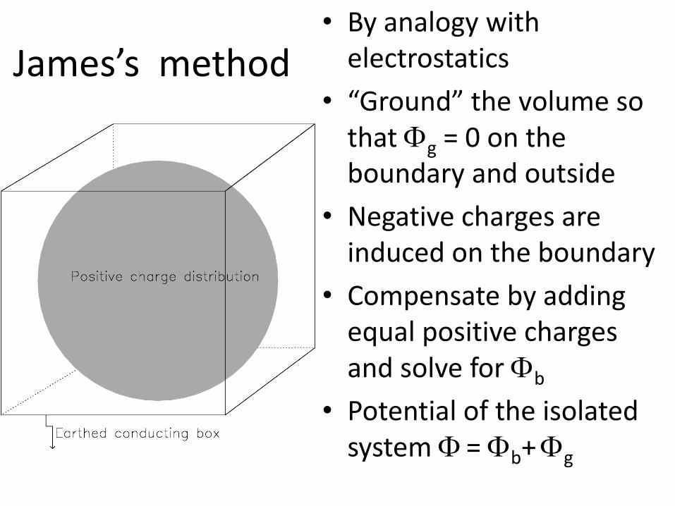
James’s method • By analogy with

electrostatics

• “Ground” the volume so that g = 0 on the boundary and outside

• Negative charges are induced on the boundary

• Compensate by adding equal positive charges and solve for b

• Potential of the isolated system = b+ g

Adaptive grids

• Uniformly-spaced Cartesian grids are unsuitable for inhomogeneous galaxies

• Adaptive refinement better (e.g. Kravtsov et al. 1997, Knebe et al. 2001)

• Grid cells can be divided hierarchically to yield more highly resolved forces where the density is greater

– stop dividing while still many particles per cell

• Also need shorter time steps where this is done, since accelerations are stronger

• The acceleration a = -.

• If we have calculated at all grid points (i,j,k) then the simplest estimate is

• But this has the disadvantages

1. degrades resolution – average over 2hx

2. is not easily accomplished near grid edges, and

3. is numerically challenging on non-Cartesian grids

Acceleration components

Acceleration components

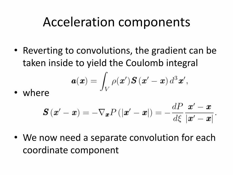
• Reverting to convolutions, the gradient can be taken inside to yield the Coulomb integral

• where

• We now need a separate convolution for each coordinate component

Advantages

• The extra computational cost of convolving for the accelerations is outweighed by 2 major advantages

1) we do not need to estimate slopes by differencing values of between grid points avoids all the difficulties

2) The acceleration experienced by a particle is less dependent on its sub-cell position i.e. grid noise is reduced

Interpolation

• Particles move continuously through the volume, but at each time step

1. distribute the mass of a particle over the surrounding grid points

2. interpolate between the forces determined at the grid points to find the force acting on each particle

• Many possible schemes

– weights for step 1 must be the same as step 2 else the particle will accelerate itself!

Linear interpolation

• Fast and adequate

• Illustrate in 2D

• Forces between any pair of particles are equal and opposite

• but may not be perfectly co-linear

– exaggerated in the figure

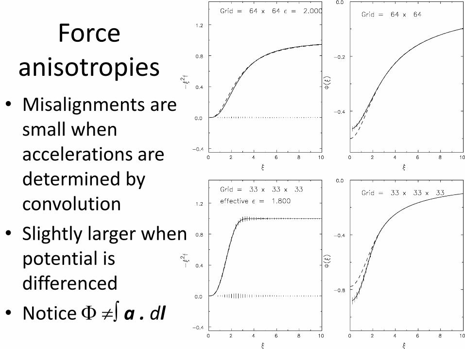
Force anisotropies

• Misalignments are small when accelerations are determined by convolution

• Slightly larger when potential is differenced

• Notice a . dl

Polar grids

• Two significant advantages – More natural grid shape for disk galaxies

– Higher spatial resolution in the dense center

• Forces from a convolution – Mass is periodic in azimuth, so FFTs (without grid

doubling) are ideal

wm = w(j) e2ijm/M

where m is the sectoral harmonic

– Radial part requires direct convolution

– In 3D the grid has to be doubled in the vertical direction

Forces on a polar grid

• Interparticle forces can be acceptably close to those between softened point masses

• But a major advantage of polar grids is that forces can be smoothed by filtering out the high m terms

– density fluctuations with high angular periodicities contain no meaningful information and the gravitational field need reflect only low-m variations

• i.e. the mass of each particle is smeared in azimuth

Spherical grid

• The potential at a field point r of a point mass M at r can be expanded in surface harmonics, Ylm(,)

where r (r) is the lesser (greater) of r and r

• This expression can be used in N-body codes that are ideal for nearly spherical systems (Villumsen 1982,

van Albada 1982, White 1983, McGlynn 1984, etc.)

• I use a grid, else particles must be sorted in r

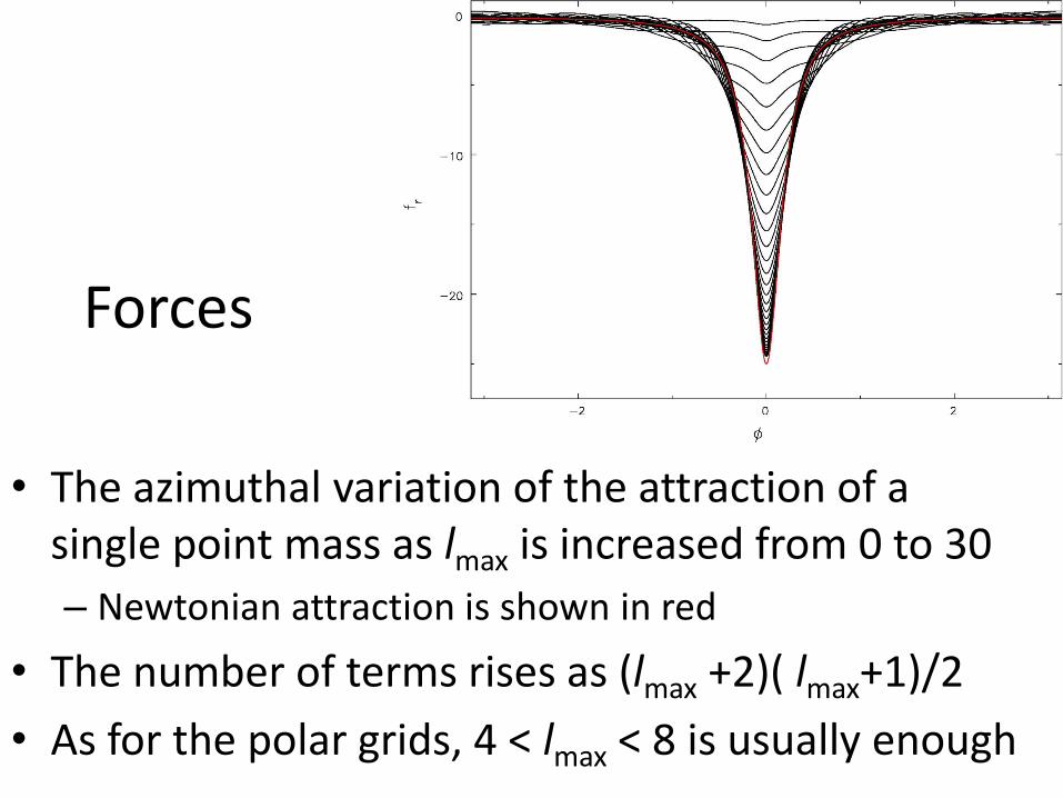
Forces

• The azimuthal variation of the attraction of a single point mass as lmax is increased from 0 to 30

– Newtonian attraction is shown in red

• The number of terms rises as (lmax +2)( lmax+1)/2

• As for the polar grids, 4 < lmax < 8 is usually enough

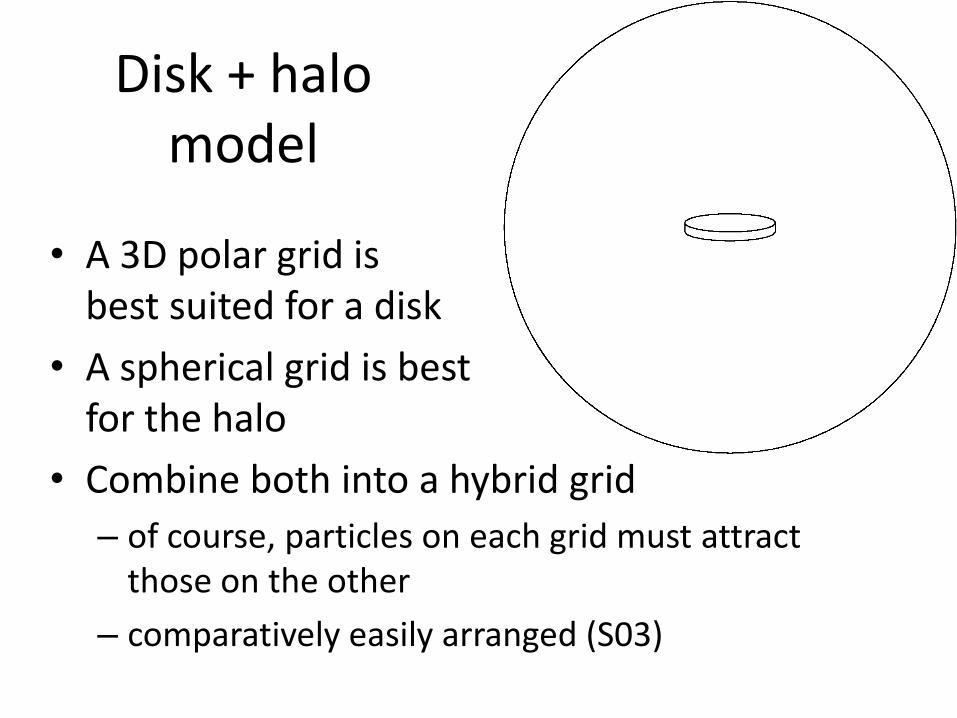
Disk + halo model

• A 3D polar grid is best suited for a disk

• A spherical grid is best for the halo

• Combine both into a hybrid grid

– of course, particles on each grid must attract those on the other

– comparatively easily arranged (S03)

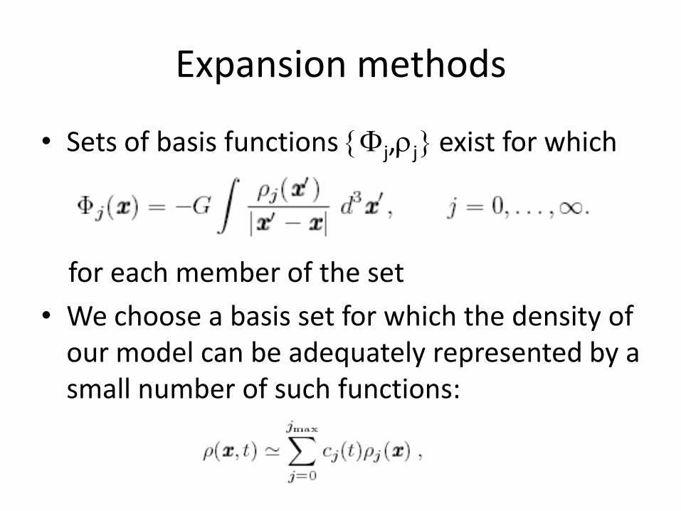
Expansion methods

• Sets of basis functions j,j exist for which

for each member of the set

• We choose a basis set for which the density of our model can be adequately represented by a small number of such functions:

Expansion methods (contd)

• The accelerations for each particle are then

• The coefficients for the expansion are

where M and R0 are suitable scaling factors

• These 2 equations are all you need!

Applications

• The expansion method is highly efficient when jmax is small and it is very easily parallelized. As a result, it has been widely discussed – (Clutton-Brock 1972; Hernquist & Ostriker 1992; Saha 1993;

Earn & Sellwood 1995; Weinberg 1999; etc.)

• However, it is inflexible: an evolving mass distribution may no longer be a good match to the basis – compensating by increasing jmax is costly and rarely adequate.

• It is useful only for near equilibrium models

Tree codes

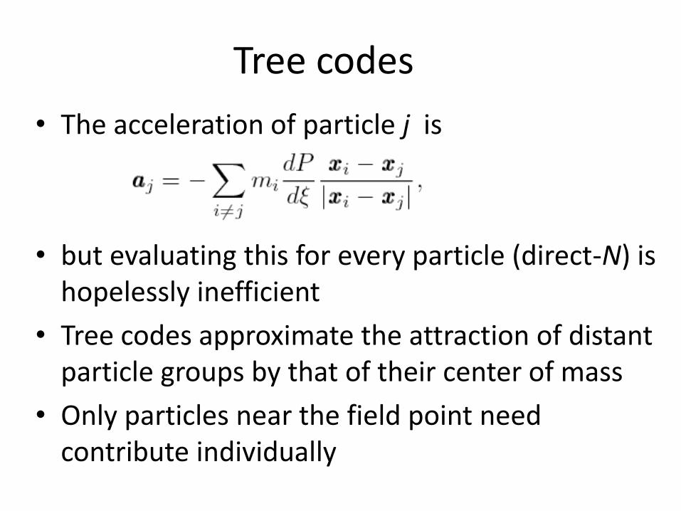
• The acceleration of particle j is

• but evaluating this for every particle (direct-N) is hopelessly inefficient

• Tree codes approximate the attraction of distant particle groups by that of their center of mass

• Only particles near the field point need contribute individually

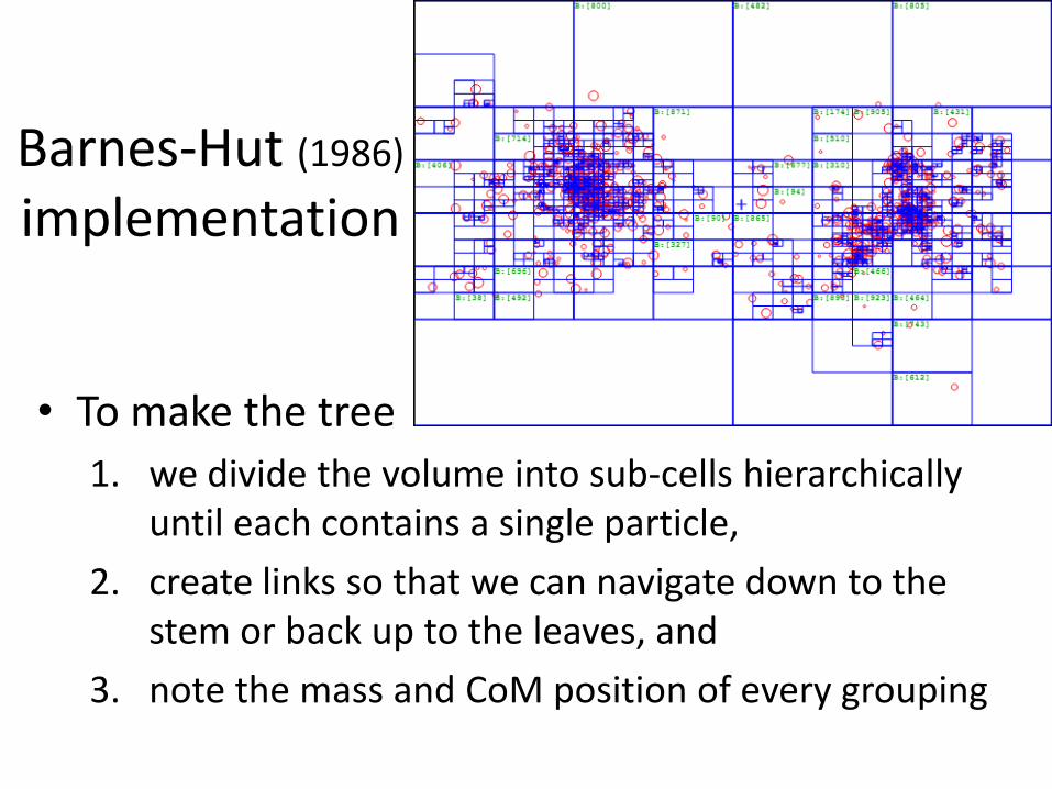
Barnes-Hut (1986)

implementation

• To make the tree

1. we divide the volume into sub-cells hierarchically until each contains a single particle,

2. create links so that we can navigate down to the stem or back up to the leaves, and

3. note the mass and CoM position of every grouping

Using the tree

• For each particle

1. start at the stem of the tree

2. find distance d to the CoM of the grouping in a box of width L

3. if L > d max then we must ascend the tree to the next level and go back to step 2

4. otherwise, the attraction of the group is –Gmg/d2

• The opening angle max is a key parameter

– generally max 0.7 seems adequate

Multipoles

• Some prefer to compute higher multipoles for each grouping

– allows larger opening angles so that fewer groupings need to be opened

• Saving the position of the CoM, and not just the box center, eliminates the dipole term

Advantages and disadvantages

• Advantages

1. Tree codes are immediately applicable to systems of arbitrary shape

2. They are inherently adaptive – high resolution in regions of high density

3. Generally easy to use

• Disadvantages

1. They are a few 10 - 100 times slower than grid methods for the same N on a single processor

2. Harder to parallelize

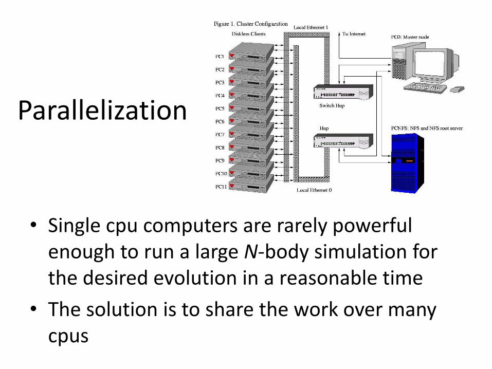
Parallelization

• Single cpu computers are rarely powerful enough to run a large N-body simulation for the desired evolution in a reasonable time

• The solution is to share the work over many cpus

Sharing the work

• Transferring information between cpus is slow

• But we must ensure that all particles experience the gravitational field due to all other particles

• Not so difficult for grids:

– divide the particles in the simulation between cpus

– assign the masses to a local copy of the grid

– combine the masses on the different grids

– share the work of computing the field

• e.g. one grid plane for each cpu

– combine the results and distribute them

Parallelizing tree codes

• Much more difficult

– the tree inherently includes all particles

– pieces of the tree, and their associated particles can be assigned to each node

– advancing the particles requires forces from other nodes

– in collapses, for example, some parts of the tree become much larger than others - may need to “rebalance” the load on each cpu

Which method is best?

• Criterion?

– more or less collisional – almost no difference

• Fastest?

– high premium on using the largest N

• Most adaptable?

– SFP methods are too inflexible

– Tree methods are most versatile, but an extravagance for problems that could be done on a grid

– choose your grid to match the geometry