Hamiltonian Method in the

Braneworld

Neven Bilić

Ruđer Bošković Institute

Zagreb

Legendere Transformation

Basic Thermodynamics and fluid Mechanics

Lagrangian and Hamiltonian

Basic Cosmology

Lecture 1 – Preliminaries

Lecture 2 – Braneworld

Universe

Strings and Branes

Randal Sundrum Model

Braneworld Cosmology

AdS/CFT and Braneworld Holography

Lecture 3 – Applications

Quintessence and K-essence

DE/DM unification

Tachyon condensate in a Braneworld

Lecture 1 - Preliminaries

Legendre Transformation

Consider an arbitrary smooth function f(x). We can define another

function g(u) such that

where the variables x and y (called conjugate variables) are related via

,f g

y xx u

(1)

Proof:

At an arbitrary point x0 the function f(x) can be locally represented by

where 0

0

x

fu

x0 0 0( )f x u x g

( ) ( )f x g u xu

g depends on u0

0 tanuf

x -g x0

By the symmetry of (1) we can also write

0

0

u

gx

uwhere

Exercise No 1: Prove this using the geometry in the figure

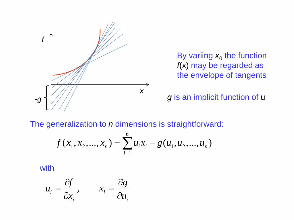
Simple geometric meaning

0 0 0( )g u x u f

f

x

By variing x0 the function

f(x) may be regarded as

the envelope of tangents

The generalization to n dimensions is straightforward:

with

-g g is an implicit function of u

,i i

i i

f gu x

x u

1 2 1 2

1

( , ,..., ) ( , ,..., )n

n i i n

i

f x x x u x g u u u

Applications

1) Classical mechanics

( ) = ( )i j j i

j

p q p qH L ,i i

i i

p qq p

L H

2) Thermodynamics

( , ) = ( , )F T V E S V TS ,F E

S TT S

F – Helmholz free energy, E – internal energy, S – entropy

1) Quantum firld theory

[ ] = [ ] ( ) ( )W J dxJ x x ( ) , ( )( ) ( )

WJ x x

x J x

W – generating functional of connected Green’s functions

Γ – generating functional of 1-particle irreducible Green’s functions

Basic Thermodynamics

We will distinguish the grandcanonical from canonical ensemble

The conjugate variables:

V – volume p – pressure

S – entropy T – temperature

N – particle number μ – chemical potential

Canonical: particle number N fixed. Related potentials are

the Gibbs free energy G and internal energy E

Grandcanonical: chemical potential μ fixed. N is not conserved.

Related potentials are the grandcanonical thermodynamic potential

Ω=-pV and internal energy E

Canonical ensemble

( , ) ( , )G T p E S V TS pV

The Gibbs free energy G is related to the internal energy E via

Legendre transformation

The well known thermodynamic identities follow:

together with the conditions

, ,G G

S VT p

,E E

T pS V

(2)

(3)

dE TdS pdV

Exercise No 2: Derive (4) and (5) from (2) and (3)

(4)

dG SdT Vdp (5)

TDS equation

Canonical ensemble

The potentials G and E are related the Helmholz free energy F

via respective Legendre transformation,

( , ) ( , )F T V G T p pV

So that Fp

V

( , ) = ( , )F T V E S V TS

FS

T

Grandcanonical ensemble

( , ) ( , )T E S N TS N

The grandcanonical thermodynamic potential Ω=-pV is related to the

internal energy E=ρV , entropy S=sV and particle number N=nV via

Legendre transformation

which may be expressed locally (dividing by V )

together with the conditions

, ,p p

s nT

(6)

(7)

( , ) ( , )p T Ts n s n

,Ts n

1pd nd d

T T T

Two useful thermodynamic identities follow

Gibbs-Duhem relation

1sdw Td dp

n n

Exercise No 3: Derive (9) and (10) from (6)-(8)

(9)

(10)

pw

n

Introducing the specific enthalpy (or the specific heat content)

(8)

TDS equation

We will assume that matter is a perfect fluid

described by the energy-momentum tensor

u – fluid velocity

T – energy-momentum tensor

p – pressure

ρ – energy density

( )T p u u pg

Basic Fluid Mechanics

0=;T

0=;Tu

0,=)(3 pH

0)( , uppup

,=,=,=,=3 ;,,; uuupupuuH

The energy momentum conservation

yields, as its longitudinal part , the continuity equation

and, as its transverse part, the Euler equation

where

H – expansion (Hubble expansion rate in cosmology)

Exercise No 4: Derive (11) and (12)

(11)

(12)

Velocity field

It is convenient to parameterize the four-velocity uμ in terms of three-

velocity components. To do this, we use the projection operator

g t t

where tμ is the time translation unit vector . We split up

the vector uμ in two parts: one parallel with and the other orthogonal to tμ : 0 00t g g

( ) ,u t g t t u t u

yielding

where

Exercise No 5: Derive (13)

(13)

Isentropic and adiabatic fluid

A flow is said to be isentropic when the specific entropy s/n is constant,

i.e., when

and is said to be adiabatic when s/n is constant along the flow lines,

i.e., when

As a consequence of (14) and the thermodynamic identity (8)

(TdS equation) the Euler equation (12) simplifies to

(14)

In this case, we may introduce a scalar function φ such that

(15)

(16)

Exercise No 6: Derive (15) from (12) and (14)

which obviously solves (15)

,wu

,wuNB1: The solution (16) is the relativistic analogue of potential

flow in nonrelativistic fluid dynamics

L.D. Landau, E.M. Lifshitz, Fluid Mechanics, Pergamon, Oxford,1993.

NB2: The potential flow (16) implies the isentropic Euler equation (15) but

not the other way round. However if the fluid is isentropic and

irrotational, then equations (15) and (16) are equivalent. The fluid is said

to be irrotational if its vorticity vanishes. The vorticity is defined as

where

Vanishing vorticity, i.e., ωμν=0, implies

This equation is satisfied if and only if and the Euler equation

(15) is satisfied identically ,wu

A.H. Taub, Relativistic Fluid Mechanics, Ann. Rev. Fluid Mech. 10 (1978) 301

The dream of all physicists is a comprehensive

fundamental theory, which is often in popular scientific

literature called the ‘’theory of everything’’. Of course,

nobody expects that this theory provides answers to all

the issues, for example, the cause of a cancer, how the

mind works, and so on. From the theory of everything

we only require to explain basic processes in nature.

Today most physicists share the following view of the

world: the laws of nature are unambiguously described

by the principle of some unique action (or Lagrangian)

that fully defines the vacuum, the spectrum of elementary

particles, forces and symmetries.

Lagrangian and Hamiltonian

The principle of least action

yields classical equations of motion

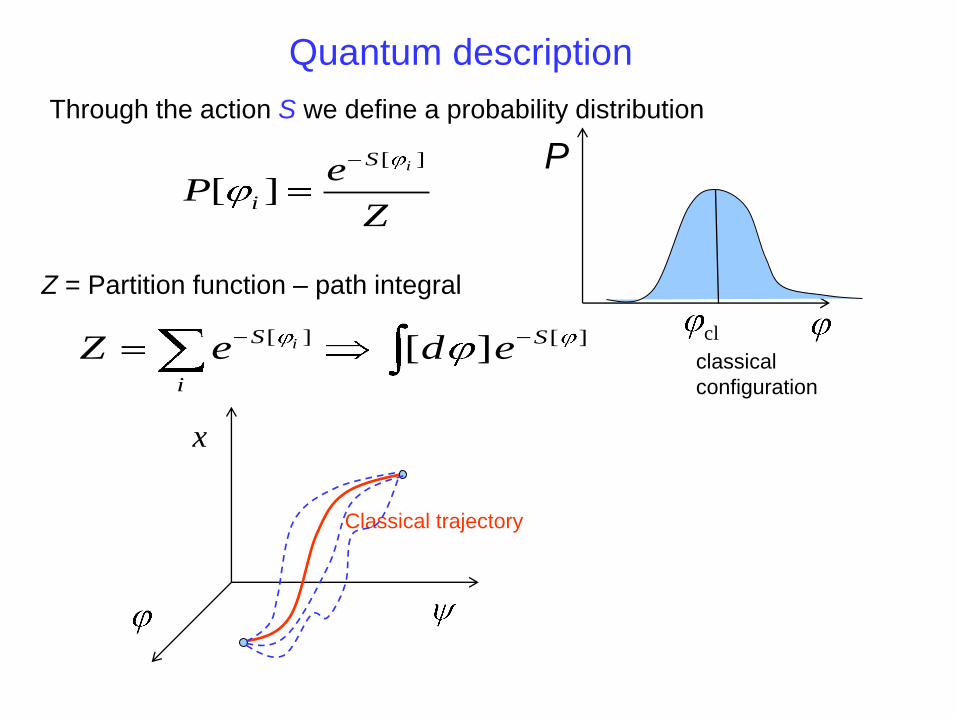
Classical trajectory

Classical description

1

x

2

1 2, ,

S

cl

classical

configuration

stable

metastable

4 det ( , )S d x g XL, ,X g

One can easily generalize this to more fields

with

Consider a single selfinteracting scalar field θ with with a general

action

where

0S

, ,i i iX g

[ ] [ ][ ]iS S

i

Z e d e

Quantum description

Through the action S we define a probability distribution

P

classical

configuration

Classical trajectory

x

Z = Partition function – path integral

cl

[ ]

[ ]iS

i

eP

Z

From the requirement δS=0 one finds the classical equations of motion

If L does not depend on θi, the associated current is conserved, i.e.

( ) ,ii X iJ = L

To each scalar field θi one can associate a current

where

( ); 0iJ

This current conservation law follows immediately from (17) and is

related to the shift symmetry

i i c

(17) , ;i i

L L

The canonical Hamiltonian is defined through the usual Legendre

transformation that involves the conjugate variables θ,0 and π0

0 0

can , ,0 ,0 ,( , , ) = ( , , ), 1,2,3i i iH L

where

We shall use a covariant definition (de Donder-Weyl Hamiltonian)

, ,( , ) = ( , )H L

,

,

= =L H

where

(18)

(19)

0 can,0 0

,0

= =L H

Hamiltonian

Historically, the covariant Hamiltonian was first introduced by De Donder

1930 and Weyl 1935 in the so called polysymplectic formalizm

Th. De Donder, Th´eorie Invariantive Du Calcul des Variations, Gaultier-

Villars & Cia., Paris, France (1930).

H. Weyl, Annals of Mathematics 36, 607 (1935)

Recent references

C. Cremaschini and M.Tessarotto, ``Manifest Covariant Hamiltonian Theory of

General Relativity,'‘ Appl. Phys. Res. 8, 60 (2016), arXiv:1609.04422

J. Struckmeier, A. Redelbach, Covariant Hamiltonian Field Theory, Int. J. Mod.

Phys. E17: 435-491, 2008, arXiv:0811.0508

It may be easily shown that the covariant definition of H coincides with

the energy density ρ in the field theoretical description of a perfect

relativistic fluid which we will discuss shortly

Examples:

1( )

2X VL

( )

1

U

XH

1) The standard scalar field Lagrangian

2) The Born-Infeld (tachyon) Lagrangian

( ) 1U XL

1( )

2X VH

( )T p u u pg

, ,

22

detX

ST g

ggL L

, ,X g

Field theoretical description of a fluid

This may be written in a perfect fluid form provided X>0

we define the energy momentum tensor

p L 2 XXL L

where

where we identify the velocity, pressure and energy density

XX

LLwhere

Using a general single field Lagrangian

,u

X

Exercise No 7: Prove ρ = H

4 det ( , )S d x g XL

Suppose for definitness that L depends on two fields Θ and Φ and

and their respective kinetic terms and

We introduce the canonical conjugate momentum fields

, ,

, ,

= 2 = 2Y Yg gL L

L L

For timelike and we may also define the norms

= =g g

We shall assume that the dependence on kinetic terms can be separated,

i.e., that the Lagrangian can be expressed as

1 2( , , , ) = ( , , ) ( , , )X Y X YL L L

,,

Hamilton field equations

, ,X g , ,Y g

(20)

The corresponding energy momentum tensor

may be expressed as a sum of two perfect fluids

1 1 1 1 2 2 2 2 1 2= ( ) ( ) ( )T p u u p u u p p g

with

(1) (1) (2) (2)= 2 2 2X YT g g gg

LL L L L L

1 2= =u u

(2) (2) (2)

2 2= = 2Y Yp YL L L

(1) (1) (1)

1 1= = 2X Xp XL L L

It may be easily verified that the Hamiltonian equals to

the total energy density

1 2= 3 =TH L

, , , ,( , , , ) = ( , , , )H L

The field variables are constrained by

H is related to L through the Legendre transformation

, ,

, ,

= =

= =

H H

L L

(21)

(22)

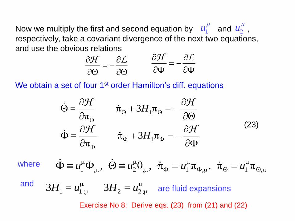
Now we multiply the first and second equation by and ,

respectively, take a covariant divergence of the next two equations,

and use the obvious relations

2u1u

1= 3HH H

1= 3HH H

H LH L

We obtain a set of four 1st order Hamilton’s diff. equations

where 1 , 2 , 1 , 1 ,, , ,u u u u

1 1 ; 2 2 ;3 = 3 =H u H u are fluid expansions and

Exercise No 8: Derive eqs. (23) from (21) and (22)

(23)

• General relativity – gravity

G = T

Matter determines the space-time geometry

Geometry determines the motion of matter

• Homogeneity and isotropy of space – approximate

property on very large scales (~Glyrs today)

• Fluctuations of matter and geometry in the early

Universe cause structure formation (stars, galaxies,

clusters ...)

Basic Cosmology

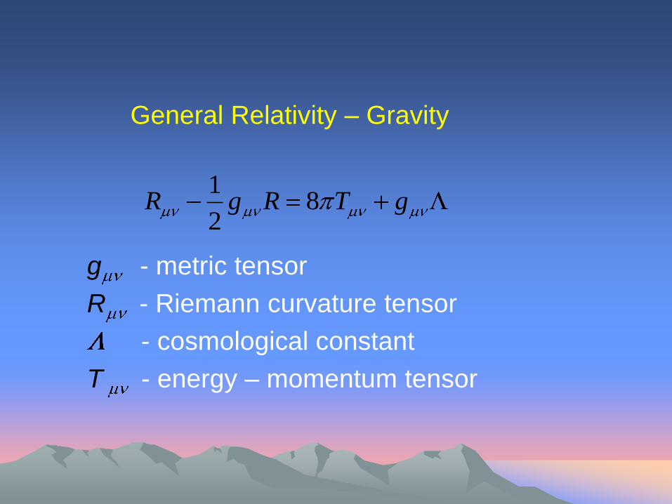
General Relativity – Gravity

g - metric tensor

R - Riemann curvature tensor

- cosmological constant

T - energy – momentum tensor

18

2R g R T g

Homogeneity and isotropy of space

22 2 2 2 2

2( )

1

drds dt a t r d

kr

Cosmological principle

the curvature constant k takes on the values 1, 0, or -1,

for a closed, flat, or open universe, respectively.

– cosmological scale ( )a t

• radiation

• dust

• vacuum

4( 3 )

3

Ga p

; 0T3(1 )wa w p

Various kinds of cosmic fluids with different w

4

R R 3 1 3p w a3

M 0 0p w a

k

0 open

0 flat

0 closed

Friedman equations

01p w a

2

2

8

3

a k G

a a

expansion ratea

Ha

Density of Matter in Space

The best agreement with cosmologic

observations are obtained by the models with a

flat space

According to Einstein’s theory, a flat space

universe requires critical matter density cr today

cr 10-29 g/cm3

Ω= / cr ratio of the actual to the critical density

For a flat space Ω=1

From astronomical

observations:

luminous matter (stars,

galaxies, gas ...)

lum/ cr 0.5%

From the light element

abundances and comparison

with the Big Bang

nucleosynthesis:

baryonic matter(protons,

neutrons, nuclei) Bar/ cr 5%

Total matter density fraction ΩM= M/ cr 0.31

Accelerated expansion and comparison of the standard Big Bang model with observations requires that the dark energy density (vacuum energy) today ΩΛ= / cr = 0. 69%

What does the Universe consist of?

DMDM

tot tot tot

0.05 0.26 0.69BB

These fractions change with time but for a

spatially flat Universe the following always holds:

Density fractions of various kinds of matter today with

respect to the total density

tot crit

3 4 1/2

0( ) ( )M RH a H a a

Easy to calculate using the present observed fractions of

matter, radiation and vacuum energy.

For a spatially flat Universe from the first Friedmann

equation and energy conservation we have

2 1

0 100Gpc/s (14.5942Gyr) , 0.67H h h

The age of the Universe T can be calculated using

Age of the Universe

Exercise No 9: Calculate T using

ΩΛ=0.69, ΩM=0.31, ΩR=0.

1

0 0

Tda

T dtaH

0.69

0.24

0.04

0.01

Dark nature of the Universe – Dark Matter

According to present recent observations (Planck Satellite Mission):

• Out of that less then 5% is ordinary (“baryonic”)

• About 24% is Dark Matter

• About 69% is Dark Energy (Vacuum Energy)

More than 99% of matter is not luminous

Hot DM refers to low-mass neutral particles that are still

relativistic when galaxy-size masses ( ) are first

encompassed within the horizon. Hence, fluctuations on

galaxy scales are wiped out. Standard examples of hot

DM are neutrinos and majorons. They are still in

thermal equilibrium after the QCD deconfinement

transition, which took place at TQCD ≈ 150 MeV. Hot DM

particles have a cosmological number density

comparable with that of microwave background

photons, which implies an upper bound to their mass of

a few tens of eV.

M1210

Warm DM particles are just becoming nonrelativistic

when galaxy-size masses enter the horizon. Warm

DM particles interact much more weakly than

neutrinos. They decouple (i.e., their mean free path

first exceeds the horizon size) at T>>TQCD. As a

consequence, their mass is expected to be roughly

an order of magnitude larger, than hot DM particles.

Examples of warm DM are keV sterile neutrino,

axino, or gravitino in soft supersymmetry breaking

scenarios.

Cold DM particles are already nonrelativistic

when even globular cluster masses ( )

enter the horizon. Hence, their free path is of

no cosmological importance. In other words, all

cosmologically relevant fluctuations survive in

a universe dominated by cold DM. The two

main particle candidates for cold dark matter

are the lowest supersymmetric weakly

interacting massive particles (WIMPs) and the

axion.

M610

Because gravity acts as an attractive force

between astrophysical objects we expect that

the expansion of the Universe will slowly

decelerate.

However, recent observations indicate that the

Universe expansion began to accelerate since

about 5 billion years ago.

Repulsive gravity?

Dark Energy

New term: Dark Energy – fluid with negative

pressure - generalization of the concept of vacuum energy

Accelerated expansion 0

One possible explanation is the existence of a fluid

with negative pressure such that

and in the second Friedmann equation the universe

acceleration becomes positive

3 0p

a

cosmological constant vacuum energy density

with equation of state p=-ρ. Its negative pressure may

be responsible for accelerated expansion!

Problems with Λ

1) Fine tuning problem. The calculation of the vacuum energy

density in field theory of the Standard Model of particle

physics gives the value about 10120 times higher than the

value of Λ obtained from observations. One possible way out

is fine tuning: a rather unnatural assumption that all

interactions of the standard model of particle physics

somehow conspire to yield cancellation between various

large contributions to the vacuum energy resulting in a small

value of Λ , in agreement with observations

2) Coincidence problem. Why is this fine tuned value of Λ

such that DM and DE are comparable today, leaving one to

rely on anthropic arguments?

Another important property of DE is that its density does not

vary with time or very weakly depends on time. In contrast ,

the density of ordinary matter varies rapidly because of a

rapid volume expansion.

The rough picture is that in the early Universe when the

density of matter exceeded the density of DE the Universe

expansion was slowing down. In the course of evolution the

matter density decreases and when the DE density began to

dominate, the Universe began to accelerate.

Time dependence of the DE density

Most popular models of dark energy

• Cosmological constant – vacuum energy density.

Energy density does not vary with time.

• Quintessence – a scalar field with a canonical kinetic

term. Energy density varies with time.

• Phantom quintessence – a scalar field with a negative

kinetic term. Energy density varies with time.

• k-essence – a scalar field whose Lagrangian is a

general function of kinetic energy. Energy density varies

with time.

• Quartessence – a model of unifying of DE and DM.

Special subclass of k-essence. One of the popular

models is the so-called Chaplygin gas

Early Universe - Inflation

A short period of inflation follows – very rapid

expansion -

1025 times in 10-32 s.

Observations of the cosmic

microwave background radiation

(CMB) show that the Universe is

homogeneous and isotropic. The

problem arises because the

information about CMB radiation

arrive from distant regions of the

Universe which were not in a causal

contact at the moment when radiation

had been emitted – in contradiction

with the observational fact that the

measured temperature of radiation is

equal (up to the deviations of at most

about 10-5) in all directions of

observation.

The horizon problem.

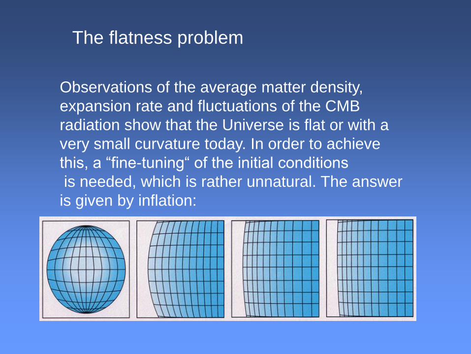
The flatness problem

Observations of the average matter density,

expansion rate and fluctuations of the CMB

radiation show that the Universe is flat or with a

very small curvature today. In order to achieve

this, a “fine-tuning“ of the initial conditions

is needed, which is rather unnatural. The answer

is given by inflation:

The initial density perturbations

The question is how the initial deviations from

homogeneity of the density are formed having in mind that

they should be about 10-5 in order to yield today’s

structures (stars, galaxies, clusters). The answer is given

by inflation: perturbations of density are created as

quantum fluctuations of the inflaton field.

510 510= ,v Hd

Measuring CMB; the temperature map of the sky.

KT 2.723=

KT 100=

KT 200=

Angular (multipole) spectrum of the fluctuations of the CMB

(Planck 2013)