braneworld cosmology beyond the low-energy limit
TRANSCRIPT

Braneworld Cosmology Beyond the
Low-energy Limit
Claudia de Rham
Girton College,
University of Cambridge
This dissertation is submitted for the degree of Doctor of Philosophy
August 2005

As I was walking up the stair,
I met a man who wasn’t there,
He wasn’t there again today,
I wish, I wish he’d stay away.
As I was sitting in my chair,
I knew the bottom wasn’t there,
Nor legs nor back, but I just sat,
Ignoring little things like that.
Hughes Mearns
i

ii

A Tosca,
Robin,
Palmitoa,
et vos Cousins,
for being there.
iii

iv

Declaration
This dissertation is my own work and contains nothing which is the outcome of work done
in collaboration with others, except as specified in the text and Acknowledgements.
I hereby declare that my thesis entitled:
Braneworld Cosmology Beyond the Low-energy Limit
is not substantially the same as any that I have submitted for a degree or diploma or
other qualification at any other University. I further state that no part of my thesis has
already been or is being concurrently submitted for any such degree, diploma or any other
qualification.
I further declare that this copy is identical in every respect to the soft-bound volume
examined for the Degree, expect that any alterations required by the Examiners have been
made.
Date: October 7, 2005
Signed:
Claudia de Rham Fernando Quevedo
v

vi

Acknowledgements
I would like to thank my supervisor, Anne Davis for all her support, motivation and advises
during the course of my PhD. Some special thanks to Sam Webster for very enjoyable
collaboration, to Joe Conlon, to Carsten van de Bruck for useful remarks, to Nick Manton
for comments on papers, and to Andrew Tolley for countless fruitful discussions, endless
enthusiasm and for comments on the manuscript. I would like to acknowledge as well
Girton College together with DAMTP and Cambridge University for financial support.
I specially wish to thank my family and in particular my parents for supporting my choices,
come what may, as well as Sophia, Mikael and Wayta for having been always present and
Inti. Marion Roman, Linda Uruchurtu Gomez, Gustavo Niz, Anna James and the students
of AIMS are all part of my best memories of my PhD course.
Pour finir, troll y a apporte une note speciale, et c’est a lui que je voudrais dedier ce dernier
merci.
vii

viii

Abstract
Advances in string/M-theory have recently motivated the study of braneworld scenarios for
which our Universe would be embedded in compactified extra dimensions. Playing the role
of a toy model, the five-dimensional Randall Sundrum scenario is of special interest. In that
model, the extra dimension is compactified on an S1/Z2 orbifold, with two three-branes on
the fixed point of the Z2 symmetry.
In this thesis, we develop a four-dimensional effective theory for Randall Sundrum mod-
els which allows us to calculate long wavelength adiabatic perturbations in a regime where
the ρ2 terms characteristic of braneworld cosmology are significant. This extends previous
work employing the moduli space approximation. We extend the treatment of the system to
include higher derivative corrections present in the context of braneworld cosmology. The
developed formalism allows us to study perturbations beyond the general long wavelength,
slow-velocity regime to which the usual moduli approximation is restricted. It enables us
to extend the study to a wide range of braneworld cosmology models for which the extra
terms play a significant role. As an example we discuss high energy inflation on the brane
and analyse the key observational features that distinguish braneworlds from ordinary in-
flation by considering scalar and tensor perturbations as well as non-gaussianities. We also
compare inflation and Cyclic models and study how they can be distinguished in terms of
these corrections.
We then focus on the study of the Randall Sundrum scenario in the case where the
boundary branes are very close. In that regime, we obtain an effective theory, correct to
all orders in brane velocity. The resulting theory is derived via recursive differentiations of
ix

the five-dimensional equations of motion. It extends the low-energy effective theory to the
high energy regime. In the case of cosmological symmetry the theory reproduces the five-
dimensional behaviour exactly, which the low-energy theory fails to do. This extension has
the remarkable property of including corrections only as powers of first order derivatives.
This important feature makes the theory particularly easy to solve. Perturbations in the
tensor and scalar sectors are then studied. When the branes are moving, the effective
Newtonian constant on the brane is shown to depend both on the separation of the branes
and on their velocity. In the small distance limit, we compute the exact dependence between
the four-dimensional and the five-dimensional Newtonian constants. We then extend the
theory by introducing a potential for the radion and show that for a fixed background,
the perturbations propagate the same way as they would in a standard four-dimensional
scenario.
x

Contents
1 Introduction 1
1.1 Early Universe Cosmology . . . . . . . . . . . . . . . . . . . . . . . . . . . 1
1.1.1 Cosmology . . . . . . . . . . . . . . . . . . . . . . . . . . . . . . . . 1
1.1.2 Early Universe and Modern Puzzles . . . . . . . . . . . . . . . . . . 3
1.1.3 Inflation . . . . . . . . . . . . . . . . . . . . . . . . . . . . . . . . . 7
1.2 Extra-dimensions and Braneworld . . . . . . . . . . . . . . . . . . . . . . . 12
1.2.1 Kaluza Klein Compactification and Extra Dimensions . . . . . . . . 12
1.2.2 Basic notions of String Theory . . . . . . . . . . . . . . . . . . . . . 14
1.2.3 M-theory and Orbifold Branes . . . . . . . . . . . . . . . . . . . . . 18
1.2.4 D-Branes as the End Points for Open Strings . . . . . . . . . . . . 20
1.2.5 Hierarchy Problem and Large Extra-dimensions . . . . . . . . . . . 22
1.3 Brane Gas and Dimensionality Puzzle . . . . . . . . . . . . . . . . . . . . . 24
1.3.1 Brane gas . . . . . . . . . . . . . . . . . . . . . . . . . . . . . . . . 25
1.3.2 String theory contributions to the dimensionality puzzle . . . . . . 28
1.4 Brane Inflation . . . . . . . . . . . . . . . . . . . . . . . . . . . . . . . . . 33
1.4.1 Dilaton and Moduli Fields . . . . . . . . . . . . . . . . . . . . . . . 33
1.4.2 D-brane Inflation . . . . . . . . . . . . . . . . . . . . . . . . . . . . 34
1.4.3 Brane - Antibrane Inflation . . . . . . . . . . . . . . . . . . . . . . 36
1.4.4 Inflation on a Probe D3-brane driven by a DBI Action . . . . . . . 38
1.4.5 Ekpyrotic Scenarios . . . . . . . . . . . . . . . . . . . . . . . . . . . 39
1.5 Outline . . . . . . . . . . . . . . . . . . . . . . . . . . . . . . . . . . . . . . 41
vii

CONTENTS
2 Braneworld Cosmology 45
2.1 Introduction . . . . . . . . . . . . . . . . . . . . . . . . . . . . . . . . . . . 45
2.2 Description of the Randall Sundrum model . . . . . . . . . . . . . . . . . . 47
2.3 Gauss-Codacci Formalism . . . . . . . . . . . . . . . . . . . . . . . . . . . 48
2.3.1 Derivation of the Gauss-Codacci Equations . . . . . . . . . . . . . . 48
2.3.2 Gauss-Codacci Equations on the Boundary Branes . . . . . . . . . 52
2.4 Background Behaviour . . . . . . . . . . . . . . . . . . . . . . . . . . . . . 53
2.5 Evolution of the Weyl Tensor . . . . . . . . . . . . . . . . . . . . . . . . . 56
2.6 Low-energy Effective Theory and Four-dimensional Action . . . . . . . . . 57
2.6.1 Low-energy Regime . . . . . . . . . . . . . . . . . . . . . . . . . . . 57
2.6.2 Leading Order . . . . . . . . . . . . . . . . . . . . . . . . . . . . . . 58
2.6.3 Expression for the Weyl Tensor . . . . . . . . . . . . . . . . . . . . 59
2.6.4 Background Behaviour . . . . . . . . . . . . . . . . . . . . . . . . . 61
2.6.5 Einstein Frame . . . . . . . . . . . . . . . . . . . . . . . . . . . . . 61
2.7 Kaluza Klein modes for Static Branes . . . . . . . . . . . . . . . . . . . . . 62
2.7.1 Derivative Expansion . . . . . . . . . . . . . . . . . . . . . . . . . . 62
2.7.2 Kaluza Klein Correction Outside a Source in Real Space . . . . . . 66
2.8 Extensions . . . . . . . . . . . . . . . . . . . . . . . . . . . . . . . . . . . . 67
2.8.1 Bulk Scalar Field and Potential for the Radion . . . . . . . . . . . . 67
2.8.2 Bulk Branes . . . . . . . . . . . . . . . . . . . . . . . . . . . . . . . 70
2.9 Discussion . . . . . . . . . . . . . . . . . . . . . . . . . . . . . . . . . . . . 74
3 Quadratic Terms in the Stress-energy 77
3.1 Introduction . . . . . . . . . . . . . . . . . . . . . . . . . . . . . . . . . . . 77
3.2 Covariant Treatment . . . . . . . . . . . . . . . . . . . . . . . . . . . . . . 79
3.2.1 Two-brane Formalism . . . . . . . . . . . . . . . . . . . . . . . . . 79
3.2.2 One-brane Limit . . . . . . . . . . . . . . . . . . . . . . . . . . . . 87
3.3 Inflation on the brane . . . . . . . . . . . . . . . . . . . . . . . . . . . . . . 88
3.3.1 Background . . . . . . . . . . . . . . . . . . . . . . . . . . . . . . . 89
viii

CONTENTS
3.3.2 Linear Scalar Perturbations . . . . . . . . . . . . . . . . . . . . . . 90
3.3.3 Tensor Modes . . . . . . . . . . . . . . . . . . . . . . . . . . . . . 98
3.3.4 Estimating the Non-Gaussianity . . . . . . . . . . . . . . . . . . . . 99
3.4 Discussion . . . . . . . . . . . . . . . . . . . . . . . . . . . . . . . . . . . . 100
4 Typical effects of Kaluza Klein corrections 103
4.1 Introduction . . . . . . . . . . . . . . . . . . . . . . . . . . . . . . . . . . . 103
4.2 Model for the First KK Mode in the Low-energy Effective Theory . . . . . 105
4.2.1 Modification of the Low-energy Effective Theory . . . . . . . . . . . 105
4.2.2 Ansatz . . . . . . . . . . . . . . . . . . . . . . . . . . . . . . . . . . 109
4.2.3 Consistency check of the Ansatz for Static Branes . . . . . . . . . . 109
4.3 Effects of the C2 Terms on Brane Inflation . . . . . . . . . . . . . . . . . . 112
4.3.1 Tensor Perturbations . . . . . . . . . . . . . . . . . . . . . . . . . . 113
4.3.2 Scalar Perturbations . . . . . . . . . . . . . . . . . . . . . . . . . . 116
4.3.3 Slow-roll versus Fast-roll . . . . . . . . . . . . . . . . . . . . . . . . 118
4.4 Discussion . . . . . . . . . . . . . . . . . . . . . . . . . . . . . . . . . . . . 121
5 Close-brane Effective Theory 125
5.1 Introduction . . . . . . . . . . . . . . . . . . . . . . . . . . . . . . . . . . . 125
5.2 Test of the Low-energy Effective Theory in the Close-brane Limit . . . . . 129
5.2.1 Five-dimensional Background Behaviour . . . . . . . . . . . . . . . 129
5.2.2 Comparison with the Low-energy Theory . . . . . . . . . . . . . . . 131
5.3 Derivation of a Close-brane Covariant Theory . . . . . . . . . . . . . . . . 134
5.3.1 Toy model . . . . . . . . . . . . . . . . . . . . . . . . . . . . . . . 134
5.3.2 Regime of validity . . . . . . . . . . . . . . . . . . . . . . . . . . . . 135
5.3.3 Gauss-Codacci equations . . . . . . . . . . . . . . . . . . . . . . . . 136
5.3.4 Taylor expansion of the extrinsic curvature on the branes . . . . . . 137
5.3.5 Recursive relation for the derivative of the extrinsic curvature in the
close-brane regime . . . . . . . . . . . . . . . . . . . . . . . . . . . 138
ix
CONTENTS
5.3.6 Relaxing the approximation . . . . . . . . . . . . . . . . . . . . . . 145
5.3.7 Normal Derivative of the Extrinsic Curvature on the brane . . . . . 150
5.4 Close-brane effective theory . . . . . . . . . . . . . . . . . . . . . . . . . . 152
5.4.1 Four-dimensional Close-brane Effective Theory . . . . . . . . . . . . 152
5.4.2 Conservation of Energy . . . . . . . . . . . . . . . . . . . . . . . . . 153
5.4.3 Tests on the Close-brane Effective Theory . . . . . . . . . . . . . . 156
5.5 Perturbations Generated by Stiff Matter Source . . . . . . . . . . . . . . . 160
5.5.1 Tensor Perturbations . . . . . . . . . . . . . . . . . . . . . . . . . . 161
5.5.2 Scalar Perturbations . . . . . . . . . . . . . . . . . . . . . . . . . . 163
5.5.3 Relation between the four- and five-dimensional Newtonian Constant 166
5.6 Perturbations in the Presence of a Potential . . . . . . . . . . . . . . . . . 167
5.6.1 Introduction of a Potential to Close-brane Effective Theory . . . . . 167
5.6.2 Production of a Scale-invariant Power Spectrum in the Close-brane
Limit . . . . . . . . . . . . . . . . . . . . . . . . . . . . . . . . . . . 169
5.7 First Kaluza Klein Mode in the Close-brane Limit . . . . . . . . . . . . . . 173
5.8 Discussion . . . . . . . . . . . . . . . . . . . . . . . . . . . . . . . . . . . . 176
6 Conclusions 179
6.1 Objective . . . . . . . . . . . . . . . . . . . . . . . . . . . . . . . . . . . . 179
6.2 What did we learn ? . . . . . . . . . . . . . . . . . . . . . . . . . . . . . . 180
6.3 Criticisms and Going forward . . . . . . . . . . . . . . . . . . . . . . . . . 184
A Covariant study of an empty bulk brane 189
Bibliography 195
x
Chapter 1
Introduction
Arbol, the Shape of the Universe by the Mayas
1.1 Early Universe Cosmology
1.1.1 Cosmology
Throughout history, cosmology has progressively evolved from addressing questions about
our environment and what surrounds us, to a scientific study of our Universe, its structure,
its evolution and most intriguing of all, its origin.
The earliest view of our world was anthropomorphic, where all forces of natures were
alive, then 5,000 to 20,000 years ago, myths took over to address more complicated issues
1

CHAPTER 1. INTRODUCTION
of our Universe. The creation of the Universe is, for instance, addressed in Egyptian
cosmology where the sky Goddess Nut feeds from Ra, (the sun God) and gives birth to Ra
nine months later. Ra is thus a self-creating God, and the Universe is cyclic and eternal.
The idea that our Universe might be cyclic avoids the disturbing notion of a real beginning
and end of our Universe, what is before the birth of the Universe is the Universe itself. This
idea was shared by the Mayas who believed in successive cycles of creation and destruction
of about 5,000 years. In Mayan cosmology, the Universe is surrounded by a crocodile eating
its own tail. The sky is supported by the Mayan Ceiba tree which communicates with the
Underworld, or other world. As we shall see, some of these notions are still very much
alive.
One of the first systematic studies of our Universe dates to the Babylonians, although
no real model was developed to explain their observations. The Greeks, on the other hand,
used many of their observations to create a geometrical model of our Universe, strongly
based on mathematical logic, which is still the language in which most of cosmology is
studied nowadays.
Although these different myths often mixed observational facts with supernatural be-
liefs, they all had for common aim to give a rational explanation of the everyday world, as
it was observed, or as it was believed to be. Their proper logic might have been different
from ours, but they were all seen as consistent stories. Even if the specific terminology
and the details of the stories are not the same, many notions used nowadays in cosmology
are not original to our time but have been shared by many cultures before us. In any
culture and epoch, the questions puzzling us are often very similar and remain open until
a “consistent” and “reassuring” model is proposed. What is consistent probably depends
on which logic is used, but what is reassuring often depends to what extent one finds ones
own place in the model.
Over the past 20 years, some specific questions have puzzled cosmologists and have
driven them to come up with a model of the early Universe in which inflation plays a
crucial role. Taking this modern approach, we shall describe which questions are at the
core of “modern” cosmology and how these issues may be addressed.
2

1.1. EARLY UNIVERSE COSMOLOGY
1.1.2 Early Universe and Modern Puzzles
Present observations of distant supernovae strongly suggest that the present Universe is
expanding and is well described by a spatially flat Friedmann Robertson Walker (FRW)
metric with scale factor a. The expansion of the Universe is mainly “fed” by dark matter
and a cosmological constant, as described by the Friedmann equation which relates the
Universe expansion to its matter content [1]:
H2 =κ4
3ρ, (1.1)
where ρ is the energy density for the dark matter and the cosmological constant, and the
Hubble parameter H = a/a 1 describes the evolution of the scale factor a. If we assume
that the Universe has followed the same behaviour in the past, its origin must have been
singular, originating from a point around 15 billion years ago. Just after its creation, the
temperature of the Universe must have been very important, (going as T ∼ a−1), leading
to the Hot Big Bang model. This model is believed to give a relatively accurate description
of the Universe since the time of nucleosynthesis and relies on the assumption that before
this period, the Universe was composed of a hot gas [2].
Flatness Puzzle
The present Universe appears to be almost flat. In a FRW Universe, as described by
eq.(1.1), any deviation from flatness would increase as the Universe expands. In other
words, in order to observe such a flat Universe today, the deviation from flatness just after
the Big Bang must have been tiny. The average density ρ of our universe must be very
close to the critical density ρc which would be necessary in (1.1) to observe a perfectly flat
Universe. If just after the Big Bang, Ω = ρ/ρc had a value slightly greater than one, its
current value, 15 billion years later, would be huge and conversely if Ω had started slightly
smaller than one. For Ω to be so close to one today (a value of |Ω− 1| ∼ 0.1 is observed),
1In this thesis a dot designates the derivative with respect to the proper time and κ4 represents the
four-dimensional Newtonian constant.
3

CHAPTER 1. INTRODUCTION
its departure from that value just after the Big Bang must have been of order ∼ 10−59 or
smaller which seems to be of a highly unlikely precision.
Magnetic Monopole Puzzle
This puzzle has at its origin the fact that no monopoles have to date been observed. Yet,
they seem to be predicted in large numbers by the conventional Hot Big Bang scenario
combined with Grand Unified Theories, and should dominate the energy density of our
Universe before Helium synthesis [3]. Indeed, in theories that unify all forces of nature,
such as Grand Unified Theory (GUT, without gravity) or superstring theory (with gravity),
topological defects (such as monopoles or cosmic strings) are expected to be generated
during phase transitions. At very large temperature, such as the ones in the Hot Big Bang
scenario, the probability for the production of such topological defects is large, much larger
than that compatible with observations. In three spatial dimensions, two cosmic strings
may interact and annihilate each other. This is however not the case for monopoles. In
the conventional Hot Big Bang model, monopoles are therefore expected to be found in
large numbers.
Horizon Puzzle and Origin of the Large Scale Structure
The observation that physical properties, such as temperature and in particular the Cosmic
Microwave Background2 (CMB), appear remarkably smooth in all directions is at the
origin of the horizon puzzle, (or what is called the homogeneity or causality problem) [4].
Deviations from the 2.728 K temperature of the CMB are indeed of order of 5.10−3 % [5].
Widely separated regions of space therefore share some of the same physical properties.
Although this does not seem to be a problem today, as these regions are causally connected,
when looking at these regions at the time when the radiation responsible for the CMB was
emitted, they appear to be causally disconnected (as it can be more clearly seen on fig.
2Although the existence of the CMB has been predicted independently by G. Gamow in 1948, and by
R. Alpher and R. Herman in 1950, it is only in 1965 that it was first observed, by accident, by A. Penzias
and R. Wilson.
4
1.1. EARLY UNIVERSE COSMOLOGY
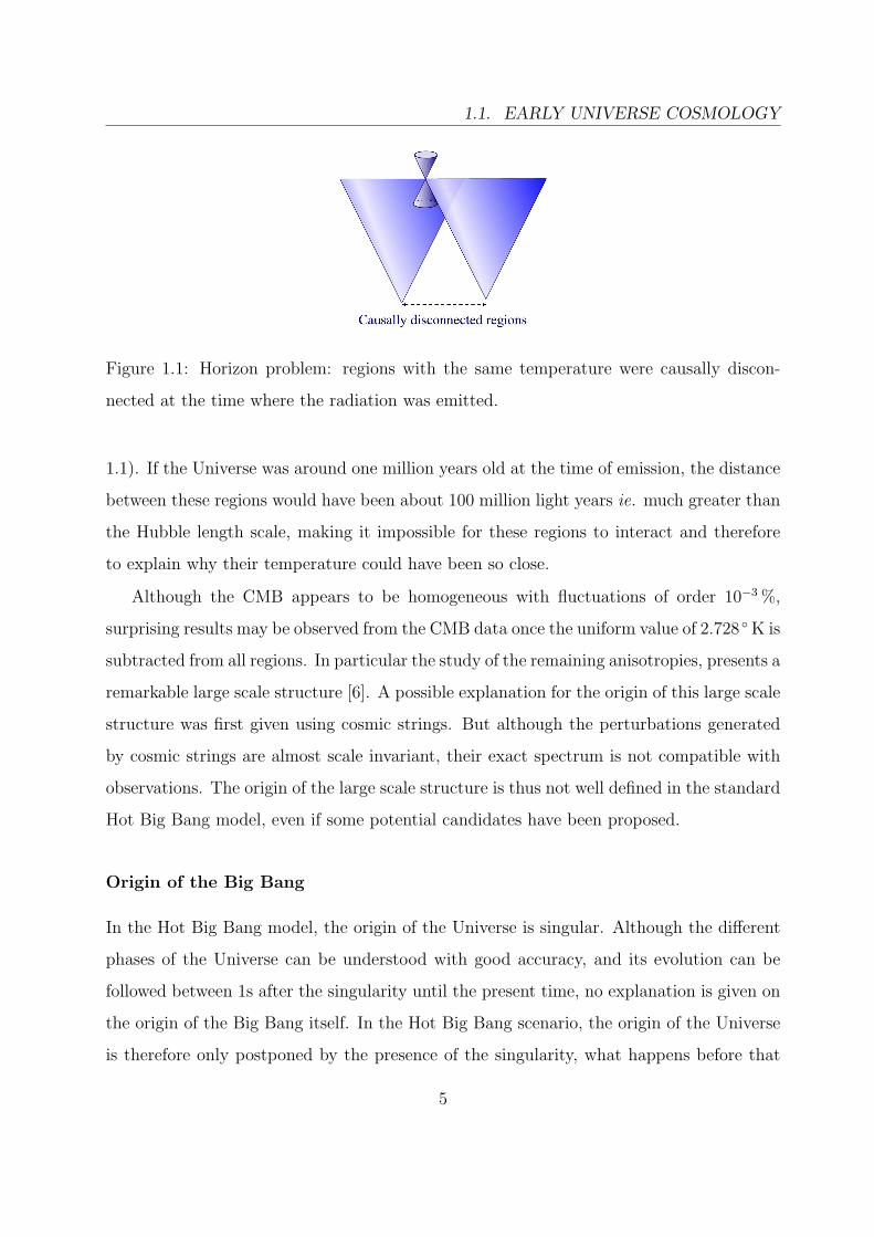
Figure 1.1: Horizon problem: regions with the same temperature were causally discon-
nected at the time where the radiation was emitted.
1.1). If the Universe was around one million years old at the time of emission, the distance
between these regions would have been about 100 million light years ie. much greater than
the Hubble length scale, making it impossible for these regions to interact and therefore
to explain why their temperature could have been so close.
Although the CMB appears to be homogeneous with fluctuations of order 10−3 %,
surprising results may be observed from the CMB data once the uniform value of 2.728 K is
subtracted from all regions. In particular the study of the remaining anisotropies, presents a
remarkable large scale structure [6]. A possible explanation for the origin of this large scale
structure was first given using cosmic strings. But although the perturbations generated
by cosmic strings are almost scale invariant, their exact spectrum is not compatible with
observations. The origin of the large scale structure is thus not well defined in the standard
Hot Big Bang model, even if some potential candidates have been proposed.
Origin of the Big Bang
In the Hot Big Bang model, the origin of the Universe is singular. Although the different
phases of the Universe can be understood with good accuracy, and its evolution can be
followed between 1s after the singularity until the present time, no explanation is given on
the origin of the Big Bang itself. In the Hot Big Bang scenario, the origin of the Universe
is therefore only postponed by the presence of the singularity, what happens before that
5

CHAPTER 1. INTRODUCTION
and what generates it remains mysterious. It is actually extremely difficult to make much
progress on that subject, although this is one of the most intriguing questions. So far
very few acceptable ideas have yet been proposed. As an example, we may suggest the
idea that our Universe might have been created by quantum tunnelling from nothing [7].
This proposal relies on the existence of a Hawking-Moss instanton from which the Universe
could have been self-created.
Dimensionality of our Universe
So far, no remarks have been made concerning the dimensionality of our Universe. From
the every day life point of view, no objections can be made to the fact that we appear to
live in a (3 + 1)-dimensional spacetime, and to date no deviation from four-dimensional
physics have yet been observed, not even at very small physical scales. Since the concept
of extra-dimensions is very hard to picture, the fact that only three spatial dimensions
are observed did not seem to present any problem before models requiring more spatial
dimensions have been suggested. The Hot Big Bang scenario does not give any explanation
for this fact and, as we shall see, very few explanations have actually been proposed. An
anthropic argument might answer half the question: If our spacetime had less than three
spatial dimensions, it is reasonable to assume that life would probably not have developed
and the question of the origin and dimensionality of that Universe would not be posed. For
superstring theory to be a consistent theory, extra-dimensions have to be considered, as we
shall see. The reason why only three of these dimensions are observed remains uncertain
but a more detailed discussion on this subject and on some proposed mechanisms is given
in section 1.3.2.
As we shall see in what follows, an explanation for some of these puzzles is given in the
model of inflation which will be described now. This is no proof of the validity of inflation
nor of the uniqueness of such a model but it is however reassuring to find a model capable
of explaining some of the main features of cosmology, although many questions remain
open and some new puzzles arise.
6

1.1. EARLY UNIVERSE COSMOLOGY
1.1.3 Inflation
de Sitter Cosmology
The idea behind inflation relies on the possibility that our Universe underwent a nearly
de Sitter phase prior to the usual Hot Big Bang evolution. Inflation is not a substitute
of the Hot Big Bang scenario but rather a mechanism that sets the initial conditions
for the usual evolution. Such a phase would be generated if the right hand side of the
Friedmann equation (1.1) was a constant, the scale factor would then grow exponentially,
leading to a de Sitter cosmology [8]. This is for instance the case if the only energy density
present (or the dominant one), arises from a uniform vacuum energy Λ. The scale factor
would then grow in proper time as a(t) ∼ eHt where the Hubble parameter H is constant:
H =√
κ4Λ/3, leading to a uniform expansion of the Universe. Such an evolution has the
advantage of diluting any deviations from flatness as well as any topological defects, giving
an explanation for two of the previous puzzles, although inflation was first proposed only
to solve the monopole problem. Its capacity to solve some of the other puzzles has made
this model specially interesting.
If we suppose that some curvature k was present at the beginning of the Universe, this
would give rise to the following Friedmann equation:
H2 =κ4
3Λ− k
a2. (1.2)
The effective energy density associated with this curvature, ρk = −3k/κ4 a2, would be
exponentially suppressed in comparison with the energy density for the vacuum: ρk/ρΛ ∼
a−2 ∼ e−2Ht. Any deviations in flatness are therefore exponentially suppressed by the
exponential expansion of the scale factor, explaining why the present Universe is observed
to be so flat. Similarly, in such a scenario, topological defects such as magnetic monopoles
could still be produced, but their energy density would be exponentially suppressed in a
de Sitter spacetime, explaining why so few (or none) have yet been observed.
Although the scale factor may be very small in a de Sitter spacetime, the time T needed
7

CHAPTER 1. INTRODUCTION
for it to go to zero back in time is infinite:
T =
∫ a0
0
da
a= H−1
∫ a0
0
da
a=∞, (1.3)
in a purely de Sitter spacetime, it would thus take an infinite proper time to go back to the
singular pointlike Big Bang origin. Since the geometry is actually only approximatively
de Sitter, the actual time to go back to the Big Bang is very large, but finite. This would
still be enough to solve the horizon problem, if at some point before the usual Hot Big
Bang evolution, the Hubble scale had been greater than the physical scale. This would be
possible if ∂t (aH)−1 < 0, ie. if the comoving Hubble length was decreasing in time. This
is in general one of the conditions required for inflation. The Hubble scale can hence be
greater than the physical scale at the beginning of inflation, and so interactions within a
region of the size of the physical scale would be possible. This would hence explain the
large scale homogeneity of the CMB.
A possible explanation for the flatness, the horizon and the monopole puzzles would
therefore be available if our Universe underwent an inflationary period of about 60 efolds
after the Big Bang [8]. Since this is one of the most commonly accepted explanations, we
shall describe below how such a phase could arise.
Inflaton Scalar Field
In order to obtain a nearly de Sitter phase, one needs a vacuum energy density which
dominates the content of the Universe. For a conserved fluid to have such properties, its
pressure p = ωρ should be related to its energy density ρ in such a way that ρ does not
vary. From the conservation of energy, ρ = −3H (ρ + p), this fluid needs to have a pressure
p ' −ρ, in other words, the parameter w for the equation of state should be very close
to w ' −1. This is possible if a scalar field ϕ is present in the theory and dominates the
contributions to ρ and p. The stress-energy tensor will then derive from the action:
Sϕ =
∫dx4√−q
(1
2(∂ϕ)2 + V (ϕ)
), (1.4)
8

1.1. EARLY UNIVERSE COSMOLOGY
where the potential V (ϕ) describes the scalar field interactions [9, 10]. Assuming cosmo-
logical symmetry, the energy density for this scalar field is ρ = 12ϕ2 + V (ϕ) whereas its
pressure is p = 12ϕ2−V (ϕ). In the regime where the scalar field is evolving very slowly, its
kinetic energy may be neglected in comparison with the potential energy, ϕ2 V (ϕ), and
the required property p ' −ρ is thus satisfied. This leads to an almost constant Hubble
parameter H2 ' κ4
3V (ϕ0), as long as the field is moving slowly ϕ ' ϕ0. This scalar field is
often called the inflaton.
In this model, the contribution of the potential should be very important, so the scalar
field can not be stationary at a minimum located at V = 0, (which would be for instance
the minimum for a free massive scalar field with potential V = 12m2ϕ2). Instead one can
imagine a scenario for which the scalar field is located at a non-vanishing minimum of the
potential. Including temperature corrections, the effective potential may spontaneously
change configuration and new vacua can appear. The scalar field can hence tunnel to
a new vacuum after having stayed (for about 60 efolds) in the false vacuum with non-
vanishing vacuum value. In that model, the assumption that the scalar field moves slowly
(or not at all) would hence be valid but we shall see later that this idea does not work. In
many scenarios, the scalar field is instead assumed to star “up the hill” of a slowly-varying
potential and rolls slowly towards the minimum, although few explanations on why the
scalar field would start up the hill are given. The potential should then be very flat and
satisfy some slow-roll constraints [11].
Predictions of Inflation
Although inflation seems to solve three of the previous puzzles, some questions remain
open. The origin of the Big Bang, for instance, is still unaddressed. Inflation has however
the remarkable property to solve a supplementary question which is the origin of the large
scale structure and to model with a surprising accuracy some of the large scale structure
details.
In the inflationary scenario, the large scale structure finds its origin in the curvature
9

CHAPTER 1. INTRODUCTION
perturbations (sourced by the scalar field perturbations). The inflaton is indeed expected
to have very small thermal fluctuations which should be almost the same at every scale
and have a gaussian distribution. The subsequent fluctuations in the curvature could then
explain the anisotropies observed in the CMB measurements [12,13]. The power spectrum
of such perturbations generated within an accelerating de Sitter background is surprisingly
close to current measurements [14,15]. Although one might argue that other theories might
give the same prediction [16, 17], this represents a very important prediction of inflation
and is the reason why it has been the subject of so much interest despite the presence of
some problems (which we shall summarise in the following).
So far no uncontested alternative theories have been proposed and although the origi-
nal inflation scenario has found some failures, some more complicated versions have been
proposed. Among these models, we may in particular point out hybrid inflation, which is
generated by two scalar fields, one responsible for the large vacuum value and the other
one for the thermal perturbations [18]. After tuning, these more elaborated versions of
inflation could model a wide range of different large scale structure observations.
Problems of Inflation
• Interpretation of the inflaton scalar field
One of the most fundamental problems of inflation is the origin of the inflaton scalar
field as no such fundamental spin-0 particle has yet been observed. In the original
scenario [19], A. Guth suggested that the inflaton scalar field could be identify as
one of the fields present on the SU(5) GUT as the Higgs field [20]. In this idea,
the non-vanishing vacuum value for the inflaton would be obtained through the false
vacuum mechanism we explained earlier on. However in that model, the amplitude
of the false vacuum should be tuned to a value much beyond what would be natural
from the GUT scales. Furthermore the decay rate of the false vacuum would be
very important. The interpretation of the inflaton as a possible Higgs candidate has
therefore been dropped. Some other attempts have been given but so far the question
10

1.1. EARLY UNIVERSE COSMOLOGY
remains opens.
• Fine-Tuning
Another fundamental problem of inflation is its requirement of impressive fine-tuning
in its different parameters and initial conditions. The potential needs indeed to sat-
isfy some slow-roll conditions and, at the same time, should be capable of generating
60 efolds of inflation. The original value of the potential should thus be enormous
and especially compared to the present cosmological constant. It seems highly im-
probable that such fine-tuned quantities just happened to take place and to provide
the Universe with such convenient features. The physical intuition seems to suggest
that some fundamental underlying physics is not understood and should explain why
such value could have been picked or provide an alternative mechanism.
• Inflation in question
The previous two problems have put inflation into question despite its accurate pre-
dictions of the large scale structure. In particular the way the initial conditions
should be imposed is subject to important polemics especially since the origin of
inflation itself is not fully understood.
We have mentioned so far only the two main problems of inflation but some other
criticisms exist. In particular, inflation does dilute the topological defects but once
inflation has ended, monopoles could still come back in large numbers. Another
open question is how does inflation end? In the original idea of A. Guth, a natural
ending would occur when the scalar field spontaneously decays into the true vacuum,
however this idea is no longer considered. Instead the scalar field is often assumed
to roll gently down the potential hill and it is difficult to find a natural ending to
inflation. In models of hybrid inflation, such an end is more easy to track since one
scalar field is directly responsible for the shape of the potential.
Despite the success of inflation to explain some of the most important puzzles of cosmology,
some questions remain open. Since the idea of inflation was first suggested, 24 years ago,
11

CHAPTER 1. INTRODUCTION
enormous efforts have been placed into this area to extend this model, fill the open questions
and test its predictions by important observation programs. Despite all these efforts no
real alternative or explanation can yet be given although many new important ideas are
in the process of being tested. String theory, born more than 30 years ago and followed
by Superstring theory 25 years ago has gained an incredible interest as a fundamental
unified theory. The idea that gravity could be associated with other forces (for instance
electromagnetism) in a unified theory is however not new and dates from Kaluza Klein
compactification. As we shall see, these unified models require extra-dimensions [21] whose
implications for cosmology shall be the main focus of this thesis (for a review on extra-
dimensions, see [22]).
1.2 Extra-dimensions and Braneworld
1.2.1 Kaluza Klein Compactification and Extra Dimensions
The notion that our Universe could be embedded in compactified extra-dimensions is not
new. In 1919, T. Kaluza suggested that our Universe could have actually been five-
dimensional with the fourth spatial dimension curled into a circle of radius R H−1
where H−1 is the horizon scale [23]. If R was much larger than our horizon scale, our
Universe would effectively be five-dimensional. When R ∼ H−1, we would not see the
fifth dimension exactly as one of our three spatial dimensions, but some effects would be
present. In particular, to go from one point to another, light could circle on a geodesic
around the compactified dimension any number of times. It would therefore seem to us,
that any object would be repeated with a certain periodicity depending on R. In the case
where the radius of the extra-dimension is of order the Planck scale, we expect to recover
an effectively four-dimensional spacetime as we observe. In that case, the energy required
to excite modes in the extra-dimension is huge and, at low energies, no such “Kaluza Klein”
modes are excited.
12

1.2. EXTRA-DIMENSIONS AND BRANEWORLD
Figure 1.2: Kaluza Klein compactification.
In Kaluza theory, the five-dimensional spacetime would have the metric:
ds2 = Φ dy2 + 2Aµ dy dxµ + gµνdxµdxν , (1.5)
where y designates the extra-dimension and xµ our four-dimensional spacetime. Only
gravity can propagate in the fifth dimension but on our four-dimensional spacetime, elec-
tromagnetism is recovered as a consequence of the presence of the vector field Aµ. Aµ
could indeed play the role of the photon, Φ is what is called the dilaton scalar field, and
gµν plays the role of the graviton. From five-dimensional general relativity, we recover Ein-
stein gravity and Maxwell electromagnetism. An extension of this model was performed in
1926 by O. Klein [24]. In that theory, a pointlike particle in four dimensions is described
as a circle wrapping the fifth dimension. Excitations along this circle (or string) can be
responsible for different characteristics of the pointlike particle. This idea is at the basis
of string theory. In string theory, the higher-dimensionality of spacetime is not a possibil-
ity but a requirement. We shall see for instance in superstring theory, that our Universe
should be ten-dimensional. Since only three spatial dimensions are effectively observed,
one might think that the extra-dimensions should be compactified. However there exists
an alternative: The notion of branes, that we shall describe later. The notion of a domain
13

CHAPTER 1. INTRODUCTION
wall in an extra-dimension can be understood independently to string theory, however the
existence of branes has been motivated by string theory where they represent a hypersur-
face on which open strings end. We shall therefore very briefly review the basic notions of
string theory in the next subsection and see how the notion of branes has emerged.
1.2.2 Basic notions of String Theory
Conformal Invariance and Critical Dimension
At the basis of string theory, is the notion we have already mentioned that particles might
not be pointlike but might be extended objects with their own dimension [25–28]. A
particle line element is given by√−GabXaXb (where a dot is a derivative with respect
to its proper time), Xa being the coordinate of the particle in the (d + 1)-dimensional
target space and Gab its metric. By analogy, the worldvolume of an extended object is
instead the square root of the determinant of the tensor Vαβ = −Gab ∂σαXa ∂σβXb where
σ0 = τ is the proper time of the object and the other σI represent its proper spatial
dimensions. In particular, a string has only one spatial dimension σ1 and the tensor Vαβ is
two-dimensional. A priori, there is no reason to consider a string rather than a membrane
(with two spatial proper dimensions) or any other extended objects, but we shall see that
strings have the very remarkable property to preserve conformal invariance, which is not
the case for any other extended object. Furthermore, despite attempts which have lead to
Matrix theory [29], it has not yet been possible to give a consistent quantised theory for
extended objects with dimensionality higher than two. Finally, string theory is the only
theory able to unify gravity with the other forces of nature. This is the reason why strings
play a very special role in modern physics.
The starting point for the study of string theory is the Nambu-Goto action [30] which,
by analogy to a pointlike particle’s action, is given by
S = −T
∫d2σ
[det(−Gab ∂σαXa ∂σβXb
)1/2], (1.6)
where T = 2πα′ is the string tension and α′, which has the dimensionality of a length
14

1.2. EXTRA-DIMENSIONS AND BRANEWORLD
square, is the fundamental parameter of the theory. Although this action is more intuitive
to derive by analogy to the point-particle action, the presence of the square root makes it
hard to quantise. Instead we may derive the same equations of motion from the Polyakov
action [26]:
S = −T
2
∫d2σ√−hGab hαβ ∂σαXa ∂σβXb, (1.7)
where the worldsheet metric hαβ appears as a Lagrange multiplier in this new action
imposing the constraint X,α ·X,β− 12hγδ X,γ ·X,δ hαβ = 0, (where contractions are performed
with respect to Gab). This implies the conformal relation between the worldsheet metric
and the induced metric: hαβ = Ω2 X,α · X,β, with an arbitrary conformal factor Ω. This
new Polyakov action is clearly invariant under the conformal transformation hαβ → Ω2hαβ,
which would not be the case if the worldsheet was not two-dimensional. This theory
is therefore conformally invariant and is a special case of a conformally invariant sigma
model [31]. When quantising this theory, it seems therefore natural to require that this
symmetry remains preserved. Although this is trivial at the classical level, at the quantum
level, some quantum anomalies break that symmetry [25,26,31]. (Quantum anomalies are
generic to quantum field theories. They arise from regularisation which have to be made
at the quantum level in order to calculate correlation functions, since operators can not be
evaluated at the same point.) For bosonic string theory, it is however possible to cancel
the quantum anomalies and to preserve the conformal symmetry if the dimension of the
target spacetime is fixed to 26 [32,33]. This number seems to come out of nowhere, and in
its derivation, it appears to be an integer only by chance, however this is a very important
result and we shall assume in what follows, that we live in a target spacetime with the
critical number of dimensions for the theory to be conformally invariant at the quantum
level.
Boundary Conditions
In the actions (1.6) or (1.7), some boundary conditions need to be specified for the string
coordinates Xa. In particular we might either think of periodic conditions or Neumann
15

CHAPTER 1. INTRODUCTION
boundary conditions which are both consistent with the variation principle. When the
strings are quantised, the different excitation levels lead to different particles.
• For Neumann boundary conditions, the string is open, and the condition ∂σXa = 0
is imposed at its end points. In that case, the mass square of the string is given
by M2 = (−1 + n) /α′ where n is the excitation number of the string. In particular,
when the open string is in its vacuum state (no excitation), its mass square is actually
negative, leading to the presence of a tachyon. It is the presence of this tachyon which
makes bosonic string theory ill-defined. For n = 1, the string is massless. This degree
of excitation may be parametrised by a vector Aa which defines along which direction
in the target space the string is excited. From the target space point of view, this
corresponds therefore to a massless vector field, in other words this string could be
interpreted as a photon.
• For Periodic boundary conditions, the string is closed and Xa(σ, τ) = Xa(σ + 2π, τ),
if we assume its total length to be 2π. For such a string, excitations can propagate
in two possible directions (clockwise or anticlockwise, which are called left or right
movers), without interfering with each other. The number of right and left excitations
need however to be the same, even if the directions of excitation on the target space
are not necessarily the same. The mass square of the string is then given by M2 =(−1 + 1
2(nL + nR)
)/α′ where nL,R are the excitation numbers on both directions,
nL = nR. The first excited state of a closed string is therefore massless and is
parametrised by a tensor field (with one index for each right and left moving mode).
This tensor field may be decomposed as a traceless and symmetric tensor Sab, an
antisymmetric one Bab and a scalar field S ′. Sab represents a spin-2 massless particle
and is hence a good candidate for the graviton. String theory (or superstring theory)
is the only theory which incorporates gravity. The antisymmetric tensor field Bab
represents what is called the Kalb-Ramond field and S ′ the dilaton scalar field, both
these fields are massless.
16

1.2. EXTRA-DIMENSIONS AND BRANEWORLD
Although this is only the basic description of bosonic string theory, (which presents various
problems), the same general ideas remain valid when its extension to superstring theory is
considered. In particular, the presence of the graviton is a key element of string theory. The
notion of a curved spacetime can for instance be interpreted as a flat Minkowski spacetime
on which closed graviton strings are propagating.
Superstring Theories
Despite being the first theory capable of incorporating gravity in a natural way [34], being
unstable (due to the presence of the tachyon scalar field), and lacking of any formalism to
describe fermions, the bosonic string is not of great interest. Its extension to superstring
models [35] and to heterotic strings, on the other hand, has gained a very popular interest.
Today five different superstring theories have been found: the Type I, with N = 1 super-
symmetry followed by the Type IIA and IIB theories with N = 2 supersymmetry and the
two Heterotic SO(32) and E8 × E8 string theories. For these theories, the critical target
space dimension is 10 rather than 26 [36]. In 1984, M. Green and J. Schwarz indeed showed
that in ten dimensions, not only the anomalies related with the conformal symmetry of the
worldsheet cancel, but as well the target space is free of chiral or gravitational anomalies
for some special groups [37].
The main difference between these theories relies on which boundary conditions are
imposed (fermions have more complicated boundary conditions), and whether the strings
are oriented or not. In heterotic strings, which are theories for closed strings excursively, the
left and right movers do not belong to the same theory, one satisfies superstring conditions,
while the other belongs to the bosonic sector. The heterotic theories however remain ten-
dimensional. Among these theories the only one that contains open strings is the Type
I, all the others are exclusive to closed strings. The open string need however to contain
closed strings as well since an open string may close itself up and form a closed string. Due
to the fermionic nature of superstrings, open strings have charges (or Chan-Paton factors)
attached at their end points.
17

CHAPTER 1. INTRODUCTION
T-duality
The last crucial point we shall briefly mention about string theory is the notion of T-
duality [38]. We have seen that particles may be interpreted as strings with different
vibration or excitation numbers. Furthermore for the theory to make sense, the dimension
of the target spacetime should be 10 (or 26)-dimensional. Since we only observe three
spatial dimensions, it makes sense to consider that some of these dimensions might be
compactified on a circle of radius R, just as the Kaluza Klein compactification. Strings
might therefore wind around these compactified dimensions. The energy needed for a
particle to wind around a compactified dimension is proportional to R. Inversely, for
a particle to be excited along the compactified dimension, the energy required goes as
α′/R. If we consider a string with m winding modes, and n excitation number along that
compactified direction, its energy will therefore be the same as the one of a string with n
winding modes around a compactified direction of radius α′/R and excitation number m.
Torii of radius R will therefore share the same energy spectrum as torii of radius α′/R, with
the only difference that the role of winding modes and vibrations modes will be inverted.
The duality R → α′/R plays a crucial role in string theory and in particular the fixed
point of the symmetry, at R =√
α′, suggests the existence of a smallest length scale for
theories of closed strings on a torus (since any length scale smaller than√
α′ is equivalent
to a length scale bigger than√
α′), although some branes could probe smaller scales in
other situations.
This T-duality actually relates the different closed superstring theories:
T-dualitytype IIA ←→ type IIB
heterotic SO(32) ←→ heterotic E8× E8.
1.2.3 M-theory and Orbifold Branes
As already mentioned, five well-defined different string theories exist. We might therefore
ask the question whether these theories are really independent or if they are not part
18

1.2. EXTRA-DIMENSIONS AND BRANEWORLD
of the same fundamental theory and represent different limit of it. This is a sensible
question since T-duality relates some of them. Furthermore only a perturbative approach
to string theory is known. The underlying fundamental theory could then be the answer of
the quest of a non-perturbative approach to string theory incorporating the five different
string theories known so far. This theory has been named “M-theory”, but apart from its
known string theory limits, very little is actually known about it, (for a review, see [39]). It
has been shown that an additional limit of M-theory could be found, and at low-energy, M-
theory should look like 11-dimensional supergravity, (see for instance [40]). The underlying
fundamental theory should therefore be 11-dimensional, and appear ten-dimensional only
in some special limit such as for the five different string theories [41].
Any object in the ten-dimensional string theory description should therefore behave as
an extended object in the 11-dimensional M-theory. Thus, a string in the ten-dimensional
string theory should, for instance, look like a (2 + 1)-dimensional membrane in M-theory,
and similarly for any Dp-brane in string theory. In particular, a special interest can be
given to what the heterotic E8 × E8 should look like from the 11-dimensional M-theory
point of view. In 1996, P. Horava and E. Witten suggested that from the extended M-
theory point of view, the heterotic E8 × E8 string theory would appear as a Heterotic
M-theory, compactified on a S1/Z2 orbifold with orbifold-branes located at the fixed point
of the symmetry [42]. The extra-dimensional should be larger than the other compactified
dimensions (compactified on a Calabi-Yau), suggesting that there could be a regime where
the Universe would appear five-dimensional. This model has opened an entire new set of
possibilities for the study of orbifold branes. It is motivated by advances in this subject,
that so much interest has been given to braneworld cosmology. The main part of this thesis
is indeed devoted to the study of orbifold branes in the Randall Sundrum model which is
a very simple five-dimensional version of the real Heterotic M-theory model.
It might seem strange that the same fundamental theory would be capable of describing
all of the five superstring theories, especially when one of them contains open strings while
the others not. The reason for that is the existence of another duality, the weak/strong
coupling duality (or S-duality), that relates the different theories [43]. In particular, the
19
CHAPTER 1. INTRODUCTION
heterotic SO(32) theory is dual to the open (and closed) type I superstring theory. At weak
coupling, open strings in the heterotic sector might exist but they are highly unstable and
hence quickly decay into closed strings. The type I theory might be the strong coupling limit
of some region of M-theory. In order to incorporate open strings in a more fundamental
way to the theory, we shall see that D-branes should be considered.
1.2.4 D-Branes as the End Points for Open Strings
Dirichlet Boundary Conditions
S-duality relates the Type I open string theory to the heterotic SO(32) closed string theory.
The notion of T-duality on open strings is however less clear. For T-duality to work, the
string needs to wind around a compactified direction and not be able to unwind without
interactions. When Neumann boundary conditions are imposed at the end point of strings
(requiring their spatial momentum ∂σXa to vanish at that point), open strings can unwind
without any interaction. However this would not be the case if their end points were
instead fixed. For that, Dirichlet boundary conditions may be imposed, and T-duality
could have for effect to swap Neumann and Dirichlet boundary conditions. If d is the
spatial dimension of the theory (ie. d = 9 for superstrings), we may consider that (p + 1)
of the string coordinates satisfy Neumann boundary conditions (0 ≤ p ≤ d), while the end
points of the remaining (d− p) coordinates are constrained to Dirichlet conditions:
∂σXa (τ, σ)|σ=0,π = 0, a = 0, · · · , p (1.8)
Xb (τ, σ)∣∣σ=0,π
= Xb (τ) , b = p + 1, · · · , d. (1.9)
The end point of the string is therefore fixed on a p-dimensional hypersurface called
D(irichlet)p-brane [28,44]. The study of D-branes will present interesting links with gauge
field theories. In the previous example (1.8 - 1.9), the boundary conditions were taken
to be the same on both ends of the string, but there is actually no reason to impose this
condition and we might as well take into consideration “mixed” coordinates for which a
Neumann condition is imposed at one end and a Dirichlet one at the other end. The special
20

1.2. EXTRA-DIMENSIONS AND BRANEWORLD
case considered until now, for which all coordinates had Neumann boundary conditions,
represents the situation of spacetime entirely filled with a Dd-brane. In that case the
strings are completely free to move in the entire spacetime.
Figure 1.3: Closed strings propagate in the entire spacetime while the end points of open
strings are attached to D-branes.
Maxwell Gauge Theory
After quantising the open strings on Dp-branes, we may consider the first excited state
(analogous to the photon massless state we presented earlier). If the string is excited along
the directions tangent to the Dp-brane, a (p + 1)-dimensional massless vector field Aa will
parametrise the vibrations. This field will have (p − 1) independent variables. From the
Dp-brane perspective, this field will therefore play the role of a Maxwell gauge field. If
on the other hand, the string was excited along the direction normal to the Dp-brane,
the (d − p)-dimensional vector field Ab, parameterising the vibrations, will not carry any
21

CHAPTER 1. INTRODUCTION
indices along the brane. This field having (d− p) independent variables, the Dp-brane will
therefore see (d − p) massless scalar fields. We therefore recover in a completely natural
way a p-dimensional Maxwell gauge theory on the Dp-brane. This is a remarkable result,
explaining the special interest which has been given to these objects.
So far we have only considered one Dp-brane alone. If we extended this model to N
parallel D-branes, we could see that the same result would remain valid, and in particular
if N such D-branes were coincident, they will carry a U(N) gauge field.
D-branes are hence extended objects of superstring theory which carry charges (electric
and magnetic Ramond-Ramond charges) [45] and present very interesting properties. In or-
der to understand their implications to cosmology some special cases should be considered,
and the model will be largely simplified.
1.2.5 Hierarchy Problem and Large Extra-dimensions
Hierarchy Problem
One of the most confusing problem of particle physics is why two fundamental quantities,
sharing the same unit, do not share the same order of magnitude. Naıvely, one would expect
all numbers coming from a fundamental theory to have the same order of magnitude. This
is not the case for the Planck and the electroweak scales. The electroweak symmetry breaks
at an energy scale of order 250 GeV (around which the vacuum expectation value of the
Higgs field is hence taken). The Planck scale (at which quantum gravity effects come in),
on the other hand, is of order 1018 GeV. The Higgs mass is hence about 1016 times lighter
than the Planck mass.
Compactified Extra-dimensions
So far, even though we considered the spacetime to have extra dimensions, we implicitly
assumed the extra dimensions to be compactified on torus of small radius a la Kaluza
Klein (or compactified on a Calabi-Yau manifold). These compactifications were made
so that effectively our Universe would remain four-dimensional, the radius of the extra-
22

1.2. EXTRA-DIMENSIONS AND BRANEWORLD
dimension being too small for Kaluza Klein modes to be excited at low energies. In these
models, the four-dimensional physics is unaffected by the presence of extra-dimensions, and
in particular problems occurring in usual physics (such as the hierarchy problem) remain
unsolved. Although it is convenient to recover usual four-dimensional theory in some limit,
the presence of these extra-dimensions may appear as “wasted”.
Large Extra-dimensions
Motivated by heterotic M-theory, (where the 11th-dimension could be compactified on
an S1/Z2-orbifold), there has recently been an increased interest to models where some
extra-dimensions could be “large”. If all forces of nature, but gravity, were confined on
a four-dimensional hypersurface, the usual physics will apply for them. Gravity (being
propagated by closed strings), on the other hand, could be allowed to evolve in the entire
spacetime. This may be justified by the fact that gravity is the weakest force of nature
at short-distances and has been tested only up to distances of order of a millimetre3 [47].
It is hence possible that departures from Newton’s law might occur at lower scales, which
would be the case if gravity was not confined to a four-dimensional spacetime. This new
idea, suggested by N. Arkani-Hamed, S. Dimopoulos and G. Dvali, [48], has motivated the
study of large extra-dimensions, in which gravity might “leak off”. The key point of this
idea is that the presence of wrapped extra-dimensions could resolve the hierarchy problem.
The higher-dimensional Planck scale could indeed be of the same order of magnitude as the
electroweak scale if one extra-dimension was of the size of the solar system while all other
extra-dimensions would be compactified on a small torus. This extra-dimension would be
huge, but if two dimensions were taken to be large, the hierarchy problem could be resolved
if their size was only of order of the millimetre.
It is based on this idea that different models where suggested, such as [49] and especially
such as the first and second Randall Sundrum models [50, 51]. In these models, (which
3The Eot-Wash Short-range experiment has measured the strength of gravity for distances slightly
smaller than 0.2 millimetre and have observed no deviations from the Newton’s law, but recent experiments
are still testing gravity at sub-millimetre scales [46].
23

CHAPTER 1. INTRODUCTION
we shall describe in great detail in chapter 2), all forces of nature (not counting gravity)
are confined on the orbifold branes, where the presence of the orbifold is motivated by
heterotic M-theory. This has the advantage of avoiding charges and form fields which are
usually present when D-branes are considered. Although this model is greatly simplified
compared to any realistic model emerging from string/M-theory, it has the great advantage
to be a consistent toy model on which the idea of large-extra dimensions may be tested
in cosmology. Later extensions of this model have been proposed to solve the hierarchy
problem in more realistic scenarios [52].
A predecessor of the Randall Sundrum scenario was the model suggested by A. Lukas
et.al. [53]. After deriving a five-dimensional effective theory of the 11-dimensional Horava
Witten’s theory, a five-dimensional cosmological solution was studied and shown to repre-
sent a consistent solution for early Universe cosmology. In their model the boundary branes
are actually three-brane domain walls on which gauge and matter fields are confined. The
Randall Sundrum scenario represents a very special case of their general solution, for which
all gauge fields are set to zero.
But the idea that our Universe could be a four-dimensional membrane in a higher-
dimensional world is much older [54]. One of the first toy models which considered this
possibility was given by G. Gibbons and D. Wiltshire in [55]. In that work, the Einstein-
Maxwell equations are solved and give a consistent solution, for which the Kaluza Klein
corrections may be ignored if the membrane has curvature or if a negative cosmological
term is present in the higher-dimensional spacetime. This idea is present in the Randall
Sundrum as well, for which a negative cosmological constant is used in the bulk.
1.3 Brane Gas and Dimensionality Puzzle
In the previous section, we showed how the concept of braneworlds could be derived from
string theory and in particular, we have suggested the idea that our Universe could be a
four-dimensional membrane embedded in a higher-dimensional world. Although this might
explain why we only see three spatial dimensions despite the fact that the true world
24

1.3. BRANE GAS AND DIMENSIONALITY PUZZLE
might be higher-dimensional, this does not explain why a four-dimensional membrane
was considered in the first place. Unless some specific mechanisms are found to explain
why four-dimensional branes are favoured with respect to other dimensional branes, the
puzzle remains open. In this section we shall summarise the different ideas that have
been proposed to explain why only three spatial dimensions are observed. There have
been two main ways of attacking this problem. In the first one, developed well before
M-theory was proposed, R. Brandenberger and C. Vafa suggested a reason why only three
spatial dimensions could grow large [56]. But the way of attacking the problem has taken
another direction since a possible underlying theory with a relatively large extra-dimension,
(which would be unobserved in some limit), has been pointed out. Instead of showing why
a scenario with only three large spatial dimensions is favoured (or is the only possible
scenario), people have tried instead to understand why three-branes (on which we might
live, or on which usual physics laws are derived) might be favoured compared to higher-
dimensional branes. All these ideas rely strongly on the notion of brane gas (as an extension
of the string gas concept) which we shall describe first.
1.3.1 Brane gas
Conservative and democratic initial conditions
In the context of string cosmology, the first question one might ask is which initial condi-
tions should we consider. In the standard Hot Big Bang scenario, the Universe is initially
extremely hot and dense and hence a homogeneous and isotropic hot gas of matter is usu-
ally taken for initial conditions. The same idea may apply here and one might assume
the spacetime to be filled with a homogeneous gas of strings. This initial condition is
hence “conservative” as argued by the authors of [56, 57]. But since the realisation that
D-branes must play an active role in string theory, the notion of a gas of strings has been
extended to a gas of branes, (where strings are similar to D1-branes, putting aside the is-
sue concerning the brane charge). In this assumption, branes of different dimensionalities
are generally considered to be initially present with a comparable density so no brane is
25

CHAPTER 1. INTRODUCTION
favoured initially.
We would like to understand why only three spatial dimensions are observed, or in other
words why three spatial dimensions seem to be special and distinguish themselves from
the nine spatial dimensions necessary for string theory. For that, one should start with a
“democratic” treatment of all the spatial dimensions, (“democratic” as argued again by
the authors of [56, 57]). Being compactified or not, all dimensions should be considered
exactly the same way in the initial conditions. Hence either all nine dimensions should be
uncompactified or all of them should be compactified the same way. In particular, if all
dimensions are compactified, a natural assumption would be to take them compactified on
a torus of radius R ∼√
α′. This is a reasonable assumption since the only fundamental
scale of string theory is the length scale√
α′, we might therefore expect all dimensions to
be compactified on a torus of this size. This respects the “democratic” condition.
From this initial condition, several proposals have been given to understand how three
spatial dimensions might separate themselves out. But first we might raise the question of
how this brane gas was created in the first place. In the next subsection will shall therefore
follow the argument by [58] where from a configuration including only spacetime filling
branes, the creation of a brane gas might be understood. In particular, we shall see how
branes of different dimensions might be favoured and hence their density might not be the
same.
Creation of D-branes
In order to understand how brane-antibrane pairs might be produced, we shall follow the
study of [58]. Working in the framework of superstring theory, with nine uncompactified
spatial dimensions, they assume, as a starting point, that all open strings satisfy Neumann
boundary conditions. Or in other word, that the space is initially filled by D9-branes and
D9-branes (antibranes). The initial state presents actually N coincident D9 - D9 pairs.
This configuration is stable at high-temperature but as the temperature cools down,
pairs of D-branes and anti D-branes of lower dimensions are produced. Similarly to a
26

1.3. BRANE GAS AND DIMENSIONALITY PUZZLE
particle-antiparticle pair, a brane-antibrane pair is indeed an unstable configuration at low-
energy, and the initial state possess tachyons which are related to this instability. At high
temperatures, the tachyon is at the minimum of its potential and the configuration is stable,
but when the temperature cools down, the potential is deformed and the tachyon is no
longer at the minimum but at the maximum. The tachyons hence decay to the true vacuum
leading to the annihilation of the D9-D9-brane pairs. But depending on the symmetry
group of the vacuum, different regions of the spacetime may take different topological
configurations and hence topological defects can be created. Since N coinciding D-branes
have an U(N) group, the initial vacuum symmetry group is U(N). We denote by πk(M)
the different ways Sk may be mapped on the group M, (πk(M) is the homotopy group
of M). The different ways S1 may be mapped onto U(1), for instance, is characterised
by the winding number (which is a topological invariant) thus π1(U(1)) = Z. As long
as πk(M) is non-trivial (ie. there exists different possible maps), the tachyon will take
different topological values on different regions of space hence creating a topological defect
of codimension (k + 1), or a D(d − k − 1)-brane, at the intersection of these regions (for
a review on topological defects see for instance [59]). In particular, a D3-brane will be
created if π7 (U(N)) 6= 0, which is indeed the case if N ≥ 3, (π7 (U(N)) = Z). With this
mechanism, only D-branes with odd spatial dimensions will be created. This mechanism
explains how D7, D5, D3 and D1-branes can generically be created out of the initial stable
state. But the way they exactly form and the probability for such a creation depends
on how many regions need to intersect. Branes of lower dimensions require more regions
to have a common intersection (a codimension k object can be seen as the intersection
of (k + 1) regions, so the creation of a D3-brane requires seven regions with different
topological configurations to intersect, while the creation of a D7-brane requires only three
such regions). The creation of D7-branes would hence initially be favoured unless some
energetic and entropic arguments are taken into consideration. This will be performed in
what follows in order to understand why lower-dimensional branes might be favoured.
However the same mechanism described for the decay of D9-D9 pairs, can now apply
for the daughters brane pairs. In particular pairs of D7-D7 branes may decay and give
27

CHAPTER 1. INTRODUCTION
rise to new topological defects or D-branes of lower dimensions. This will hence create a
cascade of daughter branes of lower dimensions.
In this mechanism, the creation of D-branes does not lead, in general, to a homogeneous
gas of branes of different dimensions. The initial conditions considered for this scenario
may as well appear not very natural. It gives however a consistent mechanism for the
production of a brane gas which could be considered in order to understand why only
three spatial dimensions are observed.
1.3.2 String theory contributions to the dimensionality puzzle
Annihilation of extended objects
We shall now focus on the “dimensionality puzzle”, trying to understand either how three
dimensions may distinguish themselves or whether D3-branes are favoured in some scenar-
ios.
Both these ways of attacking the problem rely on the similar idea that strings or other
extended objects may not annihilate for large dimensions but can for lower dimensions.
In order to understand this, we may use the analogy with monopoles, comic strings and
domain walls in standard four-dimensional cosmology. As already mentioned, in three
infinite spatial dimensions, the probability for two monopoles to “collide” is very weak and
in general we consider that monopoles do not decay, thus the magnetic monopole puzzle.
Two cosmic strings, on the other side, (unless they are parallel to each other) will interact
and can annihilate. The same will hold for any extended object of dimension p such that
2(p + 1) ≥ (d + 1), where d is the spacetime spatial dimension. When there is equality,
2(p + 1) = (d + 1), such as for strings in d = 3 dimensions, the collision will happen only
at an instant, but for 2(p + 1) > (d + 1), the intersection happens at all time, this is for
instance the case for domain walls (with p = 2), their intersection can be seen as a 1-brane
(or string). The same will be true in higher dimensions, we thus expect extended objects
with p spatial dimensions (or p-branes) with 2p < (d−1) to survive in a (d+1)-dimensional
spacetime. For larger objects, on the other hand, they will interact and annihilate.
28

1.3. BRANE GAS AND DIMENSIONALITY PUZZLE
Brandenberger Vafa mechanism
Long before the idea of branes had gained much interest, R. Brandenberger and C. Vafa
suggested a proposal [56] to understand why only three large spatial dimensions can be
large. Their starting point was the assumption that at the beginning all nine spatial
dimensions were small and probably compactified on a very small torus of radius R ∼√
α′. Strings will then naturally wind around this torus, preventing the dimensions to
expand since the energy required for a winding mode would grow as R/α′. Spontaneously,
however some dimensions can tunnel to a state where they grow a bit larger. When this
happens, strings wrapping these dimensions compress them back to their normal size; or
this is what happens in the usual case. But if three or less spatial dimensions grow large,
strings wrapping these dimensions may annihilate and let these dimensions “free”, as can
been seen in fig. 1.4. Indeed, if we consider strings (extended objects with p = 1), in
Figure 1.4: Two winding and antiwinding modes can intersect in three or less dimensions
and form a loop (plus radiation).
dimensions lower that d ≤ 2p + 1 = 3 they may interact with each other and hence
annihilate. This is not the case, however, for dimensions greater than three, and is hence an
argument explaining why no more than three spatial dimensions may grow large. Of course,
only two or one dimension might have grown large, but if we imagine a scenario where
29

CHAPTER 1. INTRODUCTION
the small compactified dimensions may spontaneously grow large with a non vanishing
probability, there would be as many dimensions growing large as possible, hence three
dimensions. Another argument relying on the anthropic idea has already been mentioned.
In this mechanism, the other dimensions will remain small and “compressed” by the strings
winding around them. The pressure applied by the strings on the compressed dimensions
might even help the expansion of the other ones.
In this scenario, although some dimensions are capable of expanding and becoming
large, they will still remain compactified. For this to be consistent with present observa-
tions, the radius of their present compactification must be larger than the Hubble radius.
In such a case, we would not be able to notice this compactification and our Universe would
effectively appear to have three infinite dimensions.
The notion of T-duality can be extended to branes [57] and in this mechanism, one
can imagine instead that a brane gas is filling the spacetime and wrapping compactified
dimensions. The argument will then be exactly the same since strings are the extended
objects with the least dimensions, they can still prevent more than three dimensions to
expand while higher-dimensional branes can annihilate.
In the context of heterotic M-theory, the nine-dimensional compactified spacetime de-
scribed above could play the role of the orbifold fixed point of the Z2 symmetry imposed
on the 11th dimension. If only three out of the nine dimensions were allowed to expand, in
heterotic M-theory this would effectively correspond to the presence of a three-dimensional
braneworld (at the orbifold fixed point) embedded in a five-dimensional spacetime.
Early simulation works have confirmed the hypothesis of this model [60]. However more
recent work seem to suggest that this mechanism can indeed happen but its probability
appears to be weak [61].
Majumdar Davis mechanism
Since the appearance of branes as a “popular” object of string theory, another way of
explaining the puzzle has been proposed. Although different alternatives to the problem
30

1.3. BRANE GAS AND DIMENSIONALITY PUZZLE
have been suggested the main idea behind them is similar. Working in the framework of
superstring theory (in particular we will choose type IIB), with nine uncompactified spa-
tial dimensions, the different proposals rely on the same idea that at some point the entire
spacetime could have been filled with a gas of branes and antibranes, but the different sce-
narios suggest slightly different initial conditions and evolutions. Nonetheless, they all have
the final conclusion that D3-branes are favoured compared to other (higher-)dimensional
branes, although we should as well point out that D7-branes play an important role.
We have seen earlier how the study of [58] could explain the creation of a brane gas
from the decay of pairs of D9-D9-branes. In that mechanism, branes of lower-dimensions
were however not necessarily favoured in comparison to the higher dimension ones. In
order to explain how D3-branes might be favoured, one needs to rely on energetic and
entropic arguments as is done in [58]. To perform this last step, they compute the entropy
of a gas of Dp-branes and show that it goes as p−1. They can then conclude that the
probability of ending in such a configuration is exponentially suppressed compared to the
probability of ending in the same configuration with instead a gas of Dq-branes with q < p.
Lower-dimensional branes are hence favoured as long as the initial state possess a large
number N of D9-D9 pairs.
In later work [62], they consider the annihilation of brane-antibrane pairs. Although
the creation of higher-dimensional branes is favoured in comparison to lower ones, their
calculation showed that D-branes of higher dimensions annihilate more rapidly than lower-
dimensional ones. Starting with a gas of branes of different dimensionality, at late times,
the spacetime might be filled with only lower-dimensional ones. It is relying on this last
idea that the proposals in the next subsection have been suggested.
Annihilation of brane-antibrane pairs
The previous argument, relying on the annihilation of D-D-brane pairs, is at the origin
of new proposals [63, 64]. In that case, a gas of D-branes and antibranes of arbitrary
dimensions is directly considered as the initial condition mentioned earlier.
31

CHAPTER 1. INTRODUCTION
Spontaneously, pairs of branes and antibranes can then annihilate and using a simple
dimensional argument, only branes of dimension three or lower are expected to survive.
This is a simple consequence of the fact that in a (d+1) = 10-dimensional spacetime, only
extended objects of dimension p ≤ (d− 1)/2 can miss each other and hence survive. The
other Dp-branes will indeed either intersect at all times or interact at one point but will
eventually disappear, creating at the same time the entropy of our Universe.
This is the proposition given by [63] and then extended by [64] to expanding spacetimes.
In this last paper, an argument relying on the energy density of the different Dp-branes is
used in order to select the most probable configuration in an expanding ten-dimensional
spacetime. In their proposal, the Dp-brane with the highest energy-density is assumed to
be the most favourable one. They then compute the energy density of the different Dp-
branes in an expanding Universe and point out that the total energy density is dominated
by the D3-branes and D7-branes, which are hence the most favourable branes.
The argument goes as follows: If the spacetime is filled with a (homogeneous) fluid with
equation of state p = ωρ where p is its pressure and ρ its energy density, the scale factor
a will scale as a ∼ t2/d(ω+1), where t is the proper time and d the spacetime dimension
(d = 9). For ω < ωc = −1 + 2/d, the expansion accelerates, we will hence consider only
cases for which ω ≥ ωc. A homogeneous distribution of Dp-branes, that do not interact, can
be considered as a fluid with ωp = −p/d and energy density ρp ∼ ap−d. If the Dp-branes
interact, ie. for p > 3, their energy density scales instead with the Hubble parameter
and not the scale factor: ρp ∼ (H−1)p−d ∼ tp−d. If no branes where interacting, the
higher-dimensional branes will hence be favoured in an expanding spacetime since their
worldvolume is considerably larger, but interactions modify this argument. If at some point
spacetime is dominated by D3-branes, effectively the spacetime would be filled with a fluid
with ω = −1/3. The energy density of the D3-branes will hence scale as ρ3 ∼ a−6 ∼ t−2.
Among the interacting branes, the only ones which would have a comparable energy density
are the D7-branes: ρ7 ∼ t−2 and the higher-dimensional ones. However, one expects the
D8-branes not to be present in type IIB string theory (which only contains branes with odd
spatial dimensions). The D9-branes are different since they are space filling and overlap
32

1.4. BRANE INFLATION
entirely, the authors of [64] hence argue that their energy density is zero. The D3-branes
together with the D7-branes are therefore favoured in that situation.
Even if the spacetime is initially not dominated by D3-branes, ω > −1/3, the D3-
branes will still have the greatest energy density (this time even compared to D7-branes),
and the spacetime will eventually be filled with mainly D3-branes. Their initial assumption
is hence reasonable and gives a very simple argument explaining why D3 and D7-branes
are the branes dominating the spacetime energy density.
These arguments only give a rough proposal on how one might attack the problem and
explain why we are living in (3 + 1)-dimensions, but at least they suggest that a possible
solution to the puzzle might be found in the future. Several issues should be studied in
more detail, such as what would happen with the last mechanism if some dimensions were
compactified, and if branes interactions were considered in a more general way. But for
the purpose of this thesis we will concentrate on branes with only three spatial dimensions
and motive this choice by the previous arguments.
1.4 Brane Inflation
Motivated by the arguments of the previous section, we now study the contribution of
three-branes to cosmology. For this, we only give a brief overview of the leading models
which have first been proposed in the context of brane inflation or its alternative. This will
not be an exhaustive presentation as we will only concentrate on specific models, which
have been greatly extended since.
1.4.1 Dilaton and Moduli Fields
One of the most interesting features of string theory is its scalar fields abundance which
arises naturally without the need for any specific assumptions. This seems to be a very
different situation from other areas of physics where scalar fields are assumed to be present,
but their origin can not be explained. The presence of these scalar fields in string theory
33

CHAPTER 1. INTRODUCTION
can for instance be associated with the presence of compactified dimensions. The moduli
fields are indeed related to the size of these dimensions. Unless some non-perturbative
effects are considered, the compactification radius is free to vary. In terms of the moduli
fields, this imply that their potential should be flat. In string theory, the strength of the
gravitational coupling may be freely redefined. Another scalar field, the dilaton, can thus
be associated with this degree of freedom. And one should expect its potential to be as
well flat. The dilaton is indeed a massless scalar field. String theory hence predicts the
existence of massless moduli and dilaton scalar fields. Their existence is at first puzzling
since no massless scalar fields are observed. But if supersymmetry is broken, their potential
is expected to be modified and such fields might becoming massive. Such supersymmetry
breaking could be generated by non-perturbative effects. One of the most important issues
in this subject is the necessity of stabilising these fields. Much effort has indeed been
devoted to the study of realistic models capable of generating an effective potential for the
dilaton, with a minimum where the dilaton may sit. On the other hand, the flatness of
the moduli and dilaton field potentials could have a very interesting application. A flat
potential is indeed one of the most important requirements of inflation. Dilaton and moduli
fields can thus be seen as very good candidates for the inflaton scalar fields [65], this is
very interesting since the origin of the scalar field in inflation remains an open question.
1.4.2 D-brane Inflation
One of the first proposals that has made use of the notion of D-branes to cosmology is
the one suggested by G. Dvali and S. Tye in [66]. Their idea is to derive inflation from a
model including two D-branes. They first consider two coinciding D3-branes embedded in
a bulk with N large extra-dimensions (and suppose that N ≥ 2, hence giving a reasonable
explanation to the hierarchy problem). Calculating the forces between the branes, they
show that this configuration is stable. However, this might not be the initial conditions,
and to start with, they consider the branes to be separated by a distance r while they
still remain parallel. As mentioned previously, one of the most interesting contribution of
34

1.4. BRANE INFLATION
D-branes to cosmology could be the interpretation of this moduli field (the distance r or
the size of the extra-dimension) as playing the role of the inflaton scalar field.
The supersymmetric configuration will be BPS (Bogomolny-Prasad-Sommerfeld [67,
68]), if the contribution from the different forces between the branes cancels out and leads
to a static and stable configuration where the branes are on top of each other. The different
interaction sources between both D-branes are the followings:
• The modes localised on the branes do not couple when the branes are largely sep-
arated. When they get close to each other r → 0, on the other hand, these modes
couple and give a negative contribution to the vacuum energy of the brane which
cancels with the positive branes tensions. When the branes are close, this contribu-
tion vanishes, but when they are separated, this gives a contribution to the potential
V (r) = 2λ where λ is the branes’ tension.
• As already mentioned, D-branes have charges (Ramond-Ramond charges) which will
create a repulsive force between the branes and hence give a negative contribution
to the potential V (r) ∼ −2r2−N .
• Dilaton closed strings can as well be exchanged between both D-branes and contribute
positively to the potential V (r) ∼ r2−N .
• Finally, the exchange of graviton closed strings gives rise to a gravitational attraction
between the branes V (r) ∼ r2−N .
The three last interaction terms therefore cancel in the supersymmetric BPS configura-
tion and since the first term vanishes when the branes are close (or on the top of each
other), this leads to a static configuration at r = 0. But when non-perturbative effects are
generated, supersymmetry could be broken. The bulk modes will get massive and create
instead a Yukawa potential of the form r2−Ne−mr, where m is their effective mass after
supersymmetry breaking. This affects both the dilaton strings and the charge exchange
and the effective potential between the branes for large brane separation hence becomes:
V (r) ∼ 2λ + α rN−2(1 + e−mΦr − 2e−mRR r
), (1.10)
35

CHAPTER 1. INTRODUCTION
where α is a constant and mΦ, mRR are the different fields masses after supersymmetry
breaking. Although the exact details of this calculation are very hard (if not impossible)
to calculate, this suggest a mechanism which could lead to a very flat potential (1.10) in
which the inflaton scalar field (associated to r) could evolve and create a scale invariant
power spectrum. Another beautiful aspect of this model is its graceful exit from inflation,
which would naturally happen when the branes get close to each other. When r → 0, the
contribution of the first term is modified and we should include the contribution of the
localised modes on the branes which vanish exponentially with r. For small r, this will
lead to an exponential contribution to the potential which could hence be steep, inflation
would stop and the reheating period will start.
1.4.3 Brane - Antibrane Inflation
Despite the elegance of the previous scenario, its lack of proper non-perturbative calcula-
tion irrefutably represents a heavy down side. This weakness can be cured if one considers
its natural extension using instead a non coincident brane-antibrane pair [69–71]. Although
the work in [69] takes for initial conditions a set of non-coincident parallel D-branes and
antibranes, the main results remain the same. In [70], it is shown that the different in-
teraction sources from the previous D-brane pair model remain the same although the
interaction between the charges on each branes generates now an attractive force. Hence
the charge contribution does not cancel out the contribution from the dilaton and graviton
exchange in the BPS configuration. In that case, a simple naıve calculation in perturbative
theory can be performed and gives rise to a Newtonian potential (plus a positive constant).
Thanks to the presence of the positive constant, the potential will prevent the branes from
separating too much, and hence avoid a “runaway” form. Unfortunately, the slow-roll
conditions required for inflation to work are not satisfied (although the potential is flat, its
second derivative is not small enough unless the distance r between the branes is taken to
be much larger than the size of the dimensions perpendicular to the brane, which is not
possible). In order to remedy this problem, a more elaborate calculation should be made.
36

1.4. BRANE INFLATION
In particular, if the large extra-dimensions (perpendicular to the branes) are compactified
on a torus, one should include in the calculation the different images of the branes in the
covering space of the torus (especially if the distance between the branes is comparable to
the torus radius). When this is taken into consideration, one gets instead a potential which
is quartic in the brane separation r and hence satisfies the slow-roll conditions required
for inflation. This is, to our knowledge, the first model capable of giving an origin for the
inflation potential and exactly computing its form from a purely string theory scenario.
Furthermore, it has the very nice feature of giving a computable scenario for the end of
inflation. If one considers open strings to stretch between the branes, their mass depends
on the exact distance r. The interesting point is that the mass vanishes for a (finite)
critical brane separation and becomes tachyonic below the critical value. This leads to a
tachyonic scalar field which contributes to the potential. The potential becomes a function
of two scalar fields (the tachyon and the distance between the branes characterised by r)
and is actually of the same form as the one usually proposed in hybrid inflation in order
to facilitate the end of inflation. The sudden appearance of a tachyonic scalar field when
the branes are close, makes it possible for the scalar field r to “leak” or transfer part of its
energy and hence provide a graceful (and computable) exit for the end of inflation [72].
This model has inspired many works relying on the same idea and extending the original
scenario [73] (where the assumption of parallel branes is, for instance, relaxed [74, 75], or
branes could be of different dimensionality, such as in a model of D3/D7-brane inflation [76]
or D4/D6 [77]). For a review on brane inflation, see for instance [78, 79]. One interesting
idea, connecting with notions mentioned in the previous section, is the generalisation of this
model to brane gas. It is interesting to point out that the tachyonic part of the potential
can lead to topological defects (and hence Dp-branes by the same mechanism as expressed
in section 1.3.1). The spacetime could hence be filled with a brane gas. The same D-brane
inflationary scenario could then apply to pairs of branes which are not coincident [80].
37

CHAPTER 1. INTRODUCTION
1.4.4 Inflation on a Probe D3-brane driven by a DBI Action
Another scenario worth mentioning is the one presented in [81]. In that model, the brane
velocities could be large. As we shall see, this is an issue to which a very special interest will
be given in this thesis. They consider N coinciding D3-branes, where all moduli fields have
a vanishing vacuum expectation value (VEV). Then they study the possibility of one brane
to peel off (corresponding to one moduli field φ having a non-vanishing VEV 〈φ〉 6= 0). At
low-energy or low-velocity, the kinetic contribution arising from the motion of this brane
is given by the standard one Lk = −12v2, where v is the brane proper velocity and is
associated to the moduli field evolution by v =√
λφ/φ2, λ being the coupling constant.
But this can be shown to be only the low-velocity leading term arising from the exact
Dirac Born Infeld (DBI) Lagrangian of a probe D3-brane (whose exact form may be found
in [82]). Ignoring for simplicity the coupling to gravity, the DBI Lagrangian for the probe
D3-brane can be expressed as:
LDBI = f(φ)−1[det (−ηab − f(φ)∂aφ ∂bφ)1/2 − 1
], (1.11)
where f(φ) = λ/φ4. At low-velocity, we indeed recover the usual kinetic contribution, but
beyond this regime, higher powers in v should play a significant role. We may as well
notice that in that case the velocity is bounded v < 1, which is nothing else but the five-
dimensional Einstein causal speed limit and the parameter γ = (1− v2)−1/2
is analogous to
the special relativistic factor (this speed limit on the moduli field has already been pointed
out in [83]).
We may as well point out that the potential term −1 in the action cancels with the
leading term of the square root expansion. The brane is hence BPS.
The down side of this model is the introduction of a potential for the moduli field
φ capable of generating inflation. In this model its origin is not explicitly calculated
although some arguments are given. The presence of D3-branes in the bulk, for instance,
might contribute with a quartic potential. This is a simple consequence of the fact that the
DBI Lagrangian of the antibrane can be expressed just as (1.11), with the potential term
being +1 instead of −1. The leading term in the square root expansion does not cancel
38

1.4. BRANE INFLATION
and contributes with a term of the form φ4/λ. Some other contributions to the potential
for the moduli field are as well to be expected when the coupling to gravity is taken into
consideration or when interactions with other fields are considered.
Once such a potential is generated, an explicit calculation for the power spectrum of
density perturbations is given and is shown to correspond to what would be predicted
by usual four-dimensional inflation, despite the fact that no constraint is assumed on the
probe-brane velocity (or equivalently on the moduli evolution). The ratio between scalar
perturbations and tensor perturbations is shown to be decreased by a factor√
1− v2.
Measurement of tensor perturbations might hence give some constraints on v.
In this model, the potential can not be explicitly derived, and constraints on the po-
tential are hence just imposed by hand. Despite this fact, this model is of great interest
as it raises the possibility to extend the notion of inflation to a regime where the slow-roll
conditions do not necessarily imply a slow evolution of the scalar field when higher deriva-
tives corrections to the initial low-energy model are present. The study of higher-derivative
corrections and their impact on cosmology (and especially to inflation) has as well for in-
stance been studied in [84,85]. In these models, an inflationary expansion of the Universe
can be driven by these higher-order derivative terms, even without the introduction of a
potential. However an origin for these higher-derivative terms is not explained. It is hence
interesting to study this proposal in the context of braneworld models, which generically
produce such corrections.
1.4.5 Ekpyrotic Scenarios
We finish this section on brane inflation by giving a brief overview of the Ekpyrotic scenar-
ios [86,87] which share with the previous model the possibility of generating a scale invari-
ant spectrum when slow-roll conditions are violated. Based on heterotic M-theory, both
Ekpyrotic scenarios consider the 11th dimension to be compactified on a S1/Z2-orbifold
with two orbifold branes on the fixed point of the symmetry. Relying on the analysis of
section 1.3.2, one can consider the fixed point to have only three large or uncompactified
39

CHAPTER 1. INTRODUCTION
dimensions, and will hence be considered as orbifold three-branes. One of the brane is
supposed to have a positive tension, while the other one has a negative one.
In the first Ekpyrotic scenario [86], the authors consider the possibility for a bulk brane
to peel off from the positive tension brane and propagate in the bulk until it collides with the
negative tension brane. The different interactions between the branes and possible terms
arising from bulk degree of freedom is modelled by the introduction of a potential for the
distance between the branes. For adequate constraints on the potential, a scale-invariant
power spectrum might be produced [88]. But one of the most interesting realisations of
this model is that the collision of the bulk brane to the boundary brane will create a four-
dimensional singularity (although from the higher-dimensional point of view, the geometry
remains regular). This can hence be interpreted as the origin of the Big Bang singularity
(giving the name Ekpyrotic to the scenario, which in the Stoic philosophy describes a
Universe which is consumed by fire and gets recreated from the same fire).
An interesting alternative to this model has been given in a second Ekpyrotic scenario
[87], where the role played by the bulk brane is suppressed. Instead the orbifold branes
are directly studied in a regime where they move towards each other. In that case, the
collision of the two orbifold branes is considered as the origin of the four-dimensional Big
Bang. The singularity is this time five-dimensional and makes the study of physics through
the collision very hard to follow. These models offer the very interesting possibility of the
generation of the large scale structure before the Big Bang, as opposed to after the Big
Bang as usually proposed in inflationary models (although some models such as the Pre
Big Bang model have explored the same idea [89]). The down side of this model, is the
necessity of transmitting perturbations through the singularity which is a very difficult and
contestable task to achieve [90,91].
After the boundary brane collision or Big Bang, the branes move apart for a long period
until the potential becomes slightly positive and stops the expansion of the 11th dimension.
The branes are thus forced to move back towards each other again and the same process
starts again. This leads to an eternal and cyclic model of the Universe.
40

1.5. OUTLINE
1.5 Outline
So far a very brief overview has been given. This introduction does not pretend to reflect
an objective nor exhaustive view on the subject (which is subject to much polemics itself),
but rather to present different concepts I have personally came across throughout my PhD
course and have found especially interesting. I hope this might help understanding why
so much interest and effort has recently been given to braneworld models and how this
area can be tightly linked to cosmology. It indeed offers an entire new set of possibilities
for the study of cosmological scenarios and incredible progress have been made in the past
six years. As a very small contribution to the study, I have focused my thesis on the
understanding of braneworld cosmology in regimes beyond the low-energy limit. I believe
these regimes to be of interest as it is beyond the low-energy limit that braneworld models
differentiate themselves the most from other more “standard” cosmological models.
From an effective field theory point of view, one generally tends to incorporate the
higher-dimensional degrees of freedom (which come in at high energies) by integrating
them out. The resulting theory thus contains additional higher derivative terms (which
are generally negligible) in the four-dimensional effective action. However this procedure
will only be valid when the energy scales of the modes which have been integrated out
are large in comparison to the four-dimensional ones. Beyond the low-energy regime (ie.
when the four-dimensional energy scales become comparable to the one which have been
integrated out), this four-dimensional effective field theory approach should hence break
down.
In order to work beyond the low-energy approximation, I suggest instead to attack the
problem with a different perspective. After studying the five-dimensional effects, I suggest
to translate them into a four-dimensional language. This is in general a very challenging
task to do, but once some approximations are made for some specific cases, much progress
can be made. The aim of this thesis is hence to explain this way of approaching the problem
and to illustrate it with some specific examples. For this I suggest to proceed as follows:
In chapter 2, I give a more detailed study of braneworld cosmology. In particular I focus
41

CHAPTER 1. INTRODUCTION
on the study of the modified Einstein equation on a brane, its low-energy limit and
departures from usual four-dimensional gravity. In order to simplify the description,
I focus on a remarkably simple toy model: the Randall Sundrum model. Extensions
to more realistic models are then discussed.
The physics presented in this section is an overview from prior studies and develop-
ments. However the derivations of many of the results has been expressed in a more
original form which will connect more easily with further works presented in the next
chapters.
In chapter 3, a formalism is presented for the study of brane inflation in a regime where
corrections to standard four-dimensional theories are present. These corrections, are
first pointed out in chapter 2, but take an integral part of chapter 3. I present a
formalism in a general setup and then focus on the study of the one-brane limit of
the Randall Sundrum model. In that special limit, the evolution of an inflaton scalar
field on the brane is studied. Making use of perturbation theory, the power spectrum
and the spectral index for both scalar and tensor fluctuations are computed, and
the magnitude of non-gaussianity perturbations can be estimated. Departures from
standard four-dimensional inflation can be stressed, although very few differences
can actually provide us with a systematic way to distinguish inflation occurring in a
genuinely four-dimensional spacetime and inflation on a brane embedded in a higher-
dimensional world. This is not surprising as corrections arising from Kaluza Klein
modes have been neglected in that study.
The aim of chapter 4 is hence to work beyond this assumption. Although Kaluza Klein
modes can be properly computed in only very few specific models, their study is still
precious since it enables us to understand how Kaluza Klein modes behave in these
regimes. It is then possible to model them in a four-dimensional formalism and to
use this model on a larger class of scenarios. This is exactly what is done for the first
Kaluza Klein mode in the quasi-static limit. After suggesting an ansatz that correctly
models the first Kaluza Klein mode in the quasi-static case, I extend the study to the
42

1.5. OUTLINE
previous model of brane inflation. This provides a way to track part of the Kaluza
Klein contribution, although the exact behaviour can be much more complicated. In
particular, I study the effects this term has on the production of scalar and tensor
perturbations. These are shown to propagate at a sound speed slightly different
from the speed of light and the estimate of the non-gaussianity suggests a possible
deviation from usual inflation predictions. I then use this formalism to test the
duality between slow-roll and fast-roll potentials and show that corrections arising
from Kaluza Klein mode will generically break the duality.
These last two chapters are mainly based on work which has been summarised in [92]
and some unpublished works which I have found interesting have been included.
A different route is then taken in chapter 5, where I focus instead on the study of
the Randall Sundrum model in the close-brane limit. In that limit, I develop a
four-dimensional effective theory which is checked to be consistent with previous
studies and gives sensible results in different limits. This new theory presents higher-
derivative corrections which can now be studied in a new and original way. As
practical and non-exhaustive examples, I suggest to show how this theory may be
applied to the study of perturbations in different scenarios. In the first one I consider
fluctuations generated by a stiff source of matter present on the brane. I show that
perturbations evolve in a similar way than in genuinely four-dimensional theories, but
I point out that the effective Newtonian constant is affected. As another example, I
study the propagation of perturbations when a potential for the radion is introduced.
In that model, I show that the behaviour is very similar to standard four-dimensional
studies. Unfortunately, this does not provide a way to clearly distinguish braneworld
scenarios from four-dimensional ones, but I believe that the effective theory which
has been developed in this chapter can be extended and used to work with more
realistic models.
This chapter is strongly based on work in collaboration with Sam Webster [93],
although it has been presented in a way which reflects my own contribution and
43

CHAPTER 1. INTRODUCTION
point of view to the study. The last two sections include unpublished personal work.
Finally, the results are summarised in chapter 6, where the key points of this the-
sis are stressed. Despite some critics that I shall present, many possible extensions
can be studied which I believe to be worth some interest.
44

Chapter 2
Braneworld Cosmology
Shu, Holder of the Sky (Egypt)
2.1 Introduction
In all areas of physics, the study of a simple toy model can allow us to understand many of
the central features of a specific problem. If we really live on a brane, be it a D-brane, an
orbifold brane, or any other kind of brane, the first question one might address is how would
we know about it, or more physically, what would be the key observational signatures that
would indicate that this is indeed the case? To understand these characteristic braneworld
properties, we will concentrate on the study of a remarkably simple toy model: the Randall
Sundrum (RS) model [50, 51]. As we shall see, the underlying idea behind this scenario is
relatively straight-forward, nevertheless, the physics is far from trivial. Several features of
45

CHAPTER 2. BRANEWORLD COSMOLOGY
braneworld cosmology can be easily understood through the study of this toy model. In
particular, one of the main focus of this thesis is to understand the effect of five-dimensional
physics on our four-dimensional world assuming we are living on a brane. To perform this
task, we need a covariant formalism capable of describing the theory on the brane. This
is possible through the Gauss-Codacci formalism which projects the five-dimensional bulk
equation onto the branes. We present this formalism in this chapter and show how, applying
this idea to the RS model, brane gravity differs from ordinary four-dimensional gravity.
The main departure from four-dimensional gravity comes from the coupling to quadratic
terms in the stress-energy and from the presence of an additional tensor (the induced
five-dimensional Weyl tensor) which encodes information on the bulk excitations. Due to
the presence of this term, which is not determined from a four-dimensional point of view,
the Einstein equation is therefore not enough to study the brane cosmological evolution,
since the system is not closed. These key features are more easily understood for the
special case where cosmological symmetry is considered. For that specific case, the five-
dimensional geometry is remarkably simple, and the five-dimensional effects on the brane
can be pointed out very clearly. However if we want to make further analytical progress
without assuming specific symmetries, one should understand the contribution of this Weyl
tensor by studying its evolution in the bulk. The derivation of its evolution is presented
in this chapter and in particular we show how it is possible to extract information from
this now closed-set of equations in order to obtain an effective theory on the brane. This
is in general very subtle, but by making use of a low-energy approximation, remarkable
progress can be made. The resulting theory on the brane is nothing but standard gravity
coupled to a scalar field, which can be interpreted as a moduli representing the distance
between the branes. However this four-dimensional low-energy effective theory misses
out all the key features that distinguish braneworld gravity to standard four-dimensional
Einstein gravity (or its Brans-Dicke extension [94–96]). Although it is reassuring to recover
four-dimensional gravity in some limit, working in this regime does not allow us to point
out any peculiar features which could not be explained from a four-dimensional theory
of gravity and therefore could provide a signature of braneworld cosmology. Instead, we
46

2.2. DESCRIPTION OF THE RANDALL SUNDRUM MODEL
would like to track down specific features of braneworld cosmology which could be used
to differentiate both models and hopefully could be checked by observations. For this,
it is essential to work beyond the low-energy approximation. In that regime, the bulk
excitations are visible on the brane and give rise to Kaluza Klein modes, which are generic
to higher-dimensional theory. To understand their behaviour and how it might be possible
to model them, we first present their effects for static branes. In that case, it is possible
to solve the five-dimensional equations at the perturbed level and hence, to see the effect
of the Kaluza Klein modes in that regime. We shall then see in chapter 4, how it might be
possible to model some of their behaviour.
Finally we present possible extensions of the RS model to more realistic braneworld
models. This can be done either by introducing bulk scalar fields or by considering bulk
branes. For late time cosmology, a realistic braneworld model should have its moduli
stabilised which is not the case for the RS model. Moduli stabilisation can be facilitated
by the presence of bulk scalar fields, and although this is not the main focus of this thesis,
we will give a brief overview of this issue. Then we concentrate on the study of bulk branes,
for which gravity couples to matter in a very peculiar way and is therefore of great interest
for the purpose of this thesis. But first we shall start by giving a description of the RS
model on which most of this thesis will focus.
2.2 Description of the Randall Sundrum model
In what follows, we shall be interested in the two brane RS model as a specific simple
example of braneworld cosmologies. For a review of braneworld cosmology, see for instance
[97]. In that model, the spacetime is five dimensional, with a compact extra-dimension
having the topology of an S1/Z2 orbifold. The stress energy of the bulk is assumed to
be from a pure negative cosmological constant |Λ| = 6κ L2 , κ = 1
M35≡ L
M24, with Mn the
n-dimensional Planck mass. Two boundary branes with positive and negative tension
(referred as ±-branes) are assumed to be located at the fixed points of the Z2 symmetry
on which gauge and matter fields with Lagrangians L± are confined [50].
47

CHAPTER 2. BRANEWORLD COSMOLOGY
The presence of the negative cosmological constant in the bulk has the effect of curving
the bulk geometry, warping the fifth dimension and hence making gravity on the positive
tension brane more easily localised than in a usual compactification a la Kaluza Klein.
In the original RS model, which was proposed as a possible explanation for the hierarchy
problem, our Universe was suggested to lie on the negative tension brane. Because gravity
is more easily localised on the positive tension brane and because of the way gravity couples
to matter on the negative tension brane, in this thesis we will be more inclined to assume
that our Universe lies on the positive tension brane.
In the original two brane RS scenario [50], although no stabilisation mechanism is
present, the branes are static and the distance d between the branes is arbitrary. Since no
stabilisation mechanism is present, this configuration is unstable and one of the aims of
this thesis will be to understand the effects of the variation of d on the branes geometries.
The second RS scenario [51], can be seen as the limit of this first model, when the distance
between the branes is taken to infinity. In this limit, the fifth dimension is infinite and has
a Z2 topology with the positive tension brane on the fixed point of the symmetry. Gravity
on the positive tension brane indeed decouples from the negative tension brane and, at
large distances, gravity on the brane satisfies Newton’s force law.
It is in this limit that we shall first derive the induced equations on the one-brane model
in the next subsection, its generalisation to the two-brane case will be straightforward.
2.3 Gauss-Codacci Formalism
2.3.1 Derivation of the Gauss-Codacci Equations
In order to derive the induced equations on a RS brane, we consider the five-dimensional
bulk with negative cosmological constant Λ and a four-dimensional hypersurface M on
which matter fields are localised. This hypersurface has as well a tension λ and we denote
by L = Lmatter − λ the total Lagrangian on M. For simplicity, we choose coordinates
48

2.3. GAUSS-CODACCI FORMALISM
Figure 2.1: Two brane Randall Sundrum model.
where the metric is of the form
ds2 = gabdxadxb
= A2(y, x)dy2 + qµν(y, x)dxµdxν , (2.1)
with xµ the transverse coordinates and y parameterising the extra dimension. We choose
this frame, such that the hypersurface M is located at the fixed position y = 0. Such
a gauge can indeed always be fixed. If M was not fixed at y = 0, but was moving
with location y = y(xµ), we could perform the coordinate transformation y = y − y(xµ)
such that M would be located at y = 0. The metric would then be of the form ds2 =
A2 (dy + y,µdxµ)2 + qµν(y, x)dxµdxν , and the cross term dydxµ could be cancelled by a
suitable change of the xµ coordinate. It is therefore always possible to find a frame of
49

CHAPTER 2. BRANEWORLD COSMOLOGY
the form (2.1) for which the hypersurface M is at fixed position [98–100]. In that frame,
qµν(y, x) is the induced metric of a y = y = const hypersurface. The Einstein tensor on a
y = const hypersurface will be written simply as Gµν , whereas the fully five-dimensional
tensor will be denoted by (5)Gab, and similarly for any other tensor. We use the index
conventions that Greek indices are four dimensional, labelling the transverse xµ directions,
while Roman indices are fully five dimensional. The symmetrisation over two indices will be
denoted with a bracket Z(µν) = (Zµν + Zνµ) /2, whereas a square bracket will represent the
antisymmetric part Z[µν] = (Zµν − Zνµ) /2. We denote by ∇µ five-dimensional covariant
derivatives with respect to gab and Dµ four-dimensional ones with respect to qµν . In this
subsection, we give a brief overview of the derivation of the Gauss-Codacci equations and
the Israel matching conditions on the brane which, as will shall say later, will play a similar
role as the Einstein equation and the conservation of energy constraint on the hypersurface.
Our starting point shall be the five-dimensional action [101]:
S =
∫d5x√−g
(1
2κ(5)R− Λ
)+
∫M
d4x√−q (L −K) . (2.2)
For a y = const hypersurface we denote by Kµν its extrinsic curvature and nµ its unit
normal vector. K is the trace of Kµν : K = qµνKµν and Kµν is defined by [101,102]:
Kµν =1
2Lnqµν = −1
2na∇a qµν + qa(µDν)n
a, (2.3)
where Ln is the Lie derivative with respect to n. For a purely four-dimensional tensor,
Ln = A−1∂y.
We may define the electric part of the five-dimensional Weyl tensor Eµν as:
Eµν ≡ (5)Cabcd nan
cqbµq
dν . (2.4)
From the properties of the five-dimensional Weyl tensor (5)Cabcd, we can easily check that
Eµν is traceless with respect to qµν . In the frame (2.1), using the five-dimensional Einstein
equation Gab = κΛgab, the expression for Eµν is
Eµν = (5)Cy
αyνqαµ = (5)Ry
αyνqαµ +
1
L2δµν
= −LnKµν − A−1DµDνA−Kµ
αKαν +
1
L2δµ
ν , (2.5)
50

2.3. GAUSS-CODACCI FORMALISM
where we used the expression for the Christoffel symbols: Γ yµν = −A−1Kµν and Γ y
ay =
A−1∂aA. Using this relation (2.5) and the fact that Rµναβ = (5)Rµναβ + 2Kµ [αKβ] ν ,
the five-dimensional Ricci scalar in (2.2) can be decomposed in terms of four-dimensional
quantities [103]:
(5)R = (5)Rαµβνqαβqµν + 2(5)Ry
µyνqµν
= R− (K2 −KµνKµν)− 2LnK − 2KµνK
µν − 2A−1A, (2.6)
where = DαDα. Substituting this expression for (5)R in the action, the normal derivative
of K can be integrated by parts. The surface term cancels with the Einstein-Hilbert
boundary term K in (2.2) giving rise to the action:
S =
∫d5xA
√−q
(1
2κ
(R + K2 −KµνK
µν − 2A−1A)− Λ
)+
∫d4x√−qL. (2.7)
Formally, S is a functional of the five-dimensional metric gab. Extremising S with respect to
gab gives rise to the five-dimensional Einstein equation (5)Gab = κ Λ gab in the bulk. Instead,
we may consider S as being a function of A, qµν and nµ and extremise S [qµν , nµ, A] with
respect to these variables. Expressing Kµν in terms of na and qµν , using (2.3), we may
extremise S with respect to nµ. This gives rise to the Codacci equation [103,104]:
DαK −DµKµα = 0. (2.8)
The differentiation of the action with respect to qµν gives rise to
Gµν(y) = −κ Λqµν −1
2K2qµν + 3KKµν −
1
2KαβKαβqµν − 2KµαKα
ν (2.9)
−A−1 (A qµν + DµDνA)− Ln
[Kqµν −Kµν
]+
κ
AT tot
µν δ(y).
We may integrate the previous expression around M and obtain the jump condition,
better known as the Israel matching condition [105] which relates the jump of the extrinsic
curvature across the hypersurface y = 0 to the stress-energy tensor T totµν = − δ
√−g L
2√−g δqµν on
M [102–104]:
∆[Kqµν −Kµν
]= lim
ε→0
∫ +ε
−ε
dy (Kqµν −Kµν) = κT totµν . (2.10)
51

CHAPTER 2. BRANEWORLD COSMOLOGY
Decomposing Ln
[Kqµν −Kµν
]into a continuous part and a delta function:
Ln
[Kqµν −Kµν
]=
1
A
[Kqµν −Kµν
]0+
0−δ(y) (2.11)
+3
L2qµν + 2KKµν −KµαKα
ν −KαβKαβqµν
−A−1 (A qµν + DµDνA) + Eµν ,
the continuous part of eq.(2.9) can then be interpreted as the Gauss equation [102–104]:
Rµν = (5)Rµν + (KKµν −KαµKαν )− Eµν (2.12)
= − 3
L2qµν + (KKµν −KαµK
αν )− Eµν ,
which is the analogous of the Einstein equation on the hypersurfaceM.
Finally, the differentiation of S with respect to A confirms the fact that Eµν is traceless:
R = −12
L2−K2 + KµνK
µν . (2.13)
2.3.2 Gauss-Codacci Equations on the Boundary Branes
In the previous subsection, we derived the Gauss-Codacci equations for an arbitrary hy-
persurface M located at y = 0. We now identify M with the boundary branes of the RS
scenario. These branes have the important property to be Z2 symmetric so the extrinsic
curvatures Kµν on each side of the branes are equal and opposite and can be uniquely
determined using the Israel matching condition (2.10)
∆Kµν = ±2K(±)µν = −κ
(T (±) tot
µν − 1
3T (±) totq(±)
µν
), (2.14)
where the ± superscript indicates the induced value of the given quantity on the positive
or negative tension brane. We now suppose that the branes have a tension λ± which is
fine-tuned to its canonical value and absorb any deviation from it to the stress-energy
tensor for matter fields living on the branes T(±)µν
T (±) totµν = −λ±q(±)
µν + T (±)µν (2.15)
λ± = ± 6
κL. (2.16)
52

2.4. BACKGROUND BEHAVIOUR
The extrinsic curvature on each brane is therefore:
Kµ (±)ν = − 1
Lδµν ∓
κ
2
(T µ (±)
ν − 1
3T (±)δµ
ν
). (2.17)
Using this expression in the Codacci condition (2.8), we recover the equation for the con-
servation of energy on the branes
D(±)µ T µ (±)
ν = 0. (2.18)
Writing the extrinsic curvature in terms of the stress-energy tensor, and using the Gauss
equation (2.12), the projected Ricci tensor on each brane can be expressed as [103,104]
R(±)µν = ±κ
L
(T (±)
µν −1
2T (±)g(±)
µν
)− κ2
4
(T (±)α
µ T (±)αν −
1
3T (±)T (±)
µν
)− E(±)
µν , (2.19)
where the fine-tuned value of the tensions λ± is fixed to exactly cancel the contribution
from (5)Rµν in (2.12). We can remark on two features in this modified Einstein equation.
The first one is the presence of terms quadratic in the stress-energy tensor. The aim of part
of chapter 3 will be to understand the implications of those terms to braneworld cosmology.
The second departure from the standard four-dimensional Einstein equation arises from the
presence of the Weyl tensor Eµν which is undetermined on the brane. It is worth pointing
out that when the cosmological constant in the bulk is important, the length scale L is
negligible compared to any other length scale present in the theory. In that case, the first
term in (2.19) dominates and we recover standard four-dimensional gravity for the positive
tension brane (up to the redefinition of the four-dimensional Planck mass M24 ≡ L
κ).
2.4 Background Behaviour
We assume the five-dimensional Universe to be homogeneous and isotropic in the three
spatial directions, therefore we consider both the bulk metric and the branes stress-energy
tensors T(±)µν to have the required cosmological symmetry. We may work in the frame
where the bulk is static (the existence of such a frame is a consequence of Birkhoff’s
53

CHAPTER 2. BRANEWORLD COSMOLOGY
theorem [106], [100,107]). In that frame, the most general geometry is Schwarzschild-Anti-
de-Sitter (SAdS) with parameter C associated with the Black Hole mass [98–100,108]:
ds2 = dY 2 − n2(Y )dT 2 + a2(Y )dΩ23 (2.20)
with a2(Y ) = e−2Y/L +C4
e2Y/L − kL2
2
n2(Y ) = L2a′(Y )2 = a2 − Ca2
,
where k is the spatial curvature, and can take values −1, 0 or 1 depending if dΩ23 = H3, R3
or S3. We may indeed check that (2.20) satisfies the five-dimensional Einstein equation
Gab = κΛgab.
In this frame, the branes are not static but have location Y = Y±(T ). The Israel
matching conditions, associated with the Z2-symmetry, impose the condition on the ex-
trinsic curvature (2.17), with the branes stress-energies:
T(±) 0
0 = −ρ±, T(±) i
j = p± δij. (2.21)
On the brane, the spatial components of the extrinsic curvature are:
Kij(Y±) =
(1−
Y 2±
n2±
)−1/2a′(Y )
a(Y )
∣∣∣∣Y =Y±
δij, (2.22)
so using (2.17) the branes’ velocities must satisfy:
Y 2± =
(dY±dT
)2
= n2±
(1−
n2±
a2±
(1± κL
6ρ±
)−2)
, (2.23)
where a±(T ) ≡ a(Y = Y±(T )) is the value of the scale factor on each brane, and similarly
for n±(T ). The induced line element on the branes can be read off as
ds2± = −(n2
± − Y 2±)dT 2 + a2
±dx2
≡ a2±(−dτ 2
± + dx2), (2.24)
defining the conformal time on each brane:
dτ±dT≡
√n2± − Y 2
±
a2±
=n2±
a2±
(1± κL
6ρ±
)−2
. (2.25)
54

2.4. BACKGROUND BEHAVIOUR
The evolution of the scale factor on each brane in terms of their respective conformal time
is: (da±dτ±
)2
= Y 2±
(dT
dτ±
)2da(Y )
dY
∣∣∣∣2Y =Y±
=a4±
L2
((1± κL
6ρ±
)2
−n2±
a2±
). (2.26)
It follows that each of the two branes satisfies the induced or modified Friedmann equation:
H2± =
1
L2
((1± κL
6ρ±
)2
−n2±
a2±
)(2.27)
= − k
a2±± κ
3Lρ± +
κ2
36ρ2± +
C
L2 a4±
, (2.28)
where C = C − k2L4
4. This is a very well-known result pointed out in a large number of
work [98–100, 103, 104, 108–111]. The same features as in the modified Einstein equation
(2.19) can be pointed out, namely the presence of the quadratic term in the energy density
as well as the presence of an extra-term CL2 a4
±looking like radiation. This last term can be
associated to the contribution from the Weyl tensor in (2.19). Indeed, knowing the bulk
geometry exactly, the Weyl tensor Eµν defined in (2.4) can be calculated. For homogeneous
and isotropic metrics, the value of Eµν on the branes can be seen to have the form of the
stress-energy tensor for radiation:
E(±) 0
0 = − 3 CL2a4
±, E
(±) ij =
CL2a4
±δi
j. (2.29)
These are the two main features that distinguish braneworld cosmology to any ordinary
four-dimensional cosmological scenario. This is the reason why this thesis will have for
main focus to study the effects of these terms in a general cosmological setup. For this, it
is essential to have a closed set of covariant equation that describes the brane geometry.
The modified Einstein equation (2.19) is a good start, but it contains information from the
Weyl tensor Eµν which is a priori undefined on the brane. The purpose of this thesis will
be to derive as much information as possible for the behaviour of Eµν in different scenarios.
We shall therefore start in the next subsection by deriving its equation of motion in the
bulk.
55

CHAPTER 2. BRANEWORLD COSMOLOGY
2.5 Evolution of the Weyl Tensor
On the brane, the only quantity which remains to be defined is the electric part of the Weyl
tensor Eµν . In this subsection we shall find the evolution equation of the Weyl tensor in
the bulk in order to have a closed set of equations for the induced geometry on the branes.
We consider the frame (2.1) for which both branes are static and located at y = 0 (for
the positive tension brane) and y = 1 (for the negative one). We recall that Ln is the Lie
derivative with respect to the normal vector of a y = const hypersurface and for any tensor
lying purely in this hypersurface, the action of Ln is equivalent to A−1∂y.
In the frame (2.1), the expression for the Weyl tensor is derived in (2.5). In particular,
we can see that Eµν is associated with the normal derivative of the extrinsic curvature
which itself is the normal derivative of the induced metric qµν on a y = const hypersurface.
Substituting this expression for Eµν into the Gauss equation (2.12), we therefore have a
non-linear second order differential equation for qµν . This equation however is extremely
difficult to solve (even for cosmological symmetry). Another way to proceed is instead to
differentiate (2.12) recursively as we shall see in chapter 5. For this we shall need the Lie
derivative of Eµν [112].
We denote by Γαµν the four-dimensional connection associated with qµν . Its Lie deriva-
tive is:
LnΓαµν =
1
A
(Dν
(AKα
µ
)+ Dµ (AKα
ν )−Dα (AKµν)), (2.30)
giving rise to the evolution of the four-dimensional Riemann tensor:
Ln Rµναβ =
2
A
(D[αDν(AKµ
β]) + D[αDβ](AKµν)−D[αDµ(AKβ] ν)
), (2.31)
and the evolution of the Ricci tensor:
Ln Rβν =1
A
(DαDν(AKα
β ) + DαDβ(AKαν )−(dKβν)−DνDβ(AK)
). (2.32)
Using this relation into the Gauss equation (2.12), together with (2.5) and the relation
56

2.6. LOW-ENERGY EFFECTIVE THEORY AND FOUR-DIMENSIONAL ACTION
LnRµν = qµβLnRβν − 2KµβRβν , we therefore have [113]
LnEµν = LnR
µν + Ln (Kµ
αKαν −KKµ
ν )
= 2Kαν Eµ
α −3
2KEµ
ν −1
2Kα
β Eβαδµ
ν + CµανβKαβ + (K3)µ
ν (2.33)
− 1
2A2Dα[A2DµKαν + A2DνK
µα − 2A2DαKµ
ν
],
where (K3)µν are some cubic terms in the traceless part of the extrinsic curvature whose
exact form will not be relevant for the purpose of this study (it is enough to note that
this term vanishes if Kµν ∼ δµ
ν). This set of equations is still very difficult to study, and
unless some special limits are considered very little analytical progress can be made. At
low energies however, the geometry on the branes simplifies remarkably and is very close
to standard four-dimensional theories since the bulk degrees of freedom are not excited.
2.6 Low-energy Effective Theory and Four-dimensional
Action
2.6.1 Low-energy Regime
As we shall see below, at low energies the system is well-described by a four-dimensional
effective theory. In this limit, braneworlds behave like conventional scalar-tensor theory of
gravity where the bulk effects are represented by a single scalar field.
Many different derivations of the low-energy effective theory can be found in the lit-
erature [96, 111, 113, 114]. Among them, the most intuitive derivation is probably the
one arising from the moduli space approximation (first defined in [115] and applied to
braneworld models in [86, 116–119]), but we choose to derive it in a more covariant way
and remain in the frame (2.1) where the branes are static. As already mentioned, when
the bulk cosmological constant is important, the bulk warping strongly localises gravity on
the very massive brane and we expect to recover standard four-dimensional gravity for the
positive tension brane. This is the limit we study here, in particular we assume the AdS
57

CHAPTER 2. BRANEWORLD COSMOLOGY
length scale L to be much smaller than any other length scale l along the four transverse
directions, and L−1 much greater than any derivative scale. This is therefore equivalent
to neglecting any derivatives higher than second order in the theory. The resulting theory
should therefore only be valid at long wavelengths and at small velocities. However this
does not mean that the distance d between the branes is large. The distance between the
branes is not associated with the length scale l along the four transverse directions and
taking the low-energy limit is not equivalent to taking the limit L d. This theory is
hence valid for branes about to collide as much as for the one-brane limit of the model,
provided that the system is at low-energy L l.
Using the low-energy limit, we will expand the extrinsic curvature Kµν and the Weyl
tensor Eµν as power in derivatives.
2.6.2 Leading Order
To lowest order in derivatives, the equations (2.5) and (2.12) are simply:
− 3
L2δµν +
(K(0)K
(0) µν −K
(0) µαK
(0) αν
)− E
(0) µν = A−1∂yK
(0) µν (2.34)
−E(0) µ
ν −K(0) µ
αK(0) α
ν +1
L2δµ
ν = 0, (2.35)
which imposes E(0) µ
ν to vanish and K(0)K(0) µ
ν = 4L2 δ
µν , such that K
(0) µν = − 1
Lδµ
ν , (the
solution K(0) µ
ν = 1Lδµ
ν is not consistent with the boundary conditions (2.17)). We may
check that this solution is consistent with the evolution equation for Eµν (2.33) to zeroth
order in derivatives. Recalling from (2.3) that the extrinsic curvature is Kµν = A−1∂y qµν ,
to leading order in L, the induced metric on a y = const hypersurface is therefore [113]:
q(0)µν (y, x) = e−2d(y,x)/Lq(+)
µν (x), (2.36)
where q(+)µν (x) is the induced metric on the positive tension brane and d(y, x) is the proper
distance between the positive tension brane and the hypersurface located at y = const:
d(y, x) =∫ y
0A(y′, x)dy′. This is a remarkable result: At low-energy, the induced metrics
on y = const hypersurfaces are all conformal to each other [120], and in particular the
58

2.6. LOW-ENERGY EFFECTIVE THEORY AND FOUR-DIMENSIONAL ACTION
positive and negative tension branes are related by the conformal factor Ψ
q(−)µν (x) = Ψ2 q(+)
µν (x) (2.37)
Ψ = e−d/L, (2.38)
where d(x) is the proper distance between the branes: d(x) =∫ 1
0A dy. We note that this
result has been established without using any assumption on the background geometry, in
particular, this result is still valid even if the background geometry is not AdS.
Since to leading order, the metric on both branes are conformally related with factor
Ψ = e−d/L, the induced Einstein tensor on each brane must satisfy, at low-energy:
G(+)µν = G(−)
µν −2
L
(D(+)
µ D(+)ν d−(+)d q(+)
µν +1
L∂µd ∂νd +
1
2L(∂d)2 q(+)
µν
). (2.39)
2.6.3 Expression for the Weyl Tensor
To first order in derivatives, using the previous result, the evolution equation for Eµν (2.33)
implies (using the fact that Eµν is traceless)
A−1∂yE(1) µ
ν =4
LE
(1) µν , (2.40)
whose solution is simply:
E(1) µ
ν(y, x) = e4d(y,x)/LE(+) µ
ν(x). (2.41)
If we stop the expansion at this order, the Weyl tensors on each brane are as well confor-
mally related:
Ψ2E(−)µν = E(+)
µν , (2.42)
but using (2.19), the induced Einstein tensor are
G(±)µν = −E(±)
µν ±κ
LT (±)
µν , (2.43)
(the quadratic terms in the stress-energy tensor are negligible at low-energy). This implies
the second relation between the induced Einstein tensor on each brane:
G(+)µν −Ψ2G(−)
µν =κ
L
(T (+)
µν + Ψ2T (−)µν
). (2.44)
59

CHAPTER 2. BRANEWORLD COSMOLOGY
Using (2.44) in (2.39) we therefore have the modified Einstein equation on each brane
G(±)µν =
2
L
e−2(d−y±)/L
1−Ψ2
(D(±)
µ D(±)ν d−(±)d q(±)
µν ±1
L∂µd ∂νd±
1
2L(∂d)2 q(±)
µν
)(2.45)
+1
1−Ψ2
κ
L
(T (+)
µν + Ψ2T (−)µν
),
where y+ = 0 and y− = d. Comparing (2.45) with (2.43), at low energies, the expression
for the Weyl tensor is therefore:
E(±)µν = − 2
L
e−2(d−y±)/L
1−Ψ2
[D(±)
µ D(±)ν d−(±)d q(±)
µν ±1
L∂µd ∂νd±
1
2L(∂d)2 q(±)
µν (2.46)
+κ
2
(T (+)
µν + T (−)µν
) ].
Furthermore, the tracelessness of the Weyl tensor imposes the equation of motion for d:
R(±) = ∓κ
LT± (2.47)
(+)d =(∂d)2
L+
κ
6
(T (+) + Ψ2T (−)
)(2.48)
(−)d = −(∂d)2
L+
κ
6
(T (−) + Ψ−2T (+)
). (2.49)
At low-energy, it is therefore possible to find an effective four-dimensional theory on the
branes. The resulting theory is simply gravity conformally coupled to a scalar field Ψ (or
d). This theory strongly relies on the fact that both the brane metrics and the induced
Weyl tensor are conformally related on each brane. At higher-order in derivatives, we do
not expect this to be true (again this is true, independently from the brane separation).
As we shall see in section (2.7), this effective low-energy theory actually models the zero
mode of the tower of Kaluza Klein excitations ie. this effective theory is correct as long
as no bulk degrees of freedom (or Kaluza Klein modes) are excited, this is as expected
for a low-energy theory. Since this theory looks like a conventional scalar-tensor theory of
gravity, it might be possible to find a frame for which gravity is minimally coupled to the
scalar field and to derive it from an action. But first we may check the consistency of this
effective theory for the background, where it is possible to compare its predictions with
the five-dimensional results of section 2.4.
60

2.6. LOW-ENERGY EFFECTIVE THEORY AND FOUR-DIMENSIONAL ACTION
2.6.4 Background Behaviour
Assuming cosmological symmetry, we can find the Friedmann equation on each brane. Its
expression is simply a consequence of (2.47) which imposes the Ricci tensor on each brane to
be R(±) = 6(
k2
a2±
+a2±
a2±
+ a±a±
)= ± κ
L(ρ± − 3p±), where a “dot” designates a derivative with
respect to the proper time on the brane. Using this relation together with the conservation
of energy ρ± = −3 a±a±
(ρ± + p±), the Friedmann equation on the branes is simply
H2± = − k2
a2±± κ
3Lρ± +
D±
L2 a4±
, (2.50)
where D± is an integration constant. This Friedmann equation looks very similar to the
exact result for the background (2.28) at low-energy, when ρ± 1/κL and the quadratic
terms in the energy density may be neglected. It is important to point out that this is only
a consequence of the tracelessness of the Weyl tensor. The four-dimensional low-energy
theory models the background correctly to that level only because it reproduces the fact
that the Weyl tensor Eµν is traceless. The exact expression for the integration constant D±
has to be derived from the modified Einstein equation (2.45), and in particular there is no
reason why it should reproduce the exact result obtain from the five-dimensional theory,
we shall indeed see in chapter 5 that this is actually not the case.
2.6.5 Einstein Frame
So far, the low-energy effective theory has been derived in the brane frame. In the modified
Einstein equation (2.45), the presence of the terms of the form D2d implies that if this
Einstein equation was derived from an action, this action should include a term of the
form f(d)R(±). In order to derive these equations from an action describing a scalar field
minimally coupled to gravity, we may perform the change of frame:
q(±)µν = Ω2
±gµν , (2.51)
Ω+ = cosh(φ/√
6)
, Ω− = − sinh(φ/√
6)
, (2.52)
61

CHAPTER 2. BRANEWORLD COSMOLOGY
where in what follows, any “bar” quantity will designate a quantity with respect to this
new frame, which is the Einstein frame as we shall see below. Since the conformal factor
relating the two branes is Ψ, we have the relation [117]:
Ψ = e−d/L = − tanh(φ/√
6)
. (2.53)
In this frame, the Einstein equation (2.45) simplifies to
Gµν = ∂µφ ∂νφ−1
2(∂d)2 gµν +
κ
L
(Ω2
+ T (+)µν + Ω2
− T (−)µν
), (2.54)
with the equation for the scalar field:
φ = −κ
LΩ4
+ ,φ L+ −κ
LΩ4− ,φ L−. (2.55)
This low-energy effective theory can therefore be derived from the effective action of a
scalar field minimally coupled to gravity with non-minimally coupled matter [116]:
S =L
κ
∫d4x√−g
(1
2R− 1
2(∂φ)2
)+ S−m[g−] + S+
m[g+], (2.56)
where S±m[g±] =∫
dx4√−g± L± =∫
dx4√−g Ω4
±L± are the conventional four-dimensional
matter actions on each brane.
In the one-brane limit, when the distance between the branes is taken to infinity, φ→ 0,
the positive tension brane is equivalent to the Einstein frame Ω+ → 1 and we recover
standard gravity minimally coupled to a scalar field on that brane. Its coupling to matter
on the negative tension brane indeed vanishes since Ω− → 0. However, from the negative
brane point of view, gravity becomes highly coupled to the matter on the positive tension
brane.
2.7 Kaluza Klein modes for Static Branes
2.7.1 Derivative Expansion
For the purpose of this study we will consider the branes to be spatially flat and static
for the background. Using the Israel matching condition (2.23), this is possible if the
62

2.7. KALUZA KLEIN MODES FOR STATIC BRANES
background geometry is pure AdS (no bulk Black Hole, C = 0) and if the branes are empty
T(±)µν = 0 in the background. To study this system, it is easier to work in the frame of the
form:
ds2 = dy2 + e−2|y|/Lηµνdxµdxν , (2.57)
with the branes located at y = 0 and y = d (for the background), and their induced metric
is q(+)µν = ηµν , q
(−)µν = e−2d/Lηµν . We shall denote by Ψ0 = e−d/L the constant conformal
factor relating the background metrics on the two branes.
Following the procedure of [121], we consider the metric perturbations sourced by mat-
ter confined on the positive tension brane, with stress-energy tensor δT(+)µν . Since matter
is introduced as a perturbation, to first order, the matter fields confined on the brane are
living on the background flat metric q(+)µν .
As considered in [121], we shall first solve the equations of motion for the perturbed
metric in RS gauge. In this gauge, the position of the positive tension brane is not fixed.
We denote by δy the deviation from its fixed background location. In order to express
the perturbed metric induced on each brane, we will later change to Gaussian normal
coordinates. When the distance between the two branes is finite, the perturbed metric on
the branes can then be expanded in momentum space.
In RS gauge, the perturbed metric is:
ds2 = dy2 +(e−2|y|/Lηµν + hµν
)dxµdxν (2.58)
with hµµ = 0 and hµ
ν,µ = 0, (2.59)
where hµν is transverse and traceless with respect to the background metric qµν = e−2|y|/Lηµν .
In this gauge, the five-dimensional Einstein equation and the Israel matching conditions
read: [e2y/L + ∂2
y −4
L2
]hµν = 0 for 0 < y < d, (2.60)
[∂y +
2
L
]hµν =
−κ Σµν at y = 0
0 at y = d, (2.61)
63

CHAPTER 2. BRANEWORLD COSMOLOGY
where is the Laplacian on the four-dimensional Minkowski space. The tensor Σµν is a
functional of the matter on the positive brane: Σµν = δT(+)µν − 1
3δT (+)ηµν − 2
κδy, µν , with
δT (+) = ηµν δT(+)µν . From eqs.(2.61) and (2.59), the tensor Σµν must be transverse and
traceless with respect to its background flat metric q(+)µν = ηµν . The deviation δy from the
background position is therefore given by δy = −κ6
1 δT (+) :
Σµν = δT (+)µν −
1
3δT (+) ηµν +
1
3 δT (+)
, µν . (2.62)
The differential equation (2.60) with boundary conditions (2.61) can be solved, giving the
expression for the perturbed metric in RS gauge:
hµν(y, xµ) = κ F (y)Σµν , (2.63)
where the operator F can be expressed as:
F (y) =1√−
[I2(e
y/LL√−)K1(e
d/LL√−) + I1(e
d/LL√−)K2(e
y/LL√−)
I1(ed/LL√−)K1(L
√−)− I1(L
√−)K1(ed/LL
√−)
],(2.64)
with In (resp. Kn) the nth Bessel function of first (resp. second) kind.
Since in RS gauge, the negative tension brane remains located at y ≡ d, hµν(xµ, y = d)
is hence the metric perturbation induced on that brane. However, this is not the case for
the positive tension brane. In order to find the induced metric on that brane, we need to
perform a gauge transformation and work in terms of the Gaussian normal (GN(+)) gauge
for this brane: y = y − δy
xµ = xµ + ζµ(xν).(2.65)
When working in the GN(+) gauge, with coordinates (y, xµ), the positive tension brane is
located at y ≡ 0. Performing the gauge transformation (2.65) with δy = −κ6
1δT (+), the
perturbed metric induced on the positive tension brane is given by:
h+µν(y ≡ 0) = hµν(y = 0) +
κ
3Lηµν
1
δT (+) − ζ(µ,ν), (2.66)
where the indices are raised and lowered with the metric ηµν . We may fix the remaining
degrees of freedom by imposing the gauge choice:
hµν,µ =
1
2hµ
µ,ν at y = 0. (2.67)
64

2.7. KALUZA KLEIN MODES FOR STATIC BRANES
This gauge choice corresponds to the de Donder gauge and is obtained by fixing ζµ(xν)
such that ζµ = − κ3L2 δT
(+), µ .
In de Donder gauge, the metric perturbation induced on the positive tension brane is
therefore:
h(+)µν = hµν(y = 0) +
κ
3Lηµν
1
δT (+) +
2κ
3L
1
2δT (+)
,µν . (2.68)
This leads to the perturbed metric on both branes:
h(+)µν = κ
(F (0)Σµν +
1
3Lηµν
1
δT (+) +
2
3L
1
2δT (+)
,µν
), (2.69)
h(−)µν = κ F (d)Σµν . (2.70)
We now focus on the interesting fact that the expression (2.64) of F has a derivative
expansion:
F (y) = 2L e−2y/L
1−e−2d/L
[− 1
L2 + f(y) +O(L2)], (2.71)
f(y) = d/2L
1−e−2d/L − 18
(1− e2(2y−d)/L + 2e2y/L
). (2.72)
The first term in (2.71) can be interpreted as the zero mode and the second one as the
first Kaluza Klein (KK) mode from the infinite KK tower. In the limit where d → ∞,
the expansion in (2.71) is ill-defined as the function f in (2.72) diverges and dominates
over the zero-mode. In the limit of one positive brane embedded in a non-compactified
fifth dimension (in the second RS model), a derivative expansion is not possible. There
is indeed no mass gap between each mode in the KK tower which becomes a continuum
when the fifth dimension is infinite.
To first order in derivatives, the perturbed metrics induced on each brane in their
respective de Donder gauge are therefore:
h(+)µν = − 2Lκ
1−Ψ20
[1
L2− f(0) +O(L2)
]Σµν +
κ
3Lηµν
1
δT (+) +
2κ
3L
1
2δT (+)
,µν , (2.73)
h(−)µν = −2Lκ Ψ2
0
1−Ψ20
[1
L2− f(d) +O(L2)
]Σµν . (2.74)
From this expression, we can read off the first KK mode on the branes. It is worth pointing
out that in the limit of small distance d L, we may expand F as a series in d instead of
65

CHAPTER 2. BRANEWORLD COSMOLOGY
derivatives. In that expansion, we recover the presence of a zero mode and KK corrections
hµν(xµ, 0) =
2κ
L(1− e−2d/L)
[− 1
+
d2
3+ d2O(d/L)
]Σµν (2.75)
hµν(xµ, d) =
2κe−2d/L
L(1− e−2d/L)
[− 1
− d2
6+ d2O(d/L)
]Σµν . (2.76)
This result will be useful for the following. In the small d limit, the mass gap between
each KK modes is important, and it is hence natural to decompose the tower and study
the different modes one after the other.
An important point to notice in the previous result is that beyond the zero mode,
the brane metrics are no longer conformal to each other (as would be predicted from the
four-dimensional low-energy theory). The zero mode is very well described by the low-
energy effective theory of section 2.6, and the conformal factor Ψ2 = e−2d/L is precisely
the one expected from (2.37). This comes with no surprise as the branes are static and
empty for the background and the low-energy condition is therefore very well respected.
Even though, beyond the zero mode, no KK corrections could be predicted by that theory.
The low-energy effective theory neglects any contribution from the bulk degree of freedom,
which is the reason why it appears as a standard four-dimensional theory.
2.7.2 Kaluza Klein Correction Outside a Source in Real Space
In the case of a single brane in a non-compact infinite extra dimension, it can be shown
[51,104,121] that the KK modes add a correction of order 1/r3 to the gravitational potential
around a source point. If we consider a spherically symmetric source such that the stress-
energy tensor on the brane is Tµν = ρ(r)uµuν . The potential can therefore be expressed in
terms of the Green function for the Laplacian operator as V = κ2
∫d3x′G(x, x′)ρ(x′). With
the Green function on the brane:
G(x, x′) = −∫
dkk sin(kr)
2π2r
[1
Lk2+
∫ ∞
0
2e−mrdm
Lm(m2 + k2)(J1(mL)2 + Y1(mL)2)
](2.77)
' − 1
4Lπr+
1
π2
∫ ∞
0
(Lπm
8re−mr + · · ·
)dm (2.78)
' − 1
4Lπr
(1 +
L2
2r2+ · · ·
), (2.79)
66

2.8. EXTENSIONS
with r = |x− x′|, giving rise to the r−3 modification at long wavelengths in the potential:
V = −κR
d3x′ρ(x′)
8Lπr
(1 + L2
2r2 + · · ·).
However, in the case of a compactified extra-dimension it is not possible to express the
corrections as an expansion in real space (this is to be expected since an expansion in
derivatives (ie. in momentum-space) is possible). Considering the extra-dimension to be
compactified in an S1/Z2-orbifold of dimension d, this provides a mass gap between the
modes in the infinite KK tower, and the expression of the Green function for the Laplacian
operator is modified to:
G(x, x′) ' − 1
4Lπr+
1
π2
∞∑n=1
Lπn
8d2re−n r/d + · · · (2.80)
' − 1
4Lπr
(1 +
L2
2d2
e−r/d
(1− e−r/d)2 + · · ·
). (2.81)
In the limit where d → ∞ it is possible to express the corrections as a power expansion
in real space at long wavelengths, but as soon as the extra-dimension is finite, at long
wavelengths, the potential looks like a Yukawa kind of potential mediated by a massive
particle of mass m = 1/d, V = −κR
d3x′ρ(x′)
8Lπr
(1 + L2
2d2 e−r/d + · · ·)
which is precisely the
kind of corrections expected from Kaluza Klein theory.
2.8 Extensions
2.8.1 Bulk Scalar Field and Potential for the Radion
The RS scenario represents a simple model for which no bulk scalar fields are present and
the branes tension are fine-tuned to their canonical value. Although this model is rich in
new physics, it remains a toy model for which no stabilisation mechanism is possible. A
natural supersymmetric extension of this model is a BPS braneworld setup for which scalar
fields ΦI with potential V (ΦI) are present in the five-dimensional bulk. The potential V
replaces the role of the cosmological constant and the branes tension are assumed to be
functions of the bulk scalar fields λ± = λ± (ΦI(y±)). λ± and V (ΦI(y±)) are related by a
67
CHAPTER 2. BRANEWORLD COSMOLOGY
BPS condition when they are such that the effective four-dimensional cosmological constant
on the branes cancels, this is equivalent to the fine-tuned condition for the brane tension
in the RS model. For this supersymmetric configurations, the position of the brane is
arbitrary as in the RS model and therefore the radion is a moduli. Instead one can consider
a scenario for which the relation between the potential on the bulk and the brane tensions
are not BPS. This would arise if the supersymmetry was spontaneously broken, generating
for instance some cosmological constant on the brane. If the interaction terms on the brane
are not the same as the interaction term in the bulk given by the potential V (ΦI), the
vacuum expectation value of the scalar fields will be y-dependant. This is in particular
the idea proposed by W. Goldberger and M. Wise [116, 122, 123]. Their stabilisation
mechanism relies on the assumption that the bulk potential includes quadratic interaction
terms whereas some quartic interaction terms are localised on the branes. The classical
solutions for these scalar fields will depend on the fifth dimension coordinate y. After
integrating over the fifth dimension, one obtains an effective potential U for the radion
(the potential is indeed a function of the distance d between the branes). For the special
case of the Goldberger and Wise stabilisation mechanism, the resulting effective potential
has a minimum for a given value of d. However in the Goldberger and Wise mechanism,
the bulk potential and the brane tensions are introduced by hand in the five-dimensional
theory. In a more realistic model, details of the higher dimensional physics should be
studied in order to deduce the exact form of the bulk potential and the brane tensions
as in done in the models of brane inflation presented in the introduction of this thesis.
Unless a realistic model for the origin of the bulk potential is proposed, very little can be
deduced on the effective four-dimensional potential U which represents interaction between
the two branes. Despite this fact, several models have considered the possibility of using
this potential U to generate a scale-invariant power spectrum on the branes, corresponding
to a scenario of inflation for which the inflaton may be interpreted as the radion. From a
four-dimensional point of view, the five-dimensional effects generating interaction between
the branes could be interpreted as the presence of a potential in the four-dimensional action
68

2.8. EXTENSIONS
(2.56)
S =L
κ
∫d4x√−g
(1
2R− 1
2(∂φ)2 − U(φ)
), (2.82)
for simplicity we have assumed no gauge and matter fields to be present on the branes. In
that case the equation of motion for the scalar field is modified to:
φ = U ′(φ), (2.83)
and the Einstein equation in Einstein frame becomes:
Gµν = ∂µφ∂νφ−(
1
2(∂φ)2 + U
)gµν . (2.84)
We therefore have the theory of gravity with a minimally coupled scalar field with potential
U . If U satisfies the normal slow-roll constraints for inflation, φ might be interpreted as
an inflaton scalar field: its perturbations around a quasi-de Sitter background might have
generated the observed large scale structure. This gives a natural physical origin for the
inflaton which is in general missing in inflationary scenarios [65].
We can now go back to the positive-tension brane frame by performing the confor-
mal transformation (2.51) with the relation (2.53) between φ and d:(cosh
(φ/√
6))2
=(1− e−2d/L
)−1. The theory on the brane is modified to:
G(+)µν =
2
L
Ψ2
1−Ψ2
[DµDνd−d q(+)
µν +1
L
(∂µd ∂νd +
1
2(∂d)2 q(+)
µν
)]−U (φ(d))
(1−Ψ2
)q(+)µν (2.85)
d =(∂d)2
L− L√
6
(1−Ψ2)2
ΨU ′(φ)
=(∂d)2
L+
L2
6Ψ2
(1−Ψ2
)3 ∂
∂dU(φ(d)), (2.86)
where all covariant derivatives and index raising is taken with respect to q(+)µν . The mod-
ification of the equation of motion of the scalar field (2.86) ensures the right hand side of
the Einstein equation (2.85) to stay conserved even after the addition of a potential.
69

CHAPTER 2. BRANEWORLD COSMOLOGY
Figure 2.2: Randall Sundrum model with a bulk brane not submitted any Z2-reflection
symmetry.
2.8.2 Bulk Branes
The RS simple structure comes from the fact that the bulk is empty apart from a negative
cosmological constant. In the previous subsection we considered a possible extension of
this model by studying the effect of bulk scalar fields. Another possible generalisation
could come from the presence of bulk branes (as opposed to orbifold branes), Cf. fig.
2.2. Such a bulk brane would not be subjected to any reflection symmetry and could be
relevant for the study of D-branes or M-branes in heterotic M-theory. Although realistic
D-branes or M-branes have charges and associated form fields that we ignore in the RS
picture, they share the same property of the bulk brane to have arbitrary location in the
higher-dimension bulk and, as opposed to the boundary branes, not to be constrained by
any reflection symmetry.
Background behaviour
We denote by RL the region between the positive tension brane and the bulk brane:
Y+ < Y < Yb and by RR the one between the bulk brane and the negative boundary
70

2.8. EXTENSIONS
one: Yb < Y < Y−, where the boundary branes are located at Y = Y±(T ) and the
bulk brane at Y = Yb(T ). In what follows, L, R indices will designate quantities with
respect to RL,R. We consider the bulk to have a negative cosmological constant ΛL,R =
−6/κL2L,R. Assuming cosmological symmetry the five-dimensional geometry can be seen
to be SAdS with parameter CL,R associated with the Black Hole mass on each region. The
five-dimensional geometry may be written as
ds2 = −a2(Y, T ) dT 2 + n2(Y, T )dx2 + dY 2, (2.87)
with, in the different regions RL,R,
a2(Y, T ) = αL,R
(e−2(Y−Yb(T ))/LL,R +
CL,R
4e 2(Y−Yb(T ))/LL,R
)(2.88)
n2(Y, T ) = βL,R
(a2 −
CL,Rα2L,R
a2
), (2.89)
and for simplicity we assumed the branes to be spatially flat. In order to keep the five-
dimensional metric continuous across the bulk brane, we impose αL,R = a2b (1 + CL,R/4)−1,
and βL,R = n2b
(a2
b − CL,Rα2L,R/a2
b
)−1, where ab is the value of the scale factor on the bulk
brane and similarly for nb.
We now suppose that the bulk brane tension is fine-tuned to its canonical value
λb =3
κ
(1
LR
− 1
LL
). (2.90)
From the Israel matching condition (2.10) on the bulk brane, we have:
∆Kij(Yb) = Ki
j(Y+b )−Ki
j(Y−b ) = −κ
3(λb + ρb) δi
j, (2.91)
with ρb the energy density of matter fields located on the brane and
Kij(Y
±b ) = −δi
j
√1
L2R,L
− CR,L
L2R,L a4
b
+ H2b . (2.92)
with Hb = 1a2
b
da(Yb)dτ
. It is worth pointing out that from the five-dimensional point of view,
ab is a constant, but if the bulk brane is moving, Yb = Yb(T ), the scale factor on the brane
71

CHAPTER 2. BRANEWORLD COSMOLOGY
is not constant. Solving (2.91) with the background expression (2.92) for the extrinsic
curvature, we obtain the modified Friedmann equation on the bulk brane:
H2b =
1
4
(κ
3(ρb + λb)
)2
+1
4(
κ3(ρb + λb)
)2 [ 1
L2L
− 1
L2R
− 1
a4b
(CLL2
L
− CRL2
R
)]2
(2.93)
−1
2
[1
L2L
+1
L2R
− 1
a4b
(CLL2
L
+CRL2
R
)].
As mentioned in previous works [124], the absence of Z2-symmetry gives rise to additional
term in the induced Friedmann equation of the bulk brane. Besides the presence of the
dark energy term and the quadratic term in the energy density which have already been
noticed for boundary branes, the Friedmann equation of a generic bulk brane contains as
well a term of the form a−8 which can not be interpreted as any kind of physical matter.
Furthermore matter couples to gravity in a very peculiar way as it can be seen from the
presence of the(
κ3ρb + λb
)−2term.
If a reflection symmetry had been imposed around the bulk brane, the relation LR =
−LL and CL = CR should have hold and the extra asymmetric term would have cancelled:
H2b = κ
6λb ρb + κ2
36ρ2
b + CR
L2Ra4
bwhich is precisely what we obtain for a Z2-symmetric orbifold
brane. Furthermore, we can notice that this extra term are of higher order in velocity, such
term will therefore be absent at low energies. However they represent characteristic terms
of braneworld cosmology which we believe are worth studying.
Covariant formalism
In what follows, we will consider the Gauss-Codacci formalism in order to understand the
origin of the extra asymmetric terms present in (2.93). For simplicity we shall first consider
an empty brane. Staring from the Israel Matching condition (2.10), the key difference in
the extrinsic curvature of a brane with or without Z2-symmetry can be emphasised. We
can then give a brief overview of what happens when matter is confined on the brane. The
extrinsic curvature on each side of the branes can be expressed as
Kµν(Y
±b ) = − 1
LR,L
δµν + Kµν . (2.94)
72

2.8. EXTENSIONS
When the brane is submitted to a reflection symmetry, the “average”- tensor (or “asymmetric”-
tensor) Kµν = 1
LR−LL
(LR Kµ
ν(Y+b )− LL Kµ
ν(Y−b ))
vanishes but for a bulk brane this is not
necessarily the case. Using the Gauss equation (2.12), the Ricci tensor may be expressed
on each side of the brane by:
Rµν(Y
±b ) = − 2
LR,L
(Kµ
ν +1
2K δµ
ν
)+(K Kµ
ν − KµαKα
ν
)− Eµ
ν(Y±b ). (2.95)
The Weyl tensor Eµν being traceless,
R(Y ±b ) = − 6
LR,L
K +(K2 − KαβKαβ
). (2.96)
The metric has to be continuous across the brane junction and so does the Ricci tensor.
Imposing R(Y +b ) = R(Y −
b ), the average part of the extrinsic curvature must be traceless
K = 0. Furthermore, from the Codacci equation (2.8), Kµν should be transverse. The
“average”- tensor Kµν for an empty brane is therefore transverse and traceless. The Ricci
tensor will be well-defined on the brane only if the Weyl tensor satisfies:
Eµν(Y
±b ) =
2
LR,L
Kµν + Eµ
ν , (2.97)
with the tracelessness of Eµν implying Eµµ = 0. For an empty brane, the Gauss equation
therefore simplifies to:
Rµν = Kµ
αKαν − Eµ
ν , (2.98)
where Kµν is transverse and traceless. For the background, it therefore looks like the
stress-energy tensor of radiation, exactly as the Weyl tensor Eµν (2.29). However Kµν
comes in quadratically in the modified Einstein equation and therefore leads to the extra
a−8b term in the modified Friedman equation (2.93). This is a property of any brane not
submitted to any reflection symmetry. In a low-energy theory, these terms are expected
to be negligible, but the purpose of this thesis is to go beyond the low-energy limit and
therefore to understand the way these terms might affect cosmology in such a brane. In the
presence of matter, the Gauss equation on the brane becomes much more complicated as it
presents some quadratic terms in both Kµν and in the stress-energy tensor for matter fields
73

CHAPTER 2. BRANEWORLD COSMOLOGY
on the brane. The resulting “average”-tensor Kµν is therefore not traceless and transverse
anymore but satisfies:
TαβKαβ − λb K = 12
(1
LR+ 1
LL
)T (2.99)
DµKµν = K,ν . (2.100)
Here we notice a remarkable fact, when non-conformal matter is present on the bulk brane,
the average tensor Kµν can not cancel if LR 6= LL, ie. if there is no reflection symmetry
between RL and RR, having non-conformal matter on the brane imposes the presence of
an asymmetric term in the brane. The Modified Einstein equation on the brane is then
Rµν =
κ2
4T µ
αTαν + Kµ
αKαν − Eµ
ν , (2.101)
where Tµν = Tµν − 13Tqµν . This result seems at first sight very surprising as there does
not appear to be any linear term in Tµν as would be expected in a usual theory of gravity.
However the linear terms in Tµν come in through the quadratic terms in Kµν which depend
on Tµν through (2.99) with the condition (2.100). It is a priori very difficult to make
much analytical progress on these equations when dealing with covariant quantities and
not in a specific scenario. For the background, we have shown that the modified Friedmann
equation was genuinely very different from standard gravity and we have here presented
the covariant approach to point out the particularities of such a model.
2.9 Discussion
The Randall Sundrum model is a remarkable toy model on which several features of
braneworld cosmology can be tested. Despite its simplicity, a number of departures from
standard four-dimensional gravity can be observed. First the coupling of gravity to matter
is genuinely different, and becomes very peculiar for a bulk brane not submitted to any
reflection symmetry. Another difference arises from the presence of Kaluza Klein modes
on the branes which represents bulk excitations and are generated on the branes through
the induced Weyl tensor. At low energies, an effective theory can be derived on the branes.
74

2.9. DISCUSSION
In that case gravity behaves in an essentially four-dimensional way and couples to a scalar
field which can be interpreted as the distance between the branes. However most of the
characteristic features of the RS model are left out by this low-energy effective theory
such as the Kaluza Klein corrections, and the peculiar coupling to matter. Despite this
fact, numerous work has been done on the derivation and the use of this effective theory.
We have here chosen to show its derivation in a different way from what is usually found
in the literature, in order to understand better where specific approximations have been
made and how extension can be studied, which is the main motivation of this thesis. In
the next chapter we shall therefore start by showing how the low-energy theory can be
extended in order to model correctly the way gravity couples to matter and see how this
could potentially affect cosmology.
75

CHAPTER 2. BRANEWORLD COSMOLOGY
76

Chapter 3
Quadratic Terms in the Stress-energy
Itzam Na, God of the Sky (Maya)
3.1 Introduction
In this chapter, we shall concentrate on braneworld models for which the energy scales are
important in comparison to the brane tension. As we have seen in the previous chapter,
their gravitational behaviour is then expected to be genuinely different from conventional
four-dimensional gravity. From the cosmological point of view, this aspect is of great
interest as it may potentially provide new scenarios for the beginning of our Universe.
77

CHAPTER 3. QUADRATIC TERMS IN THE STRESS-ENERGY
Although we expect the conventional low-energy limit of braneworld gravity to be valid
at the present time, the low-energy approximation might well be violated in the early
Universe. This will, for instance, be the case if the energy scale of inflation is comparable
to the brane tension scale. In such a scenario, the Friedmann equation just after the Big
Bang, might thus be modified. Additional terms such as the dark radiation or the ρ2 terms
(where ρ is the energy density of matter on the brane) can then play an important role.
Unfortunately, working beyond the low-energy limit usually requires a five-dimensional
description [125,126], making analytic solutions very hard to follow or requiring numerical
methods, (unless some very restrictive conditions are imposed). For the study of perturba-
tions, and in particular their possible interpretation as generating the observed large scale
structure, the analysis would be facilitated if it could be reexpressed in a four-dimensional
language [127, 128]. In order to do so, and to get a better insight into the high-energy
regime, it is useful to use approximation methods that capture the essential physics, if
not the precise solution. In this chapter, we will focus on the adiabatic approximation,
allowing us to go beyond the low-energy restriction. Using this approximation, we shall
see that the same four-dimensional tools can still be used for the study of perturbations.
As already mentioned in chapter 2, we may use the Gauss-Codacci formalism to derive
the modified Einstein equation on a brane. However, from the brane four-dimensional point
of view, the five-dimensional nature of the model cannot be completely ignored. Indeed,
the system of equations obtained on the brane is not closed since the modified Einstein
equation contains a new term: the electric part Eµν of the five-dimensional Weyl tensor.
This term encodes information about the bulk geometry, which cannot be solved exactly
unless one assumes cosmological symmetry or considers other specific cases. To start with,
the exact solution for the background may be used to derive a covariant expression for Eµν .
Formally, this expression is only valid for the background, but for linear perturbations in
an adiabatic regime, we may argue that the main part of this expression remains accurate.
Furthermore, when this formalism is applied to the two-brane RS model, an important
assumption can be made: This work will rely on the assumption that the metrics on both
branes are conformal to each other.
78

3.2. COVARIANT TREATMENT
The underlying idea behind this formalism can actually be applied to a wide range of
braneworld scenarios. The same concept may for instance be used to study the asymmetric
term present on a generic bulk brane. As another example, we may consider the one-brane
limit of the RS model, bringing the negative tension brane to infinity and leaving the
positive tension brane embedded in an infinite extra-dimension. In this limit, no conformal
assumption is hence required.
In this special one-brane limit, this formalism is used within the context of brane infla-
tion as studied in [129–132]. The inflaton scalar field is confined on the brane and evolves in
a potential which should satisfy some slow-roll constraints [131,133,134]. In the one-brane
limit, the negative tension brane does not backreact on the positive one and the radion
does not couple with the inflation scalar field introduced on the brane, the physics will
hence be straight-forward. However, in the context of braneworld inflation, the constraints
on the potential are expected to be different from the potential of chaotic inflation and can
indeed be computed. In order to do so, the scalar and tensor perturbations are evaluated
and we give an estimate of the non-gaussianities. When the slow-roll conditions are im-
posed, the model reproduces the nearly scale-invariant spectrum for density perturbations
of standard inflation. It is hence possible to show how the main features of brane inflation
may generally be reinterpreted as arising from an ordinary inflation model with a redefined
potential, or equivalently with redefined slow-roll parameters.
3.2 Covariant Treatment
3.2.1 Two-brane Formalism
Conformal Assumption
The aim of this section is to formulate a covariant treatment for the quadratic terms in
the stress-energy. These terms are indeed present in the induced Einstein equation of a
brane (2.19) and we imagine a scenario for which their contribution could be important.
Our starting point is the assumption that, for long wavelength adiabatic perturbations,
79

CHAPTER 3. QUADRATIC TERMS IN THE STRESS-ENERGY
the metrics on both branes remain conformally related
q(−)µν = Ψ2q(+)
µν . (3.1)
This assumption is clearly trivial for cosmological symmetry: Assuming such a symmetry,
the background metric on the branes have indeed no other choice than being conformal to
each other. This relation is as well valid in the low-energy effective theory (2.37), however
the relation between the conformal factor Ψ and the proper distance d between the branes
does not need to be the same as the one fixed in that limit (2.38). In a general case, we
will assume Ψ to be a generic function of d, and of any of its derivatives. For a SAdS
background for instance, as in (2.20), the conformal factor between the branes will be a
function of the Black Hole mass associated with C, which in turn can be expressed in terms
of derivatives of the distance between the branes.
However, one might worry that this conformal relation should not hold in general. We
have indeed seen in section 2.7, that beyond the cosmological symmetric case, the metric
on both branes does not remain conformal to each other at the perturbed level. In the
quasi-static case, for instance, a five-dimensional treatment shows that the induced metric
on both branes (2.73) and (2.74) is not conformal beyond the zero mode, and this is true
independently of the proper distance between them. However, we may stress that for this
quasi-static case, the zero mode was well described by the low-energy effective theory of
section 2.6 since the branes were static and empty for the background. If on the other
hand, the stress-energy of matter fields living on the brane is important, the low-energy
effective theory will not be an acceptable model, not even to describe the zero mode. This
is the reason why in this chapter we focus on the study of the zero mode beyond the low-
energy approximation. This treatment will not reproduce all the general features present
in braneworld cosmology, but we will see that it represents a good starting point for the
study of the quadratic terms in the stress-energy. In the next chapter, this treatment can
then be extended, and in particular, we shall then see how this formalism may be modified
in order to introduce corrections coming from the KK modes (which are indeed missing
here). In that case, the conformal assumption (3.1) should hence be modified.
80

3.2. COVARIANT TREATMENT
Properties of the Weyl tensor
Using this conformal assumption (3.1), the Ricci tensor on the negative tension brane can
be expressed in terms of the Ricci tensor on the positive one:
Ψ2R(−)µν = Ψ2R(+)
µν − 2ΨDµDνΨ + 4 ∂µΨ ∂νΨ− q(+)µν
(ΨΨ + (∂Ψ)2) , (3.2)
where all derivatives and contractions are taken with respect to the metric q(+)µν on the
positive tension brane. This will be our convention throughout this section unless otherwise
specified. The trace of equation (3.2) then provides the equation of motion of the scalar
field Ψ:
Ψ =1
6
(R(+) −Ψ2R(−)
)Ψ, (3.3)
where R(−) = q(−)µνR(−)µν . We may notice that if the negative tension brane is empty,
R(−) = 0 (as a consequence of (2.19) and of the tracelessness of the Weyl tensor). In that
case, the scalar field Ψ will hence appear to be conformally invariant with respect to the
positive tension brane metric: Ψ = 16R(+) Ψ, and conversely if the positive tension brane
is empty Ψ−1 will be conformally invariant with respect to the negative one.
As already mentioned in section 3.2.2, the only unknown quantity in the projected
Einstein equations on each brane is the Weyl tensor E(±)µν as defined in (2.4). Although
E(±)µν is not determined from the brane point of view, its exact expression can be derived
for the background and may be expressed as in (2.29). For the background, E(−)µν and E
(+)µν
are therefore conformally related:
Ψ2E(−)µν = E(+)
µν , (3.4)
as predicted by the low-energy effective theory in (2.42), although we recall that the relation
between Ψ and d is not necessarily the one predicted by (2.38). Covariantly, however,
the only property which is known for the Weyl tensor is the requirement that E(±)µν is
traceless and that its divergence must be consistent with the Bianchi identity on each
brane D(±)µ G
(±) µν = 0.
81

CHAPTER 3. QUADRATIC TERMS IN THE STRESS-ENERGY
Using the expression (2.19) for the induced Ricci tensor on each brane, we can construct
the quantity(R
(+)µν −Ψ2R
(−)µν
):
(R(+)
µν −Ψ2R(−)µν
)=(Π(+)
µν −Ψ2Π(−)µν
)−∆Eµν , (3.5)
where we have used the notation
Π(±)µν = ±κ
L
(T (±)
µν −1
2T (±)q(±)
µν
)− κ2
4
(T
(±) αµ T (±)
αν −1
3T (±)T (±)
µν
). (3.6)
Much of the following work will rely on the fact that ∆Eµν vanishes for the background,
which is simply a consequence of (3.4). Covariantly, ∆Eµν is indeed defined as:
∆Eµν =(E(+)
µν −Ψ2E(−)µν
). (3.7)
Since the brane metrics are conformal to each other, the traceless property of E(±)µν can be
extended to ∆Eµν :
q(+) µν ∆Eµν = 0. (3.8)
Using the covariant relation between R(−)µν and R
(+)µν (3.2), the Ricci tensor on the positive
tension brane may now be expressed in terms of the scalar field Ψ:
R(+)µν = Π(+)
µν + UΨµν −∆Eµν , (3.9)
where the tensor UΨµν satisfies:
UΨµν = −2ΨDµDνΨ + 4 ∂µΨ ∂νΨ−q(+)
µν
(ΨΨ + (∂Ψ)2)+ Ψ2R(+)
µν −Ψ2Π(−)µν (3.10)
q(+)µν UΨµν = 0 (3.11)
D(+)µ UΨ µ
ν =−Ψ2D(−)µ Π
(−) µν . (3.12)
For any tensor Z µν , we define the associated tensor Z µ
ν such as Z µν = Z µ
ν− 12Z α
α δµν . For the
Bianchi identity to be satisfy on the positive brane, the divergence of ∆Eµν is constrained
to be:
D(+)µ
(q(+)µα∆Eαν
)= D(+)
µ Π(+) µ
ν −Ψ2D(−)µ Π
(−) µν . (3.13)
82

3.2. COVARIANT TREATMENT
Decomposition of the Weyl tensor
In the following, we shall decompose the traceless tensor ∆Eµν into a vector part and a
tensor (transverse) part. In other world, we shall assume, the inhomogeneous part of ∆Eµν
to be absorbed into its vector part:
∆Eµν = Eµν + ETTµν , (3.14)
with the vector part
Eµν = D(+)µ Eν + D(+)
ν Eµ −1
2q(+)µν D(+)
α Eα, (3.15)
and the homogeneous part ETT µν satisfying the relations:
D(+)µ ETT µ
ν = 0 and ETT µµ = 0. (3.16)
The vector Eµ = E (+)µ − E (−)
µ can then be determined using the divergence relation (3.13)
for ∆Eµν :
Eµν = E (+)µν − E (−)
µν , (3.17)
D(+)µ E
(+) µν = D(+)
µ Π(+) µ
ν , (3.18)
D(+)µ E
(−) µν = Ψ2D(−)
µ Π(−) µ
ν . (3.19)
Although this determines the vector part only up to some integration constants (or more
precisely up to a homogeneous part), we may for instance avoid this problem by assuming
that all the divergenceless parts of ∆Eµν are contained in ETTµν . More precisely, the vector
part will be uniquely determined if the condition DµE (±) µν = 0 ⇔ E (±)
µ = 0 was imposed
as well with some initial conditions. Adding the contribution of E (−) µν to UΨ
µν , we obtain
the conserved and traceless pseudo-stress-energy tensor TΨ effµν :
TΨ effµν = UΨ
µν + E (−)µν , (3.20)
TΨ effµν = 4 ∂µΨ ∂νΨ− 2ΨDµDνΨ + q(+)
µν
(2ΨΨ− (∂Ψ)2) (3.21)
+ G(+)µν Ψ2 −Ψ2Π(−)
µν + E (−)µν ,
q(+)µνTΨ effµν = 0, (3.22)
D(+)µ TΨ eff µ
ν = 0. (3.23)
83

CHAPTER 3. QUADRATIC TERMS IN THE STRESS-ENERGY
When the negative tension brane is empty, we may note that Ψ2Π(−)µν = E (−)
µν = 0. Using the
relation (3.3), TΨeffµν is then precisely the stress-energy tensor for the conformally invariant
scalar field Ψ. The tensor TΨeffµν can hence be seen as the natural extension of the stress-
energy tensor for the scalar field to the case where matter is present on the negative tension
brane. In particular, the traceless and divergenceless properties of the pseudo-stress-energy
tensor are still satisfied. For this to remain valid, some contributions had been added to the
stress-energy tensor and accommodate the fact that Ψ is no longer a conformally invariant
scalar field with respect to the positive tension brane.
In the modified Einstein equation (3.9), the only part that remains undetermined is the
traceless and divergenceless contribution ETTµν to ∆Eµν . However, from the relation (3.4),
we may recall that ∆Eµν = E(+)µν −Ψ2E
(−)µν = 0 for cosmological symmetry. Furthermore, we
may check that for any kind of matter satisfying conservation of energy in a homogeneous
and isotropic background, the divergence of Π(±) µ
ν in (3.18, 3.19) vanishes. Hence both
vector parts E (±)µν vanish for the background, and we may point out that this result remains
valid even when the bulk geometry is not taken to be pure AdS (C 6= 0). The remaining
part ETTµν is hence bounded to vanish for the background as well. For the purpose of long
wavelength adiabatic perturbations, it is therefore consistent to neglect any contribution
from ETTµν , as it will be argued in what follows.
Adiabaticity argument
It is a well-known result that for long wavelength adiabatic scalar perturbations, the quan-
tity δρ/ρ (where ρ is the energy density) is the same for any conserved fluid, regardless
of its equation of state [10]. In particular, this is true for the conserved tensor ETTµν (with
density ρE and ωE = 1/3). The transverse condition implies ρE = −4 aaρE. Comparing
ρE with the energy density ρ of any other fluid present in the theory, the adiabaticity
condition at long wavelengths imposes δρE/ρE ≈ δρ/ρ which may be expressed as:
δρE ≈ −4 ρEa
a
δρ
ρ. (3.24)
84

3.2. COVARIANT TREATMENT
Since the tensor ETTµν vanishes for the background, ρE = 0, the perturbations are hence
bounded to do the same δρE ≈ 0. In an adiabatic regime, the long wavelength scalar
perturbations of ETTµν can thus be neglected.
For the three-dimensional-tensor perturbations, the same approximation will be made,
although no analogous argument may be given in that case. It is however in the context
of this approximation that we shall consider inflation on the brane in the next section.
Covariant formalism for the two-brane model
Thanks to the Gauss-Codacci formalism and to the conformal assumption (3.1), we have
therefore shown that it is possible to find an expression for the Weyl tensor Eµν up to
a conserved traceless tensor that we shall neglect as a first approximation. Comparing
equation (2.19) with (3.9), the expression for the Weyl tensor is
E(+)µν = −TΨ eff
µν + E (+)µν . (3.25)
In this regime, the metric on both branes is governed by the following closed set of equa-
tions, including the modified Einstein equation on the brane, and the associated Klein
Gordon equation for the scalar field:
R(+)µν =
(Π
(+)µν − E (+)
µν
)+ TΨ eff
µν ,
Ψ = 16
(R(+) −Ψ2Π(−)
)Ψ,
(3.26)
with the following definitions:
q(−)µν = Ψ2q
(+)µν
Π(±)µν = ± κ
L
(T
(±)µν − 1
2T (±)g
(±)µν
)− κ2
4
(T
(±)αµ T
(±)αν − 1
3T (±)T
(±)µν
)TΨ eff
µν = 4∂µΨ ∂νΨ− 2ΨDµDνΨ + g(+)µν
(2ΨΨ− (∂Ψ)2)+ Ψ2G
(+)µν −Ψ2Π
(−)µν + E (−)
µν
E (±)µν = D
(+)µ E (±)
ν + D(+)ν E (±)
µ − 12q(+)µν D
(+)α E (±)α
D(+)µ E (+)µ
ν = D(+)µ Π
(+)µν
D(+)µ E (−)µ
ν = Ψ2D(−)µ Π
(−)µν
(3.27)
85

CHAPTER 3. QUADRATIC TERMS IN THE STRESS-ENERGY
where we wrote Π(±) = q(±)µνΠ(±)µν , and any other contractions and derivatives are per-
formed with respect to q(+)µν .
These may look formidable, we have an equation of motion for a non-minimally coupled
scalar field Ψ and equations for the metric q(+)µν sourced in a highly non-trivial way by both Ψ
and the stress-energy on each brane. However, we argue that the system (3.26) with (3.27)
is now closed, is self-consistent, and allows us to calculate the long-wavelength adiabatic
perturbations when the ρ2 terms play a significant role and cannot be neglected. This
resulting model is perfectly consistent with the effective theory derived in the low-energy
limit. Indeed, in the limit where ρ± λ, we recover the same theory as in section 2.6.
In the limit where Ψ vanishes, we immediately recover the one-brane RS model, where
the brane is embedded in a non compactified extra-dimension [51]. We will study this
limit in more detail in the next section, but first we may point out how this technique may
be used in the case of a non-Z2 brane to model the asymmetric which term generically
present, Cf. section 2.8.2.
Characteristic terms of a non-Z2 bulk brane
In this subsection, we shall only point out how the previous method can be applied for the
study of bulk branes. In particular, we shall apply the same formalism to the asymmetric
term Kµν which is typically present on bulk branes Cf. eq.(2.94). We have seen in section
2.8.2, that the asymmetric term Kµν has some interesting properties when non-conformally
invariant matter is present on the bulk brane. However in what follows, we shall focus on
the situation for which no matter and gauge fields are confined to the bulk brane. In that
case, we have seen from (2.96) that Kµν is traceless and, from the Codacci equation, that
Kµν is transverse. Furthermore, assuming cosmological symmetry, the five-dimensional
geometry can be solved and so the exact expression of Kµν for the background can be
found. Covariantly, Kµν may therefore be expressed as a term K(0)µν which gives the correct
result for the background plus an extra piece KTTµν which cancels for the background.
Bearing in mind that KTTµν is traceless and transverse, it is therefore possible to neglect
86

3.2. COVARIANT TREATMENT
its contribution, for adiabatic perturbations. Since this goes beyond the purpose of this
chapter, we will leave the details of this computation to the appendix A. In this appendix,
we will see that K(0)µν depends both on the distance between the bulk brane and the orbifold
ones and on the matter content of these ones, Cf. eq.(A.16). The aim of this subsection
was only to illustrate the fact that this method could be used in a number of different
scenarios in braneworld cosmology. In what follows, we shall concentrate our study to the
one-brane RS limit.
3.2.2 One-brane Limit
We shall now consider a special case that will allow us to focus on the effect of the quadratic
terms in Tµν . In particular, we choose the background geometry to be purely AdS (C = 0
in (2.20)). In that case, each brane evolves independently from each other in the back-
ground since the Weyl tensor vanishes for the background, and hence no information can
be transmitted through the bulk. The distance between the brane, has no impact on the
brane, and in particular, the negative tension brane could be very close or could be sent to
infinity without noticing any differences on the positive brane. When the distance between
the brane is infinite, we actually recover the one-brane RS model for the positive tension
brane, which is the limit we shall focus on in what follows. Since we will be interested in
quantities on the positive tension brane only, the superscript (+) will be suppressed.
Following the same decomposition for the Weyl tensor as in the previous subsection, in
(3.14), we may write the Weyl tensor on the positive tension brane as:
Eµν = E (L)µν + ETT
µν , (3.28)
DµETT µ
ν = 0, ETT µµ = 0. (3.29)
Furthermore, since the Bianchi identity has to be satisfied for the four-dimensional brane
Einstein tensor, the divergence of the Weyl tensor must be:
DµEµν = −κ2
4T β
α
(Dβ(Tα
ν −1
3Tδα
ν)−Dν(Tαβ −
1
3Tδα
β)
), (3.30)
= DµE (L) µν . (3.31)
87

CHAPTER 3. QUADRATIC TERMS IN THE STRESS-ENERGY
The longitudinal part may be determined up to a homogeneous tensor which is absorbed
in the transverse and traceless part ETTµν . As already mentioned, the divergence in (3.30)
vanishes for any kind of matter satisfying conservation of energy in a homogeneous and
isotropic background, the part contributing to the Weyl tensor in (2.29) is hence homoge-
neous and DµEµν = 0 for the background.
As before, ETTµν is the only quantity that remains undetermined, but for the purpose
of this chapter, we will make the important assumption that ETTµν can be neglected. For a
pure AdS background, the Weyl tensor vanishes and ETTµν only comes in at first order in
perturbations. Corrections arising from this term will be considered in the next chapter,
but for now, we only focus on the behaviour of the quadratic terms in the stress-energy.
We can hence use this approach to study inflation on the positive tension brane and
understand the effect of the quadratic terms in that scenario, this will be the purpose of
the next section.
3.3 Inflation on the brane
In this section, we shall consider the inflaton to be an additional scalar field living on the
positive tension brane 1. This setup is equivalent to the one first studied in [129], but
as we shall see, some contribution of the Weyl tensor will be taken into account. If the
energy scale of inflation is well below the brane tension, this system is well described by the
low-energy effective theory of section 2.6. However, if the typical energy scale of inflation is
comparable to or larger than the brane tension, we may use the formalism of the previous
section to get a better insight.
1This notion of inflation on the brane should not be confused with the notion of brane inflation intro-
duced in the introduction, where the inflaton scalar field was the distance between the branes. In what
follows the inflaton scalar field will be considered to live on the brane.
88

3.3. INFLATION ON THE BRANE
3.3.1 Background
For simplicity, let us assume that the brane is spatially flat in the background (k = 0).
The stress-energy tensor of the inflaton is given by:
Tµν = ∂µϕ ∂νϕ−(
1
2(∂ϕ)2 + V (ϕ)
)qµν , (3.32)
where the inflaton scalar field ϕ evolves in a potential V (ϕ) which is assumed to satisfy
some slow-roll conditions. The exact slow-roll constraints imposed on the potential will
be specified later on. For the background, the energy density for the scalar field can be
expressed the usual way:
ρ = −T 00 = V (ϕ0) +
1
2ϕ2
0, (3.33)
where a dot represents derivative with respect to the proper time and ϕ0 is the background
value of the scalar field.
When the kinetic energy of the scalar field is assumed to be negligible compared to its
potential energy, ϕ20 V (ϕ0), the modified Friedmann equation (2.28) reads:
H2 =
(a
a
)2
' 2V
L2λ
(1 +
V
2λ
)' constant. (3.34)
where λ = 6/κL is the positive tension brane tension (2.16), and we may recall that for a
spatially flat background, with pure AdS geometry, the dark energy term C vanishes. It is
worth pointing out that an expansion in ρ/λ is equivalent to an expansion in L2H2, in the
low-energy limit L2H2 1 we indeed have 2ρ/λ ∼ L2H2. In what follows we will keep
all terms in L2H2 so any result will remain valid at high energies, when L2H2 1. As
mentioned before, in the limit where the length scale L is negligible compared to the other
length scales of the theory, we should recover the standard four-dimensional low-energy
results.
Since the inflaton is confined on the four-dimensional brane, the Klein-Gordon equation
for the scalar field will remain unaffected by the presence of the fifth dimension:
V,ϕ(ϕ0) = −ϕ0 − 3 H ϕ0, (3.35)
89

CHAPTER 3. QUADRATIC TERMS IN THE STRESS-ENERGY
which is a simple consequence of the conservation of energy DµTµν = 0. In the slow-roll
regime ϕ0 Hϕ0, this results simplifies and one obtains the conventional relation:
ϕ0 ' −V,ϕ
3H. (3.36)
We may now use the formalism of the previous section to consider scalar and tensor per-
turbations as well as an estimate of non-gaussianity.
3.3.2 Linear Scalar Perturbations
We now focus on the study of linear isotropic perturbations around this conformally flat
background. For this, we choose to work in the longitudinal gauge,
ds2 = a2 (−1 + 2Φ) dτ 2 + a2 (1 + 2Ψ) dx2, (3.37)
ϕ(t,x) = ϕ0(t) + δϕ(t,x), (3.38)
where τ is the conformal time, and in what follows a prime will designate its derivative:
′ ≡ ∂τ = a ∂t .
Anisotropic stress
As mentioned previously, in order for the equation of motion to be consistent with the
Bianchi identity the Weyl tensor must include a term cancelling the divergence of the
quadratic terms in Tµν . Using the background equation of motion, the Weyl tensor should
satisfy:
DµEµν = −κ2
4T β
α
(Dβ(Tα
ν −1
3Tδα
ν)−Dν(Tαβ −
1
3Tδα
β)
), (3.39)
= −κ2
4
0
−23ϕ2
0 (−ϕ0 δϕ + ϕ20 Φ + ϕ0 δϕ),i
. (3.40)
We stress that the time-like component of this divergence vanishes. This is specific to
stress-energy tensors coming from a scalar field and will not, as far as we know, be true
90

3.3. INFLATION ON THE BRANE
for a general fluid. This allows us to decompose the Weyl tensor in the simple form:
Eµν = E (L)µν + ETT
µν , (3.41)
with E (L)µν =
0 0
0 X,ij − 13∇2Xγij
, DµE (L) µν =
0
23∇2X,i
, (3.42)
where ∇2 is the spatial Laplacian. This is remarkable since an expression for the longitudi-
nal part of the Weyl tensor has been found without needing to solve a differential equation
involving time derivatives. This is especially interesting since no initial conditions need
to be specified. The exact expression for X can then be found by comparing (3.42) with
(3.40):
∇2X =κ2
4ϕ2
0
(−ϕ0 δϕ + ϕ2
0 Φ + ϕ0 δϕ). (3.43)
This provides us with a consistent expression for the Weyl tensor (3.42), which can be
substituted into the modified Einstein equation (2.19):
Gµν =6
λL2Tµν −
9
λ2L2
(Tα
µTαν −1
3TTµν −
1
2TαβTαβqµν +
1
6T 2qµν
)− E (L)
µν . (3.44)
A second interesting feature arises from the ansatz (3.42) when the (ij) (with i 6= j)
component of this equation is considered. This equation directly points out the presence
of an effective anisotropic stress X at high energies:
X = Ψ− Φ. (3.45)
Since only the ρ2 terms contribute to X, (eq.(3.43) is quartic in the fields so quadratic
in the energy density), we notice that at high energies, the ρ2 terms play the role of an
effective anisotropic stress.
For linear perturbations, the (0i)-component of the modified Einstein equation (3.44)
reads:
δϕ = − 2L
κ ϕ0
√1 + L2H2
(H Φ + Ψ
). (3.46)
91

CHAPTER 3. QUADRATIC TERMS IN THE STRESS-ENERGY
Using this expression in (3.43) and (3.45), we can express Φ in terms of Φ and Ψ, Ψ, Ψ.
This result can then be used in the (00)-component of the modified Einstein equation to
derive the following relation between Φ and Ψ:
Φ =
(1− L2a2H
1 + L2H2
)Ψ =
(1− a2
H
d
dt
(ln√
1 + L2H2))
Ψ. (3.47)
Note that the first and second time derivative of Ψ cancel exactly, giving a surprisingly
simple expression for the anisotropic stress. In the low-energy regime where L2H2 1,
the anisotropic part cancels out, and the usual result is recovered.
Substituting this relation between Φ and Ψ into the previous expression we had for Φ
in terms of Φ, Ψ, Ψ, Ψ finally gives the decoupled second order equation for Ψ:
Ψ′′ = ∇2Ψ− 2
(a′
a− ϕ′′0
ϕ′0
)(Ψ′ +
a′
aΨ
)+ L2(H ′)2 2− L2H2
1 + L2H2Ψ +
L2H ′′H
1 + L2H2Ψ
−2 a H ′(
Ψ− L2
1 + L2H2
(H2Ψ−H
ϕ′′0aϕ′0
Ψ +H
aΨ′))
, (3.48)
where we used derivatives with respect to the conformal time in order to simplify the
notation and to compare this equation with the usual results. We may point out that the
only difference with the usual four-dimensional scalar perturbations will arise from this
second-order equation for Ψ. We have indeed already mentioned that the Klein-Gordon
equation remains in the usual four-dimensional form DµTµν = 0:
δϕ′′ = ∇2 δϕ− 2a2ΦV,ϕ + a2δϕV,ϕϕ − ϕ′0 (3Ψ′ + Φ′)− 2a′
aδϕ′. (3.49)
Mukhanov equation
In order to solve the differential equation (3.48), it is useful to perform a change of variables.
For that we will work instead in terms of the gauge invariant variable u which is related
to the metric perturbation by u = zΨ with z = aϕ′0√
1+L2H2 . We may point out that its
expression in terms of the scalar field perturbations is simply:
δϕ =−2L
a κ
(u′ +
ϕ′′0ϕ′0
u
), (3.50)
92

3.3. INFLATION ON THE BRANE
ie. precisely the conventional relation between the Mukhanov variable u and the scalar
field perturbations [135], after defining the four-dimensional Planck mass to be M24 = L/κ.
Substituting, the Mukhanov variable u into the equation (3.48) for Ψ, one obtain the usual
second order differential equation:
u′′k +
(k2 − β
τ 2
)uk = 0, (3.51)
withβ
τ 2≡ θ′′
θ, θ =
H
ϕ′0, (3.52)
which is precisely the standard Mukhanov equation. This is a very critical point: Although
the background behaviour is different, the evolution of the perturbations remains the same
as in standard four-dimensional gravity. In particular, the braneworld nature of the theory
has only altered the relation between the Hubble parameter and the potential. This mod-
ification might affect observable quantities, such as the power spectrum of perturbations,
but can probably be interpreted as a change of background variables.
We may now follow the usual four-dimensional formalism for inflation [10, 135, 136].
In particular, we will find relevant to follow some of the prescription of [16]. Assuming
that β may be treated as a constant – the conditions necessary for this assumption will
be specified by the slow-roll parameters later on – an analytical solution of (3.52) can
be computed. After decomposing the Mukhanov variable into different k-modes uk, the
integration constant for each one of these modes may be fixed by requiring the fluctuations
to be in the Minkowski vacuum well inside the Hubble radius, ie. when k2τ 2 β, the
modes should be of the form:
uk ∼ie−ikτ
(2k)3/2, (3.53)
δϕk ∼ −L
aκ
e−ikτ
√2k
(1− i
kτ
), (3.54)
which corresponds to the Bunch-Davis vacuum [137]. Imposing this condition, uniquely
fixes the free parameters. We then study these modes in the regime which interests us ie.
93

CHAPTER 3. QUADRATIC TERMS IN THE STRESS-ENERGY
at long wavelengths, when k2τ 2 1, their expression is slightly more complicated:
uk ≈√
π k−3/2
23/2 sin(nπ)Γ(1− n)
(−kτ
2
) 12−n [
1− e−iπn Γ(1− n)
Γ(1 + n)
(−kτ
2
)2n
(3.55)
− Γ(1− n)
Γ(2− n)
(−kτ
2
)2 ],
with the index n =√
β + 14.
Curvature Perturbation and Power Spectrum
In order to have a physical interpretation of this result, we can relate it to the gauge in-
variant curvature perturbation on comoving hypersurfaces ζϕ = Ψ − a′
aδϕϕ′
. To be entirely
rigorous, one could also consider the curvature perturbations on uniform-energy-density
hypersurfaces ζρ or the curvature perturbations on uniform-effective-energy-density hyper-
surfaces ζρeff:
ζϕ = Ψ− a′
a
δϕ
ϕ′, ζρ = Ψ− a′
a
δρ
ρ′or ζρeff
= Ψ− a′
a
δρeff
ρ′eff, (3.56)
where T effµν is given by the right hand side of (3.44). All those three quantities are conserved
at long wavelengths by conservation of energy. We may indeed check this result directly:
ζρ = Ψ +a2 δρϕ
3ϕ′ 20
,
ζ ′ρ = −4a′
a+ 2
ϕ′′0ϕ′0
3H ′ ∇2Ψ. (3.57)
Since T effµν is also conserved (despite not being linearly related to Tµν), we may again argue
that ζρeffis conserved at long wavelengths. If the adiabaticity condition holds for linear
perturbations, then ζρeff, ζρ and ζϕ should coincide at long wavelengths,
for k2τ 2 1, 〈ζ2ρ〉 ' 〈ζ2
ρeff〉 ' 〈ζ2
ϕ〉.
94

3.3. INFLATION ON THE BRANE
In the following we will concentrate on ζϕ, in particular, we derive its behaviour at long
wavelengths, in the slow-roll regime:
δϕk ' −2LH
κu ' − iLH√
2κk3/2e−ikτ , (3.58)
ζϕ ' −a′
a
δϕk
ϕ′0∼ ia√
2 k3/2
H2
ϕ′0e−ikτ . (3.59)
The power spectrum P ∼ k3〈ζ2〉 is hence given by the standard expression:
P ∼ L2
2κ2
a2H4
ϕ′ 20
∣∣∣∣τ=τ∗
∼ H6
V 2,ϕ
∣∣∣∣τ=τ∗
(3.60)
∼ V 3
M64 V 2
,ϕ
(1 + V/2λ)3
∣∣∣∣τ=τ∗
, (3.61)
with τ ∗ the time of horizon crossing when k = aH. Once again the departure from
the standard four-dimensional inflation is a direct consequence of the modification of the
Friedmann equation (3.34) at the background level. Expressed in terms of the potential,
the power spectrum will therefore get an overall factor of(1 + V
2λ
)3, as mentioned in [129].
For a given potential, it will hence appear to be redder than for chaotic inflation. The
spectral index, on the other hand will remain unaffected. Indeed, for small β, (we will
study in the following the conditions for β to be small), the spectral index is given by:
nS − 1 =d lnPζ
d ln k= −2β + 2β2 +O(β3). (3.62)
Slow-Roll Conditions
We may now define the slow-roll parameters as follows:
ε = − H ′
aH2and λ(n) =
dn ln ε
d ln a n. (3.63)
Each parameter λ(n) may be treated as a constant as long as λ(n+1) 1, (with λ(0) = ε).
In terms of those parameters, β takes the exact form:
β = −a2H2τ 2
4
[2λ(2) −
(2 + λ(1)
) (2ε + λ(1)
)(3.64)
− L2H2
(1 + L2H2)2ε(2 + 6ε + L2H2(2 + 3ε)
) ].
95

CHAPTER 3. QUADRATIC TERMS IN THE STRESS-ENERGY
In order to obtain an almost scale invariant power spectrum (3.60), with a small spectral
index (3.62), two main assumptions have been made on β. β is indeed required to be small,
β 1, and to be almost constant. For β to be small, the parameters ε and λ(1), λ(2) need
to be small. This will be translated into the slow-roll parameter conditions.
If λ(1) and λ(2) are small, ε can be treated as a constant and the scale factor a hence
behaves as a ' −H−1τ1
ε−1 . The overall coefficient in the expression (3.64) for β is therefore
a2H2τ 2 ∼ τ−2 ε1−ε . Thus it is consistent to treat β as a constant (as has been done to get the
expression (3.55)), if the slow-roll conditions are respected: ε 1, λ(1) 1 and λ(2) 1.
Up to first order in the slow-roll parameters ε and λ(1), (considering all other λ(n) to be
negligible), using eq.(3.62), the spectral index takes the form:
nS − 1 = −2ε− λ(1) − L2H2
1 + L2H2ε. (3.65)
We will hence recover the standard result for the spectral index [10, 135, 136], if we define
the second slow-roll parameter η such that:
nS − 1 = −6ε + 2η +O(ε, η). (3.66)
In that case, the parameters ε and η may be expressed in terms of the scalar field as pointed
out in [129,133,134]:
ε = − H
H2=
L
2 κ
1 + V/λ
(1 + V/2λ)2
V 2,ϕ
V 2, (3.67)
η = − H
2HH+
1 + 12L2H2
1 + L2H2ε =
L
κ
1
1 + V/2λ
V,ϕϕ
V, (3.68)
If we worked at higher order in the slow-roll parameters, there would be some departure
from standard four-dimensional gravity in the spectral index. However, once again, this
departure could be eliminated by an adequate redefinition of the third slow-roll parameter
ξ2 (as defined for instance in [133,138]). We do not wish to show the calculation explicitly
here, but it can be seen that if the second order parameter is defined in our case such that
ξ2 = L2
κ2
V,ϕϕϕV,ϕ
V 2 − 6 L2H2
1+L2H2 ε2, the power spectrum to second order in the slow-roll parameters
will recover the same form as in the standard four-dimensional chaotic inflation.
96

3.3. INFLATION ON THE BRANE
At this point, from the knowledge of the amplitude of the scalar perturbations at long
wavelengths and their scale-dependence, it is not possible to distinguish between a model
of standard four-dimensional chaotic inflation with potential V (4d) satisfying the standard
slow-roll conditions with parameters ε4d, η4d, ξ4d, and a model of brane inflation with a
potential V , such that at the beginning of inflation when the first modes exit the horizon,
V (4d) ' V
(1 +
V
2λ
)(1 +
V
λ
), (3.69)
V (4d),ϕ ' V,ϕ
(1 +
V
λ
)3/2
, (3.70)
V (4d),ϕϕ ' V,ϕϕ
(1 +
V
λ
), (3.71)
V (4d),ϕϕϕ '
(1 +
V
λ
)1/2(
V,ϕϕϕ
(1 +
V
2λ
)2
+3
2
V 3,ϕ
λV
(1 +
V
2λ
)−1)
. (3.72)
We argue that observations of long wavelength scalar perturbations alone are not enough
to differentiate between standard chaotic inflation and inflation on a brane with a potential
satisfying the modified slow-roll conditions ε, η 1, η as given in (3.68). Such observations
are not sufficient to distinguish between inflation occurring in a purely four-dimensional
universe and on a brane embedded in a fifth dimension.
An important point to notice however, is the constraint the potential must be submitted
to. In conventional inflation, the slow-roll condition (3.67) ε 1 imposes the variation on
the potential to be small, ie. the potential to be nearly flat:
ε(4d) =L
2 κ
(V
(4d),ϕ
V (4d)
)2
1. (3.73)
The condition imposed on the “brane potential” V , on the other hand are less constraining:
ε =L
2 κ
1 + V/λ
(1 + V/2λ)2
V 2,ϕ
V 2 1. (3.74)
This constraint will be satisfied for a flat potential as for conventional inflation:V 2
,ϕ
V 2 1,
but could as well be satisfied for a very large potential: V λ, for which the flat condition
would not be required. This opens up the possibility for steep inflation as discussed in
97

CHAPTER 3. QUADRATIC TERMS IN THE STRESS-ENERGY
[129,131,139] which might facilitate the end of inflation: Inflation could start with a steep
potential at high energies V λ and would naturally stop when the order of magnitude
of the potential V (ϕ0) reaches the brane tension λ. Observational constraints that have to
be imposed on the brane potential have for instance been studied in [140].
To extend this study we will consider, in the next chapter, typical effects that may arise
on the brane due to the non-local nature of the theory. We will see how the behaviour
of the perturbations may then differ from the standard case. However we first notice
that in the limit of large wavelengths, comparing scalar and tensor perturbations will give
a different signature in steep brane inflation than in standard four-dimensional inflation
with one scalar field.
3.3.3 Tensor Modes
The scalar field ϕ is the only source of matter of the theory. The effect of the quadratic term
on the behaviour of tensor perturbations will hence strictly be a “background effect” (ie.
equivalent to introducing some T 0µαT 0
νβh(t) αβ-kind of source terms, with T 0µα the background
value of the stress-energy tensor). In particular, for purely tensor perturbations, the vector
part (3.28) of the Weyl tensor must vanish, which will make the derivation very similar to
the usual four-dimensional one. Indeed, we can consider the metric perturbation:
ds2 = −a2 dτ 2 + a2 (δij + hij) dxidxj, (3.75)
where the three-dimensional tensor hij is transverse and traceless hii = 0, ∂ih
ij = 0, and in-
dices are raised with δij. With respect to this metric, we may indeed check that DµEµν = 0.
Using the background equation of motion, the tensor modes satisfy the standard equation:
h′′ij + 2a′
ah′ij −∇2hij = 0, (3.76)
where the only difference to the chaotic inflation case arises in the relation of the scale
factor a to the potential through the modified Friedmann equation (3.33, 3.34). We can
therefore treat the tensor perturbations the same way as it is usually done in standard
98

3.3. INFLATION ON THE BRANE
inflation. The power spectrum is given by [129,136]:
Pg =72
M24
H2|τ=τ∗ (3.77)
' 24
M44
V
(1 +
V
2λ
)∣∣∣∣τ=τ∗
. (3.78)
Here again, we notice that for a given potential, the power spectrum for gravitational waves
will appear to be redder. However the overall factor is less important than for the scalar
power spectrum this will hence be reflected in the ratio.
The tensor spectral index can be derived the usual way:
nT =d lnPg
d ln k= −L2λ
6
V 2,ϕ
V 2
1 + Vλ
(1 + V2λ
)2= −2ε, (3.79)
and the ratio r of the amplitude of the tensor perturbations at Hubble crossing to the
scalar perturbations is modified by a factor (1 + V/λ)−1:
r ' ε
1 + V/λ
∣∣∣∣τ=τ∗
. (3.80)
As mentioned in [129], even though the tensor spectral tilt remains the same as in standard
inflation: nT = −2ε, for high energies V/λ 1, the ratio of tensor to scalar perturbations
on the brane will in general be smaller than what is expected from ordinary single scalar
field inflation. However for slightly more complicated models of four-dimensional inflation,
such as hybrid inflation, the ratio r will similarly be reduced. The relation of tensor to
scalar perturbations is thus still not enough to distinguish between such a model and a
scenario of brane inflation. The Cyclic-model predicts as well a low amplitude for the tensor
modes. In the following chapter we shall hence study some more fundamental features of
the five-dimensional nature of this model, but first we might check what the behaviour of
the non-linear terms is expected to be.
3.3.4 Estimating the Non-Gaussianity
In order to have a consistency check on the validity of the perturbative approach, we
estimate the non-gaussianity corrections to the power spectrum. We consider the non-
gaussian part to be strongly dominated by the scalar field perturbations. In general, an
99
CHAPTER 3. QUADRATIC TERMS IN THE STRESS-ENERGY
estimate can be given by comparing the cubic terms in the Lagrangian to the quadratic
ones. Unfortunately this method cannot be used here, so as a first approximation we will
compare the quadratic term in the redefined gauge invariant comoving curvature to the
linear one. Using the result of [141, 142], to second order, the gauge invariant curvature
perturbation on uniform-energy-density hypersurfaces ζ(2)ϕ is given by:
ζ(2)ϕ =
(Ψ′ + 2a′
aΨ + a′
aδϕ′
ϕ′
)2
a′′
a+ a′ 2
a2 − a′
aϕ′′
ϕ′
. (3.81)
Again we could be interested in the curvature perturbation on uniform-effective-energy-
density hypersurfaces or on comoving hypersurfaces instead, but for the purpose of this
estimate, those three quantities will give a coinciding result. The ratio of the second term
to the first one in this expansion gives an estimate which is the same as in the context of
slow-roll inflation: √ζ
(2)ϕ
ζ(1)ϕ
' 3√2
ε. (3.82)
To lowest order in the expansion, the correlation function for the scalar field perturbations
is: 〈ϕϕ〉 ∼(ζ
(1)ρ
)2
, whereas the cubic terms are: 〈ϕϕϕ〉 ∼ ζ(1)ρ ζ
(2)ρ so it does make sense
to consider the ratio of the cubic terms to the quadratic ones(〈ϕϕϕ〉2〈ϕϕ〉3
)1/4
∼√
ζ(2)ρ
ζ(1)ρ
∼ ε to
estimate the order of magnitude of the non-gaussian terms.
In this approximation, some explicit L2H2 corrections will arise at second order in the
slow-roll parameter ε. However this remains an estimate which aim was only to check
that the non-linear terms were indeed damped in comparison to the linear ones. The
damping occurs with an order of magnitude proportional to the slow-roll parameter, which
is precisely what is found in the context of standard four-dimensional inflation [141].
3.4 Discussion
In the first part of this chapter, we derived a consistent formalism for the two-brane RS
model capable of modelling the quadratic terms in the stress-energy in a covariant way.
100

3.4. DISCUSSION
Although this formalism could be complicated in general, it is completely generalisable to
any other braneworld model. We have, for instance explained how the different ideas could
be used to study the asymmetric terms present on a general bulk brane not submitted to
any Z2 symmetry.
This work relies on the important assumption that the branes remain conformal to each
other. Although this assumption is not true when KK corrections are taken into account;
we will see in the next chapter that this work may be extended in order to accommodate
this fact. But starting with this assumption, we have seen in this chapter that much
analytical progress could be made.
Another important assumption has been made in this chapter. After having separated
out in the Weyl tensor a part ETTµν which is transverse, traceless and vanishes for the back-
ground, we have argued that for the purpose of long wavelength adiabatic perturbations,
the contribution of ETTµν could be neglected.
Using these assumptions, an effective theory could be derived for the two-brane RS
model, in a regime where the quadratic terms in the stress-energy tensor could play an
important role. We have then taken the one-brane limit of this theory, considering the
background geometry to be purely AdS and bringing the negative tension brane to infinity,
leaving the fifth-dimension uncompactified. In that limit the effective theory simplifies
considerably, since no backreaction from the negative tension brane is observed on the
positive one.
It is in this one-brane limit of the model that we have then studied the effect of the
quadratic terms in the stress-energy to brane inflation. For this we have considered the
inflaton scalar field to live on the brane (instead of being represented by a moduli), and
have solved the modified Einstein equation for brane inflation driven by a scalar field in
a slow-roll potential. We showed that the perturbations are anisotropic in longitudinal
gauge, in contrast to the case of standard inflation. When the potential for the inflaton is
important, or equivalently, when LH 1, we showed how to generalise the expression of
the standard inflation variables and parameters. The corrections to these terms arise from a
purely background effect. Indeed, assuming adiabaticity, the corrections can only influence
101

CHAPTER 3. QUADRATIC TERMS IN THE STRESS-ENERGY
the background. For a given inflation potential, the power spectrum of both the tensor and
the scalar perturbations are redder than in the normal four-dimensional case. Compared
to scalar perturbations, the tensor perturbation amplitude is weaker. However for scalar
perturbations, this model can be reinterpreted as standard four-dimensional inflation with
a redefined potential, giving rise to the same astrophysical observations. These results have
already been well-understood in numerous previous works. Among them we can point out
the work by R. Maarteens et.al. [129] where the possibility of having different slow-roll
constraints on the potential has first been pointed out and then used in many following
studies [127,131,133,143] extending the model to hybrid inflation [144], or even to stochastic
inflation [145] and working out the non-gaussianities [134,146]. However, all these studies
have relied on the assumption that the Weyl tensor could be entirely negligible. Although,
we recovered the same results, our study is an important consistency check as it enables
us to verify the prescription and to extend it in the next chapter. The relations between
the brane inflation variables and the redefined standard inflation variables have been given
with precision, and our results are reliable up to second order in the slow-roll parameters.
Another important feature of our four-dimensional effective theory is its straightforward
extension to more interesting and realistic scenarios where both boundary branes have
their own dynamics. This opens up the possibility of studying a large range of braneworld
scenarios.
102

Chapter 4
Typical effects of Kaluza Klein
corrections
Chaac, Rain God (Maya)
4.1 Introduction
In the previous chapter, the analysis of the quadratic term in the stress-energy relied on
two main assumptions. The first one was the hypothesis that the two boundary branes
metrics could be treated as being conformal. The second one was relying on the idea that
the homogeneous part of the Weyl tensor could be neglected for the purpose of adiabatic
perturbations. In this chapter we wish to extend this study and in particular to understand
103

CHAPTER 4. TYPICAL EFFECTS OF KALUZA KLEIN CORRECTIONS
the effect of some Kaluza Klein modes which would break both these assumptions. We
shall indeed see that the contribution of the KK modes is encoded in the homogeneous
part of the Weyl tensor. Furthermore, once some KK modes are taken into account, the
metric on both boundary branes may not be taken to be conformal anymore. The two
main assumptions of the previous chapter will therefore be relaxed.
In order to consider possible corrections that might arise from the homogeneous part of
the Weyl tensor, we shall summarise the different properties such a tensor should have. We
can then suggest an ansatz and include the contribution from a specific four-dimensional
tensor Aµν , that we check is consistent with the proprieties of the Weyl tensor, and thus
represents a natural candidate to consider. This tensor represents the term that would be
derived if some four-dimensional Weyl-squared terms were included in the four-dimensional
effective action.
Around static branes, the first order perturbations on the brane metrics have been
solved exactly in chapter 2. We have seen that in the presence of an extra-dimension, an
infinite tower of KK modes affects the four-dimensional geometry. As long as the extra
dimension is of finite size, the modes are discrete. For static branes, we show that including
the contribution of Aµν to the effective theory, correctly reproduces the effects of the first
KK mode in the case where matter is present only on one-brane. It seems therefore natural
to study the effect of the tensor Aµν in more general setups. We then use this idea in two
specific examples.
In the first one we extend the brane inflation treatment from the previous chapter and
study the effect of the correction term in that model. In particular we concentrate on the
study of scalar and tensor perturbations, and point out the characteristic features which
distinguish their evolution from a standard scenario. We give as well an estimate of the
non-gaussianity and stress its different contribution.
As a second example, we compare brane inflation and fast-roll models and analyse
whether they can be distinguished in terms of these corrections. As mentioned in the
introduction of this thesis, the Ekpyrotic and Cyclic models [86–88,147,148] have recently
been studied as a potential alternative to inflation, giving a new picture to solve the
104

4.2. MODEL FOR THE FIRST KK MODE IN THE LOW-ENERGY EFFECTIVETHEORY
homogeneity, isotropy and flatness problems. Some work suggested that the Ekpyrotic
and Cyclic models might provide an alternative scenario for the production of a nearly
scale-invariant spectrum. While the production of such a spectrum in inflation is based
on “slow-roll” conditions in an expanding universe, the Ekpyrotic and Cyclic models, on
the other hand, use a “fast-roll” potential in a contracting universe for which the issue
of the “beginning of our Universe” is avoided. Further studies [16, 17] have shown an
exact duality between the two models in the production of density perturbations making
the two models hard to distinguish without bringing in results from the observation of
tensor perturbations. In this chapter, we use our prescription to compare the behaviour of
the fast-roll and slow-roll models in the case when Aµν contributes to the transverse part
of Weyl tensor. We examine how these corrections influence the production of a scale-
invariant spectrum, showing how they enable us to distinguish between general models
with slow-roll and fast-roll conditions.
4.2 Model for the First KK Mode in the Low-energy
Effective Theory
4.2.1 Modification of the Low-energy Effective Theory
In this section, we suggest a possible extension of the four-dimensional effective theory that
is capable of recovering the first KK mode as described in the quasi-static limit of section
2.7.
We work in a low-energy limit, where the density of the matter confined on the branes
is much smaller than the brane tensions. In that case, we have seen in section 2.7, that
the zero mode of the two brane RS model is described by the four-dimensional effective
low-energy theory derived in section 2.6.
105

CHAPTER 4. TYPICAL EFFECTS OF KALUZA KLEIN CORRECTIONS
Properties of the Weyl tensor
In this theory, the metrics on both branes are conformally related q(−)µν = Ψ2q
(+)µν , as it has
already been mentioned in the previous chapter (3.1). In the low-energy limit, the modified
Einstein equation on the positive tension brane is:
G(+)µν =
κ
LTµν − E(+)
µν , (4.1)
with Tµν the stress-tensor of matter on the positive brane. If we introduce matter on this
brane only, the expression for the tensor E(+)µν in this effective theory is (2.46)
E(+)µν = −4∂µΨ∂νΨ + 2ΨDµDνΨ−
(2ΨΨ− (∂Ψ)2) q(+)
µν −Ψ2G(+)µν , (4.2)
where all covariant derivatives are taken with respect to q(+)µν (as will be the case through-
out this section unless otherwise specified). Furthermore the low-energy effective theory
predicts the conformal relation (2.42) between the induced Weyl tensor on each brane:
E(−)µν = Ψ−2 E
(+)µν . These relations (4.2, 2.42) for E
(±)µν can be checked to model correctly
the behaviour of the zero mode (ie. the long wavelength limit of the exact five-dimensional
theory) and the conformal relation (2.42) can be checked for the background. However there
is no reason for expressions (4.2, 2.42) to remain exact for non-conformally flat spacetimes
in general. The electric part of the Weyl tensor E(±)µν is indeed the only quantity which
remains unknown from a purely four-dimensional point of view as it encodes information
from the bulk geometry. It is through this term that the bulk generates KK corrections
on the brane.
We have seen in chapter 2, that from the properties of the five-dimensional Weyl tensor
(2.4), E(±)µν is traceless. Furthermore, in the low-energy limit, by the Bianchi identity, E
(±)µν
is divergenceless. Outside the low-energy limit, as was the case in the previous chapter,
Eµν was not transverse, but we have seen in section 3.2.1, that a transverse and traceless
part noted as ETTµν could be separated out in the expression for E
(+)µν . What will be said for
Eµν in what follows in the low-energy limit, can therefore equivalently be applied to ETTµν
when the low-energy constraint is relaxed.
106

4.2. MODEL FOR THE FIRST KK MODE IN THE LOW-ENERGY EFFECTIVETHEORY
Possible modifications from the Weyl tensor
If we want to modify the four-dimensional effective theory of section 2.6, the only modifi-
cation that would be consistent with the five-dimensional nature of the theory is to add a
correction to the expression (4.2) of E(+)µν , (or to (2.42) for E
(−)µν ). Motivated by [149,150],
let us consider a possible term Ecorrµν that could be added as a correction to (4.2). We shall
now summarise the properties Ecorrµν should have:
• In the low-energy limit, the relation (4.2) is exact for the background. Ecorrµν therefore
needs to vanish for conformally flat spacetimes. We shall see in the next chapter that
the expression (4.2) for E(+)µν does not model correctly higher order in velocities. But
beyond the low-energy regime, we will instead consider corrections to ETTµν , which
does vanish for the background even at high energies. Thus the corrections to that
tensor need to vanish for the background as well.
• Since E(+)µν is transverse, so is Ecorr
µν , and we might think of it as being derived from an
action SE. It is however important to point out that the existence of such an action
cannot in general be proofed. The requirement that Ecorrµν derives from an action is
hence not always valid, but Ecorrµν still needs to be conserved.
• Furthermore, since Ecorrµν is traceless, the action SE (assuming there is one) must
be conformally invariant. Indeed, the variation of this action under a conformal
transformation with δqµν ∝ qµν will be:
δSE =1
2
∫d4x√−q Ecorr
µν δqµν , (4.3)
and since Ecorrµν is traceless, the action SE must be conformally invariant.
• Finally, if we want to modify the effective theory in order to accommodate the first
KK corrections present in (2.73), we need to add to the action a term of fourth order
in derivatives.
107

CHAPTER 4. TYPICAL EFFECTS OF KALUZA KLEIN CORRECTIONS
If we want to consider a contribution Ecorrµν arising from the Weyl tensor, which might be
able to model the first KK mode in some limit, this correction term Ecorrµν has to satisfy the
previous properties. Furthermore, for simplicity, we will restrict ourselves to a correction
Ecorrµν , which is a functional of the metric only. It could be argued that there is a priori no
reason why this term should be expressed locally in terms of four-dimensional quantities,
however this will be our ansatz, as motivated by [149, 150]. Then the most straightfor-
ward term derived from a conformally invariant action, which vanishes for conformally flat
spacetimes and is of higher order in derivative, is [151]:
Aµν [q] =1
2√−q
δ SC2
δqµν(4.4)
with the action SC2 defined as:
SC2 =
∫d4x√−q CαβγδC
αβγδ. (4.5)
The stress-tensor derived from the action is then:
Aµν [q] =−Rµν +1
3DµDνR +
1
6Rqµν −
1
6R2qµν (4.6)
+2
3RRµν +
1
2RαβRαβqµν − 2RµανβRαβ.
Here all covariant derivatives are taken with respect to the general metric qµν . Since the
Weyl tensor vanishes for conformally flat spacetimes, the tensor Aµν [q] has all the require-
ments it should satisfy: It is indeed traceless, transverse and vanishes for the background.
Adding a term Ecorrµν ∝ Aµν [q
(+)] to the expression (4.2) is therefore consistent with the
Gauss-Codacci and the Bianchi identities and is consistent with the background results.
Following this argument, it seems to us natural to consider the effects that the addition of
such terms would have in the theory.
Moreover, from the results of section 2.7, we can point out that when the first KK
corrections are taken into account, the brane metrics do not remain conformal to each
other any longer. We therefore need to modify the relation (2.37) between the brane
metrics. In this procedure we suggest breaking the conformal relation by including some
independent contribution to E(±)µν . By independent, we mean that the corrections will not
satisfy the conformal relation (2.42), ie. E(−) corrµν 6= Ψ−2E
(+) corrµν .
108

4.2. MODEL FOR THE FIRST KK MODE IN THE LOW-ENERGY EFFECTIVETHEORY
4.2.2 Ansatz
Our idea is to include a contribution from the stress-tensor (4.6) in the effective theory.
More precisely, we will include a term proportional to Aµν [q(±)] to the electric part of
the Weyl tensor. We will therefore consider the theory governed by the four-dimensional
equations:
G(+)µν =
κ
LTµν + 4∂µΨ∂νΨ− 2ΨDµDνΨ +
(2ΨΨ− (∂Ψ)2) q(+)
µν (4.7)
+ Ψ2G(+)µν − E(+) corr
µν ,
G(−)µν =
1
Ψ2
(−2ΨDµDνΨ + 4∂µΨ∂νΨ +
(2ΨΨ− (∂Ψ)2) q(+)
µν
)(4.8)
+ G(+)µν − E(−) corr
µν ,
Ψ =1
6R(+)Ψ, (4.9)
where again, all derivatives are performed with respect to q(+)µν , and with the corrections
terms:
E(+) corrµν = α L2Aµν [q
(+)], (4.10)
E(−) corrµν = β L2Aµν [q
(−)], (4.11)
We shall now test this modified four-dimensional effective theory against the exact results
(2.73) and (2.74) obtained from five-dimensional analysis.
4.2.3 Consistency check of the Ansatz for Static Branes
In this section we shall check the previous ansatz against the exact solution derived in
section 2.7, in the case of perturbations around static branes. The ansatz we propose
has to be considered as a first order correction and we will check whether it correctly
reproduces the behaviour of the first KK mode from that section. We will therefore not
solve the system completely but only work out the zero mode and the first order correction
generated by the additional terms in (4.10), (4.11). We study the same scenario as in
section 2.7 and we consider metric perturbations around static branes, sourced by the
109

CHAPTER 4. TYPICAL EFFECTS OF KALUZA KLEIN CORRECTIONS
addition of matter on the positive tension brane. In the background, the positive tension
brane is located at y = 0 and the negative one at y = d. To first order in perturbations,
q(+)µν = ηµν + h(+)
µν (4.12)
Ψ = Ψ0 + δΨ, Ψ0 = e−d/L = const (4.13)
q(−)µν = Ψ2
0 ηµν + h(−)µν , (4.14)
and we consider matter to be present at the perturbed level only on the positive tension
brane: T(+)µν = δT
(+)µν . To that order in perturbations, we can consider the matter fields
and the perturbed scalar field δΨ to live on the background metric:
R(+) = −κ
LδT (+), (4.15)
δΨ = − κ
6LΨ0 δT (+), (4.16)
A(+)µν = −R(+)
µν +1
3R(+)
, µν +1
6R(+)ηµν , (4.17)
giving rise to the modified Einstein equation for the positive tension brane:
R(+)µν =
κ/L
1−Ψ20
[δT (+)
µν −1
2δT (+)ηµν +
Ψ20
6δT (+)ηµν +
Ψ20
3 δT (+)
, µν
](4.18)
− ακ/L
(1−Ψ20)
2L2
[δT (+)
µν −1
3δT (+)ηµν +
1
3 δT (+)
, µν
]+
κ
LO(α2L42δT (+)
µν
).
To get this result, we have only considered the first order corrections generated by the
addition of the term (4.6) in the effective four-dimensional theory. We notice that up to
first order in perturbations and to first order in the correction term αL2, we have the
remarkable relation:
A(+)µν = − κ/L
1−Ψ20
Σµν , (4.19)
with the tensor Σµν as given in (2.62). This is an important result, based on which, our
ansatz will be verified.
For the negative tension brane, the modified Einstein equation reads:
R(−)µν = R(+)
µν − 2δΨ, µν
Ψ0
− δΨ
Ψ0
ηµν − βL2A(−)µν , (4.20)
110

4.2. MODEL FOR THE FIRST KK MODE IN THE LOW-ENERGY EFFECTIVETHEORY
so that:
R(−)µν =
κ/L
1−Ψ20
[1−
(β(1− 1
Ψ20
) +α
1−Ψ20
)L2
]Σµν . (4.21)
In the de Donder gauge, the Ricci tensor is related to the metric perturbation by:
R(±)µν = −1
2(±)h(±)
µν . (4.22)
The perturbation of the brane metrics is therefore:
h(+)µν = −2
κL
1−Ψ20
[1
L2− α
1−Ψ20
+O(L2)
]Σµν +
2κ
3L2δT (+)
, µν +κ
3LδT (+)ηµν , (4.23)
h(−)µν = −2
κLΨ20
1−Ψ20
[1
L2−(
β(1− 1
Ψ20
) +α
1−Ψ20
)]Σµν . (4.24)
We can compare these results with the exact zero and first modes obtained in (2.73) and
(2.74). The zero modes agree perfectly as one should expect. This just confirms the well-
known result that the effective theory gives the correct zero mode on the brane in the
low-energy regime.
More remarkable is the result for the first KK mode. Comparing the expression (4.23)
with (2.73), the results agree perfectly if the dimensionless constant α is fixed to the value:
α = (1−Ψ20)f(0) =
2d3
3L3+O
(d4
L4
). (4.25)
Similarly, we have a perfect agreement between the ansatz for the negative tension brane
(4.24) and the exact result (2.74) if the constant β is fixed to the value:
β =Ψ2
0
1−Ψ20
(f(0)− f(d)) . (4.26)
This is an original result. It has been possible to extend the notion of a four-dimensional
effective theory in order to accommodate the first KK correction arising from perturbations
around static branes.
We should however note that in order to fit to the exact results, the coefficients α and
β have to depend on the distance between the branes, or equivalently depend on the scalar
field Ψ. If the scalar field is not fixed in the background, ∂µΨ0 6= 0, in general the action
111

CHAPTER 4. TYPICAL EFFECTS OF KALUZA KLEIN CORRECTIONS
∫d4x√−q α(Ψ)CαβγδC
αβγδ is not conformally invariant, and our procedure is not valid.
The generalisation of the effective theory to the case for which the branes are not fixed
in the background is therefore not straightforward. In that case a more general analysis
is needed as in [152] for the study of perturbations. However, to our knowledge, an exact
five-dimensional derivation for the KK modes in a more general scenario has not yet been
studied. It is therefore difficult to check any new ansatz for a four-dimensional effective
theory in any more elaborate scenario. We hope that this work can be used in order to check
the validity of a four-dimensional effective theory and gives insight on how to generalise it
to take some typical five-dimensional features into account. When the distance between
the branes is taken to be small, as will be the case in the next chapter, it is possible to
derive the contribution of KK mode in a more systematic way. In particular in section 5.7,
we show the validity of our ansatz in that regime and its possible extension for more general
cases, beyond the low-energy approximation. This gives an extra argument to motivate
the study of Aµν as a possible correction to the effective theory, modelling part of the first
KK mode.
4.3 Effects of the C2 Terms on Brane Inflation
In section 3.2.2, we have pointed out the presence of a transverse and traceless term in the
Weyl tensor ETTµν which has been neglected in the treatment for brane inflation in section
3.3. This was motivated by the fact that ETTµν vanishes for the background and we can
check that within this approximation, we recover the long wavelength limit of the exact
five-dimensional theory. We gave also an argument to justify this approximation in the
regime of long wavelength adiabatic perturbations for scalar fields. However, there is no
reason for the tensor ETTµν to remain negligible in general. This term actually encodes
information about the bulk geometry. At the perturbed level, the bulk geometry is not
purely AdS nor even SAdS anymore. The fluctuations in the bulk geometry will generate
some KK corrections on the branes. Those KK modes are mediated by the only term which
remains undetermined from a purely four-dimensional point of view: the tensor ETTµν .
112

4.3. EFFECTS OF THE C2 TERMS ON BRANE INFLATION
In this section, we modify the treatment of section 3.2.2 in order to study the typical
kind of corrections that may arise from the perturbed bulk geometry. The only modification
consistent with the overall five-dimensional nature of the model is to add a contribution
coming from ETTµν . We want to modify the effective theory in order to accommodate terms
that are negligible in the long wavelength limit of the five-dimensional theory. We therefore
need to consider terms of higher order in derivatives (compared to the other terms already
present in the theory). Following the idea of the previous section, a natural ansatz for
corrections coming from ETTµν would be the introduction of the tensor Aµν defined in (4.4)
or (4.6). The purpose of this section is therefore to study the effect of the introduction
of such terms in the model of brane inflation studied in the previous chapter, section 3.3.
The modified Einstein equation for this one-brane RS model is therefore:
Rµν =κ
L
(Tµν −
1
2T qµν
)− κ2
4
(Tα
µTαν −1
3TTµν
)− Eµν , (4.27)
Eµν = E (L)µν + ETT
µν ,
ETTµν = 2α L2Aµν + O(R3
µν), (4.28)
where Tµν , as defined in (3.32), is the stress-energy for the inflaton introduced on the
positive tension brane. α is a dimensionless parameter that we assume to be small. All
through this study, we will work only up to first order in α. We may emphasise again that
Aµν does not alter the background behaviour and will be present only at the perturbed
level.
4.3.1 Tensor Perturbations
We consider the previous scenario of brane inflation from section 3.3 and keep all terms in
L2H2 so that the analysis remains consistent at high energies. To start with, we consider
tensor perturbations in detail. We denote by hij the three-dimensional tensor perturba-
tion. By the same argument used previously, the quadratic terms in the modified Einstein
equation have only a “background” effect on the tensor perturbations. In particular, they
113

CHAPTER 4. TYPICAL EFFECTS OF KALUZA KLEIN CORRECTIONS
can be derived from the action:
S(2)t =
∫d4x
(a2 ηµν∂µh
ij ∂νh
ji + α L2 ηµνηαβ
(2 ∂µαhi
j ∂νβhji − ∂µνh
ij ∂αβhj
i
)). (4.29)
This gives rise to the equation of motion for hij (omitting the ij-indices for now on):
h′′ + 2a′
ah′ −∇2h +
αL2
a2
(h′′′′ − 2∇2h′′ +∇4h
)= 0. (4.30)
Where again a prime designates a derivative with respect to the conformal time and ∇2
represents the three-dimensional spatial Laplacian. We use here the assumption that the
constant α is small and expand h as a series in α: h = h0 + α h1 + O(α2), where h0,1 do
not depend on α. To lowest order in α, we should recover the results from section 3.3.3.
h0 therefore satisfies: h′′0 + 2a′
ah′0 −∇2h0 = 0. Keeping only the terms up to first order in
α, the last term in eq.(4.30) can be written as:
h′′′′ − 2∇2h′′ +∇4h = h′′′′0 − 2∇2h′′0 +∇4h0 +O(α) (4.31)
= −2
[a′′′
a− 9
a′a′′
a2+ 12
a′ 3
a3
]︸ ︷︷ ︸
=2aa′H2ε+εO(ε,η)
h′ + 4
[2a′ 2
a2− a′′
a
]︸ ︷︷ ︸
=a2H2ε
∇2h +O(α).
Using this approximation, equation (4.30) simplifies considerably:
h′′ + 2a′
a
(1− 2αL2H2 ε
)h′ −
(1− 4αL2H2 ε
)∇2h = O(α2). (4.32)
In this result, the terms beyond first order in the slow-roll parameters have been omitted.
Eq.(4.32) is consistent with the original eq.(4.30) if we study only the terms up to first
order in α in the expression for h. This is an important assumption since the fourth
order differential equation reduces to a second order one, allowing us to specify only two
parameters on the initial Cauchy surface instead of four. Using this assumption, the
requirement that we recover a normalised Minkowski vacuum when the modes are well
inside the horizon is then enough to specify hij. Similarly to the standard case, it is
simpler to study instead the evolution of the associated variable u:
u = zh, (4.33)
z = a(1 + αL2H2 (1 + ε)
), (4.34)
114

4.3. EFFECTS OF THE C2 TERMS ON BRANE INFLATION
so that the second order differential equation for the tensor perturbations simplifies to:
u′′ +
(c2h k2 − β
τ 2
)u = 0, (4.35)
where, up to first order in the slow-roll parameter ε and in α, the speed of sound ch and
the parameter β are defined as:
c2h = 1− 4ε αL2H2, (4.36)
β = 2 + 3ε(1− 2αL2H2
). (4.37)
The main point to notice is that the tensor modes do not propagate at the speed of
light anymore but at the speed of sound ch. The C2-corrections (as introduced in Aµν) will
therefore modify the effective speed of linear perturbations on the brane. There is a priori
no reason for the constant α to be positive. If α is negative, it is possible that the speed
of sound will be effectively larger than the speed of light from a four-dimensional point of
view. This may result in instabilities at higher order, but we believe that this should be
interpreted the same way as if the phase velocity of a fluid is larger than the speed of light.
In that case no information is actually transported faster than the speed of light.
The amplitude of the tensor perturbations at sound horizon crossing (aH = chk) is
multiplied by an extra mode-dependent factor:
Pg '24
M44
V
(1 +
V
2λ
)(1− 2αL2H2
)∣∣∣∣τ=τ∗
. (4.38)
The effect of the C2-corrections is extremely simple and the extra term becomes negligible
at low-energy and at long wavelengths k2τ 2 1, but it is important to point out that this
is not negligible at high-energy. Similarly, the tensor spectral index is modified by an extra
mode-dependent factor:
nT = −2ε(1− 2αL2H2
). (4.39)
Neglecting the slow-roll parameters, H may be treated as constant in this result. We can
interpret the previous result as a background redefinition:
ε = ε(1− 2αL2H2
), (4.40)
even if the C2-corrections did not perturb the background behaviour.
115

CHAPTER 4. TYPICAL EFFECTS OF KALUZA KLEIN CORRECTIONS
4.3.2 Scalar Perturbations
The scalar perturbations can be treated within the same philosophy as the tensor pertur-
bations so some of the details will be skipped.
In longitudinal gauge, for scalar isotropic perturbations, the contribution of the tensor
Aµν is:
Aµν = 23 a2
∇4 ∇2∂i
∇2∂j
[12(∂2
τ −∇2) (∂ij − δij∇2) + ∂ij∂2τ
] (Ψ + Φ). (4.41)
Introducing this term in the modified Einstein equation (4.27), the equation (3.52) for u
gets modified to:
u = zΨ, (4.42)
u′′ +
(c2uk
2 − β
τ 2
)u = 0, (4.43)
with the modified parameters:
z = z (1 + α z1) , (4.44)
z1 =4L2H2
3
(1 +
1
2
L2H2
1 + L2H2ε
)+ 2L2H2
(1 + 2η −
1− 12L2H2
1 + L2H2ε
), (4.45)
c2u = 1 + 8αL2H2
(1 +
2
3
1 + 7/4L2H2
1 + L2H2ε
), (4.46)
β = β + 4αL2H2 ε. (4.47)
In the next section, the exact result is derived in the low-energy regime. In particular it
is shown that the duality between slow-roll and fast-roll conditions in the production of
a scale invariant spectrum remains valid when those kinds of corrections are taken into
account. But for now, for simplicity, we consider the first order terms in the slow-roll
parameter only; in the previous result, terms beyond first order in α or in the slow-roll
parameters have been omitted.
We can notice here the same phenomenon as for the tensor perturbations: the scalar
perturbations do not propagate at the speed of light any more but at the speed of sound
cu, which is not the same speed as for tensor perturbations.
116

4.3. EFFECTS OF THE C2 TERMS ON BRANE INFLATION
The rest of the discussion remains the same. Assuming again that β may be treated
as a constant, an analytical solution can be found for (4.43) and the constants are chosen
so that we obtain Minkowski vacuum uk ≈ i e−icukτ
(2 cuk)3/2 in the regime where c2uk
2τ 2 β. The
expression between the scalar field perturbations δϕ and the variable u is:
δϕ = −2L
aκ
[(1 + 2αL2H2 +O(ε)
)u′ +
ϕ′′0ϕ′0
(1 + 2αL2(2∇2 + H2 +O(ε))
)u
], (4.48)
so that at short distances, the spacetime is locally flat and we recover the Bunch-Davis
vacuum for the scalar field perturbations:
for c2uk
2τ 2 β2,
uk ≈ie−i cukτ
(2 cuk)3/2,
δϕk ≈ −L
aκ
e−icϕkτ√2cϕk
(1− i
cϕkτ
)(1 + 6αL2H2
), (4.49)
with cu = 1 + 4αL2H2 +O(ε) and cϕ = 1 + 8αL2H2 +O(ε).
We point out that the scalar field perturbations propagate at a speed of sound slightly
different from the speed of sound of the Mukhanov scalar u.
Following the same procedure as before, the spectral index for scalar perturbations
reads:
nS − 1 = −6ε + 2η − 8αL2H2 ε, (4.50)
which could be again interpreted as a redefinition of the slow roll-parameter:
η = η + 10αL2H2 ε. (4.51)
The overall amplitude of the scalar perturbations gets a mode-dependent factor:
P ∼V 3(1 + V
2λ
)3M6
4 V 2,ϕ
(1− 16 α L2H2
)∣∣∣∣∣τ=τ∗/cu
. (4.52)
We obtain the same kind of corrections as for tensor perturbations (4.38) which again
might be significant at high energies. Since the scalar perturbations propagate at a speed
117

CHAPTER 4. TYPICAL EFFECTS OF KALUZA KLEIN CORRECTIONS
of sound cu, there is an extra factor when evaluating (4.52) due to the fact that the modes
exit the horizon at a different time: V(1 + V
2λ
)∣∣τ∗/cu
∼ V(1 + V
2λ
)(1− 8εαL2H2)
∣∣τ∗
, but
this difference is negligible at long wavelengths.
The ratio between the amplitude of the tensor perturbations to the scalar ones acquires
the additional mode-dependent factor (to first order in ε):
r =ε
1 + V/λ
(1 + 16αL2H2
)∣∣∣∣τ≈τ∗
. (4.53)
We may also check that non-linear corrections remain small in the context of this pertur-
bative approach: √ζ
(2)ρ
ζ(1)ρ
' 3√2
ε− 8√
2αL2H2
∣∣∣∣τ=τ∗
. (4.54)
We can see that the ratio is slightly modified by a mode-dependent term which is not
damped by the slow-roll parameter. Within this approach the correction term is required
to be small since we are making an expansion in α. However, a region can exist for which
α might be small but still important compared to ε. In this case some deviations from
non-gaussianity might be observed. (We can point out that they will not be present at
low energies, when the terms L2H2 are negligible.) This is one of the most interesting
consequences of the addition of the C2-corrections within the context of brane inflation.
Another result is presented in the next section, where we will study the consequences of
those corrections while considering the production of perturbation with a fast-roll potential.
4.3.3 Slow-roll versus Fast-roll
It has been shown [16, 17] that within the low-energy approximation, there is an exact
duality between “inflation”-like and “Ekpyrotic or Cyclic”-like potentials which give rise
to the same observational features (for scalar perturbations). We intend to study here
whether this duality is preserved when the C2-corrections are taken into account. In the
setup of the previous section the scalar field was confined on the brane. We will make the
analogy between this case and the case for which the scalar field can be interpreted as the
118
4.3. EFFECTS OF THE C2 TERMS ON BRANE INFLATION
dilaton in a two-brane RS model. In that case the dilaton does not live on a specific brane,
however from the four-dimensional effective point of view, the formalism will be the same.
In what follows we will work in a low-energy regime and neglect the quadratic terms in the
stress-energy tensor. In the Cyclic scenario, the two boundary branes from the RS model
are taken to be empty (at the time when the fluctuations responsible for the structure are
produced) and the effective four-dimensional theory as derived in section 2.6 is modified
by the introduction of a potential V :
S =L
κ
∫d4x√−q
(1
2R− 1
2(∂φ)2 − V (φ)
). (4.55)
V represents an interaction between the two branes which may come from bulk fields such
as in the Goldberger-Wise mechanism. The metrics on the branes are conformally related
to the effective one by the relations (2.51). The action (4.55) gives some equations of
motion which are consistent with the background ones. However the addition of the term
αL2 CαβγδCαβγδ in this action will not alter the background behaviour and thus will be a
consistent term to consider. When deriving the covariant four-dimensional effective action
in section 2.6, there is indeed no reason why such a term could not have been introduced.
We will therefore consider the following action:
S =L
κ
∫d4x√−q
(1
2R− 1
2(∂φ)2 − V (φ) + αL2 Cαβγδ Cαβγδ
). (4.56)
It is important to remember that the Einstein frame has no physical significance here; it
is in the sense of the theory translated back into the brane frame that we think of those
corrections. But working in terms of (4.56) we may think of those corrections in the same
way as we have done so far and compare them with the case of standard slow-roll inflation
on the brane.
Following the work of [16], in the low-energy limit, the differential equation for the
scalar modes may be expressed as:
u′′ +
(c2sk
2 − β
τ 2
)u = 0, (4.57)
119

CHAPTER 4. TYPICAL EFFECTS OF KALUZA KLEIN CORRECTIONS
where u is related to the curvature by u = 1ϕ0
(1 + α z) Ψ, with notation:
ε = − H
H2, λ(n) =
dn ln ε
d ln a n, (4.58)
z =4
3
L2k2
a2+ 2L2H2
(1 + 3ε− λ(1)
), (4.59)
c2s = 1 +
8
3αL2H2 (3 + 2ε) , (4.60)
β = −a2H2τ 2
4
(2λ(2) −
(2 + λ(1)
) (2ε + λ(1)
)), (4.61)
+ 2αL2a2τ 2H4(λ(3) − λ(2) − λ(1)λ(2) − 6λ(2)ε,
+ 2ε + 4ε2 − 6ε3 + 3ελ(1) + 11ε2λ(1)).
Using the same arguments as in section 3.3, eq.(4.57) will admit a nearly scale-invariant
solution if the variation of β is negligible and if β 1. If the parameter ε is considered
constant as a first approximation (we set all the λ(n) to zero to start with), then by
integration, H = 1(ε−1)aτ
. The expression for β simplifies to:
β =ε
(ε− 1)2
[1 + 4αL2H2
(1 + 2ε− 3ε2
)](4.62)
H ∼ τ−ε
ε−1 . (4.63)
Setting the constant α to zero in this expression gives rise to the standard result: β remains
a small constant β 1 for both ε 1 and ε 1. However, adding the C2-corrections in
the effective theory gives rise to the slightly more complicated situation: In the standard
slow-roll inflation case as studied in the previous section ε 1, so that β ' ε (1 + 4αL2H2),
with H ' constant during inflation, giving rise to the almost scale-invariant spectrum as
discussed previously.
For ε 1, on the other hand,
εF =1
2ε 1, (4.64)
β = 2 εF
(1− 3αL2H2ε−2
F
), (4.65)
where εF denotes the fast-roll parameter as introduced in [16].
120

4.4. DISCUSSION
Two important problems arise here. First of all, αL2H2 should be of the same order
of magnitude or smaller than ε2F to avoid the correction term to become large. If not, the
procedure breaks down as the correction becomes more important than the “leading” term
and higher order terms in α have to be introduced as well as other corrections in the Weyl
tensor. In the low-energy limit the term L2H2 will indeed be small, but not necessarily
small compared to εF. The second departure from the standard result arises from the τ -
dependence of the correction term. In the context of fast-roll, the Hubble parameter is not
constant but varies as H ∼ τ−1. In general the corrections to β will not be constant and
it will not be possible to follow the usual derivation from eq.(3.52) to get the expression
(3.55) and find a scale invariant power spectrum.
If in the Cyclic scenario, the large scale structure is produced while the Hubble param-
eter is still tiny and its variations small enough for the quantity L2H2ε−2F to remain small
and constant during the process. Those corrections will therefore have a negligible effect
on the power spectrum of the perturbations. It will be consistent to keep treating β as a
small constant, giving rise to the almost scale-invariant spectrum:
nS, fast-roll − 1 = −4εF − 4ηF + 12 αL2H2ε−1F
∣∣τ∗
, (4.66)
with the second fast-roll parameter as defined in [16]: ηF = 1− η εF.
However in a more general case of braneworld cosmology, if we consider a general
potential satisfying fast-roll conditions, we will generically expect to see some departures
from a nearly-scale invariant spectrum when some C2-corrections are introduced in the
Weyl tensor.
4.4 Discussion
In this section we have presented a consistent way to modify the low-energy effective theory
in order to accommodate corrections coming from the first Kaluza Klein mode. In order
to perform this task, we have explained how exactly these corrections could come in the
low-energy effective theory and have presented the different properties these corrections
121

CHAPTER 4. TYPICAL EFFECTS OF KALUZA KLEIN CORRECTIONS
should have. We have then focused to a specific example for which the correction term is a
function of the metric only and can be derived from an action. In that case a specific ansatz
has been suggested and checked in the quasi-static limit. In that limit, the perturbations
around static branes can be worked out from a five-dimensional point of view giving a
solid consistency check for our ansatz. Comparing this exact result with the proposed
ansatz allows us to fix the undetermined coefficients and to give a strong motivation for
the study of this ansatz to other braneworld cosmological scenarios. In particular, we have
concentrated our study on two particular examples.
First we analysed the contribution of this correction term (introduced with a coefficient
α) in the model of brane inflation of the previous chapter, where again the typical energy
scale was important compared to the brane tension. Several new features were observed
which, as far as we are aware, extend previous results in chaotic brane inflation. First of all,
both tensor and scalar modes propagate at a speed different from the speed of light. The
corrections bring a new mode-dependent term in the amplitude of both tensor and scalar
perturbations which does not compensate in their ratio and which could be important at
high energies. There is as well a new mode-dependent term in the estimate of the non-
gaussianity which is proportional to the small coefficient α. This term is not damped by
any slow-roll parameter. This is a critical feature, addressing the issue of the importance
of non-gaussianity when those corrections are introduced. Our prescription only makes
sense when the constant α is small, so that we can not address the issue of non-gaussianity
outside this regime, however there could be some situations for which the new term in the
non-gaussianity estimate might be the leading one. In that case, the cubic terms might
not be small compared to the quadratic ones, and a perturbative approach might not
be sensible. These are important features that have to be considered seriously in order
to distinguish between purely four-dimensional inflation and brane inflation. Comparing
these results with observations might give a constraint on the order of magnitude of the
constant α and hence on the distance d between the branes.
In the second example, we used the formalism to study how the duality, relating density
perturbations in expanding and contracting Friedmann cosmologies, was affected by the
122

4.4. DISCUSSION
introduction of this correction. We compared the production of a scale-invariant spectrum
in a model of slow-roll inflation where the typical energy scale was much smaller than the
brane tension, with an Ekpyrotic or Cyclic model for which the scalar field was evolving in
a potential satisfying fast-roll conditions. The first order corrections, proportional to the
constant α, become negligible in the slow-roll limit but could be large in a general fast-roll
limit. We therefore recover the nearly scale-invariant spectrum in the slow-roll inflation
but the situation becomes more complicated in a general fast-roll scenario. In this case,
the departure from a scale-invariant spectrum could become more important when these
corrections interfere. This is an important new result enabling us to differentiate between
the fast-roll and slow-roll scenarios. Slow-roll inflation can be considered both in a purely
four-dimensional context and in a model of braneworld cosmology. Fast-roll models, on the
other hand, require a contracting Universe and only make sense when the intrinsic theory
is higher-dimensional. In that situation, KK corrections cannot be avoided. It is therefore
vital to understand in detail the consequences of those modes for this model as we have
here attempted to do.
The main limitation of this study is the derivation of the correction term which has
been introduced as an ansatz and checked only in a specific limit. In the end of the
next chapter we shall give another argument for the study of this correction term in the
close-brane limit, which provides an extra motivation, but does not confirm the validity
of our ansatz in the one-brane limit of the model. We have tried however to go beyond
the usual assumptions and incorporate some effects of the brane nature of the theory. To
be completely rigorous, one should ultimately try to attack the five-dimensional problem
directly, which shall be done in the close-brane limit in next chapter. Nonetheless, we hope
that our formalism can be used to give greater analytical insight into typical braneworld
effects.
123

CHAPTER 4. TYPICAL EFFECTS OF KALUZA KLEIN CORRECTIONS
124

Chapter 5
Close-brane Effective Theory
5.1 Introduction
Nut, Sky Goddess (Egypt)
In chapter 2, the existence of an effective four-dimensional theory as been pointed
out and derived at low energy. Beyond this limit, however, braneworld models differ
remarkably from standard four-dimensional models and have some distinguishing features
which could either generate cosmological signatures or provide alternative scenarios to
standard cosmology. In particular, in the limit where two three-branes are close to each
other, characteristic properties of the model may be determined and analysed, which will be
the focus of this chapter. Near the brane collision, the low-energy effective theory predicts
that the Hubble constant on each brane is related to the proper contraction or expansion
125

CHAPTER 5. CLOSE-BRANE EFFECTIVE THEORY
velocity of the fifth dimension d by L2H2± = d2/4. However, an exact calculation gives
the result L2H2± = tanh2 d/2. As expected, this agrees with the four-dimensional effective
theory only at low velocities. To lowest order in velocity, the low-energy limit gives an
accurate result for the brane geometries. The aim of this chapter is to go beyond the low-
energy limit and to develop a covariant formalism which describes these velocity corrections
exactly in the small distance limit d L.
In chapter 3, we mentioned that in some scenarios of brane inflation [129, 131, 139,
153], the potential could be important compared to the brane tension and some different
constraints for the potential can hence be considered. In a scenario where the potential is
steep, for instance, an alternative explanation for the end of inflation can be given [139]. In
the Cyclic Universe [86,87], as another example, it is suggested that terms of fourth order
in velocities should be considered in order to obtain a scale invariant spectrum after the
bounce [154]. To work with such models, it seems important to understand the behaviour
of these high-energy corrections and in particular to understand their consequences for the
production of the large scale structure, as much in the context of an expanding than in a
contracting Universe. Part of this chapter will therefore be devoted to the development of
a covariant formalism capable of describing these velocity corrections.
However, in order find a solvable theory when the low-energy constraint is relaxed, we
need to work in another limit. For the purpose of this chapter, we choose to work in the
special limit where the distance between the branes is much smaller than the length scale
L characteristic for the five-dimensional AdS bulk. We stress that this is not equivalent to
taking a Minkowski limit. As we shall see, the resulting effective theory is still sensitive to
the bulk curvature. This limit is interesting in cosmology for two main reasons. Firstly,
there has been a considerable interest in the interpretation of the Big Bang as a brane
collision [86, 87, 119, 154–156], or as a collision of bubbles [157]. In such a model, we
therefore expect to find a regime for which the distance between the branes is very small
just before or just after the Big Bang. Hence, such a limit seems relevant for the study of
perturbations.
Furthermore, it is in the limit where the distance between the branes is small that we
126

5.1. INTRODUCTION
expect the geometry on the branes to be well-described by a four-dimensional theory, as
we have seen in chapter 2. This provides us with a second reason motivating the study of
the model in the close-brane regime. Indeed, when the branes are far apart, the excitation
of the bulk degree of freedom requires less energy. This allows many Kaluza Klein modes to
affect the brane geometry (even a continuum of them for an important brane separation),
making the theory on the brane non-local [149,158].
Following these arguments, we shall hence focus on the close-brane limit. To work in
this regime, we follow part of the idea of T. Shiromizu et.al. in [112] although our final
result will be different. The main idea of this paper is to express the extrinsic curvature
on the negative-tension brane as a Taylor expansion in terms of the extrinsic curvature
on the positive-tension brane and its derivatives along the normal direction. We can then
use the five-dimensional Einstein equations to express any second (or higher) order normal
derivatives of the extrinsic curvature in terms of first normal derivatives and derivatives
along the four transverse directions. Since the normal derivative of the extrinsic curvature
on the positive-tension brane is known up to the induced Weyl tensor on that brane, this
gives a formal equation for the induced Weyl tensor on the positive-tension brane, which
is the only unknown information on the brane.
As we might expect, the exact expression for the Weyl tensor in the close-brane limit
has some higher derivative correction terms which are not present in the low-energy four-
dimensional effective theory. However we may check that, at low velocities, this expression
for the Weyl tensor is consistent with the one derived from the low-energy effective theory
in the small d limit. Furthermore, as a non-trivial check we may verify that our result
gives precisely the correct result to leading order in d for the background solution where
it is possible to solve the five-dimensional geometry exactly. However the prescription is
completely covariant and will allow us to study perturbations without needing to solve the
full five-dimensional equations.
Having checked the consistency of this effective theory for the background, we use it in
order to study the effect of matter perturbations about an empty background, (ie. a ‘stiff
source’ approximation). For this we consider the branes to be empty for the background and
127

CHAPTER 5. CLOSE-BRANE EFFECTIVE THEORY
introduce matter on the positive-tension brane only at the perturbed level. We then study
in detail the propagation of tensor and scalar perturbations. Although the five-dimensional
nature of the theory does not affect the way tensor and scalar perturbations propagate in
a given background, the coupling to matter is indeed affected. In particular, we show that
the effective four-dimensional Newtonian constant depends both on the distance between
the branes and their rate of separation. We then extend the analysis in order to have a
better insight of what might happen when the small brane separation condition is relaxed.
As mentioned in chapter 1, one of the most promising routes of braneworld cosmology
is the possibility of interpreting the radion scalar field as playing the role of the inflaton
scalar field on the positive-tension brane [66, 78, 159]. During inflation both branes could
be moving apart. When the negative-tension brane moves towards infinity, its effect on
the positive-tension brane becomes negligible which means that the scalar field decouples,
giving an explanation of why such a field is not seen on the brane at the present time.
In order to interpret the radion as a candidate for the inflaton a potential for the radion
has to be introduced as explained in chapter 2. After reviewing how the introduction of a
potential can be generalised to this close-brane effective theory, we can therefore study the
propagation of perturbations in a background evolving with a potential for the radion. We
then study to which extent the radion can be interpreted as a possible candidate for the
inflation and show what would be the characteristic features (if any) present in the power
spectrum.
Finally, we have shown in chapter 4, that in the quasi-static limit, the first Kaluza Klein
mode could be correctly modelled by the presence of a term Aµν in the Weyl tensor. We
have shown that Aµν could be obtained from an action and was satisfying all the required
condition to model a Kaluza Klein correction. However, the introduction of such a term
was only an ansatz which was checked to be consistent in the quasi-static limit. In the
close-brane limit, the validity of this ansatz can be tested again. In particular, an exact
covariant expression for this term can be computed and checked against Aµν .
But first we shall start this chapter by pointing out the main discrepancy between the
effective low-energy theory and the exact five-dimensional result, giving a motivation to go
128

5.2. TEST OF THE LOW-ENERGY EFFECTIVE THEORY IN THE CLOSE-BRANELIMIT
beyond the low-energy limit.
5.2 Test of the Low-energy Effective Theory in the
Close-brane Limit
5.2.1 Five-dimensional Background Behaviour
Following the background study of section 2.4, we find the five-dimensional background
solution for the two-brane RS model in the frame where the bulk was static (2.20). We
now consider the specific case where the branes are moving apart after a collision and the
aim of this section will be to relate the Hubble parameter on the branes to the velocity of
the distance between the branes in the close-brane regime. We suppose that the collision
occurs at τ = 0 and denote by a0 the value of the scale factor when the branes coincide (the
situation where the branes are moving towards each other before the collision is completely
analogous).
In contrast to the exact treatment of section 2.4, we now only consider the system in
the limit of small brane separation, ie. a+ ≈ a− ≈ a0, n+ ≈ n− ≈ n0. In what follows
we will describe only the leading term in d/L and denote by ‘≈’ the leading order in this
expansion. Using (2.23), to linear order we have:
Y±(T ) ≈ Y0 ∓ v± (T − T0) (5.1)
v± = n0
√1− n2
0
a20
(1± κL
6ρ±
)−2
, (5.2)
where the collision happens at T = T0 and Y = Y0. When the branes are close, the
proper distance between the branes goes as d ∼ (T − T0), so the corrections are of order
O(
T−T0
L
)= O
(dL
). This is the limit in which we will work all through this chapter.
So far we have worked in the frame where the bulk was static. However if we are
interested in the proper distance between the branes, it is more intuitive to derive it from
the frame where the branes are static. The gauge transformation between the frame (2.20)
129

CHAPTER 5. CLOSE-BRANE EFFECTIVE THEORY
where the bulk is static and a frame of the form (2.1) where the branes are static is in
general complicated. However, for the purpose of this study, it is enough to consider
the frame in which the branes are “quasi-static”, or static to leading order in d/L or in
(T − T0)/L. In order to work in such a frame, we may perform the gauge transformation
(Y, T )→ (y, t):
T = T0 +t
n0
cosh α(y) (5.3)
Y = Y0 + t sinh α(y) (5.4)
α(y) = y tanh−1
(v−n0
)− (1− y) tanh−1
(v+
n0
). (5.5)
We can indeed check that at y = 0, Y = Y0−v+(T−T0) and at y = 1, Y = Y0+v−(T−T0).
In this new frame, the branes are static to leading order in d and located at y = 0 and
y = 1. In terms of the new coordinates y and t, the bulk geometry in the limit of close
separation is:
ds2 = A(t)2 dy2 − dt2 + a2dx2, (5.6)
with A(t) = t
(tanh−1
(v+
n0
)+ tanh−1
(v−n0
)), (5.7)
where we have treated v± as constants v± ≈ n0
√1− n2
0
a20
(1± κL
6ρ±(T0)
)−2. In this limit,
the induced metric on the branes is then ds2± = −dt2 + a(t)2dx2, where t is the proper
time. When d L, the proper distance between the branes is given by:
d ≈∫ 1
0
A(t) dy
≈ t
(tanh−1
(v+
n0
)+ tanh−1
(v−n0
)), (5.8)
so that, to leading order, the expansion of the fifth dimension with respect to the proper
time t is
d ≈ tanh−1
(v+
n0
)+ tanh−1
(v−n0
), (5.9)
where, here and in what follows a dot represents a derivative with respect to the proper
time t. At the collision, v± is related to the Hubble parameter (2.27) by:
v2±
n20
≈ 1− n20
a20
(1± κL
6ρ±(T0)
)−2
≈ L2H2±(τ = 0)
(1± κL
6ρ±(T0)
)−2
, (5.10)
130

5.2. TEST OF THE LOW-ENERGY EFFECTIVE THEORY IN THE CLOSE-BRANELIMIT
giving the relation between the Hubble parameter on the positive tension brane and d:
d ≈ tanh−1
(LH+
1 + κL6
ρ+
)+ tanh−1
√
L2H2+ − κL
3(ρ+ + ρ−)− κ2L2
36(ρ2
+ − ρ2−)
1− κL6
ρ−
, (5.11)
which can be inverted as
LH+ ≈ tanh
(d
2
)+
κL
6ρeff
+ (5.12)
ρeff+ =
1
sinh d
(cosh d ρ+ + ρ−
). (5.13)
This result is derived directly from the full five-dimensional equations subject only to the
assumption that the branes are close, so this result is only valid just before or just after a
collision. In the absence of matter, we can point out that the Hubble parameter is bounded
L2H2± < 1 which is consistent with (2.27) when ρ± = 0. The expression of the Hubble
parameter on the negative tension brane and the expansion of the fifth dimension can be
derived in a similar way. We obtain the analogous result
LH− ≈ tanh
(d
2
)− κL
6ρeff− , (5.14)
with ρeff− =
(cosh d ρ− + ρ+
)/ sinh d.
We can compare this result with the analogous relation derived from the standard low-
energy effective theory derived in 2.6. In Section 5.4.1 we will then compare this result
with the one obtained from the close-brane theory, derived in this chapter and we shall see
that they agree perfectly.
5.2.2 Comparison with the Low-energy Theory
We may now examine the behaviour of the effective theory in the special case of a flat
FRW background as in 2.6.4. We consider the special case where the positive-tension
brane expands. As a consequence of the tracelessness of the Weyl tensor, we have already
mentioned in (2.50) that the Friedmann equation on the brane was of the same form as
(2.28), with an integration constant D which has to be expressed in terms of the distance
131

CHAPTER 5. CLOSE-BRANE EFFECTIVE THEORY
between the branes. Using the 00-component of the modified Einstein equation in the
low-energy effective theory (2.45), we find the expression for the constant D+ in terms of
d:
D+
L2a4+
=Ψ2
1−Ψ2
(−2
d
LH+ +
d2
L2+
κ
3L(ρ+ + ρ−)
). (5.15)
Substituting this expression in the modified Friedmann equation (2.50), we therefore have
(1−Ψ2
)H2
+ + 2Ψ2 d
LH+ −Ψ2 d2
L2=
κ
3L
(ρ+ + Ψ2ρ−
). (5.16)
This is a quadratic equation with the two solutions:
LH+ =d
(1−Ψ2)
(−Ψ2 ±
√Ψ2 +
κL
3d2(1−Ψ2) (ρ+ + Ψ2ρ−)
). (5.17)
The two possible signs correspond to the branes moving either in the same (−) or opposite
(+) directions, which can be seen as follows. For empty branes, the Friedmann equation
simplifies to
LH+ =d
1±Ψ−1. (5.18)
So for empty branes, using the conformal relation (2.37) (ie. a− = Ψa+), the Hubble
parameter on the negative-tension brane can be written in terms of H+ as:
H− ≡ a−a−
= − d
L+ H+ = ∓ed/LH+
= ∓H+ (1 +O(d/L)) . (5.19)
So the − sign in (5.18) or in (5.17) corresponds to the situation where H− ∼ H+ for which
the branes are moving in the same direction. In that case, near the collision,
d ≈ −d H+, (5.20)
so the branes take an infinite time to collide. Instead, we are interested in the situation
where the collision happens at finite time and the branes are moving in opposite direction
H− ' −H+, corresponding to a + sign in (5.18) or in (5.17). This is the situation we
132

5.2. TEST OF THE LOW-ENERGY EFFECTIVE THEORY IN THE CLOSE-BRANELIMIT
consider for branes moving apart just after a collision. In this case, taking the close-brane
limit of the Friedmann equation (5.17), we get
H+ ≈d
2L+
κ
6d(ρ+ + ρ−) , for d L. (5.21)
We notice that both H+ and d are finite at the collision,
d ∼ LH+ ∼ (d/L)0 . (5.22)
We may compare this result with (5.12), which is correct to all orders in d for small d/L. As
expected, the low-energy theory reproduces only the leading term in d and gravity seems
to couple the same way to the matter on both branes. This is due to the fact that the
effective low-energy theory neglects part of the contribution from the Weyl tensor which
depends on the matter content of both branes. The effective theory is therefore only valid
at low-energies (ρ 1/κL) as already mentioned in section 2.6.4 and only to leading order
in velocities (even for the background). We may point out that in this result both LH±
and d appear to be unbounded. This is only true in this low-energy regime for which the
restrictions are very strong LH± ∼ d 1. As seen in (5.12) when LH± ∼ 1 some new
restrictions have to be imposed.
Since the low-energy effective theory only predicts the leading order of velocity, it might
be possible to go beyond the low-energy restriction and find a theory which would be valid
to all order in velocities. In order to derive such a theory, we will work in a regime where
the branes are close to each other. In the rest of this chapter, we show the existence
and consistency of such a theory which successfully reproduces (5.12) and agrees with the
low-energy theory in the regime of small separation and velocity in which they are both
valid.
133

CHAPTER 5. CLOSE-BRANE EFFECTIVE THEORY
5.3 Derivation of a Close-brane Covariant Theory
5.3.1 Toy model
In order to understand the procedure we will follow to work out the theory on the brane in
the close-brane limit, we first examine the following one-dimensional example. We consider
a second order differential equation:
f ′′(y) = U(y)f ′(y) + V (y)f(y) + W (y), (5.23)
where U, V and W are some known function of y.
We assume that the function f is known at y = 0 and at y = 1, and we wish to find the
value f ′(0) and f ′(1) of its derivative on the boundaries. One way to do it would be to
solve the differential equation exactly with the two boundary conditions for f . Once f(y)
is known for any y, we can infer f ′(0) and f ′(1). But this method would be equivalent
to solving the five-dimensional Einstein equations exactly in order to obtain the induced
geometry on the brane. Although this is in theory possible it would be very hard to do.
Instead we will summarise in this example the method used by [112]. The idea is not to
solve the differential equation exactly but to differentiate it in order to use it in the Taylor
expansion:
f(y = 1) =∑n≥0
1
n!f (n)(0). (5.24)
By differentiating equation (5.23), we can find an expression for f (n)(y):
f (n+2)(y) = Un(y)f ′(y) + Vn(y)f(y) + Wn(y), (5.25)
where Un, Vn and Wn may be found in a recursive way:
Un+1(y) = U ′n(y) + Vn(y) + U(y)Un(y), with U0 = U(y), U−1 = 1, U−2 = 0
Vn+1(y) = V ′n(y) + V (y)Un(y), with V0 = V (y), V−1 = 0, V−2 = 1
Wn+1(y) = W ′n(y) + W (y)Un(y), with W0 = W (y), W−1 = 0, W−2 = 0.
134

5.3. DERIVATION OF A CLOSE-BRANE COVARIANT THEORY
Using these expressions, we may write f ′(0) as:
f ′(0) =1∑
n≥01n!
Un−2(0)
(f(1)−
∑n≥0
1
n!(Vn−2(0)f(0)−Wn−2(0))
). (5.26)
Knowing Un, Vn and Wn in a recursive way, we can perform the sums and find an exact
expression for f ′(0). We may point out that this method actually allows us to find f ′(y)
for any y between the boundaries. This will be very similar to the method we will use to
find the induced Weyl tensor on the brane. Although the extrinsic curvature is known on
the branes, its normal derivative (which involves the Weyl tensor) is not. We can derive,
however, a second order differential equation for the extrinsic curvature which allows us to
calculate this derivative in the same way as (5.26).
However, already in this linear one dimensional problem, the recursive relations are
non-trivial. The five-dimensional problem is even harder since, unsurprisingly, the equa-
tions are non linear and formidably complicated. However, if we keep only the leading
terms in d/L, we find that the second order differential equation for Kµν is linear and,
remarkably, the Taylor series corresponding to (5.26) becomes tractable. We therefore
end up with an expression, correct to leading order in d/L, for the normal derivative of
the extrinsic curvature on the positive-tension brane which enables us to write down the
Einstein equations and obtain the close-brane limit of the exact theory on the brane.
5.3.2 Regime of validity
From now on we will work in a regime where the branes are very close d L. As already
mentioned in section (5.2.2), there are two types of solution for the background, depending
on whether the branes are moving in the same or in opposite directions. If the branes are
moving in the same direction, we have seen in (5.20) that, for the background, d ∼ d/L. It
is subject to this assumption that [112] was derived. In this regime, we may check that to
leading order in d, they recover the low-energy effective theory. Therefore, for this regime,
the low-energy effective theory is valid to all order in velocities (at small d). However from
(5.22) we see that this is not valid when the branes are moving in opposite directions. In
135

CHAPTER 5. CLOSE-BRANE EFFECTIVE THEORY
that case, d ∼ (d/L)0 ∼ 1. This will be the solution we will be interested in for the rest
of this work and we will assume the relation ∂µd ∼ (d/L)0. Although this is strictly true
only for the background, if we work with perturbations in a comoving gauge, this relation
will still hold. In that gauge, ∂µd ∼ (d/L)0 will still be true covariantly.
Furthermore, for adiabatic perturbations, the perturbations behave the same way as the
most general background solution. For the background there are two kinds of solutions,
one where the branes move in the same direction for which ∂µd ∼ d/L and one where
the collision happens at finite time, for which ∂µd ∼ (d/L)0. This is true for adiabatic
perturbations as well. The adiabatic perturbations will follow a similar evolution to one
of the two background solutions or a superposition of them. Since the low-energy effective
theory reproduces correctly one type of solution we may focus on perturbations that follow
the other kind of behaviour for which ∂µd ∼ (d/L)0.
At the level of perturbations, one might think that this procedure might break down
since the perturbations diverge. But this divergence is actually logarithmic in d and is
therefore negligible compared to the terms in 1/d that we will find in the theory (5.100).
Compared to L/d, log(d/L) ∼ (d/L)0. In [156], it is actually shown that in the right gauge,
the perturbations remain “small” going towards the bounce.
5.3.3 Gauss-Codacci equations
In this subsection we will follow the formalism of [112]. In order to simplify the imple-
mentation of the Israel junction conditions, which would be otherwise difficult, we work
in a frame (2.1) where the branes are assumed to be static, located at the fixed positions
y = 0, 1:
ds2 = A2(y, x)dy2 + qµν(y, x)dxµdxν . (5.27)
In what follows, we use the same notation as in section 2.3, in particular we recall that
q(+)µν (x) = qµν(y = 0, x) and q
(−)µν (x) = qµν(y = 1, x) are the induced metrics on both branes.
From the Gauss equations, the Einstein tensor on a y = const hypersurface is given by
136

5.3. DERIVATION OF A CLOSE-BRANE COVARIANT THEORY
(2.12)
Gµν(y) =
3
L2δµ
ν + KKµν −Kµ
αKαν −
1
2δµ
ν
(K2 −Kβ
αKαβ
)− Eµ
ν . (5.28)
The unknown quantity in (5.28) is the electric part of the projected Weyl tensor Eµν which
is traceless:
R = −12
L2−K2 + Kβ
αKαβ. (5.29)
The Weyl tensor Eµν can be expressed in terms of more recognisable quantities as (2.5)
Eµν = − 1
A
∂
∂yKµ
ν −1
ADµDνA−Kµ
αKαν +
1
L2δµ
ν . (5.30)
Gauge Choice
To start with we consider A, the yy-component of the metric in (5.27), to be independent
of y. Such a gauge choice can indeed be picked for the background geometry of the close-
brane limit (5.6), and we will see in section 5.3.6 that the final answer is not sensitive to the
y-dependence of A. In that case the proper distance between the branes is: d(x) = A(x).
We can now rewrite the expression for the modified Einstein equation (5.28) in the form
Gµν =
1
d
[DµDνd +
∂
∂yKµ
ν +2d
L2δµ
ν + dKKµν −
d
2δµ
ν
(K2 −Kβ
αKαβ
) ], (5.31)
where the three last terms are negligible in the small distance limit d L, and where
∂∂y
Kµν is the only quantity undetermined on the brane (the extrinsic curvature itself is
indeed determined through the Israel matching condition (2.17)). In order to find an
expression for the derivative of the extrinsic curvature we will use a similar procedure to
the toy model.
5.3.4 Taylor expansion of the extrinsic curvature on the branes
Knowing the extrinsic curvature on both branes, we write an expression for its derivative
using the Taylor expansion:
Kµν (y = 1) =
∑n≥0
1
n!∂(n)
y Kµν
∣∣y=0
, (5.32)
137

CHAPTER 5. CLOSE-BRANE EFFECTIVE THEORY
and we will use the notation: Q′ ≡ ∂yQ and Q(n) ≡ ∂(n)y Q for any quantity Q(y, x) carrying
indices only along the directions of a y = const hypersurface.
In order to find the expression for Kµ (n)ν in (5.32) we need the derivative of the Weyl
tensor and of the Christoffel Symbol. The last one is given by (2.30)
Γα ′µν = Dµ(dKα
ν ) + Dν(dKαµ )−Dα(dKµν). (5.33)
For the Weyl tensor derivative, we may use the result derived in (2.33)
Eµ ′ν = d
(2Kα
ν Eµα −
3
2KEµ
ν −1
2Kα
β Eβαδµ
ν + CµανβKαβ + (K3)µ
ν
)(5.34)
− 1
2dDα[d2DµKαν + d2DνK
µα − 2d2DαKµ
ν
].
Both these relations (5.33) and (5.34) are valid for any y in the gauge where A is y-
independent. The important point is that the system is now closed. The second derivative
of the extrinsic curvature can indeed be expressed in terms of Eµν and E ′µν which themselves
can be expressed back in terms of the extrinsic curvature and its first y-derivative. We
obtain a second order differential equation for the extrinsic curvature which is non-linear
but involves four-dimensional quantities only. We may therefore apply the procedure of
section 5.3.1. So far all the results are exact and valid for any distance between the branes.
However in order to be able to formally sum the Taylor expansion (5.32), we will, from
now, on assume that the branes are close to one another and keep only the leading order in
d in the expansion. The purpose of the next subsection will be to show a recursive relation
for the derivatives of the extrinsic curvature on the brane Kµ (n)ν (0) in the small d limit.
The sum of all these terms in the Taylor expansion will then be straight-forward.
5.3.5 Recursive relation for the derivative of the extrinsic cur-
vature in the close-brane regime
In what follows we denote by Kµ (n)ν (x) the leading order in d/L of K
µ (n)ν (y = 0, x), sym-
bolically,
K(n)(y = 0, x) = K(n)(x) (1 +O(d/L)) . (5.35)
138

5.3. DERIVATION OF A CLOSE-BRANE COVARIANT THEORY
Using the small distance approximation, we rewrite the expansion (5.32) as:
Kµν (y = 1, x) ≈
∑n≥0
1
n!Kµ (n)
ν (x), (5.36)
where we recall that ≈ designates the leading order in the expansion. In order to find
a general expression for K(n), we will work in a recursive way. We will show in the next
subsections that we may express the nth y-derivative of the extrinsic curvature in the
recursive way: Kµ (n)ν = OKµ (n−2)
ν , where O is a four-dimensional operator that we shall
calculate. In order to simplify the calculation, we will first start by considering empty
branes, leaving the effect of matter for the final stage. If no matter is present on the
branes, the Israel matching conditions on each brane (2.17) impose the extrinsic curvature
to be:
Kµν (y = 1, x) = Kµ
ν (y = 0, x) = − 1
Lδµ
ν , (5.37)
such that when the branes are empty, the Taylor expansion (5.36) can actually be simplified
to ∑n≥1
1
n!Kµ (n)
ν (x) = 0. (5.38)
In order to find this recursive relation, we first start by expressing Kµ (n)ν and the leading
order of the Christoffel symbol in the n = 1 and n = 2 case.
Example for the n=1 and n=2 case
We first concentrate on the n = 1 and n = 2 cases in detail in order to gain insight; the
technicalities of the general n case are left for later.
• For n = 1, the first derivative of the extrinsic curvature on the brane, can be found
using (5.30) and (5.37):
Kµ ′ν (y = 0) = −dEµ
ν −DµDνd|y=0 . (5.39)
Since ∂α∂βd ∼ ∂αd ∼ d0 the second term goes as d0. In the effective theory, from
(2.46), we can check that on the brane Eµν ∼ (1−Ψ2)
−1 ∼ (d/L)−1. Although
139

CHAPTER 5. CLOSE-BRANE EFFECTIVE THEORY
we have argued that, at high energy, the effective theory does not give the exact
expression for the Weyl tensor, we have seen (at least for the background) that the
behaviour is the same, differing only in corrections of higher order in the velocity. In
particular Eµν should go as d−1 at high energies as well (we will check later that this
is indeed the case). We therefore have Kµ ′ν (y = 0) ∼ d0. Furthermore, from (5.33),
we have Γ′ ∼ ∂d ∼ d0 at y = 0, so the derivative of the extrinsic curvature has the
same order of magnitude.
• For the second derivative we have:
Kµ ′′ν (y) = −dEµ ′
ν − qµβ ′DβDνd + qµβΓα ′βν ∂αd− d ∂y (Kµ
αKαν ) .
On the positive-tension brane we may compare these terms with the ones from
Kµ ′ν (y = 0) as they both contribute to the Taylor expansion (5.32)
terms from K ′′ terms from K ′
dEµ ′ν = 4d2
LEµ
ν dEµν ,
qµβ ′DβDνd = 2dL
DµDνd DµDνd,
d∂y (KµαKα
ν ) = −2dL
Kµ ′ν Kµ ′
ν ,
(5.40)
where the relation qµβ ′ = dLnqµβ = −2dKµβ has been used to simplify the expres-
sions. When d L, the only term which is not negligible in comparison to the terms
present in K ′µν(y = 0) is the one coming from the derivative of the Christoffel symbol:
qµβΓα ′βν (0) ∂αd = − 1
L
(2∂µd∂νd− (∂d)2 δµ
ν
)(5.41)
∼ Kµ ′ν (0).
This last term will give a contribution of the same order as Kµ ′ν (y = 0). We may as
140
5.3. DERIVATION OF A CLOSE-BRANE COVARIANT THEORY
well calculate the contribution from the second derivative of the Christoffel symbol:
Γα ′′µν (y) = (dKα ′
ν );µ + (dKα ′µ );ν − (dK ′
µν);α (5.42)
+d(Γα ′
µρKρν + Γα ′
νρ Kρµ − 2Γ ρ ′
µνKαρ
)−d qαβqµσ
(Γσ ′
βρKρν − Γ ρ ′
βνKσρ
)−d
(qαβqµσ
)′ (Γσ
βρKρν − Γ ρ
βνKσρ
).
On the brane the last line is of order (d/L)2 and the two middle ones are of order
d/L. The three last lines are therefore negligible in comparison to the first line which
gives a contribution of order Γ′′(0) ∼ ∂dK ′(0) ∼ d0:
Γα ′′µν (0) ≈ ∂µdKα ′
ν (0) + ∂νdKα ′µ (0)− ∂αdK ′
µν(0), (5.43)
where terms of order d/L have been omitted.
• In the previous specific case, we have therefore shown that the leading terms in the
derivative of the extrinsic curvature were of same order of magnitude for n = 1 and
n = 2: Kµ (1)ν = −dEµ
ν − DµDνd ∼ d0 and Kµ (2)ν = − 1
L
(2∂µd∂νd− (∂d)2 δµ
ν
)∼ d0.
We therefore have K(m) ∼ d0 for m = 0, 1, 2 and the same is valid for the derivative
of the Christoffel symbols.
General n case
In what follows we will use a symbolic notation omitting any indices or coefficients. We
write symbolically, qαβ = q, Kαβ = K, ∂α = ∂ and ∂y = ′. In particular, we have: q′ = dqK.
Using this notation and expressing Eµν in terms of Kµ ′
ν in (5.34), we may symbolically write
an equation for Kµ ′′ν :
K ′′ = d(∂2 + Γ∂ + ∂Γ + Γ2
)q′ + dK3 + dK (5.44)
+dKK ′ + q ∂d (Γ′ + d ΓK + d ∂K) + ∂2d q′,
where again by ∂ we designate a normal derivative (as opposed to covariant derivative)
with respect to any coordinate xµ along the four-dimensional y = const hypersurface. This
141

CHAPTER 5. CLOSE-BRANE EFFECTIVE THEORY
expression is true for any y. The leading order in d/L in this expression comes from the
term q ∂d Γ′ ∼ d0. All the other terms are of order d.
• For n = 2, we have shown that on the brane
K(m)(0) ∼ Γ(m)(0) ∼ d0 ∀ m ≤ n. (5.45)
and
Γα (m)µν (0) ≈ ∂µdKα (m−1)
ν + ∂νdKα (m−1)µ − ∂αdK(m−1)
µν , ∀ m ≤ n (5.46)
Kµ (n)ν = qβνΓ
α (n−1)βν ∂αd, (5.47)
where we used the notation Kµ (0)ν = Kµ
ν(y = 0) = − 1L
δµν . The last line translates the
fact that the leading contribution of the derivative of the extrinsic curvature comes
from the derivative of the Christoffel symbol uniquely.
• Now let us assume that these three relations (5.45 - 5.47) hold for a given n ≥ 2. In
particular, Γ(n)(0) ∼ d0 and
q(m+1)(0) ∼ dK(m) ∀ 0 ≤ m ≤ n, (5.48)
q(0) ∼ d0. (5.49)
For the next order in n + 1 we have, using the symbolic relation (5.44),
K(n+1) = ∂(n−1)y K ′′ (5.50)
= ∂(n−1)y
[d(∂2 + Γ∂ + ∂Γ + Γ2
)q′ + dK3 + dK + dKK ′ + ∂2d q′
+q ∂d (Γ′ + d ΓK + d ∂K)],
with
∂(n−1)y d ∂2q′
∣∣y=0
= d∂2[q(n)(0)
]∼ d. (5.51)
Similarly we may check that
∂(n−1)y
[d(Γ∂ + ∂Γ + Γ2
)q′ + d K3 + dK
]∣∣y=0∼ d (5.52)
∂(n−1)y
[dKK ′ + q∂d (dΓK + d∂K) + ∂2d q′
]∣∣y=0∼ d, (5.53)
142

5.3. DERIVATION OF A CLOSE-BRANE COVARIANT THEORY
and
∂(n−1)y [qΓ′∂d]
∣∣y=0
= ∂d
n−1∑m=0
Cmn−1q
(n−1−m)(0)Γ(m+1)(0), (5.54)
with q(n−1−m)(0)Γ(m+1)(0) ∼ d1 if m < n− 1 and qΓ(n)(0) ∼ d0 so that:
∂(n−1)y [qΓ′∂d]
∣∣y=0∼ d0. (5.55)
We have therefore shown that if (5.45) is true for a given n, then K(n+1)(0) ∼ d0 and
its leading contribution comes from the derivative of the Christoffel symbol uniquely
so (5.47) is also valid at order n + 1.
• We now want to show that the recursive relations (5.45) and (5.46) are true for the
Christoffel symbol as well. We have K(m)(0) ∼ d0 for any m ≤ n+1 and Γ(m)(0) ∼ d0
for any m ≤ n. Using the relation (5.33) for Γα ′µν , we have:
Γα (n+1)µν (y) = (dKα (n)
ν ),µ + (dKα (n)µ ),ν − qµρ(dKρ (n)
ν ),α (5.56)
+d ∂(n)y
[Γα
µρKρν + Γα
νρKρµ − 2Γρ
µνKαρ − qαβqµσ
(Γσ
βρKρν − Γρ
βνKσρ
) ]−
n−1∑m=0
Cmn−1
(dKρ (m)
ν
), β
∂(n−m)y
(qαβqµρ
),
where Cmn−1 is the Newtonian polynomial, and where d ∂
(n)y (ΓK) ∼ d and ∂
(n−m)y
(qαβqµρ
)∼
d for n > m, so the two last sums go as d. Finally the first term goes as (dKα (n)ν ),µ =
d,µKα (n)ν +O(d). The Christoffel symbol goes therefore as Γ(n+1) ∼ d0 if (5.45) holds
for a given n, and its leading contribution comes from
Γα (n+1)µν (0) ≈ d,µKα (n)
ν + d,νKα (n)µ − d,αK(n)
µν , (5.57)
the relation (5.46) therefore holds for n + 1.
• Assuming (5.45) and (5.46) to hold for a given n, we have therefore shown that these
relations hold as well for n + 1. We can therefore finally conclude that
K(n) ∼ Γ(n) ∼ d0 for any n ≥ 0, (5.58)
143

CHAPTER 5. CLOSE-BRANE EFFECTIVE THEORY
and similarly, (5.46) is valid for any n ≥ 0. Furthermore, we have seen through this
development that the leading contribution for the extrinsic curvature comes from the
derivative of the Christoffel symbol only and we have shown that the relation (5.47)
is valid for any n ≥ 2.
• To summarise, we have shown recursively that the leading term in the extrinsic
curvature uniquely comes from the term
Kµ (n)ν = qβνΓ
α (n−1)βν ∂αd
=(d,µKα (n−2)
ν + d,νKαµ (n−2) − d,αKµ (n−2)ν
)d,α. (5.59)
We therefore have a recursive expression for the leading order in d/L of the normal deriva-
tives of the extrinsic curvature that we can use in order to formally sum the Taylor ex-
pansion (5.32) or (5.36). In particular we have shown the remarkably straight-forward
recursive relation between the leading orders of the extrinsic curvature derivatives:
Kµ (n)ν = OKµ (n−2)
ν , (5.60)
with the four-dimensional operator O defined as
OZµν = [d,µZα
ν + d,νZαµ − d,αZµ
ν ] d,α, (5.61)
for any four-dimensional tensor Zµν . This is a remarkable result since it will make the
Taylor expansion (5.36) very easy to sum. We may note that in this summation, the term
Kµ (n)ν comes in with the same contribution as Kµ (n−2)
ν , so all derivatives should bring an
equivalent contribution to the Taylor expansion. Furthermore we can see that the operator
O is second order in derivative. So in a low-energy theory, the successive action of O should
be negligible, although this is not the case for the situation we consider.
For simplicity we exposed in detail the case for which no matter was present on the
branes and A2 = gyy was assumed to be y-independent. In the next section we shall see
what happens when theses assumptions are relaxed. It is unclear whether a gauge for
which A is y-independent can always be fixed, for a discussion of this gauge issue see [160].
144

5.3. DERIVATION OF A CLOSE-BRANE COVARIANT THEORY
Although our result seems to be completely gauge invariant, it has been derived in a
gauge whose existence can not be completely justified. To be entirely consistent, we shall
therefore show in the next subsection that assuming A to be y-independent does not affect
the method we used nor the result in the close-brane regime. The extension to the case of
matter on the branes will be given afterwards.
5.3.6 Relaxing the approximation
Gauge Invariance
The previous result has been derived assuming that A in (5.27) was independent of y.
It is possible to show that such a dependence does not affect the final result. In order
to show this, we will separate the y-derivatives of A from the other y-derivatives. Then
by summing over the derivatives of A, we will recover the quantity d. We denote by
δA = A′(y)∂A +A′′(y)∂A′ + ∂αA′(y)∂∂αA + · · · the y-derivative which acts exclusively on A.
In order to differentiate any other quantity, we can apply the operator ∂y = ∂y − δA which
has no effect on A. In particular we write:
∂yQ(y) = ∂yQ(y) ≡ Q′(y), (5.62)
for any quantity Q = Kµν , E
µν , qµν , Γ
αµν . In the previous section, A was y-independent and
so the operator δA had no effect, we simply had ∂y = ∂y. Now this relation does not hold
anymore and we need to include the effect of δA in the Taylor expansion (5.32) bearing in
mind that δA and ∂y do not commute. Indeed, a new A appears each time the operator
∂y is applied on a quantity Q since ∂yQ = ALnQ, where Ln is the Lie derivative along the
normal direction. So δAQ = 0 whereas δA∂yQ = UA′(y) where U is some four-dimensional
operator. If we consider for instance the y-derivative of the extrinsic curvature in (5.30),
we have:
δA∂yKµν(y) = δAKµ ′
ν (y)
= −A′(y)Eµν(y)−DµDνA
′(y)− A′(y)Kµα(y)Kα
ν(y) + A′(y)1
L2δµ
ν . (5.63)
145

CHAPTER 5. CLOSE-BRANE EFFECTIVE THEORY
In the Taylor expansion, (5.32), there will be a term, which we denote by K µ1 ν(0), that
has only the first derivative along ∂y and all the other ones along δA:
K µ1 ν(y) =
∑m≥1
1
m!δ(m−1)A ∂yK
µν(y). (5.64)
We may write
δ(m−1)A ∂yK
µν(y) = Uµ
νA(m−1), (5.65)
where the operator Uµν can be read off from (5.63). In particular, on the empty positive
brane,
Uµν(y = 0) = −Eµ
ν(y)− DµDν |y=0 . (5.66)
Using this relation, we have:
K µ1 ν(y) = Uµ
ν
∑m≥1
1
m!A(m−1)(y)
= Uµν
∫ y+1
y
A(y′) dy′. (5.67)
In particular the term K µ1 ν(0) that contributes to the Taylor expansion (5.32) is:
K µ1 ν(0) = Uµ
ν(y = 0)
∫ 1
0
A(y) dy (5.68)
= −dEµν(0)−DµDνd|y=0 , (5.69)
which is precisely the first term (5.39) that was contributing to the Taylor expansion when
A was assumed to be y-independent. In what follows we shall see that the Taylor expansion
can be written as a sum of Kn which expression is precisely the same as K(n) when A is
assumed to be y-independent.
We shall work in a symbolic way, omitting any indices. First we notice that the Taylor
expansion (5.32)or (5.38) can be written in the form:
∑n≥1
1
n!Kn(0) = 0, (5.70)
146

5.3. DERIVATION OF A CLOSE-BRANE COVARIANT THEORY
with
1
n!Kn(y) =
∑m1,··· ,mn≥0
1
ln!Fm1,··· ,mn
n , (5.71)
where we wrote ln = (m1 + · · ·+ mn + n) and
Fm1,··· ,mnn = δ
(mn)A ∂yδ
(mn−1)A ∂y · · · ∂yδ
(m1)A ∂yK. (5.72)
Recalling that each time K is differentiated with respect to y, a new power of A appears,
we therefore have:
∂(n)y K = Un
[AUn−1
(· · · U1A
)], (5.73)
where each operator Ui depends on y but includes only derivatives along the y = const
hypersurface and quantities Q = K, E, q, Γ ie. Ui does not depend on A. Using this
notation, Fn is:
Fm1,··· ,mnn = Un δ
(mn)A
[AUn−1 δ
(mn−1)A
(A · · · U2 δ
(m2)A
(AU1A
(m1))· · ·)]
, (5.74)
where the operators Ui should be treated as independent variable of y so that for instance
δ(m2)A
(AU1A
(m1))
=∑k≥0
Ckm2
A(k)U1A(m1+m2−k). (5.75)
When all the sums are performed, we obtain:
1
n!Kn(y) = U1
∫ [AU2
(A
∫· · ·∫ (
AUn
∫Ady
)dy · · ·
)dy
]dy. (5.76)
So on the brane, we can express Kn in the form:
Kn(0) = n! V1(1) (5.77)
Vm(y) = Um
∫ y
0
A(y) Um+1(y)dy, m < n (5.78)
Vn(y) = Un
∫ y
0
A(y)dy = Un d(y), (5.79)
with d(y, x) =∫ y
0A(y)dy. So far this result is exact. When the branes are close, this result
will simplify remarkably. First we point out that 0 < d(y) < d L for any 0 < y < 1. This
147

CHAPTER 5. CLOSE-BRANE EFFECTIVE THEORY
follows from the fact that the bulk geometry is completely regular, so between the branes,
A(y, x) > 0, which implies 0 <∫ y
0A(y, x)dy < d(x) L for any 0 < y < 1. This holds
similarly for any multiple integral. The same simplifications as in the previous section will
therefore be valid here. For instance if in the previous section we had U1d ' ∂d, then this
will remain true in this case as well: U1d(y, x) ' ∂d(y, x).
In the following we shall label with a “bar” any quantity which was derived in the
previous section assuming A was independent of y. In the previous section, we had A = d
and so Vm was simply:
Vm(y) =yn+1−m
(n + 1−m)!Um
[d Um+1
(d Um+2 · · · d Und
)], (5.80)
so we had:
K(n)(0) = U1
[d U2
(d U3 · · · d Und
)], (5.81)
using the fact that at d L, the action of the operators Ui was considerably simplified
and at leading order in d/L, they were equivalent to the overall operator U (n):
K(n)(0) = U (n)dn (5.82)
with U (2n+1) =1
(2n + 1)!
(−E(0)−D2
)D(2n) (5.83)
U (2n) =1
2n!K(0)D(2n), (5.84)
where D is a four-dimensional covariant derivative along the y = const hypersurface. The
leading contribution was indeed:
K(2n+1)(0) = K ′(0) (∂d)2n (5.85)
K(2n)(0) = K(0) (∂d)2n . (5.86)
Now we may go back to the situation where A has some y-dependence. Because 0 <
d(y, x) < d(x) L for any 0 < y < 1 and similarly for any multiple integral in Vm, when
the operators Ui are applied on these integrals, we can reproduce step by step exactly the
same procedure as we followed in the previous section in order to keep only the leading
148

5.3. DERIVATION OF A CLOSE-BRANE COVARIANT THEORY
order in d/L. In particular, the repeated action of each Ui on each multiple integral can be
substituted, in the small d limit (which implies a small∫ y
0· · ·∫ y
0Ady limit) by the action
of an overall operator U (n). If we do so, the leading contribution can be expressed in the
same way as in (5.82):
1
n!Kn(0) = U (n)
[∫ 1
0
A
(∫ y
0
· · ·A∫ y
0
Ady
)], (5.87)
with the operator U (n) as given in (5.83, 5.84). Now the multiple integral is simply:∫ 1
0
A
(∫ y
0
· · ·A∫ y
0
Ady
)=
1
n!
(∫ 1
0
Ady
)n
≡ dn
n!. (5.88)
So the rest follows exactly as in the previous case. For any n, the leading contribution to
Kn is:
Kn(0) = U (n)dn, (5.89)
exactly as in (5.82). So the leading order in d/L of the Taylor expansion (5.38) is indepen-
dent on the y-dependence of A, and in particular we obtain the same result whether A = d
or any other function of y such that∫ 1
0A dy = d. The result derived in the previous section
is therefore valid independently of the precise expression of A, as this should be since our
result is gauge invariant. This result comes without surprise but had to be checked for
consistency of the close-brane formalism developed in the previous section.
The other assumption that was made to derive the result of section 5.3.5 was taking
the branes to be empty. This assumption was only made to simplify the notation and to
focus on the main ideas, however all the procedure is completely generalisable to the case
where matter is present on the brane as we shall in the next subsection.
Matter on the brane
We can now give a brief overview of what would happen when matter is introduced on the
branes. The exact, expression of the extrinsic curvature on the branes is modified to (2.17)
Kµν(y = 0) = − 1
Lδµν +
κ
2T
(+) µν (5.90)
Kµν(y = 1) = − 1
Lδµν −
κ
2T
(−) µν (5.91)
149

CHAPTER 5. CLOSE-BRANE EFFECTIVE THEORY
where we use the same notation as in section (2.8.2) T(±) µ
ν = T(±) µ
ν −13T (±)δµ
ν . However,
despite this modification, the method remains the same. In particular K(m) ∼ d0 for both
m = 1 and m = 2, and using the same recursive argument, we may show that this remains
true for any m ≥ 0. The symbolic expression (5.44) for the second derivative is still valid.
So the leading contribution still comes from the derivative of the Christoffel symbol, which
formal derivative can still be expressed the same way. To summarise, we therefore still have
the following schematic steps which are completely valid even in the presence of matter:
Kµ ′ν = −DµD νd︸ ︷︷ ︸+ · · ·
Kµ ′′ν = qβµΓα ′
βν ∂αd︸ ︷︷ ︸+O(d/L)
= O Kµν︸︷︷︸+O(d/L)
Kµ (3)ν = OKµ ′
ν
...
Kµ (n)ν = OKµ (n−2)
ν .
The main result that Kµ (n)ν = OKµ (n−2)
ν can therefore be completely generalised to the
situation when matter is present on the branes.
5.3.7 Normal Derivative of the Extrinsic Curvature on the brane
We now may use these results to perform the sum of the Taylor expansion (5.32) which can
be expressed as (5.36) in the small d limit. Using the notation of the previous subsection
and the fact that Kµ (n)ν = OKµ (n−2)
ν , the Taylor can be expressed as∞∑
n=0
1
n!Kµ (n)
ν =∞∑
n=0
1
(2n + 1)!OnKµ (1)
ν +1
(2n)!OnKµ (0)
ν
=sinh
√O√
OKµ (1)
ν + cosh√
O Kµ (0)ν . (5.92)
We then have a formal expression for the first derivative of the extrinsic curvature on the
brane:
∂
∂yKµ
ν
∣∣∣∣y=0
= −
√O
sinh√
O
[cosh
√O K
(+) µν −K
(−) µν
], (5.93)
150

5.3. DERIVATION OF A CLOSE-BRANE COVARIANT THEORY
where K(±) µ
ν = Kµν(y = 0, 1). The same method could be repeated using the negative-
tension brane as the reference brane instead. This would be equivalent to taking −d instead
of d all the way through. The derivative of the extrinsic curvature on the negative-tension
brane is therefore
∂
∂yKµ
ν
∣∣∣∣y=1
=
√O
sinh√
O
[cosh
√O K
(−) µν −K
(+) µν
]. (5.94)
We can now implement what is known from the Israel matching conditions on the brane:
the extrinsic curvatures of the two branes are given in terms of the stress-energy tensors and
the tensions by the expressions (5.90) and (5.91). The derivative of the extrinsic curvature
on the branes can therefore be written as
∂y K(±) µ
ν = ±√
Ocosh
√O − 1
sinh√
Oδµ
ν +κ
2
√O
sinh√
O
(cosh
√O T
(±) µν + T
(∓) µν
). (5.95)
Using the fact that
Oδµν ≡ F µ
ν = 2∂µd∂νd− (∂d)2 δµν (5.96)
OF µν = (∂d)4 δµ
ν , (5.97)
the first term in (5.95) can be expressed exactly as
√O
cosh√
O − 1
sinh√
Oδµ
ν =1
2L
[|∂d|
(tanh
|∂d|2− tan
|∂d|2
)δµν (5.98)
+1
|∂d|
(tanh
|∂d|2
+ tan|∂d|2
)F µ
ν
]with |∂d| ≡
√−q(+) µν∂µd∂νd. (5.99)
We may point out that this procedure seems to break down in the limit where |∂d| → π, for
which tan |∂d|2→∞. Thus the action of the operator
√O cosh
√O−1
sinh√
Oseems to be ill-defined
in that case. This might be an interesting feature which has not been pointed out before,
however we do not believe that this limit has much physical relevance or that anything
happens when the fifth dimension expansion approaches to this value. In what follows we
will check that when physical quantities are calculated, the relevant part does not depend
151

CHAPTER 5. CLOSE-BRANE EFFECTIVE THEORY
on the trigonometric quantities but rather on their hyperbolic counterpart which have no
singularities at |∂d| = π.
The action of the operator O in a generic stress-energy tensor is, on the other hand, less
trivial, and a generic expression in the covariant form can not be given in general. However
we will see in what follows that for the specific cosmological case we shall be interested in,
the second part of (5.95) can be simplified as well. But first we can look at the effective
close-brane theory that we find on the brane.
5.4 Close-brane effective theory
5.4.1 Four-dimensional Close-brane Effective Theory
In the previous section we have shown that an effective theory could be derived on the
brane, in the close-brane regime. We can now put all the results together and show
explicitly what this theory is and test it in different regimes.
Having an expression for both the extrinsic curvature on the branes (5.90, 5.91) and its
derivative (5.95), the Gauss equation (5.31) is now completely determined and gives rise
to the modified Einstein equations on the branes:
G(±) µ
ν ≈1
d
[D(±)µD(±)
ν d± |∂d|L
tanh|∂d|2
δµν (5.100)
± 1
L |∂d|
(tanh
|∂d|2
+ tan|∂d|2
)∂µd ∂νd
+κ
2
√O
sinh√
O
(cosh
√O T
(±) µν + T
(∓) µν
) ].
Furthermore, from the tracelessness of the Weyl tensor, the Ricci scalar in (5.29) satisfies
R(±) = ∓κ
LT (±) +
κ2
4
(T (±) 2 − T
(±) αβ T
(±) βα
), (5.101)
and the Klein Gordon equation for the scalar field is constrained to be
(±)d ≈ ∓|∂d|L
(3 tanh
|∂d|2− tan
|∂d|2
)+
κ
6
√O
sinh√
O
(cosh
√O T (±) + T (∓)
).(5.102)
152

5.4. CLOSE-BRANE EFFECTIVE THEORY
Furthermore, the conservation of the stress-energy tensor on the branes follows directly
from the Codacci equation (2.8)
D(±)µ T
(±) µν = 0. (5.103)
This procedure has allowed us to derive an effective close-brane theory on both the positive-
and negative-tension branes in a covariant way. These expressions are exact in the close-
brane limit and the formalism could be generalised to work out the effective four-dimensional
Einstein tensor on any y = const hypersurface.
The effective theory on the branes describes gravity coupled to a scalar field in a non-
trivial way. This theory has some higher-derivative corrections as expected but, remarkably,
they are both simple in form and entirely first order, ie. involving only powers of first
derivatives. This leads to the important result that the theory remains second order in
derivatives even when correct to all orders in velocity. The initial data on a Cauchy surface
that needs to be specified for the theory to be solved is the same as that needed in the low-
energy effective theory. There will be no need to specify extra information or to consider
the corrections to be small, a feature which will make the theory straightforward to solve.
Although this theory does not seem to be derivable from a four-dimensional action, it may
be solved using standard four-dimensional methods.
5.4.2 Conservation of Energy
In order for the theory to be consistent, the Bianchi identity on the brane needs to be
preserved. This means that, to leading order in d/L, the Klein-Gordon equation (5.102)
must imply the right hand side of (5.100) to be transverse. In other words, if we consider
the right hand side of (5.100) to be the stress-energy tensor T effµν for the scalar field d and
matter on the brane, the Klein Gordon condition should impose that it is conserved, ie.
divergenceless. In order to check this requirement, we will focus on the positive tension
brane. We will see that it is important to add the next to leading correction dEµν where
Eµν ∼ d0. As we shall see, although Eµν does not contribute to the leading order of the
Einstein equation, it does contribute to the leading order of the divergence of T effµν . This is
153

CHAPTER 5. CLOSE-BRANE EFFECTIVE THEORY
due to the fact that, although dEµν ∼ d is negligible, its derivative is not (∂µd) Eµν ∼ d0.
We therefore need to consider its contribution as well. The transverse requirement will
therefore impose a condition on the next to leading order in d.
Using the equation of motion for the scalar field, we may rewrite (5.100) and (5.102)
in the form:
G(+)µν = T (+) eff
µν
T (+) effµν =
1
d
[DµDνd +
2
Lg ∂µd∂νd− d Eµν −
( d +
z2g
L+
3f
L− d E
)q(+)µν
](5.104)
+κ
2d
√O
sinh√
O
(cosh
√O T
(+) µν + T
(−) µν
)(+) d = − 1
L
(4f + 2z2g
)+ d E +
κ
6
√O
sinh√
O
(cosh
√O T (+) + T (−)
), (5.105)
where for simplicity we used the notation z = |∂d|, f ≡ f(z4) = z2
(tanh z
2− tan z
2
)and
g ≡ g(z4) = 12z
(tanh z
2+ tan z
2
). f and g are viewed as functions of z4 = (∂d)4 since their
Taylor expansions only contain powers of z4. Therefore, for example,
∂µf(z) = 2z2f ′(z) ∂µ
(z2). (5.106)
The divergence of the stress-energy tensor as defined in (5.104) is given by:
dDµT(+) eff µ
ν = −12
L2
[gf + z2
(f − z2g
) (f ′ + z2g′
)]∂νd
−[Eµ
ν − Eδµν
]∂µd +
1
L2O(d/L). (5.107)
For the stress-energy to be transverse to leading order in d, we therefore have a constraint
equation on the next-to-leading order contribution Eµν :[Eµ
ν − Eδµν
]∂µd = −12
L2
[gf + z2
(f − z2g
) (f ′ + z2g′
)]∂νd. (5.108)
Furthermore, from the eq.(2.45), at low-energy and to leading order in velocities and in
d/L, Eµν should be:
Eµν =1
L
[DµDνd +
1
L
(∂µd∂νd−
1
2(∂d)2 q(+)
µν
)]+
1
L2O((∂d)4 , d/L
). (5.109)
154

5.4. CLOSE-BRANE EFFECTIVE THEORY
A natural ansatz for Eµν is therefore:
Eµν =1
L
[DµDνd +
1
L
(f(z4)q(+)
µν + g(z4)Fµν
)]. (5.110)
Using this ansatz in the constraint (5.108), we find the equations for f and g:
f − f + z2(g − g) = 4(gf + z4fg′ − z4gf ′
)+ 4 z2
(ff ′ − z4gg′
).
Since f and g are functions of z4 uniquely, their expression is:
f(z4) = f + 4gf + 4z4 (fg′ − gf ′) (5.111)
g(z4) = g + 4ff ′ − 4z4gg′. (5.112)
In the slow-velocity limit, we may check that f = O((∂d)4) and g = 12
+ O((∂d)4) so we
recover the result from the low-energy effective theory (5.109). Furthermore, using the
expression (2.46), the next to leading order Eµν (5.110) will be conformally related to the
leading order: Eµν = (d/L) E0µν only if f = f and g = g. However, from the expressions
(5.111, 5.112), this can only be the case in the low-velocity limit where f = f = − z4
4!+O(z8)
and g = g = 12
+O(z4), but the higher order terms in velocities do not match and hence
the conformal relation Eµν = (d/L) E0µν does not hold.
This expression for Eµν with the relations (5.111, 5.112) is consistent with the close
limit theory since it ensures that the stress-energy tensor is conserved to leading order
in d/L. However we may emphasise that this is not the only possible answer and relies
strongly on the ansatz (5.110). Since we only want to focus in the leading order in d/L
of the theory, the exact expression of Eµν will not be relevant, it is enough to show that
it is possible to introduce its contribution in such a way that the transverse condition is
preserved. If we wanted to go further in the study of the next to leading order term of the
theory, we should check that this expression of Eµν is consistent with its exact expression
that can be derived in the background using the SAdS five-dimensional geometry. This is
beyond the purpose of this chapter which aim is to focus on the close-brane limit and to
neglect any terms which are not of leading order in the expansion.
155

CHAPTER 5. CLOSE-BRANE EFFECTIVE THEORY
5.4.3 Tests on the Close-brane Effective Theory
Low-energy limit
As a first consistency check of this close-brane theory, we consider its low-energy limit and
compare it with the effective four-dimensional low-energy theory section 2.6 [95, 109, 113,
114] for small brane separation. In that common limit, both theories should agree.
In the low-energy limit, the magnitude of the stress-energy tensor on the brane is small
compared to the brane tension. Any quadratic term κ2T (±) 2 is negligible compared to
κ/L T (±), so the quadratic terms may be dropped in (5.101). The Ricci tensor on the
brane is then
R(±) = ∓κ
LT (±). (5.113)
Furthermore in the low-energy limit, the branes are moving slowly, |∂d| 1, to linear
order in |∂d|, we may use sinh√
O ∼√
O and cosh√
O ∼ 1, or equivalently, tan |∂d|2'
tanh |∂d|2' 1
2|∂d| in (5.100) and (5.102). The effective Einstein equation on the brane at
low energy is therefore
G(±)µ
ν ≈1
dD(±)µD(±)
ν d +κ
2d
(T
(+)µν + T
(−)µν
)(5.114)
± 1
Ld
(∂µd ∂νd−
1
2(∂d)2 δµ
ν
),
with the equation of motion for d:
(±)d = ± 1
L(∂d)2 +
κ
6
(T (+) + T (−)
). (5.115)
We can therefore write (5.114) in the more common form:
G(±)µ
ν ≈1
d
(D(±)µD(±)
ν d−(±)d δµν
)± 1
Ld
(∂µd ∂νd +
1
2(∂d)2 δµ
ν
)(5.116)
+κ
2d
(T
(+)µν + T
(−)µν
),
which is precisely the result in (2.45), (2.48), (2.49) that we get from the effective low-
energy theory in the close-brane limit.
156

5.4. CLOSE-BRANE EFFECTIVE THEORY
We might think that the low-energy effective theory (2.45) could still give a correct
answer provided that the relation between the conformal factor Ψ and the proper distance
between the branes d was modified. If that was the case, the relation between these two
variables should include some higher order velocity terms: Ψ = Ψ(d, ∂d) such that, in the
low-velocity limit, Ψ(d, ∂d) ∼ e−d/L. The theory should then include some terms of higher
order in derivative of the form ∂αdDµDν∂αd Ψ,∂d. This is not compatible with the theory in
(2.45) which only contains terms up to second order in derivatives. The close limit theory
in (5.100) and the low-energy effective theory (2.45) are therefore genuinely different.
Cosmological Symmetry
Having a theory which should be exact in the close-brane limit, we may now check that
it correctly reproduces the exact background behaviour obtained in (5.12). As already
mentioned in section 5.3.7, in a general case, the exact coupling to matter can only be
expressed in a formal way in terms of the action of the operator O on the stress-energy
tensors. However, if we are concerned with the specific case of cosmological symmetry, as
a check on the validity of the close-brane theory, we will see that the second part of (5.95)
can be simplified and the coupling to matter is indeed tractable.
For simplicity we shall consider flat spatial dimensions. First we point out that the
tracelessness of the Weyl tensor forces the Ricci tensor to be given by (5.101). For the
background, this implies the condition on the Hubble parameter:
R(+) = 6(H+ + 2H2
+
)= −κ
LT (+) +
κ2
4
(T (+) 2 − T
(+) αβ T
(+) βα
)= −κ
L(−ρ+ + 3p+)− κ2
6ρ+ (ρ+ + 3p+) , (5.117)
where ρ+ is the energy density of the matter fields living on the positive brane, and p+
is the pressure. Using the same notation as in section 5.2, H+ is the Hubble parameter
on the positive brane and H+ its derivative with respect to the proper time. Using this
result together with the conservation of energy condition (5.103): ρ+ = −3 (ρ+ + p+) H+,
157

CHAPTER 5. CLOSE-BRANE EFFECTIVE THEORY
we may solve this differential equation for H+. The Hubble parameter on the brane is then
H2+ =
C
L2a4+
+κ
3Lρ+ +
κ2
36ρ2
+, (5.118)
where C is an integration constant. This is in agreement with (2.28). In what follows
we shall see that the integration constant C is related to the radion degree of freedom in
exactly the same way as in the exact five-dimensional theory. For this we will show that in
the close-brane limit, the relation (5.12) for the Hubble parameter in terms of the radion
dynamics is satisfied.
For the background, any tensor can be expressed in the form:
Zµν =
Z00 0
0 Zij
, (5.119)
where Zij ∼ δi
j. Working in terms of the proper time, |∂d| = d, the effect of the operator
O on such a tensor is:
OZµν = d2 Zµ
ν ≡ d2
−Z00 0
0 Zij
. (5.120)
Using this notation, the derivative of the extrinsic curvature on the positive tension brane
in (5.93), may be expressed as
∂yK(+) µ
ν = −
√O
sinh√
O
[cosh
√O K
(+) µν −K
(−) µν
]= −1
2
(cosh d
sinh d+
cos d
sin d
)K
(+) µν −
1
2
(cosh d
sinh d− cos d
sin d
)K
(+) µν (5.121)
+1
2
(1
sinh d+
1
sin d
)K
(−) µν +
1
2
(1
sinh d− 1
sin d
)K
(−) µν ,
we therefore have:
∂yK(+) 0
0 =d
sin d
(− cos d K
(+) 00 + K
(−) 00
)(5.122)
∂yK(+) i
j =d
sinh d
(− cosh d K
(+) ij + K
(−) ij
), (5.123)
158

5.4. CLOSE-BRANE EFFECTIVE THEORY
which can simply substitute in the modified Einstein equation (5.31)
G(+) µ
ν =1
d
[DµDνd + ∂yK
(+) µν +O(d/L)
]. (5.124)
In particular for the ii-component of this equation, we have
G(+) 1
1 = H2+ −
1
3R(+) (5.125)
=d
d
[−H+ −
cosh d
sinh dK
(+) 11 +
1
sinh dK
(−) 11
], (5.126)
where the first line is simply the expression of the Einstein tensor for the flat FRW geometry
and the second line is a consequence of (5.124), using D1D1 d = −d H+. To leading order
in d/L the Hubble parameter should satisfy
H+ ≈ −cosh d
sinh dK
(+) 11 +
1
sinh dK
(−) 11, (5.127)
unless d goes to zero at the collision, which is not the situation we are interested in, as
discussed in section 5.3.2. Recalling from the Israel Matching condition (5.90), (5.91) that
K(±) i
j =
(− 1
L± κ
6ρ±
)δi
j, (5.128)
we therefore have:
H+ ≈1
Ltanh
d
2− κ
6 sinh d
(cosh d ρ+ + ρ−
), (5.129)
in perfect agreement with the five-dimensional result (5.12). Replacing d with −d, and ρ±
by ρ∓ we would get the corresponding Friedman equation for the negative tension brane,
which would as well be in complete agreement with the exact five-dimensional result on
the negative tension brane (5.14). The modified Friedmann equation on the brane gives
precisely the exact result predicted from the five-dimensional treatment of the background.
This is a non-trivial check on the validity of this close-brane four-dimensional theory as it
reproduces the right result to all order in velocities with the right coupling to matter in the
small distance limit and not only to leading order in d as was the case for the low-energy
effective theory. This is a very strong check that allows us to consider this theory seriously
159

CHAPTER 5. CLOSE-BRANE EFFECTIVE THEORY
and study its prediction for perturbations where the five-dimensional geometry can not
be solved exactly and therefore very little analytical progress can be made unless such an
effective four-dimensional theory is used.
5.5 Perturbations Generated by Stiff Matter Source
One of the most interesting application of the close-brane theory is the study of pertur-
bations that could arise close to a brane collision. The study of perturbations through a
collision has been subject to numerous polemics however we shall be interested, for now, in
the well defined question of the propagation of perturbations just before or just after such
a collision. What happens at the collision itself will be beyond the scoop of this section.
We motivate this study by the proposal that the Big Bang could have been generated by a
brane collision. In such a model perturbations occurring at the beginning of the Universe,
just after the brane collision could be at the origin of the observed large scale structure. It
seems therefore essential to study the way perturbations would evolve in such a braneworld
scenario. In particular in this scenario, the low-energy approximation would most certainly
be violated at the beginning of the Universe, however the close-brane limit would be re-
spected. This gives therefore a strong argument for the validity of the close-brane theory
in this model.
In what follows we shall give a few examples of how perturbations propagate and point
out some interesting features.
First we study in this section the perturbations generated by a stiff matter source ie.
we consider matter to be introduced only at the perturbed level:
T µν = T
(0) µν + δ T µ
ν , (5.130)
where T(0) µ
ν is the background matter contribution: T(0) µ
ν = 0. The background solution is
that obtained from (5.127), (5.129) in the absence of matter. Furthermore the successive
action of the operator O on a perturbed tensor is straightforward. Indeed, if δZµν is a
tensor of first order in perturbations, then to that order, the action of the operator O on
160

5.5. PERTURBATIONS GENERATED BY STIFF MATTER SOURCE
this tensor is:
O δZµν = |∂d|2
−δZ00 0
0 δZij
. (5.131)
Throughout we work only with the positive-tension brane, assuming the negative-tension
brane to be empty, and drop the ± signs. The matter contribution in the modified Einstein
equation (5.100) is therefore:
√O
cosh√
O
sinh√
OδT µ
ν =
|∂d| cos|∂d|sin|∂d| δT
00 δT 0
j
δT i0 |∂d| cosh|∂d|
sinh|∂d| δTij
. (5.132)
The effect of matter at the perturbed level can therefore be tracked down exactly.
5.5.1 Tensor Perturbations
The study of tensor perturbations around a FRW background is remarkably straightfor-
ward. We consider the metric perturbation:
ds2 = −a2(τ)dτ 2 + a2(τ) (δij + hij) dxidxj, (5.133)
where the three-dimensional tensor hij is transverse and traceless hii = 0, ∂ih
ij = 0, and
indices are raised with δij. We assume that these gravity waves are sources by tensor matter
δT ij at the perturbative level, with δT = δT i
i = 0. Furthermore for tensor perturbations,
the radion is not perturbed, δd = 0, and |∂d| = d.
For tensor perturbations, in the frame (5.133) the perturbed Ricci tensor is:
δRij = −1
2hij + aa hij + a2 hij, (5.134)
where designate the Laplacian on Minkowski space: = −∂2τ +∇2
x = −a2∂2t −aa∂t+∇2
x.
Using this expression of the Ricci tensor in the modified Einstein equation (5.100) with
the relation (5.132), we have:
δRij =1
d
[δ(DiDj d) +
d
Ltanh
d
2a2hij +
κ
2d coth d δTij
], (5.135)
161

CHAPTER 5. CLOSE-BRANE EFFECTIVE THEORY
with δ(DiDj d) = −a2 d2hij − aa d hij. For an empty background, the relations (5.12) or
(5.129) imply the equality at small d:
LH+ = tanhd
2. (5.136)
Putting all this together, we therefore have the equation for the tensor perturbations:
hij =
[− d′
d∂τ
]hij = −κ
dd coth d δTij, (5.137)
where d′ = ad is the derivative of d with respect to the conformal time τ . The operator is
the same operator that would be expected from the low-energy effective theory. Indeed, the
scale factor a in the Einstein frame1 is related to the scale factor a in the positive-tension
brane frame by (Cf. section 2.6.5)
a2 =a2
1− e−2d/L. (5.138)
In the small d limit, d′
d' 2 a′
a, which is precisely the factor we would get in the operator
in the low-energy theory: = − 2 a′
a∂τ .
The main point to notice is that the effective four-dimensional Newton constant on the
positive-tension brane is related to the five-dimensional one by:
κ(+)4d =
d
dcoth d κ. (5.139)
As it is the case in the low-energy effective theory, the coupling to matter is different for
the background as it is for the perturbations - for the background, the coupling can be
identified from (2.28) or (5.118) as κ/L, as opposed to (5.139). When either the branes
are stabilised, and d is not treated as a dynamical variable, d ∼ d0 = const, or the velocity
is small d 1 (which is the case in the low-energy limit), we recover the standard result:
κ(+)4d ∼
κ
d0
. (5.140)
1Strictly speaking the notion of “Einstein frame” is meaningless beyond the low-energy approximation
since there is no such a frame for which the equations of motion derive from the action of a scalar field
minimally coupled to gravity. However we consider here the frame which is conformally related to the
brane frame in the same way as it is in the low-energy effective theory in (2.51).
162
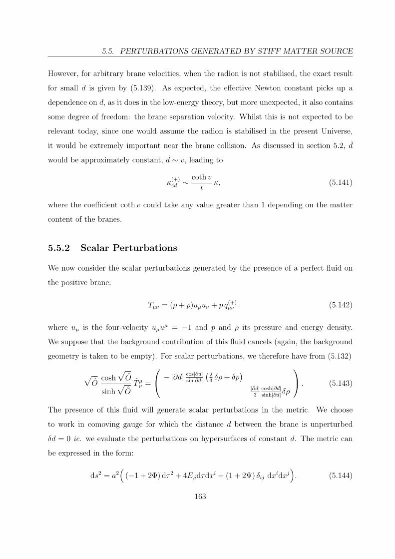
5.5. PERTURBATIONS GENERATED BY STIFF MATTER SOURCE
However, for arbitrary brane velocities, when the radion is not stabilised, the exact result
for small d is given by (5.139). As expected, the effective Newton constant picks up a
dependence on d, as it does in the low-energy theory, but more unexpected, it also contains
some degree of freedom: the brane separation velocity. Whilst this is not expected to be
relevant today, since one would assume the radion is stabilised in the present Universe,
it would be extremely important near the brane collision. As discussed in section 5.2, d
would be approximately constant, d ∼ v, leading to
κ(+)4d ∼
coth v
tκ, (5.141)
where the coefficient coth v could take any value greater than 1 depending on the matter
content of the branes.
5.5.2 Scalar Perturbations
We now consider the scalar perturbations generated by the presence of a perfect fluid on
the positive brane:
Tµν = (ρ + p)uµuν + p q(+)µν . (5.142)
where uµ is the four-velocity uµuµ = −1 and p and ρ its pressure and energy density.
We suppose that the background contribution of this fluid cancels (again, the background
geometry is taken to be empty). For scalar perturbations, we therefore have from (5.132)
√O
cosh√
O
sinh√
OT µ
ν =
− |∂d| cos|∂d|sin|∂d|
(23δρ + δp
)|∂d|3
cosh|∂d|sinh|∂d| δρ
. (5.143)
The presence of this fluid will generate scalar perturbations in the metric. We choose
to work in comoving gauge for which the distance d between the brane is unperturbed
δd = 0 ie. we evaluate the perturbations on hypersurfaces of constant d. The metric can
be expressed in the form:
ds2 = a2(
(−1 + 2Φ) dτ 2 + 4E,idτdxi + (1 + 2Ψ) δij dxidxj). (5.144)
163

CHAPTER 5. CLOSE-BRANE EFFECTIVE THEORY
In that gauge we then have:
δ |∂d| = dΦ. (5.145)
From the expression of the Ricci scalar (5.101), we get:
δR =κ
L(δρ− 3δp) . (5.146)
Working in terms of the conformal time (with ′ ≡ ∂τ ), we have a′′ = 0 for the background
(since we assumed the brane to be empty and spatially flat). Deriving the expression for
the perturbed Ricci tensor in (5.146), we have:
Ψ′′ +a′
a
(2k2 E + Φ′ + 3Ψ′)+
k2
3(2Ψ + 2E ′ − Φ) = a2 κ
6L(δρ− 3δp) . (5.147)
We now perturb (5.100), using for simplicity the notation
X(|∂d|) = |∂d| tanh(|∂d| /2)
Y (|∂d|) =1
|∂d|(tanh(|∂d| /2) + tan(|∂d| /2)) .
The ij (with i 6= j) component of the Einstein equation, to first order in the perturbations,
reduces to:
Φ−Ψ− 2E ′ =
(4a′
a+ 2
d′
d
)E, (5.148)
and the 0i-component to:
Ψ′ = −(
a′
a+
d′
2d
)Φ. (5.149)
So far these equations are equivalent to those one would have obtained in the low-energy
limit. The difference comes from the 00-component of the perturbed Einstein equations:
d′
dΦ′ +
a2
Ld
(2X − dX ′ + d3Y ′
)Φ− 2k2Ψ− a′
a
(6Ψ′ + 4k2E
)= −a
κ
6
d′
dcot d (2δρ + 3δp) , (5.150)
and from the equation of motion for d:
Φ′ +
(8d′a′2
LX +
a
L(Y ′d2 − 4X ′
)Φ + 3Ψ′ + 2k2E
= −aκ
6
(cot d (2δρ + 3δp)− 3 coth d δρ
). (5.151)
164

5.5. PERTURBATIONS GENERATED BY STIFF MATTER SOURCE
Note that one must, at this order, treat Φ,Φ′,Ψ and Ψ′ as four independent variables;
differentiation with respect to conformal time will miss terms arising from higher order in
d, since d and d′ are of different order. We must then solve the five equations (5.147-5.151)
simultaneously. Using (5.148) to eliminate Φ from (5.147), we obtain
4k2
(d′
d− a′
a
)E = 6 Ψ′′ + 2k2Ψ + 6
a′
a(Φ′ + 3Ψ′)− κ
La2 (δρ− 3δp) . (5.152)
We may use a combination of (5.150) and (5.151) to find an expression for Φ′ in terms
of Φ, Ψ, δρ and δp and hence write E in terms of Ψ, Ψ′, Ψ′′, δρ and δp. This can then be
used in (5.150) to obtain a complicated expression for Ψ in terms of Ψ′,Ψ′′,δρ and δp. We
then only keep the leading order in d for each coefficient, resulting in the much simplified
equation for the curvature perturbation on comoving hypersurfaces:
Ψ =
[− d′
d∂τ
]Ψ = −a2κ
6
d
dcoth d δρ, (5.153)
giving rise to the same relation between the four-dimensional Newtonian constant and the
five-dimensional one as in (5.139). Here again we may check that, apart from the mod-
ification of the effective Newtonian constant on the brane, the perturbations propagate
in the given background exactly the same way as they would if the theory was genuinely
four-dimensional. This is a very important result for the propagation of scalar pertur-
bations if they are to generate the observed large scale structure. The five-dimensional
nature of the theory does affect the background behaviour but on this given background
the perturbations behave exactly the same way as they would in the four-dimensional
theory.
This result is of course only true in the close-brane limit, for which the theory contains
no higher than second derivatives, only powers of first derivatives. When the branes are no
longer very close to each other, the theory will become higher-dimensional (in particular the
theory becomes non-local in the one-brane limit). The presence of these higher-derivative
corrections (not expressible as powers of first derivatives) is expected to modify the way
perturbations propagate in a given background, mainly because extra Cauchy data would
need to be specified, making the perturbations non adiabatic (Cf. chapter 4). However if
165

CHAPTER 5. CLOSE-BRANE EFFECTIVE THEORY
we consider a scenario for which the large scale structure is generated just after the brane
collision, the mechanism for the production of the scalar perturbations will be very similar
to the standard four-dimensional one.
5.5.3 Relation between the four- and five-dimensional Newto-
nian Constant
The relation (5.139) between κ(+)4d and the five-dimensional constant κ is formally only
valid for small distance between the branes. However if we consider the analysis of section
5.3.5, we may have some insights of what will happen if we had not stopped the expansion
to leading order in d. Here, terms of the form d d and more generally any term of the
form dnd(n+1) have been considered as negligible in comparison to d and therefore only the
terms of the form dn have been kept in the expansion. In a more general case, when the
branes are not assumed to be close to each other, any term of the form dn d(n+1) should be
considered and would affect the relation between the four-dimensional Newtonian constant
and the five-dimensional one. For moving branes, we therefore expect the relation between
κ(+)4d and κ to be:
κ(+)4d =
κ
LΩ
(d
L, d, d d, · · · , dn d(n+1)
). (5.154)
The relation is therefore a functional of d: Ω [d(t)] has an infinite number of independent
degree of freedom.
In the low-energy limit, or when the radion is stabilised, d ∼ d0 = const, the exact
expression of Ω is [121]:
Ω→ Ω [d(t) = d0] =ed0/L
2 sinh d0/L. (5.155)
For close branes, another limit is now known: When d L,
Ω [d L] =d
dcoth d. (5.156)
But in a general case, Ω (and therefore κ(+)4d ) is expected to be a completely dynamical
degree of freedom. For the present Universe the radion is supposed to be stabilised, but
in early-Universe cosmology, the effective four-dimensional Newton constant could be very
166

5.6. PERTURBATIONS IN THE PRESENCE OF A POTENTIAL
different from its present value. It might therefore be interesting to understand what the
constraints on such time-variation of the Newtonian constant would be and how it would
constrain the brane velocity [161], or whether such a time variation could act as a signature
for the presence of extra dimensions.
5.6 Perturbations in the Presence of a Potential
We now consider perturbations in the absence of matter on the branes when a potential for
the radion is present. As seen in section 2.8.1, the origin of this potential is not completely
understood but could be generated by the presence of bulk scalar fields in a mechanism
similar to the one proposed by Goldberger and Wise. For the purpose of this study however,
we shall not worry about its origin but introduce such a potential by hand directly in the
effective theory. This is similar to what has been done for the low-energy effective theory
(giving rise to the modified Einstein equation on the brane (2.85) and the Klein-Gordon
equation for the radion (2.86) ). The same procedure can now be applied to the theory in
the close-brane limit. For simplicity we will consider the branes to be empty. And work in
the positive tension brane frame, unless specified otherwise. The superscript (+) will be
omitted to lighten the notation.
5.6.1 Introduction of a Potential to Close-brane Effective Theory
We consider the addition of a potential in the close-brane theory by modifying the effective
stress-energy tensor for the radion in the Einstein equation (5.104):
T effµν =
1
d
[DµDνd +
2
Lg ∂µd∂νd− d Eµν −
( d +
z2g
L+
3f
L− d E + V (d)
)qµν
], (5.157)
where the potential V is related to the potential U introduced in the low-energy effective
theory by V (d) = 2d2/L U(φ(d)) in the close-brane limit. For this stress-energy to remain
conserved after the addition of the potential, the equation of motion of the scalar field
(5.105) has to be modified as well:
d = − 1
L
(2z2g + 4f
)+ d E + W, (5.158)
167

CHAPTER 5. CLOSE-BRANE EFFECTIVE THEORY
where the correction term W is a functional of the potential V (d) to be determined. The
modified Klein Gordon equation (5.158) should be consistent with the conservation of the
modified stress-energy tensor in (5.157). The divergence of T effµν can be calculated using the
constraint (5.108) for Eµν :
dDµTµ effν = ∂νd
[− V ′(d) +
3W + 4V
2d+
2g
L(3W + 2V )
+12
Lz2(f ′ + z2g′
)(V + W )
]+
1
L2O(d/L). (5.159)
To lowest order in d/L, we therefore need to modify the equation for the d with a term W :
W =2
3(dV ′(d)− 2V (d)) , (5.160)
where all covariant derivatives and index raising is taken with respect to q(+)µν . This is
precisely the same term which had to be introduced in the Klein Gordon equation (2.86)
in the effective low-energy theory, in the presence of a potential. Indeed, using the relation
between the potential U in (2.85) and the potential V in (5.157) for close branes, we have
V (d) = 2d2/L U(φ(d)) so W = 23(dV ′(d)− 2V (d)) = 4
3d3
LU,d which is the small d limit of
L2
6Ψ2 (1−Ψ2)3
U,d in (2.86). This procedure is completely consistent with the low-energy
theory and will give the same result to leading order in (∂d). In the absence of matter, the
scalar curvature does not vanish anymore but couples to the potential as
R = 2V ′(d). (5.161)
We have shown that it is therefore possible to modify the close-brane theory by intro-
ducing a potential in such a way that the conservation of energy and thus the Bianchi
identity remains unaffected. When no matter is present, it is therefore possible to extend
the close-brane theory in order to study the possibility of a potential for the radion. So
far no constraint has been imposed on the potential V (as long as its order of magnitude
is comparable with the other terms of the theory), however if V satisfies some slow-roll
or fast-roll conditions as explained in chapters 3 and 4, production of a scale invariant
spectrum might be possible. The inflaton could then have a natural physical interpreta-
tion as representing the distance between the branes. The five-dimensional nature of the
168

5.6. PERTURBATIONS IN THE PRESENCE OF A POTENTIAL
theory represents the key feature for the interpretation of the scalar field, it is therefore
essential to understand the higher-dimensional effects that such a scenario would have on
the production of a scale invariant spectrum. We suggest to study these effects (if any) in
the close-brane regime, where the effective theory on the brane seems genuinely different
from a standard theory of gravity in four-dimension.
5.6.2 Production of a Scale-invariant Power Spectrum in the
Close-brane Limit
Background behaviour
In order to study the perturbations in the close-brane theory with potential, we first con-
sider the background behaviour. For this we assume cosmological symmetry and consider
the positive tension brane to be spatially flat. Working in the conformally flat spacetime
ds2 = a2ηµνdxµdxν , (5.162)
in terms of the conformal time τ , the Ricci scalar (5.161) is
R = 6a′′
a3= 2V ′(d), (5.163)
and the equation of motion for the radion (that we will consider to play the role of the
radion) is given by (5.158):
d = −3Hd +1
L
(2d2g(z) + 4f(z)
)− 2
3(dV ′(d)− 2V (d)) , (5.164)
with z = d = d′
a. Using (5.163) and (5.164), the relation between the Hubble parameter
and the brane velocity in the presence of a potential is:
H2 =d
dL
(tanh
d
2− L H
)+
1
6dV. (5.165)
In the absence of a potential this was leading to the relation between H and d: LH =
tanh d2, but if the potential V is of the same order of magnitude than H or d (in particular
169

CHAPTER 5. CLOSE-BRANE EFFECTIVE THEORY
if V does not diverge at the collision, when d→ 0), this leads instead to
LH = tanhd
2+
L
6dV. (5.166)
As expected, the presence of the potential modifies the background behaviour. For ap-
propriate conditions on V , the Hubble parameter might evolve in such a way that the
production of a scale invariant spectrum in a contracting or expanding universe might be
possible. For a given potential, the background behaviour will be different than a stan-
dard four-dimensional one. However we do not concentrate on the specific constraints
the potential should have and we assume that it possible to tune the potential such that
the Hubble parameter satisfies the required background evolution. Instead, we consider
the propagation of perturbations on that given background and check whether the per-
turbations evolution for one given background is any different from the one in standard
four-dimensional gravity.
Scalar Perturbation
In order to study scalar perturbations, we work in comoving gauge for which δd = 0:
ds2 = a(τ)2 (ηµν + hµν) dxµdxν , (5.167)
with h00 = 2Φ, h0i = 2E,i and hij = 2Ψδij. In that gauge, the curvature perturbation on
comoving hypersurfaces is simply ζ = Ψ. Following the same procedure as in section 5.5.2,
we find the remarkably simple evolution equation for the curvature perturbation:
ζ ′′ +d′
dζ ′ + k2ζ = 0, (5.168)
where derivatives are performed with respect to the conformal time. The derivation of this
result does not need to be shown in detail as no main features differ from the derivation
of the scalar perturbations in section 5.5.2. However it is worth pointing out that the
derivation and the final result does not depend on the exact expression of the functions
f(z) and g(z).
170

5.6. PERTURBATIONS IN THE PRESENCE OF A POTENTIAL
This is a remarkable result which is surprisingly similar to what would be obtained in
standard four-dimensional gravity with a scalar field. We have already pointed out that
in the effective low-energy theory, the scale factor a in the Einstein frame is related to the
scale factor in the positive tension brane frame by: a =√
2dL
a, so that d′
d≈ 2 a′
a, which in
the small d limit corresponds exactly with what we have from a four-dimensional theory:
ζ ′′ + 2a′
aζ ′ + k2ζ = 0. (5.169)
This seems to suggest that the curvature propagation will not be affected by the five-
dimensional nature of the theory in the close-brane limit.
Consequences for brane inflation
In the context of inflation, if the potential V is such that the Hubble parameter satis-
fies slow-roll conditions, or more specifically if the potential is such that a′
a∼ τ−1, ie.
a ∼ −(Hτ)−1, the curvature perturbation will evolve following the same behaviour as
in standard inflation and will therefore generate a scale invariant power spectrum which
could be responsible for the present large scale structure. On the down side, using the
close-brane theory, it seems difficult to track any characteristic signature of such a brane
inflation model in the large scale structure. One of the reason why the resulting perturba-
tion evolution seems to be so similar to a normal evolution comes from the fact that the
close-brane theory differs by the presence of higher-order derivatives terms which can all
be expressed as a function of |∂d|. As it is always possible to work in a gauge for which
|∂d| is unperturbed, only the background will be strongly affected by the presence of this
functions. At the perturbed level, on the other hand, the differences from standard four-
dimensional gravity can always be reinterpreted as background effects. So by modifying the
background behaviour, the evolution of the perturbations will appear unaffected. This is
however only valid to leading order in d/L where terms of the form d ∂µ∂νd are considered
to be negligible in comparison to ∂µd ∂νd. When the theory is genuinely of higher order in
derivative ie. including terms which can not be expressed in terms of first or second order
derivative, this result might not hold any longer. However we have seen in chapter 4, that
171

CHAPTER 5. CLOSE-BRANE EFFECTIVE THEORY
the presence of quadratic terms in the Weyl tensor, (which are genuinely higher order in
derivatives) did not seem to affect brane inflation, but could on the other hand affect the
production of a scale invariant spectrum in a fast-roll potential.
Consequences for a fast-roll potential
It is worth pointing out that the result in (5.169) corresponds exactly with the result used
in a number of work [90, 91] and in particular by P. Creminelli et. al. in [156]. Their
argument is therefore completely valid. In particular they show that for an expanding
universe with slow-roll constraints on the background behaviour, there will be production
of a scale invariant spectrum. We have shown here that the five-dimensional nature of
the theory does not affect the result provided the large scale structure is produced in a
regime where the branes are very close to each other. On the other hand, in the case of a
fast-roll background behaviour, which necessities a contracting universe, no scale invariant
spectrum seems to be observable. The reason why there seems to be production of a
scale-invariant spectrum as shown in the previous chapter, section 4.3.3, seems to be a
gauge artifact. In section 4.3.3, we have indeed worked in Newtonian gauge, for which
the variable u in eq.(4.57) seems to acquire a scale invariant growing mode. However,
as shown in [156], this is due to the fact that the wrong variable is used to study the
power spectrum. Working in terms of the curvature perturbation in comoving gauge, the
propagation evolution satisfies (5.169) which generates a scale invariant power spectrum
only if a ∼ τ−1 and therefore does not produce any scale invariant power spectrum in the
fast-roll contracting case for which a ∼ τ 2εF /(1−2εF ), where εF 1. Their argument was
relying on the fact that a four-dimensional theory was valid to study the evolution of the
curvature perturbation, which could be contestable. But we have shown here that this is
indeed the case, if the branes are close enough to each other. We can therefore argue that
their result would be reliable in that case and no scale invariant power spectrum seems to
be produced in such a fast-roll scenario.
This conclusion can appear to be in contradiction with the one of [154], where they con-
172

5.7. FIRST KALUZA KLEIN MODE IN THE CLOSE-BRANE LIMIT
clude that a scale invariant can indeed be produced in this scenario using five-dimensional
arguments. We can however point out that their result was relying strongly on the validity
of the moduli space approximation, or low-energy effective theory, which we have shown
to be valid only to second order in velocity. Their result, however predicts the production
of a scale invariant power spectrum with coefficients to fourth order in velocities, which
appears to be much beyond the regime of validity of the moduli-space approximation, and
therefore can not be entirely trusted.
To finish this chapter on close-brane theory, we shall end up by giving in next the section
an extra argument confirming that the terms included in chapter 4 are indeed generic to
braneworld cosmology and can be interpreted as part of the first Kaluza Klein modes.
5.7 First Kaluza Klein Mode in the Close-brane Limit
We now work with the same philosophy as [112] in order to find the next to leading order
term in the low-energy effective theory of section 2.6, and see in particular if, in the close-
brane limit, it is possible to work out the covariant expression of the first KK mode as
derived in the quasi-static limit in section 2.7. For this we consider matter on the positive
tension brane only.
In order to find the contribution of the Weyl tensor Eµν for the zero mode (given by the
low-energy effective theory in (2.46)) as well as the first KK mode, we may use the same
technique as before which is to expand the extrinsic curvature on the negative brane as a
Taylor series around the positive brane
K(−) µ
ν −K(+) µ
ν =κ
2T µ
ν = ∂yK(+) µ
ν +1
2∂2
yK(+) µ
ν +1
6∂3
yK(+) µ
ν + · · · , (5.170)
where T µν is associated to the stress-energy tensor of matter on the positive tension brane
and the first equality is a consequence of the Israel matching conditions (5.90) and (5.91).
For simplicity, we will work in what follows in a low-energy limit, where the quadratic (and
cubic) terms in the stress-energy tensor can be neglected as well as the coupling of matter
with the radion. Furthermore we assume that we can work in a gauge (5.27) where the
173

CHAPTER 5. CLOSE-BRANE EFFECTIVE THEORY
branes are static and for which A, the yy-component of the metric, can be considered to
be independent of y. In that case, using the evolution equations for the extrinsic curvature
(2.5) and the Weyl tensor (2.33) are
∂yKµν = −dEµ
ν −DµDνd− dKµαKα
ν +d
L2δµ
ν (5.171)
∂yEµν = 2dKα
ν Eµα − d
3
2KEµ
ν −d
2Kα
β Eβαδµ
ν + d UKµν + d(K3)µ
ν (5.172)
−∂αd [DµKαν + DνKµα − 2DαKµ
ν ] .
where again (K3)µν are some cubic terms in the traceless part of the extrinsic curvature
and the operator U is such that for any tensor Zµν ,
UZµν = Cµ
ανβZαβ − 1
2[DαDµZα
ν + DαDνZαµ − 2Zµ
ν ] . (5.173)
We can now differentiate the extrinsic curvature to third order, using the relations (5.171)
and (5.172) and neglecting any term of the form ∂d T or any higher order in T . We find
the following relations evaluated on the positive brane:
∂yK(+) µ
ν = −dEµν(0)−DµDνd +
2d
LκT µ
ν (5.174)
∂2yK
(+) µν = d2 χµ
ν(0)− 4d
LDµDνd−
2
L∂µd∂νd +
1
L(∂d)2 δµ
ν −6d2
LEµ
ν(0) (5.175)
∂3yK
(+) µν =
d3
L3Bµ
ν +d3
L2hEµ
ν(0) +d3
L3g(E2(0)
)µν, (5.176)
with χµν (0) = −κ
2U T µ
ν − 2 κL2 T µ
ν and h = L2 U − 28. By (E2(0))µν we designate quadratic
term in the Weyl tensor on which the operator g acts. The exact action of g is not necessary
as it is negligible at low-energy. The tensor Bµν can be expressed in terms of the radion
and the extrinsic curvature and does not depend explicitly on Eµν , for this study we do not
need to compute its exact expression.
Using these expressions in the Taylor expansion (5.170) to third order in d, we therefore
get the equation for Eµν :
d(1 + 3d
L− d2
6L2h)Eµ
ν(0) =κ
2(1 + 2
d
L)T µ
ν +d2
2χµ
ν(0) (5.177)
−DµDνd− 2d
LDµDνd−
1
L
(∂µd∂νd−
1
2(∂d)2δµ
ν
),
174

5.7. FIRST KALUZA KLEIN MODE IN THE CLOSE-BRANE LIMIT
where we have omitted terms coming from higher derivatives of the extrinsic curvature
and terms that are negligible at low-energy. If we consider the Weyl tensor to be of the
form Eµν = Eeff µ
ν +EKK µν where Eeff µ
ν is the Weyl tensor derived in the low-energy effective
theory (2.46), which corresponds to the zero mode in section 2.7. The KK modes should
thus be encoded in EKK µν . Substituting this expression back into the equation (5.177) for
Eµν we get:
EKK µν = −κ
6d UT µ
ν , (5.178)
which should correspond to the first KK mode at low-energy, and to lowest order in d.
We may now compare this result with what is found in the quasi-static limit. We
have shown in section 4.2.1, that in the quasi-static limit, the first KK mode was correctly
reproduced by the term 11−Ψ2 E
corrµν with
Ecorrµν = αL2Aµν , (5.179)
and α = 2d3
3L3 + O( d4
L4 ). Where the tensor Aµν was the one derived from the action∫dx4√−q C2, given in (4.4) or (4.6). When the evolution of the radion is negligible,
we indeed have, to linear order, the standard Einstein equation on the brane Rµν =
κL
11−Ψ2
(Tµν − 1
2Tqµν
), so we have Tµν ≈ 2d
κ
(Rµν − 1
6Rqµν
). Substituting this into the
expression (5.178) for the first KK mode, we therefore have:
EKK µν = −d2
3d U
(Rµ
ν −1
6Rδµ
ν
)= −d2
3Cµ
ανβRαβ +d2
6[DαDµRα
ν + DαDνRαµ − 2Rµ
ν ] (5.180)
− d2
18[DµDνR− 2Rδµ
ν ] .
Decomposing the Weyl tensor Cµανβ in terms of the Riemann tensor, the Ricci tensor of
the scalar curvature, and using the fact that DαDµRαν = 1
2DµDνR + Rµ
αRαν − Rµ
ανβRαβ,
we obtain:
EKK µν = −d2
3
[2Rµ
ανβRαβ + Rµν −
1
3DµDνR−
1
6Rδµ
ν (5.181)
+1
6R2δµ
ν −2
3RRµ
ν −1
2RαβRαβδµ
ν
],
175

CHAPTER 5. CLOSE-BRANE EFFECTIVE THEORY
which corresponds precisely to the tensor Aµν we took as an ansatz for the first KK mode
in section 4.2.1:
EKKµν =
d2
3Aµν =
1
1−Ψ2Ecorr
µν . (5.182)
This is therefore a strong argument confirming that the ansatz we took in chapter 4 to
model part of the first KK mode is consistent with the five-dimensional covariant derivation
of this mode. In particular in the section 4.3.3, we worked in a low-energy regime and
studied the effect of this mode in the duality between fast-roll and slow-roll. For that
low-energy study, this derivation confirms the validity of our ansatz and therefore the
conclusion that were drawn on that section. In a more general case, however the term
EKK µν = −κ
6d UT µ
ν should be considered as representing part of the first KK mode in the
close-brane limit.
5.8 Discussion
In the first part of this chapter we pointed out the discrepancy between predictions from the
effective four-dimensional low-energy theory and the exact five-dimensional results. The
difference has been established in the regime where the branes were close and all through
this paper we worked to leading order in d/L.
In order to go beyond the low-energy effective theory, we established a formalism to
find the electric part Eµν of the five-dimensional Weyl tensor on both branes. This tensor
represents the only quantity which is unknown from a four-dimensional point of view as
it encodes information about the bulk geometry. Finding its expression on the brane
is therefore the key element in order to study the geometry of a brane within an extra
dimension.
Using this formalism in the small distance limit, we found an exact expression for the
Weyl tensor on each brane, valid at leading order in d/L but at all orders in velocities, or
for any energy scale. We were therefore able to modify the regime of validity of the effective
theory from a low-energy regime valid independently of the branes distance to a regime
176

5.8. DISCUSSION
valid at all energy scales for close branes. This regime of validity is relevant for cosmology
since it represents one of the main focus of present braneworld models. Understanding the
behaviour of branes just before or just after a collision is indeed crucial if our Universe
emerged from a brane collision. If the Big Bang were initiated by such a collision, it is
consistent to assume that the large scale structure was produced in a regime where both
branes were close. Even if this regime is not valid after a while, effects that originated
during this period are unlikely to be eliminated once the branes are far apart and the fifth
dimension has opened up, leaving the possibility of exciting the Kaluza Klein modes.
Keeping this objective in mind, we established a theory that allows us to study such
scenarios and have checked the consistency of its predictions for homogeneous and isotropic
geometries. We argue that this theory is remarkably straight-forward to use since it includes
only four-dimensional quantities and is effectively second order in derivatives, the only
higher-order corrections coming as powers of first derivatives. This feature will facilitate
any comparison with other four-dimensional theories. It is worth pointing out that it is
different from other higher-derivative theories [150,162] in that it is not derived using the
assumption that it can be derived from an action, and it is different from a theory relying
on purely string effects [81, 163, 164]. Already for the background, an interesting result
can be pointed out: when the branes are empty the Hubble parameter on each brane is
bounded by L2H2 < 1, which could not have been derived from the low-energy effective
theory, although this does not hold anymore when some matter is introduced on the branes
or if a potential is added for the radion. Another interesting result of the theory is that the
expansion seems to break down when the velocities are of order |∂d| ∼ π. However when
any physical quantity is calculated (for the background as much as for perturbations), the
terms of the form sin |∂d|−1 do not contribute and the result is limited by any value of |∂d|.
We can then use this close-brane effective theory in order to understand the way matter
and the radion couples to gravity at the perturbed level. In order to do so, we considered
a scenario in the stiff source approximation for which the background is supposed to be
unaffected by the presence of matter and considered the production of curvature and tensor
perturbation sourced by the presence of matter fields on the brane. Although the five-
177

CHAPTER 5. CLOSE-BRANE EFFECTIVE THEORY
dimensional nature of the theory does affect the background behaviour, we have shown
that for a given background the perturbations propagate the same way as they would in a
standard four-dimensional theory. This is only true in the limit of small brane separation
and is not expected to be valid outside this regime. However, since the large scale structure
of the Universe might have been produced in a period for which the branes could have been
close together (for instance just after a brane collision initiating the Big Bang), this regime
is of special interest. The fact that the perturbations behave the same way, for a given
background, as they would in a four-dimensional theory is a remarkable result for the
production of the large scale structure which could be almost unaffected by the presence
of the fifth dimension. This is true for an inflationary scenario. On the other hand in a
fast-roll scenario, this confirms the fact that no scale invariant power spectrum seems to
be produced. This is however only valid if we consider the perturbations to be generated
in a regime where the branes are close enough.
The relation between the four-dimensional Newtonian constant and the five-dimensional
one is however affected by the expansion of the fifth-dimension. As we have shown in the
Introduction of this thesis and in chapter 2, as well as in [50, 121], the four-dimensional
Newtonian constant is dependent on the distance between the branes, giving a possible
explanation of the hierarchy problem. In this chapter, we have shown that the four-
dimensional Newtonian constant also has some dependence on the brane velocity which
we computed exactly in the small-distance limit. This might provide us with an obser-
vational signature for the presence of extra dimensions. Outside the small d regime, we
expect the four-dimensional Newtonian constant to depend on the five-dimensional one
not only through the brane separation velocity d but also on higher derivatives of the dis-
tance between the branes d(n), making the requirement for moduli stabilisation even more
fundamental for any realistic cosmological setup within braneworld cosmology.
178

Chapter 6
Conclusions
Ah Puch, the Underworld (Maya)
We end by summarising in this chapter the main points of this thesis. As we shall see,
there are several criticisms that can be made either of the formalism developed or of the
validity of the results. We shall therefore emphasise possible extensions of this work, and
show how some potential problems might be cured.
6.1 Objective
The notion of low-energy effective field theories has become a familiar concept in particle
physics. In these theories, the influence of higher energy degrees of freedom (or equivalently
higher dimensional ones) is described by the addition of higher derivative or mass terms
179

CHAPTER 6. CONCLUSIONS
(irrelevant operators) in the effective action. These can be obtained by explicitly integrating
out the high energy modes. This approach is valid as long as the energy scales of interest
are much less than the energy scales of the modes which have been integrated out (ie.
when these modes are very massive).
In this thesis, the approach is philosophically distinct: We have attempted to model
the five-dimensional effects in four-dimensional terms, in regimes where the energy scales
of interest are comparable to the five-dimensional energy scales. In these regimes, the
traditional four-dimensional low-energy effective field theory approach will thus not be
valid. By making various simplifying assumptions in distinct cases, we have nevertheless
been able to model the five-dimensional effects with a four-dimensional theory, although
this often may not be describable in terms of an action.
6.2 What did we learn ?
Although not every step of this thesis is fundamentally new, the general analysis has led
to several results or concepts which are worth emphasising one last time:
Braneworld cosmology is well described by an effective theory at low energies,
but is genuinely different at high energies. The modified Einstein equation on an orb-
ifold brane presents two characteristic terms. First gravity couples quadratically to
the stress-energy tensor of matter on the brane. Secondly, Kaluza Klein modes, repre-
senting excitations from the bulk degrees of freedom, are present on the brane. These
two elements (which disappear at low energies), reflect the genuinely five-dimensional
nature of the theory, and hence the necessity of going beyond the low-energy descrip-
tion.
The low-energy effective theory breaks down at large-velocities, even for the back-
ground where it could be believed to give an accurate result to all orders. This
discrepancy is indeed independent of the Kaluza Klein modes observed at the per-
turbed level in the quasi-static limit and of the quadratic terms in the stress-energy.
180

6.2. WHAT DID WE LEARN ?
It reflects the fact that the integration constant (arising from integration of the Ein-
stein equation), is related to the radion dynamics (or in a more general system, to
the moduli dynamics). The relation predicted by the low-energy effective theory is
shown to be only valid at low velocities and to break down at second order.
To go beyond the low-energy limit, the zero mode can be correctly modelled using
an adiabatic argument together with a conformal assumption. Using this assumption,
we explore the possibility for the branes to be conformal to each other. In such a
case a homogeneous tensor which vanishes for the background can be separated out
from the Weyl tensor. Since scalar perturbations of a conserved fluid follow their
background behaviour in an adiabatic regime, this homogeneous part of the Weyl
tensor can be neglected as a first approximation.
In this model, Kaluza Klein modes, which break the conformal assumption, can be
introduced as corrections to the homogeneous part of the Weyl tensor. By consider-
ing different corrections on each brane, the conformal assumption is hence relaxed.
The treatment allows the study of Kaluza Klein type of modification to the brane
geometry.
In the quasi-static limit, the first Kaluza Klein mode can be modelled by a four-
dimensional local tensor. This term can be derived from an action containing quadratic
terms in the four-dimensional Weyl tensor. The first Kaluza Klein mode can be mod-
elled by the presence of this new term which is introduced with different coefficients
on each brane. This model gives an exact result only in the quasi-static limit, and one
can argue that in a general setup, this result should not be valid. However, it is very
unlikely that its contribution could be cancelled out in generic situations. Although
in general situations, the term we have considered might not be the more significant
one, it should still be present in a wide range of scenarios. This term might hence be
present and have an affect beyond the quasi-static limit.
In the close-brane regime, a four-dimensional effective theory can be derived. By
181

CHAPTER 6. CONCLUSIONS
successive integration of the bulk equations of motion, the induced Einstein equa-
tion of the brane can be expressed covariantly and in a closed form. The resulting
theory contains terms of higher orders in derivatives although they can actually be
expressed as a power of first derivative terms. The Cauchy data to be specified in
the initial conditions of the theory is hence the same as for a genuinely second order
theory, there is no need for new information to be specified. Although it appears
effectively four-dimensional, this theory precisely models five-dimensional effects of
the theory and gives precisely the exact result for the background in the close-brane
regime. It can as well be seen as a generalisation of the well-known low-energy four-
dimensional effective theory in the close-brane limit and is hence an extension of this
theory beyond the low-energy approximation.
Using these results, and the different modelling theories, signatures in the propagation
of perturbations are shown to be very weak. Indeed, when the inflaton scalar
field lives on the brane, corrections to standard four-dimensional chaotic inflation
come at second order in the slow-roll parameters. The main differences arise from
the background behaviour, which can always be remodelled by a change of variables.
Such background differences lead to a possible reinterpretation of the potential. The
constraints to apply on the potential are hence different, and in particular a scenario
for steep inflation, for which the potential is not flat, is possible.
Furthermore, perturbations produced in a regime where the branes are close enough
follow a general four-dimensional behaviour, although the underlying theory is gen-
uinely different from four-dimensional scenarios. We can hence conclude that the
four-dimensional treatment is usually acceptable in an adiabatic situation and gives
accurate predictions.
The presence of a shear tensor can however be pointed out at high energies when the
inflaton lives on the brane. This anisotropic term is usually absent in standard chaotic
inflation and hence is interesting to study in braneworld inflation. Unfortunately, it
does not provide any observational signatures which could characterise braneworld
182

6.2. WHAT DID WE LEARN ?
scenarios.
On the other hand, higher-order derivative corrections modify the way perturba-
tions propagate. When correction terms that could model Kaluza Klein corrections
are taken into account, the behaviour of perturbations is genuinely different. In par-
ticular, perturbations propagate with a speed of sound slightly different from the
speed of light, which is not necessarily the same for tensor and scalar perturbations.
Another interesting difference arises in the estimate of the non-gaussianity. Although
it remains small in our analysis, it does not appear to be damped by the slow-roll
parameters. It hence opens up the possibility for the non-gaussianity to be relatively
large in a general braneworld scenario.
In the case of this study, the corrections are considered to be small and do not
affect the general features of inflation. The differences are not important enough to
create an observable distinction to inflation. However, for perturbations evolving in
a fast-roll potential, the production of a scale invariant power spectrum is in general
affected and the slow-roll/fast-roll duality is hence broken.
A general bulk brane has an induced Einstein equation which presents different re-
markable elements, not present on an orbifold brane. The presence of these terms
is related to the degrees of freedom present on the brane and not fixed by the Z2-
reflection symmetry. At high energies, the coupling to matter is very different from
what is usually expected from four-dimensional theories. Their study is of special
interest, as their behaviour is closer to usual D-branes (putting aside the charges and
form fields), and hence their study can lead to interesting features for these branes as
well. When an adiabatic regime is considered, an effective four-dimensional theory
can be derived on such branes, provided no matter fields are introduced. The way
to derive this theory is very similar to what has been done for orbifold branes and
general Kaluza Klein type of corrections could be considered as well.
183

CHAPTER 6. CONCLUSIONS
6.3 Criticisms and Going forward
Although we believe the previous development to be formally correct, different criticisms
can be made. We shall summarise them in what follows and see what alternatives can be
proposed to extend the study. Such an extension could give rise to more interesting results.
The different points one might criticise are the followings:
The treatment of the Weyl tensor. In chapters 3 and 4, the treatment of the Weyl
tensor has been imposed by hand at each steps, instead of being inferred by solving
the five-dimensional equations of motion like the more coherent procedure which is
followed in 5. The treatment of chapters 3 and 4 does go beyond the usual assump-
tions, where the Weyl tensor is often simply neglected [129, 139, 144] or treated as
radiation [165], but despite this fact, the way the homogeneous part of the Weyl ten-
sor is treated is still far from an exact analysis. Part of its behaviour, is only guessed
in chapter 4 and an ansatz is put by hand. This extends the treatment of [162], for
instance, which assumed the presence of some generic terms in the action, without
constraining these terms with the known background behaviour, nor the quasi-static
limit, or any other well defined and computable regime.
The treatment of chapter 5, on the other hand presents a better way to attack the
problem, in a more five-dimensional way. In particular, the last section shows how
the ansatz of chapter 4 can be incorporated in a more general calculation. We believe
this is a better way to treat the problem, and further works in this direction should
bring better insight on the behaviour of the Weyl tensor.
The one-brane limit has been considered in chapters 3 and 4. In this limit, the negative
tension brane decouples from the positive one and the study could hence be focused
on the quadratic terms in the stress-energy tensor on the brane or on Kaluza Klein
corrections, without needing to include the backreaction of the negative brane. But
in the one-brane limit of the RS model, the notion of a discrete Kaluza Klein tower
has to be replaced by a Kaluza Klein continuum. There is hence no real sense in
184

6.3. CRITICISMS AND GOING FORWARD
considering the first Kaluza Klein mode and its effect in that model. However this
does not mean that corrections are not present, (Kaluza Klein effects are expected
to be more important in the one-brane limit). In particular if the correction term
we have considered affects the brane geometry in some limit, it is unlikely that other
terms present in the Kaluza Klein continuum will cancel this effect.
In chapter 4, the correction term modelling the first Kaluza Klein mode was
assumed to be small, and hence no real conclusive remarks could be clearly made.
This assumption was made because the correction generates a term of fourth order
in derivatives. It is hence difficult to understand how initial conditions should be
imposed and to solve the equations exactly. We may stress that this problem does
not exist in other higher-derivative theories such as in [81] or in theories including
Gauss-Bonnet terms [85], since the higher-derivative terms are expressible as powers
of first or second order derivatives.
This problem could be solved if the equations were solved numerically and if the
usual Bunch-Davis vacuum was still considered as the initial condition. Assuming
this vacuum was still valid at higher order in derivatives, initial conditions could
hence be imposed after differentiation of the Bunch-Davis vacuum. By using such a
method, it would be possible to go beyond the small correction assumption, and hence
consider the entire effect of this term. This should lead to much more interesting and
conclusive remarks.
Only a first order expansion in brane separation has been considered in the close-
brane theory. Although the first order expansion has been remarkably simple and
straight-forward to work with, it has not led to any features that could not be ob-
tained from a four-dimensional scenario. However, if we go beyond the first order,
some genuinely higher-order derivative terms will appear and affect the behaviour of
perturbations in a non-trivial way. Studying the next to leading order terms in the
close-brane effective theory would hence be a natural extension to consider.
185

CHAPTER 6. CONCLUSIONS
No mechanism has been suggested to explain the presence of a potential. Such
a potential is indeed needed either for inflation or to generate a scale-invariant power
spectrum, but has not been derived from any theory. In chapters 3 and 4, inflation
was considered on the brane where an inflaton scalar field was supposed to live. In
that case, the problem is the same as for usual four-dimensional inflation: The origin
of the inflaton scalar field is unknown and we only assume the existence of a potential
satisfying some slow-roll constraints. In chapter 5, the radion plays the role of the
inflaton, but the potential is introduced by hand in the effective theory. In order
to take this model seriously, one should suggest a mechanism for the production of
such a potential, relying on higher-dimensional features, such as the Goldberger-Wise
mechanism [122], or on properties of the underlying theory such as the one considered
for brane inflation, as explained in the introduction.
We have focused our study on unrealistic models. The Randall Sundrum model is
indeed nothing else but a toy model, in which some of the higher-dimensional prop-
erties can be explored. However, it seems absolutely necessary to incorporate these
effects in more realistic scenarios emerging from string/M-theory. These scenarios
will in general contain D-branes, which are much more complicated objects than
orbifold branes. Not only are they not submitted to any reflection symmetry, but
their physics is much richer due to the presence of gauge fields which have here been
neglected. The extension of the study in this thesis to more realistic and richer
scenarios is hence the real objective one should aim at.
This thesis is therefore only a small step in the study of cosmological signatures of
braneworld cosmology. Due to the nature of the toy model we concentrated on, and because
of the approximations we have made, the conclusion can only be limited. However, it has
allowed us to develop different ways to attack the problem depending on which specific
regime we are interested in. Understanding the problem as a whole is a very difficult task
to address, but we have attempted to decompose it in small, better defined questions. For
these specific questions, a set of tools has been developed which can then be used in more
186
6.3. CRITICISMS AND GOING FORWARD
sophisticated situations. Applied to the RS toy models, not many new physical results can
be expected, but we hope that the way of approaching the problem can be extended to
more realistic scenarios where the physical implications would be richer.
187

CHAPTER 6. CONCLUSIONS
188

Appendix A
Covariant study of an empty bulk
brane
In this appendix, we apply the same formalism as in section 3.2.1, in order to model the
RS model in presence of a bulk brane as described in section 2.8.2. In particular, we start
with the similar assumption that all branes may be treated as conformal to each other:
q(±)µν = X(±) 2q(b)
µν (A.1)
where we use the same notation as in section 2.8.2: the superscripts (±) designate the
positive and negative boundary branes and quantities referring to the bulk brane are la-
belled with the index (b). Although this conformal assumption is not valid in general, we
expect it to remain valid for long wavelength adiabatic perturbations, and in chapter 4,
we explain how this conformal assumption may be broken for the usual RS scenario. The
same procedure could be used to extend the bulk brane treatment that we shall explain in
what follows.
In what follows we consider matter to be present only on the boundary branes, the
bulk brane being empty. We will use the same notation as in section 3.2.1 and work in
the bulk brane frame. Therefore all covariant derivatives and indices raising will be taken
with respect to q(b)µν unless specified otherwise. Considering the equation of motion (3.3) of
the conformal factor in the two-branes model, the fields X and Y can be shown to satisfy
189

APPENDIX A. COVARIANT STUDY OF AN EMPTY BULK BRANE
the analogous equation of motion:
X(±) =1
6
(R(b) −X2Π(±)
)X(±) (A.2)
where Π(±) are defined in section 3.2.1. For empty boundary branes, we may point out
that X and Y are conformally invariant with respect of the bulk brane.
The procedure used in section 3.2.1 in order to express the Weyl tensor covariantly as
in (3.25) may be followed exactly the same way here. There are now two traceless and
conserved pseudo-stress-energy tensor TX,Y effµν defined the same way as in (3.21 - 3.23):
TX(±) effµν = G(2)
µν X(±) 2 + 4 ∂µX(±) ∂νX
(±) − 2X(±)DµDνX(±) (A.3)
+q(b)µν
(2X(±)X(±) −
(∂X(±)
)2) −X(±) 2Π(±)µν + E (±)
µν
q(b)µνTX(±) effµν = 0 (A.4)
DµTX(±) eff µ
ν= 0 (A.5)
where E (±)µν satisfy the equation (3.18), (3.19). For the background, following the procedure
of section 2.8.2, the induced Weyl tensors on each brane give rise to the dark energy terms
in the modified Friedmann equations (2.93):
E(+) i
j = −1
3E
(+) 00δ
ij = −CL
L2L
1
a4+
δij (A.6)
E(−) i
j = −1
3E
(−) 00δ
ij = −CR
L2R
1
a4−
δij (A.7)
E(b) i
j = −1
3E
(b) 00δ
ij = − CRLL − CLLR
LLLR (LR − LL)
1
a4b
δij, (A.8)
where we have considered the bulk brane to be empty. In the background, the induced
Weyl tensor on each brane are therefore related as follows:
E(b)µν =
LL
LL − LR
X(+) 2 E(+)µν +
LR
LR − LL
X(−) 2 E(−)µν . (A.9)
By analogy to (3.5), we construct the traceless quantity ∆Eµν that vanishes in the back-
ground:
∆Eµν =
(− LL
LL − LR
X(+) 2 Π(+)µν −
LR
LR − LL
X(−) 2 Π(−)µν
)(A.10)
−(
R(b)µν −
LL
LL − LR
X(+) 2 R(+)µν −
LR
LR − LL
X(−) 2 R(−)µν
).
190
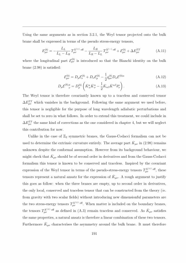
Using the same arguments as in section 3.2.1, the Weyl tensor projected onto the bulk
brane shall be expressed in terms of the pseudo stress-energy tensors,
E(b)µν = − LL
LL − LR
TX(+) effµν − LR
LR − LL
TX(−) effµν + E (b)
µν + ∆ETTµν (A.11)
where the longitudinal part E (b)µν is introduced so that the Bianchi identity on the bulk
brane (2.98) is satisfied:
E (b)µν = DµE (b)
ν + DνE (b)µ −
1
2q(b)µν DαE (b)α (A.12)
DµE (b) µν = D(b)
µ
(Kµ
αKαν −
1
2KαβKαβδµ
ν
). (A.13)
The Weyl tensor is therefore covariantly known up to a traceless and conserved tensor
∆ETTµν which vanishes in the background. Following the same argument we used before,
this tensor is negligible for the purpose of long wavelength adiabatic perturbations and
shall be set to zero in what follows. In order to extend this treatment, we could include in
∆ETTµν the same kind of corrections as the one considered in chapter 4, but we will neglect
this contribution for now.
Unlike in the case of Z2 symmetric branes, the Gauss-Codacci formalism can not be
used to determine the extrinsic curvature entirely. The average part Kµν in (2.98) remains
unknown despite the conformal assumption. However from its background behaviour, we
might check that Kµν should be of second order in derivatives and from the Gauss-Codacci
formalism this tensor is known to be conserved and traceless. Inspired by the covariant
expression of the Weyl tensor in terms of the pseudo-stress-energy tensors TX(±) effµν , these
tensors represent a natural ansatz for the expression of Kµν . A rough argument to justify
this goes as follow: when the three branes are empty, up to second order in derivatives,
the only local, conserved and traceless tensor that can be constructed from the theory (ie.
from gravity with two scalar fields) without introducing new dimensionful parameters are
the two stress-energy tensors TX(±) effµν . When matter is included on the boundary branes,
the tensors TX(±) effµν as defined in (A.3) remain traceless and conserved. As Kµν satisfies
the same properties, a natural ansatz is therefore a linear combination of these two tensors.
Furthermore Kµν characterises the asymmetry around the bulk brane. It must therefore
191
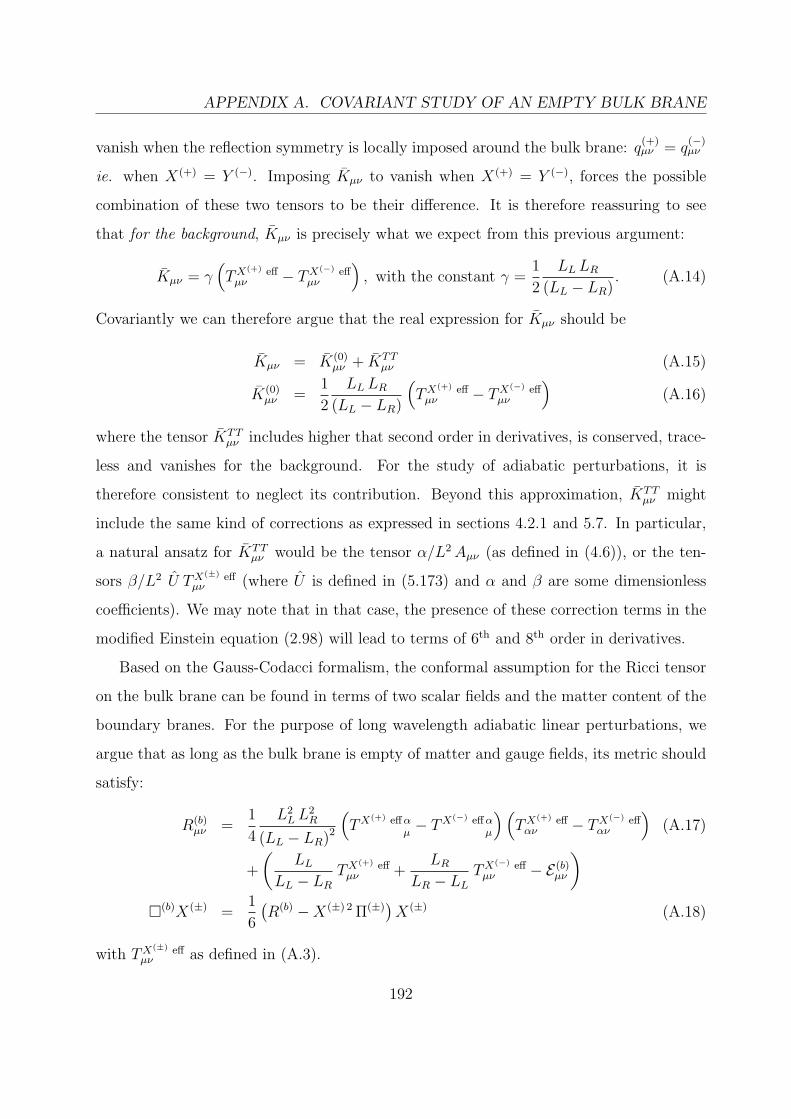
APPENDIX A. COVARIANT STUDY OF AN EMPTY BULK BRANE
vanish when the reflection symmetry is locally imposed around the bulk brane: q(+)µν = q
(−)µν
ie. when X(+) = Y (−). Imposing Kµν to vanish when X(+) = Y (−), forces the possible
combination of these two tensors to be their difference. It is therefore reassuring to see
that for the background, Kµν is precisely what we expect from this previous argument:
Kµν = γ(TX(+) eff
µν − TX(−) effµν
), with the constant γ =
1
2
LL LR
(LL − LR). (A.14)
Covariantly we can therefore argue that the real expression for Kµν should be
Kµν = K(0)µν + KTT
µν (A.15)
K(0)µν =
1
2
LL LR
(LL − LR)
(TX(+) eff
µν − TX(−) effµν
)(A.16)
where the tensor KTTµν includes higher that second order in derivatives, is conserved, trace-
less and vanishes for the background. For the study of adiabatic perturbations, it is
therefore consistent to neglect its contribution. Beyond this approximation, KTTµν might
include the same kind of corrections as expressed in sections 4.2.1 and 5.7. In particular,
a natural ansatz for KTTµν would be the tensor α/L2 Aµν (as defined in (4.6)), or the ten-
sors β/L2 U TX(±) effµν (where U is defined in (5.173) and α and β are some dimensionless
coefficients). We may note that in that case, the presence of these correction terms in the
modified Einstein equation (2.98) will lead to terms of 6th and 8th order in derivatives.
Based on the Gauss-Codacci formalism, the conformal assumption for the Ricci tensor
on the bulk brane can be found in terms of two scalar fields and the matter content of the
boundary branes. For the purpose of long wavelength adiabatic linear perturbations, we
argue that as long as the bulk brane is empty of matter and gauge fields, its metric should
satisfy:
R(b)µν =
1
4
L2L L2
R
(LL − LR)2
(TX(+) eff α
µ− TX(−) eff α
µ
)(TX(+) eff
αν − TX(−) effαν
)(A.17)
+
(LL
LL − LR
TX(+) effµν +
LR
LR − LL
TX(−) effµν − E (b)
µν
)(b)X(±) =
1
6
(R(b) −X(±) 2 Π(±)
)X(±) (A.18)
with TX(±) effµν as defined in (A.3).
192

The result of this procedure may again seem tedious to exploit. However for the purpose
of linear perturbations we argue that the result will be reliable and will correctly take into
account the characteristics features of its braneworld nature, namely the ρ2 corrections on
the boundary branes and the asymmetric terms present on the bulk brane.
It is straightforward to extend this model to a higher number of bulk branes. A less
obvious generalisation of this prescription would be to add matter onto the bulk brane.
In that case the average extrinsic curvature couples to the matter on the bulk brane in a
highly non trivial way and its covariant expression seems less straightforward. We argue
however that this procedure allows us to study the asymmetric terms present in a bulk
brane in a original way and goes beyond the general treatment.
193

APPENDIX A. COVARIANT STUDY OF AN EMPTY BULK BRANE
194

Bibliography
[1] A. Friedmann, Zeitschrift fur Phys. 10 377 (1922)
[2] E. W. Kolb and M. S. Turner, “The Early Universe,” (1990). T. Padmanabhan, “As-
pects of quantum field theory,” IUCAA-15-93.
[3] J. Preskill, Phys. Rev. Lett. 43 (1979) 1365.
[4] C. J. Hogan, N. Kaiser, M. J. Rees, Philos. Trans. R. Soc. London Ser. A 307 97
(1982).
[5] D. J. Fixsen, E. S. Cheng, J. M. Gales, J. C. Mather, R. A. Shafer and E. L. Wright,
Astrophys. J. 473 (1996) 576 [arXiv:astro-ph/9605054].
[6] Ya. B. Zel’dovich, Astron.Astrophys. 5 84 (1970). P. Coles and F. Lucchin, “Cosmol-
ogy: The Origin and evolution of cosmic structure,” (1995).
[7] A. Vilenkin, Phys. Lett. B 117 (1982) 25. A. Vilenkin, Phys. Rev. D 27 (1983) 2848.
J. B. Hartle and S. W. Hawking, Phys. Rev. D 28 (1983) 2960.
[8] A. H. Guth, Phys. Rev. D 23 (1981) 347. A. Albrecht and P. J. Steinhardt, Phys.
Rev. Lett. 48 (1982) 1220. A. D. Linde, Phys. Lett. B 108 (1982) 389. A. D. Linde,
Phys. Lett. B 129 (1983) 177.
[9] A. D. Linde, “Particle Physics and Inflationary Cosmology,” Harwood Academic Pub-
lishers (1990).
195

BIBLIOGRAPHY
[10] A. R. Liddle and D. H. Lyth, “Cosmological inflation and large-scale structure,” Cam-
bridge University Press (2000).
[11] A. R. Liddle and D. H. Lyth, Phys. Lett. B 291 (1992) 391 [arXiv:astro-ph/9208007].
A. R. Liddle and D. H. Lyth, Phys. Rept. 231 (1993) 1 [arXiv:astro-ph/9303019].
[12] W. H. Press, Gen. Rel. Grav. 11 (1979) 105. K. Sato, Mon. Not. Roy. Astron. Soc.
195 (1981) 467. V. N. Lukash, Sov. Phys. JETP 52 (1980) 807 [Zh. Eksp. Teor. Fiz.
79 (19??) ]. V. F. Mukhanov and G. V. Chibisov, JETP Lett. 33 (1981) 532 [Pisma
Zh. Eksp. Teor. Fiz. 33 (1981) 549].
[13] Phys. Lett. B 115 (1982) 295. A. H. Guth and S. Y. Pi, Phys. Rev. Lett. 49 (1982)
1110. A. A. Starobinsky, Phys. Lett. B 117 (1982) 175. J. M. Bardeen, P. J. Steinhardt
and M. S. Turner, Phys. Rev. D 28 (1983) 679.
[14] R. L. Davis, H. M. Hodges, G. F. Smoot, P. J. Steinhardt and M. S. Turner, Phys.
Rev. Lett. 69 (1992) 1856 [Erratum-ibid. 70 (1993) 1733] [arXiv:astro-ph/9207001].
[15] C. L. Bennett et al., Astrophys. J. 583 (2003) 1 [arXiv:astro-ph/0301158]. C. L. Ben-
nett et al., Astrophys. J. Suppl. 148 (2003) 1 [arXiv:astro-ph/0302207]. E. Komatsu
et al., Astrophys. J. Suppl. 148 (2003) 119 [arXiv:astro-ph/0302223]. H. V. Peiris et
al., Astrophys. J. Suppl. 148 (2003) 213 [arXiv:astro-ph/0302225].
[16] S. Gratton, J. Khoury, P. J. Steinhardt and N. Turok, Phys. Rev. D 69 (2004) 103505
[arXiv:astro-ph/0301395].
[17] L. A. Boyle, P. J. Steinhardt and N. Turok, Phys. Rev. D 70 (2004) 023504 [arXiv:hep-
th/0403026].
[18] A. D. Linde, Phys. Lett. B 249 (1990) 18. A. D. Linde, Phys. Lett. B 259 (1991) 38.
[19] A. H. Guth and E. J. Weinberg, Phys. Rev. D 23 (1981) 876.
[20] H. Georgi and S. L. Glashow, Phys. Rev. Lett. 32 (1974) 438.
196

BIBLIOGRAPHY
[21] J. Scherk and J. H. Schwarz, Phys. Lett. B 57 (1975) 463. J. H. Schwarz, CALT-68-637
Presented at Orbis Scientiae, Coral Gables, Fla., Jan 15-20, 1978
[22] R. Sundrum, arXiv:hep-th/0508134.
[23] T. Kaluza, Sitzungsber. Preuss. Akad. Wiss. Berlin (Math. Phys. ) 1921 (1921) 966.
[24] O. Klein, Z. Phys. 37 (1926) 895 [Surveys High Energ. Phys. 5 (1986) 241].
[25] M. B. Green, J. H. Schwarz and E. Witten, “Superstring Theory. Vol. 1: Introduc-
tion,” Cambridge University Press (1987). M. B. Green, J. H. Schwarz and E. Witten,
“Superstring Theory. Vol. 2: Loop Amplitudes, Anomalies And Phenomenology,”
Cambridge University Press (1987).
[26] J. Polchinski, “String theory. Vol. 1: An introduction to the bosonic string,” Cam-
bridge University Press (1998). J. Polchinski, “String theory. Vol. 2: Superstring the-
ory and beyond,” Cambridge University Press (1998).
[27] E. Kiritsis, “Introduction to superstring theory,” arXiv:hep-th/9709062.
[28] B. Zwiebach, “A first course in string theory,” Cambridge University Press (2004).
[29] A. Bilal, Fortsch. Phys. 47 (1999) 5 [arXiv:hep-th/9710136]. D. Bigatti and
L. Susskind, arXiv:hep-th/9712072. H. Nicolai and R. Helling, arXiv:hep-th/9809103.
T. Banks, Nucl. Phys. Proc. Suppl. 67 (1998) 180 [arXiv:hep-th/9710231]. T. Banks,
arXiv:hep-th/9911068.
[30] Y. Nambu, Lectures at the Copenhagen symposium, (1970). O. Hara, Prog. Theor.
Phys. 46 (1971) 1549. T. Goto, Prog. Theor. Phys. 46 (1971) 1560.
[31] D. H. Friedan, Annals Phys. 163 (1985) 318. A. A. Tseytlin, Phys. Lett. 178B (1986)
34. C. G. . Callan and L. Thorlacius, PRINT-89-0232 (PRINCETON)
[32] C. Lovelace, Phys. Lett. B 34 (1971) 500. L. Brink and H. B. Nielsen, Phys. Lett. B
45 (1973) 332.
197

BIBLIOGRAPHY
[33] P. Goddard, J. Goldstone, C. Rebbi and C. B. Thorn, Nucl. Phys. B 56 (1973) 109.
[34] J. Scherk and J. H. Schwarz, Nucl. Phys. B 81 (1974) 118. J. Scherk and J. H. Schwarz,
“Dual model approach to a renormalizable theory of gravitation,” (1975).
[35] M. B. Green and J. H. Schwarz, Nucl. Phys. B 181 (1981) 502. M. B. Green and
J. H. Schwarz, Phys. Lett. B 109 (1982) 444. J. H. Schwarz, Phys. Rept. 89 (1982)
223.
[36] A. Neveu and J. H. Schwarz, Nucl. Phys. B 31 (1971) 86.
[37] M. B. Green and J. H. Schwarz, Phys. Lett. B 149 (1984) 117.
[38] K. Kikkawa and M. Yamasaki, Phys. Lett. B 149 (1984) 357. N. Sakai and I. Senda,
Prog. Theor. Phys. 75 (1986) 692 [Erratum-ibid. 77 (1987) 773].
[39] J. H. Schwarz, Nucl. Phys. Proc. Suppl. 55B (1997) 1 [arXiv:hep-th/9607201]. M. Li,
arXiv:hep-th/9811019.
[40] D. Z. Freedman, P. van Nieuwenhuizen and S. Ferrara, Phys. Rev. D 13 (1976) 3214.
S. Deser and B. Zumino, Phys. Lett. B 62 (1976) 335. M. J. Duff, B. E. W. Nilsson
and C. N. Pope, Phys. Rept. 130 (1986) 1.
[41] E. Witten, Nucl. Phys. B 443 (1995) 85 [arXiv:hep-th/9503124]. J. H. Schwarz, Phys.
Lett. B 367 (1996) 97 [arXiv:hep-th/9510086]. M. J. Duff, Int. J. Mod. Phys. A 11
(1996) 5623 [arXiv:hep-th/9608117].
[42] P. Horava and E. Witten, Nucl. Phys. B 475 (1996) 94 [arXiv:hep-th/9603142].
[43] C. M. Hull and P. K. Townsend, Nucl. Phys. B 438 (1995) 109 [arXiv:hep-th/9410167].
P. K. Townsend, Phys. Lett. B 350 (1995) 184 [arXiv:hep-th/9501068].
E. Witten, Nucl. Phys. B 443 (1995) 85 [arXiv:hep-th/9503124].
[44] C. V. Johnson, “D-branes,” Cambridge University Press, (2003). J. Polchinski,
arXiv:hep-th/9611050.
198

BIBLIOGRAPHY
[45] J. Polchinski, Phys. Rev. Lett. 75 (1995) 4724 [arXiv:hep-th/9510017].
[46] C. D. Hoyle, U. Schmidt, B. R. Heckel, E. G. Adelberger, J. H. Gundlach, D. J. Kapner
and H. E. Swanson, Phys. Rev. Lett. 86 (2001) 1418 [arXiv:hep-ph/0011014].
[47] I. Antoniadis, Phys. Lett. B 246 (1990) 377.
[48] N. Arkani-Hamed, S. Dimopoulos and G. R. Dvali, Phys. Lett. B 429 (1998)
263 [arXiv:hep-ph/9803315]. I. Antoniadis, N. Arkani-Hamed, S. Dimopoulos and
G. R. Dvali, Phys. Lett. B 436 (1998) 257 [arXiv:hep-ph/9804398]. N. Arkani-Hamed,
S. Dimopoulos, G. R. Dvali and N. Kaloper, Phys. Rev. Lett. 84 (2000) 586 [arXiv:hep-
th/9907209].
[49] M. Gogberashvili, Int. J. Mod. Phys. D 11 (2002) 1639 [arXiv:hep-ph/9908347].
A. G. Cohen and D. B. Kaplan, Phys. Lett. B 470 (1999) 52 [arXiv:hep-th/9910132].
[50] L. Randall and R. Sundrum, Phys. Rev. Lett. 83 (1999) 3370 [arXiv:hep-ph/9905221].
[51] L. Randall and R. Sundrum, Phys. Rev. Lett. 83 (1999) 4690 [arXiv:hep-th/9906064].
[52] R. Gregory, Phys. Rev. Lett. 84 (2000) 2564 [arXiv:hep-th/9911015].
[53] A. Lukas, B. A. Ovrut and D. Waldram, arXiv:hep-th/9802041. A. Lukas, B. A. Ovrut,
K. S. Stelle and D. Waldram, Phys. Rev. D 59 (1999) 086001 [arXiv:hep-th/9803235].
A. Lukas, B. A. Ovrut and D. Waldram, Phys. Rev. D 60 (1999) 086001 [arXiv:hep-
th/9806022]. A. Lukas, B. A. Ovrut, K. S. Stelle and D. Waldram, Nucl. Phys. B
552 (1999) 246 [arXiv:hep-th/9806051]. A. Lukas, B. A. Ovrut and D. Waldram,
Phys. Rev. D 59 (1999) 106005 [arXiv:hep-th/9808101]. A. Lukas, B. A. Ovrut and
D. Waldram, arXiv:hep-th/9812052.
[54] V. A. Rubakov and M. E. Shaposhnikov, Phys. Lett. B 125 (1983) 136. M. Visser,
Phys. Lett. B 159 (1985) 22 [arXiv:hep-th/9910093]. E. J. Squires, Phys. Lett. B 167
(1986) 286.
199

BIBLIOGRAPHY
[55] G. W. Gibbons and D. L. Wiltshire, Nucl. Phys. B 287 (1987) 717 [arXiv:hep-
th/0109093].
[56] R. H. Brandenberger and C. Vafa, Nucl. Phys. B 316 (1989) 391.
[57] T. Boehm and R. Brandenberger, JCAP 0306 (2003) 008 [arXiv:hep-th/0208188].
[58] M. Majumdar and A. Christine-Davis, JHEP 0203 (2002) 056 [arXiv:hep-th/0202148].
[59] E. P. S. Shellard, Prepared for International School of Astrophysics (D. Chalonge):
3rd Course: Current Topics in Astrofundamental Physics, Erice, Italy, 4-16 Sep 1994
R. H. Brandenberger, Pramana 51 (1998) 191 [arXiv:hep-ph/9806473].
[60] M. Sakellariadou, Nucl. Phys. B 468 (1996) 319 [arXiv:hep-th/9511075].
[61] R. Easther, B. R. Greene, M. G. Jackson and D. Kabat, JCAP 0502 (2005) 009
[arXiv:hep-th/0409121].
[62] M. Majumdar and A. C. Davis, JHEP 0312 (2003) 012 [arXiv:hep-th/0304153].
[63] R. Durrer, M. Kunz and M. Sakellariadou, Phys. Lett. B 614 (2005) 125 [arXiv:hep-
th/0501163].
[64] A. Karch and L. Randall, arXiv:hep-th/0506053.
[65] P. Binetruy and M. K. Gaillard, Phys. Rev. D 34 (1986) 3069.
[66] G. R. Dvali and S. H. H. Tye, Phys. Lett. B 450 (1999) 72 [arXiv:hep-ph/9812483].
[67] E. B. Bogomolny, Sov. J. Nucl. Phys. 24, 449 (1976) [Yad. Fiz. 24, 861 (1976)].
[68] M. K. Prasad and C. M. Sommerfield, Phys. Rev. Lett. 35 (1975) 760.
[69] G. R. Dvali, Q. Shafi and S. Solganik, arXiv:hep-th/0105203.
[70] C. P. Burgess, M. Majumdar, D. Nolte, F. Quevedo, G. Rajesh and R. J. Zhang, JHEP
0107 (2001) 047 [arXiv:hep-th/0105204]. C. P. Burgess, P. Martineau, F. Quevedo,
G. Rajesh and R. J. Zhang, JHEP 0203 (2002) 052 [arXiv:hep-th/0111025].
200

BIBLIOGRAPHY
[71] S. Kachru, R. Kallosh, A. Linde, J. Maldacena, L. McAllister and S. P. Trivedi, JCAP
0310 (2003) 013 [arXiv:hep-th/0308055].
[72] A. Mazumdar, S. Panda and A. Perez-Lorenzana, Nucl. Phys. B 614 (2001) 101
[arXiv:hep-ph/0107058].
[73] P. Brax and D. A. Steer, JHEP 0205 (2002) 016 [arXiv:hep-th/0204120]. Y. S. Piao,
X. m. Zhang and Y. Z. Zhang, Mod. Phys. Lett. A 18 (2003) 2109 [arXiv:hep-
th/0305171]. H. Firouzjahi and S. H. H. Tye, Phys. Lett. B 584 (2004) 147 [arXiv:hep-
th/0312020]. J. P. Hsu and R. Kallosh, JHEP 0404 (2004) 042 [arXiv:hep-th/0402047].
C. P. Burgess, J. M. Cline, H. Stoica and F. Quevedo, JHEP 0409 (2004) 033
[arXiv:hep-th/0403119]. O. DeWolfe, S. Kachru and H. L. Verlinde, JHEP 0405
(2004) 017 [arXiv:hep-th/0403123]. J. J. Blanco-Pillado et al., JHEP 0411 (2004)
063 [arXiv:hep-th/0406230]. X. g. Chen, Phys. Rev. D 71 (2005) 063506 [arXiv:hep-
th/0408084]. K. Becker, M. Becker and A. Krause, Nucl. Phys. B 715 (2005) 349
[arXiv:hep-th/0501130]. X. g. Chen, arXiv:hep-th/0501184. D. Cremades, F. Quevedo
and A. Sinha, arXiv:hep-th/0505252. J. M. Cline and H. Stoica, arXiv:hep-th/0508029.
A. R. Frey, A. Mazumdar and R. Myers, arXiv:hep-th/0508139.
[74] M. Berkooz, M. R. Douglas and R. G. Leigh, Nucl. Phys. B 480 (1996) 265 [arXiv:hep-
th/9606139]. H. Arfaei and M. M. Sheikh Jabbari, Phys. Lett. B 394 (1997) 288
[arXiv:hep-th/9608167]. I. V. Vancea, JHEP 0104 (2001) 020 [arXiv:hep-th/0011251].
R. Blumenhagen, B. Kors, D. Lust and T. Ott, Nucl. Phys. B 616 (2001) 3 [arXiv:hep-
th/0107138]. J. Garcia-Bellido, R. Rabadan and F. Zamora, JHEP 0201 (2002) 036
[arXiv:hep-th/0112147]. J. Garcia-Bellido, arXiv:astro-ph/0306195.
[75] R. Blumenhagen, B. Kors, D. Lust and T. Ott, Nucl. Phys. B 641 (2002) 235
[arXiv:hep-th/0202124]. M. Gomez-Reino and I. Zavala, JHEP 0209 (2002) 020
[arXiv:hep-th/0207278].
[76] K. Dasgupta, C. Herdeiro, S. Hirano and R. Kallosh, Phys. Rev. D 65 (2002) 126002
[arXiv:hep-th/0203019]. F. Koyama, Y. Tachikawa and T. Watari, Phys. Rev. D 69
201

BIBLIOGRAPHY
(2004) 106001 [Erratum-ibid. D 70 (2004) 129907] [arXiv:hep-th/0311191]. K. Das-
gupta, J. P. Hsu, R. Kallosh, A. Linde and M. Zagermann, JHEP 0408 (2004) 030
[arXiv:hep-th/0405247].
[77] C. Herdeiro, S. Hirano and R. Kallosh, JHEP 0112 (2001) 027 [arXiv:hep-th/0110271].
[78] F. Quevedo, Class. Quant. Grav. 19 (2002) 5721 [arXiv:hep-th/0210292].
[79] A. Linde, eConf C040802 (2004) L024 [arXiv:hep-th/0503195].
[80] S. Alexander, R. H. Brandenberger and D. Easson, Phys. Rev. D 62 (2000) 103509
[arXiv:hep-th/0005212]. D. A. Easson, arXiv:hep-th/0111055. R. Brandenberger,
D. A. Easson and A. Mazumdar, Phys. Rev. D 69 (2004) 083502 [arXiv:hep-
th/0307043]. R. Easther, B. R. Greene, M. G. Jackson and D. Kabat, JCAP 0401
(2004) 006 [arXiv:hep-th/0307233].
[81] E. Silverstein and D. Tong, Phys. Rev. D 70 (2004) 103505 [arXiv:hep-th/0310221].
M. Alishahiha, E. Silverstein and D. Tong, Phys. Rev. D 70 (2004) 123505 [arXiv:hep-
th/0404084].
[82] S. R. Das and S. P. Trivedi, Phys. Lett. B 445 (1998) 142 [arXiv:hep-th/9804149].
O. Aharony, S. S. Gubser, J. M. Maldacena, H. Ooguri and Y. Oz, Phys. Rept. 323
(2000) 183 [arXiv:hep-th/9905111].
[83] D. Kabat and G. Lifschytz, JHEP 9905 (1999) 005 [arXiv:hep-th/9902073].
[84] C. Armendariz-Picon, T. Damour and V. Mukhanov, Phys. Lett. B 458 (1999) 209
[arXiv:hep-th/9904075]. T. Chiba, T. Okabe and M. Yamaguchi, Phys. Rev. D 62
(2000) 023511 [arXiv:astro-ph/9912463].
[85] J. E. Kim, B. Kyae and H. M. Lee, Phys. Rev. D 62 (2000) 045013 [arXiv:hep-
ph/9912344]. J. E. Kim, B. Kyae and H. M. Lee, Nucl. Phys. B 582 (2000) 296
[Erratum-ibid. B 591 (2000) 587] [arXiv:hep-th/0004005]. I. P. Neupane, JHEP 0009
202

BIBLIOGRAPHY
(2000) 040 [arXiv:hep-th/0008190]. K. A. Meissner and M. Olechowski, Phys. Rev. D
65 (2002) 064017 [arXiv:hep-th/0106203]. Y. M. Cho and I. P. Neupane, Int. J. Mod.
Phys. A 18 (2003) 2703 [arXiv:hep-th/0112227]. S. C. Davis, Phys. Rev. D 67 (2003)
024030 [arXiv:hep-th/0208205]. Phys. Lett. B 608 (2005) 130 [arXiv:hep-th/0411058].
K. s. Aoyanagi and K. i. Maeda, eConf C041213 (2004) 1102.
[86] J. Khoury, B. A. Ovrut, P. J. Steinhardt and N. Turok, Phys. Rev. D 64 (2001) 123522
[arXiv:hep-th/0103239].
[87] J. Khoury, B. A. Ovrut, N. Seiberg, P. J. Steinhardt and N. Turok, Phys. Rev. D 65
(2002) 086007 [arXiv:hep-th/0108187].
[88] J. Khoury, B. A. Ovrut, P. J. Steinhardt and N. Turok, Phys. Rev. D 66 (2002) 046005
[arXiv:hep-th/0109050].
[89] M. Gasperini and G. Veneziano, Astropart. Phys. 1 (1993) 317 [arXiv:hep-
th/9211021]. G. Veneziano, arXiv:hep-th/0002094.
[90] A. Linde, arXiv:hep-th/0205259.
[91] R. Brandenberger and F. Finelli, JHEP 0111 (2001) 056 [arXiv:hep-th/0109004].
F. Finelli and R. Brandenberger, Phys. Rev. D 65 (2002) 103522 [arXiv:hep-
th/0112249]. D. H. Lyth, Phys. Lett. B 524 (2002) 1 [arXiv:hep-ph/0106153].
D. H. Lyth, Phys. Lett. B 526 (2002) 173 [arXiv:hep-ph/0110007].
[92] C. de Rham, Phys. Rev. D 71 (2005) 024015 [arXiv:hep-th/0411021].
[93] C. de Rham and S. Webster, Phys. Rev. D 71 (2005) 124025 [arXiv:hep-th/0504128].
C. de Rham and S. Webster, Phys. Rev. D 72 (2005) 064013 [arXiv:hep-th/0506152].
[94] C. Brans and C. Dicke, Phys. Rev. 24, 925 (1961).
[95] L. E. Mendes and A. Mazumdar, Phys. Lett. B 501 (2001) 249 [arXiv:gr-qc/0009017].
[96] T. Chiba, Phys. Rev. D 62 (2000) 021502 [arXiv:gr-qc/0001029].
203

BIBLIOGRAPHY
[97] P. Brax, C. van de Bruck and A. C. Davis, Rept. Prog. Phys. 67 (2004) 2183
[arXiv:hep-th/0404011]. A. C. Davis, P. Brax and C. van de Bruck, arXiv:astro-
ph/0503467. D. Langlois, Astrophys. Space Sci. 283 (2003) 469 [arXiv:astro-
ph/0301022]. R. Maartens, Living Rev. Rel. 7 (2004) 7 [arXiv:gr-qc/0312059].
[98] P. Binetruy, C. Deffayet and D. Langlois, Nucl. Phys. B 565 (2000) 269 [arXiv:hep-
th/9905012].
[99] P. Binetruy, C. Deffayet, U. Ellwanger and D. Langlois, Phys. Lett. B 477 (2000) 285
[arXiv:hep-th/9910219].
[100] S. Mukohyama, T. Shiromizu and K. i. Maeda, Phys. Rev. D 62 (2000) 024028
[Erratum-ibid. D 63 (2001) 029901] [arXiv:hep-th/9912287].
[101] G. W. Gibbons and S. W. Hawking, Phys. Rev. D 15 (1977) 2738.
[102] H. A. Chamblin and H. S. Reall, Nucl. Phys. B 562 (1999) 133 [arXiv:hep-
th/9903225].
[103] T. Shiromizu, K. i. Maeda and M. Sasaki, Phys. Rev. D 62 (2000) 024012 [arXiv:gr-
qc/9910076].
[104] M. Sasaki, T. Shiromizu and K. i. Maeda, Phys. Rev. D 62 (2000) 024008 [arXiv:hep-
th/9912233]. K. i. Maeda and D. Wands, Phys. Rev. D 62 (2000) 124009 [arXiv:hep-
th/0008188].
[105] W. Israel, Nuovo Cim. B 44S10 (1966) 1 [Erratum-ibid. B 48 (1967 NU-
CIA,B44,1.1966) 463].
[106] G. D. Birkhoff, Proc. Natl. Acad. Sci. USA 13 160 (1927)
[107] P. Bowcock, C. Charmousis and R. Gregory, Class. Quant. Grav. 17 (2000) 4745
[arXiv:hep-th/0007177].
[108] S. Mukohyama, Phys. Lett. B 473 (2000) 241 [arXiv:hep-th/9911165].
204

BIBLIOGRAPHY
[109] J. Khoury and R. J. Zhang, Phys. Rev. Lett. 89 (2002) 061302 [arXiv:hep-
th/0203274].
[110] D. Langlois, Prog. Theor. Phys. Suppl. 148 (2003) 181 [arXiv:hep-th/0209261].
[111] P. Binetruy, C. Deffayet and D. Langlois, Nucl. Phys. B 615 (2001) 219 [arXiv:hep-
th/0101234].
[112] T. Shiromizu, K. Koyama and K. Takahashi, Phys. Rev. D 67 (2003) 104011
[arXiv:hep-th/0212331].
[113] T. Shiromizu and K. Koyama, Phys. Rev. D 67 (2003) 084022 [arXiv:hep-
th/0210066].
[114] S. Kanno and J. Soda, Phys. Rev. D 66 (2002) 083506 [arXiv:hep-th/0207029].
[115] N. S. Manton, Phys. Lett. B 110 (1982) 54.
[116] J. Garriga, O. Pujolas and T. Tanaka, Nucl. Phys. B 655 (2003) 127 [arXiv:hep-
th/0111277].
[117] P. Brax, C. van de Bruck, A. C. Davis and C. S. Rhodes, Phys. Rev. D 67 (2003)
023512 [arXiv:hep-th/0209158].
[118] G. A. Palma and A. C. Davis, Phys. Rev. D 70 (2004) 064021 [arXiv:hep-th/0406091].
G. A. Palma and A. C. Davis, Phys. Rev. D 70 (2004) 106003 [arXiv:hep-th/0407036].
[119] S. L. Webster and A. C. Davis, arXiv:hep-th/0410042.
[120] P. Brax, C. van de Bruck, A. C. Davis and C. S. Rhodes, Phys. Lett. B 531 (2002)
135 [arXiv:hep-th/0201191].
[121] J. Garriga and T. Tanaka, Phys. Rev. Lett. 84 (2000) 2778 [arXiv:hep-th/9911055].
[122] W. D. Goldberger and M. B. Wise, Phys. Rev. D 60 (1999) 107505 [arXiv:hep-
ph/9907218]. W. D. Goldberger and M. B. Wise, Phys. Rev. Lett. 83 (1999) 4922
[arXiv:hep-ph/9907447].
205

BIBLIOGRAPHY
[123] T. Tanaka and X. Montes, Nucl. Phys. B 582 (2000) 259 [arXiv:hep-th/0001092].
[124] A. C. Davis, S. C. Davis, W. B. Perkins and I. R. Vernon, Phys. Lett. B 504 (2001)
254 [arXiv:hep-ph/0008132]. B. Carter and J. P. Uzan, Nucl. Phys. B 606 (2001)
45 [arXiv:gr-qc/0101010]. K. Takahashi and T. Shiromizu, Phys. Rev. D 70 (2004)
103507 [arXiv:hep-th/0408043]. I. R. Vernon and D. Jennings, JCAP 0507 (2005) 011
[arXiv:hep-th/0412083].
[125] D. Langlois, Phys. Rev. D 62 (2000) 126012 [arXiv:hep-th/0005025]. C. van de
Bruck, M. Dorca, R. H. Brandenberger and A. Lukas, Phys. Rev. D 62 (2000) 123515
[arXiv:hep-th/0005032]. C. Deffayet, Phys. Rev. D 66 (2002) 103504 [arXiv:hep-
th/0205084].
[126] K. Koyama, Phys. Rev. Lett. 91 (2003) 221301 [arXiv:astro-ph/0303108].
[127] R. Maartens, Phys. Rev. D 62 (2000) 084023 [arXiv:hep-th/0004166].
[128] R. Maartens, Prog. Theor. Phys. Suppl. 148 (2003) 213 [arXiv:gr-qc/0304089].
[129] R. Maartens, D. Wands, B. A. Bassett and I. Heard, Phys. Rev. D 62 (2000) 041301
[arXiv:hep-ph/9912464].
[130] A. Mazumdar and J. Wang, Phys. Lett. B 490, 251 (2000) [arXiv:gr-qc/0004030].
[131] A. R. Liddle and A. N. Taylor, Phys. Rev. D 65 (2002) 041301 [arXiv:astro-
ph/0109412].
[132] E. Papantonopoulos and V. Zamarias, JCAP 0410 (2004) 001 [arXiv:gr-qc/0403090].
[133] E. Ramirez and A. R. Liddle, Phys. Rev. D 69 (2004) 083522 [arXiv:astro-
ph/0309608]. G. Calcagni, JCAP 0311, 009 (2003) [arXiv:hep-ph/0310304].
[134] G. Calcagni, Phys. Rev. D 69, 103508 (2004) [arXiv:hep-ph/0402126].
[135] V. F. Mukhanov, H. A. Feldman and R. H. Brandenberger, Phys. Rept. 215 (1992)
203.
206

BIBLIOGRAPHY
[136] D. Langlois, arXiv:hep-th/0405053.
[137] N. D. Birrell and P. C. W. Davies, “Quantum Fields In Curved Space,” Cambridge
University Press (1982).
[138] E. J. Copeland, E. W. Kolb, A. R. Liddle and J. E. Lidsey, Phys. Rev. D 49 (1994)
1840 [arXiv:astro-ph/9308044].
[139] E. J. Copeland, A. R. Liddle and J. E. Lidsey, Phys. Rev. D 64 (2001) 023509
[arXiv:astro-ph/0006421].
[140] A. R. Liddle and A. J. Smith, Phys. Rev. D 68 (2003) 061301 [arXiv:astro-
ph/0307017]. S. Tsujikawa and A. R. Liddle, JCAP 0403 (2004) 001 [arXiv:astro-
ph/0312162].
[141] J. Maldacena, JHEP 0305 (2003) 013 [arXiv:astro-ph/0210603].
[142] V. Acquaviva, N. Bartolo, S. Matarrese and A. Riotto, Nucl. Phys. B 667 (2003)
119 [arXiv:astro-ph/0209156].
[143] D. Langlois, R. Maartens, M. Sasaki and D. Wands, Phys. Rev. D 63 (2001) 084009
[arXiv:hep-th/0012044].
[144] P. R. Ashcroft, C. van de Bruck and A. C. Davis, Phys. Rev. D 66 (2002) 121302
[arXiv:astro-ph/0208411].
[145] K. E. Kunze, Phys. Lett. B 587 (2004) 1 [arXiv:hep-th/0310200].
[146] G. Calcagni, arXiv:astro-ph/0411773.
[147] P. J. Steinhardt and N. Turok, Science 296 (2002) 1436.
[148] P. J. Steinhardt and N. Turok, Phys. Rev. D 65 (2002) 126003 [arXiv:hep-
th/0111098].
[149] T. Wiseman, Class. Quant. Grav. 19 (2002) 3083 [arXiv:hep-th/0201127].
207

BIBLIOGRAPHY
[150] S. Mukohyama, Phys. Rev. D 65 (2002) 084036 [arXiv:hep-th/0112205].
[151] E. E. Flanagan and R. M. Wald, Phys. Rev. D 54 (1996) 6233 [arXiv:gr-qc/9602052].
[152] D. Langlois, R. Maartens and D. Wands, Phys. Lett. B 489 (2000) 259 [arXiv:hep-
th/0006007]. T. Kobayashi, H. Kudoh and T. Tanaka, Phys. Rev. D 68 (2003) 044025
[arXiv:gr-qc/0305006]. M. Bouhmadi-Lopez, R. Maartens and D. Wands, Phys. Rev.
D 70 (2004) 123519 [arXiv:hep-th/0407162]. K. Koyama, D. Langlois, R. Maartens
and D. Wands, JCAP 0411 (2004) 002 [arXiv:hep-th/0408222].
[153] M. Sami and N. Dadhich, Phys. Lett. B 568 (2003) 118 [arXiv:hep-th/0304187].
[154] A. J. Tolley, N. Turok and P. J. Steinhardt, Phys. Rev. D 69 (2004) 106005
[arXiv:hep-th/0306109].
[155] G. W. Gibbons, H. Lu and C. N. Pope, arXiv:hep-th/0501117. N. Jones, H. Stoica
and S. H. H. Tye, JHEP 0207 (2002) 051 [arXiv:hep-th/0203163].
[156] P. Creminelli, A. Nicolis and M. Zaldarriaga, Phys. Rev. D 71 (2005) 063505
[arXiv:hep-th/0411270].
[157] U. Gen, A. Ishibashi and T. Tanaka, Phys. Rev. D 66 (2002) 023519 [arXiv:hep-
th/0110286]. U. Gen, A. Ishibashi and T. Tanaka, Prog. Theor. Phys. Suppl. 148
(2003) 267 [arXiv:hep-th/0207140]. J. J. Blanco-Pillado, M. Bucher, S. Ghassemi and
F. Glanois, Phys. Rev. D 69 (2004) 103515 [arXiv:hep-th/0306151].
[158] S. Mukohyama, Phys. Rev. D 62 (2000) 084015 [arXiv:hep-th/0004067]. S. S. Seahra,
C. Clarkson and R. Maartens, Class. Quant. Grav. 22 (2005) L91 [arXiv:gr-
qc/0504023].
[159] Y. Himemoto and M. Sasaki, Phys. Rev. D 63 (2001) 044015 [arXiv:gr-qc/0010035].
R. Brandenberger, G. Geshnizjani and S. Watson, Phys. Rev. D 67 (2003) 123510
[arXiv:hep-th/0302222]. M. R. Garousi, M. Sami and S. Tsujikawa, Phys. Rev. D 70
208

BIBLIOGRAPHY
(2004) 043536 [arXiv:hep-th/0402075]. J. P. Hsu, R. Kallosh and S. Prokushkin, JCAP
0312 (2003) 009 [arXiv:hep-th/0311077].
[160] C. Charmousis, R. Gregory and V. A. Rubakov, Phys. Rev. D 62 (2000) 067505
[arXiv:hep-th/9912160].
[161] T. Clifton, J. D. Barrow and R. J. Scherrer, Phys. Rev. D 71 (2005) 123526
[arXiv:astro-ph/0504418]. J. D. Barrow and P. Parsons, Phys. Rev. D 55 (1997) 1906
[arXiv:gr-qc/9607072].
[162] S. Kanno and J. Soda, Phys. Lett. B 588 (2004) 203 [arXiv:hep-th/0312106].
[163] G. de Berredo-Peixoto and I. L. Shapiro, Phys. Rev. D 71 (2005) 064005 [arXiv:hep-
th/0412249].
[164] S. Kanno and J. Soda, arXiv:gr-qc/0410067.
[165] C. Gordon and R. Maartens, Phys. Rev. D 63 (2001) 044022 [arXiv:hep-th/0009010].
209