multiway spectral clustering: a margin-based …jordan/papers/zhang...multiway spectral clustering:...

Statistical Science2008, Vol. 23, No. 3, 383–403DOI: 10.1214/08-STS266© Institute of Mathematical Statistics, 2008

Multiway Spectral Clustering:A Margin-Based PerspectiveZhihua Zhang and Michael I. Jordan

Abstract. Spectral clustering is a broad class of clustering procedures inwhich an intractable combinatorial optimization formulation of clustering is“relaxed” into a tractable eigenvector problem, and in which the relaxed so-lution is subsequently “rounded” into an approximate discrete solution to theoriginal problem. In this paper we present a novel margin-based perspectiveon multiway spectral clustering. We show that the margin-based perspectiveilluminates both the relaxation and rounding aspects of spectral clustering,providing a unified analysis of existing algorithms and guiding the designof new algorithms. We also present connections between spectral clusteringand several other topics in statistics, specifically minimum-variance cluster-ing, Procrustes analysis and Gaussian intrinsic autoregression.

Key words and phrases: Spectral clustering, spectral relaxation, graphpartitioning, reproducing kernel Hilbert space, large-margin classification,Gaussian intrinsic autoregression.

1. INTRODUCTION

Spectral clustering is a promising approach to clus-tering that has recently been undergoing rapid devel-opment (Shi and Malik, 2000; Kannan, Vempala andVetta, 2000; Zha et al., 2002; Ng, Jordan and Weiss,2002; Shortreed and Meila, 2005; Ding, He and Simon,2005; Bach and Jordan, 2006; von Luxburg, 2007). Inthe spectral framework a clustering problem is posed asa discrete optimization problem (an integer program).This problem is generally intractable computationally,and approximate solutions are obtained by a two-stepprocedure in which (1) the problem is “relaxed” intoa simplified continuous optimization problem that canbe solved efficiently, and (2) the resulting continuoussolution is “rounded” into an approximate solution tothe original discrete problem. The adjective “spectral”refers to the fact that the relaxed problem generallytakes the form of an eigenvector problem (the origi-nal objective function involves quadratic constraints,which yields a Rayleigh coefficient in the relaxed prob-lem).

Department of Statistics and Department of ElectricalEngineering and Computer Science, University ofCalifornia, Berkeley, USA (e-mail:[email protected]; [email protected]).

The solutions of the relaxed problem are often re-ferred to as spectral embeddings and have applicationsoutside of the clustering context (Belkin and Niyogi,2002). Our focus here, however, will be on spectralclustering.

Spectral clustering was first developed in the contextof graph partitioning problems (Donath and Hofmann,1973; Fiedler, 1973), where the problem is to partitiona weighted graph into disjoint pieces, minimizing thesum of the weights of the edges linking the disjointpieces. The methodology is applied to data analysisproblems by identifying nodes of the graph with datapoints and identifying the edge weights with the sim-ilarity (or “distance”) function used in clustering. Theproblem then is to choose an appropriate relaxation ofthe weighted graph partitioning problem and an appro-priate rounding procedure. The current literature offersmany such choices (see, e.g., von Luxburg, 2007).

Naive formulations of graph cut problems yielduninteresting solutions in which single nodes areseparated from the rest of the graph. The spectralformulation becomes interesting (and computationallyintractable) when some sort of constraint is imposedso that the partition is balanced. There have been twomain approaches to imposing balancing constraints. Inthe ratio cut (RCUT) formulation (Chan, Schlag and

383

http://www.imstat.org/sts/

http://dx.doi.org/10.1214/08-STS266

http://www.imstat.org

mailto:[email protected]

mailto:[email protected]

384 Z. ZHANG AND M. I. JORDAN

Zien, 1994), the constraints are expressed in terms ofcardinalities of subsets of nodes. In the normalized cut(NCUT) formulation (Shi and Malik, 2000), the con-straints are expressed in terms of the degrees of nodes.In this paper we study a general penalized cut (PCUT)formulation that includes RCUT and NCUT as specialcases and we emphasize the close relationships be-tween the spectral relaxations resulting from RCUT andNCUT formulations.

A seemingly very different approach to clusteringis the classical minimum-variance formulation whereone minimizes the trace of the pooled within-classcovariance matrix (Webb, 2002). As we show, how-ever, this formulation is closely related to PCUT. Inparticular, posing the minimum-variance problem inthe reproducing kernel Hilbert space (RKHS) definedby a kernel function (Wahba, 1990), we establish aconnection between spectral relaxation and minimum-variance clustering by treating the Laplacian matrix inthe PCUT formulation as the Moore–Penrose inverseof the kernel matrix in the minimum-variance formula-tion.

Other forms of clustering procedures have been use-fully analyzed in terms of their relationships to dis-crimination or classification procedures (Webb, 2002),and in the current paper we aim to develop connectionsof this kind in the case of spectral clustering. In this re-gard, it is important to note that our focus is on themultiway clustering problem, in which a data set is di-rectly partitioned into c sets where c > 2. This differsfrom the classical graph-partitioning literature, wherethe focus has been on algorithms that partition a graphinto two pieces (“binary cuts”), with the problem ofpartitioning a graph into multiple pieces (“multiwaycuts”) often approached by the recursive invocation ofa binary cut algorithm.

In the case of binary cuts, an interesting connectionto classification has been established by Rahimi andRecht (2004), who have noted that NCUT-based spec-tral clustering can be interpreted as finding a hyper-plane in an RKHS that falls in a “gap” in the empiricaldistribution. In the current paper we show that this ideacan be extended to general multiway PCUT spectralrelaxation, where the intuitive idea of a “gap” can beexpressed precisely using ideas from the classificationliterature, specifically the idea of a multiclass margin.

Turning to the rounding problem, we note firstthat for binary cuts the rounding problem is a rela-tively simple problem, generally involving the choiceof a threshold for the elements of an eigenvector

(Juhász and Mályusz, 1977; Weiss, 1999). The prob-lem is significantly more complex in the multiwaycase, however, where it essentially involves an aux-iliary clustering problem based on the spectral em-bedding. For example, Yu and Shi (2003) proposed arounding scheme that works with an alternative itera-tion between singular value decomposition (SVD) andnonmaximum suppression, whereas Bach and Jordan(2006) devised K-means and weighted K-means algo-rithms for rounding. In the current paper we show thatrounding can be usefully approached within the frame-work of Procrustes analysis (Gower and Dijksterhuis,2004). Moreover, we show that this approach againreveals links between spectral methods and multiwayclassification; in particular, we show that the auxiliaryProcrustes problem that we must solve can be analyzedusing the tools of margin-based classification.

Extant multiway spectral algorithms, including thoseof Bach and Jordan (2006) and Yu and Shi (2003), aswell as many others (Ng, Jordan and Weiss, 2002; Zhaet al., 2002; Ding, He and Simon, 2005; Shortreed andMeila, 2005), are based on the representation of spec-tral embeddings as c-dimensional vectors. The redun-dancy inherent in using c-dimensional vectors is incon-venient, however, preventing the flow of results fromthe binary case to the multiway case (Shi and Malik,2000). The margin-based perspective that we pursuehere shows the value of working with a nonredundant,(c − 1)-dimensional representation of the spectral em-bedding.

Our overall approach to spectral clustering is asfollows. We first construct a nonredundant, margin-based representation of multiway spectral relaxationproblems. Such a margin-based spectral relaxation isa tractable constrained eigenvalue problem. We thencarry out a rounding scheme by solving an auxiliaryProcrustes problem, which is again associated with amargin-based classification method. We refer to the re-sulting clustering framework—margin-based spectralrelaxation with margin-based rounding—as margin-based spectral clustering.

The margin-based approach not only provides sub-stantial insight into the relationships among spectralclustering procedures, but it also yields probabilis-tic interpretations of these procedures. Specifically,we show that the spectral relaxation obtained fromthe PCUT framework can be interpreted as a form ofGaussian intrinsic autoregression (Besag and Kooper-berg, 1995). These are limiting forms of Gaussian con-ditional autoregressions (Besag, 1974; Mardia, 1988)that retain the Markov property (two vertices in a graph

MULTIWAY SPECTRAL CLUSTERING 385

are not connected if and only if their corresponding em-beddings in the intrinsic autoregression are condition-ally independent).

In summary, the current paper develops a math-ematical perspective on spectral clustering that uni-fies the various algorithms that have been studied andemphasizes connections to other areas of statistics.Specifically we discuss connections to multiway clas-sification, reproducing kernel Hilbert space methods,Procrustes analysis and Gaussian intrinsic autoregres-sion.

The remainder of the paper is organized as follows.Sections 2 and 4 describe multiway spectral relaxationproblems based on the general PCUT formulation andthe minimum variance formulation, respectively. Therelationship between these two formulations is also dis-cussed in Section 4. In Section 3 we present two round-ing schemes, one based on Procrustean transformationand the other based on K-means. We present a geo-metric perspective on spectral clustering using margin-based principles in Section 5, and we discuss the con-nection to Gaussian intrinsic autoregression models inSection 6. Experimental comparisons are given in Sec-tion 7 and we present our conclusions in Section 8.Note that several proofs are deferred to the Appendix.

We use the following notation in this paper. Im de-notes the m × m identity matrix, 1m the m × 1 of ones,0 the zero vector or matrix zero of appropriate size andHm = Im − 1

m1m1′

m the m × m centering matrix. Foran n × 1 vector a = (a1, . . . , an)

′, diag(a) representsthe n × n diagonal matrix with a1, . . . , an as its diag-onal entries and ‖a‖ is the Euclidean norm of a. Foran m × m matrix A = [aij ], we let dg(A) be the diag-onal matrix with a11, . . . , amm as its diagonal entries,A+ be the Moore–Penrose inverse of A, tr(A) be thetrace of A, rk(A) be the rank of A and ‖A‖F be theFrobenius norm of A.

2. SPECTRAL RELAXATION FORPENALIZED CUTS

Given a set of n d-dimensional data points, {x1, . . . ,

xn}, our goal is to cluster the xi into c disjoint classessuch that each xi belongs to one and only one class.We consider a graphical representation of this problem.Let V = {1,2, . . . , n} denote the index set of the datapoints and consider an undirected graph G = (V ,E)

where V is the set of nodes in the graph and E is theset of edges. Associated with the graph is a symmet-ric n × n affinity matrix (also referred to as a simi-larity matrix), W = [wij ], defined on pairs of indices

such that wij ≥ 0 for (i, j) ∈ E and wij = 0 otherwise.The values wij are often obtained via a function eval-uated on the corresponding pairs of data vectors; thatis, wij = ψ(xi ,xj ) for some (symmetric) function ψ .A variety of different ways to map a data set into agraph G and an affinity matrix W have been exploredin the literature; for a review see von Luxburg (2007).

The problem is thus to partition V into c subsets Vj ;that is, Vi ∩Vj = ∅ for i �= j and

⋃cj=1 Vj = V , where

the cardinality of Vj is nj so that∑c

j=1 nj = n. Thisproblem is typically formulated as a combinatorial op-timization problem. Let W(A,B) = ∑

i∈A,j∈B wij fortwo (possibly overlapping) subsets A and B of V andconsider the following multiway penalized cut crite-rion:

PCUT =c∑

j=1

W(Vj ,V ) − W(Vj ,Vj )∑i∈Vj

πi

,(2.1)

where π = (π1, . . . , πn)′ is a user-defined vector of

weights (examples are provided below) with πi > 0 forall i. The numerator of each of the terms in this ex-pression is equal to the sum of the affinities on edgesleaving the subset Vj . Thus the minimization of PCUT

with respect to the partition {V1, . . . , Vc} aims at find-ing a partition in which edges with large affinities tendto stay within the individual subsets Vj . The denom-inator weights

∑i∈Vj

πi encode a notion of “size” ofthe subsets Vj and act to balance the partition.

The PCUT criterion can also be written in matrixnotation as follows. Define D = diag(W1n) and letL = D − W denote the Laplacian matrix of the graph.(An n × n matrix L = [lij ] is a Laplacian matrixif lii > 0 for i = 1, . . . , n; lij = lj i ≤ 0 for i �= j ;∑n

j=1 lij = 0 for i = 1, . . . , n. Note that Laplacian ma-trices are positive semidefinite (Mohar, 1991).) Let� = diag(π1, . . . , πn) be a diagonal matrix of weights.Let ti ∈ {1, . . . , c} denote the assignment of xi to acell in the partition and define the indicator matrixE = [e1, . . . , en]′, where ei ∈ {0,1}c×1 is a binary vec-tor whose ti th entry is one and all other entries are zero.It can now be readily verified that PCUT takes the fol-lowing form:

PCUT = tr(E′LE(E′�E)−1)

,(2.2)

where it is helpful to note that (E′�E)−1 is a diag-onal matrix, implying that PCUT is simply a scaledquadratic form. We wish to optimize this scaled qua-dratic form with respect to E.

Two well-known examples of the PCUT problemare the ratio cut (RCUT) problem (Chan, Schlag and


Zien, 1994), in which � = In, and the normalizedcut (NCUT) problem (Shi and Malik, 2000), in which� = D. In the RCUT problem the notion of “size” of asubset Vj is simply the number of nodes in the subset,whereas in the NCUT problem “size” is captured by thetotal degree of the nodes in the subset.

The spectral clustering approach to minimizingPCUT involves two stages: (1) we relax the probleminto a tractable spectral analysis problem in which con-tinuous variables replace the indicators E, and (2) wethen employ a rounding scheme to obtain a partition{V1, . . . , Vn} from the continuous relaxation. In the re-mainder of this section, we focus on the first step (therelaxation) and we return to the rounding problem inSection 3.

The standard presentation of spectral relaxation pro-ceeds somewhat differently in the case of a binary par-tition and a multiway partition (von Luxburg, 2007). Inboth cases, spectral relaxation is motivated by the ob-servation that the PCUT criterion in (2.2) has the formof a Rayleigh coefficient, and that replacing the indica-tor matrix E with a real-valued matrix yields a classicalgeneralized eigenvector problem. In the binary case,the indicator matrix E has two columns, which yieldstwo generalized eigenvectors in the relaxed problem.However, in the subsequent rounding procedure, theproblem is to discriminate between two classes, forwhich a single vector direction suffices. To deal withthis redundancy it is standard to place a (linear) con-straint upon the relaxation, such that it is the secondgeneralized eigenvector that is used for rounding (vonLuxburg, 2007). In the multiway case, on the otherhand, no such constraint is imposed; the redundancyinherent in having c generalized eigenvectors to dis-criminate among c classes is generally not addressed.(It is resolved implicitly at the rounding stage.)

We find this distinction between the binary case andthe multiway case to be inconvenient, and thus in theapproach to be described in the following section weadopt an idea from the literature on multiway classi-fication (e.g., Zou, Zhu and Hastie, 2006; Shen andWang, 2007) where nonredundant, (c−1)-dimensionalvectors are used to discriminate among c classes. Thesevectors are referred to as margin vectors. We refer thereader to the classification literature for the geomet-ric rationale behind the terminology of “margin” (al-though we note that a geometric interpretation of mar-gin vectors will also appear in the current paper in Sec-tion 5.1).

2.1 Spectral Relaxation

To formulate a spectral relaxation of (2.2), we re-place the indicator matrix E with a real n × (c − 1)

matrix Y = [y1, . . . ,yn]′. The following proposition,which is based on a result of Bach and Jordan (2006),shows that we can express the PCUT criterion in termsof real-valued matrices Y satisfying certain conditions.

PROPOSITION 1. Let Y be an n× (c − 1) real ma-trix such that: (a) the columns of Y are piecewise con-stant with respect to the partition E, (b) Y′�Y = Ic−1and (c) Y′�1n = 0. Then PCUT is equal to tr

(Y′LY

).

The proof of Proposition 1 is given in Appendix A.1.For this proposition to be useful it is necessary to

show that matrices satisfying the three conditions inProposition 1 exist. Condition (a) for Y is equivalentto the statement that Y can be expressed as Y = E�where � is some c × (c − 1) matrix. Thus, the ques-tion becomes whether there exists a � such that Y sat-isfies conditions (b)–(c). In Appendix A.2 we providea general procedure for constructing such a � . This es-tablishes the following proposition.

PROPOSITION 2. Matrices Y satisfying the threeconditions in Proposition 1 exist.

We now obtain a spectral relaxation by droppingcondition (a). This yields the following optimizationproblem:

minY∈Rn×(c−1)

tr(Y′LY

)(2.3)

s.t. Y′�Y = Ic−1 and Y′�1n = 0,

which is a constrained generalized eigenvalue problem.

2.2 Solving the Spectral Relaxation

Letting Y0 = �1/2Y, we can transform (2.3) into thefollowing problem:

minY0∈Rn×(c−1)

tr(Y′0�

−1/2L�−1/2Y0),

(2.4)s.t. Y′

0Y0 = Ic−1 and Y′0�

1/21n = 0.

The solution to this constrained eigenvalue problem isgiven in the following theorem.

THEOREM 1. Suppose that L is a real symmetricmatrix such that L1n = 0 and suppose that the diago-nal entries of � are all positive. Let μ1 = α�1/21n

be the eigenvector associated with the eigenvalueγ1 = 0 of �−1/2L�−1/2, where α2 = 1/(1′

n�1n).Let the remaining eigenvalues of �−1/2L�−1/2 be


arranged so that γ2 ≤ · · · ≤ γn, and let the corre-sponding orthonormal eigenvectors be denoted by μi ,i = 2, . . . , n. Then the solution of problem (2.4) isY0 = UQ where U = [μ2, . . . ,μc] and Q is an ar-bitrary (c − 1) × (c − 1) orthonormal matrix, withmin{tr(Y′

0�−1/2L�−1/2Y0)} = ∑c

i=2 γi . Further-more, if γc < γc+1, then Y0 is a strict local minimumof tr(Y′

0�−1/2L�−1/2Y0).

It follows from the theorem that the solution of prob-lem (2.3) is Y = �−1/2UQ. The proof of Theorem 1 isgiven in Appendix A.3. It is important to note for ourlater work that this theorem does not require L to beLaplacian or even positive semidefinite.

The condition γc < γc+1 implies a nonzero eigen-gap (Chung, 1997). In practice, the eigengap is oftenused as a criterion to determine the number of classesin clustering scenarios. An idealized situation is thatthe multiplicity of the eigenvalue zero is c.

3. ROUNDING SCHEMES

We now consider the problem of rounding—trans-forming the real-valued solution of a spectral relax-ation problem into a discrete set of values that can beinterpreted as a clustering. In this section we presenttwo different solutions to the rounding problem, onebased on Procrustes analysis and the other based onthe K-means algorithm.

3.1 Procrustean Transformation for Rounding

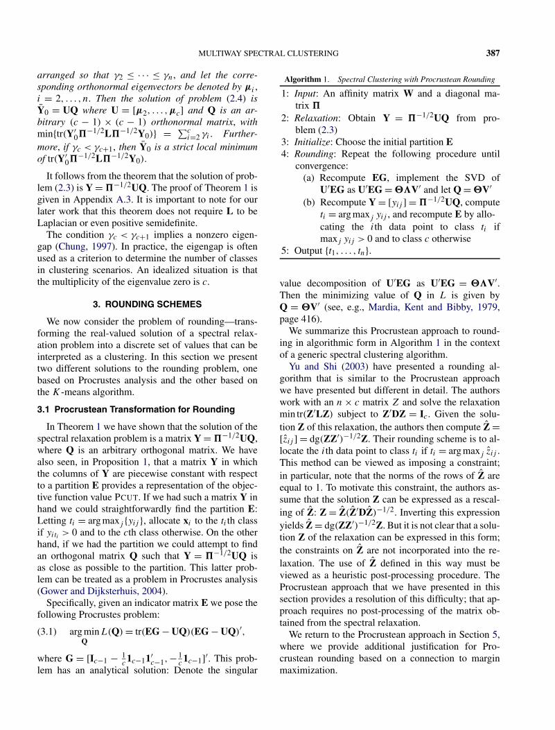
In Theorem 1 we have shown that the solution of thespectral relaxation problem is a matrix Y = �−1/2UQ,where Q is an arbitrary orthogonal matrix. We havealso seen, in Proposition 1, that a matrix Y in whichthe columns of Y are piecewise constant with respectto a partition E provides a representation of the objec-tive function value PCUT. If we had such a matrix Y inhand we could straightforwardly find the partition E:Letting ti = arg maxj {yij }, allocate xi to the ti th classif yiti > 0 and to the cth class otherwise. On the otherhand, if we had the partition we could attempt to findan orthogonal matrix Q such that Y = �−1/2UQ isas close as possible to the partition. This latter prob-lem can be treated as a problem in Procrustes analysis(Gower and Dijksterhuis, 2004).

Specifically, given an indicator matrix E we pose thefollowing Procrustes problem:

arg minQ

L(Q) = tr(EG − UQ)(EG − UQ)′,(3.1)

where G = [Ic−1 − 1c1c−11′

c−1,−1c1c−1]′. This prob-

lem has an analytical solution: Denote the singular

Algorithm 1. Spectral Clustering with Procrustean Rounding

1: Input: An affinity matrix W and a diagonal ma-trix �

2: Relaxation: Obtain Y = �−1/2UQ from pro-blem (2.3)

3: Initialize: Choose the initial partition E4: Rounding: Repeat the following procedure until

convergence:(a) Recompute EG, implement the SVD of

U′EG as U′EG = ��V′ and let Q = �V′(b) Recompute Y = [yij ] = �−1/2UQ, compute

ti = arg maxj yij , and recompute E by allo-cating the ith data point to class ti ifmaxj yij > 0 and to class c otherwise

5: Output {t1, . . . , tn}.

value decomposition of U′EG as U′EG = ��V′.Then the minimizing value of Q in L is given byQ = �V′ (see, e.g., Mardia, Kent and Bibby, 1979,page 416).

We summarize this Procrustean approach to round-ing in algorithmic form in Algorithm 1 in the contextof a generic spectral clustering algorithm.

Yu and Shi (2003) have presented a rounding al-gorithm that is similar to the Procrustean approachwe have presented but different in detail. The authorswork with an n × c matrix Z and solve the relaxationmin tr(Z′LZ) subject to Z′DZ = Ic. Given the solu-tion Z of this relaxation, the authors then compute Z =[zij ] = dg(ZZ′)−1/2Z. Their rounding scheme is to al-locate the ith data point to class ti if ti = arg maxj zij .This method can be viewed as imposing a constraint;in particular, note that the norms of the rows of Z areequal to 1. To motivate this constraint, the authors as-sume that the solution Z can be expressed as a rescal-ing of Z: Z = Z(Z′DZ)−1/2. Inverting this expressionyields Z = dg(ZZ′)−1/2Z. But it is not clear that a solu-tion Z of the relaxation can be expressed in this form;the constraints on Z are not incorporated into the re-laxation. The use of Z defined in this way must beviewed as a heuristic post-processing procedure. TheProcrustean approach that we have presented in thissection provides a resolution of this difficulty; that ap-proach requires no post-processing of the matrix ob-tained from the spectral relaxation.

We return to the Procrustean approach in Section 5,where we provide additional justification for Pro-crustean rounding based on a connection to marginmaximization.


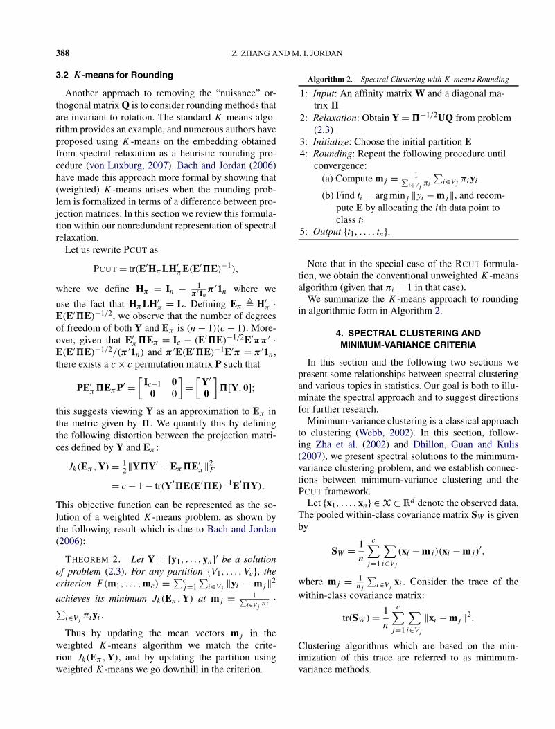
3.2 K-means for Rounding

Another approach to removing the “nuisance” or-thogonal matrix Q is to consider rounding methods thatare invariant to rotation. The standard K-means algo-rithm provides an example, and numerous authors haveproposed using K-means on the embedding obtainedfrom spectral relaxation as a heuristic rounding pro-cedure (von Luxburg, 2007). Bach and Jordan (2006)have made this approach more formal by showing that(weighted) K-means arises when the rounding prob-lem is formalized in terms of a difference between pro-jection matrices. In this section we review this formula-tion within our nonredundant representation of spectralrelaxation.

Let us rewrite PCUT as

PCUT = tr(E′HπLH′πE(E′�E)−1),

where we define Hπ = In − 1π ′1n

π ′1n where we

use the fact that HπLH′π = L. Defining Eπ � H′

π ·E(E′�E)−1/2, we observe that the number of degreesof freedom of both Y and Eπ is (n − 1)(c − 1). More-over, given that E′

π�Eπ = Ic − (E′�E)−1/2E′ππ ′ ·E(E′�E)−1/2/(π ′1n) and π ′E(E′�E)−1E′π = π ′1n,there exists a c × c permutation matrix P such that

PE′π�EπP′ =

[Ic−1 0

0 0

]=

[Y′0

]�[Y,0];

this suggests viewing Y as an approximation to Eπ inthe metric given by �. We quantify this by definingthe following distortion between the projection matri-ces defined by Y and Eπ :

Jk(Eπ ,Y) = 12‖Y�Y′ − Eπ�E′

π‖2F

= c − 1 − tr(Y′�E(E′�E)−1E′�Y).

This objective function can be represented as the so-lution of a weighted K-means problem, as shown bythe following result which is due to Bach and Jordan(2006):

THEOREM 2. Let Y = [y1, . . . ,yn]′ be a solutionof problem (2.3). For any partition {V1, . . . , Vc}, thecriterion F(m1, . . . ,mc) = ∑c

j=1∑

i∈Vj‖yi − mj‖2

achieves its minimum Jk(Eπ ,Y) at mj = 1∑i∈Vj

πi·∑

i∈Vjπiyi .

Thus by updating the mean vectors mj in theweighted K-means algorithm we match the crite-rion Jk(Eπ ,Y), and by updating the partition usingweighted K-means we go downhill in the criterion.

Algorithm 2. Spectral Clustering with K-means Rounding

1: Input: An affinity matrix W and a diagonal ma-trix �

2: Relaxation: Obtain Y = �−1/2UQ from problem(2.3)

3: Initialize: Choose the initial partition E4: Rounding: Repeat the following procedure until

convergence:(a) Compute mj = 1∑

i∈Vjπi

∑i∈Vj

πiyi

(b) Find ti = arg minj ‖yi − mj‖, and recom-pute E by allocating the ith data point toclass ti

5: Output {t1, . . . , tn}.

Note that in the special case of the RCUT formula-tion, we obtain the conventional unweighted K-meansalgorithm (given that πi = 1 in that case).

We summarize the K-means approach to roundingin algorithmic form in Algorithm 2.

4. SPECTRAL CLUSTERING ANDMINIMUM-VARIANCE CRITERIA

In this section and the following two sections wepresent some relationships between spectral clusteringand various topics in statistics. Our goal is both to illu-minate the spectral approach and to suggest directionsfor further research.

Minimum-variance clustering is a classical approachto clustering (Webb, 2002). In this section, follow-ing Zha et al. (2002) and Dhillon, Guan and Kulis(2007), we present spectral solutions to the minimum-variance clustering problem, and we establish connec-tions between minimum-variance clustering and thePCUT framework.

Let {x1, . . . ,xn} ∈ X ⊂ Rd denote the observed data.

The pooled within-class covariance matrix SW is givenby

SW = 1

n

c∑j=1

∑i∈Vj

(xi − mj )(xi − mj )′,

where mj = 1nj

∑i∈Vj

xi . Consider the trace of thewithin-class covariance matrix:

tr(SW) = 1

n

c∑j=1

∑i∈Vj

‖xi − mj‖2.

Clustering algorithms which are based on the min-imization of this trace are referred to as minimum-variance methods.


In order to establish a connection with the spectralrelaxation presented in Section 2, we define a weightedpooled within-class covariance matrix in an reproduc-ing kernel Hilbert space (RKHS) induced by a repro-ducing kernel K . In particular, assume that we aregiven the reproducing kernel K :X×X → R such thatK(xi ,xj ) = φ(xi )

′φ(xj ) for xi ,xj ∈ X, where φ(x) iscalled a feature vector corresponding to a data pointx ∈ X. In the sequel, we use the tilde notation to de-note feature vectors. Thus, the data matrix in the fea-ture space is denoted as X = [x1, x2, . . . , xn]′. The cen-tered kernel matrix takes the form K = HnXX′Hn; notethat it is positive semidefinite and satisfies K1n = 0.

Generalizing slightly, we introduce weighted ver-sions of the sample covariance matrix S, the between-class covariance matrix SB and the within-class covari-ance matrix SW :

S = 1∑ni=1 πi

n∑i=1

πi(xi − m)(xi − m)′,

SB = 1∑ni=1 πi

c∑j=1

∑i∈Vj

πi(mj − m)(mj − m)′,

SW = 1∑ni=1 πi

c∑j=1

∑i∈Vj

πi(xi − mj )(xi − mj )′,

where the πi are known positive weights, m = 1∑ni=1 πi

·∑ni=1 πi xi and mj = 1∑

i∈Vjπi

∑i∈Vj

πi xi . It is clear

that SW = S − SB .We now formulate a minimum-variance clustering

problem in the RKHS as the minimization of tr(SW),which is given by

tr(SW) = 1∑ni=1 πi

c∑j=1

∑i∈Vj

πi‖xi − mj‖2.

Like the minimization of PCUT, this minimizationis computationally infeasible in general. It is there-fore natural to consider minimizing tr(SW) by usingthe spectral relaxations presented in Section 2.2. Wepresent a way to do this in the following section.

4.1 Spectral Relaxation in the RKHS

Let us rewrite S and SB as

S = 1

π ′1n

X′Hπ�H′π X

and

SB = 1

π ′1n

X′Hπ�E(E′�E

)−1E′�H′π X,

recalling that Hπ = In − 1π ′1n

π1′n. This yields

SW = 1

π ′1n

[X′Hπ�H′

π X

− X′Hπ�E(E′�E

)−1E′�H′π X].

The minimization of tr(SW) is thus equivalent to themaximization of

T = tr(E′�H′πKHπ�E(E′�E)−1),(4.1)

because X′Hπ�H′π X is independent of E and we have

HnHπ = Hπ . Let � = [δ2ij ], where δij is the squared

distance between xi and xj , that is,

δ2ij = (xi − xj )

′(xi − xj )′

= K(xi ,xi) + K(xj ,xj ) − 2K(xi ,xj ).

Given that −12H′

π�Hπ = H′πKHπ , the minimization

of tr(SW) is thus equivalent to that of tr(E′�H′π�Hπ ·

�E(E′�E)−1).Recall that in the proof of Proposition 1, L is re-

quired to satisfy only the conditions L = L′ andL1n = 0. Note that �H′

πKHπ�1n = 0. Thus, if Y isan n × (c − 1) matrix subject to the three conditions inProposition 1, we have T = tr(Y′�H′

πKHπ�Y). Thisallows us to relax the maximization of T with respectto E as follows:

maxY∈Rn×(c−1)

tr(Y′�H′πKHπ�Y)

= tr(Y′�K�Y)(4.2)

s.t. Y′�Y = Ic−1 and Y′�1n = 0,

where the second equality in the objective is due to theidentity Y′�H′

π = Y′�. Letting Y0 = �1/2Y leads to

maxY0∈Rn×(c−1)

tr(Y′0�

1/2H′πKHπ�1/2Y0)

(4.3)s.t. Y′

0Y0 = Ic−1 and Y′0�

1/21n = 0.

This optimization problem is solved in Appendix A.4.In particular, let U be an n × (c − 1) matrix whosecolumns are the top c − 1 eigenvectors of �1/2H′

πK ·Hπ�1/2. The solution of problem (4.3) is then Y0 =UQ where Q is an arbitrary (c − 1) × (c − 1) ortho-normal matrix. Hence, the solution of problem (4.2) isY = �−1/2UQ.


4.2 Minimum Variance Formulations versus PCUT

Formulations

Since the Laplacian matrix L is symmetric and pos-itive semidefinite, its Moore–Penrose (MP) inverse isalso positive semidefinite. Thus we can regard L as theMP inverse of a kernel matrix K and investigate therelationship between the spectral relaxations obtainedfrom the minimum variance and the PCUT formula-tions. In fact, we have the following theorem, whoseproof is given in Appendix A.5.

THEOREM 3. Assume that L+ = K. If rk(L) =rk(K) = n − 1, then Y is the solution of problem (2.3)if and only if it is the solution of problem (4.2).

Thus, an equivalent formulation of spectral cluster-ing based on the PCUT criterion is obtained by con-sidering the minimum variance criterion with K = L+.Note that � consists of the diagonal elements of K+ inthe NCUT setting, so it is not expedient computation-ally to obtain � from K—we would need to calculateK+. We thus suggest defining � = In in the minimum-variance setting, corresponding to the ratio cut formu-lation.

It is also possible to start from a minimum-varianceformulation (with � = In) and obtain a RCUT prob-lem. However, in the corresponding RCUT problem,the matrix K+ is not guaranteed to be Laplacian,because the off-diagonal entries of K+ are possi-bly positive for an arbitrary kernel matrix K. Inthis case, we can let L = K+ + nβHn where β =min{maxi �=j {[K+]ij },0}. Such an L is Laplacian.Moreover, we have tr(Y′(K+ + nβHn)Y) =tr(Y′K+Y) + n(c − 1)β due to Y′Y = Ic−1 and Y′ ·1n = 0. Since min(tr(Y′(K+ + nβHn)Y)) is equiva-lent to min(tr(Y′K+Y)), it is not necessary to computethe value of β .

It is worth noting that the condition rk(L) = rk(K) =n − 1 is necessary. Without this condition, �−1/2L�−1/2 is a generalized inverse of �1/2H′

πL+Hπ

�1/2, because

�1/2H′πL+Hπ�1/2�−1/2L�−1/2�1/2H′

πL+

· Hπ�1/2 = �1/2H′πL+Hπ�1/2,

but it is not necessarily the MP inverse. In this case, it isno longer the case that �−1/2L�−1/2 and �1/2H′

πL+Hπ�1/2 are guaranteed to have the same eigenvectorsassociated with nonzero eigenvalues. Thus, in this case,even if K = L+, the solutions of (4.2) and (2.3) are dif-ferent. In summary we see that the spectral clusteringformulations based on the minimum-variance criteria

and PCUT, while closely related, are not fully equiva-lent.

Dhillon, Guan and Kulis (2007) pursue a slightly dif-ferent connection between minimum-variance criteriaand spectral relaxation. They formulate the minimum-variance criterion via the maximization of

T ′ = tr(E′�K�E(E′�E)−1),(4.4)

which is readily shown to be equal to T + π ′K ·π/(π ′1n), where T is defined by (4.1). Thus the maxi-mization of T ′ is equivalent to the maximization of T .Dhillon, Guan and Kulis (2007) then formulate the cutminimization problem as an equivalent maximizationproblem:

max(E′�(�−1 − �−1L�−1)�E(E′�E)−1)

,

and treat �−1 − �−1L�−1 as K in T ′. However,�−1 − �−1L�−1 is generally indefinite, a difficultythat the authors circumvent by letting K = ρIn − L inRCUT and K = ρD−1 + D−1WD−1 in NCUT, where ρ

is a constant chosen to make K positive semidefinite.The idea of considering a kernel matrix that is the

MP inverse of a Laplacian matrix will return in latersections, in particular in Section 5.1 where we will seethat it allows us to provide a geometrical interpreta-tion for spectral clustering, and in Section 6, where wepresent a probabilistic interpretation of spectral relax-ation.

5. SPECTRAL CLUSTERING: A MARGIN-BASEDPERSPECTIVE

In this section we consider a margin-based per-spective on spectral clustering. First, we show thatthe margin-based perspective provides us with insightinto the relationship between spectral embedding androunding. In particular, we show that the problems in(2.3) and (4.2) can be understood in terms of the fit-ting of hyperplanes in an RKHS. For a data point x, weshow that the elements of the embedding y are propor-tional to the signed distances of feature vector x to eachof these hyperplanes. This provides support for the Pro-crustean rounding in which rounding is achieved bynonmaximum suppression of the elements of y. Sec-ond, we provide some additional direct justification forthe Procrustean approach, showing that the roundingproblem can be analyzed in terms of the approximationof a margin-based multiway classification criterion.


5.1 Hyperplanes in the RKHS

Let us consider a multiway classification problem.That is, we consider a problem in which data points arepairs, (xi , ti), where ti is the label of the ith data point.Using the same notation as in Section 4, the multiwayclassification problem has the following standard for-mulation in an RKHS based on a kernel function K :

minβ0,B

tr(B′KB) + γ

n

n∑i=1

fti (B′ki + β0),(5.1)

where fj (·) is a convex surrogate of the 0–1 loss, ki =(K(x1,xi), . . . ,K(xn,xi ))

′ is the ith column of thekernel matrix K, B = [b1, . . . ,bc−1] is an n × (c − 1)

matrix of regression vectors, β0 is a (c − 1) × 1 vectorof intercepts and γ > 0 is a regularization parameter.We can use this optimization problem as the basis ofa clustering formulation by simply omitting the termγn

∑ni=1 fti (·), reflecting the fact that we have no la-

beled data in the clustering setting. We obtain

minB

tr(B′KB)

(5.2)s.t. B′K�1n = 0 and B′K�KB = Ic−1.

We now consider problem (5.2) from two points ofview. From the first point of view, we let Y = KB andtransform (5.2) into

minY

tr(Y′K+Y)

(5.3)s.t. Y′�1n = 0 and Y′�Y = Ic−1,

where we have used the identity K = KK+K. It isreadily seen that (5.3), and hence (5.2), is identical withthe spectral relaxation in (2.3) by taking K+ = L. Wealso obtain a relationship between (5.3) and (4.2) fromSection 4.2; in particular, in the special case in whichrk(K) = n − 1, it follows from Theorem 3 that (5.3)and (4.2) are equivalent.

From a second point of view, we let S = X′B (re-call that X is the data matrix in the feature space). Theproblem (5.2) is then transformed into

minS

tr(S′S)

(5.4)s.t. S′X′�1n = 0 and S′X′�XS = Ic−1.

Letting S = [s1, . . . , sc−1] denote the solution of (5.4),the equations s′

j x = 0, j = 1, . . . , c − 1, define hy-perplanes that pass through the weighted centroid∑n

i=1 πi xi of the feature vectors xi . Moreover, thesigned distance between feature vector xi and the hy-perplane s′

j x = 0 is s′j xi . Recall that Y = [yij ] = KB =

XX′B = XS. We thus have yij = s′j xi . That is, yij

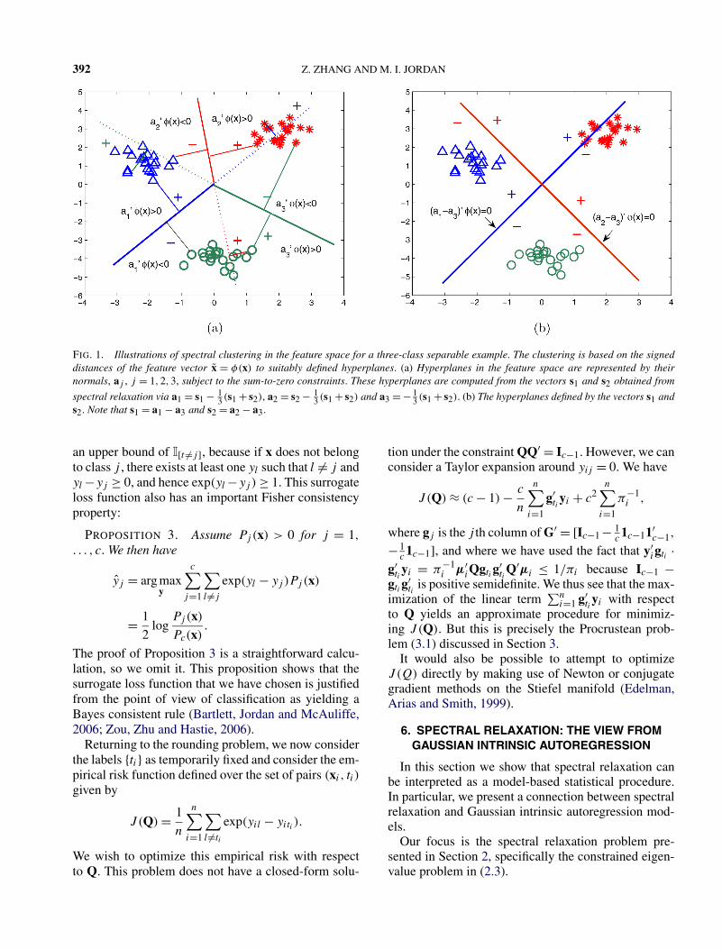
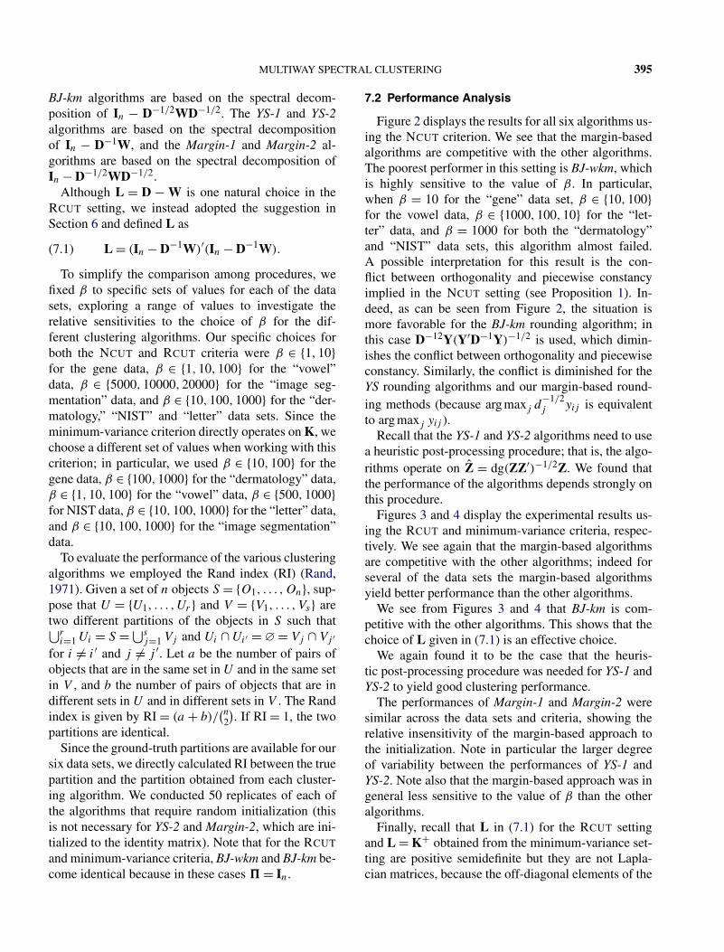
is the signed distance of xi to the j th hyperplane.We can therefore interpret the spectral relaxation in(2.3) and (4.2) as yielding vectors whose elementsare—using the language of multiway classification—margin vectors. Given this interpretation, it is reason-able to allocate labels by finding the maximum elementof (yi1, . . . , yi,c−1,0). This motivates the Procrusteanapproach to rounding, which can be viewed as identify-ing boundaries between clusters by projecting featurevectors onto hyperplanes in an RKHS. A graphical in-terpretation of this result is provided in Figure 1.

5.2 Margin-Based Rounding Scheme

We can also provide a direct connection betweenclassification and rounding. Let us return to the objec-tive function in (5.1), which we rewrite as

minY

tr(Y′K+Y) + γ

n

n∑i=1

fti (yi )

by letting Y = KB and setting β0 = 0. Assume thatwe have obtained a matrix Y from spectral relaxationand recall that Y depends on an arbitrary orthogonalmatrix Q. From the classification perspective we canview the subsequent rounding problem as the problemof minimizing the classification loss 1

n

∑ni=1 fti (yi ) un-

der the constraint QQ′ = Ic−1. In this section we ex-plore some of the consequences of this perspective.

In the multiway classification problem, we defineclass-conditional probabilities Pj (x) for the c classesj = 1, . . . , c. Using this notation, we define the ex-pected error at x as follows:

R(x,y) =c∑

j=1

I[t �=j ]Pj (x),(5.5)

where t = arg maxj yj or t = c if max{yj } < 0 andwhere I[#] defines the 0–1 loss: it is 1 if # is true and0 otherwise. Since I[·] is a non-convex objective func-tion that leads to an intractable optimization problem,the standard practice in the classification literature is toreplace I[·] with a “surrogate loss function” fj (y) thatis an upper bound on the 0–1 loss (Bartlett, Jordan andMcAuliffe, 2006; Shen and Wang, 2007).

The surrogate loss function that we consider in thecurrent paper is the following exponential loss:

fj (y) = ∑l �=j

exp(yl − yj ),(5.6)

where for convenience we extend y to a c-dimensionalvector in which yc = 0. Note that the variables to be op-timized are the entries of the matrix Q. Clearly, fj (y) is


FIG. 1. Illustrations of spectral clustering in the feature space for a three-class separable example. The clustering is based on the signeddistances of the feature vector x = φ(x) to suitably defined hyperplanes. (a) Hyperplanes in the feature space are represented by theirnormals, aj , j = 1,2,3, subject to the sum-to-zero constraints. These hyperplanes are computed from the vectors s1 and s2 obtained from

spectral relaxation via a1 = s1 − 13 (s1 + s2), a2 = s2 − 1

3 (s1 + s2) and a3 = − 13 (s1 + s2). (b) The hyperplanes defined by the vectors s1 and

s2. Note that s1 = a1 − a3 and s2 = a2 − a3.

an upper bound of I[t �=j ], because if x does not belongto class j , there exists at least one yl such that l �= j andyl −yj ≥ 0, and hence exp(yl −yj ) ≥ 1. This surrogateloss function also has an important Fisher consistencyproperty:

PROPOSITION 3. Assume Pj (x) > 0 for j = 1,

. . . , c. We then have

yj = arg maxy

c∑j=1

∑l �=j

exp(yl − yj )Pj (x)

= 1

2log

Pj (x)

Pc(x).

The proof of Proposition 3 is a straightforward calcu-lation, so we omit it. This proposition shows that thesurrogate loss function that we have chosen is justifiedfrom the point of view of classification as yielding aBayes consistent rule (Bartlett, Jordan and McAuliffe,2006; Zou, Zhu and Hastie, 2006).

Returning to the rounding problem, we now considerthe labels {ti} as temporarily fixed and consider the em-pirical risk function defined over the set of pairs (xi , ti)

given by

J (Q) = 1

n

n∑i=1

∑l �=ti

exp(yil − yiti ).

We wish to optimize this empirical risk with respectto Q. This problem does not have a closed-form solu-

tion under the constraint QQ′ = Ic−1. However, we canconsider a Taylor expansion around yij = 0. We have

J (Q) ≈ (c − 1) − c

n

n∑i=1

g′ti

yi + c2n∑

i=1

π−1i ,

where gj is the j th column of G′ = [Ic−1 − 1c1c−11′

c−1,

−1c1c−1], and where we have used the fact that y′

igti ·g′ti

yi = π−1i μ′

iQgti g′ti

Q′μi ≤ 1/πi because Ic−1 −gti g

′ti

is positive semidefinite. We thus see that the max-imization of the linear term

∑ni=1 g′

tiyi with respect

to Q yields an approximate procedure for minimiz-ing J (Q). But this is precisely the Procrustean prob-lem (3.1) discussed in Section 3.

It would also be possible to attempt to optimizeJ (Q) directly by making use of Newton or conjugategradient methods on the Stiefel manifold (Edelman,Arias and Smith, 1999).

6. SPECTRAL RELAXATION: THE VIEW FROMGAUSSIAN INTRINSIC AUTOREGRESSION

In this section we show that spectral relaxation canbe interpreted as a model-based statistical procedure.In particular, we present a connection between spectralrelaxation and Gaussian intrinsic autoregression mod-els.

Our focus is the spectral relaxation problem pre-sented in Section 2, specifically the constrained eigen-value problem in (2.3).


Recall that the Laplacian matrix L is a positive semi-definite matrix; moreover, the pseudoinverse L+ ispositive semidefinite and can be viewed as a kernel ma-trix. We found this perspective useful in our discussionof minimum-variance clustering in Section 4.2; notealso that (Saerens et al., 2004) have explored connec-tions between spectral embedding and random walkson graphs using the fact that the elements of L+ areclosely related to the commute-time distances obtainedfrom a random walk on the graph. In this section, wetake the interpretation of L+ in a different direction,using it to make the connection to Gaussian intrinsicautoregressions.

Denote K = L+ where L = D−W. Let us model then×(c−1) matrix Y as a singular matrix-variate normaldistribution Nn,c−1(0, σ 2K ⊗ Ic−1) where we followthe notation for matrix-variate normal distributions in(Gupta and Nagar, 2000). That is,

p(Y) ∝ exp(− 1

2σ 2 tr(Y′LY)

).

Let us set σ 2 = 1/ tr (�K) so that E(Y′�Y) = σ 2

tr(�K)Ic−1 = Ic−1. Finally, we impose the constraintY′�1n = 0 in order to remove the redundancy K+1n =0 in K+. We thus obtain the following proposition.

PROPOSITION 4. The relaxation problem in (2.3)is equivalent to the maximization of the log likeli-hood p(Y) under the constraints Y′�Y = Ic−1 andY′�1n = 0.

We obtain a statistical interpretation of spectral re-laxation from the fact that a multivariate normal dis-tribution can be equivalently expressed as a Gaussianconditional autoregression (CAR) (Besag 1974; Mar-dia 1988). Indeed, given Y ∼ Nn,c−1(0, σ 2K ⊗ Ic−1),we have that the yi can be characterized as (c − 1)-dimensional CARs with

E(yi |yj , j �= i) = −∑j �=i

lij

liiyj =

n∑j=1

wij

liiyj ,

(6.1)

Var(yi |yj , j �= i) = σ 2

liiIc−1.

That is, we have yi |{yj : j �= i} ∼ Nc−1(∑n

j=1wij

liiyj ,

σ 2

liiIc−1), for i = 1, . . . , n. Since K is positive semidef-

inite but not positive definite, Besag and Kooperberg(1995) referred to such conditional autoregressions asGaussian intrinsic autoregressions.

The CAR model implicitly requires wii = 0 andlii = ∑n

j=1 wij . In spectral embedding and cluster-ing (Guattery and Miller, 2000; Belkin and Niyogi,

2002; Ng, Jordan and Weiss, 2002), the wij are usu-ally used to assert adjacency or similarity relationshipsbetween the yi . We will see shortly that these adja-cency or similarity relationships have an interpretationas conditional independencies.

Since D − W is positive semidefinite, D − ωW ispositive definite for ω ∈ (0,1). This fact has been usedto devise CAR models based on D − ωW such thatE(yi |yj , j �= i) = ω

∑nj=1

wij

liiyj (see, e.g., Carlin and

Banerjee, 2003). We now have

E(yiy′j |yl , l �= i, j) = ωlij

ω2l2ij − lii ljj

σ 2Ic−1.

As a result, lij = 0 (or wij = 0) implies that yi ⊥⊥yj |{yl : l �= i, j}; that is, yi is conditionally indepen-dent of yj given the remaining vectors. This Markovproperty also holds for Gaussian intrinsic autoregres-sions (Besag and Kooperberg, 1995).

This perspective sheds light on some of the rela-tionships between the NCUT and RCUT formulationsof spectral relaxation. Recall that since � = D in theNCUT setting, we impose the constraints Y′DY = Ic−1and Y′D1n = 0. On the other hand, the RCUT formu-lation uses the constraints Y′Y = Ic−1 and Y′1n = 0because � = In. Theorem 1 shows that the solu-tion of the NCUT is based on �−1/2L�−1/2 = In −D−1/2WD−1/2, which is a so-called normalized graphLaplacian. The solution of the RCUT problem is basedon the unnormalized graph Laplacian L. Now Propo-sition 1 reveals a problematic aspect of the NCUT

formulation—piecewise constancy of the columns of Yis accompanied by a lack of orthogonality of thesecolumns. Two natural desiderata of spectral cluster-ing are in conflict in the NCUT formulation. This con-flict between orthogonality and piecewise constancy isnot present for RCUT. However, the existing empiri-cal results showed that the normalized graph Laplaciantends to outperform the unnormalized graph Laplacian.Moreover, von Luxburg, Belkin and Bousquet (2008)provided theoretical evidence of the superiority of thenormalized graph Laplacian.

This seeming paradox can be resolved by using analternative choice for L in the RCUT formulation. Letus set L = (In − C)′(In − C), where C = [cij ] is ann × n nonnegative matrix such that cii = 0 for all i

and C1n = 1n. Such a L is positive semidefinite but nolonger Laplacian. Since L1n = 0, we can still solve thespectral relaxation problem (2.4) using Theorem 1.

Our experimental results in Section 7 show thatthis novel RCUT formulation is very effective. It is


also worth noting that we can connect this formula-tion to the simultaneous autoregression (SAR) modelof Besag (1974). In particular, the yi are now specifiedby n simultaneous equations:

yi =n∑

j=1

cij yj + εi , i = 1, . . . , n,

where the εi are independent normal vectors fromNc−1(0, σ 2Ic−1). This equation can be written in ma-trix form as follows:

Y = CY + �

with � = [ε1, . . . ,εn]′ ∼ Nn,c−1(0, σ 2In ⊗ Ic−1

).

We thus have Y ∼ Nn,c−1(0, σ 2K ⊗ Ic−1

)with K+ =

(In − C)′(In − C). In practice, we are especiallyconcerned with the case in which C = D−1W. It isworth noting that In − D−1/2WD−1/2 and In − D−1Whave the same eigenvalues, while the squared sin-gular values of In − D−1W are the eigenvalues of(In − D−1W)′(In − D−1W). We thus obtain an inter-esting new relationship between the NCUT formulationand the RCUT formulation.

7. EXPERIMENTS

Although our principal focus has been to provide aunifying perspective on spectral clustering, our analy-sis has also provided novel spectral algorithms, and itis of interest to compare the performance of these algo-rithms to existing algorithms. In this section we reportthe results of experiments conducted with six publiclyavailable data sets: five data sets from the UCI machinelearning repository (the dermatology data, the voweldata, the NIST optical handwritten digit data, the let-ter data and the image segmentation data) as well asa set of gene expression data analyzed by Yeung et al.(2001).

In the dermatology data, there are 366 patients, 8 ofwhom are excluded due to missing information, with34 features. The data are clustered into six classes. Westandardized the data to have zero mean and unit vari-ance. The NIST data set contains the handwritten digits0–9, where each instance consists of a 16 × 16 pixeland where digits are treated as classes. We selected1000 digits, with 100 instances per digit, for our ex-periments. The vowel data set contains the elevensteady-state vowels of British English. The letter dataset consists of images of the letters “A” to “Z.” Inour experiments we selected the first 10 letters with195, 199, 182, 207, 203, 210, 226, 196, 188 and 172

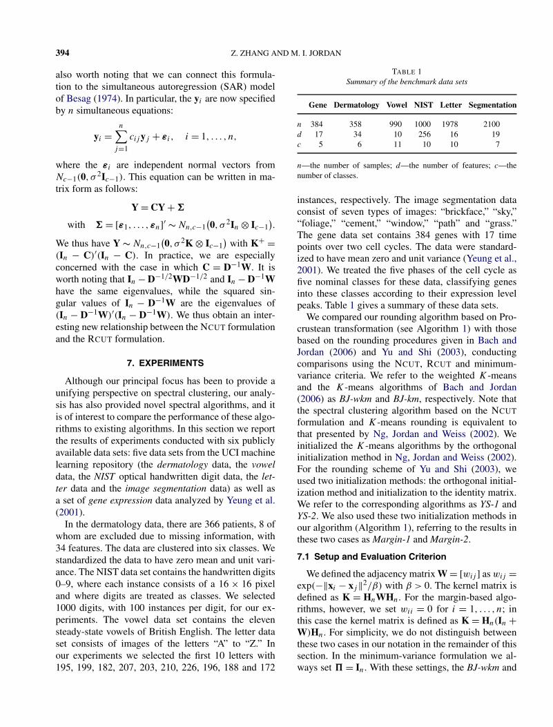
TABLE 1Summary of the benchmark data sets

Gene Dermatology Vowel NIST Letter Segmentation

n 384 358 990 1000 1978 2100d 17 34 10 256 16 19c 5 6 11 10 10 7

n—the number of samples; d—the number of features; c—thenumber of classes.

instances, respectively. The image segmentation dataconsist of seven types of images: “brickface,” “sky,”“foliage,” “cement,” “window,” “path” and “grass.”The gene data set contains 384 genes with 17 timepoints over two cell cycles. The data were standard-ized to have mean zero and unit variance (Yeung et al.,2001). We treated the five phases of the cell cycle asfive nominal classes for these data, classifying genesinto these classes according to their expression levelpeaks. Table 1 gives a summary of these data sets.

We compared our rounding algorithm based on Pro-crustean transformation (see Algorithm 1) with thosebased on the rounding procedures given in Bach andJordan (2006) and Yu and Shi (2003), conductingcomparisons using the NCUT, RCUT and minimum-variance criteria. We refer to the weighted K-meansand the K-means algorithms of Bach and Jordan(2006) as BJ-wkm and BJ-km, respectively. Note thatthe spectral clustering algorithm based on the NCUT

formulation and K-means rounding is equivalent tothat presented by Ng, Jordan and Weiss (2002). Weinitialized the K-means algorithms by the orthogonalinitialization method in Ng, Jordan and Weiss (2002).For the rounding scheme of Yu and Shi (2003), weused two initialization methods: the orthogonal initial-ization method and initialization to the identity matrix.We refer to the corresponding algorithms as YS-1 andYS-2. We also used these two initialization methods inour algorithm (Algorithm 1), referring to the results inthese two cases as Margin-1 and Margin-2.

7.1 Setup and Evaluation Criterion

We defined the adjacency matrix W = [wij ] as wij =exp(−‖xi − xj‖2/β) with β > 0. The kernel matrix isdefined as K = HnWHn. For the margin-based algo-rithms, however, we set wii = 0 for i = 1, . . . , n; inthis case the kernel matrix is defined as K = Hn(In +W)Hn. For simplicity, we do not distinguish betweenthese two cases in our notation in the remainder of thissection. In the minimum-variance formulation we al-ways set � = In. With these settings, the BJ-wkm and


BJ-km algorithms are based on the spectral decom-position of In − D−1/2WD−1/2. The YS-1 and YS-2algorithms are based on the spectral decompositionof In − D−1W, and the Margin-1 and Margin-2 al-gorithms are based on the spectral decomposition ofIn − D−1/2WD−1/2.

Although L = D − W is one natural choice in theRCUT setting, we instead adopted the suggestion inSection 6 and defined L as

L = (In − D−1W)′(In − D−1W).(7.1)

To simplify the comparison among procedures, wefixed β to specific sets of values for each of the datasets, exploring a range of values to investigate therelative sensitivities to the choice of β for the dif-ferent clustering algorithms. Our specific choices forboth the NCUT and RCUT criteria were β ∈ {1,10}for the gene data, β ∈ {1,10,100} for the “vowel”data, β ∈ {5000,10000,20000} for the “image seg-mentation” data, and β ∈ {10,100,1000} for the “der-matology,” “NIST” and “letter” data sets. Since theminimum-variance criterion directly operates on K, wechoose a different set of values when working with thiscriterion; in particular, we used β ∈ {10,100} for thegene data, β ∈ {100,1000} for the “dermatology” data,β ∈ {1,10,100} for the “vowel” data, β ∈ {500,1000}for NIST data, β ∈ {10,100,1000} for the “letter” data,and β ∈ {10,100,1000} for the “image segmentation”data.

To evaluate the performance of the various clusteringalgorithms we employed the Rand index (RI) (Rand,1971). Given a set of n objects S = {O1, . . . ,On}, sup-pose that U = {U1, . . . ,Ur} and V = {V1, . . . , Vs} aretwo different partitions of the objects in S such that⋃r

i=1 Ui = S = ⋃sj=1 Vj and Ui ∩ Ui′ = ∅ = Vj ∩ Vj ′

for i �= i′ and j �= j ′. Let a be the number of pairs ofobjects that are in the same set in U and in the same setin V , and b the number of pairs of objects that are indifferent sets in U and in different sets in V . The Randindex is given by RI = (a + b)/

(n2

). If RI = 1, the two

partitions are identical.Since the ground-truth partitions are available for our

six data sets, we directly calculated RI between the truepartition and the partition obtained from each cluster-ing algorithm. We conducted 50 replicates of each ofthe algorithms that require random initialization (thisis not necessary for YS-2 and Margin-2, which are ini-tialized to the identity matrix). Note that for the RCUT

and minimum-variance criteria, BJ-wkm and BJ-km be-come identical because in these cases � = In.

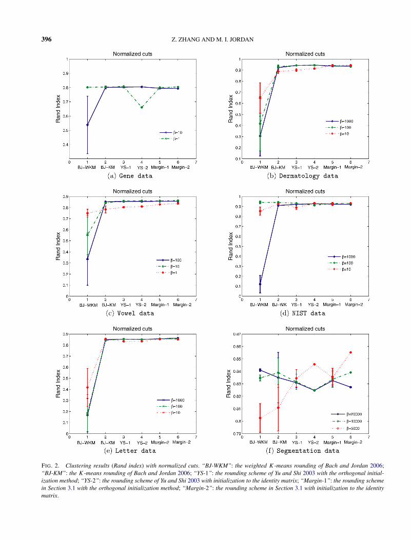
7.2 Performance Analysis

Figure 2 displays the results for all six algorithms us-ing the NCUT criterion. We see that the margin-basedalgorithms are competitive with the other algorithms.The poorest performer in this setting is BJ-wkm, whichis highly sensitive to the value of β . In particular,when β = 10 for the “gene” data set, β ∈ {10,100}for the vowel data, β ∈ {1000,100,10} for the “let-ter” data, and β = 1000 for both the “dermatology”and “NIST” data sets, this algorithm almost failed.A possible interpretation for this result is the con-flict between orthogonality and piecewise constancyimplied in the NCUT setting (see Proposition 1). In-deed, as can be seen from Figure 2, the situation ismore favorable for the BJ-km rounding algorithm; inthis case D−12Y(Y′D−1Y)−1/2 is used, which dimin-ishes the conflict between orthogonality and piecewiseconstancy. Similarly, the conflict is diminished for theYS rounding algorithms and our margin-based round-ing methods (because arg maxj d

−1/2j yij is equivalent

to arg maxj yij ).Recall that the YS-1 and YS-2 algorithms need to use

a heuristic post-processing procedure; that is, the algo-rithms operate on Z = dg(ZZ′)−1/2Z. We found thatthe performance of the algorithms depends strongly onthis procedure.

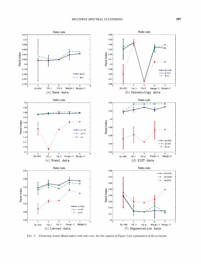
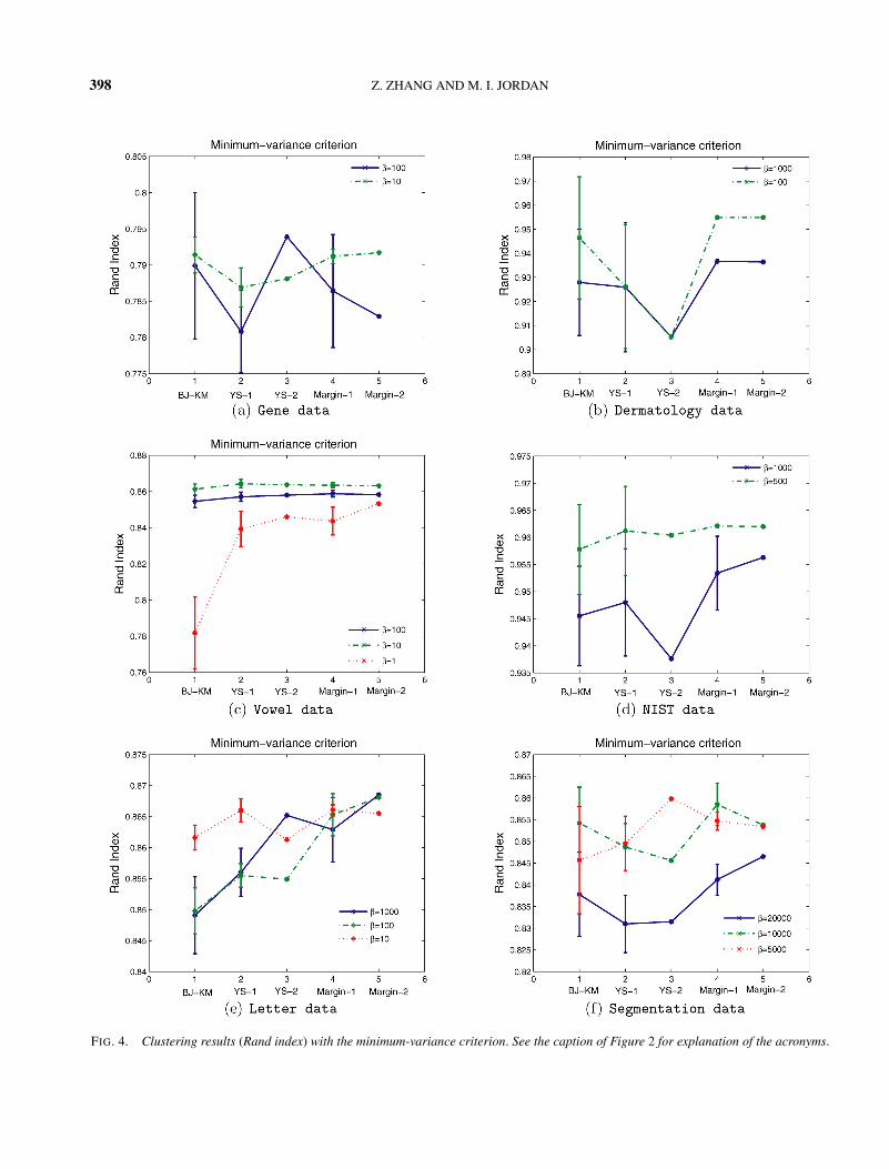
Figures 3 and 4 display the experimental results us-ing the RCUT and minimum-variance criteria, respec-tively. We see again that the margin-based algorithmsare competitive with the other algorithms; indeed forseveral of the data sets the margin-based algorithmsyield better performance than the other algorithms.

We see from Figures 3 and 4 that BJ-km is com-petitive with the other algorithms. This shows that thechoice of L given in (7.1) is an effective choice.

We again found it to be the case that the heuris-tic post-processing procedure was needed for YS-1 andYS-2 to yield good clustering performance.

The performances of Margin-1 and Margin-2 weresimilar across the data sets and criteria, showing therelative insensitivity of the margin-based approach tothe initialization. Note in particular the larger degreeof variability between the performances of YS-1 andYS-2. Note also that the margin-based approach was ingeneral less sensitive to the value of β than the otheralgorithms.

Finally, recall that L in (7.1) for the RCUT settingand L = K+ obtained from the minimum-variance set-ting are positive semidefinite but they are not Lapla-cian matrices, because the off-diagonal elements of the


FIG. 2. Clustering results (Rand index) with normalized cuts. “BJ-WKM”: the weighted K-means rounding of Bach and Jordan 2006;“BJ-KM”: the K-means rounding of Bach and Jordan 2006; “YS-1”: the rounding scheme of Yu and Shi 2003 with the orthogonal initial-ization method; “YS-2”: the rounding scheme of Yu and Shi 2003 with initialization to the identity matrix; “Margin-1”: the rounding schemein Section 3.1 with the orthogonal initialization method; “Margin-2”: the rounding scheme in Section 3.1 with initialization to the identitymatrix.


FIG. 3. Clustering results (Rand index) with ratio cuts. See the caption of Figure 2 for explanation of the acronyms.


FIG. 4. Clustering results (Rand index) with the minimum-variance criterion. See the caption of Figure 2 for explanation of the acronyms.


W = L−D are possibly negative. Nonetheless, our ex-perimental results showed that these two choices arestill effective. Thus cuts can be defined through non-Laplacian matrices. Although such cuts lose their orig-inal interpretation in terms of the graph partition, aswe have shown they do have a clear statistical inter-pretation in terms of Gaussian intrinsic autoregressionmodels.

8. DISCUSSION

In this paper we have presented a margin-basedperspective on multiway spectral clustering. We haveshown that both aspects of spectral clustering—relaxa-tion and rounding—can be given an interpretation interms of margins. The major advantage of this perspec-tive is that it ties spectral clustering to the large litera-ture on margin-based classification. The margin-basedperspective has several additional consequences: (1) itpermits a deeper understanding of the relationship be-tween the normalized cut and ratio cut formulations ofspectral clustering; (2) it strengthens the connectionsbetween the minimum-variance criterion and spectralclustering; and (3) it yields a statistical interpretationof spectral clustering in terms of Gaussian intrinsic au-toregressions. Also, the preliminary empirical evidencethat we presented suggests that the algorithms moti-vated by the margin-based perspective are competitivewith existing spectral clustering algorithms.

One of the most useful consequences of the margin-based perspective is the interpretation that it yields ofspectral clustering in terms of projection onto hyper-planes in a reproducing kernel Hilbert space (see Fig-ure 1). This interpretation shows that the performanceof the margin-based clustering algorithms depends onthe separability of the feature vectors. This suggeststhat the algorithmic problem of choosing the similar-ity matrix W or kernel matrix K so as to increaseseparability is an important topic for further research;see Bach and Jordan (2006) and Meila and Shi (2000)for initial work along these lines.

Although we have focused on undirected graphs inour treatment, it is also worth noting the possibilityof considering clustering in a directed graph with theasymmetric weighted matrix D−1W (Meila and Pent-ney, 2007). This can be related to our discussion inSection 6, where we suggested the use of the matrixL = (In − D−1W)′(In − D−1W) in the RCUT setting.The experimental results in Section 7 showed that sucha suggestion is promising. Moreover, although L is nolonger Laplacian, the corresponding spectral relaxation

can be interpreted as a simultaneous autoregressionmodel. The relationship between simultaneous autore-gression and conditional autoregression (Ripley, 1981)may provide connections between spectral clusteringin undirected graphs and directed graphs. We intend toexplore this issue in future work.

In delineating a relationship between the PCUT cri-terion and the kernel minimum-variance criterion, wehave proven that the relaxation problems (2.3) and(4.2) have the same solution whenever rk(L) = n − 1and L+ = K. This leads to the question as to whetherthe original unrelaxed problems—that is, the mini-mization of PCUT and the maximization of T with re-spect to discrete partition matrix E— have the same so-lution under the conditions rk(L) = n−1 and L+ = K.This is currently an open problem.

APPENDIX

A.1 Proof of Proposition 1

Since the columns of Y are piecewise constantwith respect to the partition E, we can express Y asY = E� for some � ∈ R

c×(c−1). Let Y0 = �1/2Y,�0 = [�, α1c], a c×c matrix, and Z = [Y0, α�1/21n],where α = 1/

√1′n�1n. We have �−1/2Z = E�0

and Z′Z = [Y0, α�1/21n]′[Y0, α�1/21n] = Ic due toE1c = 1n, Y′

0Y0 = Y′�Y = Ic−1 and Y′0�

1/21n =Y′�1n = 0. Furthermore, we have � ′

0E′�E�0 =Z′Z = Ic. Since �0 and E′�E are square, �0 andE′�E are invertible. Hence �0�

′0 = (E′�E)−1. We

now have

tr(Y′LY) = tr(Y′0�

−1/2L�−1/2Y0)

= tr(Z′�−1/2L�−1/2Z) = tr(� ′0E′LE�0)

= tr(E′LE�0�′0) = tr(E′LE(E′�E)−1),

completing the proof.

A.2 The Proof of Proposition 2

In this section we provide a constructive proof ofProposition 2 by establishing the existence of � . Wealso provide an example of the construction in the spe-cial case of c = 4 and � = In.

Let (E′�E)−1 = diag(1/β1, . . . ,1/βc) and β =(β1, . . . , βc)

′. We then have 1′n�1n = π ′1n = β ′1c and

E′�1n = β . In the proof in Appendix A.1, we obtain�0�

′0 = (E′�E)−1. Thus,

�� ′ = diag(1/β1, . . . ,1/βc) − 1

π ′1n

1c1′c

(denoted A).


In order to make the above equation hold, it is nec-essary for A to be positive semidefinite. Given anynonzero b = (b1, . . . , bc)

′ ∈ Rc, we have

b′ diag(β)A diag(β)b/(π ′1n)

=c∑

j=1

βj

π ′1n

b2j −

(∑j=1

βj

π ′1n

bj

)2

≥ 0,

since the function f (x) = x2 is convex. This impliesthat A positive semidefinite. Furthermore, it is easy toobtain Aβ = 0. Using the SVD of A, we are alwaysable to obtain a � such that �� ′ = A and � ′β = 0.Consequently, we have

1′n�E� = β ′� = 0 and � ′E′�E� = Ic−1.

The latter equality comes from

Ic = � ′0E′�E�0 =

[� ′α1′

c

]E′�E[�, α1c]

=[� ′E′�E� 0

0 1

].

EXAMPLE 1. Let η = π ′1n and ηj = ∑i∈Vj

πi .Assume that � = (ψ1, . . . ,ψc−1)

′ where ψ ′1 =

(√

η−η1√ηη1

,−√

η1√η(η−η1)

1′c−1) and

ψ ′l =

(0 ∗ 1′

l−1,

√∑cj=l+1 ηj√

ηl

∑cj=l ηj

,

√ηl√∑c

j=l ηj

∑cj=l+1 ηj

1c−l

)

for l = 2, . . . , c − 1. For instance, if c = 4, we have

� =

⎡⎢⎢⎢⎢⎢⎢⎢⎣

√η−η1√ηη1

0 0

−√

η1√η(η−η1)

√η3+η4√

η2(η−η1)0

−√

η1√η(η−η1)

−√

η2√(η3+η4)(η−η1)

√η4√

(η3+η4)η3

−√

η1√η(η−η1)

−√

η2√(η3+η4)(η−η1)

−√

η3√(η3+η4)η4

⎤⎥⎥⎥⎥⎥⎥⎥⎦.

It is easily verified that Y = E� satisfies the condi-tions (a)–(c) listed in Proposition 1. Let a1, . . . ,ac de-note the row vectors of � . We note that an arbitrarycollection of c − 1 vectors from the set a1, . . . ,ac arelinearly independent. The convex hull of a1, . . . ,ac isthus a (c − 1)-dimensional simplex. (A d-dimensionalsimplex is the convex hull of an affinely independentpoint set in R

d . A regular d-dimensional simplex isthe convex hull of d + 1 points with all pairs of points

having equal distances.) In addition, we have that thesquared distance between ai and aj is

‖ai − aj‖2 = 1

ηi

+ 1

ηj

for i �= j.

Note that we have η = n and ηj = nj when � = In.In particular, if � = In and n1 = · · · = nc = n

c, the ai

constitute the vertices of a (c − 1)-dimensional regularsimplex.

A.3 The Proof of Theorem 1

This theorem is a variation on a standard result inlinear algebra; for completeness we present a proof.Let S = �−1/2L�−1/2 and consider the following La-grangian:

L(Y0,A,b)

= tr(Y′

0SY0) − tr(A(Y′

0Y0 − Ic−1)) − b′Y′0�

1/21n,

where A is a (c − 1) × (c − 1) symmetric matrix ofLagrange multipliers and b is a (c − 1) × 1 vector ofLagrange multipliers. We differentiate to obtain

∂L

∂Y0= 2SY0 − 2Y0A − �1/21nb′.

Letting ∂L∂Y0

= 0 leads to

2SY0 − 2Y0A − �1/21nb′ = 0,

from which we have

21′n�

1/2SY0 − 21′n�

1/2Y0A − 1′n�1nb′ = 0.

This implies b = 0. Accordingly, we obtain

SY0 = Y0A.

We now take the eigendecomposition of A, lettingA = Q′ 1Q where Q is a (c − 1) × (c − 1) ortho-normal matrix and 1 is a (c − 1) × (c − 1) diago-nal matrix. We note that the diagonal entries of 1and the columns of Y0Q′ are the eigenvalues and theassociated eigenvectors of S. Clearly, �1/21n is theeigenvector of S associated with eigenvalue 0. Wenow let 1 = diag(γ2, . . . , γc). We thus have Y0 =[μ2, . . . ,μc]Q. Obviously, Y0 satisfies Y′

0Y0 = Ic−1

and Y′0�

1/21n = 0 due to μ′i�

1/21n = 0 for i �= 1.To verify that Y0 is the solution of problem (2.4), we

consider the Hessian matrix of L with respect to Y0.Let vec(Y′

0) = (y11, . . . , y1,c−1, y21, . . . , yn,c−1)′. The

Hessian matrix is then given by

H(Y0) = ∂2L

∂ vec(Y′0) ∂ vec(Y′

0)′ = Ic−1 ⊗ S − A ⊗ In.


Let B be an arbitrary nonzero n × (c − 1) matrixsuch that B′[μ1, . . . ,μc] = 0. We can always expressB = [μc+1, . . . ,μn]� where � = [φ1, . . . ,φc−1] is an(n−c)×(c−1) matrix. Denoting 2 = diag(γc+1, . . . ,

γn), we have

vec((BQ)′)′H(Y0)vec((BQ)′)= tr(Q′B′SBQ) − tr(AQ′B′BQ)

= tr(B′SB) − tr( 1B′B) = tr(�′ 2�) − tr( 1�′�)

=c−1∑i=1

φ′i 2φi −

c−1∑i=1

γi+1φ′iφi

=c−1∑i=1

φ′i ( 2 − γi+1In−c)φi ≥ 0.

If γc > γc+1, then the matrices 2 − γi+1In−c, i =1, . . . , c − 1, are positive definite. Thus, the above in-equality is strict. This shows that Y0 is a strict localminimum of tr(Y′

0�−1/2L�−1/2Y0) under the condi-

tions Y′0Y0 = Ic−1 and Y′

0�1/21n = 0.

A.4 The Solution of Problem (4.3)

Let T = �1/2H′πKHπ�1/2 and consider the follow-

ing Lagrangian:

L(Y0,A,b)

= tr(Y′0TY0) − tr

(A(Y′

0Y0 − Ic−1)) − b′Y′

0�1/21n,

where A is a (c − 1) × (c − 1) symmetric matrix ofLagrange multipliers and b is a (c − 1) × 1 vector ofLagrange multipliers. Differentiating, we obtain

∂L

∂Y0= 2TY0 − 2Y0A − �1/21nb′.

Letting ∂L∂Y0

= 0 leads to

2TY0 − 2Y0A − �1/21nb′ = 0,

from which we have

21′n�

1/2TY0 − 21′n�

1/2Y0A − 1′n�1nb′ = 0.

Since 1′n�

1/2T = 1′n�H′

πKHπ�1/2 = 1′nHπ�K ·

Hπ�1/2 = 0, we obtain b = 0. This implies

TY0 = Y0A.

Now following the proof in Appendix A.3, we find thatthe top c − 1 eigenvectors of T provide the solution forY0 in problem (4.3).

A.5 The Proof of Theorem 3

Our proof is based on the following lemma.

LEMMA 1. Assume that A is an n × n symmetricmatrix with rk(A) = n− 1 and A1n = 0. Let A+ be theMP inverse of A. Then �1/2H′

πA+Hπ�1/2 is the MPinverse of �−1/2A�−1/2.

PROOF. We first prove A+A = AA+ = Hn. LetN = A′A. It is clear that NHn = HnN = N. It thusfollows from Corollary 4.5.18 in Horn and Johnson(1985) that there exists an n × n orthonormal matrixU such that

U′NU =(

�n−1 00 0

)and U′HnU =

(In−1 0

0 0

),

where �n−1 is an (n − 1) × (n − 1) diagonal ma-trix with positive diagonal entries, and U = [U1,

1√n

1n]with U′

1U1 = In−1 and U11n = 0. Here we use the factthat 1n is the eigenvector of N and of Hn with associ-ated eigenvalue 0. Accordingly, we have

N = U1�n−1U′1 and Hn = U1U′

1,

from which it follows that

N+ = U1�−1n−1U′

1

and hence N+N = U1U′1 = Hn. On the other hand,

since A+ = (A′A)+A′, we have A+A = N+N = Hn.Since A is symmetric, we also have AA+ = Hn.

Using the identity A+A = AA+ = Hn and AH′π =

A = HπA, we have

�−1/2A�−1/2�1/2H′πA+Hπ�1/2

= �−1/2Hπ�1/2 = �1/2H′π�−1/2

= �1/2H′πA+Hπ�1/2�−1/2A�−1/2.

We further obtain

�−1/2A�−1/2�1/2H′πA+Hπ�1/2�−1/2A�−1/2

= �−1/2A�−1/2

and

�1/2H′πA+Hπ�1/2�−1/2A�−1/2�1/2H′

πA+

· Hπ�1/2 = �1/2H′πA+Hπ�1/2.

Thus �1/2H′πA+Hπ�1/2 is the MP inverse of �−1/2

· A�−1/2. �Since L+ is the MP inverse of L, L+ is positive

semidefinite and it satisfies L+1n = 0 and rk(L+) =n−1. It is obvious that rk

(�−1/2L�−1/2) = n−1 and

rk(�1/2H′

πL+Hπ�1/2) = n − 1. Moreover, �1/21n is


eigenvector of both �−1/2L�−1/2 and �1/2H′πL+Hπ

�1/2 with associated eigenvalue 0. In addition, if λ �= 0is eigenvalue of �−1/2L�−1/2 with associated eigen-vector u, then λ−1 is eigenvalue of �1/2H′

πL+Hπ�1/2

with associated eigenvector u. It thus follows fromLemma 1 that (4.3) has the same solution as (2.4)whenever L+ = K. As a result, (4.2) has the same so-lution as (2.3).

REFERENCES

BACH, F. R. and JORDAN, M. I. (2006). Learning spectral cluster-ing, with application to speech separation. J. Mach. Learn. Res.7 1963–2001. MR2274430

BARTLETT, P. L., JORDAN, M. I. and MCAULIFFE, J. D. (2006).Convexity, classification, and risk bounds. J. Amer. Statist. As-soc. 101 138–156. MR2268032

BELKIN, M. and NIYOGI, P. (2002). Laplacian eigenmaps andspectral techniques for embedding and clustering. In Advancesin Neural Information Processing Systems 14 585–592. MITPress, Cambridge, MA.

BESAG, J. (1974). Spatial interaction and statistical analysis of lat-tice systems (with discussion). J. Roy. Statist. Soc. Ser. B 36192–236. MR0373208

BESAG, J. and KOOPERBERG, C. (1995). On conditional and in-trinsic autoregression. Biometrika 82 733–746. MR1380811

CARLIN, B. P. and BANERJEE, S. (2003). Hierarchical multivari-ate CAR models for spatio-temporally correlated survival data(with discussion). In Bayesian Statistics 7 45–63. Oxford Univ.Press. MR2003166

CHAN, P. K., SCHLAG, M. D. F. and ZIEN, J. Y. (1994). Spec-tral K-way ratio-cut partitioning and clustering. IEEE Trans.Computer-Aided Design Integrated Circuits Syst. 13 1088–1096.

CHUNG, F. R. (1997). Spectral Graph Theory. Amer. Math. Soc.,Providence, RI. MR1421568

DHILLON, I. S., GUAN, Y. and KULIS, B. (2007). Weighted graphcuts without eigenvectors: A multilevel approach. IEEE Trans.Pattern Anal. Mach. Intell. 29 1944–1957.

DING, C., HE, X. and SIMON, H. D. (2005). On the equivalenceof nonnegative matrix factorization and spectral clustering. InSIAM Conference on Data Mining (SDM). Newport Beach, CA.

DONATH, W. E. and HOFMANN, A. J. (1973). Lower bounds forthe partitioning of graphs. IBM J. Res. Develop. 17 420–425.MR0329965

EDELMAN, A., ARIAS, T. A. and SMITH, S. T. (1999). The geom-etry of algorithms with orthogonality constraints. SIAM J. Ma-trix Anal. Appl. 20 303–353. MR1646856

FIEDLER, M. (1973). Algebraic connectivity of graphs. Czechoslo-vak Math. J. 23 298–305. MR0318007

GOWER, J. C. and DIJKSTERHUIS, G. B. (2004). ProcrustesProblems. Oxford Univ. Press. MR2051013

GUATTERY, S. and MILLER, G. L. (2000). Graph embeddings andLaplacian eigenvalues. SIAM J. Matrix Anal. Appl. 21 703–723.MR1740868

GUPTA, A. K. and NAGAR, D. K. (2000). Matrix Variate Distrib-utions. Chapman and Hall, London. MR1738933

HORN, R. A. and JOHNSON, C. R. (1985). Matrix Analysis. Cam-bridge Univ. Press. MR0832183

JUHÁSZ, F. and MÁLYUSZ, K. (1977). Problems of clusteranalysis from the viewpoint of numerical analysis. In Nu-merical Methods, Colloquia Mathematica Societatis JanosBolyai (P. Rózsa, ed.) 22 405–415. North-Holland, Amsterdam.MR0590916

KANNAN, R., VEMPALA, S. and VETTA, A. (2000). On cluster-ings: Good, bad, and spectral. In Proceedings of the 41st AnnualSymposium on the Foundation of Computer Science 367–380.MR1931834

MARDIA, K. V. (1988). Multi-dimensional multivariate GaussianMarkov random fields with application to image processing.J. Multivariate Anal. 24 265–284. MR0926357

MARDIA, K. V., KENT, J. T. and BIBBY, J. M. (1979). Multivari-ate Analysis. Academic Press, New York. MR0560319

MEILA, M. and PENTNEY, W. (2007). Clustering by weighted cutsin directed graphs. In SIAM Conference on Data Mining (SDM).Minneapolis, MN.

MEILA, M. and SHI, J. (2000). Learning segmentation by randomwalks. In Advances in Neural Information Processing 12 470–477. MIT Press, Cambridge, MA.

MOHAR, B. (1991). The Laplacian Spectrum of Graphs 871–898.Wiley, New York. MR1170831

NG, A. Y., JORDAN, M. I. and WEISS, Y. (2002). On spectralclustering: Analysis and an algorithm. In Advances in NeuralInformation Processing Systems 14 849–856. MIT Press, Cam-bridge, MA.

RAHIMI, A. and RECHT, B. (2004). Clustering with normalizedcuts is clustering with a hyperplane. In Workshop on StatisticalLearning in Computer Vision. Prague, Czech Republic.

RAND, W. M. (1971). Objective criteria for the evaluation of clus-tering methods. J. Amer. Statist. Assoc. 66 846–850.

RIPLEY, B. D. (1981). Spatial Statistics. Wiley, New York.MR0624436

SAERENS, M., FOUSS, F., YEN, L. and DUPONT, P. (2004). Theprincipal components analysis of a graph, and its relationshipsto spectral clustering. In The 15th European Conference on Ma-chine Learning (ECML) 371–383.

SHEN, X. and WANG, L. (2007). Generalization error for multi-class margin classification. Electron. J. Statist. 1 307–330.MR2336036

SHI, J. and MALIK, J. (2000). Normalized cuts and image segmen-tation. IEEE Trans. Pattern Anal. Mach. Intell. 22 888–905.

SHORTREED, S. and MEILA, M. (2005). Unsupervised spectrallearning. In Proceedings of the Twenty-First Conference on Un-certainty in Artificial Intelligence 534–541. AUAI Press.

VON LUXBURG, U., BELKIN, M. and BOUSQUET, O. (2008).Consistency of spectral clustering. Ann. Statist. 36 555–586.MR2396807

VON LUXBURG, U. (2007). A tutorial on spectral clustering. Sta-tist. Comput. 17 395–416. MR2409803

WAHBA, G. (1990). Spline Models for Observational Data. SIAM,Philadelphia. MR1045442

WEBB, A. R. (2002). Statistical Pattern Recognition, 2nd ed. Wi-ley, Hoboken. MR2191640

WEISS, Y. (1999). Segmentation using eigenvectors: A unifyingview. In IEEE International Conference on Computer Vision975–982. IEEE Computer Society.

YEUNG, K. Y., FRALEY, C., MURUA, A., RAFTERY, A. E. andRUZZO, W. L. (2001). Model-based clustering and data trans-formations for gene expression data. Bioinform. 17 977–987.

http://www.ams.org/mathscinet-getitem?mr=2274430

























YU, S. X. and SHI, J. (2003). Multiclass spectral clustering. InIEEE International Conference on Computer Vision 313–319.IEEE Computer Society.

ZHA, H., DING, C., GU, M., HE, X. and SIMON, H. (2002).Spectral relaxation for k-means clustering. In Advances in

Neural Information Processing Systems 14 1057–1064. MITPress, Cambridge, MA.

ZOU, H., ZHU, J. and HASTIE, T. (2006). The margin vector, ad-missible loss and multi-class margin-based classifiers. Techni-cal report, Dept. Statistics, Stanford Univ.

multiway spectral clustering: a margin-based …jordan/papers/zhang...multiway spectral clustering:...

Documents