multivariable control systems - personal...
TRANSCRIPT

Dr. Ali Karimpour Mar 2019
Lecture 5
Multivariable Control
Systems
Ali Karimpour
Associate Professor
Ferdowsi University of Mashhad
Lecture 6
References are appeared in the last slide.

Dr. Ali Karimpour Mar 2019
Lecture 5
2
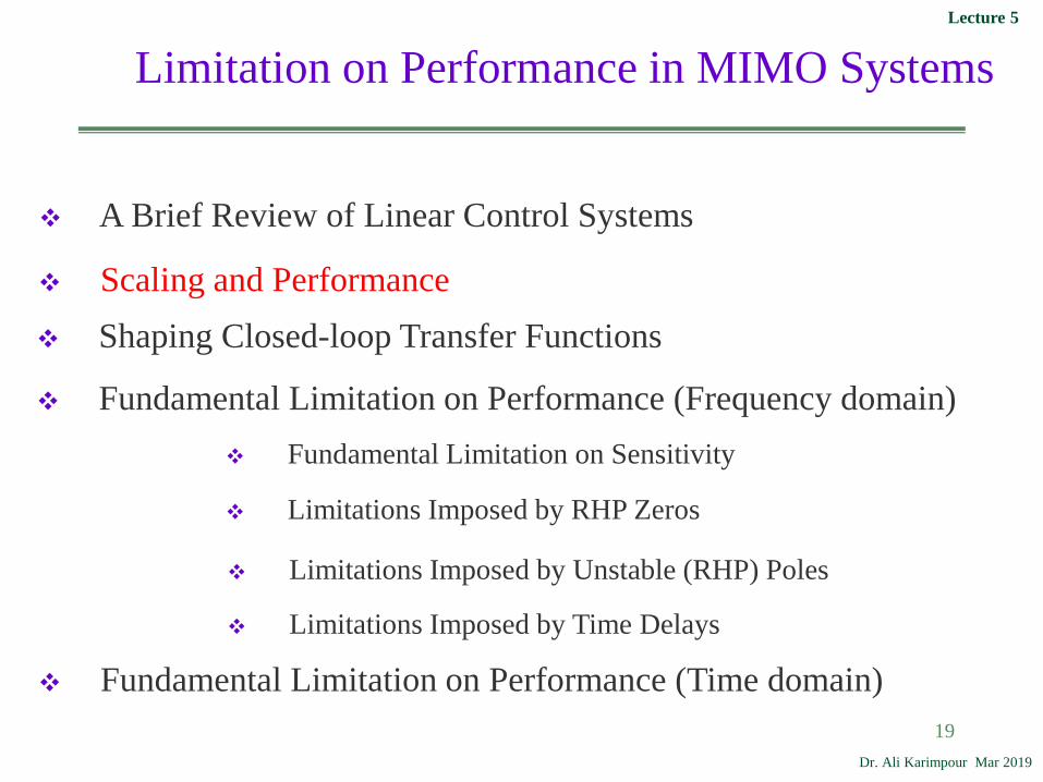
Limitation on Performance in MIMO Systems
Topics to be covered include:
Scaling and Performance
Shaping Closed-loop Transfer Functions
Fundamental Limitation on Sensitivity
Limitations Imposed by RHP Zeros
Limitations Imposed by Unstable (RHP) Poles
Limitations Imposed by Time Delays
Fundamental Limitation on Performance (Frequency domain)
Fundamental Limitation on Performance (Time domain)
A Brief Review of Linear Control Systems

Dr. Ali Karimpour Mar 2019
Lecture 5
3
A Brief Review of Linear Control Systems
Time Domain Performance
Frequency Domain Performance
Bandwidth and Crossover Frequency

Dr. Ali Karimpour Mar 2019
Lecture 5
4
Time Domain Performance
• Nominal stability NS: The system is stable with no model
uncertainty.
• Nominal Performance NP: The system satisfies the performance
specifications with no model uncertainty.
• Robust stability RS: The system is stable for all perturbed plants
about the nominal model up to the worst case model uncertainty.
• Robust performance RP: The system satisfies the performance
specifications for all perturbed plants about the nominal model up
to the worst case model uncertainty.

Dr. Ali Karimpour Mar 2019
Lecture 5
5
Time Domain Performance
The objective of this section is to discuss the ways of
evaluating closed loop performance.
Although closed loop stability is an important issue,
the real objective of control is to improve performance, that is,
to make the output y(t) behave in a more desirable manner.
Actually, the possibility of inducing instability is one of the
disadvantages of feedback control which has to be traded off
against performance improvement.

Dr. Ali Karimpour Mar 2019
Lecture 5
6
Time Domain Performance
Step response of a system
Rise time, tr Settling time, ts Overshoot, P.O
Decay ratio Steady state offset, ess
• ISE : Integral squared error deISE 2
0)(
• IAE : Integral absolute error deIAE
0
)(
• ITSE : Integral time weighted squared error deITSE 2
0)(
• ITAE : Integral time weighted absolutesquared error

Dr. Ali Karimpour Mar 2019
Lecture 5
7
Frequency Domain
Performance
Let L(s) denote the loop transfer
function of a system which is
closed-loop stable under negative
feedback.
Bode plot of )( jL
)(
1
180jLGM
180)( 180 jL
1)( cjL
180)( cjLPM
cPM /max
Nyquist plot of )( jL

Dr. Ali Karimpour Mar 2019
Lecture 5
8
Frequency Domain Performance
Stability margins are measures of how close a stable closed-loop system
is to instability.
From the above arguments we see that the GM and PM provide stability
margins for gain and delay uncertainty.
More generally, to maintain closed-loop stability, the Nyquist stability
condition tells us that the number of encirclements of the critical point
-1 by must not change. )( jL
Thus the actual closest distance to -1 is a measure of stability

Dr. Ali Karimpour Mar 2019
Lecture 5
9
Frequency Domain Performance
)(max
jSM s
Thus one may also view Ms as a robustness measure.
sM
1

Dr. Ali Karimpour Mar 2019
Lecture 5
10
Frequency Domain Performance
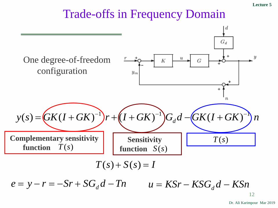
One degree-of-freedom
configuration
nGKIGKdGGKIrGKIGKsy d
111 )()()()(
Complementary sensitivity
function )(sTSensitivity
function )(sS
The maximum peaks of the sensitivity and complementary sensitivity
functions are defined as
)(max)(max
jTMjSM Ts

Dr. Ali Karimpour Mar 2019
Lecture 5
11
Frequency Domain Performance
There is a close relationship between MS and MT and the GM and PM.
][1
2
1sin2;
1
1 radMM
PMM
MGM
sss
s
][1
2
1sin2;
11 1 rad
MMPM
MGM
TTT
For example, with MS = 2 we are guaranteed GM > 2 and PM >29˚.
For example, with MT = 2 we are guaranteed GM > 1.5 and PM >29˚.
Dr. Ali Karimpour Mar 2019
Lecture 5
12
One degree-of-freedom
configuration
nGKIGKdGGKIrGKIGKsy d
111 )()()()(
Complementary sensitivity
function )(sTSensitivity
function )(sS
Trade-offs in Frequency Domain
)(sT
IsSsT )()(
TndSGSrrye d KSndKSGKSru d

Dr. Ali Karimpour Mar 2019
Lecture 5
13
Trade-offs in Frequency Domain
IsSsT )()(
TndSGSrrye d KSndKSGKSru d
1)()(
sLIsS
• Performance, good disturbance rejection LITS or or 0
• Performance, good command following LITS or or 0
• Mitigation of measurement noise on output 0or or 0 LIST
• Small magnitude of input signals 0Lor 0or 0 TK
• Physical controller must be strictly proper 0Tor 0or 0 LK
• Nominal stability (stable plant) small be L
• Stabilization of unstable plant ITL or large be

Dr. Ali Karimpour Mar 2019
Lecture 5
14
Bandwidth and Crossover Frequency
Definition 5-1
below. from db 3- crossesfirst )S(j
wherefrequency theis , ,bandwidth The B
Definition 5-2
above. from db 3- crosses )T(jat which
frequency highest theis , ,bandwidth The BT
Definition 5-3
above. from db 0 crosses )L(j where
frequency theis , ,frequency crossover gain The c
100
101
102
103
-60
-40
-20
0
20
40
60Singular Values
Frequency (rad/sec)
Sin
gula
r V
alu
es (
dB
)
L
T
S

Dr. Ali Karimpour Mar 2019
Lecture 5
15
Bandwidth and Crossover Frequency
Specifically, for systems with PM < 90˚ (most practical systems) we have
BTcB
In conclusion ωB ( which is defined in terms of S ) and also ωc
( in terms of L ) are good indicators of closed-loop performance,
while ωBT ( in terms of T ) may be misleading in some cases.
100
101
102
103
-60
-40
-20
0
20
40
60Singular Values
Frequency (rad/sec)
Sin
gula
r V
alu
es (
dB
)
L
T
S

Dr. Ali Karimpour Mar 2019
Lecture 5
16
Bandwidth and Crossover Frequency
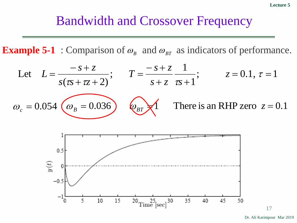
Example 5-1 : Comparison of and as indicators of performance.BTB
1,1.0;1
1;
)2(Let
z
szs
zsT
zss
zsL
036.0B054.0c 1BT 1.0 zero RHPan is There z
Dr. Ali Karimpour Mar 2019
Lecture 5
17
Bandwidth and Crossover Frequency
Example 5-1 : Comparison of and as indicators of performance.BTB
1,1.0;1
1;
)2(Let
z
szs
zsT
zss
zsL
036.0B054.0c 1BT 1.0 zero RHPan is There z

Dr. Ali Karimpour Mar 2019
Lecture 5
18
Introduction
One degree-of-freedom
configuration
nGKIGKdGGKIrGKIGKsy d
111 )()()()(
nsTdGsSrsTsy d )()()()(
• Performance, good disturbance rejection LITS or or 0
• Performance, good command following LSIT or 0or
• Mitigation of measurement noise on output 0or or 0 LIST
Dr. Ali Karimpour Mar 2019
Lecture 5
19
Limitation on Performance in MIMO Systems
Scaling and Performance
Shaping Closed-loop Transfer Functions
Fundamental Limitation on Sensitivity
Limitations Imposed by Time Delays
Limitations Imposed by RHP Zeros
Limitations Imposed by Unstable (RHP) Poles
Fundamental Limitation on Performance (Frequency domain)
Fundamental Limitation on Performance (Time domain)
A Brief Review of Linear Control Systems

Dr. Ali Karimpour Mar 2019
Lecture 5
20
Scaling
ryedGuGy dˆˆˆ;ˆˆˆˆˆ
rDreDeyDyuDudDd eeeudˆ,ˆ,ˆ,ˆ,ˆ 11111
rDyDeDdDGuDGyDeeeddue
;
ddedue DGDGDGDG ˆ,ˆ 11 ryedGGuy d ;

Dr. Ali Karimpour Mar 2019
Lecture 5
21
Shaping Closed-loop Transfer Functions
Many design procedure act on the shaping of the open-loop transfer
function L.
An alternative design strategy is to directly shape the magnitudes of
closed-loop transfer functions, such as S(s) and T(s).
Such a design strategy can be formulated as an H∞ optimal control
problem, thus automating the actual controller design and leaving
the engineer with the task of selecting reasonable bounds “weights”
on the desired closed-loop transfer functions.
Dr. Ali Karimpour Mar 2019
Lecture 5
22
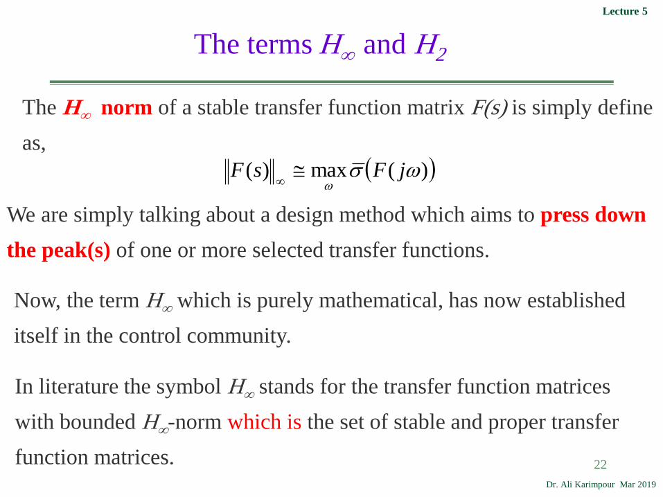
The terms H∞ and H2
The H∞ norm of a stable transfer function matrix F(s) is simply define
as,
)(max)(
jFsF
We are simply talking about a design method which aims to press down
the peak(s) of one or more selected transfer functions.
Now, the term H∞ which is purely mathematical, has now established
itself in the control community.
In literature the symbol H∞ stands for the transfer function matrices
with bounded H∞-norm which is the set of stable and proper transfer
function matrices.

Dr. Ali Karimpour Mar 2019
Lecture 5
23
The terms H∞ and H2
The H2 norm of a stable transfer function matrix F(s) is simply define
as,
djFjFtrsF H)()(
2
1)(
2
Similarly, the symbol H2 stands for the transfer function matrices with
bounded H2-norm, which is the set of stable and strictly proper transfer
function matrices.
Note that the H2 norm of a semi-proper transfer function is infinite,
whereas its H∞ norm is finite.
Why?

Dr. Ali Karimpour Mar 2019
Lecture 5
24
Weighted Sensitivity
As already discussed, the sensitivity function S is a very good indicator
of closed-loop performance (both for SISO and MIMO systems).
The main advantage of considering S is that because we ideally want
S to be small, it is sufficient to consider just its magnitude, ||S|| that is,
we need not worry about its phase.
Why S is a very good indicator of closed-loop performance in many
literatures?

Dr. Ali Karimpour Mar 2019
Lecture 5
25
Weighted Sensitivity
Typical specifications in terms of S include:
• Minimum bandwidth frequency ωB*.
• Maximum tracking error at selected frequencies.
• System type, or alternatively the maximum steady-state tracking
error, A.
• Shape of S over selected frequency ranges.
• Maximum peak magnitude of S, ||S(jω)||∞≤M
The peak specification prevents amplification of noise at high frequencies,
and also introduces a margin of robustness; typically we select M=2

Dr. Ali Karimpour Mar 2019
Lecture 5
26
Weighted Sensitivity
)(
1
swp
,)(
1)(
jwjS
P
Mathematically, these specifications may be captured simply by an
upper bound
1)()(,1)()(
jSjwjSjw PP
The subscript P stands for performance

Dr. Ali Karimpour Mar 2019
Lecture 5
27
Weight Selection
As
Mssw
B
BP
/)(
plot of )(
1
jwP
Performance at Low Frequencies

Dr. Ali Karimpour Mar 2019
Lecture 5
28
Weight Selection
Performance at High Frequencies
plot of )(
1
jwP
B
P
s
Msw
1)(

Dr. Ali Karimpour Mar 2019
Lecture 5
29
Weight Selection
A weight which asks for a slope -2 for L at lower frequencies is
22/1
22/1/
)(As
Mssw
B
BP
The insight gained from the previous section on loop-shaping design
is very useful for selecting weights.
For example, for disturbance rejection
1)( jSGd
It then follows that a good initial choice for the performance weight is
to let wP(s) look like |Gd(jω)| at frequencies where |Gd(jω)| >1

Dr. Ali Karimpour Mar 2019
Lecture 5
30
Weighted Sensitivity

Dr. Ali Karimpour Mar 2019
Lecture 5
31
Stacked Requirements: Mixed Sensitivity
The specification ||wPS||∞<1 puts a lower bound on the bandwidth,
but not an upper one, and nor does it allow us to specify the roll-off
of L(s) above the bandwidth.
To do this one can make demands on another closed-loop transfer
function
KSw
Tw
Sw
NjNN
u
T
P
,1)(max
For SISO systems, N is a vector and
222)( KSwTwSwN uTP

Dr. Ali Karimpour Mar 2019
Lecture 5
32
Solving H∞ Optimal Control Problem
After selecting the form of N and the weights, the H∞ optimal controller
is obtained by solving the problem
)(min KN
K
Let denote the optimal H∞ norm. )(min0 KN
K
The practical implication is that, except for at most a factor the
transfer functions will be close to times the bounds selected by
the designer.
n
0
This gives the designer a mechanism for directly shaping the magnitudes of
)( and )( , )( KSTS

Dr. Ali Karimpour Mar 2019
Lecture 5
33
Solving H∞ Optimal Control Problem
Example 5-2110
100)(,
)105.0(
1
110
200)(
2
ssG
sssG d
The control objectives are:
1. Command tracking: The rise time (to reach 90% of the final value)
should be less than 0.3 second and the overshoot should be less than 5%.
2. Disturbance rejection: The output in response to a unit step disturbance
should remain within the range [-1,1] at all times, and it should return to 0
as quickly as possible (|y(t)| should at least be less than 0.1 after 3 seconds).
3. Input constraints: u(t) should remain within the range [-1,1] at all times
to avoid input saturation (this is easily satisfied for most designs).
Dr. Ali Karimpour Mar 2019
Lecture 5
34
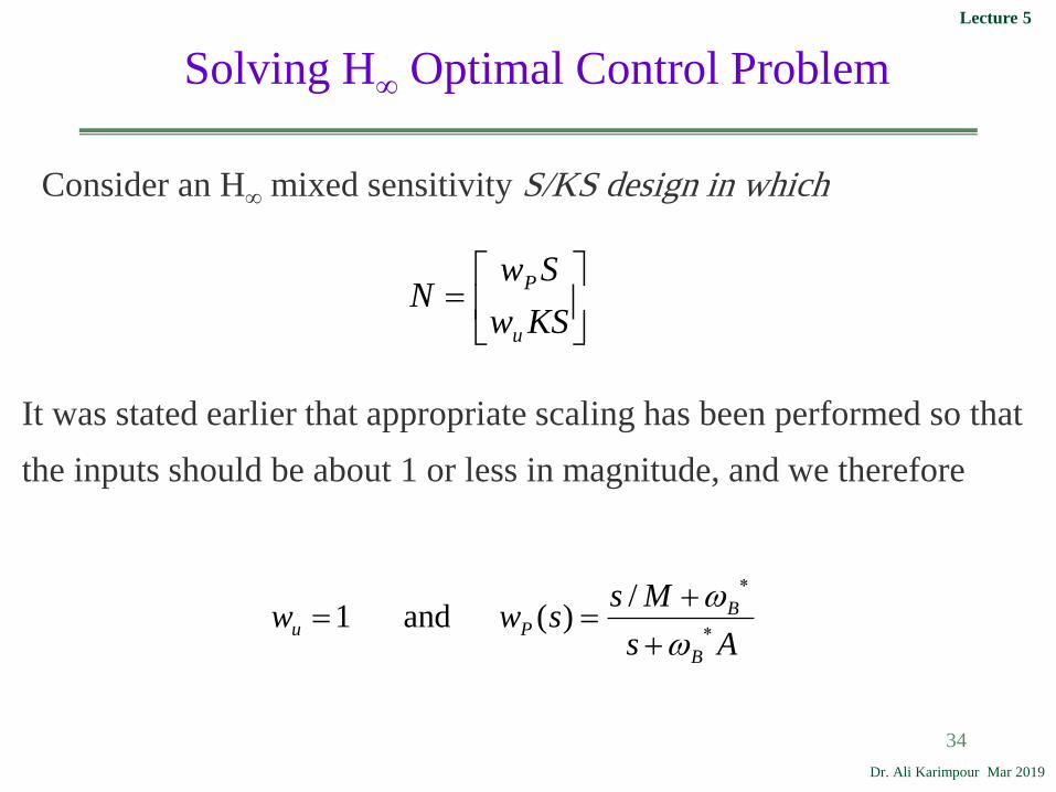
Solving H∞ Optimal Control Problem
Consider an H∞ mixed sensitivity S/KS design in which
KSw
SwN
u
P
It was stated earlier that appropriate scaling has been performed so that
the inputs should be about 1 or less in magnitude, and we therefore
As
Mssww
B
BPu
/)( and 1

Dr. Ali Karimpour Mar 2019
Lecture 5
35
Solving H∞ Optimal Control Problem
110
100)(of diagram Bode theSee
ssGd
-20
-10
0
10
20
30
40
Magnitu
de (
dB
)
10-3
10-2
10-1
100
101
102
-90
-45
0
Phase (
deg)
Bode Diagram
Frequency (rad/sec)
We need control till 10 rad/sec to reduce disturbance and a suitable rise time.
sec/10 let So radcB
Overshoot should be less than 5% so let MS<1.5

Dr. Ali Karimpour Mar 2019
Lecture 5
36
Solving H∞ Optimal Control Problem
410,10,5.1,/
)(
AM
As
Mssw B
B
BP
For this problem, we achieved an optimal H∞ norm of 1.37, so the
weighted sensitivity requirements are not quite satisfied. Nevertheless,
the design seems good with
rad/sec 22.5 and 2.71,04.8,0.1,30.1 cTS PMGMMM

Dr. Ali Karimpour Mar 2019
Lecture 5
37
Solving H∞ Optimal Control Problem
The tracking response is very good as shown by curve in Figure.
However, we see that the disturbance response is very sluggish.

Dr. Ali Karimpour Mar 2019
Lecture 5
38
Solving H∞ Optimal Control Problem
If disturbance rejection is the main concern, then from our earlier
discussion we need for a performance weight that specifies higher
gains at low frequencies. We therefore try
6
22/1
22/1
10,10,5.1,/
)(
AM
As
Mssw B
B
BP
For this problem, we achieved an optimal H∞ norm of 2.21, so the
weighted sensitivity requirements are not quite satisfied. Nevertheless,
the design seems good with
rad/sec 2.11 and 3.43,76.4,43.1,63.1 c PMGMMM TS

Dr. Ali Karimpour Mar 2019
Lecture 5
39
Solving H∞ Optimal Control Problem

Dr. Ali Karimpour Mar 2019
Lecture 5
40
Limitation on Performance in MIMO Systems
Scaling and Performance
Shaping Closed-loop Transfer Functions
Fundamental Limitation on Sensitivity
Limitations Imposed by Time Delays
Limitations Imposed by RHP Zeros
Limitations Imposed by Unstable (RHP) Poles
Fundamental Limitation on Performance (Frequency domain)
Fundamental Limitation on Performance (Time domain)
A Brief Review of Linear Control Systems

Dr. Ali Karimpour Mar 2019
Lecture 5
41
Fundamental Limitation on Sensitivity
(Frequency domain)
S plus T is the identity matrix
ITS
1)()(1)( STS
1)()(1)( TST

Dr. Ali Karimpour Mar 2019
Lecture 5
42
Interpolation ConstraintsRHP-zero:
If G(s) has a RHP-zero at z with output direction yz then for internal stability
of the feedback system the following interpolation constraints must apply:
In MIMO Case:H
z
H
z
H
z yzSyzTy )(;0)(
In SISO Case: 1)(;0)( zSzT
0)( zGyH
z
Proof:
0)( zLyH
z LST
0)( zTyH
z0))(( zSIy
H
z
S has no RHP-pole
Fundamental Limitation on Sensitivity
(Frequency domain)

Dr. Ali Karimpour Mar 2019
Lecture 5
43
Limitations Imposed by RHP Zeros
Moving the Effect of a RHP-zero to a Specific Output
Example 5-3
221
11
)1)(12.0(
1)(
ssssG
which has a RHP-zero at s = z = 0.5
The output zero direction is
45.0
89.0
1
2
5
1zy
Interpolation constraint is
0)()(2;0)()(2 22122111 ztztztzt

Dr. Ali Karimpour Mar 2019
Lecture 5
44
Limitations Imposed by RHP Zeros
Moving the Effect of a RHP-zero to a Specific Output
0)()(2;0)()(2 22122111 ztztztzt
zs
zszs
zs
sT
0
0)(0
???01
)( 11
zs
zs
zs
ssT 41
45.0
89.0zy
???
10
)(2
2
zs
s
zs
zs
sT
12

Dr. Ali Karimpour Mar 2019
Lecture 5
45
Limitations Imposed by RHP Zero
Theorem 5-1 Assume that G(s) is square, functionally controllable and stable
and has a single RHP-zero at s = z and no RHP-pole at s = z. Then if the k’th
Element of the output zero direction is non-zero, i.e. yzk ≠ 0 it is possible to
obtain “perfect” control on all outputs j ≠ k with the remaining output
exhibiting no steady-state offset. Specifically, T can be chosen of the form
1...000...00
............
............
......
............
............
0...000...10
0...000...01
)(1121
zs
s
zs
s
zs
zs
zs
s
zs
s
zs
ssTnkk kjfor
y
y
zk
zj
j 2

Dr. Ali Karimpour Mar 2019
Lecture 5
46
Interpolation ConstraintsRHP-pole:
If G(s) has a RHP pole at p with output direction yp then for internal
stability the following interpolation constraints apply
In MIMO Case: ppp yypTypS )(;0)(
In SISO Case: 1)(;0)( pTpS
Proof:
0)(1
pypL SLT T has no RHP-pole S has a RHP-zero
1 TLS 0)()()( 1
pp ypSypLpT ppp yypSIypT )()(
Fundamental Limitation on Sensitivity
(Frequency domain)
Dr. Ali Karimpour Mar 2019
Lecture 5
47
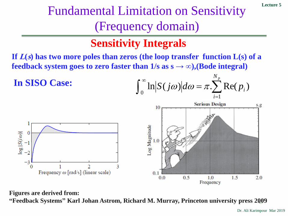
Sensitivity Integrals
pN
i
ipdjS1
0)Re(.)(ln
If L(s) has two more poles than zeros (the loop transfer function L(s) of a
feedback system goes to zero faster than 1/s as s → ∞),(Bode integral)
Fundamental Limitation on Sensitivity
(Frequency domain)
In SISO Case:
Figures are derived from:
“Feedback Systems” Karl Johan Astrom, Richard M. Murray, Princeton university press 2009

Dr. Ali Karimpour Mar 2019
Lecture 5
48
Sensitivity Integrals
pN
i
i
i
i pdjSdjS1
00)Re(.)(ln)(detln
pN
i
ipdjS1
0)Re(.)(ln
If L(s) has two more poles than zeros (the loop transfer function L(s) of a
feedback system goes to zero faster than 1/s as s → ∞),(Bode integral)
In MIMO Case: (Generalization of SISO case)
Fundamental Limitation on Sensitivity
(Frequency domain)
In SISO Case:

Dr. Ali Karimpour Mar 2019
Lecture 5
49
Fundamental Limitation: Bounds on Peaks
TMSM TS min,min min,min,
In the following, MS,min and MT,min denote the lowest achievable values
for ||S||∞ and ||T||∞ , respectively, using any stabilizing controller K.

Dr. Ali Karimpour Mar 2019
Lecture 5
50
Fundamental Limitation: Bounds on Peaks
Theorem 5-2 Sensitivity and Complementary Sensitivity Peaks
Consider a rational plant G(s) (with no time delay). Suppose G(s) has Nz
RHP-zeros with output zero direction vectors yz,i and Np RHP-poles with
output pole direction vectors yp,i. Suppose all zi and pi are distinct.
Then we have the following tight lower bound on ||T||∞ and ||S||∞
2/12/12
min,min, 1
pzpzTS QQQMM
ji
jp
H
iz
ijzp
ji
jp
H
ip
ijp
ji
jz
H
iz
ijzpz
yyQ
pp
yyQ
zz
yyQ
,,,,,,,,

Dr. Ali Karimpour Mar 2019
Lecture 5
51
Fundamental Limitation: Bounds on Peaks
Example 5-4
2)1)(2(
)3)(1()(
ss
sssG
Derive lower bounds on ||T||∞ and ||S||∞
2,3,1 121 pzz
1
1,4/1,
6/14/1
4/12/1, pzpz QQQ
156786.12
9531.71 2
min,min,
TS MM
Dr. Ali Karimpour Mar 2019
Lecture 5
52
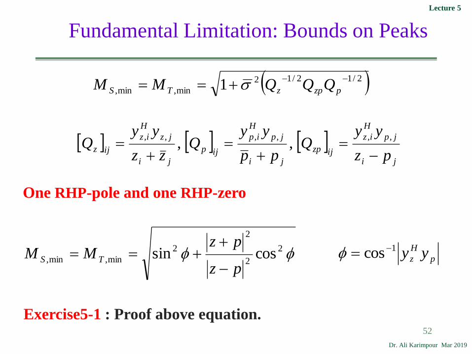
Fundamental Limitation: Bounds on Peaks
2/12/12
min,min, 1
pzpzTS QQQMM
ji
jp
H
iz
ijzp
ji
jp
H
ip
ijp
ji
jz
H
iz
ijzpz
yyQ
pp
yyQ
zz
yyQ
,,,,,,,,
One RHP-pole and one RHP-zero
2
2
2
2
min,min, cossinpz
pzMM TS
p
H
z yy1cos
Exercise5-1 : Proof above equation.

Dr. Ali Karimpour Mar 2019
Lecture 5
53
Fundamental Limitation: Bounds on Peaks
Example 5-5
3,2;
11.0
20
011.0
cossin
sincos
3
10
01
)(
pz
s
ss
zs
s
pssG
U
)3)(11.0(
20
0))(11.0(
)(,10
0100
ss
s
pss
zs
sGandU
0)3)(11.0(
))(11.0(
20
)(,01
109090
ss
zs
pss
s
sGandU

Dr. Ali Karimpour Mar 2019
Lecture 5
54
Fundamental Limitation: Bounds on Peaks
5.0,2,/
,
BB
Pu MIs
MsWIW

Dr. Ali Karimpour Mar 2019
Lecture 5
55
Fundamental Limitation: Bounds on Peaks
The corresponding responses to a step change in the reference r = [ 1 -1 ] , are shown
Solid line: y1
Dashed line: y2
1- For α = 0 there is one RHP-pole and zero so the responses for y1 is very poor.
2- For α = 90 the RHP-pole and zero do not interact but y2 has an undershoot since of …
3- For α = 0 and 30 the H∞ controller is unstable since of …

Dr. Ali Karimpour Mar 2019
Lecture 5
56
Limitations Imposed by RHP Zeros
The limitations of a RHP-zero located at z may also be derived from
the bound (by maximum module theorem)
)())((.)(max)()( zwjSjwsSsw PPP
1)()(
sSswP1)( zwP

Dr. Ali Karimpour Mar 2019
Lecture 5
57
Limitations Imposed by RHP Zeros
Performance at Low Frequencies 1)()(
sSswP
1)( zwP
As
Mssw
B
BP
/)( 1
/)(
Az
Mzzw
B
BP
Real zero: )(2
Iz
B
Imaginary zero
)1
1()1(M
zAB
)(87.0 IIzB
2
11
MzB
Exercise5-2 : Derive (I) and (II).

Dr. Ali Karimpour Mar 2019
Lecture 5
58
Limitations Imposed by RHP Zeros
Performance at High Frequencies 1)()(
sSswP
1)( zwP
11
)(
B
P
z
Mzw
Real zero: zB 2
B
P
s
Msw
1)(
MzB
/11
1
B
P
s
Msw
1)(

Dr. Ali Karimpour Mar 2019
Lecture 5
59
Limitations Imposed by Unstable (RHP) Poles
)())((.)(max)()( pwjTjwsTsw TTT
1)()(
sTswT1)( pwT
TBT
TM
ssw
1)(
Real RHP-pole
1
T
TBT
M
Mp pBT 2
Imaginary RHP-pole pBT 15.1
pc 2

Dr. Ali Karimpour Mar 2019
Lecture 5
60
Limitations Imposed by Time Delays
ijj
i minmin
A lower bound on the time delay for output i is given by the smallest
delay in row i of G(s)
For MIMO systems we have the surprising result that an increased time
delay may sometimes improve the achievable performance. As a simple
example, consider the plant
1
11)(
sesG

Dr. Ali Karimpour Mar 2019
Lecture 5
61
Limitation on Performance in MIMO Systems
Scaling and Performance
Shaping Closed-loop Transfer Functions
Fundamental Limitation on Sensitivity
Limitations Imposed by Time Delays
Limitations Imposed by RHP Zeros
Limitations Imposed by Unstable (RHP) Poles
Fundamental Limitation on Performance (Frequency domain)
Fundamental Limitation on Performance (Time domain)

Dr. Ali Karimpour Mar 2019
Lecture 5
62
Fundamental Limitation on Performance
(Time domain)
Reference: “Interaction Bounds in Multivariable Control Systems” K H Johanson,
Automatica, vol 38,pp 1045-1051, 2002
Consider the system:
)()()()(
)()()(
sYsRsCsU
sUsGsY
Let a step response signal at
i th input but other inputs are zero so
)(ˆ tur
0),()(sup0
trtyy iit
o
i
Undershoot is
defined as: 0),(sup
0
tyy it
u
i
)(supˆ0
tyy kt
ki
Overshoot in
output i is:
Settling time is defined as:
ttrtyt kk
mksi ,)()(:infmax
0,...,1
Rise time is defined as:

Dr. Ali Karimpour Mar 2019
Lecture 5
63
Fundamental Limitation on Performance
(Time domain)Theorem5-3: Consider the stable closed loop system with zero initial conditions at
t=0 and let for t>0. Assume that the open loop transfer function
G has a real RHP zero z > 0 with zero direction yz and yz1 >0. then we have:
Trtr 0,...,0,ˆ)(
m
k
zkzzt
m
k
kzk
u
z yrye
yyyys
2
1
2
111 )ˆ(1
1ˆ
1
undershoot
interaction settling time settling levelelements of
zero direction
Theorem5-4: Consider the stable closed loop system with zero initial conditions at
t=0. Assume that the open loop transfer function G has a real RHP pole p > 0 with
pole direction yp and yp1 >0. Consider m independent responses with for
t>0. Then we have:
rtriˆ)(
m
k
kpk
pt
pr
m
k
kpk
o
p yyeyptr
yyyy r
2
111
2
111ˆ1
2
ˆˆ 1
overshoot
interaction rise timeelements of
pole direction

Dr. Ali Karimpour Mar 2019
Lecture 5
64
Fundamental Limitation on Performance
(Time domain)
Example5-6: Experimental set-up for the quadruple-tank process.

Dr. Ali Karimpour Mar 2019
Lecture 5
65
Fundamental Limitation on Performance
(Time domain)
Example5-6(Continue): Experimental set-up for the quadruple-tank process.
pointset valve:1
Input#1
Pump1
Input#2
Pump2
Output#1 Output#2
pointset valve:2
Valve set points are used to make the
process more or less difficult to control.
6.0,7.0 here zero, RHP no 2,1 If 2121
1
11
sss
ssssG
67.981
24.3
)67.981)(90.381(
71.1
)57.951)(05.321(
04.2
57.951
11.3
)(
045.0012.0 21 zz
34.0,43.0 here zero, RHP one 1,0 If 2121
sss
ssssG
55.1111
97.1
)55.1111)(3.561(
11.3
)75.761)(30.521(
33.3
75.761
69.1
)(
051.0014.0 21 zz

Dr. Ali Karimpour Mar 2019
Lecture 5
66
Fundamental Limitation on Performance
(Time domain)
High undershoot for small interaction.
For a unit step in r1 we have:
For a settling time of ts1=100 we have:

Dr. Ali Karimpour Mar 2019
Lecture 5
67
Fundamental Limitation on Performance
(Time domain)

Dr. Ali Karimpour Mar 2019
Lecture 5
68
Fundamental Limitation on Performance
(Time domain)

Dr. Ali Karimpour Mar 2019
Lecture 5
Exercises
69
5-3 Consider the following weight with f>1.
5-4 Consider the weight
5-1 Mentioned in the lecture.
5-2 Mentioned in the lecture.

Dr. Ali Karimpour Mar 2019
Lecture 5
Exercises (Continue)
70
5-5 Consider the plant
5-6 Repeat 5-5 for following plant.

Dr. Ali Karimpour Mar 2019
Lecture 5
71
References
• Control Configuration Selection in Multivariable Plants, A. Khaki-Sedigh, B. Moaveni, Springer Verlag, 2009.
References
• Multivariable Feedback Control, S.Skogestad, I. Postlethwaite, Wiley,2005.
• Multivariable Feedback Design, J M Maciejowski, Wesley,1989.
• http://saba.kntu.ac.ir/eecd/khakisedigh/Courses/mv/
Web References
• http://www.um.ac.ir/~karimpor
• تحليل و طراحی سيستم های چند متغيره، دکتر علی خاکی صديق