multiple regression variable selection - new york...

≈≈≈≈≈ MULTIPLE REGRESSION VARIABLE SELECTION ≈≈≈≈≈

1

MULTIPLE REGRESSION VARIABLE SELECTION

Documents prepared for use in course B01.1305, New York University, Stern School of Business

A simple example of variable selection page 3 This example explores the prices of n = 61 condominium units. The model simplifies directly by using the only predictor that has a significant t statistic. It doesn’t get any simpler than this.

Collinearity page 7 Collinearity is the curse of multiple regression. Here are some clues for detecting collinearity and also some cures (Cp , stepwise regression, best subsets regression).

Example on housing prices page 12 This example involves home prices in a suburban subdivision. It illustrates the use of indicator variables, as well as variable selection. It shows an example of a regression prediction, illustrating the point that it can be destructive to make predictions using all available independent variables.

Hypothesis tests of regression page 14 There are many hypothesis tests associated with multiple regression, and these are explained here. There is also commentary about predictions. Please see the caveat regarding compromised inferences after any variable selection process.

An example of variable selection page 18 This example, trash hauling data, shows stepwise regression.

≈≈≈≈≈ MULTIPLE REGRESSION VARIABLE SELECTION ≈≈≈≈≈

2

Variable selection on the condominium units (reprise) page 22

The problem illustrated on page 3 is revisited, but with a larger sample size n = 209. The larger sample size makes it possible to find more significant effects. At the end, this illustrates some neat detective work to extract a quadratic effect.

Example with brutal collinearity page 27 This example, on college library expenses, shows very intense collinearity.

Strategy for variable selection page 31 Here are a number of steps that should help with the variable selection problem.

Cover photo: Sunken Meadow Park, Long Island Last edit date: 7 APR 2008 © Gary Simon, 2008

A SIMPLE EXAMPLE OF VARIABLE SELECTION

3

This uses a data set involving prices of 61 condominium units within a Florida development. The data set is taken from Mendenhall and Sinsich (the original source has n = 209). These data are on the Stern network in file X:\SOR\B011305\M\CONDO.MTP. The variables here are

PRICE = selling price of condo unit FLOOR = floor (1 to 8) DELEV = distance from elevator (units unclear; could be yards) VIEW = 1 if view of ocean, 0 otherwise END = 1 if end unit, 0 otherwise FURN = 1 if furnished, 0 otherwise

The objective here will be to relate the obvious dependent variable PRICE to the other variables. The variables VIEW, END, and FURN are called dummy (or indicator) variables because they take only two values. The regression model is

PRICEi = β0 + βFLOOR FLOORi + βDELEV DELEVi + βVIEW VIEWi

+ βEND ENDi + βFURN FURNi + εi

where i = 1, 2, 3, ..., n (Here n = 61.) Note that the coefficients of dummy variables have an immediate and obvious interpretation:

βVIEW represents the added value of an ocean view βEND represents the added value of an end unit βFURN represents the added value of furniture

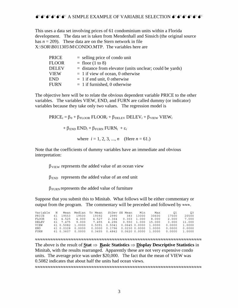
Suppose that you submit this to Minitab. What follows will be either commentary or output from the program. The commentary will be preceded and followed by ≈≈≈. Variable N Mean Median Tr Mean StDev SE Mean Min Max Q1 Q3 PRICE 61 19553 19500 19392 2990 383 13000 30600 17500 20500 FLOOR 61 4.525 4.000 4.527 2.364 0.303 1.000 8.000 2.000 7.000 DELEV 61 7.475 9.000 7.455 4.296 0.550 1.000 15.000 3.000 11.000 VIEW 61 0.5082 1.0000 0.5091 0.5041 0.0645 0.0000 1.0000 0.0000 1.0000 END 61 0.0328 0.0000 0.0000 0.1796 0.0230 0.0000 1.0000 0.0000 0.0000 FURN 61 0.3607 0.0000 0.3455 0.4842 0.0620 0.0000 1.0000 0.0000 1.0000

≈≈≈≈≈≈≈≈≈≈≈≈≈≈≈≈≈≈≈≈≈≈≈≈≈≈≈≈≈≈≈≈≈≈≈≈≈≈≈≈≈≈≈≈≈≈≈≈≈≈≈≈≈≈≈≈≈≈≈≈≈≈≈≈≈ The above is the result of Stat ⇒ Basic Statistics ⇒ Display Descriptive Statistics in Minitab, with the results rearranged. Apparently these are not very expensive condo units. The average price was under $20,000. The fact that the mean of VIEW was 0.5082 indicates that about half the units had ocean views. ≈≈≈≈≈≈≈≈≈≈≈≈≈≈≈≈≈≈≈≈≈≈≈≈≈≈≈≈≈≈≈≈≈≈≈≈≈≈≈≈≈≈≈≈≈≈≈≈≈≈≈≈≈≈≈≈≈≈≈≈≈≈≈≈≈


4

Correlations (Pearson) PRICE FLOOR DELEV VIEW END FLOOR -0.211 DELEV 0.152 -0.035 VIEW 0.619 -0.158 -0.021 END -0.065 0.037 -0.064 0.181 FURN 0.167 0.109 -0.204 0.124 0.053 ≈≈≈≈≈≈≈≈≈≈≈≈≈≈≈≈≈≈≈≈≈≈≈≈≈≈≈≈≈≈≈≈≈≈≈≈≈≈≈≈≈≈≈≈≈≈≈≈≈≈≈≈≈≈≈≈≈≈≈≈≈≈≈≈≈ The correlations matrix was generated by Stat ⇒ Basic Statistics ⇒ Correlations . Apparently the only strong correlation with PRICE is VIEW. ≈≈≈≈≈≈≈≈≈≈≈≈≈≈≈≈≈≈≈≈≈≈≈≈≈≈≈≈≈≈≈≈≈≈≈≈≈≈≈≈≈≈≈≈≈≈≈≈≈≈≈≈≈≈≈≈≈≈≈≈≈≈≈≈≈ Regression Analysis The regression equation is PRICE = 17187 - 149 FLOOR + 126 DELEV + 3654 VIEW - 2815 END + 920 FURN Predictor Coef StDev T P Constant 17187.4 944.8 18.19 0.000 FLOOR -148.5 127.2 -1.17 0.248 DELEV 125.96 69.94 1.80 0.077 VIEW 3654.1 606.6 6.02 0.000 END -2815 1670 -1.69 0.098 FURN 919.6 629.2 1.46 0.150 S = 2274 R-Sq = 46.9% R-Sq(adj) = 42.1% Analysis of Variance Source DF SS MS F P Regression 5 251757494 50351499 9.73 0.000 Error 55 284531883 5173307 Total 60 536289377 Source DF Seq SS FLOOR 1 23858715 DELEV 1 11312898 VIEW 1 191130106 END 1 14407311 FURN 1 11048464 Unusual Observations Obs FLOOR PRICE Fit StDev Fit Residual St Resid 28 3.00 18000 18337 1652 -337 -0.22 X 46 7.00 19000 18663 1652 337 0.22 X 54 5.00 13000 17616 670 -4616 -2.12R 61 3.00 30600 23205 836 7395 3.50R R denotes an observation with a large standardized residual X denotes an observation whose X value gives it large influence.


5

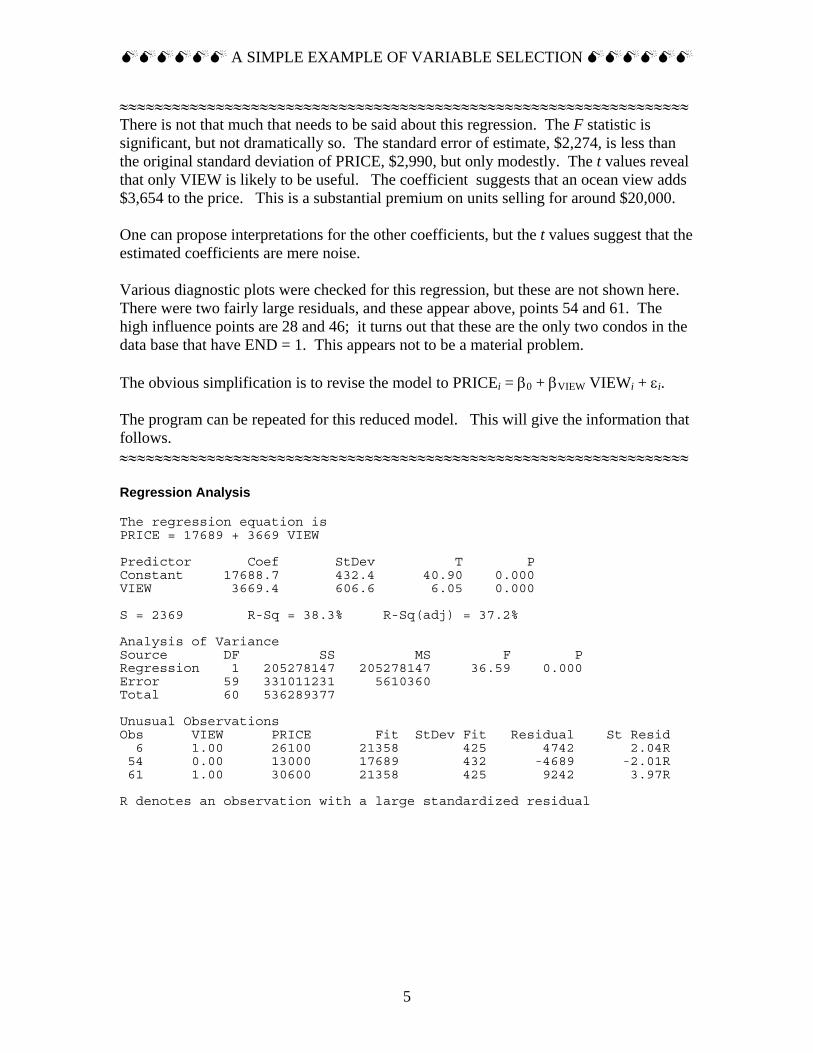
≈≈≈≈≈≈≈≈≈≈≈≈≈≈≈≈≈≈≈≈≈≈≈≈≈≈≈≈≈≈≈≈≈≈≈≈≈≈≈≈≈≈≈≈≈≈≈≈≈≈≈≈≈≈≈≈≈≈≈≈≈≈≈≈≈ There is not that much that needs to be said about this regression. The F statistic is significant, but not dramatically so. The standard error of estimate, $2,274, is less than the original standard deviation of PRICE, $2,990, but only modestly. The t values reveal that only VIEW is likely to be useful. The coefficient suggests that an ocean view adds $3,654 to the price. This is a substantial premium on units selling for around $20,000. One can propose interpretations for the other coefficients, but the t values suggest that the estimated coefficients are mere noise. Various diagnostic plots were checked for this regression, but these are not shown here. There were two fairly large residuals, and these appear above, points 54 and 61. The high influence points are 28 and 46; it turns out that these are the only two condos in the data base that have END = 1. This appears not to be a material problem. The obvious simplification is to revise the model to PRICEi = β0 + βVIEW VIEWi + εi. The program can be repeated for this reduced model. This will give the information that follows. ≈≈≈≈≈≈≈≈≈≈≈≈≈≈≈≈≈≈≈≈≈≈≈≈≈≈≈≈≈≈≈≈≈≈≈≈≈≈≈≈≈≈≈≈≈≈≈≈≈≈≈≈≈≈≈≈≈≈≈≈≈≈≈≈≈ Regression Analysis The regression equation is PRICE = 17689 + 3669 VIEW Predictor Coef StDev T P Constant 17688.7 432.4 40.90 0.000 VIEW 3669.4 606.6 6.05 0.000 S = 2369 R-Sq = 38.3% R-Sq(adj) = 37.2% Analysis of Variance Source DF SS MS F P Regression 1 205278147 205278147 36.59 0.000 Error 59 331011231 5610360 Total 60 536289377 Unusual Observations Obs VIEW PRICE Fit StDev Fit Residual St Resid 6 1.00 26100 21358 425 4742 2.04R 54 0.00 13000 17689 432 -4689 -2.01R 61 1.00 30600 21358 425 9242 3.97R R denotes an observation with a large standardized residual


6

≈≈≈≈≈≈≈≈≈≈≈≈≈≈≈≈≈≈≈≈≈≈≈≈≈≈≈≈≈≈≈≈≈≈≈≈≈≈≈≈≈≈≈≈≈≈≈≈≈≈≈≈≈≈≈≈≈≈≈≈≈≈≈≈≈ The F statistic is now quite impressive (since it is no longer diluted with worthless information). The standard error of estimate, $2,368, is almost as good as that of the previous more complicated run. The fitted model is PRÎCE = $17,689 + $3,669 VIEW , which suggests that an ocean view is worth $3,669. Please note the following comparisons:

Calculation Using no predictors Using 5 predictors Using VIEW alone sε 2,990 = sY 2,274 2,369 R2 0.0% 46.9% 38.3%

The best values for sε and R2 occur when all available predictors are used. The model using all predictors is needlessly complicated. We are much better off using a simpler model with values for sε and R2 that are not quite so strong.

The best statistic for choosing an appropriate model is almost certainly the Cp statistic. This will be discussed elsewhere.

The various diagnostic plots show no pathologies, so we stop here. ≈≈≈≈≈≈≈≈≈≈≈≈≈≈≈≈≈≈≈≈≈≈≈≈≈≈≈≈≈≈≈≈≈≈≈≈≈≈≈≈≈≈≈≈≈≈≈≈≈≈≈≈≈≈≈≈≈≈≈≈≈≈≈≈≈

COLLINEARITY

7

Collinearity in multiple regression refers to a condition in which dependencies among the independent variables make it difficult to reach a clean conclusion. Consider the following situation, involving dependent variable Y and four independent variables A, B, C, D. The data set has 70 points. Here are some quick descriptive statistics (edited from Minitab output):

Descriptive Statistics: A, B, C, D, Y Variable N Mean Median StDev A 70 200.12 200.15 30.24 B 70 176.92 176.65 27.62 C 70 70.67 71.95 11.03 D 70 53.021 52.400 7.548 Y 70 295.78 293.35 32.44

Plots of these variables were inspected, and none of these variables need to be transformed. Note that the standard deviation of Y, the dependent variable, is 32.44. Here are the correlations:

Correlations: A, B, C, D, Y A B C D B 0.997 C 0.597 0.539 D 0.761 0.712 0.962 Y 0.932 0.937 0.457 0.631

We find reasonably large correlations with Y (which is pleasing), but we also find some large correlations among A, B, C, and D (not so pleasing). Let’s try the regression. The information that follows is edited from the output of Minitab’s Stat ⇒ Regression ⇒ Regression .

Regression Analysis: Y versus A, B, C, D The regression equation is Y = 109 + 2.72 A - 1.63 B - 0.375 C - 0.81 D Predictor Coef SE Coef T P VIF Constant 109.20 10.03 10.89 0.000 A 2.721 1.494 1.82 0.073 1115.7 B -1.631 1.506 -1.08 0.283 946.4 C -0.3748 0.7130 -0.53 0.601 33.8 D -0.809 1.442 -0.56 0.577 64.7 S = 11.2346 R-Sq = 88.7% R-Sq(adj) = 88.0%

COLLINEARITY

8

This regression is pleasing on a number of grounds. We see that sε = 11.23 (much less that SD(Y) = 32.44) and R2 = 88.7%. However, none of the predictors are significant; each has a p-value larger than 0.05. Something funny is going on. The clue lies in the very large VIF values. These VIFs tell you to what extend a predictor is linearly dependent on other predictors. We like these to be close to 1, and we certainly get upset when they exceed 10.

VIF stands for variance inflation factor. The lowest possible value is 1.0, which is considered good. High values represent trouble, in that a variable with high VIF is likely to be strongly linearly dependent on other independent variables.

A related concept is the TOLERANCE, which is provided by some other software. The

quantities are related as VIF = 1TOLERANCE

. TOLERANCE values are between 0 (bad)

and 1 (good). For this problem, the TOLERANCE for variable A is defined as

TOLERANCE(A) = 1 - R2 (regression of A on B, C, D) Similarly, the TOLERANCE for variable B is

TOLERANCE(B) = 1 - R2 (regression of B on A, C, D) Thus, we’ve got a good regression with some problems. The likely possibility is that there are some strong dependencies among A, B, C, and D, since each has a large VIF number. There are several strategies that can be used. One is to remove independent variables one at a time until the VIF values for the variables remaining are all acceptable. This works well, but many people like to use an automated method. Minitab employs two automated methods, stepwise regression and best subset regression.

The best subsets option will by default list the two best models for each level of complexity. You will likely find it easier to just list one. You can fix this by Stat ⇒ Regression ⇒ Best Subsets ⇒ [ Options ⇒ [ Models of each size to print: 1 OK ⇒ ] OK ].

Here is the best subsets regression output for our problem:

Best Subsets Regression: Y versus A, B, C, D Response is Y Mallows Vars R-Sq R-Sq(adj) C-p S A B C D 1 87.8 87.6 4.4 11.428 X 2 88.5 88.2 2.2 11.166 X X 3 88.7 88.1 3.3 11.173 X X X 4 88.7 88.0 5.0 11.235 X X X X

COLLINEARITY

9

This tells you that the best model using one independent variable is the regression of Y on B, the best using two independent variables is Y on (A, C), and so on. If you’d like to see the details of those regressions, you’ve got to request them separately. In the best subset regression, the program will show the best model(s) of each level of complexity. Note this:

Quality of fit is measured by R2 , 2adjR , and sε. Also given is the Cp statistic,

discussed below. The number of models of each level of complexity to be shown is specified by the user. The Minitab default is 2, but many users just want to see the single best model, as explained above. The Cp statistic is frequently used as a measure of fit of any particular model. The p here is 1 + number of independent variables used. The statistic is defined as

Residual SUM of squares for fitted model ( 2 )

Residual MEAN square using all the independent variablespC n p= − −

It always happens that the model with all the variables has Cp = p exactly. For other models, a good fit is indicated by Cp ≈ p, with Cp < p even better. For this set of data, all the models with two independent variables or more seem to fit rather well. A simple choice is to use the model with just A and C. It should be pointed out that Cp measures the quality of a model relative to the model that uses all available independent variables. It could easily happen that one has a very bad model even while using all the available independent variables.

Stepwise regression, as performed by Minitab, will start with an empty model (no predictors) and then sequentially add variables to the model as long as it seems that the quality of fit is being improved. Actually, there is a formal inferential-type step involved in this, requiring that any variable added to the model must do so with an F statistic with a p-value less than or equal to some threshold, called alpha-to-enter, set by default to 0.15. Stepwise regression can even remove a variable from a regression model, if it fails an F test; the corresponding threshold on the p-value, called alpha-to-remove, is also set by default to 0.15. Here we’ll recommend that these values be set to 0.05, so that the stepwise regression decisions will be more likely to agree with decision made through best subsets regression.

COLLINEARITY

10

Here is the set of Minitab commands:

Stat ⇒ Regression ⇒ Stepwise ⇒ [ Methods ⇒

Alpha to enter 0.05 Alpha to remove 0.05

OK ⇒ ] OK

This results in the following stepwise regression output for our problem:

Stepwise Regression: Y versus A, B, C, D Alpha-to-Enter: 0.05 Alpha-to-Remove: 0.05 Response is Y on 4 predictors, with N = 70 Step 1 Constant 101.1 B 1.100 T-Value 22.09 P-Value 0.000 S 11.4 R-Sq 87.77 R-Sq(adj) 87.59 Mallows C-p 4.4

This indicates that the procedure starts with regressing Y on B (only), getting R2 = 87.77%. At the second step, none of A or C or D can come into the regression with a p-value at or below 0.05 (the alpha to enter), so the the procedure stops, deciding that additional variables cannot really help the regression. The best subsets and stepwise procedures generally, but not always, agree.

COLLINEARITY

11

The methods illustrated here, best subsets and stepwise, have some great advantages and disadvantages. Advantages of best subsets regression and stepwise regression:

The procedures are automated, so that the user does not have to think about correlations, VIF numbers, residual sums of squares. The procedures actually make choices. They are bold enough to actually select a model. (Well, best subset regression only goes as far as selecting the best model for each size, but the user’s role thereafter is pretty easy.) The procedures do not care about collinearity. The procedures (especially stepwise) can be used in cases where there is a great excess of independent variables. Indeed, you can use stepwise regression even when n is less than the number of independent variables! (Minitab will not allow you to do best subsets in this case.)

Disadvantages of best subsets regression and stepwise regression:

The procedures sometimes select the “wrong” variables. For example, if A is really the variable that drives Y, you would like the regression to use variable A. If B is a correlated “proxy” for A, it could very well happen that the procedure uses B and omits A. The fit is often too good, in that sε for the selected model may be rather smaller than σε, the true-but-unknown noise standard deviation. This occurs because the procedures choose among models which fluctuate around the truth, favoring models with low sε. The statistical inferential calculations (t, p-values, F) are bogus. They were obtained after several steps of data-torturing and simply do not have the statistical properties of regressions done without all these steps.

EXAMPLE ON HOUSING PRICES

12

Consider data set EASTON.MTP. This concerns a set of homes in a new housing tract. We’ve got prices, along with a number of descriptive variables. We’ll ignore variable MONTH. The variable called AREA has values 1, 2, 3, and it refers to subdivisions. We need to do Calc ⇒ Make Indicator Variables . In any regression model, these indicator variables should be used all-or-nothing. The names are Avon (for AREA = 1), Bellewood (for AREA = 2), and Chelsea (for AREA = 3). This set has two high leverage points. Give the massive n, you may choose not to worry about these. These are points (homes) 249 and 354, and we will not remove them from the data set. With stepwise regression, you will need to force the indicators for the areas. (If not, you might for example get Avon in the regression but Bellewood not in the regression; this would be illogical.) Call Stat ⇒ Regression ⇒ Stepwise . In the panel called Predictors enter the variable names SIZE, BEDROOM, AGE, AGENCY, Avon, Bellewood. (You must use exactly two of the three indicators. Here we’ve chosen Avon and Bellewood.) In the panel called Predictors to use in every model enter the variable names Avon, Bellewood. Click on Methods to set Alpha to enter and Alpha to remove to 0.05; this step is not critical, but it tends to make the stepwise results agree with the best subsets results. Here is the output:

Stepwise Regression: PRICE versus SIZE, BEDROOM, ... Alpha-to-Enter: 0.05 Alpha-to-Remove: 0.05 Response is PRICE on 6 predictors, with N = 518 Step 1 2 Constant 83411 5417 Avon 20877 24856 T-Value 12.22 34.88 P-Value 0.000 0.000 Bellewood 781 5009 T-Value 0.43 6.57 P-Value 0.669 0.000 SIZE 39.98 T-Value 49.82 P-Value 0.000 S 14815 6142 R-Sq 32.23 88.37 R-Sq(adj) 31.97 88.31 Mallows C-p 2482.6 3.7

The initial step used just the subdivision names (which we forced). The second step chose the variable SIZE, and then the regression stopped.

EXAMPLE ON HOUSING PRICES

13

Now suppose that you’d like to make a prediction for a home with SIZE = 2,500, BEDROOM = 3, AGE = 9, AGENCY = 1, Avon = 0, Bellewood = 1. The stepwise regression result says that we should really make the prediction based on only SIZE = 2,500, Avon = 0, Bellewood = 1. We can make this prediction by going through Stat ⇒ Regression ⇒ Regression. Ask for the regression of PRICE on SIZE, Avon, Bellewood. Then click on Options and under Prediction intervals for new observations enter the numbers 2500, 0, 1. With the regression output you’ll find this:

Predicted Values for New Observations New Obs Fit SE Fit 95% CI 95% PI 1 110386 710 (108991, 111780) (98239, 122533) Values of Predictors for New Observations New Obs SIZE Avon Bellewood 1 2500 0.000000 1.00

The prediction interval runs from 98,239 to 122,533. This length is 24,294. Suppose that you had tried this for the full model. That full model has predictors that stepwise regression says you don’t need. Repeat the process above. Ask for the regression of PRICE on SIZE, BEDROOM, AGE, AGENCY, Avon, Bellewood. Then click on Options and under Prediction intervals for new observations enter the numbers 2500, 3, 9, 1, 0, 1. The output will include this:

Predicted Values for New Observations New Obs Fit SE Fit 95% CI 95% PI 1 108799 1216 (106411, 111188) (96495, 121104) Values of Predictors for New Observations New Obs SIZE BEDROOM AGE AGENCY Avon Bellewood 1 2500 3.00 9.00 1.00 0.000000 1.00

This prediction interval runs from 96,495 to 121,104. This length is 24,609, which is slightly longer than the interval made with the three variables found through stepwise regression.

The message here is that you don’t have to use every predictor you’ve got. If you use too many variables, you committing the crime of overfitting. In terms of predictions, you can easily end up with longer intervals by using all your information.

HYPOTHESIS TESTS OF REGRESSION

14

Let’s consider the regression model

Yi = β0 + β1 Xi1 + β2 Xi2 + β3 Xi3 + … + βK XiK + εi for i= 1, 2, …, n

This involves the regression of the dependent variable Y on the K independent variables X1, X2, …, XK . The double-subscript Xij refers to the jth independent variable for data point i.

In discussing regression in a generic way, the independent variables are named X1, X2, …, XK . The n values for variable X3 would be written as X1,3 , X2,3 , X3,3 , …, Xn,3 . In discussing a specific regression, the independent variables get natural names such as R&D, INVEST, RETOOL, and so on. The n values for variable INVEST would be written as INVEST1, INVEST2, …, INVESTn .

A number of statistical tests are commonly done for this problem. The first of these is the F test. This can be regarded as a test of quality of the regression. Formally, the F statistic tests the null hypothesis

H0 : β1 = 0, β2 = 0, β3 = 0, …, βK = 0 versus alternative

H1 : at least one of β1, β2, β3, …, βK is not zero Note that β0 is not involved in this test. This F test has degrees of freedom numbers (K, n - 1 - K), and H0 is rejected whenever F ≥ Fα; K, n-1-K . The value of Fα; K, n-1-K is obtained from a table of the F distribution or from a computer program. The value α = 0.05 is the most commonly used level of significance, and the value F0.05; K, n-1-K is somewhere around 4. Observe that there is no rejection of H0 when F is small. Accepting H0 would mean that we do not have significant evidence against the model Yi = β0 + εi , a model in which the independent variables do not even appear! Therefore this F test asks whether the regression problem is worth doing at all. If you end up accepting H0, then your problem should either be reformulated or abandoned. It should be noted that this particular H0 is usually rejected, because we generally work with data in which some interesting relationships were suspected.


15

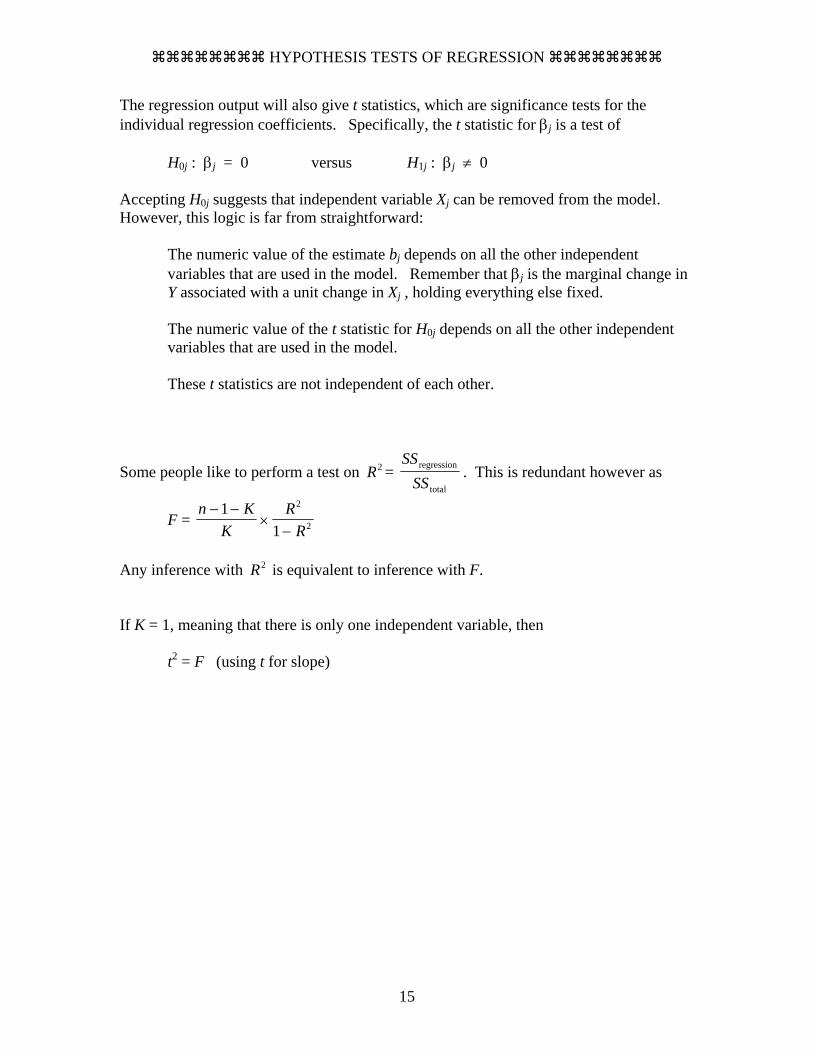
The regression output will also give t statistics, which are significance tests for the individual regression coefficients. Specifically, the t statistic for βj is a test of

H0j : βj = 0 versus H1j : βj ≠ 0

Some people like to perform a test on R2 = SS

SSregression

total. This is redundant however as

F = n K

KR

R− −

×−

11

2

2

Any inference with R2 is equivalent to inference with F. If K = 1, meaning that there is only one independent variable, then

t2 = F (using t for slope)

Accepting H0j suggests that independent variable Xj can be removed from the model. However, this logic is far from straightforward:

The numeric value of the estimate bj depends on all the other independent variables that are used in the model. Remember that βj is the marginal change in Y associated with a unit change in Xj , holding everything else fixed. The numeric value of the t statistic for H0j depends on all the other independent variables that are used in the model. These t statistics are not independent of each other.


16

There are occasions in which we want confidence intervals for the regression coefficients. The 1 - α confidence interval for βj is

bj ± tα/2;n-1-K SE(bj) The standard error SE(bj) requires computer computation, as it involves the inversion of a K-by-K matrix. The value is printed on most computer output. The confidence intervals for β1, β2, …, βK have problems similar to those of the tests.

The confidence intervals for β1, β2, …, βK are not statistically independent.

There is also the issue of predicting for a new Y. This is easily done in Minitab, but you have to supply the new values for the X’s. The resulting interval is called a prediction interval (not a confidence interval), as you are predicting the value of an unobserved random variable. In simple regression (one X), there is a routine formula. Given

n data points (x1, y1), …, (xn, yn) model Yi = β0 + β1 xi + εi

fitted line Y = b0 + b1 x standard error of regression sε a new value xnew for which you’d like a prediction

then the 1 - α prediction for Ynew is

b0 + b1 xnew ± tα/2;n-2 sε 1 12

+ +−

nx x

Snew

xx

b g

The confidence interval for βj depends on all the other independent variables that are used in the model. Remember that βj is the marginal change in Y associated with a unit change in Xj , holding everything else fixed.


17

Aside: You will sometimes see the interval

b0 + b1 xnew ± tα/2;n-2 sε 1

2

nx x

Snew

xx

+−b g

but this is a confidence interval for the parameter combination β0 + β1 xnew . This is a very confusing (and nearly useless) idea, so it should be avoided.

There is a similar technology for general regression (K ≥ 2), but the formulas involve matrix inversion, so we give this to our computer program. In the general regression with K independent variables, you need to specify values for each independent variable to make the prediction. This prediction will be centered around

b0 + b1 Xnew,1 + b2 Xnew,2 + … + bK Xnew,K The computer program will list the prediction interval, and it will be centered around this value. If you use a 95% prediction interval, then the probability is 0.95 that Ynew will fall in the interval.

The computer program will also give a confidence interval. This is merely a confidence interval for the parameter combination

β0 + β1 Xnew,1 + β2 Xnew,2 + … + βK Xnew,K This is not helpful.

Finally, you should be aware that all these inferential steps are correct only at the initial level of work on the first regression run. Generally you will make decisions as to whether to perform transformations, possibly delete high leverage points, and remove predictors from the model. Every step has its own probability of Type I error and Type II error. The probabilities of these Type I errors and Type II errors are complicated and are not completely understood. Thus the inferences that you will eventually make can only be regarded as approximate.

AN EXAMPLE OF VARIABLE SELECTION

18

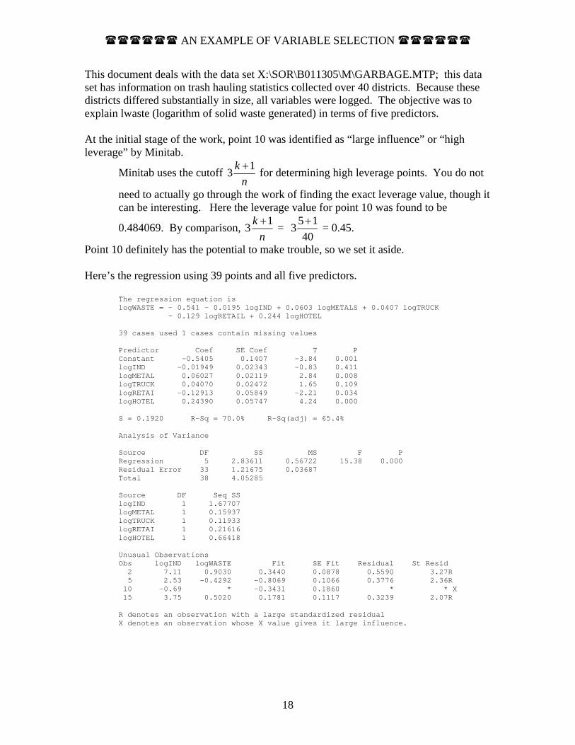
This document deals with the data set X:\SOR\B011305\M\GARBAGE.MTP; this data set has information on trash hauling statistics collected over 40 districts. Because these districts differed substantially in size, all variables were logged. The objective was to explain lwaste (logarithm of solid waste generated) in terms of five predictors. At the initial stage of the work, point 10 was identified as “large influence” or “high leverage” by Minitab.

Minitab uses the cutoff 13 kn+ for determining high leverage points. You do not

need to actually go through the work of finding the exact leverage value, though it can be interesting. Here the leverage value for point 10 was found to be

0.484069. By comparison, 13 kn+ = 5 13

40+ = 0.45.

Point 10 definitely has the potential to make trouble, so we set it aside. Here’s the regression using 39 points and all five predictors.

The regression equation is logWASTE = - 0.541 - 0.0195 logIND + 0.0603 logMETALS + 0.0407 logTRUCK - 0.129 logRETAIL + 0.244 logHOTEL 39 cases used 1 cases contain missing values Predictor Coef SE Coef T P Constant -0.5405 0.1407 -3.84 0.001 logIND -0.01949 0.02343 -0.83 0.411 logMETAL 0.06027 0.02119 2.84 0.008 logTRUCK 0.04070 0.02472 1.65 0.109 logRETAI -0.12913 0.05849 -2.21 0.034 logHOTEL 0.24390 0.05747 4.24 0.000 S = 0.1920 R-Sq = 70.0% R-Sq(adj) = 65.4% Analysis of Variance Source DF SS MS F P Regression 5 2.83611 0.56722 15.38 0.000 Residual Error 33 1.21675 0.03687 Total 38 4.05285 Source DF Seq SS logIND 1 1.67707 logMETAL 1 0.15937 logTRUCK 1 0.11933 logRETAI 1 0.21616 logHOTEL 1 0.66418 Unusual Observations Obs logIND logWASTE Fit SE Fit Residual St Resid 2 7.11 0.9030 0.3440 0.0878 0.5590 3.27R 5 2.53 -0.4292 -0.8069 0.1066 0.3776 2.36R 10 -0.69 * -0.3431 0.1860 * * X 15 3.75 0.5020 0.1781 0.1117 0.3239 2.07R R denotes an observation with a large standardized residual X denotes an observation whose X value gives it large influence.


19

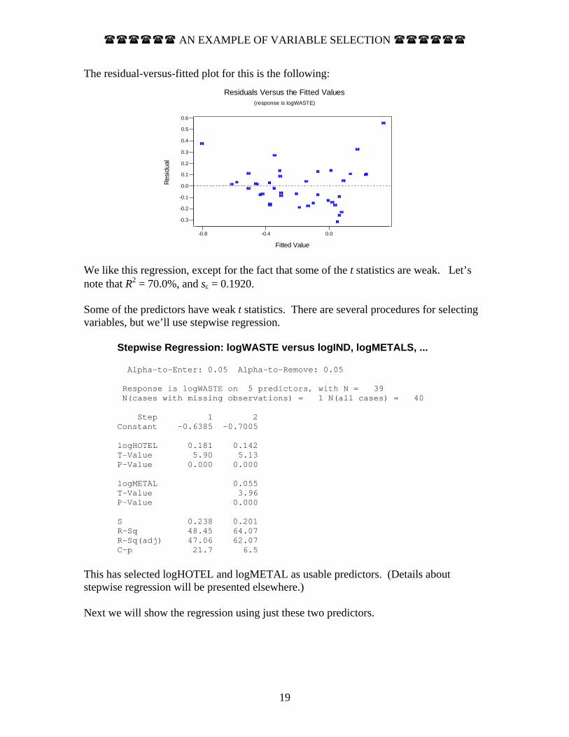
The residual-versus-fitted plot for this is the following:

0.0-0.4-0.8

0.6

0.5

0.4

0.3

0.2

0.1

0.0

-0.1

-0.2

-0.3

Fitted Value

Resi

dual

Residuals Versus the Fitted Values(response is logWASTE)

We like this regression, except for the fact that some of the t statistics are weak. Let’s note that R2 = 70.0%, and sε = 0.1920. Some of the predictors have weak t statistics. There are several procedures for selecting variables, but we’ll use stepwise regression.

Stepwise Regression: logWASTE versus logIND, logMETALS, ... Alpha-to-Enter: 0.05 Alpha-to-Remove: 0.05 Response is logWASTE on 5 predictors, with N = 39 N(cases with missing observations) = 1 N(all cases) = 40 Step 1 2 Constant -0.6385 -0.7005 logHOTEL 0.181 0.142 T-Value 5.90 5.13 P-Value 0.000 0.000 logMETAL 0.055 T-Value 3.96 P-Value 0.000 S 0.238 0.201 R-Sq 48.45 64.07 R-Sq(adj) 47.06 62.07 C-p 21.7 6.5

This has selected logHOTEL and logMETAL as usable predictors. (Details about stepwise regression will be presented elsewhere.) Next we will show the regression using just these two predictors.


20

The regression equation is logWASTE = - 0.700 + 0.0554 logMETALS + 0.142 logHOTEL 39 cases used 1 cases contain missing values Predictor Coef SE Coef T P Constant -0.70049 0.07410 -9.45 0.000 logMETAL 0.05545 0.01402 3.96 0.000 logHOTEL 0.14211 0.02772 5.13 0.000 S = 0.2011 R-Sq = 64.1% R-Sq(adj) = 62.1% Analysis of Variance Source DF SS MS F P Regression 2 2.5967 1.2983 32.10 0.000 Residual Error 36 1.4562 0.0404 Total 38 4.0529 Source DF Seq SS logMETAL 1 1.5335 logHOTEL 1 1.0632 Unusual Observations Obs logMETAL logWASTE Fit SE Fit Residual St Resid 2 6.58 0.9030 0.3590 0.0755 0.5440 2.92R 15 1.50 0.5020 -0.0317 0.0633 0.5337 2.80R 20 4.84 -0.4020 -0.5306 0.1067 0.1286 0.75 X R denotes an observation with a large standardized residual X denotes an observation whose X value gives it large influence.

We see that R2 has dropped, but only to 64.1%. We’re happy to tolerate this drop in R2 to reduce the problem to just two predictors. We see that Minitab has found another large influence point, point 20, but we’re going to react only at the beginning of the work to such messages. The residual versus fitted plot here looks similar to the original. Now that we’re down to only two predictors, maybe point 10 is not troublesome any more. Let’s restore point 10 and see what happens:

The regression equation is logWASTE = - 0.643 + 0.0508 logMETALS + 0.129 logHOTEL Predictor Coef SE Coef T P Constant -0.64349 0.07469 -8.62 0.000 logMETAL 0.05078 0.01476 3.44 0.001 logHOTEL 0.12936 0.02893 4.47 0.000 S = 0.2139 R-Sq = 58.3% R-Sq(adj) = 56.0% Analysis of Variance Source DF SS MS F P Regression 2 2.3611 1.1805 25.81 0.000 Residual Error 37 1.6921 0.0457 Total 39 4.0532


21

Source DF Seq SS logMETAL 1 1.4469 logHOTEL 1 0.9142

Unusual Observations Obs logMETAL logWASTE Fit SE Fit Residual St Resid 2 6.58 0.9030 0.3230 0.0787 0.5800 2.92R 10 -0.69 -0.1672 -0.6262 0.0700 0.4590 2.27R 15 1.50 0.5020 -0.0343 0.0673 0.5363 2.64R 20 4.84 -0.4020 -0.4874 0.1118 0.0854 0.47 X R denotes an observation with a large standardized residual X denotes an observation whose X value gives it large influence.

Point 10 is no longer a high leverage point. You might note that we’ve paid a penalty in R2, a drop from 64.1% to 58.3%, just for putting in this one point. You might look back at the original data. Point 10 is really unusual. Should we react to the fact that point 20 is now identified as having high leverage? Probably not, as the process of editing out points could go on indefinitely. Here is the residual versus fitted plot, with the interesting points marked:

0.40.20.0-0.2-0.4-0.6

0.6

0.5

0.4

0.3

0.2

0.1

0.0

-0.1

-0.2

-0.3

Fitted Value

Resi

dual

Residuals Versus the Fitted Values(response is logWASTE)

20

1015 2

VARIABLE SELECTION ON THE CONDOMINIUM UNITS (reprise)

22

This uses a data set involving prices of condominium units within a Florida development. The data set is taken from Mendenhall and Sincich (the original source has n = 209, and a previous document analyzed a subset of 61). These data are on the Stern network in file X:\SOR\B011305\M\CONDO209.MTP. The variables are

PRICE = selling price of condo unit FLOOR = floor (1 to 8) DELEV = distance from elevator (units unclear; could be yards) VIEW = 1 if view of ocean, 0 otherwise END = 1 if end unit, 0 otherwise FURN = 1 if furnished, 0 otherwise

The objective here will be to relate the obvious dependent variable PRICE to the other variables. The variables VIEW, END, and FURN are called dummy (or indicator) variables because they take only two values. The regression model is

PRICEi = β0 + βFLOOR FLOORi + βDELEV DELEVi + βVIEW VIEWi

+ βEND ENDi + βFURN FURNi + εi

where i = 1, 2, 3, ..., n (Here n = 209.) Note that the coefficients of dummy variables have an immediate and obvious interpretation:

βVIEW represents the added value of an ocean view βEND represents the added value of an end unit βFURN represents the added value of furniture

Suppose that you submit this to Minitab. What follows will be either commentary or output from the program. The commentary will be preceded and followed by ≈≈≈. Variable N Mean Median TrMean StDev SE Mean Min Max Q1 Q3 Price 209 20129 19500 19954 3389 234 13000 30600 17500 21000 Floor 209 4.488 4.000 4.487 2.275 0.157 1.000 8.000 3.000 6.000 DElev 209 7.804 9.000 7.788 4.605 0.319 1.000 15.000 3.500 12.000 View 209 0.5167 1.0000 0.5185 0.5009 0.0346 0.0000 1.0000 0.0000 1.0000 End 209 0.0335 0.0000 0.0000 0.1804 0.0125 0.0000 1.0000 0.0000 0.0000 Furn 209 0.3445 0.0000 0.3280 0.4763 0.0329 0.0000 1.0000 0.0000 1.0000

≈≈≈≈≈≈≈≈≈≈≈≈≈≈≈≈≈≈≈≈≈≈≈≈≈≈≈≈≈≈≈≈≈≈≈≈≈≈≈≈≈≈≈≈≈≈≈≈≈≈≈≈≈≈≈≈≈≈≈≈≈≈≈≈≈ The above is the result of Stat ⇒ Basic Statistics ⇒ Display descriptive Statistics in Minitab, with the results rearranged. Apparently these are not very expensive condo units. The average price was around $20,000. The fact that the mean of VIEW was 0.5167 indicates that about half the units had ocean views. ≈≈≈≈≈≈≈≈≈≈≈≈≈≈≈≈≈≈≈≈≈≈≈≈≈≈≈≈≈≈≈≈≈≈≈≈≈≈≈≈≈≈≈≈≈≈≈≈≈≈≈≈≈≈≈≈≈≈≈≈≈≈≈≈≈


23

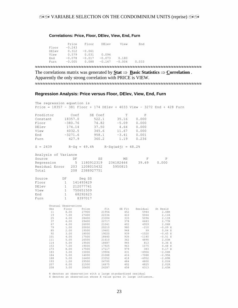
Correlations: Price, Floor, DElev, View, End, Furn Price Floor DElev View End Floor -0.243 DElev 0.312 -0.061 View 0.579 0.031 0.094 End -0.078 -0.017 -0.073 0.180 Furn -0.005 0.088 -0.147 -0.004 0.033

≈≈≈≈≈≈≈≈≈≈≈≈≈≈≈≈≈≈≈≈≈≈≈≈≈≈≈≈≈≈≈≈≈≈≈≈≈≈≈≈≈≈≈≈≈≈≈≈≈≈≈≈≈≈≈≈≈≈≈≈≈≈≈≈≈ The correlations matrix was generated by Stat ⇒ Basic Statistics ⇒ Correlation . Apparently the only strong correlation with PRICE is VIEW. ≈≈≈≈≈≈≈≈≈≈≈≈≈≈≈≈≈≈≈≈≈≈≈≈≈≈≈≈≈≈≈≈≈≈≈≈≈≈≈≈≈≈≈≈≈≈≈≈≈≈≈≈≈≈≈≈≈≈≈≈≈≈≈≈≈ Regression Analysis: Price versus Floor, DElev, View, End, Furn The regression equation is Price = 18357 - 381 Floor + 174 DElev + 4033 View - 3272 End + 428 Furn Predictor Coef SE Coef T P Constant 18357.0 522.1 35.16 0.000 Floor -380.76 74.82 -5.09 0.000 DElev 174.14 37.50 4.64 0.000 View 4032.5 345.6 11.67 0.000 End -3271.6 958.1 -3.41 0.001 Furn 427.9 360.2 1.19 0.236 S = 2439 R-Sq = 49.4% R-Sq(adj) = 48.2% Analysis of Variance Source DF SS MS F P Regression 5 1180912319 236182464 39.69 0.000 Residual Error 203 1208015432 5950815 Total 208 2388927751 Source DF Seq SS Floor 1 141493429 DElev 1 212077741 View 1 750651509 End 1 68292623 Furn 1 8397017

Unusual Observations Obs Floor Price Fit SE Fit Residual St Resid 11 8.00 27900 21956 452 5944 2.48R 19 7.00 27400 22336 410 5064 2.11R 25 4.00 28400 23304 333 5096 2.11R 37 6.00 29400 22717 378 6683 2.77R 67 4.00 26000 21041 402 4959 2.06R 79 1.00 20000 20210 980 -210 -0.09 X 85 2.00 19500 19401 948 99 0.04 X 92 3.00 18000 19020 939 -1020 -0.45 X 101 4.00 17500 18640 935 -1140 -0.51 X 111 5.00 26500 21610 362 4890 2.03R 114 5.00 19500 18687 945 813 0.36 X 153 7.00 19000 17925 963 1075 0.48 X 173 8.00 17500 17117 979 383 0.17 X 183 3.00 15000 19906 431 -4906 -2.04R 184 5.00 14000 21088 416 -7088 -2.95R 188 5.00 16400 23352 418 -6952 -2.89R 193 1.00 29500 24700 484 4800 2.01R 207 6.00 21500 16675 402 4825 2.01R 208 3.00 30600 24287 458 6313 2.63R R denotes an observation with a large standardized residual X denotes an observation whose X value gives it large influence.


24

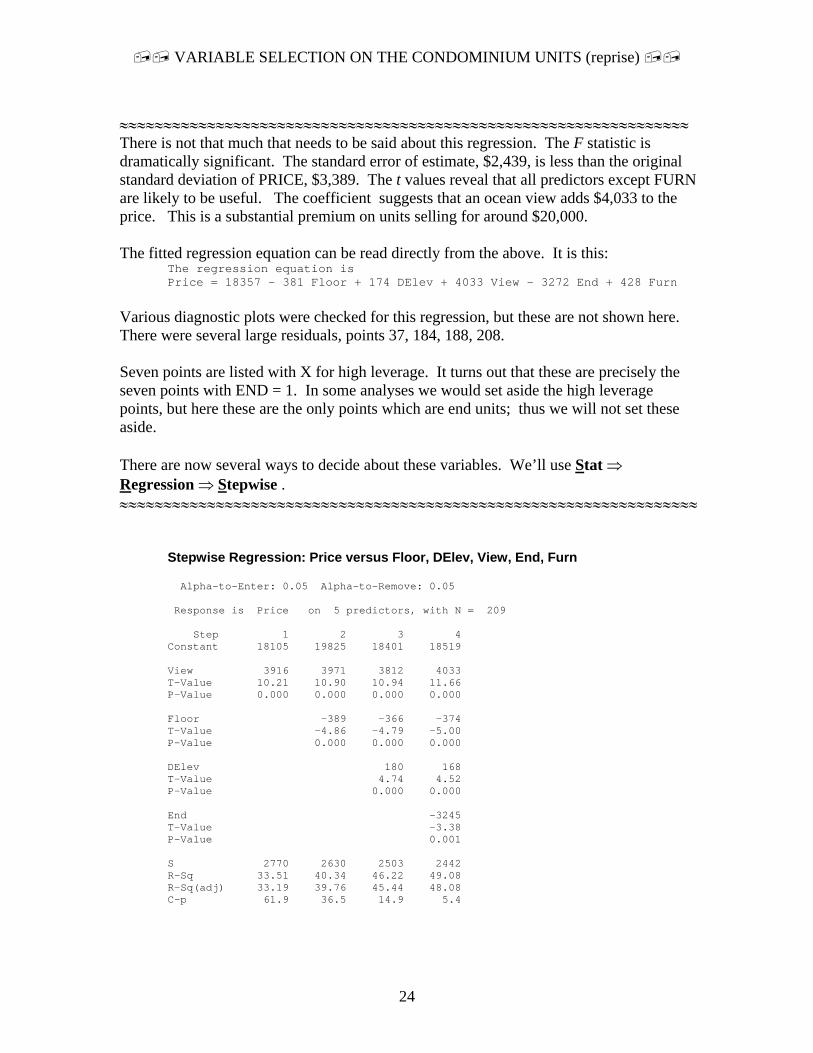
≈≈≈≈≈≈≈≈≈≈≈≈≈≈≈≈≈≈≈≈≈≈≈≈≈≈≈≈≈≈≈≈≈≈≈≈≈≈≈≈≈≈≈≈≈≈≈≈≈≈≈≈≈≈≈≈≈≈≈≈≈≈≈≈≈ There is not that much that needs to be said about this regression. The F statistic is dramatically significant. The standard error of estimate, $2,439, is less than the original standard deviation of PRICE, $3,389. The t values reveal that all predictors except FURN are likely to be useful. The coefficient suggests that an ocean view adds $4,033 to the price. This is a substantial premium on units selling for around $20,000. The fitted regression equation can be read directly from the above. It is this:

The regression equation is Price = 18357 - 381 Floor + 174 DElev + 4033 View - 3272 End + 428 Furn

Various diagnostic plots were checked for this regression, but these are not shown here. There were several large residuals, points 37, 184, 188, 208. Seven points are listed with X for high leverage. It turns out that these are precisely the seven points with END = 1. In some analyses we would set aside the high leverage points, but here these are the only points which are end units; thus we will not set these aside. There are now several ways to decide about these variables. We’ll use Stat ⇒ Regression ⇒ Stepwise . ≈≈≈≈≈≈≈≈≈≈≈≈≈≈≈≈≈≈≈≈≈≈≈≈≈≈≈≈≈≈≈≈≈≈≈≈≈≈≈≈≈≈≈≈≈≈≈≈≈≈≈≈≈≈≈≈≈≈≈≈≈≈≈≈≈≈

Stepwise Regression: Price versus Floor, DElev, View, End, Furn Alpha-to-Enter: 0.05 Alpha-to-Remove: 0.05 Response is Price on 5 predictors, with N = 209 Step 1 2 3 4 Constant 18105 19825 18401 18519 View 3916 3971 3812 4033 T-Value 10.21 10.90 10.94 11.66 P-Value 0.000 0.000 0.000 0.000 Floor -389 -366 -374 T-Value -4.86 -4.79 -5.00 P-Value 0.000 0.000 0.000 DElev 180 168 T-Value 4.74 4.52 P-Value 0.000 0.000 End -3245 T-Value -3.38 P-Value 0.001 S 2770 2630 2503 2442 R-Sq 33.51 40.34 46.22 49.08 R-Sq(adj) 33.19 39.76 45.44 48.08 C-p 61.9 36.5 14.9 5.4


25

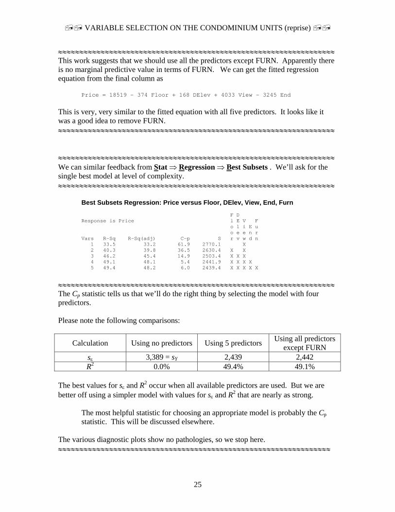
≈≈≈≈≈≈≈≈≈≈≈≈≈≈≈≈≈≈≈≈≈≈≈≈≈≈≈≈≈≈≈≈≈≈≈≈≈≈≈≈≈≈≈≈≈≈≈≈≈≈≈≈≈≈≈≈≈≈≈≈≈≈≈≈≈ This work suggests that we should use all the predictors except FURN. Apparently there is no marginal predictive value in terms of FURN. We can get the fitted regression equation from the final column as

Price = 18519 - 374 Floor + 168 DElev + 4033 View - 3245 End

This is very, very similar to the fitted equation with all five predictors. It looks like it was a good idea to remove FURN. ≈≈≈≈≈≈≈≈≈≈≈≈≈≈≈≈≈≈≈≈≈≈≈≈≈≈≈≈≈≈≈≈≈≈≈≈≈≈≈≈≈≈≈≈≈≈≈≈≈≈≈≈≈≈≈≈≈≈≈≈≈≈≈≈≈ ≈≈≈≈≈≈≈≈≈≈≈≈≈≈≈≈≈≈≈≈≈≈≈≈≈≈≈≈≈≈≈≈≈≈≈≈≈≈≈≈≈≈≈≈≈≈≈≈≈≈≈≈≈≈≈≈≈≈≈≈≈≈≈≈≈ We can similar feedback from Stat ⇒ Regression ⇒ Best Subsets . We’ll ask for the single best model at level of complexity. ≈≈≈≈≈≈≈≈≈≈≈≈≈≈≈≈≈≈≈≈≈≈≈≈≈≈≈≈≈≈≈≈≈≈≈≈≈≈≈≈≈≈≈≈≈≈≈≈≈≈≈≈≈≈≈≈≈≈≈≈≈≈≈≈≈

Best Subsets Regression: Price versus Floor, DElev, View, End, Furn F D Response is Price l E V F o l i E u o e e n r Vars R-Sq R-Sq(adj) C-p S r v w d n 1 33.5 33.2 61.9 2770.1 X 2 40.3 39.8 36.5 2630.4 X X 3 46.2 45.4 14.9 2503.4 X X X 4 49.1 48.1 5.4 2441.9 X X X X 5 49.4 48.2 6.0 2439.4 X X X X X

≈≈≈≈≈≈≈≈≈≈≈≈≈≈≈≈≈≈≈≈≈≈≈≈≈≈≈≈≈≈≈≈≈≈≈≈≈≈≈≈≈≈≈≈≈≈≈≈≈≈≈≈≈≈≈≈≈≈≈≈≈≈≈≈≈ The Cp statistic tells us that we’ll do the right thing by selecting the model with four predictors. Please note the following comparisons:

Calculation Using no predictors Using 5 predictors Using all predictors except FURN

sε 3,389 = sY 2,439 2,442 R2 0.0% 49.4% 49.1%

The best values for sε and R2 occur when all available predictors are used. But we are better off using a simpler model with values for sε and R2 that are nearly as strong.

The most helpful statistic for choosing an appropriate model is probably the Cp statistic. This will be discussed elsewhere.

The various diagnostic plots show no pathologies, so we stop here. ≈≈≈≈≈≈≈≈≈≈≈≈≈≈≈≈≈≈≈≈≈≈≈≈≈≈≈≈≈≈≈≈≈≈≈≈≈≈≈≈≈≈≈≈≈≈≈≈≈≈≈≈≈≈≈≈≈≈≈≈≈≈≈≈


26

There is one additional pathology with these data. This shows up on the plot of the residuals versus the predictors. In particular, the residuals versus DELEV is disconcerting:

151050

5000

0

-5000

DElev

Res

idua

l

Residuals Versus DElev(response is Price)

This suggests curvature in the relationship with DELEV. Suppose that we create variable D2 = DELEV × DELEV. The regression for this situation is the following:

Regression Analysis: Price versus Floor, DElev, View, End, Furn, D2 The regression equation is Price = 20398 - 373 Floor - 670 DElev + 3869 View - 2136 End + 488 Furn + 55.3 D2 Predictor Coef SE Coef T P Constant 20398.1 625.6 32.61 0.000 Floor -372.87 70.36 -5.30 0.000 DElev -670.0 164.3 -4.08 0.000 View 3869.0 326.4 11.85 0.000 End -2135.6 926.3 -2.31 0.022 Furn 488.2 338.9 1.44 0.151 D2 55.32 10.51 5.26 0.000 S = 2293 R-Sq = 55.5% R-Sq(adj) = 54.2% Analysis of Variance Source DF SS MS F P Regression 6 1326515068 221085845 42.04 0.000 Residual Error 202 1062412683 5259469 Total 208 2388927751

EXAMPLE WITH BRUTAL COLLINEARITY

27

The data set used in this illustration is given in Berenson and Levine, 4th edition. The values describe quantities related to the budges at a number of large universities.

SCHOOL VOLUMES VOLADDED SERIALS BUDGET Yale 8236.7 174.7 57.4 19850.4 Columbia 5551.7 121.7 63.4 18031.2 Minnesota 4286.4 116.5 44.6 14956.7 Indiana 3787.0 118.3 32.6 11906.5 Penn 3376.9 106.2 30.5 12468.6 NYU 2932.1 74.7 29.8 12801.8 Duke 3510.6 92.1 35.7 11074.0 Florida 2539.4 78.9 29.5 9875.5 LSU 2210.8 65.3 22.8 8008.8 MIT 2029.5 81.9 21.1 8719.2 West_Ont 1868.9 62.0 19.0 7130.9 Wash_StL 2069.7 43.3 16.5 8103.6 Emory 1951.1 66.9 18.0 8340.1 S_Carolina 2175.8 65.9 18.9 5788.8 Irvine 1239.1 61.0 15.9 9089.0 Nebraska 1833.6 62.8 23.8 5941.3 Ga_Tech 1468.6 49.9 28.6 4308.4 McMaster 1218.1 47.5 18.2 6069.8 Riverside 1250.4 47.2 13.7 6303.2 Saskatchwan 1254.0 47.9 10.1 5241.2 Oklahoma_St 1420.6 30.3 10.4 4699.8

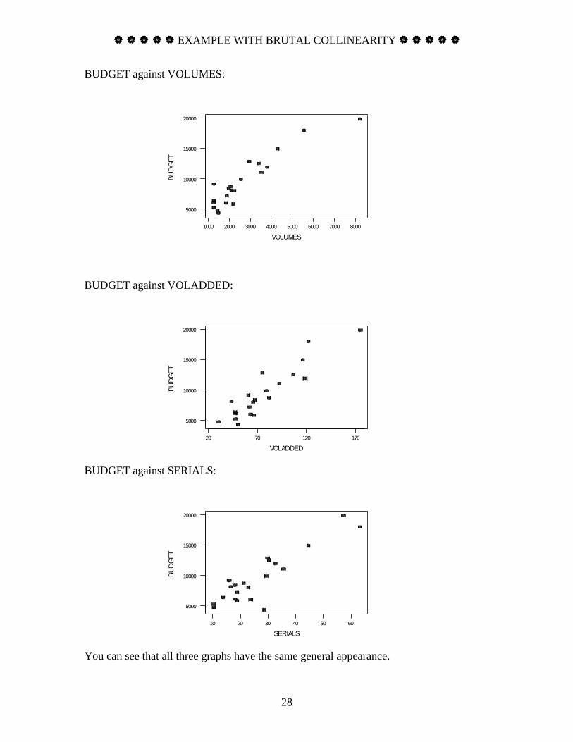
The columns are SCHOOL = school name VOLUMES = library volume (in 1000s) VOLADDED = volumes added in last year (in 1000s) SERIALS = current serials (in 1000s) BUDGET = expenditures for materials and salaries (in $1000s). Find the regression of BUDGET on (VOLUMES, VOLADDED, SERIALS). Give the F statistic. Give also the t statistics for the coefficients. What is the conflicting nature of your findings? Why does it happen? SOLUTION: It’s helpful, before beginning the hard work, to examine some plots. Here are plots of the dependent variable against each of the three independent variables.


28

BUDGET against VOLUMES:

80007000600050004000300020001000

20000

15000

10000

5000

VOLUMES

BUD

GET

BUDGET against VOLADDED:

1701207020

20000

15000

10000

5000

VOLADDED

BUD

GET

BUDGET against SERIALS:

605040302010

20000

15000

10000

5000

SERIALS

BUD

GET

You can see that all three graphs have the same general appearance.


29

You might consider the possibility of replacing each variable by its logarithm. In this case, the decision is marginal. Moreover, the managers might have wanted a cost analysis and resisted the taking of logarithms. Let’s get now the regression of BUDGET on all three predictors. We will have some interest in the VIF (variance inflation factor) numbers, so we will request these.

Regression Analysis The regression equation is BUDGET = 1567 + 0.854 VOLUMES + 44.4 VOLADDED + 82.3 SERIALS Predictor Coef SE Coef T P VIF Constant 1567 1074 1.46 0.163 VOLUMES 0.8544 0.7265 1.18 0.256 12.9 VOLADDED 44.37 31.45 1.41 0.176 9.7 SERIALS 82.28 58.92 1.40 0.181 5.8 S = 1551 R-Sq = 88.8% R-Sq(adj) = 86.9% Analysis of Variance Source DF SS MS F P Regression 3 325360308 108453436 45.09 0.000 Error 17 40887143 2405126 Total 20 366247451 Source DF Seq SS VOLUMES 1 314544162 VOLADDED 1 6125101 SERIALS 1 4691045 Unusual Observations Obs VOLUMES BUDGET Fit StDev Fit Residual St Resid 1 8237 19850 21079 1351 -1229 -1.61 X 2 5552 18031 16927 1187 1104 1.11 X 17 1469 4308 7389 794 -3081 -2.31R R denotes an observation with a large standardized residual X denotes an observation whose X value gives it large influence.

The overall F statistic is 45.09, on (3, 17) degrees of freedom. This is highly significant (P=0.000 to the precision given). The individual t statistics are 1.18 for VOLUMES 1.41 for VOLADDED 1.40 for SERIALS and none are significant. The reason that happens can be seen in the graphs. The relationship of BUDGET to each of the individual independent variables (predictors) is approximately the same. Moreover, the independent variables are strongly related to each other, as seen in the somewhat high VIF values. Thus, BUDGET is definitely strongly related to the predictors (as decided by the F statistic), but none of the predictors contribute anything to the relationship which cannot be attributed to one of the other predictors.


30

By the way, you might ask what would happen if you did not use all three predictor variables. Here is a short summary:

Estimated Coefficients Variables in model

R2 sε Constant VOLUMES (V)

VOLADDED (VA)

SERIALS (S)

none 0.0% 4,279.30 9,462.32 V 85.9% 1,649.61 3,266.56 2.315 VA 84.4% 1,733.40 664.57 144.4 S 80.2% 1,955.57 2,244.98 207.4V,VA 87.6% 1,591.26 1,967.06 1.369 49.8 V, S 87.5% 1,592.98 2,656.90 1.620 92.6 VA,S 87.9% 1,567.25 792.15 72.0 117.5V,VA,S 88.8% 1,550.85 1,566.57 0.854 44.4 82.3

☯ ☯ ☯ ☯ ☯ STRATEGY FOR VARIABLE SELECTION ☯ ☯ ☯ ☯ ☯

31

This document gives a plausible approach to multiple regression. The advice given here works as well for simple regression, but not all the steps are involved. The advice given here cannot be universally guaranteed. Yes, it works well for most situations, but multiple regression is just too complicated a task to allow for a pure cookbook approach. Experience helps. It will be assumed that the input data can be structured as follows:

x11, x12, x13, …, x1K, Y1 x21, x22, x23, …, x2K, Y2 x31, x32, x33, …, x3K, Y3 . . . . . . . . . . xn1, xn2, xn3, …, xnK, Yn

We will designate the variable Y as the dependent variable. The second subscripts of the x’s identify the independent variables, and we can name these variables as X1, X2, …, XK . In accordance with the spreadsheet layout, we will use rows to refer to data points and columns to refer to variables. The model will be

Yi = β0 + β1 xi1 + β2 xi2 + β3 xi3 + … + βK xiK + εi The noise terms ε1, ε2, ..., εn are random and unobserved. Moreover, we assume that these ε’s are statistically independent, each with mean 0 and (unknown) standard deviation σε. Multiple regressions can be done for many reasons, but our objectives will be the following:

Obtain estimates for the β’s. Based on statistical tests, decide if perhaps some of the β’s might really be zero. If so, the regression model can be simplified by removing some of the independent variables. Obtain an estimate for σε , the standard deviation of the noise terms. Check statistical measures such as the F statistic, R2 , and the standard error of estimate (the estimate of σε) to assure that the regression was worth doing.


32

Examine secondary information (such as scatterplots) to assess whether the assumptions behind the model are reasonable. If the situation calls for making predictions, then those predictions should be made, along with prediction intervals.

Here now are a number of steps. This procedure usually works. 0. Do you have missing data values? If not, proceed to step 1. Data points (rows) in which the dependent variable is missing must be discarded; you have no choice about this. The difficulty now is to eliminate rows or columns, or both, to reduce the number of missing data values. Variables (columns) with an excessive number of missing values (more than 10%, say) should be discarded. Data points (rows) with several missing values should be discarded. This entire process is subjective. Some people are willing to work with a set of data in which there are just a small number of missing values. Others will insist that the data set be complete. At this point, you should also check the basic integrity of your data. Do the maximum and minimum values for each variable make sense? If you are willing to work with data containing missing values, please be sensitive to the fact that the apparent sample size n will change as you eliminate variables. This could be absolutely maddening to the users of your report. 1. If K, the number of independent variables is moderate, say K ≤ 10, then skip this step. If K is very large, say K ≥ 30, you would find it helpful to eliminate immediately some of the independent variables. A simple procedure examines the Pearson correlation matrix and removes from consideration one variable from each pair producing an extreme correlation (say above 0.99 or below -0.99). Subjective choices will have to be made. If K is between 10 and 30 (say), then use your judgment. In the steps that follow, the symbol K refers to the number of independent variables remaining after step 1, not the original number. 2. Make a simple stem-and-leaf plot (or boxplot or histogram) of the dependent variable Y and of each of the K independent variables. If any plots show excessive skewness, consider a transformation. Excessive skewness usually shows up as a few extremely large values (but no very low values). This problem can almost always be cured by replacing the variable with its logarithm. If the variable, say X3, has some zeroes or negative values, use log(X3 + c) where c is sufficiently large to make all values of xi3 + c > 0.


33

3. Perform the regression of Y on all the independent variables under consideration. Note the value of R2 and the value of the standard error of estimate.

If the program refuses to do the regression, perhaps giving you a message like “singular matrix” or “unable to perform matrix inversion” or “excessive collinearity” or “bad condition number,” you must resort to a method which forces you to reduce the number of independent variables. One method that works is to eliminate independent variables which show very high Pearson correlations (over 0.99 or under -0.99) with other variables; there are some subjective choices to be made. A second technique is that of stepwise regression, which is available with many computer packages.

If the computer package provides leverage values, data rows with large leverage values should be checked for correctness. Points with large leverage values may be destructive to the regression. If any of the n data points has a very large leverage value, say greater

than 3 1Kn+ , then you should consider removal of that point. The program Minitab will

automatically marked data points with leverage greater than 3 1Kn+ , so you need not

have the leverage values produced as numbers. If you remove one or more points based on leverage, return to the start of step 3. (The leverage values need not be checked again until step 6.)

You should be very conservative about removing points from a regression based on high leverage. If you remove data points in step 3 because of high leverage issues, there is a very large chance that you will end up restoring those points in step 6. Points need to be really weird to justify their removal.

4. Examine all the t statistics (except the t for the constant or intercept). There is one such statistic for each estimated coefficient. If any p-value exceeds 0.05, then you may be carrying too many predictor variables. There are many strategies for removing extra predictors, but you might want to depend on the reliable methods of stepwise regression and best subsets regression. (These are discussed elsewhere in this document.) If all the p-values statistics are at or below 0.05, then go to step 5.

[Ignore this paragraph the first time you do step 3.] If you are repeating step 3 after removing some of the independent variables based on step 4, make sure that your R2 value is not appreciably worse (smaller) and that your standard error of estimate is not appreciably worse (larger). If either or both of these looks worse, then you have removed too many independent variables. Put some of them back in the model and return to the start of step 3.


34

You might also have a collinearity problem. The removal rule listed here would cause you to remove too many variables. You can make a good decision by using stepwise regression or best subsets. With best subsets, select the simplest model for which Cp is approximately equal to p. The best subsets and stepwise methods frequently agree perfectly. In problems with a singular matrix (as mentioned in step 3), you might not be able to use the best subsets method. After you have removed some variables, the value of K is reduced. Return to step 3. 5. You have found a tentative working regression model. It’s necessary to check the assumptions. The most important check is the residual-versus-fitted plot, which is provided with most computer packages. If this plot appears patternless, proceed. If there is a pattern, you’ve got to take action. The most common pattern is that of expanding residuals, and this can be cured by replacing Y by its logarithm. (See the comments on logarithms in step 2.) A more difficult pattern is that of curvature, suggesting that the linear relationship between Y and the x’s is incorrect. Ask for a delay in the project deadline while you seek help! Does the sequencing of the index i = 1, 2, ...., n refer to actual time order? If not, skip this paragraph. Ask for a sequence plot of the residuals; this can reveal problems. Examine the Durbin-Watson statistic. If this statistic is far from its baseline value of 2 (for example, if it is below 1.25), then the problem has large autocorrelation of the noise terms. There are many possible corrections for this problem, but the simplest one is to replace Y and all the independent variables by their differences. For example, Y8 is replaced by Y8 – Y7. Unfortunately, you’ve got to start over from step 1. 6. Did you remove any data points in step 3 based on leverage values? If not, proceed to step 7. If yes, note that you’ve changed the problem considerably since the removal of those points, and you might now be able to return those points to the problem. Thus, you should consider the leverage issue again; many software packages will give you the leverage values for points not presently included in the regression calculation. You can readmit these points to the data set if the leverage values are not severe. This is all quite subjective. Generally, we want to be conservative about throwing points out of the data set and then somewhat cautious about readmitting them. 7. You’re done. At a minimum, the report for the regression should consist of the fitted regression model, the standard errors for the estimated coefficients, the F statistic (with its degrees of freedom), and standard error of estimate, and the standard deviation of Y. If the situation required a prediction, that prediction should be made, along with an interval. You should be aware that the standard error of estimate was obtained after a search procedure (say in best subsets), so it might be unrealistically small.

REF LIST (NOT FOR DISTRIBUTION)

35

Document sources (not part of handout) mregcndo.doc (a very simple variable selection; end up with one predictor) collin2002.doc (notes cp stepwise bestsubsets) Easton.doc shows issues related to indicators, variable selection, predictions hyptestR.doc (including some prediction, caveats about inference after selection) mreggood.doc (not the B version; this is the garbage hauling data; this shows stepwise) mregcondo209.doc (as above, but with bigger n and different answer) mreglibr.doc (an example with brutal collinearity) regmeth.doc (shows a procedure, including variable selection)