Multiple Location Profiling for Users and Relationshipsfrom Social Network and Content

∗

Rui Li†

ruili1@illinois.edu

Shengjie Wang†

wang260@illinois.edu

Kevin Chen-ChuanChang†,∗

kcchang@illinois.edu† Department of Computer Science, University of Illinois at Urbana-Champaign, Urbana, IL, USA

∗ Advanced Digital Sciences Center, Illinois at Singapore, Singapore

ABSTRACT

Users’ locations are important for many applications suchas personalized search and localized content delivery. Inthis paper, we study the problem of profiling Twitter users’locations with their following network and tweets. We pro-pose a multiple location profiling model (MLP), which hasthree key features: 1) it formally models how likely a userfollows another user given their locations and how likely auser tweets a venue given his location, 2) it fundamentallycaptures that a user has multiple locations and his followingrelationships and tweeted venues can be related to any ofhis locations, and some of them are even noisy, and 3) itnovelly utilizes the home locations of some users as partialsupervision. As a result, MLP not only discovers users’ loca-tions accurately and completely, but also “explains” each fol-lowing relationship by revealing users’ true locations in therelationship. Experiments on a large-scale data set demon-strate those advantages. Particularly, 1) for predicting users’home locations, MLP successfully places 62% users and out-performs two state-of-the-art methods by 10% in accuracy,2) for discovering users’ multiple locations, MLP improvesthe baseline methods by 14% in recall, and 3) for explainingfollowing relationships, MLP achieves 57% accuracy.

1. INTRODUCTIONUsers’ locations are important information for many ad-

vanced information services, such as delivering localized news,recommending friends and serving targeted ads.Recently, social network sites, such as Facebook and Twit-

ter, become important platforms for users to connect with

∗This material is based upon work partially supported by NSF Grant

IIS 1018723, the Advanced Digital Science Center of the University ofIllinois at Urbana-Champaign and the Multimodal Information Ac-cess and Synthesis Center at UIUC. Any opinions, findings, and con-clusions or recommendations expressed in this publication are thoseof the author(s) and do not necessarily reflect the views of the fundingagencies.

Location: Los Angeles Education: Uni. of Texas at Austin

Carol

?

Lucy

Austin

Gaga

NY

Mike

LA

Bob

San Diego

Jean

?

Want to go to Honolulu

for Spring vacation!

See Gaga in Hollywood.

Good Morning!

The Following Network Tweets

Carol’s Location Profile: Los Angeles, Austin

Carol follows Lucy: Austin; Austin

Figure 1: Building Location Profiles for Users

friends and share information. For example, Twitter, a so-cial network for users to follow others and publish tweets,now has 140 million active users and generates 340 milliontweets daily. However, for most of users on these sites, theirlocations are missing. For example, on Twitter, only a fewusers (16%) register city level locations (e.g., Los Angeles,CA). Most of them leave nonsensical (e.g., “my home”), gen-eral (e.g., “CA”) or even blank information. Although Twit-ter supports GPS tags in tweets, even fewer users (0.5%) usethis feature due to obvious privacy concerns.

In the literature, many methods [8, 5, 11] have been pro-posed to profile users’ locations in the context of social net-work. Specifically, they focus on profiling a user’s home

location, which is the single ”permanent” resident locationof the user, by exploring her social network (e.g., friendship-s) and content (e.g., tweets). Intuitively, both types of dataprovide valuable signals for profiling users’ locations, as auser is likely to 1) connect to others living close to her, and2) tweet her nearby “venues”.

However, these methods have the same shortcoming –they assume that a user has only a “home location”. Inreality, as illustrated in Fig. 1, a user (e.g., Carol) is relat-ed to multiple locations, such as her home location (e.g.,Los Angeles) and college location (e.g., Austin). She followsfriends from and tweets venues about all of them. E.g., Carolfollows her classmate Lucy in Austin and her co-worker Bobin Los Angeles. Thus, these methods not only profile herlocations incompletely, but also estimate her home locationinaccurately, because signals related to her other locationsare noises for profiling even just her home location.

1603

Permission to make digital or hard copies of all or part of this work forpersonal or classroom use is granted without fee provided that copies arenot made or distributed for profit or commercial advantage and that copiesbear this notice and the full citation on the first page. To copy otherwise, torepublish, to post on servers or to redistribute to lists, requires prior specificpermission and/or a fee. Articles from this volume were invited to presenttheir results at The 38th International Conference on Very Large Data Bases,August 27th - 31st 2012, Istanbul, Turkey.Proceedings of the VLDB Endowment, Vol. 5, No. 11Copyright 2012 VLDB Endowment 2150-8097/12/07... $ 10.00.

In this paper, we aim to build complete “location profiles”for Twitter users with their following network and tweets.We define a user’s (e.g., Carol) location profile as a set oflocations related to her (e.g., Los Angeles, Austin). Itincludes not only her home location (e.g., Los Angeles) butalso her other related locations (e.g., Austin). Further, weclarify that each user related location is 1) a geo scope (e.g.,Los Angeles) instead of a geo point (e.g., the Starbucks on5th Ave.), and 2) a long-term location instead of a tempo-

rally related location (e.g., the places where he is traveling).Thus, a user’s location profile captures her multiple long-term geographic scopes of interests. We emphasize that weonly use users’ following network and tweets, and do notuse GPS tags because they are rarely available as we justmentioned. Thus, we avoid the need for private information(e.g., IP address) and enable third-party services (e.g., re-searchers) to profile users’ locations with Twitter open APIs.In addition, for each relationship (e.g., the following rela-

tionship from Carol to Lucy), we aim to profile users’ specif-ic locations underlying the relationship (e.g., Carol followsLucy as they studied in Austin), because a user has mul-tiple locations of interest and each of her relationships canbe a result of any of her locations. Profiling locations foreach relationship not only helps us to discover users’ loca-tions accurately and completely, but also enables interestingapplications, such as understanding the true geo connectionbetween two users and grouping a user’s friends into geogroups (e.g., Carol is in Lucy’s Austin group).Thus, we propose a multiple location profiling model (MLP)

for users and their relationships. To the best of our knowl-edge, MLP is the first model that 1) discovers users’ multiplelocations and 2) profiles both users and their relationships.Specifically, MLP takes a generative probabilistic approach

and models the joint probability of generating “following”and “tweeting” relationships based on users’ multiple loca-tions. With the joint probability, we estimate users’ loca-tions and locations of relationships as latent variables in theprobability. However, when modeling the joint probability,MLP must deal with the following challenges.

Location-based Generation To connect users’ locationswith observed relationships, MLP needs to formally modelthe probability that a relationship is generated based onusers’ locations. Specifically, it should capture that a userat a specific location 1) follows her friends from differentlocations or tweets different venues, and 2) is likely to followusers living close to her or tweet her nearby venues.We thoroughly investigate the connections between the t-

wo types of relationships and users’ locations on a large-scaleTwitter data and derive a location-based generative model

for each type of relationships. For the “following probabili-ty” based on two user’s locations, we explore the probabilitybased on their distance, and formally model the probabilitiesover distances as a power law distribution. For the “tweetingprobability” based on one user’s location, we view locationsand venues as discrete labels, and formally model the prob-abilities of tweeting different venues at each location as amultinomial distribution over a set of venues.

Mixture of Observations We can not straightforward-ly use observed relationships to build a user’ location pro-file, because of two challenges: 1) the noisy-signal challenge,which means she may follow friends (e.g., Lady Gaga) andtweet venues (e.g., Honolulu) that are not based on her loca-tions, 2) the mixed-signal challenge, which means she follows

friends (e.g., Lucy and Bob) or tweets venues based on hermultiple locations. We introduce two mixtures in MLP todeal with the two challenges.

With respect to the noisy-signal challenge, we model re-lationships as a mixture of “noisy” and “location-based” re-lationships. Specifically, we introduce a random generative

model to model how a noisy relationship is generated ran-domly, besides the location-based generative model intro-duced above. Each relationship is generated by either of thetwo models with a certain probability. Thus, MLP explicit-ly captures noisy relationships, and automatically rules outthem when profiling users’ locations.

With respect to the mixed-signal challenge, we extendthe location-based generative models to generate relation-ships based on users’ multiple locations. Specifically, weview a user’s location profile as a multinomial distributionover a set of locations, and extend the models to generatea location-based relationship in two steps: 1) generate a lo-cation assignment from each related user’s location profile,and 2) generate the relationship based on the assignments.Thus, MLP fundamentally captures that a user has mul-tiple locations. It not only discovers her multiple locationscompletely, but also estimates her home location accurately.Further, MLP reveals the true geo connection in a relation-ship with the location assignments for the relationship.

Partially Available Supervision As we mentioned thatsome users provide their home locations, those locations arethe only observed locations and crucial for accurate profiling.However, they are difficult to use, because we can neitherview them as users’ location profiles, as a profile should con-tain more than a home location, nor use them to generaterelationships because of the mixed-signal challenge.

We incorporate the observed home locations as prior knowl-edge to generate users’ location profiles. Specifically, we as-sume that a user’s location profile is generated via a priordistribution with a hyper parameter, and use the observedlocations to set the hyper parameter for each user. As a re-sult, for a user with an observed location, her derived loca-tion profile has a large probability to generate the observedlocation, and her relationships are likely to be generatedbased on the location as well.

Based on MLP, we profile users and their relationshipsas estimating the latent variables in the joint probability.However, as MLP models the above new aspects and inte-grates discrete (multinomial) and continuous (power low)distributions, it does not allow exact inference. We derivean efficient sampling-based algorithm based on the Gibbssampling framework to estimate the latent variables.

To evaluate MLP, we conduct extensive experiments andcompare MLP with the stare-of-the-art methods [5, 8] on alarge-scale Twitter data containing about 160K users. Theresults show that MLP is effective. Specifically, 1) for pre-dicting users’ home locations, MLP largely improves thebaseline methods by 10% and places 62% users accurately;2) for discovering users’ multiple locations, MLP capturesusers’ multiple locations accurately and completely, and im-proves the baseline methods by 11% and 14% in terms of“precision” and “recall”; 3) for explaining following rela-tionships, MLP achieves 57% accuracy.

The rest of this paper is organized as follows. We reviewthe literature in Sec. 2, formalize our problem in Sec. 3, anddevelop our model in Sec. 4. Finally, we present experimentsin Sec. 5 and conclude our work in Sec. 6.

1604

2. RELATED WORKIn this section, we discuss some related work. In terms

of the problem, our work is related to location prediction.In terms of the technique, our work is related to collectiveclassification and mixture models.

Location Prediction As we focus on profiling users’ lo-cations, our work is related to identifying the geographicalscope of various kinds of online resources, such as pages [10,2], queries [4], tags [17], and photos [9]. However, they pre-dict locations for different types of entities with different re-sources. For example, Amitay et al. [2] explore a web page’scontent to predict its geo scope via heuristically associat-ing extracted location signals (e.g., city names) to locationswith a gazetteer. Our work is different, as we take a prob-abilistic approach to profile users’ locations. Backstrom etal. [4] use a probabilistic model to assign a geographic centerto a query based on its usage. Our probabilistic model isdifferent, as it models generating following relationships andtweeted venues based on users’ locations and assumes thata user has multiple locations.Our work is most related to [8, 5, 11], as they profile

users’ locations as well. Cheng et al. [8] estimate a user’slocation based on his tweets. They identify a set of loca-tion related words (e.g., “houston”) and use these words asfeatures to classify a user to locations. Backstrom et al. [5]estimate a user’s location based on his friends on Facebook.They learn a function which assigns the probability of beingfriends given the distance of two users, and then estimate auser’s location based on the maximum likelihood estimationprinciple. Recently, we propose a generative model to inte-grate both social network and tweets [11]. However, as wediscussed in Sec. 1, as those methods assume a user has onlyone location, they not only profile a user’s locations incom-

pletely, but also estimate his home location inaccurately.

Collective Classification As we aim to assign users ina social network to location labels, our work is related tocollective classification [18], which classifies objects in a net-work setting. For example, in [13], the authors take a localconsistent assumption that a node’s label is likely to be thesame as its neighbors, and derive a voting-based neighbor-hood classifier. In [20], the authors apply a Markov depen-dency assumption that the label of one node depends on itsneighbors’ labels, and develop a pairwise Markov randomfield model. However, those methods will fail in our settingbecause of two reasons. First, they fail to utilize distancesbetween location labels to make accurate classification. E.g.,given a user, who has three friends in New York, Los Ange-les and Santa Monica respectively, a voting-based classifierassigns the user to the three locations with the same prob-ability. if we capture that Los Angeles and Santa Monicaare close, we are able to assign the user to Los Angeles area.Second, they assume that 1) a node has one label, and 2) allof its relationships are related to the label. Thus, they failto address the mixed-singal challenge and will profile users’locations inaccurately and incompletely.

Mixture Models In terms of modeling observations (i.e.,relationships and tweeted venues) as generated by a mixtureof hidden variables (i.e., locations), MLP works in a similarway as Latent Dirichlet Allocation (LDA) [7] and MixedMembership Stochastic Blockmodels (MMSB) [1].LDA and its various extensions [19, 21] model a text col-

lection as a mixture over a set of hidden topics. There are

clear distinctions between MLP and LDA. First, MLP mod-els locations instead of topics as the variables. Locationsare predefined attributes, which can be observed from someusers and have explicit correlation, while topics are looselydefined “clusters” of tokens, which are hidden in documents.In order to classify users into location labels, MLP exploresdistances between locations and utilizes observed locationsfrom some users as supervision. Second, MLP models fol-lowing relationships in addition to content (tweeted venues),as observations. We introduce a new generative process anda new probabilistic distribution (power law) to model them.

MMSB and its extensions [15] explicitly model how rela-tionships (e.g., citations) are generated based on a mixtureof nodes’ communities (e.g., papers’ topics). As communi-ties are also loosely defined clusters, MLP is different fromit by the first reason mentioned above. Furthermore, MLP

advances MMSB in modeling relationships as well. MMSBassumes that a relationship between two nodes is generatedbased on pairwise interactions of their communities, whileMLP explicitly explores the correlations between locationsand introduces a power law distribution over distances toparameterize pairwise location interactions. As a result, wegreatly eliminate the number of parameters and explicitlycapture that users in a following relationship are likely tolive close (see details in Sec. 4.4).

3. PROBLEM ABSTRACTIONIn this section, we first introduce Twitter, and then ab-

stract our problem from there.As illustrated by Fig 1, Twitter is a social network, where

users follow others and tweet messages. Typically, a user ui

(e.g., Carol) in Twitter connects to two types of resources,1) her following network, which is a set of users (e.g., Boband Lucy), who follow or are followed by the user, and 2)her tweeting content, which is a set of messages tweeted bythe user. Every ui is related to a set of locations, which isui’s location profile, denoted as Lui

. Luicontains ui’s home

location (e.g., Bob’s home location San Diego), denoted aslui

, and other related locations. Our goal is to build the lo-cation profile for each user, and we are interested in profilingtheir city-level locations specifically. All possible city-levellocations can be given by a gazetteer, which can be easi-ly obtained from various online resources (e.g., GeographicNames Information System). We name them as candidatelocations, and use L to denote them. Further, some users’home locations are observed. We call them as labeled users,denoted as U∗, and the remaining users as unlabeled users,denoted as UN . We use U to denote all the users, whereU = U∗ ∪ UN .

As mentioned in Sec. 1, both types of resources are usefulfor profiling a user’s locations, because a user (e.g., Carol)is likely to 1) follow and be followed by users (e.g., Mikeand Bob), who live close to her, and 2) tweet some “venuenames” (e.g., Los Angeles or Hollywood), which may indi-cate her locations. Here, we refer a venue name as the namefor a geo signal, which could be a city (e.g., Los Angeles),a place (e.g., Time Square), or a local entity (e.g., StanfordUniversity). In the rest of the paper, we use “venue” forshort. We note that a venue may refer different locations.E.g., there are 19 towns named as “Princeton” in the States.

We formally abstract the two types of resources as “follow-ing” and “tweeting” relationships. A following relationship,denoted as f〈i, j〉, is formed from a user ui to another user

1605

uj when ui follows uj . ui is named as a follower of uj , anduj is named as a friend of ui. We use f1:S to represent allthe following relationships, where S is the total number ofthe relationships. A tweeting relationship t〈i, j〉 is formedfrom a user ui to a venue vj , if ui tweets vj . As ui cantweet vj many times, there could be many tweeting rela-tionships between ui and vj . We use t1:K to represent allthe tweeting relationships, where K is the total number ofthe relationships.Further, we assume a relationship is associated with the

location assignments that the relationship is based on. Specif-ically, for f〈i, j〉, the location assignments xi and yj indicatethat ui follows uj as ui and uj are in xi and yj , respective-ly. E.g., Austin is the location assignments for both Caroland Lucy for their following relationship, which indicatesthat Carol follows Lucy as they were classmates in Austin.Similarly, for t〈i, j〉 (e.g., Carol tweets about “Hollywood”),the location assignment zi (Los Angeles) indicates ui (e.g.,Carol) tweets vj (e.g., “Hollywood”) because ui is interestedin zi. However, as a user’s relationship could be related toany of her locations and its assignments are hidden to us,we need to profile its assignments.Based on the above definitions, we formally abstract our

problem as follows:

User and Relationship Location Profiling Given a set ofusers U , which contains both labeled users U∗ and unlabeledusers UN , the home location lui

for ui ∈ U∗, their followingand tweeting relationships f1:S and t1:K , and candidate lo-cations L, estimate a set of locations Lui

⊂ L for ui ∈ U , lo-

cation assignments xi ∈ Luiand yj ∈ Luj

for f〈i, j〉 ∈ f1:R,

and a location assignment zi ∈ Luifor t〈i, j〉 ∈ t1:K , so as

to make Lui, xi, yj and zi close to ui’s location profile Lui

and the true assignments xi, yj and zi respectively.We note that the above problem estimates a set of loca-

tions for each user as well as location assignments for each re-lationships. The home location prediction problem studiedby earlier work [8, 5, 11] can be viewed as its sub-problem,as we can estimate a user’s home location as the most im-portant location in the set. As discussed in Sec. 1, solvingthe problem is not easy and calls for a novel solution.

4. MULTIPLE LOCATION PROFILINGIn this section, we develop MLP to profile locations for

both users and their relationships with the following networkand the tweeting content.Our first goal is to connect the two types of relationships

with users’ locations. Intuitively, we can assume that bothof them are “generated” based on a same set of latent vari-ables — users’ locations. Then, it naturally leads us toa probabilistic generative approach, which models the joint

probability of generating the two types of relationships basedon users’ locations. We can estimate users’ locations and lo-cation assignments for relationships as the latent variablesin the probability.However, as we have motivated in Sec. 1 and 2, to model

the joint probability, we need to address the challenges oflocation-based generation, mixture of observations and par-

tially available supervision, which have not been studied bythe existing generative models like LDA and MMSB.We propose MLP to model the joint probability and deal

with those challenges. Fig. 2 shows its plate diagram andTab. 1 gives notations. Generally, it illustrates how MLP

Table 1: NotationsN Total number of usersL All the candidate locationsV All the venue names~ηi Observation vector for ui~λi Candidacy vector for uibo, bc Bernoulli distributions that generate ~ηi and ~λiΛ Boosting matrixτ Prior for candidate locationsθi Location profile of uiθ1:N Location profiles for N usersγ General prior distribution parameter for θiγi Prior distribution parameter for θiFL, TL Location-based following and tweeting modelsα, β Parameters of FL

ψl Location-based tweeting model of lψ1:L Location-based tweeting models for LTR, FR Random tweeting and following modelsS Total number of following relationshipsf1:S All the following relationshipsfs〈i, j〉 sth following relationship from ui to ujµs Model selector for fs〈i, j〉µ1:S Model selectors for f1:Sxs,i Location assignment for ui in fs〈i, j〉ys,j Location assignment for uj in fs〈i, j〉x1:S Location assignments for followers in f1:Sy1:S Location assignments for friends in f1:SK Total number of tweeting relationshipst1:K All the tweeting relationshipstk〈i, j〉 kth tweeting relationship from ui to vjνk Model selector for tk〈i, j〉ν1:K Model selectors for t1:Kzk,i Location assignment for ui in tk〈i, j〉.z1:K Location assignments for users in t1:R.

K

S

→

→

→

N

→

L

→

Figure 2: Plate Diagram for MLP

models the joint probability that 1) generates each user ui’slocation distribution θi based on a hyper distribution with aparameter γi, which is determined by the observed location-s from the labeled users, 2) generates location assignments(e.g., xs,i and zk,i) based on θi, and 3) generates the associ-ated following and tweeting relationships (e.g., fs〈i, j〉 andtk〈i, j〉) based on the location assignments. Thus, we can es-timate θi, xs,i, ys,j and zk,i with the observed relationshipsand locations, and use θi as ui’s location profile.

In the following parts, we first explain three key compo-nents of MLP, which deals with the above challenges, andthen present MLP and its inference algorithm in detail.

4.1 Location-based GenerationWe first present our location-based generative models,

which formally measure the probability that a following ortweeting relationship (e.g., f〈i, j〉 or t〈i, j〉) is generated giv-en users’ location assignments (e.g., xi, yj or zi). In Fig. 2,they are represented by FL and TL respectively.

1606

(a) Following Probabilities versusDistances

(b) Tweeting Probabilities of 10 V-enues at Austin and Los Angeles

(c) Relationships as a Mixture of aUser’s Locations

Figure 3: Observations

The models should be carefully designed, as a user followsfriends from different locations and tweets different venues.Fortunately, locations are predefined semantic attributes,and we observe locations and relationships of some users.Thus, we investigate a large-scale Twitter data (Sec. 5 givesthe statistics of the data), and learn the models from there.

Location-based Following Model We begin with inves-tigating the following probability of observing a followingrelationship f〈i, j〉 from a user ui to a user uj given their lo-cations xi and yj . It involves two locations. If we view anypair of locations as simply two distinct categorical labels,we overlook the inherent relation between them. Thus, weexplore the probability as a function of distance, since thedistance is a natural and fine-grained measure for the rela-tion between two locations.Fig. 3(a) illustrates following probabilities over different

distances. We first compute the distance between any pairof labeled users, resulting about 2.5 ∗ 1010 pairs. Then webucket them by intervals of 1 mile and measure the proba-bility of generating a following relationship at d miles as theratio of the number of pairs that have following relationshipsto the total number of pairs in the dth bucket. We plot theprobabilities versus distances in the log-log scale.The figure shows that 1) the following probability decreas-

es as the distance increases, and 2) at the distances in a longrange, the probabilities do not decay as sharply as those atthe distances in a short range. Such probabilities successful-ly capture our intuition that a user is likely to follow friends,who live close to him, but also may follow some users, wholive far away. When he follows the users living far away, thefollowing probabilities are less sensitive to his distances tothem.We can fit the probabilities in Fig. 3(a) with a power law

distribution, as power laws are straight lines when they areplotted in the log-log scale. Mathematically, a power lawdistribution has two parameters, α and β, and the proba-bility at a point x is expressed as P (x|α, β) = βxα. Givena set of observations, i.e., x and P (x|α, β), we can learn αand β. In our case, α = −0.55 and β = 0.0045.Now, we formally describe our location-based following

model. We model the following probabilities of whetherthere is f〈i, j〉 from ui to uj given xi and yj as a Bernoullidistribution with a parameter p, and model p at differentdistances d(xi, yj) as a power law distribution with param-eters α and β. Mathematically, we measure it as follows.

P (f〈i, j〉|α, β, xi, yj) = βd(xi, yj)α (1)

We note that similar power law distributions have beenobserved in Facebook data [5] and other social networks [12],

but this paper is the first study on Twitter and gives newobservations. Specifically, the exponent is -0.55, which is dif-ferent from -1 observed in the Facebook data [5]. It suggeststhat the following relationships on Twitter are less sensitiveto users’ distances than the friendships in Facebook. There-fore, profiling locations for Twitter users is more difficultthan for Facebook users studied in [5]. It requires us toutilize additional resources and build an advanced model.

Location-based Tweeting Model Next, we explore thetweeting probability that a tweeting relationship t〈i, j〉 is gen-erated from a user ui to a venue vj given ui’s location zi. Asa venue name (e.g., Princeton) may refer different locations(e.g., Princeton, NJ or Princeton, WV), we can not view itas a single location. Thus, we view venues as categorical la-bels and explore tweeting probabilities at a specific locationas a discrete distribution over venues V .

Fig. 3(b) shows the tweeting probability of 10 venues bythe users at Austin and Los Angeles. To generate Fig. 3(b),we first extract venues (city names) from users’ tweets. Then,for each location, say Austin, we count the relative frequen-cies of the venues, and thus the probabilities, that the venuesare tweeted by those users at the location. Due to the spacelimit, we only select the top five venues with the largestprobabilities from each location, and plot their probabilitiesin the log scale.

We obtain the following observations. The tweeting prob-abilities of different locations are different over the samevenues. E.g., users in Los Angeles are more likely to tweet“los angeles” than those in Austin. For tweeting probabili-ties at a location (e.g., Austin), we see that 1) nearby venues(e.g., “austin”) have high probabilities to be tweeted, 2) far-away venues (e.g., “hollywood”) have small probabilities tobe tweeted, and 3) the probability to tweet a venue is nota monotonic function of its distance to the location. E.g.,“hollywood” and “round rock” have similar probabilities tobe tweeted by users in Austin, but Round Rock city is muchcloser than Hollywood. The tweeting probabilities so ob-served do reflect that users are likely to tweet their localvenues as well as far but popular venues.

We develop our location-based tweeting model to capturethe above observations. Specifically, for a location l, we usea multinomial distribution ψl over venues V to model thetweeting probabilities of l. V can be defined based on agazetteer. Each l is associated with its own ψl, and thereare totally |L| multinomial distributions, denoted as ψ1:L.We measure the tweeting probability that ui builds t〈i, j〉to vj given zi as the probability of picking vj from ψzi .Mathematically, it is measured as follows.

P (t〈i, j〉|ψ1:L, zi) = P (vj |ψzi). (2)

1607

We note that the above distributions are obtained basedon the locations provided by labeled users. The parameters(e.g., α and β) in those distributions may not be preciselylearned due to the noisy-signal and mixed-signal challenges,which will be discussed next. However, we believe the ob-servations are reliable for choosing proper distributions tomodel the two probabilities. We can further precisely esti-mate those parameters as we will show in Sec. 4.5.

4.2 Mixture of ObservationsTo fundamentally deal with the noisy-signal and mixed-

signal challenges motivated in Sec. 1, we introduce two levelmixture components in MLP. The first level aims to cap-ture that there are both “noisy” and “location-based” re-lationships, and the second level aims to address that the“location-based” relationships are related to users’ multiplelocations.

The Noisy-signal Challenge First, we argue that somerelationships are not generated based on locations, and there-fore are noises for profiling users’ locations. E.g., Carolin Austin follows Gaga in New York. We call those rela-tionships as noisy relationships, and the remaining ones aslocation-based relationships. The previous methods [8, 5] donot model noisy relationships explicitly, and can not profileusers’ locations accurately.We propose a mixture component to capture noisy and

location-based relationships. Conceptually, we assume a re-lationship is generated based on either a location-based gen-

erative model, which is introduced above, or a random gen-

erative model, which we will introduce below. Technically,for each following relationship, we introduce a binary model

selector µ, where µ = 1 means the random generative mod-el is selected to generate the relationship, and 0 otherwise.We further assume that µ is generated based on a Bernoullidistribution with a parameter ρf , which models how likelya following relationship is generated based on the randomgenerative model. Similarly, for a tweeting relationship, weintroduce a model selector ν and a Bernoulli distributionwith a parameter ρt to generate ν.We now design the random generative models. Intuitive-

ly, we model the random following model, denoted as FR,as a Bernoulli distribution to represent the probabilities ofwhether a following relationship is randomly built betweentwo users. We model the random tweeting model, denoted asTR, as a multinomial distribution over venues V to represen-t the probabilities that a tweeting relationship is randomlybuilt to venues from a user.Similar to existing work [14], we learn FR and TR empir-

ically. Specifically, we model FR, which measures the prob-ability that ui randomly builds f〈i, j〉 to uj , as p(f〈i, j〉 =1|FR) = S

N2 , where S is the number of following relation-

ships and N2 is the total number of user pairs. We mod-el TR, which measures the probability that ui randomly

builds t〈i, j〉 to vj , as p(t〈i, j〉|TR) =∑

ux∈U t〈x,j〉

K, where∑

ux∈U t〈x, j〉 is the number of tweeting relationships to vj ,and K the total number of tweeting relationships.

The Mixed-signal Challenge Next, we argue that thelocation-based relationships are generated based on users’multiple locations. To illustrate, we give an example of theuser with id 13069282. From the user’s home page in herTwitter profile, we know that she used to study in Austinand now works in Los Angeles. Fig. 3(c) shows her friends’

locations, tweeted venues, as well as a map with her friends’locations plotted. The figure clearly shows that her friendsare in and her tweets are about the two regions, and suggeststhat a user follows friends from or tweet venues related tohis multiple locations.

The previous methods [8, 5] haven’t addressed this issue.They not only profile a user’s locations incompletely, but al-so predict the home location incorrectly, because locationsof the friends related to her other locations (e.g., Austin)are noisy information to profile her home location (e.g., LosAngeles). Although the our model can handle noises some-how, a lot of friends at great distances are “noisy” enoughto make our model fail.

To fundamentally deal with the mixed-signal challenge,we first model a user ui’s location profile as a multinomialdistribution over candidate locations L, denoted as θi. Theprobability of a location l in θi represents how likely ui is atl. Our goal is to estimate θi for each ui. We then assumethat a location-based relationship is generated based on aspecific location assignment picked from each related user’sprofile, rather than their home locations only.

Thus, we extend our location-based models into two stagegenerative processes. Specifically, the location-based follow-

ing process models that a location-based following relation-ship f〈i, j〉 from ui to uj is generated via the following t-wo steps: 1) randomly select two location assignments xiand yj from θi and θj , and 2) randomly generate f〈i, j〉based on the location-based following model FL, specifically,P (f〈i, j〉|xi, yj , α, β). Similarly, the location-based tweeting

process models that a tweeting relationship t〈i, j〉 from ui

to vj is generated via the following two steps: 1) randomselect a location zi from θi, and 2) randomly generate t〈i, j〉based on the location-based tweeting model TL, specifically,P (t〈i, j〉|zi, φzi).

We note that the location assignments for a relationshipexplain the true geo connection in the relationship in termsof users’ hidden locations rather than users’ home locationsonly, and thus help us to fundamentally capture that a user’srelationships are generated based on her multiple locations.

4.3 Partially Available SupervisionTo incorporate home locations from labeled users as su-

pervision, we further model how a user’s location profile θi isgenerated by a prior distribution with a particularly derivedparameter, denoted as γi in the plate diagram.

First, we motivate the need for supervision. By far, ourmodel runs in an “unsupervised” way as LDA and MMSB.It assumes that relationships are generated based on users’location profiles, and can estimate them with the relation-ships. It neither models nor requires that locations of someusers are observed. However, without an “anchoring” point,which is known somehow, the hidden clusters of “near loca-tions” would be floating. For example, given a set of denselyconnected users, our model can tell that they are likely in alocation, but can not identify which location (e.g., Los An-geles or Austin) they are in. In reality, 16% Twitter usersprovide their home locations. If our model captures some ofthe users in the example are in Los Angeles, it can accuratelylearn location profiles for all of them.

However, there is no obvious way of incorporating ob-served locations as supervision. First, we can not set a us-er’s θi as observed, because we observe only his home lo-cation instead of his location profile. Second, we can not

1608

set the location assignments for his relationships as the ob-served location, as it does not allow the relationships to begenerated based on other locations and fails to address themixed-singal challenge. The existing modifications of LDAincorporate supervision in different settings. For example,the supervised LDA model [6] assumes a document has a la-bel and each label corresponds to a mixture of topics. Oursetting is different. First, we view each hidden dimension (atopic in LDA) as a sematic label (location). Second, a userhas multiple labels, but only one label is observed.We choose to use the home locations of labeled users as

prior knowledge to generate their location profiles. As LDA,we assume that a user’s location profile θi is generated froma Dirichlet distribution DIR(~γ) with a hyper parameter ~γ.In DIR(~γ), the larger ~γ’s lth dimension γl is, the more likelyθi with a large probability in the lth dimension is to begenerated. However, in LDA, ~γ is set uniformly, as it doesnot have any preference on any topic, while we can set themdifferently to encode our prior knowledge for labeled users,as we observe their home locations.Technically, we introduce an “observation vector” and a

“boosting matrix” to set the prior for each user. For a userui, an observation vector is an L-length binary vector, de-noted as ~ηi, and its jth dimension ηi,j represents whetherthe jth location is observed. We assume ηi,j is generated vi-a a Bernoulli process with a parameter bo, but is observed.A boosting matrix is an L × L matrix, denoted Λ, and acell Λij represents how much the prior of the jth locationshould be boosted when the ith location is observed. In ourimplementation, we assume Λ is a diagonal matrix for sim-plicity, which means observing the ith location only bootsits prior. Thus, the hyper parameter ~γi for ui is set by~γi = ~ηi ×Λ×~γ +~γ, where the first term encodes how muchwe boost the prior for an observed location, and the secondterm encodes our priors for candidate locations. With ~γi,we will have a high probability to obtain θi that has a highprobability to generate the observed location. We will seethis clearly in Sec. 4.4.Then, we motivate the need for limiting the number of

candidate locations in a user’s location profile. There arethree reasons. First, it is useless to consider every locationfor a user, as some are definitely not related to him. E.g., ifa user only follows users in and tweets about California, anylocation from the east coast is not related to him. Second, auser usually has a small number of locations due to reloca-tion costs. Third, it is inefficient to consider every locationfor every user. We will show this clearly in Sec. 4.5.This is a unique challenge in our setting and has not been

addressed by LDA, because in LDA the number of topics canbe adjusted (usually from 20 to 200) during the estimation,while in MLP, a set of candidate locations L is given, whichcould be a very large number (5000 in our experiment).To solve the challenge, we introduce a “candidacy vector”

to represent the candidacy of locations for a user ui. For ui,his candidacy vector is an L-length binary vector, denoted

as ~λi. λi,j is 1 if and only if the jth location is a candi-date location for ui. We can assume λi,j is generated via aBernoulli process with a parameter bc, but is observed.We utilize location observed from a user’s neighbors to

set his candidacy vector. Specifically, we assume that ~λi,j

is 1, if and only if the jth candidate location is observedfrom ui’s following and tweeting relationships. The statis-tics from our data generally validate this assumption. In

our incomplete crawl of Twitter, there are about 92% userswhose locations appear in their relationships. We use τ torepresent the prior value for each candidate location. τ isset to a small number (0.1 in our experiments), as previousstudies show [7] that the values of hyper parameter below

1 prefer sparse distributions. Thus, we can use τ · ~λi torepresent priors of candidates locations for ui.

Thus, the prior γi for a user ui can be set as follows,

~γi = ~ηi × Λ× ~γ + τ · ~λi. (3)

4.4 Generative ModelWe now present MLP completely. As a generative model,

it can be explained by an imaginary process that describeshow following and tweeting relationships are generated.

Generative Process First, for each user ui, we generate hisprior distribution parameter γi and location profile θi.

• Generate ui’s observation vector ~ηi via a Bernoulli distri-bution with a parameter bo.

• Generate ui’s candidacy vector ~λi via a Bernoulli distri-bution with a parameter bc.

• Calculate ~γi based on Eq. 3.

• Generate θi from a Dirichlet distribution with ~γi.

We note that since ~ηi and ~λi are observed, they block theinfluence of bo and bc. We can ignore bo and bc in the joint

probability. As ~γi can be computed from ~ηi and ~λi, we willuse the computed γi in the joint probability directly.

Second, for each location l, its tweeting model ψl is gen-

erated from a Dirichlet distribution DIR(~δ).Third, for each pair of users ui and uj , whether ui builds

a following relationship f〈i, j〉 to uj is determined as fol-lows.

• Generate a model selector µ according to a Bernoulli dis-tribution with a parameter ρf .

• If µ = 1, we choose the random following model FR todecide whether there is f〈i, j〉.

• if µ = 0, we choose the location-based following process,which contains the following steps.

• Choose a location assignment xi from θi.

• Choose a location assignment yj from θj .

• Decide whether there is f〈i, j〉 based on the location-basedfollowing model as shown in Eq. 1.

We note that the above process models any pair of user-s including pairs with or without a following relationship.However, we choose to use only the pairs with following re-lationships as our observations because of two reasons. First,it is more faithful to the underlying semantics of the data inour setting, as the absence of a following relationship fromui to uj does not necessarily mean that ui will not followuj . E.g., they may be real friends who are unaware of eachother’s existence in the network. Second, it significantlydecreases the computational cost of inference, as the com-plexity of computation scales with the number of observedrelationships rather than the number of user pairs.

Fourth, for each tweeting relationship tk〈i, j〉 from a userui to a venue vj , it is generated by the following steps.

• Generate a model selector νk according to a Bernoulli dis-tribution with a parameter ρt.

1609

• If νk = 1, we choose the random tweeting model TR togenerate tk〈i, j〉.

• If νk = 0, we choose the location-based generation pro-cess, which contains the following steps.

• Choose a location assignment zk,i from θi.

• Generate tk〈i, j〉 based on the location-based tweeting mod-el as shown in Eq. 2.

Joint Probability Based on the generative process, MLP

defines the join probability of generating both the observedand hidden random variables given model parameters. Specif-ically, we assume the parameters, ρf , ρt, α, β, FR, TR, ~γiand ~δ are given. To simplify our notations, we use Ω torepresent them. The joint distribution can be representedas follows.

P (θ1:N , ψ1:L, µ1,S , x1:S , y1:S , f1:S , ν1:K , z1:K , t1:K |Ω)

=

N∏

i=1

P (θi| ~γ)

L∏

l=1

P (ψl|~δ)

K∏

k=1

P (νk|ρt)

S∏

s=1

P (µs|ρs)

S∏

s=1

(P (xs,i| θi)P (ys,j |θj)P (fs〈i, j〉|α, β, xs,i, ys,j))1−µs

K∏

k=1

(P (zk,i|θi)P (tk〈i, j〉|zk,i = l, ψl))1−νk

S∏

s=1

P (fs〈i, j〉|FR)µs

K∏

k=1

P (tk〈i, j〉|TR)νk (4)

In the above equation, the following and tweeting relation-ships, i.e., f1:S and t1:K , are observed, while users’ locationprofiles θ1:N , the locations’ tweeting models ψ1:L, the modelselectors (e.g., µs, νk) and the location assignments (e.g.,xs,i ys,j and zk,i) are hidden. The central computationalproblem for MLP is to use the observed relationships andthe given parameters to infer the hidden unknown variables.

Discussions Based on Fig. 2, we can clearly explain thedifference between MLP and MMSB mentioned in Sec. 2 interms of generating “relationships” between nodes based onpairwise variable interactions. MMSB associates every pairof communities with an interaction parameter and uses K2

parameters for K communities, while MLP uses a power lawdistribution with α and β to parameterize pairwise locationinteractions based on the real-world observations in Sec. 4.1.MLP has two advantages. First, it greatly reduces the num-ber of parameters from K2 to 2, and thus parameters can beestimated accurately with limited observations. Second, itexplicitly constrains “interaction probabilities” and makeslocation profiling accurate. The interaction probabilities inMMSB could be any distribution, while the power law dis-tribution explicitly constraints that the two users in a rela-tionship are likely to be close.

4.5 Inference with Gibbs SamplingMLP models various aspects that haven’t been addressed

by existing generative models, and combines discrete andcontinuous distributions in a non-trivial manner. It is com-plex and does not allow for exact inference. We derive ourown approximate inference algorithm.Specifically, we derive our inference algorithm via the fol-

lowing steps: 1) we integrate θ1:N and ψ1:L in the joint prob-ability, so we do not need to estimate θ1:N and ψ1:L at the

beginning, 2) we use the Gibbs sampling method, which isone of classical sampling methods, to sample from the pos-terior distribution of the model selectors and the locationassignments given the relationships and the model parame-ters, P (µ1,S , x1:S , y1:S , ν1:K , z1:S |f1:S , t1:K ,Ω), and 3) we es-timate the location profile θi for each user ui based on sam-pled µ1,S , ν1,K , x1:S , y1:S and z1:K .

To sample from P (µ1,S , x1:S , y1:S , ν1:K , z1:S |f1:S , t1:K ,Ω),a standard Gibbs sampling procedure requires to computethe following conditional posterior distributions.

• P (µs|µ−s, ν1:S , x1:S , y1:S , f1:S , z1:K , t1:K ,Ω),

• P (νk|ν−k, µ1:S , x1:S , y1:S , f1:S , z1:K , t1:K ,Ω),

• P (xs,i|µ1:S , ν1:S , x−s:i, y1:S , f1:S , z1:K , t1:K ,Ω),

• P (ys,j |µ1:S , ν1:S , x1:S , y−s:j , f1:S , z1:K , t1:K ,Ω),

• P (zk,i|µ1:S , ν1:S , x1:S , y1:S , f1:S , z−k:i, t1:K ,Ω),

In the above probabilities, µ−s, ν−k, x−s,i, y−s,j , or z−k,i

denote all the assignments except the sth or kth assignment.We derive those equations as below. The detailed derivationis omitted due to the space limitation.

P (µs|µ−s, ν1:S , x1:S , y1:S , f1:S , z1:K , t1:K ,Ω)

∼ P (µs|ρf )(P (fs〈i, j〉|FR))µs ×

(ϕi,l + γi,l − 1

ϕi +∑L

l=1 γi,l − 1β × d(xs,i, ys,j)

α)1−µs (5)

ϕi,l denotes the frequency that the lth location has beenobserved from ui’s location assignments. ϕi denotes thetotal number of ui’s location assignments. γi,l is the lth

dimension of the prior ~γi.

P (νk|ν−k, µ1:S , x1:S , y1:S , f1:S , z1:K , t1:K ,Ω)

∼ P (νk|ρf )(P (ts〈i, j〉|TR))νk ×

(ϕi,l + γi,l − 1

ϕi +∑L

l=1 γi,l − 1

φl,v + δv − 1∑V

v=1(φl,v + δv)− 1)1−νk (6)

φl,v is the frequency that v is tweeted by users at l. δv is

the vth dimension of the prior ~δ.The above two equations sample model selectors of re-

lationships, which help us to identify noisy relationships.They can be interpreted intuitively. For example, in Eq. 5,the probability of µs = 1 is proportional to two factors: 1)the probability of µs = 1 encoded in ρf , and 2) the proba-bility of observing ts〈i, j〉 in the random model FR.

P (xs,i|µ1:S , ν1:S , x−s:i, y1:S , f1:S , z1:K , t1:K ,Ω)

∼ϕi,l + γi,l − 1

ϕi +∑L

l=1 γi,l − 1(d(xs,i, ys,j)

α)1−µs (7)

P (ys,j |µ1:S , ν1:S , x1:S , y−s:j , f1:S , z1:K , t1:K ,Ω)

∼ϕj,l + γj,l − 1

ϕl +∑L

l=1 γj,l − 1(d(xs,i, ys,j)

α)1−µs (8)

P (zk,i|µ1:S , ν1:S , x1:S , y1:S , f1:S , z−k:i, t1:K ,Ω)

∼ϕi,l + γi,l − 1

ϕi +∑L

l=1 γi,l − 1(

φl,v + δv − 1∑V

v=1(φl,v + δv)− 1)1−νk (9)

The above three equations sample location assignments forrelationships, which can be viewed the estimated locationassignments that explain the true geo connections in therelationships. They can be interpreted intuitively. For ex-ample, Eq. 7 contains two parts. The first one suggests that

1610

the probability of xs,i = l should be proportional to thefrequency of the lth location in the existing samples of ui

plus our prior belief γl. The second one suggests that theprobability should be negatively related to the distance fromxs,i to ys,j (remind that α is learned as −0.55 initially), butthis part is active when the location-based model is used(µs = 0). When the random model is used (µs = 1), theprobability is only proportional to the first part.Our algorithm performs the above update equations for

every following and tweeting relationship in one iteration.The algorithm runs a number of iterations until convergence.From the above equations, we can clearly see that the

supervision is encoded in our model. γi,l can be interpretedas pseudocounts for the lth location in θi. Remind that weset γi,l high when the lth location is observed from the ith

user. Thus, we will have a high probability to generate theobserved location for a labeled user.From the above equations, we can also see that users’ can-

didacy vectors greatly improve the efficiency our algorithm.As Eq. 7, 8 and 9 estimate a probability for each candidatelocation for each assignment, the candidacy vector helps usto prune a large set of unrelated locations, and we do notneed to estimate their probabilities.After obtaining the location assignments for relationships,

we estimate the location distribution θi for user ui with themaximal likelihood estimation principle.

p(l|θi) =ϕi,l + γi,l

ϕi +∑L

l=1 γi,l(10)

Given the estimated θi, we can predict ui’s the home lo-cation as the one with the largest probability in θi, and ui’slocation profile as the top K locations in θi or the locationswhose probabilities are larger than a threshold.Furthermore, we can apply the Gibbs-EM principle [3] to

refine α and β in our model. Specifically, at the E-step,we use the same Gibbs sampling algorithm to estimate xs,iand ys,i’s distribution and calculate the expected distanceof each following relationship. At the M-step, we estimateα and β based on the expected distance for each followingrelationship. Therefore, the new algorithm contains two it-erations. In the inner iteration, it uses Eq. 7, 8 and 9 toestimate the location assignments iteratively. The outer it-eration computes α and β iteratively according to the resultsfrom the inner iteration.

5. EXPERIMENTIn this section, we conduct extensive experiments on a

large-scale data set to demonstrate the effectiveness of ourmodel. Specifically, we first evaluate our model on the homelocation prediction task, and demonstrate that our mod-el predicts users’ home locations accurately and improvestwo state-of-the-art methods significantly. We further e-valuate our model on discovering users’ multiple locationsand explaining following relationships, and show our modeldiscover users’ multiple locations completely and makes anaccurate explanation for each relationship.

Data Collection We constructed our data set by crawlingTwitter. We randomly selected 100,000 users as seeds tocrawl in May 2011. For each user, we crawled his profile,followers and friends. After crawling, we obtained 3,980,061users’ profiles and their social network. Then, we extract-ed their registered locations from their profiles based on the

rules described in [8]. Specifically, we extracted locationswith city-level labels in the form of “cityName, stateName”and “cityName, stateAbbreviation,” where we considered allcities listed in the Census 2000 U.S. Gazetteer. We found630,187 users with city level locations and treated them aslabeled users. Among them, we found 158,220 users, whohad at least one labeled friend or follower. We crawled theirtweets and extracted venues from them based on the samegazetteer. We crawled at most 600 tweets for each user. Aswe could not get some users’ tweets due to their privacysettings or lack of tweets, only 139,180 users’ tweets werecrawled. We used the 139,180 users as well as their relation-ships and tweets, as our data set. There are 14.8 friends,14.9 followers, and 29.0 tweeted venues per user.

Tasks We evaluate our model’s performance on three tasks.Specifically, we apply our model to profile users’ locations,and evaluate it on two tasks: 1) home location prediction

and 2) multiple locations discovery. Then, we evaluate ourmodel for explaining following relationships.

Methods To demonstrate the effectiveness of our model, wenot only compare our model with two state-of-art methodsin [5] and [8], but also evaluate our model with differenttypes of resources. Specifically, we evaluate the followingmethods.

• BaseU is the method in [5], which predicts a user’s loca-tion based on his social network.

• BaseC is the method in [8], which classifies a user intolocations based on local words identified from tweets.

• MLPU is our prediction method, but only uses users’ fol-lowing relationships as observations.

• MLPC is our prediction method, but only uses users’tweeting relationships as observations.

• MLP is our method discussed in Sec. 4, which uses bothfollowing and tweeting relationships as observations.

5.1 Results for Home Location PredictionWe first present our experiment results for predicting user-

s’ home locations.

Ground Truth To get users’ home locations, we took theirregistered locations as their home locations, and applied fivefold validation, which means that we used 80% of users as la-beled users and 20% of users as unlabeled users and reportedour results based on the average of 5 runs. We note that wedirectly took users’ registered locations as their home loca-tions, because we wanted to set up our experiments in thesame way as the existing methods [8, 5]. We are aware thatsome registered locations are incorrect, but we believe theyare rare, as leaving profiles empty is always an easy option.Therefore, our results are reliable overall.

Measures To evaluate performance, we applied Accuracy

within m miles (ACC@m) used in [8] and [5] as our measure.

Particularly, for a user u, let lu be u’s home location, lu bethe predicted one, and d(lu, lu) be their distance. For a set of

test users U , ACC@m = |ui|ui∈U∧d(lu,lu)≤m||U|

. By default,we set m to 100.

Table 2: Home Location Prediction ResultsMethod BaseU BaseC MLPU MLPC MLP

ACC@100 52.44% 49.67% 58.8% 55.3% 62.3%

1611

0 20 40 60 80 100 120 140

0.35

0.4

0.45

0.5

0.55

0.6

0.65

0.7

Distance in Miles

Accura

cy

MLPU

BaseU

(a) User-based Performance

0 20 40 60 80 100 120 140

0.35

0.4

0.45

0.5

0.55

0.6

0.65

Distance in Miles

Accura

cy

MLPC

BaseC

(b) Content-based Performance

0 20 40 60 80 100 120 140

0.35

0.4

0.45

0.5

0.55

0.6

0.65

0.7

Distance in Miles

Accura

cy

MLP

MLPU

MLPC

BaseU

BaseC

(c) Overall Performance

Figure 4: Accumulative Accuracy at Various Distance

User-based Performance First, we compare MLPU withBaseU . Both of them profile a user’s location based on hissocial network. Tab. 2 shows the results. MLPU improvesBaseU by 6% in terms of ACC@100. To illustrate the re-sults in detail, we plot an accumulative accuracy at distances

(AAD) curve for each method in Fig. 4(a). A point (X,Y )

in the curve means that Y percentages of users are accu-rately predicted within X miles. From the figure, we cantell that MLPU has higher accuracy than BaseU at differ-ent distances. E.g., MLPU places about 49% of users within20 miles, while BaseU only places 44% of users within thatrange. We believe the improvement results from explicitlydealing with the noisy-signal and mixed-signal challenges.Although we predict the home location of a user, model-ing multiple locations helps us to rule out “noisy” followingrelationships and make accurate predictions.

Content-based Performance Next, we compare MLPC

with BaseC . Both of them profile a user’s location with histweets only. From the results in Tab. 2 and the AAD curvesin Fig.4(b), we can clearly see that 1) MLPC significantlyimproves BaseC by 5% in terms of ACC@100, and 2) theimprovement is consistent at any distance level. Thus, weconclude that MLPC is better than BaseC , and we believethe improvement is due to explicitly modeling users’ multi-ple locations and noisy venues.We clarify that BaseC requires human labeling to train a

model to select local words, which are used as features forthe classification model, and BaseC ’s performance highlydepends on the selected words. As the labeling is a subjec-tive task, by no means could we get the same set of localwords as in the original paper. We test performances ofBaseC with various local word sets, and we get ACC@100

ranging from 35.98% to 49.67%. We choose the highest oneto report. Our method advances BaseC in this aspect, as wedo not require any labeling work, and only use venue namesin an existing gazetteer.

Overall Performance Then, we compareMLP withBaseU ,BaseC , MLPU , and MLPC . Tab. 2 shows that MLP im-proves the best baseline method BaseU by 10%, and ad-vances MLPC and MLPU by 7.0% and 3.6% respectively.Fig. 4(c) shows that those improvements are consistent atany distance level. We conclude that integrating differen-t types of resources is useful, and our model can integratethem in a meaningful way. Meanwhile, we can say MLP isvery accurate. It correctly places 54% of users within 20miles, and 62% users within 100 miles.

ConvergenceWe also evaluate the convergence of our mod-el. Fig. 5 shows the convergence rounds of MLP. It con-verges quickly after about 14 rounds of iterations. We note

0 2 4 6 8 10 12 1410

−4

10−3

10−2

10−1

100

Accuracy Change

itera

tion

s

MLP

Figure 5: Accuracy Change in 14 Iterations

that the number of iterations is much less than other caseswhere the Gibbs sampling algorithm is applied (e.g., hun-dreds iterations in LDA [16]). We believe that our modelconverges quickly because we initialize each user’s candidatelocations based on our observations as discussed in Sec. 4.3.

5.2 Results for Multiple Location DiscoveryWe continue our evaluations to see whether our model can

capture and discover users’ multiple locations.

Ground Truth To evaluate our model for discovering user-s’ multiple locations, we first got the ground truth. As auser’s profile does not contain multiple locations, we man-ually labeled locations for 1,000 users of the 139,180 users,and obtained 585 users, who clearly have multiple locations.We used those 585 users to evaluate our model and baselinemethods. On average, a user has 2 locations.

To label users’ related locations, we explored differentsources. The first one is user profiles. Some profiles ex-plicitly state multiple locations (e.g., Augusta, GA/NewLondon, CT), or contain external links (e.g., linkedin ac-counts), which provide detailed information. The secondone is tweets. Some tweets clearly express the user’s relat-ed locations (e.g., “praying for my hometown. houston iswilding out.”), and some contain GPS tags. Our labelingrequirements are very strict. We do not consider a locationas a related location for a user, if it just appears severaltimes in his tweets but does not indicate that the user livesor lived there (e.g., “watching houston game”).

Measures To evaluate the results, we introduce two newmeasures, distance-based precision (DP) and distance-based

recall (DR). Specifically, we want to evaluate whether a setof discovered locations is close to a set of related location-s of a user. In information retrieval, precision and recallevaluate whether retrieved results are relevant to a set ofanswers. However, they may underestimate performancesin this task, because a predicted location (e.g., Santa Moni-ca) may be different from but fairly close to a true location

1612

Figure 6: DP at Different Ranks

(e.g., Beverly Hills). Therefore, we propose DP and DR.Intuitively, DP is the fraction of predicted locations thatare close enough to true locations, while DR is the fractionof true locations that are close enough to predicted ones.Formally, we define that a location l is close enough to aset of locations L, denoted as c(l, L) = true, if and only if∃l′ ∈ L, s.t., D(l, l′) < m, where m is a threshold and is setto 100 miles. For a user u, let L′(u) and L(u) be predicted

and true locations for u. DP (u) = |l|l∈L′(u)∧c(l,L(u))||L′(u)|

and

DR(u) = |l|l∈L(u)∧c(l,L′(u))||L(u)|

. To measure DP and DR for

a set U of users, we average DP (u) and DR(u) for u ∈ U .We use DP@K or DR@K to denote DP or DR of the top Kresults. K is set to 2 by default, as users have 2 locations onaverage. As BaseU and BaseC find only one location, weuse their top K predicted locations as the related locations.

Table 3: Multiple Location Discovery Results

Method BaseU BaseC MLPU MLPC MLP

DP@2 33.8% 39.3% 45.1% 48.3% 50.6%DR@2 27.2% 33.1% 42.3% 45.3% 47.0%

Overall Performance Tab. 3 shows the performance ofeach method. Generally, our methods, MLPU , MLPC andMLP, perform better than the baselines in both measures.In terms of DP@2, our methods predict more accuratelythan the baseline methods. In terms of DR@2, our method-s discover users’ locations more completely than the base-line methods. We believe that such advantages are achievedbecause our model fundamentally captures that a user hasmultiple locations. For example, when a user has multiplelocations from different areas, our methods discovers themcompletely, while the baseline methods retrieve only one lo-cation and its nearby cities.In addition, we plot DP and DR at different ranks in

Fig. 6 and 7. From the figures, we obtain the following ob-servations. First, our methods are better than the baselinemethods at everyK. Second, recalls (from DR@1 to DR@3 )of the baseline methods do not increase as much as those ofour methods, when K increases. It indicates that the base-line methods are not good at discovering multiple locations.Third, if we look at DP@1, baseline methods perform muchworse than our methods. It is because when a user has mul-tiple locations, his relationships generated based on otherlocations are noisy information for the baseline methods. Itagain validates that a user’s multiple locations should becaptured even for profiling his home location.

Case Studies To illustrate the correctness of our modelin discovering multiple locations, we give some examples in

Figure 7: DR at Different Ranks

Tab. 4. It clearly shows that our model finds multiple loca-tions completely and accurately, while the baseline methodsfind only one of true locations and its nearby locations. Forinstance, for user 13069282 in the 2nd row, who studied inAustin and works in Los Angeles, MLP discovers both lo-cations, while the top 2 results returned by BaseU are allaround Los Angeles area.

Table 4: Case Study on Multiple Location DiscoveryUID True Locations MLP BaseU

1178- St. Louis, MO St. Louis, MO St. Louis, MO4102 Anaheim, CA Los Angeles, CA Chicago, IL1306- Los Angeles, CA Los Angeles, CA Los Angeles, CA9282 Austin, TX Austin, TX San Diego, CA1501- Nashville, TN Murfreesboro, TN New York, NY3125 Chicago, IL Chicago, IL Franklin, TN

5.3 Results for Relationship ExplanationWe further evaluate our model to see whether relation-

ships are correctly profiled.

Ground Truth To get the location assignments in followingrelationships, we manually labeled following relationships ofthe 585 users, whose multiple locations are known to us. Inthe labeling process, we only kept the following relationshipsin which users’ location assignments could be clearly identi-fied by their shared “regions” (e.g., a user at Hollywood fol-lows Los Angeles Weather Channel), and we obtained 4,426relationships and the location assignments of them.

Measure We use Accuracy within m miles (ACC@m) asour measure. We define that a relationship is accurately ex-plained if and only if both users’ locations in the relationshipare accurately assigned within m miles.

As no previous work assigns locations for a relationship,we design a home location based explanation method tocompare, denoted as Base. Specifically, for a following re-lationship, it directly assigns users’ home locations as theirlocation assignments in the relationship. It is a strong base-line, as users are likely to follow others based on their homelocations, and in most cases we do not know users’ homelocations. However, this method will not work for the caseswhere users follow others based on their other locations.

Overall Performance Fig. 8 shows the ACC@m of eachmethod with different m. Generally, we see MLP is signif-icantly better than Base. Specifically, Base profiles only40% relationships correctly. It again validates our assump-tion that a user’s following relationships are not necessarilygenerated based on his home location. MLP significantlyimproves Base by 15%, which suggests that MLP correctlyprofiles each relationship and so as to profile users’ location-s accurately. The advantages are consistent with different

1613

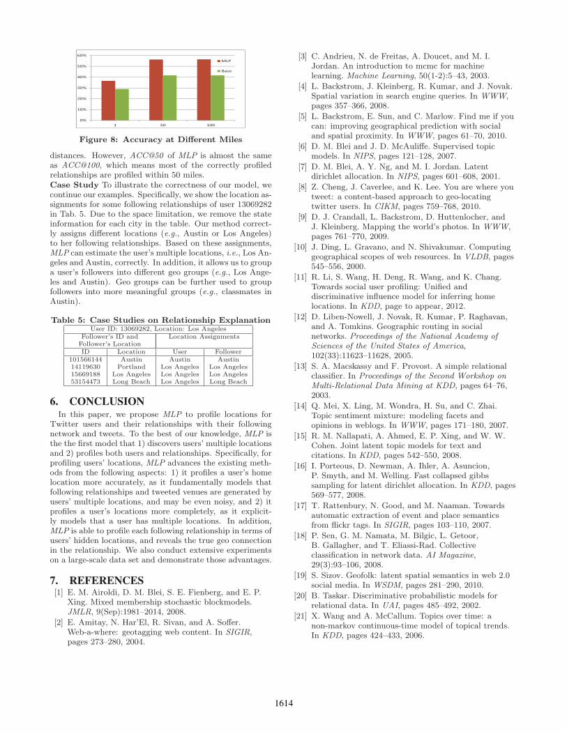
Figure 8: Accuracy at Different Miles

distances. However, ACC@50 of MLP is almost the sameas ACC@100, which means most of the correctly profiledrelationships are profiled within 50 miles.Case Study To illustrate the correctness of our model, wecontinue our examples. Specifically, we show the location as-signments for some following relationships of user 13069282in Tab. 5. Due to the space limitation, we remove the stateinformation for each city in the table. Our method correct-ly assigns different locations (e.g., Austin or Los Angeles)to her following relationships. Based on these assignments,MLP can estimate the user’s multiple locations, i.e., Los An-geles and Austin, correctly. In addition, it allows us to groupa user’s followers into different geo groups (e.g., Los Ange-les and Austin). Geo groups can be further used to groupfollowers into more meaningful groups (e.g., classmates inAustin).

Table 5: Case Studies on Relationship ExplanationUser ID: 13069282, Location: Los Angeles

Follower’s ID and Location AssignmentsFollower’s LocationID Location User Follower

101566144 Austin Austin Austin14119630 Portland Los Angeles Los Angeles15669188 Los Angeles Los Angeles Los Angeles53154473 Long Beach Los Angeles Long Beach

6. CONCLUSIONIn this paper, we propose MLP to profile locations for

Twitter users and their relationships with their followingnetwork and tweets. To the best of our knowledge, MLP isthe the first model that 1) discovers users’ multiple locationsand 2) profiles both users and relationships. Specifically, forprofiling users’ locations, MLP advances the existing meth-ods from the following aspects: 1) it profiles a user’s homelocation more accurately, as it fundamentally models thatfollowing relationships and tweeted venues are generated byusers’ multiple locations, and may be even noisy, and 2) itprofiles a user’s locations more completely, as it explicit-ly models that a user has multiple locations. In addition,MLP is able to profile each following relationship in terms ofusers’ hidden locations, and reveals the true geo connectionin the relationship. We also conduct extensive experimentson a large-scale data set and demonstrate those advantages.

7. REFERENCES[1] E. M. Airoldi, D. M. Blei, S. E. Fienberg, and E. P.

Xing. Mixed membership stochastic blockmodels.JMLR, 9(Sep):1981–2014, 2008.

[2] E. Amitay, N. Har’El, R. Sivan, and A. Soffer.Web-a-where: geotagging web content. In SIGIR,pages 273–280, 2004.

[3] C. Andrieu, N. de Freitas, A. Doucet, and M. I.Jordan. An introduction to mcmc for machinelearning. Machine Learning, 50(1-2):5–43, 2003.

[4] L. Backstrom, J. Kleinberg, R. Kumar, and J. Novak.Spatial variation in search engine queries. In WWW,pages 357–366, 2008.

[5] L. Backstrom, E. Sun, and C. Marlow. Find me if youcan: improving geographical prediction with socialand spatial proximity. In WWW, pages 61–70, 2010.

[6] D. M. Blei and J. D. McAuliffe. Supervised topicmodels. In NIPS, pages 121–128, 2007.

[7] D. M. Blei, A. Y. Ng, and M. I. Jordan. Latentdirichlet allocation. In NIPS, pages 601–608, 2001.

[8] Z. Cheng, J. Caverlee, and K. Lee. You are where youtweet: a content-based approach to geo-locatingtwitter users. In CIKM, pages 759–768, 2010.

[9] D. J. Crandall, L. Backstrom, D. Huttenlocher, andJ. Kleinberg. Mapping the world’s photos. In WWW,pages 761–770, 2009.

[10] J. Ding, L. Gravano, and N. Shivakumar. Computinggeographical scopes of web resources. In VLDB, pages545–556, 2000.

[11] R. Li, S. Wang, H. Deng, R. Wang, and K. Chang.Towards social user profiling: Unified anddiscriminative influence model for inferring homelocations. In KDD, page to appear, 2012.

[12] D. Liben-Nowell, J. Novak, R. Kumar, P. Raghavan,and A. Tomkins. Geographic routing in socialnetworks. Proceedings of the National Academy of

Sciences of the United States of America,102(33):11623–11628, 2005.

[13] S. A. Macskassy and F. Provost. A simple relationalclassifier. In Proceedings of the Second Workshop on

Multi-Relational Data Mining at KDD, pages 64–76,2003.

[14] Q. Mei, X. Ling, M. Wondra, H. Su, and C. Zhai.Topic sentiment mixture: modeling facets andopinions in weblogs. In WWW, pages 171–180, 2007.

[15] R. M. Nallapati, A. Ahmed, E. P. Xing, and W. W.Cohen. Joint latent topic models for text andcitations. In KDD, pages 542–550, 2008.

[16] I. Porteous, D. Newman, A. Ihler, A. Asuncion,P. Smyth, and M. Welling. Fast collapsed gibbssampling for latent dirichlet allocation. In KDD, pages569–577, 2008.

[17] T. Rattenbury, N. Good, and M. Naaman. Towardsautomatic extraction of event and place semanticsfrom flickr tags. In SIGIR, pages 103–110, 2007.

[18] P. Sen, G. M. Namata, M. Bilgic, L. Getoor,B. Gallagher, and T. Eliassi-Rad. Collectiveclassification in network data. AI Magazine,29(3):93–106, 2008.

[19] S. Sizov. Geofolk: latent spatial semantics in web 2.0social media. In WSDM, pages 281–290, 2010.

[20] B. Taskar. Discriminative probabilistic models forrelational data. In UAI, pages 485–492, 2002.

[21] X. Wang and A. McCallum. Topics over time: anon-markov continuous-time model of topical trends.In KDD, pages 424–433, 2006.

1614