Multiple Antennas in Wireless Communications:

Array Signal Processing and Channel Capacity

by

Mahesh Godavarti

A dissertation submitted in partial fulfillmentof the requirements for the degree of

Doctor of Philosophy(Electrical Engineering: Systems)in The University of Michigan

2001

Doctoral Committee:

Professor Alfred O. Hero, III, ChairAssociate Professor Kamal SarabandiProfessor Wayne E. StarkAssociate Professor Kim Winick

ABSTRACT

Multiple Antennas in Wireless Communications: Array Signal Processing and Channel Capacity

byMahesh Godavarti

Chair: Alfred O. Hero, III

We investigate two aspects of multiple-antenna wireless communication systems

in this thesis: 1) deployment of an adaptive beamformer array at the receiver; and

2) space-time coding for arrays at the transmitter and the receiver. In the first

part of the thesis, we establish sufficient conditions for the convergence of a popular

least mean squares (LMS) algorithm known as the sequential Partial Update LMS

Algorithm for adaptive beamforming. Partial update LMS (PU-LMS) algorithms

are reduced complexity versions of the full update LMS that update a subset of

filter coefficients at each iteration. We introduce a new improved algorithm, called

Stochastic PU-LMS, which selects the subsets at random at each iteration. We

show that the new algorithm converges for a wider class of signals than the existing

PU-LMS algorithms.

The second part of this thesis deals with the multiple-input multiple-output

(MIMO) Shannon capacity of multiple antenna wireless communication systems un-

der the average energy constraint on the input signal. Previous work on this problem

has concentrated on capacity for Rayleigh fading channels. We investigate the more

general case of Rician fading. We derive capacity expressions, optimum transmit sig-

nals as well as upper and lower bounds on capacity for three Rician fading models. In

the first model the specular component is a dynamic isotropically distributed random

process. In this case, the optimum transmit signal structure is the same as that for

Rayleigh fading. In the second model the specular component is a static isotropically

distributed random process unknown to the transmitter, but known to the receiver.

In this case the transmitter has to design the transmit signal to guarantee a cer-

tain rate independent of the specular component. Here also, the optimum transmit

signal structure, under the constant magnitude constraint, is the same as that for

Rayleigh fading. In the third model the specular component is deterministic and

known to both the transmitter and the receiver. In this case the optimum transmit

signal and capacity both depend on the specular component. We show that for low

signal to noise ratio (SNR) the specular component completely determines the the

signal structure whereas for high SNR the specular component has no effect. We also

show that training is not effective at low SNR and give expressions for rate-optimal

allocation of training versus communication.

c©Mahesh Godavarti 2001

All Rights Reserved

To my family and friends

ii

ACKNOWLEDGEMENTS

I would like to extend my sincere thanks to my advisor Prof. Alfred O. Hero-III

for letting me dictate the pace of my research, giving me freedom to a large extent

on the choice of topics, his invaluable guidance and encouragement, and for giving

me invaluable insight into my research.

I would also like to extend my thanks to Dr. Thomas Marzetta at Bell Labs,

Murray Hill, NJ for supervising my summer internship and helping me develop a

significant part of my thesis.

I am grateful to my committee members, Professor Wayne Stark, Associate Profes-

sor Kim Winick and Associate Professor Kamal Sarabandi for their valuable inputs.

I am also thankful to them, especially Dr. Sarabandi, for being gracious enough to

accommodate me and making the final oral defense possible on the day of my choice.

I would like to thank my friends, Olgica Milenkovic, Dejan Filipovic, Tara Javidi,

Victoria Yee, Riten Gupta, Robinson Piramuthu, Bing Ma, Tingfang Ji, John Choi,

Ketan Patel, Sungill Kim, Selin Aviyente, Jia Li, Ali Ozgur and Rajiv Vijayakumar

for making my experiences in the department pleasant; Zoya Khan and Madhumati

Ramesh for being great neighbours; Sivakumar Santhanakrishnan for being an un-

derstanding roommate; and Bhavani Raman and Muralikrishna Datla for making

my experience in SPICMACAY rewarding.

A special thanks to Navin Kashyap for being a sounding board.

My sincere thanks to Department of Defense Research & Engineering (DDR&E)

iii

Multidisciplinary University Research Initiative (MURI) on “Low Energy Electron-

ics Design for Mobile Platform” managed by the Army Research Office (ARO) for

supporting this research through ARO grant DAAH04-96-1-0337. My thanks to the

Department of Electrical Engineering as well for supporting this research through

various fellowships and Assistantships.

Finally, I would like to thank my parents, brother and sister who have always

encouraged me in my quest for higher education and especially my wife and friend

of many years Kavita Raman for encouraging me and listening to my occasional

laments and for supporting my many decisions.

iv

TABLE OF CONTENTS

DEDICATION . . . . . . . . . . . . . . . . . . . . . . . . . . . . . . . . . . . . . . . . . . ii

ACKNOWLEDGEMENTS . . . . . . . . . . . . . . . . . . . . . . . . . . . . . . . . . . iii

LIST OF FIGURES . . . . . . . . . . . . . . . . . . . . . . . . . . . . . . . . . . . . . . vii

LIST OF APPENDICES . . . . . . . . . . . . . . . . . . . . . . . . . . . . . . . . . . . ix

CHAPTER

1. Introduction . . . . . . . . . . . . . . . . . . . . . . . . . . . . . . . . . . . . . . . 1

1.1 Partial Update LMS Algorithms . . . . . . . . . . . . . . . . . . . . . . . . . 71.2 Multiple-Antenna Capacity . . . . . . . . . . . . . . . . . . . . . . . . . . . . 91.3 Organization of the Dissertation and Significant Contributions . . . . . . . . 12

2. Sequential Partial Update LMS Algorithm . . . . . . . . . . . . . . . . . . . . 16

2.1 Introduction . . . . . . . . . . . . . . . . . . . . . . . . . . . . . . . . . . . . 162.2 Algorithm Description . . . . . . . . . . . . . . . . . . . . . . . . . . . . . . . 182.3 Analysis: Stationary Signals . . . . . . . . . . . . . . . . . . . . . . . . . . . 192.4 Analysis: Cyclo-stationary Signals . . . . . . . . . . . . . . . . . . . . . . . . 232.5 Example . . . . . . . . . . . . . . . . . . . . . . . . . . . . . . . . . . . . . . 252.6 Conclusion . . . . . . . . . . . . . . . . . . . . . . . . . . . . . . . . . . . . . 26

3. Stochastic Partial Update LMS Algorithm . . . . . . . . . . . . . . . . . . . . 30

3.1 Introduction . . . . . . . . . . . . . . . . . . . . . . . . . . . . . . . . . . . . 303.2 Algorithm Description . . . . . . . . . . . . . . . . . . . . . . . . . . . . . . . 313.3 Analysis of SPU-LMS: Stationary Stochastic Signals . . . . . . . . . . . . . . 323.4 Analysis SPU-LMS: Deterministic Signals . . . . . . . . . . . . . . . . . . . . 353.5 General Analysis of SPU-LMS . . . . . . . . . . . . . . . . . . . . . . . . . . 363.6 Periodic and Sequential LMS Algorithms . . . . . . . . . . . . . . . . . . . . 433.7 Simulation of an Array Examples to Illustrate the advantage of SPU-LMS . 443.8 Examples . . . . . . . . . . . . . . . . . . . . . . . . . . . . . . . . . . . . . . 483.9 Conclusion and Future Work . . . . . . . . . . . . . . . . . . . . . . . . . . . 51

4. Capacity: Isotropically Random Rician Fading . . . . . . . . . . . . . . . . . 53

4.1 Introduction . . . . . . . . . . . . . . . . . . . . . . . . . . . . . . . . . . . . 534.2 Signal Model . . . . . . . . . . . . . . . . . . . . . . . . . . . . . . . . . . . . 544.3 Properties of Capacity Achieving Signals . . . . . . . . . . . . . . . . . . . . 574.4 Capacity Upper and Lower Bounds . . . . . . . . . . . . . . . . . . . . . . . 594.5 Numerical Results . . . . . . . . . . . . . . . . . . . . . . . . . . . . . . . . . 62

v

4.6 Analysis for High SNR . . . . . . . . . . . . . . . . . . . . . . . . . . . . . . 634.7 Conclusions . . . . . . . . . . . . . . . . . . . . . . . . . . . . . . . . . . . . 65

5. Min-Capacity: Rician Fading, Unknown Static Specular Component . . . 66

5.1 Introduction . . . . . . . . . . . . . . . . . . . . . . . . . . . . . . . . . . . . 665.2 Signal Model and Min-Capacity Criterion . . . . . . . . . . . . . . . . . . . . 685.3 Capacity Upper and Lower Bounds . . . . . . . . . . . . . . . . . . . . . . . 695.4 Properties of Capacity Achieving Signals . . . . . . . . . . . . . . . . . . . . 725.5 Average Capacity Criterion . . . . . . . . . . . . . . . . . . . . . . . . . . . . 755.6 Coding Theorem for Min-capacity . . . . . . . . . . . . . . . . . . . . . . . . 785.7 Numerical Results . . . . . . . . . . . . . . . . . . . . . . . . . . . . . . . . . 805.8 Conclusions . . . . . . . . . . . . . . . . . . . . . . . . . . . . . . . . . . . . 80

6. Capacity: Rician Fading, Known Static Specular Component . . . . . . . . 83

6.1 Introduction . . . . . . . . . . . . . . . . . . . . . . . . . . . . . . . . . . . . 836.2 Rank-one Specular Component . . . . . . . . . . . . . . . . . . . . . . . . . . 846.3 General Rank Specular Component . . . . . . . . . . . . . . . . . . . . . . . 886.4 Training in Non-Coherent Communications . . . . . . . . . . . . . . . . . . . 1036.5 Conclusions and Future Work . . . . . . . . . . . . . . . . . . . . . . . . . . 119

7. Diversity versus Degrees of Freedom . . . . . . . . . . . . . . . . . . . . . . . . 121

7.1 Introduction . . . . . . . . . . . . . . . . . . . . . . . . . . . . . . . . . . . . 1217.2 Examples . . . . . . . . . . . . . . . . . . . . . . . . . . . . . . . . . . . . . . 1247.3 Conclusions . . . . . . . . . . . . . . . . . . . . . . . . . . . . . . . . . . . . 133

APPENDICES . . . . . . . . . . . . . . . . . . . . . . . . . . . . . . . . . . . . . . . . . . 134

BIBLIOGRAPHY . . . . . . . . . . . . . . . . . . . . . . . . . . . . . . . . . . . . . . . . 178

vi

LIST OF FIGURES

Figure

1.1 Diagram of a multiple antenna communication system . . . . . . . . . . . . . . . . 11

2.1 Block diagram of S-LMS for the special case of alternating even/odd coefficientupdate . . . . . . . . . . . . . . . . . . . . . . . . . . . . . . . . . . . . . . . . . . . 28

2.2 Trajectory of w1,k and w2,k for µ = 0.33 . . . . . . . . . . . . . . . . . . . . . . . . 28

2.3 Trajectory of w1,k and w2,k for µ = 0.0254 . . . . . . . . . . . . . . . . . . . . . . . 29

3.1 Signal Scenario for Example 1 . . . . . . . . . . . . . . . . . . . . . . . . . . . . . . 45

3.2 Trajectories of MSE for Example 1 . . . . . . . . . . . . . . . . . . . . . . . . . . . 46

3.3 Signal Scenario for Example 2 . . . . . . . . . . . . . . . . . . . . . . . . . . . . . . 47

3.4 Trajectories of MSE for Example 2 . . . . . . . . . . . . . . . . . . . . . . . . . . . 48

4.1 Capacity and Capacity lower bound for M = N = 1 as T →∞ . . . . . . . . . . . 62

4.2 Capacity upper and lower bounds as the channel moves from purely Rayleigh topurely Rician fading . . . . . . . . . . . . . . . . . . . . . . . . . . . . . . . . . . . 63

4.3 Capacity upper and lower bounds as the channel moves from purely Rayleigh topurely Rician fading . . . . . . . . . . . . . . . . . . . . . . . . . . . . . . . . . . . 64

4.4 Capacity and capacity lower bound as a function of SNR for a purely Rayleighfading channel . . . . . . . . . . . . . . . . . . . . . . . . . . . . . . . . . . . . . . . 64

5.1 Capacity upper and lower bounds as the channel moves from purely Rayleigh topurely Rician fading . . . . . . . . . . . . . . . . . . . . . . . . . . . . . . . . . . . 81

5.2 Capacity upper and lower bounds as the channel moves from purely Rayleigh topurely Rician fading . . . . . . . . . . . . . . . . . . . . . . . . . . . . . . . . . . . 81

6.1 Optimum value of d as a function of r for different values of ρ . . . . . . . . . . . . 88

6.2 Asymptotic capacity upper bound, Capacity Upper and Lower bounds for differentvalues of SNR . . . . . . . . . . . . . . . . . . . . . . . . . . . . . . . . . . . . . . . 105

6.3 Plot of rnew as a function of Rician parameter r . . . . . . . . . . . . . . . . . . . . 112

6.4 Plot of optimal energy allocation κ as a function of Rician parameter r . . . . . . . 112

vii

6.5 Plot of optimal power allocation as a function of T . . . . . . . . . . . . . . . . . . 113

6.6 Plot of capacity as a function of number of transmit antennas for a fixed T . . . . 113

6.7 Optimal Tt as a function of T for equal transmit and training powers . . . . . . . . 114

6.8 Comparison of the two lower bounds for dB = −20 . . . . . . . . . . . . . . . . . . 118

6.9 Comparison of the two lower bounds for dB = 0 . . . . . . . . . . . . . . . . . . . . 118

6.10 Comparison of the two lower bounds for dB = 20 . . . . . . . . . . . . . . . . . . . 119

7.1 DOF as a function of DIV . . . . . . . . . . . . . . . . . . . . . . . . . . . . . . . . 130

viii

LIST OF APPENDICES

Appendix

A. Appendices for Chapter 3 . . . . . . . . . . . . . . . . . . . . . . . . . . . . . . . . . . 135A.1 Derivation of Stability Condition (3.7) . . . . . . . . . . . . . . . . . . . . . 135A.2 Derivation of expression (3.9) . . . . . . . . . . . . . . . . . . . . . . . . . . . 136A.3 Derivation of the misadjustment factor (3.8) . . . . . . . . . . . . . . . . . . 137A.4 Proofs of Lemma 3.1 and Theorem 3.1 . . . . . . . . . . . . . . . . . . . . . 137A.5 Proof of Theorem 3.2 in Section 3.5.1 . . . . . . . . . . . . . . . . . . . . . . 141A.6 Derivation of Expressions in Section 3.8.1 . . . . . . . . . . . . . . . . . . . . 146A.7 Derivation of Expressions in Section 3.3 . . . . . . . . . . . . . . . . . . . . . 150

B. Appendices for Chapter 6 . . . . . . . . . . . . . . . . . . . . . . . . . . . . . . . . . . 154B.1 Capacity Optimization in Section 6.2.1 . . . . . . . . . . . . . . . . . . . . . 154B.2 Non-coherent Capacity for low SNR values under Peak Power Constraint . . 155B.3 Proof of Lemma 6.3 in Section 6.3.4 . . . . . . . . . . . . . . . . . . . . . . . 157B.4 Convergence of Entropies . . . . . . . . . . . . . . . . . . . . . . . . . . . . . 166B.5 Convergence of H(X) for T > M = N needed in the proof of Theorem 6.4

in Section 6.3.4 . . . . . . . . . . . . . . . . . . . . . . . . . . . . . . . . . . 171B.6 Proof of Theorem 6.7 in Section 6.4.1 . . . . . . . . . . . . . . . . . . . . . . 174B.7 Proof of Theorem 6.8 in Section 6.4.1 . . . . . . . . . . . . . . . . . . . . . . 175B.8 Proof of Theorem 6.9 in Section 6.4.1 . . . . . . . . . . . . . . . . . . . . . . 177

ix

CHAPTER 1

Introduction

This thesis deals with theory underlying the deployment of multiple antennas, i.e.

antenna arrays, at transmitter and receiver for the purpose of improved communi-

cation, reliability and performance. The thesis can be divided into two main parts.

The first part deals with conditions for convergence of adaptive receiver arrays and a

new reduced complexity beamformer algorithm. The second part deals with channel

capacity for a Rician fading multiple-input multiple-output (MIMO) channel. More

details are given in the rest of this chapter.

Wireless communications have been gaining popularity because of better antenna

technologies, lower costs, easier deployment of wireless systems, greater flexibility,

better reliability and the need for mobile communication. In some cases, like in very

remote areas, wireless connections may be the only option.

Even though the popularity of mobile wireless telephony and paging is a recent

phenomenon, fixed-wireless systems have a long history. Point-to-point microwave

connections have long been used for voice and data communications, generally in

backhaul networks operated by phone companies, cable TV companies, utilities,

railways, paging companies and government agencies, and will continue to be an

important part of the communications infrastructure. Improvements in technology

1

2

have allowed higher frequencies and thus smaller antennas to be used resulting in

lower costs and easier-to-deploy systems.

Another reason for the popularity of wireless systems is that consumers demand

for data rates has been insatiable. Wireline models have topped off at a rate of

56Kbps and end-users have been looking for integrated digital subscriber network

(ISDN) and digital subscriber line (DSL) connections. Companies with T1 connec-

tions of 1.54Mbps have found the connections inadequate and are turning to T3

optical fiber connections. The very expensive deployment of fiber connections, how-

ever, has caused companies to turn to fixed wireless links.

This has resulted in the application of wireless communications to a host of ap-

plications ranging from: fixed microwave links; wireless local area networks (LANs);

data over cellular networks; wireless wide area networks (WANs); satellite links;

digital dispatch networks; one-way and two-way paging networks; diffuse infrared;

laser-based communications; keyless car entry; the Global Positioning System (GPS);

mobile cellular communications; and indoor-radio.

One challenge in wireless systems not present in wireline systems is the issue of

fading. Fading arises due to the possible existence of multiple paths from the trans-

mitter to the receiver with destructive combination at the receiver output. There are

many models describing fading in wireless channels [20]. The classic models being

Rayleigh and Rician flat fading models. Rayleigh and Rician models are typically

applied to narrowband signals and do not include the doppler shift induced by the

motion of the transmitter or the receiver.

In wireless systems, there are three different ways to combat fading: 1) frequency

diversity; 2) time diversity; and 3) spatial diversity. Frequency diversity makes use of

the fact that multipath structure in different frequency bands is different. This fact

3

can be exploited to mitigate the effect of fading. But, the positive effects of frequency

diversity are limited due to bandwidth limitations. Wireless communication uses

radio spectrum, a finite resource. This limits the number of wireless users and the

amount of spectrum available to any user at any moment in time. Time diversity

makes use of the fact that fading over different time intervals is different. By using

channel coding the effect of bad fading intervals can be mitigated by good fading

intervals. However, due to delay constraints time diversity is difficult to exploit.

Spatial diversity exploits multiple antennas either separated in space or differently

polarized [7, 23, 24]. Different antennas see different multipath characteristics or

different fading characteristics and this can be used to generate a stronger signal.

Spatial diversity techniques do not have the drawbacks associated with time diversity

and frequency diversity techniques. The one drawback of spatial diversity is that it

involves deployment of multiple antennas at the transmitter and the receiver which

is not always feasible.

In this thesis, we will concentrate on spatial diversity resulting from deployment

of multiple antennas. Spatial diversity, at the receiver (multiple antennas at the

receiver) or at the transmitter (multiple antennas at the transmitter), can improve

link performance in the following ways [31]

1. Improvements in spectrum efficiency: Multiple antennas can be used to accom-

modate more than one user in a given spectral bandwidth.

2. Extension of range coverage: Multiple antennas can be used to direct the energy

of a signal in a given direction and hence minimize leakage of signal energy.

3. Tracking of multiple mobiles: The outputs of antennas can be combined in

different ways to isolate signals from each and every mobile.

4

4. Increases in channel reuse: Improving spectral efficiency can allow more than

one user to operate in a cell.

5. Reductions in power usage: By directing the energy in a certain direction and

increasing range coverage lesser energy can be used to reach a user at a given

distance.

6. Generation of multiple access: Appropriately combining the outputs of the an-

tennas can selectively provide access to users.

7. Reduction of co-channel interference

8. Combating of fading

9. Increase in information channel capacity: Multiple antennas have been used to

increase the maximum achievable data rates.

Traditionally, all the gains listed above have been realized by explicitly directing

the receive or transmit antenna array to point in specific directions. This process is

called beamforming. For receive antennas, beamforming can be achieved electroni-

cally by appropriately weighting the antenna outputs and combining them to make

the antenna response to energy emanating from certain directions more sensitive than

others. Until recently most of the research on antenna arrays for beamforming has

dealt with beamformers at the receiver. Transmit beamformers behave differently

and require different algorithms and hardware [32].

Methods of beamforming at the receive antenna array currently in use are based

on array processing algorithms for signal copy, direction finding and signal separation

[32]. These include Applebaum/Frost beamforming, null steering beamforming, opti-

mal beamforming, beam-space Processing, blind beamforming, optimum combining

5

and maximal ratio combining [15, 32, 64, 68, 69, 74, 80]. Many of these beamform-

ers require a reference signal and use adaptive algorithms to optimize beamformer

weights with respect to some beamforming performance criterion [32, 78, 79, 81].

Adaptive algorithms can also be used without training for tracking a time varying

mobile user, tracking multiple users, or tracking time varying channels. Popular

examples [32] are the Least Mean Squares Algorithm (LMS), Constant Modulus

Algorithm (CMA) and the Recursive Least Squares (RLS) algorithm. The algorithm

of interest in this work is the LMS Algorithm because of its ease of implementation

and low complexity.

Another research topic in the field of beamforming that has generated much in-

terest is the effect of calibration errors in direction finding and signal copy problems

[25, 49, 65, 66, 67, 83, 84]. An array with Gaussian calibration errors operating in

a non-fading environment has the same model as a Rician fading channel. Thus

the work done in this thesis can be easily translated to the case of array calibration

errors.

Beamforming at the receiver is one way of exploiting receive diversity. Most pre-

vious work (1995 and earlier) in the literature concentrates on this kind of diversity.

Another way to exploit diversity is to perform beamforming at the transmitter, i.e.

transmit diversity. Beamforming at the transmitter increases the signal to noise ratio

(SNR) at the receiver by focusing the transmit energy in the directions that ensures

the strongest reception at the receiver. Exploitation of transmit diversity can in-

volve [71] using the channel state information obtained via feedback for reassigning

energy at different antennas via waterpouring, linear processing of signals to spread

the information across transmit antennas and using channel codes and transmitting

the codes using different antennas in an orthogonal manner.

6

An early use of the multiple transmit antennas was to obtain diversity gains by

sending multiple copies of a signal over orthogonal time or frequency slices (rep-

etition code). This of course, incurs a bandwidth expansion factor equal to the

number of antennas. A transmit diversity technique without bandwidth expansion

was first suggested by Wittenben [82]. Wittenben’s diversity technique of sending

time-delayed copies of a common input signal over transmit multiple antennas was

also independently discovered by Seshadri and Winters [58] and by Weerackody [77].

An information theoretic approach to designing transmit diversity schemes was un-

dertaken by Narula [53, 54]. The authors design schemes that maximize the mutual

information between the transmitter and the receiver.

These methods correspond to beamforming where knowledge of the channel is

available at the transmitter and receiver, for example by training and feedback. In

such a case the strategy is to mitigate the effect of multipath by spatial diversity and

focusing the channel to a single equivalent direct path channel by beamforming.

Recently, researchers have realized that beamforming may not be the optimal

way to increase data rates. The BLAST project showed that multipaths are not as

harmful as previously thought and that the multiple diversity can be exploited to

increase capacity even when the channel is unknown [23, 50]. This has given rise to

research on space-time codes [8, 42, 43, 47, 48, 52, 70, 71]. Space-time coding is a

coding technique that is designed for use with multiple transmit antennas. One of

the first papers in this area is by Alamouti [5] who designed a simple scheme for a

two-antenna transmit system. The codes are designed to induce spatial and temporal

correlations into signals that are robust to unknown channel variations and can be

exploited at the receiver. Space-time codes are simply a systematic way to perform

beneficial space-time processing of signals before transmission [52].

7

Design of space-time codes has taken many forms. Tarokh et. al. [70, 71] have

taken an approach to designing space-time codes for both Rayleigh and Rician fading

channels with complete channel state information at the receiver that maximizes a

pairwise codeword distance criterion. The pairwise distance criterion was derived

from an upper bound on probability of decoding error. There have also been code

designs where the receiver has no knowledge about the MIMO channel. Hero and

Marzetta [42] design space-time codes with a design criterion of maximizing the cut-

off rate for the MIMO Rayleigh fading channel. Hochwald et. al [43, 44] propose a

design based on signal structures that asymptotically achieve capacity in the non-

coherent case for MIMO Rayleigh fading channels. Hughes [47, 48] considered the

design of space-time based on the concept of Group codes. The codes can be viewed

as an extended version of phase shift keying for the case of multiple antenna com-

munications. In [47] the author independently proposed a scheme similar to that

proposed by Hochwald and Marzetta in [43]. More recent work in this area has

been by Hassibi on linear dispersion codes [38] and fixed-point free codes [40] and by

Shokrollahi on double diagonal space-time codes [61] and unitary space-time codes

[62].

The research reported in this dissertation concentrates on adaptive beamforming

receivers for fixed deterministic channels and channel capacity of multiple antennas

in the presence of Rician fading. We will elaborate more on the research contributions

in the following sections.

1.1 Partial Update LMS Algorithms

The LMS algorithm is a popular algorithm for adaptation of weights in adap-

tive beamformers using antenna arrays and for channel equalization to combat in-

8

tersymbol interference. Many others application areas of LMS include interference

cancellation, echo cancellation, space time modulation and coding and signal copy

in surveillance. Although there exist algorithms with faster convergence rates like

RLS, LMS is very popular because of ease of implementation and low computational

costs.

One of the variants of LMS is the Partial Update LMS (PU-LMS) Algorithm.

Some of the applications in wireless communications like channel equalization and

echo cancellation require the adaptive filter to have a very large number of coeffi-

cients. Updating of the entire coefficient set might be beyond the ability of the mobile

units. Therefore, partial updating of the LMS adaptive filter has been proposed to

further reduce computational costs [30, 33, 51]. In this era of mobile computing

and communications, such implementations are also attractive for reducing power

consumption. However, theoretical performance predictions on convergence rate and

steady state tracking error are more difficult to derive than for standard full update

LMS. Accurate theoretical predictions are important as it has been observed that

the standard LMS conditions on the step size parameter fail to ensure convergence

of the partial update algorithm.

Two of the partial update algorithms prevalent in the literature have been de-

scribed in [18]. They are referred to as the “Periodic LMS algorithm” and the

“Sequential LMS algorithm”. To reduce computation by a factor of P , the Periodic

LMS algorithm (P-LMS) updates all the filter coefficients every P th iteration instead

of every iteration. The Sequential LMS (S-LMS) algorithm updates only a fraction

of coefficients every iteration.

Another variant referred to as “Max Partial Update LMS algorithm” (Max PU-

LMS) has been proposed in [16, 17] and [3]. In this algorithm, the subset of coeffi-

9

cients to be updated is dependent on the input signal. The subset is chosen so as to

minimize the increase in the mean squared error due to partial as opposed to full up-

dating. The input signals multiplying each coefficient are ordered according to their

magnitude and the coefficients corresponding to the largest 1P

of input signals are

chosen for update in an iteration. Some analysis of this algorithm has been done in

[17] for the special case of one coefficient per iteration but, analysis for more general

cases still needs to be completed. The results on stochastic updating in Chapter 3

provide a small step in this direction.

1.2 Multiple-Antenna Capacity

Shannon in his famous paper [59] showed that it is possible to communicate over

a noisy channel with arbitrary reliability provided that the amount of information

communicated (bits/channel use) is less than a constant. This constant is known as

the channel capacity. Shannon showed that the channel capacity can be computed

by maximizing the mutual information between the input and the output over all

possible input distributions. The channel capacity for a range of channels like the

binary symmetric channel, the additive white Gaussian noise (AWGN) channel have

already been computed in the literature [13, 26]. Computing the capacity for more

complicated channels like Rayleigh fading and Rician fading channels is in general a

difficult problem.

The seminal paper by Foschini et. al. [23, 24] showed that a significant gain

in capacity can be achieved by using multiple antennas in the presence of Rayleigh

fading. LetM be the number of antennas at the transmitter and N be the number of

antennas at the receiver. Foschini and Telatar showed [73] that with perfect channel

knowledge at the receiver, for high SNR a capacity gain of min(M,N) bits/second/Hz

10

can be achieved with every 3 dB increase in SNR. Channel knowledge at the receiver

however requires that the time between different fades be sufficiently large to enable

the receiver to learn the channel via training. This might not be true in the case of

fast mobile receivers and large numbers of transmit antennas. Furthermore, the use

of training is an overhead which reduces the attainable capacity.

Following Foschini [23], there have been many papers written on the subject of

calculating capacity for a MIMO channel [7, 10, 12, 28, 29, 34, 35, 50, 60, 72, 76].

Others have studied the achievable rate regions for the MIMO channel in terms of

cut-off rate [42] and error exponents [1].

Marzetta and Hochwald [50] considered a Rayleigh fading MIMO channel when

neither the receiver nor the transmitter has any knowledge of the fading coefficients.

In their model the fading coefficients remain constant for T symbol periods and

instantaneously change to new independent complex Gaussian realizations every T

symbol periods. They established that to achieve capacity it is sufficient to use

M = T antennas at the transmitter and that the capacity achieving signal matrix

consists of a product of two independent matrices, a T × T isotropically random

unitary matrix and a T ×M real nonnegative diagonal matrix. Hence, it is sufficient

to optimize over the density of a smaller parameter set of size minM,T instead of

the original parameter set of size T ·M .

Zheng and Tse [85] derived explicit capacity results for the case of high SNR in

the case of no channel knowledge at the transmitter or receiver. They showed that

the number of degrees of freedom for non-coherent communication is M ∗(1−M ∗/T )

where M ∗ = minM,N, T/2 as opposed to minM,N in the case of coherent

communications.

The literature cited above has limited its attention to Rayleigh fading channel

11

models for computing capacity of multiple-antenna wireless links. However, Rayleigh

fading models are inadequate in describing the many fading channels encountered

in practice. Another popular model used in the literature to fill this gap is the

Rician fading channel. Rician fading is a more accurate model when there are some

direct paths present between the transmitter and the receiver along with the diffuse

multipath (Figure 1.1). Rician fading components traditionally have been modeled

Rank One Specular Component

M-Transmit Antennas N-Receive AntennasIndependent Paths (Possibly over time)

Post-Processing N

Post-Processing 2

Post-Processing 1Pre-Processing 1

Pre-Processing 2

Pre-Processing M

ReceivedInformationInformation to

be Transmitted

Figure 1.1: Diagram of a multiple antenna communication system

as independent Gaussian components with a deterministic non-zero mean [9, 19,

21, 56, 57, 71]. Farrokhi et. al. [21] used this model to analyze the capacity of

a MIMO channel with a single specular component. In their paper they assumed

that the specular component is static and unknown to the transmitter but known

to the receiver. They also assumed that the receiver has complete knowledge about

the fading coefficients (i.e. the Rayleigh and specular components are completely

known). They work with the premise that since the transmitter has no knowledge

about the specular component the signaling scheme has to be designed to guarantee

a given rate irrespective of the value of the specular component. They conclude

12

that the signal matrix has to be composed of independent circular Gaussian random

variables of mean 0 and equal variance in order to maximize the rate and achieve

capacity.

1.3 Organization of the Dissertation and Significant Contributions

In this work, we have made the following contributions. These contributions

are divided into two fields: 1) LMS algorithm convergence for adaptive arrays at

the receiver; and 2) evaluation of Shannon capacity for multiple antennas at the

transmitter and the receiver in the presence of Rician fading.

1. In Chapter 2 we analyze the Sequential PU-LMS for stability and come up

with more stringent conditions on stability than were previously known. We

illustrate our findings via simulations.

• Contributions: Derived conditions ensuring the stability of the Sequential

PU-LMS algorithm for stationary signals without the restrictive assump-

tions of [18]. The analysis of the algorithm for cyclo-stationary signals

establishes that the deterministic sequences of updates is the reason be-

hind the algorithm’s poor convergence. This motivates a new Stochastic

PU-LMS, a more stable algorithm.

2. Chapter 3 analyzes the Stochastic Partial Update LMS algorithm where the

coefficients to be updated in an iteration are chosen at random. This generalizes

the previous PU-LMS methods. We derive conditions for stability and also

analyze the algorithm for performance. We demonstrate the effectiveness of our

analysis via simulations.

• Contributions: Proposed a new Partial Update algorithm with better con-

13

vergence properties than those of existing Partial Update LMS algorithms.

The convergence of Stochastic PU-LMS is better than the existing PU-LMS

algorithms for the case of non-stationary signals and similar to the exist-

ing algorithms for the case of stationary signals. The analysis elucidates

the role of parameters which determine the convergence or divergence of

PU-LMS algorithms.

Contributions reported in the subsequent chapters have been in the area of

computing capacity for a more general fading model than the Rayleigh model.

This we consider is the first significant step towards computing capacities for

more realistic models for MIMO systems.

3. In Chapter 4, we introduce a MIMO Rician fading where the specular component

is also modeled as dynamic and random but, with an isotropically uniform

density [50]. With this model the channel capacity can be easily characterized.

We also derive a lower bound to capacity which is useful to establish achievable

rate regions as the calculation of the exact capacity is difficult even for this

model.

• Contributions: Proposed a new tractable model for analysis enabling

characterization of MIMO capacity achieving signals and also derived a

useful lower bound on channel capacity for Rician fdaing. This bound is also

applicable to the case of Rayleigh fading. Showed that the optimum signal

structure for Rician fading is the same as that of Rayleigh fading channel.

Therefore the space-time codes developed so far can be used directly for the

model described above.

4. In Chapter 5, we study MIMO capacity for the case of static and constant

14

(persistent) specular component. In this case the channel is non-ergodic and

the channel capacity is not defined. We therefore maximize the worst possible

rate available for communication over the ensemble of values of the specular

component under a constant specular norm constraint. This rate is the min-

capacity.

• Contributions: Proposed a tractable formulation of the problem and de-

rived capacity expressions, lower bound on capacity and characterized the

properties of capacity achieving signals. The results show that a large class

of space-time codes developed so far for MIMO Rayleigh fading channel

can be directly applied to Rician fading with a persistent isotropic specular

component.

5. In Chapter 6, we evaluate MIMO capacity for the same Rician model as in

Chapter 5 but we assume that both the transmitter and the receiver have com-

plete knowledge concerning the specular component. In this case, the channel

is ergodic and the channel capacity in terms of Shannon theory is well defined.

• Contributions: Derived coherent and non-coherent capacity expressions

in the low and high SNR regimes for the standard Rician fading model.

The analysis shows that for low SNR the optimal signaling is beamforming

whereas for high SNR it is diversity signaling. For low SNR we demon-

strated that the Rician channel provides as much capacity as an AWGN

channel. Also, characterized the optimum training signal, training dura-

tion and power allocation for training in the case of the standard Rician

fading model. Established that for low SNR, training is not required.

6. In Chapter 7, we introduce rigorous definitions for two quantities of interest,

15

diversity and degrees of freedom, that are used to quantify the advantages of a

multiple antenna MIMO system when compared to a single input single output

(SISO) system. We verify the effectiveness of the definitions by computing the

quantities of interest for various existing examples.

• Contributions: Gave an intuitive interpretation for diversity and degrees

of freedom which helps in qualifying the advantages of a MIMO system.

Provided rigorous definitions for the quantities of interest in a more general

setting which will allow computation of these quantities for systems other

than multiple antenna MIMO systems.

CHAPTER 2

Sequential Partial Update LMS Algorithm

2.1 Introduction

The least mean-squares (LMS) algorithm is an approximation of the steepest de-

scent algorithm used to arrive at the Weiner-Hopf solution for computing the weights

(filter coefficients) of a finite impulse response (FIR) filter. The filter coefficients are

computed so as to produce the closest approximation in terms of mean squared error

to a desired output, which is stochastic in nature from the input to the filter, which

is also stochastic in nature. The Weiner-Hopf solution involves an inversion of the

input signal correlation matrix. The steepest descent algorithm avoids this inversion

by recursively computing the filter coefficients using the gradient computed using

the input signal correlation matrix. The LMS algorithm differs from the steepest

algorithm in that it uses a “stochastic gradient” as opposed to the exact gradient.

Knowledge of the exact input signal correlation matrix is not required for the algo-

rithm to function. The reduction in complexity of the algorithm comes at an expense

of greater instability and degraded performance in terms of final mean squared error.

Therefore, the issues with the LMS algorithm are “filter stability”, “final misadjust-

ment” and “convergence rate” [41, 46, 63].

Partial update LMS algorithms are reduced complexity versions of LMS as de-

16

17

scribed in section 1.1. The gains in complexity reduction arising from updates of

only a subset of coefficients at an iteration are significant when there are a large

number of weights in the filter. For example, in channel equalization and in fixed

“repeater” links with large baseline and large number of array elements.

In [18], a condition for convergence in mean for the Sequential Partial Update LMS

(S-LMS) algorithm was derived under the assumption of small step-size parameter

(µ). This condition turned out to be the same as that for the standard LMS algorithm

for wide sense stationary (W.S.S.) signals. In this chapter, we prove a stronger result:

for arbitrary µ > 0, and for W.S.S. signals, convergence in mean of the regular LMS

algorithm guarantees convergence in mean of S-LMS.

We also derive bounds on the step-size parameter µ for S-LMS Algorithm which

ensures convergence in mean for the special case involving alternate even and odd

coefficient updates. The bounds are based on extremal properties of the matrix 2-

norm. We derive bounds for the case of stationary and cyclo-stationary signals. For

simplicity we make the standard independence assumptions used in the analysis of

LMS [6].

The organization of the chapter is as follows. First in section 2.2, a brief descrip-

tion of the sequential partial update algorithm is given. The algorithm with arbitrary

sequence of updates is analyzed for the case of stationary signals in section 2.3. This

is followed by the analysis of the even-odd update algorithm for cyclo-stationary sig-

nals in section 2.4. In section 2.5 an example is given to illustrate the usefulness of

the bounds on step-size µ derived in section 2.4. Finally, conclusions and directions

for future work are indicated in section 2.6.

18

2.2 Algorithm Description

The block diagram of S-LMS for a N -tap LMS filter with alternating even and

odd coefficient updates is shown in Figure 2.1. We refer to this algorithm as even-odd

S-LMS.

It is assumed that the LMS filter is a standard FIR filter of even length, N . For

convenience, we start with some definitions. Let xi,k be the input sequence and

let wi,k denote the coefficients of the adaptive filter. Define

Wk = [w1,k w2,k . . . wN,k]τ

Xk = [x1,k x2,k x3,k . . . xN,k]τ

where the terms defined above are for the instant k and τ denotes the transpose

operator. In addition, Let dk denote the desired response. In typical applications dk

is a known training signal which is transmitted over a noisy channel with unknown

FIR transfer function.

In this paper we assume that dk itself obeys an FIR model given by dk = W †optXk+

nk whereWopt are the coefficients of an FIR model given byWopt = [w1,opt . . . wN,opt]τ

and † denotes the hermitian operator. Here nk is assumed to be a zero mean i.i.d

sequence that is independent of the input sequence Xk.

For description purposes we will assume that the filter coefficients can be divided

into P mutually exclusive subsets of equal size, i.e. the filter length N is a multiple

of P . For convenience, define the index set S = 1, 2, . . . , N. Partition S into P

mutually exclusive subsets of equal size, S1, S2, . . . , SP . Define Ii by zeroing out

the jth row of the identity matrix I if j /∈ Si. In that case, IiXk will have precisely

NP

non-zero entries. Let the sentence “choosing Si at iteration k” stand to mean

“choosing the weights with their indices in Si for update at iteration k”.

19

The S-LMS algorithm is described as follows. At a given iteration, k, one of

the sets Si, i = 1, . . . , P , is chosen in a pre-determined fashion and the update is

performed.

wk+1,j =

wk,j + µe∗kxk,j if j ∈ Si

wk,j otherwise

where ek = dk−W †kXk. The above update equation can be written in a more compact

form in the following manner

Wk+1 = Wk + µe∗kIiXk (2.1)

In the special case of even and odd updates, P = 2 and S1 consists of all even

indices and S2 of all odd indices as shown in Figure 2.1.

We also define the coefficient error vector as

Vk = Wk −Wopt

which leads to the following coefficient error vector update for S-LMS when k is odd

Vk+2 = (I − µI2Xk+1X†k+1)(I − µI1XkX

†k)Vk +

µ(I − µI2Xk+1X†k+1)nkI1Xk + µnk+1I2Xk+1,

and the following when k is even

Vk+2 = (I − µI1Xk+1X†k+1)(I − µI2XkX

†k)Vk +

µ(I − µI1Xk+1X†k+1)nkI2Xk + µnk+1I1Xk+1.

2.3 Analysis: Stationary Signals

Assuming that dk and Xk are jointly WSS random sequences, we analyze the

convergence of the mean coefficient error vector E [Vk]. We make the standard as-

sumptions that Vk and Xk are mutually uncorrelated and that Xk is independent

20

of Xk−1 [6] which is not an unreasonable assumption for the case of antenna arrays.

For regular full update LMS algorithm the recursion for E [Vk] is given by

E [Vk+1] = (I − µR)E [Vk] (2.2)

where I is the N -dimensional identity matrix and R = E[

XkX†k

]

is the input sig-

nal correlation matrix. The necessary and sufficient condition for stability of the

recursion is given by

0 < µ < 2/λmax(R) (2.3)

where λmax(R) is the maximum eigen-value of the input signal correlation matrix R.

Taking expectations under the same assumptions as above, using the independence

assumption on the sequencesXk, nk, the mutual independence assumption onXk and

Vk, and simplifying we obtain for even-odd S-LMS when k is odd

E [Vk+2] = (I − µI2R)(I − µI1R)E[Vk] (2.4)

and when k is even

E [Vk+2] = (I − µI1R)(I − µI2R)E[Vk]. (2.5)

It can be shown that under the above assumptions on Xk, Vk and dk, the convergence

conditions for even and odd update equations are identical. We therefore focus on

(2.4). Now to ensure stability of (2.4), the eigenvalues of (I−µI2R)(I−µI1R) should

lie inside the unit circle. We will show that if the eigenvalues of I −µR lie inside the

unit circle then so do the eigenvalues of (I − µI2R)(I − µI1R).

Now, if instead of just two partitions of even and odd coefficients (P = 2) we

have any number of arbitrary partitions (P ≥ 2) then the update equations can be

similarly written as above with P > 2. Namely,

E[Vk+P ] =P∏

i=1

(I − µI(i+k)%PR)E[Vk]

21

where (i + k)%P stands for (i + k) modulo P . Ii, i = 1, . . . , P is obtained from I,

the identity matrix of dimension N × N , by zeroing out some rows in I such that

∑Pi=1 Ii is positive definite.

We will show that for any arbitrary partition of any size (P ≥ 2); S-LMS converges

in the mean if LMS converges in the mean(Theorem 2.2). The case P = 2 follows as

a special case. The intuitive reason behind this fact is that both the algorithms try to

minimize the mean squared error V †kRVk. This error term is a quadratic bowl in the

Vk co-ordinate system. Note that LMS moves in the direction of the negative gradient

−RVk by retaining all the components of this gradient in the Vk co-ordinate system

whereas S-LMS discards some of the components at every iteration. The resulting

gradient vector (the direction in which S-LMS updates its weights) obtained from

the remaining components still points towards the bottom of the quadratic bowl and

hence if LMS reduces the mean squared error then so does S-LMS.

We will show that if R is a positive definite matrix of dimension N × N with

eigenvalues lying in the open interval (0, 2) then∏P

i=1(I−IiR) has eigenvalues inside

the unit circle.

The following theorem is used in proving the main result in Theorem 2.2.

Theorem 2.1. [45, Prob. 16, page 410] Let B be an arbitrary N × N matrix.

Then ρ(B) < 1 if and only if there exists some positive definite N × N matrix

A such that A − B†AB is positive definite. ρ(B) denotes the spectral radius of B

(ρ(B) = max1,...,N |λi(B)|).

Theorem 2.2. Let R be a positive definite matrix of dimension N ×N with ρ(R) =

λmax(R) < 2 then ρ(∏P

i=1(I−IiR)) < 1 where Ii, i = 1, . . . , P are obtained by zeroing

out some rows in the identity matrix I such that∑P

i=1 Ii is positive definite. Thus if

Xk and dk are jointly W.S.S. then S-LMS converges in the mean if LMS converges

22

in the mean.

Proof: Let x0 ∈ Cl N be an arbitrary non-zero vector of length N . Let xi =

(I − IiR)xi−1. Also, let P =∏P

i=1(I − IiR).

First we will show that x†iRxi ≤ x†i−1Rxi−1 − αx†i−1RIiRxi−1, where α = 12(2 −

λmax(R)) > 0.

x†iRxi = x†i−1(I −RIi)R(I − IiR)xi−1

= x†i−1Rxi−1 − αx†i−1RIiRxi−1 −

βx†i−1RIiRxi−1 + x†i−1RIiRIiRxi−1

where β = 2−α. If we can show βRIiR−RIiRIiR is positive semi-definite then we

are done. Now

βRIiR−RIiRIiR = βRIi(I −1

βR)IiR.

Since β = (1+λmax(R)/2) > λmax(R) it is easy to see that I− 1βR is positive definite.

Therefore, βRI1R−RI1RI1R is positive semi-definite and

x†iRxi ≤ x†i−1Rxi−1 − αx†i−1RIiRxi−1.

Combining the above inequality for i = 1, . . . , P , we note that x†PRxP < x†0Rx0

if x†i−1RIiRxi−1 > 0 for at least one i, i = 1, . . . , P . We will show by contradiction

that is indeed the case.

Suppose not, then x†i−1RIiRxi−1 = 0 for all i, i = 1, . . . , P . Since, x†0RI1Rx0 = 0

this implies I1Rx0 = 0. Therefore, x1 = (I − I1R)x0 = x0. Similarly, xi = x0 for

all i, i = 1, . . . , P . This in turn implies that x†0RIiRx0 = 0 for all i, i = 1, . . . , P

which is a contradiction since R(∑P

i=1 Ii)R is a positive-definite matrix and 0 =

∑Pi=1 x

†0RIiRx0 = x†0R(

∑Pi=1 Ii)Rx0 6= 0.

23

Finally, we conclude that

x†0P†RPx0 = x†PRxP

< x†0Rx0.

Since x0 is arbitrary we have R − P†RP to be positive definite so that applying

Theorem 2.1 we conclude that ρ(P) < 1.

Finally, if LMS converges in the mean we have ρ(I − µR) < 1 or λmax(µR) < 2.

Which from the above proof is sufficient for concluding that ρ(∏P

i=1(I − µIiR)) < 1.

Therefore, S-LMS also converges in the mean.

2.4 Analysis: Cyclo-stationary Signals

Next, we consider the case when Xk and dk are jointly cyclo-stationary with

covariance matrix Rk. We limit our attention to even-odd S-LMS as shown in Figure

2.1. LetXk be a cyclo-stationary signal with period L. i.e, Ri+L = Ri. For simplicity,

we will assume L is even. For the regular LMS algorithm we have the following L

update equations

E [Vk+L] =L−1∏

i=0

(I − µRi+d)E [Vk]

for d = 1, 2, . . . , L, in which case we would obtain the following sufficient condition

for convergence

0 < µ < mini2/λmax(Ri)

where λmax(Ri) is the largest eigenvalue of the matrix Ri.

Define Ak = (I − µI1Rk) and Bk = (I − µI2Rk) then for the partial update

algorithm the 2L valid update equations are

E [Vk+L] =

L−12∏

i=0

B2∗i+1+dA2∗i+d

E [Vk] (2.6)

24

for d = 1, 2, . . . , L and odd k and

E [Vk+L] =

L−12∏

i=0

A2∗i+1+dB2∗i+d

E [Vk] (2.7)

for d = 1, 2, . . . , L and even k.

Let ‖A‖ denote the spectral norm λmax(AA†)1/2 of the matrix A. Since ρ(A) ≤

‖A‖ and ‖∏Ai‖ ≤∏ ‖Ai‖, for ensuring the convergence of the iteration (2.6) and

(2.7) a sufficient condition is

‖Bi+1Ai‖ < 1 and ‖Ai+1Bi‖ < 1 for i = 1, 2, . . . , L.

Since we can write Bi+1Ai as

Bi+1Ai = (I − µRi) + µI2(Ri −Ri+1) + µ2I2Ri+1I1Ri

and Ai+1Bi as

Ai+1Bi = (I − µRi) + µI1(Ri −Ri+1) + µ2I1Ri+1I2Ri

we have the the following expression which upper bounds both ‖Bi+1Ai‖ and ‖Ai+1Bi‖

‖I − µRi‖+ µ‖Ri+1 −Ri‖+ µ2‖Ri+1‖‖Ri‖.

This tells us that the sufficient condition to ensure convergence of both (2.6) and

(2.7) is

‖I − µRi‖+ µ‖Ri+1 −Ri‖+ µ2‖Ri+1‖‖Ri‖ < 1 (2.8)

for i = 1, . . . , L.

If we make the assumption that

µ < mini 2

λmax(Ri) + λmin(Ri) (2.9)

25

and

δi = ‖Ri+1 −Ri‖ < maxλmin(Ri), λmin(Ri+1) = ηi (2.10)

for i = 1, 2, . . . , L then (2.8) translates to

1− µηi + µδi + µ2λmax(Ri)λmax(Ri+1) < 1

which gives

0 < µ <L

mini=1 ηi − δiλmax(Ri)λmax(Ri+1)

. (2.11)

Equation (2.11) is the sufficient condition for convergence of even-odd S-LMS with

cyclostationary signals.

Therefore, we have the following theorem.

Theorem 2.3. Let Xk and dk be jointly cyclostationary. Let Ri, i = 1, . . . , L denote

the L covariance matrices corresponding to the period L of cyclo-stationarity. If we

assume Xk is slowly varying in the sense given by (2.10) and µ is small enough given

by (2.9) then the sufficient condition on µ for the convergence of iterations (2.6) and

(2.7) is given by (2.11)

2.5 Example

The usefulness of the bound on step-size for the cyclo-stationary case can be

gauged from the following example. Consider a 2-tap filter and a cyclo-stationary

xi,k = xk−i+1 with period 2 having the following auto-correlation matrices

R1 =

5.1354 −0.5733− 0.6381i

−0.5733 + 0.6381i 3.8022

R2 =

3.8022 1.3533 + 0.3280i

1.3533− 0.3280i 5.1354

26

For this choice of R1 and R2, η1 and η2 turn out to be 3.38 and we have ‖R1−R2‖ =

2.5343 < 3.38. Therefore, R1 and R2 satisfy the assumption made for analysis. Now,

µ = 0.33 satisfies the condition for the regular LMS algorithm but, the eigenvalues

of B2A1 for this value of µ have magnitudes 1.0481 and 0.4605. Since one of the

eigenvalues lies outside the unit circle the recursion (2.6) is unstable for this choice

of µ. Where as the bound (2.11) gives µ = 0.0254. For this choice of µ the eigenvalues

of B2A1 turn out to have magnitudes 0.8620 and 0.8773. Hence (2.6) is stable.

We have plotted the evolution trajectory of the 2-tap filter with input signal

satisfying the above properties. We chose Wopt = [0.4 0.5] in Figures 2.2 and 2.3.

For Figure 2.2 µ was chosen according to be 0.33 and for Figure 2.3 µ was chosen to

be 0.0254. For simulation purposes we set dk = W †optSk+nk where Sk = [sk sk−1]τ is a

vector composed of the cyclo-stationary process sk with correlation matrices given

as above, and nk is a white sequence, with variance equal to 0.01, independent of

sk. We set xk = sk+vk where vk is a white sequence, with variance equal

to 0.01, independent of sk.

2.6 Conclusion

We have analyzed the alternating odd/even partial update LMS algorithm and we

have derived stability bounds on step-size parameter µ for wide sense stationary and

cyclo-stationary signals based on extremal properties of the matrix 2-norm. For the

case of wide sense stationary signals we have shown that if the regular LMS algorithm

converges in mean then so does the sequential LMS algorithm for the general case

of arbitrary but fixed ordering of the sequence of partial coefficient updates. For

cyclo-stationary signals the bounds derived may not be the weakest possible bounds

but they do provide the user with a useful sufficient condition on µ which ensures

27

convergence in the mean. We believe the analysis undertaken in this thesis is the

first step towards deriving concrete bounds on step-size without making small µ

assumptions. The analysis also leads directly to an estimate of mean convergence

rate.

In the future, it would be useful to analyze the partial update algorithm, with-

out the assumption of independent snapshots and also, if possible, perform a second

order analysis (mean square convergence). Furthermore, as S-LMS exhibits poor

convergence in non-stationary signal scenarios (illustrative example given in the fol-

lowing chapter) it is of interest to develop new partial update algorithms with better

convergence properties. One such algorithm based on randomized partial updating

of filter coefficients is described in the following chapter (chapter 3).

28

w wL,kw1,k 3,k

k-L+1xk-L+2 xk-L+3xk-1 xk-2

L-1,kw

x

w2,k

xk

L-2,kw

dd

e

^ k

k

k

+ ++

++

+ + + + + +-

LEGEND:

Sequential Partial Update LMS Algorithm

: Set of odd weight vectors (W: Set of even weight vectors (W

: X

: X

: Update when k odd

: Update when k even

o,k

e,k

)o,k)e,k

Figure 2.1: Block diagram of S-LMS for the special case of alternating even/odd coefficient update

0

2000

4000

6000

8000

10000

12000

0 5 10 15 20 25 30 35 40 45 50

Coe

ffici

ent M

agni

tude

s

Number of Iterations

Coefficient 1Coefficient 2

Figure 2.2: Trajectory of w1,k and w2,k for µ = 0.33

29

0

0.05

0.1

0.15

0.2

0.25

0.3

0.35

0.4

0.45

0.5

0 5 10 15 20 25 30 35 40 45 50

Coe

ffici

ent M

agni

tude

s

Number of Iterations

Coefficient 1Coefficient 2

Figure 2.3: Trajectory of w1,k and w2,k for µ = 0.0254

CHAPTER 3

Stochastic Partial Update LMS Algorithm

3.1 Introduction

An important characteristic of the partial update algorithms described in section

1.1 is that the coefficients to be updated at an iteration are pre-determined. It is this

characteristic which renders P-LMS (see 1.1) and S-LMS unstable for certain signals

and which makes random coefficient updating attractive. The algorithm proposed

in this chapter is similar to S-LMS except that the subset of the filter coefficients

that are updated each iteration is selected at random. The algorithm, referred to

as Stochastic Partial Update LMS algorithm (SPU-LMS), involves selection of a

subset of size NP

coefficients out of P possible subsets from a fixed partition of the N

coefficients in the weight vector. For example, filter coefficients can be partitioned

into even and odd subsets and either even or odd coefficients are randomly selected

to be updated in each iteration. In this chapter we derive conditions on the step-size

parameter which ensures convergence in the mean and in mean square for stationary

signals, generic signals and deterministic signals.

The organization of the chapter is as follows. First, a brief description of the

algorithm is given in section 3.2 followed by analysis of the stochastic partial update

algorithm for the stationary stochastic signals in section 3.3, deterministic signals in

30

31

section 3.4 and for generic signals in 3.5. Section 3.6 gives a description of of the

existing Partial Update LMS algorithms. This is followed by section 3.8 consisting

of examples. In section 3.3 verification of theoretical analysis of the new algorithm

is carried out via simulations and examples are given to illustrate the advantages of

SPU-LMS. In sections 3.8.1 and 3.8.2 techniques developed in section 3.5 are used to

show that the performance of SPU-LMS is very close to that of LMS in terms of final

misconvergence. Finally conclusions and directions for future work are indicated in

section 3.9.

3.2 Algorithm Description

Unlike in the standard LMS algorithm where all the filter taps are updated every

iteration the algorithm proposed in this chapter updates only a subset of coefficients

at each iteration. Furthermore, unlike other partial update LMS algorithms the

subset to be updated is chosen in a random manner so that eventually every weight

is updated.

The description of SPU-LMS is similar to that of S-LMS (section 2.2). The only

difference is as as follows. At a given iteration, k, for S-LMS one of the sets Si,

i = 1, . . . , P is chosen in a pre-determined fashion whereas for SPU-LMS, one of

the sets Si are sampled at random from S1, S2, . . . , SP with probability 1P

and

subsequently the update is performed. i.e.

wk+1,j =

wk,j + µe∗kxk,j if j ∈ Si

wk,j otherwise

(3.1)

where ek = dk−W †kXk. The above update equation can be written in a more compact

form

Wk+1 = Wk + µe∗kIiXk (3.2)

32

where Ii now is a randomly chosen matrix.

3.3 Analysis of SPU-LMS: Stationary Stochastic Signals

In the stationary signal setting the offline problem is to choose an optimalW such

that

ξ(W ) = E [(dk − yk)(dk − yk)∗]

= E[(dk −W †Xk)(dk −W †Xk)

∗]

is minimized, where a∗ denotes the complex conjugate of a. The solution to this

problem is given by

Wopt = R−1r (3.3)

where R = E[XkX†k] and r = E[d∗kXk]. The minimum attainable mean square error

ξ(W ) is given by

ξmin = E[dkd∗k]− r†R−1r.

For the following analysis, we assume that the desired signal, dk satisfies the following

relation 1[18]

dk =W †optXk + nk (3.4)

where Xk is a zero mean complex circular Gaussian2 random vector and nk is a zero

mean circular complex Gaussian (not necessarily white) noise, with variance ξmin,

uncorrelated with Xk.1Note: the model assumed for dk is same as assuming dk and Xk are jointly Gaussian sequences. Under this

assumption dk can be written as dk = W †optXk + mk, where Wopt is as in (3.3) and mk = dk −W †

optXk. Since

E[mkXk] = E[Xkdk] − E[XkX†k]Wopt = 0 and mk and Xk are jointly Gaussian we conclude that mk and Xk are

independent of each other which is same as model (3.4).2A complex circular Gaussian random vector consists of Gaussian random variables whose marginal densities

depend only on their magnitudes. For more information see [55, p. 198] or [50, 73]

33

We also make the independence assumption used in the analysis of standard LMS

[6] which is reasonable for the present application of adaptive beamforming. We

assume that Xk is a Gaussian random vector and that Xk is independent of Xj for

j < k. We also assume that Ii and Xk are mutually independent.

For convergence-in-mean analysis we obtain the following update equation condi-

tioned on a choice of Si.

E[Vk+1|Si] = (I − µIiR)E[Vk|Si]

which after averaging over all choices of Si gives

E[Vk+1] = (I − µ

PR)E[Vk]. (3.5)

To obtain the above equation we have made use of the fact that the choice of Si is

independent of Vk and Xk. Therefore, µ has to satisfy 0 < µ < 2Pλmax

to guarantee

convergence in mean.

For convergence-in-mean square analysis we are interested in the convergence of

E[eke∗k]. Under the assumptions we obtain E[eke

∗k] = ξmin + trRE[VkV

†k ] where

ξmin is as defined earlier.

We have followed the procedure of [46] for our mean-square analysis. First, condi-

tioned on a choice of Si, the evolution equation of interest for trRE[VkV†k ] is given

by

RE[Vk+1V†k+1|Si] = RE[VkV

†k |Si]− 2µRIiRE[VkV

†k |Si] +

µ2IiRIiE[XkX†kAkXkX

†k|Si] + µ2ξminRIiRIi

where Ak = E[VkV†k ]. For simplicity, consider the case of block diagonal R satisfying

∑Pi=1 IiRIi = R. Then, we obtain the final equation of interest for convergence-in-

34

mean square to be

Gk+1 = (I − 2µ

PΛ +

µ2

PΛ2 +

µ2

PΛ211τ )Gk +

µ2

PξminΛ

21 (3.6)

where Gk is a vector of diagonal elements of ΛE[UkU†k ] where Uk = QVk with Q such

that QRQ† = Λ. It is easy to obtain the following necessary and sufficient conditions

(see Appendix A.1) for convergence of the SPU-LMS algorithm

0 < µ < 2λmax

(3.7)

η(µ)def=∑N

i=1µλi

2−µλi< 1

which is independent of P and identical to that of LMS.

We use the integrated MSE difference J =∑∞

k=0[ξk − ξ∞] introduced in [22] as a

measure of the convergence rate andM(µ) = ξ∞−ξmin

ξminas a measure of misadjustment.

The misadjustment factor is simply (see Appendix A.3)

M(µ) =η(µ)

1− η(µ) (3.8)

which is the same as that of the standard LMS. Thus, we conclude that random

update of subsets has no effect on the final excess mean-squared error.

Finally, it is straightforward to show (see Appendix A.2) the integrated MSE

difference is

J = P tr[2µΛ− µ2Λ2 − µ2Λ211τ ]−1(G0 −G∞) (3.9)

which is P times the quantity obtained for standard LMS algorithm. Therefore, we

conclude that for block diagonal R, random updating slows down convergence by

a factor of P without affecting the misadjustment. Furthermore, it can be easily

verified that 0 < µ < 1trR is a sufficient region for convergence of SPU-LMS and

the standard LMS algorithm.

35

The Max PU-LMS described in Section 1.1 is similar SPU-LMS in the sense that

the coefficient subset chosen to be updated at an iteration are also random. However,

update equations (3.5) and (3.6) are not valid for Max PU-LMS as we can no longer

assume that Xk and Ii are independent since the coefficients to be updated in an

iteration explicitly depend on Xk.

3.4 Analysis SPU-LMS: Deterministic Signals

Here we followed the analysis given in [63, pp. 140–143] which can be extended

to SPU-LMS with complex signals in a straightforward manner. We assume that

the input signal Xk is bounded, that is supk(X†kXk) ≤ B <∞ and that the desired

signal dk follows the model

dk = W †optXk

which is different from (3.4) in that we assume that there is no noise present at the

output.

Define Vk =Wk −Wopt and ek = dk −W †kXk.

Lemma 3.1. If µ < 2/B then e2k → 0 as k → ∞. Here, · indicates statistical

expectation over all possible choices of Si, where each Si is chosen uniformly from

S1, . . . , SP.

Proof: See Appendix A.4

Theorem 3.1. If µ < 2/B and the signal satisfies the following persistence of exci-

tation condition:

For all k, there exist K <∞, α1 > 0 and α2 > 0 such that

α1I <

k+K∑

i=k

XiX†i < α2I (3.10)

then Vk†Vk → 0 and V †k Vk → 0 exponentially fast.

36

Proof: See Appendix A.4

Condition (3.10) is identical to the persistence of excitation condition for standard

LMS. Therefore, the sufficient condition for exponential stability of LMS is enough

to guarantee exponential stability of SPU-LMS.

3.5 General Analysis of SPU-LMS

In this section, we analytically compare the performance of LMS and SPU-LMS in

terms of stability and misconvergence when the independent snapshots assumption

is invalid. For this we employ the theory developed in [37] and [4]. Even though the

theory developed is for the case of real random variables it can easily be adapted to

the case of complex circular random variables.

In this section, results for stability and performance for the case of SPU-LMS

are developed for describing the performance hit taken when going from LMS to

SPU-LMS. One of the important results obtained is that for stability LMS and SPU-

LMS have the same necessary and sufficient conditions. The theory used for stability

analysis and performance analysis follows along [37] and [4], respectively.

3.5.1 Stability Analysis

Notations are the same as those used in [37]. ‖A‖p is used to denote the Lp-norm of

a randommatrixA given as ‖A‖p def= E‖A‖p‖1/p for p ≥ 1 where ‖A‖ def= ∑i,j |a|2ij1/2

is the Euclidean norm of the matrix A. Note that in [37], ‖A‖ def= λmax(AA†)1/2.

Since the two norms are related by a constant the results in [37] could as well have

been stated with the definition used here. Our definition is identical to the norm

defined in [4].

A process Xk is said to be φ-mixing if there is a function φ(m) such that φ(m)→ 0

37

as m→∞ and

supA∈Mk

−∞(X),B∈M∞k+m(X)

|P (B|A)− P (B)| ≤ φ(m),∀m ≥ 0, k ∈ (−∞,∞)

whereMji (X), −∞ ≤ i ≤ j ≤ ∞ is the σ-algebra generated by Xk, i ≤ k ≤ j

For any random matrix sequence F = Fk, define Sp(α, µ∗) for µ∗ > 0 and

0 < α < 1/µ∗ by

Sp(α, µ∗) =

F :

∥∥∥∥∥

k∏

j=i+1

(I − µFj)

∥∥∥∥∥p

≤ Kα,µ∗(F )(1− µα)k−i

∀µ ∈ (0, µ∗],∀k ≥ i ≥ 0

Sp(α, µ∗) is the family of Lp-stable random matrices.

Similarly, the averaged exponentially stable family is defined as S(α, µ∗) for µ∗ > 0

and 0 < α < 1/µ∗ by

S(α, µ∗) =

F :

∥∥∥∥∥

k∏

j=i+1

(I − µE[Fj])

∥∥∥∥∥p

≤ Kα,µ∗(E[F ])(1− µα)k−i (3.11)

∀µ ∈ (0, µ∗],∀k ≥ i ≥ 0

.

We also define Sp and S as Sp def= ∪µ∗∈(0,1) ∪α∈(0,1/µ∗)Sp(α, µ∗) and S def

= ∪µ∗∈(0,1)

∪α∈(0,1/µ∗)S(α, µ∗).

Let Xk be the input signal vector generated from the following process

Xk =∞∑

j=−∞A(k, j)εk−j + ψk (3.12)

with∑∞

j=−∞ supk ‖A(k, j)‖ < ∞. ψk is a d-dimensional deterministic process,

and εk is a general m-dimensional φ-mixing sequence. The weighting matrices

A(k, j) ∈ Rd×m are assumed to be deterministic.

Define the index set S = 1, 2, . . . , N. Partition S into P mutually exclusive

subsets of equal size, S1, S2, . . . , SP . Define Ii by zeroing out the jth row of the

38

identity matrix I if j /∈ Si. Let Ij be a sequence of i.i.d d × d masking matrices

chosen with equal probability from Ii, i = 1, . . . , P .

Then, we have the following theorem which is similar to Theorem 2 in [37].

Theorem 3.2. Let Xk be as defined above with εk a φ-mixing sequence such that

it satisfies for any n ≥ 1 and any increasing integer sequence j1 < j2 < . . . < jn

E

[

exp

(

α

n∑

i=1

‖εji‖2)]

≤M exp(Kn) (3.13)

where α, M , and K are positive constants. Then for any p ≥ 1, there exist constants

µ∗ > 0, M > 0, and α ∈ (0, 1) such that for all µ ∈ (0, µ∗] and for all t ≥ k ≥ 0

[

E

∥∥∥∥∥

t∏

j=k+1

(I − µIjXjX†j )

∥∥∥∥∥

p]1/p

≤M(1− µα)t−k

if and only if there exists an integer h > 0 and a constant δ > 0 such that for all

k ≥ 0

k+h∑

i=k+1

E[XiX†i ] ≥ δI. (3.14)

Proof: For proof see Appendix A.5.

Note that the LMS algorithm has the same necessary and sufficient condition for

convergence (Theorem 2 in [37]). Therefore, SPU-LMS behaves exactly like LMS in

this respect.

Finally, Theorem 2 in [37] follows from 3.2 by setting Ij = I for all j.

3.5.2 Analysis of SPU-LMS for Random Mixing Signals

For performance analysis, we assume that

dk = X†kWopt,k + nk

Wopt,k varies as follows Wopt,k+1 −Wopt,k = wk+1, where wk+1 is the lag noise. Then

for LMS we can write the evolution equation for the tracking error Vkdef= Wk−Wopt,k

39

as

Vk+1 = (I − µXkX†k)Vk + µXknk − wk+1

and for SPU-LMS the corresponding equation can be written as

Vk+1 = (I − µIkXkX†k)Vk + µXknk − wk+1

Now, Vk+1 can be decomposed [4] as Vk+1 =uVk + µnVk +

wVk where

uVk+1 = (I − µPkXkX†k)

uVk,uV0 = V0 = −Wopt,0

nVk+1 = (I − µPkXkX†k)

nVk + PkXknk,nV0 = 0

wVk+1 = (I − µPkXkX†k)

wVk − wk+1,nV0 = 0

where Pk = I for LMS and Pk = Ik for SPU-LMS. uVk denotes the unforced term,

reflecting the way the successive estimates of the filter coefficients forget the initial

conditions. nVk accounts for the errors introduced by the measurement noise, nk

and vVk accounts for the errors associated with the lag-noise wk.

In general nVk and wVk obey the following inhomogeneous equation

δk+1 = (I − µFk)δk + ξk, δ0 = 0

δk can be represent by a set of recursive equations as follows

δk = J(0)k + J

(1)k + . . .+ J

(n)k +H

(n)k

where the processes J(r)k , 0 ≤ r < n and H

(n)k are described by

J(0)k+1 = (I − µFk)J

(0)k + ξk; J

(0)0 = 0

J(r)k+1 = (I − µFk)J

(r)k + µZkJ

(r−1)k ; J

(r)k = 0, 0 ≤ k < r

H(n)k+1 = (I − µFk)H

(n)k + µZkJ

(n)k ; H

(n)k = 0, 0 ≤ k < n

40

where Zk = Fk − Fk and Fk is an appropriate deterministic process, usually chosen

as Fk = E[Fk]. In [4] under appropriate conditions it was shown that there exists

some constant C <∞ and µ0 > 0 such that for all 0 < µ ≤ µ0, we have

supk≥0‖H(n)

k ‖p ≤ Cµn/2.

Now, we modify the definition of weak dependence as given in [4] for circular

complex random variables. The theory developed in [4] can be easily adapted for

circular random variables using this definition. Let q ≥ 1 and X = Xnn≥0 be a

(l × 1) matrix valued process. Let β = (β(r))r∈N be a sequence of positive numbers

decreasing to zero at infinity. The complex process X = Xnn≥0 is said to be (δ, q)-

weak dependent if there exist finite constants C = C1, . . . , Cq, such that for any

1 ≤ m < s ≤ q and m-tuple k1, . . . , km and any (s − m)-tuple km+1, . . . , ks, with

k1 ≤ . . . ≤ km < km + r ≤ km+1 ≤ . . . ≤ ks, it holds that

sup1≤i1,...,is≤l,fk1,i1 ,fk2,i2 ...fkm,im

∣∣∣cov

(

fk1,i1(Xk1,i1) · . . . · fkm,im(Xkm,im),

fkm+1,im+1(Xkm+1,im+1) · . . . · fks,is(Xks,is))∣∣∣ ≤ Csβ(r)

where Xn,i denotes the i-th component of Xn−E(Xn) and the set of functions fn,i()

that the sup is being taken over are given by fn,i(Xn,i) = Xn,i and fn,i(Xn,i) = X∗n,i.

Define N (p) from [4] as follows

N (p) =

ε :∥∥∑t

k=sDkεk∥∥p≤ ρp(ε)

(∑tk=s |Dk|2

)1/2 ∀0 ≤ s ≤ t

and ∀D = Dkk∈N(q × l) deterministic matrices

where ρp(ε) is a constant depending only on the process ε and the number p.

Fk can be written as Fk = PkXkX†k where Pk = I for LMS and Pk = Ik for SPU-

LMS. It is assumed that the following hold true for Fk. For some r, q ∈ N , µ0 > 0

and 0 < α < 1/µ0

41

• F1(r, α, µ0): Fkk≥0 is in S(r, α, µ0) that is Fk is Lr-exponentially stable.

• F2(α, µ0): E[Fk]k≥0 is in S(α, µ0), that is E[Fk]k≥0 is averaged exponen-

tially stable.

Conditions F3 and F4 stated below are trivially satisfied for Pk = I and Pk = Ik.

• F3(q, µ0): supk∈N supµ∈(0,µ0] ‖Pk‖q <∞ and supk∈N supµ∈(0,µ0] |E[Pk]| <∞

• F4(q, µ0): supk∈N supµ∈(0,µ0] µ−1/2‖Pk − E[Pk]‖q <∞

The excitation sequence ξ = ξk‖k≥0 [4] is assumed to be decomposed as ξk =Mkεk

where the processes M = Mkk≥0 is a d× l matrix valued process and ε = εkk≥0

is a (l × 1) vector-valued process that verifies the following assumptions

• EXC1: Mkk∈Z isMk0(X)-adapted3 andMk

0(ε) andMk0(X) are independent.

• EXC2(r, µ0): supµ∈(0,µ0] supk≥0 ‖Mk‖r <∞, (r > 0, µ0 > 0)

• EXC3(p, µ0): ε = εkk∈N belongs to N (p), (p > 0, µ0 > 0)

The following theorems from [4] are relevant.

Theorem 3.3 (Theorem 1 in [4]). Let n ∈ N and let q ≥ p ≥ 2. Assume EXC1,

EXC2(pq/(q − p), µ0) and EXC3(p, µ0). For a, b, α > 0, a−1 + b−1 = 1, and some

µ0 > 0, assume in addition F2(α, µ0), F4(aqn, µ0) and

• Gkk≥0 is (β, (q + 2)n) weakly dependent and∑

(r + 1)((q+2)n/2)−1β(r) <∞

• supk≥0 ‖Gk‖bqn <∞

Then, there exists a constant K < ∞ (depending on β(k), k ≥ 0 and on the

numerical constants p, q, n, q, b, µ0, α but not otherwise on Xk, εk or on µ), such3A sequence of random variables, Xi is called adapted with respect to a sequence of σ-fields Fi if Xi is Fi

measurable [11].

42

that for all 0 < µ ≤ µ0, for all 0 ≤ r ≤ n

sups≥1‖J (r)

s ‖p ≤ Kρp(ε) supk≥0‖Mk‖pq/(q−p)µ

(r−1)/2.

Theorem 3.4 (Theorem 2 in [4]). Let p ≥ 2 and let a, b, c > 0 such that 1/a +

1/b+ 1/c = 1/p. Let n ∈ N . Assume F1(a, α, µ0) and

• sups≥0 ‖Zs‖b <∞

• sups≥0 ‖J (n+1)s ‖c <∞

Then there exists a constant K ′ < ∞ (depending on the numerical constants a, b, c,

α, µ0, n but not on the process εk or on the stepsize parameter µ), such that for all

0 < µ ≤ µ0,

sups≥0‖H(n)

s ‖p ≤ K ′ sups≥0‖J (n+1)

s ‖c.

We next show that if LMS satisfies the assumptions above (assumptions in sec-

tion 3.2 in [4]) then so does SPU-LMS. Conditions F1 and F2 follow directly from

Theorem 3.2. It is easy to see that F3 and F4 hold easily for LMS and SPU-LMS.

Lemma 3.2. The constant K in Theorem 3.3 calculated for LMS can also be used

for SPU-LMS.

Proof: Here all that is needed to be shown is that if LMS satisfies the condi-

tions (EXC1), (EXC2) and (EXC3) then so does SPU-LMS. Moreover, the upper

bounds on the norms for LMS are also upper bounds for SPU-LMS. That easily fol-

lows because MLMSk = Xk whereas MSPU−LMS

k = IkXk and ‖Ik‖ ≤ 1 for any norm

‖ · ‖.

Lemma 3.3. The constant K ′ in Theorem 3.4 calculated for LMS can also be used

for SPU-LMS.

43

Proof: First we show that if for LMS sups≥0 ‖Zs‖b < ∞ then so it is for SPU-

LMS. First, note that for LMS we can write ZLMSs = XsX

†s − E[XsX

†s ] whereas for

SPU-LMS

ZSPU−LMSs = IsXsX

†s −

1

PE[XsX

†s ]

= IsXsX†s − IsE[XsX

†s ] + (Is −

1

PI)E[XsX

†s ]

That means ‖ZSPU−LMSs ‖b ≤ ‖Is‖b‖ZLMS

s ‖b + ‖Is − 1PI‖b‖E[XsX

†s ]‖b. Therefore,

since sups≥0 ‖bE[XsX†s ]‖b <∞ and sups≥0 ‖ZLMS

s ‖b <∞ we have

sups‖ZSPU−LMS

s ‖b <∞.

Since all conditions for Theorem 2 have been satisfied by SPU-LMS in a similar

manner the constant obtained is also the same.

The two lemmas states that the error terms are bounded above by same constants.

3.6 Periodic and Sequential LMS Algorithms

For P-LMS, the update equation can be written as follows

Wk+P = Wk + µe∗kXk

For the Sequential LMS algorithm the update equation is same as (3.2) except that

the choice of Ii is no longer random. The sequence of Ii as k progresses is pre-

determined and fixed.

For the P-LMS algorithm, using the method of analysis described in [46] we

conclude that the conditions for convergence are identical to standard LMS. That is

(3.7) holds also for P-LMS. Also, the misadjustment factor remains the same. The

only difference between LMS and P-LMS is that the measure J for P-LMS is P

times that of LMS. Therefore, we see that the behavior of SPU-LMS and P-LMS

algorithms is very similar for stationary signals.

44

The difference between P-LMS and SPU-LMS becomes evident for deterministic

signals. From [18] we conclude that the persistence of excitation condition for P-LMS

is stricter than that for SPU-LMS. In fact, in the next section we construct signals

for which P-LMS is guaranteed not to converge whereas SPU-LMS will converge.

The convergence of Sequential LMS algorithm has been analyzed using the small

µ assumption in [18]. Theoretical results for this algorithm are not presented here.

However, we show through simulation examples that this algorithm diverges for

certain signals and therefore should be employed with caution.

3.7 Simulation of an Array Examples to Illustrate the advantage of SPU-LMS

We simulated an m-element uniform linear antenna array operating in a multiple

signal environment. Let Ai denote the response of the array to the ith plane wave

signal: Ai = [e−j(m2−m)ωi e−j(m

2−1−m)ωi . . . ej(

m2−1−m)ωi ej(

m2−m)ωi ]τ where m = (m +

1)/2 and ωi = 2πD sin θiλ

, i = 1, . . . ,M . θi is the broadside angle of the ith signal,

D is the inter-element spacing between the antenna elements and λ is the common

wavelength of the narrowband signals in the same units as D and 2πDλ

= 2. The

array output at the kth snapshot is given by Xk =∑M

i=1Aisk,i+nk where M denotes

the number of signals, the sequence sk,i the amplitude of the ith signal and nk the

noise present at the array output at the kth snapshot. The objective, in both the

examples, is to maximize the SNR at the output of the beamformer. Since the signal

amplitudes are random the objective translates to obtaining the best estimate of

sk,1, the amplitude of the desired signal, in the MMSE sense. Therefore, the desired

signal is chosen as dk = sk,1.

In the first example (Figure 3.1), the array has 4 elements and a single planar

waveform with amplitude, sk,1 propagates across the array from direction angle,

45

θ1 =π2. The amplitude sequence sk,1 is a binary phase shifty keying (BPSK) signal

with period four taking values on −1, 1 with equal probability. The additive noise

nk is circular Gaussian with variance 0.25 and mean 0. In all the simulations for SPU-

s k

D=λ/π

x1,k

x x3,k

x2,k 4,k

BPSK Signal,=0Broadside angle

4-element Uniform Array

kX = A s + nk k

d = s k k

Figure 3.1: Signal Scenario for Example 1

LMS, P-LMS, and S-LMS the number of subsets for partial updating, P was chosen

to be 4. It can be easily determined from (3.7) that for Gaussian and independent

signals the necessary and sufficient condition for convergence of LMS and SPU-LMS

is µ < 0.67. Figure 3.2 shows representative trajectories of the empirical mean-

squared error for LMS, SPU-LMS, P-LMS and S-LMS algorithms averaged over 100

trials for µ = 0.6 and µ = 1.0. All algorithms were found to be stable for the BPSK

signals even for µ values greater than 0.67. It was only as µ approached 1 that

divergent behavior was observed. As expected, LMS and SPU-LMS were observed

to have similar µ regions of convergence. It is also clear from Figure 3.2, that as,

expected SPU-LMS, P-LMS, and S-LMS take roughly 4 times longer to converge

than LMS.

In the second example, we consider an 8-element uniform linear antenna array

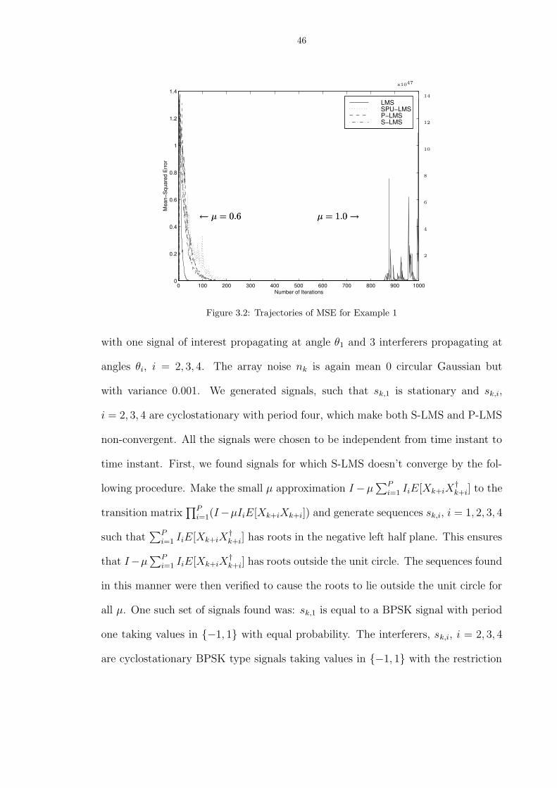
46

0 100 200 300 400 500 600 700 800 900 10000

0.2

0.4

0.6

0.8

1

1.2

1.4

Number of Iterations

Mea

n−S

quar

ed E

rror

LMSSPU−LMSP−LMSS−LMS

x1047

2

4

6

8

10

12

14

µ = 1.0→← µ = 0.6 µ = 1.0→← µ = 0.6

Figure 3.2: Trajectories of MSE for Example 1

with one signal of interest propagating at angle θ1 and 3 interferers propagating at

angles θi, i = 2, 3, 4. The array noise nk is again mean 0 circular Gaussian but

with variance 0.001. We generated signals, such that sk,1 is stationary and sk,i,

i = 2, 3, 4 are cyclostationary with period four, which make both S-LMS and P-LMS

non-convergent. All the signals were chosen to be independent from time instant to

time instant. First, we found signals for which S-LMS doesn’t converge by the fol-

lowing procedure. Make the small µ approximation I −µ∑Pi=1 IiE[Xk+iX

†k+i] to the

transition matrix∏P

i=1(I−µIiE[Xk+iXk+i]) and generate sequences sk,i, i = 1, 2, 3, 4

such that∑P

i=1 IiE[Xk+iX†k+i] has roots in the negative left half plane. This ensures

that I−µ∑Pi=1 IiE[Xk+iX

†k+i] has roots outside the unit circle. The sequences found

in this manner were then verified to cause the roots to lie outside the unit circle for

all µ. One such set of signals found was: sk,1 is equal to a BPSK signal with period

one taking values in −1, 1 with equal probability. The interferers, sk,i, i = 2, 3, 4

are cyclostationary BPSK type signals taking values in −1, 1 with the restriction

47

D=λ/π 4-element Uniform Linear Array

Broadside angle =

Broadside angle =

Broadside angle

−π/4

Cyclostationary BPSK type Interferer, s

s Cyclostationary BPSK type Interferer,

BPSK Signal,s 1,k

3,k

2,k

kd = s k 1,k

1X = A s + A s + A s + n2 2,k k1,k 3 3,k

π/6

=π/4

Figure 3.3: Signal Scenario for Example 2

that sk,2 = 0 if k % 4 6= 1, sk,3 = 0 if k % 4 6= 2 and sk,4 = 0 if k % 4 6= 3. Here a % b

stands for a modulo b. θi, i = 1, 2, 3, 4 are chosen such that θ1 = 1.0388, θ2 = 0.0737,

θ3 = 1.0750 and θ4 = 1.1410. These signals render the S-LMS algorithm unstable

for all µ.

The P-LMS algorithm also fails to converge for the signal set described above

irrespective of µ and the choice of θ1, θ2, θ3, and θ4. Since P-LMS updates the

coefficients every 4th iteration it sees at most one of the three interfering signals

throughout all its updates and hence can place a null at atmost one signal incidence

angle θi. Figure 3.4 shows the envelopes of the e2k trajectories of S-LMS and P-LMS

for the signals given above with the representative value µ = 0.03. As can be seen

P-LMS fails to converge whereas S-LMS shows divergent behavior. SPU-LMS and

LMS were observed to converge for the signal set described above when µ = 0.03.

48

0 1000 2000 3000 4000 5000 6000 70000

10

20

30

40

50

60

70

Number of Iterations

Mea

n S

quar

ed E

rror

P−LMSS−LMS

Figure 3.4: Trajectories of MSE for Example 2

3.8 Examples

3.8.1 I.i.d Gaussian Input Sequence

In this section, we assume that Xk = [xk xk−1 . . . xk−N+1]τ where N is the length

of the vector Xk. xk is a sequence of zero mean i.i.d Gaussian random variables.

We assume that wk = 0 for all k ≥ 0. In that case

Vk+1 = (I − µPkXkX†k)Vk +Xknk V0 = −Wopt,0 = Wopt

where for LMS we have Pk = I and Pk = Ik in case of SPU-LMS. We assume nk is a

white i.i.d. Gaussian noise with variance σ2v . We see that since the conditions (3.13)

and (3.14) are satisfied for theorem 3.2 both LMS and SPU-LMS are exponentially

stable. In fact both have the same α exponent of decay. Therefore, conditions F1

and F2 are satisfied.

We rewrite Vk = J(0)k + J

(1)k + J

(2)k + H

(2)k . Choosing Fk = E[Fk] we have

E[PkXkX†k] = σ2I in the case of LMS and 1

Pσ2I in the case of SPU-LMS. By Theo-

rems 3.3 and 3.4 and Lemmas 3.2 and 3.3 we can upperbound both |J (2)k | and |H

(2)k |

49

by exactly the same constants for LMS and SPU-LMS. In particular, there exists

some constant C <∞ such that for all µ ∈ (0, µ0], we have

supt≥0

∣∣∣E[J

(1)t (J

(2)t +H

(2)t )†]

∣∣∣ ≤ C‖X0‖r(r+δ)/δρ

2r(v)µ

1/2

supt≥0

∣∣∣E[J

(0)t H

(2)t ]∣∣∣ ≤ Cρr(v)‖X0‖r(r+δ)/δµ

1/2.

Next, for LMS we concentrate on

J(0)k+1 = (1− µσ2)J (0)

k +Xknk

J(1)k+1 = (1− µσ2)J (1)

k + µ(σ2I −XkX†k)J

(0)k

and for SPU-LMS we concentrate on

J(0)k+1 = (1− µ

Pσ2)J

(0)k + IkXknk

J(1)k+1 = (1− µ

Pσ2)J

(1)k + µ(

σ2

PI − IkXkX

†k)J

(0)k .

Solving (see Appendix A.6), we obtain for LMS

limk→∞

E[J(0)k (J

(0)k )†] =

σ2vµ(2− µσ2)I

limk→∞

E[J(0)k (J

(1)k )†] = 0

limk→∞

E[J(0)k (J

(2)k )†] = 0

limk→∞

E[J(1)k (J

(1)k )†] =

Nσ2σ2v(2− µσ2)2 I

=Nσ2σ2v

4I +O(µ)I

50

which yields limk→∞E[VkV†k ] =

σ2v

2µI+ Nσ2σ2

v

4I+O(µ1/2)I and for SPU-LMS we obtain

limk→∞

E[J(0)k (J

(0)k )†] =

σ2vµ(2− µ

Pσ2)

I

limk→∞

E[J(0)k (J

(1)k )†] = 0

limk→∞

E[J(0)k (J

(2)k )†] = 0

limk→∞

E[J(1)k (J

(1)k )†] =

(N+1)P−1P

σ2σ2v(2− µ

Pσ2)2

I

=(N+1)P−1

Pσ2σ2v

4I +O(µ)I

which yields limk→∞E[VkV†k ] =

σ2v

2µI +

(N+1)P−1P

σ2σ2v

4I + O(µ1/2)I. Therefore, we see

that SPU-LMS is marginally worse than LMS in terms of misadjustment.

3.8.2 Temporally Correlated Spatially Uncorrelated Array Output

In this section we consider Xk given by

Xk = κXk−1 +√1− κ2Uk

where Uk is a vector of circular Gaussian random variables with unit variance. Similar

to section 3.8.1, we rewrite Vk = J(0)k + J

(1)k + J

(2)k + H

(2)k . Since, we have chosen

Fk = E[Fk] we have E[PkXkX†k] = I in the case of LMS and 1

PI in the case of

SPU-LMS. Again, conditions F1 and F2 are satisfied because of Theorem 3.2. By

[4] and Lemmas 1 and 2 we can upperbound both J(2)k and H

(2)k by exactly the same

constants for LMS and SPU-LMS. By Theorems 3.3 and 3.4 and Lemmas 3.2 and

3.3 we have that there exists some constant C <∞ such that for all µ ∈ (0, µ0], we

have

supt≥0

∣∣∣E[J

(1)t (J

(2)t +H

(2)t )†]

∣∣∣ ≤ C‖X0‖r(r+δ)/δρ

2r(v)µ

1/2

supt≥0

∣∣∣E[J

(0)t H

(2)t ]∣∣∣ ≤ Cρr(v)‖X0‖r(r+δ)/δµ

1/2.

51

Next, for LMS we concentrate on

J(0)k+1 = (1− µ)J (0)

k +Xknk

J(1)k+1 = (1− µ)J (1)

k + µ(I −XkX†k)J

(0)k

and for SPU-LMS we concentrate on

J(0)k+1 = (1− µ

P)J

(0)k + IkXknk

J(1)k+1 = (1− µ

P)J

(1)k + µ(

1

PI − IkXkX

†k)J

(0)k .

Solving (see Appendix A.7), we obtain for LMS

limk→∞

E[J(0)k (J

(0)k )†] =

σ2vµ(2− µ)I

limk→∞

E[J(0)k (J

(1)k )†] = − κ2σ2vN

2(1− κ2)I +O(µ)I

limk→∞

E[J(0)k (J

(2)k )†] =

κ2σ2vN

4(1− κ2)I +O(µ)I

limk→∞

E[J(1)k (J

(1)k )†] =

(1 + κ2)σ2vN

4(1− κ2) I +O(µ)I

which leads to limk→∞E[VkV†k ] =

σ2v

2µI+ Nσ2

v

4I+O(µ1/2)I and for SPU-LMS we obtain

limk→∞

E[J(0)k (J

(0)k )†] =

σ2vµ(2− µ

P)I

limk→∞

E[J(0)k (J

(1)k )†] = − κ2σ2vN

2(1− κ2)P I +O(µ)I

limk→∞

E[J(0)k (J

(2)k )†] =

κ2σ2vN

4(1− κ2)P I +O(µ)I

limk→∞

E[J(1)k (J

(1)k )†] =

σ2v4[N

P

1 + κ2

1− κ2 + (N + 1)P − 1

P]I +O(µ)I

which leads to limk→∞E[VkV†k ] =

σ2v

2µI+ σ2

4[N+1− 1

P]I+O(µ1/2)I. Again, SPU-LMS

is marginally worse than LMS in terms of misadjustment.

3.9 Conclusion and Future Work

We have proposed a new algorithm based on randomization of filter coefficient

subsets for partial updating of filter coefficients. The conditions on step-size for

52

convergence-in-mean and mean-square were shown to be equivalent to those of stan-

dard LMS. It was verified by theory and by simulation that LMS and SPU-LMS

have similar regions of convergence. We also have shown that the Stochastic Partial

Update LMS algorithm has the same performance as the Periodic LMS algorithm

for stationary signals but, can have superior performance for some cyclo-stationary

and deterministic signals.

The idea of random choice of subsets proposed in the chapter can be extended to

include arbitrary subsets of size NP

and not just subsets from a particular partition.

No special advantage is immediately evident from this extension though.

CHAPTER 4

Capacity: Isotropically Random Rician Fading

4.1 Introduction

In this chapter, we analyze MIMO channel capacity under a Rayleigh/Rician fad-

ing model with average energy constraint on the input. The model consists of a line

of sight component (specular component) and a diffuse component (Rayleigh com-

ponent) both changing over time. We model the specular component as isotropically

random statistically independent of the Rayleigh component. This model could ap-

ply to the situation where we have either the transmitter or the receiver in motion

resulting in variable diffuse and specular components.

Traditionally, in a Rician model the fading coefficients are modeled as Gaussian

with non-zero mean. We depart from the traditional model in the sense that we

model the mean (specular component) as time-varying and stochastic. The specular

component is modeled as an isotropic rank one matrix with the specular component

staying constant for T symbol durations and taking independent values every T th

instant. We establish similar properties for this Rician model as those shown by

Marzetta and Hochwald [50] for the Rayleigh fading model. In particular, it is

sufficient to optimize over a smaller parameter set of size minT,M of real valued

magnitudes of the transmitted signals instead of T · M complex valued symbols.

53

54

Furthermore, the capacity achieving signal matrix is shown to be the product of two

independent matrices, a T × T isotropically random unitary matrix and a T ×M

real nonnegative matrix.

The isotropically random Rician fading model is described in detail in section 4.2.

In section 4.4, we derive a new lower bound on capacity. The lower bound also holds

for the case of a purely Rayleigh fading channel. In section 4.5 we show the utility

of this bound by computing capacity regions for both Rayleigh and Rician fading

channels.

4.2 Signal Model

The fading channel is assumed to stay constant for T channel uses and then take

on a completely independent realization for the next T channel uses. Let there be

M transmit antennas and N receive antennas. We transmit a T ×M signal matrix

S and receive a T ×N signal matrix X which are related as follows

X =

√ρ

MSH +W (4.1)

where the elements, wtn of W are independent circularly symmetric complex Gaus-

sian random variables with mean 0 and variance 1 (CN (0, 1)) and ρ is the average

signal to noise ratio present at each of the receive antennas.

The only difference between the Rayleigh model and the Rician model considered

here involves the statistics of the fading matrix H. In the case of the Rayleigh model

the elements hmn of H are modeled as independent CN (0, 1) random variables. For

the isotropically random Rician fading model, the matrix H is modeled as

H =√1− rG+

√rNMvαβ†

where G consists of independent CN (0, 1) random variables, v is a real random

variable such that E[v2] = 1 and α and β are independent isotropically random unit

55

magnitude vectors of lengthM and N , respectively. G, α and β take on independent

values every T th symbol period and remain unchanging in between. The parameter

r ranges between zero and one, with the limits corresponding respectively to purely

Rayleigh or purely specular propagation. Irrespective of the value of r, the average

variance of the components of H is equal to one, E[trHH †] =M ·N .

An M -dimensional unit vector α is isotropically random if its probability density

is invariant to pre-multiplication by an M ×M deterministic unitary matrix, that is

p(Ψα) = p(α), ∀Ψ : Ψ†Ψ = IM [50]. The isotropic density is p(α) = Γ(M)πM

δ(α†α − 1)

where Γ(M) = (M − 1)!.

The choice of the density p(v) of v is not clear. One choice is for p(v) to maximize

the entropy of R = vαβ† corresponding to the worst case scenario (capacity =

minimum) for the channel capacity. One might expect that R corresponding to

maximum entropy would be Gaussian distributed. However, that this is not the case

follows from the proposition below.

Proposition 4.1. There is no distribution p(v) such that the elements of R = vαβ†

have a joint Gaussian distribution, where α and β are isotropically random unitary

vectors, and v, α, and β are mutually independent.

Proof: Proof is by contradiction. Consider the covariance of the elements, Rmn of

R.

E[Rm1n1R∗m2n2

] = E[v2]E[αm1α∗m2

]E[βn1β∗n2]

= E[v2]1

Mδm1m2δn1n2 .

If elements of R were jointly Gaussian then they must be independent of each other

which contradicts the assumption that R is of rank one.

From now on we will assume that v is identically equal to 1. In that case, the

56

conditional probability density function of the measurements at the receiver is given

by

p(X|S) = EαEβ

[

e−tr[IT+(1−r) ρM

SS†]−1(X−√ρrNSαβ†)(X−√ρrNSαβ†)†

πTN detN [IT + (1− r) ρMSS†]

]

where Eα denotes the expectation over the density of α.

Irrespective of whether the fading is Rayleigh or Rician, we have p(Ψ†H) = p(H)

for any M ×M unitary matrix Ψ. In the rest of the section we will deal with H

satisfying this property and refer to Rayleigh and Rician fading as special cases of

this channel. In that case, the condition probability density of the received signals

has the following properties

1. For any T × T unitary matrix Φ

p(ΦX|ΦS) = p(X|S)

2. For any M ×M unitary matrix Ψ

p(X|SΨ) = p(X|S)

Lemma 4.1. If p(X|S) satisfies property 2 defined above then the transmitted signal

can be written as ΦV where Φ is a T × T unitary matrix and V is a T ×M real

nonnegative diagonal matrix.

Proof: Let the input signal matrix S have the SVD ΦVΨ† then the channel can

be written as

X =

√ρ

MΦVΨ†H +W.

Now, consider a new signal S1 formed by multiplying Φ and V and let X1 be the

corresponding received signal. Then

X1 =

√ρ

MΦV H +W.

57

Note that X1 and X have exactly the same statistics since p(Ψ†H) = p(H). There-

fore, one might as well send ΦV instead of ΦVΨ†.

Corollary 4.1. If M > T then power should be transmitted only through T of the

antennas.

Proof: Note that the V in the signal transmitted, ΦV is T ×M . It means that

V = [VT |0] where VT is T × T and 0 is T × (T −M). That means

X =

√ρ

MΦVTHT +W

where HT is the matrix of first T rows in H. That means power is transmitted via

only through T transmit antennas instead of through all M .

Even though the power is transmitted only through the first T transmit antennas

when M > T the capacity corresponding to this case is not the same as the case

when we have M = T antennas. This is one drawback of the model. The model

obtained by starting with T antennas in the first place is not consistent with the

model as starting with M > T antennas and then discarding M − T of them. To

avoid this inconsistency we will assume M ≤ T from now on.

In the case of Rayleigh Fading however there is no such inconsistency and Lemma

4.1 gives rise to a stronger result [50]

Theorem 4.1. For any coherence interval T and any number of receiver antennas,

the capacity obtained with M > T transmitter antennas is the same as the capacity

obtained with M = T antennas.

4.3 Properties of Capacity Achieving Signals

Marzetta and Hochwald [50] have established several results for the case of a

purely Rayleigh fading channel whose proofs were based only on the fact that the

58

conditional probability density satisfies Properties 1 and 2 as stated in section 5.2.

Therefore, the results of [50] are also applicable to the case of the isotropically random

Rician fading channel discussed in this chapter.

Assume the power constraint E[trSS†] ≤ TM .

Lemma 4.2. : Suppose that S has a probability density p0(S) that generates some

mutual information I0. Then, for any M ×M unitary matrix Ψ and for any T × T

unitary matrix Φ, the “rotated” probability density, p1(S) = p0(Φ†SΨ), also generates

I0.

Proof: (For more details refer to the proof for Lemma 1 in [50].) The proof

hinges on the fact that Jacobian determinant of any unitary transformation is one,

p(ΦX|ΦS) = p(X|S), p(X|SΨ†) = p(X|S) and E[trSS†] is invariant to pre- and

post-multiplication of S by unitary matrices.

Lemma 4.3. : For any transmitted signal probability density p0(S), there is a prob-

ability density p1(S) that generates at least as much mutual information and is un-

changed by rearrangements of the rows and columns of S.

Proof: (For more details refer to the proof for Lemma 2 in [50].) From Lemma 4.2

it is evident any density obtained from the original density on S, p0(S) by pre- and

post-multiplying S by any arbitrary permutation matrices PTk, k = 1, . . . , T ! (there

are T ! permutations of the rows) and PMl, l = 1, . . . ,M ! (there are M ! permutations

of the columns), generates the same mutual information. Since mutual information

is a concave functional of the input signal density a mixture input density, p1(S)

formed by taking the average over all densities obtained by permuting S generates

a mutual information at least as large as that of the original density. Note that the

new mixture density satisfies the same power constraint as the original density since

59

E[trSS†] is invariant to permutations of S.

Corollary 4.2. : The following power constraints all yield the same capacity of the

isotropically random Rician fading channel.

• E|stm|2 = 1, m = 1, . . . ,M, t = 1, . . . , T

• 1M

∑Mm=1E|stm|2 = 1, t = 1, . . . , T

• 1T

∑Tt=1E|stm|2 = 1, m = 1, . . . ,M

• 1TM

∑Tt=1

∑Mm=1E|stm|2 = 1

Basically, the corollary tells us that many different types of power constraints

result in the same channel capacity.

Theorem 4.2. The signal matrix that achieves capacity can be written as S = ΦV ,

where Φ is a T × T isotropically distributed unitary matrix, and V is an indepen-

dent T × M real, nonnegative, diagonal matrix. Furthermore, we can choose the

joint density of the diagonal elements of V to be unchanged by rearrangements of its

arguments.

Proof: Proof is similar to the proof for Theorem 2 in [50].

4.4 Capacity Upper and Lower Bounds

First we will state the following result which has already been established in [50],

and follows in a straightforward manner from [73].

Theorem 4.3. The expression for capacity of the isotropically random Rician fading

channel when only the receiver has complete knowledge about the channel (informed

receiver uninformed transmitter) is

CH = T · E log det[

IN +ρ

MH†H

]

.

60

The following general upper bound on capacity is quite intuitive [10, 50].

Proposition 4.2. An upper bound on capacity of the isotropically random Rician

fading channel when neither the transmitter nor the receiver has any knowledge about

the channel (uninformed receiver uninformed transmitter) is given by

C ≤ CH = T · E log det[

IN +ρ

MH†H

]

. (4.2)

What is lacking is a tractable lower bound on capacity of the isotropically random

Rician fading channel. In this work we establish such a lower bound when no channel

information is present at either the transmitter or the receiver.

Theorem 4.4. A lower bound on capacity of the isotropically random Rician fading

channel when neither the transmitter nor the receiver has any knowledge about the

channel is given by

C ≥ TE[

log2 det(

IN +ρ

MH†H

)]

−NE[

log2 det(

IT +ρ

MSS†

)]

(4.3)

≥ TE[

log2 det(

IN +ρ

MH†H

)]

−NM log2(1 +ρ

MT ). (4.4)

Proof: First note that the capacity C is given by

C = maxp(S)

[I(X;S) = H(X)−H(X|S)]

by choosing a specific distribution on S, in this case CN (0, 1), we get a lower bound

to C. Note that H(X|H) ≤ H(X) so that we obtain

C ≥ H(X|H)−H(X|S). (4.5)

Since p(S) = 1πTM

exp(−trSS†

)(the elements of S are CN (0, 1) random vari-

ables)

H(X|H) = TE[

log2

(

(πe)N det(

IN +ρ

MH†H

))]

.

61

Now we turn to evaluating H(X|S). Note that since p(Ψ†H) = p(H) for all unitary

matrices Ψ, E[hm1n1h∗m2n2

] = δm1m2δn1n2 . Therefore given S, X has covariance given

by

E[xt1n1x∗t2n2|S] = δn1n2 ·

[

δt1t2 +ρ

M

M∑

m=1

st1ms∗t2m

]

.

Since H(X|S) is bounded above by the entropy HG(X|S) of a Gaussian with the

same mean and covariance as X given S we have

HG(X|S) ≤ NE[

log2

(

(πe)T det(

IT +ρ

MSS†

))]

where the expectation is over the distribution of S which gives us (4.3).

Next we simplify the expression above further to obtain a looser lower bound. We

use the property that for any T ×M matrix S, det(IT +SS†) = det(IM +S†S). This,

along with the fact that log2 det(K) is convex cap and Jensen’s inequality, gives

NE[

log2 det(

IT +ρ

MSS†

)]

≤ N log2 det(

IM +ρ

ME[S†S]

)

(4.6)

= NM log2(1 +ρ

MT ). (4.7)

Therefore, we obtain (4.4).

Note that the expression on the right hand side in (4.5) can be rewritten as

I(X;S|H) − I(X;H|S). I(X;S|H) is the mutual information when H is known to

the receiver and I(X;H|S) is the information contained in X about H when S is

known at the receiver and therefore, I(X;H|S) can be viewed as the penalty for

learning H in the course of decoding S from the reception of X.

A simple improved lower bound in either (4.3) or (4.4) can be obtained by opti-

mizing over the number of transmit and receive antennas used. Note that both the

expressions in the right hand side of (4.3) can be easily evaluated using Monte Carlo

simulations.

62

From the lower bound (4.4) it can be easily seen that as T →∞ the normalized

capacity, Cn = C/T in bits per channel use is given by that of the informed receiver

Cn = E log det[

IN +ρ

MH†H

]

.

This was conjectured for the Rayleigh fading channel by Marzetta and Hochwald in

[50] and discussed in [10, p. 2632].

4.5 Numerical Results

First we show the utility of the lower bound by comparing it with the actual

capacity curve calculated in [50] for the case of a single transmit and receive antennas

in a purely Rayleigh fading environment for increasing T . We plot the upper bound

(4.2), the lower bound derived (4.3) and the actual capacity obtained in [50] from

numerical integration in Figure 4.1. The utility of this bound is clearly evident from

how well the lower bound follows the actual capacity.

5 10 15 20 25 30 35 400

0.1

0.2

0.3

0.4

0.5

0.6

0.7

0.8

0.9

1

T (Coherence Interval)

Cap

acity

(bits

/T)

Capacity Upper Bound

Capacity Lower Bound

Actual Capacity

(a) ρ = 0dB

5 10 15 20 25 30 350

0.5

1

1.5

2

2.5

3

3.5

4

T (Coherence Interval)

Cap

acity

(bits

/T)

Capacity Upper Bound

Capacity Lower Bound

Actual Capacity

(b) ρ = 12dB

Figure 4.1: Capacity and Capacity lower bound for M = N = 1 as T →∞

In different simulations, using the upper and lower bounds, we found that the

capacity variation as a function of r, i.e. as the channel moves from a purely Rayleigh

63

(r = 0) to a purely specular channel (r = 1)become more pronounced as we move to

higher SNR regimes and larger number of transmit and receive antennas, M and N

respectively. Examples of this behavior are shown in Figures 4.2 and 4.3. Note that

for the special case of M = N = 1 the capacity curves have an upward trend as r

varies from 0 to 1. For all other cases the capacity curves have a downward trend,

where the reduction in capacity becomes significant only for r > 1/2.

0 0.1 0.2 0.3 0.4 0.5 0.6 0.7 0.8 0.9 10

1

2

3

4

5

6

7

8

9M = N = 2

r (fraction of power in Rician component)

Cap

acity

(bits

/T)

Upper Bound, T = 4, 8, 16

Lower Bound, T = 16

Lower Bound, T = 8

Lower Bound, T = 4

(a) ρ = 0dB

0 0.1 0.2 0.3 0.4 0.5 0.6 0.7 0.8 0.9 10

1

2

3

4

5

6

7

8

9M = N = 2

r (fraction of power in Rician component)

Cap

acity

(bits

/T)

Upper Bound, T = 4, 8, 16

Lower Bound, T = 16

Lower Bound, T = 8

Lower Bound, T = 4

(b) ρ = 15dB

Figure 4.2: Capacity upper and lower bounds as the channel moves from purely Rayleigh to purelyRician fading

4.6 Analysis for High SNR

The techniques developed in [85] can be easily applied to the model in this section

to conclude that the number of degrees of freedom is given by M ∗(T −M ∗) where

M∗ = minM,N, T/2. All the Theorems developed in [85] can be easily translated

to the case of isotropically random Rician fading.

We will now investigate whether the lower bound derived in this chapter attains

the required number of degrees of freedom. We will compare this lower bound with

the capacity expression derived in [85] for high SNR. Figure 4.4 shows the actual

64

0 0.2 0.4 0.6 0.8 10

2

4

6

8

10

12

14

16

18

20N = 4

r (fraction of power in Rician component)

Cap

acity

(bits

/T)

T = 2, M = 1 T = 4, M = 2 T = 8, M = 4

(a) ρ = 0dB

0 0.2 0.4 0.6 0.8 10

2

4

6

8

10

12

14

16

18

20N = 4

r (fraction of power in Rician component)

Cap

acity

(bits

/T)

T = 2, M = 1 T = 4, M = 2 T = 8, M = 4

(b) ρ = 15dB

Figure 4.3: Capacity upper and lower bounds as the channel moves from purely Rayleigh to purelyRician fading

capacity and the lower bound as a function of increasing SNR for a purely Rayleigh

fading channel. In both cases T > M ∗ + N where M ∗ = minM,N, T/2 as the

actual capacity expression is not known for T < M ∗ + N [85]. As can be seen this

lower bound attains the required number of degrees of freedom.

0 50 100 150−50

0

50

100

150

200

250M = N = 5, T = 50

SNR (dB)

Cap

acity

(bits

/T)

Capacity lower bound

Capacity

(a) M = N = 5, T = 50

0 50 100 1500

10

20

30

40

50

60

70M = 4, N = 2, T = 6

SNR (dB)

Cap

acity

(bits

/T)

Capacity

Capacity lower bound

(b) M = 4, N = 2, T = 6

Figure 4.4: Capacity and capacity lower bound as a function of SNR for a purely Rayleigh fadingchannel

65

4.7 Conclusions

We have analyzed the case of isotropically random Rician fading channel. We

have proposed a tractable model for Rician fading with a stochastic isotropic specular

component of rank one. Using this model we were able to establish most of the results

previously obtained in the case of Rayleigh fading. We were also able to derive a

lower bound on capacity for any number of transmit and receive antennas. This

lower bound is also applicable to the case of Rayleigh fading. For single transmit

and receive antennas, the Rician channel gives superior performance with respect

to the Rayleigh channel. For multiple antenna channels, Rician fading tends to

degrade the performance. Our numerical results indicate that the Rayleigh model is

surprisingly robust: under our Rician model, up to half of the received energy can

arrive via the specular component without significant reduction in capacity compared

with the purely Rayleigh case. Finally, the model considered in this chapter has a

drawback as explained after Lemma 4.1. Inspite of the drawback the model is helpful

in understanding the Rician channel.

CHAPTER 5

Min-Capacity: Rician Fading, Unknown Static SpecularComponent

5.1 Introduction

In the previous chapter we considered an isotropic model for the case of Rician

fading where the fading channel consists of a Rayleigh component, modeled as in

[50] and an independent rank-one isotropically distributed specular component. The

fading channel was assumed to remain constant over a block of T consecutive symbol

periods but take a completely independent realization over each block. We derived

similar results on optimal capacity achieving signal structures as in [50]. We also

established a lower bound to capacity that can be easily extended to the model

considered in this chapter. The model described in the previous chapter is applicable

to a mobile-wireless link where both the direct line of sight component (specular

component) and the diffuse component (Rayleigh component) change with time.

In this chapter, we consider MIMO channel capacity, under the average energy

constraint on the input signal, of a quasi-static Rician model where the specular

component is non-changing while the Rayleigh component is varying over time. This

model is similar to the traditional model where the specular component is determinis-

tic and persists over time. The model is applicable to the case where the transmitter

and receiver are fixed in space, are in motion, or the propagation medium is changing

66

67

where the transmitter and the receiver are sufficiently far apart so that the specular

component is practically constant while the diffuse multipath component changes

rapidly. If the specular component were known to both the transmitter and the re-

ceiver then the signaling scheme as well as the capacity would depend on the specific

realization of the specular component. We however deal with the case when the

transmitter has no knowledge about the specular component. In this scenario the

transmitter has to treat the specular component as a random variable with a prior

distribution. There are two approaches the transmitter can take. It can either ignore

the distribution, treat the channel as an arbitrarily varying channel and maximize

the worst case rate over the ensemble of values that the specular component can take

on or take into account the prior distribution of the specular component and then

maximize the average rate. We address both approaches in this chapter.

Similarly to [21] the specular component is an outer product of two vectors of

unit magnitude that are non-changing and unknown to the transmitter but known

to the receiver. The difference between our approach and that of [21] is that in

[21] the authors consider the channel to be known completely to the receiver. We

assume that the receiver’s extent of knowledge about the channel is limited to the

specular component. That is, the receiver has no knowledge about the Rayleigh

component of the model. Considering the absence of knowledge at the transmitter

it is important to design a signal scheme that guarantees the largest overall rate

for communication irrespective of the value of the specular component. This is

formulated as the problem of determining the worst case capacity called min-capacity,

in section 5.2. In section 5.5 we consider the average capacity instead of worst case

capacity and show that both formulations imply the same optimal signal structure

and the same maximum possible rate. Throughout this chapter we assume that the

68

transmitter has no knowledge about the channel though it has knowledge of the

statistics of the Rayleigh component of the channel. Only in 5.5 do we assume that

the channel has knowledge of the statistics of the specular component as well.

5.2 Signal Model and Min-Capacity Criterion

Let there be M transmit antennas and N receive antennas. We assume that the

fading coefficients remain constant over a block of T consecutive symbol periods but

are independent from block to block. Keeping that in mind, we model the channel

as carrying a T ×M signal matrix S over a M ×N MIMO channel H, producing X

at the receiver according to the model:

X =

√ρ

MSH +W (5.1)

where the elements, wtn of W are independent circular complex Gaussian random

variables with mean 0 and variance 1 (CN (0, 1)).

The MIMO Rician model for the matrix H is H =√1− rG+

√rNMαβ† where

G consists of independent CN (0, 1) random variables and α and β are deterministic

vectors of lengthM and N , respectively, such that α†α = 1 and β†β = 1. We assume

α and β are known to the receiver. Since the receiver is free to apply a co-ordinate

transformation by post multiplying X by a unitary matrix, without loss of generality

we can take β to be identically equal to [1 0 . . . 0]τ . We will sometimes write H as

Hα to highlight the dependence of H on α. G remains constant for T symbol periods

and takes on a completely independent realization every T th symbol period.

The problem we are investigating is to find the distribution pm(S) that attains the

maximum in the following maximization defining the worst case channel capacity

Cm = maxp(S)

Im(X;S) = maxp(S)

infα∈A

Iα(X;S)

69

and also to find the maximum value, Cm.

Iα(X;S) =

∫

p(S)p(X|S, αβ†) log p(X|S, αβ†)∫p(S)p(X|S, αβ†) dS dSdX

is the mutual information between X and S when the specular component is given

by αβ† and Adef= α : α ∈ Cl M and α†α = 1. Note that since β = [1 0 . . . 0]τ

without any loss of generality we can write p(X|S, αβ†) as simply p(X|S, α) and is

given by

p(X|S, α) = e−tr[IT+(1−r) ρM

SS†]−1(X−√ρrNSαβ†)(X−√ρrNSαβ†)†

πTN detN [IT + (1− r) ρMSS†]

.

Since A is compact the “inf” in the problem can be replaced by “min”. For con-

venience we will refer to Im(X;S) as the min-mutual information and Cm as min-

capacity.

The min-capacity defined above is just the capacity of a compound channel. For

more information on the concept of compound channels, worst case capacities and the

corresponding coding theorems refer to [14, chapter 5, pp. 172-178]. It is shown that

[14, Prob. 13, p. 183] min-capacity doesn’t depend on the receiver’s knowledge of

the channel. Hence, it is not necessary for us to assume that the specular component

is known to the receiver. However, we do so because it facilitates computation of

avg-capacity in terms of the conditional probability distribution p(X|S).

5.3 Capacity Upper and Lower Bounds

Theorem 5.1. Min-capacity, CmH of the quasi-static Rician fading model when the

channel matrix H is known to the receiver is given by

CmH = TE log det

[

IN +ρ

MH†

e1He1

]

(5.2)

where e1 = [1 0 . . . 0]τ is a unit vector in Cl M . Note that e1 in (5.2) can be replaced

by any α ∈ A without changing the answer.

70

Proof: First we note that for T > 1, given H the channel is memoryless and

hence the columns of the input signal matrix S are independent of each other. That

means the mutual information Iα(X;S) =∑T

i=1 Iα(Xi;Si) where Xi and Si denote

the ith row of X and S, respectively. The maximization over each term can be done

separately and it is easily seen that each term will be maximized individually for

the same density on Si. That is p(Si) = p(Sj) for i 6= j and maxp(S) Iα(X;S) =

T maxp(S1) Iα(X1;S1). Therefore, WLOG we assume T = 1.

Given H the channel is an AWGN channel therefore, capacity is attained by

Gaussian signal vectors. Let ΛS be the input signal covariance. Since the transmitter

doesn’t know α, ΛS can not depend on α and the min-capacity is given by

maxΛS :trΛS≤M

F(ΛS) = maxΛS :trΛS≤M

minα∈A

E log det[

IN +ρ

MH†

αΛSHα

]

(5.3)

where F(ΛS) is implicitly defined in an obvious manner. First note that F(ΛS) in

(5.3) is a concave function of ΛS (This follows from the fact that log detK is a concave

function of K). Also, F(Ψ†ΛSΨ) = F(ΛS) for any M ×M Ψ : Ψ†Ψ = IM since

Ψ†α ∈ A for any α ∈ A and G has i.i.d. zero mean complex Gaussian entries. Let

Q†DQ be the SVD of ΛS then we have F(D) = F(Q†DQ) = F(ΛS). Therefore, we

can choose ΛS to be diagonal. Moreover, F(P †kΛSPk) = F(ΛS) for any permutation

matrix Pk, k = 1, . . . ,M !. Therefore, if we choose Λ′S = 1M !

∑M !k=1 P

†kΛSPk then by

concavity and Jensen’s inequality we have

F(Λ′S) ≥M !∑

k=1

F(P †kΛSPk) = F(ΛS).

Therefore, we conclude that the maximizing input signal covariance ΛS is a multiple

of the identity matrix. To maximize the expression in (5.3) we need to choose

trΛS = M or ΛS = IM and since E log det[IN + ρMH†

α1Hα1 ] = E log det[IN +

ρMH†

α2Hα2 ] for any α1, α2 ∈ A, (5.2) easily follows.

71

By the data processing theorem additional information at the receiver doesn’t

decrease capacity. Therefore:

Proposition 5.1. An upper bound on the channel min-capacity of the quasi-static

Rician fading channel when the receiver has no knowledge of G is given by

Cm ≤ T · E log det[

IN +ρ

MH†

e1He1

]

. (5.4)

Now, we establish a lower bound.

Proposition 5.2. A lower bound on min-capacity of the quasi-static Rician fading

channel when the the receiver has no knowledge about G is given by

Cm ≥ CmH −NE

[

log2 det(

IT + (1− r) ρMSS†

)]

(5.5)

≥ CmH −NM log2(1 + (1− r) ρ

MT ). (5.6)

Proof: Proof is similar to that of Theorem 4.4 and won’t be repeated here.

Notice that the second term in right hand side of the lower bound is

NE[

log2 det(

IT + (1− r) ρMSS†

)]

instead of NE[log2 det

(IT + ρ

MSS†

)]which occurs in the lower bound derived for

the model in the previous chapter. Recall that we have seen how the second term

can be viewed as a penalty term for using part of the available rate for training in

order to learn the channel. When r = 1 or when the channel is purely specular we

see that the penalty term for training goes to zero. This makes perfect sense because

the specular component is known to the receiver and the penalty for learning the

specular component is zero in the current model as contrasted to the model in the

previous chapter.

Combining (5.4) and (4.4) gives us the following

72

Corollary 5.1. The normalized min-capacity, Cmn = Cm/T in bits per channel use as

T →∞ of the quasi-static Rician fading channel when the receiver has no knowledge

of G is given by

Cmn = E log det

[

IN +ρ

MH†

e1He1

]

.

Note that this is same as the capacity when the receiver knows H, so that as

T →∞ perfect channel estimation can be performed.

5.4 Properties of Capacity Achieving Signals

In this section, we derive the optimum signal structure for achieving min-capacity.

The optimization is done under the average power constraint E[trSS†] ≤ TM .

Lemma 5.1. Im(X;S), for the quasi-static Rician fading channel when the receiver

has no knowledge of G, as a functional of p(S) is concave in p(S).

Proof: First we note that Iα(X;S) is a concave functional of p(S) for every α ∈ A.

Let Im(X;S)p(S) denote Im(X;S) evaluated using p(S) as the signal density. Then,

Im(X;S)δp1(S)+(1−δ)p2(S) = minα∈A

Iα(X;S)δp1(S)+(1−δ)p2(S)

≥ minα∈A

[δIα(X;S)p1(S) + (1− δ)Iα(X;S)p2(S)]

≥ δminα∈A

Iα(X;S)p1(S) + (1− δ)minα∈A

Iα(X;S)p2(S)

= δIm(X;S)p1(S) + (1− δ)Im(X;S)p2(S).

Lemma 5.2. For any T ×T unitary matrix Φ and any M ×M unitary matrix Ψ, if

p(S) generates Im(X;S) then so does p(ΦSΨ†) when the fading is quasi-static Rician

fading and the receiver has no knowledge of the Rayleigh component.

73

Proof: 1) Note that p(ΦX|ΦS) = p(X|S), therefore Iα(X; ΦS) = Iα(X;S) for

any T × T unitary matrix Φ and all α ∈ A.

2) We have, Ψα ∈ A for any α ∈ A and any M ×M unitary matrix Ψ. Therefore,

if Im(X;S) achieves its minimum value at α0 ∈ A then Im(X;SΨ†) achieves its

minimum value at Ψα0 because Iα(X;S) = IΨα(X;SΨ†) for α ∈ A and Ψ anM×M

unitary matrix.

Combining 1) and 2) we get the lemma.

Lemma 5.3. The min-capacity achieving signal distribution, p(S) when G is not

known at the receiver for the quasi-static Rician fading channel is unchanged by any

pre- and post- multiplication of S by unitary matrices of appropriate dimensions.

Proof: We will show that for any signal density p0(S) generating min-mutual

information Im0 there exists a density p1(S) generating Im1 ≥ Im0 such that p1(S) is

invariant to pre- and post- multiplication of S by unitary matrices of appropriate

dimensions. By Lemma 5.2, for any pair of permutation matrices, Φ (T × T ) and

Ψ (M ×M) p0(ΦSΨ†) generates the same min-mutual information as p(S). Define

uT (Φ) to be the isotropically random unitary density function of a T × T unitary

matrix Φ. Similarly define uM(Ψ). Let p1(S) be a mixture density given as follows

p1(S) =

∫ ∫

p0(ΦSΨ†)u(Φ)u(Ψ) dΦdΨ.

It is easy to see that p1(S) is invariant to any pre- and post- multiplication of S by

unitary matrices and if Im1 is the min-mutual information generated by p1(S) then

from Jensen’s inequality and concavity of Im(X;S) we have Im1 ≥ Im0 .

Corollary 5.2. pm(S), the optimal min-capacity achieving signal density, for the

quasi-static Rician fading channel when the receiver has no knowledge of G, lies in

74

P = ∪I>0PI where

PI = p(S) : Iα(X;S) = I ∀α ∈ A. (5.7)

Proof: Follows immediately from Lemma 5.3 because any signal density that is

invariant to pre- and post- multiplication of S by unitary matrices generates the

same mutual information Iα(X;S) irrespective of the value of α.

Corollary 5.3. The min-capacity achieving signal distribution p(S) for the quasi

static Rician fading channel when the receiver does not know G is unchanged by

rearrangements of elements in S.

Corollary 5.4. : The following power constraints all yield the same channel min-

capacity of the quasi-static Rician fading channel when the receiver does not know

G.

• E|stm|2 = 1, m = 1, . . . ,M, t = 1, . . . , T

• 1M

∑Mm=1E|stm|2 = 1, t = 1, . . . , T

• 1T

∑Tt=1E|stm|2 = 1, m = 1, . . . ,M

• 1TM

∑Tt=1

∑Mm=1E|stm|2 = 1

Theorem 5.2. The signal matrix that achieves min-capacity, for the quasi-static

Rician fading channel when the Rayleigh component is not known at the receiver,

can be written as S = ΦVΨ†, where Φ and Ψ are T × T and M ×M isotropically

distributed matrices independent of each other, and V is a T ×M real, nonnegative,

diagonal matrix, independent of both Φ and Ψ.

Proof: From the singular value decomposition (SVD) we can write S = ΦVΨ†,

where Φ is a T × T unitary matrix, V is a T ×M nonnegative real diagonal matrix,

75

and Ψ is an M ×M unitary matrix. In general, Φ, V and Ψ are jointly distributed.

Suppose S has probability density p0(S) that generates min-mutual information Im0 .

Let Θ1 and Θ2 be isotropically distributed unitary matrices of size T ×T andM×M

independent of S and of each other. Define a new signal S1 = Θ1SΘ†2, generatingmin-

mutual information Im1 . Now conditioned on Θ1 and Θ2, the min-mutual information

generated by S1 equals Im0 . From the concavity of the min-mutual information as a

functional of p(S), and Jensen’s inequality we conclude that Im1 ≥ Im0 .

Since Θ1 and Θ2 are isotropically distributed Θ1Φ and Θ2Ψ are also isotropically

distributed when conditioned on Φ and Ψ respectively. This means that both Θ1Φ

and Θ2Ψ are isotropically distributed making them independent of Φ, V and Ψ.

Therefore, S1 is equal to the product of three independent matrices, a T ×T unitary

matrix Φ, a T ×M real nonnegative matrix V and an M ×M unitary matrix Ψ.

Now, we will show that the density p(V ) on V is unchanged by rearrangements of

diagonal entries of V . There are minM !, T ! ways of arranging the diagonal entries

of V . This can be accomplished by pre- and post-multiplying V by appropriate

permutation matrices, PTk and PMk, k = 1, . . . ,minM !, T !. The permutation does

not change the min-mutual information because ΦPTk and ΨPMk have the same

density functions as Φ and Ψ. By choosing an equally weighted mixture density

for V , involving all minM !, T ! arrangements we obtain a higher value of min-

mutual information because of concavity and Jensen’s inequality. This new density

is invariant to the rearrangements of the diagonal elements of V .

5.5 Average Capacity Criterion

In this case we maximize IE(X;S) = Eα[Iα(X;S)], where Iα is as defined earlier

and Eα denotes expectation over α ∈ A under the assumption that all α are equally

76

likely. That is, under the assumption that α is unchanging over time, isotropically

random and known to the receiver. Please note that this differs from the model

considered in Chapter 4 where we consider the case of a piecewise constant, time

varying, i.i.d. specular component.

Therefore, the problem can be stated as finding pE(S) the probability density

function on the input signal S that achieves the following maximization

CE = maxp(S)

Eα[Iα(X;S)] (5.8)

and also to find the value CE. We will refer to IE(X;S) as avg-mutual information

and CE as avg-capacity.

We will show that the signal density pm(S) that attains Cm also attains CE. For

this we need to establish the following Lemmas.

Lemma 5.4. IE(X;S) for the quasi-static Rician fading channel is a concave func-

tion of the signal density p(S) when the receiver does not know G and the transmitter

takes into account the statistics of the specular component.

Proof: First we note that Iα(X;S) is a concave functional of p(S) for every α ∈ A.

Then,

IE(X;S)δp1(S)+(1−δ)p2(S) = Eα[Iα(X;S)δp1(S)+(1−δ)p2(S)]

≥ Eα[δIα(X;S)p1(S) + (1− δ)Iα(X;S)p2(S)]

= δEα[Iα(X;S)p1(S)] + (1− δ)Eα[I

α(X;S)p2(S)]

= δIE(X;S)p1(S) + (1− δ)IE(X;S)p2(S).

Lemma 5.5. For any T × T unitary matrix Φ and any M ×M unitary matrix Ψ,

if p(S) generates IE(X;S) then so does p(ΦSΨ†) when the fading is quasi-static, the

77

receiver does not know G and the transmitter takes into account the statistics of the

specular component.

Proof: We want to show if p(S) generates IE(X;S) then so does p(ΦSΨ†). Now

since the density function of α, p(α) = Γ(M)πM

δ(α†α− 1) we have

IE(X;S) =πM

Γ(M)

∫

Iα(X;S) dα.

Note that Iα(X; ΦS) = Iα(X;S) and IΨα(X;SΨ†) = Iα(X;S) ⇒ IΨ†α(X;S) =

Iα(X;SΨ†). Therefore,

I ′E(X;S) =πM

Γ(M)

∫

Iα(X; ΦSΨ†) dα

=πM

Γ(M)

∫

Iα(X;SΨ†) dα

=πM

Γ(M)

∫

IΨ†α(X;S) dα

=πM

Γ(M)

∫

Iω(X;S) dω

= IE(X;S)

where the last two equalities follow from the transformation ω = Ψ†α and the fact

the Jacobian of the transformation is equal to 1.

Lemma 5.6. The avg-capacity achieving signal distribution, p(S) is unchanged by

any pre- and post- multiplication of S by unitary matrices of appropriate dimensions

when the fading is quasi-static, the receiver does not know G and the transmitter

takes into account the statistics of the specular component.

Corollary 5.5. pE(S), the optimal avg-capacity achieving signal density lies in

P = ∪I>0PI where PI is as defined in (5.7) when the fading is quasi-static Rician

fading, the receiver has no knowledge of G and the transmitter takes into account the

statistics of the specular component.

78

Based on the last corollary we conclude that for a given p(S) in P we have

Im(X;S) = minα∈A Iα(X;S) = Eα[Iα(X;S)] = IE(X;S). Therefore, the maximiz-

ing densities for CE and Cm are the same and also CE = Cm. Therefore, designing

the signal constellation with the objective of maximizing the worst case performance

is not more pessimistic than maximizing the average performance.

5.6 Coding Theorem for Min-capacity

In this section, we will prove the following theorem.

Theorem 5.3. For the quasi-static Rician fading model, for every R < Cm there

exists a sequence of (2nR, n) codes with codewords, mni , i = 1, . . . , 2nR, satisfying the

power constraint such that

limn→∞

supαPeα,n = 0

where Peα,n = max2nR

i=1 Pe(mni , α) and Pe(mi) is the probability of incorrectly decoding

the messages mi when the channel is given by Hα.

Proof: Proof follows if we can show that Peα,n is bounded above by the same

Gallager error exponent [26, 27] irrespective of the value of α. That follows from the

following lemma (Lemma 5.7).

The intuition behind the existence of a coding theorem is that the min-capacity

Cm, is the mutual information between the output and the input for some particular

channel Hα (Since A = α : α ∈ Cl M and α†α = 1 is compact). Therefore, any

codes generated from the random coding argument designed to achieve rates up to

Cm for that particular Hα achieve rates up to Cm for all Hα.

For Lemma 5.7, we first need to briefly describe the Gallager error exponents

[26, 27] for the quasi-static Rician fading channel. For a system communicating at a

79

rate R the upper bound on the maximum probability of error is given as follows

Peα,n ≤ exp

(

−nmaxp(S)

max0≤γ≤1

[E0(γ, p(S), α)− γR log 2]

)

where n is the length of the codewords in the codebook used and E0(γ, p(S), α) is as

follows

E0(γ, p(S), α) = − log

∫ [∫

p(S)p(X|S, α) 11+γ dS

]γ

dX

where S is the input to the channel and X is the observed output and

p(X|S, α) = e−tr[IT+(1−r) ρM

SS†]−1(X−√ρrNSαβ†)(X−√ρrNSαβ†)†

πTN detN [IT + (1− r) ρMSS†]

.

where β is simply [1 0 . . . 0]τ . Maximization over γ in the error exponent yields a

value of γ such that ∂E0(γ,p(S),α)∂γ

= R. Note that for γ = 0, ∂E0(γ,p(S),α)∂γ

= Iα(X;S)

[26, 27] where the mutual information has been evaluated when the input is p(S). If

p(S) is the min-capacity achieving density, pm(S) then ∂E0(γ,pm(S),α)∂γ

= Cm. For more

information refer to [26, 27].

Lemma 5.7. The E0(γ, pm(S), α) for the quasi-static Rician fading model is inde-

pendent of α.

Proof: First, note that

pm(S) = pm(S؆)

for any M ×M unitary matrix Ψ. Second,

E0(γ, pm(S), α) = − log

∫ [∫

pm(S)p(X|S, α) 11+γ dS

]γ

dX

= − log

∫ [∫

pm(SΨ†)p(X|SΨ†, α) 11+γ dS

]γ

dX

= − log

∫ [∫

pm(S)p(X|S,Ψ†α) 11+γ dS

]γ

dX

= E0(γ, pm(S),Ψ†α)

80

where the second equation follows from the fact that Ψ is a unitary matrix and its Ja-

cobian is equal to 1 and the third equation follows from the fact that p(X|SΨ†, α) 11+γ =

p(X|S,Ψ†α) 11+γ . Since Ψ is arbitrary we obtain that E0(γ, p

m(S), α) is independent

of α.

5.7 Numerical Results

Plotting the capacity upper and lower bounds leads to similar conclusions as in

the previous chapter except for the fact when r = 1 the upper and lower bounds on

capacity coincide.

In Figure 5.1 we plot the capacity and upper lower bounds as a function of the

Rician parameter r. We see that the change in capacity is not drastic for low SNR as

compared to larger SNR values. Also, from Figure 5.2 we conclude that this change in

capacity is more prominent for larger number of antennas. We also conclude that for

a purely specular channel increasing the number of transmit antennas has no effect

on the capacity. This is due to the fact that with a rank-one specular component,

only beamforming SNR gains can be exploited, no diversity gains are possible.

5.8 Conclusions

We have proposed another tractable model for Rician fading channel different

from the one in Chapter 4 but, along the lines of [21]. We were able to analyze this

channel and derive some interesting results on optimal signal structure. We were also

able to show that the optimization effort is over a much smaller set of parameters

than the set originally started with. We were also able to derive a lower bound that

is useful since the capacity is not in closed form.

Finally, we were able to show that the approach of maximizing the worst case

scenario is not overly pessimistic in the sense that the signal density maximizing the

81

0 0.1 0.2 0.3 0.4 0.5 0.6 0.7 0.8 0.9 10

1

2

3

4

5

6

7

8

9M = N = 4

r

Cap

acity

(bits

/T)

Upper bound, T = 4, 8, 16

Lower bound, T = 4

Lower bound, T = 16

Lower bound, T = 8

(a) ρ = 0dB

0 0.1 0.2 0.3 0.4 0.5 0.6 0.7 0.8 0.9 12

4

6

8

10

12

14

16

18M = N = 4

r

Cap

acity

(bits

/T)

Upper bound, T = 4, 8, 16

Lower bound, T = 4

Lower bound, T = 16

Lower bound, T = 8

(b) ρ = 15dB

Figure 5.1: Capacity upper and lower bounds as the channel moves from purely Rayleigh to purelyRician fading

0 0.1 0.2 0.3 0.4 0.5 0.6 0.7 0.8 0.9 10

2

4

6

8

10

12

14

16

18

20N = 4

r

Cap

acity

(bits

/T)

T = 2, M = 1 T = 4, M = 2 T = 8, M = 4

(a) ρ = 0dB

0 0.1 0.2 0.3 0.4 0.5 0.6 0.7 0.8 0.9 10

2

4

6

8

10

12

14

16

18

20N = 4

r

Cap

acity

(bits

/T)

T = 2, M = 1 T = 4, M = 2 T = 8, M = 4

(b) ρ = 15dB

Figure 5.2: Capacity upper and lower bounds as the channel moves from purely Rayleigh to purelyRician fading

82

worst case performance also maximizes the average performance and the capacity

value in both formulations turns out to be the same. The average capacity being

equal to the worst case capacity can also be interpreted in a different manner: we

have shown that the average capacity criterion is a quality of service guaranteeing

capacity.

CHAPTER 6

Capacity: Rician Fading, Known Static Specular Component

6.1 Introduction

In Chapter 4, we considered a model where the specular component is rank-one

and has an isotropic distribution. In Chapter 5, we considered a model where the

specular component is deterministic and static but unknown to the transmitter. Both

these models led to a tractable analysis of the capacity or min-capacity of the Rician

fading model. Also, the specular component considered in both the chapters was

of rank one. Here we consider the Rician fading model with a fixed deterministic

specular fading component.

In this chapter, we analyze the standard Rician fading model for capacity un-

der the average energy constraint on the input signal. Throughout the chapter, we

assume that the specular component is deterministic and is known to both the trans-

mitter and the receiver. The specular component in this chapter is of general rank

except in section 6.2 where it is restricted to be of rank one. Throughout this chapter

the Rayleigh component is never known to the transmitter. There are some cases we

consider where the receiver has complete knowledge of the channel. In such cases,

the receiver has knowledge about the Rayleigh as well as the specular component

whereas the transmitter has knowledge only about the specular component. The ca-

83

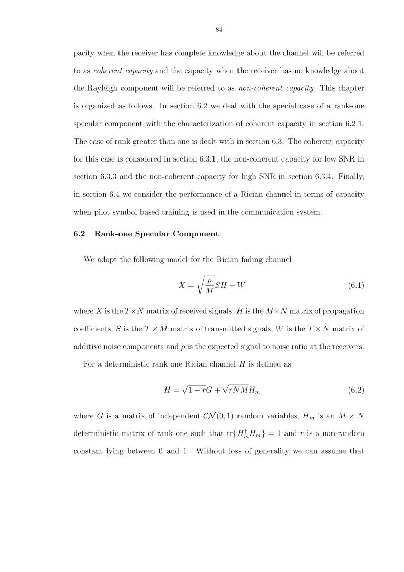
84

pacity when the receiver has complete knowledge about the channel will be referred

to as coherent capacity and the capacity when the receiver has no knowledge about

the Rayleigh component will be referred to as non-coherent capacity. This chapter

is organized as follows. In section 6.2 we deal with the special case of a rank-one

specular component with the characterization of coherent capacity in section 6.2.1.

The case of rank greater than one is dealt with in section 6.3. The coherent capacity

for this case is considered in section 6.3.1, the non-coherent capacity for low SNR in

section 6.3.3 and the non-coherent capacity for high SNR in section 6.3.4. Finally,

in section 6.4 we consider the performance of a Rician channel in terms of capacity

when pilot symbol based training is used in the communication system.

6.2 Rank-one Specular Component

We adopt the following model for the Rician fading channel

X =

√ρ

MSH +W (6.1)

whereX is the T×N matrix of received signals, H is theM×N matrix of propagation

coefficients, S is the T ×M matrix of transmitted signals, W is the T ×N matrix of

additive noise components and ρ is the expected signal to noise ratio at the receivers.

For a deterministic rank one Rician channel H is defined as

H =√1− rG+

√rNMHm (6.2)

where G is a matrix of independent CN (0, 1) random variables, Hm is an M × N

deterministic matrix of rank one such that trH †mHm = 1 and r is a non-random

constant lying between 0 and 1. Without loss of generality we can assume that

85

Hm = αβ† where α is a length M vector and β is a length N vector such that

Hm =

1

0

...

0

[1 0 . . . 0] (6.3)

where the column and row vectors are of appropriate lengths.

In this case, the conditional probability density function of X given S is given by,

p(X|S) = e−tr[IT+(1−r)(ρ/M)SS†]−1(X−√rNMSHm)(X−

√rNMSHm)†

πTN detN [IT + (1− r)(ρ/M)SS†].

The conditional probability density enjoys the following properties

1. For any T × T unitary matrix φ

p(φX|φS) = p(X|S)

2. For any (M − 1)× (M − 1) unitary matrix ψ

p(X|SΨ) = p(X|S)

where

Ψ =

1 0

0† ψ

. (6.4)

6.2.1 Coherent Capacity

The mutual information (MI) expression for the case where H is known by the

receiver has already been derived in [23]. The informed receiver capacity achieving

signal S is zero mean Gaussian independent from time instant to time instant. For

such a signal the MI is

I(X;S|H) = T · E log det[

IN +ρ

MH†ΛH

]

86

where Λ = E[Sτt S

∗t ] for t = 1, . . . , T , St is the tth row of the T ×M matrix S. Sτ

t

denotes the transpose of St and S∗tdef= (Sτ

t )†.

Theorem 6.1. Let the channel H be Rician (6.2) and be known to the receiver.

Then the capacity is

CH = maxl,d

TE log det[IN +ρ

MH†Λ(l,d)H] (6.5)

where the signal covariance matrix Λ(l,d) is of the form

Λ(l,d) =

M − (M − 1)d l1M−1

l1τM−1 dIM−1

where d is a positive real number such that 0 ≤ d ≤ M/(M − 1) and l is such that

|l| ≤√

( MM−1 − d)d. IM−1 is the identity matrix of dimension M −1 and 1M−1 is the

all ones column vector of length M − 1.

Proof: This proof is a modification of the proof in [73]. Using the property that

Ψ†H has the same distribution as H where Ψ is of the form given in (6.4) we conclude

that

T · E log det[

IN +ρ

MH†ΛH

]

= T · E log det[

IN +ρ

MH†ΨΛΨ†H

]

.

If Λ is written as

Λ =

c A

A† B

where c is a positive number such that c ≥ A†B−1A (to ensure positive semi-

definiteness of the covariance matrix Λ), A is a row vector of length M − 1 and

B is a positive definite matrix of size (M − 1)× (M − 1). Then

ΨΛΨ† =

c Aψ†

ψA† ψBψ†

.

87

Since B = UDU † where D is a diagonal matrix and U is a unitary matrix of size

(M − 1)× (M − 1), choosing ψ = ΠU where Π is a (M − 1)× (M − 1) permutation

matrix, we obtain that

T · E log det[

IN +ρ

MH†ΛH

]

= T · E log det[

IN +ρ

MH†ΛΠH

]

where

ΛΠ =

c AU †Π†

ΠUA† ΠDΠ†

.

Since log det is a concave (convex cap) function we have

T · E log det[

IN +ρ

MH† ΛΠ H

]

≥ T · 1

(M − 1)!

∑

Π

E log det[

IN +ρ

MH†ΛΠH

]

= I(X;S)

where ΛΠ = 1(M−1)!

∑

Π ΛΠ and the summation is over all (M − 1)! possible permu-

tation matrices Π. Therefore, the capacity achieving Λ is given by ΛΠ and is of the

form

Λ =

c b1M−1

b1τM−1 dIM−1

where d = trB/(M − 1). Now, the capacity achieving signal matrix has to satisfy

trΛ =M since MI is monotonically increasing in trΛ. Therefore, c =M − (M −

1)d. And since c ≥ L†D−1L this implies M − (M − 1)d ≥ (M−1)|l|2d

and we obtain

the desired signal covariance structure.

The problem remains to find the l and d that achieve the maximum in (6.5).

This problem has an analytical solution for the special cases of: 1) r = 0 for which

d = 1 and l = 0 (rank M signal S); and 2) r = 1 for which d = l = 0 (rank 1

signal S). In general, the optimization problem (6.5) can be solved by using the

method of steepest descent over the space of parameters that satisfy the average

88

power constraint (See Appendix B.1). Results for ρ = 100, 10, 1, 0.1 are shown in

Figure 6.1. The optimum values of l for different values of ρ turned out to be zero,

i.e. the signal energy transmitted is uncorrelated over different antenna elements

and over time. As can be seen from the plot the optimum value of d stays close to 1

for high SNR and close to 0 for low SNR. That is, the optimum covariance matrix is

close to an identity matrix for high SNR. For low SNR, all the energy is concentrated

in the direction of the specular component or in other words the optimal signaling

strategy is beamforming. These observations are proven in section 6.3.1.

0 0.1 0.2 0.3 0.4 0.5 0.6 0.7 0.8 0.9 10

0.2

0.4

0.6

0.8

1

1.2

1.4

r (fraction of energy in the specular component)

d

dB = −20

dB = 0

dB = 20

dB = 40

Figure 6.1: Optimum value of d as a function of r for different values of ρ

6.3 General Rank Specular Component

In this case the channel matrix can be written as

H =√1− rG+

√rHm (6.6)

where G is the Rayleigh Fading component and Hm is a deterministic matrix such

that trHmH†m = MN with no restriction on its rank. Without loss of generality,

we can assume Hm to be an M ×N diagonal matrix with positive real entries.

89

6.3.1 Coherent Capacity

For high SNR, we show that the capacity achieving signal structure basically ig-

nores the specular component. There is no preference given to the channel directions

in the specular component.

Proposition 6.1. Let H be Rician (6.6). Let CH be the capacity for H known at

the receiver. For high SNR ρ, CH is attained by an identity signal covariance matrix

when M ≤ N and

CH = T · E log det[ρ

MHH†] +O(

log(√ρ)

√ρ

).

Proof: The expression for capacity, CH is

CH = T · E log det[IN +ρ

MH†ΛH].

Let H have SVD H = ΦΣΨ† then

log det[IN +ρ

MH†ΛH] = log det[IN +

ρ

MΣ†Φ†ΛΦΣ].

Let Φ†ΛΦ = D. Then

log det[IN +ρ

MΣ†DΣ] = log det[IM +

ρ

MDΣΣ†].

The right hand side expression is maximized by choosing Λ such that D is diagonal

[13, page 255] (We will show finally that the optimum D does not depend on the

specific realization of H). Let D = diagd1, d2, . . . , dM and σi be the eigenvalues

of ΣΣ† and

EA[f(x)]def= E[f(x)χA(x)] (6.7)

90

where χA(x) is the characteristic function for the set A so that χA(x) = 0 if x /∈ A

and χA(x) = 1 otherwise, then for large ρ

E log det[IM +ρ

MDΣΣ†] =

M∑

i=1

Eσi<1/√ρ log[1 +

ρ

Mdiσi] +

M∑

i=1

Eσi≥1/√ρ log[1 +ρ

Mdiσi].

Let K denote the first term in the right hand side of the expression above and L

denote the second term. We can show that

E log det[IM +ρ

MDΣΣ†] = log

ρ

M+

M∑

i=1

log(di) +M∑

i=1

Eσi>1/√ρ[log(σi)] +

O(log(√ρ)/√ρ)

since

K ≤ log[1 +√ρ]

M∑

i=1

P (σi < 1/√ρ) = O(log(

√ρ)/√ρ)

and

L = logρ

M+

M∑

i=1

log(di) +M∑

i=1

Eσi>1/√ρ[log(σi)] +O(1/

√ρ).

On account of log being a convex cap function the first term in the expression on

the last line above is maximized by choosing di = d for i = 1, . . . ,M such that

M · d =M .

For M > N , optimization using the steepest descent algorithm similar to the one

described in Appendix B.1 shows that for high SNR the capacity achieving signal

matrix is an identity matrix as well and the capacity is given by

CH ≈ T · E log det[IN +ρ

MH†H].

For low SNR, we next show that the Rician fading channel essentially behaves like

an AWGN channel in the sense that the Rayleigh fading component has no effect on

the structure of the optimum covariance structure.

91

Proposition 6.2. Let H be Rician (6.6) and let the receiver have complete knowledge

of the Rayleigh component G. For low SNR, CH is attained by the same signal

covariance matrix that attains capacity when r = 1, irrespective of the value of M

and N , and

CH = Tρ[rλmax(HmH†m) + (1− r)N ] +O(ρ2).

Proof: Let ‖H‖ denote the matrix 2-norm of H, γ be a positive number such that

γ ∈ (0, 1) then

CH = T · E log det[IN +ρ

MH†ΛH]

= T · E‖H‖≥1/ργ log det[IN +ρ

MH†ΛH] + E‖H‖<1/ργ log det[IN +

ρ

MH†ΛH]

= TEtr ρMH†ΛH+O(ρ2−2γ)

where E‖H‖≥1/ργ [·] is as defined in (6.7). This follows from the fact that P (‖H‖ ≥

1/ργ) ≤ O(e−1

TMργ ) and for ‖H‖ < 1/ργ log det[IN + ρMH†ΛH] = tr[ ρ

MH†ΛH] +

O(ρ2−2γ). Since γ is arbitrary

E log det[IN +ρ

MH†ΛH] = Etr[

ρ

MH†ΛH] +O(ρ2).

Now

Etr[H†ΛH] = tr(1− r)E[G†ΛG] + rH†mΛHm]

= tr(1− r)ΛE[GG†] + rΛHmH†m.

Therefore, we have to choose Λ to maximize tr(1− r)NΛ + rΛHmH†m. Since Hm

is diagonal the trace depends only on the diagonal elements of Λ. Therefore, Λ

can be chosen to be diagonal. Also, because of the power constraint, trΛ ≤M , to

maximize the expression we choose trΛ =M . The maximizing Λ has as many non-

zero elements as the multiplicity of the maximum eigenvalue of (1−r)NIM+rHmH†m.

92

The non-zero elements of Λ multiply the maximum eigenvalues of (1 − r)NIM +

rHmH†m and can be chosen to be of equal magnitude summing up to M . This is

the same Λ maximizing the capacity for additive white Gaussian noise channel with

channel Hm.

Note that if we choose Λ = IM then varying r has no effect on the value of the

capacity. This explains the trend seen in Figures 4.2 and 4.3 in Chapter 4 and Figures

5.1 and 5.2 in Chapter 5.

6.3.2 Non-Coherent Capacity Upper and Lower Bounds

It follows from the data processing theorem that the non-coherent capacity, C can

never be greater than the coherent capacity CH , that is, the uninformed capacity is

never decreased when the channel is known to the receiver.

Proposition 6.3. Let H be Rician (6.6) and the receiver have no knowledge of the

Rayleigh component then

C ≤ CH .

Now, we establish a lower bound which is similar in flavor to those derived in

chapters 4 and 5.

Proposition 6.4. Let H be Rician (6.6). A lower bound on capacity when the

receiver has no knowledge of G is

C ≥ CH −NE[

log2 det(

IT + (1− r) ρMSS†

)]

(6.8)

≥ CH −NM log2(1 + (1− r) ρMT ). (6.9)

Proof: Proof is similar to that of Proposition 5.2 in Chapter 5 and won’t be

repeated here.

93

We notice that the second term in the lower bound goes to zero when r = 1:

as the channel becomes purely Gaussian the capacity of the channel is completely

determined.

6.3.3 Non-Coherent Capacity: Expressions for Low SNR

In this section, we introduce some new notation for ease of description. if X is a

T ×N matrix then let X denote the “unwrapped” NT × 1 vector formed by placing

the transposed rows of X in a single column in an increasing manner. That is, if Xi,j

denotes the element of X in the ith row and jth column then Xi,1 = Xbi/Nc,i%N . The

channel model X =√

ρMSH +W can now be written as X =

√ρMHS + W . H is

given by H = IT ⊗Hτ where Hτ denotes the transpose of H. The notation A ⊗ B

denotes the Kronecker product of the matrices A and B and is defined as follows. If

A is a I × J matrix and B a K × L matrix then A⊗B is a IK × JL matrix

A⊗B =

(A)11B (A)12B . . . (A)1JB

(A)21B (A)22B . . . (A)2JB

......

. . ....

(A)I1B (A)I2B . . . (A)IJB

.

This way, we can describe the conditional probability density function p(X|S) as

follows

p(X|S) = 1

πTN |ΛX|S|e−(X−

√r ρM

HmS)†Λ−1

X|S(X−√

r ρM

HmS)

where |ΛX|S| = det(ITN + (1− r)SS† ⊗ IN).

For low SNR, it will be shown that the channel behaves as an AWGN channel.

Calculation of capacity for the special case of peak power constraint has been shown

in Appendix B.2.

Theorem 6.2. Let the channel H be Rician (6.6) and the receiver have no knowledge

94

of G. For fixed M , N and T if S is a Gaussian distributed source then as ρ→ 0

I(X;SG) = rTρλmax(HmH†m) +O(ρ2)

where I(X;SG) is the mutual information between the output and the Gaussian

source.

Proof: First, I(X;S) = H(X) − H(X|S). Since S is Gaussian distributed,

E[log det(IN + ρMHΛSH

†)] ≤ H(X) ≤ log det(IN + ρMΛX) where the expectation

is taken over the distribution of H and HΛSH† = ΛX|H is the covariance of X

for a particular H. Next, we show that H(X) = ρMtrΛX + O(ρ2). First, the

upper bound to H(X) can be written as ρMtrΛX + O(ρ2) because H is Gaus-

sian distributed and the probability that ‖H‖ > R is of the order e−R2. Second,

E[log det(ITN + ρMHΛSH

†)] = E‖H‖<(Mρ)γ [·]+E‖H‖≥(M

ρ)γ [·] where γ is a number such

that 2− γ > 1 or γ < 1. Then

E[log det(ITN +ρ

MHΛSH

†)] =ρ

ME‖H‖<(M

ρ)γ [trHΛSH

†] +

O(ρ2−γ) +O(log((M

ρ)γ)e−(

Mρ)γ )

=ρ

ME[trHΛH†] +O(ρ2−γ).

Since γ is arbitrary, we have H(X) = ρME[trHΛSH

†] + O(ρ2). Note that ΛX =

E[ΛX|H ] and sinceH(X) is sandwiched between two expressions of the form ρMtrΛX+

O(ρ2) the assertion follows.

Calculate H(X|S) = E[log det(ITN + (1 − r) ρMSS† ⊗ IN)]. We have S to be

Gaussian distributed therefore in a similar manner it can be shown that H(X|S) =

(1− r) ρMtrE[SS† ⊗ IN ]+O(ρ2).

H =√rHm+

√1− rG therefore, ΛX = E[HΛSH

†] = rHmΛSH†m+(1−r)E[SS†]⊗

IN . Therefore, we have for a Gaussian distributed input I(X;SG) = r ρMtrHmΛSH

†m+

95

O(ρ2). Since Hm is a diagonal matrix only the diagonal elements of ΛS matter.

Therefore, we can choose the signals to be independent from time instant to time

instant. Also, to maximize trHmΛSH†m under the condition trΛ ≤ TM it is best

to concentrate all the available energy on the largest eigenvalues of Hm. Therefore,

we obtain

I(X;SG) = rρ

MTMλmax(HmH

†m) +O(ρ2).

Corollary 6.1. For purely Rayleigh fading channels when the receiver has no knowl-

edge of G a Gaussian transmitted signal satisfies limρ→0 I(X;SG)/ρ = 0.

The peak constraint results in Appendix B.2 and the Gaussian input results imply

that for low SNR Rayleigh fading channels are at a disadvantage compared to Rician

fading channels. But, it has been shown in [2, 75] for single antenna transmit and

receive channel Rayleigh fading provides as much capacity as a Gaussian channel

with the same energy for low SNR. We will extend that result to multiple transmit

and receive antenna channel for the general case of Rician fading. The result for

Rayleigh fading will follow as a special case.

Theorem 6.3. Let H be Rician (6.6) and the receiver have no knowledge of G. For

fixed M , N and T

limρ→0

C

ρ= T

[rλmax(HmH

†m) +N(1− r)

].

Proof: First, absorb√

ρM

into S and rewrite the channel as

X = HS +W

with the average power constraint on the signal S E[trSS†] ≤ ρMTM = ρT .

96

It has been shown [75] that if the input alphabet includes the value “0” (symbol

with 0 power) for a channel with output X, and condition probability given by

p(X|S), then

limPC→0

C

PC

= sups∈S

D( p(X|S = s) ‖ p(X|S = 0) )

Ps

where S is the set of values that the input can take, PC is the average power constraint

on the input (in our case, E[trSS†] ≤ PC = ρT ) and Ps = trss† is the energy

in the specific realization of the input S = s and D(pA‖pB) is the Kullback-Leibler

distance for continuous density functions with argument x defined as

D(pA‖pB) =∫

pA(x) logpA(x)

pB(x)dx.

Applying the above result to the case of Rician fading channels, we obtain

limρ→0

C

ρT= sup

S

D( p(X|S) ‖ p(X|0) )trSS†

.

First, we have

p(X|S) = 1

πTN |ΛX|S|e−(X−√rHmS)† Λ−1

X|S(X−√rHmS)

and

p(X|0) = 1

πTNe−X†X .

Therefore,

D( p(X|S) ‖ p(X|0) ) =

∫

p(X|S)[

log1

|ΛX|S|+ X†X −

(

X −√rHmS)†

Λ−1X|S

(

X −√rHmS)]

dX

= log1

|ΛX|S|+ tr

rHmSS†H†

m + ΛX|S

− TN

= log1

det(ITN + (1− r)SS† ⊗ IN)+

tr

rHmSS†H†

m + (1− r)SS† ⊗ IN

.

97

This gives,

D( p(X|S) ‖ p(X|0) )trSS†

= −N∑T

i=1 log(1 + λi(SS†))

∑Ti=1 λi(SS†)

+trrHmSS

†H†m

∑Ti=1 trSiS

†i

+

N(1− r)

where we have used the facts that det(ITN+(1−r)SS†⊗IN) = det(IT +(1−r)SS†)N ,

trSS† = trSS† =∑Ti=1 trSτ

i S∗i where Si is the i

th row in the matrix S.

Since,

HmSS†H†

m =

HτmS

τ1S

∗1H

∗m Hτ

mSτ1S

∗2H

∗m . . . Hτ

mSτ1S

∗TH

∗m

HτmS

τ2S

∗1H

∗m Hτ

mSτ2S

∗2H

∗m . . . Hτ

mSτ2S

∗TH

∗m

......

. . ....

HτmS

τTS

∗1H

∗m Hτ

mSτTS

∗2H

∗m . . . Hτ

mSτTS

∗TH

∗m

we have trHmSS†H†

m =∑T

i=1 trHτmS

τi S

∗iH

∗m = trH∗

mHτm

∑Ti=1 S

τi S

∗i . There-

fore,

D( p(X|S) ‖ p(X|0) )trSS†

= −N∑N

i=1 log(1 + λi(S†S))

∑Ni=1 λi(S†S)

+ rtrH∗

mHτm

∑Ti=1 S

τi S

∗i

∑Ti=1 trSτ

i S∗i

+

N(1− r).

Note that since Hm is a diagonal matrix only the diagonal elements of SiS†i affect the

second term. Therefore, for a given∑T

i=1 Sτi S

∗i the second term in right hand side of

the expression above can be maximized by choosing Si such that Sτi S

∗i is diagonal. In

addition the non-zero values of SiS†i should be located at the same diagonal positions

as the maximum entries of H∗mH

τm. In such a case the expression above evaluates to

D( p(X|S) ‖ p(X|0) )trSS†

= −N log(1 + trS†S)trS†S + rλmax(H

∗mH

τm) +N(1− r).

The first term can be made arbitrarily small by letting trS†S → ∞. Therefore,

we have limρ→0CρT

= rλmax(HmH†m) +N(1− r).

98

Theorem 6.3 suggests that at low SNR all the energy has to be concentrated in the

strongest directions of the specular component. In [2] it is shown that the optimum

signaling scheme for Rayleigh fading channels is an “on-off” signaling scheme. We

conjecture that the capacity achieving signaling scheme for low SNR in the case of

the Rician fading is also a similar “on-off” signaling scheme.

6.3.4 Non-Coherent Capacity: Expressions for High SNR

In this section we apply the method developed in [85] for the analysis of Rayleigh

fading channels. The only difference in the models considered in [85] and here is that

we assume H has a deterministic non-zero mean. For convenience, we use a different

notation for the channel model. We rewrite the channel model as

X = SH +W

with H =√rHm +

√1− rG where Hm is the specular component of H and G

denotes the Rayleigh component. G andW consist of Gaussian circular independent

random variables and the covariance matrices of G and W are given by (1− r)IMN

and σ2ITN , respectively. Hm is deterministic such that E[trHH†] =MN and r is

a number between 0 and 1.

Lemma 6.1. Let the channel be Rician (6.6) and the receiver have no knowledge of

G. Then the capacity achieving signal, S can be written as S = ΦVΨ† where Φ is a

T ×M unitary matrix independent of V and Ψ. V and Ψ are M ×M .

Proof: Follows from the fact that p(ΦX|ΦS) = p(X|S).

In [85] the requirement for X = SH +W was that X had to satisfy the property

that in the singular value decomposition of X, X = ΦVΨ† Φ be independent of V

and Ψ. This property holds for the case of Rician fading too because the density

functions of X, SH and S are invariant to pre-multiplication by a unitary matrix.

99

Therefore, the leading unitary matrix in the SVD decomposition of any of X, SH

and S is independent of the other two components in the SVD and isotropically

distributed.

Therefore, Lemma 6 in [85] holds

Lemma 6.2. Let R = ΦRΣRΨ†R be such that ΦR is independent of ΣR and ΨR. Then

H(R) = H(QΣRΨ†R) + log |G(T,M)|+ (T −M)E[log detΣ2

R]

where Q is an M ×M unitary matrix independent of V and Ψ and |G(T,M)| is the

volume of the Grassmann Manifold and is equal to

∏Ti=T−M+1

2πi

(i−1)!∏M

i=12πi

(i−1)!.

The Grassmann Manifold G(T,M) [85] is the set of equivalence classes of all T×M

unitary matrices such that if P,Q belong to an equivalence class then P = QU for

some M ×M unitary matrix U .

M = N , T ≥ 2M

To calculate I(X;S) we need to computeH(X) andH(X|S). To computeH(X|S)

we note that given S, X is a Gaussian random vector with columns of X independent

of each other. Each row has the common covariance matrix given by (1 − r)SS† +

σ2IT = ΦV 2Φ† + σ2IT . Therefore

H(X|S) =ME[M∑

i=1

log(πe((1− r)‖si‖2 + σ2)] +M(T −M) log(πeσ2).

To compute H(X), we write the SVD: X = ΦXΣXΨ†X . Note that ΦX is isotropi-

cally distributed and independent of ΣXΨ†X , therefore from Lemma 6.2 we have

H(X) = H(QΣXΨ†X) + log |G(T,M)|+ (T −M)E[log detΣ2

X ].

We first characterize the optimal input distribution in the following lemma.

100

Lemma 6.3. Let H be Rician (6.6) and the receiver have no knowledge of G. Let

(sσi , i = 1, . . . ,M) be the optimal input signal of each antenna at when the noise

power at the receive antennas is given by σ2. If T ≥ 2M ,

σ

‖sσi ‖P−→ 0, for i = 1, . . . ,M (6.10)

whereP−→ denotes convergence in probability.

Proof: See Appendix B.3.

Lemma 6.4. Let H be Rician (6.6) and the receiver have no knowledge of G.

The maximal rate of increase of capacity, maxp(S):E[trSS†]≤TM I(X;S) with SNR

is M(T −M) log ρ and the constant norm source ‖si‖2 = T for i = 1, . . . ,M attains

this rate.

Proof: See Appendix B.3.

Lemma 6.5. Let H be Rician (6.6) and the receiver have no knowledge of G. As

T →∞ the optimal source in Lemma 6.4 is the constant norm input

Proof: See Appendix B.3.

From now on, we assume that the optimal input signal is the constant norm input.

For the constant norm input ΦVΨ† = ΦV since Φ is isotropically distributed.

Theorem 6.4. Let the channel be Rician (6.6) and the receiver have no knowledge

of G. For the constant norm input, as σ2 → 0 the capacity is given by

C = log |G(T,M)|+ (T −M)E[log detH †H]−M(T −M) log πeσ2 −

M2 log πe+H(QVH) + (T − 2M)M log T −M 2 log(1− r)

where Q, V and |G(T,M)| are as defined in Lemma 6.2.

101

Proof: Since ‖s2i ‖ À σ2 for all i = 1, . . . ,M

H(X|S) = ME[M∑

i=1

log πe((1− r)‖si‖2 + σ2)] +M(T −M) log(πeσ2)

≈ ME[M∑

i=1

log πe(1− r)‖si‖2] +M(T −M) log πeσ2

= ME[log det(1− r)V 2] +M 2 log πe+M(T −M) log πeσ2

and from Appendix B.5

H(X) ≈ H(SH)

= H(QVH) + log |G(T,M)|+ (T −M)E[log det(H †V 2H)]

= H(QVH) + log |G(T,M)|+ (T −M)E[log detV 2] +

(T −M)E[log detHH†].

Combining the two equations

I(X;S) ≈ log |G(T,M)|+ (T −M)E[log detH †H]−M(T −M) log πeσ2 +

H(QVH)−M 2 log πe+ (T − 2M)E[log detV 2]−M 2 log(1− r).

Now, since the optimal input signal is ‖si‖2 = T for i = 1, . . . ,M , we have

C = I(X;S)

≈ log |G(T,M)|+ (T −M)E[log detH†H]−M(T −M) log πeσ2 −

M2 log πe+H(QVH) + (T − 2M)M log T −M 2 log(1− r).

Theorem 6.5. Let H be Rician (6.6) and the receiver have no knowledge of G. As

T →∞ the normalized capacity C/T → E[log det ρMH†H] where ρ =M/σ2.

102

Proof: First, a lower bound to capacity as σ2 → 0 is given by

C ≥ log |G(T,M)|+ (T −M)E[log detH †H] +M(T −M) logTρ

Mπe−

M2 log T −M 2 log(1− r)−M 2 log πe.

In [85] it’s already been shown that limT→∞( 1Tlog |G(T,M)|+M(1− M

T) log T

πe) =

0. Therefore we have as T →∞

C/T ≥ME[log detρ

MH†H].

Second, since H(QVH) ≤ M 2 log(πeT ) an asymptotic upper bound on capacity

is given by

C ≤ log |G(T,M)|+ (T −M)E[log detH †H] +M(T −M) logTρ

Mπe−

M2 log(1− r).

Therefore, we have as T →∞

C/T ≤ E[log detρ

MH†H].

M < N T ≥M +N

In this case we show that the optimal rate of increase is given by M(T −M) log ρ.

The higher number of receive antennas can provide only a finite increase in capacity

for all SNRs.

Theorem 6.6. Let the channel be Rician (6.6) and the receiver have no knowledge

of G. Then the maximum rate of increase of capacity with respect to log ρ is given

by M(T −M).

Proof: See Appendix B.3.

103

6.4 Training in Non-Coherent Communications

It is important to know whether training based signal schemes are practical and if

they are how much time can be spent in learning the channel and what the optimal

training signal is like. Hassibi and Hochwald [39] have addressed these issues for the

case of Rayleigh fading channels. They showed that 1) pilot symbol training based

communication schemes are highly suboptimal for low SNR and 2) when practical the

optimal amount of time devoted to training is equal to the number of transmitters,

M when the fraction of power devoted to training is allowed to vary and 3) the

orthonormal signal is the optimal signal for training.

In [85] the authors demonstrate a very simple training method that achieves the

optimal rate of increase with SNR. The same training method can also be easily

applied to the Rician fading model with deterministic specular component. The

training signal is the M ×M diagonal matrix dIM . d is chosen such that the same

power is used in the training and the communication phase. Therefore, d =√M .

Using S = dIM , the output of the MIMO channel in the training phase is given by

X =√M√rHm +

√M√1− rG+W

The Rayleigh channel coefficients G can be estimated independently using scalar

minimum mean squared error (MMSE) estimates since the elements of W and G are

i.i.d. Gaussian random variables

G =

√1− r

√M

(1− r)M + σ2[X −

√M√rHm]

where recall that σ2 is the variance of the components of W . The elements of the

estimate G are i.i.d. Gaussian with variance (1−r)M(1−r)M+σ2 . Similarly, the estimation

error matrix G − G has i.i.d Gaussian distributed elements with zero mean and

variance σ2

(1−r)M+σ2 .

104

The output of the channel in the communication phase is given by

X = SH +W

=√rSHm +

√1− rSG+

√1− rS(G− G) +W

where S consists of zero mean i.i.d circular Gaussian random variables with zero

mean and unit variance. This choice of S is sub-optimal as this might not be the

capacity achieving signal, but this choice gives us a lower bound on capacity. Let

W =√1− rS(G − G) +W . For the choice of S given above the entries of W are

uncorrelated with each other and also with S(√rHm +

√1− rG). The variance of

each of the entries of W is given by σ2 + (1− r)M σ2

(1−r)M+σ2 . If W is replaced with

a white Gaussian noise with the same covariance matrix then the resulting mutual

information is a lower bound on the actual mutual information [13, p. 263]. This

result is formally stated in Proposition 6.5. In this section we deal with normalized

capacity C/T instead of capacity C. The lower bound on the normalized capacity is

given by

C/T ≥ T − Tt

TE log det

(

IM +ρeffM

H1H†1

)

where ρeff in the expression above is the effective SNR at the output (explained at

the end of this paragraph), and H1 is a Rician channel with a new Rician parameter

rnew where rnew = r

r+(1−r)(1−r)M

(1−r)M+σ2

. This lower bound can be easily calculated because

the lower bound is essentially the coherent capacity with H replaced by√rnewHm +

√1− rnewG. The signal covariance structure was chosen to be an identity matrix

as this is the optimum covariance matrix for high SNR. The effective SNR is now

given by the ratio of the energy of the elements of S(√rHm +

√1− rG) to the

energy of the elements of W . The energy in the elements of S(√rHm +

√1− rG)

is given by M(r + (1− r)2 M(1−r)M+σ2 ) and the energy in the elements of W are given

105

by σ2 + (1−r)Mσ2

(1−r)M+σ2 . Therefore, the effective SNR, ρeff is given by ρ[r+r(1−r)ρ+(1−r)2ρ][1+2(1−r)ρ]

where ρ = Mσ2 is the actual SNR. Note, for r = 1 no training is required since the

channel is completely known.

This simple scheme achieves the optimum increase of capacity with SNR and uses

only M of the T symbols for training.

We will compare the LMS algorithm for estimation of the channel coefficients to

this simple scheme. LMS is obviously at a disadvantage because when σ2 = 0 the

simple scheme outlined above generates a perfect channel estimate after M training

symbols whereas the LMS algorithm requires much more than M training symbols

to obtain an accurate estimate. The performance of the simple training scheme is

plotted with respect to different SNR values for comparison with the asymptotic

upper bound to capacity in the proof of Theorem 6.5. The plot also verifies the

result of Theorem 6.5. The plots are for M = N = 5, r = 0.9 and T = 50 in Figure

6.2 the specular component is a rank-one specular component given by (6.3).

0 50 100 150 200 250 300 350 400−50

0

50

100

150

200

250

300

350

SNR (dB)

Cap

acity

(bits

/T)

Coherent Capacity

Training Lower Bound

Capacity

Figure 6.2: Asymptotic capacity upper bound, Capacity Upper and Lower bounds for differentvalues of SNR

106

We can quantify the amount of training required using the techniques in [39]. In

[39], the authors use the optimization of the lower bound on capacity to find the

optimal allocation of training as compared to communication. Let Tt denote the

amount of time devoted to training and Tc the amount of time devoted to actual

communication. Let St be the Tt ×M signal used for training and Sc the Tc ×M

signal used for communication.

Let κ denote the fraction of the energy used for communication. Then T = Tt+Tc

and trStS†t = (1− κ)TM and trScS

†c = κTM .

Xt = St(√rHm +

√1− rG) +Wt

Xc = Sc(√rHm +

√1− rG) +Wc

where Xt is Tt ×N and Xc is Tc ×N . G is estimated from the training phase. For

that we need Tt ≥ M . Since G and Wt are Gaussian the MMSE estimate of G is

also the linear MMSE estimate conditioned on S. The optimal estimate is given by

G =√1− r(σ2IM + (1− r)S†tSt)

−1S†t (Xt −√rStHm).

Let G = G− G then

Xc = Sc(√rHm +

√1− rG) +

√1− rScG+Wc.

Let Wc =√1− rStG +W . Note that elements of Wc are uncorrelated with each

other and have the same marginal densities when the elements of Sc are chosen to be

i.i.d Gaussian. If we replace Wc with Gaussian noise that is zero-mean and spatially

and temporally independent the elements of which have the same variance as the

elements of Wc then the resulting mutual information is a lower bound to the actual

mutual information in the above channel. This is stated formally in the following

proposition.

107

Proposition 6.5 (Theorem 1 in [39]). Let

X = SH +W

be a Rician fading channel with H known to the receiver. Let S and W satisfy

1ME[SS†] = 1 and 1

ME[WW †] = σ2 and be uncorrelated with each other. Then the

worst case noise has i.i.d. zero mean Gaussian distribution, i.e. W ∼ CN (0, IN ).

Moreover, this distribution has the following minimax property

IW∼CN (0,σ2IN ),S(X;S) ≤ IW∼CN (0,σ2IN ),S∼CN (0,IM )(X;S) ≤ IW,S∼CN (0,IM )(X;S)

where IW∼CN (0,σ2IN ),S(X;S) denotes the mutual information between X and S when

W has a zero mean complex circular Gaussian distribution and S has any arbitrary

distribution.

The variance of the elements of Wc is given by

σ2wc = σ2 +1− rNTc

trE[GG†]κTIM

= σ2 +(1− r)κTM

Tc

1

NMtrE[GG†]

= σ2 +(1− r)κTM

Tc

σ2G

and the lower bound is

Ct/T ≥T − Tt

TE log det

(

IM +ρeffM

H1ΛH†1

)

(6.11)

where ρeff is the ratio of the energies in the elements of ScH and energies in the

elements of Wc and H1 =√rnewHm +

√1− rnewG where rnew = r

r+(1−r)σ2G

. Λ is the

optimum signal correlation matrix the form of which depends on the distribution of

H1 according to Proposition 6.2 for low SNR and Proposition 6.1 for high SNR and

M ≤ N as given in section 6.3.1.

108

To calculate ρeff , the energy in the elements of SH is given by

σ2SH =1

NTc

[rtrHmH†mκTIM+ (1− r)trGG†κTIM]

=κTM

Tc

1

NM[rNM + (1− r)trGG†]

=κTM

Tc

[r + (1− r)σ2G]

which gives us

ρeff =κTρ[r + (1− r)σ2

G]

Tc + (1− r)κTρσ2G

.

6.4.1 Optimization of St, κ and Tt

We will optimize St, κ and Tt to maximize the lower bound (6.11). In this section

we merely state the main results and their interpretations. Derivations and details

are given in the Appendices.

Optimization of the lower bound over St is difficult as St effects the distribution

of H, the form of Λ as well as ρeff . To make the problem simpler we will just find

the value of St that maximizes ρeff .

Theorem 6.7. The signal St that maximizes ρeff satisfies the following condition

S†tSt = (1− κ)TIM

and the corresponding ρeff is

ρ∗eff =κTρ[Mr + ρ(1− κ)T ]

Tc(M + ρ(1− κ)T ) + (1− r)κTρM .

Proof: See Appendix B.6.

The optimum signal derived above is the same as the optimum signal derived in

[39].

109

The corresponding capacity lower bound using the St obtained above is

Ct/T ≥T − Tt

TE log det

(

IM +ρeffM

H1ΛH†1

)

where ρeff is as given above and H1 =√rnewHm +

√1− rnewG where rnew =

r1+(1−r)(1−κ) ρ

MT

r+(1−r)(1−κ) ρM

Tand as before G is a matrix consisting of i.i.d. Gaussian circular

random variables with mean zero and unit variance. Now, Λ is the covariance ma-

trix of the source Sc when the channel is Rician and known to the receiver. The form

of Λ was derived for ρeff → 0 and ρeff →∞ in section 6.3.1.

Optimization of (6.11) over κ is straightforward as κ affects the lower bound only

through ρeff and can be stated in the following proposition.

Theorem 6.8. For fixed Tt and Tc the optimal power allocation κ in a training based

scheme is given by

κ =

minγ −√

γ(γ − 1− η), 1 for Tc > (1− r)M

min12+ rM

2Tρ, 1 for Tc = (1− r)M

minγ +√

γ(γ − 1− η), 1 for Tc < (1− r)M

where γ = MTc+TρTcTρ[Tc−(1−r)M ]

and η = rMTρ. The corresponding lower bound is given by

Ct/T ≥T − Tt

TE log det

(

IM +ρeffM

H1ΛH†1

)

where for Tc > (1− r)M

ρeff =

TρTc−(1−r)M

(√γ −√γ − 1− η)2 when κ = γ −

√

γ(γ − 1− η)rρ

1+(1−r)ρwhen κ = 1

for Tc = (1− r)M

ρeff =

T 2ρ2

4(1−r)M(M+Tρ)(1 + rM

Tρ)2 when κ = 1

2+ rM

2Tρ

rTρ(1−r)(M+Tρ)

when κ = 1

110

and for Tc < (1− r)M

ρeff =

Tρ(1−r)M−Tc

(√−γ −√−γ + 1 + η)2 when κ = γ +

√

γ(γ − 1− η)rρ

1+(1−r)ρwhen κ = 1

and rnew is given by substituting the appropriate value of κ in the expression

r1 + (1− r)(1− κ) ρ

MT

r + (1− r)(1− κ) ρMT.

Proof: See Appendix B.7.

For optimization over Tt we draw somewhat similar conclusions as in [39]. In [39]

the optimal setting for Tt was shown to be Tt =M for all values of SNR. We however

show that for small SNR the optimal setting is Tt = 0 or that no training is required.

When training is required, the intuition is that increasing Tt linearly decreases the

capacity through the term (T−Tt)/T , but only logarithmically increases the capacity

through the higher effective SNR ρeff [39]. Therefore, it makes sense to make Tt as

small as possible. For small SNR we show that κ = 1. It is clear that optimization of

Tt makes sense only when κ is strictly less than 1. When κ = 1 no power is devoted

to training and Tt can be made as small as possible which is zero. When κ < 1 the

smallest value Tt can be isM since it takes atleast that many intervals to completely

determine the unknowns.

Theorem 6.9. The optimal length of the training interval is Tt =M whenever κ < 1

for all values of ρ and T > M , and the capacity lower bound is

Ct/T ≥T −MT

E log det(

IM +ρeffM

H1ΛH†1

)

(6.12)

where

ρeff =

TρT−(2−r)M

(√γ −√γ − 1− η)2 for T > (2− r)M

T 2ρ2

4(1−r)M(M+Tρ)(1 + rM

Tρ)2 for T = (2− r)M

TρT−(2−r)M

(√−γ −√−γ + 1 + η)2 for T < (2− r)M

111

The optimal power allocations are easily obtained from Theorem 6.8 by simply setting

Tc = T −M .

Proof: See Appendix B.8

6.4.2 Equal training and data power

As stated in [39], sometimes it is difficult for the transmitter to assign different

powers for training and communication phases. In this section, we will concentrate on

setting the training and communication powers equal to each other in the following

sense

(1− κ)TTt

=κT

Tc

=κT

T − Tt

= 1

this means κ = 1− Tt/T and that the power transmitted in Tt and Tc are equal.

In this case,

ρeff =ρ[r + ρ Tt

M]

1 + ρ[ TtM

+ (1− r)]and the capacity lower bound is

Ct/T ≥T − Tt

TE log det(IM +

ρeffM

H1ΛH†1)

where ρeff is as given above and H1 =√rnewHm +

√1− rnewG where rnew =

r1+(1−r) ρ

MTt

r+(1−r) ρM

Tt.

6.4.3 Numerical Comparisons

Throughout the section we have chosen the number of transmit antennas M, and

receive antennas N, to be equal and Hm = IM .

The Figures 6.3 and 6.4 show rnew and κ respectively as a function of r for different

values of SNR. The plots have been calculated for a block length given by T = 40 and

the number of transmit and receive antennas given byM = N = 5. Figure 6.3 shows

that for low SNR values the channel behaves like a purely AWGN channel given by

112

√rHm and for high SNR values the channel behaves exactly like the original Rician

fading channel. Figure 6.4 shows that as the SNR goes to zero less and less power is

allocated for training. This agrees with the plot in Figure 6.3.

0 0.1 0.2 0.3 0.4 0.5 0.6 0.7 0.8 0.9 10

0.2

0.4

0.6

0.8

1

r

dB = 20

dB = 0

dB = −20

r new

Figure 6.3: Plot of rnew as a function of Rician parameter r

0 0.1 0.2 0.3 0.4 0.5 0.6 0.7 0.8 0.9 10.5

0.6

0.7

0.8

0.9

1

1.1

r

kapp

a

dB = 20

dB = 0

dB = −20

Figure 6.4: Plot of optimal energy allocation κ as a function of Rician parameter r

In Figure 6.5 we plot the training and communication powers for M = N = 10

and dB = 18 for different values of r. We see that as r goes to 1 less and less

113

0 20 40 60 80 100 120 140 160 180 20014

15

16

17

18

19

20

21

22

23

24

Block length T

SN

R (d

B)

r = 0

r = 0.5 r = 0.9

Training

Communication

Figure 6.5: Plot of optimal power allocation as a function of T

power is allocated to the training phase. This makes sense as the proportion of the

energy through the specular component increases there is less need for the system to

estimate the unknown Rayleigh component.

0 5 10 15 20 25 30 35 400

5

10

15

20

25

30

35

40

Block length T

Cap

acity

(bits

/T)

r = 0 r = 0.5

r = 0.7

Capacity lower bounds

Capacity upper bounds

Figure 6.6: Plot of capacity as a function of number of transmit antennas for a fixed T

Figure 6.6 shows capacity as a function of the number of transmit antennas for a

fixed block length T = 40 when dB = 0 and N = 40. We can easily see calculate the

114

optimum number of transmit antennas from the figure. In this case, we see that for

a fixed T the optimum number of transmit antennas increases as as r increases. This

shows that as r goes to 1 there is a lesser need to estimate the unknown Rayleigh

part of the channel and this agrees very well with Figure 6.5 and Figure 6.7 as well

which shows that the optimal amount of training decreases as r increases. Figure

6.7 shows the optimal training period as a function of the block length for the case

of equal transmit and training powers.

20 30 40 50 60 70 800

5

10

15

20

25

Block length T

Opt

imal

trai

ning

per

iod

T t

r = 0.7

r = 0

r = 0.5

dB = 0M = N = 10

Figure 6.7: Optimal Tt as a function of T for equal transmit and training powers

6.4.4 Effect of Low SNR on Capacity Lower Bound

Let’s consider the effect of low SNR on the optimization of κ when r 6= 0. For

Tc > (1− r)M , as ρ→ 0 it is easy to see that γ −√

γ(γ − 1− η)→∞. Therefore,

we conclude that for small ρ we have κ = 1. Similarly, for Tc = (1 − r)M and

Tc < (1− r)M . Therefore, the lower bound tells us that no energy need be spent on

training for small ρ. Also, the form of Λ is known from section 6.3.1.

Evaluating the case where the training and transmission powers are equal we come

to a similar conclusion. For small ρ, ρeff ≈ rρ which is independent of Tt. Therefore,

115

the best value of Tt is Tt = 0. Which also means that we spend absolutely no time

on training. This is in stark contrast to the case when r = 0. In this case, for low

SNR Tt = T/2 [39] and ρeff behaves as O(ρ2).

Note that in both cases of equal and unequal power distribution between training

and communication phases the signal distribution during data transmission phase is

Gaussian. Therefore, the lower bound behaves as rρλmaxHmH†m. Also, rnew = 1

for small ρ showing that the channel behaves as a purely Gaussian channel.

All the conclusions above mimic those of the capacity results with Gaussian input

in section 6.3.3. The low SNR non-coherent capacity results for the case of a Gaussian

input tell us that the capacity behaves as rρλmax with Gaussian input. Moreover,

the results in [39] also agree with the results derived in section 6.3.3. We showed that

for purely Rayleigh fading channels with Gaussian input the capacity behaves as ρ2

which is what the lower bound results in [39] also show. This makes sense because

the capacity lower bound assumes that the signaling input during communication

period is Gaussian. This shows that the lower bound derived in [39] and extended

here is quite tight for low SNR values.

6.4.5 Effect of High SNR on Capacity Lower Bound

For high SNR, γ becomes TcTc−(1−r)M

and the optimal power allocation κ becomes

κ =

√Tc√

Tc +√

(1− r)M

and

ρeff =T

(√Tc +

√

(1− r)M)2ρ.

In the case of equal training and transmit powers, we have for high ρ

ρeff = ρTt

Tt +M(1− r) .

116

For high SNR, the channel behaves as if it is completely known to the receiver.

Note that in this case rnew = r and Λ is an identity matrix for the case M ≤ N .

From the expressions for ρeff given above we conclude that unlike the case of low

SNR the value of r affects the amount of time and power devoted for training.

Let’s look at the capacity lower bound for high SNR. The optimizing Λ in this

regime is an identity matrix. We know that at high SNR the optimal training period

is M . Therefore, the resulting lower bound is given by

Ct/T ≥T −MT

E log det

IM +

ρ(√

1− MT+√

(1−r)MT

)2

HH†

M

.

Note that the lower bound has H figuring in it instead of H1. That is so because for

high SNR, rnew = r. This lower bound can be optimized over the number of transmit

antennas used in which case the lower bound can be rewritten as

Ct/T ≥ maxM ′≤M

max

n≤

M

M ′

T −M ′

TE log det

IM ′ +

ρ(√

1− M ′

T+√

(1−r)M ′

T

)2

HnHn†

M ′

where now Hn is the nth matrix out of a possible M choose M ′ (the number of

ways to choose M ′ transmit elements out of a maximum M elements) matrices of

size M ′ × N . Let Q = minM ′, N and λni be an arbitrary nonzero eigenvalue of

1(√

1−M′

T+

√(1−r)M ′

T

)2HnHn†

M ′ then we have

Ct/T ≥ maxM ′≤M

max

n≤

M

M ′

(

1− M ′

T

) Q∑

i=1

E log(1 + ρλni ).

117

At high SNR, the leading term involving ρ in∑Q

i=1E log(1 + ρλi) is Q log ρ which is

independent of n. Therefore,

Ct/T ≥ maxM ′≤M

(1− M ′

T)M ′ log ρ if M ′ ≤ N

(1− M ′

T)N log ρ if M > N.

The expression (1−M ′

T)M ′, is maximized by choosingM ′ = T/2 when minM,N ≥

T/2 and by choosing M ′ = minM,N when minM,N ≤ T/2. This means that

the expression is maximized whenM ′ = minM,N, T/2. This is a similar conclusion

drawn in [39] and [85]. Also, the leading term in ρ for high SNR in the lower bound

is given by

Ct/T ≥ (1− K

T)K log ρ

where K = minM,N, T/2. This result suggests that the number of degrees of

freedom available for communication is limited by the minimum of the number of

transmit antennas, receive antennas and half the length of the coherence interval.

Moreover, from the results in section 6.3.4 we see that the lower bound is tight for

the case when M ≤ N and large T in the sense that the leading term involving ρ in

the lower bound is the same as the one in the expression for capacity.

6.4.6 Comparison of the training based lower bound (6.12) with the lower boundderived in section 6.3.2

It is quite natural to use the lower bound to investigate training based techniques

as the lower bound to the overall capacity of the system. Actually, using this “train-

ing” based lower bound it can be shown that the capacity as T → ∞ converges to

the capacity as if the receiver knows the channel. We will see how the new lower

bound (6.8) derived in this work compares with this training based lower bound.

The three Figures below show that the new lower bound is indeed useful as it does

118

better than the training based lower bound for r = 0. The plots are for M = N = 1

for different values of SNR.

However, we note that for r = 1 the training based lower bound and the lower

bound derived in section 6.3.2 agree perfectly with each other and are equal to the

upper bound.

0 5 10 15 20 25 30 35 400

0.005

0.01

0.015

Block length T

Cap

acity

(bits

/T)

Upper bound

New lower bound

Training based lower bound

Figure 6.8: Comparison of the two lower bounds for dB = −20

0 5 10 15 20 25 30 35 400

0.1

0.2

0.3

0.4

0.5

0.6

0.7

0.8

0.9

Block length T

Cap

acity

(bits

/T)

Upper bound

Training based lower bound

New lower bound

Figure 6.9: Comparison of the two lower bounds for dB = 0

119

0 5 10 15 20 25 30 35 400

1

2

3

4

5

6

Block length T

Cap

acity

(bits

/T)

Upper bound

Training based lower bound

New lower bound

Figure 6.10: Comparison of the two lower bounds for dB = 20

6.5 Conclusions and Future Work

In this chapter, we have analyzed the standard Rician fading channel for capacity.

Most of the analysis was for a general specular component but, for the special case

of a rank-one specular component we were able to show more structure on the signal

input. For the case of general specular component, we were able to derive asymptotic

closed form expressions for capacity for low and high SNR scenarios.

A big part of the analysis e.g. the non-coherent capacity expression and training

based lower bounds can be very easily extended to the non-standard Rician models

considered in the previous two chapters.

One important result of the analysis is that for low SNRs beamforming is very

desirable whereas for high SNR scenarios it is not. This result is very useful in de-

signing space-time codes. For high SNR scenarios, one could wager that the standard

codes designed for Rayleigh fading can work for the case of Rician fading as well.

A lot more work needs to be done such as for the case ofM > N . We believe that

120

more work along the lines of [85] is possible for the case of Rician fading. We conclude

as in [85] that at least for the case M = N the number of degrees of freedom is given

by M T−MT

. The training based lower bound gives an indication that the number

of degrees of freedom of a Rician channel is the same as that of a Rayleigh fading

channel minM,N, T/2 (derived in [85] and [39]). It also seems reasonable that the

work in [1] can be extended to the case of Rician fading.

CHAPTER 7

Diversity versus Degrees of Freedom

7.1 Introduction

Two measures of performance gains obtained from using multiple antennas at the

transmitter and the receiver in the field of space-time coding are Diversity [71] and

Degrees of Freedom [85]. In [71] Diversity (DIV) has been defined as the negative

exponent of the signal to noise ratio (SNR) in the probability of error expression for

high SNR and in [85] Degrees of Freedom (DOF) has been defined as the co-efficient

of log ρ occuring in the expression for capacity, again for high SNR.

Traditionally, DIV has been thought of as the number of independent channels

available for communication [23]. However, Zheng and Tse [85] have shown that

DOF is the true indicator of the number of independent channels available in a

system. This has given rise to considerable confusion as DIV and DOF for a MIMO

system operating in a Rayleigh/Rician fading environment don’t necessarily agree

with each other. Even though [71] refers to DIV as redundancy in the system it

doesn’t clarify the difference between the two measures. In this chapter, we attempt

to shed some light on this confusing situation. We adopt a more general setting than

just a MIMO system operating in a fading environment. We propose that DIV should

properly be considered as the redundancy in a particular communication system

121

122

whereas DOF should be considered as the number of independent channels available

for communication again in a particular communication system. A communication

system comprises of the channel, the input signaling scheme, coding, decoding etc.

First, we define the following terms. Let H be the channel and S be the input to

the channel. Let X be the observed output, i.e. received measurement, which is a

corrupted version of the signal component of the received measurement X, Y which

is completely determined by S and H. For example, the M -transmit, N -receive

antenna MIMO system considered in this thesis can be written as Y =√

ρMSH and

X = Y +W where S is a T ×M matrix, H is anM×N matrix and X, Y andW are

T ×N matrices. W is the “corruption” in the system or the noise in the observation.

ρ is the average signal to noise ratio present at each of the receive antennas. Note

that we have deviated slightly from the previous chapters in regards to the usage of

the word “output”. In the previous chapters we have referred to X as the output of

the channel. In this chapter Y is the signal dependent output of the channel whereas

X is the observed output.

So far in the literature the definitions of DIV and DOF have been fairly ad hoc in

the sense that the definitions are particular to the case of MIMO systems operating

in Rayleigh/Rician fading environments. We attempt to remedy this by propos-

ing two rigorous definitions of DIV and DOF. For this we require some additional

terminology. Let P = P1, P2, . . . , Pn be the set of all link parameters in the com-

munication system. For example, P1 could be M , the number of transmit antennas;

P2 could be N , the number of receive antennas; and P3 could be t, the number of

channel uses. The channel specified by P in general could be stochastic, for example,

H in the Rayleigh fading model. Let PeH(ρ, P1, P2, . . . , Pn) denote the least (best)

possible probability of error when the parameters of interest are (P1, P2, . . . , Pn) and

123

the channel H specified by P is known to the receiver. For example, the M × N

channel matrix H formed by M transmit antennas and N receive antennas is known

to the receiver in the case of coherent communications. ρ is the measure of reliability

in the channel with the channel becoming more reliable as ρ→∞. For example, in

the MIMO system the reliability measure ρ is the signal to noise ratio. In the binary

symmetric channel with crossover probability p, p→ 0 is equivalent to ρ→∞. Let

Pe(ρ, P1, P2, . . . , Pn, C) denote the probability of error in a particular communication

system C. C is specified by the input probability distribution p(S), the decoding

structure/strategy (coherent vs non-coherent/hard vs soft decoding etc.) and the

transmitter structure (coding etc.). Similarly, let CH(ρ, P1, P2, . . . , Pn) denote the

maximum (best) rate of communication when the channel is known to the receiver

and R(ρ, P1, P2, . . . , Pn, C) denote the rate of communication in the particular system

C. Then, we have the following definitions

DIVP1,P2,...,Pn(C) = limρ→∞

logPe(ρ, P1, P2, . . . , Pn, C)logPeH(ρ, 1, 1, . . . , 1)

(7.1)

and

DOFP1,P2,...,Pn(C) = limρ→∞

R(ρ, P1, P2, . . . , Pn, C)CH(ρ, 1, 1, . . . , 1)

(7.2)

where PeH(ρ, 1, 1, . . . , 1) and CH(ρ, 1, 1, . . . , 1) denote the optimum probability of

error and optimum rate evaluated at P1 = P2 = . . . = Pn = 1. We will assume that

the above limits exist whenever required. DIV and DOF for the channel are defined

as

DIVP1,P2,...,Pn = supC

DIVP1,P2,...,Pn(C) (7.3)

and

DOFP1,P2,...,Pn = supC

DOFP1,P2,...,Pn(C). (7.4)

124

Note the following

DOFP1,P2,...,Pn = supC

lim infρ→∞R(ρ, P1, P2, . . . , Pn, C)CH(ρ, 1, 1, . . . , 1)

≤ lim infρ→∞ supC

R(ρ, P1, P2, . . . , Pn, C)CH(ρ, 1, 1, . . . , 1)

= lim infρ→∞C(ρ, P1, P2, . . . , Pn)

CH(ρ, 1, 1, . . . , 1).

But, DOFP1,P2,...,Pn ≥ limρ→∞C(ρ,P1,P2,...,Pn)CH(ρ,1,1,...,1)

by definition. Therefore,

DOFP1,P2,...,Pn = limρ→∞

C(ρ, P1, P2, . . . , Pn)

CH(ρ, 1, 1, . . . , 1). (7.5)

From now on, we will use (7.5) as the definition for DOF of a channel as contrasted

with (7.4).

7.2 Examples

We will apply the above definitions to various examples. For some of the ex-

amples, we need a little bit of detail on Gallager’s error exponents [26, 27]. This

introduction was given in Section 5.6 but is reproduced here for convenience. For a

system communicating at a rate R the upper bound on probability of error is given

as follows

Pe ≤ exp

(

−nmaxp(S)

max0≤γ≤1

[E0(γ, p(S))− γR])

(7.6)

where n is the length of codebook used and E0(γ, p(S)) is as follows

E0(γ, p(S)) = − log

∫ [∫

p(S)p(X|S) 11+γ dS

]γ

dX

where S is the input to the channel and X is the observed output. Maximization over

γ yields a value of γ such that ∂E0(γ,p(S))∂γ

= R. If R is chosen equal to I(X;S) (the

mutual information between the output and the input when the input probability

distribution is p(S)) then the value of γ such that ∂E0(γ,p(S))∂γ

= R is zero. In other

125

words ∂E0(γ,p(S))∂γ

= I(X;S) at γ = 0. If R > I(X;S) then there is no value of γ that

satisfies the relation ∂E0(γ,p(S))∂γ

= R. If p(S) is chosen to be the capacity achieving

signal density then ∂E0(γ,p(S))∂γ

= C at γ = 0. It has been shown that ∂E0(γ,p(S))∂γ

is

a decreasing function of γ [27]. Therefore, if R is small enough then the value of γ

that maximizes E0(γ, p(S))− γR is simply 1 and the error bound is given by

Pe ≤ exp

(

−nmaxp(S)

[E0(1, p(S))−R])

.

For more information refer to [27].

Example 1: Consider a single-input single-output discrete-time AWGN channel

xl =√ρhsl + wl, l = 1, . . . , t. h is a deterministic complex number and wl is a

complex circular Gaussian random variable with mean zero and variance 1. We will

calculate DIV and DOF for t-uses of the channel under the average energy constraint

∑tl=1E[sls

∗l ] ≤ t.

First, consider C1 consisting of a binary input taking values over −1, 1 with

equal probability. The code used is a repetition code. That is either sl = −1 for

l = 1, . . . , t or sl = 1 for l = 1, . . . , t. The decoding at the receiver is Maximum A

Posteriori (MAP) decoding. Since the probability of error when using the repetition

code of length t is given by Q(tρ) where

Q(x) =1

2π

∫ −∞

x

e−y2/2dy

as opposed to Q(ρ) when t = 1, we obtain DIVt(C1) = t Since R(ρ, t, C1) = 1/t

irrespective of the value of ρ, DOFt(C1) = 0.

Next, consider C2 where sl is an i.i.d. complex circular Gaussian random variable

with mean zero and unit variance for l = 1, . . . , t. This is the capacity achieving signal

density. The decoding at the output is MAP decoding. In this case, DOFt(C2) = t

since R(ρ, t, C2) = t log(1 + ρ). For this value of R (R = C, the capacity) the value

126

of γ that maximizes Gallager’s error exponent is zero and at γ = 0, E0(γ, p(S)) = 1.

Therefore, DIVt(C2) = 0.

Therefore, DIVt ≥ t and DOFt = t. It can be obviously seen that DIVt ≤ t.

Therefore, DIVt = t.

We believe that DIVt being equal to DOFt in this example can cause confusion

between DIV and DOF.

Example 2: Consider a MIMO AWGN channel with M inputs and N outputs

Xl =

√ρ

MHSl +Wl

for l = 1, . . . , t. Xl and Wl are length N column vectors with the elements of Wl

i.i.d. complex circular Gaussian random variables with mean zero and variance 1

and Sl is an M -element column vector. Assume that H is a N ×M matrix which

has the full rank of min(M,N) and that trHH † = MN . We propose to calculate

DIV and DOF for this system for t channel uses under the average energy constraint

on the input∑t

l=1 trE[SlS†l ] ≤ tM . Consider three communication systems, C1,

C2 and C3.

In C1, the rate R is fixed for all ρ. In such a case the upper bound on the

probability of error can be written as follows

Pe ≤ exp

(

−maxp(S)

[E0(1, p(S))−R])

.

If we fix p(S) to be the capacity achieving signal density pG(S), then

E0(1, pG(S)) = − log

[

det

(

IM +1

2

ρ

MH†H

)−t]

Since E0(1, pG(S)) for high SNR tends to tmin(M,N) log ρ, we conclude that

DIVM,N,t(C1) = tmin(M,N).

127

In C2, the input is binary 1,−1, and the decoding at the output is MAP de-

coding. The code is such that when the symbol 1 is chosen the signal transmitted

is Sl = al, l = 1, . . . , t where al is an M -element column vector to be specified

later. When the symbol −1 is chosen the signal transmitted is simply Sl = −al,

l = 1, . . . , t. Let A = [a1 a2 . . . at] be the M × t matrices obtained by stacking the

t column vectors next to each other. Choose al, l = 1, . . . , t such that AA† = tIM .

In this case, the probability of 1 being decoded to −1 for high SNR is given by

Q(√d2(1,−1) ρ

4M) with d2(1,−1) = 4trHAA†H†. Since d2(1,−1) = 4MNt, the

probability of decoding error for high SNR can be upper bounded by exp(−ρtN).

Therefore, DIVM,N,t(C2) = Nt. Since the rate of communication is 1 bit per t channel

uses irrespective of ρ, DOFM,N,t(C2) = 0.

In C3, the probability distribution function of Sl is chosen to achieve capac-

ity and the decoding is chosen to be MAP decoding. Then R(ρ,M,N, t, C3) =

C(ρ,M,N, t) = t log det(IN + ρMHΛHH

†) where ΛH is the capacity achieving covari-

ance matrix. R(ρ,M,N, t, C3) for high SNR tends to tmin(M,N) log ρ. Therefore,

DOFM,N,t(C3) = DOFM,N,t = tmin(M,N).

In Example 2 we see that DIV is greater than or equal to DOF.

Example 3: Now, let’s consider a MIMO system withM -transmit and N -receive

antennas operating in a Rayleigh fading environment:

X =

√ρ

MSH +W.

X is a T × N matrix, S is a T ×M matrix and W is a T × N matrix. Note that

now H is a M × N matrix. The elements of H and W are i.i.d complex circular

Gaussian random variables with mean zero and variance one. Let the block length

of independent fades be T . We will investigate DIV and DOF for t = T channel uses

under the average energy constraint trE[SS†] ≤ tM . We assume that H is known

128

to the receiver. Let’s again consider two systems C1 and C2.

In C1, we use the signaling scheme developed by Tarokh et. al. [71, pp. 747–749].

The decoding at the output is chosen to be MAP decoding. Using our definition

for DIV and Tarokh’s development for probability of error [71, (10), p. 749] we

conclude that DIVM,N,t(C1) = N min(M, t) which agrees with Tarokh’s conclusion

about diversity. However, from [71, (18), p. 755] we see that the rate R is bounded

above by a constant independent of ρ. Therefore, DOFM,N,t(C1) = 0.

In C2, we choose the elements of the matrix S to be i.i.d. complex circular Gaussian

random variables with mean zero and variance one. This is the capacity achieving

signal. We choosing the decoding strategy to be MAP. Therefore [50],

R(ρ,M,N, t, C2) = C(ρ,M,N, t) = tE log det(IM +ρ

MHH†).

This shows that DOFM,N,t(C2) = DOFM,N,t = tmin(M,N).

In Examples 2 and 3, we see that DIV of a MIMO system is linear in the number

of receive antennas. This makes sense intuitively because receive antennas provide

natural redundancy in the system. By increasing the number of receive antennas we

get many replicas of the transmitted signal and hence greater error protection.

It is quite intuitive to expect that DIV and DOF depend on each other. From the

definitions, it is obvious that they are related to each other parametrically through

C. Indeed, in the three examples given above we see that when a communica-

tion system is operating at maximum diversity (supC DIV(C)), the corresponding

DOF is zero whereas when the system is operating at maximum degrees of freedom

(supC DOF(C)), the corresponding DIV is zero. The following example illustrates

this point further.

Example 4: Consider the same system as in Example 3. A lower bound on the

error exponent for this system can be calculated as in [73]. By choosing the input

129

distribution p(S), to be i.i.d. complex circular Gaussian pG(S) (capacity achieving

distribution), the error exponent is:

E0(γ, pG(S), ρ) = − logE

[

det

(

IM +1

1 + γ

ρ

MHH†

)−γt]

where we have chosen to make the dependence of E0(·) on ρ explicit. Given a rate

R, the upper bound on the probability of error is given by

Pe ≤ exp

(

−[

E0(γ, pG(S), ρ)− γ∂E0(γ, pG(S), ρ)

∂γ

])

where γ is chosen so that R = ∂E0(γ,pG(S),ρ)∂γ

. As ρ→∞, a fixed value of R, for all ρ,

corresponds to different values of γ.

Now, instead of fixing R we fix γ. Then we see that as ρ→∞

R(ρ,M,N, t, γ) =∂E0(γ, pG(S), ρ)

∂γ

gives a fixed DOF and varying γ varies DOF. Similarly, as ρ→∞

Pe(ρ,M,N, t, γ) ≤ exp

(

−[

E0(γ, pG(S), ρ)− γ∂E0(γ, pG(S), ρ)

∂γ

])

.

gives a fixed DIV and varying γ varies DIV. This implies that each value of γ corre-

sponds to a different communication system Cγ . That is

R(ρ,M,N, t, Cγ) =∂E0(γ, pG(S), ρ)

∂γ.

and

Pe(ρ,M,N, t, Cγ) = exp

(

−[

E0(γ, PG(S), ρ)− γ∂E0(γ, pG(S), ρ)

∂γ

])

.

We can plot

DOFM,N,t(Cγ) = limρ→∞

∂E0(γ,pG(S),ρ)∂γ

CH(ρ, 1, 1, 1, Cγ)

130

versus

DIVM,N,t(Cγ) = limρ→∞

−[

E0(γ, pG(S), ρ)− γ ∂E0(γ,pG(S),ρ)∂γ

]

logPeH(ρ, 1, 1, 1, Cγ)

parameterized by γ. One such plot for t = T = 5, N = 1 and M = 3 is shown in

Figure 7.1.

Figure 7.1: DOF as a function of DIV

Example 5: Consider the system in Example 4. By evaluating ∂E0(γ)∂γ

at γ = 0 we

obtain R(ρ,M,N, t, 0) = t log det(IM + ρMHH†) = C(ρ,M,N, t). Therefore, γ = 0

corresponds to a system operating at DOFM,N,t.

If we fix R for all ρ (DOF = 0) then as ρ → ∞ the upper bound on probability

of error is simply

Pe ≤ exp(−E0(1, pG(S))−R)

where we have chosen the input distribution to be the capacity achieving one. From

[73],

E0(1) = − logE

[

det(

IM +ρ

2MHH†

)−t]

.

131

Therefore, we obtain for ρ→∞

DIVM,N,t(C1) = min(min(M,N)t, min(M, t)N

).

From Figure 7.1 we can indeed see that for γ = 0, DOFM,N,t(Cγ) = tmin(M,N)

and DIVM,N,t(Cγ) = 0 whereas for γ = 1, DOFM,N,t(Cγ) = 0 and DIVM,N,t(Cγ) =

min(min(M,N)t, min(M,T )N

).

DIV in the communication system corresponding to γ = 1 is lower than or equal to

DIV in the communication system in Example 3 even though DOF in both systems is

zero. That is so because the maximization over p(S) in the error exponent (7.6) was

performed in Example 3 unlike in the current example where we fixed p(S) = pG(S).

Example 6 [Rapidly fading channel, [71]]: Now, let’s reconsider the MIMO

system in Example 3 with the additional constraint that T = 1. We will investigate

DIV and DOF for t > 1 channel uses. Let’s again consider the two systems C1 and

C2.

In C1, we use the signaling scheme developed by Tarokh et. al [71, pp. 750–

751]. Using our definition for DIV and Tarokh’s development for probability of error

[71, (17), p. 751] we conclude that DIVM,N,t(C1) = Nt which agrees with Tarokh’s

conclusion about diversity. And similar to Example 3, DOFM,N,t(C1) = 0.

In C2, we choose the elements of the matrix S to be i.i.d. complex circular Gaussian

random variables with mean zero and variance one. This is the capacity achieving

signal. Therefore [50],

R(ρ,M,N, t, C2) = C(ρ,M,N, t) = tE log det(IM +ρ

MHH†).

This shows that DOF(M,N, t)(C2) = DOFM,N,t = tmin(M,N).

In this example, we see that DIV ≥ DOF.

132

Example 7: Let’s reconsider the case of AWGN channel in Example 1 operating

at an optimal rate in a communication system with a binary input (−1, 1) and hard

decision decoding at the receiver (C1). In this case, the channel effectively behaves like

a binary symmetric channel with a crossover probability p = Q(√ρ) ≈ c

ρexp(−ρ/2)

where c is some constant. We will calculate DOF for t channel uses for C1. We note

that as ρ→∞, p→ 0 and the maximum achievable rate for this system is 1 bit per

channel use. That is, limρ→∞R(ρ, t, C1) = t. Therefore, DOFt(C1) is zero.

Now consider C2 which is similar to C1 except that the channel is no longer op-

erating at the optimal rate and the communication system has repetition coding at

the transmitter. We will calculate DIV for C2 corresponding to t, t odd, channel

uses. Note that the channel is effectively a binary symmetric channel with crossover

probability p ≈ cρexp(−ρ/2). The probability of error when using a repetition code

of length t, t odd, is

Pe(t, p) =

m

t+12

p

t+12 (1− p) t−1

2

Therefore, as p→ 0 Pe(t, p) ≈ c′pt+12 where c′ is some other constant. Therefore,

DIVt(C2) =t+ 1

2

We see that hard decision decoding at the output reduces DIV to (t+1)/2 as opposed

to DIV of t in Example 1 that has soft decision decoding at the output.

Intuitively, we would expect the DIV ≥ DOF for a channel as DOF in a channel

can be used to transmit redundant information (repetition coding) thus adding to

“natural” redundancy (multiple receive antennas) in the channel. This intuition

however, breaks down with the case of multiple antenna channels operating in a

coherent Rayleigh fading environment where we have seen the diversity is min(M, t)N

[71] whereas the degrees of freedom is min(M,N)t [50, 85].

133

7.3 Conclusions

We have introduced a rigorous definition for diversity and degrees of freedom in

a more general setting than MIMO communication system operating in a fading

environment that we hope will dispel some of the confusion surrounding these two

quantities. We have shown how these definitions agree with the current literature

through various examples. We have also given an intuitive definition of these quan-

tities where diversity should be regarded as the maximum amount of redundancy in

the channel and degrees of freedom should be regarded as the number of independent

channels available for communication.

APPENDICES

134

135

APPENDIX A

Appendices for Chapter 3

A.1 Derivation of Stability Condition (3.7)

We will follow the Z-transform method of [46]. Let ξ(z) donate the Z-transform

of ξk and Gi(z) donate the Z-transform of the ith component of Gk. Then we have

the following

ξ(z) = ξmin1

1− z−1 +N∑

i=1

Gi(z)

Gi(z) = (1− 2µ

Pλi +

2µ2

Pλ2i )Gi(z) +

µ2

Pλ2i z

−1ξ(z) +

Gi(0)

which leads to

ξ(z) =ξmin

11−z−1 +

∑Ni=1

Gi(0)

1−z−1(1− 2µP

λi+2µ2

Pλ2i )

1−∑Ni=1

µ2

Pλ2i z

−1

1−z−1(1− 2µP

λi+2µ2

Pλ2i )

(A.1)

and

Gi(z) =1

D(z)

µ2

Pλ2iN(z) +Gi(0)D(z)

1− z−1(1− 2µPλi +

2µ2

Pλ2i )

(A.2)

whereN(z) andD(z) denote the numerator and the denominator in (A.1). Therefore,

the condition for stability is that the roots of

z − (1− 2µ

Pλi +

2µ2

Pλ2i ) = 0

136

for i = 1, . . . , N and

∏Ni=1

[

z − (1− 2µPλi +

2µ2

Pλ2i )]

−∑N

i=1µ2

Pλ2i∏

k 6=i

[

z − (1− 2µPλk +

2µ2

Pλ2k)]

= 0

should lie within the unit circle.

The reader should note that (A.2) should be used to determine the stability of

Gi(z) and not

Gi(z) =

µ2

Pλ2i z

−1[

ξmin1

1−z−1 +∑

k 6=i Gk(z)]

+Gi(0)

1− z−1(1− 2µPλi +

3µ2

Pλ2i )

that was used in [46].

Following the rest of the procedure as outlined in [46] exactly, we obtain the

conditions for stability to be (3.7).

A.2 Derivation of expression (3.9)

Here we follow the procedure in [22]. Assuming Gk converges we have the expres-

sion for G∞ to be

G∞ = P [2µΛ− 2µ2Λ− µ2Λ211τ ]−1µ2

PΛ21ξmin.

Then we have

Gk+1 −G∞ = F (Gk −G∞)

where F = I − 2µPΛ + 2µ2

PΛ + µ2

PΛ211τ . Since ξk = trGk we have

∞∑

k=0

(ξk − ξ∞) = tr∞∑

k=0

(Gk −G∞)

= tr∞∑

k=0

F k(G0 −G∞)

= tr(I − F )−1(G0 −G∞)

from which (3.9) follows.

137

A.3 Derivation of the misadjustment factor (3.8)

Here we follow the approach of [46]. The misadjustment numerator and denomi-

nator is defined as M(µ) = ξ∞−ξmin

ξmin. Since ξ∞ = limz→1(1− z−1)ξ(z) and the limits

of (1− z−1)ξ(z) are finite, we have

ξ∞ =

limz→1

[

ξmin + (1− z−1)∑Ni=1

Gi(0)

1−z−1(1− 2µP

λi+2µ2

Pλ2i )

]

limz→1

[

1−∑Ni=1

µ2

Pλ2i z

−1

1−z−1(1− 2µP

λi+2µ2

Pλ2i )

] ,

that is

ξ∞ =ξmin

1− 12

∑Ni=1

µλi1−µλi

=ξmin

1− η(µ) ,

from which (3.8) follows.

A.4 Proofs of Lemma 3.1 and Theorem 3.1

Proof of Lemma 3.1: First note that ek = −V †kXk. Next, consider the Lyapunov

function Lk+1 = V †k+1Vk+1 where · is as defined in Lemma 3.1. Averaging the

following update equation for V †k+1Vk+1

V †k+1Vk+1 = V †k Vk−µtrVkV†kXkX

†kIi−µtrVkV

†k IiXkX

†k+µ2trVkV

†kXkX

†kIiXkX

†k

over all possible choices of Si, i = 1, . . . , P we obtain

Lk+1 = Lk −µ

PtrVkV

†kXk(2− µXkX

†k)X

†k.

Since supk(X†kXk) ≤ B < ∞ the matrix (2I − µXkX

†k) − (2I − µBI) is positive

definite. Therefore,

Lk+1 ≤ Lk −µ

P(2− µB)trVkV

†kXkX

†k.

138

Since µ < 2/B

Lk+1 ≤ Lk − trVkV†kXkX

†k

Noting that e2k = trVkV†kXkX

†k we obtain

Lk+1 +k∑

l=0

e2k ≤ L0

since L0 <∞ we have e2k = O(1/k) and limk→∞ e2k = 0

Before proving Theorem 3.1 we need Lemmas A.1 and A.2. We reproduce the

proof of Lemma A.1 from [63] using our notation because this enables to understand

the proof of Lemma A.2 better.

Lemma A.1. [63, Lemma 6.1 p. 143-144] Let Xk satisfy the persistence of excitation

condition in Theorem 3.1. let

Πk,k+D =

∏k+Dl=k (I − µ

PXlX

†l ) if D ≥ 0

1 if D < 0

and

Gk =K∑

l=0

Π†k,k+l−1Xk+lX†k+lΠk,k+l−1

where K is as defined in Theorem 3.1 then Gk − ηI is a positive definite matrix for

some η > 0 and ∀k.

Proof: Proof is by contradiction. Suppose not then for some vector ω such that

ω†ω = 1 we have ω†Gkω ≤ c2 where c is any arbitrary positive number.

Then

K∑

l=0

ω†Π†k,k+l−1Xk+lX†k+lΠk,k+l−1ω ≤ c2

⇒ ω†Π†k,k+l−1Xk+lX†k+lΠk,k+l−1ω ≤ c2 for 0 ≤ l ≤ K.

Choosing l = 0 we obtain ω†XkX†kω ≤ c2 or ‖ω†Xk‖ ≤ c.

139

Choosing l = 1 we obtain ‖ω†(I − µPXkX

†k)Xk+1‖ ≤ c. Therefore,

‖ω†Xk+1‖ ≤ ‖ω†(I − µ

PXkX

†k)Xk+1‖+

µ

P‖ω†Xk‖‖X†

kXk+1‖

≤ c+µ

PBc = c(1 + 2/P ).

Choosing l = 2 we obtain ‖ω†(I− µPXkX

†k)(I− µ

PXk+1X

†k+1)Xk+2‖ ≤ c. Therefore,

‖ω†Xk+2‖ ≤ ‖ω†(I − µ

PXkX

†k)(I −

µ

PXk+1X

†k+1)Xk+2‖+

µ

P‖ω†XkX

†kXk+2‖

+µ

P‖ω†Xk+1X

†k+1Xk+2‖+

µ2

P 2‖ω†XkX

†kXk+1X

†k+1Xk+2‖

≤ O(c).

Proceeding along similar lines we obtain ‖ω†Xk+l‖ ≤ Lc for l = 0, . . . , K where L

is some constant. This implies ω†∑k+K

l=k XlX†l ω ≤ (K + 1)L2c2. Since c is arbitrary

we obtain that ω†∑k+K

l=k XlX†l ω < α1 which is a contradiction.

Lemma A.2. Let Xk satisfy the persistence of excitation condition in Theorem 3.1.

let

Pk,k+D =

∏k+Dl=k (I − µIlXlX

†l ) if D ≥ 0

1 if D < 0

where Il is the randomly chosen masking matrix and let

Ωk =K∑

l=0

Π†k,k+l−1Xk+lX†k+lΠk,k+l−1

where K is as defined in Theorem 3.1 and · is the average over randomly chosen

Il then Ωk − γI is a positive definite matrix for some γ > 0 and ∀k.

Proof: Proof is by contradiction. Suppose not then for some vector ω such that

ω†ω = 1 we have ω†Ωkω ≤ c2 where c is any arbitrary positive number.

Then

K∑

l=0

ω† P†k,k+l−1Xk+lX†k+lPk,k+l−1 ω ≤ c2

⇒ ω† P†k,k+l−1Xk+lX†k+lPk,k+l−1 ω ≤ c2 for 0 ≤ l ≤ K.

140

Choosing l = 0 we obtain ω†XkX†kω ≤ c2 or ‖ω†Xk‖ ≤ c.

Choosing l = 1 we obtain ω† (I − µXkX†kIk)Xk+1X

†k+1(I − µIkXkX

†k) ω ≤ c2.

Therefore,

ω†Xk+1X†k+1ω −

µ

Pω†XkX

†kXk+1X

†k+1ω −

µ

Pω†Xk+1X

†k+1XkX

†kω+

µ2

Pω†XkX

†k

[P∑

i=0

IiXk+1X†k+1Ii

]

XkX†kω ≤ c2.

Now

‖ω†XkX†kXk+1X

†k+1ω‖ ≤ ‖ω†Xk‖‖Xk‖‖X†

k+1Xk+1‖‖ω‖

≤ cB3/2

and

‖ω†XkX†k

[P∑

i=0

IiXk+1X†k+1Ii

]

XkX†kω‖ ≤ c2PB2.

Therefore, ω†Xk+1X†k+1ω = O(c) which implies ‖ω†Xk+1‖ = O(c1/2). Proceeding

along the same lines we obtain ‖ω†Xk+1‖ = O(c1/L) for l = 0, . . . , K for some

constant L. This implies ω†∑k+K

l=k XlX†l ω = O(c2/L). Since c is arbitrary we obtain

that ω†∑k+K

l=k XlX†l ω < α1 which is a contradiction.

Now, we are ready to Prove Theorem 3.1.

Proof of Theorem 3.1: First, we will prove the convergence of V†kV k. We have

V k+1 = (I − µPXkX

†k)V k. Proceeding as before, we obtain the following update

equation for V kV†k

V†k+K+1V k+K+1 = V

†k+KV k+K − 2

µ

PV†k+KXk+KX

†k+KV k+K

+µ2

P 2V†k+KXk+KX

†k+KXk+KX

†k+KV k+K

≤ V†k+KV k+K −

µ

PV†k+KXk+KX

†k+KV k+K .

141

The last step follows from the fact that µ < 2/B. Using the update equation for Vk

repeatedly, we obtain

V†k+K+1V k+K+1 ≤ V

†kV k −

µ

PV†kGkV k.

From Lemma A.1 we have,

V†k+K+1V k+K+1 ≤ (1− µ

Pη)V

†kV k

which ensures exponential convergence of trV kV†k.

Next, we prove the convergence of V †k Vk. First, we have the following update

equation for trVkV†k

trVk+K+1V†k+K+1 ≤ trVk+KV

†k+K −

µ

PtrXk+KX

†k+KVk+KV

†k+K. (A.3)

Using (A.3) and also

Vk+1V†k+1 = (I − µIkXkX

†k)VkV

†k (I − µXkX

†kIk)

repeatedly, we obtain the following update equation

trVk+K+1V†k+K+1 ≤ trVkV

†k − trΩkVkV

†k .

From Lemma A.2 we have

trVk+K+1V†k+K+1 ≤ (1− µγ)trVkV

†k

which ensures the exponential convergence of trVkV†k .

A.5 Proof of Theorem 3.2 in Section 3.5.1

For the proof, we need some definitions first. We define for p ≥ 1 the setMp of

F = Fi as

Mp =

F : supi‖S(T )

i ‖p = o(T ), as T →∞

(A.4)

142

where S(T )i =

∑(i+1)T−1j=iT (Fj − E[Fj]).

The proof is just a slightly modified version of the proof of Theorem 2 derived

in Section IV of [37, pp. 766-769]. The modification takes into account that in the

present context Fk is no longer Fk = XkX†k but, Fk = IkXkX

†k. Theorem 3.2 is

proved in a step by step manner using different lemmas. First, we rewrite

Xk =∞∑

j=−∞ajε(k, j) + ξk,

∞∑

j=−∞aj <∞

where by definition

ajdef= sup

k‖A(k, j)‖, ε(k, j) = a−1j A(k, j)εk−j. (A.5)

The new process has some simple properties as listed in [37].

Lemma A.3. if Gk is a φ-mixing d×d-dimensional matrix then so is Fk = IkGk.

Lemma A.4. Let Fk be a φ-mixing d× d-dimensional matrix process with mixing

rate φ(m). Then

supi‖S(T )

i ‖2 ≤ 2cd

T

T−1∑

m=0

√

φ(m)

1/2

, ∀T ≥ 1

where S(T )i is as defined earlier and c is defined by c

def= supi ‖Fi − EFi‖2.

Proof: Proof is the same as the proof of Lemma 1 in [37].

Lemma A.5. Let Fk = IkXkX†k, where Xk is defined by (3.12) with supk ‖εk‖4 <

∞. Then Fk ∈ M2, whereM2 is defined by (A.4).

Proof: Proof is practically the same as the proof for Lemma 2 in [37]. All we need

to add is that if Gk is φ-mixing then so is IkGk.

Lemma A.6. Let supk E‖Xk‖2 < ∞. Then IkXkX†k ∈ S if and only if (3.14)

holds, where S is defined by (3.11).

143

Proof: Let us first assume that (3.14) is true. Take µ∗ = (1 + supk E‖Xk‖2)−1.

Then applying Theorem 2.1 in [36] to the deterministic sequence Ak = µE[IkXkX†k]

for any µ ∈ (0, µ∗], it is easy to see that IkXkX†k ∈ S(µ∗).

Conversely, if XkX†k ∈ S, then there exists µ∗ ∈ (0, (1 + supk E‖Xk‖2)−1] such

that XkX†k ∈ S(µ∗). Now, applying Theorem 2.2 in [36] to the deterministic

sequence Ak = µ∗E[IkXkX†k], it is easy to see that (3.14) holds. This completes the

proof.

Lemma A.7. Let Fk = IkXkX†k, where Xk is defined by (3.12) with (3.13) satis-

fied. Then Fk satisfies condition 1) of Theorem 1.

Proof: From Lemma 4 in [37] we know that Gk = XkX†k satisfies condition 1) of

Theorem 1. Since ‖Fk‖ ≤ ‖Gk‖ it follows that Fk satisfies condition 1) of Theorem

1.

Lemma A.8 (Lemma 5 in [37]). Let zk be a nonnegative random sequence such

that for some a > 0, b > 0 and for all i1 < i2 < . . . < in, ∀n ≥ 1

E exp

n∑

k=1

zik

≤ expan+ b. (A.6)

Then for any L > 0 and any n ≥ i ≥ 0

E exp

1

2

n∑

j=i+1

zjI(zj ≥ L)

≤ expea−L/2(n− i) + b

where I(·) is the indicator function.

Proof: This lemma has been proved in [37].

Lemma A.9. Let Fk = IkXkX†k where Xk is defined by (3.12) with (3.13) satisfied.

Then Fk satisfies condition 2) of Theorem 1.

144

Proof: Set for any fixed k and l

zjdef= zj(k, l) =

∥∥∥∥∥∥

(j+1)T−1∑

t=jT

[Itε(t, k)ε(t, l)† − EItε(t, k)ε(t, l)†]

∥∥∥∥∥∥

,

where ε(k, l) is as defined in (A.5). Then, we have

n∑

j=i+1

‖S(T )j ‖ ≤

∞∑

k,l=−∞akal

n∑

j=i+1

zj + 2∞∑

k=−∞ak

n∑

j=i+1

∥∥∥∥∥∥

(j+1)T−1∑

t=jT

Itε(t, k)ξ†t

∥∥∥∥∥∥

. (A.7)

We first consider the second to the last term in the previous equation. By the

Holder inequality

E exp

µ

∞∑

k,l=−∞akal

n∑

j=i+1

zj

≤∞∏

k,l=−∞

E exp

µA2

n∑

j=i+1

zj

akalA2

where Adef=∑∞

j=−∞ aj.

Now, let c =∑

k E‖εk‖2, and note that

‖Itε(t, k)ε(t, l)†‖ ≤ ‖ε(t, k)ε(t, l)†‖

≤ 1

2[‖ε(t, k)‖2 + ‖ε(t, l)‖2]

≤ 1

2(‖εt−k‖2 + ‖εt−l‖2)

and we have

zj ≤1

2

(j+1)T−1∑

t=jT

(‖εt−k‖2 + ‖εt−l‖2) +c

mT.

By this and (3.13) it is easy to prove that the sequence αzj satisfies (A.6) with

a = (K + c/m)T and b = logM , where α is defined as in (3.13). Consequently, by

Lemma 5 in [37] we have for any L > 0

E exp

α

2

n∑

j=i+1

zjI(zj ≥ LT )

≤M exp

e(K+c−αL2)T (n− i)

.

145

Now, in view of the above, taking µ < αA−2

4and L > 2α−1(K + c), and again

applying the Holder inequality, we have

E exp

2µA2

n∑

j=i+1

zjI(zj ≥ LT )

≤M expµδ(T )(n− i)

where δ(T )→ 0 as T →∞, where

δ(T ) = 4α−1A2 exp

(K + c− αL

2)T

.

Next, we consider the term xjdef= zjI(zj ≤ LT ).

By the inequality ex ≤ 1 + 2x, 0 ≤ x ≤ log 2, we have for small µ > 0

exp

2µA2

n∑

j=i+1

xj

≤n∏

j=i+1

(1 + 4µA2xj)

µ < min(log 2/2A2xj), xj > 0.

As noted before, for any fixed k and l, the process ε(t, k)ε(t, l)† is φ-mixing with

mixing rate φ(m− |k − l|). Consequently, for any fixed k and l, both zj and xj

are also φ-mixing with mixing rate φ((m − 1)T + 1 − |k − l|). Note also that by

Lemma 1 in [37]

Exj ≤ Ezj ≤ ‖zj‖2 ≤ fkl(T ) where fkl(T ) = 2cd

T∑T−1

m=0

√

φ(m− |k − j|) 1

2.

Therefore, applying Lemma 6.2 in [37], we have

En∏

j=i+1

(1 + 4µA2xj) ≤ 21 + 8µA2[fkl(T ) + 2LTφ(T + 1− |k − l|)]n−i

≤ 2 exp8µA2[fkl(T ) + 2LTφ(T + 1− |k − l|)](n− i).

Finally, using the Schwartz inequality we get

E exp

µA2

n∑

j=i+1

zj

≤

E exp

2µA2

n∑

j=i+1

zjI(zj ≥ LT )

1/2

×

E exp

2µA2

n∑

j=i+1

xj

1/2

≤√2M expµ[δ(T ) + 8A2fkl(T ) +

16LTA2φ(T + 1− |k − l|)](n− i).

146

Therefore, it is not difficult to see that there exists a function g(T ) = o(T ) such

that for all small µ > 0

E exp

µ

∞∑

k,l=−∞akal

n∑

j=i+1

zj

≤√2M expµg(T )(n− i).

We can similarly bound the second term in (A.7) and we are done.

Now we will highlight some of the remarks and corollaries to Theorem 2 in [37].

The remarks and corollaries are pertinent to this Theorem too.

Remark A.1. By taking A(k, 0) = I, A(k, j) = 0, ∀k,∀j 6= 0, and ξk = 0, ∀k

in (3.12), we see that Xk is the same as εk, which means that Theorem 3.2 is

applicable to any φ-mixing sequences.

Corollary A.1. Let the signal process be generated by (3.12), where ξk is a bounded

deterministic sequence, and εk is an independent sequence satisfying

supkE[exp(α‖εk‖2)] <∞, for some α > 0.

Then XkX†k ∈ Sp for some p ≥ 1 if and only if there exists an integer h > 0 and

a constant δ > 0 such that (3.14) holds.

Proof: Similar to the proof of Corollary 1 in [37].

A.6 Derivation of Expressions in Section 3.8.1

In this section, we will need the following identity

∞∑

s=0

s(1− αµ)2s = (1− αµ)2α2µ2(2− αµ)2 .

147

First, we have the following expressions for LMS

J0k+1 =

k∑

s=0

(1− µσ2)k−sXsns

J1k+1 = µ

k∑

s=0

(1− µσ2)k−s−1D1(k, s+ 1)Xsns

J2k+1 = µ2

k∑

s=0

(1− µσ2)k−s−2D2(k, s+ 1)Xsns

where

D1(k, s) =k∑

u=s

Zu k ≥ s D1(k, s) = 0 s > k

D2(k, s) =k∑

u=s

D1(k, u+ 1)Zu

and Zu = E[XuX†u]−XuX

†u.

This leads to

limk→∞

E[J0k+1(J

0k+1)

†] = limk→∞

σ2v

k∑

s=0

(1− µσ2)2(k−s)E[X0X†0 ]

and we finally obtain

limk→∞

E[J(0)k (J

(0)k )†] =

σ2vµ(2− µσ2)I.

Similarly,

limk→∞

E[J0k+1(J

1k+1)

†] = µσ2v

k∑

s=0

(1− µσ2)2s−1E[D1(s, 1)X0X†0 ].

Now, E[ZuX0X†0 ] = E[XuX

†u]E[X0X

†0 ]− E[XuX

†uX0X

†0 ] = 0 which gives

E[D1(s, 1)X0X†0 ] = 0.

Thus, limk→∞E[J(0)k (J

(1)k )†] = 0.

Next,

limk→∞

E[J1k+1(J

1k+1)

†] = σ2vµ2

∞∑

u=0

(1− µσ2)2u−2E[D1(u, 1)X0X†0D1(u, 1)

†]

148

E[ZvX0X†0Z

†u] = σ6I − σ2E[XvX

†vX0X

†0 ]− σ2E[X0X

†0XuX

†u] +

E[XvX†vX0X

†0XuX

†u]

= 0 if v 6= u

= Nσ6I if v = u.

Therefore, E[D1(u, 1)X0X†0D1(u, 1)

†] = uNσ6I and we obtain

limk→∞

E[J(1)k (J

(1)k )†] =

Nσ2σ2v(2− µσ2)2 I.

Next, we have limk→∞E[J0k+1(J

2k+1)

†] = µ2σ2v∑∞

s=0E[D2(s, 1)X0X†0 ]. Now,

E[ZvZuX0X†0 ] = σ6I − σ2E[XvX

†vX0X

†0 ]− σ2E[XuX

†uX0X

†0 ] +

E[XvX†vXuX

†uX0X

†0 ]

= 0 if v 6= u.

Therefore, E[D2(s, 1)X0X†0 ] = 0 and consequently limk→∞E[J0

k+1(J2k+1)

†] = 0.

Second, we have the following expressions for SPULMS

J0k+1 =

k∑

s=0

(1− µ

Pσ2)k−sIsXsns

J1k+1 = µ

k∑

s=0

(1− µ

Pσ2)k−s−1D1(k, s+ 1)IsXsns

J2k+1 = µ2

k∑

s=0

(1− µ

Pσ2)k−s−2D2(k, s+ 1)IsXsns

where

D1(k, s) =k∑

u=s

Zu k ≥ s D1(k, s) = 0 s > k

D2(k, s) =k∑

u=s

D1(k, u+ 1)Zu

and Zu = IuXuX†u − 1

PE[XuX

†u].

149

This leads to

limk→∞

E[J0k+1(J

0k+1)

†] = limk→∞

σ2v

k∑

s=0

(1− µσ2)2(k−s)E[I0X0X†0I0]

and

limk→∞

E[J(0)k (J

(0)k )†] =

σ2vµ(2− µ

Pσ2)

I.

Similarly,

limk→∞

E[J0k+1(J

1k+1)

†] = µσ2v

k∑

s=0

(1− µσ2)2s−1E[D1(s, 1)I0X0X†0I0].

Now, E[ZuI0X0X†0I0] = E[IuXuX

†u]E[I0X0X

†0I0] − E[IuXuX

†uI0X0X

†0I0] = 0 which

gives

E[D1(s, 1)X0X†0 ] = 0

so that limk→∞E[J0k+1(J

1k+1)

†] = 0.

limk→∞

E[J1k+1(J

1k+1)

†] = σ2vµ2

∞∑

u=0

(1− µσ2)2u−2E[D1(u, 1)I0X0X†0I0D1(u, 1)

†].

Furthermore

E[ZvI0X0X0I0Z†u] = σ6I − σ2E[IvXvX

†vI0X0X

†0I0]− σ2E[I0X0X

†0I0XuX

†uIu]

+E[IvXvX†vI0X0X

†0I0XuX

†uIu]

= 0 if v 6= u

=(N + 1)P − 1

P 3σ6I if v = u.

Therefore, E[D1(u, 1)X0X†0D1(u, 1)

†] = u (N+1)P−1P 3 σ6I and we obtain

limk→∞

E[J(1)k (J

(1)k )†] =

(N+1)P−1P

σ2σ2v(2− µ

Pσ2)2

I.

150

Finally, we consider limk→∞E[J0k+1(J

2k+1)

†] = µ2σ2v∑∞

s=0E[D2(s, 1)X0X†0 ]. Now

E[ZvZuX0X†0 ] = σ6I − σ2E[IvXvX

†vI0X0X

†0I0]− σ2E[IuXuX

†uI0X0X

†0I0]

+E[IvXvX†vIuXuX

†uI0X0X

†0I0]

= 0 if v 6= u.

Therefore, E[D2(s, 1)X0X†0 ] = 0 and consequently limk→∞E[J0

k+1(J2k+1)

† = 0.

A.7 Derivation of Expressions in Section 3.3

In this section, we will need the following identities

s∑

v,w=1

a2|v−w| =s(1− a4)− 2a2 + 2a2(s+1)

(1− a2)2s∑

v,w=1

a|v−w|av+w =a2

(1− a2)2 [1 + a2 − (2s+ 1)a2s + (2s− 1)a2s+2]

∞∑

s=0

s(1− αµ)2s =(1− αµ)2

α2µ2(2− αµ)2 .

First, we have the following expressions for LMS

J0k+1 =

k∑

s=0

(1− µ)k−sXsns

J1k+1 = µ

k∑

s=0

(1− µ)k−s−1D1(k, s+ 1)Xsns

J2k+1 = µ2

k∑

s=0

(1− µ)k−s−2D2(k, s+ 1)Xsns

where

D1(k, s) =k∑

u=s

Zu k ≥ s D1(k, s) = 0 s > k

D2(k, s) =k∑

u=s

D1(k, u+ 1)Zu

and Zu = E[XuX†u]−XuX

†u.

151

This leads to

limk→∞

E[J0k+1(J

0k+1)

†] = limk→∞

σ2v

k∑

s=0

(1− µ)2(k−s)E[X0X†0 ]

and as a result

limk→∞

E[J(0)k (J

(0)k )†] =

σ2vµ(2− µ)I.

Next,

limk→∞

E[J0k+1(J

1k+1)

†] = µσ2v

k∑

s=0

(1− µ)2s−1E[D1(s, 1)X0X†0 ].

Now, E[ZuX0X†0 ] = E[XuX

†u]E[X0X

†0 ]− E[XuX

†uX0X

†0 ] = − N

P 3κ2u which gives

E[D1(s, 1)X0X†0 ] = −

N

P 3κ2

1− κ2s1− κ2 .

Therefore, limk→∞E[J(0)k (J

(1)k )†] = − κ2σ2

vN2(1−κ2)

I +O(µ)I. Next we consider,

limk→∞

E[J1k+1(J

1k+1)

†] = σ2vµ2

∞∑

u=0

(1− µ)2u−2E[D1(u, 1)X0X†0D1(u, 1)

†].

Note that,

E[ZvX0X†0Z

†u] = I − E[XvX

†vX0X

†0 ]− E[X0X

†0XuX

†u] + E[XvX

†vX0X

†0XuX

†u]

= [(N 2 + 1)κv+uκ|v−u| +Nκ2|v−u|.

Therefore,

E[D1(u, 1)X0X†0D1(u, 1)

†] = (N 2 + 1)u∑

s=1

u∑

t=1

κ|v−u|κv+u +Nu∑

s=1

u∑

t=1

κ2|v−u|

and consequently

limk→∞

E[J(1)k (J

(1)k )†] =

(1 + κ2)σ2vN

4(1− κ2) I +O(µ)I.

Finally, we have limk→∞E[J0k+1(J

2k+1)

†] = µ2σ2v∑∞

s=0E[D2(s, 1)X0X†0 ]. Now

E[ZvZuX0X†0 ] = I − E[XvX

†vX0X

†0 ]− E[XuX

†uX0X

†0 ] + E[XvX

†vXuX

†uX0X

†0 ]

= [(N 2 + 1)κv+uκ|v−u| +Nκ2|v−u|.

152

Therefore,

E[D2(s, 1)X0X†0 ] = (N 2 + 1)

u∑

s=1

u∑

t=s+1

κ|v−u|κv+u +N

u∑

s=1

u∑

t=s+1

κ2|v−u|

and

limk→∞

E[J(0)k (J

(2)k )†] =

κ2σ2vN

4(1− κ2)I +O(µ)I.

Second, we have the following expressions for SPULMS

J0k+1 =

k∑

s=0

(1− µ

P)k−sIsXsns

J1k+1 = µ

k∑

s=0

(1− µ

P)k−s−1D1(k, s+ 1)IsXsns

J2k+1 = µ2

k∑

s=0

(1− µ

P)k−s−2D2(k, s+ 1)IsXsns

where

D1(k, s) =k∑

u=s

Zu k ≥ s D1(k, s) = 0 s > k

D2(k, s) =k∑

u=s

D1(k, u+ 1)Zu

and Zu = IuXuX†u − 1

PE[XuX

†u].

This leads to

limk→∞

E[J0k+1(J

0k+1)

†] = limk→∞

σ2v

k∑

s=0

(1− µ)2(k−s)E[I0X0X†0I0]

and therefore,

limk→∞

E[J(0)k (J

(0)k )†] =

σ2vµ(2− µ

P)I.

Next,

limk→∞

E[J0k+1(J

1k+1)

†] = µσ2v

k∑

s=0

(1− µ)2s−1E[D1(s, 1)I0X0X†0I0].

153

Furthermore, E[ZuI0X0X†0I0] = E[IuXuX

†u]E[I0X0X

†0I0] − E[IuXuX

†uI0X0X

†0I0] =

− NP 3κ

2u which gives

E[D1(s, 1)X0X†0 ] = −

N

P 3κ2

1− κ2s1− κ2

and as a result

limk→∞

E[J(0)k (J

(1)k )†] = − κ2σ2vN

2(1− κ2)P I +O(µ)I.

Next, consider

limk→∞

E[J1k+1(J

1k+1)

†] = σ2vµ2

∞∑

u=0

(1− µ)2u−2E[D1(u, 1)I0X0X†0I0D1(u, 1)

†].

Since,

E[ZvI0X0X0I0Z†u] = I − E[IvXvX

†vI0X0X

†0I0]− E[I0X0X

†0I0XuX

†uIu]

+E[IvXvX†vI0X0X

†0I0XuX

†uIu]

=1

P 3[(N2

P+ 1)κv+uκ|v−u| +Nκ2|v−u|]I if v 6= u

=1

P 3[(N2

P+ 1)κv+uκ|v−u| +Nκ2|v−u|]I

+P − 1

P 3[(N + 1) +

N2 + 2N + 1

Pκ2u]I if v = u

we have limk→∞E[J(1)k (J

(1)k )†] = σ2

v

4[NP

1+κ2

1−κ2 + (N + 1)P−1P

]I +O(µ)I.

Finally, we have limk→∞E[J0k+1(J

2k+1)

†] = µ2σ2v∑∞

s=0E[D2(s, 1)X0X†0 ]. Further-

more,

E[ZvZuX0X†0 ] = σ6I − σ2E[IvXvX

†vI0X0X

†0I0]− σ2E[IuXuX

†uI0X0X

†0I0]

+E[IvXvX†vIuXuX

†uI0X0X

†0I0]

=1

P 3[(N2

P+ 1)κv+uκ|v−u| +Nκ2|v−u|]I if v 6= u

which leads to limk→∞E[J(0)k (J

(2)k )†] = κ2σ2

vN4(1−κ2)P

I +O(µ)I.

154

APPENDIX B

Appendices for Chapter 6

B.1 Capacity Optimization in Section 6.2.1

We have the following expression for the capacity

C = E log det(IN +ρ

MH†ΛH)

where Λ is of the form

Λ =

M − (M − 1)d l1τM−1

l1M−1 dIM−1

.

Let lr denote the real part of l and li the imaginary part. We can find the optimal

value of d and l iteratively by using the method of steepest descent as follows

dk+1 = dk + µ∂C

∂dk

lrk+1 = lrk + µ∂C

∂lrk

lik+1 = lik + µ∂C

∂lik

where dk, lrk and lik are the values of d, lr and li respectively at the kth iteration. We

use the following identity (Jacobi’s formula) to calculate the partial derivatives.

∂ log detA

∂d= trA−1∂A

∂d.

155

Therefore, we obtain

∂C

∂d= Etr[IN +

ρ

MH†ΛH]−1

ρ

MH†∂Λ

∂dH

and similarly for lr and li where

∂Λ

∂d=

−(M − 1) 0τM−1

0M−1 IM−1

∂Λ

∂lr=

0 1τM−1

1M−1 0M−1

∂Λ

∂li=

0 1τM−1

−1M−1 0M−1

.

The derivative can be evaluated using monte carlo simulation.

B.2 Non-coherent Capacity for low SNR values under Peak Power Con-straint

In this section, we will use the notation introduced in Section 6.3.3. Here we

concentrate on calculating the capacity under the constraint trSS† ≤ TM .

Theorem B.1. Let the channel H be Rician (6.6) and the receiver have no knowledge

of G. For fixed M , N and T under the peak power constraint

C = rTρλmax(HmH†m) +O(ρ3/2).

Proof: First, Define p(X) = E[p(X|S)] where

p(X|S) = 1

πTNΛX|Se−(X−

√r ρM

HmS)† Λ−1

X|S(X−√

r ρM

HmS)

Now

H(X) = E‖X‖<(Mρ)γ [log p(X)] + E‖X‖≥(M

ρ)γ [log p(X)]

156

E‖X‖≥(Mρ)γ is defined by (6.7). Since P (‖X‖ ≥ (M

ρ)γ) < O(e−(

Mρ)γ/TM) where we

have chosen γ such that 1− 2γ > 1/2 or γ < 1/4. We have

H(X) = E‖X‖<(Mρ)γ [log p(X)] +O(e−

1TM

(Mρ)γ ).

For ‖X‖ < (Mρ)γ

p(X|S) =1

πTNe−X†X

[

1 +

√

rρ

M(X†HmS + S†H†

mX)−

ρ

M

(

tr(1− r)SS† ⊗ IN+ trrS†H†mHmS

)

+

(1− r) ρMX†SS† ⊗ INX + r

1

2

ρ

M

(

S†H†mXS

†H†mX + S†H†

mXX†HmS+

X†HmSS†H†

mX + X†HmSX†HmS

)

+O(ρ3/2−3γ)]

.

Since the capacity achieving signal has zero mean, for ‖X‖ < (Mρ)γ

p(X) =1

πTNe−X†X

[

1− ρ

M

(

tr(1− r)E[SS†]⊗ IN+ trrHmE[SS†]H†m)

+

ρ

M((1− r)X†E[SS†]⊗ INX + rX†HmE[SS†]H†

mX +O(ρ3/2−3γ)]

=1

πTN det(ΛX)e−X†Λ−1

XX +

1

πTNe−X†X [O(ρ3/2−3γ)]

where ΛX = ITN + ρM(1− r)E[SS†]⊗ IN + ρ

MrHmE[SS†]H†

m. Also,

H(X) = log det(ITN +ρ

M(1− r)E[SS†]⊗ IN +

ρ

MrHmE[SS†]H†

m) +O(ρ3/2−3γ)

=ρ

Mtr(1− r)E[SS†]⊗ IN + rHmE[SS†]H†

m+O(ρ3/2−3γ).

157

Since P (‖S‖2 > TM) = 0 we can show H(X|S) = (1−r) ρMtrE[SS†]⊗IN+O(ρ2).

Since 0 < γ < 1/4, I(X;S) = r ρMtrHmE[SS†]H†

m + O(ρ3/2). It is very clear

that to maximize C we need to choose E[SS†] in such a way that all the energy

is concentrated in the direction of the maximum eigenvalues of HmH†m. So that we

obtain, C = r ρMλmax(HmH

†m)trE[SS†]+O(ρ3/2). trE[SS†] is maximized by choosing

trSS† to be the maximum possible which is TM . Therefore,

C = rρTλmax(HmH†m) +O(ρ3/2).

Corollary B.1. For purely Rayleigh fading channels limρ→0C/ρ = 0

B.3 Proof of Lemma 6.3 in Section 6.3.4

In this section we will show that as σ2 → 0 or as ρ → ∞ for the optimal input

(s(σ)i , i = 1, . . . ,M), ∀δ, ε > 0, ∃σ0 such that for all σ < σ0

P (σ

‖sσi ‖> δ) < ε (B.1)

for i = 1, . . . ,M . s(σ)i denotes the optimum input signal being transmitted over

antenna i, i = 1 . . . ,M when the noise power at the receiver is σ2. Also, throughout

we use ρ to denote the average signal to noise ratio M/σ2 present at each of the

receive antennas.

The proof in this section has basically been reproduced from [85] except for some

minor changes to account for the deterministic specular component (Hm) present in

the channel.

The proof is by contradiction. We need to show that if the distribution P of a

source s(σ)i satisfies P ( σ

‖si‖ > δ) > ε for some ε and δ and for arbitrarily small σ2,

there exists σ2 such that s(σ)i is not optimal. That is, we can construct another input

158

distribution that satisfies the same power constraint, but achieves higher mutual

information. The steps in the proof are as follows

1. We show that in a system with M transmit and N receive antennas, coherence

time T ≥ 2N , if M ≤ N , there exists a finite constant k1 < ∞ such that for

any fixed input distribution of S, I(X;S) ≤ k1 +M(T −M) log ρ. That is, the

mutual information increases with SNR at a rate no higher thanM(T−M) log ρ.

2. For a system with M transmit and receive antennas, if we choose signals with

significant power only in M ′ of the transmit antennas, that is ‖si‖ ≤ Cσ for

i =M ′ + 1, . . . ,M and some constant C, we show that the mutual information

increases with SNR at rate no higher than M ′(T −M ′) log ρ.

3. We show that for a system with M transmit and receive antennas if the input

distribution doesn’t satisfy (B.1), that is, has a positive probability that ‖si‖ ≤

Cσ, the mutual information achieved increases with SNR at rate strictly lower

than M(T −M) log ρ.

4. We show that in a system with M transmit and receive antennas for constant

equal norm input P (‖si‖ =√T ) = 1, for i = 1, . . . ,M , the mutual information

increases with SNR at rate M(T −M) log ρ. Since M(T −M) ≥ M ′(T −M ′)

for any M ′ ≤M and T ≥ 2M , any input distribution that doesn’t satisfy (B.1)

yields a mutual information that increases at lower rate than constant equal

norm input, and thus is not optimal at high enough SNR level.

Step 1 For a channel with M transmit and N receive antennas, if M < N and

T ≥ 2N , we write the conditional differential entropy as

H(X|S) = N

M∑

i=1

E[log((1− r)‖si‖2 + σ2)] +N(T −M) log πeσ2.

159

Let X = ΦXΣXΨ†X be the SVD for X then

H(X) ≤ H(ΦX) +H(ΣX |Ψ) +H(Ψ) + E[log JT,N (σ1, . . . , σN)]

≤ H(ΦX) +H(ΣX) +H(Ψ) + E[log JT,N (σ1, . . . , σN)]

= log |R(N,N)|+ log |R(T,N)|+H(ΣX) + E[log JT,N (σ1, . . . , σN)]

where R(T,N) is the Steifel Manifold for T ≥ N [85] and is defined as the set of all

unitary T ×N matrices. |R(T,N)| is given by

|R(T,N)| =T∏

i=T−N+1

2πi

(i− 1)!.

JT,N (σ1, . . . , σN) is the Jacobian of the transformation X → ΦXΣXΨ†X [85] and is

given by

JT,N = (1

2π)N

∏

i<j≤N

(σ2i − σ2j )2N∏

i=1

σ2(T−M)+1i .

We have also chosen to arrange σi in decreasing order so that σi > σj if i < j. Now

H(ΣX) = H(σ1, . . . , σM , σM+1, . . . , σN )

≤ H(σ1, . . . , σM) +H(σM+1, . . . , σN)

160

Also,

E[log JT,N (σ1, . . . , σN)] = log1

(2π)N+

N∑

i=1

E[log σ2(T−N)+1i ] +

∑

i<j≤N

E[log(σ2i − σ2j )2]

= log1

(2π)M+

M∑

i=1

E[log σ2(T−N)+1i ] +

∑

i<j≤M

E[log(σ2i − σ2j )2] +∑

i≤M,M<j≤N

E[log(σ2i − σ2j )2︸ ︷︷ ︸

≤log σ4i

] +

log1

(2π)N−M+

N∑

i=M+1

E[log σ2(T−N)+1i ] +

∑

M<i<j≤N

E[log(σ2i − σ2j )2]

≤ E[log JN,M (σ1, . . . , σM)]

+E[log JT−M,N−M (σM+1, . . . , σN)]

+2(T −M)M∑

i=1

E[log σ2i ].

Next define C1 = Φ1Σ1Ψ†1 where Σ1 = diag(σ1, . . . , σM), Φ1 is a N ×M unitary

matrix, Ψ1 is a M ×M unitary matrix. Choose Σ1, Φ1 and Ψ1 to be independent of

each other. Similarly define C2 from the rest of the eigenvalues. Now

H(C1) = log |R(M,M)|+ log |R(N,M)|+H(σ1, . . . , σM) + E[log JN,M (σ1, . . . , σM )]

H(C2) = log |R(N −M,N −M)|+ log |R(T −M,N −M)|

+H(σM+1, . . . , σN) + E[log JT−M,N−M (σM+1, . . . , σN)].

Substituting in the formula for H(X), we obtain

H(X) ≤ H(C1) +H(C2) + (T −M)M∑

i=1

E[log σ2i ] + log |R(T,N)|+ log |R(N,N)|

− log |R(N,M)| − log |R(M,M)| − log |R(N −M,N −M)| −

log |R(T −M,N −M)|

= H(C1) +H(C2) + (T −M)M∑

i=1

E[log σ2i ] + log |G(T,M)|.

161

Note that C1 has bounded total power

trE[C1C†1] = trE[σ2i ] = trE[XX†] ≤ NT (M + σ2).

Therefore, the differential entropy of C1 is bounded by the entropy of a random

matrix with entries iid Gaussian distributed with variance T (M+σ2)M

[13, p. 234,

Theorem 9.6.5]. That is

H(C1) ≤ NM log

[

πeT (M + σ2)

M

]

.

Similarly, we bound the total power of C2. Since σM+1, . . . , σN are the N −M least

singular values of X, for any (N −M)×N unitary matrix Q.

trE[C2C†2] ≤ (N −M)Tσ2.

Therefore, the differential entropy is maximized if C2 has independent iid Gaussian

entries and

H(C2) ≤ (N −M)(T −M) log

[

πeTσ2

T −M

]

.

Therefore, we obtain

H(X) ≤ log |G(T,M)|+NM log

[

πeT (M + σ2)

M

]

+ (T −M)M∑

i=1

E[log σ2i ]

+(N −M)(T −M) log πeσ2 + (N −M)(T −M) logT

T −M .

Combining with H(X|S), we obtain

I(X;S) ≤ log |G(T,M)|+NM logT (M + σ2)

M+ (N −M)(T −M) log

T

T −M︸ ︷︷ ︸

α

+(T −M −N)M∑

i=1

E[log σ2i ]

︸ ︷︷ ︸

β

+

N

(M∑

i=1

E[log σ2i ]−M∑

i=1

E[log((1− r)‖si‖2 + σ2)]

)

︸ ︷︷ ︸

γ

−M(T −M) log πeσ2.

162

By Jensen’s inequality

M∑

i=1

E[log σ2i ] ≤ M log(1

M

M∑

i=1

E[σ2i ])

= M logNT (M + σ2)

M.

For γ it will be shown that

M∑

i=1

E[log σ2i ]−M∑

i=1

E[log((1− r)‖si‖2 + σ2)] ≤ k

where k is some finite constant.

Given S, X has mean√rSHm and covariance matrix IN ⊗ ((1− r)SS† + σ2IT ).

If S = ΦVΨ† then

X†X = H†S†SH +W †SH +H†S†W +W †W

d= H†

1V†V H1 +W †V †H1 +H†

1VW +W †W

where H1 has the covariance matrix as H but mean is given by√rΨ†Hm. Therefore,

X†X = X†1X1 where X1 = V H1 +W

Now, X1 has the same distribution as ((1−r)V V †+σ2IT )1/2Z where Z is a random

Gaussian matrix with mean√r((1 − r)V V † + σ2IT )

−1/2Ψ†Hm and covariance INT .

Therefore,

X†Xd= Z†((1− r)V V † + σ2IT )Z.

Let (X†X|S) denote the realization of X†X given S then

(X†X|S) d= Z†

(1− r)‖s1‖2 + σ2

. . .

(1− r)‖sM‖2 + σ2

σ2

. . .

σ2

Z.

163

Let Z = [Z1|Z2] be the partition of Z such that

(X†X|S) d= Z†1((1− r)V 2 + σ2IM)Z1 + σ2Z†2Z2

where Z1 has mean√r((1 − r)V 2 + σ2IM)−1/2VΨ†Hm and covariance INM and Z2

has mean 0 and covariance IN(T−M)

We use the following Lemma from [45]

Lemma B.1. If C and B are both Hermitian matrices, and if their eigenvalues are

both arranged in decreasing order, then

N∑

i=1

(λi(C)− λi(B))2 ≤ ‖C −B‖22

where ‖A‖22def=∑A2

ij, λi(A) denotes the ith eigenvalue of Hermitian matrix A.

Applying this Lemma with C = (X†X|S) and B = Z†1(V2 + σ2IM)Z1 we obtain

λi(C) ≤ λi(B) + σ2‖Z†2Z2‖2

for i = 1, . . . ,M Note that λi(B) = λi(B′) where B′ = ((1− r)V 2 + σ2IM)Z1Z

†1. Let

k = E[‖Z†2Z2‖2] be a finite constant. Now, since Z1 and Z2 are independent matrices

(covariance of [Z1|Z2] is a diagonal matrix)

M∑

i=1

E[log σ2i |S] ≤M∑

i=1

E[log(λi(((1− r)V 2 + σ2IM)Z1Z†1) + σ2‖Z†2Z2‖2)]

=M∑

i=1

E[E[log(λi(((1− r)V 2 + σ2IM)Z1Z†1) + σ2‖Z†2Z2‖2) | Z1]]

≤M∑

i=1

E[log(λi(((1− r)V 2 + σ2IM)Z1Z†1) + σ2k)]

= E[log det(((1− r)V 2 + σ2IM)Z1Z†1 + kσ2IM)]

= E[log detZ1Z†1] + E[log det((1− r)V 2 + σ2IM + kσ2(Z1Z

†1)−1)]

164

where the second inequality follows from Jensen’s inequality and taking expectation

over Z2. Using Lemma B.1 again on the second term, we have

M∑

i=1

E[log σ2i |S] ≤ E[log detZ1Z†1] + E[log det((1− r)V 2 + σ2IM

+kσ2‖(Z1Z1)−1‖2IM)]

≤ E[log detZ1Z†1] + E[log det((1− r)V 2 + k′σ2IM)]

where k′ = 1 + kE[‖Z1Z†1‖2] is a finite constant. Next, we have

M∑

i=1

E[log σ2i |S]−M∑

i=1

log((1− r)‖si‖2 + σ2) ≤ E[log detZ1Z†1] +

M∑

i=1

log(1− r)‖si‖2 + k′σ2

(1− r)‖si‖2 + σ2

≤ E[log detZ1Z†1] + k′′

where k′′ is another constant. Taking Expectation over S, we have shown that

∑Mi=1E[log σ2i ]−

∑Mi=1E[log((1− r)‖si‖2 + σ2)] is bounded above by a constant.

Note that as ‖si‖ → ∞, Z1 →√

11−r

H1 so that E[Z1Z†1] → 1

1−rE[H1H

†1] =

11−r

E[HH†].

Step 2 Now assume that there are M transmit and receive antennas and that for

N −M ′ > 0 antennas, the transmitted signal has bounded energy, that is, ‖si‖2 <

Cσ2 for some constant C. Start from a system with only M ′ transmit antennas, the

extra power we send on the rest M −M ′ antennas accrues only a limited capacity

gain since the SNR is bounded. Therefore, we conclude that the mutual information

must be no more than k2 +M ′(T −M ′) log ρ for some finite k2 that is uniform for

all SNR level and all input distributions.

Particularly, if M ′ = M − 1, ie we have at least 1 transmit antenna to transmit

signal with finite SNR, under the assumption that T ≥ 2M (T greater than twice

the number of receivers), we have M ′(T −M ′) < M(T −M). This means that the

165

mutual information achieved has an upper bound that increases with log SNR at

rate M ′(T −M ′) log ρ, which is a lower rate than M(T −M) log ρ.

Step 3 Now we further generalize the result above to consider the input which on

at least 1 antennas, the signal transmitted has finite SNR with a positive probability,

that is P (‖sM‖2 < Cσ2) = ε. Define the event E = ‖sM‖2 < Cσ2, then the mutual

information can be written as

I(X;S) ≤ εI(X;S|E) + (1− ε)I(X;S|Ec) + I(E;X)

≤ ε(k1 + (M − 1)(T −M + 1) log ρ) + (1− ε)(k2 +M(T −M) log ρ) +

log 2

where k1 and k2 are two finite constants. Under the assumption that T ≥ 2M , the

resulting mutual information thus increases with SNR at rate that is strictly less

than M(T −M) log ρ.

Step 4 Here we will show that for the case of M transmit and receive antennas,

the constant equal norm input P (‖si‖ =√T ) = 1 for i = 1, . . . ,M , achieves a

mutual information that increases at a rate M(T −M log ρ.

Lemma B.2. For the constant equal norm input,

lim infσ2→0

[I(X;S)− f(ρ)] ≥ 0

where ρ =M/σ2, and

f(ρ) = log |G(T,M)|+(T−M)E[log detHH †]+M(T−M) logTρ

Mπe−M2 log[(1−r)T ]

where |G(T,M)| is as defined in Lemma 6.2.

166

Proof: Consider

H(X) ≥ H(SH)

= H(QVH) + log |G(T,M)|+ (T −M)E[log detH †ΨV 2Ψ†H]

= H(QVH) + log |G(T,M)|+M(T −M) log T + (T −M)E[log detHH †]

H(X|S) ≤ H(QVH) +MM∑

i=1

E[log((1− r)‖si‖2 + σ2)] +M(T −M) log πeσ2

≈ H(QVH) +M 2 log[(1− r)T ] +M 2 σ2

(1− r)T +M(T −M) log πeσ2.

Therefore,

I(X;S) ≥ log |G(T,M)|+ (T −M)E[log detHH †]−M(T −M) log πeσ2 +

M(T −M) log T −M 2 log[(1− r)T ]−M 2 σ2

(1− r)T

= f(ρ)−M 2 σ2

(1− r)T → f(ρ).

Combining the result in step 4 with results in Step 3 we see that for any input

that doesn’t satisfy (B.1) the mutual information increases at a strictly lower rate

than for the equal norm input. Thus at high SNR, any input not satisfying (B.1) is

not optimal and this completes the proof of Lemma 6.3.

B.4 Convergence of Entropies

The main results in this section are Theorems B.2 and B.3. Lemma B.3 is useful

in establishing the proof of Theorem B.2.

Let χP (x) denote the characteristic function over a set P defined as χP (x) = 0 if

x /∈ P and χP (x) = 1 if x ∈ P .

Lemma B.3. Let g : Cl P → R be a positive bounded function whose region of support,

support(g), is compact. If there exists a constant L such that∫g(x)dx ≤ L < 1/e

167

then |∫g(x) log g(x)dx| ≤ max|L logL| + |L log vol(support(g))|, |L logA| where

A = sup g(x).

Proof: First,∫g(x) log g(x)dx ≤

∫g(x) logAdx ≤ L logA. Let

∫g(x)dx = Ig.

Consider the probability density function g(x)/Ig. We know that∫ g(x)

Iglog g(x)

Igf(x)dx ≥

0 for all probability density functions f(x). If

f(x) =χsupport(g)

vol(support(g))

then∫

g(x) log g(x)dx ≥∫

g(x) log(Igf(x)) = Ig logIg

vol(support(g)).

This implies

|∫

g(x) log g(x)| ≤ max|L logA|, |Ig logIg

vol(support(g))|

≤ max|L logA|, |Ig log Ig|+ |Ig log vol(support(g))|

≤ max|L logA|, |L logL|+ |L log vol(support(g))|.

The last inequality follows from the fact that for x < 1/e, |x log x| is an increasing

function of x.

Theorem B.2. Let Xi ∈ Cl P be a sequence of continuous random variables with

probability density functions, fi and X ∈ Cl P be a continuous random variable with

probability density function f such that fi → f pointwise. If 1) maxfi(x), f(x) ≤

A <∞ for all i and 2) max∫‖x‖κfi(x)dx,

∫‖x‖κf(x)dx ≤ L <∞ for some κ > 1

and all i then H(Xi)→ H(X). ‖x‖ =√x†x denotes the Euclidean norm of x.

Proof: The proof is based on showing that given an ε > 0 there exists an R such

that for all i

|∫

‖x‖>R

fi(x) log fi(x)dx| < ε.

168

This R also works for f(x).

Since y log y → 0 as y → 0 we have maxf(x)≤A |f(x) log f(x)| ≤ maxA logA, e def= K.

Therefore, fi(x) log fi(x) is bounded above by an L1 function (g = Kχ‖x‖≤R) and by

the dominated convergence theorem we have

−∫

‖x‖≤R

fi(x) log fi(x)dx→ −∫

‖x‖≤R

f(x) log f(x)dx.

Now, to show that the integral outside of ‖x‖ ≤ R is uniformly bounded for all

fi and f . Let g denote either fi or f . We have∫‖x‖κg(x)dx ≤ L. Therefore, by

Markov’s inequality∫

R<‖x‖≤R+1g(x)dx = IR ≤ L/Rκ. Choose R large enough so

that for all l > R: I l < 1/e. Now

|∫

‖x‖>R

g(x) log g(x)dx| ≤∫

‖x‖>R

|g(x) log g(x)|dx =∞∑

l=R

∫

Bl

|g(x) log g(x)|dx

where Bl = x : l < ‖x‖ ≤ l + 1.

Consider the term∫

Bl|g(x) log g(x)|dx = Gl. Also, define A+ = x : − log g(x) >

0 and A− = x : − log g(x) < 0 Now,

Gl =

∫

A+∩Bl

|g(x) log g(x)|dx+

∫

A−∩Bl

|g(x) log g(x)|dx

= |∫

A+∩Bl

g(x) log g(x)dx|+ |∫

A−∩Bl

g(x) log g(x)dx|.

From Lemma B.3, we have

Gl ≤ 2max|I l log I l|+ |I l log vol(Bl)|, |I l logA|.

We know vol(x : Bl) = o(l2P ). Therefore,

∫

Bl

|g(x) log g(x)|dx ≤ Q

lκlog l

where Q is some sufficiently large constant. Therefore, we have

∫

‖x‖>R

|g(x) log g(x)|dx ≤∞∑

l=R

Q

lκlog l = O(logR/Rκ−1).

169

Finally, as κ > 1 we can choose R sufficiently large to have |∫

‖x‖>Rg(x) log g(x)dx| <

ε.

Theorem B.3. Let Xi ∈ Cl P be a sequence of continuous random variables

with probability density functions, fi and X ∈ Cl P be a continuous random vari-

able with probability density function f . Let XiP−→ X. If 1)

∫‖x‖κfn(x)dx ≤ L

and∫‖x‖κf(x)dx ≤ L for some κ > 1 and L < ∞ 2) f(x) is bounded then

lim supi→∞H(Xi) ≤ H(X).

Proof: We will prove this by constructing a density function gi corresponding to

fi that maximizes the entropy at stage i then show that lim supi→∞Hgi ≤ H(X)

thus concluding lim supH(Xi) ≤ H(X) where Hgidef= −

∫gi(x) log gi(x)dx.

First we will show that for all gi defined above there exists a single real number

R > 0 such that −∫

‖x‖>Rgi(x) log gi(x)dx ≤ ε. Note that this is different from

the condition in Theorem B.2 where we show |∫

‖x‖>Rgi(x) log gi(x)dx| ≤ ε. As in

Theorem B.2 choose R large enough so that I l < 1/e. Also define the two sets A+

and A− as in Theorem B.2 then

−∫

‖x‖>R

g(x) log g(x)dx = −∫

A+

g(x) log g(x)dx−∫

A−

g(x) log g(x)dx

= −∞∑

l=R

∫

Bl∩A+

g(x) log g(x)dx−∫

A−

g(x) log g(x)dx

where Bl is as defined in Theorem B.2. The last line follows from the Monotone Con-

vergence Theorem. From the proof of Lemma B.3 we have −∫

Bl∩A+g(x) log g(x)dx ≤

−I l log I l + I l log vol(Bl) Therefore

−∫

‖x‖>R

g(x) log g(x)dx ≤∞∑

l=R

[−I l log I l + I l log vol(Bl)]−∫

A−

g(x) log g(x)dx

≤∞∑

l=R

[−I l log I l + I l log vol(Bl)]

170

and the sum in the last line is bounded above by∑∞

l=RQlκlog l = O(logR/Rκ−1).

Therefore,

maxg−∫

‖x‖>R

g(x) log g(x)dx ≤ O(logR/Rκ−1).

From the proof of Theorem B.2, |∫

‖x‖>Rf(x) log f(x)dx| = O(logR/Rκ−1).

Now let’s concentrate on upperbounding −∫

‖x‖≤Rfi(x) log fi(x)dx. Let A =

sup f(x). For each n partition the region ‖x‖ ≤ R into n regions Pm,m = 1, . . . , n

such that Am−1n≤ f(x) < Am

nfor x ∈ Pm, m < n and An−1

n≤ f(x) ≤ A for x ∈ Pn.

Now for each n, there exists a number Mn such that maxm |∫

Pm(fi(x)− f(x))dx| <

1nminm

∫

Pmf(x)dx for all i ≥ Mn. If Mn ≤ Mn−1 set Mn = Mn−1 + 1. Now, define

the function M(i) such that

M(i) =

1, 1 ≤ i ≤M2

2, M2 < i ≤M3

3, M3 < i ≤M4

...

For each i, divide the region ‖x‖ ≤ R into M(i) parts as defined in the previous

paragraph: Pn, n = 1, . . . ,M(i), and define gi(x) over ‖x‖ ≤ R as

gi(x) =

M(i)∑

n=1

χPn(x)In,i/Vn

where In,i =∫

Pnfi(x)dx, Vn = vol(Pn).

Now, it is easy to see that −∫

‖x‖≤Rfi(x) log fi(x) ≤ −

∫

‖x‖≤Rgi(x) log gi(x). Also,

note that gi(x) → f(x) pointwise. Since f(x) is bounded there exists a number

N and a constant K such that gi(x) ≤ K for all values of i > N , also f(x) ≤

K. Therefore, using Theorem B.2 we conclude that lim−∫

‖x‖≤Rgi(x) log gi(x)dx→

−∫

‖x‖≤Rf(x) log f(x)dx.

Therefore, lim supH(Xi) ≤ lim supHgi ≤ H(X).

171

Lemma B.4 is useful for applying Theorem B.2 to applications in which it is known

that the cummulative distribution functions are converging.

Lemma B.4. Let a sequence of cummulative distribution functions Fn(x) having

continuous derivatives converge to a cummulative distribution function F (x) which

also has a continuous derivative. If fn(x) are uniformly continuous then fn(x) con-

verge to f(x).

Proof: Since Fn(x) is absolutely continuous and converging to F (x), we have for

all y

Pn(Ay = x : |y − x| < δ) =∫

Ay

fn(x)dx→∫

Ay

f(x)dx = P (Ay).

Since fn(x) are uniformly continuous, given ε there exists a single δ for all n such

that |fn(x+∆x)− fn(x)| < ε for all |∆x| < δ.

We have |fn(x)−fn(y)| < ε ∀x ∈ Ay and |∫

Ayfn(x)dx−fn(y)vol(Ay)| < ε vol(Ay).

Since |∫

Ayf(x)dx−f(y)vol(Ay)| < ε vol(Ay) and

∫

Ayfn(x)dx→

∫

Ayf(x)dx we have

| lim fn(y)− f(y)| < 2ε vol(Ay). Since ε is arbitrary we have lim fn(y) = f(y) for all

y.

B.5 Convergence of H(X) for T > M = N needed in the proof of Theorem6.4 in Section 6.3.4

First, we will show convergence for the case T =M = N needed for Theorem 6.4

and then use the result to to show convergence for the general case of T > M = N .

We need the following lemma to establish the result for T =M = N .

Lemma B.5. If λmin(SS†) ≥ λ > 0 then ∀n there exists an M such that |f(X) −

f(Z)| <Mδ if |X − Z| < δ.

Proof: Let Z = X +∆X with |∆X| < δ and [σ2IT + (1− r)SS†] = D. First, we

will fix S and show that for all S, f(X|S) satisfies the above property. Therefore, it

172

will follow that f(X) also satisfies the same property. Consider f 0(X|S) the density

defined with zero mean which is just a translated version of f(X|S).

f(X +∆X|S) = f(X|S)[1− tr[D−1(∆XX† +X∆X† +O(‖∆X‖22))]]

then

|f(X +∆X|S)− f(X|S)| ≤ f(X|S)|tr[D−1(∆XX† +X∆X†)] + tr[D−1‖∆X‖22]|.

Now

f(X|S) ≤ 1

πTN detN [D]·min 1

√

tr[D−1XX†], 1.

Next, make use of the following inequalities

trD−1XX† ≥ trλmin(D−1)XX†

≥ λmin(D−1)λmax(XX

†) = λmin(D−1)‖X‖22.

Also,

|trD−1(X∆X† +∆XX† +O(‖∆X‖22)| ≤∑

i

|λi(D−1[∆XX† +X∆X†])|+

‖D−1‖2‖∆X‖22

≤ T‖D−1‖2‖X‖2‖∆X‖2 +

T‖D−1‖2‖∆X‖22.

Therefore,

|f(X +∆X|S)− f(X|S)| ≤ 1

πTN detN [D]·min 1

√

λmin(D−1)‖X‖2, 1 ·

T‖D−1‖2‖∆X‖2(‖X‖2 + ‖∆X‖2).

Since, we have restricted λmin(SS†) ≥ λ > 0 we have for some constantM

|f(X +∆X|S)− f(X|S)| ≤ M‖∆X‖2.

173

From which the Lemma follows. Note that det[D] compensates for√

λmin(D−1) in

the denominator.

Let’s consider the T × N random matrix X = SH +W . The entries of M × N

matrix H, T =M = N , are independent circular complex Normal random variables

with non-zero mean and unit variance whereas the entries of W are independent

circular complex Normal random variables with zero-mean and variance σ2.

Let S be a randommatrix such that λmin(SS†) ≥ λ > 0 with distribution, Fmax(S)

chosen in such a way to maximize I(X;S). For each value of σ2 = 1/n, n an integer

→∞, the density of X is

f(X) = ES

[

e−tr[σ2IT+(1−r)SS†]−1(X−

√rNMSHm)(X−

√rNMSHm)†

πTNdetN [σ2IT + (1− r)SS†]

]

.

where the expectation is over Fmax(S). It is easy to see that f(X) as a function of

σ2 is a continuous function of σ2. As limσ2→0 f(X) exists, let’s call this limit g(X).

Since we have imposed the condition that λmin(SS†) ≥ λ > 0 w.p. 1, f(X)

is bounded above by 1(λπ)TN

. Thus f(X) satisfies the condition for Theorem B.2.

From Lemma B.5 we also have that for all n there exists a common δ such that

|f(X)−f(Z)| < ε for all |X−Z| < δ. Therefore, H(X)→ Hg. Since λ is arbitrary we

conclude that for all optimal signals with the restriction λmin(SS†) > 0, H(X)→ Hg.

Now, we claim that the condition λmin > 0 covers all optimal signals. Otherwise,

if λmin(SS†) = 0 with finite probability then for all σ2 we have min ‖si‖2 ≤ Lσ2

for some constant L with finite probability. This is a contradiction of the condition

(6.10). This completes the proof of convergence of H(X) for T =M = N .

Now, we show convergence of H(X) for T > M = N . We will show that H(X) ≈

H(SH) for small values of σ where S = ΦVΨ† with Φ independent of V and Ψ.

Let S0 = Φ0V0Ψ†0 denote a signal with its density set to the limiting optimal

174

density of S as σ2 → 0.

H(X) ≥ H(Y ) = H(QΣYΨ†Y ) + log |G(T,M)|+ (T −M)E[log detΣ2

Y ]

where Y = SH and Q is an isotropic matrix of size N ×M . Let

YQ = QV؆H

Then H(QΣYΨ†Y ) = H(YQ).

From the proof of the case T = M = N , we have limσ2→0H(YQ) = H(QV0Ψ†0H).

Also,

limσ2→0

E[log detΣ2Y ] = E[log detΣ2

Y0]

where Y0 = S0H Therefore, lim infσ2→0H(X) ≥ limσ2→0H(Y ) = H(S0H).

Now, to show limσ2→0H(X) ≤ H(S0H). From before

H(X) = H(QΣXΨ†X) + |G(T,N)|+ (T −M)E[log detΣ2

X ].

Now QΣXΨ†X converges in distribution to QV0Ψ

†0H. Since the density of QV0Ψ

†0H is

bounded, from Theorem B.3 we have lim supσ2→0H(QΣXΨ†X) ≤ H(QV0Ψ†0H). Also,

note that limσ2→0E[log detΣ2X ] = E[log detΣ2

Y0] = limσ2→0E[log detΣ2

Y ]. Which

leads to lim supσ2→0H(X) ≤ H(S0H) = limσ2→0H(SH).

Therefore, limσ2→0H(X) = limσ2→0H(SH) and for small σ2, H(X) ≈ H(SH).

B.6 Proof of Theorem 6.7 in Section 6.4.1

First we note that σ2G= 1− σ2

G. This means that

ρeff =κTρ+ Tc

(1− r)κTρσ2G+ Tc

− 1.

Therefore, to maximize ρeff we just need to minimize σ2G. Now,

σ2G =1

NMtrE[ ˜G ˜G†]

175

where

E[ ˜G ˜G†] = (IM + (1− r) ρMS†tSt)

−1 ⊗ IN

where ρ = Mσ2 . Therefore, the problem is the following

minSt:trS†tSt≤(1−κ)TM

1

Mtr(

IM + (1− r) ρMS†tSt

)−1.

The problem above can be restated as

minλ1,...,λM :

∑λm≤(1−κ)TM

1

M

M∑

m=1

1

1 + (1− r) ρMλm

where λm, m = 1, . . . ,M are the eigenvalues of S†tSt. The solution to the above

problem is λ1 = . . . = λM = (1 − κ)T . Therefore, the optimum St satisfies S†tSt =

(1− κ)TIM .

This gives σ2G= 1

1+(1−r) ρM

(1−κ)T. Also, for this choice of St we obtain the elements

of G to be zero mean independent with Gaussian distribution. This gives

ρeff =κTρ[Mr + ρ(1− κ)T ]

Tc(M + ρ(1− κ)T ) + (1− r)κTρM .

B.7 Proof of Theorem 6.8 in Section 6.4.1

First, from Theorem 6.7

ρeff =κTρ[Mr + ρ(1− κ)T ]

Tc(M + ρ(1− κ)T ) + (1− r)κTρM

=Tρ

Tc − (1− r)M(1− κ)κ+ κ rM

Tρ

MTc+TρTcTρ[Tc−(1−r)M ]

− κTc 6= (1− r)M

=T 2ρ2

Tc(M + Tρ)[(1− κ)κ+ κ

rM

Tρ] Tc = (1− r)M.

Consider the following three cases for the maximization of ρeff over 0 ≤ κ ≤ 1.

176

Case 1. Tc = (1− r)M :

We need to maximize (1 − κ)κ + κ rMTρ

over 0 ≤ κ < 1. The maximum occurs at

κ = κ0 = min12+ rM

2Tρ, 1. In this case

ρeff =T 2ρ2

(1− r)M(M + Tρ)[κ0

rM

Tρ+ κ0(1− κ0)].

Case 2. Tc > (1− r)M :

In this case,

ρeff =Tρ

Tc − (1− r)M(1− κ)κ+ κη

γ − κ

where η = rMTρ

and γ = MTc+TρTcTρ[Tc−(1−r)M ]

> 1. We need to maximize (1−κ)κ+κηγ−κ

over

0 ≤ κ ≤ 1 which occurs at κ = minγ −√

γ2 − γ − ηγ, 1. Therefore,

ρeff =Tρ

Tc − (1− r)M (√γ −

√

γ − 1− η)2

when κ < 1. When κ = 1 we obtain Tc = T . Substituting κ = 1 in the expression

for ρeff

ρeff =κTρ[Mr + ρ(1− κ)T ]

Tc(M + ρ(1− κ)T ) + (1− r)κTρM

we obtain ρeff = rTρT+(1−r)Tρ

.

Case 3. Tc < (1− r)M :

In this case,

ρeff =Tρ

(1− r)M − Tc

(1− κ)κ+ κη

κ− γ

where γ = MTc+TρTcTρ[Tc−(1−r)M ]

< 0. Maximizing (1−κ)κ+κηγ−κ

over 0 ≤ κ ≤ 1 we obtain

κ = minγ +√

γ2 − γ − γη, 1. Therefore, when κ < 1

ρeff =Tρ

Tc − (1− r)M (√−γ −

√

−γ + 1 + η)2

Similar to the case Tc < (1−r)M , when κ = 1 we obtain Tc = T and ρeff = rTρT+(1−r)Tρ

.

177

B.8 Proof of Theorem 6.9 in Section 6.4.1

Note that optimization over Tc makes sense only when κ < 1. If κ = 1 then Tc

obviously has to be set equal to T . First, we examine the case Tc > (1− r)M . The

other two cases are similar. Let Q = minM,N and let λi denote the ith non-zero

eigenvalue ofH1H

†1

M, i = 1, . . . , Q. Then we have

Ct ≥Q∑

i=1

Tc

TE log(1 + ρeffλi).

Let Cl denote the RHS in the expression above. The idea is to maximize Cl as a

function of Tc. We have

dCl

dTc

=

Q∑

i=1

1

TE log(1 + ρeffλi) +

Tc

T

dρeffdTc

E

[λi

1 + ρeffλi

]

.

Now, ρeff for Tc > (1− r)M is given by

ρeff =Tρ

Tc − (1− r)M (√γ −

√

γ − 1− η)2

where γ = MTc+TρTcTρ[Tc−(1−r)M ]

and η = rMTρ

. It can be easily verified that

dρeffdTc

=Tρ(√γ −√γ − 1− η)2

[Tc − (1− r)M ]2

[√

(1− r)M(M + Tρ)

Tc(Tc + Tρ+ rM)− 1

]

.

Therefore,

dCl

dTc

=1

T

Q∑

i=1

E

[

log(1 + ρeffλi)−

ρeffλi

1 + ρeffλi

Tc

Tc − (1− r)M

[

1−√

(1− r)M(M + Tρ)

Tc(Tc + Tρ+ rM)

]]

.

Since, TcTc−(1−r)M

[

1−√

(1−r)M(M+Tρ)Tc(Tc+Tρ+rM)

]

< 1 and log(1 + x) − x/(1 + x) ≥ 0 for all

x ≥ 0 we have dCldTc

> 0. Therefore, we need to increase Tc as much as possible to

maximize Cl or Tc = T −M .

BIBLIOGRAPHY

178

179

BIBLIOGRAPHY

[1] I. Abou-Faycal and B. Hochwald, “Coding requirements for multiple-antenna channels withunknown rayleigh fading,” Bell Labs Technical Memorandum, Mar. 1999.

[2] I. C. Abou-Faycal, M. D. Trott, and S. S. (Shitz), “The capacity of discrete-time memorylessrayleigh fading channels,” To Appear in IEEE Transactions on Information Theory.

[3] T. Aboulnasr and K. Mayyas, “Selective coefficient update of gradient-based adaptive algo-rithms,” Signal Processing, vol. 47, no. 5, pp. 1421–1424, May 1999.

[4] R. Aguech, E. Moulines, and P. Priouret, “On a perturbation approach for the analysis ofstochastic tracking algorithms,” SIAM Journal on Control and Optimization, vol. 39, no. 3,pp. 872–899, 2000.

[5] S. M. Alamouti, “A simple transmitter diversity scheme for wireless communications,” IEEE

Journal of Selected Areas in Communication, pp. 1451–1458, 1998.

[6] T. S. Alexander, Adaptive Signal Processing: Theory and Applications, Springer-Verlag andNew York, 1986.

[7] M. R. Andrews, P. P. Mitra, and R. deCarvalho, “Tripling the capacity of wireless communi-cations using electromagnetic polarization,” Nature, vol. 409, pp. 316–318, Jan. 2001.

[8] S. L. Ariyavisitakul, “Turbo space-time processing to improve wireless channel capacity,” IEEE

Communications Magazine, vol. 48, no. 8, pp. 1347–1359, Aug. 2000.

[9] N. Benvenuto, P. Bisaglia, A. Salloum, and L. Tomba, “Worst case equalizer for noncoherenthiperlan receivers,” IEEE Trans. on Communications, vol. 48, no. 1, pp. 28–36, January 2000.

[10] E. Biglieri, J. Proakis, and S. S. (Shitz), “Fading channels: Information-theoretic and com-munications aspects,” IEEE Trans. on Inform. Theory, vol. 44, no. 6, pp. 2619–2692, Oct.1998.

[11] P. Billingsley, Probability and Measure, Wiley Series in Probability and Mathematical Statis-tics, 1995.

[12] G. Caire, P. D. Torino, and E. Biglieri, “Capacity of multi-antenna block fading channels,”Communication Theory mini Conference, pp. 11–15, 1999.

[13] T. M. Cover and J. A. Thomas, Elements of Information Theory, Wiley Series in Telecommu-nications, 1995.

[14] I. Csiszar and J. Korner, Information Theory: Coding Theorems For Discrete Memoryless

Systems, New York and NY: Academic Press, 1981.

[15] J. Cui, D. D. Falconer, and A. U. H. Sheikh, “Performance evaluation of optimum combiningin the presence of co-channel interference and channel correlation for wireless communicationsystems,” Mobile Networks and Applications, vol. 2, no. 4, pp. 315–324, Jan 1998.

180

[16] S. C. Douglas, “Analysis and implementation of the max-nlms adaptive filter,” Proceedings of

ASIMOLAR-29, vol. 1, pp. 659l–663, 1996.

[17] S. C. Douglas, “A family of normalized lms algorithms,” IEEE Signal Processing Letters, vol.1, no. 3, pp. 49–51, March 1994.

[18] S. C. Douglas, “Adaptive filters employing partial updates,” IEEE Trans. Acoust., Speech, and

Sig. Proc., vol. ASSP-44, pp. 209–216, March 1997.

[19] P. F. Driessen and G. J. Foschini, “On the capacity formula for multiple input-multiple outputwireless channels: A geometric interpretation,” IEEE Trans. on Communications, vol. 47, no.2, pp. 173–176, February 1999.

[20] R. B. Ertel and P. Cardieri, “Overview of spatial channel models for antenna array communi-cation systems,” IEEE Personal Communications, pp. 10–22, Feb. 1998.

[21] F. R. Farrokhi, G. J. Foschini, A. Lozano, and R. A. Valenzuela, “Link-optimal space-timeprocessing with multiple transmit and receive antennas,” To appear in IEEE Communication

Letters.

[22] A. Feuer and E. Weinstein, “Convergence analysis of lms filter with uncorrelated gaussiandata,” IEEE Trans. Acoust., Speech, and Sig. Proc., vol. ASSP-33, no. 1, pp. 222–229, Feb.1985.

[23] G. J. Foschini, “Layered space-time architecture for wireless communication in a fading envi-ronment when using multiple antennas,” Bell Labs Technical Journal, vol. 1, no. 2, pp. 41–59,1996.

[24] G. J. Foschini and M. J. Gans, “On limits of wireless communications in a fading environmentwhen using multiple antennas,” Wireless Personal Communications, vol. 6, no. 3, pp. 311–335,March 1998.

[25] B. Friedlander and A. J. Weiss, “Effects of model errors on signal reconstruction using a sensorarray,” Proc. IEEE Int. Conf. Acoust., Speech, and Sig. Proc., vol. 4, pp. 552–555, 1993.

[26] R. G. Gallager, Information Theory and Reliable Communication, Wiley, New York, 1968.

[27] R. G. Gallager, “A simple derivation of the coding theorem and some applications,” IEEE

Trans. on Inform. Theory, vol. 11, no. 1, pp. 3–18, Jan. 1965.

[28] A. Ganesan and A. M. Sayeed, “Bandwidth-efficient exploitation of the degrees of freedom ina multipath fading channel,” Proc. of IEEE Symposium on Information Theory, p. 161, June2000.

[29] E. Gautheir, A. Yongacoglu, and J.-Y. Chouinard, “Capacity of multiple antenna systems inrayleigh fading channels,” Canadian Conference on Electrical and Computer Engineering, vol.1, pp. 275–279, 2000.

[30] M. J. Gingell, B. G. Hay, and L. D. Humphrey, “A block mode update echo canceller usingcustom lsi,” GLOBECOM Conference Record, vol. 3, pp. 1394–1397, Nov. 1983.

[31] L. C. Godara, “Applications of antenna arrays to mobile communications and part ii: Beam-forming and direction-of-arrival considerations,” IEEE Proceedings, vol. 85, no. 8, pp. 1195–1245, August 1997.

[32] L. C. Godara, “Applications of antenna arrays to mobile communications and part i: Perfor-mance improvement and feasibility and and system considerations,” IEEE Proceedings, vol.85, no. 7, pp. 1031–1060, July 1997.

181

[33] M. Godavarti, “Implementation of a g.165 line echo canceller on texas instruments’ tms320c3xand tms320c54x chips,” ICSPAT Conference Proceedings, pp. 65–69, Sep. 1997.

[34] A. Gorokhov, “Transmit diversity versus sdma: Analytic and numerical comparisons,” Proc.

of the IEEE Internation Conference on Communications, vol. 2, pp. 1020–1024, 2000.

[35] A. Gorokhov, “Capacity of multiple-antenna rayleigh channel with a limited transmit diver-sity,” Proc. of IEEE Symposium on Information Theory, p. 411, June 2000.

[36] L. Guo, “Stability of recursive stochastic tracking algorithms,” SIAM Journal on Control and

Optimization, vol. 32, pp. 1195–1225, 1994.

[37] L. Guo, L. Ljung, and G. J. Wang, “Necessary and sufficient conditions for stability of lms,”IEEE Trans. Automatic Control, vol. 42, no. 6, , 1997.

[38] B. Hassibi and B. Hochwald, “Linear dispersion codes,” Proc. of IEEE Symposium on Infor-

mation Theory, p. 325, 2001.

[39] B. Hassibi and B. M. Hochwald, “How much training is needed in multiple-antenna wirelesslinks?,” Bell Labs Technical Memorandum, 2000.

[40] B. Hassibi and M. Khorrami, “Fully-diverse multiple-antenna signal constellations and fixed-point-free lie groups,” Proc. of IEEE Symposium on Information Theory, p. 199, 2001.

[41] S. Haykin, Adaptive Filter Theory, Prentice-Hall and Englewood Cliffs and NJ, 1996.

[42] A. O. Hero and T. L. Marzetta, “On computational cut-off rate for space-time coding,” Sub-

mitted to IEEE Transactions on Information Theory.

[43] B. M. Hochwald and T. L. Marzetta, “Unitary space-time modulation for multiple-antennacommunications in rayleigh flat fading,” IEEE Trans. on Inform. Theory, vol. 46, no. 2, pp.543–564, March 2000.

[44] B. M. Hochwald, T. L. Marzetta, T. J. Richardson, and W. Sweldens, “Systematic designof unitary space-time constellations,” IEEE Trans. on Inform. Theory, vol. 46, no. 6, pp.1962–1973, Sep. 2000.

[45] R. A. Horn and C. R. Johnson, Matrix Analysis, Cambridge University Press, 1996.

[46] L. L. Horowitz and K. D. Senne, “Performance advantage of complex lms for controlling narrow-band adaptive arrays,” IEEE Trans. Acoust., Speech, and Sig. Proc., vol. ASSP-29, no. 3, pp.722–736, June 1981.

[47] B. L. Hughes, “Differential space-time modulation,” Submitted to IEEE Transactions on In-

formation Theory, Feb. 2000.

[48] B. L. Hughes, “Optimal space-time constellations from groups,” Submitted to IEEE Transac-

tions on Information Theory, March 2000.

[49] A. R. Kuruc, “Lower bounds on multiple-source direction finding in the presence of direction-dependent antenna-array-calibration errors,” Technical Report 799 and MIT Lincoln Labora-

tory, Oct. 1989.

[50] T. L. Marzetta and B. M. Hochwald, “Capacity of a mobile multiple-antenna communicationlink in rayleigh flat fading channel,” IEEE Trans. on Inform. Theory, vol. 45, no. 1, pp. 139–157, Jan 1999.

[51] D. Messerschmitt, D. Hedberg, C. Cole, A. Haoui, and P. Winship, “Digital voice echo cancellerwith a tms32020,” Application report: SPRA129 and Texas Instruments.

182

[52] A. F. Naguib, N. Seshadri, and A. R. Calderbank, “Space-time coding and signal processingfor high data rate wireless communications,” IEEE Signal Processing Magazine, pp. 77–92,May 2000.

[53] A. Narula, “Information theoretic analysis of multiple-antenna transmission diversity,” Ph.D.

Dissertation and MIT and Cambridge and MA, 1997.

[54] A. Narula, M. D. Trott, and G. W. Wornell, “Performance limits of coded diversity methodsfor transmitter antenna arrays,” IEEE Trans. on Inform. Theory, vol. 45, no. 7, pp. 2418–2433,Nov. 1999.

[55] A. Papoulis, Probability, Random Variables and Stochastic Processes, McGraw Hill, Inc., 1991.

[56] S. Rice, “Mathematical analysis of random noise,” Bell Systems Technical Journal, vol. 23, ,1944.

[57] A. M. Sengupta and P. P. Mitra, “Capacity of multivariate channels with multiplicative noise:I-random matrix techniques and large-n expansions for full transfer matrices,” Bell Laboratories

Technical Report.

[58] N. Seshadri and J. H. Winters, “Two signaling schemes for improving the error performanceof frequency division duplex (fdd) transmission systems using transmitter antenna diversity,”Proc. of the IEEE Vehicular Technology Conference, pp. 508–511, 1993.

[59] C. E. Shannon, “A mathematical theory of communication,” Bell Systems Technical Journal,vol. 27, pp. 379–423, 623–656, 1948.

[60] N. Sharma, H.-J. Su, and E. Geraniotis, “A novel approach for multi-antenna systems,” Proc.

of the IEEE Internation Conference on Communications, vol. 3, pp. 1264–1269, 2000.

[61] A. Shokrollahi, “Double antenna diagonal space-time codes and continued fractions,” Proc. of

IEEE Symposium on Information Theory, p. 108, 2001.

[62] A. Shokrollahi, “Group characters and unitary space-time codes,” Proc. of IEEE Symposium

on Information Theory, p. 107, 2001.

[63] V. Solo and X. Kong, Adaptive Signal Processing Algorithms: Stability and Performance,Prentice-Hall and Englewood Cliffs and NJ, 1995.

[64] P. Stoica, B. Ottersten, M. Viberg, and R. L. Moses, “Maximum likelihood array processingfor stochastic coherent sources,” IEEE Trans. on Signal Processing, vol. 44, no. 1, pp. 96–105,Jan. 1996.

[65] P. Stoica, M. Viberg, K. M. Wong, and Q. Wu, “Maximum-likelihood bearing estimation withpartly calibrated arrays in spatially correlated noise fields,” IEEE Trans. on Signal Processing,vol. 44, no. 4, pp. 888–899, Apr. 1996.

[66] A. Swindlehurst, “Maximum a posteriori approach to beamforming in the presence of cali-bration errors,” Proc. of the IEEE Workshop on Statistical Signal and Array Processing, pp.82–85, 1996.

[67] A. Swindlehurst, “Detection and estimation in the presence of signals with uncalibrated spatialstructure,” Signal Processing, vol. 50, pp. 29–37, Apr. 1996.

[68] S. Talwar, M. Viberg, and A. Paulraj, “Blind estimation of multiple co-channel digital signalsusing an antenna array,” Signal Processing Letters, vol. 1, no. 2, pp. 29–31, Feb. 1994.

[69] S. Talwar, M. Viberg, and A. Paulraj, “Blind separation of synchronous co-channel digitalsignals using an antenna array – part i: Algorithms,” IEEE Trans. on Signal Processing, vol.44, no. 5, pp. 1184–1197, May 1996.

183

[70] V. Tarokh, A. Naguib, N. Seshadri, and A. R. Calderbank, “Space-time codes for high datarate wireless communication: Performance criteria in the presence of channel estimation errorsand mobility and and multiple paths,” IEEE Trans. on Inform. Theory, vol. 47, no. 2, pp.199–207, Feb. 1999.

[71] V. Tarokh, N. Seshadri, and A. R. Calderbank, “Space-time codes for high data rate wirelesscommunication: Performance criterion and code construction,” IEEE Trans. on Communica-

tions, vol. 44, no. 2, pp. 744–765, March 1998.

[72] G. Tarrico, E. Biglieri, and G. Caire, “Limiting performance of block-fading channels withmultiple antennas,” Proc. of the IEEE Information Theory and Communications Workshop,pp. 27–29, 1999.

[73] I. E. Telatar, “Capacity of multi-antenna gaussian channels,” European Transactions on

Telecommunications, vol. 10, no. 6, pp. 585–596, Nov/Dec 1999.

[74] A.-J. van der Veen, S. Talwar, and A. Paulraj, “Blind estimation of multiple digital signalstransmitted over fir channels,” Signal Processing Letters, vol. 2, no. 5, pp. 99–102, May 1995.

[75] S. Verdu, “On channel capacity per unit cost,” IEEE Trans. on Inform. Theory, vol. 36, no.5, pp. 1019–1030, September 1990.

[76] P. Viswanath, D. Tse, and V. Ananthram, “Asymptotically optimal waterfilling in multipleantenna multiple access channels,” Proc. of IEEE Symposium on Information Theory, p. 466,June 2000.

[77] V. Weerackody, “Diversity of the direct-sequence spread spectrum system using multiple trans-mit antennas,” Proc. of the IEEE Internation Conference on Communications, pp. 1775–1779,1993.

[78] J. H. Winters, “Optimum combining in digital mobile radio with co-channel interference,”IEEE Journal of Selected Areas in Communication, vol. 2, pp. 528–539, 1984.

[79] J. H. Winters, “Optimum combining for indoor radio systems with multiple users,” IEEE

Trans. on Communications, vol. 35, pp. 1222–1230, 1987.

[80] J. H. Winters and J. Salz, “Upper bounds on the bit error rate of optimum combining inwireless systems,” Proc. of the IEEE Vehicular Technology Conference, vol. 2, pp. 942–946,1994.

[81] J. H. Winters, J. Salz, and R. D. Gitlin, “The impact of antenna diversity on the capacity ofwireless communication systems,” IEEE Trans. on Communications, vol. 42, pp. 1740–1751,1994.

[82] A. Wittenben, “Basestation modulation diversity for digital simulcast,” Proc. of the IEEE

Vehicular Technology Conference, pp. 848–853, 1991.

[83] J. Yang, S. DAAS, and A. Swindlehurst, “Improved signal copy with partially known or un-known array response,” Proc. IEEE Int. Conf. Acoust., Speech, and Sig. Proc., vol. 4, pp.265–268, 1994.

[84] J. Yang and A. L. Swindlehurst, “The effects of array calibration errors on df-based signal copyperformance,” IEEE Trans. on Signal Processing, vol. 43, no. 11, pp. 2724–2732, Nov. 1995.

[85] L. Zheng and D. N. C. Tse, “Packing spheres in the grassmann manifold: A geometric approachto the non-coherent multi-antenna channel,”.