multiphysics-cfd
DESCRIPTION
ABAQUS ADVANCED CFDTRANSCRIPT

3DS.
COM/
SIMU
LIA©
Das
sault
Sys
tèmes
| ref.
: 3DS
_Doc
umen
t_201
2
Ramji Kamakoti, Ph.D.Technical Specialist
August 8, 2013
Introduction to Abaqus/CFDand Native FSI

Overview
• Abaqus/CFD• CFD Simulation Workflow• Setting up CFD Analysis: Case Study 1• Modeling Heat Transfer• Modeling Turbulence
• Native FSI• FSI Simulation Workflow• Setting up FSI Analysis: Case Study 2• FSI Analyses with Shells/Membranes• Conjugate Heat Transfer Analysis

3DS.
COM/
SIMU
LIA©
Das
sault
Sys
tèmes
| ref.
: 3DS
_Doc
umen
t_201
2
Abaqus/CFD

4
Abaqus/CFD
Abaqus/CFD is the computational fluid dynamics (CFD) analysis capability offered in the Abaqus product suite to perform flow analysis
Scalable CFD solution in an integrated FEA-CFD multiphysics frameworkBased on hybrid finite-volume and finite-element method
Incompressible, pressure-based flow solver:Laminar & turbulent flows
Pressure contours
Aortic Aneurysm
Pressure contours on submarine skin
Submarine

5
Abaqus/CFD
Incompressible, pressure-based flow solver:Transient (time-accurate) method
2nd-order accurate projection methodSteady-state using pseudo-time marching and backward-Euler method 2nd-order accurate least squares gradient estimationImplicit and explicit advection schemesUnsteady RANS approach (URANS) for turbulent flows
Steady-state methodSIMPLE algorithm adopted to hybrid finite-volume and finite-element projection method
Energy equation for thermal analysisBuoyancy driven flows (natural convection)
Uses the Boussinesq approximationIsotropic porous media flow modeling (transient only)
Includes isothermal and non-isothermal flow modeling
Flow Around Obstacles(Vortex Shedding)
Electronics Cooling
Velocity contours
Buoyancy driven flow due to heated chips
Velocity vectors
Inlet
Outlet
Substrate
Pressure

6
Abaqus/CFD
Turbulence modelsSpalart-AllmarasRNG k-SST k-Hybrid wall functions
Boundary conditionsInlet, outlet and wall boundary conditionsUser subroutines for velocity and pressure boundary conditions
Iterative solvers for momentum, pressure and transport equations
Krylov solvers for transport equationsMomentum, turbulence, energy, etc.
Algebraic Multigrid (AMG) preconditioned Krylov solvers for pressure-Poisson equations
Fully scalable and parallel
88 % efficiency (fixed work per processor at 64 cores)
Helicity isosurfaces
Prototype Car Body(Ahmed’s body)

7
Abaqus/CFD
Other featuresFluid material properties
Newtonian and non-Newtonian fluids I. A variety of shear-rate dependent viscosity models are available
Temperature dependence of material propertiesCFD-specific diagnostics and output quantitiesArbitrary Lagrangian-Eulerian (ALE) capability for moving deforming mesh problems
Prescribed boundary motion, Fluid-structure interaction“hyper-foam” model, total Lagrangian formulation

3DS.
COM/
SIMU
LIA©
Das
sault
Sys
tèmes
| ref.
: 3DS
_Doc
umen
t_201
2
CFD Simulation Workflow

9
CFD Simulation Workflow
CFD Simulation Workflow in Abaqus/CAE
Part module:Create a part
representing the flow domain
Mesh module:Create CFD mesh
Property module:Define fluid
properties; create and assign fluid
section
Assembly module:Instance and
position the parts
Step module:Define fluid analysis step, solver controls, turbulence models,
etc.
Interaction module:Define interactions for FSI problems
Load module:Apply boundary conditions, body
forces, fluid reference pressure
etc.
Job module:Create and submit
CFD job
Visualization module:
Postprocess results

3DS.
COM/
SIMU
LIA©
Das
sault
Sys
tèmes
| ref.
: 3DS
_Doc
umen
t_201
2
Setting up CFD Analysis
11
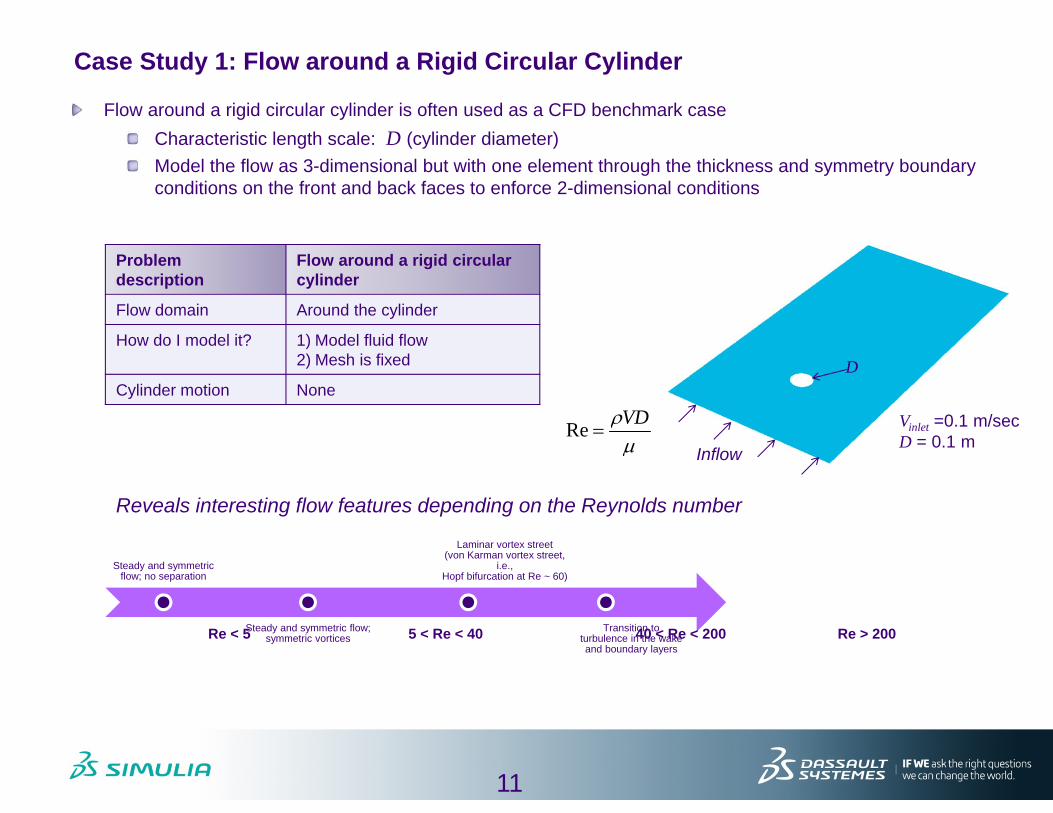
Case Study 1: Flow around a Rigid Circular Cylinder
Flow around a rigid circular cylinder is often used as a CFD benchmark caseCharacteristic length scale: D (cylinder diameter)Model the flow as 3-dimensional but with one element through the thickness and symmetry boundary conditions on the front and back faces to enforce 2-dimensional conditions
Steady and symmetric flow; no separation
Steady and symmetric flow; symmetric vortices
Laminar vortex street (von Karman vortex street,
i.e., Hopf bifurcation at Re ~ 60)
Transition to turbulence in the wake and boundary layers
Re < 5 5 < Re < 40 40 < Re < 200 Re > 200
InflowRe VD
D
Vinlet =0.1 m/secD = 0.1 m
Reveals interesting flow features depending on the Reynolds number
Problemdescription
Flow around a rigid circularcylinder
Flow domain Around the cylinder
How do I model it? 1) Model fluid flow2) Mesh is fixed
Cylinder motion None

12
Case Study 1: Defining the CFD Model
1. Create a “CFD” model in Abaqus/CAE
CFD-specific model attributes are only accessible for Abaqus/CAE models of type “CFD”The model type, once set, cannot be changed
Parts, instances, material properties etc. can be copied between “Standard & Explicit” and “CFD” model types

13
Case Study 1: Defining the CFD Model
Only 3-dimensional parts can be modeled.Use a 3D sector for axisymmetric models Use a 3D part with one element through the thickness for 2-dimensional models
Orphan CFD meshes can be importedTetrahedral and hexahedral elements only
All Abaqus/CAE features for geometry creation are accessible
“2-dimensional”D4D
4D
12D
Far field boundaries are chosen such that flow is unaffected by the presence of the cylinder at these boundaries
2. Define a part representing the flow domain

14
Case Study 1: Defining the CFD Model
Hexahedral (FC3D8), tetrahedral (FC3D4) and wedge (FC3D6) element types are available
Mixed meshes are allowedTetrahedral + WedgeHexahedral + Wedge
Proper modeling of the boundary layer requires a fine mesh near the cylinder surface to resolve the velocity gradient
Fluid velocity is zero at the cylinder surface (no-slip, no-penetration condition)Typically, the CFD mesh is refined at no-slip walls and coarsens as we move away from walls
3. Generate the mesh

15
Case Study 1: Defining the CFD Model
Newtonian fluid Density: 1000 kg/m3
Viscosity: 0.1 kg/m/sProperties are chosen to set the flow Reynolds number at 100 based on cylinder diameter
4. Define fluid material properties

16
Case Study 1: Defining the CFD Model
Section category “Fluid” is the only choice available when the CFD model type is chosenElements without a section assignment will cause a processing error
Instance the part (or orphan mesh) and position it in the desired geometric location
5. Create and assign a fluid section and instance the part

17
Case Study 1: Defining the CFD Model
Transient analysis attributesTime periodEnergy equation (off by default)Time incrementation (automatic or fixed)Solver controlsLaminar or turbulent flows
Enable heat transferAnalysis time period
6. Define an incompressible flow analysis

18
Case Study 1: Defining the CFD Model
CFL limit: Courant-Fredrichs-Levy (CFL) conditionArises due to the explicit treatment of advective terms in the Navier-Stokes equations
Time integration accuracy• 2nd order accuracy for trapezoid scheme
Automatic time integration parameters• Initial time increment• CFL limit
Time increment growth
Time incrementation
Automatic and fixed time incrementation
Controls pressure update
6. Define an incompressible flow analysis (cont’d)

19
Case Study 1: Defining the CFD Model
Primary solution quantitiesVelocity componentsPressure
Convergence and diagnostic output for each of the equations is not written by default, but they can be toggled onMany solver choices are available for the Pressure Poisson’s Equation
Use preset levels (default 2)
Momentum Equation Pressure Equation
Solver controls
6. Define an incompressible flow analysis (cont’d)

20
Case Study 1: Defining the CFD Model
Laminar or turbulent flowLaminar flow (default)Choice of turbulence models
6. Define an incompressible flow analysis (cont’d)

21
Case Study 1: Defining the CFD Model
Output frequency
Flow field output variables are available at nodes
7. Request output variables

22
Case Study 1: Defining the CFD Model
One element in the thickness direction Symmetry boundary conditions on faces to enforce 2-dimensional conditions
Reynolds number = 100
Flow outletp = 0
Flow inletVx = 0.1Vy = 0 Vz = 0
Wall (no-slip, no-penetration)Vx = 0 Vy = 0 Vz = 0
Far fieldVx = 0.1 Vy = 0 Vz = 0
Symmetry Vz = 0
Fluid boundary conditions are applied on surfaces
8. Define boundary conditions

23
Case Study 1: Defining the CFD Model
Flow inlet
Flow outlet
8. Define boundary conditions (cont’d)

24
Case Study 1: Defining the CFD Model
Wall condition Far field velocities Symmetry at front and back faces
8. Define boundary conditions (cont’d)

25
Case Study 1: Analysis Execution
Job execution optionsInput file writingAnalysis data checkJob submissionJob monitoringAccessing output database (ODB)Job termination
CFD analysis job

26
Case Study 1: Postprocessing Results
Turn off mesh display
Use continuous contour intervals
3. Fast view manipulation
(for large CFD models)
Abaqus/Viewer – Tips for postprocessing CFD output databases
3
2
2
11

27
Case Study 1: Postprocessing Results
Velocitycontour
Pressurecontour
Vorticityanimation
Contour plots & animations

3DS.
COM/
SIMU
LIA©
Das
sault
Sys
tèmes
| ref.
: 3DS
_Doc
umen
t_201
2
Modeling Heat Transfer

29
Modeling Heat Transfer: Introduction
Flow around an oscillating rigid circular cylinderCylinder surface is now at an elevated temperature while the incoming flow is cooler
What do I need to model heat transfer?
Vinlet =0.1 m/secD = 0.1 mAo = 0.05 mTp = 2 sec initial = 283 K
Inflow
D
= 283 K
= 313 K
Fluid thermal properties
Specific heat
Thermal conductivity
Enable heat transfer
Linear solver for transport equation
Define thermal boundary conditions and initial conditions
Temperature at boundaries
Initial temperature
Relevant output quantities
Temperature

30
Modeling Heat Transfer: Defining the CFD Model
1. Define thermal properties
Thermal Conductivity Specific heat at constant pressurecp is required for incompressible flow analyses
31
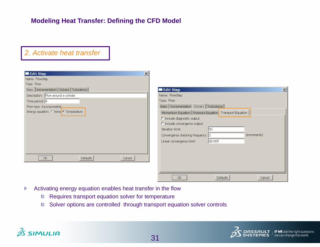
Modeling Heat Transfer: Defining the CFD Model
Activating energy equation enables heat transfer in the flow Requires transport equation solver for temperatureSolver options are controlled through transport equation solver controls
2. Activate heat transfer

32
Modeling Heat Transfer: Defining the CFD Model
Additional boundary conditions for temperatureFlow inlet Cylinder surface
3. Define boundary conditions
Define inlet temperature Define cylinder surface temperature

33
Modeling Heat Transfer: Defining the CFD Model
Solution of a transient flow problem requires initial conditionsZero initial velocity is assumed unless non-zero initial velocities are specifiedIncluding thermal effects, however, requires specification of initial temperature
4. Define initial conditions
initial = 283 K
34
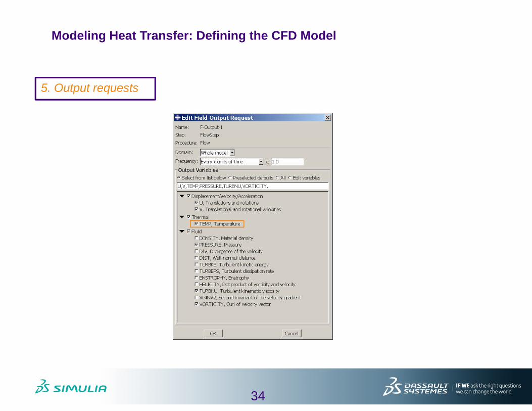
Modeling Heat Transfer: Defining the CFD Model
5. Output requests
35
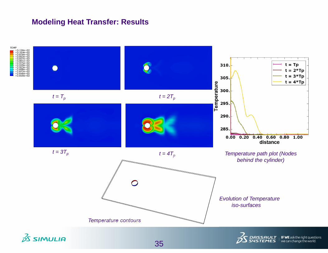
Modeling Heat Transfer: Results
Temperature contours
t = Tp t = 2Tp
t = 3Tp t = 4Tp Temperature path plot (Nodes behind the cylinder)
Evolution of Temperature iso-surfaces

3DS.
COM/
SIMU
LIA©
Das
sault
Sys
tèmes
| ref.
: 3DS
_Doc
umen
t_201
2
Modeling Turbulence

37
Modeling Turbulence: Introduction
Many CFD problems are laminar, and/or can be adequately resolved with reasonable mesh sizes, and do not require the use of a turbulence model
For problems that are truly laminar, use of a turbulence model may yield incorrect results that are too dissipative
Before activating a turbulence model, check the Reynolds number for the flowA very large Reynolds number typically indicates the need for a turbulence model
The transition Reynolds number depends on the flow itself, for example: I. For pipe flows: transition Re ~2300II. For flow around a rigid circular cylinder: transition Re ~200
If you are unsure, try this test:1. Run the simulation without a turbulence
model activated2. Plot kinetic energy and/or the time-history of
several flow variables
3. If there are random oscillations in the results, rerun the simulation with a turbulence model activated to achieve desiredsolution
Time
Velo
city
Time
Velo
city
Steady laminar flow Unsteady laminar flow
Time
Velo
city
Time
Velo
city
Steady turbulent flow Unsteady turbulent flow

38
Modeling Turbulence: Introduction
Consider the case of flow around an oscillating rigid circular cylinder that is maintained at an elevated temperature
But the Reynolds number is now 1000 for the stationary cylinder Turbulent flow regime
What do I need to model turbulent flow?
Vinlet = 0.1 m/sec= 1.0 m/sec
D = 0.1 mAo = 0.05 mTp = 2 secinitial = 283 K
Inflow
D
= 283 K
= 313 K
Select turbulence model
Linear solvers for transport equations for turbulence quantities
Define boundary conditions and initial conditions for
turbulence quantities
Dependent on turbulence model
Relevant output quantities
Dependent on turbulence model
Re 1000

39
Modeling Turbulence: Defining the CFD Model
Turbulence model parameters are characteristic of turbulence modelsTurbulence variables that are solved for depend on particular turbulence model chosen
Requires transport equation solver for turbulence variablesSolver options are controlled through transport equation solver controls
1. Activate turbulence model

40
Modeling Turbulence: Defining the CFD Model
Boundary conditions for turbulence modelsSpalart-Allmaras turbulence model requires specification of a modified turbulent kinematic viscosityAdditionally, the distance from walls needs to be evaluated
2. Boundary conditions
Automatically set by Abaqus/CAE at surfaces where no-slip or shear wall condition is applied
Walls Inlet
Inlet turbulence specification
/
3 5
...kinematic viscosity
At walls :At inlet :Inlet turbulence ( )
00d

41
Modeling Turbulence: Defining the CFD Model
Initial conditions are required for turbulence variablesThe Spalart-Allmaras turbulence model requires specification of the initial eddy viscosityIt is typically specified using the same rules for the inlet/free-stream values:
3. Initial conditions
3 5t

42
Modeling Turbulence: Defining the CFD Model
4. Output requests
Distance function output – Distance from walls
Turbulent kinematic viscosity t

43
Modeling Turbulence: Results
Turbulent eddy viscosity

3DS.
COM/
SIMU
LIA©
Das
sault
Sys
tèmes
| ref.
: 3DS
_Doc
umen
t_201
2
Native FSI

45
Native FSI using Abaqus
Fluid-structure interactionButterfly valve
Conjugate heat transferHeat exchanger
Coupling Abaqus/Standard + Abaqus/CFD
Abaqus/Explicit + Abaqus/CFD
Fluid structure interaction
Conjugate heat-transfer

46
Native FSI using Abaqus
Abaqus/CFD couples with both Abaqus/Standard and Abaqus/Explicit through the co-simulation engine
The co-simulation engine operates in the background (no user intervention required)
Physics-based conservative mapping on the FSI interface
Significantly expands the set of FSI applications that SIMULIA can address
Fluid-structure interaction
Also supports conjugate heat-transfer applications
Abaqus/Standard
Co-Simulation
Abaqus/Explicit
Abaqus/CFD

3DS.
COM/
SIMU
LIA©
Das
sault
Sys
tèmes
| ref.
: 3DS
_Doc
umen
t_201
2
FSI Simulation Workflow

48
Setting up FSI Analyses
Case study summary1. Flow around a rigid circular cylinder2. Flow around a spring-loaded rigid circular cylinder
Problemdescription
Flow around a rigid circularcylinder
Flow around a spring-loaded rigid circular cylinder
Flow domain Around the cylinder Around the cylinder but domain changes due to cylinder’s oscillation
How do I model it?
1)Model fluid flow2)Mesh is fixed
1)Model fluid flow2)Allow mesh at cylinder surface to
accommodate displacements (ALE)3)Model the cylinder and the spring in
structural solver (co-simulation)
Cylinder motion
None Determined by structural analysis(two separate models)

3DS.
COM/
SIMU
LIA©
Das
sault
Sys
tèmes
| ref.
: 3DS
_Doc
umen
t_201
2
Setting up FSI Analysis

50
Case Study 3: Flow around a Spring-loaded Rigid Circular Cylinder
Consider the case of flow around a spring-loaded rigid circular cylinderFlow at Reynolds number = 100
Boundary motion due to structural deformationThe structural deformation and fluid velocities are governed by the coupled physicsBoundary conditions on the mesh displacements and fluid velocities are dictated by the structural deformation
Vinlet = 0.1 m/secD = 0.1 m
Inflow
D
Spring-loaded rigid cylinder
Fluid StructureForce
Displacement, Velocity

51
Case Study 3: Defining the CFD Model
Wall (no-slip, no-penetration)
Flow outletp = 0
Flow inletVx = 0.1Vy = 0Vz = 0
Far fieldVx = 0.1Vy = 0Vz = 0
Symmetry Vz = 0
1. Define boundary conditions
FSI kinematic conditions require that the displacements and velocities at the FSI interface match
The co-simulation interface is used to define fluid-structure interaction and kinematic constraints
Suppress the wall BC on the cylinder surface
52
Case Study 3: Defining the CFD Model
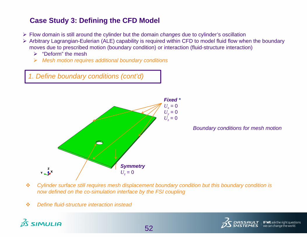
1. Define boundary conditions (cont’d)
Boundary conditions for mesh motion
SymmetryUz = 0
Fixed *Ux = 0Uy = 0Uz = 0
Cylinder surface still requires mesh displacement boundary condition but this boundary condition is now defined on the co-simulation interface by the FSI coupling
Define fluid-structure interaction instead
Flow domain is still around the cylinder but the domain changes due to cylinder’s oscillation Arbitrary Lagrangian-Eulerian (ALE) capability is required within CFD to model fluid flow when the boundary
moves due to prescribed motion (boundary condition) or interaction (fluid-structure interaction) “Deform” the mesh Mesh motion requires additional boundary conditions

53
Case Study 3: Defining the CFD Model
Boundary conditions for mesh motion
Fixed mesh Symmetry
2. Define boundary conditions (cont’d)

54
Case Study 3: Defining the CFD Model
The interaction surface needs to be definedOnly one surface per co-simulation definition*
Only one FSI co-simulation definition per analysis step
3. Define fluid-structure interaction
Define fluid-interaction surface
* If necessary, multiple surfaces can be merged into a single surface

55
Case Study 3: Defining the CFD Model
3. Define fluid-structure interaction (cont’d)
The displacements and velocities that are imported into Abaqus/CFD from Abaqus/Standard or Abaqus/Explicit serve as prescribed boundary conditions for Abaqus/CFD at the FSI interface
Fluid StructureForce
DisplacementVelocity
Abaqus/Standard +
Abaqus/CFD
Abaqus/Explicit +
Abaqus/CFD
Option Abaqus/Standard
Abaqus/CFD
Abaqus/Explicit
Abaqus/CFD
Fluid-structure
interaction
Export DisplacementVelocity
Forces DisplacementVelocity
Forces
Import Forces DisplacementVelocity
Forces DisplacementVelocity

56
Case Study 3: Defining the Structural Model
The FSI interface in the structural and CFD models should be co-located
Fixed at ground (U = 0)
Axial Connector definitionDefines a spring with linear stiffness, K = 1 N/m
Rigid cylinderThe cylinder is constrained to move in the axial flow direction

57
Case Study 3: Defining the Structural Model
Define fluid-structure interaction
The interaction surface needs to be definedOnly one surface per co-simulation definition*
Only one FSI co-simulation definition per analysis step can be defined
Define fluid-interaction surface
* If necessary, multiple surfaces can be merged into a single surface

58
Case Study 3: FSI Analysis Execution
Coupled fluid-structure interaction jobs can be set up and run interactively using the co-execution framework in Abaqus/CAE
Creating co-execution jobs
Define structural jobDefine CFD job
Automatically chosenbased on selected models

59
Case Study 3: Postprocessing FSI Analyses
Open the structural and CFD output databases simultaneously Can also overlay viewports from multiple output databases
Cylinder displacementPressure contours

3DS.
COM/
SIMU
LIA©
Das
sault
Sys
tèmes
| ref.
: 3DS
_Doc
umen
t_201
2
FSI Analysis with Shells/Membranes

61
FSI Analyses with Shells/Membranes
Fluid-structure interaction analyses can be performed when structures are modeled with shells/membranes
Recommended in cases when modeling thin structures
Alleviates small element sizes in the surrounding CFD modelImproves time increment sizes
FSI analyses require
Zero-thickness shells in CFD domain“Seam” in the CFD mesh
Define positive & negative surfaces (SPOS & SNEG, respectively) for defining fluid-structure interaction interface
CFD Mesh
Shell structure“Seam”

62
FSI Analyses with Shells/Membranes
Creating a seam in a CFD meshRequires use of the Crack feature in Abaqus/CAE
Available in Interaction module
Create the seamSelect internal surfaces and “Assign Seam”
Mesh the part
Proceed with the CFD model setup
Partition representing the seam
1
2
3

63
FSI Analyses with Shells/Membranes
Creating FSI surfaces
Pick the surfaces associated with the seam
Create separate positive and negative (SPOS, SNEG) shell surfacesTwo-sided shell surfaces are not supported for co-simulation
Only one surface per co-simulation definition can be definedMerge individual shell surfaces
3
2
1

3DS.
COM/
SIMU
LIA©
Das
sault
Sys
tèmes
| ref.
: 3DS
_Doc
umen
t_201
2
Conjugate Heat Transfer

65
Conjugate Heat Transfer Analyses: Introduction
Model heat transfer within a solid region that interacts with the surrounding fluidWe will show a simple example to demonstrate the basic concepts involved
Transient conjugate heat transfer between a printed cicuit board (PCB)-mounted electronic component and ambient airSpecified power dissipation within the component
Heat transfer mechanism involvedHeat transfer within the component and the PCB due to conduction – Modeled in Abaqus/StandardHeated surface of the PCB/Component induces a temperature-dependent density differential in the surrounding air
Buoyancy-driven natural convection is set upModeled in Abaqus/CFD
Component
PCB

66
Conjugate Heat Transfer Analyses: Defining the CFD Model
CFD mesh is built around the PCB/ComponentMaterial properties for air
Density: 1.127 kg/m3
Viscosity: 1.983x10⁵ kg/m/sThermal conductivity: 2.71x10² W/m/KSpecific heat (Cp): 1006.4 J/kg/KThermal expansion coefficient: 3.43x10³ /KReference temperature: 293 K
Thermal expansion property for air has been specified to enable coupling between momentum and energy equations – Natural convection
Define thermal initial condition Initial temperature of air = 293 K
Define gravity load
g
67
Conjugate Heat Transfer Analyses: Defining the CFD Model
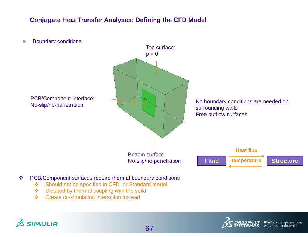
Boundary conditions
Bottom surface:No-slip/no-penetration
Top surface:p = 0
PCB/Component interface:No-slip/no-penetration
PCB/Component surfaces require thermal boundary conditions Should not be specified in CFD or Standard model Dictated by thermal coupling with the solid Create co-simulation interaction instead
No boundary conditions are needed on surrounding wallsFree outflow surfaces
Fluid Structure
Heat flux
Temperature

68
Abaqus/Standard +
Abaqus/CFD
Abaqus/Explicit +
Abaqus/CFD
Coupling type Option Abaqus/Standard
Abaqus/CFD Abaqus/Explicit Abaqus/CFD
Conjugate heat transfer
Export Temperature Heat flux Temperature Heat flux
Import Heat flux Temperature Heat flux Temperature
Conjugate Heat Transfer Analyses: Defining the CFD Model
Define thermal interaction
The co-simulation definition enables thermal coupling between the fluid and the structure
Fluid Structure
Heat flux
Temperature

69
Conjugate Heat Transfer Analyses: Defining the Structural Model
Printed circuit board (PCB)-mounted electronic componentHeat transfer step in Abaqus/Standard
Density(Kg/m3)
Specific heat(J/Kg/K)
Thermal conductivity
(W/m/K)
Thermal expansion
(/K)
PCB substrate 8950 1300 19.25 1.6 × 10⁵
Encapsulant 1820 882 0.63 1.9 × 10⁵
Die 2330 712 130.1 3.3 × 10⁶
Heat slug 8940 385 398 3.3 × 10⁶

70
Conjugate Heat Transfer Analyses: Defining the Structural Model
Define thermal interaction

71
Conjugate Heat Transfer Analyses: Results
PCB/Component:Temperature contours
Surrounding air:Temperature and velocity contours

72
Abaqus/CFD 6.13 New Features
Steady state SolverHybrid FE/FV SIMPLE
New Pyramid ElementTet-to-brick transition, tet-to-tet transition
Turbulence ModelsNew RANS model - SST variant of k-Hybrid wall function
Heat TransferRadiation and film boundary conditionsConduction heat transfer within CFD
ALE Mesh MotionA new mesh smoother based on an implicit algorithm using a “matrix-free” method

3DS.
COM/
SIMU
LIA©
Das
sault
Sys
tèmes
| ref.
: 3DS
_Doc
umen
t_201
2