multiphysical modeling of dc and ac electroosmosis in...

26

Multiphysical Modeling of DC and AC Electroosmosis in Micro- and Nanosystems

Michal Přibyl, Dalimil Šnita and Miloš Marek Institute of Chemical Technology, Prague

Czech Republic

1. Introduction

A large family of microfluidic devices employs the electrokinetic transport of liquids. The integration of mechanical components such as high-pressure pumps or valves is not required in the electrokinetically driven microfluidic chips. Instead of a pressure gradient, a gradient of electric potential is imposed over the microfluidic system. It can be provided by either DC or AC electric field. The DC electroosmotic transport in microchannels has been intensively theoretically and experimentally studied. The origin of the DC electroosmosis arises from the coulombic interaction between an external DC electric field and a mobile electric charge localized at an electrolyte-dielectric interface. The use of the electroosmosis forced by a low amplitude AC electric field is a novel area investigated only for several years. The AC electroosmosis is mostly based on the coulombic interaction between an imposed AC electric field and a mobile electric charge temporally arising at electrolyte-metal electrode interfaces. The chapter is organized as follows. The origin of the electrokinetic transport and the principle of DC and AC electroosmotic micropumps are shortly described in the first section. The basic features of the AC micropumps are summarized in more detail. The multiphysical model of electro-microfluidic systems based on the Poisson-Nernst-Planck-Navier-Stokes approach and its possible simplifications are briefly described in the second section. The implementation procedure of this multiphysical problem in a CFD software and frequently arising problems are discussed in the next section. Various electro-microfluidic systems have been investigated in our research group. Here, we present and discuss selected results of the numerical analysis of three particular micro- and nano-fluidic systems: (i) a tubular microfluidic sensor for heterogeneous immunoassay driven by a DC electric field, (ii) a submicron channel/pore interacting with a DC electric field and the surrounding electrolyte, (iii) AC electrokinetic micro- and nano-pumps realized in channels with spatially periodic arrays of co-planar electrodes. The discussed AC pumps rely either on the asymmetric geometry of interdigital electrodes or on an electric field phase shift applied to electrodes (the three phase arrangement).

1.1 Origin of Electroosmotic Transport

The electroosmotic transport can be induced by an external electric field in fluidic systems where the electric polarization (charging) of solid surfaces occurs. Some organic

www.intechopen.com

Recent Advances in Modelling and Simulation

502

(polystyrene, plexiglass) or inorganic polymers (glass) gain a surface electric charge if immersed in an electrolyte. The fixed charge can arise, e.g., from dissociation of surface chemical groups of either the polymer substrate itself or of adsorbed additives. Counterions are attracted to the charged solid phase via the coulombic force and the electric double layer (EDL) is formed. In the immediate proximity, the counterions are tightly bound to the charged surface and thus become immobile. This thin part of EDL is called the Stern layer. Further away from the solid phase in the diffusive part of EDL, the attraction coulombic force is relatively weak and the counterions remain mobile. The diffusive layer is usually much wider than the Stern layer. The imaginary surface between the diffusive and the Stern layers is called the outer Helmhotz plane – OHP, Fig. 1(A). The electric potential localized on this surface and related to the reference potential value in the bulk solution (Φ0) is an important characteristic of EDL, so-called zeta-potential ( )ζ . Let us note that the EDL

structure depicted in Fig. 1 represents a typical steady state that is established when: (i) the dielectric or the electrode surface is in a contact with the electrolyte for a long time, (ii) any temperature changes and bulk concentration changes do not occur in space and time, and (iii) the electrolyte does not move. These conditions are often not satisfied in real applications and thus the EDL structure can be more complex. However, the idea of the steady state EDL is good enough for a basic introduction of the problems studied below.

Figure 1. (A) Structure of electric double layer. (B) Properties of electric double layer

For aqueous electrolytes, the EDL width is typically in the range 1 nm – 1µm. The EDL width is approximately equal to the Debye length λD. For a symmetric uni-univalent electrolyte, the Debye length can be estimated as

( ),22

0FcRTD ελ = (1)

where the symbols R, T, c0, and F denote the molar gas constant, temperature, the electrolyte concentration in the bulk, and Faraday’s constant, respectively. The permittivity of the

www.intechopen.com


503

environment ε is equal to the product of the vacuum permittivity ε0 and the dielectric constant (relative permittivity) of the environment εr. The fixed electric charge on the solid phase is usually negative (depends on the substrate and the electrolyte pH value). Then, the electric potential decreases from the electrolyte bulk to the solid surface. In the same direction, the anion concentration decreases and the cation concentration increases with respect to the bulk concentration. Hence, the electrolyte in the EDL region does not satisfy the electroneutrality condition, i.e., a nonzero concentration of a mobile electric charge exists in EDL, Fig. 1(B). More information about EDL and electrohydrodynamic phenomena can be found, e.g., in (Probstein, 1994, Squires & Bazant, 2004, Squires & Quake, 2005).

1.2 DC Pumps

The most common feature of the DC electroosmotic micropumps is the fact that the systems work either in or close to a hydrodynamic steady state. The principle of these devices is depicted in Fig. 2. If a DC electric field is applied in the direction tangential to the solid surface, the electric body force acts on the clouds of the mobile electric charge in the diffusive part of EDL. The vector of the local body force can be expressed as

E,f qE = (2)

where q and E are the volume concentration of the mobile electric charge and the vector of the electric field strength, respectively, defined by

,,czFqi

ii Φ−∇≡≡ ∑ E (3)

where the symbols zi, ci, and ∇Φ denote the charge number of the ith ion, the volume concentration of the ith ion, and the gradient of electric potential, respectively.

Figure 2. Principle of DC electroosmosis in a microchannel

The mobile electric charge is represented by ionic particles. As the mobile ions are forced to move via the coulombic body force, they act on the ambient liquid by viscous forces. The liquid in EDL starts to flow and induces the movement of the electrolyte body. In the steady state when the distribution of the surface electric charge is homogeneous, the velocity vector has the same direction as the tangential component of electric field strength. The velocity

www.intechopen.com


504

profile is flat in the electrolyte body where the velocity attains its maximal value, i.e., the slip velocity. In the diffusive part of EDL, the velocity gradually decreases to zero at the outer Helmholtz plane. The slip velocity vt tangential to the solid surface can be estimated from the Helmholtz-Smoluchowski equation

,tt Evη

εζ−= (4)

where ζ, η, and Et are the zeta-potential, the dynamic viscosity of the electrolyte, and the tangential component of the electric field strength, respectively. The DC electroosmotic pumps are widely exploited in experimental and commercial microfluidic devices, e.g., see reviews (Becker & Locascio, 2002, Beebe et al., 2002, Bilitewski et al., 2003, Chang & Yang, 2007, Laser & Santiago, 2004). The reaction transport processes in such devices have been also modeled and analyzed, e.g., (Erickson, 2005, He & Hauan, 2006, Postler et al., 2008). The DC devices suffer from a serious disadvantage: the potential difference imposed on microdevices usually has to be in the order of kilovolts. It results, e.g., in an undesirable bubble formation or an electrolyte contamination due to faradaic interactions on the source electrodes. This particular problem can be eliminated in the electroosmotic AC pumps.

1.3 AC Pumps

Ramos et al. was the first to study the effects of a low amplitude AC electric field imposed on co-planar electrodes in a microchannel filled by an electrolyte (Ramos et al., 1998). They observed electrokinetic transport of a new kind above the source electrodes up to frequency 500 kHz. In 2000, Ajdari proposed a design of the AC electrokinec micropumps based on arrays of asymmetric pairs of co-planar microelectrodes (Ajdari, 2000). It has been expected that the asymmetry of electric field will lead to a net flow of the electrolyte. His predictions were verified by several experimental and theoretical works (Campisi et al., 2005, Garcia-Sanchez et al., 2006, Green et al., 2002, Mpholo et al., 2003, Studer et al., 2004, Zhang et al., 2006). In general, the authors used microelectrodes with characteristic dimensions ranging from micrometers to tens of micrometers. The observed velocity of the net flow typically attained few hundreds of microns per second.

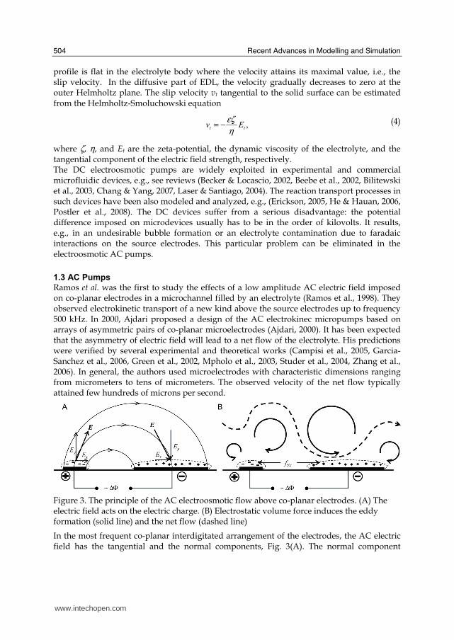
Figure 3. The principle of the AC electroosmotic flow above co-planar electrodes. (A) The electric field acts on the electric charge. (B) Electrostatic volume force induces the eddy formation (solid line) and the net flow (dashed line)

In the most frequent co-planar interdigitated arrangement of the electrodes, the AC electric field has the tangential and the normal components, Fig. 3(A). The normal component

www.intechopen.com


505

induces electrode polarization via coulombic force (capacitive charging). Then, the tangential component of the electric field forces the accumulated electric charge to move along the electrodes. The highest tangential coulombic force was predicted and observed at the electrode edges (Green et al., 2000). As the electric charge is formed by ions of a nonzero diameter, the moving ionic particles pull the surrounding liquid via viscous forces, Fig. 3(B). The combination of coulombic, pressure and viscous forces in the liquid result in the formation of eddies above the electrodes. This has been experimentally proved by the PIV technique (Garcia-Sanchez et al., 2006, Green et al., 2002). The velocity of the net flow strongly depends on several parameters: the frequency and the amplitude of the imposed electric field, the concentration of the used electrolyte and the geometric properties of the microfluidic system. The frequency dependence is given by characteristic rates of two transport processes: (i) the rate of the electrode polarization (the formation of the EDL) and (ii) the rate/frequency of an AC electric field. There are three qualitatively different regimes that can arise above the electrodes. For very low AC frequencies, the nonzero tangential coulombic force is restricted only to the electrode edges due to a complete capacitive charging of the electrodes. The force on one side of an electrode equilibrates the force on the other side and thus the net flow goes to zero. If the AC frequency is high, almost no mobile electric charge is formed at the electrode surface because the polarization process is relatively slow compared with the rate of changes of the AC electric field. As the electric field acts on zero electric charge, no net flow is induced. The AC electroosmosis can be observed between these two cases because then both a nonzero tangential component of the electric field and a nonzero mobile electric charge at the electrode surface are formed. The AC frequencies, for which the nonzero net velocity is expected, can be estimated by means of characteristic time scales of the processes inside microchannels. Let us define the following quantities

( ) ,,,221

iDDiDEACAC DDLf λτλτπτ ≡≡≡− (5)

where τAC and τE are the time scales of the AC electric field and the electrode charging, respectively. τD is the Debye time scale. The symbols fAC, L, and Di denote the AC electric field frequency, the electrode-electrode distance (alternatively the longitudinal size of electrodes), and the ionic diffusivity, respectively. There is an important difference in the physical meaning of the Debye scale and the charging scale. While the Debye time is approximately equal to the shortest time necessary for the formation of an electric charge at an electrode surface, the charging time is a typical characteristic time scale of the electrode polarization. The charging time depends on both the EDL dimension and the distance between the electrodes (Squires & Bazant, 2004). It follows from the analysis of resistor-capacitor circuits representing the AC electrokinetic systems. We can write the following condition for the value of the AC period (τAC) for which the net hydrodynamical effects are expected to be the most intensive

.EACD τττ ≈≤ (6)

The Debye time gives us a good approximation of the shortest AC period for which the net flow can be observed. The charging time estimates the typical AC period for the maximal net flow velocity.

www.intechopen.com


506

It has been found that the direction of fluid pumping is also frequency and amplitude dependent (Garcia-Sanchez et al., 2006, Studer et al., 2004). This important phenomenon has not been adequately explained yet. It is assumed that the flow reversal is caused by one or more of the following effects: (i) local salt depletion, (ii) faradaic reactions or (iii) interactions of EDL with the convective transport of ions. The transport processes related to the flow reversal are discussed in paragraph 4 in more detail. The velocity of the net flow dramatically decreases with an increasing electrolyte concentration (Studer et al., 2004). Green et al. showed that the time averaged net velocity decreases with a growing capacitance of the diffuse part of EDL (Green et al., 2002). The capacitance increases with the increasing concentration because the characteristic width of the capacitor, i.e. the Debye length, is proportional to c0-0.5 according to Eq. (1). The concentration effect on the net velocity can be a limiting factor of the use of the AC electroosmosis for the transportation of biological samples typically diluted in 10 – 100 mM buffers. There are two possible ways how to compensate the concentration effect: (i) a reduction of the electrode size, (ii) a fabrication of geometrically more complex electrodes. The former way is based on the increase of tangential electric volume force. When the amplitude of an AC field is kept constant and the electrode dimension is reduced in size, the tangential component of the electric field strength increases. The problem is that the fabrication of submicron electrodes is difficult and expensive. The latter possibility has been investigated, e.g., by (Bazant & Ben, 2006, Olesen et al., 2006, Urbanski et al., 2006). Bazant et al. predicted that a three-dimensional design of the electrodes (instead of the classical co-planar design) will increase the electrolyte net velocity up to mm s-1 (Bazant & Ben, 2006). Their theory arises from the fact that the counter-rotating regions of fluid observed above the electrode arrays inhibit the net flow, Fig. 3(B). Hence, the authors have proposed a three-dimensional electrode design where the inhibition should be negligible. It has been experimentally verified that the net velocity can be increased at least by one order of magnitude with respect to the purely co-planar arrangement (Urbanski et al., 2007, Urbanski et al., 2006). Except of the net flow forced by asymmetric interdigitated microelectrodes, the electrokinetic transport can be induced by a traveling-wave electric potential applied to an array of microelectrodes or by a spatio-temporally modulated surface potential at an insulating microchannel wall (Ejsing et al., 2006, Mortensen et al., 2005, Ramos et al., 2005). A phase shift of an AC electric field has to be provided along microchannel walls. The traveling-wave arrangement also exhibits nonlinear phenomena such as the flow reversals observed at certain AC amplitudes (Ramos et al., 2005). Different types of microfluidic pumps and mixers based on the AC faradaic electrode polarization have been proposed (Lastochkin et al., 2004). If the amplitude of an AC electric field is higher than the electrochemical limit, the electric charge on electrodes is produced via electrochemical reactions instead of the capacitive charging. The faradaic reactions do not necessary lead to gas formation. The electrode gas produced in each AC half cycle can dissolve in the electrolyte without nucleating macroscopic bubbles. For the faradaic AC micropumps are typical higher AC frequencies, AC amplitudes and electrolyte concentrations than for the capacitive charging micropumps. The net velocity attains millimeters per second. The general feature of all types of the AC electrokinetic devices is that the systems do not work in a steady state. After the initial transient, they can attain a stable periodic regime. This aspect of the AC devices substantially increases the demands on numerical analysis of

www.intechopen.com


507

model equations. From technical point of view, the most interesting velocity characteristic of the flow is the net velocity that can be obtained as the tangential velocity averaged over one period of the stable periodic regime. No comprehensive numerical study of the AC electrokinetics in microchannels has been reported. There are particularly focused studies mostly relying on the slip approximations (Kim et al., 2007, Loucaides et al., 2007) or the Poisson-Boltzmann equation (Khan & Reppert, 2005, Olesen et al., 2006, Wang & Wu, 2006, Zhang et al., 2006) but parametric studies based on mathematical models containing the full EDL description (the Poisson-Nernst-Planck-Navier-Stokes models) are rare (Mortensen et al., 2005). One can observe an interesting progress in the area of electroosmotically driven microfludic devices. Especially the DC devices have found the use in commercial bioanalytical applications. However, there are still a lot of problems to solve. The multiphysical approach to complex analysis of the transport and also the reaction processes in microfluidic chips is often missing. Linear analysis has serious limitations. Hence, robust mathematical models should be developed for a comprehensive analysis and optimization of the produced and the designed microdevices of various complexities. Below we demonstrate the use of our multiphysical mathematical model to solve selected problems related to the electroosmoticaly driven microfluidic devices. We focus on: (i) the effects of the electric charge number of antibodies and the surface electric charge on the performance of a bioassay in a tubular microchip, (ii) the analysis of strongly nonlinear dependence of the net flow velocity on AC frequency in the electroosmotic AC pumps, especially the observed flow reversals, (iii) nonlinear electrohydrodynamics and other transport phenomena in a DC single nanopore system with a fixed electric charge.

2. Mathematical Model

Nonequilibrium model of spatially distributed micro-electrochemical systems based on the mean field physical principles is formulated and discussed. We have used the following approximation: (i) systems are isothermal, (ii) the relative permittivity, the electrolyte viscosity, the electrolyte density and the ionic diffusivities are constant in each spatial domain represented by a single phase, (iii) the electrolytes are dilute and behave like Newtonian liquids, and (iv) the gravity effects are neglected.

2.1 Basic Equations and Boundary Conditions

Under the above mentioned simplifications, the velocity and the pressure fields can be computed from the Navier-Stokes equation and the continuity equation

,2vfvv

v∇+∇−=⎟⎠

⎞⎜⎝⎛

∇⋅+∂

∂ηρ p

tE

(7)

, 0=⋅∇ v (8)

where p is pressure and v is the velocity vector. According to Eq. (2), the local value of the electric body force fE depends on the distributions of the electric charge and the electric field strength E. The volume concentration of electric charge can be computed from Eq. (3) if the distributions of all ions are known. The ionic concentrations ci are evaluated using the molar balances

www.intechopen.com


508

,iiii rct

c+⋅−∇=∇⋅+

∂

∂Jv (9)

where ri is the total source of the ith component in all chemical reactions. The symbol Ji denotes the sum of the local diffusive and the local electromigration flux intensities of the the ith ionic component given by the Nernst-Planck equation

( ).RTFcDzcD iiiiii EJ +∇−= (10)

The distribution of the electric field strength or electric potential can be computed using the Poisson equation (a constant dielectric constant is considered)

εq−=Φ∇2 . (11)

The next task, and probably the most difficult one, is to find a consistent set of boundary conditions. There is no general approach how to solve this problem. The boundaries of microfluidic systems can be divided into two main groups: (i) the liquid-solid boundaries and (ii) the open boundaries. For the former group, we can, for example, use: (i) the nonslip velocity conditions, (ii) the reference pressure at a specified point (in systems with periodic boundary conditions), (iii) the normal flux of ionic components equal to zero (without chemical reactions) or the normal flux of ionic components equal to the rate of the component consumption by a surface chemical reaction (with surface chemical reactions), (iv) a specified value of electric potential (electrode surfaces, polarized dielectric surfaces) or the electric potential gradient equal to zero (electric insulator surfaces) or Gauss’s law applied on a boundary (polarized dielectric surfaces, the boundary between two dielectrics). For the latter case, we can, for example, specify: (i) the velocity profile, (ii) the reference pressure, (iii) fixed values of ionic concentrations or the Danckwerts boundary conditions (continuous flow systems), (iv) a specified value of electric potential (the potential applied on the boundary) or the electric potential gradient equal to zero (electrically insulated boundaries). The periodic boundary conditions can be applied on the open boundaries, e.g., when the system is represented by a periodic element of a microfluidic channel. In such case, it is necessary to specify the reference pressure in a single point of the system. The used sets of boundary conditions for the microfluidic systems described here can be found in (Postler et al., 2008, Pribyl et al., 2006a, Pribyl et al., 2006b). The model equations are usually transformed into a dimensionless form. The choice of the scaling factors can differ for different microfluidic systems. Examples of nondimensionalization and scaling factors can be found, e.g., in (Postler et al., 2008, Pribyl et al., 2006a, Squires & Bazant, 2004, Squires & Quake, 2005).

2.2 Model Applicability, Possible Simplifications and their Limitations

We can recognize at least two spatial scales characterizing the micro- and nanochannel systems: (i) the Debye layer scale λD, (ii) the microchannel/microelectrode scale L. Depending on the L /λD ratio, we can distinguish three different types of such systems: (i) microsystems where L >>λD, (ii) submicrosystems where L > λD, and (iii) nanosystems where L < λD. For the latter type, the use of the continuum approximation has to be cautious. In systems where the effects of a single molecule can be significant, the described mathematical model is not appropriate. The continuum approximation applied in the other

www.intechopen.com


509

two types is usually reasonable. Generally, the numerical analysis of the submicrosystems is a somewhat easier than in the analysis of the microsystems because the characteristic spatial scales are not much different. In the microsystems, the ratio of the Debye length and the characteristic width of a microchannel is typically about 10-4. The largest gradients of electric potential, ionic concentrations, velocity and pressure are usually observed in the thin Debye layer. The processes in the Debye layer affect the global behavior of microfluidic systems. Hence, in the numerical analysis of the model equations, this fact leads to substantial discretization problems connected with the increase of the problem dimension and the decrease of the computational speed. Many simplifications of the model equation were developed. One of them is based on the idea of the slip velocity. In this approach, the processes in the thin Debye layer are neglected and a nonzero tangential velocity given by Eq. (4) is considered on the interface: diffusive part of the Debye layer – the bulk solution. Thus, one of the spatial scales is eliminated. The introduction of the slip velocity also results in a substantial simplification of the model equation. If the Debye layer is an exclusive source of the nonzero mobile electric charge, the local electroneutrality is established everywhere. The right hand side of the Poisson equation is equal to zero, Eq. (11), and the distribution of electric potential is then described by the Laplacian. The electric volume force term in the Navier-Stokes equation, Eq. (7), also vanishes. Finally, the balance equations of the ionic components, Eq. (9), need not be solved. The slip velocity approach is powerful in many practical cases, e.g. (Pribyl et al., 2005); however, there are limitations. The slip velocity approach and the local electroneutrality condition should not be used, e.g., if: (i) the thickness of the Debye layer is comparable with the characteristic dimension of microfluidic channels (Pribyl et al., 2006a), (ii) an ionic component of the electrolyte interacts with a receptor bound on polarized dielectrics (Pribyl et al., 2006a), (iii) very fast chemical interactions take place (Lindner et al., 2002) etc. Another simplification assumes the Boltzmann distribution of the electric charge at the dielectric surface. It means that the microscopic velocity is low and the EDL is considered to be in the thermal equilibrium. Instead of the Poisson equation, the Poisson-Boltzmann equation (PBE) has to be solved in order to get the electric potential distribution. The PBE written for a symmetric uni-univalent electrolyte is

.sinh20

2 ε⎟⎠⎞⎜⎝

⎛ Φ=Φ∇

RT

FFc (12)

If the Boltzmann distribution is assumed, only the concentration of ions in the bulk has to be known. The molar balances of the ionic components are not solved. In some cases, the right hand side of Eq. (12) can be linearized and an exact distribution of electric potential in the EDL can be found. The linearized Eq. (12) describes the distribution with a good precision up to Φ ≈ 25 mV. The inertial forces are negligible in most microfluidic devices due to small characteristic dimensions. The nonlinear term v·∇v in Eq. (7) can be neglected and we can obtain

.2vf

v∇+∇−=

∂

∂ηρ p

tE

(13)

Further, the nonstationary term in Eq. (13) can be omitted if: (i) the flow is stationary or (ii) the flow is nonstationary but the order of the magnitude of the nonstationary term is smaller than that of the viscous term.

www.intechopen.com


510

3. Numerical Analysis

Numerical analysis of model equations can be carried out with the help of a commercial or a self-made software. In our research group, we usually employ Comsol Multiphysics software for both the stationary and the nonstationary simulations. The software is based on the finite element method and designed for various multiphysical problems. Because we mostly analyze the reaction-transport processes in the entire spatial domain including EDL, the critical step of the implementation is a proper domain discretization. The required characteristic dimension of the finite elements at polarized surfaces typically differs from the element size in the rest of the domain of a microsystem by the factor 10-4. It can be only partially resolved by the construction of a nonequidistant mesh of finite elements, e.g., a triangular mesh. While the tangential extent of the EDL is given by the dimensions of a dielectric surface, the normal extent of the EDL is approximately equal to the Debye length. It is almost impossible to construct an isotropic even if a nonequidistant mesh and not to exceed the memory capacity of a modern single CPU computer. Hence, an anisotropic (mapped) mesh of finite elements has to be constructed, e.g, a rectangular mesh. The anisotropic elements have one characteristic dimension much larger than other dimensions. Modern simulation software also enables to simply combine more types of finite element meshes on a single spatial domain. The systems described below were discretized using anisotropic or combined meshes. The elements with the highest aspect ratio were localized at the surfaces represented by polarized dielectrics or electrodes.

4. Results and Discussions

4.1 Microfluidic Biosensor

As the DC electrokinetic transport is often used in various microfluidic applications, we have decided to develop and analyze two types of mathematical models of a microfluidic biosensor. The first one is based on the physical nonslip description mentioned in the paragraph 2.1, the other one exploits the slip approximation (see the paragraph 2.2). The geometry of the microfluidic biosensor is depicted in Fig. 4. It has been considered that the microsensor is realized in a tubular microfluidic channel. Because the axial symmetry has been assumed, the reaction-transport processes have been described only in the r – z (radial-axial) coordinates and the model equation were spatially two-dimensional. The system consists of five spatial domains: (I.) the inlet compartment, (II. and IV.) the compartments with charged walls, (III.) the reaction compartment with charged or uncharged walls, (V.) the outlet compartment. The sample solution containing a ligand is introduced in the system via the boundary (1). The solution flows through all the compartments and leaves the system via the boundary (16). The ligand can bind to the receptor that is immobilized on the boundary (9), where the ligand-receptor complex is formed. In principle, the amount of the complex is proportional to the ligand concentration in the sample. We have considered that the sample is introduced in the system for a certain time period; then, an electroosmotically dosed buffer washes out the unbound ligand and the total amount of the formed complex can be detected on the boundary (9). The bioaffinity reaction scheme and the reaction parameters used in our analysis can be found in (Pribyl et al., 2006a).

www.intechopen.com


511

Figure 4. The scheme of the microfluidic sensor geometry. The roman and the arabic letters denote the domain and the boundary indexes, respectively. The width of each domain is equal to 200 µm. The height is equal to the biosensor radius, R0. The thick lines depict the DC source electrodes

The boundaries indexed in Fig. 4 can be sorted into several groups: (1, 16) – the open boundaries (the Danckwerts boundary conditions, the applied potential difference, the reference pressure), (2, 5, 8, 11, 14) – the boundaries representing the symmetry axis (the normal flux of the ionic components, the normal electric field strength and the radial velocity are equal to zero), (3, 15) – the solid uncharged boundaries (the normal flux of components, the normal electric field strength and the velocity vector are equal to zero), (4, 7, 10, 13) – the internal boundaries, (6, 12) – the solid charged boundaries at which electroosmosis is induced (the normal flux of components equal to zero, a nonzero surface electric charge, the velocity vector equal to zero or the tangential velocity equal to the slip velocity), (9) – the reaction boundary (the same as the charged boundaries except that the normal flux of the ligand is equal to the rate of the ligand consumption by a surface chemical reaction). The detailed mathematical description of both the slip and the nonslip models, their nondimensionalization and the values of the model parameters are given in the electronic supplement of (Pribyl et al., 2006a).

Figure 5. Comparison of the slip and the nonslip modeling; slip (solid line), nonslip (dotted line). (A) Dependence of the net velocity on the electrolyte concentration, R0 = 10 µm. (B) Dependence of the net velocity on the biosensor radius, c0 = 10 mol m-3

Dependence of the electroosmotic net velocity on the electrolyte concentration and the microchannel radius were computed for both models. The plots in Fig. 5. represent only an example of these dependencies found in the parametric space. Hence, the below mentioned discussion is relevant to this particular case and can not be generalized. In the slip model,

www.intechopen.com


512

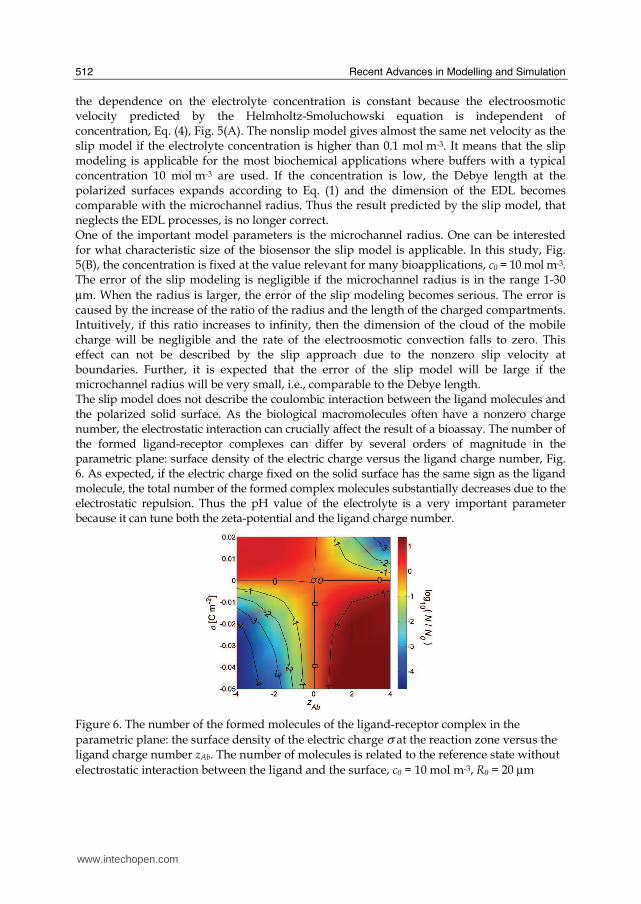
the dependence on the electrolyte concentration is constant because the electroosmotic velocity predicted by the Helmholtz-Smoluchowski equation is independent of concentration, Eq. (4), Fig. 5(A). The nonslip model gives almost the same net velocity as the slip model if the electrolyte concentration is higher than 0.1 mol m-3. It means that the slip modeling is applicable for the most biochemical applications where buffers with a typical concentration 10 mol m-3 are used. If the concentration is low, the Debye length at the polarized surfaces expands according to Eq. (1) and the dimension of the EDL becomes comparable with the microchannel radius. Thus the result predicted by the slip model, that neglects the EDL processes, is no longer correct. One of the important model parameters is the microchannel radius. One can be interested for what characteristic size of the biosensor the slip model is applicable. In this study, Fig. 5(B), the concentration is fixed at the value relevant for many bioapplications, c0 = 10 mol m-3. The error of the slip modeling is negligible if the microchannel radius is in the range 1-30 µm. When the radius is larger, the error of the slip modeling becomes serious. The error is caused by the increase of the ratio of the radius and the length of the charged compartments. Intuitively, if this ratio increases to infinity, then the dimension of the cloud of the mobile charge will be negligible and the rate of the electroosmotic convection falls to zero. This effect can not be described by the slip approach due to the nonzero slip velocity at boundaries. Further, it is expected that the error of the slip model will be large if the microchannel radius will be very small, i.e., comparable to the Debye length. The slip model does not describe the coulombic interaction between the ligand molecules and the polarized solid surface. As the biological macromolecules often have a nonzero charge number, the electrostatic interaction can crucially affect the result of a bioassay. The number of the formed ligand-receptor complexes can differ by several orders of magnitude in the parametric plane: surface density of the electric charge versus the ligand charge number, Fig. 6. As expected, if the electric charge fixed on the solid surface has the same sign as the ligand molecule, the total number of the formed complex molecules substantially decreases due to the electrostatic repulsion. Thus the pH value of the electrolyte is a very important parameter because it can tune both the zeta-potential and the ligand charge number.

Figure 6. The number of the formed molecules of the ligand-receptor complex in the parametric plane: the surface density of the electric charge σ at the reaction zone versus the ligand charge number zAb. The number of molecules is related to the reference state without electrostatic interaction between the ligand and the surface, c0 = 10 mol m-3, R0 = 20 µm

www.intechopen.com


513

4.2 Submicron Pore

Submicron channels can be found, for example, in: (i) porous ion exchange membranes, (ii) packed layers, (iii) fluidic systems with extremely thin dosing channels etc. The solid surfaces are often polarized when filled with an electrolyte. The interaction of the polarized surfaces with an external DC electric field can give rise to interesting transport phenomena because the Debye length scale and the geometric scale are comparable. From the practical point of view, the submicrochannel systems interacting with a DC electric field are exploited, e.g., in electrodialyzers. We have developed a nonequilibrium model of a single submicron pore that is filled with an electrolyte. The pore is in the contact with two surrounding electrolytes – the anolyte and the catholyte. It has been considered that the studied system consists of two phases: (i) the solid dielectric phase and (ii) the liquid electrolyte. The system can be divided into three subdomains: (i) the anolyte compartment (the electrolyte outside of the pore facing the anode), (ii) the pore compartment containing the internal electrolyte and the solid dielectrics, and (iii) the catholyte compartment (the electrolyte outside of the pore facing the cathode). The geometric domain is spatially two dimensional because we have assumed that the width of the pore is much smaller than the third spatial dimension. Another geometric simplification comes from the axial symmetry. Hence, the transport processes were studied only in one half of the pore. The schematic side view of the modeled geometry is shown in Fig. 7. We describe the left and the right open boundaries (1, 29) as the interfaces between the well mixed electrode compartments and the stagnant layers. Fixed values of the model variables are considered on the open boundaries (electric potential, pressure and concentrations). The other boundaries can be sorted into three groups: (14, 15, 19) – the electrolyte/solid interfaces with a fixed value of the surface electric charge, (2, 3, 5, 6, 8, 11, 13, 18, 21, 23, 25, 27, 28) – the boundaries representing the plane of the axial symmetry, and (4, 7, 8, 9, 10, 12, 17, 20, 22, 24, 26) – the internal boundaries used for the interfacing of structured and unstructured discretization meshes.

Figure 7. (A) The schematic view of the submicron pore geometry, (B) the domain indexes, (C) the boundary indexes. The symbol w denotes the half-width of the system that varies in the range of 1-5 Debye length units (λD)

As an illustrative example, the effect of the half-width of the system w on the current-voltage and the velocity-voltage characteristics is shown. The dependencies of the mean electric current density (averaged over the pore width) on the mean electric field strength

www.intechopen.com


514

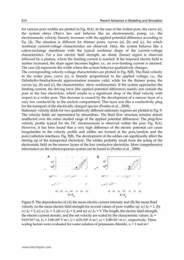
for various pore widths are plotted in Fig. 8(A). In the case of the widest pore, the curve (e), the system obeys Ohm’s law and behaves like an electroosmotic pump, i.e., the electroosmotic velocity linearly increases with the applied potential difference according to Eq. (4). The situation is different for thinner pores, curves (a), (b) and (c), for which nonlinear current-voltage characteristics are observed. Here, the system behaves like a cation-exchange membrane with the typical nonlinear shape of the current–voltage characteristics. For a low electric field strength, an ohmic (linear) region is observed followed by a plateau, where the limiting current is reached. If the imposed electric field is further increased, the slope again becomes higher; i.e., an over-limiting current is attained. The case (d) represents the width where the system behavior qualitatively changes. The corresponding velocity-voltage characteristics are plotted in Fig. 8(B). The fluid velocity in the wider pore, curve (e), is linearly proportional to the applied voltage; i.e., the Helmholtz–Smoluchowski approximation remains valid, while for the thinner pores, the curves (a), (b) and (c), the characteristics show nonlinearities. If the system approaches the limiting current, the driving force (the applied potential difference) mainly acts outside the pore in the free electrolyte, which results in a significant drop of the fluid velocity with respect to a wider pore. This decrease is caused by the development of a narrow layer of a very low conductivity in the anolyte compartment. This layer acts like a conductivity plug for the transport of the electrically charged species (Postler et al. , 2008). Stationary velocity fields for two qualitatively different stationary regimes are plotted in Fig. 9. The velocity fields are represented by streamlines. The fluid flow structure remains almost unaffected over the entire studied range of the applied potential differences. The plug-flow velocity profile typical for the DC electroosmosis is observed within the pore Fig. 9(A). However, it has been found that a very high difference of the electric potential can cause irregularities in the velocity profile and eddies are formed at the pore/anolyte and the pore/catholyte interfaces, Fig. 9(B). The development of the eddies can significantly affect the stirring up of the transported electrolyte. The eddies probably result from the acting of the electrostatic field on the narrow layers of the low conductive electrolyte. More comprehensive information on the submicroporous system can be found in (Postler et al. , 2008).

Figure 8. The dependencies of (A) the mean electric current intensity and (B) the mean fluid velocity on the mean electric field strength for several values of pore widths: (a) w/λD = 1, (b) w/λD = 2, (c) w/λD = 3, (d) w/λD = 4, and (e) w/λD = 5. The length, the electric field strength, the electric current density, and the net velocity are scaled by the characteristic values: λD = 9.63×10−9 m, E0 = 2.68×106 V m-1, i0 = 4.01×104 A m-2, u0 = 2.08×10-1 m s-1, respectively. These scaling factors were evaluated for water solution of potassium chloride, c0 = 1 mol m-3

www.intechopen.com


515

Figure 9. The velocity field, (A) E/E0 = 0.1, (B) E/E0 = 50. The pore width is w/λD = 3

4.3 AC Micropumps

AC electrokinetic micro- and nano-pumps are frequently realized in microfluidic channels using periodic arrays of co-planar electrodes. The electrode arrays are deposited on a channel wall. Mostly, a pair of asymmetric co-planar electrodes is placed in a single segment of the microchannel. In order to analyze the electroosmotic transport with the use of the nonequilibrium model, we have proposed the geometry of a single segment, Fig. 10. The single segment has been described in the cartesian coordinates. Spatially two-dimensional segment has been considered. We have assumed that the height of the channel is much smaller than the third spatial dimension of the channel, i.e., the channel profile looks like a flat rectangle. The system consists of five spatial domains: (I. and V.) the inlet/outlet compartments representing the distance between two segments of the AC pump, (II. and IV.) the compartments with the deposited electrodes, (III.) the compartment separating the electrodes. The electrolyte solution is introduced or released from the periodic segment via the open boundaries (1, 16) that are connected by the periodic boundary conditions. The boundaries (2, 3, 6, 8, 9, 12, 14, 15) represent the solid channel walls without any fixed electric charge (the normal flux of components, the surface electric charge, and the velocity vector are equal to zero). The boundaries (5) and (11) denote the electrode surfaces with an applied harmonic (sinusoidal) voltage and the reference electric potential, respectively. The zero velocity field and the zero normal flux of ionic components were considered on the electrodes. The group of the internal boundaries involves segments (4, 7, 10, 13). The reference pressure was specified only at a single point, as the single segment is not open. In this study, the amplitude of the AC electric field was equal to 1 V and the concentration of a symmetric uni-univalent electrolyte was 0.01 mol m-3. The mathematical description of the model and the other model parameters are given in (Pribyl et al., 2006b). In numerical analysis, it was necessary to compute the entire transient from the initial steady state to the stable periodic regime. The initial steady state was chosen as homogeneous in the entire segment, i.e., the zero velocity vector, the reference pressure, the reference electric potential, and the bulk concentration of the ionic components were independent of spatial coordinates. The duration of the transients depends on the AC frequency. The net velocity and the electric volume force were computed as the mean value over a single period of the stable periodic regime.

www.intechopen.com


516

Figure 10. The scheme of a single segment of the AC microfluidic pump. The roman and the arabic letters denote the domain and the boundary indexes, respectively. The widths of the domains are 10 µm, 5 µm, 2 µm, 3 µm, and 10 µm, respectively. The height is 10 µm. The thick lines depict the AC source electrodes

As mentioned in the paragraph 1.3, the net velocity of the AC electroosmotic pumping depends nonlinearly on the AC frequency. Our results also exhibit this nonlinearity, Fig. 11(A). As the AC frequency grows, one can observe two flow reversals. The net velocity is negative in the intervals ⟨1×10-1; 3×101⟩ s-1 and ⟨4×102; 1×105⟩ s-1. Positive values of the net velocity were found in the frequency interval ⟨3×101; 4×102⟩ s-1. The existence of the flow reversals is in a qualitative agreement with the published data (Garcia-Sanchez et al., 2006, Studer et al., 2004). For the given set of parameters, the maximal net velocity attains only few tens of microns per second. However, it can be substantially increased by the optimization of the geometric and the electric field parameters. If the AC frequency is low, e.g. 1×10-1 s-1, the system behaves like a condenser, i.e., the current-voltage phase shift is equal to 90 degrees, Fig. 11(B). In such regime, the electrode surfaces are fully polarized and the tangential component of the electric field strength is equal to zero except at the electrode boundaries, which results in the zero net velocity. The maximal velocity in the absolute value is observed for the AC frequency 2×103 s-1. Almost the same frequency value can be estimated from the theory as the reciprocal charging time τE , Eq. (5). The phase shift is then about 20 degrees. If the AC frequency is high, e.g., 1×10-5 s-1, the system behaves as a resistor, i.e., the current-voltage phase shift is equal to 0 degrees. The AC period is then approximately equal to the Debye time τD , Eq. (5). As no mobile electric charge can be formed at the electrode surfaces in such regime, the zero net velocity is observed.

Figure 11. Dependencies of the net velocity (A) and the current-voltage phase shift (B) on the applied AC frequency

www.intechopen.com


517

Figure 12. Dependencies of the tangential (longitudinal) component of the electric volume force on the applied AC frequency. (A) The force in each compartment and the total volume force in the entire segment, (B) the same as (A) in detail, (C) the force summed over the nonelectrode compartments, summed over the electrode compartments, and summed over the entire segment

The dependencies in Fig. 11 are strongly nonlinear. It can be helpful to study the dependence of the tangential component of the electric force ⟨FEx⟩ on the AC frequency, Fig. 12. The force has been evaluated in each segment domain as a surface integral of the tangential component of the electric volume force. The force in the nonelectrode compartments is much higher than in the electrode compartments in the AC frequency interval ⟨1×10-1; 1×103⟩ s-1. However, the sum of the electric body force over all nonelectrode compartments is always smaller (in the absolute value) than that summed over the electrode compartments, Fig. 12(C). If the AC frequency is very low, the force is localized only at the electrode-dielectric interface (the boundary interfaces 2/5, 5/8, 8/11, 11/14, see Fig. 10). Only here, the mobile electric charge and the tangential gradient of electric potential are localized together. As the transport processes are faster than the electric field alternation, the electric force is symmetric with respect to the electrode centers, i.e., the force at the 2/5 and 8/11 interfaces compensate the forces at the 5/8 and 11/14 interfaces, respectively. The phase shift is almost 90 degrees in such a regime, Fig. 11(B). In the AC frequency range ⟨1×100; 1×104⟩ s-1, the electric body force above the larger electrode (domain II.) is in the absolute value always higher than above the smaller one (domain IV.), Fig. 12(B). The dependence of the total volume force on the AC frequency has a similar shape as the velocity dependence (compare Figs. 11(A) and 12(C)). However, there are also differences: (i) the force dependence crosses zero value only once, (ii) the electric body force and the net velocity can differ in the sign at some frequencies, and (iii) the main flow reversal at fAC = 2×10-3 s-1 is not accompanied by an electric body force reversal. As expected, the dependence of the maximal amount of the electric charge QM on the AC frequency is plotted in Fig. 13(A) as a solid line. This dependence monotonically decreases with the growing frequency. In the same figure, the amount of the mobile electric charge at the time, when the applied voltage is equal to the amplitude, is plotted by the dotted line, QA. For low frequencies, these two quantities are almost the same because the electrode charging process is much faster than the electric field alternation. If the AC frequency is high, the degree of the electrode polarization is low and QA becomes smaller than QM. The

www.intechopen.com


518

ratio QA /QM is not monotonic and has a local minimum at fAC = 1×101 s-1 and a local maximum at fAC = 1×102 s-1, Fig. 13(B). If one looks on the characteristics, it can be seen that the nonlinear dependence of the net velocity can not be explained only on their bases. It will be necessary to analyze the spatial distributions of: (i) the mobile electric charge at various phases of the AC electric field, (ii) the normal component of the electric field strength, (iii) the velocity and the pressure fields, etc. At this stage, we can only conclude that the observed flow reversals do not rely on the faradaic interactions because those are not considered in our mathematical model.

Figure 13. Dependencies of the mobile electric charge in the electrode compartments on the applied AC frequency. (A) The maximal mobile electric charge during an AC period QM (solid line), the mobile electric charge if the voltage is equal to the voltage amplitude QA (dotted line), (B) the QA/QM ratio

The use of a phase shift of an AC electric field applied on a field of symmetric coplanar electrodes is an alternative to the asymmetric coplanar design. In this study, we have proposed two different realizations either with the two-phase arrangement, Fig. 14(A), or with the three-phase arrangement, Fig. 14(B). In the two-phase and the three-phase systems, the relative phase shifts 180° and 120° are applied on the adjacent electrodes, respectively. In principle, the same mathematical description as in the system depicted in Fig. 10 has been used. There are only two differences: (i) all electrodes are of the same size and (ii) the axial symmetry is assumed, i.e., the electrodes are deposited on two opposite walls.

Figure 14. The scheme of a single segment of the AC electroosmotic pump with an imposed phase shift between coplanar electrodes, (A) two-phase arrangement, (B) three-phase arrangement. The dimension of the electrodes, the dimension of the gap between the electrodes and the channel half-width are 300 λD, 50 λD, 1000 λD, respectively, (λD = 9.63×10−9 m)

www.intechopen.com


519

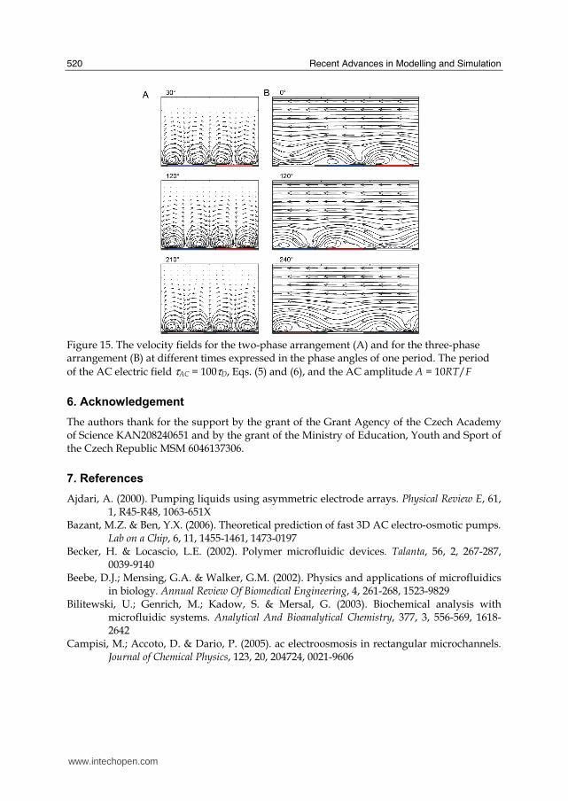
The qualitative comparison of the two-phase and the three-phase realizations is depicted in Fig. 15. For the former realization, the resulting net velocity is equal to zero because the velocity fields with 90° phase shift have the same structure but the flow direction is opposite, Fig. 15 (A). For the latter realization, one can observe a nonzero net velocity in the direction from the right to the left, Fig. 15 (B). If two velocity fields with 120° phase shift are compared, we can see that the velocity field structure is again the same, however, spatially shifted by one electrode distance (in this case to the left). The direction of the flow can be reversed if the order of phases is reversed similarly as in a three-phase electromotor.

5. Conclusion

The described Poisson-Nernst-Planck-Navier-Stokes nonequilibrium mathematical model is a powerful tool for analysis of the reaction transport processes in various microfluidic devices, namely, geometrically complex microfluidic structures with polarizable dielectric walls or deposited metal electrodes with an imposed electric potential under the electrochemical limit. The microfluidic structures have to be filled with a liquid electrolyte, no electrochemical interactions have to occur, and the applications have to be performed under isothermal conditions. For example, the proposed mathematical model enables numerical analysis of: (i) chemical and biochemical interactions in homogeneous and heterogeneous arrangement, (ii) the combined diffusion-electromigration-convective transport of ionic and electroneutral components, (iii) the DC electroosmotic convection induced at polarized surfaces, (iv) the AC electroosmotic convection forced at microelectrode arrays, (v) the pressure and the velocity fields etc. It has been demonstrated that the use of the nonequilibrium model is necessary, e.g., when the characteristic dimension of the microfluidic device is comparable with the thickness of EDL (low concentrated electrolytes, very thin microchannels) or the polarized dielectric walls interact with an ionic reaction components diluted in the electrolyte. We have shown that a porous structure surrounded by an aqueous electrolyte and affected by an external DC electric field can behave as either a DC micropump or an ionexchange membrane. The behavior depends on the pore diameter, the electrolyte concentration and other parameters. Interesting nonlinear hydrodynamic phenomena such as the eddy formation were observed in our simulations. In the future, our work will deal with the analysis of complex electrohydrodynamic processes in the pores and the surrounding electrolyte in the overlimiting current domain. It can contribute to the overlimiting current theory. Selected characteristics of the AC electroosmosis forced by the coulombic force in the studied microchannels have been presented. Both asymmetric (interdigitated) and symmetric (traveling wave) arrangements were analyzed by means of the nonequilibrium model. The obtained characteristics are nonlinear and the explanation of the flow reversals remains unclear, except the finding that the flow reversals do not necessarily rely on the electrochemical reactions. However, the model gives us the opportunity to get not only qualitative but also quantitative insights into flow reversals via detailed analysis of spatiotemporal fields of all dependent variables.

www.intechopen.com


520

Figure 15. The velocity fields for the two-phase arrangement (A) and for the three-phase arrangement (B) at different times expressed in the phase angles of one period. The period of the AC electric field τAC = 100τD, Eqs. (5) and (6), and the AC amplitude A = 10RT/F

6. Acknowledgement

The authors thank for the support by the grant of the Grant Agency of the Czech Academy of Science KAN208240651 and by the grant of the Ministry of Education, Youth and Sport of the Czech Republic MSM 6046137306.

7. References

Ajdari, A. (2000). Pumping liquids using asymmetric electrode arrays. Physical Review E, 61, 1, R45-R48, 1063-651X

Bazant, M.Z. & Ben, Y.X. (2006). Theoretical prediction of fast 3D AC electro-osmotic pumps. Lab on a Chip, 6, 11, 1455-1461, 1473-0197

Becker, H. & Locascio, L.E. (2002). Polymer microfluidic devices. Talanta, 56, 2, 267-287, 0039-9140

Beebe, D.J.; Mensing, G.A. & Walker, G.M. (2002). Physics and applications of microfluidics in biology. Annual Review Of Biomedical Engineering, 4, 261-268, 1523-9829

Bilitewski, U.; Genrich, M.; Kadow, S. & Mersal, G. (2003). Biochemical analysis with microfluidic systems. Analytical And Bioanalytical Chemistry, 377, 3, 556-569, 1618-2642

Campisi, M.; Accoto, D. & Dario, P. (2005). ac electroosmosis in rectangular microchannels. Journal of Chemical Physics, 123, 20, 204724, 0021-9606

www.intechopen.com


521

Ejsing, L.; Smistrup, K.; Pedersen, C.M.; Mortensen, N.A. & Bruus, H. (2006). Frequency response in surface-potential driven electrohydrodynamics. Physical Review E, 73, 3, 037302, 1539-3755

Erickson, D. (2005). Towards numerical prototyping of labs-on-chip: modeling for integrated microfluidic devices. Microfluidics and Nanofluidics, 1, 4, 301-318, 1613-4982

Garcia-Sanchez, P.; Ramos, A.; Green, G. & Morgan, H. (2006). Experiments on AC electrokinetic pumping of liquids using arrays of microelectrodes. Ieee Transactions on Dielectrics and Electrical Insulation, 13, 3, 670-677, 1070-9878

Green, N.G.; Ramos, A.; Gonzalez, A.; Morgan, H. & Castellanos, A. (2002). Fluid flow induced by nonuniform ac electric fields in electrolytes on microelectrodes. III. Observation of streamlines and numerical simulation. Physical Review E, 66, 2, 026305, 1063-651X

Green, N.G.; Ramos, A. & Morgan, H. (2000). Ac electrokinetics: a survey of sub-micrometre particle dynamics. Journal of Physics D-Applied Physics, 33, 6, 632-641, 0022-3727

He, X. & Hauan, S. (2006). Microfluidic modeling and design for continuous flow in electrokinetic mixing-reaction channels. Aiche Journal, 52, 11, 3842-3851,

Chang, C.C. & Yang, R.J. (2007). Electrokinetic mixing in microfluidic systems. Microfluidics and Nanofluidics, 3, 5, 501-525, 1613-4982

Khan, T. & Reppert, P.M. (2005). A finite element formulation of frequency-dependent electro-osmosis. Journal of Colloid and Interface Science, 290, 2, 574-581, 0021-9797

Kim, B.J.; Yoon, S.Y.; Sung, H.J. & Smith, C.G. (2007). Simultaneous mixing and pumping using asymmetric microelectrodes. Journal of Applied Physics, 102, 7, 074513, 0021-8979

Laser, D.J. & Santiago, J.G. (2004). A review of micropumps. Journal Of Micromechanics And Microengineering, 14, 6, R35-R64, 0960-1317

Lastochkin, D.; Zhou, R.H.; Wang, P.; Ben, Y.X. & Chang, H.C. (2004). Electrokinetic micropump and micromixer design based on ac faradaic polarization. Journal of Applied Physics, 96, 3, 1730-1733, 0021-8979

Lindner, J.; Snita, D. & Marek, M. (2002). Modelling of ionic systems with a narrow acid base boundary. Physical Chemistry Chemical Physics, 4, 8, 1348-1354, 1463-9076

Loucaides, N.; Ramos, A. & Georghiou, G.E. (2007). Novel systems for configurable AC electroosmotic pumping. Microfluidics and Nanofluidics, 3, 6, 709-714, 1613-4982

Mortensen, N.A.; Olesen, L.H.; Belmon, L. & Bruus, H. (2005). Electrohydrodynamics of binary electrolytes driven by modulated surface potentials. Physical Review E, 71, 5, 056306, 1539-3755

Mpholo, M.; Smith, C.G. & Brown, A.B.D. (2003). Low voltage plug flow pumping using anisotropic electrode arrays. Sensors and Actuators B-Chemical, 92, 3, 262-268, 0925-4005

Olesen, L.H.; Bruus, H. & Ajdari, A. (2006). ac electrokinetic micropumps: The effect of geometrical confinement, Faradaic current injection, and nonlinear surface capacitance. Physical Review E, 73, 5, 056313, 1539-3755

Postler, T.; Slouka, Z.; Svoboda, M.; Pribyl, M. & Snita, D. (2008) Parametrical studies of electroosmotic transport characteristics in submicrometer channels. Journal of Colloid and Interface Science, 320, 1, 321-332, 0021-9797

www.intechopen.com


522

Pribyl, M.; Knapkova, V.; Snita, D. & Marek, M. (2005). Analysis of reaction-transport phenomena in a microfluidic system for the detection of IgG. Chemical Papers-Chemicke Zvesti, 59, 6A, 434-440, 0366-6352

Pribyl, M.; Knapkova, V.; Snita, D. & Marek, M. (2006a). Modeling reaction-transport processes in a microcapillary biosensor for detection of human IgG. Microelectronic Engineering, 83, 4-9, 1660-1663, 0167-9317

Pribyl, M.; Schrott, W.; Shahravan, A. & Snita, D. (2006b). Mathematical modeling of a microchip driven by AC electric field, Proceedings of 2006 International Symposium on Electrohydrodynamics, pp. 309-312, CD ROM, ISBN 950-29-0964-X, Universidad de Buenos Aires, Buenos Aires

Probstein, R.F., Physicochemical hydrodynamics: An Introduction. second ed. 1994, New York: Wiley and Sons.

Ramos, A.; Morgan, H.; Green, N.G. & Castellanos, A. (1998). Ac electrokinetics: a review of forces in microelectrode structures. Journal of Physics D-Applied Physics, 31, 18, 2338-2353, 0022-3727

Ramos, A.; Morgan, H.; Green, N.G.; Gonzalez, A. & Castellanos, A. (2005). Pumping of liquids with traveling-wave electroosmosis. Journal of Applied Physics, 97, 8, 084906, 0021-8979

Squires, T.M. & Bazant, M.Z. (2004). Induced-charge electro-osmosis. Journal of Fluid Mechanics, 509, 217-252, 0022-1120

Squires, T.M. & Quake, S.R. (2005). Microfluidics: Fluid physics at the nanoliter scale. Reviews of Modern Physics, 77, 3, 977-1026, 0034-6861

Studer, V.; Pepin, A.; Chen, Y. & Ajdari, A. (2004). An integrated AC electrokinetic pump in a microfluidic loop for fast and tunable flow control. Analyst, 129, 10, 944-949, 0003-2654

Urbanski, J.P.; Levitan, J.A.; Burch, D.N.; Thorsen, T. & Bazant, M.Z. (2007). The effect of step height on the performance of three-dimensional ac electro-osmotic microfluidic pumps. Journal of Colloid and Interface Science, 309, 2, 332-341, 0021-9797

Urbanski, J.P.; Thorsen, T.; Levitan, J.A. & Bazant, M.Z. (2006). Fast AC electro-osmotic micropumps with nonplanar electrodes. Applied Physics Letters, 89, 14, 143508, 0003-6951

Wang, X.M. & Wu, J.K. (2006). Flow behavior of periodical electroosmosis in microchannel for biochips. Journal of Colloid and Interface Science, 293, 2, 483-488, 0021-9797

Zhang, Y.L.; Wong, T.N.; Yang, C. & Ooi, K.T. (2006). Dynamic aspects of electroosmotic flow. Microfluidics and Nanofluidics, 2, 3, 205-214, 1613-4982

www.intechopen.com

Modelling and SimulationEdited by Giuseppe Petrone and Giuliano Cammarata

ISBN 978-3-902613-25-7Hard cover, 688 pagesPublisher I-Tech Education and PublishingPublished online 01, June, 2008Published in print edition June, 2008

InTech EuropeUniversity Campus STeP Ri Slavka Krautzeka 83/A 51000 Rijeka, Croatia Phone: +385 (51) 770 447 Fax: +385 (51) 686 166www.intechopen.com

InTech ChinaUnit 405, Office Block, Hotel Equatorial Shanghai No.65, Yan An Road (West), Shanghai, 200040, China

Phone: +86-21-62489820 Fax: +86-21-62489821

This book collects original and innovative research studies concerning modeling and simulation of physicalsystems in a very wide range of applications, encompassing micro-electro-mechanical systems, measurementinstrumentations, catalytic reactors, biomechanical applications, biological and chemical sensors,magnetosensitive materials, silicon photonic devices, electronic devices, optical fibers, electro-microfluidicsystems, composite materials, fuel cells, indoor air-conditioning systems, active magnetic levitation systemsand more. Some of the most recent numerical techniques, as well as some of the software among the mostaccurate and sophisticated in treating complex systems, are applied in order to exhaustively contribute inknowledge advances.

How to referenceIn order to correctly reference this scholarly work, feel free to copy and paste the following:

Michal Pribyl, Dalimil Snita and Milos Marek (2008). Multiphysical Modeling of DC and AC Electroosmosis inMicro- and Nanosystems, Modelling and Simulation, Giuseppe Petrone and Giuliano Cammarata (Ed.), ISBN:978-3-902613-25-7, InTech, Available from:http://www.intechopen.com/books/modelling_and_simulation/multiphysical_modeling_of_dc_and_ac_electroosmosis_in_micro-_and_nanosystems

multiphysical modeling of dc and ac electroosmosis in...

Documents