electroosmosis and thermal effects in …digitaladdis.com/sk/vaibhav_patel_thesis_mhd.pdf ·...
TRANSCRIPT

ELECTROOSMOSIS AND THERMAL EFFECTS IN
MAGNETOHYDRODYNAMIC (MHD) MICROPUMPS USING 3D MHD
EQUATIONS
_______________
A Thesis
Presented to the
Faculty of
San Diego State University
_______________
In Partial Fulfillment
of the Requirements for the Degree
Masters of Science
in
Mechanical Engineering
_______________
by
Vaibhav D. Patel
Spring 2007

SAN DIEGO STATE UNIVERSITY
The Undersigned Faculty Committee Approves the
Thesis of Vaibhav D. Patel:
Electroosmosis and Thermal Effects in Magnetohydrodynamic (MHD)
Micropumps Using 3D MHD Equations
_____________________________________________
Samuel Kinde Kassegne, Chair
Department of Mechanical Engineering
_____________________________________________
Subrata Bhattacharjee
Department of Mechanical Engineering
_____________________________________________
Jose E Castillo
Department of Mathematics and Statistics
______________________________
Approval Date

iii
Copyright © 2007
by
Vaibhav D. Patel
All Rights Reserved

iv
DEDICATION
To my mother, father their love, encouragement and support. And to the newest
member of my family, Punya.
v
ABSTRACT OF THE THESIS
Electroosmosis and Thermal Effects in Magnetohydrodynamic
(MHD) Micropumps Using 3D MHD Equations
by
Vaibhav D. Patel
Masters of Science in Mechanical Engineering
San Diego State University, 2007
Magnetohydrodynamics (MHD) is a phenomenon observed in electrically conductive
liquid in the presence of a magnetic field where a body force called “Lorentz Force” is
produced. Based on this MHD physics, MHD micropumps are increasingly being used for
pumping biological and chemical specimens such as blood and saline buffers. This research
reports the development of generalized 3D MHD equations that govern the multiphysics of
micropumps. Based on the solution of the numerical framework developed, the thesis reports
effect such as non uniform magnetic and electric fields, Joule Heating, electroosmosis, pinch
effect and M shaped velocity profile in different flow channel geometries.

vi
TABLE OF CONTENTS
PAGE
ABSTRACT...............................................................................................................................v
LIST OF TABLES................................................................................................................. viii
LIST OF FIGURES ................................................................................................................. ix
ACKNOWLEDGEMENTS..................................................................................................... xi
CHAPTER
1 INTRODUCTION .........................................................................................................1
2 LITERATURE SURVEY..............................................................................................5
2.1 MHD Physics .................................................................................................... 5
2.2 Macro and Micro MHD Phenomenon .............................................................. 5
3 MULTI-PHYSICS OF MHD PUMP...........................................................................13
3.1 Development of 3-D Equation ........................................................................ 13
3.2 Formulation of Equations for Non-Dimensional Analysis ............................ 19
3.2.1 Problem Description .............................................................................. 19
4 PRESENTATION OF RESULTS AND DISCUSSION .............................................24
4.1 Validation of results by Non-Dimensional analysis ....................................... 24
4.1.1 Reynolds Number and Effects ............................................................... 24
4.1.2 Interaction Parameter Effects................................................................. 26
4.1.3 Electrode Length Effect (Pinch Effect).................................................. 26
4.2 MHD Micropump with Different Channel Geometry Analysis ..................... 26
4.2.1 Rectangular Channel.............................................................................. 26

vii
4.2.2 Nozzle – Diffuser Channel..................................................................... 32
4.2.3 Trapezoidal Channel .............................................................................. 38
4.2.4 Trapezoidal vs. Rectangular Channel Selection .................................... 39
5 DISCUSSION OF EO AND JOULE EFFECT ...........................................................44
5.1 Electroosmosis ................................................................................................ 44
5.2 Effect of Joule Heating and Viscosity under Temperature Changes .............. 44
6 CONCLUSION............................................................................................................50
REFERENCES ........................................................................................................................53

viii
LIST OF TABLES
PAGE
Table 1.1 A Summary of Some of the Recent MHD Micropumps Reported in the
Literature......................................................................................................................12
Table 2.1 Boundary Conditions for Generalized 3D Rectangular MHD Equations for
MHD Micro Fluidics Pumps........................................................................................16
Table 2.2. Subdomain Conditions for Generalized 3D Non-Dimensional Rectangular
MHD Equations for MHD Micro Fluidics Pumps.......................................................23
Table 2.3. Boundary Conditions for Generalized 3D Non-Dimensional Rectangular
MHD Equations for MHD Macro Fluidics Pumps ......................................................23
Table 2.4 Comparison of Flow Rate, Maximum Velocity and Lorentz’s Force in
MHD Micropumps of Trapezoidal and Rectangular Cross-Sections ..........................42

ix
LIST OF FIGURES
PAGE
Figure 1.1 Typical configuration of MHD micro pumps with a rectangular cross-
section. ...........................................................................................................................3
Figure 2.1 “M-Shaped” axial velocity profiles along the channel.............................................8
Figure 2.2 “Pinch Effect” (Pressure) at the channel wall and at the channel centerline
at entrance and exit of the electrode. .............................................................................8
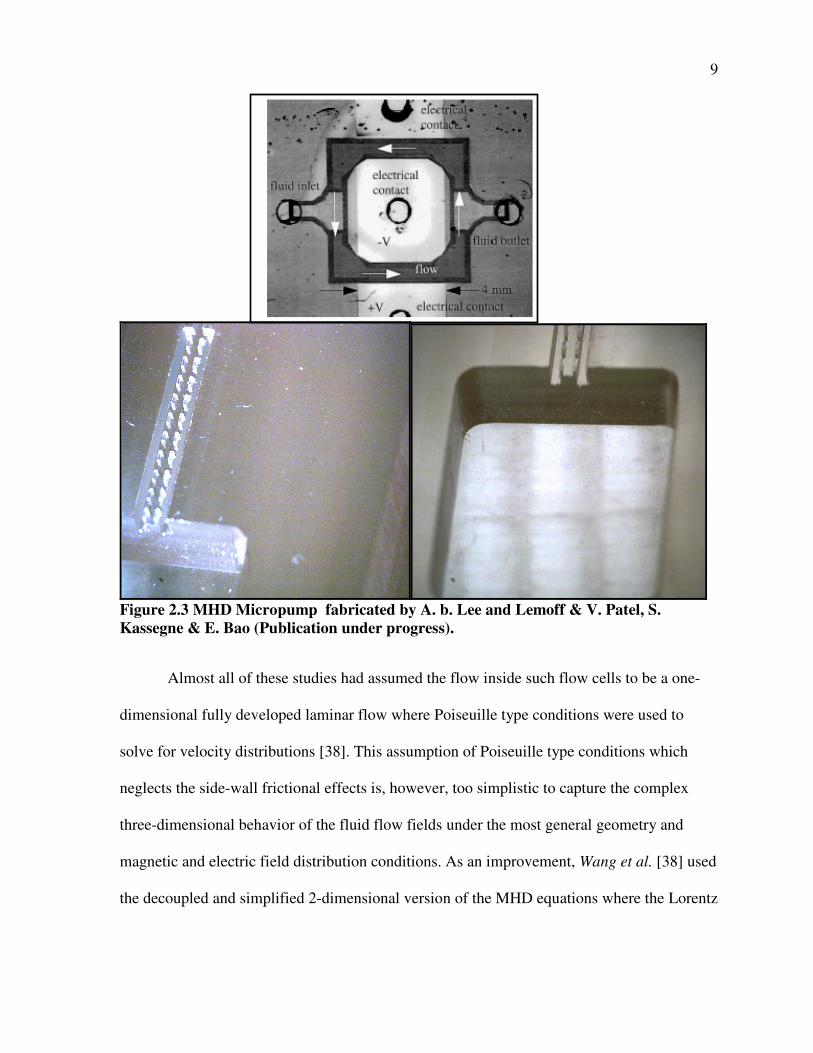
Figure 2.3 MHD Micropump fabricated by A. b. Lee and Lemoff & V. Patel, S.
Kassegne & E. Bao. .......................................................................................................9
Figure 2.4 MHD Micropump fabricated by Homsey et al.......................................................11
Figure 3.1 MHD Pump with unit dimension consideration.....................................................20
Figure 4.1 M-Shaped velocity profile along the channel line as Reynolds number
increases. ......................................................................................................................25
Figure 4.2 Pressure distribution along the MHD region with varying Re. ..............................25
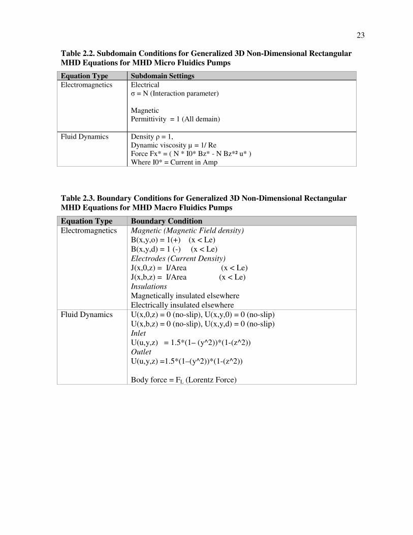
Figure 4.3 M – Shaped Profile with Varying N Interaction parameter. ..................................27
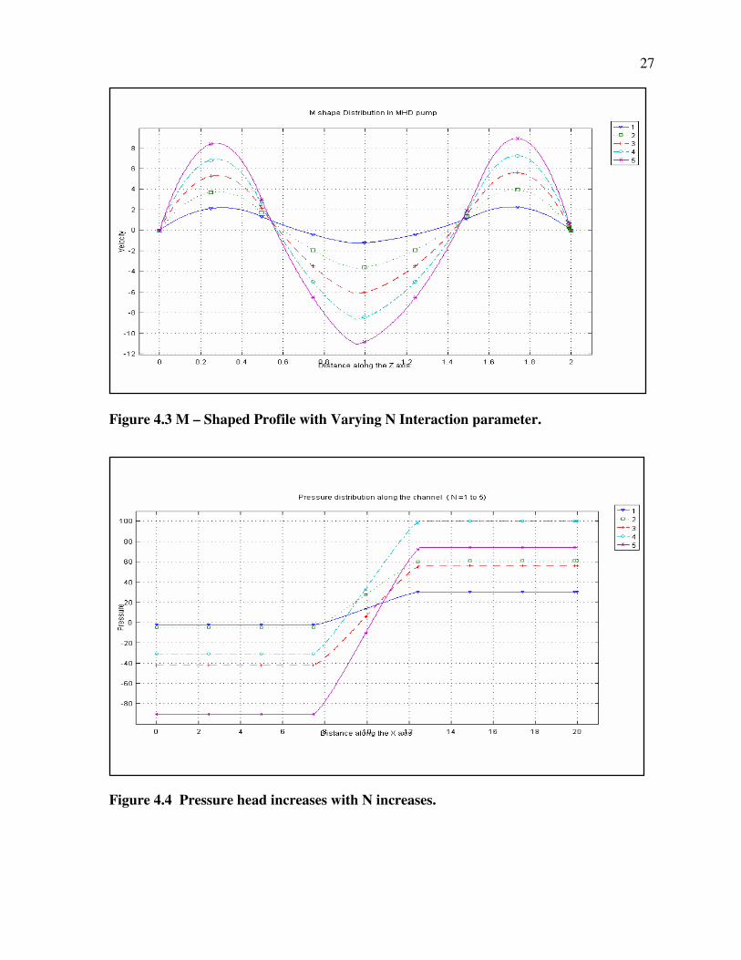
Figure 4.4 Pressure head increases with N increases..............................................................27
Figure 4.5 Pinch effect for Le = 5............................................................................................28
Figure 4.6 Pinch effect increases with Length of the electrode decreases. Le = 1. .................29
Figure 4.7 Dependence of flow velocity on depth in rectangular channels of different
widths...........................................................................................................................31
Figure 4.8 Dimensions of MHD channel considered for evaluation of electroosmotic
velocities. .....................................................................................................................33
Figure 4.9 The effect of depth reduction on the electroosmotic velocity (VEO) in
rectangular MHD micropump......................................................................................33
Figure 4.10 Geometry of nozzle/diffuser section. ...................................................................35

x
Figure 4.11 Velocity distribution along the channel length of a nozzle-diffuser flow
cell................................................................................................................................35
Figure 4.12 Velocity distributions in a nozzle-diffuser MHD flow-cell (depth and
width directions).. ........................................................................................................36
Figure 4.13 Dependence of velocity on depth in nozzle-diffuser shaped channels of
different widths. ...........................................................................................................36
Figure 4.14 (U x B) term contribution to current density. .......................................................37
Figure 4.15 Current density (J) distribution along the x-axis (y = b/2, z=d/2). .......................37
Figure 4.16 Dependence of velocity on diffuser angle in nozzle-diffuser shaped
channels........................................................................................................................39
Figure 4.17 Current density (J/Area) distribution in a cross-section of a trapezoidal
channel at different depths. d is the depth of the channel. ...........................................40
Figure 4.18 Streamlines of magnetic flux density in a trapezoidal shaped MHD
pump.. ..........................................................................................................................40
Figure 4.19 Lorentz Force (FL) distribution in a cross-section of a trapezoidal channel
at different depths.. ......................................................................................................41
Figure 5.1 The effect of depth reduction on the electroosmotic velocity (VEO) in a
trapezoidal MHD micropump. .....................................................................................45
Figure 5.2. The effect of depth reduction on Joule heating in rectangular MHD
micropump... ................................................................................................................47
Figure 5.3 The variation of conductivity of electrolyte along the centerline of MHD
pump of rectangular cross-section due to Joule heating. .............................................48
Figure 5.4 The effect of Joule heating on the Lorentz’s force in rectangular MHD
micropump. ..................................................................................................................48

xi
ACKNOWLEDGEMENTS
Special thanks to Dr Samuel Kinde Kassegne for his perception, supervision and
support during the development of thesis and throughout my education at San Diego State
University.
Thanks to Mechanical Engineering Department at SDSU for providing me valuable
education. Last, but not least, thanks to all my friend and colleagues from the Micro Electro
Mechanical System Research Laboratory.

1
CHAPTER 1
INTRODUCTION
MEMS (Micro ElectroMechanical Systems) are in the process of revolution industries
varying from consumer electronics to life sciences are wondered to be successful. Their
falling prices enabled by batch processing configured with the integration of a whole system
in an extremely small foot print (often in µm2 and mm
2) have contributed to their success. In
the life science, Labs-On-a-Chip (LOC) is considered to be one of the most useful MEMS
applications. In these LOC systems, one of the main requirements is to precisely and
effectively control small volume of buffer.
Micropumps are mainly classified into two categories. (i) Mechanical micropumps
and (ii) Non-mechanical micropumps [1]. In mechanical micropumps, a membrane is used
to generate pumping action. This excitation of membrane can be produce by electrostatical
[2], thermo pneumatical [3], pneumatical [4], piezoelectrical [5], [6] or electromagnetical [7]
mechanisms. Major advantage of mechanical pumping mechanism is less dependability on
buffer or fluid solution. But it requires high voltage (100V-200V) to actuate the membrane
and it has intermittent force rather than continues fluid force.
On the other hand, non-mechanical micro pumps have no moving parts. So they do
not have any wear or fatigue problems. Non-mechanical micropumps are actuated by various
mechanisms depending upon the proposed applications. Examples include electro-
hydrodynamic pumps (EHD) [8] which pump dielectric fluid or buffer, electrokinetic pumps

2
[9-10], which is further, classified into electroosmosis and electrophoretic pumping
mechanism and magnetokinetic pumps (MHD) [11].
Bubble micropumps [12] and electrochemical micropumps also fall in the category of
non-mechanical type of micropumps. To pump biological fluid only electrokinetic and
magnetokinetic pumps are suitable. It is mainly applicable to µTAS (Micro Total Analysis
Systems) where separation is needed. For other biological systems syringe pumps are
utilized.
Among all of these pumping mechanisms, this thesis focused on a non-mechanical
type MHD micropump that works on the principle of Lorentz Force. Magnetohydrodynamic
micropumps have recently attracted a wide attention in micro fluidic research, particularly in
LOC (Lab-On-a-Chip) devices and µTAS. MHD works on the principle of Lorentz Force,
which is generated by applying an electric current to the conductive liquid across the channel
in the presence of a perpendicular magnetic field. This is illustrated in Figure 1.1.
F = J x B x VD
where,
F = Lorentz Force,
J = Current density = Current / Area (Amp/m2)
B = Magnetic Field (Tesla)
VD = Device volume (m3)
AC magnetohydrodynamic pumps produce continues flow and are suitable for
biological liquid. These pumps can be used as a multiple, independently controlled pumps
system on integrated chips [13].
This thesis manuscript reports analytical investigation of the physics of this devices
and development of the numerical framework of the 3-D MHD equations governed by the

3
Figure 1.1 Typical configuration of MHD micro pumps with a rectangular cross-
section.
multi physics of MHD micropump. There has been always a research interest on the
theoretical and experimental comparison of the MHD flow in micro channels.
Thesis is configured as follows: Chapter 1 covers introduction to MEMS and Labs-
On-a-Chip (LOC) systems. Chapter 2 covers literature survey where as Chapter 3 develops
the 3-D MHD equations. Numerical results are discussed in Chapter 4. And finally Chapter 5
gives conclusions based on the consequential numerical outcome.
There are various physics acting on the fluid while applying a current and magnetic
field on the side of the rectangular or trapezoidal channel, such as non-uniform electric field,
electroosmosis and joule heating. The investigation of these physics in the context of
developing complete 3-D MHD equations for micropumps is therefore, the focus of this
research.

4
Therefore, it is clear that the need for defining rational analytical and numerical
framework for the solution of the most general 3-D MHD equations tailored for the physics
and scale of micropumps remains un-met. Work formulates a general numerical framework
for the 3-D MHD equations for micropumps. With the developed framework, we solve the
MHD equations for a variety of geometrical cross-sections of micropumps. The numerical
framework makes no simplifying assumptions on the geometry of cross-section and is –
therefore – applicable to any potential MHD micropump configuration. Further, we also
investigate the effects of double layers (and hence electroosmosis) on the Lorentz force
driven fluid flow. We also model Joule heating in the flow cell and investigate the
distribution of temperature and effects on the main fluid flow.
5
CHAPTER 2
LITERATURE SURVEY
2.1 MHD PHYSICS
W. Ritchie was the first who discovered the MHD phenomenon in 1832 [14]. He
described the basic operating principle of such micropumps where, an electrical current and a
perpendicular magnetic field pass through an electrolytic solution, thereby producing a
Lorentz force along the length of the channel of the micropump. MHD was historically
mainly used in the propulsion system, electromagnetic breaks and nuclear fusion. [50-52]
2.2 MACRO AND MICRO MHD PHENOMENON
For macro MHD applications such as marine vehicle propulsion, electromagnetic
breaks (Reversed Lorentz Force), nuclear reactor cooling and metal drawing, etc., a wealth of
information on rational fluid flow analysis based on the solution of the so-called Non-
Dimensional Analysis (NDA) MHD equations exists [15-17]. In general, these macro
specific MHD equations were solved for a regime of moderate to high Hartmann number
(Ha, ratio of Lorentz force to viscous forces) and interaction parameters (N, ratio of Lorentz
force to inertia forces).
Hunt and Stewartson [18] have performed one of the earliest asymptotic analysis of
MFD (magneto fluid dynamics) for electromagnetic pumps. For limiting case of Hartmann
number, which is a ratio of Lorentz force to Viscous force (M>>1), numerical studies were
performed for various combination of electrical conductivities such as insulating/conductive
6
side walls with parallel and perpendicular to the uniform applied magnetic field. Here flow
was assumed to be fully developed.
Huges and McNab [19] derived an overall pump efficiency while extending the
analysis to include magnetic fringe effect. A quasi one-dimensional lumped circuit model
was used to obtain electrical characteristics of the walls and fluid in the pump region. They
have also shown parametric plots of pump efficiency with function of basic design variable.
Hughes [20], Turner [21], Walker [22] and Holroyd [23] also made significant
contribution. Branover et al. [24, 25] reported experimental effort on high Hartman number
and Interaction parameter flows. All these theoretical analysis have used assumptions which
simplify the full governing equations for limiting range of operations. Singh and Lal [26]
employed numerical analysis same as Winowich and Hughes’s Finite Element Analysis of 2–
D MHD flow [27]. Gel et al. used a stream function-vorticity Finite Difference Formulation
to analyze MHD channel flows [27].
Yagawa and Masuda [28] used an incremental Finite Element Techniques to study
MHD flows for high magnetic Re numbers where the induced magnetic field can not be
neglected. They have also analyzed a lithium blanket at high interaction parameter where
they neglected convection and viscous terms in the Navier-Stokes equation.
Later Winowich and Hughes [29] analyzed a DC electromagnetic pump with
insulating (nonconductive) side walls at low interaction parameter N using the Finite Element
Method. This time they also solved the complete Navier-Stokes with a nonuniform applied
magnetic field.
Ramos and Winowich [30] used time dependent primitive variable Finite Difference
method to solve electromagnetic pump. They showed that in order to get fully developed

7
MHD flow, upstream and downstream boundaries should be much far away from electrodes
in case of nonconductive walls. They also reported that locations of these boundaries are
function of Reynolds number and Interaction parameter and the resulting velocity M-shaped
profile in the vicinity of magnetic field.
Winowich et al. [29] calculated MHD channel flow as a function of electrode length
and wall conductivity and also showed that channel wall electric potential increases as wall
conductivity increases. Ramos and Winowich [30] reported that the difference between Finite
Difference and Finite Element method were due to different meshes employed in analysis.
Winowich and Hughes’s [31] unrealistic NDA approach resulted, the effect of the
Reynolds number, interaction parameter, electrode Length and wall conductivity on the
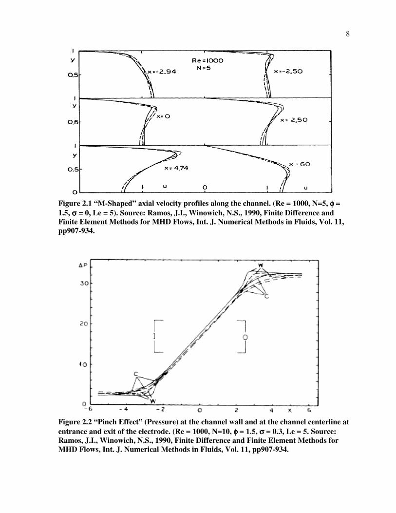
MHD field. Study of such a comparison also indicated that “M-Shape” velocity profile
(Figure 2.1) and “Pinch Effect” (Figure 2.2) is more pronounce in primitive-variable finite
difference formulation than the stream function vorticity and finite element method.
Magnetohydrodynamic micropumps have been investigated by Lemoff and Lee [13]
(Figure 4), Jang and Lee [32], Huang et al. [34], Heng et al. [35], [36], Bao and Harrison
[37], P. J. Wang [38], Homsy et al. [39], and other researchers have attracted significant
attention in the microfluidics community. The main reasons for the significant interest in
MHD micropumps are the absence of moving parts, simple fabrication processes, lower
actuation voltages, reduced risk of clogging and damage to molecular materials, reduced risk
of mechanical fatigue and a continuous fluid flow (Figure 2.3).
However, reports on rigorous analytical and numerical modeling of the MHD
equations for microfluidics applications – pertinent to their unique physics and very low
Hartmann number regime – are scarce and have just barely begun to appear in the literature.
8
Figure 2.1 “M-Shaped” axial velocity profiles along the channel. (Re = 1000, N=5, φφφφ =
1.5, σσσσ = 0, Le = 5). Source: Ramos, J.I., Winowich, N.S., 1990, Finite Difference and
Finite Element Methods for MHD Flows, Int. J. Numerical Methods in Fluids, Vol. 11,
pp907-934.
Figure 2.2 “Pinch Effect” (Pressure) at the channel wall and at the channel centerline at
entrance and exit of the electrode. (Re = 1000, N=10, φφφφ = 1.5, σσσσ = 0.3, Le = 5. Source:
Ramos, J.I., Winowich, N.S., 1990, Finite Difference and Finite Element Methods for
MHD Flows, Int. J. Numerical Methods in Fluids, Vol. 11, pp907-934.
9
Figure 2.3 MHD Micropump fabricated by A. b. Lee and Lemoff & V. Patel, S.
Kassegne & E. Bao (Publication under progress).
Almost all of these studies had assumed the flow inside such flow cells to be a one-
dimensional fully developed laminar flow where Poiseuille type conditions were used to
solve for velocity distributions [38]. This assumption of Poiseuille type conditions which
neglects the side-wall frictional effects is, however, too simplistic to capture the complex
three-dimensional behavior of the fluid flow fields under the most general geometry and
magnetic and electric field distribution conditions. As an improvement, Wang et al. [38] used
the decoupled and simplified 2-dimensional version of the MHD equations where the Lorentz

10
forces were substituted as a pressure in the momentum equations. The ensuing simplified
equations were then solved using the finite difference method. Their formulation assumed an
axially invariant velocity distribution; thereby limiting the scope of their numerical solution
to channels of uniform cross-section and uniform Lorentz force with no provision for
arbitrary channel geometries, and magnetic and electric field distributions. At this point,
however, the 3-D version of the MHD equations has not been solved yet for MHD
micropumps used in microfluidics applications. Furthermore, neither experimental nor
theoretical investigations of the effects of electric double layer on the dielectric surfaces of
MHD micropumps have been reported in the literature yet. With regard to Joule heating,
Homsy et al. [39] have discussed experimental observations where they noted that, beyond a
certain current threshold, Joule heating affected velocity measurements; but rational
analytical solutions still remain un-attempted. To avoid disruption of flow due to bubble
creation Homsey et al. [39] have designed MHD main channel with 2 side channel.
Electrodes are physically separated from main channel in which flow is generated. So bubble
formed in side channel can not obstruct the flow of main channel (Figure 2.4).
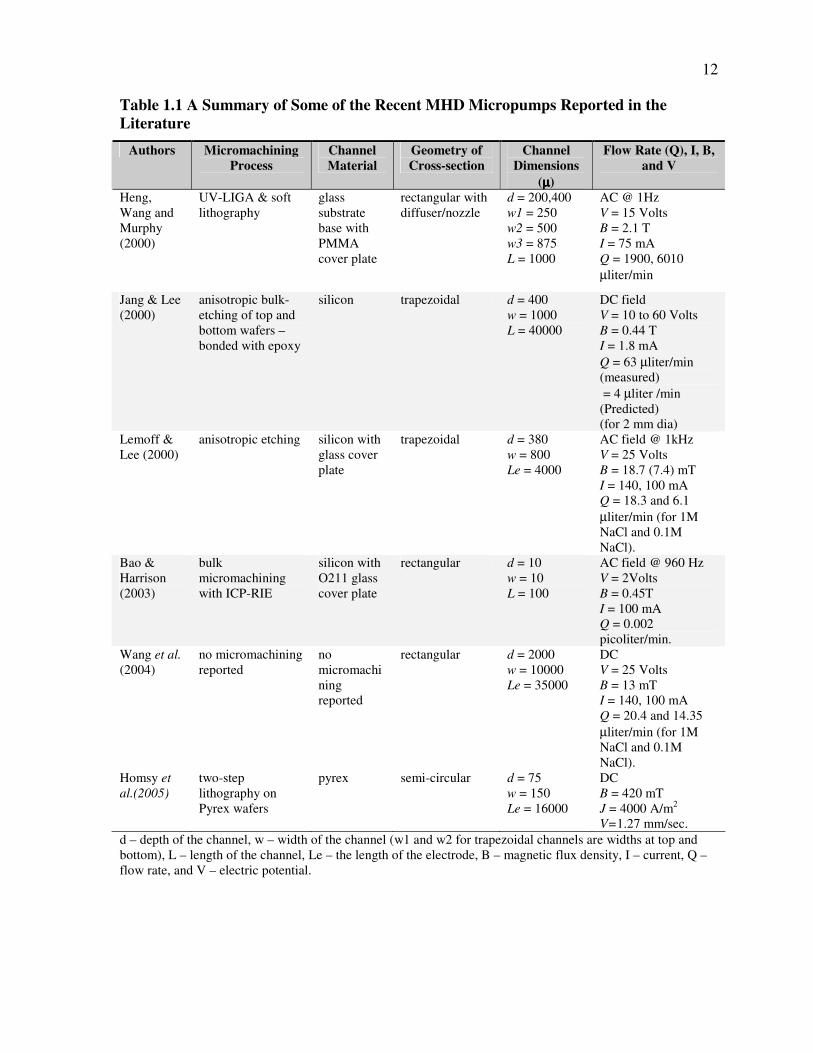
To provide a perspective to the range of MHD micropumps considered in this and
other studies, Table 1.1 summarizes some of the typical micropump configurations reported
by previous researchers. The table also summarizes the micromachining processes, materials
and the geometrical dimensions and reported flow rates. The sizes of the micropumps vary
from 2 mm deep [38] to 10 µm by 10 µm [37]. Current and magnetic flux densities vary from
a maximum of 140mA [13] and 2.2 Tesla (T) [34] to 1.8mA [32] and 420 mT [39]. The flow
rates vary from 6010 µliter/min for the nozzle/diffuser micropump of [34] Heng, Wang and
Murphy to 720 picoliter/min of [37] Bao & Harrison. Both AC and DC sources have been

11
Figure 2.4 MHD Micropump fabricated by Homsey et al. Source: Homsy, A, Koster, S,
Eijkel, JCT, Berg, A, Lucklum, F, Verpoorte, E, and de Rooij, NF, 2005, A high current
density DC magnetohydrodynamic (MHD) micropump, Lab Chip, 5(4), pp466-471.
used. With regard to micromachining processes, bulk micromachining of silicon using LIGA,
ICP-RIE (inductively coupled plasma reactive ion etching), and anisotropic wet etching
together with soft lithography have been used. Table 1.1 also demonstrates that MHD
micropumps are being increasingly miniaturized with the smallest such device reported
currently being at a range of 10 µm. It should be noted, however, that the numerical
framework developed in this study is applicable to fluid flow in MHD micropumps where the
channel dimensions are 100 um and higher where Navier-Stokes Equations hold true.
12
Table 1.1 A Summary of Some of the Recent MHD Micropumps Reported in the
Literature
Authors Micromachining
Process
Channel
Material
Geometry of
Cross-section
Channel
Dimensions
(µµµµ)
Flow Rate (Q), I, B,
and V
Heng,
Wang and
Murphy
(2000)
UV-LIGA & soft
lithography
glass
substrate
base with
PMMA
cover plate
rectangular with
diffuser/nozzle
d = 200,400
w1 = 250
w2 = 500
w3 = 875
L = 1000
AC @ 1Hz
V = 15 Volts
B = 2.1 T
I = 75 mA
Q = 1900, 6010
µliter/min
Jang & Lee
(2000)
anisotropic bulk-
etching of top and
bottom wafers –
bonded with epoxy
silicon trapezoidal d = 400
w = 1000
L = 40000
DC field
V = 10 to 60 Volts
B = 0.44 T
I = 1.8 mA
Q = 63 µliter/min
(measured)
= 4 µliter /min
(Predicted)
(for 2 mm dia)
Lemoff &
Lee (2000)
anisotropic etching silicon with
glass cover
plate
trapezoidal d = 380
w = 800
Le = 4000
AC field @ 1kHz
V = 25 Volts
B = 18.7 (7.4) mT
I = 140, 100 mA
Q = 18.3 and 6.1
µliter/min (for 1M
NaCl and 0.1M
NaCl).
Bao &
Harrison
(2003)
bulk
micromachining
with ICP-RIE
silicon with
O211 glass
cover plate
rectangular d = 10
w = 10
L = 100
AC field @ 960 Hz
V = 2Volts
B = 0.45T
I = 100 mA
Q = 0.002
picoliter/min.
Wang et al.
(2004)
no micromachining
reported
no
micromachi
ning
reported
rectangular d = 2000
w = 10000
Le = 35000
DC
V = 25 Volts
B = 13 mT
I = 140, 100 mA
Q = 20.4 and 14.35
µliter/min (for 1M
NaCl and 0.1M
NaCl).
Homsy et
al.(2005)
two-step
lithography on
Pyrex wafers
pyrex semi-circular d = 75
w = 150
Le = 16000
DC
B = 420 mT
J = 4000 A/m2
V=1.27 mm/sec.
d – depth of the channel, w – width of the channel (w1 and w2 for trapezoidal channels are widths at top and
bottom), L – length of the channel, Le – the length of the electrode, B – magnetic flux density, I – current, Q –
flow rate, and V – electric potential.
13
CHAPTER 3
MULTI-PHYSICS OF MHD PUMP
3.1 DEVELOPMENT OF 3-D EQUATION
The physics of magnetohydrodynamics for most macro level applications is now
relatively well developed [15-18, 26]. In the most general form, the physics of
electromagnetism and incompressible fluid dynamics are the predominant physics of interest
for macro level MHD applications. For MHD micro-pumps which are typically of several
hundred of microns dimensions and fabricated using MEMS processes such as silicon/glass
bulk micro-machining and soft lithography (Figure 1.1 and Table 1.1). However, their unique
scale and material properties require that additional physics be accounted for to accurately
capture their behavioral response to external effects.
One such physics is electroosmosis, which is the bulk movement of an aqueous solution
under an external electric field [40]. In MHD micropumps - much like most microfluidic
devices, electroosmosis is caused by the existence of a zeta potential at the interface between
the silicon or glass linings and the electrolyte. This zeta potential is formed due to the
dissociation of ions or ionic groups and extends over a thin layer at the interface between the
glass/silicon/metal linings of the micropump and the electrolyte. This thin layer is called an
electrical double layer and has a typical thickness of less than 10 nm (Debye’s length). Another
physics that is considered in this study is the physics of Joule heating. Typically, in a
conductive media such as an electrolyte, an electric field causes heating and change in

14
temperature distribution. This change in temperature will in turn cause a decrease in viscosity
and increase in conductivity of the electrolyte. A 2% increase in conductivity per degree rise in
electrolyte temperature is considered a typical value [41]. Further, thermal heating of an
electrolyte also causes electrothermal forces that contribute to fluid velocity increases [42].
For deriving a more-general MHD set of equations applicable for MHD micropumps
and a numerical framework for their solution, the general MHD equations such as those
reported by [31] serve as a starting point. Four distinct sets of equation systems are considered
here; electromagnetic system, fluid dynamic system, electrokinetic system and a thermal
system. The electromagnetic system consists of the Gauss Law and Magnetic Induction
Equation along with Poisson’s Equation and Ohm’s Law. These equations define the
distribution of the magnetic flux density, the electric field and the current density
(Eqs. 1.a – 1.e) respectively. In its general form, the Magnetic Induction Equation suggests that
the motion of a conducting liquid (electrolyte) in an applied magnetic field induces a magnetic
field in the medium through a ∇∇∇∇ x (U x B) term. The total magnetic field is, therefore, the sum
of the applied and induced magnetic fields. The relative strength of the induced field is often
characterized by a dimensionless number; the magnetic Reynolds number, Rem= σµmUL,
where σ is the electrical conductivity, µm – the magnetic permeability, U – the velocity and
L – the length of the channel. For typical electrolytes used in biological microfluidics
applications, Rem is small and, therefore, the induced magnetic field is often neglected as is the
case in this work.
The fluid dynamic system consists of the continuity equation and Navier-Stokes
equation that define the physics of bulk fluid flow (Eqs. 3.a and 3.b). Helmholtz-
Smoluchowski equation for electroosmotic flows (Eq. 4) forms the electrokinetic system
15
whereas the energy balance equation (Eq. 5.a) and the time averaged electrothermal force
equation, given by Eq. 5.b [42], form the thermal system. In Eq. 5.b, the first part is the
Coulombic force dominant at low frequencies whereas the second part is the dielectric force
dominant at higher frequencies (and also DC). Combined together, the full three-dimensional
MHD equations that govern the physics of MHD micropumps including the reverse Lorentz
force, the non-zero zeta-potential on flow channel walls and Joule heating are given by
Equations (1-5). These equations are coupled. The boundary conditions for each of the
equation systems are given in Table 2.1.
To solve these equations in an iterative manner, the following assumptions are made.
The flow is assumed to be fully developed and laminar (low Reynold’s number). The fluid has
low conductivity; as the fluids of interest are typical electrolytes used in biological
applications. Consequently, the Hartmann number, Ha (σB2L
2/µ)
0.5 and the interaction
parameter, N (σB2L/ρU) are both small (where B is the magnetic flux density, σ - electric
conductivity of fluid, µ - viscosity, ρ – density of fluid, L – length of channel, and U - velocity
vector). The current induction from a moving fluid under a magnetic field is assumed to be
negligible; thereby decoupling the magnetic induction and magnetic line closure relationships
[15], [43]. Further, the Debye length (often in the range of 10 nm or so) is assumed to be very
small compared to the channel width. This enables the use of the Helmholtz-Smoluchowski
equation to represent electroosmosis. Under these assumptions, then, the full 3-D MHD
equations for an isotropic incompressible Newtonian fluid used in a micro-scale are formally
written as follows:

16
Table 2.1 Boundary Conditions for Generalized 3D Rectangular MHD Equations for
MHD Micro Fluidics Pumps
Equation Type Boundary Condition
Electromagnetics B(x,y,o) = known (+) (x < Le)
B(x,y,d) = known (-) (x < Le)
Electrodes
Φ(x,0,z) = V (x < Le)
Φ (x,b,z) = - V (x < Le)
Insulations
Magnetically insulated elsewhere
Electrically insulated elsewhere
Fluid Dynamics U(x,0,z) = 0 (no-slip), U(x,y,0) = 0 (no-slip)
U(x,b,z) = 0 (no-slip), U(x,y,d) = 0 (no-slip)
Inlet
U(0,y,z) = 0
Outlet
P(L,y,z) = 0
body force = FL (Lorentz Force)
Electrokinetics U(x,y,0) = UEO (slip)
U(x,y,d) = UEO(slip)
Thermal System T(x,y,0) = Room Temperature 25oC (isothermal with outside) at bottom magnet
T(x,0,z) = Room Temperature 25oC (isothermal with outside) at electrode
T(x,b,z) = Room Temperature 25oC (isothermal with outside) at electrode
T(x,y,d) = k∇T (free convective flux) at top magnet
Q(0,y,z) = sero flux where Q is the heat flux
Q(l,y,z) = sero flux
(i) Electromagnetic system:
The magnetic field components are given as:
0. =∇ B (Gauss Law / Magnetic line closure) (1.a)
Bt
B 21∇=
∂
∂
σµ (Magnetic Induction) (1.b)
The electrical field components are:
∇2Φ = ∇.(U x B) (Poisson’s Equation) (1.c)
Φ−∇=E (1.d)
J = σ (E + U x B) (Ohm’s Law) (1.e)
The Lorentz force is then given as,
17
FL = (J x B) Le (2)
(ii) Fluid dynamics system:
0. =∇ U (Continuity Equation) (3.a)
ETL FFUpUUDt
DU++∇+−∇=∇+ 2).( µρ (Navier - Stokes Equation) (3.b)
(iii) Electrokinetic system:
Φ∇−= EOEOU µ , where µζεµ /=EO (Helmholtz-Smoluchowski Equation) (4)
(iv) Thermal system:
σρ
22).(
JTkTU
Dt
DTC p +∇=∇+ (5.a)
∇+
+
∇
−∇
−= εωτ
ε
ε
ε
σ
σ 2
2 2
1
)(12
1E
EEFET (5.b)
where, p – fluid pressure, J - current density vector, T - temperature, t – time, Φ – electric
potential, E – electric field, UEO – electroosmotic velocity, µEO – electroosmotic mobility,
Cp – specific heat, k – thermal conductivity, ζ – zeta potential, ε – dielectric permittivity,
τ =ε/σ - the charge relaxation time of fluid, ω – the frequency of the AC electric field, Le – the
electrode length, FET – Electrothermal force, and FL – Lorentz force.
For steady-state conditions, the left hand sides of Eqs 3.b and 5.a reduce to zero. The
3-D MHD equations given here are conveniently solved using any finite element discretization
approach. COMSOL multiphysics [44] FEA modeling software is used for the solution of these
equations. The mesh sizes differ depending on the geometry under consideration; however
quadratic elements are used with enough refinement for convergence. Due to the coupling
between these sets of equations, an iterative solution approach is used. First, the

18
electromagnetic components have been given by the Gauss Law and the Magnetic Induction
Law (Eqs. 1.a and 1.b) are solved to determine the magnetic flux density (B). It is instructive to
recognize that these equations form part of the Maxwell equations [43]. The electric potential
(Φ), the electric field (E) and current densities (J) are then determined by solving the Poisson
Equation and Ohm’s Law (Eq. 1.c, 1.d and 1.e). In the initial run, the component of the current
density that comes from the cross product of the velocity and the magnetic field (i.e., U x B) is
zero as the fluid velocity is not yet determined. The Lorentz force is then evaluated as a vector
cross product of the current vector and the magnetic flux density vector (Eq. 2). The Lorentz
force is then applied as a body force in the Navier-Stokes equation. This is followed by the
solution of the 3-dimensional continuity and Navier-Stokes equations (Eqs. 3.a and 3.b). Once
the vectorial flow velocity distribution (U) is determined, the electrical field components (i.e.,
Φ, E and J) are re-evaluated by adding the current component from the vector cross product of
the velocity and the magnetic field (i.e., U x B) to Eqs. 1.c – 1.e. Subsequently, for a given
iteration, the thermal system is solved using Eq. 5.a; the quantity of interest being the
temperature profile (T). The Lorentz’s force FL and the electrothermal force FET (Eqn 5.b) are
then updated and the Navier-Stokes Equations are re-solved. This iterative process is repeated
until the velocity (U), the temperature (T), and the electric field (E) converge to within a pre-
set cut-off limit. Here a cut-off limit of |Un+1 – Un| / |Un| ≤ 1.0*10-6
, |En+1 – En| / |En| ≤
1.0*10-6
, and |Tn+1 – Tn| / |Tn| ≤ 1.0*10-6
are used where ‘n’ and ‘n+1’ represent the iteration
numbers. The electroosmotic velocity component (UEO) is determined using the Helmholtz-
Smoluchowski equation given in Eq. 4.

19
3.2 FORMULATION OF EQUATIONS FOR
NON-DIMENSIONAL ANALYSIS
A distinct approach is considered to solve MHD equations, called Non-Dimensional
Analysis. Non-Dimensional analysis involves the determination of hydrodynamic flow in the
channel as a function of the Reynolds number (Re), interaction parameter (N), electrode
length (Le). This study considers MHD flows where magnetic field is perpendicular to the
flow direction. This non-uniform applied magnetic field produces M shaped velocity profiles
in the MHD pump region. Results obtained in this thesis are in qualitative agreement with the
2-D asymptotic analysis of reference [16, 17, 26, 27, 29, 30, 31].
3.2.1 Problem Description
The pump includes of a channel, two electrodes and two magnetic pole pieces
(Figure 3.1).
Hydrodynamic and magnetic field are 3-Dimensional. The flow in this problem is
assumed as steady, incompressible, laminar, isothermal, Newtonian and electrically
conducting. Electrodes are perfect conductors.
All the constitutive equations are based on the dimensions that are described as below:
Channel width: 2b, Electrode length = 2 Xe (-Xe to + Xe). Where Xe= Unit electrode length
The 3-D non-dimensional with formulations is given as below:
(i) Non dimensional parameters.
b
xx =*
b
yy =*
um
uu =*
vm
vv =*
( )2*
um
pp
ρ= (6 a, b, c, d, e)
(ii) 3-D Hydrodynamic NDA equations (Navier-Stokes).

20
Figure 3.1 MHD Pump with unit dimension consideration. Source: W. Zhang, C.H.
Ahn, in: A Bi-Directional Magnetic Micropump on a Silicon Wafer,Solid-State Sensor
and Actuator Workshop, Hilton Head, SC, 1996, p. 94.
**
*
*
*
*
*
Re
1
*
*
*
**
*
**
*
**
2
2
2
2
2
2
xFz
u
y
u
x
u
x
p
z
uw
y
uv
x
uu +
∂
∂+
∂
∂+
∂
∂+
∂
∂−=
∂
∂+
∂
∂+
∂
∂ (7 a)
**
*
*
*
*
*
Re
1
*
*
*
**
*
**
*
**
2
2
2
2
2
2
yFz
v
y
v
x
v
y
p
z
vw
y
vv
x
vu +
∂
∂+
∂
∂+
∂
∂+
∂
∂−=
∂
∂+
∂
∂+
∂
∂ (7 b)
**
*
*
*
*
*
Re
1
*
*
*
**
*
**
*
**
2
2
2
2
2
2
zFz
w
y
w
x
w
z
p
z
ww
y
wv
x
wu +
∂
∂+
∂
∂+
∂
∂+
∂
∂−=
∂
∂+
∂
∂+
∂
∂ (7 c)
Where um = Mass Avg. velocity ( )µ
ρ muRe
b= . (7 d)
And ( )2
*mu
FxbFx
ρ=
( )2*
mu
FybFy
ρ= (7 e, f)

21
(iii) Electric field
φgradE −= So *** φgradE −= (8 a, b)
(iv) Magnetic field (B is assumed to act in the Z direction only)
( )BzB ,0,0= So Bo
BzBz == 1* (9 a, b)
(v) Current Density (J is related to E)
( )BvEJ ×+= σ So ( )**** BvERmJ ×+= where
µbB
JJ
1* = (10 a, b)
(vi) Body Force F = (Fx, Fy, Fz) which is the Lorentz force given by,
( )[ ] BBvEBJF ××+=×= σ (11 a)
( ) ( )[ ] ******** BBvgradNBJAF ××+−=×= φ (11 b)
where,
Alfven Number( )2
2
um
BoA
µρ= (11 c)
and Interaction parameter ( )( )um
bBoN
ρ
σ 2
= (11 d)
So Body force in term of non dimension parameter would be,
( ) ( ) ***
*** 2 uBN
yBNF zzx −
∂
∂−=
φ (11 e)
( ) ( ) ***
*** 2
vBNz
BNF zzy −∂
∂−=
φ (11 f)
( ) ( ) ***
*** 2
wBNx
BNF zzz −∂
∂−=
φ (11 g)
22
Similar to equations 1.a – 5.b, their NDA equations are numbered. We use COMSOL
multiphysics [44] in a NDA format iteratively to solve these equations. The 3-D MHD
equations given here are conveniently solved using any finite element discretization approach.
The mesh sizes differ depending on the geometry under consideration; however quadratic
elements are used with enough refinement for convergence. Due to the coupling between these
sets of equations, an iterative solution approach is used. First, the electromagnetic components
have been given by the Gauss Law and the Magnetic Induction Law (Eqs. 1.a and 1.b) are
solved to determine the magnetic flux density (B). It is instructive to recognize that these
equations form part of the Maxwell equations [43]. The electric potential (Φ), the electric field
(E) and current densities (J) are then determined by solving the Poisson Equation and Ohm’s
Law (Eq. 1.c, 1.d and 1.e). In the initial run, the component of the current density that comes
from the cross product of the velocity and the magnetic field (i.e., U x B) is zero as the fluid
velocity is not yet determined. The Lorentz force is then evaluated as a vector cross product of
the current vector and the magnetic flux density vector (Eq. 2). The Lorentz force is then
applied as a body force in the Navier-Stokes equation. This is followed by the solution of the
3-Dimensional continuity and Navier-Stokes equations (Eqs. 3.a and 3.b). Once the vectorial
flow velocity distribution (U) is determined, the electrical field components (i.e., Φ, E and J)
are re-evaluated by adding the current component from the vector cross product of the velocity
and the magnetic field (i.e., U x B) to Eqs. 1.c – 1.e. The Lorentz’s force or Body force FL is
calculated by NDA approach defined in Eqs. 6.a – 11.g. Similar to this, velocity at inlet and
outlet is assumed as well known parabolic profile equation (Table 2.2 and 2.3).
23
Table 2.2. Subdomain Conditions for Generalized 3D Non-Dimensional Rectangular
MHD Equations for MHD Micro Fluidics Pumps
Equation Type Subdomain Settings
Electromagnetics Electrical
σ = N (Interaction parameter)
Magnetic
Permittivity = 1 (All demain)
Fluid Dynamics Density ρ = 1,
Dynamic viscosity µ = 1/ Re
Force Fx* = ( N * I0* Bz* - N Bz*² u* )
Where I0* = Current in Amp
Table 2.3. Boundary Conditions for Generalized 3D Non-Dimensional Rectangular
MHD Equations for MHD Macro Fluidics Pumps
Equation Type Boundary Condition
Electromagnetics Magnetic (Magnetic Field density)
B(x,y,o) = 1(+) (x < Le)
B(x,y,d) = 1 (-) (x < Le)
Electrodes (Current Density)
J(x,0,z) = I/Area (x < Le)
J(x,b,z) = I/Area (x < Le)
Insulations
Magnetically insulated elsewhere
Electrically insulated elsewhere
Fluid Dynamics U(x,0,z) = 0 (no-slip), U(x,y,0) = 0 (no-slip)
U(x,b,z) = 0 (no-slip), U(x,y,d) = 0 (no-slip)
Inlet
U(u,y,z) = 1.5*(1– (y^2))*(1-(z^2))
Outlet
U(u,y,z) =1.5*(1–(y^2))*(1-(z^2))
Body force = FL (Lorentz Force)

24
CHAPTER 4
PRESENTATION OF RESULTS AND DISCUSSION
4.1 VALIDATION OF RESULTS BY NON-DIMENSIONAL
ANALYSIS
The purpose of the NDA analysis is to get validity for the FEA code used in
micropump simulation. This chapter is the extension of 2-D to 3-Dimensional of Winowich et
al. [31] (1990)’s. As derived in chapter 3 non-dimensional analysis involves simulation based
on the dimensionless numbers. The sub-domain and boundary setting are applied with
generally unit number or made to equal to unity for NDA analysis.
As shown in Figure 2.2, unit geometry has been considered to solve the problem
analytically. Once again the pump includes of a channel, two electrodes and two magnetic
pole pieces (Figure 2.2). The flow in this problem is assumed to be steady, incompressible,
laminar, isothermal, Newtonian and electrically conducting. Electrodes are perfect
conductors. A Finite Element Method is used to solve velocity and pressure distribution
along the channel line. Different approaches are considered here to solve flow distribution.
4.1.1 Reynolds Number and Effects
Figure 4.1 and 4.2 show the velocity and pressure distributions along the channel line.
Comparison shows that as Reynolds number increases from Re = 1- 500 for Le = 5, and N =
5. The back flow and eventually M-shaped velocity profile becomes more prominent in
MHD pumping area. Pressure head along the line remains same with varying Re.

25
Figure 4.1 M-Shaped velocity profile along the channel line as Reynolds number
increases.
Figure 4.2 Pressure distribution along the MHD region with varying Re.

26
4.1.2 Interaction Parameter Effects
Figure 4.3 and 4.4 show the effect of interaction parameter velocity and pressure
distributions. Back flow and therefore “M – Shaped” velocity profile becomes more
pronounce as N increases from 1 to 5. Interaction parameter also has an effect on pressure
head along the channel. Figure 4.5 shows that pressure increases in the MHD region as N
increases.
4.1.3 Electrode Length Effect (Pinch Effect)
Finite Element Model shows a pressure rise at the wall and at the center of the
channel due to presence of the electromagnetic body forces. It is assumed that this wall
pressure is caused by the Lorentz force and that exhibits the so called “Pinch Effect” at the
electrode entrance and exit (Figure 4.5).
This pinch effect becomes more pronounce as Length of the channel decreases.
Figure 4.6 shows that as electrode length and so MHD pumping region decreases, “Pinch
Effect” becomes more distinguished.
4.2 MHD MICROPUMP WITH DIFFERENT CHANNEL
GEOMETRY ANALYSIS
After validating the accuracy of the generalized MHD numerical framework we then
proceed to solving practical MHD micropump with differing geometry.
4.2.1 Rectangular Channel
The simplest geometry for MHD micropumps is a rectangular cross-section and is,
therefore, used here to validate the solutions for the MHD framework proposed in this work.
As indicated in Table 1.1, such geometry of flow cell has been used in the works reported by
27
Figure 4.3 M – Shaped Profile with Varying N Interaction parameter.
Figure 4.4 Pressure head increases with N increases.

28
Figure 4.5 Pinch effect for Le = 5.

29
Figure 4.6 Pinch effect increases with Length of the electrode decreases. Le = 1.

30
Heng et al [36], Bao and Harrison [37], Wang et al. [38]. Micromachining processes that
enable a rectangular flow cell in MHD micropumps are typically UV-LIGA or DRIE (deep
reactive ion etching) of silicon or glass substrates. The permanent magnets are placed at the
top and bottom of the channel with electrodes placed on the sides of the channels. Due to the
non-variance of the velocity field in the axial direction, the problem actually reduces to a
2-Dimensional flow problem. The ensuing magnetic and electric fields are uniform resulting
in a Lorentz force that is in-turn uniform across the channel cross-section.
In the example problem considered here, the length of the channel is 45 mm, with an
electrode length of 35 mm. The width is 1000 µm and the depth is 500 µm. A constant
current mode of operations is considered with current (I) of 0.01A. The magnetic flux density
(B) = 18 mT. The zeta potential (ξ) is assumed to be 100 mV.
The maximum velocity in the channel is determined to be 3.45 mm/sec with the
velocity assuming the typical parabolic distribution of pressure-driven flows. The Hartmann
number, Ha, has a low value of 0.001 (1.5*0.0182*0.035
2/6e-4) for this biological fluid
primarily because of the very low electrical conductivity, σ. The reverse Lorentz’s force (σ
(U x B) x B)Le given by Eqns. 1.e and 2 is therefore negligibly small and does not produce
the M-shaped velocity profile that is expected in fluid flows of high Hartmann number [15].
A parametric study on the variation of the velocity with the depth of the channel for a series
of fixed width values is given in Figure 4.7. With current and magnetic flux density kept
constant at 0.01A and 18 mT respectively, the velocities, in general, increase with increasing
depth until peak values are reached when the depths are equal to the respective widths.
Following the peak values, the velocities are observed to decrease due to the reduction in

31
0
1
2
3
4
5
0 0.5 1 1.5
Channel depth (mm)
Flo
w v
elo
city (m
m/s
ec)
width = 500 µµµµm
width = 800 µµµµm
width = 1000 µµµµm
L = 45 mm, Le = 35 mm
I = 0.01A, B = 18 mT
Figure 4.7 Dependence of flow velocity on depth in rectangular channels of different
widths. The current is 0.1 Amp and the magnetic flux density is 18 mT.
current densities. These families of curves could serve as design guides as they demonstrate
the effect of geometry in optimizing the flow velocity in MHD pumps.
The effect of electroosmosis on the fluid flow pattern and magnitude is next
investigated. In MHD micropumps, it is the top and bottom glass or silicon linings that
typically possess a non-zero zeta potential that drives an electroosmotic bulk fluid flow. For
example, in some of the MHD micro pumps reported in the literature [13], the top of the
channels are made of glass that is bonded to silicon. The glass surface typically has a non-
zero zeta potential. The transverse electroosmotic flow occurs in the volume between the side
electrodes along the direction of the electric field with its velocity determined by the
magnitude of the electric field as given by the Helmholtz-Smuluchowski Equation. It is
important to note that the electroosmotic flow is in the transverse direction as opposed to the

32
longitudinal fluid flow due to Lorentz’s force. For this electroosmotic study, we have used
MHD pump of rectangular cross-section geometry with width of 100 µm, depth of 100 µm,
centrally located electrode length of 5 mm, and total pump length of 11 mm as shown in
Figure 4.8 [45]. The current used is 0.01A with magnetic flux density of 20mT and zeta
potential of 0.1V. The electroosmotic velocity (VEO) is evaluated by the Helmholtz-
Smoluchowski Equation (Eqn 4) to be 1.57 mm/sec (Note that we now use the designation
VEO to denote that the electroosmotic velocity is in the global y-direction as given in
Figure 1.1). On the other hand, the main Lorentz’s flow in this geometry of MHD pump was
found to be about a mere 15 µm/sec. The effect of scaling of the depth on electroosmotic
velocity is studied by varying the depth from 400 µm down to 30 µm. Figure 4.9 shows that
the electroosmotic velocity increases quadratically with the decrease in the depth of the
channel. For current levels of only 0.025A, electroosmotic velocity of as much as 2 mm/sec
is predicted for channel depth of 200 um. For smaller depths such as 30 um, the
electroosmotic velocity increases to as much as 5.5 mm/sec for a current of 0.01A and 13.2
mm/sec for a current of 0.025A. The magnitude of electroosmotic velocities could, therefore,
be very significant in MHD micropumps, particularly for shallow depths.
4.2.2 Nozzle – Diffuser Channel
For AC-type magnetohydrodynamic micropumps, it has been reported that the
integration of a diffuser/nozzle component with the MHD driving chamber significantly
reduces the backflow thereby increasing the net flow of the fluid that is being pumped [33-
34, 38]. Microvalves based on diffuser/nozzle components have been reported by previous
researchers as well [46-47, 35] had investigated the arrangement of such pumps in series and

33
Figure 4.8 Dimensions of MHD channel considered for evaluation of electroosmotic
velocities. Source: Lee, A.P., 2005, personal communications.
0.0
2.0
4.0
6.0
8.0
10.0
12.0
14.0
0 50 100 150 200 250 300 350 400
Depth of the channel, 'h' (µµµµm)
VE
O (
mm
/s)
I=0.005Amp
I=0.01Amp
I=0.025Amp
I=0.05Amp
w = 100 um
h
VEO = ε ζΕ/ηε ζΕ/ηε ζΕ/ηε ζΕ/η
Figure 4.9 The effect of depth reduction on the electroosmotic velocity (VEO) in
rectangular MHD micropump.
34
parallel and different length of the pumping sections as well as different channel heights and
widths for maximum flow rate.
We implement the 3-Dimensional numerical framework outlined in this work to
determine flow velocities and flow rates in such pumps with a typical geometry given in
Figure 4.10. The effect of the diffuser/nozzle configuration on the distribution of magnetic
and electric fields and hence the Lorentz force is investigated. The length of Pump, L
(=a+a+b+a) is 16 mm with the electrode length of 4mm in the throat section, diffuser length
of 8 mm and exit length of 4mm. The width of the pump is 800 µm and the depth is 800 µm.
A current (I) of 0.1A and magnetic flux density (B) of 18 mT are applied.
The maximum calculated velocity is 15.2 mm/sec. The variation of the velocity along
the direction of the channel is given in Figure 4.11 that indicates a slight velocity increase in
the pump section (where the electrodes are placed) followed by a decrease in the diffuser
section and a flat velocity in the channel section. The depth-wise variation of the velocity
field is given by Figure 4.12 for different locations along the longitudinal axis of the
micropump. As expected, the maximum velocities occur in the pump region. A parametric
study on the variation of the velocity with the depth of the channel for a series of width
values are given in Figure 4.13. In general, the figure demonstrates that the effect of depth
and width on the flow velocities in nozzle/diffuser channels is similar to rectangular
channels.
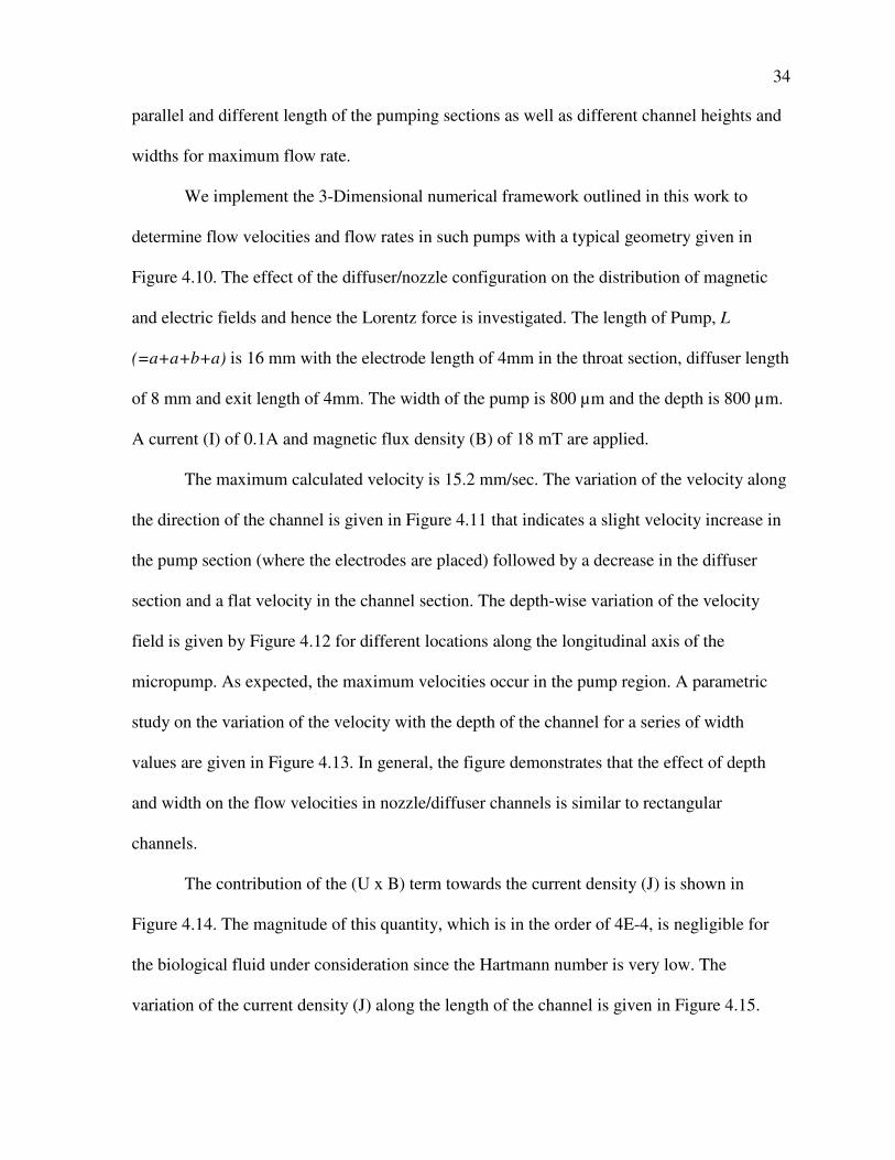
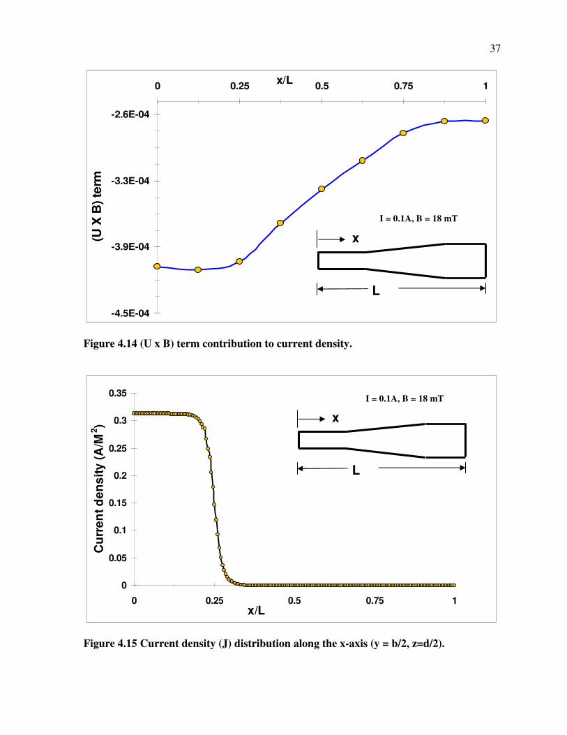
The contribution of the (U x B) term towards the current density (J) is shown in
Figure 4.14. The magnitude of this quantity, which is in the order of 4E-4, is negligible for
the biological fluid under consideration since the Hartmann number is very low. The
variation of the current density (J) along the length of the channel is given in Figure 4.15.

35
Figure 4.10 Geometry of nozzle/diffuser section.
8
9
10
11
12
13
14
15
16
0 0.25 0.5 0.75 1x/L
Velo
city (m
m/s
ec
)
Figure 4.11 Velocity distribution along the channel length of a nozzle-diffuser flow cell.
The velocity increases within the first 4 mm length (throat where the electrodes are
located) and then decreases in the diffuser section.
x
L
I = 0.1A, B = 18 mT

36
0.0
0.1
0.2
0.3
0.4
0 5 10 15
Velocity (mm/sec)
Depth
(m
m)
X=0.125L
x=0.25L
x=0.50L
x=0.75L
x=L
Figure 4.12 Velocity distributions in a nozzle-diffuser MHD flow-cell (depth and width
directions). In the depth direction, the flow is mainly pressure-driven by Lorentz force
and has the characteristics parabolic distribution.
0
3
6
9
12
15
0 0.5 1 1.5 2
Channel depth (mm)
Flo
w v
elo
city (m
m/s
ec)
width = 500 µµµµm
width = 800 µµµµm
width = 1000 µµµµm
L = 16 mm, Le = 4 mm
I = 0.1A, B = 18 mT
Figure 4.13 Dependence of velocity on depth in nozzle-diffuser shaped channels of
different widths.
x
L
I = 0.1A, B = 18 mT
37
-4.5E-04
-3.9E-04
-3.3E-04
-2.6E-04
0 0.25 0.5 0.75 1x/L
(U X
B) te
rm
Figure 4.14 (U x B) term contribution to current density.
0
0.05
0.1
0.15
0.2
0.25
0.3
0.35
0 0.25 0.5 0.75 1x/L
Cu
rre
nt
de
ns
ity
(A
/M2)
Figure 4.15 Current density (J) distribution along the x-axis (y = b/2, z=d/2).
x
L
x
L
I = 0.1A, B = 18 mT
I = 0.1A, B = 18 mT

38
Note that only the first 4 mm section of the pump has electrodes hence all the current density.
The current density decays to a zero value in the diffuser section. The effect of the diffuser
angle on the magnitude of the velocities is also investigated and a summary of the results
presented in Figure 4.16. For a given depth, a maximum velocity is obtained when the
diffuser angle (2θ) is about 5 degrees. This angle corresponds to a minimum frictional loss in
the channel. A similar value of 5 degrees has been reported by other researchers in valveless
diffuser pumps [45, 48].
4.2.3 Trapezoidal Channel
In typical silicon as well as glass micromachined channels, the MHD pump is
fabricated through a wet anisotropic etching of a V-groove through a silicon wafer [13, 32].
This results in a typical trapezoidal cross section of the flow channel with the side channels
assuming a typical angle of α = 54.7 degrees. The electrodes which are typically deposited on
the side walls are – therefore – non-parallel while the magnets are typically placed on the top
and bottom of the flow cell in a parallel fashion.
In the trapezoidal cross-section MHD pump example considered here, the length of
the channel is 4 mm, which is the same as length of electrode. The top width is 800 µm with
a bottom width of 230 µm and the depth of 400 µm. A constant voltage mode is assumed
here where instead of the current, the voltage is held constant. A potential of 1.5 volts is
applied at the anode whereas -1.5 volts is applied at the cathode. This approximately
corresponds to an average current of 0.01A. The magnitude of the magnetic flux density is
18 mT.

39
0.0
0.5
1.0
1.5
2.0
2.5
0 5 10 15Diffuser Angle (2θθθθ)
Lo
ren
tz F
orc
e -
N-m
Figure 4.16 Dependence of velocity on diffuser angle in nozzle-diffuser shaped channels.
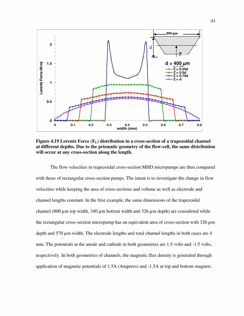
The current density distribution is given in Figure 4.17 whereas the magnetic flux
density is given in Figure 4.18. The two figures indicate that both the current density and the
magnetic flux density are not uniform at any given cross-section of the micropump with their
maximas typically occurring at the corners. The Lorentz force is non-uniform and in fact
assumes a “M’ shape distribution at the flow cell cross-sections as shown in Figure 4.19.
4.2.4 Trapezoidal vs. Rectangular Channel Selection
To compare and evaluate validity of trapezoidal channel cross section flow velocity, a
careful investigation between trapezoidal volume flow and rectangular volume flow rate has
been studies lately in research. Table 2.3 provides valid results to support the conclusion
about for given constant cross section area trapezoidal channel gives higher flow rate than
rectangular channel. This is also a proof the authentication of the conclusion.
2θ

40
0
5000
10000
15000
20000
25000
30000
0 0.1 0.2 0.3 0.4 0.5 0.6 0.7 0.8width (mm)
Curr
ent D
ensity (A
/M2)
Z = 0dZ = 0.25dZ = 0.5dZ = 0.75dZ = d
Figure 4.17 Current density (J/Area) distribution in a cross-section of a trapezoidal
channel at different depths. d is the depth of the channel. Due to the prismatic
geometry of the flow-cell, the same distribution will occur at any cross-section along the
length.
Figure 4.18 Streamlines of magnetic flux density in a trapezoidal shaped MHD pump.
In the middle region of the flow-cell, the magnetic flux density assumes uniform
magnitude and direction. However, due to the sloping sides, the magnetic flux is
distorted towards the sharp corners at the bottom of the flow-cell. The magnetic flux
density is also highest at the edges, A and B.
A B
Z
800 µµµµm
d
41
0
0.5
1
1.5
2
0 0.1 0.2 0.3 0.4 0.5 0.6 0.7 0.8
width (mm)
Lo
ren
tz F
orc
e (N
-m)
Z = 0dZ = 0.25dZ = 0.5dZ = 0.75dZ = d
Figure 4.19 Lorentz Force (FL) distribution in a cross-section of a trapezoidal channel
at different depths. Due to the prismatic geometry of the flow-cell, the same distribution
will occur at any cross-section along the length.
The flow velocities in trapezoidal cross-section MHD micropumps are then compared
with those of rectangular cross-section pumps. The intent is to investigate the change in flow
velocities while keeping the area of cross-sections and volume as well as electrode and
channel lengths constant. In the first example, the same dimensions of the trapezoidal
channel (800 µm top width, 340 µm bottom width and 326 µm depth) are considered while
the rectangular cross-section micropump has an equivalent area of cross-section with 326 µm
depth and 570 µm width. The electrode lengths and total channel lengths in both cases are 4
mm. The potentials at the anode and cathode in both geometries are 1.5 volts and -1.5 volts,
respectively. In both geometries of channels, the magnetic flux density is generated through
application of magnetic potentials of 1.5A (Amperes) and -1.5A at top and bottom magnets.
d
d = 400 µµµµm
Z
800 µµµµm

42
Table 2.4 Comparison of Flow Rate, Maximum Velocity and Lorentz’s Force in MHD
Micropumps of Trapezoidal and Rectangular Cross-Sections
Cross-section Max.
Velocity
(m/sec)
Current
Density
(A/m)
Magnetic Flux
Density (B)
Lorentz’s
Force
(N-m/m)
Flow Rate (Q)
µliter/min
Trapezoidal
top width = 800 µm,
bot. width = 340 µm
depth = 326 µm
1.86e-3 0.001467 1.86e-9 1.60e-5 9.05
Rectangular
width = 570 µm
depth = 326 µm
1.69e-3 0.001467 2.10e-9 1.66e-5 9.25
Trapezoidal
top width = 1000 µm,
bot. width = 575 µm
depth = 350 µm
1.65e-3 0.00157 2.57e-9 1.61e-5 11.73
Rectangular
width = 787.5 µm
depth = 350 µm
1.54e-3 0.00157 2.84e-9 1.69e-5 12.25
Note: Channel length as well as electrode lengths are 4 mm.
The solution of the full 3D MHD equations for both trapezoidal and rectangular
cross-section MHD micropumps is then carried out under these equivalent conditions for all
the physics under consideration. Table 2.4 summarizes the results in maximum velocity, flow
rate, Lorentz’s force, magnetic flux density and current at a cross-section taken at half-length
of the micropumps. Our results indicate that the flow rate in trapezoidal cross-section
micropumps is comparable to that of rectangular cross-section pumps unlike the results
reported by like Bao and Harrison [37] who used an approximate formula for macro
channels to report differences as high as a factor of 3. The results from this analysis which is
based on rigorous accounting of all the multi-physics in MHD micropumps, therefore,
demonstrate for the first time that trapezoidal cross-section micropumps offer as good flow
43
rate as rectangular cross-sections. Table 2.2 also shows that the maximum velocity evaluated
in trapezoidal micropumps is slightly higher than those in rectangular micropumps. In the
dimensions considered here, the variations were between 7-10%. On the other hand, the flow
rates in rectangular micropumps are evaluated to be slightly higher than those of trapezoidal
cross-section micropumps. The variations are, however, less than 5% for the dimensions
considered suggesting that trapezoidal cross-section MHD micropumps which are easy to
micromachine (Lemoff and Lee, 2000) are as efficient as rectangular MHD micropumps.
Further, Table 2.2 summarizes that the total net current and magnetic flux densities at a given
cross-section of these micropumps are comparable with their differences being less than 10%
in the case of magnetic flux density and nil in the case of total current. The Lorentz’s force –
which is a direct function of the magnetic flux density and current density - is, therefore, of
comparable magnitude in both rectangular and trapezoidal cross-section micropumps.
44
CHAPTER 5
DISCUSSION OF EO AND JOULE EFFECT
5.1 ELECTROOSMOSIS
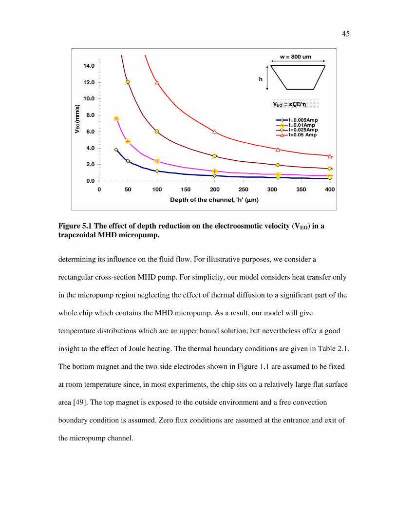
The effect of electroosmosis on the fluid flow pattern and magnitude is investigated
next. For this electroosmotic study, we have used MHD pump of trapezoidal cross-section
geometry with width of 800 µm, depth of 380 µm, electrode length of 4 mm, and total
channel length of 20 mm. The current used is 0.01A with magnetic flux density of 18 mT and
zeta potential of 0.1V. The main Lorentz’s flow in this geometry of MHD pump was found to
be about 0.5 mm/sec. The electroosmotic velocity (VEO), on the other hand, is evaluated by
the Helmholtz-Smoluchowski Equation (Eqn 4) to be 0.6 mm/sec – the same order as the
main flow for this particular current density. The effect of scaling of the depth on
electroosmotic velocity is studied by varying the depth from 400 µm down to 30 µm.
Figure 5.1 shows that the electroosmotic velocity increases quadratically with the decrease in
the depth of the channel as is the case for rectangular MHD pumps. For current levels of only
0.025A, electroosmotic velocity of as much as 3.0 mm/sec is predicted for channel depth of
200 um. For smaller depths such as 30 um, the electroosmotic velocity increases to as much
as 7.6 mm/sec for a current of 0.01A.
5.2 EFFECT OF JOULE HEATING AND VISCOSITY UNDER
TEMPERATURE CHANGES
One of the main physics considered here is that of Joule heating with the objective of
45
0.0
2.0
4.0
6.0
8.0
10.0
12.0
14.0
0 50 100 150 200 250 300 350 400
Depth of the channel, 'h' (µµµµm)
VE
O (m
m/s
)
I=0.005AmpI=0.01AmpI=0.025AmpI=0.05 Amp
VEO = ε ζΕ/ ηε ζΕ/ ηε ζΕ/ ηε ζΕ/ η
w = 800 um
h
Figure 5.1 The effect of depth reduction on the electroosmotic velocity (VEO) in a
trapezoidal MHD micropump.
determining its influence on the fluid flow. For illustrative purposes, we consider a
rectangular cross-section MHD pump. For simplicity, our model considers heat transfer only
in the micropump region neglecting the effect of thermal diffusion to a significant part of the
whole chip which contains the MHD micropump. As a result, our model will give
temperature distributions which are an upper bound solution; but nevertheless offer a good
insight to the effect of Joule heating. The thermal boundary conditions are given in Table 2.1.
The bottom magnet and the two side electrodes shown in Figure 1.1 are assumed to be fixed
at room temperature since, in most experiments, the chip sits on a relatively large flat surface
area [49]. The top magnet is exposed to the outside environment and a free convection
boundary condition is assumed. Zero flux conditions are assumed at the entrance and exit of
the micropump channel.

46
The dependency of viscosity and conductivity on temperature are accounted for using
Equations 6 and 7.
2273
003.7273
306.5704.1ln
+
−−=
TToη
η
σT = σ (1+0.02T)
where σ is viscosity in N-sec/m2, σT is viscosity at room temperature and T is temperature
in degree Kelvin. Note that Equation 1 which is applicable for water is extended for use for
the biological electrolyte considered in this study by using a proportionality factor of 0.6 to
account for the ratio of viscosity of water to 1M saline solution at room temperature. The
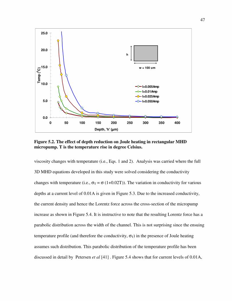
thermal boundary conditions are given in Table 2.1. Figure 5.2 shows the range of
temperature changes predicted in a rectangular MHD micro-pump discussed in section 3.1.
The figure shows that temperature increases as much as 20 OC and more are possible in
rectangular cross-section MHD pumps for channels of depths of 30 µm and width of 100 µm
when subjected to a current of 0.025A. The Joule heating is, of course, a function of J2/σ
(Eq. 5.a); therefore significant temperature rises are predicted for micropumps with increased
current densities as in shallow channels. Given the fact that the conductivity of most
biological electrolytes increases by 2% for each degree rise in temperature [41], the 20 OC
rise in temperature in shallow rectangular channels reported here can effectively increase the
fluid conductivity locally by as much as 40%. This will in turn lead to increases in current
strength and hence Lorentz’s force and fluid flow velocity in MHD micropumps. The fluid
velocity is also further increased by a decrease in viscosity. Analysis was carried where the
full 3D MHD equations developed in this study were solved considering the conductivity and
47
0.0
5.0
10.0
15.0
20.0
25.0
0 50 100 150 200 250 300 350 400
Depth, 'h' (µµµµm)
Tem
p (
0C
)
I=0.005Amp
I=0.01Amp
I=0.025Amp
I=0.050Amp
w = 100 um
h
Figure 5.2. The effect of depth reduction on Joule heating in rectangular MHD
micropump. T is the temperature rise in degree Celsius.
viscosity changes with temperature (i.e., Eqs. 1 and 2). Analysis was carried where the full
3D MHD equations developed in this study were solved considering the conductivity
changes with temperature (i.e., σT = σ (1+0.02T)). The variation in conductivity for various
depths at a current level of 0.01A is given in Figure 5.3. Due to the increased conductivity,
the current density and hence the Lorentz force across the cross-section of the micropump
increase as shown in Figure 5.4. It is instructive to note that the resulting Lorentz force has a
parabolic distribution across the width of the channel. This is not surprising since the ensuing
temperature profile (and therefore the conductivity, σT) in the presence of Joule heating
assumes such distribution. This parabolic distribution of the temperature profile has been
discussed in detail by Petersen et al [41] . Figure 5.4 shows that for current levels of 0.01A,

48
1.45
1.50
1.55
1.60
1.65
1.70
1.75
1.80
0 2 4 6 8 10
Length of the Channel (mm)
Conductivity (S
/m)
25 micron depth
35 micron depth
50 micron depth
L = 11 mm
I = 0.01 Amp
B = 18 mT
Figure 5.3 The variation of conductivity of electrolyte along the centerline of MHD
pump of rectangular cross-section due to Joule heating.
0
1
2
3
4
5
0 0.125 0.25 0.375 0.5
y/Width (µµµµm)
Lore
ntz
Forc
e (N
-m)
I=0.01 AI=0.015 AI=0.02 AI=0.01 A (No Joule Heating)
y
width
Figure 5.4 The effect of Joule heating on the Lorentz’s force in rectangular MHD
micropump. The Lorentz force is calculated at the center of the pump.
pump region
49
0.015A, and 0.025A, the average increases in the Lorentz force in the pump section are 20%,
30% and 44%, respectively. Further, decreases in viscosity of as much as 20% for channel
depths of 50 µm and width of 100 µm under a current of 0.025A were observed due to Joule
heating which in turn contribute to a proportional increase in flow velocity. The results from
this study, therefore, suggest that the effects from Joule heating could be significant enough
to warrant consideration, particularly for shallow MHD micropumps where the current
densities are high.

50
CHAPTER 6
CONCLUSION
In this thesis a complete numerical framework for the three-dimensional MHD
equations that govern the behavior of MHD micropumps is developed. This is expected not
only to fill the gap that has existed for sometime now in the area of prediction and
optimization of the behavior of such micropumps under differing geometric configurations,
electric fields and magnetic flux densities but also provide a useful analytical tool to
investigate newer configurations and designs. Our research indicates that:
Transverse electroosmotic flows could have a considerable effect on the efficiency of
axial MHD pumps especially for MHD micro-pumps with shallow channels and high current
density. In some cases, the electroosmotic velocity could be significantly higher than the
main Lorentz flow. Electroosmotic flow in a high current density DC MHD pump was
experimentally observed and reported by Homsy et al. [39]. This current study is, however,
the first work that uses rational analytical expressions to predict this flow.
Joule heating has a significant effect on the flow velocity of MHD micropumps,
especially for pumps with shallow depths and higher current density. As much as 20oC
increase in the temperature of the electrolyte are predicted for high current densities. Again,
Joule heating has been experimentally observed by Homsy et al. (2005) [39]. Our work is the
first to quantify this heating.
Joule heating is observed to in-turn increase the conductivity but decrease the
viscosity of the electrolyte. The increase in electrolyte conductivity in turn translates to
51
increased current densities and hence Lorentz forces and flow velocity. The decrease in the
electrolyte viscosity also leads to increased flow velocity.
In almost all the research reported in MHD micro-pumps, the magnetic and electric
fields are assumed to be uniform. However, due to the non-alignment of the magnets with the
electrodes and defects in the geometry of the channels during anisotropic etching of (100)
silicon, the electric and magnetic fields may not be always uniform and symmetrical. Further,
when the electrode material is deposited on the side of the channel, it may result in non-
parallel electrodes [37] which in turn could cause non-uniform electric fields. The 3D
numerical framework developed in this study, therefore, provides a useful tool to model such
non-uniformities.
This work is also the first to report solution of the 3D MHD equations in the case of
MHD pumps with trapezoidal cross-sections. Our work provides a more rational and
thorough numerical framework for micropumps of arbitrary cross-sections than previous
approximate results reported by Bao and Harrison [37] who investigated fluid velocities and
flow rates for rectangular and trapezoidal sections using a simple Poiseuille type
approximations.
Numerical results reported here demonstrate that for an equivalent area of cross
section and electrode length as well as current and magnetic flux densities, a trapezoidal
cross-section MHD micropump could indeed give a comparable flow rate as that of
rectangular cross-section MHD micropumps. Bao and Harrison [37] had used approximate
formula applicable to macro channels under pressure-driven flows to report that trapezoidal
cross-section MHD micropumps provided only one-third of the mean flow velocity and flow
rate offered by rectangular cross-section micropumps. We think the major flaw in the

52
approximate formula used arise from the inability of the model to take into account the effect
of geometry on the variation of current and magnetic flux density at a cross-section. Only a
model based on a full geometric descetization and solution of the most general MHD
equations can predict these variations. It turns out that while there are significant local
variations of the current and magnetic flux densities, the total integrated quantities at a given
cross-section for both rectangular and trapezoidal cross-sections are comparable. The
obvious implication of these results in flow rates is that trapezoidal cross-section MHD
micropumps which are easier to micromachine through wet anisotropic etching of silicon
than rectangular cross-section micropumps have a competitive advantage.
The increased miniaturization of MHD micropumps to the range of tens of microns of
characteristics dimensions that is being pursued by the research community [37], [45] where
the validity of continuum-based equations becomes questionable suggests that there still
remains the need for extending the computational frameworks developed here and elsewhere
to accommodate such miniaturizations.

53
REFERENCES
[1] S. Shoji, M. Esashi, Microflow devices and systems, J. Micromech. Microeng.
4(1994) 157-171
[2] R. Zengerle, J. Ulrich, S. Kluge, M. Richter, A. Richter, A bidirectional silicon
micropump, Sensors and Actuators A 50 (1995) 81-86
[3] M.J. Zdeblick, R. Anderson, J. Jankowski, B. Kline-Schoder, L. Christel, R. Miles,
W. Weber, in: Thermopneumetically Actuated Microvalves and Integrated Electro-
Fluidic Circuits, Solid-State Sensors and Actuator Workshop, Hilton Head, SC, June
13-16, 1994, pp. 251-255.
[4] J. Branebjerg, B. Fabius, P. Gravesen, Application of miniature analyzers: From
microfluidic components to mTAS, in: A. van den Berg, P. Bergfeld, Eds..,
Proceedings of Micro Total Analysis Systems Conference, Twente, Netherlands,
Nov. 21–22, 1994, pp. 141–151.
[5] H.T.G. van Lintel, F.C.M. van de Pol, S. Bouwstra, A piezoelectric micro pump
based on micromachining of silicon, Sensors and Actuators 151988.153
[6] R.M. Moroney, R.M. White, R.T. Howe, Ultrasonically induced microtransport, in:
Proceedings of the IEEE 1991 Micro Electro Mechanical Systems Workshop MEMS
’91., Nara, Japan, Jan. 30–Feb. 2, 1991, pp. 277–282
[7] W. Zhang, C.H. Ahn, in: A Bi-Directional Magnetic Micropump on a Silicon
Wafer,Solid-State Sensor and Actuator Workshop, Hilton Head, SC, 1996, p. 94.
[8] S.E. Mc Bride, R.M. Moroney, W. Chiang, Electrohydrodynamic pumps for high-
density microfluidic arrays, in: D.J. Harrison, A. vanden Berg Eds.., Proceedings of
Micro Total Analysis Systems Conference, Banff, Canada, Oct. 13–16, 1998,
pp. 45–48.
[9] A. Manz, C.S. Effenhauser, N. Burggraf, D.J. Harrison, K. Seiler, K. Flurri,
Electroosmotic pumping and electrophoretic separations for miniaturized chemical
analysis systems, Journal of Micromechanics and Microengineering 4 1994.257–265.
[10] P.H. Paul, D.W. Arnold, D.J. Rakestraw, Electrokinetic generation of high pressures
using porous microstructure, in: D.J. Harrison, A. van den Berg Eds.., Proceedings of
Micro Total Analysis Systems Conference, Banff, Canada, Oct. 13–16, 1998,
pp. 49–52.

54
[11] A. Richter, A. Plettner, K.A. Hofmann, H. Sandmaier, A microma- chined
electrohydrodynamic EHD.pump, Sensors and Actuators A 29 1991.159–168.
[12] T.K. Jun, in: Microscale pumping with traversing bubbles in microchannels, Solid-
State Sensor and Actuator Workshop, Hilton Head, SC, 1996, p. 144.
[13] Lemoff, A.V., Lee, A.P., 2000. An AC magnetohydrodynamic micro-pump, Sensors
and Actuators B, 63, pp178–185.
[14] W. Ritchie, Experimental researches in voltaic electricity and electromagnetism,
Philos. Trans. R. Soc. London 122 1832.279–298.
[15] Hughes, M., Pericleous, K.A., Cross, M., 1995, The Numerical Modeling of DC
Electromagnetic Pump and Brake Flow, Appl. Math. Model 19, pp713-723.
[16] Ramos, J.I., Winowich, N.S., 1990, Finite Difference and Finite Element Methods for
MHD Flows, Int. J. Numerical Methods in Fluids, Vol. 11, pp907-934.
[17] Winowich, N.S., Hughes, W. F., Ramos, J.I., 1987, Numerical Simulation of
Electromagnetic Pump Flow, Numerical Methods in Laminar Turbulent Flow, 5 (2),
pp1228-1240.
[18] Hunt, J.C.R and Stewartson, K. – Magnetohydrodynamic Flow in Rectangular Ducts
II J. Fluid Mech., Vol. 23, part 3, pp. 563-581, 1965.
[19] Hughes, W.F, and McNAB, I.R. – A Quasi- One Dimensional Analysis of an
Electromagnetic Pump Including End Effects. Liquid-Metal Flows and
magnetohydrodynamics, Eds. Branover, H., Lykoudis, P.S, and Yakhot, A., Progress
in Astronautics and Aeronautics, Vol. 84, pp. 287-312, AIAA, New York, 1983.
[20] Hughes W.F. and Young F. J. (1966) The electromagnetoydrodynamics of Fluid,
John Wiley & Sons, New York.
[21] Turner R.B. (1973) “ Aspect of MHD duct flow at high magnetic Reynolds number,”
PhD Thesis, Univ. of Warwick, England.
[22] Walker J.S. and Ludford G.S.S. (1974) “ MHD flow in insulating circular expansions
with strong transvers magnetic fields.” Int. J. Eng. Sci. , Vol. 12. pp. 1045-1061
[23] Holroyd E.T. and Hunt J.C.R (1976) “ A review of MHD flows in ducts with
changing cross section areas and non-uniform magnetic fields,” Euromech
Colloquium 70, March 16-19.
[24] Branover H. (1974) “On some important effects in laboratory MHD flows in
rectangular ducts in transverse magnetic fields”. Proc. 14th conf. Eng. Aspects of
MHD, Tullahoma, Tenn.

55
[25] Branover H. and Gershon P. (1976) “ MHD turbulence study, ” Ben-guroin
University, Rept. BGUN-RDA-100-76.
[26] Singh, B., and Lal, J., Finite element problems in magnetohydrodynamics and
channel flow problems, International Journal of Num. Methods in Engineering, 1982,
15, pp1104.
[27] WINOWICH, N.S. and HUGHES, W. F. – A Finite Element Analysis of Two-
dimensional MHD Flow. Liquid-Metal flows and magnethydrodynamics, Eds.
Branover, H., Lykoudis, P.S., and Yakhot, A., Progress in Astronautics and
Aeronautics, Vol. 84, pp. 313-322, AIAA, New York, 1983.
[28] G. Yagawa and M. Masuda, “ Finite element analysis of magnetohydrodynamics and
its application to lithium blanket design of fusion reactor. Nucl. Eng. Design, 71,
121-136 (1982).
[29] Winowich, N.S., Hughes, W.F., Ramos, J.I., 1987, Numerical Simulation of
Electromagnetic Pump Flow, Numerical Methods in Laminar Turbulent Flow, 5 (2),
pp1228-1240.
[30] J. I. Ramos and N. S. Winowich, “Magnetohydrodynammic channel flow study”,
Phys. Fluids, 29(4), 992-997 (1988)
[31] Ramos, J.I., Winowich, N.S., 1990, Finite Difference and Finite Element Methods for
MHD Flows, Int. J. Numerical Methods in Fluids, Vol. 11, pp907-934.
[32] Jang, J., Lee, S.S., 2000. Theoretical and experimental study of MHD micro-pump.
Sensors and Actuators A 80, pp84–89.
[33] Huang, L., Wang, W., Murphy, M.C., 1999. A lumped-parameter model for a micro-
pump based on the magnetohydrodynamic (MHD) principle. Proc. SPIE–Design Test
Microfabric. MEMS MOEMS 3680, pp379–387.
[34] Huang, L., Wang, W., Murphy, M.C., Lian, K., Ling, Z.G., 2000. LIGA fabrication
and test of a DC type magneto-hydrodynamic (MHD) micro-pump. Microsyst.
Technol. 6, pp235–240.
[35] Heng, K.H., Huang, L., Wang, W., Murphy, M.C., 1999. Development of a
diffuser/nozzle type micro-pump based on magnetohydrodynamic (MHD) principle.
Proc. SPIE—Microfluidic Devices Systems, II, 3877, pp66–73.
[36] Heng, K.H., Wang, W., Murphy, M.C., Lian, K., 2000. UV-LIGA microfabrication
and test of an ac-type micro-pump based on the magnetohydrodynamic (MHD)
principle. Proc. SPIE—Microfluidic Dev. Syst. III, 4177, pp174–184.
[37] Bao, JB., and Harrison, D.J., 2003. Fabrication of microchips for running liquid
chromatography by magnetohydrodynamic flow, 7th lnternational Conference on

56
Miniaturized Chemical and Biochemical Analysts Systems, Squaw Valley, California
USA.
[38] Wang, P.J., Chang, C.Y., and Chang. M.L., 2004, “ Simulation of two-dimensional
fully developed laminar flow for a magneto-hydrodynamic (MHD) pump”,
Biosensors and Bioelectronics, 20, pp115-121.
[39] Homsy, A, Koster, S, Eijkel, JCT, Berg, A, Lucklum, F, Verpoorte, E, and de Rooij,
NF, 2005, A high current density DC magnetohydrodynamic (MHD) micropump,
Lab Chip, 5(4), pp466-471.
[40] Probstein, R.F., 1994, Physicochemical Hydrodynamics, An Introduction, Wiley &
Sons, New York.
[41] Petersen, N.J., Nikolajsen, R.P.H., Mogensen, K.B., Kutter, J.P., 2004, Effect of Joule
heating on efficiency and performance for microchip-based and capillary-based
electrophoretic separation systems: A closer look, Electrophoresis 2004, 25,
pp. 253–269.
[42] Ramos, A., Morgan, H., Green, N.G., and Castellanos, A., 1998, AC electronics: a
review of forces in microelectrode structures, J. Phys. D: Appl. Phys. 31, pp2338-
2353.
[43] Tillack, M.S., and Morley, N.B., 1998, Magnetohydrodynamics, Standard Handbook
for Electrical Engineers, McGraw Hill, 14-th Edition.
[44] FEMLAB FEA Software, Reference Manual, version 3.1, COMSOL, Inc., 2005.
[45] Lee, A.P., 2005, personal communications.
[46] Olsson, A., Enoksson, P., Stemme, G., and Stemme, E., 1997. Micromachined flat-
walled valveless diffuser pumps, Journal of MEMS, Vol. 6, pp161–166.
[47] Heschel, M., Mullenborn, M., Bouwstr, S., 1997, Fabrication and characterization of
truly 3-D diffuser/nozzle microstructures in silicon, Journal of
Microelectromechanical Systems, pp41-47.
[48] Bendib, S., Français, O., 1999, Analytical study of microchannel and passive
microvalve application to micropump simulator, Proc. SPIE, pp 200-208.
[49] Erickson, D., Sinton, D., Li, D., 2003, Joule Heating and Heat Transfer in
Poly(dimethylsiloxane) Microfluidic Systems, Lab on a Chip, 3, pp 141-149.
[50] M. Hughes, K.A. Pericleous, M. Cross, The numerical modeling of dc 672
electromagnetic pump and brake flow, Appl. Math. Model 19 (1995) 673 713–723.
674.

57
[51] J.I. Ramos, N.S. Winowich, Finite difference and finite element methods for MHD
flows, Int. J. Numer. Meth. Fluids 11 (1990) 907–934. 676.
[52] N.S. Winowich, W.F. Hughes, J.I. Ramos, Numerical simulation of electromagnetic
pump flow, Numer. Meth. Laminar Turbulent Flow 5 (2) 678 (1987) 1228–1240.

ABSTRACT OF THE THESIS
Electroosmosis and Thermal Effects in Magnetohydrodynamic (MHD)
Micropumps Using 3D MHD Equations
by
Vaibhav D. Patel
Masters of Science in Mechanical Engineering
San Diego State University, 2007
Magnetohydrodynamics (MHD) is a phenomenon observed in electrically conductive
liquid in the presence of a magnetic field where a body force called “Lorentz Force” is produced.
Based on this MHD physics, MHD micropumps are increasingly being used for pumping
biological and chemical specimens such as blood and saline buffers. This research reports the
development of generalized 3D MHD equations that govern the multiphysics of micropumps.
Based on the solution of the numerical framework developed, the thesis reports effect such as
non uniform magnetic and electric fields, Joule Heating, electroosmosis, pinch effect and M
shaped velocity profile in different flow channel geometries.