multimodal transportation for perishable products - tu/e · multimodal transportation for...
TRANSCRIPT

Multimodal transportation for perishable products
Citation for published version (APA):Steadie Seifi, M. (2017). Multimodal transportation for perishable products. Eindhoven: Technische UniversiteitEindhoven.
Document status and date:Published: 21/03/2017
Document Version:Publisher’s PDF, also known as Version of Record (includes final page, issue and volume numbers)
Please check the document version of this publication:
• A submitted manuscript is the version of the article upon submission and before peer-review. There can beimportant differences between the submitted version and the official published version of record. Peopleinterested in the research are advised to contact the author for the final version of the publication, or visit theDOI to the publisher's website.• The final author version and the galley proof are versions of the publication after peer review.• The final published version features the final layout of the paper including the volume, issue and pagenumbers.Link to publication
General rightsCopyright and moral rights for the publications made accessible in the public portal are retained by the authors and/or other copyright ownersand it is a condition of accessing publications that users recognise and abide by the legal requirements associated with these rights.
• Users may download and print one copy of any publication from the public portal for the purpose of private study or research. • You may not further distribute the material or use it for any profit-making activity or commercial gain • You may freely distribute the URL identifying the publication in the public portal.
If the publication is distributed under the terms of Article 25fa of the Dutch Copyright Act, indicated by the “Taverne” license above, pleasefollow below link for the End User Agreement:
www.tue.nl/taverne
Take down policyIf you believe that this document breaches copyright please contact us at:
providing details and we will investigate your claim.
Download date: 03. Jan. 2020
Multimodal Transportationfor Perishable Products
Maryam SteadieSeifi

Printed and cover design by Proefschriftmaken.nl || Uitgeverij BOXPress
This thesis is number D206 of the thesis series of Beta Research School for OperationsManagement and Logistics. Beta Research School is a joint effort of the School ofIndustrial Engineering and the Department of Mathematics and Computer Scienceat Eindhoven University of Technology, and Center for Production, Logistics andOperations Management at the University of Twente.
A calatogue record is available from the Eindhoven University of Technology Library.
ISBN: 978-94-6295-581-3
This research has been partially funded by the Top consortium Knowledge andInnovation - Dutch Institute for Advanced Logistics (TKI-Dinalog), under the projecttitled DaVinc3i, #2010.2.034R.

Multimodal Transportation
for Perishable Products
PROEFSCHRIFT
ter verkrijging van de graad van doctor aan de Technische UniversiteitEindhoven, op gezag van de rector magnificus prof.dr.ir. F.P.T. Baaijens,voor een commissie aangewezen door het College voor Promoties, in het
openbaar te verdedigen op donderdag 21 maart 2017 om 16:00 uur
door
Maryam SteadieSeifi
geboren te Teheran, Iran
Dit proefschrift is goedgekeurd door de promotoren en de samenstelling van depromotiecommissie is als volgt:
voorzitter: prof.dr. I.E.J. Heynderickx1e promotor: prof.dr. T. van Woenselcopromotor(en): dr.ir. N. Dellaertleden: prof.dr.ir. R. Dekker (Erasmus University of Rotterdam)
prof.dr. A.G. de Kokprof.dr. J. Hurink (University of Twente)prof.dr.ir. W. Nuijten
Het onderzoek of ontwerp dat in dit proefschrift wordt beschreven is uitgevoerd inovereenstemming met de TU/e Gedragscode Wetenschapsbeoefening.

Acknowledgments
I would like to first thank my promoter Tom van Woensel for opening the rabbit holeand letting me experience a wonderland, academically, professionally, socially, andpersonally. Tom, I am grateful for the time you spent on reviewing my work andgiving me substantial feedback during these years. I am also grateful for your lessonsto make me a more confident, self-reliant, and pragmatic professional.
The next person I have to express my sincere appreciation is my co-promoter anddaily supervisor, Nico Dellaert. Nico, you have been a great mentor to me, and Ienjoyed all our conversations and discussions, both scientific and general, especiallyin the last two years of my PhD. Your comments and feedback have enhanced myknowledge and comprehension.
I would also like to thank Wim Nuijten, my advisor during the initial steps of theresearch. Wim, your academic and business experience both helped me furtherdevelop my problem solving mindset. I appreciate the time you then spent reviewingmy work, and for your detailed and constructive feedback.
Tom, Nico, Wim, and my dear friend Rasa, we wrote a literature review paper togetherwhich gained a lot of attention and even won a prize. When I look back at the wholeprocess of writing and editing it until the EURO2016 conference where we receivedthe award, I find it an amazing, unexpected, and joyful experience. So, thank you allfor this fruitful and memorable collaboration.
To Ton de Kok, Johann Hurink, and Rommert Dekker, I would like to express myappreciation for accepting to be a part of my thesis committee. Thank you for yourvaluable comments, which have significantly improved the quality of my work. Ton,you were also one of the key people in hiring me for this PhD position, so, I furtherthank you for that.
Next, I would like to thank the people in DAVINC3I project who brought practicalviewpoint into my work. In particular, I have to thank Edwin Wenink, Rob Koppes,Robbert van Willegen, and Marlies de Keizer. Being a part of this project was myfirst international work experience and I am happy that I was a part of it.
v

I would like to thank all my former and current OPAC colleagues, especially my PhDand PostDoc fellows. I like to especially thank the following people, with whom I hada great time and valuable knowledge exchange, and shared lots of memories: Anna,Said, Derya, Hande, Ben, Kristina, Kasper and Marija, Frank, Joachim, Maximilianoand Heather, Qiushi, Chiel, Stefano, Hao, Peng, Baoxiang, Veaceslav, Qianru, Jose,Ayse, Dmitry, Engin and Ipek, Giro, Joost, Joni, Sjors, Laura, Denise, Loe, Bram,Afonso, and my successor, Erwin. Moreover, I have to sincerely thank Mark Stobbefor enhancing my JAVA and object-oriented programming skills. Furthermore, toOPAC secretaries, especially Jose van Dijk-Kok, Jolanda Verkuijlen-Nelissen, andClaudine Hulsman-Paul, I am grateful for all your assistance and help.
My dear Iranian colleagues, Shaya, Taimaz, Yousef, Fardin, Taher, and Alireza, havingyou as colleagues was a blessing. We had lots of fun at work, but I am especiallythankful for your support during the occasions I felt helpless. I think without youguys, I would have probably gone mad. Among my other amazing Iranian friends,Nooshin, Ghazaleh, Farnaz, Tahoora, Raheleh, Mona, Rasa, Sina, Danial (and thewhole family), Ehsan, Mehdi, Helen, Reihaneh, Fereshteh and Hani, thank you forall the laughter and memories you shared with me. Among the many wonderfulexpats and Dutch people I have met during these years, I like to especially thankDeepak, Marie-Jose, and Marcel, for all the amazing adventures and experiences wehad together.
Finally, Maman, Baba, and my lovely family, there is absolutely no phrase showinghow much I feel thankful to have you in my life. Baba, you supported me in all thedecisions I made in my life, and always encouraged me to do better. This PhD is theresult of your support and I am indebted to you. Maman, you are my role model andguardian angel, whether close or far. I am always appreciative for your unconditionallove, cheering, and embrace. Haydeh, I love you as my big sister, and I thank you foryour presence and support. Omid, my dadashi, thank you for being there for Mamanand Baba during the times they needed my help and company. I hope I can in returnhelp you fulfill your dreams.
Maryam SteadieSeifiNorouz 2017

to my dad,
to my mom,
and to my lovely family.

Contents
I Opening 1
1 Introduction 31.1 Motivation and Challenges . . . . . . . . . . . . . . . . . . . . . . . . . 41.2 Perishability in Transportation Planning Literature . . . . . . . . . . . 81.3 Transportation Planning Problems and Scope of Thesis . . . . . . . . 111.4 Research Objectives . . . . . . . . . . . . . . . . . . . . . . . . . . . . 121.5 Outline of Thesis and its Contribution . . . . . . . . . . . . . . . . . . 14
2 Multimodal Freight Transportation: A Literature Review onTactical and Operational Planning 172.1 Multimodal Transportation . . . . . . . . . . . . . . . . . . . . . . . . 182.2 Tactical Planning Problems . . . . . . . . . . . . . . . . . . . . . . . . 202.3 Operational Planning Problems . . . . . . . . . . . . . . . . . . . . . . 322.4 Prospectives . . . . . . . . . . . . . . . . . . . . . . . . . . . . . . . . . 38
II Tactical Planning 41
3 A MIP for Multimodal Long-haul Transportation of PerishableProducts with Empty Repositioning 433.1 Problem Description . . . . . . . . . . . . . . . . . . . . . . . . . . . . 433.2 Related Literature . . . . . . . . . . . . . . . . . . . . . . . . . . . . . 463.3 Modeling Approach . . . . . . . . . . . . . . . . . . . . . . . . . . . . . 47
3.3.1 Mode-Space-Time Network Representation . . . . . . . . . . . 473.3.2 Modeling Quality Preservation . . . . . . . . . . . . . . . . . . 50
3.4 Mathematical Model . . . . . . . . . . . . . . . . . . . . . . . . . . . . 503.5 Numerical Experiments . . . . . . . . . . . . . . . . . . . . . . . . . . 56
3.5.1 Instance Sets . . . . . . . . . . . . . . . . . . . . . . . . . . . . 563.5.2 Computational Strengthening . . . . . . . . . . . . . . . . . . . 583.5.3 Results . . . . . . . . . . . . . . . . . . . . . . . . . . . . . . . 58
3.6 Conclusions . . . . . . . . . . . . . . . . . . . . . . . . . . . . . . . . . 61
4 An ALNS Metaheuristic for Multimodal Long-haul Transporta-tion of Perishable Products with Empty Repositioning 63
ix
4.1 Problem Description . . . . . . . . . . . . . . . . . . . . . . . . . . . . 644.2 Related Literature . . . . . . . . . . . . . . . . . . . . . . . . . . . . . 654.3 Solution Algorithm . . . . . . . . . . . . . . . . . . . . . . . . . . . . . 66
4.3.1 Construction of an Initial Solution . . . . . . . . . . . . . . . . 684.3.2 Neighborhoods and Operators . . . . . . . . . . . . . . . . . . . 714.3.3 The First Adaptive Neighborhood Search (ANS-1) . . . . . . . 734.3.4 Long-term Memory and the Second Adaptive Neighborhood
Search (ANS-2) . . . . . . . . . . . . . . . . . . . . . . . . . . . 774.4 Computational Results . . . . . . . . . . . . . . . . . . . . . . . . . . . 77
4.4.1 Parameter Tuning . . . . . . . . . . . . . . . . . . . . . . . . . 784.4.2 Overall Results . . . . . . . . . . . . . . . . . . . . . . . . . . . 784.4.3 Algorithm Performance . . . . . . . . . . . . . . . . . . . . . . 804.4.4 Incomplete Transportation Network . . . . . . . . . . . . . . . 84
4.5 Conclusions . . . . . . . . . . . . . . . . . . . . . . . . . . . . . . . . . 85
III Operational Planning 87
5 A Rolling Horizon Framework for Operational Planning of Long-haul Transportation of Perishable Product 895.1 Problem Description . . . . . . . . . . . . . . . . . . . . . . . . . . . . 895.2 Related Literature . . . . . . . . . . . . . . . . . . . . . . . . . . . . . 925.3 Modeling Approach . . . . . . . . . . . . . . . . . . . . . . . . . . . . . 945.4 Rolling Horizon Framework . . . . . . . . . . . . . . . . . . . . . . . . 97
5.4.1 State of System and Roll Solution . . . . . . . . . . . . . . . . 985.4.2 ALNS and Planning Process . . . . . . . . . . . . . . . . . . . 99
5.5 Computational Results . . . . . . . . . . . . . . . . . . . . . . . . . . . 1015.5.1 Overall Results . . . . . . . . . . . . . . . . . . . . . . . . . . . 1025.5.2 The Length of a Roll . . . . . . . . . . . . . . . . . . . . . . . . 1045.5.3 Partial versus Complete Reoptimization . . . . . . . . . . . . . 1045.5.4 The End of Week RTI Repositioning . . . . . . . . . . . . . . . 105
5.6 Conclusions . . . . . . . . . . . . . . . . . . . . . . . . . . . . . . . . . 105
6 A Scenario-based Stochastic Rolling Horizon Framework for Op-erational Planning with Demand Uncertainty 1076.1 Problem Description . . . . . . . . . . . . . . . . . . . . . . . . . . . . 1086.2 Related Literature . . . . . . . . . . . . . . . . . . . . . . . . . . . . . 1126.3 Modeling Approach and Solution Algorithm . . . . . . . . . . . . . . . 115
6.3.1 Rolling Horizon Framework . . . . . . . . . . . . . . . . . . . . 1166.3.2 Anticipation of Future Demand and Its Related Costs . . . . . 1176.3.3 Scenario Generation . . . . . . . . . . . . . . . . . . . . . . . . 1186.3.4 Scenario-based Two-Stage Program with Stochastic Demand . 1196.3.5 ALNS and Planning Process . . . . . . . . . . . . . . . . . . . 1246.3.6 The Simulation . . . . . . . . . . . . . . . . . . . . . . . . . . . 125

6.4 Computational Results . . . . . . . . . . . . . . . . . . . . . . . . . . . 1266.4.1 Parameter Tuning . . . . . . . . . . . . . . . . . . . . . . . . . 1266.4.2 Scenario Population Size . . . . . . . . . . . . . . . . . . . . . . 1266.4.3 Multi-roll Scenario Population . . . . . . . . . . . . . . . . . . 127
6.5 Conclusions . . . . . . . . . . . . . . . . . . . . . . . . . . . . . . . . . 130
IV Closing 133
7 Conclusions 1357.1 Tactical Planning . . . . . . . . . . . . . . . . . . . . . . . . . . . . . . 1367.2 Operational Planning . . . . . . . . . . . . . . . . . . . . . . . . . . . 1377.3 Managerial Insights . . . . . . . . . . . . . . . . . . . . . . . . . . . . . 1397.4 Future Research Suggestions . . . . . . . . . . . . . . . . . . . . . . . . 139
A An Extended MIP for Multimodal FCMNFP with PerishableProducts and Empty Repositioning of Three Sizes 141A.1 Problem Description . . . . . . . . . . . . . . . . . . . . . . . . . . . . 142A.2 Related Literature . . . . . . . . . . . . . . . . . . . . . . . . . . . . . 144A.3 Modeling Extensions . . . . . . . . . . . . . . . . . . . . . . . . . . . . 145A.4 A Mathematical Model for RTIs with Three Sizes . . . . . . . . . . . . 146A.5 Numerical Experiments . . . . . . . . . . . . . . . . . . . . . . . . . . 154
A.5.1 Instance Sets . . . . . . . . . . . . . . . . . . . . . . . . . . . . 154A.5.2 Results . . . . . . . . . . . . . . . . . . . . . . . . . . . . . . . 155A.5.3 Similar RTI Storage Locations . . . . . . . . . . . . . . . . . . 156
A.6 Concluding Remarks . . . . . . . . . . . . . . . . . . . . . . . . . . . . 157
B List of Notations 159
Bibliography 165


Part I
Opening

Chapter 1
Introduction
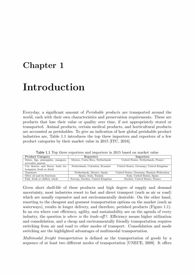
Everyday, a significant amount of Perishable products are transported around theworld, each with their own characteristics and preservation requirements. These areproducts that lose their value or quality over time, if not appropriately stored ortransported. Animal products, certain medical products, and horticultural productsare accounted as perishables. To give an indication of how global perishable productindustries are, Table 1.1 introduces the top three importers and exporters of a fewproduct categories by their market value in 2015 [ITC, 2016].
Table 1.1 Top three exporters and importers in 2015 based on market valueProduct Category Exporters ImportersDates, figs, pineapples, mangoes,avocados, guavas
Mexico, Costa Rica, Netherlands United States, Netherlands, France
Cut flowers and flower buds forbouquets, fresh or dried
Netherlands, Colombia, Ecuador United States, Germany, United Kingdom
Tomatoes Netherlands, Mexico, Spain United States, Germany, Russian FederationOlive oil and its fractions Spain, Italy, Tunisia Italy, United States, SpainFish, fresh or chilled, whole Norway, Sweden, United Kingdom Sweden, United States, France
Given short shelf-life of these products and high degree of supply and demanduncertainty, most industries resort to fast and direct transport (such as air or road)which are usually expensive and not environmentally desirable. On the other hand,resorting to the cheapest and greenest transportation options on the market (such aswaterways), results in longer delivery, and therefore, perished products (Figure 1.1).In an era where cost efficiency, agility, and sustainability are on the agenda of everyindustry, the question is where is the trade-off?. Efficiency means higher utilizationand consolidation, and a cheap and environmentally friendly transportation requiresswitching from air and road to other modes of transport. Consolidation and modeswitching are the highlighted advantages of multimodal transportation.
Multimodal freight transportation is defined as the transportation of goods by asequence of at least two different modes of transportation [UNECE, 2009]. It offers

4 Chapter 1. Introduction
Figure 1.1 The paradox of planning transportation of perishable products
a potential platform for a more efficient, reliable, flexible, and sustainable freighttransportation. However, planning operations of a multimodal system, added to theextra product preservation of perishable products, is heavily complex. The currentthesis addresses this complexity, motivated by a real-world transportation system.
1.1 Motivation and Challenges
The current thesis was inspired by the Europe-wide transportation of horticulturalproducts, sold in the Dutch markets. Horticultural industry is a branch of agriculturalindustry, where companies are involved in cultivation, process, trade, logistics, andsale of plant products. Examples of horticultural products are plants, flowers, fruits,vegetables, nuts, seeds, herbs, mushrooms, medicinal plants, and non-food crops suchas grass and ornamental trees.
The Dutch horticultural industry is globally well-recognized by the leading role itplays internationally. It is the largest exporter of fresh products in Europe and oneof the top three largest exporters in the world. Everyday around 400, 000 types offlowers and plants are sold in six auction locations around the Netherlands as wellas online, with average turnover of more than 8 million Euros per day [FloraHolland,2015]. Kenya, Ethiopia, Israel, Netherlands, Belgium, Germany are among the topproducers of these products, and United Kingdom, Netherlands, Germany, France,Italy, Poland, and Russia are among the top European markets.
Nowadays, most horticultural products are transported from the growers to auctionhouses, inspected, auctioned, and delivered to the buyers and customers on regularroutines and on fixed routes (Figure 1.2). The foreign products are mainly transportedto the Netherlands by airplanes, and almost the entire long-haul transportation ofproducts throughout Europe is done by trucks. It is estimated that almost one outof ten trucks on Dutch roads is filled with flowers and plants, and this number isexpected to increase [DAVINC3I, 2011].
So far, the Dutch horticultural industry has been successful and efficient in tradition-

1.1 Motivation and Challenges 5
Figure 1.2 An illustration of the current supply chain (extended from EVO [2009])
ally managing its transportation. However, similar to other industries, it is facingnew trends forcing its leaders to adapt and innovate. These trends and their resultingtransportation issues are [DAVINC3I, 2011]:
� New markets in developing countries (in Eastern Europe) are rising and newproduction sites (in Africa, South America, and East Asia) are joining thehorticultural chain. This is translated into a significant change of network flowvolume on both sides of supply and demand.
� E-commerce advances are changing the traditional way of trade, pushing theindustry to virtualize its business. This means decoupling information andfinancial flows from the physical one, which again changes the transportationnetwork. In the traditional scenario, products are transported in and out ofauctioning locations, but on a virtualized platform, products can directly betransported from their suppliers to the final customers.
� New cold-chain technologies are being developed to improve product preserva-tion process and therefore product quality. Such advances would facilitate longertransportation and handling, which furthermore lifts hard time constraints, andwelcomes more transportation options into the picture.
� The transportation network itself is evolving. Construction of new traintracks and waterways around Europe, establishment of new intermodal hubsand cross-docks, and relaxation of international custom regulations, are some

6 Chapter 1. Introduction
Figure 1.3 Average sale percentage of flowers to the main European markets for eachday of week
of the examples. These changes should also be incorporated in an efficienttransportation plan.
� New environmental regulations and taxes are being enforced that oblige theindustry to look for greener logistics and transportation, which the traditionaltruck-only transportation might not be able to achieve. This would requiretailored planning models and algorithms for a multimodal transportationplatform.
The sector wants to strengthen its global leading position, and providing value-added logistics services is one of their strategies. To be more specific, the sectoris aiming to lower related logistics costs in 2020 by 15%, equivalent to 64 millionEuroes [FloraHolland, 2015].
Challenges
An optimal transportation plan of perishable products needs to deal with severalchallenges. Weather unpredictability, labour costs, and political issues have a directinfluence on the production, which makes the supply uncertain. At the other end ofthe chain, economic power of household, cultural and political changes, and ceremonialoccasions, can significantly cause the demand to fluctuate. Therefore, the volume andfrequency of products to be transported are highly dynamic and uncertain. Figures1.3 and 1.4 show just how the average daily and weekly demand for flowers vary in theDutch horticultural industry [Tosi, 2014, Verhoeven, 2014, Vlassak, 2014, Rosenboom,2014].
Supply and demand dynamics are added to the operational challenges such as 1)controlling and preserving product quality, 2) taking the conditions and limitations

1.1 Motivation and Challenges 7
Figure 1.4 Average sale percentage of flowers for each week of 2013
of the available transportation network into account, and 3) managing the resources.Some horticultural products are highly perishable, losing 15% of their value per day.Recent RFID1, sensor, and information technology advances, along with agriculturalengineering developments have eased the first challenge, easing the shift from truck-only to more multimodal long-haul transportation. However, there is not muchknowledge on what a multimodal transportation of perishable products would looklike, which modes could be used for transporting them, and how much it would cost.
Whilst drawing a multimodal transportation, management of logistics resources yetstays challenging. Resources can be empty loading units, vehicles, crews, powerunits, engines, etc. Positioning, balancing, repositioning, and rotation of theseresources are the subject of resource management. In the Dutch horticultural industry,management of empty loading units, called Returnable Transport Items (RTIs), isdelicate. RTIs can have different sizes ranging from a small box to a large 45-feetcontainer. In the Dutch horticultural industry, flowers and bouquets are transportedin small RTIs (e.g. boxes or buckets) and plants in medium ones (e.g. cages ortrolleys). Their number in the entire chain is limited, and their shortage at locationswhere they are needed results in quality decay of the products waiting for them, whichtherefore results in lost sales and less profit. These RTIs are owned by the cooperativeparty, stored mainly in two auction locations, and are leased to growers, exporters,and transportation companies. These companies are then expected to return RTIsback to their storage locations in time. Returning or repositioning these units is costlyand does not bring any direct profit.
According to the review paper by Ahumada and Villalobos [2009] on planningapproaches for perishable product supply chains, there is an evident gap in theliterature on transportation planning of these products considering the dynamics,uncertainty, and risks involved. The main contribution of this thesis is then to fill
1Radio-Frequency IDentification (RFID)

8 Chapter 1. Introduction
the gap within its own scope, which is multimodal long-haul transportation planning,including management of the crucial resources.
1.2 Perishability in Transportation Planning Liter-ature
In order to be able to frame the problems addressed in this thesis, outline theobjectives, and clarify its contributions, this section gives an overview on the literatureof planning transportation of perishable products.
This literature is distinguished by extra preservation constraints or penalty costs. Ta-ble 1.2 provides an overview of the literature on transportation of perishable products,grouped into long-haul transportation, and last-mile (or first-mile) transportation.
Last-mile distribution is the transportation of products from a central hub, which isusually a warehouse or a distribution center, to the final shops or customers. First-mile on the other hand is the transportation of products from growers or factories to acentral hub, which is a consolidation or a logistics service center. Traditionally, theseparts of transportation cover small geographic areas and are carried out by truck-onlyoptions, but are not definite. Long-haul transportation in contrast is the one amonghubs dispersed around the network and connected by multimodal options.
Last-mile distribution of products is usually modeled as Vehicle Routing Problemswith Time Windows (VRPTW) and the goal is to find the optimal load, deliveryroutes, and departure times of vehicles. Akkerman et al. [2010] provide anoverview on the quantitative operations management approaches to food distributionmanagement, with focus on food quality, food safety, and sustainability aspects.Regarding quality preservation modeling, they conclude that including temperaturebased control technologies and models, is very limited in the literature and calls forfurther research. Doerner et al. [2008] study the pickup problem of blood productswith strict interdependent time windows. They model it as a Mixed-Integer Program(MIP), and present a branch-and-bound and three heuristic algorithms to solve it.Their objective is to minimize the time that vehicles travel to collect all the products.Hsu et al. [2007] model a food distribution planning problem with stochastic andtime-dependent travel times and time-varying temperature. Their objective is to finda trade-off between transportation and inventory costs, while minimizing the lossof served foods to customers. They propose a MIP and a Time-Oriented Nearest-Neighbor Heuristic to solve it. Osvald and Stirn [2008] address distribution of freshvegetables with time-dependent travel times, but add a quality degradation based costfunction to the objective function. They model this problem and use a simple heuristicto solve it for a real-world case. Tarantilis and Kiranoudis [2001] and Tarantilis andKiranoudis [2002] study the distribution of fresh dairy with a heterogeneous fixed fleet,and the distribution of fresh meat in a multi-depot network, respectively. However,

1.2 Perishability in Transportation Planning Literature 9
Tab
le1.2
Rec
ent
OR
lite
ratu
reon
transp
ort
ati
on
pla
nnin
gpro
ble
ms
wit
hp
eris
hable
pro
duct
s
Refe
rence
Product
Proble
mC
ate
gory
Transp
orta
tion
Mode
Transp
orta
tion
Rela
ted
Featu
res
Doerner
et
al.
[2008]
Blo
od
Fir
st-m
ile
Tru
ckin
terd
epen
den
tT
W
Apaia
hand
Hendrix
[2005]
Pea
-base
dP
rote
inP
rod
uct
ion
-Dis
trib
uti
on
Tru
ck,
Tra
in,
Barg
e,S
hip
-
Ahum
ada
and
Villa
lob
os
[2011]
Tom
ato
an
dp
epp
erP
rod
uct
ion
-Dis
trib
uti
on
Tru
ck,
Tra
in,
Pla
ne
choic
eof
mod
ep
ercr
op
Gig
ler
et
al.
[2002]
-S
up
ply
Ch
ain
Des
ign
--
Borto
lini
et
al.
[2016]
Ap
ple
,O
ran
ge,
Pea
r,P
ota
to,
Tom
ato
,B
russ
elsp
rou
tL
on
g-h
au
lT
ruck
,T
rain
,P
lan
ech
oic
eof
mod
ep
ercr
op
Reis
and
Leal
[2015]
Soyb
ean
Lon
g-h
au
lT
ruck
,T
rain
choic
eof
mod
e
Derig
set
al.
[2011]
Food
an
dp
etro
lL
ast
-mil
eT
ruck
flex
ible
com
part
men
tsin
tru
cks
Hsu
et
al.
[2007]
Food
Last
-mil
eT
ruck
dyn
am
icte
mp
eratu
re,
stoch
ast
ictr
avel
tim
e
Hu
et
al.
[2009]
Food
Last
-mil
eT
ruck
-
Mendoza
et
al.
[2011]
Mu
ltip
leP
rod
uct
sL
ast
-mil
eT
ruck
stoch
ast
icd
eman
ds,
fixed
com
part
men
tsin
tru
cks
Osv
ald
and
Sti
rn
[2008]
Veg
etab
les
Last
-mil
eT
ruck
dyn
am
ictr
avel
tim
es
Taranti
lis
and
Kir
anoudis
[2001]
Dair
yL
ast
-mil
eT
ruck
-
Taranti
lis
and
Kir
anoudis
[2002]
Mea
tL
ast
-mil
eT
ruck
-
Refe
rence
Proble
mT
yp
eQ
uality
Const
rain
tsP
rop
ose
dSolu
tion
Alg
orit
hm
Ob
jecti
ve
Doerner
et
al.
[2008]
VR
PT
Wex
pir
ati
on
TW
ab
ran
ch-a
nd
-bou
nd
,th
ree
heu
rist
ics
(min
)to
tal
dri
vin
gti
me
Apaia
hand
Hendrix
[2005]
LP
-a
tim
e-ori
ente
dn
eare
st-n
eighb
or
heu
rist
ic(m
in)
tota
lp
rod
uct
ion
an
dtr
an
sport
ati
on
cost
s
Ahum
ada
and
Villa
lob
os
[2011]
LP
mod
e-d
epen
den
td
ecay
esti
mati
on
-(m
ax)
tota
lex
pec
ted
(rev
enu
e-q
uali
tylo
ssp
enalt
ies)
Gig
ler
et
al.
[2002]
DP
qu
ali
tyst
ate
base
don
ap
pea
ran
cean
dti
me
-(m
in)
tota
lch
ain
cost
s
Borto
lini
et
al.
[2016]
LP
travel
tim
e-
(min
)to
tal
op
erati
ng
cost
,ca
rbon
footp
rint,
an
dd
eliv
ery
tim
e
Reis
and
Leal
[2015]
LP
esti
mate
dp
rod
uct
loss
per
gro
wer
-(m
ax)
tota
lm
arg
inal
pro
fit
Derig
set
al.
[2011]
VR
P-
sever
al
met
ah
euri
stic
s(m
in)
tota
ltr
an
sport
ati
on
cost
s
Hsu
et
al.
[2007]
VR
PT
Wlo
ssof
food
-(m
in)
tota
lco
sts
Hu
et
al.
[2009]
VR
P-
IP-b
ase
dm
etah
euri
stic
(min
)to
tal
tran
sport
ati
on
cost
s
Mendoza
et
al.
[2011]
VR
P-
thre
est
och
ast
icp
rogra
mm
ing
heu
rist
ics
(min
)to
tal
tran
sport
ati
on
cost
s
Osv
ald
and
Sti
rn
[2008]
VR
PT
Wlo
ad×
tim
ea
heu
rist
ic(m
in)
tota
l(t
ran
sport
ati
on
+qu
ali
tylo
ssp
enalt
ies)
Taranti
lis
and
Kir
anoudis
[2001]
VR
P-H
FF
-B
AT
A(m
in)
tota
ltr
an
sport
ati
on
cost
s
Taranti
lis
and
Kir
anoudis
[2002]
VR
P-
LB
TA
(min
)to
tal
tran
sport
ati
on
cost
s
1V
RP
:V
ehic
leR
ou
tin
gP
rob
lem
,T
W:
Tim
eW
ind
ow
s,IP
:In
teger
Pro
gra
m,
LP
:L
inea
rP
rogra
m,
DP
:D
yn
am
icP
rogra
m,
HF
F:
Het
erogen
eou
sF
ixed
Fle
et2
BA
TA
:B
ack
track
ing
Ad
ap
tive
Th
resh
old
Acc
epti
ng
alg
ori
thm
,L
BT
A:
Lis
t-B
ase
dT
hre
shold
Acc
epti
ng
alg
ori
thm

10 Chapter 1. Introduction
neither of them exclusively contemplate the perishability of products. Tarantilis andKiranoudis [2001] propose a Backtracking Adaptive Threshold Accepting (BATA)algorithm, and Tarantilis and Kiranoudis [2002] use a List-Based Threshold Accepting(LBTA) algorithm to solve their real-world cases.
In addition to the perishability, in some distribution systems, the products areincompatible and they cannot be loaded in the same truck or unit. Planning forsuch products separately, and allocating separate trucks, while customers order themsimultaneously, results in excessive transportation costs. One solution is to divide thetruck space into compartments and load each compartment with a unique producttype. The examples in the literature are Derigs et al. [2011] and Mendoza et al. [2011].Derigs et al. [2011] study such a distribution planning problem for food and petrol,where the products are incompatible and they should be separated. They model it asa VRP with flexible compartments and propose several metaheuristics to solve thisproblem. Mendoza et al. [2011] study another VRP with compartment and stochasticdemand, and design three heuristics based on stochastic programming, and comparetheir performance.
Supply chain design and production-distribution types of problem in the literaturealso study transportation planning implicitly. Apaiah and Hendrix [2005] design asupply chain for pea-based protein food with production, preparation, and processinglocations. They present a Linear Program (LP) for this production-transportationproblem, where products can be transported by multiple transportation modes.Ahumada and Villalobos [2011] present a model for planning integrated productionand distribution of fresh products. Their MIP includes maximizing the profit whileconsidering all production costs and costs of transportation by multiple modes anda quality decay penalty which is estimated based on mode type. Both Apaiah andHendrix [2005] and Ahumada and Villalobos [2011] assume to have multiple modesof transportation between pairs of location on different chain layers, but in the latter,they explicitly choose the optimal transport mode for each location pair. From adifferent perspective, to design a supply network for agri chains, Gigler et al. [2002]use Dynamic Programming (DP) methods to explicitly deal with the appearanceand quality of products over the operations. Appearance states are influenced byhandling actions. Quality states are influenced by processing, transportation andstorage actions.
The research work found in the literature that explicitly studies long-haul trans-portation is very limited. Reis and Leal [2015] propose a MIP model for a soybeanshipping chain planning problem where choice of transportation mode is includedin the model besides decisions for annual crop purchase. Since their real-worldapplication deals with significant uncertainty related to crop production, they defineseveral combinations of scenarios for this uncertainty and apply their MIP modelto each scenario in order to give insights to their decision makers. Bortolini et al.[2016] propose a tri-objective LP for tactical planning of a food distribution networkconsidering operating cost, carbon footprint and delivery time goals. They apply their

1.3 Transportation Planning Problems and Scope of Thesis 11
tool to a real-world distribution case and show the trade-off between the operationalcosts and the carbon footprint.
Reis and Leal [2015] and Bortolini et al. [2016] published their papers during thedevelopment of the current thesis, which shows studying long-haul transportation ofperishable products is gaining more attention. The framework of this thesis and itsscope are different from Reis and Leal [2015] and Bortolini et al. [2016], and its maincontribution is to include management of RTIs into the planning.
1.3 Transportation Planning Problems and Scopeof Thesis
So far, the motivation, challenges, and the methods used for dealing with productquality preservation in the literature of transportation planning, were pointed out.For framing the scope and objective of the thesis, this section takes a look at differentplanning problems that arise in transporting perishable products.
From establishing a multimodal transportation until monitoring its hourly perfor-mance, there are three levels of planning problems [Crainic and Laporte, 1997,Rushton et al., 2014]. Each level has its own decisions, scope, and objectives, andinvolves certain business parties.
� Strategic planning relates to investment decisions on the present or potentialinfrastructures (networks) and assets. Examples are constructing a newrailway, expanding an existing intermodal facility, or introducing a new productpreservation technology to the industry. Strategic decisions are made based onpartial information and estimation, require underlying study, and have long-term impact.
� Tactical planning deals with utilizing the given infrastructure by choosingservices and associated transportation modes, allocating their capacities, andplanning their itineraries and frequency. Tactical decisions are made based onhistorically collected data and forecasts, but they are updated for instance everyseason or annually.
� Operational planning still looks for the best choice of transportation modes,best itineraries, and allocation of resources, but it needs to answer to theday-to-day requirements of all multimodal operators, carriers and shippers.Operational decisions deal with a dynamicity and stochasticity that is notexplicitly addressed at strategic and tactical levels. If the pace of dynamicity ishigh, and the frequency of planning becomes real-time, operational planning iscalled real-time or online planning.

12 Chapter 1. Introduction
Figure 1.5 Scope of this thesis as highlighted
Scope of Thesis
In the scope of this thesis, it is assumed that a multimodal infrastructure and properquality control and preservation technologies are present and ready to use. Thereasons are threefold:
1. any network expansion or change is in domain of governmental and nationalorganizations and a perishable product industry is merely a user of such anetwork,
2. there is no profit in owning vessels, trains, etc., when a perishable productindustry is not able to use them with high frequency and capacity utilization,
3. advancing quality control and preservation technologies is in the area ofchemical, biological, and electrical engineering.
Therefore, strategic planning is out of scope, and the content of this thesis is dividedinto two parts, dedicated to studying tactical and operational planning (Figure 1.5).
1.4 Research Objectives
For each planning part, the related problems should be defined, modeled, andoptimized, to be able to obtain efficient plans. The research objectives of this thesisare formulated in this respect.

1.4 Research Objectives 13
Tactical Planning
The first step to plan multimodal transportation for perishable products is tounderstand its dynamics, the decisions to be made, the factors influencing them,and the objectives. The next step is to translate these elements into measurablevariables and tangible relations. Therefore, the first research objective is:
Research Objective 1: Model the multimodal transportation planning problem andpropose a mathematical formulation to optimize it.
In modeling the multimodal transportation planning with perishable products andmanagement of RTIs, measuring and preserving the product quality should be ad-dressed. In addition, characteristics of different transportation modes, regarding theirschedules, capacity, etc. should be contemplated. Finally, the flow, repositioning, andbalance of the RTIs used for transporting the products should be included.
The dimensions and complexity of this tactical planning problem confine its abilityto find solutions for the real-world cases, therefore, the second research objective is:
Research Objective 2: Develop an algorithm for multimodal transportation plan-ning and resource management of perishable products.
This algorithm should provide good solutions within reasonable computational time,considering all constraints and requirements of the planning problem modeled above.
Operational Planning
Tactical planning models and decision tools alone are not sufficient for the day-to-daymanagement of operations. A transportation system is constantly changing from oneday to the next, and the dynamics of these changes require different decisions to bemade, more detailed factors to include, and probably different objectives to consider.Therefore, a new platform is needed to optimize the day-to-day operations. In thisregard, the first objective is:
Research Objective 3: Develop a framework for operational planning of multimodaltransportation with perishable products and management of RTIs.
This framework should take the day-to-day changes of the system into account, andbased on the information it receives and its observation of the system evolution,provides efficient actions and adjustments.
Relying on available information, representing what demand has already been revealedand what has already happened in the system, might not provide smart and optimaltransportation solutions. Efficiency of a multimodal transportation depends heavilyon consolidation. The developed framework does not have any view on future, whilehaving an anticipation of what comes next, might help finding better consolidation,and therefore, more efficiency. In perishable industries, demand for transporting

14 Chapter 1. Introduction
Figure 1.6 Perishable transportation planning as explored in this thesis
products is dynamic and uncertain, and there are various trends (e.g daily, weekly,and seasonal) causing it to fluctuate. Therefore, the next objective is:
Research Objective 4: Model anticipation of future demand and incorporate it inthe developed operational planning framework.
Even though future demand is uncertain, there is historical data available on itsbehavior. Based on the insights that this data provides about future demandscenarios, the modified framework should take different actions, offering a smarterand more flexible transportation.
1.5 Outline of Thesis and its Contribution
In this thesis, relevant models and algorithms for tactical and operational planning ofmultimodal transportation of perishable product are developed. Figure 1.6 illustratesthe structure of this thesis based on the research objectives described earlier. Thecontent of this thesis can be divided into two groups of tactical subjects (Part II) andoperational subjects (Part III).
Section 1.2 provided an overview and the place of this thesis in the literature ofplanning the transportation of perishable products. In order to position the currentthesis in the literature of multimodal transportation planning, first in Chapter 2,an overview of the recent research on tactical and operational planning problems

1.5 Outline of Thesis and its Contribution 15
of multimodal freight transportation is presented. This chapter highlights recentmodeling and algorithm design advances, and identifies some gaps that can be subjectsof future work. Taking these gaps into account, this thesis contributes to the literaturefrom the perspective of perishable product transportation, including management ofthe crucial resources.
As part of the tactical planning, in Chapter 3, the planning problem of multimodaltransportation of perishable products, with its decisions and constraints regardingthe flow of products, the repositioning of RTIs, and arrangement of multimodal fleet,is described. Then, a MIP is proposed for it, which is an extension of the Fixed-costCapacitated Multicommodity Network Flow Problems (FCMNFP). The contributionof this chapter is in adding new sets of constraints to the classic FCMNFP. Theseconstraints include a product quality measure based on temperature and travel time,and enforces a maximum limit on products after which they are considered perished.Moreover, the forward flow of loaded RTIs is integrated with the backward flow ofempty ones via a set of novel constraints. Based on RTI demands, these constraintsautomatically assign and move the needed empty ones. Due to severe complexity ofthis problem, in this thesis only one size of RTI (e.g. cages, Dense fusters, staplewagons, trolleys) is studied. Detailed computational results and analysis are alsopresented in this chapter. Appendix A later extends this single-RTI planningproblem to include three sizes of RTIs, where RTIs of each size should be loaded(or nested) into its immediate bigger size in order to be transported. In practice forinstance, buckets and boxes are loaded onto trolleys, and trolleys later are loadedinto containers. Compared to a state-of-the-art heterogeneous resource managementproblem, this problem has extra complexity due to the loading nesting relations ofRTIs. The extended MIP for this problem is also computationally tested and verified.
In Chapter 4, a solution algorithm is proposed to solve the MIP of Chapter 3.The proposed algorithm is an adaptation of the classic Adaptive Large NeighborhoodSearch (ALNS) algorithm. Application of ALNS algorithms is new to the FCMNFPliterature, and the contribution of this chapter is in the design of new neighborhoods,and in the introduction of extra search strategies to improve performance of thealgorithm. Later in this chapter, comprehensive computational analysis on theproperties of the algorithm is presented.
In the operational planning part, in Chapter 5, first the operational planningproblem of long-haul transportation of perishable products, with its decisions andconstraints is described. This problem is a dynamic extension to the planning problemof Chapter 3. Then, a rolling-horizon framework is proposed, where based on collecteddata on the arrived demand and system evolution, a deterministic FCMNFP isperiodically solved to provide new and adjusted plans, in order to efficiently respondto the new demand and system changes. A modified ALNS is embedded in theframework to solve its FCMNFP problem. This is the first time a rolling horizonapproach is designed for operational planning of the multimodal transportation forperishable products and with repositioning of empty RTIs. Another contribution of

16 Chapter 1. Introduction
this chapter is in studying the role of different updating policies in the framework.Likewise, detailed computational analysis on the properties of the framework, alongwith some practical insights, is provided.
The framework of Chapter 5 does not include any anticipation of future demand.Therefore, in Chapter 6, this rolling horizon framework is further extended to includea stochastic FCMNF modeled as a Scenario-based Two-stage Stochastic Program(STSP), where a set of scenarios is generated and a redesigned ALNS algorithm isemployed to solve this scenario-based problem. The main contributions of this chapterare in the STSP model and the ALNS algorithm with its new operators. Anothercontribution of this chapter is in investigating the scenario generating strategiesand their influence on efficiency of solution quality and computational time. Adetailed computational analysis is presented on the scenario generation, and the roleof anticipation.
Finally, in Chapter 7, some remarks and conclusions are presented, and some futureresearch suggestions are given.
The content of this thesis is based on the following papers:
� SteadieSeifi M., Dellaert N., Nuijten W., van Woensel T., and Raoufi R.(2014), “Multimodal Freight Transportation Planning: A Literature Review”,European Journal of Operational Research 223 (1), 1–15.
� SteadieSeifi M., Dellaert N., Nuijten W., and van Woensel T.(2016), “Ametaheuristic for the multimodal network flow problem with product qualitypreservation and empty repositioning”, submitted to Transportation ResearchPart B: Methodological.
� SteadieSeifi M., Dellaert N., and van Woensel T. (2017), “A rolling horizonframework for operational planning of multimodal transportation with perish-able products, empty repositioning, and stochastic demand”, to be submitted.
� SteadieSeifi M., Dellaert N., and van Woensel T. (2017), “A multimodal networkflow problem with product quality preservation and multi-size reusable transportunits”, BETA working paper 522.

Chapter 2
Multimodal FreightTransportation: A LiteratureReview on Tactical andOperational Planning
In Section 1.2, this thesis was placed in the literature of transportation planningof perishable products. It was shown that the research on long-haul transportationof these products, and explicitly modeling temperature-based quality measures, islimited. This thesis is aiming to contribute to that literature by studying themultimodal transportation of these products. Multimodal transportation offersan advanced platform for more efficient, reliable, flexible, and sustainable freighttransportation. In order to define the contribution of this thesis in the literatureof multimodal freight transportation planning, this chapter presents a structuredoverview of the recent literature, focusing on tactical and operational planning, whererelevant models and their developed solution techniques are presented. This chapterstarts with defining the multimodal transportation and its different terminologies inSection 2.1. Then, Section 2.2 presents the recent developments on tactical planningproblems and Section 2.3 gives an overview on recent papers about operationalplanning problems. The reviewed literature in this chapter were approached bylooking at their motivations, characteristics of the different encountered problems,and their respective solution methods. These sections then were built around more orless the same structure: (1) a description of the conceptual and mathematical models(2) the solution methods used and (3) the opportunities for future research based onthe identified gaps. Finally, overall conclusions and some future research is providedin Section 2.4.
18 Chapter 2. Multimodal Freight Transportation: A Literature Review
2.1 Multimodal Transportation
Freight transportation is a key supply chain component to ensure the efficientmovement and timely availability of raw materials and finished products [Crainic,2003]. Demand for freight transportation results from producers and consumerswho are geographically apart from each other. Following trade globalization, theconventional road mode is no longer an all-time feasible solution, necessitating othermeans of transportation (and their combinations). In this regard, in 2010 about 45.8%of total freight transportation in European union countries were transported via road,36.9% via sea, around 10.2% via rail, and 3.8% via inland waterways [EUROSTAT,2012].
The freight transportation market has witnessed several trends. In many parts of theworld, new markets are rising and the customer base is growing. Furthermore, severaltrade regulations encourage easier and smoother international trade. Following theeconomic crisis in 2008, many industries browsed their business processes in order todecrease their costs and increase performance. As a consequence, shippers, carriers,and Logistics Service Providers (LSP) were urged to work at lower cost, while stillmaintaining high quality. Companies saw the solution in more cooperation andintegration, as such utilizing resources more efficiently.
Besides economic factors, environmental concerns are high on the agenda. Newregulations and taxes were raised to encourage companies to shift to more sustainablesolutions. Clearly, in this context, efficient and effective transportation is needed, asthe transportation cost share in the supply chain is significant [Ghiani et al., 2013].
A transportation chain is basically partitioned in three segments: pre-haul (or firstmile for the pickup process), long-haul (door-to-door transit of containers), and end-haul (or last mile for the delivery process). In most cases, the pre-haul and end-haul transportation is carried out via road, but for the long-haul transportation,road, rail, air and water modes can be considered. As pointed out, long-haultransportation usually involves combining different modes, but also in pre- andend-haul transportation, more and more multimodal systems are observed (usinga combination of trucks and bicycles in city logistics, for instance).
All literature discussed in this chapter focuses on multimodal freight transportation,most of which is containerized (growing around 15% annually). Key reasons forcontainerization are an increase in the safety of cargo, reduction of handling costs,standardization, and accessibility to multiple modes of transportation [Crainic andKim, 2007].
The research in the area of multimodal transportation planning accelerated duringthe last decade. The chapters of Crainic [2003] and Crainic and Kim [2007] onlong-haul and intermodal transportation, the review papers of Bontekoning et al.[2004], Macharis and Bontekoning [2004], Christiansen et al. [2007] and Bektas andCrainic [2007] are the most notable review papers on multimodal transportation

2.1 Multimodal Transportation 19
planning problems. This chapter investigates the recent research on long-haulfreight transportation planning. Public transportation, the ‘pure’ pre-haul and end-haul transportation problems and city distribution planning are out of scope. Theinterested reader is referred to Laporte [2009] for an overview on vehicle routingsolution developments and PDH for a review on pickup and delivery problems. Tokeep the length of this chapter reasonable, the operational planning of multimodalterminals is also out of scope. The review paper by Stahlbock and Voß [2008] gives anice overview in this field. Furthermore, the state of the practice is not reviewed here.Gorman et al. [2014] explore the state of the practice of Operations Research (OR)in freight transportation, and highlight recent successfully used analytical techniquesin oceanic transportation and port operations, and barge, freight rail, intermodal,truckload, less than truckload, and air freight transportation, as well as the use ofOR techniques in third-party logistics.
Over the years, different terminologies circulate in the literature and in the industry:multimodal, intermodal, co-modal, and more recently, synchromodal transportation.
Multimodal transportation: Multimodal freight transportation is defined as thetransportation of goods by a sequence of at least two different modes of transportation[UNECE, 2009]. The unit of transportation can be a box, a container, a swap body,a road/rail vehicle, or a vessel. As such, the regular and express delivery system ona regional or national scale, and long-distance pickup and delivery services are alsoexamples of multimodal transportation.
Intermodal transportation: Intermodal freight transportation is defined as aparticular type of multimodal transportation where the load is transported from anorigin to a destination in one and the same intermodal transportation unit (e.g. aTEU1 container) without handling of the goods themselves when changing modes[Crainic and Kim, 2007]. Intermodal terminals around the globe give companies theflexibility and the economies of scale of using multiple modes.
Co-modal transportation: This type of transportation focuses on the efficient useof different modes on their own and in combination. Co-modality is defined by theCommission of the European Communities [CEC, 2006] as the use of two or moremodes of transportation, but with two particular differences from multimodality: i)it is used by a group or consortium of shippers in the chain, and ii) transportationmodes are used in a smarter way to maximize the benefits of all modes, in terms ofoverall sustainability [Verweij, 2011].
Synchromodal transportation: Synchromodal freight transportation is positionedas the next step after intermodal and co-modal transportation, and involves astructured, efficient and synchronized combination of two or more transportationmodes. Through synchromodal transportation, the carriers or customers selectindependently at any time the best mode based on the operational circumstancesand/or customer requirements [Verweij, 2011].
1Twenty-foot Equivalent Unit

20 Chapter 2. Multimodal Freight Transportation: A Literature Review
The comment aspect in all definitions is the use of more than one transportationmode. Of course, the devil is in the details and some definitions put more emphasison certain aspects of the transportation process. Synchromodal emphasizes the (real-time) flexibility aspect [van Riessen et al., 2015], intermodal focuses on the sameloading unit, and co-modal adds resource utilization. Note, however, that the basicdefinition of multimodal transportation does not exclude any of the other definitions.Multimodal is the broadest definition and includes the other notions. In what follows,multimodal is used consistently.
There are three levels of decision horizon for planning problems: strategic, tactical, andoperational planning. Since this thesis focuses on tactical and operational planninglevels, the interested reader is referred to SteadieSeifi et al. [2014] for an overview onstrategic planning problems.
2.2 Tactical Planning Problems
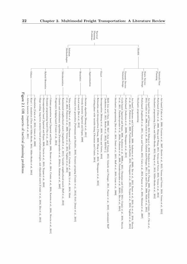
Tactical planning problems deal with optimally utilizing the given infrastructure bychoosing services and associated transportation modes, allocating their capacities toorders, and planning their itineraries and frequency. Table 2.1 and Figure 2.1 providean overview of the literature discussed on tactical planning problems.
Deciding whether to send cargo direct or through a consolidation system entails atradeoff influenced by system costs, operation times, network structure, and customerrequirements. In the literature on tactical planning problems, mostly hub-and-spokestructures are regarded. Freight on hub-and-spoke networks is transported by a singleservice, or a sequence of services where the loads are transferred from one service to thenext at intermediate terminals. A service is characterized by its origin, destination,and intermediate terminals, its transportation mode, route, and its service capacity.Likewise, a mode is characterized by its loading capacity, speed, and price. Usually,these services and modes have fixed costs.
Following Figure 2.1, there are two groups of models. The first group, Network FlowPlanning (NFP), relates to the flow planning decisions addressing the movement oforders (commodities) throughout the network. The second group, Service NetworkDesign (SND), involves the service planning decisions including all decisions onchoosing the transportation services and modes to move those commodities.
SND problems are furthermore partitioned into static and dynamic problems. Whilein both groups one determines the frequency of the service, the capacity allocation,the equipment planning, and the routing and flow of commodities, in the former it isassumed that all problem aspects are static over the time horizon, and in the latter,at least one feature (e.g. demand) varies over time. Table 2.1 shows a growing bodyof literature in SND problems compared to NFP problems. This trend indicates thatdecision makers take the fixed cost of employing services into account and look for

2.2 Tactical Planning Problems 21Tab
le2.1
Pra
ctic
al
asp
ects
of
tact
ical
pla
nnin
gpro
ble
ms
Refe
rence
Mode
Category1
FixedSchedules
Assets2
EmptyFlows
Elasticdemand
Splitdelivery
AdditionalSchedulingIssues3
Transshipment
UncertaintyIssues
DecentralizedDecisionMaking
Additionalobjectivecomponents
Chen
and
Mille
r-H
ooks
[2012]
Fd
isru
pti
on
maxim
izin
gre
sili
ence
Cohn
et
al.
[2008]
Road
,A
irF
cost
base
don
mod
al
pri
ce
Croxto
net
al.
[2007]
F
Huang
et
al.
[2011]
Fd
isru
pti
on
Hew
itt
et
al.
[2013]
F
Meng
and
Wang
[2011]
Sh
ipF
XX
Xem
pty
un
ittr
an
sport
cost
s
Meng
et
al.
[2012]
Sh
ipF
XX
dem
an
dm
axim
izin
gnet
pro
fit
Mille
r-H
ooks
et
al.
[2012]
Fd
isru
pti
on
maxim
izin
gre
sili
ence
Verm
aand
Verte
r[2
010]
Rail
FX
DD
bi-
ob
j.in
cl.
tota
lex
posu
re
Verm
aet
al.
[2012]
Rail
FX
DD
bi-
ob
j.in
cl.
tota
lex
posu
re
Anghin
olfi
et
al.
[2011]
Rail
SX
XD
DX
tran
ssh
ipm
ent
cost
sp
lus
pen
alt
yfo
rn
ot
serv
edd
eman
ds
Ayar
and
Yam
an
[2012]
Road
,S
hip
SX
DD
pen
alt
yfo
rw
ait
ing
at
term
inals
Bekta
set
al.
[2010]
Sca
paci
tyvio
lati
on
pen
alt
y
Braekers
et
al.
[2013]
Barg
eS
XM
axim
izin
gn
etp
rofi
t
Caris
et
al.
[2012]
Barg
eS
XX
Xarc
fixed
cost
s,te
rmin
al
wait
ing
cost
s,p
enalt
yfo
rem
pty
cap
aci
ty,
an
dco
op
erati
on
cost
s
Crain
icet
al.
[2006]
S
Chang
[2008]
Road
,A
ir,
Sh
ipS
XX
bi-
ob
j.:
travel
cost
;tr
avel
tim
e
Crain
icet
al.
[2014]
Sd
eman
d
Cho
et
al.
[2012]
Rail
,A
ir,
Sh
ipS
DD
bi-
ob
j.in
cl.
tota
ltr
avel
tim
es
Choum
an
and
Crain
ic[2
011]
S
Gela
reh
and
Pis
inger
[2011]
Sh
ipS
XX
Xm
axim
izin
gn
etp
rofi
t
Hsu
and
Hsi
eh
[2007]
Sh
ipS
XX
bi-
ob
j.in
cl.
fuel
cost
s,tr
an
ssh
ipm
ent
cost
san
din
ven
tory
cost
s
Lin
and
Chen
[2008]
Road
,A
irS
XX
DD
Xtr
an
ssh
ipm
ent
cost
s
Min
het
al.
[2012]
SS
X
Pazour
et
al.
[2010]
Road
,R
ail
Sb
i-le
vel
:m
in.
tim
e,m
ax.
ben
efit
Shin
tani
et
al.
[2007]
Sh
ipS
XX
Xm
axim
izin
gn
etp
rofi
t
Agarw
al
and
Ergun
[2008]
Sh
ipD
XX
maxim
izin
gn
etp
rofi
t
Anderse
nand
Chris
tianse
n[2
009]
Rail
DX
XV
TX
travel
tim
esm
axim
izin
gn
etp
rofi
t
Anderse
net
al.
[2009b]
DX
SX
Anderse
net
al.
[2009a]
Rail
DX
SX
Syn
chw
ait
ing
tim
es
Anderse
net
al.
[2011]
DX
SX
Bai
et
al.
[2012]
DX
S
Bauer
et
al.
[2010]
DX
Xem
issi
on
cost
s
Bai
et
al.
[2014]
Dd
eman
d
Choum
an
and
Crain
ic[2
014]
DX
S
Crain
icet
al.
[2016]
DX
SX
Hoff
et
al.
[2010]
Road
DX
Xd
eman
dsy
stem
cost
s,ad
hoc
cap
aci
tyin
crea
seco
st,
han
dli
ng
an
dst
ori
ng
cost
s
Liu
met
al.
[2009]
Road
DX
XX
dem
an
dsy
stem
cost
s,ad
hoc
cap
aci
tyin
crea
seco
st
Moccia
et
al.
[2011]
Road
,R
ail
DX
XF
SX
Pederse
net
al.
[2009]
Rail
DX
SX
Puett
mann
and
Sta
dtl
er
[2010]
DX
XD
Dd
eman
dX
ou
tsou
rcin
gco
sts
for
dra
yage
carr
iers
,tr
an
ssh
ipm
ent
cost
sfo
rin
term
od
al
op
erato
r
Teypaz
et
al.
[2010]
DS
X1D
Xm
axim
izin
gn
etp
rofi
t
Zhu
et
al.
[2014]
Rail
DX
MX
X
1F
:F
low
net
work
pla
nn
ing,
S:
Sta
tic
SN
Ds,
D:
Dyn
am
icS
ND
s2
S:
Sin
gle
ass
et,
M:
Mu
lti-
ass
et3
DD
:D
eliv
ery
Dea
dli
ne,
FS
:F
lexib
leS
ched
ule
s,V
T:
esti
mati
ng
Valu
eof
Tim
e,1D
:on
e-p
erio
dD
eliv
ery,
Syn
ch:
Syn
chro
niz
ati
on
22 Chapter 2. Multimodal Freight Transportation: A Literature Review
Tactica
lP
lan
nin
gP
rob
lems
Mod
els
Netw
ork
Flo
wP
lan
nin
g
Arc-b
ased
[Coh
net
al.,
2008,
Cro
xto
net
al.,
2007,
Hew
ittet
al.,
2013,
Verm
aan
dV
erter,2010,
Verm
aet
al.,
2012]
Path
-based
[Coh
net
al.,
2008,
Men
gan
dW
an
g,
2011,
Verm
aan
dV
erter,2010,
Verm
aet
al.,
2012]
Sto
chastic
pro
gra
mm
ing
[Ch
enan
dM
iller-Hooks,
2012,
Men
get
al.,
2012,
Miller-H
ooks
etal.,
2012]
Sta
ticS
ervice
Netw
ork
Desig
n
Arc-b
ased
[Ayar
an
dY
am
an
,2012,
Bek
tas
etal.,
2010,
Bra
ekers
etal.,
2013,
Ch
an
g,
2008,
Ch
ou
man
an
dC
rain
ic,2011,
Ch
oet
al.,
2012,
Cra
inic
etal.,
2006,
Garcıa
etal.,
2013,
Gela
rehan
dP
isinger,
2011,
Lin
an
dC
hen
,2008,
Min
het
al.,
2012]
Path
-based
[An
gh
inolfi
etal.,
2011,
Ayar
an
dY
am
an
,2012,
Caris
etal.,
2012,
Pazo
ur
etal.,
2010,
Sh
inta
ni
etal.,
2007]
Sto
chastic
pro
gra
mm
ing
Dyn
am
icS
ervice
Netw
ork
Desig
n
Arc-b
ased
[An
dersen
an
dC
hristia
nsen
,2009,
An
dersen
etal.,
2009b
,B
ai
etal.,
2012,
Bau
eret
al.,
2010,
Li
etal.,
2016,
Moccia
etal.,
2011,
Ped
ersenet
al.,
2009,
Pu
ettman
nan
dS
tad
tler,2010,
Th
ion
gan
eet
al.,
2015,
Tey
paz
etal.,
2010,
Yagh
ini
etal.,
2014]
Path
-based
[An
dersen
etal.,
2009b
,T
hio
ngan
eet
al.,
2015]
Cycle-b
ased
[Agarw
al
an
dE
rgu
n,
2008,
An
dersen
etal.,
2009b
,a,
2011,
Ch
ou
man
an
dC
rain
ic,2014,
Cra
inic
etal.,
2016,
Moccia
etal.,
2011,
Para
skev
op
ou
los
etal.,
2016a,
Ped
ersenet
al.,
2009,
Para
skev
op
ou
los
etal.,
2016b
,Z
hu
etal.,
2014]
Sto
chastic
pro
gra
mm
ing
[Bai
etal.,
2014,
Dem
iret
al.,
2015,
Hoff
etal.,
2010,
Liu
met
al.,
2009]
Solu
tion
Meth
od
olo
gies
Exact
B&
B[L
inan
dC
hen
,2008];
B&
C[A
yar
an
dY
am
an
,2012,
Gela
rehan
dP
isinger,
2011,
Pazo
ur
etal.,
2010];
custo
mized
B&
P[A
nd
ersenet
al.,
2011,
Hew
ittet
al.,
2013];
B&
P&
C[]
Deco
mp
ositio
n[B
ekta
set
al.,
2010,
Verm
aan
dV
erter,2010]
Rela
xatio
nan
dd
ecom
positio
n[C
han
g,
2008,
Men
get
al.,
2012,
Th
ion
gan
eet
al.,
2015]
Cu
tting-p
lan
ew
ithvaria
ble
fixin
g[C
hou
man
an
dC
rain
ic,2014]
Ap
pro
xim
atio
n
Heu
ristics
Decisio
nalg
orith
m[H
uan
get
al.,
2011]
Greed
yh
euristic
[Agarw
al
an
dE
rgu
n,
2008]
Loca
lsea
rch[B
ai
etal.,
2012]
Scen
ario
treegen
eratio
n[P
uettm
an
nan
dS
tad
tler,2010];
Scen
ario
gro
up
ing
[Cra
inic
etal.,
2014];
SA
A[D
emir
etal.,
2015]
Meta
heu
ristics
Tab
usea
rch[B
ai
etal.,
2012,
Ch
ou
man
an
dC
rain
ic,2011,
Cra
inic
etal.,
2006,
Li
etal.,
2016,
Min
het
al.,
2012,
Ped
ersenet
al.,
2009,
Verm
aet
al.,
2012,
Yagh
ini
etal.,
2014]
Ran
dom
izedn
eighb
orh
ood
search
[An
gh
inolfi
etal.,
2011];
Varia
ble
neig
hb
orh
ood
search
[Hoff
etal.,
2010]
Gen
etican
dev
olu
tion
ary
alg
orith
m[P
ara
skev
op
ou
los
etal.,
2016a,b
,S
hin
tan
iet
al.,
2007]
Pro
gressiv
eh
edgin
g-b
ased
[Cra
inic
etal.,
2014]
Hyb
ridH
euristics
Colu
mn
gen
eratio
nb
ased
[Agarw
al
an
dE
rgu
n,
2008,
Bro
uer
etal.,
2014,
Cra
inic
etal.,
2016,
Karsten
etal.,
2016,
Moccia
etal.,
2011]
Dyn
am
icp
rogra
mm
ing
based
[Ch
oet
al.,
2012]
Deco
mp
ositio
nb
ased
[Agarw
al
an
dE
rgun
,2008,
Garcıa
etal.,
2013,
Tey
paz
etal.,
2010]
Slo
pe
scalin
g,
lon
g-term
mem
ory
-based
pertu
rbatio
nstra
tegies,
an
dellip
soid
al
search
[Cra
inic
etal.,
2016,
Zhu
etal.,
2014]
Oth
ers
Sim
ula
tion
[Caris
etal.,
2012,
Liu
met
al.,
2009]
Exact
+sim
ula
tion
[Ch
enan
dM
iller-Hooks,
2012,
Miller-H
ooks
etal.,
2012]
Ad
-hoc
heu
ristic[A
ngh
inolfi
etal.,
2011]
Figure
2.1
OR
asp
ectsof
tactica
lpla
nnin
gpro
blem
s

2.2 Tactical Planning Problems 23
Figure 2.2 (a) Space-time network with three nodes and six time periods. (b) Exampleof a feasible service plan. [Andersen et al., 2009a]
cost-efficient solutions.
In both NFP and SND problems, continuous variables are used to representcommodity flows throughout the network, but in SND problems, binary variables areincluded for selection of services. The variables can be arc-based representing flow onan arc or path-based representing flow on a path (a series of arcs). SND problems arethen modeled as Fixed-cost Capacitated Multicommodity Network Design (FCMND)problems.
Dynamic SND problems have a time dimension in the CMND formulation, making ita discrete multi-period model. Therefore, the SND problem is mapped both in timeand space, and each node in the new network represents a terminal at a time period.This space-time network has the potential to accommodate many real-life propertiesof SND problems. An example is waiting or transfer operations at a terminal,represented by arcs connecting different time periods with the same locations.Another example is different transportation modes, represented by additional arcs.Such arcs can therefore accommodate different costs for terminal operations andmodal costs. For an overview on dynamic SND problems, the interested reader isreferred to Wieberneit [2008].
In addition to planning flows of commodities, routing, and scheduling of services,managing limited available resources (assets) are also integrated with SND problems.Assets can be containers, vehicles, crews, power units, engines, etc. Positioning,balancing, repositioning, and rotation of assets are the subject of asset management.Assets follow a “full-asset-utilization” policy ensuring that the composition, capacity,and other characteristics do not change over the planning horizon. Cycle-basedvariables can be used to integrate the mode or vehicle rotation over the planninghorizon into SND models. In this order, backward arcs connecting later time periodsto earlier ones are used to represent cycles and rolling horizons. Figure 2.2 gives anillustration of a space-time network with cycle-based arcs.
In NFP and SND problems, arc-based variables are mostly used (Figure 2.1), whilepath-based and cycle-based formulations, particularly in dynamic SNDs where the

24 Chapter 2. Multimodal Freight Transportation: A Literature Review
physical network is multiplied by the number of time periods, are computationallyinteresting to study. A cycle-based formulation, as soon as the cycles are enumerated,outperforms the arc-based formulation in both time and solution quality [Andersenet al., 2009b]. Andersen et al. [2009b] show that compared to the arc-basedformulation which yield an average 5% to 20% gap, the cycle-based formulationexhibit gaps from 1% to 5%. However, the drawback is that by increasing thenumber of periods in the planning horizon, the number of cycles to be generated growsexponentially and generating them needs smart enumeration algorithms. To cope withthis problem, Andersen et al. [2011] design a customized Branch-and-Price (B&P)algorithm for the problem presented Andersen et al. [2009b] and show its superiorityto the other common exact algorithms. In their proposed algorithm, they integratetwo column generation subproblems for integer cycle design and continuous flow-path variables. They also use a combination of branching strategies, a mechanism todynamically add violated strong linear relaxation cuts, and an acceleration techniquebased on depth-first search to speed up finding integer solutions. Following thesepapers, Crainic et al. [2016] propose a hybrid heuristic, combining column generation,slope scaling, and intensification and diversification heuristics, to solve SND problemswith design-balanced requirements. They compare their approach with the previousworks and show that while it generates a relative small set of all cycles, it is capableof producing high-quality solutions. Brouer et al. [2014] also propose a hybridmetaheuristic to solve the liner shipping network design problems. In their algorithm,they use column generation to avoid extensive computation, and an integer programinside the improvement heuristic, which provides the set of services to be removed andreinserted. Karsten et al. [2016] extend this work to solve a liner shipping networkdesign problem with transit time restrictions on commodities. They introduce aspecialized label setting to take these restrictions into account.
Solving NFP and SND problems due to their large set of variables is difficult. Figure2.1 presents the solution methodologies used, and clearly shows that due tocomplexity of these problems, heuristic and metaheuristic solution methods are theprime choice. Among them, Tabu Search (TS) seems to be a popular metaheuristicalgorithm [Bai et al., 2012, Chouman and Crainic, 2011, Crainic et al., 2006, Minhet al., 2012, Pedersen et al., 2009, Verma et al., 2012]. However, no paper was foundapplying approximation techniques, which is an interesting research opportunity.
In order to evaluate the performance of the proposed algorithms, good benchmark setsare needed. The majority of the research on tactical planning level address specificreal-world problems and the algorithms designed for those problems. Thus, a solidanalysis on the efficiency of different algorithms, due to the lack of general benchmarksets, is not attainable. One can only refer to the interesting results obtained by theresearchers. For instance, Bektas et al. [2010] compare arc-based and flow-baseddecomposition methods in solving small sizes of their nonlinear problem, and showthat despite the fact that the arc decomposition has a better convergence, it takesmore time compared to flow-based decomposition. In overall, both techniques handlethe nonlinearity efficiently. Recently, Brouer et al. [2013] has offered a benchmark
2.2 Tactical Planning Problems 25
suit based on liner shipping network design problems based on industrial standardand rules, and presented the first best known solutions for them.
Zhu et al. [2014] compare the performance of their hybrid algorithm with a state-of-the-art solver for small to medium sizes of a randomly generated data set. They showthat their algorithm outperforms in computational time and even solution qualitywhen instance size grows. For instance, the combination of slope scaling and long-term memory-based perturbation achieves on average 21% improvement in solutiongap in 10 hours compared to the solver. Inclusion of ellipsoidal search even improvesthe average solution gap by 2% more. For small instance, this hybrid algorithm findsthe optimal solution of 5 out of 7 instances and reaches an average gap of 0.13% forthe others.
Ayar and Yaman [2012] use a real world data set with 34 nodes and 167 services, andgenerate a random network of 66 nodes and 1200 arcs, and test them for 400 up to 1000commodities. Their first conclusion is that by increasing the number of commodities,the average optimality gap decreases. Moreover, adding valid inequalities and variablefixing strategies result in significant improvements both in time and solution quality.All their instances are solved to optimality within 6 minutes. Ayar and Yaman [2012]also investigate variable fixing based on capacity restrictions, but in overall, it doesnot bring much improvement to their previous valid inequalities and variable fixingstrategies.
The work of Pedersen et al. [2009] is one of the examples of using TS as the baseof a solution algorithm. They use the instance sets of Crainic et al. [2000] andGhamlouche et al. [2003]. In comparison to a MIP solver, their algorithm showsrobustness, and even outperforms the solver in 33 cases of the 78 instances theytested. Although the tuning of TS is dependent to the instance characteristics, ininstances with particular structures like high fixed-variable cost ratio and/or loosecapacity, TS outperforms the MIP solver. With the use of an independent multisearchstrategy, Pedersen et al. [2009] could furthermore improve the results to 2% more.However, their TS still stands as a powerful algorithm. Li et al. [2016] decompose theirSND with heterogeneous vehicles into two interdependent sub-problems of a fixed-charge capacitated multicommodity network design problem, and a vehicle assignmentproblem (VAP). They also propose a TS with cycle-based neighborhoods to solve thisproblem. Yaghini et al. [2014] in the body of a Tabu Search algorithm, propose anew cutting-plane neighborhood for solving fixed-charge capacitated multicommoditynetwork design problem, which uses different strategies to select an open arc to beclosed. The selected arcs are either arcs with maximum combined costs, or maximumvalue of unused capacity ratio multiplied by the arcs fixed costs. They show that insolving the standard instances in the literature, their neighborhood outperforms manyother methods such as cycle-based, path relinking, multilevel, and local branchingmethods.
In comparison, Paraskevopoulos et al. [2016a] propose an evolutionary algorithm forSND problems, which using principles of scatter search, iterated local search, new

26 Chapter 2. Multimodal Freight Transportation: A Literature Review
cycle-based neighborhoods, and efficient perturbation strategies, evolves a pool ofsolutions. They show that their algorithm is able to provide high quality to optimalsolutions for the standard instances in the literature. Paraskevopoulos et al. [2016b]explicitly study congestion at nodes and its related costs in SND problems. It is anonlinear integer program, and they propose a reformulation as a mixed integer secondorder cone program, and extend the evolutionary algorithm of Paraskevopoulos et al.[2016a] to provide the upper bounds. They show that their evolutionary algorithmprovides good results in really short computational time.
Adding to the aforementioned discussions, there are many other opportunities forfuture research. Overall, Table 2.1 shows that little work has been carried out onintegrating asset management in SND problems, while in multimodal transportation,especially in containerized shipment, multiple types of loading units are involved, andrepositioning their empties is costly. Furthermore, these assets require simultaneousallocation planning. As an example, crew scheduling is usually studied independently,but it also depends on the service schedules, and embedding it in SND problems isexpected to provide higher performance efficiency. In recent literature, Zhu et al.[2014] extend the conventional SND and include car classification and blocking, andtrain make-up in a railway system. Their space-time modeling includes three layersfor service, block, and car. They design a hybrid metaheuristic algorithm combiningslope scaling, long-term memory-based perturbation strategies, and ellipsoidal searchmethod, which can solve problems with up to 10 yards, 60 tracks and 3050 services. Insolving small sized instances, in case their model cannot find the optimal solution in10 hours, it reaches an average optimality gap of 0.13%. Moreover, in solving biggersizes, it outperforms a commercial solver both in time and solution quality.
Another capital aspect of multimodal transportation systems worth more considera-tion is the transshipment of loads at terminals and its effects on the performance ofthe whole system. Transshipment is usually implicit in multimodal tactical planning,though feasibility of operations, especially in the presence of fixed timetables dependson explicit study of transshipment operations and their related costs. Meng and Wang[2011] only impose a constraint on maximum berth occupancy time for each shipdeployment plan, and Anghinolfi et al. [2011] also include a restriction on maximumhandling operations for each train at a given terminal. Still, these research works donot assess any explicit costs to these operations. Gelareh and Pisinger [2011] subtracta general transshipment costs (per container at a given port) from the revenue intheir objective function. Hamzaoui and Ben-Ayed [2011] integrate transshipmentcosts into a handling cost per container, which also includes loading and unloadingcosts. Andersen and Christiansen [2009] study the issues of border crossing and embedthe handling costs in terminals into unit flow cost.
Some papers include detailed transshipment operations and their costs. Hsu andHsieh [2007], in addition to servicing costs such as ship pilotage and berth occupancy,consider cargo handling, equipment charges, and inventory costs into their costfunction. Shintani et al. [2007] have port related costs and cargo handling costs which

2.2 Tactical Planning Problems 27
are subtracted from revenue in their objective function. Hoff et al. [2010] explicitlyinclude inventory holding costs at terminals into their objective function, and Zhuet al. [2014] include restrictions on maximum track occupation of trains at terminalsand maximum number of block-building workload at each period, along with costsrelated to these operations into their model.
Transshipment becomes more critical in the presence of cut-off times and whensynchronization of the system plays an important role in on-time delivery of time-sensitive products. Andersen et al. [2009a] seem to be the only one takingsynchronization into account. They extend the work of Andersen and Christiansen[2009] by including the synchronization within the system and with the neighboringsystems. They conclude that by more collaboration and integration of transportationsystems, significant improvement in performance can be achieved. In order to havea synchronized transportation system, studying transshipment, its conditions, andcosts offers another interesting future research direction.
However, synchronization of operations might fail if uncertainty is ignored. Assumingthe planning elements such as coming demand as deterministic generates suboptimalsolutions, redundant costs and less efficiency. Among various types of uncertainfactors, stochastic demands are studied mostly, and modeled as multi-stage stochasticprograms [Bai et al., 2014, Crainic et al., 2014, Hoff et al., 2010, Lium et al., 2009,Meng et al., 2012, Puettmann and Stadtler, 2010]. Following Lium et al. [2009] whereflexibility in face of uncertain demand is dealt with adding ad-hoc capacity increaseto the model, Bai et al. [2014] incorporate vehicle rerouting as their second meansof flexibility. Despite its expensive computation, they show that their solutions offerbetter flexibility with less outsourcing, however, it highly depends on the nature ofuncertain demand. One class of widely used approaches in solving stochastic problemsis the scenario-based approaches where the uncertain factors are represented in thestochastic programs as scenarios. The most important issue in these approaches isthen how good these scenarios represent all possibilities of the uncertain factors. Thereare many strategies in the literature such as scenario grouping. Crainic et al. [2014]propose strategies to group the scenarios based on the type of decomposing them, typeof grouping, and measures specifying their similarities, and in the body of a progressivehedging-based metaheuristic, they show that the covering strategy with respect tocommodity demands produce the highest quality solutions. Stochastic demand isnot the only source of uncertainty. Andersen and Christiansen [2009] study thevariability of travel times in their service network design, but with a different modelingapproach. They add a slack variable that represents this variability, set a penalty costfor it in their objective function, and analyze the utilization of their fleet based onpositive values of this variable. Demir et al. [2015] study an intermodal transportationplanning problem with stochastic demand and travel times, and with emission-relatedcosts. Unlike most of the SND literature where planning horizons are discretized,they propose a continuous-time mixed-integer linear programming formulation for it,and apply a Sample Average Approximation (SAA) algorithm which evaluates anextensive set of scenarios in order to develop more robust transportation plans.

28 Chapter 2. Multimodal Freight Transportation: A Literature Review
Moreover, a reliable transportation network is a network that can recover from anydisruption by preventing, absorbing, or mitigating its effects. Unexpected incidentslike traffic jam, accidents, storms, hurricane, etc. can cause disruption on a link orin a terminal. In multimodal transportation planning, providing reliable but cost-efficient services is a hard task. If the designed network is flexible enough, disruptionmight be absorbed by the normal plans, but if this flexibility has not been deliberated,recovery plans are required to revive the system and keep the promised service levels.In multimodal transportation, such recovery plans usually involve service and modalchange. In the recent literature, Huang et al. [2011], Chen and Miller-Hooks [2012],and Miller-Hooks et al. [2012] take disruption and required recovery and preparednessactions into account. Huang et al. [2011] compare the forecasted delay on a distressedlink to the tolerance threshold of the next link, and if the delay crosses the threshold,a re-routing with the smallest deviation and least cost is made. Chen and Miller-Hooks [2012] define an indicator of network resilience to assess the vulnerability ofa time-definite network and make a priori investment decisions for recovery actionwith a given budget. Resilience is defined as the ability of a network to copewith disruption via its topological and operational attributes. Miller-Hooks et al.[2012] extend this work by including preparedness actions that can provide increasedrecovery capability and increased coping capacity. Chen and Miller-Hooks [2012]omitted preparedness actions in order to decompose the problem into independentdeterministic subproblems.
Huang et al. [2011] comprise forecasting decisions, propose a decision model basedon an optimization model and an improved depth-first search method. Chen andMiller-Hooks [2012] design a framework employing Benders’ decomposition, columngeneration, and Monte Carlo simulation, and Miller-Hooks et al. [2012] present aninteger L-shaped method and Monte Carlo simulation to solve this problem. Althoughall these three groups test their models on small instances, they provide interestingresults. For instance, both Chen and Miller-Hooks [2012] and Miller-Hooks et al.[2012] indicate that competing measures such as reliability and flexibility that donot consider recovery actions may underestimate the network’s ability to cope withunexpected events. In fact, a network may not be very reliable or flexible, but maybe resilient or may be reliable or flexible, but not sufficiently resilient. Moreover, themaximum resilience is obtained from taking both preparedness and recovery options,and the more the budget is spent on preparedness options, the greater the benefitswould be.
Disruptions are usually dealt with at the operational level, treated by the costly lastminute solutions. However, the impact of a disruptive event and its aftermaths onthe performance of a multimodal transportation system is dramatic and might resultin the complete failure, especially in a large-scale international scope. Reflectingreliability and resilience into the tactical planning shows great improvement in theoperations, implying that designing suitable pre-disaster and post-disaster actionsrequires further attention.

2.3 Operational Planning Problems 29
A key element in tactical transportation planning is the role of the decisionmakers. The collaboration or competition of carriers influence the service level, thesynchronization, and the system performance. In practice, an independent partymanages each hub and leg of a multimodal transportation network. In the presence oftheir cooperation, for instance, a terminal operating company receives the informationon the arrival of a ship or trains early enough to plan the necessary unloading,transshipment and loading tasks. In addition, the cooperating carriers can reactto disruptions faster, using vehicles, modes, and resources of each other. Puettmannand Stadtler [2010] test the idea that collaboration reduces the operational costs ona chain with one multimodal operator and two carriers responsible for pre-haul andend-haul drayage. In their scheme, the three parties do not exchange any informationand plan their own operations, however they iteratively exchange proposals and theircost effects are compared to the solution without coordination. Due to the time lagbetween the departure and arrival of orders, they include stochastic demand in theirscheme, which calls for adaptation of plans. The authors present three models forthe proposal generation for the involved parties and use a scenario tree generationto quantify the expected gain of coordination. At the end, they conclude thattransportation parties can significantly reduce in operational costs by collaboration.
From a different point of view and motivated by a Belgian barge transportationnetwork, Caris et al. [2012] study a SND problem focusing on cooperation of inlandterminals and line bundling. They define different cooperation scenarios and analyzethem by means of simulation. The authors conclude that given the current transportvolumes, more bundling opportunities may be created by reducing the number ofdepartures or setting up a truck collection/distribution network. However, reducingthe number of departures may lead to less service offered to customers. This can besolved by more cooperation between inland terminals to attain economies of scale andto reduce maximum waiting times for inland barges at sea terminals.
In SND problems, the individual role of the stakeholders is usually ignored and it isassumed that the whole transportation system is managed by a central party (namelymultimodal operator). While in practice, each company has its own goal and policies,and shares limited data with others. Furthermore, these companies are competingwith each other, keeping the market dynamic and vibrant. Inclusion of cooperationand competition in tactical planning problems merit more research.
Multimodal transportation service network design is in practice a complex problemwith thousands of variables and constraints. With better study of the problemstructure and design of smarter solution algorithms, it should be possible to derivemore accurate solutions in less computational time.

30 Chapter 2. Multimodal Freight Transportation: A Literature Review
Tab
le2.2
Pra
ctical
asp
ectsof
op
eratio
nal
pla
nnin
gpro
blem
s
Refe
rence
Mode
Problem Type 1
Assets 2
Transshipment
Synchronization
AdditionalSchedulingIssues
Multiobjective
UncertaintyIssues
DecentralizedDecisionMaking
Additionalobjectivecomponents
Bandeir
aet
al.
[2009]
Road
,R
ail
FM
RA
Sall
costs
related
totra
nsp
orta
tion
of
emp
tyu
nits
Chang
et
al.
[2008]
FM
RA
S
Di
Francesc
oet
al.
[2013]
Sh
ipF
MR
AS
on
e-day
earlier
sched
ulin
gd
isrup
tion
shorta
ge
costs
Erera
et
al.
[2005]
Road
,R
ail,
Sh
ipF
MR
AS
plu
su
nsch
edu
ledserv
icesrep
ositio
nin
gan
dclea
nin
gco
stsof
conta
iners
Lam
et
al.
[2007]
Sh
ipF
MR
AS
dem
an
d
Song
and
Dong
[2012]
Sh
ipF
MR
AS
Xterm
inal
an
drep
lenish
men
tco
sts
Shi
et
al.
[2014]
FM
RA
Sd
eman
dan
dcu
stom
erT
WT
opalo
glu
[2006]
FM
RA
Sd
eman
dan
dtra
vel
times
X
Topalo
glu
[2007]
FM
RA
Sd
eman
dan
dtra
vel
times
X
Topalo
glu
and
Pow
ell
[2005]
FM
RA
Sd
eman
dX
Topalo
glu
and
Pow
ell
[2006]
FM
RA
Sd
eman
d
Topalo
glu
and
Pow
ell
[2007]
FM
RA
S
Bock
[2010]
IRP
XX
Driv
er’srest
time
travel
times
Xtra
nsp
orta
tion
costs
of
ow
ned
an
dou
tsou
rced,
load
ing
an
du
nlo
ad
ing
costs,
tard
iness
costs
incu
rredd
ue
tola
ted
eliveries
an
dla
tep
icku
ps,
an
dveh
iclefi
xed
costs
van
Heesw
ijket
al.
[2016]
IRP
XX
dem
an
dem
ission
Goel
[2010]
Road
,R
ail
IRP
Xtra
vel
times
Xco
stsarisin
gif
custo
mer
dem
an
ds
can
not
be
satisfi
edin
time
(stock
ou
tco
sts)
1F
MR
A:
Fleet
Man
agem
ent
an
dR
esou
rceA
lloca
tion
,IR
P:
Itinera
ryR
e-Pla
nn
ing
2S
:S
ingle
asset,
M:
Mu
lti-asset
3T
W:
Tim
eW
ind
ow
s

2.3 Operational Planning Problems 31
Op
erati
on
al
Pla
nn
ing
Pro
ble
ms
Model
s
Fle
etM
an
agem
ent
an
dR
esou
rce
Alloca
tion
Net
work
flow
pro
ble
m[B
an
dei
raet
al.,
2009,
Ch
an
get
al.,
2008]
Tim
e-sp
ace
rep
rese
nta
tion
[Ere
raet
al.,
2005,
Di
Fra
nce
sco
etal.
,2013,
Son
gan
dD
on
g,
2012]
Ap
pro
xim
ate
dyn
am
icp
rogra
mm
ing
[Lam
etal.,
2007,
Sh
iet
al.,
2014,
Top
alo
glu
,2006,
2007,
Top
alo
glu
an
dP
ow
ell,
2005,
2006,
2007]
Itin
erary
Re-
pla
nn
ing
Tim
e-sp
ace
rep
rese
nta
tion
[Goel
,2010]
Rou
tin
gan
dsc
hed
ulin
g[B
ock
,2010,
van
Hee
swij
ket
al.,
2016]
Solu
tion
Met
hod
olo
gie
s
Exact
Ap
pro
xim
ati
on
Heu
rist
ics
Dec
om
posi
ng
reco
urs
en
etw
ork
[Sh
iet
al.,
2014]
Dec
om
posi
tion
an
dp
riori
tiza
tion
[Ban
dei
raet
al.,
2009]
Iter
ati
ve
ap
pro
xim
ati
on
[Top
alo
glu
,2007,
Top
alo
glu
an
dP
ow
ell,
2007]
Tw
o-s
tage
short
est-
path
base
d[S
on
gan
dD
on
g,
2012]
bes
tk-r
ou
tegen
erati
ng
heu
rist
ic[v
an
Hee
swij
ket
al.,
2016]
Met
ah
euri
stic
sV
ari
ab
len
eighb
orh
ood
searc
h[B
ock
,2010]
Hyb
rid
Heu
rist
ics
Bra
nch
-an
d-B
ou
nd
heu
rist
ic[C
han
get
al.,
2008]
Oth
ers
Sim
ula
tion
[Top
alo
glu
,2006]
Sim
ula
tion
+ex
act
[Goel
,2010]
Sim
ula
tion
+ap
pro
xim
ate
policy
iter
ati
on
[Lam
etal.,
2007]
Figure
2.3
OR
asp
ects
of
op
erati
onal
pla
nnin
gpro
ble
ms

32 Chapter 2. Multimodal Freight Transportation: A Literature Review
2.3 Operational Planning Problems
On operational planning level, we still look for the best choice of services andassociated transportation modes, best itineraries and allocation of resources to thedemand. However, we need to answer the real-time requirements of all multimodaloperators, carriers and shippers. Operational planning deals with dynamicity andstochasticity that are not explicitly addressed at strategic and tactical levels. Thesecharacteristics make operational planning problems remarkably complex. Hence,designing accurate and fast solution algorithms is then essential. Table 2.2 andFigure 2.3 provide a structured view of the literature addressing operational planningproblems.
These problems relate to real-time planning for orders, and reaction and adjustment toany kind of disturbance (e.g. accidents, weather changes, or equipment breakdowns).Most of these system elements vary with time and show a non-deterministic behavior.Current decisions depend on both the present information and an estimation of thefuture, and the objective is not only to minimize the costs, but also to maximizereliability of the system. Table 2.2 and Figure 2.3 review the relating little work thathas been carried out on operational planning problems.
In order to discuss the different problems, models and solution methodologies,we group the operational planning literature under two main topics: resourcemanagement and itinerary replanning. Resource Management problems deal withthe distribution of all resources throughout the network: positioning, repositioning,storing, and allocating them to customer orders. Itinerary Replanning problems arefocused on real-time optimization of schedules, modal routes, and relevant responseto operational disturbance. Resource management and itinerary replanning problemsare in practice intertwined and act as two components of a bigger operational planningproblem. In the followings, for each group, we discuss the recent developments onmodeling and solution methods.
Resource management are problems on how and when to optimally utilize the limitedavailable resources. Some examples of these resources are vehicles (e.g. planes andtrucks), trailers, rail cars, locomotives, containers, equipments, crew, power, etc. Oncea resource is allocated to an activity, it is no longer available for certain duration.Moreover, when it becomes available again, it is often at a different location where itis not needed [Crainic, 2003]. Empty loading unit repositioning and fleet managementproblems are more specific variants of resource management problems.
In empty loading unit repositioning, there is a set of empty and reusable loading unitsthat should be shipped back from the location they are emptied to the locationsthey are needed. These loading units do not directly incorporate in the profit oftransportation, but guarantee requested service level. In empty repositioning problem,future customer demand is unknown and the objective function is to minimize emptytransportation plus storage costs, stockout costs, and in some cases, substitution costs.These problems are usually modeled as NFP problems with continuous variables to

2.3 Operational Planning Problems 33
represent the movement of the loading units. In the literature, Erera et al. [2005]compare a base repositioning strategy (a current state-of-the-practice) with threealternative strategies which integrate the repositioning and routing of the containerssimultaneously. These three strategies are weekly, bounded daily, and unboundeddaily repositioning. Erera et al. [2005] compare these strategies on a network with 10ports and 900 orders and up to 1000 containers. They show that the proper timingof repositioning is more important than deciding on the number of containers to berepositioned, and unbounded daily repositioning in overall is the best strategy.
Chang et al. [2008] investigate the substitution between containers of different typesand its interchange cost reduction. Container substitution is defined as fulfillingthe requests of one type of container with another type. In their paper, street-turnand depot-direct movement are allowed; therefore, empty containers can directly betransported among customers without passing through the terminals. They show thatwith substitution, port trips can be reduced by 70% and transportation costs from4% to 47%.
Braekers et al. [2013] show that shipping lines may reduce costs by simultaneouslyplanning barge services and empty container repositioning movements instead ofplanning empty container repositioning movements in a post-optimization phase.
These abovementioned papers exclusively study empty repositioning of loading units.However, none of them takes uncertainty or disruption (at locations or on the routes)into account. Di Francesco et al. [2013] study the effect of partial or complete portdisruption in empty container repositioning in a liner shipping system. They modelit as a time-space representation and consider a set of different disruption scenarios.They also include some non-anticipativity conditions to equalize the here-and-nowdecision variables over all scenarios. Di Francesco et al. [2013] test all combinationsof a problem including 5 locations (2 hubs), a 50 period rolling horizon scheme, 2(normal and disrupted) scenarios, and 2000 customer orders. They show that in caseof a normal scenario, the optimal deterministic solutions are the best, but in case of adisruption, the multi-scenario model produces the most effective results. Di Francescoet al. [2013] show their model is able to handle 12 disruption scenarios with up to 20locations in less than one hour.
In order to solve empty repositioning problems, different heuristics have been appliedas the solution methodologies. Chang et al. [2008] test their Branch-and-Bound(B&B) heuristic on a transportation systems with 12 consignees and 8 shippers, 2local container depots and 1 container terminal, and up to 985 containers. Bandeiraet al. [2009] implement decomposition and prioritization approaches on a 4 depotcase with 4 to 8 clients. They test and analyze the performance for different sizesof container fleet from 48 to 216 containers. Their computational time ranges from9 to 8800 CPU seconds. Bandeira et al. [2009] show that the suitable number ofcontainers is highly dependent on the system parameters, and uncertainty makes thedecision more difficult. For an integrated forward and backward planning of containerfleet, Song and Dong [2012] analyze their shortest-path algorithm on two small and
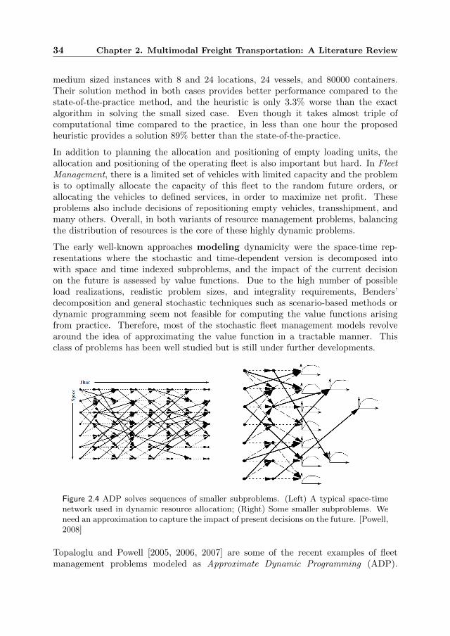
34 Chapter 2. Multimodal Freight Transportation: A Literature Review
medium sized instances with 8 and 24 locations, 24 vessels, and 80000 containers.Their solution method in both cases provides better performance compared to thestate-of-the-practice method, and the heuristic is only 3.3% worse than the exactalgorithm in solving the small sized case. Even though it takes almost triple ofcomputational time compared to the practice, in less than one hour the proposedheuristic provides a solution 89% better than the state-of-the-practice.
In addition to planning the allocation and positioning of empty loading units, theallocation and positioning of the operating fleet is also important but hard. In FleetManagement, there is a limited set of vehicles with limited capacity and the problemis to optimally allocate the capacity of this fleet to the random future orders, orallocating the vehicles to defined services, in order to maximize net profit. Theseproblems also include decisions of repositioning empty vehicles, transshipment, andmany others. Overall, in both variants of resource management problems, balancingthe distribution of resources is the core of these highly dynamic problems.
The early well-known approaches modeling dynamicity were the space-time rep-resentations where the stochastic and time-dependent version is decomposed intowith space and time indexed subproblems, and the impact of the current decisionon the future is assessed by value functions. Due to the high number of possibleload realizations, realistic problem sizes, and integrality requirements, Benders’decomposition and general stochastic techniques such as scenario-based methods ordynamic programming seem not feasible for computing the value functions arisingfrom practice. Therefore, most of the stochastic fleet management models revolvearound the idea of approximating the value function in a tractable manner. Thisclass of problems has been well studied but is still under further developments.
Figure 2.4 ADP solves sequences of smaller subproblems. (Left) A typical space-timenetwork used in dynamic resource allocation; (Right) Some smaller subproblems. Weneed an approximation to capture the impact of present decisions on the future. [Powell,2008]
Topaloglu and Powell [2005, 2006, 2007] are some of the recent examples of fleetmanagement problems modeled as Approximate Dynamic Programming (ADP).
2.3 Operational Planning Problems 35
Figure 2.4 gives an illustration of the essence of ADP problems. These studiesoffer a nice framework for modeling and solving a variety of real world problems,especially those including time windows or labor restrictions, by addressing themat the level of the local subproblem. Topaloglu and Powell [2006] extend previousworks on ADP models for fleet management to include heterogeneous resources andsubstitution among them. Their method uses a hybrid of linear and piecewise-linearapproximations of the value function. Topaloglu and Powell [2007] develop sensitivityanalysis methods for a stochastic dynamic fleet management model to compute thechange in the objective value in response to changes in fleet size and load availability.Topaloglu and Powell [2005] extend the dynamic resource allocation problem to adistributed decision-making case. They use nonlinear functional approximation tomodel the coordination of actions of different agents.
Basically, simulation and approximation are used as solution methodologies.Topaloglu and Powell [2005] solve instances with 20 locations, 200 vehicle, and upto 6000 orders, and claim that in the deterministic version of the problem, thesolutions are near-optimal, but in the stochastic version with random demands,centralized decision making is slightly more effective than distributed decision making.Topaloglu and Powell [2006] model and solve the problem with up to 60 locations,600 vehicles, and 4000 orders. The hybrid value function seems to perform the bestin the deterministic case, while a piecewise linear value function provides the bestsolutions in the stochastic case. Topaloglu and Powell [2007] propose an approachwhich does not need multiple simulations with different values of the model parameterwhich is an important advantage. They decompose their dynamic program intotime-staged sub-problems and by using an iterative improvement scheme; the valuefunction is obtained with approximation. These tests are done on problem sets with40 locations, 200 vehicles, and up to 3000 orders during their planning horizon.Topaloglu and Powell [2007] implement this procedure first for single vehicle typeand then extend it to the multiple vehicle type problem. Shi et al. [2014] transformtheir dynamic fleet management problem with uncertain demand and customerchosen service levels into a dynamic network with partially dependent random arccapacities, and then decompose the network recourse into a series of tree resourceproblems. Overall, ADP with good approximation of value function stands strongin solving fleet management problems with realistic sizes. Bouzaiene-Ayari et al.[2014] propose an ADP framework for a rail fleet sizing and routing problem, witha streamlined single commodity model, a more detailed multicommodity model, anda multiattribute model. They show that ADP is much faster than a state-of-the-artInteger Programming (IP) solver, and can provide solutions for large and complicatedproblems with several stochastic elements.
The itinerary replanning problems form the second group of operational planningproblems. They are concerned with optimally responding to real-time systemevolution, to maximize the service quality and therefore the marginal profit. Here,the notion of a planned solution does not make sense and the whole operation shouldcontinuously react and adapt in real-time [Crainic, 2003]. The updating procedure,

36 Chapter 2. Multimodal Freight Transportation: A Literature Review
its accuracy and speed have a major influence on the efficient performance. Moreover,a single model or a solution approach no longer is capable of handling these complexproblems. As such, there is a need to employ combinations of approaches, not onlyfrom the OR area, but also decision-making and computational sciences. van Heeswijket al. [2016] study a real-time multimodal transportation planning where a “best k-route” generating heuristic is used to find routes for each arriving orders, and aconsolidation heuristic is called to find the best re-consolidation option for this orderamong the previously planned orders.
There is no doubt that ICT as well as tracking technologies such as RFID opened upmany opportunities for carriers and shippers for a better trade. Crainic et al. [2009]and Caris et al. gives an overview of different developments and current technologicalchallenges in Intelligent Transportation Systems (ITS), both in hardware and softwareplatforms. ITS delivers precise information in matter of seconds, hence significantlyreduces the uncertainty at the terminals and for the next carriers of the loads [Crainicet al., 2009]. Most of the developments in this regard have been hardware-driven, andmore efforts are still needed to model and solve multimodal transportation planningproblems under real-time information in an integrated chain [Crainic et al., 2009, Cariset al.]. Zuidwijk and Veenstra [2014] is an example where the value of informationis quantified when choosing modes of transport. They construct Pareto frontiers anddiscuss the value of information is terms of efficiency and reliability. The Paretofrontier decisions range from decisions where a barge is deployed at a very late stageto reduce costs while accepting a low level of reliability, to decisions where containersare planned for truck transportation to enhance reliability while accepting highercosts [Zuidwijk and Veenstra, 2014].
In the recent literature, Bock [2010] and Goel [2010] address the real-time issuesinto their models. Bock [2010] introduces a real-time-oriented control approach forefficient consolidation, transshipment, and dynamic handling of disturbances suchas vehicle breakdown and accidents. Partial or total outsourcing of transportationservices is also allowed and rest times for truck drivers are enforced. There are twodifferent plans for dynamic update handling, namely, the relevant and the theoreticalplans. When the execution of the relevant plan takes place, at an adaptation phase,generated future modifications are tested with the theoretical plan and based onfuture decisions. This approach works in a rolling horizon fashion. The simulationproduces a future temporary optimization problem which solutions determine the nexttransportation paths of each request and vehicle at the end of current time interval.
From a different perspective, Goel [2010] studies the value of utilizing RFIDtechnology and visibility over shipments throughout a multimodal transportationnetwork of road and fixed-scheduled rail, with variable transit times. In this network,there are two decision-makers: a transport manager responsible for planning theshipments, and a terminal operator responsible for dealing with unforeseen deviations.If the manager does not see the deviations in time and adjust accordingly, the terminaloperator must then decide upon the shipment flows. Goel [2010] analyzes four levels

2.3 Operational Planning Problems 37
of visibility, namely, no visibility, daily snapshot, departure/arrival, and checkpoint.
In order to solve these itinerary planning problems, Bock [2010] designs a variableneighborhood search algorithm and solves generated instances with up to 5600locations, 372 orders, 399 transshipment locations, and 55 vehicles. He shows thatthe exact solutions are outperformed in a real-time environment and a continuousimprovement results in substantial cost reductions. Goel [2010] designs a simulationheuristic which at each iteration solves a multi-commodity network flow problembased on the updated information. He compare the defined visibility levels on a smallreal-world network of 1 supplier, 3 rail operators with up to 40 trains per operator,and 3 factories. Goel [2010] concludes that on-time delivery performance can besignificantly improved by increasing the level of visibility.
The number of papers on operational planning is remarkably lower than on thetactical and the strategic planning problems, opening many opportunities for futureresearch. We presented the highlights of the recent research. Operational planningproblems are huge, complex and heavily time consuming to solve. Huge sets of datashould be processed and new plans must be produced in matter of minutes or evenseconds. Better approximation, better decomposition of the problem, and tighterformulations can improve the performance of the DSS. Parallel computation andalgorithms also promise significant improvements in solving huge problems in matterof both time and efficiency. Moreover, the decision process and its timing might bealso interesting. Usually the decisions are made when the input data has arrived tothe system. For example, it is assumed that the arrival of a ship is announced rightwhen it arrives to a terminal. Planning the required operations beforehand mightsave both computational and execution times.
Moreover, in the operational planning literature, the modal switch is ignored. Assumethat for example, at some point a large volume order arrives, or there is a modalbreakdown. In such a situation, the choice of transportation mode and its operationalcosts are worth studying. In addition, no paper has discussed the dynamic allocationof multi-asset resources. In an international containerized transportation chain,usually more than one type of loading unit is used. For instance, reusable boxesor cages are allocated to customer orders, while the containers are allocated to movethese smaller units. Not only repositioning of empty containers is important, butreturning and positioning of empty smaller units is also important. Furthermore,incorporating transshipment time and capacity in terminals are interesting subjectsin resource management. Regarding empty loading units, it would be interesting toincorporate inventory and replenishment techniques to the ordering process of theseresources.

38 Chapter 2. Multimodal Freight Transportation: A Literature Review
2.4 Prospectives
Multimodal transportation has become the key platform for containerized trans-portation solutions. This chapter presented the recent developments and effortson multimodal transportation planning from 2005 onward. In overall, operationalplanning issues have been studied less than tactical ones, and many challenges stillremain.
First of all, transportation of time-sensitive products such as perishables requiremore study regarding their special transportation structures, policies, and objectives.Regarding transportation resources, there is a big gap in incorporatingthe backward flows into the planning of forward flows. The literature showsthat by integrating the repositioning decisions in the network design, solutions aresignificantly more cost efficient and time saving. Moreover, taking dynamicity andstochasticity of the data into account also remains a major research challenge.
In most papers, it is assumed that the transportation system is centrally managed andonly the requirements of the multimodal operator are taken into account. Obviously,the interactions and competitions among the carriers influence the execution of theplans. Their collaboration for example ensures the on-time delivery. Furthermore,integrating different levels of planning might provide more reliability, flexibility, andmore important sustainability, generating more efficient solutions for the industry.
For both planning levels, due to the complexity of the problems, solving them is stilla challenge in itself. Decomposition and relaxation techniques are used extensively.Branch-and-Cut algorithms provide a flexible platform to include many propertiesof network design problems, and with smart exploitation of the problem structure,finding stronger bounds and cuts, it is possible to push the size limits and solvemore realistic problems. Among the metaheuristic algorithms, the family of Tabusearch heuristics was used most. This fact leaves a great opportunity to studyother families of metaheuristic algorithms and compare their performance,especially in solving realistic problem sizes.
In this chapter, the different terminologies used in practice - multimodality, inter-modality, co-modality, and synchromodality - were also discussed. The latter twohave not received any attention from the OR community. However by looking attheir definition, synchromodality seems to be very appealing for the flexibility andefficiency it envisions. It offers a better utilization of transportation modes andresources, a better consolidation of loads, flexibility and freedom to switch modes,and synchronization of the services. These terms are in fact the essence of optimizedmultimodal transportation planning which needs to take many practical aspects intoaccount such as the collaboration of the administrative bodies, uncertainty, trafficat terminals or en route, resource limitations and modal capacities. To conclude,despite the fact that the research in the area of multimodal transportation planninghas accelerated, we believe that this outline and review gives ample new researchdirections for future study.

2.4 Prospectives 39
The following chapters of this thesis build upon and adds to this literature by studyingthe multimodal transportation planning for perishable product industries with theirown characteristics and complexities.

40 Chapter 2. Multimodal Freight Transportation: A Literature Review
Part II
Tactical Planning

Chapter 3
A MIP for MultimodalLong-haul Transportation ofPerishable Products withEmpty Repositioning
The transportation planning problems studied in this thesis are grouped intotactical and operational planning problems. The current chapter aims to framethe tactical planning problem, its elements and structure. Such a problem is anextension to the classic Fixed-charge Capacitated Multicommodity Network FlowProblem (FCMNFP), where additional sets of constraints related to product qualitypreservation and management of Returnable Transport Items (RTIs), are added tothese problems. Due to complexity of this problem however, in this chapter, only onesize of RTI is included. Section 3.1 gives a comprehensive description of this problem,and Section 3.2 recalls the relevant literature. Sections 3.3, and 3.4 provide themodeling approaches, and the mathematical formulation which is tested and solvedby a state-of-the-art solver in Section 3.5. Finally, in Section 3.6, some concludingremarks are provided.
3.1 Problem Description
Tactical planning deals with utilizing a given transportation infrastructure bychoosing the best services and associated transportation modes, efficient allocationof their capacities to customer orders, and management of all resources involved. Ontactical planning level, information on availability of resources, customer demand,

44 Chapter 3. A MIP for Long-haul Transportation of Perishable Products
Figure 3.1 The tactical planning problem for a perishable transportation system
and service costs are usually aggregate, and the tactical solutions give insights to theplanners and operators on how to efficiently utilize the available fleet and resources fora particular time span or horizon. This planning horizon can be one week, one month,one season, etc. Figure 3.1 illustrates the tactical planning problem of multimodallong-haul transportation of perishable products, showing its inputs, output, decisions,objective function, and its constraints.
The main decisions are the flows of products (customer demand), the repositioning ofRTIs, and the selection of transport modes and schedules to do them. To furtherexplore these decisions and the constraints applied on them, it is necessary tounderstand the role that RTIs play in the transportation, and how customer demandis defined into the system.
Returnable Transport Items (RTIs), being the loading units used for transportation,are the key elements to model this problem, and the main decisions are defined ontheir “flow” throughout the network. Their number throughout the network is limitedand their flow is subjected to strict resource balance constraints. For instance, thenumber of RTIs available at the beginning of the planning horizon should be equalto their number at the end of horizon. The initial number of RTIs however is given,and its value is not a decision. There are three reasons making RTI managementdifferent from managing the fleet of vehicles which has been widely studied in theliterature. First, the number of RTIs (e.g. cages, Dense fusters, staple wagons,trolleys) around the network is usually much larger than the number of vehicles (e.g.trucks). Consequently, indexing an RTI in the modeling like how it is done for vehicles,would result in an enormous intractable model. Furthermore, if there is more thanone storage center for the empty RTIs, it is usually not important to return an RTI tothe same location where it was loaded. In general, vehicles need to return to the same

3.1 Problem Description 45
location they started their travel, while the only requirement for RTI managementis, for instance, to have as many RTIs at the end of a planning horizon as there wasat the beginning. In other words, RTIs are anonymous. These reasons make RTImanagement unique.
Demand is here represented by orders. An order is characterized by its pair oforigin and destination locations, its volume, its pickup and delivery schedules, andits freshness requirements. Since RTIs are the loading units used to transport theproducts, the order volume shows the number of RTIs (e.g. 2 trolleys) needed totransport products from the origin to the destination. The products can be pickedup and loaded onto the RTIs at an earliest given time, and should be delivered to thedestination and unloaded at an latest given time. These schedules are not definitethough, and as long as the order is transported within the length of this schedule,its flow is feasible. For instance, an order might be held for a few hours at itsorigin location before it is loaded and transported. Besides management of RTIs, theother factor adding extra complexity to this problem is preserving product qualityand delivering the desired freshness to its market. Perishable products lose their valueover time, and due to geographic distances between production sites and final markets,preserving product quality is a determining factor in all transportation decisions.However, measuring and controlling the health of products are not straightforward. Inthe horticultural supply chain of the Netherlands, product freshness is approximatedby a Time Temperature Sum (TTS) measure, and a maximum limit is enforced onTTS of orders.
Typically, demand in a FCMNFP problem is defined as commodities, and the onlyflow decision is defined on their routing throughout the network. However, in thisproblem, there are three types of flow decisions:
1. laden flow decisions for loaded RTIs that are transporting the products,
2. assign flow decisions for empty RTIs that are repositioned from a location withsurplus of RTIs, to the origin locations of orders to be assigned to their transport,
3. repos flow decisions for empty RTIs that are repositioned from the destinationlocations of orders back to the storage locations with RTI shortage.
Both assign and repos flow decisions are about empty RTIs, however, for modelingpurpose, they are defined separate. This separation though does not increase thecomplexity of the problem.
In order to transport full and empty RTIs, from the available fleet of differenttransportation modes, the modes and schedules doing the job, should be decided.These decisions not only include transportation activities, but also include handlingand holding activities. All transport modes and all hub locations have giventemperatures, which are included in computing the quality measure. Note that the

46 Chapter 3. A MIP for Long-haul Transportation of Perishable Products
temperature of a mode shows for example, the temperature inside a truck trailer, atrain car, or a barge storage room.
About the multimodal transportation fleet, each transport mode has given schedules,and its vehicles operate based on these schedules (e.g. trains depart from a hublocation every 6 hour). Moreover, vehicles of a transport mode are capacitated (here,based on RTIs), and there are limited number of vehicles available for each transportmode. These restrictions make the planning problem more complex and have majorinfluence on transporting the RTIs.
Objective functions of tactical planning problems can have different forms, dependingon the planner’s choice of performance indicators. These indicators can be financial, ordefined based on customer satisfaction measures, etc [Parmenter, 2007]. In perishableindustries for instance, as described earlier, maximizing the freshness of deliveredproducts or minimizing the number of perished products at delivery, can be anobjective function. In the majority of planning problems though, financial indicatorsare used. In this thesis, operational costs are the key indicators, and the objectivefunction of this problem is to minimize the total system costs. Costs of renting a truckor reserving space (capacity) on a freight train, costs of handling (loading, unloading,or transshipping) products or RTIs, costs of storing them, administrative costs of theseoperations, etc., are examples of operational costs in such a transportation system.If there are defined penalties on failing to provide customers’ requested productfreshness, they can also be added to the objective function. In the horticultural sectorof the Netherlands though, the product freshness constraint is strict and no perishedproduct at delivery is accepted. This constraint can be translated into enforcinginfinite penalty costs on the perished products.
3.2 Related Literature
Section 1.2 discussed the literature of long-haul transportation of perishable products.Reis and Leal [2015] propose a MIP model for a soybean shipping chain planningproblem where choice of transportation mode is included in the model besidesdecisions for annual crop purchase. Since their real-world application deals withsignificant uncertainty related to crop production, they define several combinations ofscenarios for this uncertainty and apply their MIP model to each scenario in order togive insights to their decision makers. Bortolini et al. [2016] propose a tri-objective LPfor tactical planning of a food distribution network considering operating cost, carbonfootprint and delivery time goals. They apply their tool to a real-world distributioncase and show the trade-off between the operational costs and the carbon footprint.This chapter adds to this literature by incorporating management of resources, hereRTIs, which is missing in Reis and Leal [2015] and Bortolini et al. [2016].
On multimodal freight transportation in general, Section 2.2 provided an overviewon the recent tactical planning modeling and solution design advances. Optimal

3.3 Modeling Approach 47
tactical solutions comprise the optimal and timely utilization and operation of itsresources, called assets. Assets can be RTIs, vehicles, crews, power units, engines, etc.,and positioning, balancing, allocating, repositioning, and rotation of assets are thesubject of asset management. Repositioning of vehicles has been widely investigatedin the literature, mostly addressed as Service Network Design (SND) problems, andexamples are Pedersen et al. [2009], Andersen et al. [2009a], Andersen et al. [2009b],and Andersen et al. [2011], Li et al. [2016], and Demir et al. [2015].
The number of studies managing loading units such as RTIs is very limited. Braekerset al. [2013] and Meng and Wang [2011] are the two examples found in the literaturewhere empty container repositioning is included into liner shipping service design.However, in both papers, the repositioning orders are given and pre-defined, andcan be treated as additional customer orders besides the usual ones. From anotherperspective, Choong et al. [2002] model the flow of owned and leased empty containerson barges, investigate 15-day and 30-day planning horizons. Choong et al. [2002]however do not study the integration of empty repositioning and forward flow ofproducts. The current chapter adds to the literature of FCMNFP problems byincluding RTI management decisions. In the next section, the modeling approachis described in detail.
3.3 Modeling Approach
In modeling this problem, first, two main elements need to be explored: 1) thestructure of network and its resources, and 2) evaluating and incorporating productquality. Appendix B provides a summary of all notations used.
3.3.1 Mode-Space-Time Network Representation
The physical transportation network is characterized by nodes i ∈ N representingthe hub locations, and the arcs (i, j) representing different routes connecting theselocations. Between each location pair, at least one transportation mode m ∈{1, . . . ,M} can operate. Truck, train, and barge are examples of possible modes.
In order to include all activities such as handling and holding operations into themodel, the physical network is transformed into a mode-space-time representation.First, the time horizon T (e.g. 48 hours) is divided into a set of time periods t =1, . . . , T (e.g. an hour), and the physical network is mapped in both time and space.Each node in such a network represents a location at a time period. Of course, timehas a continuous nature, and discretizing it is not the only modeling approach. Incontinuous-time models, modeling the precedence of loading, unloading, transporting,and other activities, and their scheduling synchronization is difficult, especially in thecontext of multimodal transportation, where some modes such as trains and bargeshave their own timetables. In comparison, in discrete-time models, if t is really small

48 Chapter 3. A MIP for Long-haul Transportation of Perishable Products
compared to T (e.g. t has a length of one minute and T is a month), the size of thenetwork will be too large to handle for any MIP solver. However, in this problem,length of activities are usually aggregated to e.g. hourly scales, and the time variablein the product freshness measure is not continuous. Therefore, in this thesis, the timedimension was discretized.
Afterwards, the space-time mapping is furthermore copied M+ 1 times, where eachnode v ∈ V in this new network represents a location i ∈ N at a time t ∈ {1, . . . , T}period on a mode m ∈ {1, . . . ,M + 1}. Layers m = 1, . . . ,M can accommodateall transport activities, whether with fixed timetables or flexible, but the extra layerof m = M + 1, here called holding mode H, is added to represent the handlingand holding activities. Figure 3.2 gives an illustration of a simple mode-space-timenetwork with 3 locations, 16 time periods, and 2 modes. In this example, a feasibleflow itinerary for an order from location 1 to location 3 with PT of 5 and DT of 9 isshown. All empty RTIs are kept at location 2, and at the end of planning horizon,their total number should be equal to their initial number. For the order, the neededRTIs are first loaded to vehicles of mode 2, transported from location 2 to location 1,and unloaded at location 1 at time 4. Then the RTIs are filled and loaded to vehiclesof mode 1, moved to location 3, and unloaded at location 3 at time 7. After unloadingand emptying the RTIs, they are returned to their storage location via mode 2 in asimilar fashion, and are kept for the final 2 consecutive periods.
Figure 3.2 An example of the mode-space-time representation of a flow network problem
The mode-space-time network has the flexibility to accommodate any type of
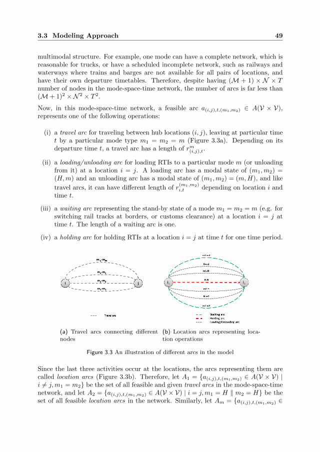
3.3 Modeling Approach 49
multimodal structure. For example, one mode can have a complete network, which isreasonable for trucks, or have a scheduled incomplete network, such as railways andwaterways where trains and barges are not available for all pairs of locations, andhave their own departure timetables. Therefore, despite having (M + 1) × N × Tnumber of nodes in the mode-space-time network, the number of arcs is far less than(M+ 1)2 ×N 2 × T 2.
Now, in this mode-space-time network, a feasible arc a(i,j),t,(m1,m2) ∈ A(V × V),represents one of the following operations:
(i) a travel arc for traveling between hub locations (i, j), leaving at particular timet by a particular mode type m1 = m2 = m (Figure 3.3a). Depending on itsdeparture time t, a travel arc has a length of rm(i,j),t.
(ii) a loading/unloading arc for loading RTIs to a particular mode m (or unloadingfrom it) at a location i = j. A loading arc has a modal state of (m1,m2) =(H,m) and an unloading arc has a modal state of (m1,m2) = (m,H), and like
travel arcs, it can have different length of r(m1,m2)i,t depending on location i and
time t.
(iii) a waiting arc representing the stand-by state of a mode m1 = m2 = m (e.g. forswitching rail tracks at borders, or customs clearance) at a location i = j attime t. The length of a waiting arc is one.
(iv) a holding arc for holding RTIs at a location i = j at time t for one time period.
(a) Travel arcs connecting differentnodes
(b) Location arcs representing loca-tion operations
Figure 3.3 An illustration of different arcs in the model
Since the last three activities occur at the locations, the arcs representing them arecalled location arcs (Figure 3.3b). Therefore, let A1 = {a(i,j),t,(m1,m2) ∈ A(V × V) |i 6= j,m1 = m2} be the set of all feasible and given travel arcs in the mode-space-timenetwork, and let A2 = {a(i,j),t,(m1,m2) ∈ A(V × V) | i = j,m1 = H ‖ m2 = H} be theset of all feasible location arcs in the network. Similarly, let Am = {a(i,j),t,(m1,m2) ∈

50 Chapter 3. A MIP for Long-haul Transportation of Perishable Products
A(V ×V) | m1 = H ‖ m2 = H} be the set of all feasible loading, unloading, traveling,and waiting arcs in the network related to mode m.
3.3.2 Modeling Quality Preservation
Modeling quality and evaluating the shelf life are not straightforward. There isno standard model, showing how product quality changes over the course of itstransportation. There are various physical, chemical, and biological factors involved.Most perishable industries resort to simple rules of thumb, based on e.g. color, smell,weight, etc., and define quality classes, and by experience, label products in therelevant classes.
In practice, quality is translated as how much customers are willing to pay for it.This value also depends on the type of product, the market it is sold to, seasonality,etc., and it is not computed easily. Customers’ desired freshness (e.g. how much arose bud is open, or how mature a cheese product is) has different prices in differentmarkets.
Shelf life of a product is the length of time after which products are perished and haveno value. In modeling product quality, if product value is constant over its shelf life,e.g. for blood [Doerner et al., 2008], quality preservation is modeled as a constraint.Otherwise, a product quality loss function is defined and relevant penalties for qualitydecrease is added to the main objective function of the planning problem [Ahumadaand Villalobos, 2011, Hsu et al., 2007].
As reviewed in Section 1.2, the literature hardly includes temperature conditions inthe quality control modeling. In horticultural industry of the Netherlands, productfreshness is approximated by a Time Temperature Sum (TTS) measure. TTS isa measure used in some industries representing the total time that products can betransported in different temperature regimes [Sloof and Everest, 2001, Taoukis, 2001].For instance, if a loaded RTI is moved on a train for 5 hours and the temperatureinside the train is 10 degree Celsius, the TTS of this travel is 50, and a maximumallowed TTS (e.g. 200 hour-degree) is enforced for each order. This limitation isadded to the model via a new set of constraints. In the remainder of this section, theMIP is presented.
3.4 Mathematical Model
In this section, the mathematical formulation for the multimodal network flowproblem with product quality preservation and management of RTIs is explained.
Section 3.3.1 discussed about why continuous modeling approach is not used in thisthesis. In the literature of FCMNFP problems, there are three types of discreteformulations:

3.4 Mathematical Model 51
� arc-based formulations, where asset-related decision variables are defined onnetwork arcs,
� path-based formulations, where asset-related decision variables are defined onnetwork paths,
� cycle-based formulations, where assets have cyclic paths, and their relateddecision variables are defined on cycles.
Cycle-based formulations are suitable for service network design problem, whereservices are cyclic and there are design-balanced constraints in the problem. Here,services are not owned by the planner, therefore, cycle-based formulations are notuseful.
In path-based formulations, the set of all possible paths between each pair of nodesin the mode-space-time model are generated, adding new variables and constraints tothe formulations. Path-based formulations might outperform arc-based formulations[Andersen et al., 2009b], but in this research, the number of modes and their fixedschedules over the length of the planning horizon, exponentially increase the sizeand the computing efforts of generating this set. of this set. Therefore, arc-basedformulation is used in this research.
An order p is characterized by its origin O(p), its destination D(p), volume wp, anearliest pickup time of PT (p), a latest delivery due date of DT (p), and the maximumallowed TTS of Lp.
Each transport mode m ∈ {1, . . . ,M} has its given schedules, its speed speedm,vehicle capacity capm, total Fm number of available vehicles, and a temperature lm.In this problem, costs associated with each transport mode are the fixed costs of usinga vehicle (or its available capacity) Cm, and the variable costs of Cmladen per loadedRTI per time period, and Cmempty per empty RTI per time period.
Each location i is assumed to have a temperature li,t at time t, and a unit holdingcost of Choldi per RTI. Moreover, each location i is assumed to have Si ≥ 0 numberof RTIs available at the beginning of the planning horizon, and the number of RTIs
at the end of horizon should be equal to the initial value of Si. Let C(m1,m2)i be the
general term for loading, unloading, and holding costs per RTI per time period, whichare enforced on the location arcs.
As described earlier, for each order p, there are three flow decisions in this problem:laden, assign, and repos flow decisions. In this mode-space-time network, for eachflow decision, two sets of decision variables are defined: 1) x to show how many RTIsenter an arc a(i,j),t,(m1,m2), and 2) x to show how many RTIs exit the arc. It wouldhave been easier to model, if an extra index t′ was added to the (i, j), t, (m1,m2)indices, in oder to distinguish the starting and the finishing times of a travel or anoperation, and define only one x variable set. However, this model has in total T/2times less variables, which reduces the size of the model.

52 Chapter 3. A MIP for Long-haul Transportation of Perishable Products
Similarly, there are two sets of variables y and y to show the number of vehiclesrespectively entering and exiting an arc. The auxiliary binary variables b and b arealso added to help calculating TTS.
Three categories of variables U are added to the model to keep track of the inboundand outbound flows at each location, and to connect the flows of loaded and emptyRTIs throughout the network.
Returning to the example illustrated in Figure 3.2, Figure 3.4 shows the positive xflow variables in the example. Certainly, an equal number of x, b, and b variables arepositive as well, and their equivalent y and y variables equal to at least 1. Note thatin an example with higher number of orders, if the capacity of vehicles does not allowfor consolidation, y and y might be bigger.
Figure 3.4 Positive flow variables in the example of Figure 3.2
The FCMNFP problem with product quality preservation and empty RTI manage-ment is then formulated as follows:
The objective function is in the form of minimizing total system costs, where theterm (3–1a) represent flow costs of the loaded RTIs, the terms of (3–1b) are the flowcosts of the assigned and repositioned empty RTIs respectively, the term (3–1c) showslocational costs of loaded RTIs, the terms (3–1d) represent locational costs of assignedand repositioned RTIs, and finally, (3–1e) shows the costs of using the modes.
Constraints (3–2)-(3–7) match pairs of entering and exiting variables, to ensurenetwork arc connectivity. Constraints (3–8) are flow conservation constraints. Theseconstraints define variables U as the total network flow (loaded RTIs, assigned empty

3.4 Mathematical Model 53
and repositioned empty RTIs) for each order at each location and time period.
min
∑a(i,j),t,(m1,m2)∈A1
rm(i,j),t
P∑p=1
Cmladen
(xladenp,(i,j),t,(m1,m2)
) (3–1a)
+∑
a(i,j),t,(m1,m2)∈A1
rm(i,j),t
P∑p=1
Cmempty
(xassignp,(i,j),t,(m1,m2)
+ xreposp,(i,j),t,(m1,m2)
) (3–1b)
+∑
a(i,j),t,(m1,m2)∈A2
r(m1,m2)i,t
P∑p=1
C(m1,m2)i
(xladenp,(i,i),t,(m1,m2)
) (3–1c)
+∑
a(i,j),t,(m1,m2)∈A2
r(m1,m2)i,t
P∑p=1
C(m1,m2)i
(xassignp,(i,i),t,(m1,m2)
+ xreposp,(i,i),t,(m1,m2)
) (3–1d)
+
M∑m=1
∑a(i,j),t,(m1,m2)∈Am
Cm × y(i,j),t,(m1,m2) (3–1e)
xcatp,(i,j),t,(m1,m2) = xcat
p,(i,j),(t+rm(i,j),t
),(m1,m2)
∀cat ∈ {laden, empty, repos},a(i,j),t,(m1,m2) ∈ A1
p = 1, . . .P(3–2)
xcatp,(i,i),t,(m1,m2) = xcat
p,(i,j),(t+r(m1,m2)i,t ),(m1,m2)
∀cat ∈ {laden, empty, repos},a(i,j),t,(m1,m2) ∈ A2
p = 1, . . .P(3–3)
y(i,j),t,(m1,m2) = y(i,j),(t+rm(i,j),t
),(m1,m2) ∀a(i,j),t,(m1,m2) ∈ A1 (3–4)
y(i,i),t,(m1,m2) = y(i,j),(t+r
(m1,m2)i,t ),(m1,m2)
∀a(i,j),t,(m1,m2) ∈ A2 (3–5)
bp,(i,j),t,(m1,m2) = bp,(i,j),(t+rm(i,j),t
),(m1,m2)∀a(i,j),t,(m1,m2) ∈ A1
p = 1, . . .P (3–6)
bp,(i,i),t,(m1,m2) = bp,(i,j),(t+r
(m1,m2)i,t ),(m1,m2)
∀a(i,j),t,(m1,m2) ∈ A2
p = 1, . . .P (3–7)
Ucatpit =
∑j∈V−{i}
∑t′>t
M+1∑m=1
xcatp,(i,j),t,(m1,m2)
−∑
j∈V−{i}
∑t′<t
M+1∑m=1
xcatp,(j,i),t,(m1,m2)
∀cat ∈ {laden, empty, repos},i ∈ V,t = 1, . . . , Tp = 1, . . .P
(3–8)
Constraint set (3–9) enforces the flow of loaded RTIs (orders) between origin anddestination locations. It enforces the outbound flow of an origin node to be wp andthe inbound flow of a destination node to be −wp. Note that even though Constraints(3–9) are equality constraints, there is no obligation for an order to immediately beloaded and transported at its earliest pickup time. In a feasible solution, an order

54 Chapter 3. A MIP for Long-haul Transportation of Perishable Products
might be held for several time periods before loading. Similarly, the delivery due dateof an order is not definite.
U ladenpit
= wp i = O(p), t = PT (p)= −wp i = D(p), t = DT (p)= 0 o.w.
∀i ∈ V,t = 1, . . . , Tp = 1, . . .P
(3–9)
Uassignpit
≤ Si Si > 0, t = 0= −wp i = O(p), t = PT (p)0 o.w.
∀i ∈ V,t = 1, . . . , Tp = 1, . . .P
(3–10)
Urepospit
= wp i = D(p), t = DT (p)≥ −Si Si > 0, t = T0 o.w.
∀i ∈ V,t = 1, . . . , Tp = 1, . . .P
(3–11)
Constraints (3–10) and (3–11), in a similar fashion enforce the flow of empty RTIsbetween origin and destination locations. The origin locations of the assigned emptyRTIs are the RTI storage locations with Si > 0. Their destination locations are thelocations that they are needed to be loaded and transport the products (O(p),PT(p)).On the other hand, the repositioned empty RTIs need to get back to the storagelocations. Therefore, the locations with Si > 0 are their destinations and theirorigin locations are the locations that the loaded RTIs are unloaded (D(p),DT(p)).Constraint set (3–12) enforces the number of empty RTIs at a storage locations atthe beginning of the planning horizon to to be equal to the number at the end of theplanning horizon.
∑j∈V−{i}
M+1∑m=1
P∑p=1
xassignp,(i,j),0,(m1,m2)
=∑
j∈V−{i}
M+1∑m=1
P∑p=1
xreposp,(j,i),T,(m1,m2)
∀i ∈ V : Si > 0
(3–12)
Constraints (3–13) and (3–14) are logical constraints which are used to calculate theTTS of orders. Note that M here is the classic “big M” and not the set of modes.Based on these constraints then, if there is no flow of products on a specific arc(x = 0), that arc will not be included in the constraint on TTS (b = 0).
xladenp,(i,j),t,(m1,m2) ≥ bp,(i,j),t,(m1,m2)
∀a(i,j),t,(m1,m2) ∈ A(V × V),p = 1, . . .P (3–13)
xladenp,(i,j),t,(m1,m2) ≤ Mbp,(i,j),t,(m1,m2)
∀a(i,j),t,(m1,m2) ∈ A(V × V),p = 1, . . .P (3–14)
Based on Constraints (3–13) and (3–14), Constraint set (3–15) states that for eachorder, the total time × temperature of moving and handling an order must be lessthan or equal to its required TTS.

3.4 Mathematical Model 55
∑a(i,j),t,(m1,m2)∈A1
lm(i,j),t × rm(i,j),t × bp,(i,j),t,(m,m)
+∑
a(i,j),t,(m1,m2)∈A2
l(m1,m2)i,t × r(m1,m2)
i,t × bp,(i,i),t,(m1,m2) ≤ Lp ∀p = 1, . . .P (3–15)
Constraint (3–16) is the capacity constraint. The total number of RTIs (laden orempty) that is moved between i and j at time t should be less than or equal to thetotal capacity of y vehicles of mode m transporting them, if that mode is chosen.
P∑p=1
xladenp,(i,j),t,(m1,m2) +
P∑p=1
xassignp,(i,j),t,(m1,m2)
+
P∑p=1
xreposp,(i,j),t,(m1,m2)
≤ capm × y(i,j),t,(m1,m2) ∀a(i,j),t,(m1,m2) ∈ Am (3–16)
Let At,m = {a(i,j),t,(m1,m2) ∈ A(V ×V) | m1 = m,m2 = m, t ≤ t ≤ t} be the set of allarcs of mode m ∈ {1, . . . ,M} crossing time period t. Constraint (3–17) then statesthat in each time period, the number of used vehicles of a mode type must be lessthan or equal to a maximum value Fm.
∑a(i,j),t,(m1,m2)∈At,m
y(i,j),t,(m1,m2) ≤ |Fm|∀t = 1, . . . , T,m = 1, . . . ,M (3–17)
Finally, Constraints (3–18)-(3–20) define the nature of the variables in the formula-tion.
xcatp,(i,j),t,(m1,m2), x
catp,(i,j),t,(m1,m2) ≥ 0
∀cat ∈ {laden, empty, repos},a(i,j),t,(m1,m2) ∈ A(V × V),p = 1, . . .P
(3–18)
bp,(i,j),t,(m1,m2), bp,(i,j),t,(m1,m2) ≥ 0∀a(i,j),t,(m1,m2) ∈ A(V × V),p = 1, . . .P (3–19)
y(i,j),t,(m,m), y(i,j),t,(m,m) ∈ N ∀a(i,j),t,(m1,m2) ∈ A(V × V) (3–20)
Constraints (3–10), and (3–11) and their related flow conservation constraints are newto the literature of FCMNFP problems. Constraints (3–13), (3–14), and (3–15) whichrepresent product quality requirements are also new to the literature of FCMNFPproblems. In the next section, this formulation is tested on a number of instancesand its sensitivity to different parameter settings is analyzed.

56 Chapter 3. A MIP for Long-haul Transportation of Perishable Products
3.5 Numerical Experiments
In this section, the proposed formulation presented in Section 3.4 is verified ondifferent instances, the tactic used to strengthen and to speed up the computation isexplained, and then some practical insight is given. All instances are solved on a 2.4GHz CPU with 8.00 GB RAM, and Gurobi solver 6.5.0 is used as the MIP solver.The instances are run for a maximum time of 10 hours.
3.5.1 Instance Sets
The instance sets used in this thesis are extracted from the transportation ofhorticultural products on the Trans-European Transport Network (TEN-T) [Tosi,2014, Verhoeven, 2014, Vlassak, 2014, Rosenboom, 2014]. However, the number oflocations, the number of product types and the RTIs involved are enormous. To beable to test the model, the real network is aggregated to have only 20 hubs (Figure3.5), where two of them are inbound hubs and the rest are outbound hubs. Inboundhubs are locations where the products come from all around the world to get sold,sorted, and consolidated for the shipments. The outbound hubs on the other hand arelocations that the shipments are divided and packaged for the last-mile distribution.The instance are categorized in three groups of 7, 11, and 20 locations, where the firstgroup only includes only the hubs in the Netherlands, the second group includes thehubs in the Netherlands, Belgium and Luxemburg, and the third group includes allhubs.
Regarding the transportation modes, there are three classes of truck, train, andbarge transportation. Tables 3.1 gives the parameter setting for the modes. Thesenumbers have been extracted from company documents and annual EU reports ontransportation. As explained in Chapter 1, multimodal transportation is increasing,therefore, for the initial experiments, the multimodal network is assumed to becomplete, in order to see what modes are utilized in a restriction-free system. Later,these are compared with the case of a real-world network. In this table, Fm andcapm show the maximum number of available vehicles and their capacity for eachmode type. lm is the given temperature for each mode type based on degree Celsius.freqm shows that after how many hours, the next vehicle of each mode type departs,which is used as their fixed schedules. speedm shows the average speed of each vehiclebased on Km/Hr. Assuming Euro as the currency,Cm, Cmladen, and Cmempty are fixedcosts of using a vehicle, variable costs of transporting full RTIs per hour, and variablecosts of transporting empty RTIs per hour, respectively.
Without loss of generality, and by observing the practice, it is assumed that theempty RTIs in this network are stored at the inbound hubs. Due to the fact that therepositioning of medium-sized RTIs (e.g. cages, Dense fusters, staple wagons, trolleys)are critical in the horticultural chain, the chosen RTI will be the medium-sized RTI.Therefore, all numbers such as the number of RTIs in an order, the capacity of modes

3.5 Numerical Experiments 57
Figure 3.5 The horticultural network of hubs around the Europe; the white squares showthe inbound hubs, and the red circles represent the outbound hubs
Table 3.1 Transportation mode inputs
m Fm capm lm freqm speedm Cmfix Cmfull Cmempty
Truck services 200 22 5 1 65.00 136.34 6.412 2.849Train services 100 1760 5 6 32.50 179.37 0.025 0.011Barge services 100 704 5 2 18.52 118.04 0.008 0.004
per RTI, etc. are based on medium-sized RTIs. In this chapter, each inbound hub isassumed to have 12000 empty RTIs.
Finally, in order to generate the set of orders, a simple algorithm first randomly picksan origin from the inbound hubs, a destination from the outbound hubs, and theorder volume based on the demand information of the horticultural chain for eachdestination. Then, assuming the time horizon to be 48 or 72 hours, it randomlychooses the pickup time of the order. In the horticultural chain, customers demand12-hour, 24-hour, or 48-hour delivery service, therefore, delivery time of the ordersare chosen based on this scheme and by looking at the distances, the TTS (which isassumed to be 200), and the time that it takes to procure the needed empty RTIsand transport them to the origin, and the time needed to reposition them.
The instances are named as “nAmBtCoD” where value of A shows the numberof locations, value of B is the number of mode types, value of C is the planninghorizon, and value of D stands for the number of orders. In the following sections,
58 Chapter 3. A MIP for Long-haul Transportation of Perishable Products
computational results and some sensitivity analysis are presented.
3.5.2 Computational Strengthening
Balakrishnan et al. [1997] have shown that the fixed-charge capacitated network designproblem is NP-hard. This problem incorporates additional product preservation andresource management decisions and constraints which add further complexity to theproblem. The number of decision variables goes very quickly beyond what can besolved to optimality with a state-of-the-art MIP solver. In the instance n7m1o10,there are 3222 arcs, and 25776 decision variables with positive cost coefficients in theobjective function. This is already larger than the majority of the existing instances inthe FCMNFP literature. Keeping all the matrices can cost a huge amount of memory.To deal with huge matrices of the parameters and variables that are extremely sparse,and to decrease the memory consumption of Gurobi, the so-called “colt”1 library isused to replace the standard matrix format with a sparse one. Colt libraries are a setof JAVA libraries designed for efficient use of scientific and technical data structureand algorithms, such as in multi-dimensional arrays, Monte Carlo simulations, etc.In multi-dimensional matrices for instance, it helps structuring the data such that itsmemory consumption is minimized.
3.5.3 Results
Tables 3.2 gives an overview of the results, including the obtained upper boundswithin 10 hours, the optimality gap, and some statistics on the multimodal fleet.
As shown in the table, Gurobi solver is not able to find the optimal solution of themajority of instances in 10 hours. In the group of n20, despite using “colt” library,Gurobi solver runs out of memory either during the construction of the model, orsolving the relaxation of the model. The computation time depends not only on thenumber of orders, but on the number of modes and the tightness of delivery times.Only for three instances with loose time windows, Gurobi was able to find a feasiblesolution in ten hours without running out of memory.
In this table, the number of vehicle used for each mode, their average utilization, andthe share of each mode in transporting the total flow in the solution are presented.Note that the instances with m1 only have truck options, the instances with m2 havetruck and train options, and the instances with m3 have all three modes available.The objective function presents the total system costs including total fixed costs, costsof transporting loaded RTIs and costs of repositioning empty ones.
Since the main share of costs belongs to the fixed costs of using the modes, thecombination of fleet and the number of vehicles for each transportation mode is
1http://acs.lbl.gov/software/colt/

3.5 Numerical Experiments 59
Table 3.2 Initial results
Exact (10 Hours) Number of Vehicles Avg. Vehicle Utilization (%) Total Share of Flows (%)
n m t oUpperBound
Gap(%)
Comp.Time(seconds)
Truck Train Barge Truck Train Barge Truck Train Barge
n7 m1 t48 o10 55167 0.00 4423.44 84 - - 92.6 - - 100.0 - -n7 m2 t48 o10 1378b 0.00 1017.77 9 11 - 84.3 9.6 - 8.3 91.7 -n7 m3 t48 o10 13264 0.00 3269.28 9 4 7 84.3 2.3 34.7 8.2 8.0 83.8n7 m1 t48 o25 131248 0.61 10H 177 - - 95.4 - - 100.0 - -n7 m2 t48 o25 31112 0.00 4292.75 22 16 - 87.8 14.9 - 9.2 90.8 -n7 m3 t48 o25 30501 0.00 29218.80 22 8 8 87.8 12.0 44.3 9.2 36.7 54.1n7 m1 t48 o50 249644 0.28 10H 341 - - 97.1 - - 100.0 - -n7 m2 t48 o50 60992 0.00 23090.36 42 20 - 88.1 23.1 - 9.1 90.9 -n7 m3 t48 o50 60185 0.06 10H 42 9 11 88.1 15.1 60.7 10.3 30.3 59.4n7 m3 t48 o100 118265 0.38 10H 78 17 8 92.8 34.2 49.3 10.9 70.1 19.0n7 m3 t48 o200 228223 0.60 10H 157 24 14 94.0 56.3 60.2 9.8 72.1 18.0
n11m1 t48 o10 N.S. - - - - - - - - - - -n11m2 t48 o10 4507 0.01 5308.92 3 12 - 33.3 2.3 - 4.2 95.8 -n11m3 t48 o10 3775 12.20 10H 3 3 9 33.3 0.7 7.1 4.3 7.1 88.6n11m1 t48 o25 40827 0.73 10H 59 - - 76.1 - - 100.0 - -n11m2 t48 o25 14522 1.23 10H 14 18 - 52.9 3.3 - 13.3 86.7 -n11m3 t48 o25 13708 0.00 19912.06 14 8 10 52.9 3.3 8.5 13.3 37.8 48.9n11m1 t48 o50 81463 0.77 10H 101 - - 86.2 - - 100.0 - -n11m2 t48 o50 32185 0.00 10843.70 29 24 - 63.8 4.7 - 17.0 83.0 -n11m3 t48 o50 31489 1.13 10H 29 14 12 63.0 3.3 14.1 16.7 33.7 49.6n11m3 t48 o100 62862 2.99 10H 48 23 10 77.7 5.7 16.8 19.0 53.5 27.5n11m3 t48 o200 N.S. - - - - - - - - - - -
n20m1 t72 o10t N.S. - - - - - - - - - - -n20m2 t72 o10t N.S. - - - - - - - - - - -n20m3 t72 o10t N.S. - - - - - - - - - - -n20m1 t72 o25t N.S. - - - - - - - - - - -n20m2 t72 o25t N.S. - - - - - - - - - - -n20m3 t72 o25t N.S. - - - - - - - - - - -n20m1 t72 o50t N.S. - - - - - - - - - - -n20m2 t72 o50t N.S. - - - - - - - - - - -n20m3 t72 o50t N.S. - - - - - - - - - - -n20m3 t72 o100t N.S. - - - - - - - - - - -n20m3 t72 o200t N.S. - - - - - - - - - - -
n20m1 t72 o10l N.S. - - - - - - - - - - -n20m2 t72 o10l N.S. - - - - - - - - - - -n20m3 t72 o10l 10352.83 18.43 10H 7 9 11 78.6 3.3 11.1 8.1 34.7 57.3n20m1 t72 o25l N.S. - - - - - - - - - - -n20m2 t72 o25l 19723.48 18.33 10H 11 32 - 82.6 11.6 - 3.0 97.0 -n20m3 t72 o25l 18329.60 16.43 10H 11 18 15 82.6 6.6 35.0 3.3 34.9 61.8n20m1 t72 o50l N.S. - - - - - - - - - - -n20m2 t72 o50l N.S. - - - - - - - - - - -n20m3 t72 o50l N.S. - - - - - - - - - - -n20m3 t72 o100l N.S. - - - - - - - - - - -n20m3 t72 o200l N.S. - - - - - - - - - - -
Note: N.S. stands for “No Solution” and 10H is an abbreviation for 10 Hour time
interesting to investigate. Table 3.3 presents a summary of the number of vehiclesfor each mode type and the average percentage that each vehicle is utilized by theindustry targeted in this thesis. It shows that on average 52.8% of the time bargesare used and on average 17.4% of each barge is utilized by this sector. In contrast,trucks and trains are used 13.1% and 34.0% of the time, while on average 78.2% and5.9% of their vehicles are utilized by this sector respectively. This is due to cheapcosts of barge compared to the other two modes.
Overall, barge seems to be the most favorable means of transportation. However, invery large instances, trains have a bigger share of usage. They are expensive eventhough faster than barges, and only with a large number of orders they are cost-

60 Chapter 3. A MIP for Long-haul Transportation of Perishable Products
Table 3.3 An Overview of the Mode Usage in the Solutions
Average NumberAverage
Utilizationby this sector (%)
Average Usage (%)
truck train barge truck train barge truck train bargeo10 8 6 10 69.2 2.6 11.7 11.2 25.7 63.0o25 20 11 18 77.1 5.1 14.9 11.8 29.4 58.8o50 41 18 26 80.5 4.8 20.4 13.9 24.5 61.6
o100 72 31 38 84.8 6.4 24.9 14.2 29.9 55.9o200 160 44 62 86.7 12.1 29.5 14.5 31.5 54.0
o1000 174 134 133 75.4 4.9 11.0 12.7 45.2 42.0o2000 370 245 255 74.2 5.4 9.1 13.6 52.0 34.3
efficient.
One important issue is that the percentage of utilization of barges and trains by thissector in all instances is low. This is due to the fact that the products have strictdelivery requirements and these modes are mostly used for repositioning RTIs.
By increasing the number of orders for instance with the same number of modes andlocations,the usage of trucks and trains seems to increase, but the usage of bargesdecreases, even though the difference between usage of barges and the other two islarge (Figure 3.6). One important issue is that the utilization of barges and trucks inall instances is low. It can be argued that by increasing the number of orders further,the utilization of trains and barges will increase which also results in an increase intheir usage. In other words, larger flows and more volumes can result in a betterutilization of multimodal transportation system.
Looking at the total costs, the important trend seen is that by involving trains, andfurther barges, the total cost decreases even more than 50%. These results encouragethe usage of multimodal transportation.
Figure 3.6 Influence of the number of orders on the usage of the modes
From a computational point of view, it is clear that the problem is complex and toolarge to solve to optimality. Even in small sizes, the solver is not able to find theoptimal solution within 5 hours. In the group of n7 and n11, instances with more
3.6 Conclusions 61
than 50 orders cannot be solved, and in n20 instances, the ones with more than 14orders are not solved. Moreover, it is harder to find a solution for an order with tightdelivery of 12-hours. Likewise, it is harder to find a solution for m1 instances.
3.6 Conclusions
In this chapter, a multimodal network flow problem for long-haul transportation ofperishable products was developed, taking quality preservation, and asset manage-ment into account.
Multimodal transportation shows significant advantage in transporting perishableproducts. The model particularly integrates the repositioning of empty RTIs withthe flow of full ones to ensure the customer requirements are met. Multimodaltransportation results (for instances with m = 2, 3) in less costs compared to typicaltruck-only transportation (with m = 1). In addition, among different modes, bargesare mostly used, assuming the barge transportation infrastructure exists.
In total, the model was tested on 21 different instances with different number oflocations, up to 3 transportation modes, and up to 50 randomly generated order sets.The computational tactic that were used, helped decreasing the time and memoryissues with the huge matrices in the model. However, the memory problem still existsand solving instance with 50 orders and more is impossible. A fast and efficientheuristic is needed to solve more realistic sizes of instances with various constraintsand factors. Chapter 4 targets this issue by designing a solution algorithm that canhandle larger instances.
In addition, only one RTI size (e.g. trolleys) was used, and transportation of onlyone product type was planned. Appendix A extends the problem of this chapterto include three sizes of RTIs and their loading relations. It also provides somepreliminary results showing how complex it is. Since the problem with multiple assetsizes is relatively new to the literature, finding better models and algorithms for it isan interesting research direction.
Another extension is to plan for multiple product types, because some products areincompatible and need to be transported in compartments with different temperatureregimes.

62 Chapter 3. A MIP for Long-haul Transportation of Perishable Products

Chapter 4
An ALNS Metaheuristic forMultimodal Long-haulTransportation of PerishableProducts with EmptyRepositioning
Following Chapter 3, the current chapter addresses the tactical planning problemof multimodal long-haul transportation of perishable products. In Chapter 3, thisplanning problem was explored, and modeled as a Mixed Integer Program (MIP).Then, it was shown that the problem is very complex, and a state-of-the-art MIPsolver is not capable of providing solutions for its practical sizes. Therefore, thischapter builds upon the literature by proposing an Adaptive Large NeighborhoodSearch (ALNS) algorithm with new operators, improved scoring mechanism, and extrastrategies, to solve this complex problem. Section 4.1 gives a capsule description ofthe problem again, and Section 4.2 takes a look at the related literature of solutionalgorithms. In Section 4.3, the proposed solution algorithm, its properties, andstructure are described, and in Section 4.4, its performance is analyzed and comparedwith the results obtained in Chapter 3. Finally, in Section 4.5, some concludingremarks are provided.

64 Chapter 4. An ALNS for Long-haul Transportation of Perishable Products
4.1 Problem Description
Section 3.1 provides a detailed description of the multimodal transportation planningproblems with perishable products and repositioning of Returnable Transport Items(RTIs).
This problem is an extension of the classic Fixed-cost Capacitated MulticommodityNetwork Flow Problem (FCMNFP), and the main decisions are the flow of products(customer demand), the repositioning of RTIs, and the selection of transport modesand schedules to do these jobs.
RTIs are the key elements to model this problem, and the main decisions are definedon their flow throughout the network: 1) laden flow decisions for loaded RTIs thatare transporting the products, 2) assign flow decisions for empty RTIs that arerepositioned from a location with surplus of RTIs, to the origin locations of ordersto be assigned to their transport, and 3) repos flow decisions for empty RTIs thatare repositioned from the destination locations of orders back to the storage locationswith RTI shortage. The number of RTIs throughout the network is limited and theirflow is subjected to strict resource balance constraints.
Demand is here represented by orders. An order is characterized by its pair oforigin and destination locations, its volume, its pickup and delivery schedules, and itsfreshness requirements, which is evaluated by Time Temperature Sum (TTS) measure.
Fleets of different transportation modes are assumed available throughout thenetwork. Each transport mode has its given schedules, and its vehicles operatebased on them. For instance, trains depart from a hub location every 6 hours. Eachmode has a specific temperature, which for example shows the temperature inside atruck trailer, a train car, or a barge storage room. Vehicles of a transport modeare capacitated (here, based on RTIs), and there are limited number of vehiclesavailable for each transport modes. Besides transportation activities carried outby the available fleet, there are decisions implying the relevant handling or holdingactivities. Therefore, locations are also assumed to have their own temperature, whichis included in the quality measure of loading, unloading, and holding of laden RTIsat these locations.
Finally, the objective function of this problem is to minimize total system costs.Costs of renting a truck or reserving space (capacity) on a freight train, costs ofhandling (loading, unloading, or transshipping) products or RTIs, costs of storingthem, administrative costs of these operations, etc., are examples of operational costsin such a transportation system.
Balakrishnan et al. [1997] have shown that the capacitated fixed-charge network designproblem is NP-hard. This problem incorporates additional product preservation andresource management constraints and decisions, which add further complexity to theproblem. The number of decision variables goes very quickly beyond what can besolved to optimality with a state-of-the-art MIP solver. The results of Section 3.5

4.2 Related Literature 65
indicated this limitation as well.
4.2 Related Literature
The multimodal long-haul transportation planning problem in this research is a specialcase of FCMNFP problems. Figure 4.1 gives an overview of different approaches inthe literature to solve FCMNFP problems.
SolutionAlgorithms
Exact
Decomposition [Costa, 2005]
Relaxation [Thiongane et al., 2015]
Cutting-plane and Variable Inequalities [Costa et al., 2009, Chouman et al.,2011]
Branch-and-Price-and-Cut [Gendron and Larose, 2014]
Branch-and-Price local search [Hewitt et al., 2013]
Metaheuristicsand HybridHeuristics
Decomposition-based heuristic [Agarwal and Ergun, 2008, Garcıa et al., 2013,Li et al., 2016]
Cutting-plane based [Chouman and Crainic, 2014]
Evolutionary algorithm [Paraskevopoulos et al., 2016a]
Tabu search [Li et al., 2016, Pedersen et al., 2009]
MIP-tabu search [Chouman and Crainic, 2010, Yaghini et al., 2014]
Parallel Tabu search [Crainic et al., 2006]
MIP-local search [Hewitt et al., 2010, Rodrıguez-Martın and Salazar-Gonzalez, 2010]
Column generation based [Agarwal and Ergun, 2008, Brouer et al., 2014,Crainic et al., 2016, Karsten et al., 2016]
Slope scaling and ellipsoidal search [Zhu et al., 2014]
Figure 4.1 OR literature on solving Fixed-cost Capacitated Multi-commodity NetworkFlow Problem
Among the research works on exact solution algorithms, Costa et al. [2009] havestudied various inequalities, such as Benders, metric, and cutset inequalities.Chouman et al. [2011] also present a cutting plane algorithm where it implementsthe strong cover, minimum cardinality, flow cover, and flow pack inequalities. Theycompare and discuss the strength of each of these inequalities. On the other hand,Costa [2005] provide a review on the Benders decomposition techniques in differentnetwork design problems. Chouman and Crainic [2014] combine a cutting-planeprocedure with a variable-fixing procedure to solve their SND problem, embeddinga learning mechanism to the cutting-plane procedure to identify promising variables.Thiongane et al. [2015] apply several relaxation methods, such as Lagrangianrelaxation, linear programming relaxation, and partial relaxations of the integralityconstraints, and conclude that Lagrangian relaxation seems to offer a good tradeoffbetween the bound quality and the computation time. These exact solution algorithmsare only capable of solving really small instance sizes. The number of nodes, arcs,and commodities are not larger than 30, 700, and 400 respectively, while these valuesfor the smallest sizes of this problem are much larger.
Among metaheuristic algorithms, advanced Tabu Search (TS) algorithms have beenproposed the most. Pedersen et al. [2009] present a two-stage TS algorithm for the arc-based Design-Balanced Capacitated Multicommodity Network Design (DBCMND)
66 Chapter 4. An ALNS for Long-haul Transportation of Perishable Products
problem. The first stage of their TS explores the design-defined solution space viasingle-path-based neighborhoods. Then in the second stage, feasible solutions areidentified. Chouman and Crainic [2010] integrate mathematical programming witha TS algorithm for the FCMNFP problems. In their algorithm, the MIP with acutting-plane method computes lower bound, while the TS explores the solution spacefor upper bounds. They also propose a new arc-balanced cycle-based neighborhood.Yaghini et al. [2014] also introduce a new cutting-plane neighborhood into their TSmetaheuristic, which uses different strategies to select an open arc to be closed. Theyshow that their neighborhood outperforms many other methods such as cycle-based,path relinking, multilevel, and local branching methods.
These research works are not able to solve problems with more than 100, 000 variables,while in the smallest scale in this thesis, many more variables and constraints areincorporated. Therefore, an algorithm which can search the solution space fast butin a smart way is needed. Large Neighborhood Search (LNS) algorithms, and inparticular, Adaptive LNS (ALNS), have shown great performance for various large-scale transportation problems. ALNS was first introduced by Ropke and Pisinger[2006]. They propose an ALNS to solve a pickup and delivery problem withtime windows. Pisinger and Ropke [2007] later propose a more general ALNS tosolve various problems including the Vehicle Routing Problem with Time Windows(VRPTW) and the Capacitated Vehicle Routing Problem (CVRP). ALNS has beenwidely applied to VRP problems, but it is also gaining attention in other areas.Examples are Grangier et al. [2016] for solving a two-echelon VRP with multi-tripsat the second echelon, Gharehgozli et al. [2014] for scheduling twin automated cranesin a yard, Hemmati et al. [2016] for solving the inventory-routing with heterogeneousfleet of ships, Mauri et al. [2016] for a berth allocation problem, Rifai et al. [2016] forthe distributed permutation flow shop scheduling problem with multiple factories, andCanca et al. [2017] for solving a nonlinear location-routing problem, to design of rapidrail transit network. ALNS is relatively new to the literature, and its capabilitiesand limitations are still under investigation. It has not been applied to FCMNFPproblems, therefore, this chapter adds to the literature of FCMNFP problems byproposing an ALNS algorithm for solving the long-haul transportation planning ofperishable products and management of RTIs. The next section provides a descriptionof the proposed ALNS.
4.3 Solution Algorithm
In this section, the proposed solution algorithm, its structure, components, and thestrategies used to improve its performance, are described. Appendix B provides asummary of the notations used.
The proposed algorithm is an Adaptive Large Neighborhood Search (ALNS). It is anextension to the classic Large Neighborhood Search (LNS) algorithms, which start

4.3 Solution Algorithm 67
Figure 4.2 Overall Layout of the proposed ALNS
with constructing an initial solution and try to improve this solution by iterativelyexploring its neighborhoods and modifying large amount of variables [Ropke andPisinger, 2006, Pisinger and Ropke, 2007].
Figure 4.2 shows the three main blocks of the proposed ALNS, namely, the initialsolution constructor, the first adaptive neighborhood search (ANS-1), and the secondadaptive neighborhood search (ANS-2) heuristic. Later in this section, these blockswith their properties are explained in detail.
The main decisions in Section 4.1 were said to be on laden, assign, and repos flowdecisions, as well as selection of transport modes. Therefore, a solution z to thisproblem is represented by:
1. a set of routes, where for each order p ∈ {1, . . . ,P} and cat ∈ {laden, empty,repos}, a route Rcatp represents the sequence of xcat
p with positive values in asolution.
2. a set of fleet, where each item fm(i,j),t in this set, represents mode m, travelingbetween locations i and j, departing at time t, and the number of vehicles forit. In other words, the set of fleet shows all y decision variables with positivevalues in a solution.
The solution space is the set of all feasible routes and their related fleet arrangements,and assuming a cost function F(z), z? is the optimal solution with the best objectivevalue, here the minimum total system cost. In designing metaheuristic algorithms,it is possible to allow infeasible solutions in the solution space by adding relevantpenalties for that infeasibility. In this chapter, infeasibility is not allowed, and thefeasibility of generated and modified solutions, regarding the capacity of the modes,the maximum vehicle constraint, and the order TTS, is always guaranteed. Section

68 Chapter 4. An ALNS for Long-haul Transportation of Perishable Products
4.3.1 explains how the initial solutions are constructed.
A Neighborhood of a solution z is the set of all points z′ in the solution space thatare reached by modifying some parts of solution z [Talbi, 2009]. In ALNS, a diverseset of large neighborhoods are used which allow searching large parts of the solutionspace. This is the first strength of ALNS. A particular neighborhood might be well-suited for one type of instance, while another might be well-suited for other typesof instances. Alternating between the different neighborhoods gives a more robustalgorithm in overall [Pisinger and Ropke, 2007]. Later in Sections 4.3.2 and 4.3.4,the neighborhoods used in the proposed ALNS, and the operators executing them areintroduced.
In both ANS-1 and ANS-2 heuristics of Figure 4.2, an adaptive selection andscoring mechanism is used to help balancing intensification and diversification ofthe neighborhood search. This adaptive layer helps intensifying the search by givinghigher scores to well-performing operators and choosing them more often. On theother hand, it helps diversifying the search by allowing worse solutions to be accepted,and scoring the operators finding them. Intensification is necessary to be able toget closer to a local optimum, while diversification is needed to help find the globaloptimum. This balancing mechanism is the second strength of ALNS [Pisinger andRopke, 2007]. The adaptive mechanism and the structure of ANS-1 is described inSection 4.3.3. Then, Section 4.3.4 shows the differences between ANS-1 and ANS-2,and the reason why ANS-2 was added to the algorithm.
4.3.1 Construction of an Initial Solution
An ALNS algorithm works, if an initial solution is available. To build an initialsolution z0, three sets of laden, assign, and repos routes should be generated.Customer demand or in other words, the given set of orders, determine the structure ofthe laden routes, but for assign and repos routes, there are no given orders. Therefore,empty RTIs should be assigned first, and empty orders should be generated. Theseempty orders determine how many empty RTIs and between which locations and atwhat time should be transported. After adding empty orders to the set of all orders,the routes of orders are constructed, considering their origin and destination locations,their earliest pickup and latest delivery time, their volume, and their TTS measure(for laden routes). Figure 4.3 shows the initial solution generation process. In thisfigure, there are three blocks representing two assignment algorithms and a routingalgorithm. In the followings, these blocks are further explained.
Assignment Algorithm
To be able to generate assign and repos routes, empty RTIs need to be assigned andrepositioned. In this regard, an assignment problem is defined, where there are a set

4.3 Solution Algorithm 69
Figure 4.3 Initial solution generation
of supply locations with empty RTI surplus, and a set of demand location with emptyRTI shortage or need.
This assignment problem is modeled as (4–1)-(4–4) which is solved twice. In thefirst, there are a number of supply locations S and a number of demand locations D.Supply locations are the RTI storage locations with available number of RTIs si > 0,and the demand locations are the origin points O(p) with demand dj = wp. In thesecond though, supply locations are the destination point D(p) with supply si = wpand the demand points are the storage locations with RTI deficit dj > 0.
minS∑i=0
D∑j=0
∑m∈Mm
rm(i,j),t1 xm(i,j),(t1,t2) (4–1)
S.T.
D∑j=0
∑m∈Mm
xm(i,j),(t1,t2) = si ∀i = 0, . . . , S (4–2)
S∑i=0
∑m∈Mm
xm(i,j),(t1,t2) = dj ∀j = 0, . . . , D (4–3)
xm(i,j),(t1,t2) ≥ 0∀i = 0, . . . , S,j = 0, . . . , D,m ∈Mm
(4–4)
The decision in this problem, represented by variables xm(i,j),(t1,t2), is to determine thenumber of RTIs assigned from location i to location j with the pickup time t1 anddelivery deadline of t2, transported by mode m. rm(i,j),t1 is the travel time by mode
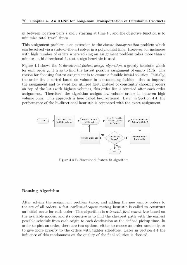
70 Chapter 4. An ALNS for Long-haul Transportation of Perishable Products
m between location pairs i and j starting at time t1, and the objective function is tominimize total travel times.
This assignment problem is an extension to the classic transportation problem whichcan be solved via a state-of-the-art solver in a polynomial time. However, for instanceswith high number of orders where solving an assignment problem takes more than 5minutes, a bi-directional fastest assign heuristic is used.
Figure 4.4 shows the bi-directional fastest assign algorithm, a greedy heuristic whichfor each order p, it tries to find the fastest possible assignment of empty RTIs. Thereason for choosing fastest assignment is to ensure a feasible initial solution. Initially,the order list is sorted based on volume in a descending fashion. But to improvethe assignment and to avoid low utilized fleet, instead of constantly choosing orderson top of the list (with highest volume), this order list is reversed after each orderassignment. Therefore, the algorithm assigns low volume orders in between highvolume ones. This approach is here called bi-directional. Later in Section 4.4, theperformance of the bi-directional heuristic is compared with the exact assignment.
Figure 4.4 Bi-directional fastest fit algorithm
Routing Algorithm
After solving the assignment problem twice, and adding the new empty orders tothe set of all orders, a fast earliest-cheapest routing heuristic is called to constructan initial route for each order. This algorithm is a breadth-first search tree based onthe available modes, and its objective is to find the cheapest path with the earliestpossible schedule from each origin to each destination at the defined pickup time. Inorder to pick an order, there are two options: either to choose an order randomly, orto give more priority to the orders with tighter schedules. Later in Section 4.4 theinfluence of this randomness on the quality of the final solution is checked.

4.3 Solution Algorithm 71
4.3.2 Neighborhoods and Operators
Now that an initial solution is available, the next step is to define efficient movesin the solution space that find improved solutions. Each move corresponds to aneighborhood. A Neighborhood of a solution z is the set of all points z′ in the solutionspace that are generated by modifying some parts of solution z [Talbi, 2009].
In the literature of FCMNFP problems, neighborhoods are grouped into thesecategories:
� node-based neighborhoods, where solutions are modified by removing or insert-ing at least one node, and the flows entering and exiting them,
� arc-based neighborhoods, where solutions are modified by removing or insertingat least one arc, and the flows passing through them,
� path-based neighborhoods, where solutions are modified by removing or insertingat least one path, and their related flows,
� cycle-based neighborhoods, where solutions are modified by removing orinserting at least one asset cycle, and their related flows.
These neighborhoods can be obtained by random or systematic moves, based on thestructure of solutions. Node-based and arc-based neighborhoods are usually small,but the other two are usually large. A neighborhood is large, when its size growsexponentially with the size of the problem.
Cycle-based neighborhoods are only applicable to solutions of problems where assetshave cyclic routes, and design-based constraints are enforced for them. For theplanning problem of Section 4.1, these neighborhoods are irrelevant. Arc-based andnode-based neighborhoods are also not well-suited for this problem. Due to tightdelivery and TTS constraints, these neighborhoods are not sufficient to escape a localoptimum, or to search larger areas of the solution space. Therefore, in this research,path-based neighborhoods are considered.
The algorithms searching for these neighborhoods are called operators. Operators canbe optimization-based or heuristic. However, if an operator is not fast, it might lose itsvalue in an ALNS algorithm. For the multimodal long-haul transportation planningproblem of this chapter, computational burdens related to the problem dimensionalityremains, and optimization-based operators are not desirable.
There are different strategies to set up and organize operators:
� like the majority of ALNS literature, define two general sets of destroy andrepair operators, where the neighborhood structure of each pair of destroy andrepair operators match well,

72 Chapter 4. An ALNS for Long-haul Transportation of Perishable Products
� categorize neighborhoods, such that operators of each category only matchothers from the same category,
� define only one set of advanced operators, each of which has its own set of movesto destroy and repair a solution.
In this research, two general sets of destroy and repair operators based on path-basedneighborhoods are created. The main decisions in Section 4.1 were identified on laden,assign, and repos flow decisions of orders, as well as selection of transportation modes.In this algorithm, the flow decisions are represented as routes Rcatp . Each route is apath for either a full order, or an empty order. These routes are easily accessed in asolution in polynomial time, therefore, order-based neighborhoods are used in orderto frame the operators of this research. In order-based neighborhoods, solutionsare modified by removing or inserting at least one order and their correspondingroutes and used transport modes. Such operators are general and match well. In thefollowings, the destroy and repair operators of ANS-1 are introduced. Later in thissection, the destroy and operators of ANS-2 are also introduced.
ANS-1 Destroy Operators
The following destroy operators are used in ANS-1 to remove the routes of orders:
� one random order (R1) operator,
� two random orders (R2r) operator,
� three random orders (R3r) operator,
� two similar orders (R2s) operator,
� three similar orders (R3s) operator
The chosen orders can be from laden, assign, repos categories, or their combination.The number of possibilities in a random category is equal to the size of order set, whilethe number of combinations in R2s and R3s categories depends on the composition ofthe order set P. In the random category, the orders are chosen randomly. However, inthe operators with similar orders, the orders are chosen based on two main similarities:their origin locations O(p) (or their destination locations D(p)) should be equal, andthe difference in their pickup times PT (p) (or their delivery time DT (p)) should beless than β time periods. The reason for introducing β is to avoid investigating ordersthat have completely different time and TTS requirements, as their chances to beconsolidated together are low.
ANS-1 Repair Operators
Repair operators used in ANS-1 are as the followings:

4.3 Solution Algorithm 73
� cheapest path (Ip) operator,
� scheduling (Is) operator,
� consolidate two orders (Ic2) operator,
� consolidate three orders (single) (Ic3s) operator,
� consolidate three orders (paired) (Ic3p) operator.
The cheapest path operator has a similar structure to the Dijkstra’ classic shortestpath algorithm, but instead of time, the cost of paths is evaluated.
The scheduling operator tries to find feasible consolidation options by putting RTIson later schedules of the used modes. For this purpose, two extra measures wereintroduced: the earliest depart time (EDm
ij ) and the latest depart time (LDmij ) of a
mode. These two values represent the feasible departure slack time for each mode.These slack times are first collected at the beginning of the improvement phase for allmodes in the fleet, and each time a new mode is added to the fleet in any iteration,its slack times are recomputed.
Finally, the consolidation operators aim to find the cheapest possible consolidationof the destroyed routes. In this regard, first a subnetwork is generated based onall the locations visited on these order routes. Then, on this subnetwork and foreach destroyed order, a set of all possible paths with the departing slack times ofthe used modes are generated. Later, path combinations of orders are compared tosearch for mutual modes and overlapping departing slack times. If such possibilitiesexist, the cheapest one among them is chosen. There is a fundamental differencebetween the consolidation of three order neighborhoods Ic3s and Ic3p. Figure 4.5gives an illustration of this difference. In a single consolidation neighborhood Ic3s,the flows of the three destroyed orders are consolidated on one particular item inthe fleet set (the mode between locations 2 and 3 for all orders), while in the pairedconsolidation neighborhood Ic3p, the flows of pairs of the orders are consolidated intwo different items in the fleet set (the mode between locations 2 and 3 for ordersone and two, and the mode between locations 3 and 7 for orders two and three).The paired consolidation was designed to exploit for more complicated consolidationoptions which none of other neighborhoods are capable of finding.
4.3.3 The First Adaptive Neighborhood Search (ANS-1)
After generating an initial solution and building the operators, the solution isimproved via two improvement blocks, namely ANS-1 and ANS-2 (Figure 4.2).Despite detailed differences, ANS-1 and ANS-2 have similar frameworks. Figure4.6 shows this framework and its components. Iteratively selecting the operators,generating new solutions, and evaluating the performance of these operators andtheir resulting improvements, are the main components.

74 Chapter 4. An ALNS for Long-haul Transportation of Perishable Products
Figure 4.5 An example of consolidation options in consolidate three order neighborhoods;left: consolidate three orders (single), right: consolidate three orders (paired)
In this framework, each operator has a weight, used in their selection process.Depending on the performance of the chosen operators, at the end of an iteration,their weights are adjusted.
After getting the initial solution, and until a stopping criterion is satisfied, thisadaptive neighborhood search runs an iteration of selecting operators, modifying thesolution, and updating the weights. In ANS-1, the stopping criterion is based on theπ number of iterations that the best found solution is not improved.
The adaptive neighborhood search starts with initiating a weight ωi,0 = 1 and ωj,0 = 1for each destroy operator i and repair operator j. At each iteration e and by looking atthe weights, one destroy and one repair operator is chosen based on a roulette wheelmechanism [Ropke and Pisinger, 2006]. Note that the destroy operator is selectedindependently of the repair operator. Assuming DOpers and ROpers are the totalnumber of destroy and repair operators in the ALNS, the roulette wheel chooses theoperators with probabilities of
Pr(i, e) = ωi,e
/DOpers∑i=1
ωi,e (4–5)
Pr(j, e) = ωj,e
/ROpers∑j=1
ωj,e (4–6)
After choosing a destroy operator i and a repair operator j, based on the neighbor-hoods of these operators (described in Section 4.3.2), Q order routes are chosen, thesolution z of iteration e is modified, and a new solution z′ is generated.
The cost F(z′) of the new solution can be computed from scratch, but it would betime consuming and unnecessary. Therefore, only cost changes ∆(Fe) related to the
Q order routes are computed. Assuming FDes(∑Qq=1 rq) to be the total cost of the Q

4.3 Solution Algorithm 75
Figure
4.6
Adapti
ve
Nei
ghb
orh
ood
Sea
rch

76 Chapter 4. An ALNS for Long-haul Transportation of Perishable Products
destroyed order routes and the removed related fleet, and FRep(∑Qq=1 rq) to be the
total cost of the Q repaired order routes and the added related fleet, F(z′) is equalto F(z) + ∆(Fe), where ∆(Fe) is defined as:
∆(Fe) = FRep(
Q∑q=1
rq)−FDes(Q∑q=1
rq) (4–7)
and its value is negative, if solution z has been improved.
In order to facilitate exploring unvisited parts of the solution space, for each repairoperator, a short-term memory (a Tabu list) is stored with a limit of min(α,
(|OZ |Q
)).
The value |OZ | is the size of the order set in a solution z, and Q is the number ofremoved orders. At each iteration, if the combination of Q orders does not exist inthe Tabu list, this combination is added and the removed order routes are repaired.Otherwise, another set of Q orders is removed. This strategy is particularly usefulwhen the size of problem increases and unvisited parts of the solution space need tobe explored.
Evaluating the performance of the chosen operators, and subsequently, updating theirweights, require an indication on how much they have improved solutions z and z?.Hence, the followings questions should be answered:
1. Was the best found solution z? improved?
2. If the first answer is No, was the current solution z improved?
3. If the second answer is No, is solution z′ feasible and accepted?
Depending on the answers, an score θ is obtained. θ is a equal to a given value θ1
if the operator i results in improving the global best solution, θ2 if it improves thecurrent solution, θ3 if the operator returns a feasible solution and accepts it, and θ4 ifthe operator reject the solution. With a score θ, at the end of iteration e, the weightsof destroy operator i and repair operator j are updated as:
ωi,e+1 = λωi,e + (1− λ)θ ×∆(fe) (4–8)
ωj,e+1 = λωj,e + (1− λ)θ ×∆(fe) (4–9)
The coefficient λ is a reaction factor which controls the reaction to the changes inthe performance of the algorithm [Ropke and Pisinger, 2006]. If it is equal to zero,the scores are not used, and if it is equal to one, the scores freely decide upon theweights, and there is no manual interference. This weighting system gives ANLSthe opportunity to intensify the search by giving the operators with higher weightsmore chance to be chosen, while it tries to diversify the search by the roulette wheelmechanism. Later in Section 4.4, the influence of this weighting method is checked.

4.4 Computational Results 77
4.3.4 Long-term Memory and the Second Adaptive Neighbor-hood Search (ANS-2)
The adaptive layer of an ANS-1 provides a good balance between diversification andintensification of the neighborhood search. Keeping a short-term memory list andtuning its parameters also help diversifying the search further, however, as the numberof orders P increases, a questions is raised on whether these strategies are sufficientin diversifying the search. Increasing the stopping criterion π to a very large number,or allowing ALNS to run for a very long time might lift this concern, but a lengthymetaheuristic is not desirable. Otherwise, optimization-based operators could havebeen introduced to the algorithm. Therefore, in the proposed algorithm of Figure 4.2,in addition to keeping short-term Tabu lists, a long-term memory is kept, trackingthe number of times each order has been chosen in all iterations of ANS-1.
Then, the set of orders is sorted based on these statistics in an ascending order, andANS-2 is executed. ANS-2 has a similar structure to Figure 4.6, but it has newdestroy operators, and some modified parameter setting, such as a stopping criterionof η = 0.5 × π, representing the number of iterations without improving the bestfound solution.
The new destroy operators of ANS-2 are as follows:
� the least chosen order (D1) operator,
� the two least chosen orders (D2l) operator,
� the three least chosen orders (D3l) operator,
� two similar least chosen orders (D2s) operator,
� three similar least chosen orders (D3s) operator.
Clearly, the first three operators pick the orders with the least number of times thatthey have been checked during all iterations of ANS-1 and ANS-2. The latter threeoperators on the other hand, try to choose the least checked similar orders. ANS-2runs with the same cheapest path, scheduling, and consolidation repair operators ofANS-1, as they match well with the new destroy operators. Later in the next section,the influence of ANS-2 on improving diversification is discussed.
4.4 Computational Results
In this section, the algorithm presented in Section 4.3 is tested on the three groups ofinstances presented in Section 3.5, with 7, 11, and 20 locations, three transportationmodes of truck, train, and barge, 12-hour, 24-hour, or 48-hour delivery service, anddifferent number of orders. The instances are named as ”nAmBtCoDE” where valueof A shows the number of locations, value of B is the number of mode types, value
78 Chapter 4. An ALNS for Long-haul Transportation of Perishable Products
of C is the planning horizon, and value of D stands for the number of orders. Theinstances with m1 only have truck options, the instances with m2 have truck andtrain options, and the instances with m3 have all modes available. If there is an orderset with tight delivery due dates, E is “t”, and if the delivery due dates are loose, Eis “l”.
In the following sections, the parameter setting are described, and the computationalresults and some sensitivity analysis are provided.
4.4.1 Parameter Tuning
Prior to showing the final results and discussing the quality of ALNS solutions, itstuning is explained. For the basic parameters, after several initial tests, the followingvalues were chosen: ALNS scoring parameters of θ1 = 30.0, θ2 = 20.0, θ3 = 10.0,θ4 = 1.0, and λ = 0.5, the time interval of β = 10 and the stopping criteria of π = 500and η = 125. Higher stopping criteria might improve the solution even further, butthe improvement compared to the time spent on the extra iterations does not seemuseful. Higher values for θ1 and θ2 also might result in getting stuck in local optimaand less diversified neighborhood search.
4.4.2 Overall Results
In this section, the results of Gurob solver in Section 3.5 are compared with the onesfrom the proposed ALNS.
Table 4.1 gives the obtained upper bounds within 10 hours. As it is shown, Gurobisolver is not able to find the optimal solution of the majority of the instances in 10hours. In the group of n20, it is almost unable to find any solutions without runningout of memory. In an extra attempt, the initial solution of ALNS was used as theMIP start solution, which only had a limited effect as it helped finding near-optimalsolutions for only two more instances n11m1o10 and n11m3o200.
In order to compare the performance of the ALNS with Gurobi solver, a 15 minutetime limit was set for both of them (Table 4.1). As shown in the table, Gurobi solver isnot able to find any solutions for 75% the instances. Moreover, among the other 25%instances, ALNS solutions have an average optimality gap of 3.9% which is acceptableconsidering the size of the problem.
Looking at the total costs in Table 4.1, an important trend seen is that by involvingtrains, and further barges, the total cost decreases by more than 50%. These resultsencourage the usage of multimodal transportation.

4.4 Computational Results 79
Table 4.1 Overall Results
Exact (10 Hours) Exact (15 min) ALNS metaheuristic (in 15 min)
n m t oUpperBound
Gap(%)
Comp.Time(sec.)
UpperBound
Gap(%)
Bestfoundtotalcost
Diff. (%)comparedto Exact10 hours
Diff. (%)comparedto Exact15 min
n7 m1 t48 o10 55167 0.00 4423 N.S. - 55167 0.00 -n7 m2 t48 o10 13786 0.00 1018 13786 3.96 14071 2.07 2.07n7 m3 t48 o10 13264 0.00 3269 N.S. - 13497 1.76 -n7 m1 t48 o25 131248 0.61 10H N.S. - 131510 0.20 -n7 m2 t48 o25 31112 0.00 4293 31123 2.84 32195 3.48 3.45n7 m3 t48 o25 30501 0.00 29219 31067 4.53 31031 1.74 -0.12n7 m1 t48 o50 249644 0.28 10H N.S. - 250672 0.41 -n7 m2 t48 o50 60992 0.00 23090 61235 2.05 62246 2.06 1.65n7 m3 t48 o50 60185 0.06 10H 60967 3.10 62042 3.09 1.76n7 m3 t48 o100 118265 0.38 10H 121818 4.41 121320 2.58 -0.41n7 m3 t48 o200 228223 0.60 10H N.S. - 236215 3.50 -
n11 m1 t48 o10 14879* 2.65 10H N.S. - 14879 0.00 -n11 m2 t48 o10 4507 0.01 5309 4507 11.66 5089 12.90 12.84n11 m3 t48 o10 3775 12.20 10H 3931 24.56 4231 12.08 7.62n11 m1 t48 o25 40827 0.73 10H 40827 0.73 41420 1.45 1.45n11 m2 t48 o25 14522 1.23 10H 14865 16.27 15807 8.85 6.33n11 m3 t48 o25 13708 0.00 19912 14023 13.97 14386 4.94 2.59n11 m1 t48 o50 81463 0.77 10H N.S. - 82450 1.21 -n11 m2 t48 o50 32185 0.00 10844 32436 11.58 34998 8.74 7.90n11 m3 t48 o50 31489 1.13 10H N.S. - 32253 2.42 -n11 m3 t48 o100 62862 2.99 10H N.S. - 65985 4.97 -n11 m3 t48 o200 122292* 3.61 10H N.S. - 135430 10.74 -
n20 m1 t72 o10t N.S. - - N.S. - 57370 - -n20 m2 t72 o10t N.S. - - N.S. - 22273 - -n20 m3 t72 o10t N.S. - - N.S. - 20976 - -n20 m1 t72 o25t N.S. - - N.S. - 147624 - -n20 m2 t72 o25t N.S. - - N.S. - 55895 - -n20 m3 t72 o25t N.S. - - N.S. - 56274 - -n20 m1 t72 o50t N.S. - - N.S. - 291816 - -n20 m2 t72 o50t N.S. - - N.S. - 108454 - -n20 m3 t72 o50t N.S. - - N.S. - 103338 - -n20 m3 t72 o100t N.S. - - N.S. - 174216 - -n20 m3 t72 o200t N.S. - - N.S. - 385521 - -
n20 m1 t72 o10l N.S. - - N.S. - 57371 - -n20 m2 t72 o10l N.S. - - N.S. - 12514 - -n20 m3 t72 o10l 10353 18.43 10H N.S. - 11724 13.24 -n20 m1 t72 o25l N.S. - - N.S. - 148426 - -n20 m2 t72 o25l 19723 18.33 10H N.S. - 21434 8.67 -n20 m3 t72 o25l 18330 16.43 10H N.S. - 18421 0.50 -n20 m1 t72 o50l N.S. - - N.S. - 289758 - -n20 m2 t72 o50l N.S. - - N.S. - 44215 - -n20 m3 t72 o50l N.S. - - N.S. - 40158 - -n20 m3 t72 o100l N.S. - - N.S. - 73893 - -n20 m3 t72 o200l N.S. - - N.S. - 178640 - -
n20 m2 t72 o1000t N.S. - - N.S. - 483754 - -n20 m3 t72 o2000t N.S. - - N.S. - 502649 - -n20 m3 t72 o1000l N.S. - - N.S. - 156344 - -n20 m3 t72 o2000l N.S. - - N.S. - 401739 - -
Note: N.S. stands for “No Solution” and 10H is an abbreviation for 10 Hour time* These results have been obtained by setting a MIP initial solution equal to the initial solution of ALNS

80 Chapter 4. An ALNS for Long-haul Transportation of Perishable Products
Table 4.2 Comparison of the Performance of ALNS with Different Repair Combinations
Sc0 Sc1 Sc2 Sc3 Sc4
n m t oAverageTotalCost
A.D.(%)
CostDiff.
A.D.(%)
CostDiff.
A.D.(%)
CostDiff.
A.D.(%)
CostDiff.
A.D.(%)
n7 m3 t48 o100 125511 0.17 -1220 0.22 -2278 0.35 -2707 0.10 -3423.92 0.50
n11 m3 t48 o10 4643 1.07 -444 0.63 -372 1.78 -439 0.91 -423 4.23n11 m2 t48 o25 17244 0.70 -1004 1.22 -1455 1.63 -1965 0 -1466 1.83n11 m3 t48 o200 145096 0.01 -3297 0.38 -4960 1.14 -4547 0.67 -7667 0.25
n20 m3 t72 o50t 108900 0.46 -5339 0.78 -4260 0.10 -4128 1.29 -3242 0.92n20 m3 t72 o100t 180420 0.19 -5631 0.33 -7633 0.53 -6222 0.54 -7576 0.35
n20 m3 t72 o10l 13889 0.80 -2117 0.61 -2058 0.19 -2071 0 -2125 0.00n20 m3 t72 o25l 21571 0 -2517 0 -2131 3.08 -3111 0.44 -2738 3.92n20 m3 t72 o200l 203215 2.27 -20080 0.06 -23839 1.35 -25510 0.90 -29209 2.13
Average - 0.63 - 0.47 - 1.13 - 0.54 - 1.57
Sc0: including repair operators Ip, IsSc1: including repair operators Ip, Is, Ic2Sc2: including repair operators Ip, Is, Ic2, Ic3pSc3: including repair operators Ip, Is, Ic2, Ic3sSc4: including repair operators Ip, Is, Ic2, Ic3p, Ic3s
4.4.3 Algorithm Performance
In this section, the efficiency of destroy and repair operators is tested based onboth the time they spend and their share of solution improvement. Furthermore,the strategies used to improve the results and reduce the computation time areinvestigated. The impact of the quality of the initial solutions on the performanceof the algorithm is also checked. Note that for the performance analysis, only nineout of 48 instances are investigated. These sample instances have an adequate varietyin number of locations and orders. For each analysis, a series of test scenarios arecompared. A test scenario corresponds to a particular ALNS setting with specific setof destroy and repair operators, scoring mechanism, initial solution constructor, anddiversification strategy.
Operator Combinations
In order to analyze the behavior of the repair (or destroy) operators, a few testscenarios with particular combination of repair (or destroy) operators are defined.The number of possible combinations is high, but the scenarios presented here areargued to give a good overview on the behavior of the operators. Operators Ip and Isare kept in all scenarios as they are fast and effective. Table 4.2 shows a comparison ofthe average total cost and the average deviations (A.D.) obtained over 10 repetitionsof ALNS. As it is shown in Table 4.2, scenario Sc4 which includes all operators, has thebest performance. Moreover, the performance of scenarios Sc2 and Sc3, especially inlarger instances, shows that the repair operators which consolidate three order routesare important contributors to the cost improvement. However, based on Table 4.3,these operators are time-consuming. This is due to the fact that the consolidationoperators need to analyze large sets of consolidation options.
In order to compare the behavior of the repair operators, all destroy operators were

4.4 Computational Results 81
Table 4.3 Comparison of the Computation Time (Seconds) of ALNS with DifferentRepair Combinations
n m t o Sc0 Sc1 Sc2 Sc3 Sc4
n7 m3 t48 o100 2.00 4.87 8.19 104.83 100.24
n11 m3 t48 o10 0.78 1.60 2.85 21.26 59.98n11 m2 t48 o25 0.84 1.23 2.72 13.89 5.60n11 m3 t48 o200 9.24 12.19 30.55 83.19 387.31
n20 m3 t72 o50t 3.63 12.25 84.41 1775.01 2723.86n20 m3 t72 o100t 8.49 33.92 202.51 1226.20 5798.21
n20 m3 t72 o10l 0.85 1.67 6.39 19.36 35.86n20 m3 t72 o25l 1.62 3.66 16.39 352.43 410.20n20 m3 t72 o200l 25.91 124.11 1196.12 2570.61 7968.14
Sc0: including repair operators Ip, IsSc1: including repair operators Ip, Is, Ic2Sc2: including repair operators Ip, Is, Ic2, Ic3pSc3: including repair operators Ip, Is, Ic2, Ic3sSc4: including repair operators Ip, Is, Ic2, Ic3p, Ic3s
Table 4.4 The Role of Destroy Operator
D1 D2r D2s D3r D3s
Extra Cost (%) including the operator only 9.92 1.83 7.93 4.81 4.10Extra Cost (%) excluding the operator 0.31 0.13 1.49 0.69 1.42
Computation Time (Seconds) 0.001 0.035 0.128 0.145 0.700
included in each scenario of Tables 4.2 and 4.3. In the followings, the efficiency ofeach destroy operator is tested. For this purpose, similar to scenario Sc4, all repairoperators are included in this test. Since the destroy operators have a similar structureand mostly the number of orders they remove is different, the scenarios with differentcombinations of these operators are not that distinct. Therefore, scenario Sc4 isrun once including each of the operators alone, and once excluding them, and it ischecked how much on average the cost of the solutions are different from the cost ofthe solution of scenario Sc4 including all of the destroy operators.
Table 4.4 shows the role of each destroy operator over 10 repetitions of ALNS. Firstof all, as shown in Table 4.4, the time these operators spend to remove a set of ordersis a matter of milliseconds. Next, the table shows that excluding each of them resultsin more expensive solutions by around 1%. It is even more expensive to use themalone. In conclusion, each destroy operator has a significant contribution to the costimprovement.
Scoring Mechanism
Depending on what moves an operator takes, and how much it modifies a solution,it can be fast or time-consuming. In order to keep the computation time of ALNSlow, the computation time of each iteration e is included into the scoring system. Ina new test scenario Sc5, the weight of operators are updated by:
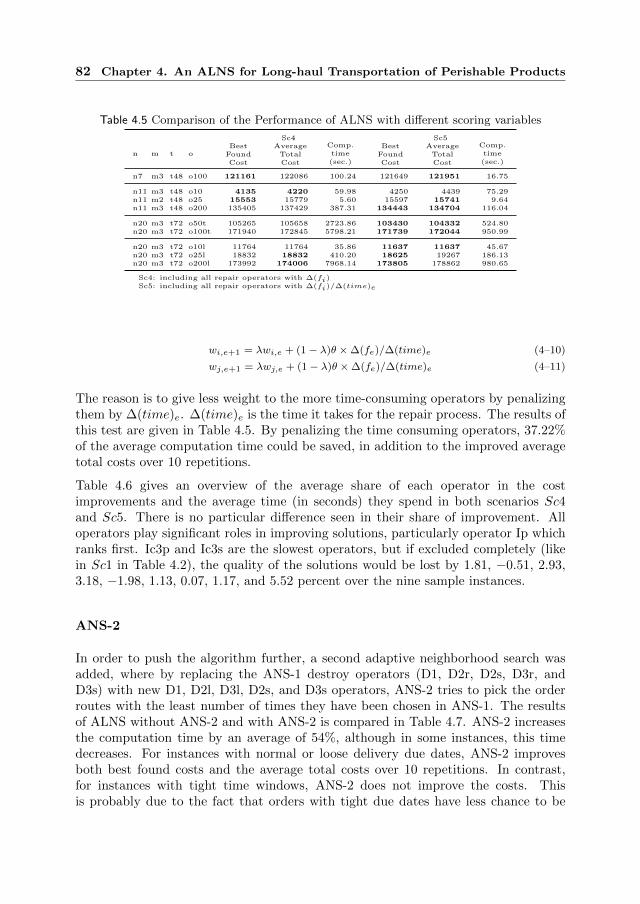
82 Chapter 4. An ALNS for Long-haul Transportation of Perishable Products
Table 4.5 Comparison of the Performance of ALNS with different scoring variables
Sc4 Sc5
n m t oBest
FoundCost
AverageTotalCost
Comp.time(sec.)
BestFoundCost
AverageTotalCost
Comp.time(sec.)
n7 m3 t48 o100 121161 122086 100.24 121649 121951 16.75
n11 m3 t48 o10 4135 4220 59.98 4250 4439 75.29n11 m2 t48 o25 15553 15779 5.60 15597 15741 9.64n11 m3 t48 o200 135405 137429 387.31 134443 134704 116.04
n20 m3 t72 o50t 105265 105658 2723.86 103430 104332 524.80n20 m3 t72 o100t 171940 172845 5798.21 171739 172044 950.99
n20 m3 t72 o10l 11764 11764 35.86 11637 11637 45.67n20 m3 t72 o25l 18832 18832 410.20 18625 19267 186.13n20 m3 t72 o200l 173992 174006 7968.14 173805 178862 980.65
Sc4: including all repair operators with ∆(fi)Sc5: including all repair operators with ∆(fi)/∆(time)e
wi,e+1 = λwi,e + (1− λ)θ ×∆(fe)/∆(time)e (4–10)
wj,e+1 = λwj,e + (1− λ)θ ×∆(fe)/∆(time)e (4–11)
The reason is to give less weight to the more time-consuming operators by penalizingthem by ∆(time)e. ∆(time)e is the time it takes for the repair process. The results ofthis test are given in Table 4.5. By penalizing the time consuming operators, 37.22%of the average computation time could be saved, in addition to the improved averagetotal costs over 10 repetitions.
Table 4.6 gives an overview of the average share of each operator in the costimprovements and the average time (in seconds) they spend in both scenarios Sc4and Sc5. There is no particular difference seen in their share of improvement. Alloperators play significant roles in improving solutions, particularly operator Ip whichranks first. Ic3p and Ic3s are the slowest operators, but if excluded completely (likein Sc1 in Table 4.2), the quality of the solutions would be lost by 1.81, −0.51, 2.93,3.18, −1.98, 1.13, 0.07, 1.17, and 5.52 percent over the nine sample instances.
ANS-2
In order to push the algorithm further, a second adaptive neighborhood search wasadded, where by replacing the ANS-1 destroy operators (D1, D2r, D2s, D3r, andD3s) with new D1, D2l, D3l, D2s, and D3s operators, ANS-2 tries to pick the orderroutes with the least number of times they have been chosen in ANS-1. The resultsof ALNS without ANS-2 and with ANS-2 is compared in Table 4.7. ANS-2 increasesthe computation time by an average of 54%, although in some instances, this timedecreases. For instances with normal or loose delivery due dates, ANS-2 improvesboth best found costs and the average total costs over 10 repetitions. In contrast,for instances with tight time windows, ANS-2 does not improve the costs. Thisis probably due to the fact that orders with tight due dates have less chance to be

4.4 Computational Results 83
Table 4.6 Comparison of the Performance of the operators
Sc4Share of improvement in total cost (%) Computation time (sec.)
n m t o Ip Is Ic2 Ic3p Ic3s Ip Is Ic2 Ic3p Ic3s
n7 m3 t48 o100 49.65 0.89 6.13 38.84 4.48 2 0 1 14 185
n11 m3 t48 o10 69.90 2.79 18.22 8.47 0.62 1 1 2 54 773n11 m2 t48 o25 49.69 1.76 4.55 22.19 21.82 1 1 2 5 12n11 m3 t48 o200 58.37 8.48 18.67 11.45 3.03 6 1 3 12 195
n20 m3 t72 o50t 47.88 1.29 11.75 27.76 11.32 8 1 3 498 7106n20 m3 t72 o100t 69.25 2.32 6.69 8.57 13.17 36 1 7 492 9649
n20 m3 t72 o10l 90.34 0.78 3.53 4.68 0.66 4 1 1 82 139n20 m3 t72 o25l 84.23 0.91 12.00 2.61 0.26 7 0 7 185 1061n20 m3 t72 o200l 71.89 1.81 14.05 2.06 10.19 7 1 7 495 7532
Sc5Share of improvement in total cost (%) Computation time (sec.)
n m t o Ip Is Ic2 Ic3p Ic3s Ip Is Ic2 Ic3p Ic3s
n7 m3 t48 o100 59.51 1.18 13.68 24.54 1.08 2 1 0 8 10
n11 m3 t48 o10 37.54 2.81 14.30 45.23 0.11 1 0 3 38 853n11 m2 t48 o25 57.50 2.92 3.88 35.62 0.08 1 1 0 6 32n11 m3 t48 o200 52.27 7.57 5.72 29.04 5.40 5 0 2 7 31
n20 m3 t72 o50t 55.91 1.76 21.71 7.98 12.64 6 0 8 89 3682n20 m3 t72 o100t 58.70 2.05 7.83 19.38 12.05 12 0 4 87 1674
n20 m3 t72 o10l 82.15 0.55 2.28 14.39 0.64 4 0 2 49 125n20 m3 t72 o25l 91.64 0.45 0.43 5.75 1.73 5 0 6 137 11n20 m3 t72 o200l 34.29 1.21 3.93 40.55 20.03 21 0 4 79 278
Sc4: including all repair operators with ∆(fi)Sc5: including all repair operators with ∆(fi)/∆(time)e
Table 4.7 Comparison of the Performance of ALNS with and without ANS-2
Sc5 Sc6
n m t oBestTotalCost
AverageTotalCost
A.D.(%)
Comp.time(sec.)
BestTotalCost
AverageTotalCost
A.D.(%)
Comp.time(sec.)
n7 m3 t48 o100 121648 121951 0.50 16.75 121212 121489 0.20 30.53
n11 m3 t48 o10 4250 4439 4.23 75.29 4137 4255 2.27 26.50n11 m2 t48 o25 15597 15741 1.83 9.64 15581 15582 0.01 8.66n11 m3 t48 o200 134442 134704 0.25 116.04 133115 134236 0.79 80.49
n20 m3 t72 o50t 103430 104332 0.92 524.80 104238 104681 0.36 719.96n20 m3 t72 o100t 171739 172044 0.35 950.99 172353 173136 0.41 0
n20 m3 t72 o10l 11637 11637 0 45.67 12041 12066 0.41 56.18n20 m3 t72 o25l 18625 19267 3.92 186.13 18124 18779 4.95 782.19n20 m3 t72 o200l 173804 178862 2.31 980.65 171704 172428 0.46 3243.35
Average - - 1.59 - - - 1.09 -
Sc6: Sc5 plus ANS-2
consolidated into slower and cheaper transportation modes. In overall, the comparisonof average deviations shows that ALNS with ANS-2 has a more robust outcome.
Quality of Initial Solutions
To test robustness of ALNS, the effect of the quality of initial solutions on thefinal obtained solutions is investigated. In Section 4.3.1, two exact and heuristicassignment algorithms were introduced for the assignment of empty RTIs in the

84 Chapter 4. An ALNS for Long-haul Transportation of Perishable Products
Table 4.8 Comparison of Exact Assignment and Heuristic Assignment
Sc6 Sc7
n m t oAverage
Initial Cost
A.D.(%)
AverageTotal Cost
A.D.(%)
AverageInitial Cost
A.D.(%)
AverageTotal Cost
A.D.(%)
n7 m3 t48 o100 291079 5.94 121489 0.20 240753 5.44 100266 0.86
n11 m3 t48 o10 9867 21.40 4255 2.27 8357 10.60 5152 0n11 m2 t48 o25 33657 9.87 15582 0.01 38064 8.51 19503 0.27n11 m3 t48 o200 254989 2.07 134236 0.79 232369 2.83 113134 1.52
n20 m3 t72 o50t 195979 8.74 104681 0.36 186076 4.59 92386 0.45n20 m3 t72 o100t 337400 1.65 173136 0.41 380021 4.10 191214 3.66n20 m3 t72 o200t 731008 2.08 385521 0.73 739022 2.50 407219 4.05
n20 m3 t72 o10l 34476 17.80 12066 0.41 24423 18.76 10316 0.75n20 m3 t72 o25l 74611 6.10 18779 4.95 64018 10.67 22647 0.44n20 m3 t72 o100l 246670 6.87 73893 4.52 1279967 4.32 77906 5.11n20 m3 t72 o200l 653806 3.59 172428 0.46 510641 5.77 189498 0.00
n20 m3 t72 o1000t N.I. - - - 766434 0.50 483754 6.10n20 m3 t72 o2000t N.I. - - - 1437041 1.01 502649 6.48n20 m3 t72 o1000l N.I. - - - 649983 1.88 156344 0.00n20 m3 t72 o2000l N.I. - - - 1216513 0.96 401739 7.09
Average - 7.82 - 1.37 - 5.50 - 2.45
N.I. stands for No obtained Initial solution in 15 minutes.Sc7: Sc6 with heuristic assignment of empty RTIs
initial solutions. It was also explained that in the heuristic assignment, orders areeither chosen randomly or prioritized based on how tight their delivery due datesare. Table 4.8 shows that for very large instances (with more than 1000 orders), astate-of-the-art solver is not able to find an initial solution in a 15 minute time limit.In contrast, ALNS with the heuristic assignment results in worse solutions in otherinstances compared to the exact algorithm. This is due to the fact that the assignmentheuristic is a greedy fastest-fit algorithm, assigning one order at a time, which is notefficient.
Summarizing remarks
To conclude this section, results show that each operator plays an important role inthe overall improvement and the algorithm shows a robust behavior. However, thetime the operators spend processing needs to be controlled. This is done by a scoringsystem depending on both cost change and CPU time consumption. In addition, theadded long-term memory and diversified search in ANS-2, provides further explorationof the solution space.
4.4.4 Incomplete Transportation Network
So far, results were based on the assumptions that the multimodal network iscomplete. In practice, not all modes are feasible for each pair of locations. Thereason to work under such an assumption was to allow each mode of transportationan equal chance, and to see their involvement without considering network boundaries.
In this section, the results are compared with a realistic TEN-T network. Figure 4.7

4.5 Conclusions 85
Figure 4.7 The horticultural network of hubs around the Europe; the white squares showthe inbound hubs, and the red circles represent the outbound hubs
gives an illustration of the rail and water connections in Europe with much fewermultimodal options for instances of n11 and n20. Still, all locations are connected byroad which is reasonable (not shown in figure).
Table 4.9 shows the huge difference between the total costs of the two cases. In theincomplete network, the costs and the number of employed trucks increase by onaverage 175% and 303% respectively. The number of trains and barges on the otherhand decrease by on average 27% and 53%.
Looking at the structure of routes in both complete and incomplete network results,it is clear that direct road connections are mostly used. However, in the incompletenetwork results, there is more variety of multimodal routes with two and threetransshipments, while in the complete network results, the number of transshipmentsis at most one and the varieties with more transshipments are rare.
4.5 Conclusions
Following Chapter 3, this chapter focused on the tactical planning problem ofperishable products with management of RTIs. Due to the complexity of this problem,a state-of-the-art MIP solver is not able to solve it for practical sizes. Therefore,in this chapter, an ALNS algorithm was proposed, which starts with constructing

86 Chapter 4. An ALNS for Long-haul Transportation of Perishable Products
Table 4.9 Comparison of the Results between Complete and Incomplete MultimodalNetwork
Complete Network Incomplete Network
n m t oAverage
Initial CostNo.
TrucksNo.
Trains
No.Barges
AverageInitial Cost
No.Trucks
No.Trains
No.Barges
n20 m3 t72 o100t 174216 108 34 47 336113 306 40 26n20 m3 t72 o200t 385521 238 55 68 808214 701 54 38n20 m3 t72 o100l 73893 51 49 56 226586 232 44 26n20 m3 t72 o200l 178640 142 65 84 545628 504 60 30
n20 m3 t72 o1000t 483754 266 132 125 772169 693 74 79n20 m3 t72 o2000t 502649 519 216 215 1518313 1307 84 96n20 m3 t72 o1000l 156344 81 137 141 613086 616 75 57n20 m3 t72 o2000l 401739 220 277 295 1327066 1245 95 82
an initial solution, and tries to improve this solution by iteratively exploring largeneighborhoods. New path-based neighborhoods and their associated destroy andrepair operators were introduced in this ALNS. These operators work on variouscombination of order routes.
The proposed ALNS contains two blocks of adaptive neighborhood search heuristics,where systematically choose a destroy and a repair operator to modify solutionsand find improvements. These operators have selection weights, and depending onhow well they perform, a scoring mechanism updates their weights. Therefore, well-performing operators get higher chances of being reselected. A modified scoring is usedin this chapter, where not only solution quality is checked, but also the computationtime of operators are considered.
The proposed ALNS uses a short-term Tabu search to add more diversification to itssearch and prevent redundancies, but a long-term memory was also added to exploitunvisited parts of the solution space by looking at the neighborhoods of the orderroutes that have not been investigated often.
The proposed algorithm is fast, does not take up much memory, and provides goodsolutions. It is even able to find solutions for the instances that a state-of-the-art MIPsolver cannot find any solution for. The only weakness of the proposed algorithm is inits assignment heuristic. In instances with less than 1000 orders, this heuristic resultsin more expensive solution, compared to when its assignment problem is solved by astate-of-the-art MIP solver.
Possible future work can be to improve the assignment heuristic, for instance byadding an iterative local search to improve the obtained assignment. The proposedALNS in this chapter was designed to solve a tactical planning level problem. Anotherextension is to study the operational planning level problem, where this assumptionis relaxed that the information on all coming orders is available, and the solutionalgorithm responds to day-to-day changes and new demand. This is the subject ofChapters 5 and 6.

Part III
Operational Planning


Chapter 5
A Rolling Horizon Frameworkfor Operational Planning ofLong-haul Transportation ofPerishable Product
The multimodal long-haul transportation planning problems studied in this thesisare grouped into tactical and operational planning problems. In Chapters 3 and4, the tactical planning problems were described and modeled, and a metaheuristicalgorithm to solve practical sizes was proposed. Tactical planning problems see theworld as static, while in practice, the world is constantly evolving. Operationalplanning problems on the other hand, assume the world to be dynamic, and aimto optimally respond to the system changes and new information. The currentchapter aims to frame the operational planning problem of long-haul transportationof perishable products, its structure, and elements. Section 5.1 starts with describingthis problem. Section 5.2 gives an overview on the relevant literature, and Section 5.4explains the proposed rolling horizon framework, its properties, and essential settings.In Section 5.5, a comprehensive computational analysis is presented, and finally, inSection 5.6, some concluding remarks are provided.
5.1 Problem Description
On the operational floor of a transportation system, hundreds of loaded and emptyunits and items are handled and moved on sight, and the people sitting in thecontrol tower are constantly observing dynamics of the operations and outside world,

90 Chapter 5. A Rolling Horizon Framework for Operational Planning
receiving new customer demands, comparing practice with the plans on paper, andmaking decisions in response to these changes. For this purpose, companies useDecision Support Systems or Softwares (DSS), where they can monitor and controlthe evolution of operations, collect and analyze data, make new decisions, and finallyexecute the relevant plans. Operational planning problems are defined at the heartof such DSS’s.
One might argue that operational plans are not needed and tactical plans are sufficientfor execution. The problem is that tactical plans are fixed and based on aggregate dataand estimations, they can only provide an overall perspective even if they include somelevel of uncertainty in the planning. The operational planning problem of long-haultransportation of perishable products is non-stationary, meaning that there mightbe days that customer demands are more volatile than expected, and a fixed flowand repositioning plan might not fully and efficiently fulfill them [Sethi and Sorger,1991]. For instance, if demands are much higher than expected, in order to satisfycustomer requirements, last-minute expensive fleet options are employed. On theother hand, if demand is much less than expected, the a priori planned fleet mightbecome underutilized, which is again costly. Operational planning problems are thendefined to include decisions on needed flexibility while ensuring efficiency.
In order to understand the operational planning, its decisions and objectives, first,it is important to understand its structural differences to the tactical planningproblems. Similar to tactical planning, operational planning deals with utilizinga given transportation infrastructure by choosing the best services and associatedmodes, efficient allocation of their capacities to customer demands, and managementof all resources involved. However, in operational planning,
� the time interval between each two consecutive decision making occasions,
� and the planning horizon these decisions are made for,
are shorter. For instance, if in tactical planning, decisions are made at the beginningof each month to plan the operations of the coming month, in operational planning,decisions are made at the beginning of each day to plan the operations of the next72 hours. Therefore, at each decision making occasion, there are plans from previousoccasions that have not been executed yet. For instance, a truck has been planned tobe called tomorrow, but it will be reconsidered in the operational planning problemof today in case there are better consolidation options and cheaper modes.
The length of time intervals depends on how fast a system evolves, and how frequentnew decisions should be made. For instance, in distributing perishable products insidea city where the traffic constantly changes, the time intervals are close to real-time,while in long-haul transportation of perishable products where some transportationmodes have fixed routes and timetables, the length of time intervals is a matter ofhours or days. The length of planning horizons on the other hand, depends on how farand how detailed the information needed for making new decisions are accessible. For

5.1 Problem Description 91
instance, in long-haul transportation of perishable products, if the revealed customerorders should all be delivered by 72 hours, and the information on availability oftransportation modes and their schedules for the coming week is at hand, the lengthof planning horizon is set to 72 hours or a week.
Now, assuming 1) the data collection method and the decision moments given, 2) thecurrent decision making occasion is not the initial one (or in other words, this is notthe first decision making occasion), and 3) assuming to have access to the operationalplans and state of the system from previous decision making occasions, the maindecisions of the operational planning problem are as the followings:
� flow of new products (new customer demand),
� new and updated repositioning of Returnable Transport Items (RTIs),
� new and updated selection of transport modes and schedules to do these jobs.
Similar to the previous chapters, the main decisions are defined on RTI flow,repositioning, handling, and holding throughout the network and over the givenplanning horizon. Then, the role of updated decisions in a particular planning horizonis to look for opportunities to consolidate new RTI flows with the old ones.
Demand is represented by orders. Orders arrive to the system at different time periodsof a time interval, and future orders of future intervals are unknown. An order ischaracterized by its pair of origin and destination locations, its volume, its pickupand delivery schedules, and its freshness requirements. Since RTIs are the loadingunits used to transport the products, the order volume shows the number of RTIs(e.g. 2 trolleys) needed to transport products from the origin to the destination. Theproducts can be picked up and loaded onto the RTIs at an earliest given time, andshould be delivered to the destination and unloaded at an latest given time. Theseschedules are not definite though, and as long as the order is transported within thelength of this schedule, its flow is feasible. For instance, an order might be held fora few hours at its origin destination before it is loaded and transported. Similar toChapter 3, product freshness is approximated by a Time Temperature Sum (TTS)measure, and a maximum limit is enforced on the TTS of orders.
In order to transport RTIs over the given planning horizon, fleets of differenttransportation modes over the coming planning horizon are assumed availablethroughout the network. Each transport mode has its given schedules, and its vehiclesoperate based on them. Each mode has a specific temperature, showing for examplethe temperature inside a truck trailer, a train car, or a barge storage room. Also,the vehicles are capacitated, and there are limited number of vehicles available foreach transport modes. In comparison to tactical planning problem however, thecharacteristics of available fleet is dynamic, and from one time interval to the next,might be different.
The objective function of operational planning problems can also be dynamic, ifcosts of available transportation modes and services change over different planning
92 Chapter 5. A Rolling Horizon Framework for Operational Planning
horizons. For instance, it might be cheaper to rent a truck tomorrow than to rent ittoday. Moreover, depending on how much operations are based on a priori fixed plans,an objective function of operational planning problems can have different forms. Ifoperations have no fixed plans, the objective function can have a form similar toa tactical counterpart but with dynamic costs, but if there are fixed plans, theremight be defined penalties on how much operations deviates from these plans, andthe objective is to minimize the deviations. For example, in case a reserved trainservice is canceled, a cancellation charge should be paid. In this chapter, the objectivefunction is to minimize total operational costs, including flow costs of the loaded RTIs,flow costs of the assigned and repositioned empty RTIs, locational costs, and finally,costs of using the modes, over all rolled planning horizons. Note that there is nocancellation or change of path for the moving vehicles on their routes.
5.2 Related Literature
Operational planning problems in the transportation planning literature, dependingon how and when data is collected and decisions are made, are referred to as dynamic,real-time, or online planning problems. Moreover, depending on whether uncertaintyof future events and their anticipation is included, they are divided into deterministicand stochastic planning problems. The decisions in this chapter are made only basedon the known information on customer demand and system evolution, therefore, thissection only reviews literature of deterministic planning problems.
There is a vast literature on studying these classes of problems for distributionplanning, modeled as Vehicle Routing Problems (VRPs) . Ghiani et al. [2003], Larsenet al. [2008], Gendreau et al. [2015] give an overview on the recent dynamic and real-time VRPs. In dynamic VRPs, Chen et al. [2006] and Schonberger [2010] proposerolling horizon frameworks for their dynamic vehicle dispatching problems, where atcertain decision occasions, their vehicle routes are re-optimized based on new revealedcustomer demands. Yang et al. [2004] is another example of using rolling horizonapproach for a dynamic truckload pickup and delivery problem. Yang et al. [2004] useddifferent policies, either with complete re-optimization or simple heuristic updating,and show that re-optimization outperforms other policies. Mitrovic-Minic et al. [2004]also study a dynamic pickup and delivery problem with time windows and embedshort-term and long-term planning policies into their rolling horizon algorithm. Inall these examples, the decision timing and the time intervals are fixed, and decisionsare made at the given time occasions. In comparison, in real-time or online VRPs,decision timing and time intervals are not fixed, time is modeled continuous, anddecisions are made where an event (such as arrival of a new customer order, or anetwork disruption) happens. Gendreau et al. [2006] study a real-time pickup anddelivery problem where customer demands come in real-time. They propose a TabuSearch (TS) heuristic with neighborhoods based on ejection chains to insert the newcustomer demand into their plans. Hong [2012] also study a real-time VRP with

5.2 Related Literature 93
hard time windows where customer demand come in real-time. They propose aLarge Neighborhood Search (LNS) algorithm to insert the new customer demand.Li et al. [2009] on the other hand, study a real-time pickup and delivery problemwith service disruption (e.g. vehicle breakdown), where they reroute the vehiclesin real-time. They propose a Lagrangian relaxation based heuristic. A dynamicprogramming based algorithm heuristically solves the shortest path problems withresource constraints that result from the Lagrangian relaxation.
On dynamic or real-time long-haul transportation planning literature, where theproblem is deterministic, Choong et al. [2002] present a Mixed-Integer Program(MIP) for a real-world empty container management system, and analyze theeffect of length of the planning horizon on the quality of distribution plans andtheir outsourcing. They show that in general, a rolling horizon results in betteroutsourcing and distribution plans, and more usage of cheaper transportationmodes. Erera et al. [2005] present a MIP for the operational planning of amultimodal tank container where they integrate planning the repositioning ofcontainers with their routing. Then, they run the model on daily or weekly rollinghorizon framework, implementing different repositioning strategies, namely, weeklyrepositioning, bounded daily repositioning, and unbounded daily repositioning. Theyshow that daily repositioning is more advantageous than a weekly repositioning.Bandeira et al. [2009] model an integrated empty and loaded container transshipmentsystem and propose a decision support system that for each time period, it firstgenerates empty container orders, solves a static minimum cost MIP, and dynamicallyupdates and controls the obtained plans over the following planning time periods.Nielsen et al. [2012] study the real-time disruption of railway transportation, andpropose a rolling horizon approach which only considers the information of certaintime horizons in train rescheduling. They present several computational analysesincluding the relation between the solution quality and the length of the horizons.Rakke et al. [2011] model an annual planning inventory routing of liquefied naturalgas as a MIP. The problem size is too big, therefore, they solve its sub-problemsvia a rolling horizon heuristic. In their approach and at each horizon, they usesome simplified forecasts about the future periods, and while fixing the solution ofprevious periods, they solve the sub-problem of that horizon. Bock [2010] introducesa real-time-oriented control approach for efficient consolidation and transshipmentand dynamic handling of disturbances such as vehicle breakdown and accidents. Heuses rolling horizon approach where some decisions are fixed and the plans for newtime intervals are simulated. Bock [2010] designs a metaheuristic algorithm based ona Variable Neighborhood Search (VNS) which applies dynamic neighborhood searchfor generating new plans. Ahmt et al. [2015] present a MIP model and several validinequalities for a container positioning at a terminal and then solve the large instancesof this problem with a rolling horizon based heuristic. Cordeau et al. [2015] embeda routing problem with heterogeneous fleet into a rolling horizon algorithm in orderto incorporate the dynamics of new requests and the loading capacity of the fleet. Inthis algorithm, on a rolling horizon, a heuristic is used to select vehicles, an Iterative
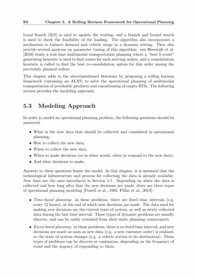
94 Chapter 5. A Rolling Horizon Framework for Operational Planning
Local Search (ILS) is used to update the routing, and a branch and bound searchis used to check the feasibility of the loading. The algorithm also incorporates amechanism to balance demand and vehicle usage in a dynamic setting. They alsoprovide several analyses on parameter tuning of this algorithm. van Heeswijk et al.[2016] study a real-time multimodal transportation planning where a “best k-route”generating heuristic is used to find routes for each arriving orders, and a consolidationheuristic is called to find the best re-consolidation option for this order among thepreviously planned orders.
This chapter adds to the abovementioned literature by proposing a rolling horizonframework containing an ALNS, to solve the operational planning of multimodaltransportation of perishable products and repositioning of empty RTIs. The followingsection provides the modeling approach.
5.3 Modeling Approach
In order to model an operational planning problem, the following questions should beanswered:
� What is the new data that should be collected and considered in operationalplanning,
� How to collect the new data,
� When to collect the new data,
� When to make decisions (or in other words, when to respond to the new data),
� And what decisions to make.
Answers to these questions frame the model. In this chapter, it is assumed that thetechnological infrastructure and process for collecting the data is already available.New data are the ones introduced in Section 5.1. Depending on when the data iscollected and how long after that the new decisions are made, there are three typesof operational planning modeling [Powell et al., 1995, Pillac et al., 2013]:
� Time-based planning : in these problems, there are fixed time intervals (e.g.every 12 hours), at the end of which new decisions are made. The data used formaking new decisions are the current state of system, as well as newly collecteddata during the last time interval. These types of dynamic problems are usuallydiscrete, and can be easily extended from their static planning counterparts.
� Event-based planning : in these problems, there is no fixed time interval, and newdecisions are made as soon as new data (e.g. a new customer order) is realized,or the state of system changes (e.g. a vehicle arrives to its destination). Thesetypes of problems can be discrete or continuous, depending on the frequency ofevent and the urgency of responding to them.

5.3 Modeling Approach 95
� Real-time planning : in these problems, decisions are continuously made. Iftime-based problems have very short time intervals, they can be defined asreal-time planning problems. Event-based problems also can become real-time,if they receive new data in very high frequencies. These planning problemsrequire a good real-time supporting technology (e.g. RFID technology, onlinetelecommunication and tracking), and their plans should be practically feasible(e.g. modes have flexible routes), otherwise, classifying an operational planningas real-time is not wise.
The Operational planning problem of this chapter belongs to the time-based planningclass. Customer orders arrive in different hours of the day, and their deliveryrequirements span over several hours (and even days). Moreover, in multimodaltransportation, where some modes have fixed timetables or routes, the moment theystart their operation, they cannot change their route or schedules. As a result,continuous type of modeling does not bring any significant value to operationalplanning of multimodal transportation. Of course, their operation might beunexpectedly disrupted, but disruptions are not exclusively considered in this chapter,and the available modes and services, which can be different from one time intervalto the next, are assumed reliable.
In time-based planning, a reoptimization method periodically solves a static problemcorresponding to the current data and system state [Pillac et al., 2013]. Thisreoptimization problem can be limited or complete. A limited reoptimization is usedwhere limited changes to the state of system are allowed or desired. For instance inevent-based planning, when a new customer order arrives, the reoptimization problemcan be formulated to find the cheapest transportation option for that order only,and the rest of orders are not included in the reoptimization problem. In contrast,a complete reoptimization problem includes all customer orders and is allowed tochange all parts of the system state, as long as they are not fixed (e.g. the vehicleshave not started their transport). In long-haul transportation of perishable products,consolidation is the key factor in decreasing operational costs, therefore, in thischapter, a complete reoptimization setup is used.
The advantage of using periodic reoptimization is that its solution algorithm canbe based on the ones developed for static problems. The operational planningproblem of long-haul transportation of perishable products with RTI managementis an extension to the Fixed-charge Capacitated Multicommodity Network FlowProblems (FCMNFP). There are many papers in this literature proposing modelsand algorithms which could be extended and embedded in a periodic reoptimizationframework. Examples can be found in Chapter 2.
The optimization problem that is periodically solved, has an infinite planning horizonin nature, meaning that there is no ending time period or ending system state to bereached. In the operational planning problem of this chapter however, customerorders that are revealed over the last time interval, have delivery deadlines, andthey all need to be delivered by the latest delivery deadline among them (e.g. 72

96 Chapter 5. A Rolling Horizon Framework for Operational Planning
Figure 5.1 Rolling horizon framework
hours). Repositioning operations also do not take more than a few hours or a fewdays. In addition, the data on available transportation modes over a long horizonis not accessible, and if accessible, they are not useful. Transportation companiesand logistics service providers usually reveal their available capacity and price until acertain time in the future (e.g. only for the next three months), and since all revealedorders and all repositioning jobs are comparably done within a shorter period (e.g.two weeks), there is no need to stretch the planning horizon farther. As a result,the infinite optimization problem is truncated into a smaller planning problem witha finite and short planning horizon T , which is rolled after a certain time interval ofτ (e.g. after every 12 hours). τ hence denotes the length of a roll.
This approach is called rolling horizon approach. Rolling horizon approaches are veryuseful in handling large-scale or dynamic problems. The only drawback of using arolling horizon framework is the possibility of ending up with suboptimal solutions.In this research, since the size of problem and the amount of details in practice ishuge, finding a good solution in reasonable time is much more important than findingthe optimal solution.
In this rolling horizon approach, at the end of a roll φ, the process of collecting newdata is stopped, and then a reoptimization problem with time periods t = φ, φ +1, . . . , φ+ T is solved (by either an exact or heuristic algorithm) to derive new plansand adjustments for the following horizon of T (Figure 5.1). Then, the new plans areexecuted until the end of roll φ+ 1. The collected data includes the set of new ordersarrived during roll φ, as well as the state of the system and resource availability bythe end of roll φ.
The periodically solved reoptimization problem is a roll-dependent version of theplanning problem of Chapter 3. Similar to that chapter, the physical transportationnetwork is characterized by i = 1, . . . ,N hub locations, and arcs (i, j) representingdifferent routes connecting these locations. Between each location pair, at least one

5.4 Rolling Horizon Framework 97
transportation mode m can operate. Each of these modes has its own capacity,maximum number of available vehicles per time period, speed, temperature, fixedcost per hour, fixed costs per vehicle, and variable costs per RTI per hour. However,these parameters might differ from one roll φ to the next. The locations also havetheir own operation time, temperature, and holding cost per RTI per hour, which canagain be roll-dependent. Locations are assumed to be uncapacitated regarding thenumber of operations they can do, the number of RTIs they can hold, or the numberof vehicles they can accommodate.
An order coming to the system during roll φ, is characterized by the number ofRTIs needed to load and transport products from an origin location to a destinationlocation. Each order has an earliest pickup time which is later than or equal tot = φ, a latest delivery due date, and a Time Temperature Sum (TTS) measure whichrepresents the total time that products can be transported in different temperatureregimes.
The length of the planning horizon T is now set to be equal to the latest delivery duedate among all collected orders of roll φ.
The objective function of the truncated problem is then to minimize total operationalcosts, including flow costs of the loaded RTIs, flow costs of the assigned andrepositioned empty RTIs, locational costs, and finally, costs of using the modes, overthe planning horizon T .
In the next section, the rolling horizon framework of this chapter is explained in detail.
5.4 Rolling Horizon Framework
Chapter 3 presented a MIP for multimodal transportation planning problem ofperishable products and RTI repositioning, and Chapter 4 introduced an AdaptiveLarge Neighborhood Search (ALNS) Algorithm to solve it.
In this chapter, the same MIP is embedded in the proposed rolling horizon framework,and the same ALNS is used to solve this MIP. The algorithm is fast and in less than acomputational time of 15 minutes, it can provide good quality solutions for instanceswith around 2000 orders.
In this section, the structure of this framework is described in detail. First, thestate of system and a solution of the reoptimization problem are defined. Then, thereoptimization process by the ALNS is explained, and finally, some updating strategiesare proposed.

98 Chapter 5. A Rolling Horizon Framework for Operational Planning
5.4.1 State of System and Roll Solution
First, it is necessary to have a clear picture of what the state of system is, to laterexplain how this state evolves and is updated. The state of system is defined by thestate of different parts of the solution at the end of roll φ. Similar to Chapter 4, asolution in this framework contains:
� a set of orders, to keep track of planned, unplanned, and newly arrived orders.An order at the end of roll φ has one of these states: new, not planned, andplanned. The orders with either of the first two states have not been planned.However, some orders have been revealed in earlier rolls but due to somecircumstances such as shortage of empty RTIs, have not been planned and werepushed forward to roll φ. If the deadline of such orders is passed, they becomelost sale.
� a set of RTI positions, with location, availability time, and volume. It is similarto the inventory concept indicating at which time period, how many RTI areavailable at a location. This set is then used for assigning empty RTIs to orders,when needed. If empty RTIs need to be repositioned, empty orders are generatedand added to the set of all orders.
� a set of routes, representing the scheduled flow of (loaded or empty) RTIs.When an order is planned, a route is generated for it. Therefore, the set ofroutes represents only planned orders. A route at the end of roll φ has also itsown states: not started, on-route to the destination, on route to a transshipment,and completed. A route does not start until its planned depart time fits in rollφ. If a route starts, its state changes to on-route. However, depending onwhether the next location on the route is the destination or a transshipmentlocation, its state is different. From planning point of view this is importantbecause the routes that have started moving RTIs, but are not on their way tothe destination location, can also be considered in the replanning strategy ofthis framework. A route that has an on-route to the destination state is notincluded in the replanning. Finally, a route is complete when the RTIs arriveto the destination location during during roll φ.
� a set of fleets, where each member represents the mode used for moving theseflows. A member fleet can have either of these states: used or unused. The usedfleet are the ones transporting RTIs on the routes with on-route states. Theothers are the fleet that have been included in the plans but their departingtime is not in roll φ. Unused fleet are incorporated in the replanning strategy,to find future consolidation options.
The state of system as described above is placed in a roll solution. A roll solution zφis the solution of roll φ, and depending on the adjustments and changes, it transformsinto a different solution zφ+1 for roll φ + 1. When a route of a planned order is

5.4 Rolling Horizon Framework 99
Figure 5.2 An overview of the data flow in a roll, based on orders
completed, the order and its route are removed, but its statistics are kept in thehistory. Likewise, if a vehicle in the fleet has arrived to its destination in roll φ, it willbe removed from the solution and only its statistics are kept. Removal of these partsprevents useless occupation of memory and extra solution search efforts. Figure 5.2gives an overview of the data flow in each roll φ.
A roll solution is then given to the MIP of Chapter 3, which has now roll-dependentright-hand side values and cost coefficients. This problem is still too complex to besolved by a state-of-the-art MIP solver. Therefore, a heuristic algorithm such as theproposed ALNS of Chapter 4 is needed to solve it.
5.4.2 ALNS and Planning Process
Figure 5.3 shows the planning process of the rolling horizon framework. Based on thestate of system or the roll solution and new data revealed during roll φ, at the end ofthe roll, the ALNS is employed to reoptimize and update the roll solution zφ. Chapter4 presents a complete description and a comprehensive computational analysis on theperformance of the ALNS used here.
Since this is a complete reoptimization process, at first, all parts of the roll solution φthat are not fixed and have not been executed yet, are destroyed. The destroyed partsinclude routes, repositioning orders, and some of the fleets that were not reservedor called yet. Then, the related orders that should be replanned are added to therevealed new orders, the list of all available transportation modes are collected, andthe position of all RTIs around the network is recorded. Afterwards, a new initial
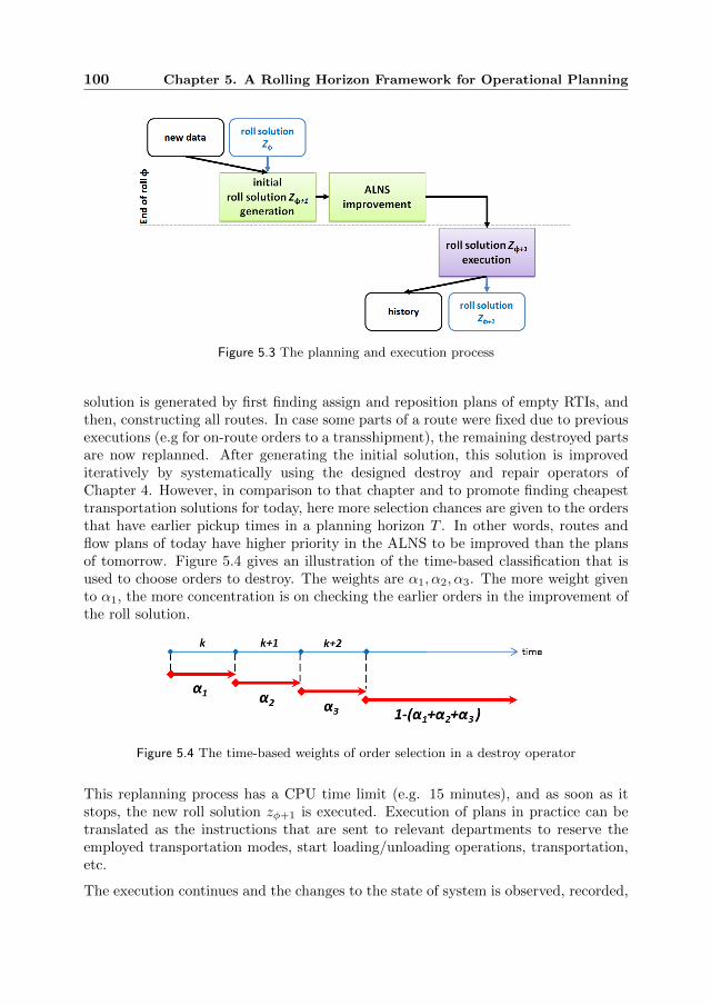
100 Chapter 5. A Rolling Horizon Framework for Operational Planning
Figure 5.3 The planning and execution process
solution is generated by first finding assign and reposition plans of empty RTIs, andthen, constructing all routes. In case some parts of a route were fixed due to previousexecutions (e.g for on-route orders to a transshipment), the remaining destroyed partsare now replanned. After generating the initial solution, this solution is improvediteratively by systematically using the designed destroy and repair operators ofChapter 4. However, in comparison to that chapter and to promote finding cheapesttransportation solutions for today, here more selection chances are given to the ordersthat have earlier pickup times in a planning horizon T . In other words, routes andflow plans of today have higher priority in the ALNS to be improved than the plansof tomorrow. Figure 5.4 gives an illustration of the time-based classification that isused to choose orders to destroy. The weights are α1, α2, α3. The more weight givento α1, the more concentration is on checking the earlier orders in the improvement ofthe roll solution.
Figure 5.4 The time-based weights of order selection in a destroy operator
This replanning process has a CPU time limit (e.g. 15 minutes), and as soon as itstops, the new roll solution zφ+1 is executed. Execution of plans in practice can betranslated as the instructions that are sent to relevant departments to reserve theemployed transportation modes, start loading/unloading operations, transportation,etc.
The execution continues and the changes to the state of system is observed, recorded,

5.5 Computational Results 101
and updated, until the next round of planning at the end of roll φ + 1, where theupdated roll solution zφ+1 is again reoptimized, considering the new data revealedduring roll φ+ 1.
5.5 Computational Results
In this section, the computational results are presented, and the sensitivity of solutionsto different rolling horizon settings and policies is tested.
The setup of the test sets and their inputs are similar to Chapter 4. The instancesare categorized in three groups of 7, 11, and 20 hub locations, where the first grouponly includes the hubs in the Netherlands, the second group includes the hubs in theBeNeLux region, and the third group includes all hubs. There are three classes oftruck, train, and barge transportation modes and truck connections are assumed tobe available between all pairs of locations, which is reasonable. However, that is notthe case for trains and barges. Figure 4.7 in Chapter 4 gives an illustration of thereal-world rail and water connections between each pair of locations in the network.Out of 20 hub locations, two are inbound hubs where the products come from allaround the world to get sold, sorted, and consolidated for the shipments.
The storage locations of empty RTIs are assumed to be in these inbound hubs, and itis required that a certain number Si(≥ 0) of empty RTIs (e.g. 5000 trolleys) shouldbe available at these locations at beginning of each week.
In order to have an real-time order arrival setup, the order set of previous chaptershave been split into orders with smaller volumes, dispersed throughout the entire year,in hourly basis. To keep the computations manageable and the length of this chapterreasonable, the whole year is not investigated though. A season was chosen and itwas divided into three instances recognized by month = 1, 2, 3. It is argued that thechosen instances represent enough variety to guarantee the generality of the analysis,especially due to their day-to-day and weekly variations indicated in Chapter 1.
All settings and parameters of the ALNS engine in this chapter have been tunedsimilar to those presented in Chapter 4. However, α1, α2, and α3 are set to 0.6, 0.2,and 0.1 respectively. Moreover, a maximum CPU time limit of 15 minutes is set asthe stopping criterion of the ALNS in each roll.
In the reminder of this section, first overall results are provided, then variousinvestigation on the sensitivity of solutions to different parameter settings is tested.Moreover, the results of complete reoptimization and partial reoptimization arecompared. Note that in most of the analysis, τ is set to 12. The reason is thatin practice, plans are updated every 12 hours.
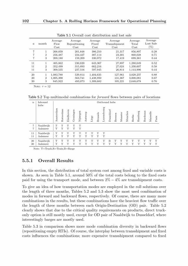
102 Chapter 5. A Rolling Horizon Framework for Operational Planning
Table 5.1 Overall cost distribution and lost sale
n monthAverage
FlowCost
AverageRepositioning
Cost
AverageFixedCost
AverageTransshipment
Cost
AverageTotalCost
AverageLost Sale
(%)
7 1 268,839 201,848 386,210 21,317 856,897 0.287 2 256,487 224,427 387,114 23,301 868,028 0.717 3 209,180 159,209 330,972 17,419 699,361 0.44
11 1 405,862 230,820 643,367 27,897 1,280,049 0.5211 2 352,499 315,893 662,216 27,024 1,330,607 0.5811 3 309,535 237,516 597,945 26,814 1,144,996 0.44
20 1 1,083,788 539,814 1,404,635 127,961 3,028,237 0.8820 2 1,005,390 563,741 1,438,950 131,367 3,008,081 0.6720 3 845,922 493,073 1,309,682 105,221 2,648,678 0.76
Note: τ = 12
Table 5.2 Top multimodal combinations for forward flows between pairs of locations
n Inboundhubs
Outbound hubs
Am
ster
dam
Rott
erd
am
Ein
dh
oven
Gro
nin
gen
Nij
meg
en
Antw
erp
Lie
ge
Bru
ssel
s
Lu
xem
bou
rg
Du
ssel
dorf
Bre
men
Mu
nst
er
Mu
nch
en
Ber
lin
Ham
bu
rg
Bord
eau
x
Mars
eille
Pari
s
7 Naaldwijk T T T T T7 Aalsmeer T T T T T
11 Naaldwijk T T T T T T T T T11 Aalsmeer T T T T T T T T T
20 Naaldwijk T T T T T T T T T B T T T T T T T T20 Aalsmeer T T T T T T T T T T T T T T T T T T
Note: T=Truck,R=Train,B=Barge
5.5.1 Overall Results
In this section, the distribution of total system cost among fixed and variable costs isshown. As seen in Table 5.1, around 50% of the total costs belong to the fixed costspaid for using the transport mode, and between 2%− 4% are transshipment costs.
To give an idea of how transportation modes are employed in the roll solutions overthe length of three months, Tables 5.2 and 5.3 show the most used combination ofmodes in forward and backward flows, respectively. Of course, there are many morecombinations in the results, but these combinations have the heaviest flow traffic overthe length of three months between each Origin-Destination (OD) pair. Table 5.2clearly shows that due to the critical quality requirements on products, direct truck-only option is still mostly used, except for OD pair of Naaldwijk to Dusseldorf, whereinterestingly barges are mostly used.
Table 5.3 in comparison shows more mode combination diversity in backward flows(repositioning empty RTIs). Of course, the interplay between transshipment and fixedcosts influences the combinations; more expensive transshipment compared to fixed
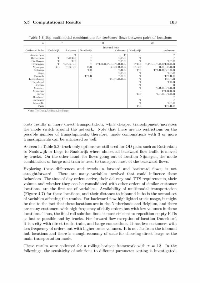
5.5 Computational Results 103
Table 5.3 Top multimodal combinations for backward flows between pairs of locations
n 7 11 20
Inbound hubsOutbound hubs Naaldwijk Aalsmeer Naaldwijk Aalsmeer Naaldwijk Aalsmeer
Amsterdam - T - T - TRotterdam T T-R,T-B T T,T-R T TEindhoven T T-R T T,T-R T T,T-RGroningen T T,T-B-R-B T T,T-R-R,T-R-B,T-R-B-B T,T-R T,T-R-B,T-R-R,T-R-B-BNijmegen B-R T,B-R-B B-R B-R-R,B-R-B T,B-R B-R-R,B-R-BAntwerp T,B T,B-B T,B T,T-R-R,B-R,B-B
Liege T T,T-R T T,T-RBrussels T,T-R T-R-R T T,T-R-R
Luxembourg T T-B,T-R-R-B T T-R,T-BDusseldorf T T,B-B
Bremen T BMunster T T-B-R-B,T-R-B
Munchen - T,T-R-R-BBerlin T-R T,T-R-R,T-B-B
Hamburg - TBordeaux T TMarseille T T,T-R
Paris T,B T,T-R-R
Note: T=Truck,R=Train,B=Barge
costs results in more direct transportation, while cheaper transshipment increasesthe mode switch around the network. Note that there are no restrictions on thepossible number of transshipments, therefore, mode combinations with 3 or moretransshipments can be witnessed as well.
As seen in Table 5.3, truck-only options are still used for OD pairs such as Rotterdamto Naaldwijk or Liege to Naaldwijk where almost all backward flow traffic is movedby trucks. On the other hand, for flows going out of location Nijmegen, the modecombination of barge and train is used to transport most of the backward flows.
Exploring these differences and trends in forward and backward flows, is notstraightforward. There are many variables involved that could influence thesebehaviors. The time of day orders arrive, their delivery and TTS requirements, theirvolume and whether they can be consolidated with other orders of similar customerlocations, are the first set of variables. Availability of multimodal transportation(Figure 4.7) for these locations, and their distance to inbound hubs is the second setof variables affecting the results. For backward flow highlighted truck usage, it mightbe due to the fact that these locations are in the Netherlands and Belgium, and thereare many customers with high frequency of daily orders but with low volumes in theselocations. Thus, the final roll solution finds it most efficient to reposition empty RTIsas fast as possible and by trucks. For forward flow exception of location Dusseldorf,it is a city with direct truck, train, and barge connections. It has less customers withless frequency of orders but with higher order volumes. It is not far from the inboundhub locations and there is enough economy of scale for choosing direct barge as themain transportation mode.
These results were collected for a rolling horizon framework with τ = 12. In thefollowings, the sensitivity of solutions to different parameter setting is investigated.

104 Chapter 5. A Rolling Horizon Framework for Operational Planning
Table 5.4 Comparison of the influence of length of a roll
6 hours 12 hours 24 hours 48 hours
n month
FixedCostDiff.(%)
TotalCostDiff.(%)
AverageLostSale(%)
AverageFixedCost
AverageTotalCost
AverageLost Sale
(%)
FixedCostDiff.(%)
TotalCostDiff.(%)
AverageLostSale(%)
FixedCostDiff.(%)
TotalCostDiff.(%)
AverageLostSale(%)
20 1 61 44 -64 1,404,635 3,028,237 0.88 -52 -49 2.59 -64 -54 5.6720 2 53 37 -13 1,438,950 3,008,081 0.67 -54 -50 4.57 -66 -56 5.1520 3 51 36 -50 1,309,682 2,648,678 0.76 -56 -54 10.72 -64 -54 5.11
Average 55 39 -42 - - 0.77 -54 -51 5.96 -65 -55 5.31
Note that the following analyses are only tested on instances with 20 locations. Theyhave the full-scale network, and it can be argued that similar results are obtainedfor other instances. The highlighted columns show the base results to which thesensitivity analysis is compared.
5.5.2 The Length of a Roll
One of the most important aspects of designing a rolling horizon framework is thelength of each roll. The longer τ is, the more data is collected, but at the price ofdelaying the planning. In this section, the roll length of τ = 6, 12, 24, and 48 hoursare chosen for analysis. Table 5.4 shows the results.
By increasing τ , it can be seen that the total system cost is decreased by even 50%.This difference is even more for the fixed costs. The more information available onorders, the more flexible and consolidated transport there are to plan. However, thiscomes at the price of increasing lost sales which is the result of hard product qualityrequirements, especially for orders with far destinations among the 20 locations. Byreducing τ from 12 to 6 hours, lost sales decrease, but the costs significantly increase,which shows that real-time decision making without further anticipation of future,results in solutions where the plans are not efficient and the resources are wasted.
5.5.3 Partial versus Complete Reoptimization
Sections 5.3 and 5.4 indicated that the periodically solved reoptimization probleminside the framework is a complete problem, where all parts of a roll solutions thathave not been fixed or executed, is replanned. In this section, the results of a completereoptimization framework is compared to a partial reoptimization framework, wherethe initial plans are all fixed to be executed, and only new orders are considered inthe reoptimization process. Table 5.5 shows that without replanning, fixed costs andtotal system costs can increase by an average 10.57% and 12.18%. Lost sales alsoincrease without replanning, but not as significant as the system costs. These resultsshow that a complete reoptimization provides more consolidation opportunities byincluding all new and old orders into the replanning.
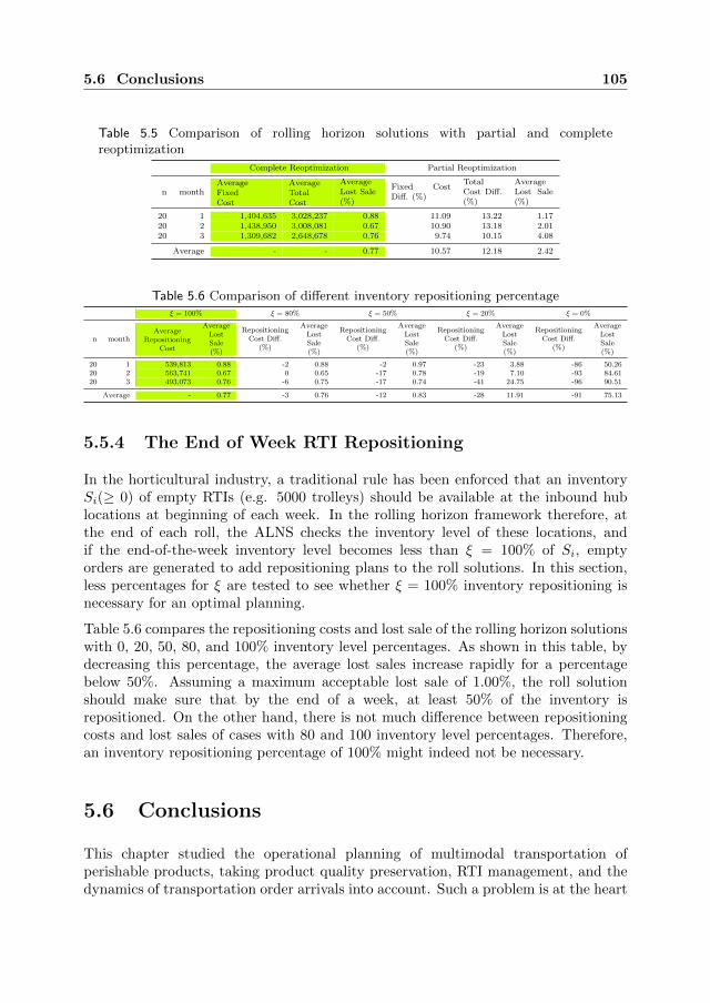
5.6 Conclusions 105
Table 5.5 Comparison of rolling horizon solutions with partial and completereoptimization
Complete Reoptimization Partial Reoptimization
n monthAverageFixedCost
AverageTotalCost
AverageLost Sale(%)
Fixed CostDiff. (%)
TotalCost Diff.(%)
AverageLost Sale(%)
20 1 1,404,635 3,028,237 0.88 11.09 13.22 1.1720 2 1,438,950 3,008,081 0.67 10.90 13.18 2.0120 3 1,309,682 2,648,678 0.76 9.74 10.15 4.08
Average - - 0.77 10.57 12.18 2.42
Table 5.6 Comparison of different inventory repositioning percentageξ = 100% ξ = 80% ξ = 50% ξ = 20% ξ = 0%
n monthAverage
RepositioningCost
AverageLostSale(%)
RepositioningCost Diff.
(%)
AverageLostSale(%)
RepositioningCost Diff.
(%)
AverageLostSale(%)
RepositioningCost Diff.
(%)
AverageLostSale(%)
RepositioningCost Diff.
(%)
AverageLostSale(%)
20 1 539,813 0.88 -2 0.88 -2 0.97 -23 3.88 -86 50.2620 2 563,741 0.67 0 0.65 -17 0.78 -19 7.10 -93 84.6120 3 493,073 0.76 -6 0.75 -17 0.74 -41 24.75 -96 90.51
Average - 0.77 -3 0.76 -12 0.83 -28 11.91 -91 75.13
5.5.4 The End of Week RTI Repositioning
In the horticultural industry, a traditional rule has been enforced that an inventorySi(≥ 0) of empty RTIs (e.g. 5000 trolleys) should be available at the inbound hublocations at beginning of each week. In the rolling horizon framework therefore, atthe end of each roll, the ALNS checks the inventory level of these locations, andif the end-of-the-week inventory level becomes less than ξ = 100% of Si, emptyorders are generated to add repositioning plans to the roll solutions. In this section,less percentages for ξ are tested to see whether ξ = 100% inventory repositioning isnecessary for an optimal planning.
Table 5.6 compares the repositioning costs and lost sale of the rolling horizon solutionswith 0, 20, 50, 80, and 100% inventory level percentages. As shown in this table, bydecreasing this percentage, the average lost sales increase rapidly for a percentagebelow 50%. Assuming a maximum acceptable lost sale of 1.00%, the roll solutionshould make sure that by the end of a week, at least 50% of the inventory isrepositioned. On the other hand, there is not much difference between repositioningcosts and lost sales of cases with 80 and 100 inventory level percentages. Therefore,an inventory repositioning percentage of 100% might indeed not be necessary.
5.6 Conclusions
This chapter studied the operational planning of multimodal transportation ofperishable products, taking product quality preservation, RTI management, and thedynamics of transportation order arrivals into account. Such a problem is at the heart

106 Chapter 5. A Rolling Horizon Framework for Operational Planning
of any DSS used in practice.
A rolling horizon framework was presented, where the MIP of Chapter 3 with dynamicparameters and inputs is periodically reoptimized by means of a modified version ofthe ALNS algorithm of Chapter 4.
The presented framework was tested on three sets of 7, 11, 20 location instances overtotal time period of three months. The overall results show that product perishabilityenforces truck-only forward flows in general, but when economy of scale allows andit is time-wise feasible, barge is also favored. For backward flows of empty RTIs,this transportation system makes a good use of the multimodal infrastructure, butif economy of scale does not allow, and RTIs should be urgently repositioned, trucksare substantially used.
The length of a roll, denoted as τ , also has a significant influence on the quality ofsolutions, showing a trade-off between the costs and lost sale. The shorter (closerto real-time) τ is, the less sale is lost. However, because less orders were collectedand there is no anticipation of what future orders would be, the operational costsincrease due to less consolidation possibilities and less flexibility. For shorter τ forexample, an order might be planned to start its transport right in the next roll withtransport modes dedicated only to this order, while with longer τ , the same ordermight be consolidated with other ones, resulting in less usage of modes. The averageacceptable total lost sale is a key to choose the best τ . A replanning strategy, asshown in the results, significantly improves this, and it is necessary not to excludefuture roll plans, if they have not been executed yet.
Finally, compared to practice, where 100% of the empty RTI inventory are reposi-tioned by the end of week, the presented analysis show that a 100% repositioning isnot necessary. The trade-off between costs and acceptable total lost sales is reachedby having a repositioning rule between 50% and 80%. It is important to note that thisrepositioning rule might have a different value or setup for other perishable industries.
Possible future work can be to include the uncertain nature of some system elements.The horticultural sector of the Netherlands deals with highly perishable and valuableproducts, and even a small percentage of lost sale per day is not desirable. Therefore,it is wise to include an anticipation of future demand as stochastic order volumes intothe rolling horizon. Chapter 6 in particular, incorporates anticipation of demand intothe operational planning.

Chapter 6
A Scenario-based StochasticRolling Horizon Frameworkfor Operational Planning withDemand Uncertainty
Following Chapter 5, the current chapter addresses the operational planning problemof multimodal long-haul transportation of perishable products. In Chapter 5, theoperational planning problem was explored and a rolling horizon framework wasdesigned for it, where based on known customer orders, available transportationmodes, and the evolution of operations, a reoptimization problem is periodically solvedto provide relevant responses to new orders and possible updates to the transportationand repositioning plans. This rolling horizon framework only takes the available datainto account, and does not have any perception of the future. In practice although,there are many sources of uncertainty, and including an anticipation of them into theoperational planning might bring opportunities for more efficient operation, which arenot detected by only using the known data. This chapter includes uncertainty and inparticular, uncertainty of customer demand in the operational planning. Section 6.1gives a description of the problem and its uncertain nature, and Section 6.2 reviewsthe related literature. Section 6.3 then takes a look at different modeling of stochasticcustomer demand, presents the Scenario-based Two-Stage Program (STSP) used todeal with this stochasticity, and explains the modifications and additions to the rollinghorizon framework. Section 6.4 gives a detailed computational analysis, and finallyin Section 6.5, some concluding remarks are provided.

108 Chapter 6. A Scenario-based Rolling Horizon with Uncertain Demand
6.1 Problem Description
Chapter 5 described and modeled the operational planning problem of the long-haultransportation of perishable products with repositioning of Returnable TransportItems (RTIs). In that problem, after specific time intervals of e.g. every 12 hours,based on revealed customer orders by then, available services and modes, and stateof the planned operations, a truncated optimization problem was solved to provideefficient new and updated plans for a planning horizon of e.g. the coming 72 hours,in order to respond to the arrived customer orders and system evolution.
In Chapter 5, only accessible and known data is contemplated and the future beyondthat is unknown. It is argued that an indication of future can help reducing variousplanning stresses and costs, as well as reaching higher levels of customer service.By considering future demand, there would be a chance to recognize consolidationopportunities in future time intervals, which would result in cheaper and moreefficient transportation. Such opportunities become a motivation for modeling andincorporating anticipation in the planning.
In reality, nothing in future is deterministic, and depending on sensitivity of plansto the future uncertainty, the following sources of uncertainty can be considered inlong-haul transportation planning:
� Customer demand, characterized by origin and destination locations, volumeof items to be transported, and desired scheduling of delivery. In sometransportation problems, only volume to be transported is uncertain, butin others, the scheduling, the volume, and even the location of customer isuncertain. For instance, in courier planning, customer locations are knownwhen orders to deliver their packages are revealed.
� Service time and travel time. In congested logistics locations, such as cross-docks and intermdal hubs, delays in service time are not known until the actualtime for a service. Likewise, delays caused by traffic or accidents are not knownuntil arrival to the area of such disruptions.
� Resource availability, capacity, and price. Resources can be vehicles, labor,energy, etc., and their capacity, costs, and even their availability, especiallywhen they are contracted or rented, can become sources of uncertainty,
� Technical conditions. In transportation of perishable products where productsare handled and moved in conditioned environments and fleet, change intemperature, humidity, etc., can cause uncertainty in the product freshnessevaluations.
Depending on how much historic knowledge is available on each of these and howsensitive the system evolution is to their fluctuation, each source of uncertainty istreated differently. Regarding sensitivity of plans, for instance, in a same-day city

6.1 Problem Description 109
Figure 6.1 Demand for flowers for Amsterdam in year 2013 (based on number of RTIs)
(a) Demand volume change in 2013(b) Histogram of demandvolume
Figure 6.2 Demand of Amsterdam on day 1 of the week
(a) Demand volume change in 2013(b) Histogram of demandvolume
Figure 6.3 Demand of Amsterdam on day 6 of the week

110 Chapter 6. A Scenario-based Rolling Horizon with Uncertain Demand
distribution planning problem where plans are sensitive to shortest delays (caused bye.g. traffic), it is necessary to contemplate stochastic nature of travel times into theplanning. In contrast, in long-haul transportation of products, where travel timesare in the order of hours and days, using expected values for travel times might besufficient to guarantee an efficient operational plan.
In deterministic planning problems, by making some assumptions, all sources ofuncertainty are treated as deterministic. In operational planning problems, relaxingall of these assumptions results in a large, complex, and intractable problem whichis not easy to solve. Therefore, the majority of them are kept deterministic and onlythe most influential source(s) are contemplated as stochastic.
Customer demand is the first and foremost source of uncertainty. In perishableindustries, customer demand is non-stationary, and there are daily, weekly, seasonal,and promotional trends influencing the volume of products that a customer orders. Togive an example, Figure 6.1 shows how drastic the daily volume of flowers ordered bycustomers in Amsterdam, changes throughout a year. The most significant trend inthis figure is the repetition of a weekly trend. Figures 6.2a and 6.2b show the volumedistribution for the first day of week, and Figures 6.3a and 6.3b show the distributionfor the weekends throughout a year. These figure show that the sale of flowers duringweekends is much higher than other days meaning that the volume of orders relatedto those days are higher than others. In addition to weekly trends, seasonal trend canbe seen in these figures, with more products transported in spring and summer whenthe flowers are harvested mostly. These trends encourage daily control and tailoredplans to guarantee the operation efficiency.
Uncertainty, especially when plans are fixed a priori, might cause capacity shortagein the arranged multimodal fleet, which would influence transportation of productsdirectly, or indirectly by late repositioning of empty RTIs. If the realization of demandfor future time intervals is less than their expected values, there would be no problemand the planned fleet capacity would be sufficient to transport the products andreposition the empty RTIs. However, when the realized demand of future is morethan the planned capacity, companies resort to outsourcing the operations, urgentrenting of extra transportation options and employing additional resources. Theselast-minute measures, called ad-hoc capacity increase [Hoff et al., 2010], are usuallymuch more expensive and inefficient. These decisions and their associated costs shouldbe included in operational planning, so that the new plans prevent such burdens andthe risk of overpaying for the extra reservation and RTI movements. This chaptertakes uncertainty of customer demand and its consequential operational issues intoaccount, and leave other sources of uncertainty as deterministic.
In operational planning of this chapter, assuming to have 1) access to the plans andthe state of system from previous time interval, 2) a good anticipation of customerdemand, and 3) good expected values for the other sources of uncertainty such thatthey can be treated as deterministic, the main decisions of this operational planningproblem are as the followings:

6.1 Problem Description 111
� flow of new customer demand revealed in previous time intervals,
� flow of anticipated customer demand in the coming time intervals,
� new and updated repositioning of Returnable Transport Items (RTIs) for bothrevealed and anticipated demand,
� new and updated selection of transport modes and schedules, which transportthe revealed customer demand, while preparing for future demand fluctuations,
� new and updated number of vehicles (real and ad-hoc) needed for each of thesetransport modes.
The main decisions are again defined on the RTI flow, repositioning, handling, andholding throughout the network and over the given planning horizon. Compared tothe decisions in Chapter 5 however, the fleet arrangement not only serves the knownRTI flows, but is also prepared for anticipated ones.
Demand is represented by orders. In this chapter, there are two sets of orders: realand future orders.
Real orders arrive to the system at different time periods of a time interval. A realorder is characterized by its pair of origin and destination locations, its volume, itspickup and delivery schedules, and its freshness requirements. Since RTIs are theloading units used to transport the products, the order volume shows the number ofRTIs (e.g. 2 trolleys) needed to transport products from the origin to the destination.The products can be picked up and loaded onto the RTIs at an earliest given time,and should be delivered to the destination and unloaded at a latest given time. Theseschedules are not definite though, and as long as the order is transported within thelength of this schedule, its flow is feasible. For instance, an order might be held fora few hours at its origin destination before it is loaded and transported. Similar toChapter 3, product freshness is approximated by a Time Temperature Sum (TTS)measure, and a maximum limit is enforced on TTS of orders.
Future orders are generated based on historic information about the demand forproducts ordered by each customer in future time intervals. Their locations, pickupand delivery time windows, their volume, and desired TTS, can all be subjects ofuncertainty.
In order to transport RTIs over the given planning horizon, fleets of differenttransportation modes over the coming planning horizon are assumed availablethroughout the network. Each transport mode has its given schedules, and its vehiclesoperate based on them. Each mode has a specific temperature, which for exampleshows the temperature inside a truck trailer, a train car, or a barge storage room.Vehicles of a transport mode are capacitated (here, based on RTIs), and there arelimited number of vehicles available for each transport modes. In comparison totactical planning problem however, the characteristics of available fleet is dynamic,and from one time interval to the next, might be different.

112 Chapter 6. A Scenario-based Rolling Horizon with Uncertain Demand
The objective function of this operational planning problem can also be dynamic, ifcosts of available transportation modes and services change over different planninghorizons. For instance, it might be cheaper to rent a truck tomorrow than to rent ittoday. Moreover, depending on how much operations are based on a priori fixed plans,an objective function of operational planning problems can have different forms. Inthis chapter, the objective function is to minimize total operational costs, includingflow costs of the loaded RTIs, flow costs of the assigned and repositioned empty RTIs,locational costs, costs of using the modes to carry out these tasks, and finally thecosts of ad-hoc capacity increase, over all rolled planning horizons.
6.2 Related Literature
There is no unique way in modeling and solving operational planning problems withstochastic elements. Depending on what insights are needed from incorporating theseelements, how much information is available on their behavior, what the length ofa planning horizon is, how far the uncertainty should be anticipated, etc., there aremany approaches in dealing with stochastic elements in the literature.
Operational planning of long-haul transportation of perishable products with repo-sitioning of RTIs, can be placed as special class of dynamic and stochastic trans-portation planning literature. The most important and frequently used approachesfor modeling and solving dynamic and stochastic problems are [Powell, 2009]:
� Simulation-optimization, where a good set of parameters is obtained by meansof simulation and optimization search tools.
� Rolling horizon procedures, where using deterministic or stochastic forecasts, aplanning problem is periodically solved.
� Dynamic programming, where decisions are made with an estimate of the valueof states to which an action might result in.
A portion of the literature is dedicated to the application of Approximate DynamicProgramming (ADP) in resource allocation and management. ADP was developedto tackle the curse of dimensionality in solving stochastic and dynamic problems.In this regard, several search and value function approximation policies have beenintroduced in the literature. Powell et al. [2012] provide a tutorial of the modeling andalgorithmic framework of ADP in transportation and logistics planning. Topalogluand Powell [2006] extend previous works on ADP models for fleet management toinclude heterogeneous resources and substitution among them. Their method uses ahybrid of linear and piecewise-linear approximations of the value function. Topalogluand Powell [2007] develop sensitivity analysis methods for a stochastic dynamic fleetmanagement model to compute the change in the objective value in response to

6.2 Related Literature 113
changes in fleet size and load availability. In other words, they demonstrate how tocompute the objective function of the model due to changes in vehicle or (and) loadpresented in the system. Topaloglu and Powell [2005] extend the dynamic resourceallocation problem to a distributed decision-making case. They use an ADP wheredifferent agents make the decisions regarding the resources. They use nonlinearfunctional approximation to model the coordination of actions of different agents.Lam et al. [2007] apply Approximate Dynamic Programming (ADP) to an emptycontainer allocation problem arising in a sea-cargo industry. They first model a simpletwo-port two-voyage system and extend it to multi-port multi-voyage network. Lamet al. [2007] propose a simulation based Approximate Policy Iteration (API) algorithmwhich shows significant performance improvement compared to the heuristics used inpractice. Bouzaiene-Ayari et al. [2014] propose an ADP framework for a rail fleetsizing and routing problem, with a streamlined single commodity model, a moredetailed multicommodity model, and a multiattribute model. They show that ADP ismuch faster than a state-of-the-art Integer Programming (IP) solver, and can providesolutions for large and complicated problems with several stochastic elements.
Rolling horizon approaches were introduced and reviewed in Chapter 5. Theapplication of rolling horizon methods with stochastic elements is limited. An exampleis Di Francesco et al. [2013]. They study the effect of partial or complete portdisruption in empty container repositioning in a liner shipping system. They modelit as a time-space representation and consider a set of different disruption scenarios.They also include some non-anticipativity conditions to equalize the here-and-nowdecision variables over all scenarios. Di Francesco et al. [2013] test all combinationsof a problem including 5 locations (2 hubs), a 50 period rolling horizon scheme, 2(normal and disrupted) scenarios, and 2000 customer orders. They show that in caseof a normal scenario, the optimal deterministic solutions are the best, but in case of adisruption, the multi-scenario model produces the most effective results. Di Francescoet al. [2013] show their model is able to handle 12 disruption scenarios with up to 20locations in less than one hour.
Rolling horizon and simulation-optimization approaches have the opportunity toaccommodate any existing modeling and algorithm methods in the literature ofstochastic tactical and strategic planning. The literature on tactical long-haultransportation planning where at least one aspect of the problem is uncertain hasbeen vastly studied.
Assuming that an anticipation to that future uncertainty is available, there are twoapplications for it in the literature: 1) to design a robust system, or 2) to plan aflexible one.
A robust system is a system capable of withstanding any range of uncertainty. It isdesigned and fixed a priori to the realization of uncertain factors. Atamturk and Zhang[2007] propose a two-stage robust optimization for multicommodity network flow anddesign problems with stochastic demand. They introduce a “budget for demanduncertainty” parameter, which allows control, and provides an upper bound on the
114 Chapter 6. A Scenario-based Rolling Horizon with Uncertain Demand
probability of infeasibility. They compare this approach with single-stage robust aswell as a Scenario-based Two-stage Stochastic Program (STSP), and showed that theirrobust two-stage model offers an interesting trade-off between the other two classicapproaches. Moreover, unlike the two-stage optimization, it does not need to generatea large number of scenarios and therefore, it is much faster. An and Lo [2014] alsostudy a ferry Service Network Design (SND) problem with stochastic demand andconsidering user equilibrium flow. They formulate it as a STSP where they introducea service reliability measure into the model to be able to tackle the complexity ofthe model via solving a sequence of mixed-integer linear programs. Shu and Song[2013] propose a general two-stage robust optimization for a container managementproblem, and discuss its computational complexity, and compare it with deterministicand stochastic counterparts. Demir et al. [2015] study an intermodal transportationplanning problem with stochastic demand and travel times, and with emission-relatedcosts. They propose a continuous-time mixed-integer linear programming formulationfor it, and apply a Sample Average Approximation (SAA) algorithm which evaluatesan extensive set of scenarios in order to develop more robust transportation plans.Cacchiani et al. [2012] take railway network disruption into account and present a two-stage optimization model to determine a robust rolling stock circulation. They modelit as a Mixed-Integer Linear Program (MILP). Then they use Benders decompositionand its generated cuts to find heuristic solutions for this problem. They show thattheir solution approach is fast and generates quality solutions, especially with largenumber of disruption scenarios. Garg and Smith [2008] design an efficient algorithmto solve a capacitated multicommodity flow network design with arc failure whereat each time, multiple arcs are simultaneously fail, and the algorithm needs toprovide new adjustments in short time. In this regard, they use augmentation inthe master problem, with Benders decomposition with cover constraints providingthe best result for real-size instances, and Benders decomposition augmented byexplicit multicommodity flow conditions performing best in cases with small numberof failures.
A flexible system in comparison, is a system that is able to provide optimal actionswhen an uncertain factor is realized. These actions are not fixed a priori, anddepending on scenarios included in the planning, they can change. Lium et al.[2009] study SND problems with stochastic demand and model it as a STSP. Theythen provide an analysis in structural differences and the role of consolidation inuncertainty cases with high and little commodity demand correlations. As a futureresearch, they suggest use of their study in designing heuristic algorithms for similarproblems. Crainic et al. [2011] propose a progressive hedging-based metaheuristicalgorithm to solve a two-stage stochastic service network design problem and showthat their algorithm outperforms any state-of-the-art solver. They use scenariodecomposition to separate the stochastic program and solve these scenario-subproblemin parallel and via different strategies that guides them towards the optimal design.Crainic et al. [2014] study and analyze scenario grouping by introducing strategiesinto a progressive hedging-based metaheuristic, where these strategies are defined by

6.3 Modeling Approach and Solution Algorithm 115
the type of scenario decomposition (partition or cover), type of grouping, and thescenario similarity measures (demand-based or service-based). They propose threegrouping strategies: group similar scenarios, group similar scenarios but introduce adissimilar group, and group dissimilar scenarios. They show that their multi-scenariosubproblems produce find better solutions in shorter time compared to a state-of-the-art solver and compared to randomly scenario grouping strategy, the best beingthe covering strategy with respect to demands. Di Francesco et al. [2013] studyrepositioning of maritime containers under port disruption uncertainty, and model itas STSP. Van Hui et al. [2014] also model a airfreight shipment forwarding problemin the presence of delays, which they solve by Tabu Search.
The current chapter adds to the literature of operational planning of long-haultransportation by applying rolling horizon methods, where a scenario-based stochasticprogram is used to deal with uncertainty of demand. The next section describes thisapproach in detail.
6.3 Modeling Approach and Solution Algorithm
The previous section pointed at three methods of simulation-optimization, rollinghorizon, and dynamic programming, to deal with dynamic and stochastic problems.In choosing the best approach, besides modeling strategies for the uncertainty,dimensions of the model is a critical factor. If the range of values or states theuncertain element has, is relatively wide, the dimensions of the stochastic modelexplode and solving it would be impossible. As a result, approximation methodsare used to reduce this dimension via logical simplifications. Approximate dynamicprogramming (ADP) methods have specially been developed for such cases. ADPhas shown to be a powerful modeling and algorithm design tool, however, is noteasy to implement [Powell, 2009]. If there is good information on the behavior ofthe uncertain elements, and the stochastic problem is solved using relatively simplermethods, there is no need for ADP. Finding a value function approximation thatrepresents the structure of the problem is not straightforward. Formulating its searchstructure and stepsize is also tricky.
In previous chapters of this thesis, a few models and solution algorithms wereproposed that can easily be employed here. Chapter 5 proposed a rolling horizonframework, where a small optimization problem is periodically solved. This problem isdeterministic and includes decisions related to only known data and system evolution.In this chapter, future demand uncertainty is added to the proposed rolling horizonframework.
There are several strategies which can be used when demands are uncertain [Powellet al., 1995]:
� Deterministic modeling, where demand is simply estimated and then treated

116 Chapter 6. A Scenario-based Rolling Horizon with Uncertain Demand
deterministically within the model. This model would be identical to theprevious ones, except that some of the demands would represent real orders,and others would be expectations of forecasts.
� Chance constrained programming, where capacity constraints would be replacedwith a probabilistic inequality and solved as a nonlinear programming problem.
� Stochastic programming. It is the most rigorous modeling and solutionframework, but also the most complex one. In this approach, the problemis optimized over the known and future demand, taking the expected costs ofresponding to various demand outcomes (scenarios) into account.
In this chapter, stochastic programming is chosen to deal with demand uncertainty.It can easily be extended from the previous models, and be solved by the proposedalgorithms. In the remainder of this section, first, the modified rolling horizonframework is described. Then, anticipation of future demand is defined, where apopulation of scenarios are generated for. Furthermore, a Scenario-based Two-stageStochastic Program (STSP) is formulated to optimize a truncated problem used in therolling horizon framework. Finally, the Adaptive Large Neighborhood Search (ALNS)algorithm is used to solve the STSP, and a simulation step to evaluate its solutions,are explained.
6.3.1 Rolling Horizon Framework
The rolling horizon framework of this chapter is an extension to the framework ofChapter 5, but at the end of a roll φ and after collecting new data, an anticipation ofdemand (via generating a population of scenarios) for future time intervals is made.Then a STSP problem with time periods t = φ, φ + 1, . . . , φ + T is solved to derivenew plans and adjustments for the following horizon of T . Then, the new plans areexecuted until the end of roll φ+ 1. The collected data includes the set of new ordersarrived during roll φ, as well as the state of the system and resource availability bythe end of roll φ.
In order to be able to analyze efficiency of the arranged fleet in a stochastic solution,this framework includes two tracks, one for solving the STSP, and one for solvinga deterministic planning counterpart, where a deterministic Mixed-Integer Program(MIP) with expected average daily demand for future time intervals is solved.The deterministic solution is later put into simulation to find how it responds touncertainty depicted by the scenarios. Figure 6.4 highlights the additions to theextended framework.
The objective function of both truncated problems is then to minimize totaloperational costs, including flow costs of the loaded RTIs, flow costs of the assignedand repositioned empty RTIs, locational costs, costs of using the modes, and finally,the costs of ad-hoc capacity increase, over the planning horizon T . The length of T is

6.3 Modeling Approach and Solution Algorithm 117
Figure 6.4 The planning algorithm plus simulation
now set to be equal to the latest delivery due date among all collected orders of rollφ and the anticipated customer orders.
6.3.2 Anticipation of Future Demand and Its Related Costs
At the end of each roll (here, a day), orders of today p = 1, . . . ,P have been realizedand all their volume wp are known, but orders of future days and their volumes areunknown. Each future order p′ ∈ {1, . . . ,P ′}, is characterized by the random numberwp′,day,week,season of RTIs ordered, with distribution function Ψ(wp′,day,week,season),and average number µp′,day,week,season. This distribution is non-stationary and thereare seasonal, weekly, daily, (and even hourly and promotional) trends influencing itsvalue. However, from one day to another, and from one customer to another, theyare independent. Adding to the fact that the rolling horizon algorithm of this chaptermakes daily anticipations, for simplicity, in the rest of this chapter, the randomdemand volume for each p′ is only denoted as wp′ with daily average of µp′ , andthe other factors are assumed to be inclusive in its distribution Ψ(wp′). In otherwords, for instance, if there is a weekly trend, for each week, a particular distributionΨ(wp′) is defined for each p′ of that week.
A naive way to plan for future days is to include orders p′ with their daily averages µp′
into the relevant MIP, and treat the model as a deterministic one. If the realization ofdemand for future days is less that the daily averages µp′ , there would be no problem

118 Chapter 6. A Scenario-based Rolling Horizon with Uncertain Demand
(a) Day 1 (b) Day 5
Figure 6.5 Daily demand frequency distribution of day 1 and day 5 of a week
and the planned fleet capacity for the next days would be able to transport theproducts and reposition the empty RTIs. However, when the anticipated demand forfuture days is more than the total planned capacity, companies resort to outsourcingthe operations related to low-volume orders. This option and its associated costsshould then be included into the planning. In this regard, an ad-hoc fleet capacityincrease, denoted as θp′ and its associated cost per unit Cθ for p′ = 1, . . . ,P ′ areadded to the model to reflect the amount of order volume that is outsourced.
The distribution function Ψ(wp′) can be discrete or continuous [Lium et al., 2009], butif the behavior of customer demand is not known and only historical data is available,a comprehensive statistical analysis is required to find this function, and such analysisis out of scope of this thesis. For this thesis, only historical data of year 2013 wasavailable [Tosi, 2014, Verhoeven, 2014, Vlassak, 2014, Rosenboom, 2014], which wasanalyzed and translated into frequency distribution of daily demand volume for eachcustomer p′ [Rubin, 2010].
These frequency distributions are used to represent all possibilities of wp′ and theirprobability Ψ(wp′). It is important to note that the relevant daily, weekly, seasonaltrends are considered in generating these distributions. Figures 6.5a and 6.5b giveexamples for the daily demand frequency distribution for city of Amsterdam.
6.3.3 Scenario Generation
Even with having the frequency distribution of demand at hand, including allpossibilities of wp′ for all orders p′, make a stochastic program too large and complexto solve to optimality. In operational planning problems, where new plans and neededadjustments should be made in a really short time of a few minutes to a few hours, thesize of the stochastic program becomes troublesome. For instance, if the frequencydistribution of wp′ has a range of 50 RTIs to 150 RTIs for each p′, the size of a

6.3 Modeling Approach and Solution Algorithm 119
deterministic counterpart MIP expands by (P ′)100.
In order to have a manageable stochastic program, for each order set p′, a set of γ =1, . . . ,Γ scenarios with uniform probability of ργ are generated, and the deterministicMIP of Chapter 3 is extended to include these scenario realizations and becomes aScenario-based Stochastic Program (SSP). In the following sections, this stochasticprogram and its two stages are formulated.
6.3.4 Scenario-based Two-Stage Program with Stochastic De-mand
In this section, the mathematical formulation for the STSP with stochastic demandof roll φ is explained. Note that for simplification reasons, the dimension of φrepresenting a roll in the rolling horizon framework is removed from the STSPformulation, but in fact, this model can have different parameter setting and numberof variables in each roll φ, depending on order sets P and P ′, and the availabletransportation modes.
Demand is defined as orders. A real order p is characterized by the number wp of RTIsneeded to load and transport products from an origin location O(p) to a destinationlocation D(p). The products can be picked up and loaded onto the RTIs at an earliesttime of PT (p) and should be delivered to the destination and unloaded at the latesttime of DT (p). Product freshness preservation is evaluated by Time TemperatureSum (TTS) measure, and for each order, it is assumed that the summation of theseTTS’s should be less than Lp (say 200 hours× degree).
Fleets of different transportation modes over the coming planning horizon, with givenschedules, temperature, capacity, and number of available vehicles are available. Incomparison to the tactical planning problem though, the characteristics of availablefleet is roll-dependent, and from one roll to the next, might be different.
At the end of each day, a set of γ = 1, . . . ,Γ scenarios with uniform probability of ργare generated. Each scenario is a set of future orders. A future order p′ ∈ {1, . . . ,P ′}is distinguished by its random volume wp′ with daily average of µp′ and a distributionfunction Ψ(wp′). An ad-hoc fleet capacity increase, denoted as θγp′ for p′ = 1, . . . ,P ′
is added to the model to reflect the amount of order volume that is outsourced. Theassociated cost per unit is Cθ, which is later added to the objective function.
The goal of this Scenario-based Stochastic Program (SSP) is to find a flexiblemultimodal fleet to answer all realization of random demand volumes of future ordersp′, as well as the known volume of orders p. Therefore, the SSP is reformulated intotwo stages, where in the first stage, the transportation mode fleet is arranged and theRTI flows and repositioning of real orders are planned. In the second stage then, thearranged fleet with the remaining resources and capacities are used for transportingthe products and repositioning the RTIs for future scenario orders.

120 Chapter 6. A Scenario-based Rolling Horizon with Uncertain Demand
As described in Chapter 5, an objective function of operational planning problemis also roll-based and can have different forms. In this chapter, the objectivefunction of of the operational planning and its embedded STSP is to minimize totaloperational costs, including flow costs of the loaded RTIs, flow costs of the assignedand repositioned empty RTIs, locational costs, and finally, costs of using the modes,over all rolled planning horizons. Note that there is no cancellation or change of pathfor the moving modes.
Let A1 = {a(i,j),t,(m1,m2) ∈ A(V × V) | i 6= j,m1 = m2} be the set of all feasible andgiven travel arcs, and let A2 = {a(i,j),t,(m1,m2) ∈ A(V×V) | i = j,m1 = H ‖ m2 = H}be the set of all feasible location arcs, representing loading, unloading, holding andwaiting arcs. Similarly, let Am = {a(i,j),t,(m1,m2) ∈ A(V × V) | m1 = H ‖ m2 = H}be the set of all feasible loading, unloading, traveling, and waiting arcs in the networkrelated to mode m.
For each order p or p′, there are three flow decisions: laden, assign, and repos flowdecisions, and there are two sets of variables defined for each of them: 1) x to showhow many RTIs enter an arc a(i,j),t,(m1,m2), and 2) x to show how many RTIs exit thearc. Likewise, there are two sets of variables y and y to show the number of vehiclesrespectively entering and exiting an arc. The auxiliary binary variables b and b arealso added to help calculating TTS of real and future orders. Three variables U arealso added to the model to keep track of the inbound and outbound flows at eachlocation, and to connect the flows of loaded and empty RTIs throughout the network.
The roll-dependent STSP model with product quality preservation and empty RTImanagement is then formulated as follows:
First Stage
Compared to a classic STSP, in this chapter, the first stage not only includes fleetarrangement decisions y and y, but also includes decisions x and x on the RTI flowand repositioning of the real orders. No matter what scenario is realized for futureorders, the real orders are planned in this stage. Therefore, their related decisions areplaced in the first stage.
As a result, with some parameter modifications, the first stage problem is in the formof minimizing the first stage costs of the STSP, which is the total costs of using thefleet in (3–1e), as well as costs related to real order variables in (3–1a)-(3–1d). Thisobjective function is then subject to Constraints (3–2)-(3–7), (3–8), (3–9)-(3–11),(3–13) and (3–14), (3–15), (3–17), and (3–18)-(3–20).
Note that repositioning decisions only become positive, if RTIs are needed to berepositioning during the current planning horizon t = φ, φ+1, . . . , φ+T . In Chapter 5,a end-of-the-week RTIs repositioning rule was applied. Let tstore be such a (repetitive)repositioning deadline. If tstore > φ+ T , all repositioning decisions become zero.

6.3 Modeling Approach and Solution Algorithm 121
Second Stage
The objective function of the second stage is in the form of minimizing the ad-hoccosts related to future orders over scenarios γ = 1, . . . ,Γ. Terms (6–1a) representflow costs of the loaded RTIs, the terms of (6–1b) are the flow costs of the assignedand repositioned empty RTIs respectively, the term (6–1c) shows locational costs ofloaded RTIs, the terms (6–1d) represent locational costs of assigned, and repositionedRTIs, for each scenario orders. Finally, (6–1e) is the costs of using ad-hoc capacityincrease in a scenario.
Similar to the first stage, the scenario-based repositioning decisions become positive,if it is required to return RTIs to their initial storage during the current planninghorizon t = φ, φ+ 1, . . . , φ+ T .
Constraints (6–2)-(6–5) are variable pair matching of future scenario orders. Theirlogic is similar to the Constraints (3–2)-(3–7).
min
Γ∑γ=1
∑a(i,j),t,(m1,m2)∈A1
r(m)(i,j),t
P′∑p′=1
Cmladen
(xγ,ladenp′,(i,j),t,(m1,m2)
) (6–1a)
+∑
a(i,j),t,(m1,m2)∈A1
r(m)(i,j),t
P′∑p′=1
Cmempty
(xγ,assignp′,(i,j),t,(m1,m2)
+ xγ,reposp′,(i,j),t,(m1,m2)
) (6–1b)
+∑
a(i,j),t,(m1,m2)∈A2
r(m1,m2)i,t
P′∑p′=1
C(m1,m2)i
(xγ,ladenp′,(i,i),t,(m1,m2)
) (6–1c)
+∑
a(i,j),t,(m1,m2)∈A2
r(m1,m2)i,t
P′∑p′=1
C(m1,m2)i
(xγ,assignp′,(i,i),t,(m1,m2)
+ xγ,reposp′,(i,i),t,(m1,m2)
)
(6–1d)
+Cθ
Γ∑γ=1
ργ
P′∑p′=1
θγp′
(6–1e)
xγ,catp′,(i,j),t,(m1,m2)
= xγ,catp′,(i,j),(t+rm
(i,j),t),(m1,m2)
∀cat ∈ {laden, empty, repos},a(i,j),t,(m1,m2) ∈ A1
p′ = 1, . . . ,P ′γ = 1, . . . ,Γ
(6–2)
xγ,catp′,(i,i),t,(m1,m2)
= xγ,cat
p′,(i,j),(t+r(m1,m2)i,t ),(m1,m2)
∀cat ∈ {laden, empty, repos},a(i,j),t,(m1,m2) ∈ A2
p′ = 1, . . . ,P ′γ = 1, . . . ,Γ
(6–3)

122 Chapter 6. A Scenario-based Rolling Horizon with Uncertain Demand
bγp′,(i,j),t,(m1,m2)
= p′γp,(i,j),(t+rm
(i,j),t),(m1,m2)
∀a(i,j),t,(m1,m2) ∈ A1
p′ = 1, . . . ,P ′γ = 1, . . . ,Γ
(6–4)
bγp′,(i,i),t,(m1,m2)
= bγp′,(i,j),(t+r
(m1,m2)i,t ),(m1,m2)
∀aγ(i,j),t,(m1,m2)
∈ A2
p′ = 1, . . . ,P ′γ = 1, . . . ,Γ
(6–5)
Constraints (6–6) are flow conservation constraints for future scenario orders. Theseconstraints define U as the flow (loaded RTIs, assigned empty and repositioned emptyRTIs) for each order at each location and time period. These equalities imply thatthe inbound flows to each node should be equal to its outbound flows.
Uγ,catp′it =
∑j∈V−{i}
∑t′>t
M+1∑m=1
xγ,catp′,(i,j),t,(m1,m2)
−∑
j∈V−{i}
∑t′<t
M+1∑m=1
xγ,catp′,(j,i),t,(m1,m2)
∀cat ∈ {laden, empty, repos},i ∈ V,t = φ, φ+ 1, . . . , φ+ Tp′ = 1, . . . ,P ′γ = 1, . . . ,Γ
(6–6)
Constraint set (6–7) enforces the flow of loaded RTIs (for scenario orders) betweenorigin and destination locations, with wγp′ for each scenario γ.
Uγ,ladenp′it + θγ
p′
= wγ
p′ i = O(p), t = PT (p)
= −wγp i = D(p), t = DT (p)= 0 o.w.
∀i ∈ V,t = φ, φ+ 1, . . . , φ+ Tp′ = 1, . . . ,P ′γ = 1, . . . ,Γ
(6–7)
Uγ,assignp′it + θγ
p′
≤ Sremi Sremi > 0, t = φ= −wγ
p′ i = O(p), t = PT (p)
0 o.w.
∀i ∈ V,t = φ, φ+ 1, . . . , φ+ Tp′ = 1, . . . ,P ′γ = 1, . . . ,Γ
(6–8)
Uγ,reposp′it + θγ
p′
= wγ
p′ i = D(p), t = DT (p)
≥ −Sstorei Sstorei > 0, t = tstore
0 o.w.
∀i ∈ V,t = φ, φ+ 1, . . . , φ+ Tp′ = 1, . . . ,P ′γ = 1, . . . ,Γ
(6–9)
Assuming Sremi in the second stage to be the remaining inventory of empty RTIsafter assigning some of them to the real orders in the first stage, Constraints (6–8)and (6–9), in a similar fashion enforce the flow of empty RTIs (for known orders)between origin and destination locations. The origin locations of the assigned emptyRTIs are the RTI storage locations with Sremi > 0. Their destination locations are thelocations that they are needed to be loaded and transport the products (O(p),PT(p)).
If repositioning decisions are made in roll φ, or in other words, tstore ≤ φ + T , therepositioned empty RTIs need to get back to their storage locations in the current

6.3 Modeling Approach and Solution Algorithm 123
roll. Therefore, the locations with Sstorei > 0 are their destinations and their originlocations are the locations that the loaded RTIs are unloaded (D(p),DT(p)).
Constraints (6–10) and (6–11) are logical constraints which are used to calculate theTTS of scenario orders. Note that M here is the classic “big M” and not the numberof modes. Based on these constraints then, if there is no flow of products on a specificarc (x = 0), that arc will not be included in the constraint on TTS (b = 0).
xγ,ladenp′,(i,j),t,(m1,m2)
≥ bγp′,(i,j),t,(m1,m2)
∀a(i,j),t,(m1,m2) ∈ A(V × V),p′ = 1, . . . ,P ′γ = 1, . . . ,Γ
(6–10)
xγ,ladenp′,(i,j),t,(m1,m2)
≤ Mbγp′,(i,j),t,(m1,m2)
∀a(i,j),t,(m1,m2) ∈ A(V × V),p′ = 1, . . . ,P ′γ = 1, . . . ,Γ
(6–11)
Based on Constraints (6–10) and (6–11), Constraint (6–12) states that for each knownorder, the total time×temperature of moving and handling an order must not exceedan allowed TTS of that order.
∑a(i,j),t,(m1,m2)∈A1
lm(i,j),t × rm(i,j),t × b
γp′,(i,j),t,(m,m)
+∑
a(i,j),t,(m1,m2)∈A2
l(m1,m2)i,t × r(m1,m2)
i,t × bγp′,(i,i),t,(m1,m2)
≤ Lp∀p′ = 1, . . . ,P ′γ = 1, . . . ,Γ
(6–12)
Constraint (6–13) is the capacity constraint. In each scenario γ, the total number ofRTIs (loaded or empty) for both real and future orders that is moved between i andj at time t, should be less than or equal to the total capacity of y vehicles of modem transporting them, if that mode is chosen in that scenario.
P′∑p′=1
(xγ,ladenp′,(i,j),t,(m,m)
+ xγ,assignp′,(i,j),t,(m,m)
+ xγ,reposp′,(i,j),t,(m,m)
)
+P∑p=1
(xladenp,(i,j),t,(m,m) + xassign
p,(i,j),t,(m,m)+ xrepos
p,(i,j),t,(m,m)
)≤ capm × y(i,j),t,(m1,m2)
∀a(i,j),t,(m1,m2) ∈ Amγ = 1, . . . ,Γ
(6–13)
Finally, Constraints (6–14)-(6–15) define the nature of variables in the formulation.
xγcatp′,(i,j),t,(m1,m2)
, xγcatp′,(i,j),t,(m1,m2)
≥ 0
∀cat ∈ {laden, empty, repos},a(i,j),t,(m1,m2) ∈ A(V × V),p′ = 1, . . . ,P ′γ = 1, . . . ,Γ
(6–14)
bγp′,(i,j),t,(m1,m2)
, bγp′,(i,j),t,(m1,m2)
≥ 0∀a(i,j),t,(m1,m2) ∈ A1,p′ = 1, . . . ,P ′γ = 1, . . . ,Γ
(6–15)

124 Chapter 6. A Scenario-based Rolling Horizon with Uncertain Demand
Similar to its deterministic counterpart, this optimization problem is too complex tobe solved by exact methods. In the following section, we describe the ALNS algorithmused to solve the stochastic and deterministic truncated problems in both tracks ofthe rolling horizon framework.
6.3.5 ALNS and Planning Process
As mentioned earlier, there are two tracks in the current rolling horizon framework,one deterministic, and one stochastic. Therefore, two ALNS algorithms are employedto replan and update the stochastic and deterministic roll solutions zφ. Comparedthe the ALNS of Chapter 4, these algorithms have new and redesigned destroy andrepair operators.
An optimal solution to the STSP is a solution with optimal flow, repositioning, andmode usage over all scenarios plus the realized orders and system evolution. In orderto generalize and simplify the search, the set of real orders is put into an additionalscenario Γ + 1 with probability equal to 1.0, so that ALNS treats them equally asa scenario. Now, the main reason to redesign the operators is to give the ALNSalgorithm better direction to work on both inter-scenario neighborhoods (A series),and intra-scenario neighborhoods (B series).
The following destroy operators are used to remove the routes of orders:
� one random order (R1) operator,
� two random orders (R2r) operator,
� three random orders (R3r) operator,
� two similar orders (R2s) operator,
� three similar orders (R3s) operator,
� two inter-scenario random orders (R2r-A) operator,
� three inter-scenario random orders (R2r-A) operator,
� two inter-scenario similar orders (R2r-A) operator,
� two intra-scenario similar orders (R2r-B) operator,
� three inter-scenario similar orders (R2r-A) operator,
� three intra-scenario similar orders (R2r-B) operator,
� one ad-hoc positive order (Rd) operator.
And repair operators are as the followings:
� cheapest path (Ip) operator,
� scheduling (Is) operator,

6.3 Modeling Approach and Solution Algorithm 125
� consolidate two orders (Ic2) operator,
� consolidate three orders (single) (Ic3s) operator,
� consolidate three orders (paired) (Ic3p) operator,
� insert ad-hoc zero path (Ipd) operator.
The first five destroy and five repair operators are similar to the ones in Chapter 4,but the rest of them are new to this chapter. In inter-scenario destroy neighborhoods,only paths of orders belonging to a particular scenario γ (or only the path of knownorders) are destroyed, in order to let the algorithm to search neighborhoods improvinga specific scenario. In comparison, intra-scenario destroy neighborhoods try to findimproved fleet arrangement, satisfying the needs of more than one scenario (orcombined with scenario Γ + 1).
A new one ad-hoc positive order (Rd) destroy and a new insert ad-hoc zero path (Ipd)repair operator is also introduced to the stochastic ALNS, in order to improve theneighborhood of orders p′ with θp′ ≥ 0. The repair operator Ipd tries to reinsert suchorders into the solution so that its θp′ becomes zero.
6.3.6 The Simulation
The two ALNS algorithms result in two (stochastic and deterministic) roll solutions.The cost of a stochastic solution is the total cost of fleet arrangement and flow plansfor both known and scenario orders. However, the cost of a deterministic solutiononly takes the cost of fleet arrangement and flow plans of known orders into account.It is obvious that stochastic solutions have many more vehicles and therefore, highercosts, but these solutions are not comparable to the deterministic ones yet. In orderto compare the efficiency of the stochastic and the deterministic fleet arrangement,the deterministic solution is simulated on all γ = 1, . . . ,Γ scenarios in the population.While simulating with a scenario, if the deterministic solution faces capacity shortage,extra vehicles are added, which results in extra costs. Summation of these extrasimulation costs and the deterministic solution costs are then comparable to thestochastic costs.
After simulation, the plans of roll φ + 1 are executed for both stochastic anddeterministic roll solutions, and state of the routes, the related orders, and fleet isupdated. Execution of plans in practice can be translated as the instructions that aresent to relevant departments, to start loading/unloading operations, transportation,etc. The updated deterministic and stochastic roll solutions are later used for thenext round of planning at the end of roll φ+ 1.
In the next section, the performance of the modified ALNS and the rolling horizonframework is evaluated in detail.

126 Chapter 6. A Scenario-based Rolling Horizon with Uncertain Demand
6.4 Computational Results
In this section, the rolling horizon framework of Section 6.3 with its modified ALNSis tested on three instance sets with 20 locations, 3 mode types of truck, train, andbarge, and the minimum end-of-the-week repositioning rate of ξ = 100%. Since onlydaily demand distribution of customer locations is available, and there is no furtherinformation on their hourly arrival, scenarios for future day demand are generatedonly once per day (e.g. in the final roll of the day). As indicated in Section 6.3.2,weekly and seasonal trends are implicit. For instance, if there is a weekly trend,for each week, a new set of daily demand distribution is formulated for that week.Moreover, it is also argued that the conclusions of Chapter 5 on the sensitivity of therolling horizon framework still hold in this chapter, and the focus of this section ismore on the influence of uncertainty, and how it is handled inside the framework.
The instance sets are identified by month = 1, 2, 3, similar to Chapter 5. The lengthof a roll τ is equal to 24 hours, which means that there are 90 rolls per instance.Therefore, out-of sample stability of the results is guaranteed.
6.4.1 Parameter Tuning
The ALNS algorithms of this chapter have slightly different settings. For example, thestopping criteria, representing the number of iterations that the best found solution isnot improved, are set π = 500 and η = 125 for the deterministic ALNS, and π = 1000and η = 250, for the stochastic one. Moreover, a computational time limit of 30minutes is set for the stochastic ALNS.
6.4.2 Scenario Population Size
The first and most important factor in designing an efficient stochastic rolling horizonframework is the size of population Γ. In order to have in-sample stability in theresults, the size of population should be adequate. If this value is small, there is arisk that the scenario population does not represent the future adequately, and if itis large, the computational burden for obtaining a good solution increases and mightnot be suitable for the rolling horizon framework.
Table 6.1, and Figures 6.6a-6.6c show the performance of stochastic ALNS, comparedto the deterministic one, with three population sizes of 20, 50, and 100. The columnsof table 6.1 represent the costs of roll solutions for the deterministic ALNS, extracosts of putting the deterministic solutions to simulation, the total deterministic andstochastic system costs. The table also shows the differences by percentage, as well asthe percentage of rolls that stochastic solutions were worse than their deterministiccounterpart.
First of all, the overall results show that on average and over all months, the stochastic

6.4 Computational Results 127
Table 6.1 Influence of scenario population size on costs
n month ΓRoll
Deter.Costs
A.D.(%)
RollDeter.Sim.Costs
A.D.(%)
TotalDeter.Costs
A.D.(%)
TotalStoch.Costs.
A.D.(%)
Avg.Cost
Diff. (%)
Rollswith
WorseStoch.
Sol. (%)
20 1 20 1,119,738 1.00 499,881 1.14 1,618,508 1.07 1,498,836 1.31 -4.55 2520 2 20 1,141,618 0.38 459,861 2.86 1,601,479 1.98 1,500,356 1.86 -2.47 4120 3 20 1,140,147 1.36 465,398 1.35 1,605,544 1.36 1,479,537 0.91 -5.59 34
20 1 50 1,119,738 1.00 581,869 1.87 1,701,606 1.13 1,436,707 0.69 -12.61 2320 2 50 1,141,618 0.38 533,160 2.57 1,674,778 1.54 1,451,712 0.80 -8.75 2920 3 50 1,140,147 1.36 529,676 0.88 1,669,823 1.21 1,472,627 0.46 -9.09 23
20 1 100 1,119,738 1.00 596,139 0.80 1,715,877 1.10 1,429,859 0.68 -13.55 1920 2 100 1,141,618 0.38 555,251 0.59 1,696,869 0.41 1,444,558 1.77 -10.52 2520 3 100 1,140,147 1.36 558,352 0.22 1,698,498 0.98 1,452,817 1.74 -12.65 17
rolling horizon has less average costs, which proves that including uncertainty ofdemands into operational planning results in a more efficient transportation.
By increasing the population size from 20 to 100, this difference increases from anaverage of −4.20% to −12.24%, and the percentage of rolls with more worse stochasticsolutions decreases from an average of 33% to 20%. Therefore, to have in-samplestability, the population size should be at least 100.
Figures 6.6a-6.6c show the cost difference percentage of the instance with 20 locationsand in month 3. These figure illustrate how the roll solution costs of stochastic becomecheaper by increasing the population size. However, they do not show similar behaviorfrom one roll to another. Looking at these figures, days 2, 8, 14, and 24 show worsestochastic solutions than deterministic ones in all three cases. However, it is hard todraw a conclusion on the reason. Days 2 and 8 are the beginning days of a week,day 14 is a weekend, and day 24 is a day in the middle of the week. It only can beconcluded that the larger the population size is, there would be less days with moreexpensive stochastic solutions.
Figures 6.7a-6.7c show the difference between the number of vehicles that stochasticand deterministic solutions use in each mode type for each roll. The first thing seenfrom comparing these figures is that by increasing the population size, stochasticsolutions tend to use less trucks and more trains in overall. The difference in bargeuse is not significant compared to the other two modes. Less trucks and more trainsmeans cheaper fleet and more consolidation options.
6.4.3 Multi-roll Scenario Population
In all the abovementioned analyses, it was assumed that the Γφ+1 scenario populationis only generated from daily demand distributions of roll φ+1 with anticipated wp′,φ+1
number of RTIs for future order p′ in roll φ+1. However, the scenario population canbe a combination of scenarios over more than one future roll. Therefore, a scenario isthe set of orders p′ = 1, . . . ,P ′ with volumes anticipated as wp′,φ+t number of RTIsfor roll φ+ t.

128 Chapter 6. A Scenario-based Rolling Horizon with Uncertain Demand
(a) Total cost difference between stochastic and deterministic results (%) for instance ofmonth 3 and Γ = 20
(b) Total cost difference between stochastic and deterministic results (%) for instance ofmonth 3 and Γ = 50
(c) Total cost difference between stochastic and deterministic results (%) for instance ofmonth 3 and Γ = 100
Since the daily demand distributions were assumed independent from one day toanother, these combined populations are generated by first picking Γφ+1, Γφ+2, ...,Γφ+t scenarios from rolls φ+ 1, φ+ 2, ..., φ+ t, and then generating all combinationpossibilities from the picked scenarios. In this setting, the probability of eachcombined scenario in the population would be ργ = 1/(Γφ+1)(Γφ+2)(...)(Γφ+t).
In this section, the multi-roll population strategy is compared for t = 1, 2 and 3cases. Table 6.2 shows the results. Note that the computational limit of 30 minutesis enforced for all the instances. For t = 1, within an average computational time of25 minutes, the ALNS algorithm is able to obtain good and stable results, however
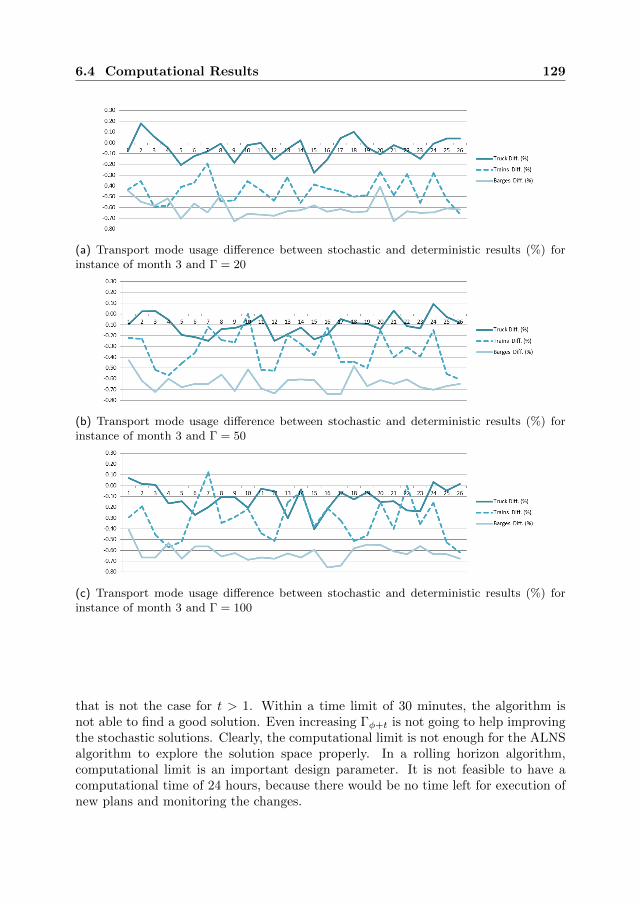
6.4 Computational Results 129
(a) Transport mode usage difference between stochastic and deterministic results (%) forinstance of month 3 and Γ = 20
(b) Transport mode usage difference between stochastic and deterministic results (%) forinstance of month 3 and Γ = 50
(c) Transport mode usage difference between stochastic and deterministic results (%) forinstance of month 3 and Γ = 100
that is not the case for t > 1. Within a time limit of 30 minutes, the algorithm isnot able to find a good solution. Even increasing Γφ+t is not going to help improvingthe stochastic solutions. Clearly, the computational limit is not enough for the ALNSalgorithm to explore the solution space properly. In a rolling horizon algorithm,computational limit is an important design parameter. It is not feasible to have acomputational time of 24 hours, because there would be no time left for execution ofnew plans and monitoring the changes.

130 Chapter 6. A Scenario-based Rolling Horizon with Uncertain Demand
Table 6.2 Comparison of multi-roll scenario population
n month t Γφ+1 Γφ+2 Γφ+3
RollDeter.Costs
A.D.(%)
RollDeter.Sim.Costs
A.D.(%)
TotalDeter.Costs
A.D.(%)
TotalStoch.Costs.
A.D.(%)
Avg.Cost
Diff. (%)
Rollswith
WorseStoch.
Sol. (%)
20 1 1 100 - - 1,119,738 1.00 596,139 0.80 1,715,877 1.10 1,429,859 0.68 -13.55 1920 1 2 20 20 - 4,783,234 4.33 1,659,446 4.76 5,442,680 4.40 6,512,272 10.30 91.10 5720 1 3 20 10 5 5,721,009 6.79 1,389,983 5.94 6,110,992 5.62 8,365,953 13.46 100.75 80
6.5 Conclusions
To have smarter day-to-day transportation plans, incorporating the available informa-tion of today might not enough. Having an anticipation of what future imposes, mighthelp in avoiding shortage of mode capacity, and extra costs of last-minute renting oroutsourcing. In perishable supply chains, uncertainty of demand and the pressureto deliver the customer demand in time and with the required freshness, motivatescontemplating the aftermath of this uncertainty into the operational planning.
This chapter incorporated uncertainty of demand into the operational planning ofmultimodal transportation of perishable products. The rolling horizon framework ofthe previous chapter was extended, to embed a truncated Scenario-based Two-stageStochastic Program (STSP), which is periodically solved. At the first stage of theSTSP, the fleet arrangement and all forward and backward RTI flows of realized ordersare planned, and at the second stage, this arrangement and the remaining capacityand resources are used to provide optimal product flow and RTI repositioning, for agenerated set of scenarios. For analysis purposes, the framework hosts two parallelplanning tracks, one for the stochastic transportation planning and one for thedeterministic one. Two ALNS algorithms with new and redesigned operators, andnew parameter tuning solve them, after which a simulation module is called in orderto analyze performance of the deterministic solutions on the scenario population.
The new rolling horizon algorithm was tested on three sets of instances, representingdaily demand of 20 location over 3 months. In overall, results show that stochasticsolutions are on average cheaper than the deterministic solution, which proves theimportance of including demand uncertainty into the planning.
The size of scenario population and the number of future rolls that these scenariosare picked from, are key factors in the performance of the ALNS algorithm. Scenariopopulation can be generated based on daily demand distribution of the next day, thenext two days, and the next three days. For the first case, bigger population size 100has the best performance based on both costs and the number of rolls with worsestochastic solutions. In addition, with bigger population, more truck transportationare replaced by trains. For the cases with multi-roll scenario generation, results showthat the ALNS is not able to get good solutions within 30 minutes and in using amulti-roll strategy, the computational time limit should be significantly longer.
One future work can be to include other types of uncertainty sources into the planning,
6.5 Conclusions 131
such as network disruption sources, i.e. travel cancellations, accidents, and delays.Another future research possibility is to find strategies to handle multi-roll scenariopopulations in the STSP of the framework. The more future is anticipated, thesmarter and smoother day-to-day transportation might get.

132 Chapter 6. A Scenario-based Rolling Horizon with Uncertain Demand

Part IV
Closing


Chapter 7
Conclusions
Multimodal transportation has long been proven to offer a potential platform fora more efficient, reliable, flexible, and sustainable freight transportation. Forperishable product industries, such as the horticultural industry of the Netherlands,the opportunities and the threads of transporting their products via a multimodalplatform is still under study.
Perishable products have short shelf life, and if not appropriately stored or trans-ported, they lose their value over time. Improved temperature-controlled containertechnologies will facilitate transition of transporting these products from fast,expensive, and environmentally undesirable road and air transport, to cheaper andmore environmentally friendly rail and waterway ones. However, there are certainquestions that should be answered: “what modes can be used to transport theseproducts? when should they be transported? what are the economic gains? andwhat does a flexible transportation plan capable of responding to day-to-day operationdynamics and uncertainties look like?”
Planning a multimodal transportation added to the extra product preservationrequirements of perishable products, is heavily complex, and requires tailored models,policies, and tools. The goal of this thesis is to develop relevant models and algorithmsfor multimodal transportation planning of perishable products. Chapter 1 first pointedout the motivations and challenges of this thesis. Next, it gave an overview of theliterature on planning transportation of perishable products, and showed that theliterature on long-haul transportation of these products, and explicitly on modelingtemperature-based quality measures, is very limited. Accordingly, it then defined thescope of the thesis, and introduced the research objectives addressed in it.
Assuming that a multimodal infrastructure and proper quality preservation technolo-gies are present, this thesis was divided into two parts, dedicated to studying tacticalplanning and operational planning. Chapter 2 gave an overview of the recent research

136 Chapter 7. Conclusions
on tactical and operational planning problems of multimodal freight transportation,by looking at their motivations, the characteristics of the different encounteredproblems, and their respective solution methods. This chapter highlighted a gap inmultimodal transportation planning of perishable products, and suggested integratingthe network planning and the management of assets such as Returnable TransportItems (RTIs), as well as contemplating dynamicity and stochasticity of differentaspects of these planning problems.
This thesis builds upon this literature and defines four research objectives in the areaof tactical and operational planning.
7.1 Tactical Planning
The first step to plan multimodal transportation of perishable products is tounderstand its dynamics and translate them into measurable values and tangiblerelations. Therefore, the first research objective is:
Research Objective 1: Model the multimodal transportation planning problem andpropose a mathematical formulation to optimize it. In modeling the multimodal trans-portation planning with perishable products and management of RTIs, measuringthe product quality and preserving the quality should be addressed. In addition,characteristics of different transportation modes, regarding their scheduling, theircapacity, etc. should be contemplated, and finally, the flow, repositioning, and balanceof the RTIs used for transporting products should be included.
For this objective, Chapter 3 defined this planning problem, and modeled it asa Mixed-Integer Program (MIP), which is an extension of Fixed-cost CapacitatedMulticommodity Network Flow Problems (FCMNFP). New sets of constraints wereadded to the classic FCMNFP. These constraints include a product quality measurebased on temperature and travel time, and enforce a maximum limit on products,after which they are considered perished. Moreover, the forward flow of loaded RTIswas integrated with the backward flow of empty ones via a set of novel constraints.Based on RTI demands, these constraints assign and move the needed empty ones. Intotal, the model was tested on 21 instances with different number of locations, up to 3transportation modes, and up to 50 randomly generated orders. The problem is large,because of huge matrices. Some computational tactics were used to help decreasingthe time and memory issues related to their dimensions. However, solving instanceswith 50 orders and more by a state-of-the-art MIP solver is impossible. Due to severecomplexity, the problem of Chapter 3 included only one size of RTI (e.g. trolleys),however, in transporting perishable products, there are different types and sizes ofRTIs. In an attempt, Appendix A later extended the proposed MIP to include three(small, medium, and large) sizes of RTIs, where each size of RTIs should be loaded(or nested) into its immediate bigger RTI size in order to be transported. In practicefor instance, buckets and boxes are loaded onto trolleys, and trolleys later are loaded

7.2 Operational Planning 137
into containers. The extended MIP was also computationally tested and verified.The results showed that a state-of-the-art MIP solver is hardly able to find optimalsolutions for even the smallest instances with 5 orders within 10 hours. Therefore,solving real-world sizes of such a planning problem to optimality is impossible.
The dimension and complexity of the problem in Chapter 3 clearly confines its abilityto find optimal solutions for the real-world case. Therefore, the second researchobjective is:
Research Objective 2: Develop an algorithm for multimodal transportation plan-ning and resource management of perishable products. This algorithm should providegood solutions within reasonable computational time, considering all constraints andrequirements of the planning problem modeled above.
For this objective, Chapter 4 proposed a solution algorithm, which is an adaptation ofthe classic Adaptive Large Neighborhood Search (ALNS) algorithm. New path-basedneighborhoods were introduced to the algorithm, which at each iteration, work onvarious combinations of orders. Furthermore, specific scoring was used to manage thecomputation time of the algorithm, and neighborhood-based Tabu lists were added toimprove the search. A diversification step was also added to exploit unvisited partsof the solution space. The proposed algorithm was tested on instances of Chapter 3,where it showed robustness and good performance. The algorithm is relatively fast,does not take up much memory, and provides good and robust solutions. It was evenable to find solutions for the instances which the MIP solver was not able to find anysolution for.
7.2 Operational Planning
Tactical planning tools alone are not sufficient for the day-to-day management ofoperations. A transportation system is constantly changing from one day to thenext, and the dynamics of these changes require different decisions to be made, moredetailed factors to include, and probably different objectives to consider. Thereforethe next research objective is:
Research Objective 3: Develop a framework for operational planning of multimodaltransportation with perishable products and management of RTIs. This frameworkshould take the day-to-day changes of the system into account, and based on theinformation it receives and its observation of the system evolution, provide efficientactions and adjustments.
For this objective, Chapter 5 first defined this planning problem, which is a dynamicextension to the planning problem of Chapter 3. In this planning problem, at specificdecision occasions (e.g. every 12 hours) and based on collected data on arriveddemand and system evolution, a deterministic FCMNFP with updated parameterson new demand, RTI repositioning, and available multimodal transportation options,

138 Chapter 7. Conclusions
is reformulated and solved. This chapter then proposed a rolling-horizon framework,where a modified version of the ALNS of Chapter 4 is employed to provide new andadjusted plans in response to the dynamics of day-to-day operations. This frameworkwas tested on three instances, set over the course of 3 months, and with varioussettings. The results highlighted what role each setting (e.g. the length of a roll)plays in the operational planning.
This framework only relies on available information, representing what demandhas already been revealed and what has already happened upto a certain decisionoccasion, and does not have any view or anticipation of the future. Therefore,the day-to-day solutions might not provide efficient plans which can also respondto unforeseen situations such as demand fluctuations. Nevertheless, there is historicaldata available on demand, supply, and availability of transportation modes. Thisdata can provide further insights and perception about future scenarios, especially oncustomer demand. Therefore, the final objective is:
Research Objective 4: Model anticipation of future demand and incorporate it in thedeveloped operational planning framework. Even though demand is uncertain, thereis historical data available on its behavior. Based on the insights this data providesabout future demand scenarios, the modified framework should take different actions,offering a smarter and more flexible transportation.
For this objective, the deterministic FCMNFP problem of Chapter 5 was extended toinclude stochastic demand, and was modeled as a Scenario-based Two-stage StochasticProgram (STSP), where at the first stage and besides planning the realized demand,the multimodal fleet is arranged and at the second stage, this arrangement is used tofind optimal product flow and RTI repositioning over a generated set of scenarios. Therolling-horizon framework of Chapter 5 is further extended to include these scenarios,and its ALNS algorithm is also modified to include redesigned neighborhoods andparameter tuning. As a result, at the end of each roll, new data is collected, and aftergenerating a scenario population, the STSP is solved, and new plans and adjustmentsare made. The framework hosts two parallel planning tracks, one for the stochasticFCMNFP and one for the deterministic one. A simulation module is used to comparethe performance of the deterministic solutions with the stochastic ones.
The new rolling horizon framework was tested on three sets of instances, with dailydemand distribution of 20 locations over 3 months. Results show that stochasticsolutions are on average cheaper than the deterministic solution which proves theimportance of including anticipation of future demand into the planning. Moreover,the size of scenario population and the number of future rolls that these scenarios arepicked from, were shown to be key factors in the performance of the ALNS algorithm.

7.3 Managerial Insights 139
7.3 Managerial Insights
Depending on the characteristics of a perishable product, its quality, and its market,different tactical and operational planning problems are formulated, and therefore,different tactical and operational solutions are obtained.
This thesis used the Europe-wide transportation of highly perishable horticulturalproducts with their time-temperature quality measure for its experiments andverifications. It assumed to have 20 hub locations, with RTIs stored at two of them. Anetwork of Trans-European Transport (TEN-T) with three modes of truck, train, andbarge was assumed to be available, and the sale reports of 2013 was used to generatethe set of transport orders. The proposed models and algorithms in this thesisare however capable of adapting to any type of perishable product transportationnetwork, with any combination of modes, RTI storage locations, cost structure, qualitymeasures, and transport orders. Moreover, the following general insights are drawn:
In Part II, results show that an integrated planning of transporting products andrepositioning the RTIs provides much cheaper transportation plans. The delivery duedates and the hard vaselife restriction of products however, do not allow for muchusage of non-truck modes in forward flows of products. Trains and barges are mostlyused for repositioning of RTIs. Timely repositioning of empty RTIs is essential and noRTI of any type and size is an exception. Results show that having a central storagefor all of them, close to the hubs with highest forward flow traffic results in significantrepositioning savings.
In Part III, results show that in designing a good operational planning framework,the time intervals between consecutive decision epochs are the key in the trade-offbetween operational costs and loss of sale. The shorter planning intervals are (e.g.every six hours), the less sale is lost. However, shorter intervals come with the priceof having less information about the future. With less information, the chances ofconsolidation decrease, and the arranged fleet become expensive. This problem issolved by incorporating an anticipation of the future. In this thesis, future demandwith its daily and weekly trends was taken into account, and by analyzing historicaldata and trends, scenarios representing their possibilities were generated. The resultsshow that including future demand scenarios into the operational planning offerssmarter and more efficient fleet arrangement. Such plans provide a flexibility totackle future demand fluctuations. There is however a trade-off between how manyscenarios are defined and how much time is allowed for computations. It is desirableto define as many scenarios as possible, but the computational limits might not allowfinding good plans.
7.4 Future Research Suggestions
140 Chapter 7. Conclusions
The first future research possibility is to study tactical and operational planningof perishable products with other temperature regimes and quality preservationrestrictions. Each industry has its own measures and even quality decay penalties,and it would be interesting to study the structure of solutions with these restrictions.
Moreover, in this thesis, it was assumed that products are compatible and theycan be consolidated into similar temperature controlled modes and containers. Inpractice, perishable industries might share and combine their logistics to benefit fromeconomy of scale. In such a setting, each product has its own quality preservationrequirement, and its preservation regime might not be compatible with others.Moreover, the objectives of the cooperating industries might not be congruent. Hence,extra constraints and multiple objectives are needed for the combined long-haultransportation planning.
In this thesis, the family of ALNS metaheuristics were used to design the solutionalgorithms. These algorithms have shown great performance in solving large scaleVehicle Routing Problems (VRP), and this thesis adapted them to the family ofFixed-charge Capacitated Multicommodity Network Flow Problems (FCMNFP). Afuture research suggestion is to study strategies that would enhance their performancein solving large scale FCMNFP problems even further.
Management of multi-size loading units is new to the literature, opening a majoropportunity for more research on its modeling as well as solution design. In thisthesis, a model was proposed for a transportation problem with three sizes of RTIsand their loading relations, and it was shown that it is a very complex problem. Aninteresting future research would be to find models and solution algorithms that canhandle the relations between different sizes and types of such loading units, and forpractical cases.
In operational planning, a future work possibility is to include other types ofuncertainty sources into the planning. The examples are uncertainty of service time athubs, network disruption sources (such as travel cancellations, accidents, and delays),and availability of modes.

Appendix A
An Extended MIP forMultimodal FCMNFP withPerishable Products andEmpty Repositioning ofThree Sizes
Chapter 3 proposed a Mixed-Integer Program (MIP) for the multimodal transporta-tion of perishable products with integrated management of Returnable TransportItems (RTIs). In that chapter, RTIs were assumed to have equal sizes, or in otherwords, they were homogeneous. In a perishable industry however, RTIs can havedifferent sizes ranging from a small box to a large 45-feet container. This technicalappendix presents a model for multimodal transportation with three sizes of RTI. Thecontribution of this work is to include the interactions between these classes of RTIs(such as their loading hierarchy) into the model of Chapter 3. Sections A.1 and A.2describe the problem and the related literature respectively. Sections A.3 and A.4then, explain the extensions to the previous model, and present the mathematicalformulation respectively. Section 3.5 shows the results of solving this problem bya state-of-the-art MIP solver. Finally, in Section A.6, some concluding remarks areprovided.

142 Chapter A. An Extended MIP with Empty Repositioning of Three Sizes
Figure A.1 Floricultural multi-size RTI logistics
A.1 Problem Description
Tactical planning deals with utilizing a given transportation infrastructure andmanagement of all the assets (here, RTIs) involved. RTIs can have different sizesranging from a small box to a large 45-feet container. In the horticultural industryof the Netherlands for instance, flowers and bouquets are loaded in small RTIs(e.g. boxes and buckets) and small RTIs are then loaded onto medium RTIs (e.g.cages, Dense fusters, staple wagons, trolleys; Figure A.1). Chapter 3 emphasizedthe importance of timely repositioning of empty RTIs, and no RTI of any size isan exception. Their number is limited, and their availability plays a crucial role indecreasing handling times and preserving the product quality.
Multi-size asset management in essence is unique, and different from some of thestate-of-the-art heterogeneous fleet management problems (such as in Baldacci et al.[2010]). Heterogeneous fleet or in general assets, have more than one type, each withits own capacity, costs, and some other distinct characteristics. A multimodal fleetcan be viewed as a special case of a heterogeneous fleet. However, these assets are notloaded into (onto) each other. This phenomenon is here called the loading hierarchy.
Loading hierarchy brings extra features to the model. In perishable long-haultransportation for example: 1) Small RTIs are loaded onto medium ones if transportedby trucks, 2) Medium RTIs are then loaded into big RTIs if transported by trains orbarges (Figure A.2). 3) Capacity of medium and big RTIs is defined by the number ofsmaller ones they can carry, and capacity of transport modes is defined based on thenumber of biggest RTIs they can accommodate. 4) Bigger RTIs also have a storagelocation, and finally, 5) unlike small RTIs, medium and big ones are labeled, whichenables tracking the orders that are consolidated and carried in each of them.

A.1 Problem Description 143
Figure A.2 Resource allocation structure in a long-haul transportation system
(a) Nesting (b) Folding
Figure A.3 Empty nesting and folding
Besides these new features, a nesting ratio is also introduced to the multi-size RTIproblem. Nesting ratio is the average ratio of space occupied by an empty RTIcompared to a full one. Figures A.3a and A.3b show how much space nesting orfolding RTIs can save. For instance, if a loaded trolley takes on average one unit ofspace, its empty one takes on average 0.3 unit of space. This ratio is then used inrelated capacity constraints. Folding or nesting empty RTIs help more consolidation,less usage of transport modes, and therefore, a cheaper repositioning operation.
One of the biggest challenges of this problem is synchronization of operations for allRTI sizes. To pick up a transportation order, all required RTIs should be availablein time based on their loading hierarchy, and their operations cannot be segregated.For example, medium RTIs cannot start loading, if small RTIs have not arrived tothe pickup location and are ready.
The main decisions in this problem are the flow of products (customer demand), therepositioning of RTIs (now for all sizes), and the selection of transport modes and

144 Chapter A. An Extended MIP with Empty Repositioning of Three Sizes
schedules to do these jobs. Similar to Chapter 3, the main decisions are based onthe flow of RTIs. Their number throughout the network is limited and their flow issubjected to strict resource balance constraints. For instance, the number of RTIsavailable at the beginning of the planning horizon should be equal to their number atthe end of horizon.
Demand is represented by orders, which have their own pair of origin and destinationlocations, its volume, pickup and delivery schedules, and freshness requirements (amaximum Time Temperature Sum (TTS) limit). However, the order volume nowshows the number of small RTIs (e.g. 32 buckets) needed to transport products. Theproducts can be picked up and loaded onto the RTIs at an earliest given time, andshould be delivered to the destination and unloaded at an latest given time.
In order to transport full and empty RTIs, fleets of different transportation modesare available throughout the network, each with its given schedules, its specifictemperature, capacity (here, based on the biggest RTI they can accommodate), andavailable number of vehicles. Locations also have their own temperature, which isincluded in the quality measure of loading, unloading, and holding of laden RTIs atthese locations.
The objective function of this problem, similar to Chapter 3, is to minimize totalsystem costs, including costs related to employment of modes, costs of handling andstoring RTIs, administrative costs of these operations, etc.
A.2 Related Literature
The literature on heterogeneous asset management is vast. As stated earlier, the entiremultimodal transportation planning literature can be considered as a subdivision ofheterogeneous asset management literature.
Baldacci et al. [2010] and Topaloglu and Powell [2006] are two explicit examples.Baldacci et al. [2010] provide an overview of different variants of heterogeneous vehiclerouting problems (VRPs), and discuss presented solution approaches in the literature.Topaloglu and Powell [2006] models a heterogeneous fleet management problem andthe substitution among them as a Approximate Dynamic Program (ADP).
The problem of this chapter is an extension to the classic Fixed-charge CapacitatedMulticommodity Network Flow Problem (FCMNFP), where additional sets ofconstraints related to product quality preservation and management of heterogeneousReturnable Transport Items (RTI), are added to these problems.
Combined planning of different assets with their complex interactions is modeled vialayering [Powell, 2003], therefore, a multi-size RTI FCMNFP can be formulated asa multi-layer MIP. The closest study to this environment is Zhu et al. [2014]. Theystudy a rail transportation problem where customer demand comes to the system as
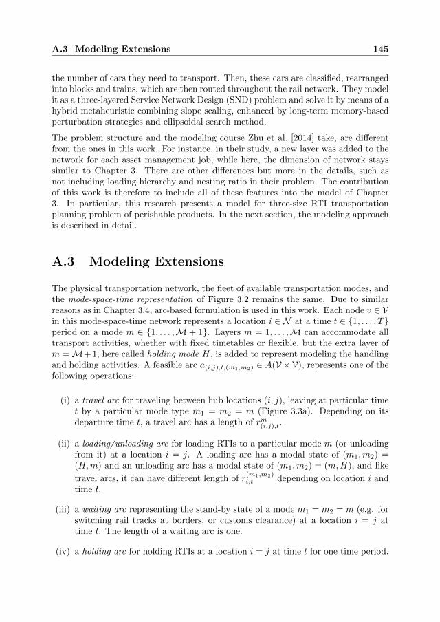
A.3 Modeling Extensions 145
the number of cars they need to transport. Then, these cars are classified, rearrangedinto blocks and trains, which are then routed throughout the rail network. They modelit as a three-layered Service Network Design (SND) problem and solve it by means of ahybrid metaheuristic combining slope scaling, enhanced by long-term memory-basedperturbation strategies and ellipsoidal search method.
The problem structure and the modeling course Zhu et al. [2014] take, are differentfrom the ones in this work. For instance, in their study, a new layer was added to thenetwork for each asset management job, while here, the dimension of network stayssimilar to Chapter 3. There are other differences but more in the details, such asnot including loading hierarchy and nesting ratio in their problem. The contributionof this work is therefore to include all of these features into the model of Chapter3. In particular, this research presents a model for three-size RTI transportationplanning problem of perishable products. In the next section, the modeling approachis described in detail.
A.3 Modeling Extensions
The physical transportation network, the fleet of available transportation modes, andthe mode-space-time representation of Figure 3.2 remains the same. Due to similarreasons as in Chapter 3.4, arc-based formulation is used in this work. Each node v ∈ Vin this mode-space-time network represents a location i ∈ N at a time t ∈ {1, . . . , T}period on a mode m ∈ {1, . . . ,M + 1}. Layers m = 1, . . . ,M can accommodate alltransport activities, whether with fixed timetables or flexible, but the extra layer ofm =M+1, here called holding mode H, is added to represent modeling the handlingand holding activities. A feasible arc a(i,j),t,(m1,m2) ∈ A(V ×V), represents one of thefollowing operations:
(i) a travel arc for traveling between hub locations (i, j), leaving at particular timet by a particular mode type m1 = m2 = m (Figure 3.3a). Depending on itsdeparture time t, a travel arc has a length of rm(i,j),t.
(ii) a loading/unloading arc for loading RTIs to a particular mode m (or unloadingfrom it) at a location i = j. A loading arc has a modal state of (m1,m2) =(H,m) and an unloading arc has a modal state of (m1,m2) = (m,H), and like
travel arcs, it can have different length of r(m1,m2)i,t depending on location i and
time t.
(iii) a waiting arc representing the stand-by state of a mode m1 = m2 = m (e.g. forswitching rail tracks at borders, or customs clearance) at a location i = j attime t. The length of a waiting arc is one.
(iv) a holding arc for holding RTIs at a location i = j at time t for one time period.

146 Chapter A. An Extended MIP with Empty Repositioning of Three Sizes
Since the last three activities occur at the locations, the arcs representing them arecalled location arcs (Figure 3.3b). Let A1 = {a(i,j),t,(m1,m2) ∈ A(V × V) | i 6= j,m1 =m2} be the set of all feasible and given travel arcs in the mode-space-time network,and let A2 = {a(i,j),t,(m1,m2) ∈ A(V × V) | i = j,m1 = H ‖ m2 = H} be the setof all feasible location arcs in the network. Similarly, let Am = {a(i,j),t,(m1,m2) ∈A(V ×V) | m1 = H ‖ m2 = H} be the set of all feasible loading, unloading, traveling,and waiting arcs in the network related to mode m.
In this three-size RTI problem, there are three sets of small, medi, and big RTIs.Therefore, the decisions are now:
1. small laden flow decisions for loaded small RTIs that are transporting theproducts,
2. small assign flow decisions for empty small RTIs that are repositioned from alocation with surplus of RTIs, to the origin locations of orders to be assigned totheir transport,
3. small repos flow decisions for empty small RTIs that are repositioned from thedestination locations of orders back to the storage locations with RTI shortage.
4. medi usage decisions for each available medium RTI, which is equal to 1, ifa particular medium RTI is used to pickup and deliver the small RTIs flowedaround the network, and is equal to 0, otherwise,
5. big usage decisions for each available big RTI, which is equal to 1, if a particularbig RTI is used to pickup and deliver the medium RTIs flowed around thenetwork, and is equal to 0, otherwise.
Decisions on small RTIs are different from the decisions on medium and big RTIs.Small RTIs are not unique (labeled) and have a nonnegative nature, while mediumand big RTIs are labeled, and usage and routing of each of them is optimized in thisplanning problem. Therefore, their decision variables have a binary nature.
In the remainder of this section, the proposed MIP is presented. Appendix B providesa summary of all notations used.
A.4 A Mathematical Model for RTIs with ThreeSizes
In this section, the mathematical formulation for the multimodal network flowproblem with product quality preservation and RTI management of three sizes isexplained.

A.4 A Mathematical Model for RTIs with Three Sizes 147
An order p is characterized by its origin O(p), its destination D(p), volume (basedon small RTIs) wp, an earliest pickup time of PT (p), a latest delivery due date ofDT (p), and the maximum allowed TTS of Lp. The number of needed medium andbig RTIs is not indicated in the order. Their usage and routing are decisions that themodel will determine based on all consolidation options and order requirements.
Again a fleet of m ∈ {1, . . . ,M} transportation modes with their own capacity, speed,fixed costs, and variable costs is available. However, capacity and variable costs ofeach mode are now defined on medium and big RTI scale. In general, if transportationmodes have their own installed big containers (e.g. truck trailers, train cars, etc.),their capacity is defined on the number of medium RTIs they can accommodate(Figure A.2). Otherwise, their capacity is based on big RTIs. In Chapter 3, trucks,trains, and barges were the possible modes. Here, trucks are replaced with reefertrucks. Since, they not to be able to carry containers, their capacity is defined bythe number of medium RTIs they can carry. Such an assumption makes the MIP aspecial case and adds to the complexity of the problem, but it is not unrealistic. Thereason is to show how these capacity differences can be represented in a MIP.
Each location i is assumed to have a temperature li,t at time t. Moreover, eachlocation i is assumed to have Si,small, Si,medi, Si,big ≥ 0 number of small, medium,and big RTIs available at the beginning of the planning horizon, and the number ofRTIs at the end of horizon should be equal to the initial value. Of course, the locationof small, medium, and big RTI storages are not necessarily the same, and inbound
hubs are not obliged to keep similar number of them. Let C(m1,m2)i,small , C
(m1,m2)i,medi , and
C(m1,m2)i,big be the general term for loading, unloading, and holding costs per small,
medium, and big RTI per time period, which are enforced on the location arcs.
Similar to Chapter 3, for each flow decision laden, assign, or repos, two sets of decisionvariables are defined: 1) x to show how many RTIs enter an arc a(i,j),t,(m1,m2), and2) x to show how many RTIs exit the arc. Similarly, there are two sets of variablesy and y to show the number of vehicles respectively entering and exiting an arc.The auxiliary binary variables b and b are also added to help calculating TTS. Threecategories of variables U track the inbound and outbound small flows at each locationand to connect the flow of loaded and empty small RTIs throughout the network.The auxiliary binary variables b and b help calculating Time Temperature Sum (TTS)measure which is used as a quality preservation constraint.
As mentioned in Section A.1, medium and big RTIs are labeled, meaning that theusage and routing of each of them is optimized in the model. Assuming g = 1, . . . ,Gand k = 1, . . . ,K number of medium and big RTIs available in the system, new setsof binary variables are introduced showing their usage. Two sets of variables eg, ekshow a medium and a big RTI entering an arc, and two sets of variables eg and ekshow a medium and a big RTI exiting the arc. When a medium and a big RTI areused to move small RTIs between locations i, and j, departing at time t, their usagevariables are equal to 1. Similar to small RTIs, there are variables Ug and Uk to track

148 Chapter A. An Extended MIP with Empty Repositioning of Three Sizes
Figure A.4 A Simplified Example Showing Small RTI flows in comparison of mediumand big RTI Usage
the inbound and outbound medium and big RTI usage throughout the network.
To give an example of how these variables are connected to each other, Figure A.4shows an order for transporting small RTIs from location 3 to location 4 departingat t3. For this order, empty small RTIs are assigned from their storage at location 2and later, repositioned back to this location. In order to transport these small RTIs,container k picks up trolley g and goes to the location where small RTIs are going tobe transported. After finishing its transportation tasks, container k delivers trolley gback to its storage location at 1. Of course, this is a simplified example, and there aremany x, b, eg, and ek variables, as well as y variables that become positive in such acase.
A value G for the total number of available medium RTIs is assumed in the problem.It is a given, but in this work, assuming capg to be the capacity of medium RTIsbased on the number of small ones they can carry, this value is set to:
G =
⌈∑Pp=1 wp
capg
⌉+ P (A–1)
Likewise, the total number of available big RTIs is K, and assuming their capacity tobe capk equal to the number of medium RTIs they can accommodate, its value is seta priori to:
K =
⌈ ∑Pp=1 wp
capg × capk
⌉+ P (A–2)
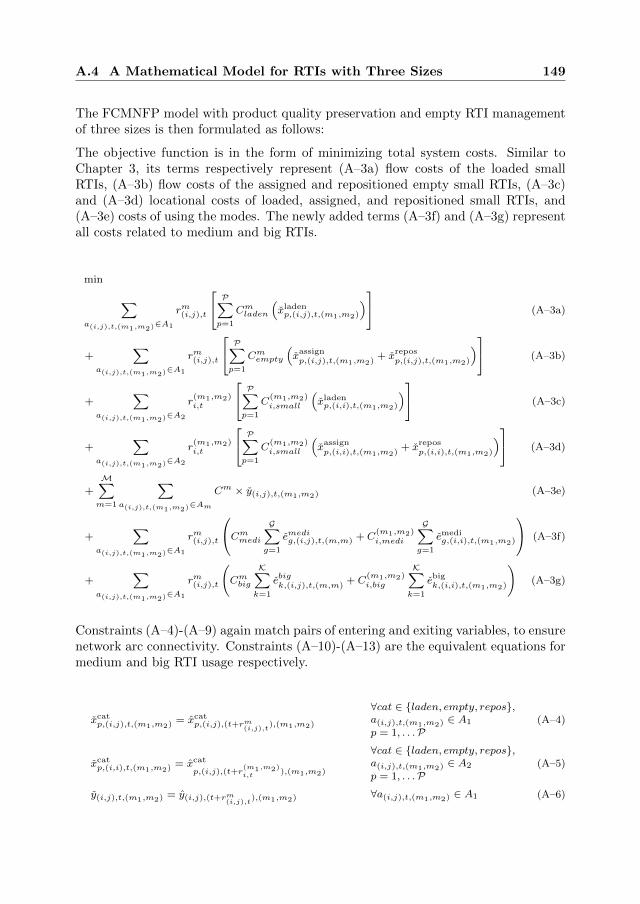
A.4 A Mathematical Model for RTIs with Three Sizes 149
The FCMNFP model with product quality preservation and empty RTI managementof three sizes is then formulated as follows:
The objective function is in the form of minimizing total system costs. Similar toChapter 3, its terms respectively represent (A–3a) flow costs of the loaded smallRTIs, (A–3b) flow costs of the assigned and repositioned empty small RTIs, (A–3c)and (A–3d) locational costs of loaded, assigned, and repositioned small RTIs, and(A–3e) costs of using the modes. The newly added terms (A–3f) and (A–3g) representall costs related to medium and big RTIs.
min
∑a(i,j),t,(m1,m2)∈A1
rm(i,j),t
P∑p=1
Cmladen
(xladenp,(i,j),t,(m1,m2)
) (A–3a)
+∑
a(i,j),t,(m1,m2)∈A1
rm(i,j),t
P∑p=1
Cmempty
(xassignp,(i,j),t,(m1,m2)
+ xreposp,(i,j),t,(m1,m2)
) (A–3b)
+∑
a(i,j),t,(m1,m2)∈A2
r(m1,m2)i,t
P∑p=1
C(m1,m2)i,small
(xladenp,(i,i),t,(m1,m2)
) (A–3c)
+∑
a(i,j),t,(m1,m2)∈A2
r(m1,m2)i,t
P∑p=1
C(m1,m2)i,small
(xassignp,(i,i),t,(m1,m2)
+ xreposp,(i,i),t,(m1,m2)
) (A–3d)
+
M∑m=1
∑a(i,j),t,(m1,m2)∈Am
Cm × y(i,j),t,(m1,m2) (A–3e)
+∑
a(i,j),t,(m1,m2)∈A1
rm(i,j),t
Cmmedi G∑g=1
emedig,(i,j),t,(m,m) + C(m1,m2)i,medi
G∑g=1
emedig,(i,i),t,(m1,m2)
(A–3f)
+∑
a(i,j),t,(m1,m2)∈A1
rm(i,j),t
(Cmbig
K∑k=1
ebigk,(i,j),t,(m,m)
+ C(m1,m2)i,big
K∑k=1
ebigk,(i,i),t,(m1,m2)
)(A–3g)
Constraints (A–4)-(A–9) again match pairs of entering and exiting variables, to ensurenetwork arc connectivity. Constraints (A–10)-(A–13) are the equivalent equations formedium and big RTI usage respectively.
xcatp,(i,j),t,(m1,m2) = xcat
p,(i,j),(t+rm(i,j),t
),(m1,m2)
∀cat ∈ {laden, empty, repos},a(i,j),t,(m1,m2) ∈ A1
p = 1, . . .P(A–4)
xcatp,(i,i),t,(m1,m2) = xcat
p,(i,j),(t+r(m1,m2)i,t ),(m1,m2)
∀cat ∈ {laden, empty, repos},a(i,j),t,(m1,m2) ∈ A2
p = 1, . . .P(A–5)
y(i,j),t,(m1,m2) = y(i,j),(t+rm(i,j),t
),(m1,m2) ∀a(i,j),t,(m1,m2) ∈ A1 (A–6)
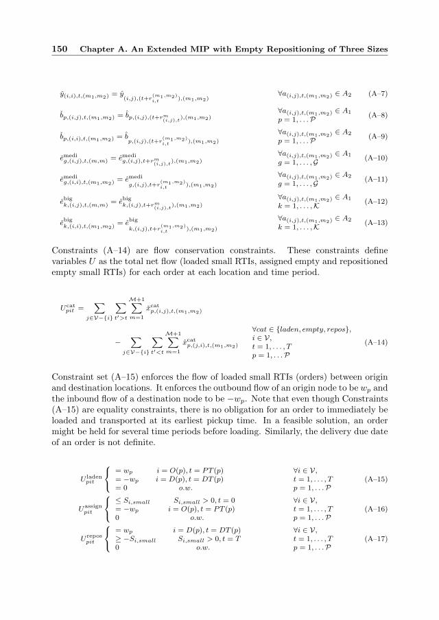
150 Chapter A. An Extended MIP with Empty Repositioning of Three Sizes
y(i,i),t,(m1,m2) = y(i,j),(t+r
(m1,m2)i,t ),(m1,m2)
∀a(i,j),t,(m1,m2) ∈ A2 (A–7)
bp,(i,j),t,(m1,m2) = bp,(i,j),(t+rm(i,j),t
),(m1,m2)∀a(i,j),t,(m1,m2) ∈ A1
p = 1, . . .P (A–8)
bp,(i,i),t,(m1,m2) = bp,(i,j),(t+r
(m1,m2)i,t ),(m1,m2)
∀a(i,j),t,(m1,m2) ∈ A2
p = 1, . . .P (A–9)
emedig,(i,j),t,(m,m) = emedi
g,(i,j),t+rm(i,j),t
),(m1,m2)
∀a(i,j),t,(m1,m2) ∈ A1
g = 1, . . . ,G (A–10)
emedig,(i,i),t,(m1,m2) = emedi
g,(i,j),t+r(m1,m2)i,t ),(m1,m2)
∀a(i,j),t,(m1,m2) ∈ A2
g = 1, . . . ,G (A–11)
ebigk,(i,j),t,(m,m)
= ebigk,(i,j),t+rm
(i,j),t),(m1,m2)
∀a(i,j),t,(m1,m2) ∈ A1
k = 1, . . . ,K (A–12)
ebigk,(i,i),t,(m1,m2)
= ebig
k,(i,j),t+r(m1,m2)i,t ),(m1,m2)
∀a(i,j),t,(m1,m2) ∈ A2
k = 1, . . . ,K (A–13)
Constraints (A–14) are flow conservation constraints. These constraints definevariables U as the total net flow (loaded small RTIs, assigned empty and repositionedempty small RTIs) for each order at each location and time period.
Ucatpit =
∑j∈V−{i}
∑t′>t
M+1∑m=1
xcatp,(i,j),t,(m1,m2)
−∑
j∈V−{i}
∑t′<t
M+1∑m=1
xcatp,(j,i),t,(m1,m2)
∀cat ∈ {laden, empty, repos},i ∈ V,t = 1, . . . , Tp = 1, . . .P
(A–14)
Constraint set (A–15) enforces the flow of loaded small RTIs (orders) between originand destination locations. It enforces the outbound flow of an origin node to be wp andthe inbound flow of a destination node to be −wp. Note that even though Constraints(A–15) are equality constraints, there is no obligation for an order to immediately beloaded and transported at its earliest pickup time. In a feasible solution, an ordermight be held for several time periods before loading. Similarly, the delivery due dateof an order is not definite.
U ladenpit
= wp i = O(p), t = PT (p)= −wp i = D(p), t = DT (p)= 0 o.w.
∀i ∈ V,t = 1, . . . , Tp = 1, . . .P
(A–15)
Uassignpit
≤ Si,small Si,small > 0, t = 0= −wp i = O(p), t = PT (p)0 o.w.
∀i ∈ V,t = 1, . . . , Tp = 1, . . .P
(A–16)
Urepospit
= wp i = D(p), t = DT (p)≥ −Si,small Si,small > 0, t = T0 o.w.
∀i ∈ V,t = 1, . . . , Tp = 1, . . .P
(A–17)

A.4 A Mathematical Model for RTIs with Three Sizes 151
Constraints (A–16) and (A–17), in a similar fashion enforce the flow of empty smallRTIs between origin and destination locations. The origin locations of the assignedempty RTIs are the RTI storage locations with Si,small > 0. Their destinationlocations are the locations where they are needed to be loaded and transport theproducts (O(p),PT(p)). On the other hand, the repositioned empty RTIs need to getback to the storage locations. Therefore, the locations with Si,small > 0 are theirdestinations and their origin locations are the locations where the loaded RTIs areunloaded (D(p),DT(p)). Constraint (A–18) enforces the number of empty small RTIsassigned from a storage locations to be equal to the number of RTIs returned there.
∑j∈V−{i}
M+1∑m=1
P∑p=1
xassignp,(i,j),0,(m1,m2)
=∑
j∈V−{i}
M+1∑m=1
P∑p=1
xreposp,(j,i),T,(m1,m2)
∀i ∈ V : Si > 0
(A–18)
Constraints (A–19) and (A–20) are equivalent conservation constrains for usingmedium and big RTIs, and constraint sets (A–21) and (A–22) enforces that at eachmedium and big RTI storage location, a medium or a big RTI can be at most usedonce, and for the rest of network, if a medium or a big RTI enters a node, it shouldalso leave it.
Ugit =∑
j∈V−{i}
∑t′>t
M+1∑m=1
emedig,(i,j),t,(m1,m2)
−∑
j∈V−{i}
∑t′<t
M+1∑m=1
emedig,(j,i),t,(m1,m2)
∀i ∈ V,t = 1, . . . , Tg = 1, . . . ,G
(A–19)
Ukit =∑
j∈V−{i}
∑t′>t
M+1∑m=1
ebigk,(i,j),t,(m1,m2)
−∑
j∈V−{i}
∑t′<t
M+1∑m=1
ebigk,(j,i),t,(m1,m2)
∀i ∈ V,t = 1, . . . , Tk = 1, . . . ,K
(A–20)
Ugit =
≤ 1 Si,medi > 0, t = 0≤ 1 Si,medi > 0, t = T= 0 o.w.
∀i ∈ V,t = 1, . . . , Tg = 1, . . . ,G
(A–21)
Ukit =
≤ 1 Si,big > 0, t = 0≤ 1 Si,big > 0, t = T= 0 o.w.
∀i ∈ V,t = 1, . . . , Tk = 1, . . . ,K
(A–22)
Constraints (A–23) and (A–24) are logical constraints which are used to calculate theTTS of orders. Note that M is the classic “big M”. Based on these constraints then,if there is no flow of products on a specific arc (x = 0), that arc will not be includedin the constraint on TTS (b = 0).

152 Chapter A. An Extended MIP with Empty Repositioning of Three Sizes
xladenp,(i,j),t,(m1,m2) ≥ bp,(i,j),t,(m1,m2)
∀a(i,j),t,(m1,m2) ∈ A(V × V),p = 1, . . .P (A–23)
xladenp,(i,j),t,(m1,m2) ≤ Mbp,(i,j),t,(m1,m2)
∀a(i,j),t,(m1,m2) ∈ A(V × V),p = 1, . . .P (A–24)
Based on Constraints (A–23) and (A–24), Constraint set (A–25) states that for eachorder, the total time × temperature of moving and handling an order must be lessthan or equal to the total required TTS of that order.
∑a(i,j),t,(m1,m2)∈A1
lm(i,j),t × rm(i,j),t × bp,(i,j),t,(m,m)
+∑
a(i,j),t,(m1,m2)∈A2
l(m1,m2)i,t × r(m1,m2)
i,t × bp,(i,i),t,(m1,m2) ≤ Lp ∀p = 1, . . .P (A–25)
In this work, there are capacity restrictions enforced on medium RTIs, big RTIs,and on transportation modes, represented by Constraints (A–26)-(A–35). In orderto incorporate nesting ratio into capacity computations, first, Constraints (A–26),(A–27), and (A–28) define the total number of small RTIs, medium RTIs, and bigRTIs between i and j at time t. These constraints are later used to find the proportionof medium RTIs, big RTIs that are empty and are nested in a bigger RTI or vehicle.
Πsmall(i,j),t,(m,m) =P∑p=1
xladenp,(i,j),t,(m,m) + βsmall
P∑p=1
xassignp,(i,j),t,(m,m)
+ βsmallP∑p=1
xreposp,(i,j),t,(m,m)
∀a(i,j),t,(m1,m2) ∈ Am (A–26)
Πmedi(i,j),t,(m,m) =G∑g=1
emedig,(i,j),t,(m,m) ∀a(i,j),t,(m1,m2) ∈ Am (A–27)
Πbig(i,j),t,(m,m)
=
K∑k=1
ebigk,(i,j),t,(m,m)
∀a(i,j),t,(m1,m2) ∈ Am (A–28)
Constraints (A–29) and (A–30) are weak and strong capacity constraints on themedium RTIs respectively. The total number of small RTIs (laden or empty) movedbetween i and j at time t should be less than or equal to the total capacity of mediumRTIs transporting them.
Πsmall(i,j),t,(m,m) ≤ capmedi ×Πmedi(i,j),t,(m,m) a(i,j),t,(m1,m2) ∈ Am (A–29)
xcatp,(i,j),t,(m,m) ≤ cap
medi ×Πmedi(i,j),t,(m,m)
∀cat ∈ {laden, empty, repos},a(i,j),t,(m1,m2) ∈ Am
(A–30)
Likewise, constraints (A–31) and (A–32) are weak and strong capacity limits on bigRTIs. Using ceiling function, constraint (A–31) enforces the total loaded and emptymedium RTIs to be less than the capacity of the big RTIs carrying them.

A.4 A Mathematical Model for RTIs with Three Sizes 153
⌈Πsmall(i,j),t,(m,m)/cap
medi⌉
+ βmedi(
Πmedi(i,j),t,(m,m)
−⌈Πsmall(i,j),t,(m,m)/cap
medi⌉)≤ capbig ×Πbig
(i,j),t,(m,m)∀a(i,j),t,(m1,m2) ∈ Am (A–31)
emedig,(i,j),t,(m,m) ≤ capbig ×Πbig
(i,j),t,(m,m)∀a(i,j),t,(m1,m2) ∈ Am (A–32)
Finally, constraints (A–33)-(A–35) enforce the capacity of transportation modes. Thetotal number of big RTIs transported by each mode should not exceed the capacity ofvehicles transporting them, if that mode is chosen. It was explained in the previoussection that big RTIs are not allowed on reefer trucks (constraint (A–35)). It wasassumed that big RTIs are transported by trains and barges.
Πmedi(i,j),t,(m,m) ≤ capm × y(i,j),t,(m,m) ∀a(i,j),t,(m1,m2) ∈ Am,m = reefer − truck (A–33)
Πbig(i,j),t,(m,m)
≤ capm × y(i,j),t,(m,m) ∀a(i,j),t,(m1,m2) ∈ Am,m 6= reefer − truck (A–34)
K∑k=1
ebigk,(i,j),t,(m,m)
= 0 ∀a(i,j),t,(m1,m2) ∈ Am,m = reefer − truck (A–35)
Let At,m = {a(i,j),t,(m1,m2) ∈ A(V ×V) | m1 = m,m2 = m, t ≤ t ≤ t} be the set of allarcs of mode m ∈ {1, . . . ,M} crossing time period t. Constraint (A–36) then statesthat in each time period, the number of used vehicles of a mode type must be lessthan or equal to a maximum value Fm.
∑a(i,j),t,(m1,m2)∈At,m
y(i,j),t,(m1,m2) ≤ |Fm|∀t = 1, . . . , T,m = 1, . . . ,M (A–36)
Finally, Constraints (A–37)-(A–41) define the nature of variables in this formulation,
with new binary emedig,(i,j),t,(m1,m2), e
medig,(i,j),t,(m1,m2), e
bigk,(i,j),t,(m1,m2) and ebig
k,(i,j),t,(m1,m2).
xcatp,(i,j),t,(m1,m2), x
catp,(i,j),t,(m1,m2) ≥ 0
∀cat ∈ {laden, empty, repos},a(i,j),t,(m1,m2) ∈ A(V × V),p = 1, . . . ,P
(A–37)
bp,(i,j),t,(m1,m2) ∈ {0, 1}∀a(i,j),t,(m1,m2) ∈ A(V × V),p = 1, . . . ,P (A–38)
emedig,(i,j),t,(m1,m2), e
medig,(i,j),t,(m1,m2) ∈ {0, 1}
∀a(i,j),t,(m1,m2) ∈ A(V × V),g = 1, . . . ,G (A–39)
ebigk,(i,j),t,(m1,m2)
, ebigk,(i,j),t,(m1,m2)
∈ {0, 1} ∀a(i,j),t,(m1,m2) ∈ A(V × V),k = 1, . . . , k
(A–40)
y(m1,m2)(i,j),t
∈ N ∀a(i,j),t,(m1,m2) ∈ A(V × V), (A–41)

154 Chapter A. An Extended MIP with Empty Repositioning of Three Sizes
A.5 Numerical Experiments
In this section, the proposed formulation presented in Section A.4 is verified on twogroups of instances with 7 and 11 locations, three transportation modes of reefertrucks, train, and barge, and three RTIs. All instances are solved on a 2.4 GHz CPUwith 16.00 GB RAM, and Gurobi solver 6.5.2 is used as the MIP solver. The instancesare run for a maximum time of 10 hours.
Section 3.5.2 indicated the complexity of a single-size RTI model to be NP-hard.The three-size RTI model incorporates additional resource interaction decisions andconstraints which add further complexity to the problem. In this work similarly, theso-called “colt”1 library is used to replace the standard matrix format with a sparseone, in order to decrease the memory consumption of Gurobi.
A.5.1 Instance Sets
The instance sets used in this work are extensions to the instances used in Chapters3 and 4. Two of the network locations are inbound hubs and the rest are outboundhubs. Inbound hubs are locations where the products come from all around the worldto get sold, sorted, and consolidated for the shipments. The outbound hubs on theother hand are locations that the shipments are divided and packaged for the last-miledistribution.
Regarding the transportation modes, there are three classes of reefer truck, train, andbarge transportation. Table A.1 gives the parameter setting for the modes. TableA.2 too gives the parameter setting on the RTIs [AI, 2016, CHP, 2016].
Without loss of generality, and by observing the practice, it is assumed that the emptyRTIs in this network are stored at the inbound hubs. It is argued that the model isgeneral enough to accept any mapping of RTI storages. Small RTIs are assumed tobe stored at Aalsmeer, while medium and big RTIs are stored at Naaldwijk. Later,results are compared with instances where all types of RTIs are stored at Aalsmeer,to show the repositioning cost differences.
Table A.1 Transportation mode inputs
freqmcapm
(1)capm
(2)Fm lm speedm Cmfix CmHR CmKM
Reefer Truck services 1 22 - 200 5 65 136.34 49.02 0.28Train services 6 - 80 10 5 32.5 179.37 13.17 0.24Barge services 2 - 32 10 5 18.52 118.04 3.95 0.06
1: based on medium RTIs2: based on big RTIs
The instances are named as ”nAmBrCoD” where value of A shows the number of
1http://acs.lbl.gov/software/colt/

A.5 Numerical Experiments 155
Table A.2 Returnable Transport Item (RTI) inputs
capg (1) capk (2) β CHR Chold
Small - - 0.33 0.04 0.002Medi 10 - 0.44 0.20 0.008Big - 22 1.00 0.29 0.010
1: based on medium RTIs2: based on big RTIs
Table A.3 Initial results
No. of RTIs No. of Vehicles
n m oUpperBound
Gap(%)
Comp.Time
Medi Big R. T. B.
7 1 5 5889 15.08 10H 12 - 13 - -7 2 5 4589 13.56 10H 12 3 6 7 -7 3 5 N.S. - - - - - - -7 1 10 N.S. - - - - - - -7 2 10 N.S. - - - - - - -7 3 10 N.S. - - - - - - -
11 1 5 3821 44.15 10H 7 - 11 - -11 2 5 3348 44.4 10H 7 2 7 5 -11 3 5 N.S. - - - - - - -11 1 10 7682 45.45 10H 14 - 21 - -11 2 10 N.S. - - - - - - -11 3 10 N.S. - - - - - - -
Note: N.S. stands for “No Solution”, and 10H is an abbreviation for10 Hour timeNote: R. stands for reefer trucks, T. stands for trains, and B. standsfor barges.
locations, value of B is the number of mode types, value of C is the number of RTIs,and value of D stands for the number of orders. The instances with m1 only havereefer truck options, the instances with m2 have reefer truck and train options, andthe instances with m3 have all modes available.
A.5.2 Results
Tables A.3 gives an overview of the results, including the obtained upper boundswithin 10 hours, the optimality gap, and some statistics on the multimodal fleet.
As shown in the table, Gurobi solver is not able at all to find the optimal solutionof even the smallest instances within 10 hours. The computation effort depends notonly the number of locations, but on the number of modes and orders. For instanceswith more than 10 orders, Gurobi runs out of memory before starting the branch-and-bound. For instances with 5 or 10 orders and no solutions, Gurobi is not able tostart the branching within 10 hours.

156 Chapter A. An Extended MIP with Empty Repositioning of Three Sizes
Table A.4 Comparison of results for repositioning location cases
Different Locations Similar LocationsNo. of RTIs No. of Vehicles No. of RTIs No. of Vehicles
n m oUpperBound
Gap(%) Medi Big R. T. B.
UpperBound
Gap(%) Medi Big R. T. B.
7 1 5 5889 15.08 12 - 13 - - 5072 7.63 12 - 10 - -7 2 5 4589 13.56 12 3 6 7 - 4222 21.12 12 2 5 6 -7 3 5 N.S. - - - - - - 5082 42.52 12 6 4 5 87 1 10 N.S. - - - - - - N.S. - - - - - -7 2 10 N.S. - - - - - - 7155 27.94 33 6 6 13 -7 3 10 N.S. - - - - - - 6934 36.99 35 8 5 4 13
11 1 5 3821 44.15 7 - 13 - - 2801 39.37 7 - 9 - -11 2 5 3348 44.4 7 2 7 5 - 2671 43.79 7 2 5 4 -11 3 5 N.S. - - - - - - N.S. - - - - - -11 1 10 7682 45.45 14 - 21 - - N.S. - - - - - -11 2 10 N.S. - - - - - - 5502 59.9 17 6 3 14 -11 3 10 N.S. - - - - - - 5566 63.05 16 8 3 7 10
Note: R. stands for reefer trucks, T. stands for trains, and B. stands for barges.
A.5.3 Similar RTI Storage Locations
So far, it was assumed that the empty small RTIs are stored at Aalsmeer, whilemedium and big RTIs are stored at Naaldwijk. In this section, the results arecompared to the case where all types of RTIs are stored at Aalsmeer. The reasonis that Aalsmeer is the biggest inbound hub with processing logistics of the majorityof imported and exported products. Of course, a better and more general assumptionis that big RTIs are stored at hubs with rail and waterway connections, but in thisthesis, both Aalsmeer and Naaldwijk have rail and waterway connections to otherlocations (Figure 4.7). Table A.4 and A.5 show the results of comparing solutions fordifferent and similar RTI locations.
Looking at Table A.4, Gurobi solver is able to find an upper bound for more instanceswithin 10 hours. However, this difference is not significant. Moreover, it is clear thatnew solutions have less repositioning movements with less vehicles.
Table A.5 gives an overview on medium and big repositioning costs for the fewcomparable instances. Comparing the results of Gurobi solver, storing all RTIs atAalsmeer shows a significant reduction of repositioning costs for medium and bigRTIs, and for instances with 11 locations, the cost decrease is even more than 90%.
Table A.5 does not show the comparison of small RTI repositioning. The reason isthat repositioning small RTIs did not have any significant difference in all comparableinstances. However, since there are only a few comparable instances at hand, nofurther conclusions could be drawn on small RTI repositioning. Furthermore, in thischapter, storage locations of medium RTIs was not tested separated from the bigones, but the model can still provide solutions for any different medium RTI storagemapping. In addition, it is argued that storing medium RTIs in locations with themost product flow traffic would results in a repositioning cost decrease, similar to

A.6 Concluding Remarks 157
Table A.5 Comparison of “repositioning costs” of medium and big RTI for all cases
Different Storage Location Similar Storage Locationn m o Medi Big Medi Big
7 1 5 514 0 -22 -7 2 5 351 28 -69 -497 3 5 - - - -7 1 10 - - - -7 2 10 - - - -7 3 10 - - - -
11 1 5 314 0 -91 -11 2 5 300 41 -90 -10011 3 5 - - - -11 1 10 - - - -11 2 10 - - - -11 3 10 - - - -
Table A.5. In the next section, some concluding remarks are presented.
A.6 Concluding Remarks
In this technical appendix, the single-size RTI multimodal transportation problem ofperishable products was extended to include three RTI (small, medium, and big) sizes,their loading hierarchy, and the empty nesting (folding) phenomenon. In practice,perishable products are loaded in small RTIs, then these RTIs are loaded onto themedium and big sizes, in order to be transported via a multimodal network. Theempty RTIs to be repositioned are either folded, or nested onto each other, in orderto save space and utilize less mode capacity.
The MIP of Chapter 3 was extended with introducing new constraints to the previousoptimization problem. This problem is NP-hard, and as results show, a state-of-the-art MIP solver is hardly able to find optimal solutions for even the smallest instanceswith 5 orders within 10 hours. A future possible research direction is to designmetaheuristic algorithms that can provide good solutions for larger instances.

158 Chapter A. An Extended MIP with Empty Repositioning of Three Sizes
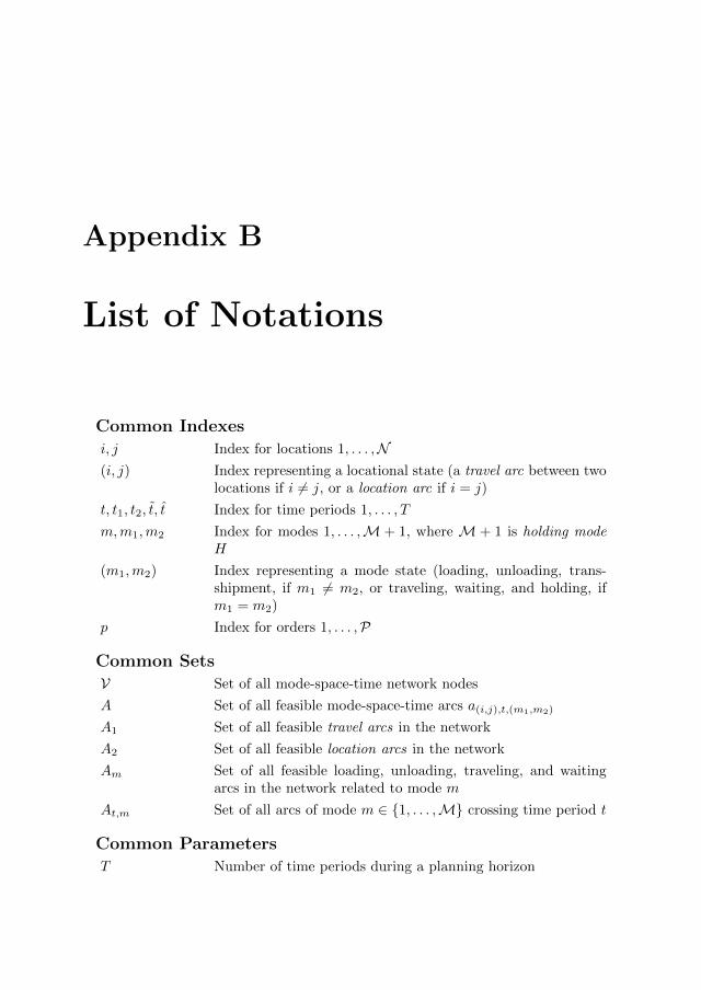
Appendix B
List of Notations
Common Indexesi, j Index for locations 1, . . . ,N(i, j) Index representing a locational state (a travel arc between two
locations if i 6= j, or a location arc if i = j)
t, t1, t2, t, t Index for time periods 1, . . . , T
m,m1,m2 Index for modes 1, . . . ,M + 1, where M + 1 is holding modeH
(m1,m2) Index representing a mode state (loading, unloading, trans-shipment, if m1 6= m2, or traveling, waiting, and holding, ifm1 = m2)
p Index for orders 1, . . . ,P
Common SetsV Set of all mode-space-time network nodes
A Set of all feasible mode-space-time arcs a(i,j),t,(m1,m2)
A1 Set of all feasible travel arcs in the network
A2 Set of all feasible location arcs in the network
Am Set of all feasible loading, unloading, traveling, and waitingarcs in the network related to mode m
At,m Set of all arcs of mode m ∈ {1, . . . ,M} crossing time period t
Common ParametersT Number of time periods during a planning horizon

160 Chapter B. List of Notations
P Number of orders
N Number of hub locations
M Number of transportation modes
speedm Speed of mode m
capm Capacity of mode m
Fm Maximum number of available vehicles for mode m
lm, lm(i,j),t Temperature of mode m for traveling between locations i andj starting at time t
utilm Average utilization percentage of mode m
VAT A coefficient used to show the higher cost of transporting ladenRTIs compared to empty ones
dist(i,j) Geographical distance between locations i and j
rm, rm(i,j),t Travel time of mode m for traveling between locations i and jstarting at time t
ri, r(m1,m2)i,t Operation time inside location i starting at time t
Cmfix Fixed (e.g. administration) cost of operating mode m
CmHR Cost of operating mode m per hour
CmKM Cost of operating mode m per Kilometer
Cm Cost of using one vehicle of mode m (Cm = Cmfix + CmKM ×dist(i,j))
Cmladen Variable cost of moving laden RTIs by mode m per time period(Cmladen = VAT× CmHR/(cap
m × utilm))
Cmempty Variable cost of repositioning empty RTIs by mode m per timeperiod (Cmempty = CmHR/(cap
m × utilm))
Choldi Cost of holding RTIs at location i (for single-RTI model)
C(m1,m2)i A general term for costs (loading, unloading, and holding) per
RTI per time period at location i
Si Number of available empty RTIs at location i (for single-RTImodel)
li, li,t Temperature inside location i at time t
wp Demand volume based on number of RTIs for order p
O(p) Origin location for order p
D(p) Destination location for order p
PT (p) The earliest time that order p is available for pickup at O(p)
DT (p) The latest delivery time for order p at D(p)
Lp Vaselife of order p (time× temperature)a(i,j),t,(m1,m2) A given (travel or location) arc in the mode-space-time network

161
Common Variablesxcatp,(i,j),t,(m1,m2) Nonnegative variable representing flow of RTIs of cat ∈
{laden, empty, repos} for order p, on location state (i, j)starting at time t, on mode state (m1,m2)
xladenp,(i,j),t,(m1,m2) Nonnegative variable representing flow of RTIs of cat ∈
{laden, empty, repos} for order p, on location state (i, j)finishing at time t, on mode state (m1,m2)
bp,(i,j),t,(m1,m2) Binary variable equal to 1, if flow of laden RTIs for order p istraversed on location state (i, j) starting at time t, on modestate (m1,m2), and 0, if not
U catpit Real variable representing the demand (supply, if negative) of
RTIs of cat ∈ {laden, empty, repos} for order p at location iat time point t
y(i,j),t,(m1,m2) Nonnegative variable representing the number of vehicles usedon location state (i, j) starting at time t, on mode state(m1,m2)
Additions for the ALNSz, z′ A solution
z0 Initial solution
z? Optimal solution
F(z) Objective (cost) function of solution z
FDes Total cost of the destroyed part of a solution
FRep Total cost of the repaired part of a solution
∆(Fe) Cost change of iteration e
q Index for order 1, . . . ,Q in a neighborhood
Q Number of orders in each ALNS neighborhood
Rp, Rq, Rcatp Route for order p or q (in cat ∈ {laden, empty, repos})
fm(i,j),t Fleet of mode m used to travel on (i, j) at time t
S Number of supply locations in the assignment problem
D Number of demand locations in the assignment problem
si Supply location i in the assignment problem
dj Demand location j in the assignment problem
xm(i,j),(t1,t2) Nonnegative variable representing the number of RTIs assignedfrom location i to location j with the pickup time t1 anddelivery deadline of t2, transported by mode m

162 Chapter B. List of Notations
rm(i,j),t1 Travel time of mode m between locations i and j starting attime t1
EDmij Earliest possible depart time of a mode m traveling between
locations i and j
LDmij Latest possible depart time of a mode m traveling between
locations i and j
β Difference in pickup times PT (p) and PT (q) (or their deliverytime DT (p) and DT (q)) of two orders p and q
DOpers Total number of destroy operators
ROpers Total number of repair operators
ωi,e Weight of operator i in iteration e
θ, θ1, θ2, θ3, θ4 Scores to evaluate the performance of operators
λ Reaction factor controlling the reaction of operators to thechanges in an iteration
∆(time)e Computation time of an iteration e
π Stopping criterion of ANS-1
η Stopping criterion of ANS-2
Additions for the Rolling Horizon Frameworkφ Index of a roll φ = 1, 2, 3, . . .
zφ Solution of roll φ
T Number of time periods during a planning horizon φ, φ +1, . . . , φ+ T in a roll φ
τ Length of a roll
α1, α2, α3 Weights for concentrating the improvement on orders of t =φ, φ+ 1, φ+ 2, . . .
ξ End-of-the-week required percentage of RTI storage level Si atlocation i
Additions for the Stochastic Two-Stage Programp′ Index for future orders 1, . . . ,P ′
wp′ Random daily demand volume based on number of RTIs fororder p′
Ψ(wp′)) Distribution function of daily demand volume for order p′
µp′ Daily average of demand volume for order p′
θp′ Ad-hoc capacity increase for order p′
Cθ Variable cost of outsourcing per unit of RTI
γ Index for scenario 1, . . . ,Γ
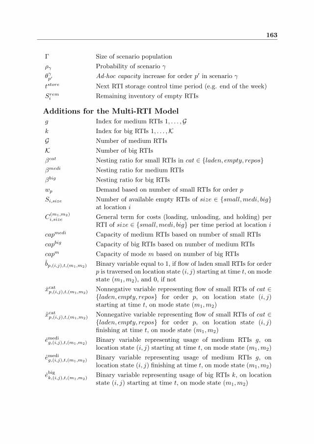
163
Γ Size of scenario population
ργ Probability of scenario γ
θγp′ Ad-hoc capacity increase for order p′ in scenario γ
tstore Next RTI storage control time period (e.g. end of the week)
Sremi Remaining inventory of empty RTIs
Additions for the Multi-RTI Modelg Index for medium RTIs 1, . . . ,Gk Index for big RTIs 1, . . . ,KG Number of medium RTIs
K Number of big RTIs
βcat Nesting ratio for small RTIs in cat ∈ {laden, empty, repos}βmedi Nesting ratio for medium RTIs
βbig Nesting ratio for big RTIs
wp Demand based on number of small RTIs for order p
Si,size Number of available empty RTIs of size ∈ {small,medi, big}at location i
C(m1,m2)i,size General term for costs (loading, unloading, and holding) per
RTI of size ∈ {small,medi, big} per time period at location i
capmedi Capacity of medium RTIs based on number of small RTIs
capbig Capacity of big RTIs based on number of medium RTIs
capm Capacity of mode m based on number of big RTIs
bp,(i,j),t,(m1,m2) Binary variable equal to 1, if flow of laden small RTIs for orderp is traversed on location state (i, j) starting at time t, on modestate (m1,m2), and 0, if not
xcatp,(i,j),t,(m1,m2) Nonnegative variable representing flow of small RTIs of cat ∈
{laden, empty, repos} for order p, on location state (i, j)starting at time t, on mode state (m1,m2)
xcatp,(i,j),t,(m1,m2) Nonnegative variable representing flow of small RTIs of cat ∈
{laden, empty, repos} for order p, on location state (i, j)finishing at time t, on mode state (m1,m2)
emedig,(i,j),t,(m1,m2) Binary variable representing usage of medium RTIs g, on
location state (i, j) starting at time t, on mode state (m1,m2)
emedig,(i,j),t,(m1,m2) Binary variable representing usage of medium RTIs g, on
location state (i, j) finishing at time t, on mode state (m1,m2)
ebigk,(i,j),t,(m1,m2) Binary variable representing usage of big RTIs k, on location
state (i, j) starting at time t, on mode state (m1,m2)
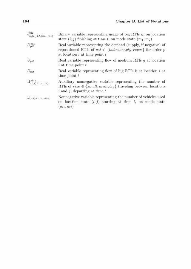
164 Chapter B. List of Notations
ebigk,(i,j),t,(m1,m2) Binary variable representing usage of big RTIs k, on location
state (i, j) finishing at time t, on mode state (m1,m2)
U catpit Real variable representing the demand (supply, if negative) of
repositioned RTIs of cat ∈ {laden, empty, repos} for order pat location i at time point t
Ugit Real variable representing flow of medium RTIs g at locationi at time point t
Ukit Real variable representing flow of big RTIs k at location i attime point t
Πsize(i,j),t,(m,m) Auxiliary nonnegative variable representing the number of
RTIs of size ∈ {small,medi, big} traveling between locationsi and j, departing at time t
y(i,j),t,(m1,m2) Nonnegative variable representing the number of vehicles usedon location state (i, j) starting at time t, on mode state(m1,m2)

Bibliography
R. Agarwal and O. Ergun. Ship scheduling and network design for cargo routing inliner shipping. Transportation Science, 42(2):175–196, 2008.
J. Ahmt, J.S. Sigtenbjerggaard, R.M. Lusby, J. Larsen, and D. Ryan. A new approachto the container positioning problem. Flexible Services and Manufacturing Journal,pages 1–27, 2015.
O. Ahumada and J.R. Villalobos. Application of planning models in the agri-foodsupply chain: A review. European journal of Operational research, 196(1):1–20,2009.
O. Ahumada and J.R. Villalobos. A tactical model for planning the production anddistribution of fresh produce. Annals of Operations Research, 190(1):339–358, 2011.
AI. ISO container price guide, 2016. URL http://www.approvedindex.co.uk/
storage-containers/iso-containers.
R. Akkerman, P. Farahani, and M. Grunow. Quality, safety and sustainability infood distribution: A review of quantitative operations management approachesand challenges. Or Spectrum, 32(4):863–904, 2010.
K. An and H.K. Lo. Ferry service network design with stochastic demand under userequilibrium flows. Transportation Research Part B: Methodological, 66:70–89, 2014.
J. Andersen and M. Christiansen. Designing new European rail freight services.Journal of the Operational Research Society, 60(3):348–360, 2009.
J. Andersen, T.G. Crainic, and M. Christiansen. Service network design withmanagement and coordination of multiple fleets. European Journal of OperationalResearch, 193(2):377–389, 2009a.
J. Andersen, T.G. Crainic, and M. Christiansen. Service network design with assetmanagement: Formulations and comparative analyses. Transportation ResearchPart C: Emerging Technologies, 17(2):197–207, 2009b.
J. Andersen, M. Christiansen, T.G. Crainic, and R. Grønhaug. Branch and price for

166 Bibliography
service network design with asset management constraints. Transportation Science,45(1):33–49, 2011.
D. Anghinolfi, M. Paolucci, S. Sacone, and S. Siri. Freight transportation in railwaynetworks with automated terminals: A mathematical model and MIP heuristicapproaches. European Journal of Operational Research, 214(3):588–594, 2011.
R.K. Apaiah and E.M.T. Hendrix. Design of a supply chain network for pea-basednovel protein foods. Journal of Food Engineering, 70(3):383–391, 2005.
A. Atamturk and M. Zhang. Two-stage robust network flow and design under demanduncertainty. Operations Research, 55(4):662–673, 2007.
B. Ayar and H. Yaman. An intermodal multicommodity routing problem withscheduled services. Computational Optimization and Applications, 53(1):131–153,2012.
R. Bai, G. Kendall, R. Qu, and J.A.D. Atkin. Tabu assisted guided local searchapproaches for freight service network design. Information Sciences, 189:266–281,2012.
R. Bai, S.W. Wallace, J. Li, and A.Y.L. Chong. Stochastic service network designwith rerouting. Transportation Research Part B: Methodological, 60:50–65, 2014.
A. Balakrishnan, T.L. Magnanti, and P. Mirchandani. Network design. InM. Dell’Amico, F. Maffoli, and S. Martello, editors, Annotated Bibliographies inCombinatorial Optimization, chapter 16, pages 311–334. 1997.
R. Baldacci, M. Battarra, and D. Vigo. Routing a heterogeneous fleet of vehicles.In B. Golden, S. Raghavan, and E. Wasil, editors, The Vehicle Routing Problem:Latest Advances and New Challenges, chapter 1, pages 3–27. 2010.
D.L. Bandeira, J.L. Becker, and D. Borenstein. A DSS for integrated distribution ofempty and full containers. Decision Support Systems, 47(4):383–397, 2009.
J. Bauer, T. Bektas, and T.G. Crainic. Minimizing greenhouse gas emissions inintermodal freight transport: An application to rail service design. Journal of theOperational Research Society, 61(3):530–542, 2010.
T. Bektas and T.G. Crainic. A brief overview of intermodal transportation. TechnicalReport 3, CIRRELT, 2007.
T. Bektas, M. Chouman, and T.G. Crainic. Lagrangean-based decompositionalgorithms for multicommodity network design problems with penalized constraints.Networks, 55(3):171–180, 2010.
S. Bock. Real-time control of freight forwarder transportation networks by integratingmultimodal transport chains. European Journal of Operational Research, 200(3):733–746, 2010.
Y.M. Bontekoning, C. Macharis, and J.J. Trip. Is a new applied transportation

Bibliography 167
research field emerging - a review of intermodal rail-truck freight transportliterature. Transportation Research Part A: Policy and Practice, 38(1):1–34, 2004.
M. Bortolini, M. Faccio, E. Ferrari, M. Gamberi, and F. Pilati. Fresh food sustainabledistribution: Cost, delivery time and carbon footprint three-objective optimization.Journal of Food Engineering, 174:56–67, 2016.
B. Bouzaiene-Ayari, C. Cheng, S. Das, R. Fiorillo, and W.B. Powell. From singlecommodity to multiattribute models for locomotive optimization: A comparisonof optimal integer programming and approximate dynamic programming.Transportation Science, 50(2):366–389, 2014.
K. Braekers, A. Caris, and G.K. Janssens. Optimal shipping routes and vessel sizefor intermodal barge transport with empty container repositioning. Computers inindustry, 64(2):155–164, 2013.
B.D. Brouer, J.F. Alvarez, C.E.M. Plum, D. Pisinger, and M.M. Sigurd. A baseinteger programming model and benchmark suite for liner-shipping network design.Transportation Science, 48(2):281–312, 2013.
B.D. Brouer, G. Desaulniers, and D. Pisinger. A matheuristic for the linershipping network design problem. Transportation Research Part E: Logistics andTransportation Review, 72:42–59, 2014.
V. Cacchiani, A. Caprara, L. Galli, L. Kroon, G. Maroti, and P. Toth. Railway rollingstock planning: Robustness against large disruptions. Transportation Science, 46(2):217–232, 2012.
D. Canca, A. De-Los-Santos, G. Laporte, and J.A. Mesa. An adaptive neighborhoodsearch metaheuristic for the integrated railway rapid transit network design andline planning problem. Computers & Operations Research, 78:1–14, 2017.
A. Caris, C. Macharis, and G.K. Janssens. Decision support in intermodal transport:A new research agenda. Computers in Industry, 64.
A. Caris, C. Macharis, and G.K. Janssens. Corridor network design in hinterlandtransportation systems. Flexible Services and Manufacturing Journal, 24(3):294–319, 2012.
CEC. Keep europe moving - Sustainable mobility for our continent, 2006. URL http:
//europa.eu/rapid/press-release_IP-06-818_en.htm?locale=en. ISBN: 92-79-02312-8.
H. Chang, H. Jula, A. Chassiakos, and P. Ioannou. A heuristic solution for theempty container substitution problem. Transportation Research Part E: Logisticsand Transportation Review, 44(2):203–216, 2008.
T.S. Chang. Best routes selection in international intermodal networks. Computers& operations research, 35(9):2877–2891, 2008.

168 Bibliography
H.K. Chen, C.F. Hsueh, and M.S. Chang. The real-time time-dependent vehiclerouting problem. Transportation Research Part E: Logistics and TransportationReview, 42(5):383–408, 2006.
L. Chen and E. Miller-Hooks. Resilience: An indicator of recovery capability inintermodal freight transport. Transportation Science, 46(1):109–123, 2012.
J.H. Cho, H.S. Kim, and H.R. Choi. An intermodal transport network planningalgorithm using dynamic programming – a case study: From Busan to Rotterdamin intermodal freight routing. Applied Intelligence, 36(3):529–541, 2012.
S.T. Choong, M.H. Cole, and E. Kutanoglu. Empty container management forintermodal transportation networks. Transportation Research Part E: Logisticsand Transportation Review, 38(6):423–438, 2002.
M. Chouman and T.G. Crainic. A MIP-tabu search hybrid framework formulticommodity capacitated fixed-charge network design. Technical Report 31,CIRRELT, 2010.
M. Chouman and T.G. Crainic. MIP-based tabu search for service network designwith design-balanced requirements. Technical Report 68, CIRRELT, 2011.
M. Chouman and T.G. Crainic. Cutting-plane matheuristic for service network designwith design-balanced requirements. Transportation Science, 49(1):99–113, 2014.
M. Chouman, T.G. Crainic, and B. Gendron. Commodity representations and cutset-based inequalities for multicommodity capacitated fixed-charge network design.Technical Report 56, CIRRELT, 2011.
CHP. How much does it cost to transport a shipping container?,2016. URL http://www.containerhomeplans.org/2015/07/
how-much-does-it-cost-to-transport-a-shipping-container/.
M. Christiansen, K. Fagerholt, B. Nygreen, and D. Ronen. Maritime transportation.In C. Barnhart and G. Laporte, editors, Transportation, volume 14 of Handbooksin Operations Research and Management Science, pages 189–284. 2007.
A. Cohn, M. Davey, L. Schkade, A. Siegel, and C. Wong. Network design and flowproblems with cross-arc costs. European Journal of Operational Research, 189(3):890–901, 2008.
J.F. Cordeau, M. Dell’Amico, S. Falavigna, and M. Iori. A rolling horizon algorithmfor auto-carrier transportation. Transportation Research Part B: Methodological,76:68–80, 2015.
A.M. Costa. A survey on Benders decomposition applied to fixed-charge networkdesign problems. Computers & operations research, 32(6):1429–1450, 2005.
A.M. Costa, J.F. Cordeau, and B. Gendron. Benders, metric and cutset inequalitiesfor multicommodity capacitated network design. Computational Optimization and

Bibliography 169
Applications, 42(3):371–392, 2009.
T. G. Crainic, M. Gendreau, and J. M. Farvolden. A simplex-based tabu searchmethod for capacitated network design. INFORMS Journal on Computing, 12(3):223–236, 2000.
T.G. Crainic. Long-haul freight transportation. In R.W. Hall, editor, Handbook ofTransportation Science, volume 56 of International Series in Operations Researchand Management Science, pages 451–516. 2003.
T.G. Crainic and K.H. Kim. Intermodal transportation. In C. Barnhart andG. Laporte, editors, Transportation, volume 14 of Handbooks in Operations Researchand Management Science, pages 467–537. 2007.
T.G. Crainic and G. Laporte. Planning models for freight transportation. Europeanjournal of operational research, 97(3):409–438, 1997.
T.G. Crainic, Y. Li, and M. Toulouse. A first multilevel cooperative algorithm forcapacitated multicommodity network design. Computers & Operations Research,33(9):2602–2622, 2006.
T.G. Crainic, M. Gendreau, and J.Y. Potvin. Intelligent freight-transportationsystems: Assessment and the contribution of operations research. TransportationResearch Part C: Emerging Technologies, 17(6):541–557, 2009.
T.G. Crainic, X. Fu, M. Gendreau, W. Rei, and S. Wallace. Progressive hedging-basedmetaheuristics for stochastic network design. Networks, 58(2):114–124, 2011.
T.G. Crainic, M. Hewitt, and W. Rei. Scenario grouping in a progressive hedging-based meta-heuristic for stochastic network design. Computers & OperationsResearch, 43:90–99, 2014.
T.G. Crainic, M. Hewitt, M. Toulouse, and D.M. Vu. Service network design withresource constraints. Transportation Science, 50(4):1380–1393, 2016.
K.L. Croxton, B. Gendron, and T.L. Magnanti. Variable disaggregation in networkflow problems with piecewise linear costs. Operations research, 55(1):146–157, 2007.
DAVINC3I. Dutch Agricultural Virtualized International Network with Coordination,Consolidation, Collaboration, and Information availablity project, 2011. URLhttp://www.davinc3i.com/.
E. Demir, W. Burgholzer, M. Hrusovsky, E. Arıkan, W. Jammernegg, and T. vanWoensel. A green intermodal service network design problem with travel timeuncertainty. Transportation Research Part B: Methodological, pages 1–19, 2015.
U. Derigs, J. Gottlieb, J. Kalkoff, M. Piesche, F. Rothlauf, and U. Vogel. Vehiclerouting with compartments: Applications, modelling and heuristics. OR spectrum,33(4):885–914, 2011.
M. Di Francesco, M. Lai, and P. Zuddas. Maritime repositioning of empty containers

170 Bibliography
under uncertain port disruptions. Computers & Industrial Engineering, 64(3):827–837, 2013.
K.F. Doerner, M. Gronalt, R.F. Hartl, G. Kiechle, and M. Reimann. Exact andheuristic algorithms for the vehicle routing problem with multiple interdependenttime windows. Computers & Operations Research, 35(9):3034–3048, 2008.
A.L. Erera, J.C. Morales, and M. Savelsbergh. Global intermodal tank containermanagement for the chemical industry. Transportation Research Part E: Logisticsand Transportation Review, 41(6):551–566, 2005.
EUROSTAT. EU transport in figures - Statistical pocketbook, 2012. URLhttp://ec.europa.eu/transport/facts-fundings/statistics/doc/2012/
pocketbook2012.pdf. ISBN: 978-92-79-21694-7.
EVO. Besparen in ketens – sierteeltsector, ketens in kaart brengen,2009. URL http://www.agrologistiek.nl/downloads/Eindrapportage%
20BiK-sierteelt%202-3-2009.pdf.
FloraHolland. Annual report, 2015. URL https://www.royalfloraholland.com/
en/about-floraholland/media-centre/annual-report-2015/.
J. Garcıa, J.E. Florez, A. Torralba, Da. Borrajo, C.L. Lopez, A. Garcıa-Olaya,and J. Saenz. Combining linear programming and automated planning to solveintermodal transportation problems. European Journal of Operational Research,227(1):216–226, 2013.
M. Garg and J.C. Smith. Models and algorithms for the design of survivablemulticommodity flow networks with general failure scenarios. Omega, 36(6):1057–1071, 2008.
S. Gelareh and D. Pisinger. Fleet deployment, network design and hub location of linershipping companies. Transportation Research Part E: Logistics and TransportationReview, 47(6):947–964, 2011.
M. Gendreau, F. Guertin, J.Y. Potvin, and R. Seguin. Neighborhood searchheuristics for a dynamic vehicle dispatching problem with pick-ups and deliveries.Transportation Research Part C: Emerging Technologies, 14(3):157–174, 2006.
M. Gendreau, G. Ghiani, and E. Guerriero. Time-dependent routing problems: Areview. Computers & Operations Research, 64:189–197, 2015.
B. Gendron and M. Larose. Branch-and-price-and-cut for large-scale multicommoditycapacitated fixed-charge network design. EURO Journal on ComputationalOptimization, 2(1–2):55–75, 2014.
I. Ghamlouche, T. G. Crainic, and M. Gendreau. Cycle-based neighbourhoods forfixed-charge capacitated multicommodity network design. Operations research, 51(4):655–667, 2003.

Bibliography 171
A.H. Gharehgozli, G. Laporte, Y. Yu, and R. de Koster. Scheduling twin yard cranesin a container block. Transportation Science, 49(3):686–705, 2014.
G. Ghiani, F. Guerriero, G. Laporte, and R. Musmanno. Real-time vehicle routing:Solution concepts, algorithms and parallel computing strategies. European Journalof Operational Research, 151(1):1–11, 2003.
G. Ghiani, G. Laporte, and R. Musmanno. Introduction to Logistics SystemsManagement. John Wiley and Sons, 2013.
J.K. Gigler, E.M.T. Hendrix, R.A. Heesen, V.G.W. Van Den Hazelkamp, andG. Meerdink. On optimisation of agri chains by dynamic programming. EuropeanJournal of Operational Research, 139(3):613–625, 2002.
A. Goel. The value of in-transit visibility for supply chains with multiple modes oftransport. International Journal of Logistics: Research and Applications, 13(6):475–492, 2010.
M.F. Gorman, J.P. Clarke, A.H. Gharehgozli, M. Hewitt, R. de Koster, and D. Roy.State of the practice: A review of the application of or/ms in freight transportation.Interfaces, 44(6):535–554, 2014.
P. Grangier, M. Gendreau, F. Lehuede, and L.M. Rousseau. An adaptive largeneighborhood search for the two-echelon multiple-trip vehicle routing problem withsatellite synchronization. European Journal of Operational Research, 254(1):80–91,2016.
S. Hamzaoui and O. Ben-Ayed. Parcel distribution timetabling problem. OperationsManagement Research, 4(3-4):138–149, 2011.
A. Hemmati, L.M. Hvattum, M. Christiansen, and G. Laporte. An iterative two-phase hybrid matheuristic for a multi-product short sea inventory-routing problem.European Journal of Operational Research, 252(3):775–788, 2016.
M. Hewitt, G. Nemhauser, and M.W.P. Savelsbergh. Combining exact and heuristicapproaches for the capacitated fixed-charge network flow problem. INFORMSJournal on Computing, 22(2):314–325, 2010.
M. Hewitt, G. Nemhauser, and M.W.P. Savelsbergh. Branch-and-price guided searchfor integer programs with an application to the multicommodity fixed-chargenetwork flow problem. INFORMS Journal on Computing, 25(2):302–316, 2013.
A. Hoff, A.G. Lium, A. Løkketangen, and T.G. Crainic. A metaheuristic for stochasticservice network design. Journal of Heuristics, 16(5):653–679, 2010.
L. Hong. An improved LNS algorithm for real-time vehicle routing problem with timewindows. Computers & Operations Research, 39(2):151–163, 2012.
C.I. Hsu and Y.P. Hsieh. Routing, ship size, and sailing frequency decision-makingfor a maritime hub-and-spoke container network. Mathematical and Computer

172 Bibliography
Modelling, 45(7):899–916, 2007.
C.I. Hsu, S.F. Hung, and H.C. Li. Vehicle routing problem with time-windows forperishable food delivery. Journal of food engineering, 80(2):465–475, 2007.
X. Hu, Z. Wang, M. Huang, and A.Z. Zeng. A computer-enabled solution procedurefor food wholesalers’ distribution decision in cities with a circular transportationinfrastructure. Computers & Operations Research, 36(7):2201–2209, 2009.
M. Huang, X. Hu, and L. Zhang. A decision method for disruption managementproblem in intermodal freight transport. In J. Watada, G. Phillips-Wren, L.C.Jain, and R.J. Howlett, editors, Intelligent Decision Technologies, volume 10 ofSmart Innovation, Systems and Technologies, pages 13–21. 2011.
ITC. International trade statistics 2001–2015, 2016. URL http://www.intracen.
org/itc/market-info-tools/trade-statistics/.
C.V. Karsten, B.D. Brouer, G. Desaulniers, and D. Pisinger. Time constrainedliner shipping network design. Transportation Research Part E: Logistics andTransportation Review, 2016. Article in press.
S.W. Lam, L.H. Lee, and L.C. Tang. An approximate dynamic programming approachfor the empty container allocation problem. Transportation Research Part C:Emerging Technologies, 15(4):265–277, 2007.
G. Laporte. Fifty years of vehicle routing. Transportation Science, 43(4):408–416,2009.
A. Larsen, O.B.G. Madsen, and M.M. Solomon. Recent developments in dynamicvehicle routing systems. In B. Golden, S. Raghavan, and E. Wasil, editors, TheVehicle Routing Problem: Latest Advances and New Challenges, pages 199–218.2008.
J.Q. Li, P.B. Mirchandani, and D. Borenstein. Real-time vehicle rerouting problemswith time windows. European Journal of Operational Research, 194(3):711–727,2009.
X. Li, K. Wei, Y.P. Aneja, and P. Tian. Design-balanced capacitated multicommoditynetwork design with heterogeneous assets. Omega, 2016. Article in press.
C.C. Lin and S.H. Chen. An integral constrained generalized hub-and-spoke networkdesign problem. Transportation Research Part E: Logistics and TransportationReview, 44(6):986–1003, 2008.
A.G. Lium, T.G. Crainic, and S.W. Wallace. A study of demand stochasticity inservice network design. Transportation Science, 43(2):144–157, 2009.
C. Macharis and Y.M. Bontekoning. Opportunities for or in intermodal freighttransport research - a review. European Journal of operational research, 153(2):400–416, 2004.

Bibliography 173
G.R. Mauri, G.M. Ribeiro, L.A.N Lorena, and G. Laporte. An adaptive largeneighborhood search for the discrete and continuous berth allocation problem.Computers & Operations Research, 70:140–154, 2016.
J.E. Mendoza, B. Castanier, C. Gueret, A.L. Madaglia, and N. Velasco. Constructiveheuristics for the multicompartment vehicle routing problem with stochasticdemands. Transportation Science, 45(3):346–363, 2011.
Q. Meng and S. Wang. Liner shipping service network design with empty containerrepositioning. Transportation Research Part E: Logistics and TransportationReview, 47(5):695–708, 2011.
Q. Meng, T. Wang, and S. Wang. Short-term liner ship fleet planning with containertransshipment and uncertain container shipment demand. European Journal ofOperational Research, 223(1):96–105, 2012.
E. Miller-Hooks, X. Zhang, and R. Faturechi. Measuring and maximizing resilienceof freight transportation networks. Computers & Operations Research, 39(7):1633–1643, 2012.
V.D. Minh, T.G. Crainic, and M. Toulouse. A three-stage matheuristic forthe capacitated multi-commodity fixed-cost network design with design-balanceconstraints. Technical Report 21, CIRRELT, 2012.
S. Mitrovic-Minic, R. Krishnamurti, and G. Laporte. Double-horizon based heuristicsfor the dynamic pickup and delivery problem with time windows. TransportationResearch Part B: Methodological, 38(8):669–685, 2004.
L. Moccia, J.F. Cordeau, G. Laporte, S. Ropke, and M.P. Valentini. Modelingand solving a multimodal transportation problem with flexible time and scheduledservices. Networks, 57(1):53–68, 2011.
L.K. Nielsen, L. Kroonb, and G. Maroti. A rolling horizon approach for disruptionmanagement of railway rolling stock. European Journal of Operational Research,220(2):496–509, 2012.
A. Osvald and L.Z. Stirn. A vehicle routing algorithm for the distribution of freshvegetables and similar perishable food. Journal of food engineering, 85(2):285–295,2008.
D.C. Paraskevopoulos, T. Bektas, Crainic. T.G., and C.N. Potts. A cycle-basedevolutionary algorithm for the fixed-charge capacitated multi-commodity networkdesign problem. European Journal of Operational Research, 253(2):265–279, 2016a.
D.C. Paraskevopoulos, S. Gurel, and T. Bektas. The congested multicommoditynetwork design problem. Transportation Research Part E: Logistics andTransportation Review, 85:166–187, 2016b.
D. Parmenter. Key Performance Indicators: Developing, Implementing,and UsingWinning KPIs. John Wiley and Sons, 2007.

174 Bibliography
J.A. Pazour, R.D. Meller, and L.M. Pohl. A model to design a national high-speedrail network for freight distribution. Transportation Research Part A: Policy andPractice, 44(3):119–135, 2010.
M.B. Pedersen, T.G. Crainic, and O.B.G. Madsen. Models and tabu searchmetaheuristics for service network design with asset-balance requirements.Transportation Science, 43(2):158–177, 2009.
V. Pillac, M. Gendreau, C. Gueret, and A.L. Medaglia. A review of dynamic vehiclerouting problems. European Journal of Operational Research, 225(1):1–11, 2013.
D. Pisinger and S. Ropke. A general heuristic for vehicle routing problems. Computers& operations research, 34(8):2403–2435, 2007.
W.B. Powell. Dynamic models of transportation operations. In A.G. de Kok and S.C.Graves, editors, Supply Chain Management: Design, Coordination and Operation,volume 11 of Handbooks in Operations Research and Management Science, pages677–756. 2003.
W.B. Powell. Approximate dynamic programming: Lessons from the field. In S.J.Mason, R.R. Hill, L. Moench, and O. Rose, editors, Proceedings of the 2008 WinterSimulation Conference, pages 205–214, 2008.
W.B. Powell. What you should know about approximate dynamic programming.Naval Research Logistics, 56(3):239–249, 2009.
W.B. Powell, P. Jaillet, and A. Odoni. Stochastic and dynamic networks and routing.In M.O. Ball, T.L. Magnanti, C.L. Monma, and G.L. Nemhauser, editors, NetworkRouting, volume 8 of Handbooks in Operations Research and Management Science,pages 141–295. 1995.
W.B. Powell, H.O. Simao, and B. Bouzaiene-Ayari. Approximate dynamicprogramming in transportation and logistics: A unified framework. EURO Journalon Transportation and Logistics, 1(3):237–284, 2012.
C. Puettmann and H. Stadtler. A collaborative planning approach for intermodalfreight transportation. OR spectrum, 32(3):809–830, 2010.
J.G. Rakke, M. Stalhane, C.R. Moe, M. Christiansen, H. Andersson, K. Fagerholt,and I. Norstad. A rolling horizon heuristic for creating a liquefied natural gas annualdelivery program. Transportation Research Part C: Emerging Technologies, 19(5):896–911, 2011.
S.A. Reis and J.E. Leal. A deterministic mathematical model to support temporaland spatial decisions of the soybean supply chain. Journal of Transport Geography,43:48–58, 2015.
A.P. Rifai, H.T. Nguyen, and S.Z.M. Dawal. Multi-objective adaptive largeneighborhood search for distributed reentrant permutation flow shop scheduling.Applied Soft Computing, 40:42–57, 2016.

Bibliography 175
I. Rodrıguez-Martın and J.J. Salazar-Gonzalez. A local branching heuristic forthe capacitated fixed-charge network design problem. Computers & OperationsResearch, 37(3):575–581, 2010.
S. Ropke and D. Pisinger. An adaptive large neighborhood search heuristic for thepickup and delivery problem with time windows. Transportation science, 40(4):455–472, 2006.
A. Rosenboom. Development of a decision support system for an orchestrator in thehorticultural sector, 2014. Master Thesis, TUe School of Industrial Engineering.
A. Rubin. Frequency distributions. In Statistics for Evidence-based Practice andEvaluation, chapter 4, pages 33–47. 2010.
A. Rushton, P. Croucher, and P. Baker. Integrated logistics and the supply chain.In The Handbook of Logistics and Distribution Management: Understanding theSupply Chain, chapter 2, pages 16–31. 2014.
J. Schonberger. Adaptive demand peak management in online transport processplanning. OR spectrum, 32(3):831–859, 2010.
S. Sethi and G. Sorger. A theory of rolling horizon decision making. Annals ofOperations Research, 29(1):387–415, 1991.
N. Shi, H. Song, and W.B. Powell. The dynamic fleet management problem withuncertain demand and customer chosen service level. International Journal ofProduction Economics, 148:110–121, 2014.
K. Shintani, A. Imai, E. Nishimura, and Papadimitriou S. The container shippingnetwork design problem with empty container repositioning. TransportationResearch Part E: Logistics and Transportation Review, 43(1):39–59, 2007.
J. Shu and M. Song. Dynamic container deployment: Two-stage robust model,complexity, and computational results. INFORMS Journal on Computing, 26(1):135–149, 2013.
M. Sloof and B.V. Everest. Problem decomposition. In L.M.M. Tijskens, M.L.A.T.M.Hertog, and B.M. Nicolai, editors, Food Process Modeling, chapter 2, pages 19–34.2001.
D.P. Song and J.X. Dong. Cargo routing and empty container repositioning in multipleshipping service routes. Transportation Research Part B: Methodological, 46(10):1556–1575, 2012.
R. Stahlbock and S. Voß. Operations research at container terminals: A literatureupdate. OR spectrum, 30(1):1–52, 2008.
M. SteadieSeifi, N.P. Dellaert, W. Nuijten, T. van Woensel, and R. Raoufi.Multimodal freight transportation planning: A literature review. European journalof operational research, 233(1):1–15, 2014.

176 Bibliography
E.G. Talbi. Single-solution based metaheuristics. In Metaheuristics: From design toimplementions, chapter 2, pages 87–188. John Wiley and Sons, 2009.
P.S. Taoukis. Modeling the use of time-temperature indications in distribution andstock rotations. In L.M.M. Tijskens, M.L.A.T.M. Hertog, and B.M. Nicolai, editors,Food Process Modeling, chapter 19, pages 19–34. 2001.
C.D. Tarantilis and C.T. Kiranoudis. A meta-heuristic algorithm for the efficientdistribution of perishable food. Journal of food Engineering, 50(1):1–9, 2001.
C.D. Tarantilis and C.T. Kiranoudis. Distribution of fresh meat. Journal of FoodEngineering, 51(1):85–91, 2002.
N. Teypaz, S. Schrenk, and V.D. Cung. A decomposition scheme for large-scale servicenetwork design with asset management. Transportation Research Part E: Logisticsand Transportation Review, 46(1):156–170, 2010.
B. Thiongane, J.F. Cordeau, and B. Gendron. Formulations for the nonbifurcatedhop-constrained multicommodity capacitated fixed-charge network design problem.Computers & Operations Research, 53:1–8, 2015.
H. Topaloglu. A parallelizable dynamic fleet management model with random traveltimes. European Journal of Operational Research, 175(2):782–805, 2006.
H. Topaloglu. A parallelizable and approximate dynamic programming-based dynamicfleet management model with random travel times and multiple vehicle types.In V. Zeimpekis, C.D. Tarantilis, G.M. Giaglis, and I. Minis, editors, DynamicFleet Management, volume 38 of Operations Research/Computer Science InterfacesSeries. 2007.
H. Topaloglu and W.B. Powell. A distributed decision-making structure for dynamicresource allocation using nonlinear functional approximations. Operations Research,53(2):281–297, 2005.
H. Topaloglu and W.B. Powell. Dynamic-programming approximations for stochastictime-staged integer multicommodity-flow problems. INFORMS Journal onComputing, 18(1):31–42, 2006.
H. Topaloglu and W.B. Powell. Sensitivity analysis of a dynamic fleet managementmodel using approximate dynamic programming. Operations research, 55(2):319–331, 2007.
M. Tosi. Allocation of VALS activities in a metro model network in the Europeanfloricultural market, 2014. Master Thesis, Wageningen Department of SocialSciences.
UNECE. Illustrated glossary for transport statistics, 2009. URL http:
//epp.eurostat.ec.europa.eu/cache/ITY_OFFPUB/KS-RA-10-028/EN/
KS-RA-10-028-EN.PDF. ISBN: 978-92-79-17082-9.

Bibliography 177
W.J.A. van Heeswijk, M.R.K. Mes, J.M.J. Schutten, and W.H.M. Zijm. Freightconsolidation in intermodal networks with reloads. Flexible Services andManufacturing Journal, 2016. DOI 10.1007/s10696-016-9259-1.
Y. Van Hui, J. Gao, L. Leung, and S. Wallace. Airfreight forwarder’s shipmentplanning under uncertainty: A two-stage stochastic programming approach.Transportation Research Part E: Logistics and Transportation Review, 66:83–102,2014.
B. van Riessen, R.R. Negenborn, and R. Dekker. Synchromodal containertransportation: An overview of current topics and research opportunities. InInternational Conference on Computational Logistics, pages 386–397, 2015.
S. Verhoeven. Hub location decisions in the metromodel, 2014. Master Thesis, TUeSchool of Industrial Engineering.
M. Verma and V. Verter. A lead-time based approach for planning rail-truckintermodal transportation of dangerous goods. European Journal of OperationalResearch, 202(3):696–706, 2010.
M. Verma, V. Verter, and N. Zufferey. A bi-objective model for planning and managingrail-truck intermodal transportation of hazardous materials. Transportationresearch part E: logistics and transportation review, 48(1):132–149, 2012.
K. Verweij. Synchronic modalities - Critical success factors. In van der Sterre P.J.,editor, Logistics Yearbook edition 2011, pages 75–88. Rotterdam, 2011.
T. Vlassak. Future-proof return logistics in the floriculture sector, 2014. MasterThesis, TUe School of Industrial Engineering.
N. Wieberneit. Service network design for freight transportation: A review. ORspectrum, 30(1):77–112, 2008.
M. Yaghini, M. Karimi, M. Rahbar, and M.H. Sharifitabar. A cutting-planeneighborhood structure for fixed-charge capacitated multicommodity networkdesign problem. INFORMS Journal on Computing, 27(1):48–58, 2014.
J. Yang, P. Jaillet, and H. Mahmassani. Real-time multivehicle truckload pickup anddelivery problems. Transportation Science, 38(2):135–148, 2004.
E. Zhu, T.G. Crainic, and M. Gendreau. Scheduled service network design for freightrail transportation. Operations research, 62(2):383–400, 2014.
R.A. Zuidwijk and A.W. Veenstra. The value of information in container transport.Transportation Science, 49(3):675–685, 2014.


Summary
Multimodal Transportation for Perishable Products
Every day, a significant amount of perishable products are transported aroundEurope, each with their own characteristics and preservation requirements. Perishableproducts are products losing their value or quality over time, if not appropriatelystored or transported. Given short shelf-life of these products and high degree ofsupply and demand uncertainty, most industries resort to fast and direct transport(such as air or road) which are usually expensive, and not environmentally desirable.On the other hand, resorting to the cheapest transportation options, results in longerdelivery, and therefore, perished products. The focus of this thesis is on developingrelevant models and algorithms to find the trade-off between operational considerationand product quality preservation requirements.
A cheap and environmentally friendly long-haul transportation requires consolidationand switching from air and road to other modes of transport. Consolidation and modeswitching are the highlighted advantages of multimodal transportation. Multimodalfreight transportation is defined as the transportation of goods by a sequence ofat least two different modes of transportation. It offers a potential platform fora more efficient, reliable, flexible, and sustainable freight transportation. However,planning operations of a multimodal system added to the extra quality preservationof perishable products is heavily complex. Therefore, the main research questionin this thesis involves an improved understanding whether multimodal transportationplatform can be used for perishable products.
Despite gaining more attention, the literature on long-haul transportation of per-ishable products, especially with including temperature conditions in modelingproduct quality preservation measure, is very limited. Moreover, the key operationalchallenge of managing transportation resources, and more specifically, repositioningof the empty loading units called Returnable Transport Items (RTIs), deserves moreattention. RTIs can have different sizes ranging from a small box to a large 45-feetcontainer. Their number in the entire chain is limited, and their shortage at locationsthat they are needed results in quality decay of the products waiting for them, which
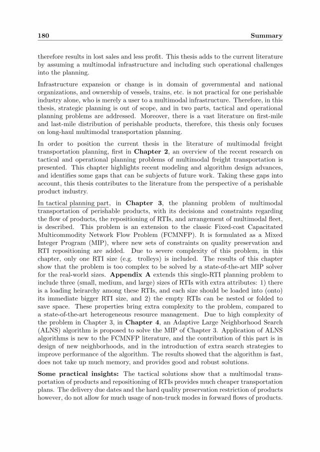
180 Summary
therefore results in lost sales and less profit. This thesis adds to the current literatureby assuming a multimodal infrastructure and including such operational challengesinto the planning.
Infrastructure expansion or change is in domain of governmental and nationalorganizations, and ownership of vessels, trains, etc. is not practical for one perishableindustry alone, who is merely a user to a multimodal infrastructure. Therefore, in thisthesis, strategic planning is out of scope, and in two parts, tactical and operationalplanning problems are addressed. Moreover, there is a vast literature on first-mileand last-mile distribution of perishable products, therefore, this thesis only focuseson long-haul multimodal transportation planning.
In order to position the current thesis in the literature of multimodal freighttransportation planning, first in Chapter 2, an overview of the recent research ontactical and operational planning problems of multimodal freight transportation ispresented. This chapter highlights recent modeling and algorithm design advances,and identifies some gaps that can be subjects of future work. Taking these gaps intoaccount, this thesis contributes to the literature from the perspective of a perishableproduct industry.
In tactical planning part, in Chapter 3, the planning problem of multimodaltransportation of perishable products, with its decisions and constraints regardingthe flow of products, the repositioning of RTIs, and arrangement of multimodal fleet,is described. This problem is an extension to the classic Fixed-cost CapacitatedMulticommodity Network Flow Problem (FCMNFP). It is formulated as a MixedInteger Program (MIP), where new sets of constraints on quality preservation andRTI repositioning are added. Due to severe complexity of this problem, in thischapter, only one RTI size (e.g. trolleys) is included. The results of this chaptershow that the problem is too complex to be solved by a state-of-the-art MIP solverfor the real-world sizes. Appendix A extends this single-RTI planning problem toinclude three (small, medium, and large) sizes of RTIs with extra attributes: 1) thereis a loading heirarchy among these RTIs, and each size should be loaded into (onto)its immediate bigger RTI size, and 2) the empty RTIs can be nested or folded tosave space. These properties bring extra complexity to the problem, compared toa state-of-the-art heterogeneous resource management. Due to high complexity ofthe problem in Chapter 3, in Chapter 4, an Adaptive Large Neighborhood Search(ALNS) algorithm is proposed to solve the MIP of Chapter 3. Application of ALNSalgorithms is new to the FCMNFP literature, and the contribution of this part is indesign of new neighborhoods, and in the introduction of extra search strategies toimprove performance of the algorithm. The results showed that the algorithm is fast,does not take up much memory, and provides good and robust solutions.
Some practical insights: The tactical solutions show that a multimodal trans-portation of products and repositioning of RTIs provides much cheaper transportationplans. The delivery due dates and the hard quality preservation restriction of productshowever, do not allow for much usage of non-truck modes in forward flows of products.

181
Trains and barges are mostly used for repositioning empty RTIs. Moreover, timelyrepositioning of empty RTIs is essential and no RTI of any type and size is anexception. Results show that having a central storage for all of them, close to thehubs with highest product flow traffic results in significant repositioning savings.
In operational planning part, Chapter 5 first describes the operational planningproblem of long-haul transportation of perishable products, with its decisions andconstraints. This problem is a dynamic extension to the planning problem of Chapter3, where at specific decision occasions (e.g. every 12 hours) and based on collecteddata on arrived demand and system evolution, a deterministic FCMNFP withupdated parameters on new demand, RTI repositioning, and available multimodaltransportation options, is reformulated and solved. Chapter 5 then presents a rolling-horizon framework to contain and control this decision process, where a modifiedversion of the ALNS of Chapter 4 is employed to provide new and adjusted plans, inorder to efficiently respond to the new demand and system changes. The solutionsof Chapter 5 however, rely only on revealed data, and do not include anticipationof future demand. Demand of perishable products fluctuates day to day, and thereare daily, weekly, and seasonal trends influencing the volume that each customerwants to transport. As a result, the solutions of Chapter 5 might end up eitheremploying last-minute expensive transportation options when demand is too high,or having underutilized fleet when demand is too low. In Chapter 6, demand isassumed to be stochastic, and the operational planning problem of Chapter 5 withstochastic demand is transformed into a dynamic and stochastic planning problem,where at each decision occasion, a Scenario-based Two-stage Stochastic Program(STSP) is reformulated and solved. This STSP is an extension to the planningproblem of Chapter 3, where at the first stage, the multimodal fleet is arrangedand at the second stage, this arrangement is used to find optimal product flow andRTI repositioning over a generated population of demand scenarios. The rolling-horizon framework of Chapter 5 is further extended to include these scenarios, andthe ALNS of Chapter 5 is also modified to include redesigned neighborhoods andparameter tuning. Therefore, at specific decision occasions, and after collectingarrived demand data, a scenario population for demand of the coming time periods isgenerated, and then by solving the STSP, new plans and adjustments are made. Withsimulating the results of both deterministic and stochastic planning frameworks, theinfluence of future demand anticipation is later analyzed. The application of rolling-horizon approaches in planning long-haul transportation operations is very limited,and Chapters 5 and 6 add to the literature by adapting it to the scope of this thesis,incorporating stochastic demand, and presenting vast analysis on its properties.
Some practical insights: The operational solutions show that in designing a goodoperational planning framework, a trade-off between cost and loss of sale should beconsidered. The shorter decision intervals are (e.g. every six hours), the less saleis lost. However, shorter intervals come with the price of having less informationabout the future. With less information, the chances of consolidation decrease, andthe arranged fleet is under-utilized. This problem is solved by incorporating an

182 Summary
anticipation of the future. In this thesis, uncertainty of future demand was takeninto account. This anticipation was obtained by analyzing historical data and trends,and generating scenarios representing their future possibilities. The results show thatincluding future demand uncertainty into the operational planning offers smarter andmore efficient fleet arrangement. Such plans provide a flexibility to tackle futuredemand fluctuations. There is however a trade-off between how many scenarios aregenerated and how much time is allowed for planning computations. It is desirable togenerate as many scenarios as possible, but the computational limits might not allowfinding good plans.
At the end of this thesis, Chapter 7 provides a summary of the findings, conclusions,practical insights, as well as the limitations of this thesis and future researchsuggestions. One of the limitations of this thesis is that the products are assumedhomogeneous, while in practice, perishable industries might share and combine theirlogistics to benefit from economy of scale. In such a setting, each product hasits own quality preservation requirement, and its preservation regime might not becompatible with others. Moreover, the objectives of the cooperating industries mightnot be congruent. Hence, extra constraints and multiple objectives are needed for thecombined long-haul transportation planning. This problem becomes more complex,and therefore, it might need different tactical and operational planning algorithms.Another future research suggestion is in the area of multi-size RTI management. Thisproblem is relatively new to the literature of multimodal transportation planning,and the loading and nesting relations among different sizes of RTIs make it extremelychallenging to model and to design efficient planning algorithms.
About the Author
Maryam SteadieSeifi was born on September 1st, 1982, in Tehran, Iran. She finishedher BSc in Industrial Engineering in 2004 at Alzahra University, and got her MSc inIndustrial Engineering in 2010 from Amirkabir University of Technology in Tehran.In the meantime, she worked for a few companies and a research institute, and thefocus of her studies and work was mainly in the area of logistics and transportationplanning.
In 2011, she started her PhD at Eindhoven University of Technology under thesupervision of Tom van Woensel and Nico Dellaert. During her PhD, together withWim Nuijten, Rasa Raoufi, and her supervisors, she published an award winningreview paper on multimodal freight transportation planning. The results of this PhDstudy, which Maryam defends on March 21st, 2017, are presented in this dissertation.