multidiscplinary control experiments based on the

“Proceedings of the 2001 American Society for Engineering Education Annual Conference & ExpositionCopyright 2001, American Society for Engineering Education”

Session 1526

MULTIDISCPLINARY CONTROL EXPERIMENTS BASED ON THEPROPORTIONAL-INTEGRAL-DERIVATIVE (PID) CONCEPT

Ravi P. Ramachandran, Raul Ordonez, Stephanie Farrell, Zenaida Otero Gephardt andHong Zhang

Faculty of Engineering, Rowan University, Glassboro, New Jersey 08028

Abstract - The hallmark of the newly configured Rowan College of Engineering undergraduate

program is multidisciplinary education with a laboratory emphasis. The development of a new

multidisciplinary control laboratory upholds our hallmark very well. We attempt to address the

demand of industry for acquiring control engineers (1) with a broad set of skills and a

comprehension of the diverse practical applications of control and (2) who can move across

rather artificial program boundaries with great ease. Multidisciplinary experiments that integrate

hands-on experience and software simulation are investigated. The experiments expose the

students to Proportional, Integral and Derivative (PID) control using a DC motor, engine speed

control apparatus and feedback process control. This enables electrical, mechanical and chemical

engineering students to learn the fundamental theory and physical implementation of various

types of control systems.

Introduction

The control systems laboratory is an integrated effort by the Faculty of Engineering at Rowan

University to configure a novel hands-on method of teaching Control Systems from a

multidisciplinary point of view. The Electrical, Mechanical and Chemical Engineering programs

are joining together to achieve this. Although Control is an interdisciplinary technology, there has

historically been a tendency for the different engineering departments to teach the subject from

their very own somewhat narrow perspective without any semblance of collaboration. This

project attempts to address the demand of industry for acquiring control engineers with a broad

set of skills and a comprehension of the diverse practical applications of Control [1]. This project

is in accordance with the multidisciplinary aim of our new programs and strives to meet the

requirements of industry in hiring control engineers who can move across rather artificial

program boundaries with great ease.


Goals and Objectives

Our aim is to accomplish the following:

1. Give students an exposure to the different aspects of control theory in the form of

multidisciplinary laboratory experiences that include electrical, mechanical, and process

control systems.

2. Ensure that our laboratory has an impact on a wide variety of courses in our curriculum.

3. Since digital technology is predominant in today’s industry, students should be exposed

to data acquisition and digital control for multidisciplinary purposes.

4. Integrate software simulation with hands-on laboratory work using MATLAB, its

associated SIMULINK package and C++ programming.

5. Expand student teamwork experience by having them work in groups on the laboratory

experiments.

6. Continue to improve written and oral communication skills of our students.

Description of Curriculum

Control education must integrate theory, hands-on experience and software simulation in a well

balanced fashion [1-8]. The laboratory will have a major impact on the control courses offered by

the Electrical, Mechanical and Chemical engineering departments and on other courses in the

curriculum that include the Engineering clinic, Fluid Mechanics, Mathematics for Engineering

Analysis, Digital Signal Processing and Digital Systems and Microprocessors. Our programs

include an interdisciplinary engineering clinic [9-12] every semester. Sharing many features in

common with the model for medical training, the clinic provides an atmosphere of faculty

mentoring in a hands-on, laboratory setting.

The control courses generally have three hours of laboratory per week in addition to two

to three hours of lectures. The curriculum in the control courses offered by the departments

include:

1. Basic system concepts: linearity, time-invariance, stability, frequency response, causality,

realizability, impulse response and transfer function (poles and zeros).

2. Mathematical modeling of physical systems: analogs between electrical, mechanical, fluid

and thermal systems and their circuit equivalence; differential equation description of


such systems and their analysis; Laplace transforms; block diagram algebra; signal flow

graphs.

3. Feedback: open loop and closed loop systems; pole placement; compensator design;

sensitivity analysis; steady-state error; performance criteria; proportional-integral-

derivative (PID) controllers.

4. Stability Analysis: Routh-Hurwitz criterion; root locus method; Nyquist criterion.

5. Frequency response analysis: Bode plots; gain and phase margins.

The basic differences in the lecture content of the courses lies in the emphasis on certain topics

and applications by the different departments. Electrical engineering students may see more

examples on circuits in the classroom while chemical engineers will see more examples on

process control. In the laboratory (common to all students), students will be exposed to a broad

range of applications of control theory. It is the experiments on PID control which are

summarized below.

Proportional-integral-derivative (PID) controllers

Figure 1: A general block diagram of a control system

A general block diagram of a control system is shown in Figure 1. All signals and system

functions are labeled as a function of the Laplace transform variable s [2]. The input and output

signals are denoted by X(s) and Y(s) respectively. The plant is denoted by G(s). The controller is

denoted by K(s) and the feedback loop has a system function H(s). The transfer function of the

system is given by T(s) = (K(s) G(s)) / ( 1 + K(s) G(s) H(s) ).

A PID controller has a system function K(s) = (K1 + K2s + K3/s) where K1 is the proportional

gain, K2 is the derivative gain and K3 is the integral gain. The popularity of PID controllers is due


to their functional simplicity of implementation (can be realized using simple active circuits) and

their robust performance in a wide range of operating conditions [2]. It is the control designer’s

task to determine the gains K1, K2 and K3 to satisfy certain performance criteria (like percent

overshoot, settling time and steady-state error) and maintain stability of the overall system. The

experiments described below are instructive in PID control and expose the students to a variety

of control systems.

Experiment 1: Engine Speed Control

The CE107 Engine Speed Control Apparatus demonstrates the problems encountered in

regulating the speed of rotating machines under varying load conditions, in particular, problems

with non-linear control systems. Some typical examples of such systems are:

1. An electrical generator being driven by a prime mover. In the case of the generator, a prime

mover such as an internal combustion engine or turbine, provide the input energy to be

converted into the output electrical energy. To maintain certain output voltage or frequency

levels from the generator under varying power loads, the prime mover speed must be kept

within the specified limits. This is accomplished by varying the fuel to the prime mover as

operating conditions change.

2. The 'Cruise Control' on a motor vehicle. This device allows the user to select a desired speed

at the beginning of a long journey. A feedback control system overrides the manual

accelerator setting to maintain the vehicle’s speed, irrespective of whether the road is level or

inclined or declined.

The apparatus is designed for control and analysis using an external control element. The

primary objective of the apparatus is to regulate the engine speed by manipulating the position of

the motorized valve under varying load conditions. All power supplies to drive the system and

sensor signal conditioning circuits are fully buffered and contained within the base of the CE107.

The circuits are accessed via the 2mm sockets mounted on the front panel.

The CE107 is composed of three individual systems, which are:

a. The Engine, Flywheel and Load Assemblyb. The Air Supplyc. The Motorized Valve


Figure 2: Front Panel of CE107 Engine Speed Control Apparatus

Air Supply Valve: Modeling

We will begin by examining the valve that is used to supply air to the system. The valve input

operates an electric motor, which turns at a rate proportional to the input voltage. The equation

modeling the dynamics of the system is given by:

ugdtdx

1=

where x is the valve position, u is the input voltage, and g1 is the drive valve motor gain.

This system works by having the valve position adjust the tension F on a control spring,

which in turn acts upon a diaphragm in the valve. If the tension is increased, then additional air

flows through an inlet and through the main valve. This allows the outlet pressure on the valve

to increase. The outlet pressure Po, exerts an opposite force on the diaphragm which acts against

the input tension. When the control spring tension and outlet are in equilibrium the airflow

through the valve stabilizes.

Engine and Load: Modeling

The air from the valve applies a pressure Po to the engine piston. This applied force is

transformed into an engine torque τe at the engine crankshaft. This means that the engine torque

τe is proportional to the pressure supplied by the valve


oee Pg=τ

where ge is the gain of the engine and crank assembly.

The engine torque is used to supply engine load, friction losses and to accelerate the

engine flywheel inertia I. Identifying the engine speed ω we can write the following equation:

��

�−��

��

�−��

��

�=��

��

�

TorqueFrictional

TorqueLoad

TorqueEngine

MomentumFlywheelofchangeofRate

____

or fledtdI τττω −−= . τf is proportional to the engine speed, that is, τf = bω.. Also, τl is

proportional to the load demand voltage dl, so that τl = gldl.

Valve Position and Speed Sensor Characteristics

There are two output variables; the valve position x and engine speed ω are measured by speed

sensing circuits. The valve position sensor is a potentiometer, which gives a voltage yx

proportional to the actual valve position,

xky vx ⋅=

An opto-electric sensor and the perforations on the flywheel sense the engine speed. The pulses

from the sensor are converted into a voltage yω, which is proportional to the engine speed.

ωω ⋅= sky

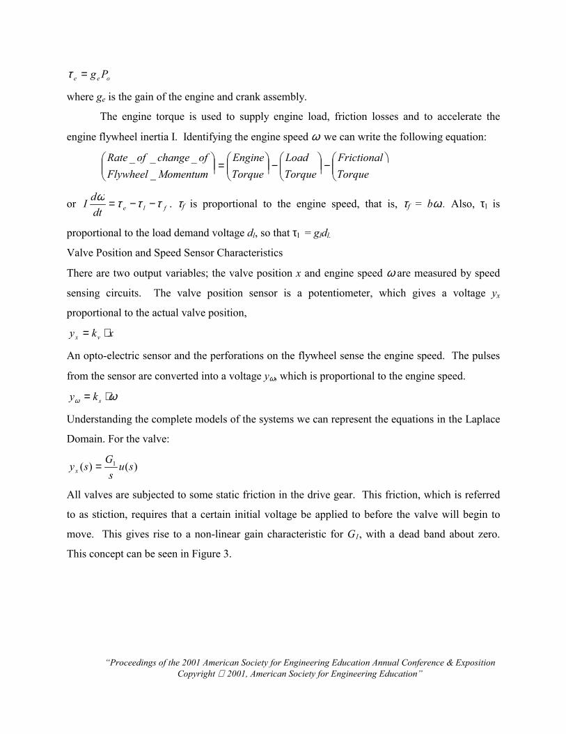
Understanding the complete models of the systems we can represent the equations in the Laplace

Domain. For the valve:

)()( 1 sus

Gsyx =

All valves are subjected to some static friction in the drive gear. This friction, which is referred

to as stiction, requires that a certain initial voltage be applied to before the valve will begin to

move. This gives rise to a non-linear gain characteristic for G1, with a dead band about zero.

This concept can be seen in Figure 3.


Figure 3: Non-Linear Gain Characteristic (Dead Band)

For the engine, we have

)(1

)(1

)( 2 sdsT

GsysT

Gsy ll

x +−

+=ω

The constant G2 is the gain of the system, which is the output voltage over the input voltage.

Here the input voltage will be the absolute value of the peak voltage of the step input, while the

output voltage will be the absolute value of the peak voltage measured at the terminal (ω) of the

motor. The value T is the pole of the system, which is obtained by analyzing the output voltage

waveform from the step input.

CE107 Block Diagram Development

It was observed that there was a non-linear effect associated with the gain of the air valve motor.

To reduce the effects of the non-linear gain, we will implement the method of local feedback.

The following figure illustrates the feedback loop with a gain k1 that is used to make the actual

valve position yx correspond to the desired valve position yr.


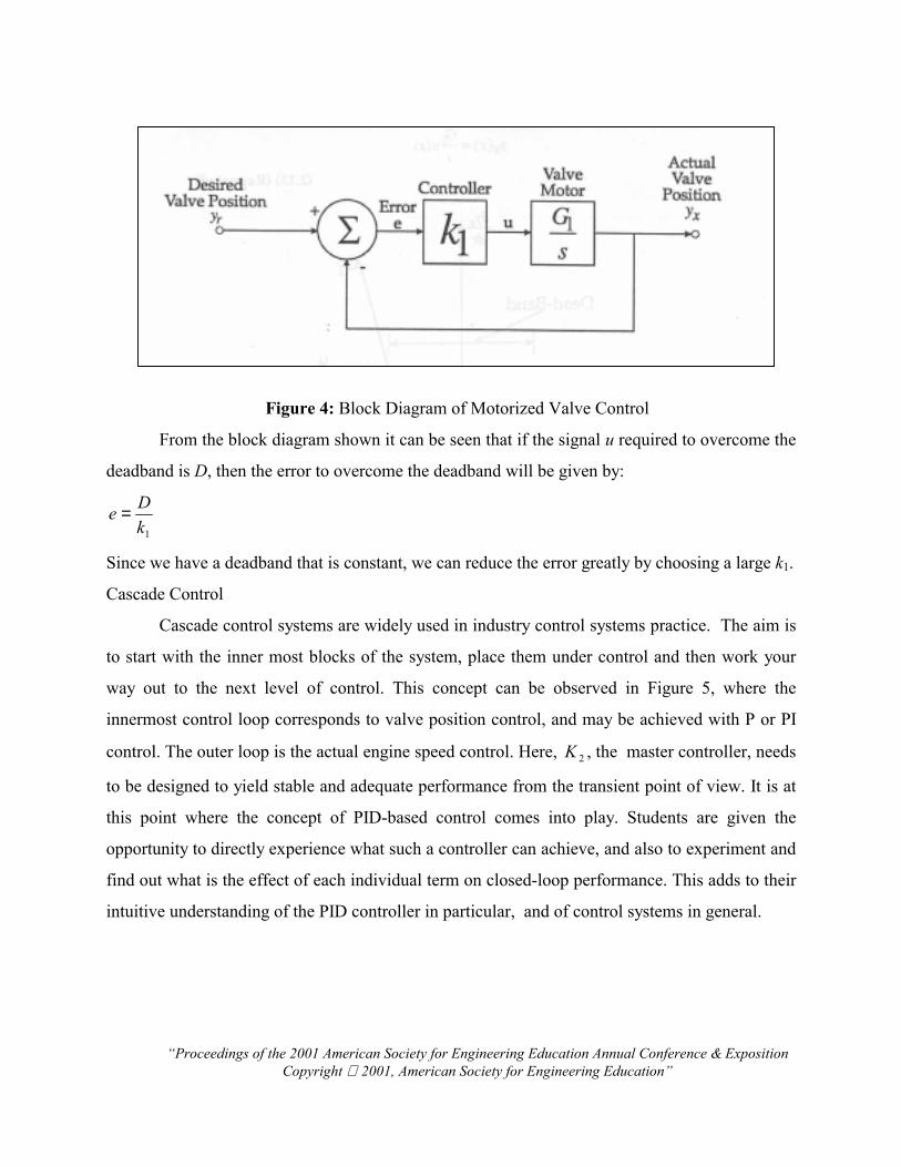
Figure 4: Block Diagram of Motorized Valve Control

From the block diagram shown it can be seen that if the signal u required to overcome the

deadband is D, then the error to overcome the deadband will be given by:

1kDe =

Since we have a deadband that is constant, we can reduce the error greatly by choosing a large k1.

Cascade Control

Cascade control systems are widely used in industry control systems practice. The aim is

to start with the inner most blocks of the system, place them under control and then work your

way out to the next level of control. This concept can be observed in Figure 5, where the

innermost control loop corresponds to valve position control, and may be achieved with P or PI

control. The outer loop is the actual engine speed control. Here, 2K , the master controller, needs

to be designed to yield stable and adequate performance from the transient point of view. It is at

this point where the concept of PID-based control comes into play. Students are given the

opportunity to directly experience what such a controller can achieve, and also to experiment and

find out what is the effect of each individual term on closed-loop performance. This adds to their

intuitive understanding of the PID controller in particular, and of control systems in general.


Figure 5: Engine speed control block diagram

Experiment 2: DC Motor Control Experiment

The plant is to control a DC motor manufactured by Feedback, Inc. The objective is to

achieve motor speed control that performs well under different loads using Feedback's Analog

Unit 33-110 board to create different circuits.

The Mechanical Unit contains a power amplifier that drives the motor from an analogue

or switched input. The motor’s output rotational speed undergoes a 32:1 belt reduction, and it

contains a magnetic brake to simulate a load, as well as a tachogenerator which is used as an

analogue speed transducer. Moreover, the system contains a brake disk with tracks on it. The

motor has a two-phase pulse train that reads a digital output from the brake disk and displays it.

The output shaft carries analogue (potentiometer) and digital (64 location Gray code) angle

transducers (we’re concerned with analogue signals here, but we could also use the digital signal

with the data acquisition card). Finally, the system contains a simple signal generator to provide

low frequency test signals, sine, square, and triangular waves. Figure 6 contains a schematic

diagram of the system.

The Analogue Unit connects to the Mechanical Unit through a 34-way ribbon cable

which carries all power supplies and signals enabling the normal circuit interconnections to be

made on the Analogue Unit using the 2mm patching leads provided. The Analogue Unit is used

to implement the control system. It allows to generate an input, modify the signal, send it to the

motor, and receive the output from the motor.

ye(t)

K1Air

ValveEngineΣK2Σ

e1(t) e2(t)

MasterController

SlaveController

re(t)

rv(t)

yv(t)

- -

u(t)


Figure 6: The DC Motor Experiment: Feedback Mechanical Unit

Controlling the Motor

The motor (Mechanical Unit) can be modeled as a simple DC motor as shown in Figure 7. In

Figure 7: Schematic of the DC Motor

Figure 7, Va(t) is the armature voltage, Ia is the armature current, θm is the shaft angle, θm’ is the

rotation velocity, Jm is the rotor inertia, b is the friction coefficient and Tl is the load torque

(disturbance).

+Va(t) _

DC motor

T θm

bθm’ Tl

Jm


The closed loop system can be represented by the following block diagram:

Figure 8: Control block diagram for the DC Motor

The basic goal of our control system is to enable the system to maintain a certain speed

regardless of the load placed upon it. We can accomplish this by using negative feedback

control. The feedback allows our system to calculate error and provide control that will

compensate for different loads. Here, as with the previous experiment, students are able to

experiment with PID control to achieve a satisfactory speed regulation. In particular, they are

able to observe, by experimenting, the increased disturbance rejection capabilities of the closed-

loop system versus the open-loop, unregulated one, and in particular of a closed-loop system that

uses a PID controller. By using the integral term they learn the real meaning of system type, and

how the integrator is able to provide zero steady state error, as opposed to a simple proportional

controller. Finally, the derivative term allows for a better transient performance, and students

acquire a first-hand experience of the actual meaning of the theory taught in the classroom.

Experiment 3: Feedback Process Control

The Level/Flow Process Control System will be used to study basic characteristics of

Proportional (P) and Proportional-Integral-Derivative (PID) control. The focus of the

experiments are on comparing (P) and (PI) control. Students observe the effect of controller gain

on steady state offset using P control and investigate the effect of controller parameters on the

dynamic response of the system for PI control. The experiments described in this paper use Level

Control experiments to illustrate the effect of the controller parameters on the dynamic response

of the closed loop system. The level control system is shown in Figure 1. A tank is fed with an

inlet flowrate (Fin having dimension volume/time) by a pump. A float level sensor (LS),

transmitter (LT) and controller (LC) are used to maintain the liquid level (h) close to the setpoint

Speed (y)Refspeed (r)

Controller+

_Motor

r-y=e


(hs) by adjusting flow rate out of the tank (Fout) via the control valve. The controller output

signal is based on the error, the difference between the process variable signal from the

transmitter and the setpoint hs. There are four experiments on process control that we describe.

Figure 9: The process level control system (previous paragraph describes the labels)

Disturbance rejection

The first two experiments focus on disturbance rejection. Students impose a 200 mL

pulse disturbance on the feed to the tank, and observe the dynamic response of the liquid level.

Recall from the PID system equation that K1 is the proportional gain, K2 is the derivative gain

and K3 is the integral gain.

Experiment 3 (a): Disturbance Rejection, Proportional-only control. Students investigate

the effect of controller gain K1 on the dynamic response of the system by varying the gain

between 0.1 and 0.25. At the end of the experiment, students should be able to explain the effect

of an increase in controller gain on the steady-state offset and dynamic response of the system.

They should be able to identify the controller gain that results in an oscillatory response. The

dynamic response of the liquid level to a disturbance with P-only control is shown in Figure 10.

hs

LS

F in

F o u t

h

L C

LT


2

4

6

8

10

12

14

0 5 10 15 20 25 30 35Time (s)

Setp

oint

/Pro

cess

Var

iabl

e (m

A

SetpointProcess Variable, K1=0.147Process Variable, K1=0.10Process Variable,K1=0.25

Figure 10: Effect of proportional controller gain on disturbance rejection

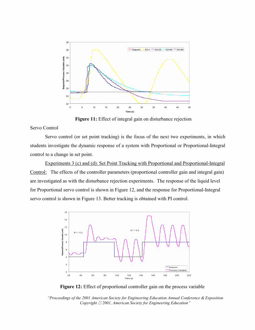
Experiment 3 (b): Disturbance Rejection, Proportional-Integral Control: Students

investigate the effect of reset time (equivalent to integral gain K2) on the dynamic response of the

system by varying the reset time K2 between 40 and 100 s for a range of proportional gain K1. At

the end of the experiment, students should be able to explain the effect of an increase in reset

time on the dynamic response of the system. They should be able to explain how reset time

impacts the speed (or sluggishness) of the response as well as the frequency of oscillations. The

dynamic response of the liquid level to a disturbance with P-I control is shown in Figure 11.


22

24

26

28

30

32

34

36

38

0 5 10 15 20 25 30 35 40 45 50

Time (s)

Setp

oint

/Pro

cess

Var

iabl

e (m

A)

Setpoint K2=1 K2=20 K2=60 K2=80

Figure 11: Effect of integral gain on disturbance rejection

Servo Control

Servo control (or set point tracking) is the focus of the next two experiments, in which

students investigate the dynamic response of a system with Proportional or Proportional-Integral

control to a change in set point.

Experiments 3 (c) and (d): Set Point Tracking with Proportional and Proportional-Integral

Control: The effects of the controller parameters (proportional controller gain and integral gain)

are investigated as with the disturbance rejection experiments. The response of the liquid level

for Proportional servo control is shown in Figure 12, and the response for Proportional-Integral

servo control is shown in Figure 13. Better tracking is obtained with PI control.

0

2

4

6

8

10

12

14

16

20 40 60 80 100 120 140 160 180 200 220Tim e (s)

Setp

oint

/Pro

cess

Var

iabl

e (m

A)

SetpointProcess Variable

K1 = 0.2K1 = 0.5

Figure 12: Effect of proportional controller gain on the process variable


1 5

1 7

1 9

2 1

2 3

2 5

2 7

2 9

3 1

3 3

0 5 0 1 0 0 1 5 0 2 0 0 2 5 0 3 0 0 3 5 0 4 0 0 4 5 0T im e (s )

Setp

oint

/Pro

cess

Var

iabl

e (m

A)

P ro c e s s V a r ia b leS e tp o in t

K 2 = 4 0K 1 = 0 .0 5

K 2 = 2 0K 1 = 0 .0 5

K 2 = 6 0K 1 = 0 .0 5

Figure 13: Effect of integral gain on the process variable

Summary

This NSF-funded project is progressing well at Rowan. We have described

multidisciplinary control experiments on PID control. The experiments allow the students to gain

a better grasp of the PID concept. Students improve their communication skills by writing

laboratory reports.

References

1. N. A. Kheir, K. J. Astrom, D. Auslander, K. C. Cheok, G. F. Franklin, M. Masten and M.

Rabins, “Control systems engineering education,” Automatica, volume 32, pp. 147-166,

1996.

2. R. C. Dorf and R. H. Bishop, Modern Control Systems, Addison-Wesley Longman, 2001.

3. M. F. Aburdene, E. J. Mastascusa, D. S. Schuster and W. J. Snyder, “Computer controlled

laboratory experiments”, Computer Applications in Engineering Education, volume 4, pp.

27-33, 1996.

4. R. Shoureshi, “A course on microprocessor based control systems”, IEEE Control Systems

Magazine, pp. 39-42, June 1992.

5. K. J. Astrom and M. Lundh, “Lund control program combines theory and hands-on

experience”, IEEE Control Systems Magazine, pp. 22-30, June 1992.


6. M. T. Hagan and C. D. Latino, “A modular control systems laboratory”, Computer

Applications in Engineering Education, volume 3, pp. 89-96, 1995.

7. U. Ozguner, “Three course control laboratory sequence”, IEEE Control Systems Magazine,

pp. 14-18, April 1989.

8. M. Mansour and W. Schaufelberger, “Software and laboratory experiments using computers

in control education”, IEEE Control Systems Magazine, pp. 19-24, April 1989.

9. J. A. Newell, A. J. Marchese, R. P. Ramachandran, B. Sukumaran and R. Harvey,

“Multidisciplinary Design and Communication: A Pedagogical Vision'', International

Journal of Engineering Education, Vol. 15, No. 5, pp. 376-382, 1999.

10. K. Jahan, R. A. Dusseau, R. P. Hesketh, A. J. Marchese, R. P. Ramachandran, S. A

Mandayam and J. L. Schmalzel, “Engineering Measurements in the Freshman Engineering

Clinic at Rowan University”, ASEE Annual Conference and Exposition, Seattle, Washington,

Session 1326, June 28-July 1, 1998.

11. A. J. Marchese, J. A. Newell, R. P. Ramachandran, B. Sukumaran, J. L. Schmalzel and J.

Marriappan, “The Sophomore Engineering Clinic: An Introduction to the Design Process

Through a Series of Open Ended Projects”, ASEE Annual Conference and Exhibition,

Charlotte, North Carolina, Session 2225, June 20-23, 1999.

12. L. M. Head, G. Canough and R. P. Ramachandran, “Design of a Robust and Low Cost Solar

Lantern as a One Semester Project'', ASEE Annual Conference and Exhibition, St. Louis,

Missouri, Session 2793, June 18--21, 2000.

Acknowledgement

The authors wish to acknowledge that this work was supported by an NSF CCLI grant (DUE #

9950882).

Biography

Ravi P. Ramachandran is an Associate Professor in the Department of Electrical and Computer

Engineering at Rowan University. He received his Ph.D. from McGill University in 1990 and has

worked at AT&T Bell Laboratories and Rutgers University prior to joining Rowan.


Stephanie Farrell is an Associate Professor in the Department of Chemical Engineering at Rowan

University. She received her Ph.D. degree in 1996 from the New Jersey Institute of Technology.

She was on the faculty at Louisiana Tech University prior to joining Rowan.

Raul Ordonez is an Assistant Professor in the Department of Electrical and Computer

Engineering at Rowan University. He received his Ph.D. from Ohio State University in 1999. His

research interests include nonlinear control and robotics.

Zenaida Otero Gephardt is Associate Professor of Chemical Engineering at Rowan University

where she has also served as Assistant Dean and Director of Engineering. She holds a Ph.D. in

chemical engineering from the University of Delaware and is a licensed professional engineer.

Her expertise is in process optimization, statistical analysis and experimental design. She has

worked with supercritical fluids and particle technology.

Hong Zhang obtained his Ph.D. from the GRASP lab of the University of Pennsylvania in 2000.

Thereafter, he joined the Mechanical Engineering Department of Rowan University as an

Assistant Professor. His research interests includes robot motion planning, visual servo control

and nonlinear control.

multidiscplinary control experiments based on the

Documents