Multichannel Singular Spectrum Analysis in the Estimates of Common Environmental Effects

Affecting GPS Observations

MARTA GRUSZCZYNSKA,1 SEVERINE ROSAT,2 ANNA KLOS,1 MACIEJ GRUSZCZYNSKI,1 and JANUSZ BOGUSZ1

Abstract—We described a spatio-temporal analysis of envi-

ronmental loading models: atmospheric, continental hydrology, and

non-tidal ocean changes, based on multichannel singular spectrum

analysis (MSSA). We extracted the common annual signal for 16

different sections related to climate zones: equatorial, arid, warm,

snow, polar and continents. We used the loading models estimated

for a set of 229 ITRF2014 (International Terrestrial Reference

Frame) International GNSS Service (IGS) stations and discussed

the amount of variance explained by individual modes, proving that

the common annual signal accounts for 16, 24 and 68% of the total

variance of non-tidal ocean, atmospheric and hydrological loading

models, respectively. Having removed the common environmental

MSSA seasonal curve from the corresponding GPS position time

series, we found that the residual station-specific annual curve

modelled with the least-squares estimation has the amplitude of

maximum 2 mm. This means that the environmental loading

models underestimate the seasonalities observed by the GPS sys-

tem. The remaining signal present in the seasonal frequency band

arises from the systematic errors which are not of common envi-

ronmental or geophysical origin. Using common mode error

(CME) estimates, we showed that the direct removal of environ-

mental loading models from the GPS series causes an artificial loss

in the CME power spectra between 10 and 80 cycles per year.

When environmental effect is removed from GPS series with

MSSA curves, no influence on the character of spectra of CME

estimates was noticed.

Key words: Multichannel singular spectrum analysis, sea-

sonal signals, GPS, environmental loading models.

1. Introduction

Seasonal changes are a component part of the

Global Positioning System (GPS) position time ser-

ies, especially the vertical direction (Blewitt and

Lavallee 2002; Collilieux et al. 2007). In most cases,

those variations result from real geophysical phe-

nomena which deform the Earth’s surface. They are

broadly explained and modelled by environmental

loading effects (van Dam and Wahr 1998; Jiang et al.

2013). Atmospheric (van Dam and Wahr 1987),

hydrological (van Dam et al. 2001) and non-tidal

ocean (van Dam et al. 2012) loadings are the most

important contributors of seasonal variations to many

GPS stations in different parts of the world. The

appropriate models can be removed directly from the

GPS position time series to reduce the influence they

might have on the observed displacements. This

approach has proved to decrease the root mean square

(RMS) of the GPS position time series (Jiang et al.

2013). However, according to Santamarıa-Gomez

and Memin (2015), such an approach reduces only

the amplitude of white noise of the GPS position time

series. Klos et al. (2017) showed that the direct

removal of environmental loading models from the

GPS observations causes the evident change in the

power spectrum density of noise for frequencies

between 4 and 80 cycles per year (cpy).

Beyond real geophysical origins, seasonal chan-

ges in the GPS position time series can be also

generated by systematic errors (Ray et al. 2008) or by

spurious effects (Penna et al. 2007). Both can influ-

ence permanent stations individually or be similar for

stations situated not far from each other.

As shown by Dong et al. (2002), both the GPS

position time series and the environmental loading

Electronic supplementary material The online version of this

article (https://doi.org/10.1007/s00024-018-1814-0) contains sup-

plementary material, which is available to authorized users.

1 Faculty of Civil Engineering and Geodesy, Military

University of Technology, Warsaw, Poland. E-mail:

marta.gruszczynska@wat.edu.pl2 Institut de Physique du Globe de Strasbourg, UMR 7516,

Universite de Strasbourg/EOST, CNRS, Strasbourg, France.

Pure Appl. Geophys. 175 (2018), 1805–1822

� 2018 The Author(s)

This article is an open access publication

https://doi.org/10.1007/s00024-018-1814-0 Pure and Applied Geophysics

models contain the common seasonal signal which

characterizes the data from a certain region of the

world. Freymueller (2009), Tesmer et al. (2009) and

Bogusz et al. (2015a) proposed to employ stacking

and clustering methods to estimate regional mean

annual oscillations from the time series and to group

them from a regional signal. They all proved that the

neighbouring stations are characterized by a similar

seasonal signal.

Few methods such as Singular Spectrum Analysis

(SSA), Wavelet Decomposition (WD) and Kalman

Filter (KF) have been already used to retrieve station-

dependent time-varying curves from the GPS position

time series (Chen et al. 2013; Gruszczynska et al.

2016; Didova et al. 2016; Klos et al. 2018a). How-

ever, neither of them is able to separate real and

spurious effects from the GPS data. Lately, multi-

channel singular spectrum analysis (MSSA) was

proposed by Walwer et al. (2016) for stations situated

close to each other. They demonstrated that MSSA is

able to model the common seasonal signal in the GPS

position time series. Zhu et al. (2016) used the MSSA

approach to investigate the inter-annual oscillations

in glacier mass change estimated from gravity

recovery and climate experiment (GRACE) data in

Central Asia. Gruszczynska et al. (2017) compared

the MSSA-, SSA- and least-squares estimation-

derived seasonal signals. They showed that the sea-

sonal signals detected by MSSA are not affected by

noise as much as the SSA-derived oscillations. It was

explained by the fact that SSA estimates individually

fitted curve for the analysed station, while MSSA

takes into account the common effects which are

observed by few neighbouring GPS stations. As the

noise is mainly a station-specific signal, MSSA

curves will not be affected by it as much as SSA

curves.

To indicate the signals which arise from real

geophysical effects, Klos et al. (2017) proposed a

two-stage solution based on Improved Singular

Spectrum Analysis (ISSA, Shen et al. 2015). When

applied for loading models from an individual station,

the time-varying seasonal signals from environmental

atmospheric, hydrological and non-tidal ocean load-

ings were extracted, causing the character of the

stochastic part characterized a power-law noise (e.g.

Williams 2003; Bogusz and Kontny 2011;

Santamarıa-Gomez et al. 2011; Klos et al. 2016; Klos

and Bogusz 2017) remained intact. In this research,

we assumed that the GPS position time series should

not be affected by the high frequency part of envi-

ronmental loadings series as we did not know if GPS

observations to a large extent are influenced by the

environmental effects. Therefore, we focused on the

common environmental effect in a form of time-

varying annual curve which is observed at the GPS

permanent stations and proposed its modelling with-

out any alteration in the character of the stochastic

part of the time series.

Beyond seasonal signals, the GPS-derived series

are also characterized by common mode error

(CME), being a sum of the systematic errors

(Wdowinski et al. 1997; Nikolaidis 2002; King et al.

2010). Mismodeling of the earth orientation param-

eters (EOPs), mis- or un-modelled large-scale

atmospheric and hydrologic effects or small scale

crust deformations, all increase spatial correlations

between individual series. CME can be easily esti-

mated using stacking (Wdowinski et al. 1997;

Nikolaidis 2002), spatial filtering (Marquez-Azua and

DeMets 2003) or orthogonal transformation func-

tions. The latter is considered to be the most effective

in reflecting the real nature of CME (Dong et al.

2006). Yuan et al. (2008) proved that a direct removal

of surface mass loadings can significantly reduce the

power-law noise. However, they did not investigate

to what extent the properties of CME are affected. As

was shown by Klos et al. (2017) a part of the power is

removed when real geophysical effects are consid-

ered by direct subtraction of environmental loading

models. We presumed that the CME values may also

be affected by such removal.

In this paper, we proposed the spatial analysis of

environmental loading models based on MSSA to

extract the common annual signal for 16 different

sections related to the climate zones (i.e. equatorial,

arid, warm, snow, polar) and continents. We then

modelled with MSSA the time-varying seasonal sig-

nal from environmental loading models and

subtracted them from the GPS height time series.

This was aimed to remove real geophysical changes

from the GPS data leaving the noise character of time

series unchanged. The benefits of this approach were

presented for CME estimates which should not

1806 M. Gruszczynska et al. Pure Appl. Geophys.

include the environmental effects, as they were

removed by the MSSA approach and, most impor-

tantly, no influence on CME character should be

noticed.

2. Methodology

In this section, we provided a detailed description

of the data and the methodology we used. Data

included the environmental loading models and the

GPS height time series collected at 229 stations from

around the globe. The division into 16 different sec-

tions according to the climate classification is also

presented.

2.1. Data

We employed the GPS position time series from

229 stations distributed globally (Fig. 1). Daily time

series were derived from network solution

(Rebischung et al. 2016) produced by the Interna-

tional GNSS Service (IGS). They contributed to the

latest realization of the International Terrestrial

Reference System (namely ITRF2014; Altamimi

et al. 2016). We selected the vertical components

which were not shorter than 10 years. To remove

offsets, we used the epochs defined by IGS in station

log-files with the manual inspection of the series.

Outliers were removed with the Interquartile Range

(IQR) approach.

Under the Synthesis Report about Climate Change

published by Intergovernmental Panel on Climate

Change (IPCC), a region’s climate is generated by the

system, which has five main components: atmo-

sphere, hydrosphere, cryosphere, lithosphere, and

biosphere (AR4 SYR Synthesis Report Annexes,

http://www.ipcc.ch, retrieved on 2017-06-28).

According to this report, we investigated environ-

mental loading effects which may be correlated

within climate zones. Therefore, 229 stations were

divided into sixteen sections (Table 1, and Table S1

Koppern-GeigerClimate Classification:

B: AridC: Warm temperateD: SnowE: Polar

A: Equatorial

Figure 1World Map of Koppen–Geiger Climate Classification with the GPS permanent stations considered in this analysis plotted in grey. The A:

Equatorial, B: Arid, C: Warm temperate, D: Snow and E: Polar climate zones are presented in red, yellow, green, turquoise and blue,

respectively

Vol. 175, (2018) Common Environmental Effects in GPS data 1807

in Supplementary Materials) which are associated

with these zones and also with different continents.

We used the Koppen–Geiger Climate Classification

(Rubel and Kottek 2010) to divide stations according

to similar conditions. Then, the time-varying curves

were modelled separately for each section.

The atmospheric, hydrological and non-tidal ocean

loading models in Centre-of-Figure (CF) frame were

employed. Atmospheric loadings were determined

from ERA interim (ECMWF Reanalysis) model (Dee

et al. 2011). Non-tidal ocean loadings were estimated

from Estimation of the Circulation and Climate of the

Ocean version 2 (ECCO2) (Menemenlis et al. 2008)

ocean bottom pressure model. Hydrological loading

(soil moisture and snow) was estimated from modern

era-retrospective analysis (MERRA) land model (Re-

ichle et al. 2011). These environmental loadings were

developed at the Ecole et Observatoire des Sciences de

la Terre (EOST) loading service available at http://

loading.u-strasbg.fr/.

Since the ECCO2model and the GPS position time

series are sampled every day, the ERAIN andMERRA

models were decimated into a daily sampling using a

low-pass filter. One of the requirements of the MSSA

approach is a common time span of data sets; therefore,

we selected a period from 1st January 1994 to 14th

February 2015 to be common for all stations. In this

study, we focused on the vertical component for which

the environmental loading is themost significant (Dach

et al. 2011; van Dam et al. 2012).

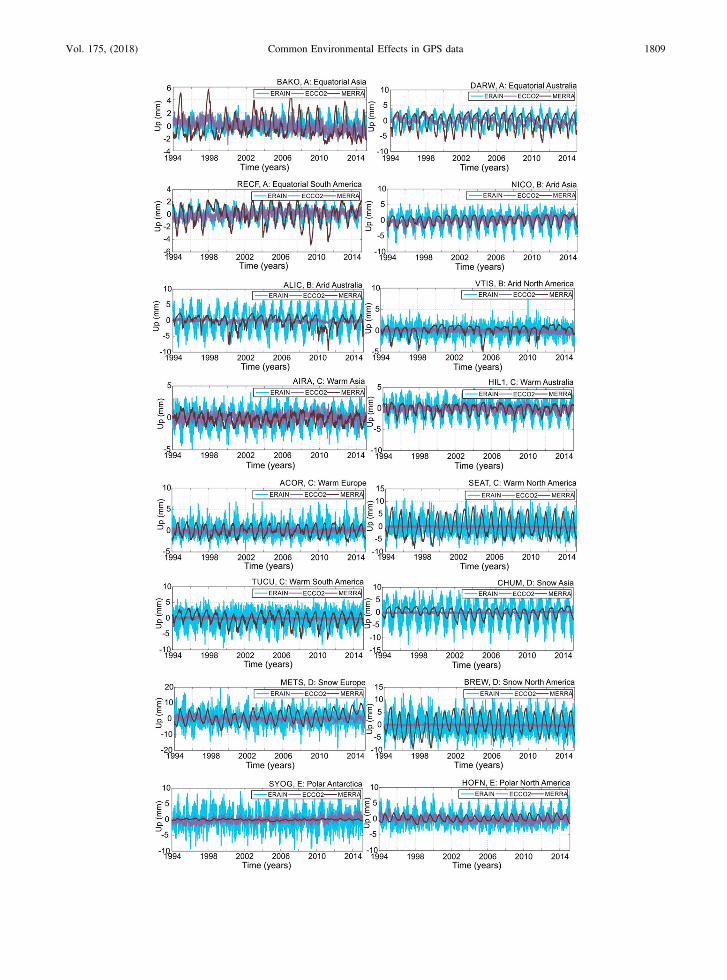
Figure 2 presents series of environmental loadings

for selected stations from each section to show the time

variability we may be dealing with. Depending on the

section considered, the atmospheric, hydrological and

non-tidal ocean effects can be larger than others.

According to BAKO (Cibinong, Indonesia), ALIC

(Alice Springs, Australia), BREW (Brewster, United

States) and TUCU (San Miguel de Tucuman, Argen-

tina) stations, we may notice that the amplitude of

MERRA model significantly varies over time with

maximum peak-to-peak amplitude being equal to

about 5, 7, 10 and 4 mm, respectively. Similarly, we

may see in atmospheric loading at ACOR (A Coruna,

Spain) and SEAT (Seattle, United States) stations that

the peaks differ by 5 and 4 mm, respectively. DARW

(Darwin, Australia) station is characterized by ECCO2

model with time-varying amplitude of about 2 mm.

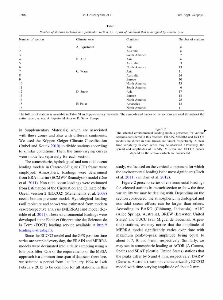
Table 1

Number of stations included in a particular section, i.e. a part of continent that is assigned by climate zone

Number of section Climate zone Continent Number of stations

1 A: Equatorial Asia 6

2 Australia 6

3 South America 7

4 B: Arid Asia 6

5 Australia 3

6 North America 13

7 C: Warm Asia 11

8 Australia 24

9 Europe 30

10 North America 33

11 South America 6

12 D: Snow Asia 17

13 Europe 18

14 North America 25

15 E: Polar Antarctica 13

16 North America 11

The full list of stations is available in Table S1 in Supplementary materials. The symbols and names of the sections are used throughout the

entire paper, as, e.g. A: Equatorial Asia or D: Snow Europe

Figure 2The selected environmental loading models presented for various

sections considered in this research. ERAIN, MERRA and ECCO2

models are shown in blue, brown and violet, respectively. A clear

time variability in each series may be observed. Obviously, the

spread and amplitudes of ERAIN, MERRA and ECCO2 curves

depend on the sections which are considered

c

1808 M. Gruszczynska et al. Pure Appl. Geophys.

Vol. 175, (2018) Common Environmental Effects in GPS data 1809

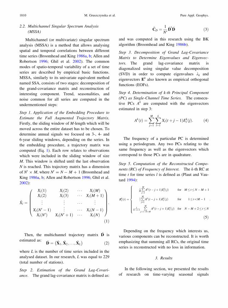
2.2. Multichannel Singular Spectrum Analysis

(MSSA)

Multichannel (or multivariate) singular spectrum

analysis (MSSA) is a method that allows analysing

spatial and temporal correlations between different

time series (Broomhead and King 1986a, b; Allen and

Robertson 1996; Ghil et al. 2002). The common

modes of spatio-temporal variability of a set of time

series are described by empirical basic functions.

MSSA, similarly to its univariate equivalent method

named SSA, consists of two stages: decomposition of

the grand-covariance matrix and reconstruction of

interesting component. Trend, seasonalities, and

noise common for all series are computed in the

undermentioned steps:

Step 1. Application of the Embedding Procedure to

Estimate the Full Augmented Trajectory Matrix.

Firstly, the sliding window of M-length which will be

moved across the entire dataset has to be chosen. To

determine annual signals we focused on 3-, 4- and

6-year sliding windows, depending on the series. In

the embedding procedure, a trajectory matrix was

computed (Eq. 1). Each row relates to observations

which were included in the sliding window of size

M. This window is shifted until the last observation

N is reached. This trajectory matrix has a dimension

of N0 9 M, where N0 = N - M ? 1 (Broomhead and

King 1986a, b; Allen and Robertson 1996; Ghil et al.

2002):

~Xl ¼

Xl 1ð Þ Xl 2ð Þ � � � Xl Mð ÞXl 2ð Þ Xl 3ð Þ � � � Xl M þ 1ð Þ... ..

.� � � ..

.

Xl N 0 � 1ð Þ ...

� � � Xl N � 1ð ÞXl N 0ð Þ Xl N 0 þ 1ð Þ � � � Xl Nð Þ

0BBBBB@

1CCCCCA:

ð1Þ

Then, the multichannel trajectory matrix ~D is

estimated as: ~D ¼ ~X1; ~X2; . . .; ~XL

� �ð2Þ

where L is the number of time series included in the

analysed dataset. In our research, L was equal to 229

(total number of stations).

Step 2. Estimation of the Grand Lag-Covari-

ance. The grand lag-covariance matrix is defined as:

~CD ¼ 1

N 0~D

t ~D ð3Þ

and was computed in this research using the BK

algorithm (Broomhead and King 1986b).

Step 3. Decomposition of Grand Lag-Covariance

Matrix to Determine Eigenvalues and Eigenvec-

tors. The grand lag-covariance matrix is

diagonalized using singular value decomposition

(SVD) in order to compute eigenvalues kk and

eigenvectors Ek also known as empirical orthogonal

functions (EOFs).

Step 4. Determination of k-th Principal Component

(PC) as Single-Channel Time Series. The consecu-

tive PCs Ak are computed with the eigenvectors

estimated in step 3:

AkðtÞ ¼XM

j¼1

XL

l¼1

Xlðt þ j � 1ÞEkl ðjÞ: ð4Þ

The frequency of a particular PC is determined

using a periodogram. Any two PCs relating to the

same frequency as well as the eigenvectors which

correspond to those PCs are in quadrature.

Step 5. Computation of the Reconstructed Compo-

nents (RC) of Frequency of Interest. The k-th RC at

time t for time series l is defined as (Plaut and Vau-

tard 1994):

Rkl tð Þ ¼

1M

PMj¼1

Ak t � j þ 1ð ÞEkl jð Þ for M � t �N � M þ 1

1i

PMj¼1

Ak t � j þ 1ð ÞEkl jð Þ for 1� t\M � 1

1N�iþ1

PMj¼1�NþM

Ak t � j þ 1ð ÞEkl jð Þ for N � M þ 2� t�N

8>>>>>>>>><>>>>>>>>>:

:

ð5Þ

Depending on the frequency which interests us,

various components can be reconstructed. It is worth

emphasizing that summing all RCs, the original time

series is reconstructed with no loss in information.

3. Results

In the following section, we presented the results

of research on time-varying seasonal signals

1810 M. Gruszczynska et al. Pure Appl. Geophys.

estimated with MSSA, separately for environmental

loadings in each considered section. Then, we anal-

ysed the residuals of the GPS height time series

obtained by subtraction of the common time-varying

annual curves from data. Finally, we estimated the

CME values to decide on the efficiency of the pro-

posed approach. We aimed to propose MSSA as an

alternative method to remove the common environ-

mental effect from the GPS position time series

without affecting their stochastic characters.

3.1. Common Seasonal Signals Estimated

from Environmental Loadings

Common seasonal signals were estimated with

MSSA from environmental loadings separately for

sixteen considered sections (Fig. 3) and then summed

to each other for the time span of 1.01.1994-

14.02.2015. Residuals of the GPS height time series

were produced by de-trending each of them and by

removing the common annual signal for epochs

corresponding to GPS observations. These residuals

were then subjected to CME estimates. In this

research, we intentionally focused on annual period,

as the percentage of total variance of time series

explained by modes of annual signal is much higher

than the variance explained by any other pair of

modes (Gruszczynska et al. 2016).

The principal components which correspond to

the same frequency describe the common character of

the employed time series. In other words, each

individual PC constitutes a pattern of the common

signal. PCs and eigenvectors of the annual period

were combined to estimate the k-th RC to determine

common oscillations for stations in a particular

section, not of the individual station. The percentage

of variance explained by the common signal is

strictly related to the variance of entire time series

estimated including trend, noise and other seasonal

signals. It can be only interpreted in the context of all

the time series common components variability. As

an example, we can provide a series with the

significant amplitude of the common annual signal,

and the common trend, noise, and other seasonalities

being also significant. Then, the contribution of the

common annual signal is comparatively low in

relation to the remaining components identified

through the MSSA procedure. On the contrary, if

the variance of trend, noise and other seasonalities is

small, the total variance of data explained by the

annual curve will be significant and large.,

From Fig. 4, we can notice that for ERAIN

loading model, two first PCs are always related to

common annual signals explaining between 4 and

80% of the total variance of data. If the percentage of

variance explained by the annual signal is relatively

low, the higher is the variance that represents the sum

of the other time series components (trend, noise, and

other seasonalities). For 7 sections, i.e. B: Arid North

America, C: Warm Europe, C: Warm North and

South America, D: Snow Europe, D: Snow North

America and E: Polar Antarctica, the variance

explained by the annual signal is relatively low in

comparison to the variance explained by other modes

and varies between 4 and 8%. For other sections, this

variance is much higher and ranges 31-80%.

For MERRA loading model, the two first PCs

always combine to annual signal. The variance

explained by it varies between 31 and 83% of total

variance of data. Zones as B: Arid Australia, B: Arid

North America and C: Warm Australia are charac-

terized by a high contribution of lower modes into the

total percentage of variance equal to nearly 70% at

maximum. For other sections, this percentage

Station 1ERAIN

Station 3ERAIN

Station 2ERAIN

Station nERAIN

Station 1MERRA

Station 3MERRA

Station 2MERRA

Station nMERRA

Station 1ECCO2

Station 3ECCO2

Station 2ECCO2

Station nECCO2

For each section

...

......

...

...

...

......

...

......

Figure 3An idea of MSSA employed for a particular section and

environmental model. The common annual signal was estimated

based on time series included in the considered section, separately

either for each section or each loading model. Then, the common

annual signals estimated for ERAIN, MERRA and ECCO2 were

summed to each other to reveal the common environmental effect

which affects the GPS position time series

Vol. 175, (2018) Common Environmental Effects in GPS data 1811

0

10

20

30

40

Annual: PC 1-2

MERRA

Annual: 83 %

0

5

10

15

0 5 10 15

No. of mode0 5 10 15

No. of mode0 5 10 15

No. of mode

0 5 10 15

No. of mode0 5 10 15

No. of mode0 5 10 15

No. of mode

0 5 10 15

No. of mode0 5 10 15

No. of mode0 5 10 15

No. of mode

0 5 10 15

No. of mode0 5 10 15

No. of mode0 5 10 15

No. of mode

0 5 10 15

No. of mode0 5 10 15

No. of mode0 5 10 15

No. of mode

Annual: PC 1-2

ECCO2

Annual: 29 %

0

10

20

30

40

Annual: PC 1-2

ERAIN

Annual: 80 %

A: Equatorial Asia

0

4

8

12

16

0

10

20

30

40

0

10

20

30 MERRAECCO2 ERAIN

Annual: PC 1-2Annual: 68 %

Annual: PC 1-2Annual: 34 %

Annual: PC 1-2Annual: 72 %

A: Equatorial Australia

0

2

4

6

8

0

10

20

0

10

20

30

MERRAECCO2 ERAIN

Annual: PC 1-2Annual: 77 %

Annual: PC 2-3Annual: 11 %

Annual: PC 1-2Annual: 48 %

A: Equatorial South America

0

4

8

12

0

10

20

30

40

0

10

20

30MERRAERAINECCO2

Annual: PC 1-2Annual: 65 %

Annual: PC 1-2Annual: 24 %

Annual: PC 1-2Annual: 74 %

B: Arid Asia

0

4

8

12

0

10

20

30

0

4

8

12

16

Var

ianc

e (%

)V

aria

nce

(%)

Var

ianc

e (%

)V

aria

nce

(%)

Var

ianc

e (%

)

MERRAECCO2 ERAIN

Annual: PC 1-2Annual: 31 %

Annual: PC 1-2Annual: 26 %

Annual: PC 1-2Annual: 65 %

B: Arid Australia

1812 M. Gruszczynska et al. Pure Appl. Geophys.

explains between 60 and 83% and obviously is

location dependent.

For ECCO2 loading model, the 2nd and 3rd PCs

from sections: A: Equatorial South America, C:

Warm North America, D: Snow Asia, and D: Snow

North America are related to the common annual

signal, while for 3 sections, namely: B: Arid North

America, E: Polar Antarctica and E: Polar North

America—the 3rd and 4th. For all these cases, first

PCs explain the long-term non-linear trend. As an

example, for E: Polar Antarctica section, the ECCO2

series are characterized by large non-linearity mainly

between 2006 and 2015, while for stations included

in E: Polar North America section, the non-linearity

from 2000 onwards is hardly seen, as the variance

explained by this non-linear trend is comparable to

the annual signal. The long-term trend seen in the

ECCO2 model may result from the Boussinesq

approximation used to create this model (Ponte

et al. 2007). For remaining 9 sections, annual signals

were detected in the 1st and 2nd PCs with the amount

of variance explained by annual curve being signif-

icantly higher than the variance explained by other

modes.

Figure 5 presents the spatial distribution of the

percentage of variance which is explained by a

common annual signal in the vertical direction for

ECCO2, ERAIN and MERRA model, respectively,

for individual stations situated in different sections.

For the non-tidal ocean loading model, the

common annual signal identified using MSSA

accounts for an average of 16% of the total variance

of data. The highest contribution of the annual signal

was noticed for stations situated in A: Equatorial

Australia section, reaching 34%. In Europe, the

annual signal explains approximately 26%, while in

North and South Americas 6 and 9%, respectively.

Common annual oscillations identified using MSSA

for atmospheric loading account for an average of

24% of the total variance of data with the highest

percentage equal to 80, 72 and 74%, respectively, for

stations situated in South Asia, in North Australia and

in Asia. The percentage of variance related to annual

oscillation explains approximately 4% of the total

variance for stations in Europe. The annual signal

estimated using MSSA approach for the hydrological

loading models explains around 68% of the total

variance, proving that local hydrological plays a

significant role in the observed signals. We noticed

that stations situated in Europe are strongly affected

by annual oscillations from hydrological loading,

which accounts for 80%. Those results may be further

used for other research related for example to the

climate studies, but it falls out of the scope of this

paper.

Then, we estimated the RCs for ERAIN, MERRA

and ECCO2 models for all examined stations.

Figure 6 reveals the original MERRA time series

for stations from A: Equatorial Asia section and

common seasonal signal derived by the MSSA

approach. Due to the non-parametric character of

MSSA, we were able to estimate common seasonal

pattern which is not constant over time. From Fig. 6,

we can notice that the maximum amplitude estimated

for A: Equatorial Asia was equal to 5.9 mm at the

beginning of 2007, while the smallest peak was equal

to 4.8 mm in 2002. We compared the common

annual signals estimated with MSSA with those

determined with LSE separately for each loading

model, obtaining maximum difference in peak-to-

peak oscillations of 2.2 mm (or 77% in other words)

at maximum.

Finally, the common seasonal signal estimated

from ERAIN, MERRA, and ECCO2 with MSSA

algorithm was subtracted from the GPS height time

series. Due to numerical artefacts, the environmental

loadings do not account for entire seasonal oscillation

observed by the GPS time series, as pointed the

Introduction section. Therefore, we modelled the

remaining annual oscillations from the residual time

series using the LSE approach. The median amplitude

of the residual annual oscillations estimated for the

229 GPS stations was equal to 1.7 mm. They arose

from the fact that the common annual oscillation

estimated with MSSA did not reflect the entire

seasonal changeability of series due to its spatial

pattern. These residual annual oscillations were

bFigure 4

Percentage of variance explained by individual modes for

environmental loadings for all sections we analysed. The modes

which were used to reconstruct the annual changes are marked in

red. Also, the percentage of variance explained by annual signal is

given in each plot

Vol. 175, (2018) Common Environmental Effects in GPS data 1813

0

4

8

12

16

0

1

2

3

4

0

4

8

12

16

20

0 5 10 15

No. of mode

0 5 10 15

No. of mode

0 5 10 15

No. of mode

0 5 10 15

No. of mode

0 5 10 15

No. of mode

0 5 10 15

No. of mode

0 5 10 15

No. of mode

0 5 10 15

No. of mode

0 5 10 15

No. of mode

0 5 10 15

No. of mode

0 5 10 15

No. of mode

0 5 10 15

No. of mode

0 5 10 15

No. of mode

0 5 10 15

No. of mode

0 5 10 15

No. of mode

MERRAECCO2 ERAIN

Annual: PC 1-2Annual: 37 %

Annual: PC 3-4Annual: 3 %

Annual: PC 1-2

B: Arid North America

Annual: 8 %

0

4

8

12

0

10

20

30

0

10

20

30MERRAERAINECCO2

Annual: PC 1-2Annual: 68 %

Annual: PC 1-2Annual: 25 %

Annual: PC 1-2Annual: 68 %

C: Warm Asia

0

5

10

15

0

4

8

12

16

0

10

20MERRAECCO2 ERAIN

Annual: PC 1-2Annual: 43 %

Annual: PC 1-2Annual: 28 %

Annual: PC 1-2Annual: 35 %

C: Warm Australia

0

10

20

30

40

0

4

8

12

0

1

2MERRAECCO2 ERAIN

Annual: PC 1-2Annual: 82 %

Annual: PC 1-2Annual: 25 %

Annual: PC 1-2Annual: 4 %

C: Warm Europe

0

10

20

0

1

2

3

0

10

20

30

Var

ianc

e (%

)V

aria

nce

(%)

Var

ianc

e (%

)V

aria

nce

(%)

Var

ianc

e (%

)

MERRAERAINECCO2

Annual: PC 1-2Annual: 80 %

Annual: PC 2-3Annual: 5 %

Annual: PC 1-2Annual: 6 %

C: Warm North America

Figure 4continued

1814 M. Gruszczynska et al. Pure Appl. Geophys.

0

1

2

3

4

5

0

2

4

6

8

0

10

20MERRAERAINECCO2

Annual: PC 1-2Annual: 60 %

Annual: PC 1-2Annual: 9 %

Annual: PC 1-2Annual: 8 %

C: Warm South America

0

2

4

6

8

0

10

20

0

10

20

30

Annual: PC 1-2Annual: 66 %

Annual: PC 2-3Annual: 11 %

Annual: PC 1-2Annual: 46 %

D: Snow Asia

0

5

10

15

0

1

2

3

0

10

20

30

40

Annual: PC 1-2Annual: 79 %

Annual: PC 1-2Annual: 28 %

Annual: PC 1-2Annual: 6 %

D: Snow Europe

0

4

8

12

0

1

2

3

4

5

0

10

20

30

40

Annual: PC 1 -2Annual: 75 %

Annual: PC 2 -3Annual: 10 %

Annual: PC 1 -2Annual: 10 %

D: Snow North America

0

10

20

30

40

0

2

4

6

0

10

20

30

0 5 10 15

No. of mode0 5 10 15

No. of mode0 5 10 15

No. of mode

0 5 10 15

No. of mode0 5 10 15

No. of mode0 5 10 15

No. of mode

0 5 10 15

No. of mode0 5 10 15

No. of mode0 5 10 15

No. of mode

0 5 10 15

No. of mode0 5 10 15

No. of mode0 5 10 15

No. of mode

0 5 10 15

No. of mode0 5 10 15

No. of mode0 5 10 15

No. of mode

Var

ianc

e (%

)V

aria

nce

(%)

Var

ianc

e (%

)V

aria

nce

(%)

Var

ianc

e (%

)

Annual: PC 1-2Annual: 61 %

Annual: PC 3-4Annual: 5 %

Annual: PC 1-2Annual: 10 %

E: Polar Antarctica

MERRAERAINECCO2

MERRAERAINECCO2

MERRAERAINECCO2

MERRAERAINECCO2

Figure 4continued

Vol. 175, (2018) Common Environmental Effects in GPS data 1815

subtracted to estimate the series submitted for further

analysis.

3.2. Common Mode Errors

In order to show the main advantage of estimating

the seasonal signal with MSSA, we determined the

Common Mode Error (CME) with the use of the

Principal Component Analysis (PCA) for incomplete

GNSS time series as proposed by Shen et al. (2013).

This procedure was previously successfully applied

by the authors for spatio-temporal analysis of the

GPS position time series (Bogusz et al. 2015b;

Gruszczynski et al. 2016). First, CME was estimated

for residuals after MSSA curves were removed. Then,

CME was estimated for residuals after direct sub-

traction of environmental loading models. The

second approach is nowadays widely used to remove

the environmental effects from the GPS position time

series, while first is a novelty introduced in this paper.

Figure 7 presents the selected stacked power

spectral densities of height time series CME deter-

mined for individual sections after environmental

effect was removed using MSSA-derived annual

curve as well as removed directly from time series.

These results confirm that although the direct

subtraction of environmental loading models from

the GPS position time series may help in removing

the loading effect and in reducing the RMS values, it

causes a change in the character of the stochastic part

of time series leading to an artificial subtraction of

some power in CME. On the other hand, we may

suppose that some part of the Common Mode Error

observed by the GPS sensors arises from environ-

mental influence. However, it has not yet been

considered if the GPS records are sensitive to

environmental influence in the frequency bands

between 10 and 80 cpy. If not, we should not

artificially influence the character of CME by

removal of entire environmental loadings.

From Fig. 7, we may notice that the character of

CME is very similar for both cases for the B: Arid

Australia section. For A: Equatorial Australia, C:

Warm South America, D: Snow Europe, and E: Polar

North America, we can observe that environmental

loading models remove lots of power in a frequency

band between 10 and 80 cpy. Especially, zones as C:

Warm South America and D: Snow Europe are

affected by a large cut in the power, and, therefore, a

change in a character of CME. When MSSA curves

which reveal the common geophysical signal are

removed from the GPS position time series, the

change in power is not observed, which means that

the character of CME remains intact.

Based on the results, we concluded that the

common geophysical signal can be successfully

modelled with the MSSA method and then removed

from the GPS position time series. We showed that

the CME values are not affected by MSSA estimates,

which makes it to be an effective approach to

investigate and/or subtract a common large-scale

environmental effect in the GPS position time series.

4. Discussion and Conclusions

The MSSA approach is a non-parametric method

that is able to investigate simultaneously the spatial

and temporal correlations for analysing the depen-

dence between any geodetic time series. This method

0

2

4

6

8

10

0

10

20

30

0

4

8

12

16

0 5 10 15

No. of mode

0 5 10 15

No. of mode

0 5 10 15

No. of mode

Var

ianc

e (%

)

MERRAECCO2 ERAIN

Annual: PC 1-2Annual: 70 %

Annual: PC 3-4Annual: 8 %

Annual: PC 1-2Annual: 31 %

E: Polar North America

Figure 4continued

1816 M. Gruszczynska et al. Pure Appl. Geophys.

provides the opportunity to determine a signal which

is common for stations included in the analysis. In

this research, we focused on the common annual

signal as environmental loadings from atmosphere,

hydrosphere and non-tidal ocean can similarly affect

stations situated in a specific area. As it has been

already proven, the GPS position time series are

influenced by real geophysical changes, systematic

errors and spurious effects (Dong et al. 2002; Ray

et al. 2008; Collilieux et al. 2010), which may be

observed as seasonal curves with amplitudes chang-

ing over time (Gegout et al. 2010; Bennet 2008;

Davis et al. 2012; Chen et al. 2013). If we do not

assume the time variability of seasonal variations,

this can be transferred to the reliability of station’s

velocity estimates (Klos et al. 2017).

The recent researches (Santamarıa-Gomez and

Memin 2015; He et al. 2017) confirmed that

0 20 40 600

20

40

60

80

100ECCO2

ERAIN

80 100

0 20 40 60 80 100

0 20 40 60 80 100

MERRA

0 100

% of explainedvariance

ECCO2

MERRA

0

20

40

60

80

100

0

20

40

60

80

100N

umbe

r of s

tatio

nsN

umbe

r of s

tatio

nsN

umbe

r of s

tatio

ns

% of explained variance

ERAIN

100 %

Figure 5Percentage of variance explained by common annual signal in the vertical component of environmental loadings

Vol. 175, (2018) Common Environmental Effects in GPS data 1817

environmental loading models should be considered

before the velocity of GPS station is estimated from

the position time series. Collilieux et al. (2012) used

the loading models to mitigate the aliasing effect in

the GPS technique during the frame transformation.

Klos et al. (2017) proved that a direct removal of

loadings causes a reduction in the RMS values, but it

also changes the power spectrum of the position time

series for frequencies between 4 and 80 cpy,

removing a part of the power. Following up, this

change in the power spectrum can cause an under-

estimation of the uncertainty of station’s velocity. As

we still do not know if GPS senses the environmental

effects in the entire frequency range, i.e. we are not

sure if the high frequency changes of GPS are due to

environmental loadings, we should not remove the

environmental effects directly from the GPS position

time series. What should be aimed at is the stochastic

part which remains intact.

To retrieve the real geophysical changes with no

influence on the character of the residual GPS posi-

tion time series, we proposed to model and subtract

the common annual part from environmental load-

ings. In this way, we remove the geophysical signals

of common origin which may affect the changes in

the positions of GPS permanent stations. We used a

set of the IGS ITRF2014 stations and discussed the

amount of variance explained by individual models.

Afterwards, the common annual curve was removed

from the heights.

We determined the common seasonal pattern for

environmental loadings which are not constant over

time. For example, for A: Equatorial Asia section we

1994 1998 2002 2006 2010 2014

1994 1998 2002 2006 2010 2014−10

0

10ORIGINAL SIGNAL

−4

0

4

)m

m( pU

Time (years)

HYDROLOGICAL SEASONAL SIGNAL

(A)

(B)

Figure 6Original height time series a and common annual signal b,

estimated from MERRA model for stations included in A:

Equatorial Asia. Different colours denote different time series

10-1 100 101 102 10310-5

10-4

10-3

10-2

10-1

(A) Equatorial Australia10-3

10-2

10-1

100

101

102

(B) Arid Australia10

-3

10-2

10-1

100

101

(C) Warm South America

10-4

10-3

10-2

10-1

100

101

(D) Snow Europe (E) Polar North America

10-1 100 101 102 103 10-1 100 101 102 103

10-1 100 101 102 10310-1 100 101 102 10310-4

10-3

10-2

10-1

100

101

Frequency (cpy)

)ypc/m

m( rewo

P2

CME estimatedwhen loading modelswere removed:

with MSS Aapproach

directly from series

Up

Figure 7Stacked power spectral densities (PSDs) estimated for CME of residuals of the GPS height time series after the influence of environmental

loadings was removed using MSSA curve (in red) and directly from series (in blue). The CME was stacked within each of the considered

sections. All PSDs were estimated using Welch periodogram (Welch 1967)

1818 M. Gruszczynska et al. Pure Appl. Geophys.

may make a misfit of 2.2 mm if we assume the time

constancy. Annual signal in the MERRA model

accounts for 68% of the total variance. It proves that

hydrological series are strongly affected by common

annual signal. For the ERAIN model, the annual

curve explains 24% of the total variance on average,

while for the ECCO2 model—only 16%.

The highest contribution of the annual changes

into ECCO2 loading model reached 40% for stations

situated in Indonesia. This was previously noticed by

van Dam et al. (2012), who emphasized that both the

RMS values and maximum predicted radial surface

displacement are also much larger for Indonesia than

they are for any other regions of the world. Also, the

region of North Sea is affected by large contribution

of non-tidal ocean loading, as stated before by Wil-

liams and Penna (2011). They noticed that the

removal of ECCO2 model from the GPS position

time series can reduce the variance of the series of the

same amount as the atmospheric loading does. In our

analysis, we observed that the contribution of annual

curve for European stations for ECCO2 is much

higher (40%) than it is for ERAIN model (10%).

As was previously noted by van Dam et al.

(2012), the most of the power in the non-tidal ocean

loading records is at the annual period with other

frequencies being not as powerful as annual signal.

This was observed in our research as well, as for

almost all sections considered, the annual signal

explains most of the variance of time series. We also

found that most of the power in the ERAIN atmo-

spheric model is cumulated at 1 cpy excluding

sections B: Arid North America, C: Warm Europe, D:

Snow Europe and E: Polar Antarctica. The annual

signal dominates also in the MERRA hydrological

model, explaining up to 90% of the total variance of

the height time series.

Van Dam et al. (2012) found the largest reduction

in the RMS values for Asian stations after atmo-

spheric non-tidal loading was incorporated. In our

analysis, we noticed that Australian, Indonesian and

Asian stations are characterized by the largest con-

tribution of annual signal in the total variance of

ERAIN model. If the correlation between the GPS

height time series and ERAIN model is high, as

showed by van Dam et al. (2012), we expect that the

annual curves will constitute a good approximation of

annual signal found in the GPS position time series.

For MERRA model, we compared our results with

Tregoning et al. (2009), who found a large RMS

reduction of the GPS height time series, when these

were corrected for elastic deformation using conti-

nental water load estimates derived from GRACE.

We found that the percentage of variance explained

by annual signal correlates well with the RMS

reduction they presented, especially for areas of

North America, South America and Northern Aus-

tralia. For those areas, the reduction in RMS they

found varied from - 9 to - 3 mm, while the per-

centage of variance explained by common annual

signal we estimated varies between 30 and 50%. The

RMS reduction for stations situated in Central and

Southern Europe reached the values between 3 and

9 mm as reported by Tregoning et al. (2009). For

these stations, the percentage of variance we

explained by common annual signal is in the range of

80–90%. The above result means that the reduction in

RMS values which was found before can arise from

the annual signal present in hydrological signal,

which dominates the loading effect.

We found the evident long-term trends for

ECCO2 model, confirming the findings of van Dam

et al. (2012). This trend explains the majority of

variance of ECCO2 model for most of sections con-

sidered. According to Ponte et al. (2007), the long-

term trends in the ECCO2 model may arise from the

Boussinesq approximation which is employed to

compute the model. Van Dam et al. (2012) empha-

sized that a real long-term trend in non-tidal ocean

loading can arise from a trend in freshwater fluxes,

trends in the atmospheric forcing as well as long-term

climate variability.

After the common annual seasonal curve was mod-

elled with MSSA and removed from the GPS position

time series, the residual station-specific annual curve

was removed with LSE, as it may affect the character of

stochastic part of the GPS data (Bos et al. 2010; Bogusz

and Klos 2016; Klos et al. 2018b). We showed that the

amplitudes of residual oscillations do not exceed 2 mm

at maximum. These findings were consistent with

results obtained by Klos et al. (2017). In their paper, the

authors analysed the residual annual oscillation after the

SSA curve was modelled for environmental loading

models and then removed from the GPS position time

Vol. 175, (2018) Common Environmental Effects in GPS data 1819

series, but on a station-by-station basis. This means that

those models underestimate the seasonalities observed

by the GPS system. So, probably, the remaining part of

signal being present in the seasonal frequency bands

arises from the systematic errors which are not of geo-

physical origin.

The approach based on removing the common

environmental effect with the MSSA method we intro-

ducedwas compared to thewidely applied removing the

loading models directly from the GPS position time

series. The advantages were shown using the CME

estimates. When a common annual signal was removed

from the GPS position time series, neither removal of

power nor artificial reduction in the CME was noticed.

In this way, we remove the geophysical annual effects

that disturb stations included in a particular section with

no influence on the high frequency part of the spectra.

We observed that direct subtraction of environmental

loading models causes an evident change in the PSD for

frequencies between 10 and 80 cpy. Removing the

MSSA-derived curves from environmental loading

models causes no influence on the stochastic part of the

GPS time series. So, a change in the noise character and

CMEestimates notedbeforebyYuanet al. (2008),when

the environmental loading models were removed

directly from series, arose from the artificial cut in the

power of residuals of the GPS position time series.

The two-step solution we propose allows us to

consider the real geophysical effects arising from

environmental loading models and to model the time-

varying common seasonal signal using the MSSA

approach with no artificial change of the stochastic

part of the GPS height time series we analysed.

However, this approach can be successfully applied

for any other type of geodetic observations, in which

we may expect a common influence of different type.

Acknowledgements

We would like to thank Giuliana Rossi and other

anonymous reviewer for their suggestions and com-

ments improving the manuscript. This research was

financed by the National Science Centre, Poland,

Grant no. UMO-2017/25/B/ST10/02818 under the

leadership of Prof. Janusz Bogusz. World Map of

Koppen-Geiger Climate Classification was

downloaded from http://koeppen-geiger.vu-wien.ac.

at/shifts.htm. GPS time series were accessed from

http://acc.igs.org/reprocess2.html on 2016-05-05.

Environmental loadings were downloaded from

EOST loading service: http://loading.u-strasbg.fr/ on

2017-01-10. Maps were drawn in the generic map-

ping tool (GMT) (Wessel et al. 2013). We modified

Matlab-based algorithms written by Eric Breiten-

berger which were downloaded from https://

pantherfile.uwm.edu/kravtsov/www/downloads/

KWCT2014/SSAMATLAB/mssa/. This research was

partially supported by the PL-Grid Infrastructure,

grant name ‘‘mssagnss’’.

Open Access This article is distributed under the terms of the

Creative Commons Attribution 4.0 International License (http://

creativecommons.org/licenses/by/4.0/), which permits unrestricted

use, distribution, and reproduction in any medium, provided you

give appropriate credit to the original author(s) and the source,

provide a link to the Creative Commons license, and indicate if

changes were made.

REFERENCES

Allen, M. R., & Robertson, A. W. (1996). Distinguishing modu-

lated oscillations from coloured noise in multivariate datasets.

Climate Dynamics, 12, 772–786. https://doi.org/10.1007/

s003820050142.

Altamimi, Z., Rebischung, P., Metivier, L., & Collilieux, X.

(2016). ITRF2014: A new release of the international terrestrial

reference frame modelling nonlinear station motions. Journal of

Geophysical Research: Solid Earth, 121(8), 6109–6131. https://

doi.org/10.1002/2016JB013098.

Bennet, R. A. (2008). Instantaneous deformation from continuous

GPS: Contributions from quasi-periodic loads. Geophysical

Journal International, 174(3), 1052–1064. https://doi.org/10.

1111/j.1365-246X.2008.03846.x.

Blewitt, G., & Lavallee, D. (2002). Effect of annual signals on

geodetic velocity. Journal of Geophysical Research, 107(B7),

ETG 9-1–ETG 9-11. https://doi.org/10.1029/2001jb000570.

Bogusz, J., Gruszczynska, M., Klos, A., & Gruszczynski, M.

(2015a). Non-parametric estimation of seasonal variations in

GPS-derived time series. In: van Dam T. (Eds.) REFAG 2014.

International Association of Geodesy Symposia, 146. Cham:

Springer. https://doi.org/10.1007/1345_2015_191

Bogusz, J., Gruszczynski, M., Figurski, M., & Klos, A. (2015b).

Spatio-temporal filtering for determination of common mode

error in regional GNSS networks. Open Geosciences, 7(1),

140–148. https://doi.org/10.1515/geo-2015-0021.

Bogusz, J., & Klos, A. (2016). On the significance of periodic

signals in noise analysis of GPS station coordinates time series.

GPS Solutions, 20(4), 655–664. https://doi.org/10.1007/s10291-

015-0478-9.

1820 M. Gruszczynska et al. Pure Appl. Geophys.

Bogusz, J., & Kontny, B. (2011). Estimation of sub-diurnal noise

level in GPS time series. Acta Geodynamica et Geomaterialia,

8(3), 273–281.

Bos, M. S., Bastos, L., & Fernandes, R. M. S. (2010). The influence

of seasonal signals on the estimation of the tectonic motion in

short continuous GPS time-series. Journal of Geodynamics,

49(3–4), 205–209. https://doi.org/10.1016/j.jog.2009.10.005.

Broomhead, D.S., & King G.P. (1986a). On the qualitative analysis

of experimental dynamical systems. In Adam Hilger (Ed.)

Nonlinear Phenomena and Chaos, 113–144. Bristol.

Broomhead, D. S., & King, G. P. (1986b). Extracting qualitative

dynamics from experimental data. Physica, 20(2–3), 217–236.

https://doi.org/10.1016/0167-2789(86)90031-X.

Chen, Q., van Dam, T., Sneeuw, N., Collilieux, X., Weigelt, M., &

Rebischung, P. (2013). Singular spectrum analysis for modelling

seasonal signals from GPS time series. Journal of Geodynamics,

72, 25–35. https://doi.org/10.1016/j.jog.2013.05.005.

Collilieux, X., Altamimi, Z., Coulot, D., Ray, J., & Sillard, P.

(2007). Comparison of very long baseline interferometry, GPS,

and satellite laser ranging height residuals from ITRF2005 using

spectral and correlation methods. Journal of Geophysical

Research. https://doi.org/10.1029/2007JB004933.

Collilieux, X., Altamimi, Z., Coulot, D., van Dam, T., & Ray, J.

(2010). Impact of loading effects on determination of the Inter-

national Terrestrial Reference Frame. Advances in Space

Research, 45(1), 144–154. https://doi.org/10.1016/j.asr.2009.08.

024.

Collilieux, X., van Dam, T., Ray, J., Coulot, D., Metivier, L., &

Altamimi, Z. (2012). Strategies to mitigate aliasing of loading

signals while estimating GPS frame parameters. Journal of Geo-

desy, 86(1), 1–14. https://doi.org/10.1007/s00190-011-0487-6.

Dach, R., Boehm, J., Lutz, S., Steigenberger, P., & Beutler, G.

(2011). Evaluation of the impact of atmospheric pressure loading

modelling on GNSS data analysis. Journal of Geodesy, 85(2),

75–91. https://doi.org/10.1007/s00190-010-0417-z.

Davis, J. L., Wernicke, B. P., & Tamisiea, M. E. (2012). On sea-

sonal signals in geodetic time series. Journal of Geophysical

Research. https://doi.org/10.1029/2011JB008690.

Dee, D. P., Uppala, S. M., Simmons, A. J., Berrisford, P., Poli, P.,

Kobayashi, S., et al. (2011). The ERA-Interim reanalysis: con-

figuration and performance of the data assimilation system.

Quarterly Journal of the Royal Meteorological Society,

137(656), 553–597. https://doi.org/10.1002/qj.828.

Didova, O., Gunter, B., Riva, R., Klees, R., & Roese-Koerner, L.

(2016). An approach for estimating time-variable rates from

geodetic time series. Journal of Geodesy, 90(11), 1207–1221.

https://doi.org/10.1007/s00190-016-0918-5.

Dong, D., Fang, P., Bock, Y., Cheng, M. K., & Miyazaki, S.

(2002). Anatomy of apparent seasonal variations from GPS-

derived site position time series. Journal of Geophysical

Research, 107(4), ETG 9-1–ETG 9-16. https://doi.org/10.1029/

2001jb000573.

Dong, D., Fang, P., Bock, Y., Webb, F., Prawirodirdjo, L., Kedar,

S., et al. (2006). Spatio-temporal filtering using principal com-

ponent analysis and Karhunen-Loeve expansion approaches for

regional GPS network analysis. Journal of Geophysical

Research. https://doi.org/10.1029/2005JB003806.

Freymueller, J.T. (2009). Seasonal position variations and regional

Reference frame realization. In H. Drewes (Ed.), Geodetic Ref-

erence Frames, International Association of Geodesy Symposia,

134, 191–196. Springer, Berlin. https://doi.org/10.1007/978-3-

642-00860-3_30.

Gegout, P., Boy, J.-P., Hinderer, J., & Ferhat, G. (2010). Modeling

and observation of loading contribution to time-variable GPS site

positions. In S. Mertikas (Ed.), Gravity, Geoid and Earth

Observation, International Association of Geodesy Symposia,

135, 651–659. Springer, Berlin. https://doi.org/10.1007/978-3-

642-10634-7_86.

Ghil, M., Allen, M. R., Dettinger, M. D., Ide, K., Kondrashov, D.,

Mann, M. E., et al. (2002). Advanced spectral methods for cli-

matic time series. Reviews of Geophysics. https://doi.org/10.

1029/2000RG000092.

Gruszczynska, M., Klos, A., Gruszczynski, M., & Bogusz, J.

(2016). Investigation of time-changeable seasonal components in

the GPS height time series: A case study for Central Europe. Acta

Geodynamica et Geomaterialia, 13(3), 281–289. https://doi.org/

10.13168/AGG.2016.0010.

Gruszczynska, M., Klos, A., Rosat, S., & Bogusz, J. (2017).

Deriving common seasonal signals in GPS position time series:

By using multichannel singular spectrum analysis. Acta Geody-

namica et Geomaterialia, 14(3), 267–278. https://doi.org/10.

13168/AGG.2017.0010.

Gruszczynski, M., Klos, A., & Bogusz, J. (2016). Orthogonal

transformation in extracting of common mode errors from con-

tinuous GPS networks. Acta Geodynamica et Geomaterialia,

13(3), 291–298. https://doi.org/10.13168/AGG.2016.0011.

He, X., Montillet, J.-P., Hua, X., Yu, K., Jiang, W., & Zhou, F.

(2017). Noise analysis for environmental loading effect on GPS

time series. Acta Geodynamica et Geomaterialia, 14(1),

131–142. https://doi.org/10.13168/AGG.2016.0034.

Jiang, W., Li, Z., van Dam, T., & Ding, W. (2013). Comparative

analysis of different environmental loading methods and their

impacts on the GPS height time series. Journal of Geodesy,

87(7), 687–703. https://doi.org/10.1007/s00190-013-0642-3.

King, M., Altamimi, Z., Boehm, J., Bos, M., Dach, R., Elosegui, P.,

Fund, F., Hernandez-Pajares, M., Lavallee, D., Mendes Cerveira, P.

J., Penna, N., Riva, R. E. M., Steigenberger, P., van Dam, T., Vit-

tuari, L., Williams, S., Willis, P. (2010). Improved constraints on

models of glacial isostatic adjustment: a review of the contribution

of ground-based geodetic observations. Surveys in Geophysics,

31(5), 465–507. https://doi.org/10.1007/s10712-010-9100-4.

Klos, A., & Bogusz, J. (2017). An evaluation of velocity estimates

with a correlated noise: case study of IGS ITRF2014 European

stations. Acta Geodynamica et Geomaterialia, 14(3), 255–265.

https://doi.org/10.13168/AGG.2017.0009.

Klos, A., Bogusz, J., Figurski, M., & Gruszczynski, M. (2016). Error

analysis for European IGS stations. Studia Geophysica et Geo-

daetica, 60(1), 17–34. https://doi.org/10.1007/s11200-015-0828-7.

Klos, A., Bos, M. S., & Bogusz, J. (2018a). Detecting time-varying

seasonal signal in GPS position time series with different noise

levels. GPS Solutions. https://doi.org/10.1007/s10291-017-0686-6.

Klos, A., Gruszczynska, M., Bos, M. S., Boy, J.-P., & Bogusz, J.

(2017). Estimates of vertical velocity errors for IGS ITRF2014

stations by applying the improved singular spectrum analysis

method and environmental loading models. Pure and Applied

Geophysics. https://doi.org/10.1007/s00024-017-1494-1.

Klos, A., Olivares, G., Teferle, F. N., Hunegnaw, A., & Bogusz, J.

(2018b). On the combined effect of periodic signals and colored

noise on velocity uncertainties. GPS Solutions. https://doi.org/10.

1007/s10291-017-0674-x.

Vol. 175, (2018) Common Environmental Effects in GPS data 1821

Marquez-Azua, B., & DeMets, C. (2003). Crustal velocity field of

Mexico from continuous GPS measurements, 1993 to June 2001:

Implications for the neotectonics of Mexico. Journal of Geo-

physical Research. https://doi.org/10.1029/2002JB002241.

Menemenlis, D., Campin, J., Heimbach, P., Hill, C., Lee, T.,

Nguyen, A., et al. (2008). ECCO2: High resolution global ocean

and sea ice data synthesis. Mercator Ocean Quarterly Newslet-

ter, 31, 13–21.

Nikolaidis, R. (2002). Observation of geodetic and seismic defor-

mation with the Global Positioning System. Ph.D. thesis. Univ.

of Calif., San Diego

Penna, N. T., King, M. A., & Stewart, M. P. (2007). GPS height time

series: Short-period origins of spurious long-period signals. Journal

of Geophysical Research. https://doi.org/10.1029/2005JB004047.

Plaut, G., & Vautard, R. (1994). Spells of low-frequency oscilla-

tions and weather regimes in the northern hemisphere. Journal of

the Atmospheric Sciences, 51(2), 210–236. https://doi.org/10.

1175/1520-0469(1994)051\0210:SOLFOA[2.0.CO;2.

Ponte, R., Quinn, K., Wunsch, C., & Heimbach, P. (2007). A

comparison of model and GRACE estimates of the large-scale

seasonal cycle in ocean bottom pressure. Geophysical Research

Letters. https://doi.org/10.1029/2007GL029599.

Ray, J., Altamimi, Z., Collilieux,X.,& vanDam,T. (2008). Anomalous

harmonics in the spectra of GPS position estimates. GPS Solutions,

12(1), 55–64. https://doi.org/10.1007/s10291-007-0067-7.

Rebischung, P., Altamimi, Z., Ray, J., & Garayt, B. (2016). The

IGS contribution to ITRF2014. Journal of Geodesy, 90(7),

611–630. https://doi.org/10.1007/s00190-016-0897-6.

Reichle, R. H., Koster, R. D., De Lannoy, G. J. M., Forman, B. A.,

Liu, Q., Mahanama, S. P. P., et al. (2011). Assessment and

enhancement of MERRA land surface hydrology estimates.

Journal of Climate, 24, 6322–6338. https://doi.org/10.1175/

JCLI-D-10-05033.1.

Rubel, F., & Kottek, M. (2010). Observed and projected climate

shifts 1901–2100 depicted by world maps of the Koppen–Geiger

climate classification. Meteorologische Zeitschrift, 19, 135–141.

https://doi.org/10.1127/0941-2948/2010/0430.

Santamarıa-Gomez, A., Bouin, M.-N., Collilieux, X., & Woppel-

mann, G. (2011). Correlated errors in GPS position time series:

Implications for velocity estimates. Journal of Geophysical

Research. https://doi.org/10.1029/2010JB007701.

Santamarıa-Gomez, A., & Memin, A. (2015). Geodetic secular

velocity errors due to interannual surface loading deformation.

Geophysical Journal International, 202, 763–767. https://doi.

org/10.1093/gji/ggv190.

Shen, Y., Li, W., Xu, G., & Li, B. (2013). Spatio-temporal filtering

of regional GNSS network’s position time series with missing

data using principle component analysis. Journal of Geodesy.

https://doi.org/10.1007/s00190-013-0663-y.

Shen,Y., Peng, F.,&Li,B. (2015). Improved singular spectrumanalysis

for time serieswithmissing data.Nonlinear Processes in Geophysics,

22, 371–376. https://doi.org/10.5194/npg-22-371-2015.

Tesmer, V., Steigenberger, P., Rothacher, M., Boehm, J., & Meisel,

B. (2009). Annual deformation signals from homogeneously

reprocessed VLBI and GPS height time series. Journal of

Geodesy, 83(10), 973–988. https://doi.org/10.1007/s00190-009-

0316-3.

Tregoning, P., Watson, C., Ramillien, G., McQueen, H., & Zhang,

J. (2009). Detecting hydrologic deformation using GRACE and

GPS. Geophysical Research Letters. https://doi.org/10.1029/

2009GL038718.

van Dam, T., Collilieux, X., Wuite, J., Altamimi, Z., & Ray, J.

(2012). Nontidal ocean loading: Amplitudes and potential effects

in GPS height time series. Journal of Geodesy, 86(11),

1043–1057. https://doi.org/10.1007/s00190-012-0564-5.

van Dam, T., & Wahr, J. M. (1987). Displacements of the Earth’s

surface due to atmospheric loading: Effects on gravity and baseline

measurements. Journal of Geophysical Research: Solid Earth,

92(B2), 1281–1286. https://doi.org/10.1029/JB092iB02p01281.

van Dam, T., & Wahr, J. M. (1998). Modeling environmental

loading effects: A review. Physics and Chemistry of the Earth,

23, 1077–1086.

van Dam, T., Wahr, J., Milly, P. C. D., Shmakin, A. B., Blewitt, G.,

Lavallee, D., et al. (2001). Crustal displacements due to conti-

nental water loading. Geophysical Research Letters, 28(4),

651–654. https://doi.org/10.1029/2000GL012120.

Walwer, D., Calais, E., & Ghil, M. (2016). Data-adaptive detection

of transient deformation in geodetic networks. Journal of Geo-

physical Research: Solid Earth, 121(3), 2129–2152. https://doi.

org/10.1002/2015JB012424.

Wdowinski, S., Bock, Y., Zhang, J., Fang, P., & Genrich, J. (1997).

Southern California permanent GPS geodetic array: Spatial fil-

tering of daily positions for estimating coseismic and postseismic

displacements induced by the 1992 Landers earthquake. Journal

of Geophysical Research, 102(B8), 18057–18070. https://doi.org/

10.1029/97JB01378.

Welch, P. D. (1967). The use of fast fourier transform for the estimation

of power spectra: A method based on time averaging over short.

Modified Periodograms, IEEE Transactions on Audio Electroa-

coustics, 15, 70–73. https://doi.org/10.1109/TAU.1967.1161901.

Wessel, P., Smith, W. H. F., Scharroo, R., Luis, J., & Wobbe, F.

(2013). Generic mapping tools: Improved version released. Eos,

Transactions, American Geophysical Union, 94(45), 409–410.

https://doi.org/10.1002/2013EO450001.

Williams, S. D. P. (2003). The effect of coloured noise on the

uncertainties of rates estimated from geodetic time series.

Journal of Geodesy, 76(9–10), 483–494. https://doi.org/10.1007/

s00190-002-0283-4.

Williams, S. D. P., & Penna, N. T. (2011). Non-tidal ocean loading

effects on geodetic GPS heights. Geophysical Research Letters,

38, L09314. https://doi.org/10.1029/2011GL046940.

Yuan, L., Ding, X., Chen, W., Guo, Z., Chen, S., Hong, B., et al.

(2008). Characteristics of daily position time series from the

Hong Kong GPS fiducial network. Chinese Journal of Geo-

physics, 51(5), 1372–1384. https://doi.org/10.1002/cjg2.1292.

Zhu, C., Lu, Y., Shi, H., & Zhang, Z. (2016). Spatial and temporal

patterns of the inter-annual oscillations of glacier mass over

Central Asia inferred from Gravity Recovery and Climate

Experiment (GRACE) data. Journal of Arid Land, 9(1), 87–97.

https://doi.org/10.1007/s40333-016-0021-z.

(Received November 2, 2017, revised January 30, 2018, accepted February 21, 2018, Published online March 3, 2018)

1822 M. Gruszczynska et al. Pure Appl. Geophys.