geophysical applications of singular spectrum analysis ... · pdf filegeophysical applications...

$: Geophysical Applications of Singular Spectrum Analysis ... · PDF fileGeophysical Applications of Singular Spectrum Analysis ... The time series of r indicates the daily fraction of$
Geophysical Applications of Singular Spectrum Analysis (SSA) and Multivariate Singular Spectrum Analysis (MSSA)

References:

1.

2. Dennis Hartmann’s notes.3. http://www.atmos.ucla.edu/tcd/ssa/

You can use many software packages to do SSA or MSSA

MATLAB

Splus

SAS

Fortran

C++

SSA is desinged to extract information from a noisy timeseries. We can extract trends, oscillatory patterns and we can do singal/noise enhancement.

SSA

Basis function: T-EOFs (time varying EOFs)

Data Adaptive

T-PCs are functions of time

Fourier Analysis

Basis function: Sines and Cosines

Fixed Sinusoidal

Time independent

SSA

Let’s assume you have a timeseries T of size n.

T = T1, T2, T3, …., Tn-1, Tn

We select a window of size M. The physical processes that we are interested must occur within this window. The window length should not exceed 1/3 timeseries length.

T = T1, T2, T3, …., Tn-2, Tn-1, Tn

First we subtract the mean of the timeseries (or normalize)

T = T1, T2, T3, …., Tn-1, Tn

Ti = Ti - T

We first construct a “trayectory matrix”, by passing a delay window of length M on the timeseries.

T1 T2 … TKT2 T3 … TK+1

TM TM+1 … TN

M row

s (window

length)K columns (K=N-M+1)

X =

M

K

Then we calculate the covariance (correlation) matrix, so we are looking at how the timeseries is correlated with its delayed copy. M

K

M

K M

M

=

C = 1/(K-1) [X XT]

C11 C12 … C1M

C21 C22 … C2M

CM1 CM2… CMM

M columns (window length)

=

*

M row

s (window

length)

We perform eigenanalysis on the covariance matrix.

T

=

Λ = ET C E = λ1

λ2

λM

The set of eigenvectors eiand eigenvalues λi represent a coordinate transformation where C becomes a diagonal.

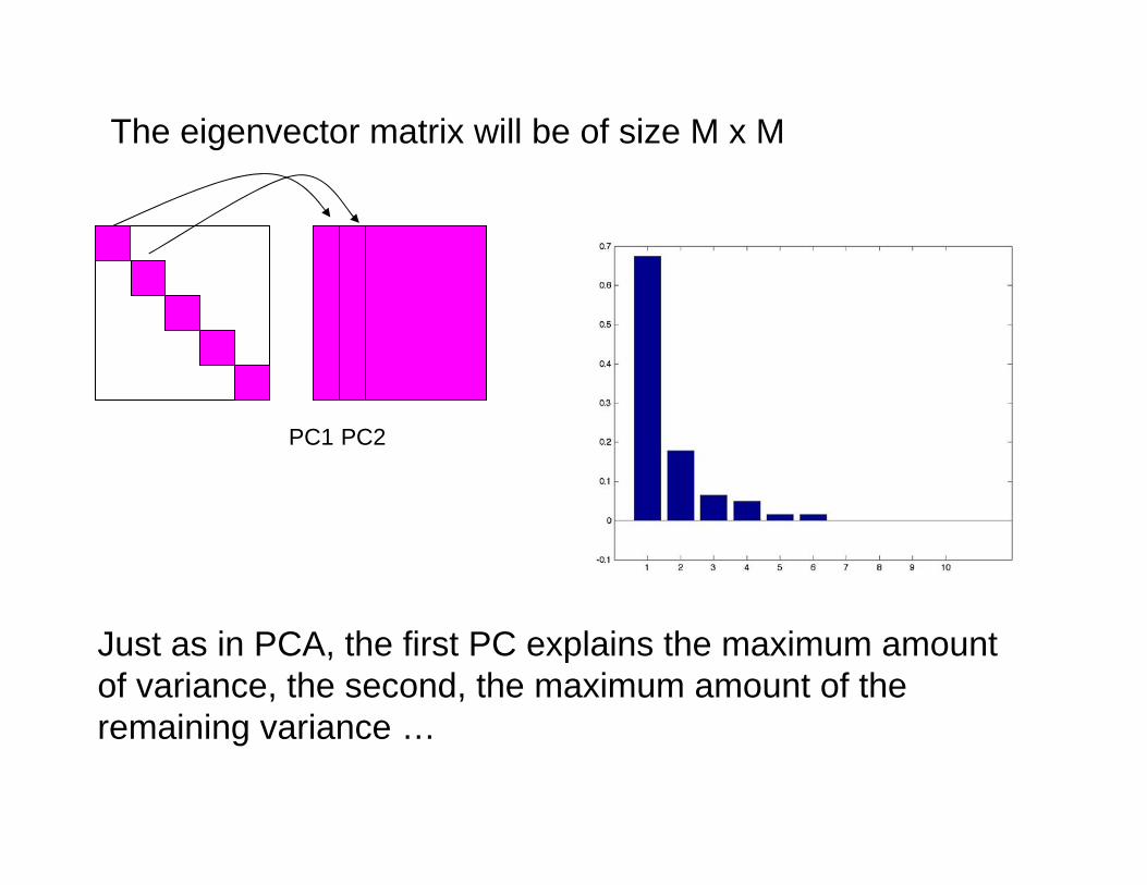
The eigenvector matrix will be of size M x M

Just as in PCA, the first PC explains the maximum amount of variance, the second, the maximum amount of the remaining variance …

PC1 PC2

Notice that the eigenvectors that are clearly oscillatory come in pairs that represent the same frequency.

To visualize the data, we scale the eigenvector by the ampitude that it represents.

E Λ1/2

We define the PCs, just as in PCA:PC = ETX

X = E PC

M

M

K

M (P

C)

KM (P

C)

=

M

K M (PC)

M

KM

(PC

)

=

“Y contains the principal component scores, the amplitudes by which you multiply the eigenvectors to get the original data back.”

X = E PCM

K M (PC)

M

K

M (P

C)

=

“Y contains the principal component scores, the amplitudes by which you multiply the eigenvectors to get the original data back.”

But this step is a bit tricky because remember that you want to reconstruct your original timeseries, but the one in X is truncated.

=

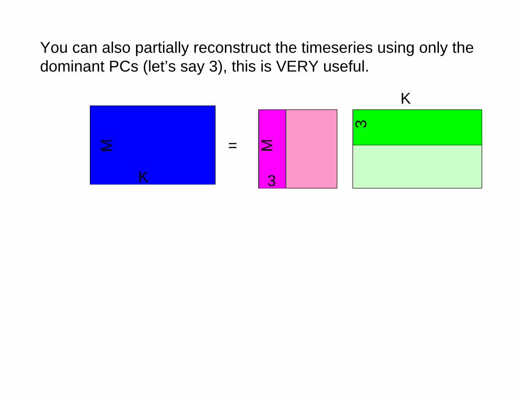
You can also partially reconstruct the timeseries using only the dominant PCs (let’s say 3), this is VERY useful.

M

K

M

K

3

3

for i=1:183U(i) = 10*sin(2*pi()*i/150)+2*cos(2*pi()*i/5)+ 4*cos(2*pi()*i/20);

end

% First, let's remove the meanT = U - mean(U);

% The maximum lag will be 40 days% Construct trayectory matrixM = 40;N = 183;K = N-M+1;

for l=1:40X(l,:) = T(l:N-M+l);

end

% Calculate the covariance matrixC = (1/(K-1)) * X * X';

% Perform Eigenanalysis[VEC,VAL] = eig(C);

% Check variances and calculate the traceVarTOT = trace(VAL);check = trace(C);

% Look at the variances for first 10 PCsVar = diag(real(VAL));RelVar = real(Var)/VarTOT;figure(1)bar(RelVar(1:10))saveas(gcf,'RelativeVar.jpg')

% Look at the eigenvectorsfigure(2)for i=1:6

vecplot = VEC(:,i)*VAL(i,i)^0.5subplot(4,2,i), plot(vecplot)endsaveas(gcf,'eigenvectors.jpg')

% Calculate the PCsPC = VEC' * X;

%Calculate reconstructed componentsRC = zeros(N,K);for k = 1:M

kfor i = 1:M-1

xi = 0.;for j = 1:i

xi=xi + PC(k,i-j+1)*VEC(j,k);endRC(i,k) = xi/i;

endfor i = M:K

xi = 0.;for j = 1:M

xi=xi + PC(k,i-j+1)*VEC(j,k);end;RC(i,k) = xi/M;

endfor i = K+1:N

xi = 0.;for j = i-N+M:M

xi=xi + PC(k,i-j+1)*VEC(j,k);end;RC(i,k) = xi/(N-i+1);

endend

figure(3)for i=1:6

RCtot = sum(RC(:,1:i),2);subplot(4,2,i), plot(RCtot)

endsubplot(4,2,8), plot(T,'g')saveas(gcf,'Reconstruction.jpg')

http://www.atmos.ucla.edu/tcd/ssa/

M-SSA is the multivariate extension to SSA. You are essentially extracting common trends and oscillatory patterns from a group of variables.

Mathematically it is very similar to SSA, now you have L variables (in this case L=2).

M-SSA

T1 T2 … TKT2 T3 … TK+1

TM TK+1 … TNM

* L rows (w

indow length)

K columns (K=N-M+1)

X =

M*L

K

S1 S2 … SKS2 S3 … SK+1

SM SK+1 … SN

If you are dealing with different variables (say winds and precipitation) you must normalize the data before doing any analysis. That way you are comparing apples to apples.

L*M

L*M

The covariance matrix now has dimensions L*M x L*M, and it represents the autocovariance and cross-covariance terms

C =

T T T S

S T S S

We perform eigenanalysis on the covariance matrix. You now have L*M eigenvectors and eigenvalues

T

=

Λ = ET C E = λ1

λ2

λL*M

The set of eigenvectors eiand eigenvalues λi represent a coordinate transformation where C becomes a diagonal.

L*ML*M

L*M

The PCs will have dimensions L*M x K

PC = ETX

L*M

L*M

K

L*M

(PC

)

K

L*M

(PC

)

=

The reconstruction is essentially the same, except that the messy loop will have an outer “if” statement representing the variable (loop not shown).

X = E PC

L*M

L*M

K L*M (PC) K

L*M

(PC

)

=

Application of SSA and M-SSA to land-atmosphere Interactions

Precipitation recycling is the contribution of local evapotranspiration to precipitation events.

The time series of r indicates the daily fraction of precipitation that came from evaporative origin.

Region 8.2

Central USA Plains

0

0.1

0.2

0.3

4/1/85 5/1/85 5/31/85 6/30/85 7/30/85 8/29/85 9/28/85

Recycling Ratio (r)

Our objective is to understand what causes the spatio-temporal variability of precipitation recycling.

⎥⎦

⎤⎢⎣

⎡−−= ∫

τ

τωε

0

'exp1 dR

Ratio of Evaporation over total precipitablewater. E/w

Depends on the size of the region and the velocity of the winds.

Inherent to the model

Precipitation

Temperature

Sensible Heat Flux

Atmospheric Humidity

Not explicitly included in model formulation

We begin with SSA:

• You can use EOF analysis to look at the structure of a timeseries by doing and eigenanalysis of the lagged covariance matrix. (Ghil et al. 2002)

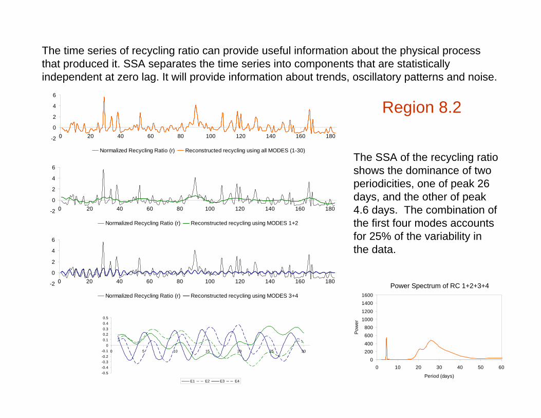
The time series of recycling ratio can provide useful information about the physical process that produced it. SSA separates the time series into components that are statistically independent at zero lag. It will provide information about trends, oscillatory patterns and noise.

-2

0

2

4

6

0 20 40 60 80 100 120 140 160 180

Normalized Recycling Ratio (r) Reconstructed recycling using all MODES (1-30)

-2

0

2

4

6

0 20 40 60 80 100 120 140 160 180

Normalized Recycling Ratio (r) Reconstructed recycling using MODES 1+2

-2

0

2

4

6

0 20 40 60 80 100 120 140 160 180

Normalized Recycling Ratio (r) Reconstructed recycling using MODES 3+4

-0.5-0.4-0.3-0.2-0.1

00.10.20.30.40.5

0 5 10 15 20 25 30

E1 E2 E3 E4

The SSA of the recycling ratio shows the dominance of two periodicities, one of peak 26 days, and the other of peak 4.6 days. The combination of the first four modes accounts for 25% of the variability in the data.

0200400

600800

10001200

14001600

0 10 20 30 40 50 60

Period (days)

Pow

er

Power Spectrum of RC 1+2+3+4

Region 8.2

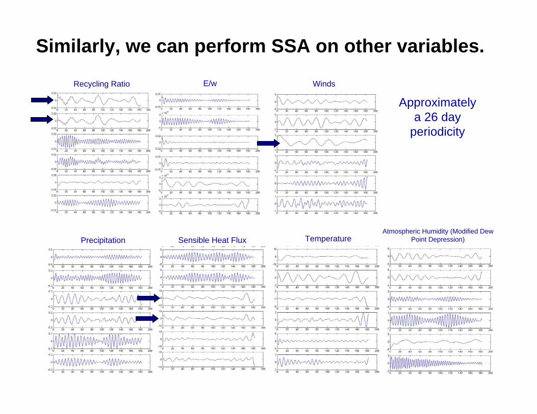
Similarly, we can perform SSA on other variables.

Recycling Ratio E/w Winds

Precipitation Sensible Heat Flux TemperatureAtmospheric Humidity (Modified Dew

Point Depression)

Approximately a 26 day

periodicity

-2-10123

0 20 40 60 80 100 120 140 160 180-0.040

-0.020

0.000

0.020

0.040

RC WIND MODE 4" RC r MODES 2+3"

-15-10

-505

1015

0 20 40 60 80 100 120 140 160 180

-0.040

-0.020

0.000

0.020

0.040

RC SHTFL MODE 4+5" RC r MODES 2+3"

Looking only at the twenty six day periodicity. Recycling is out of phase with the winds, and in phase with the sensible heat flux.

Similarly, we can perform SSA on other variables.Recycling Ratio E/w Winds

Precipitation Sensible Heat Flux TemperatureAtmospheric Humidity (Modified Dew

Point Depression)

Approximately a 5 day

periodicity

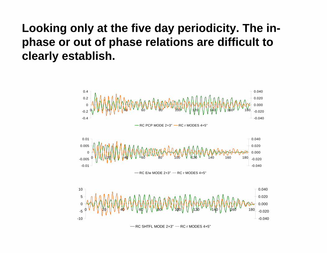
Looking only at the five day periodicity. The in-phase or out of phase relations are difficult to clearly establish.

-0.01

-0.005

0

0.005

0.01

0 20 40 60 80 100 120 140 160 180

-0.040

-0.020

0.000

0.020

0.040

RC E/w MODE 2+3" RC r MODES 4+5"

-0.4

-0.2

0

0.2

0.4

0 20 40 60 80 100 120 140 160 180

-0.040

-0.020

0.000

0.020

0.040

RC PCP MODE 2+3" RC r MODES 4+5"

-10

-5

0

5

10

0 20 40 60 80 100 120 140 160 180

-0.040

-0.020

0.000

0.020

0.040

RC SHTFL MODE 2+3" RC r MODES 4+5"

We need a methodology to account for the different timescales in land-atmosphere processes.

RR SMPP

Midwestern United States

We need a different methodology if we want to find relations among variables. Multivariate singular spectrum analysis (M-SSA) enables us to go the extra step.

Multivariate Singular Spectrum Analysis allows us to account for the different timescales of the system.

RR

SH RR

PP

EVP

SM

18 Variables


RR

0

0.1

0.2

0.3

30-Mar 19-May 8-Jul 27-Aug 16-Oct

The purpose of M-SSA is to maximize the joint variance of all the variables.

In a way that accounts for both their autocorrelation and the correlation between different variables.


SH

0

40

80

30-Mar 19-May 8-Jul 27-Aug 16-Oct

RR

RR1 RR2

RRK

…

RR2 RR3

RRK+1

…

SH1 SH2

SHK

SH2 SH3

SHK+1

SHM RRM+1

SHK+M

… … ……RRM RRM+1

RRK+M

……

PP

EVP

SM

X =

…..

…..

…..

C = XTXLagged autocorrelation and cross correlation matrix

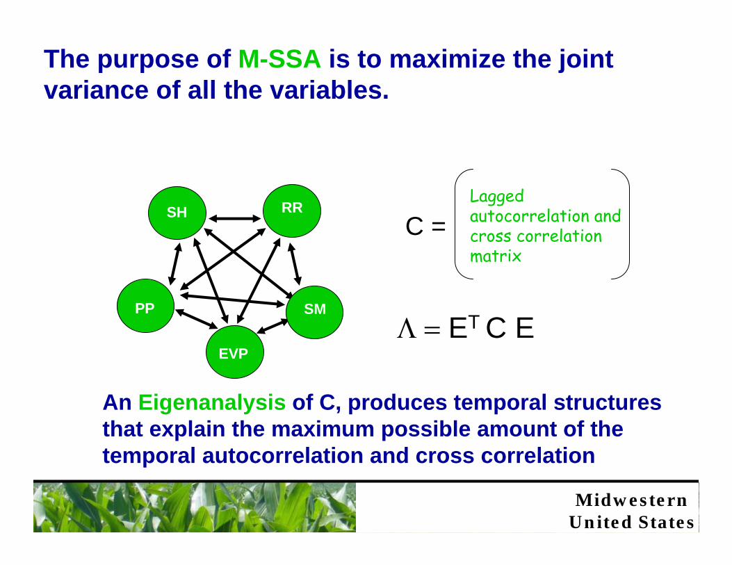
The purpose of M-SSA is to maximize the joint variance of all the variables.

C =

Λ = ET C E

An Eigenanalysis of C, produces temporal structures that explain the maximum possible amount of the temporal autocorrelation and cross correlation

Lagged autocorrelation and cross correlation matrix


RRSH

RR

PP

EVP

SM

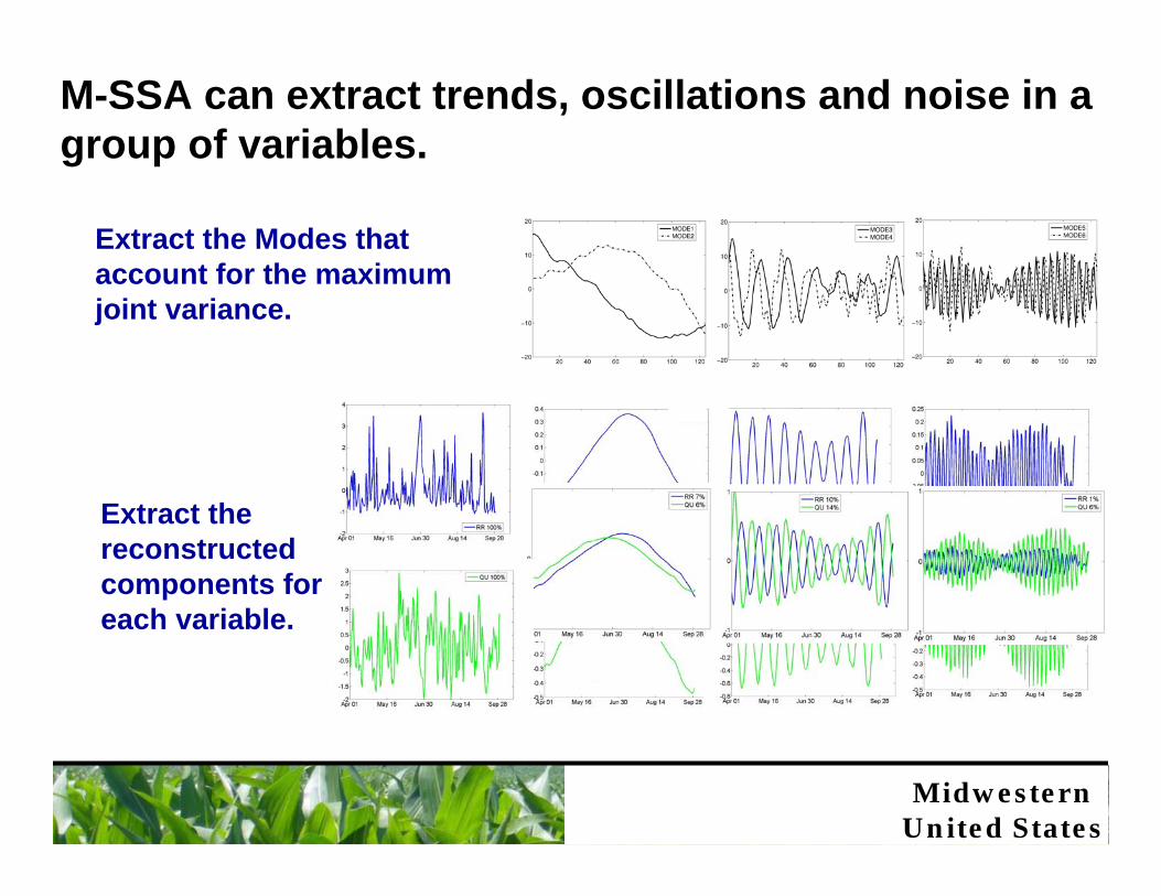
M-SSA can extract trends, oscillations and noise in a group of variables.

Extract the Modes that account for the maximum joint variance.

Extract the reconstructed components for each variable.



0

10

20

30

40

1985 1986 1987 1988 1989 1990 1991 1992 1993 1994 1995P

erio

dici

ty (d

ays)

For each of the 11 years we extract the two dominant oscillatory components.

1988 (drought) has the longest periodicities and 1993 (flood) has the shortest.

Component 1

Component 2

To understand what these modes look like in the “real world” we can visualize the representative days.

Year 1994 Modes 7+8

0

0.2

Composite of High recycling days

0

0.2

Composite of Low recycling days


-1

-0.5

0

0.5

1RR PP

May 20 Jul 9 Aug 28

At short timescales the recycling ratio is enhanced when precipitation and precipitable water are low.

RR

& P

reci

pita

ble

Wat

erR

R &

Pre

cipi

tatio

nCorr = -0.55

Phs Diff = 136.37º

Corr = -0.74

Phs Diff = 148.55º

1994

Precipitation during:

Days of high recycling.

Days of low recycling

Precipitable Water during:




At short timescales the recycling ratio is enhanced when precipitation and precipitable water are low.

Reason: Recycling only becomes important when advectedprecipitation decreases.

The moisture for intense summer storms is mainly of advective origin.


At short timescales the recycling ratio is enhanced when winds and moisture fluxes are low.

RR

& M

erid

. Moi

stur

e Fl

uxR

R &

Zon

al M

oist

ure

Flux Corr = -0.71

Phs Diff = 139.85º

Corr = -0.7

Phs Diff = 147.23º

1994Zonal Moisture Flux during:



Meridional Moisture Flux during:




At short timescales the recycling ratio is enhanced when winds and moisture fluxes are low.

Reason:

The air has more time to traverse the region and pick up evapotranspiredmoisture.


1994

At short timescales the recycling ratio is enhanced when sensible heat and cloud base height are high.

Zonal Moisture Flux during:



Meridional Moisture Flux during:



RR

& C

loud

Bas

e H

eigh

tR

R &

Sen

sibl

e H

eat

Corr = 0.71

Phs Diff = 31.23º

Corr = 0.5

Phs Diff = 46.49º


Why? Because the dry soil will have a much faster growth of the boundary layer.

In some cases, the atmosphere over dry soil (high sensible heat) will reach the level of free convection before the moist soil.

LFC

Less Humid

More Humid

Reason: Sensible heat flux increases BL depth and promotes convective cloud formation.


High Sensible Heat Low Sensible Heat

Contrary to what one might expect, at timescales < 40 days evapotranspiration variability is NOT related to recycling variability .

In non-drought years : In this moisture abundant region, soil moisture anomalies will not stress vegetation

Evapotranspi-ration will not be affected.

Recycling will not be affected.


At long timescales (>40 days), the recycling ratio is related to evapotranspiration only during dry years.

1988 drought year

1986 normal year

1993 flood year

This result is quite surprising!Midwestern

United States

Precipitation decreases

Soil Moisture decreases

Evaporation decreases

Transpiration continues

Sensible Heat

increases

Contributes to Atmos. moisture

Boundary Layer grows

Promotes Convective Cloud

Formation

Is θe large enough for convection?

Wat

er

Cyc

le

Energy

Cycle

Is there root-accessible

soil moisture?

yes

yes

Less Contribution to Atmos. Moisture

no

Entrainment of low θe air

Suppressed Cloud Formation

no

Temperature increases

Promotes Precipitation

In the Midwest precipitation recycling acts as a mechanism for ecoclimatologicalstability through local negative feedbacks.


geophysical applications of singular spectrum analysis ... · pdf filegeophysical applications...

Documents