Multi-Objective Optimization of a Tube Bundle Heat Exchanger

Vanja Skuric1, Tessa Uroic1, Henrik Rusche2

1 Faculty of Mechanical Engineering and Naval Architecture, Zagreb, Croatia 2 Wikki GmbH, Braunschweig, Germany

9th OpenFOAM Workshop

23-26 June 2014 in Zagreb, Croatia

p. 1

Content • Geometry optimization

• Heat exchanger problem

• Workflow

• Software

• Case setup

• Results

• Work in progress and in the future

p. 2

Geometry Optimization

Heat exchanger max(ΔT) and min(Δp)

Tube position optimization

Airfoil max(CL) and min(CD)

Shape optimization

p. 3

Heat Exchanger Problem • Objective:

– Find optimal tube positions for maximum temperature increase and minimum pressure drop

• Parameters: – Tube positions ─ coordinates ( x1 ... x4 , y1 ... y4 )

• Objective Functions: – Pressure drop, Δp – Temperature increase, ΔT

• Constraints: – Tubes cannot be in contact (two different approaches):

• restricting x position (x-corridor) • nonlinear distance constraints

• 2D case

p. 4

Workflow

Optimization software (algorithm)

Geometry generator (CAD)

CAD file

Mesh generation utility

CFD software package

Optimization workflow

Mesh

( x1 ... x4 , y1 ... y4 )

Δp, ΔT

p. 5

Software • Dakota (Sandia National Laboratories)

– A Multilevel Parallel Object-Oriented Framework for: • Design Optimization • Parameter Estimation • Uncertainty Quantification • Sensitivity Analysis

– Here: Evolutionary Algorithm (derivative-free global algorithm)

• Salome (EDF, CEA, OpenCascade) – CAD and Post-Processing – Graphical user and terminal user interface – Here: TUI with python script for cylinder geometry generation

• OpenFOAM – Meshing (blockMesh and snappyHexMesh) – Solver (buoyantBoussinesqSimpleFoam) – Post-processing (swak4Foam): Average pressure drop and temperature increase

from inlet to outlet

p. 6

Software

Optimization software (algorithm)

Geometry generator (CAD)

STL file

Mesh generation utility

CFD software package

Optimization workflow

Mesh

( x1 ... x4 , y1 ... y4 )

Δp, ΔT

Dakota (EA algorithm)

Salome (python script)

OpenFOAM (meshing)

OpenFOAM (solver)

p. 7

Case setup - Dakota • Method:

– Multi-objective genetic algorithm MOGA (JEGA library) • Population sizes: 40, 60, 80 • Number of generations: 5, 10 ,15, 20 • Crossover type – shuffle random

– number of parents = population size – number of children = 75% of population

• Mutation type – offset normal – mutation rate = 100% – mutation scale = 10%

• Replacement type – elitist

• Variables: – 8 variables ( x1 ... x4 , y1 ... y4 ) – Constraints (two approaches):

• 6 x-corridors: inlet corridor, 4 tube corridors, outlet corridot • 3 x-corridors: inlet corridor, tube corridor, outlet corridor – minimal tube distance as a constraint

• Response functions: – 6 x-corridors – 2 response functions: Δp, ΔT – 3 x-corridors – 8 response functions: Δp, ΔT, 6 distance values between cylinders

p. 8

Case setup - Dakota • 6 x-corridors

• 3 x-corridors

p. 9

Case setup - OpenFOAM • Fluid - Air • Boundary conditions:

– Inlet – velocity inlet • U = (0.01 0 0) m/s • T = 293 K • Re = 14 (laminar flow, steady state)

– Top and bottom – cyclicAMI – Cylinders - wall

• constant temperature, T = 353 K

– Outflow • p = 0 Pa (gauge pressure)

• Post-processing (swak4Foam) – Δpavg and ΔTavg

p. 10

Results

p. 11

0,14

0,16

0,18

0,2

0,22

0,24

0,26

0,28

0,3

0,32

0,34

0,36

0,38

25 27 29 31 33 35 37 39 41 43 45

Δp [

mPa

]

ΔT [K]

10 gen (40 pop)

Results • The result of the bi-objective optimization is the Pareto-front – the line of optimal

solutions.

p. 12

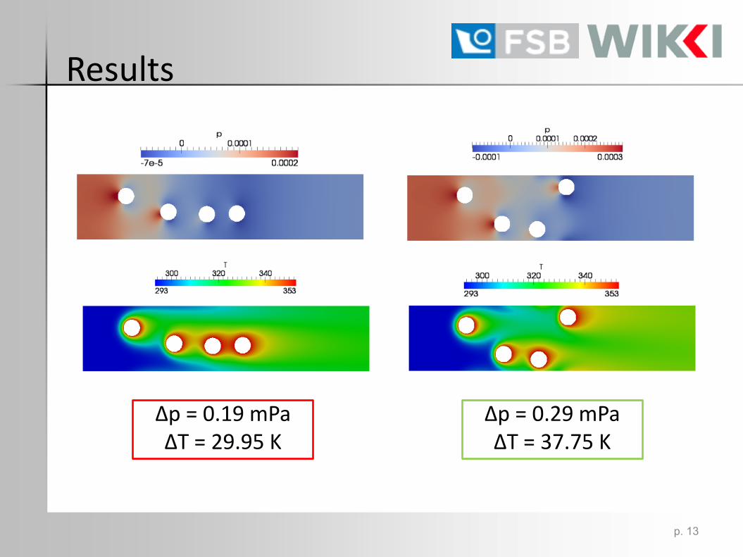
Results

Δp = 0.19 mPa ΔT = 29.95 K

Δp = 0.29 mPa ΔT = 37.75 K

p. 13

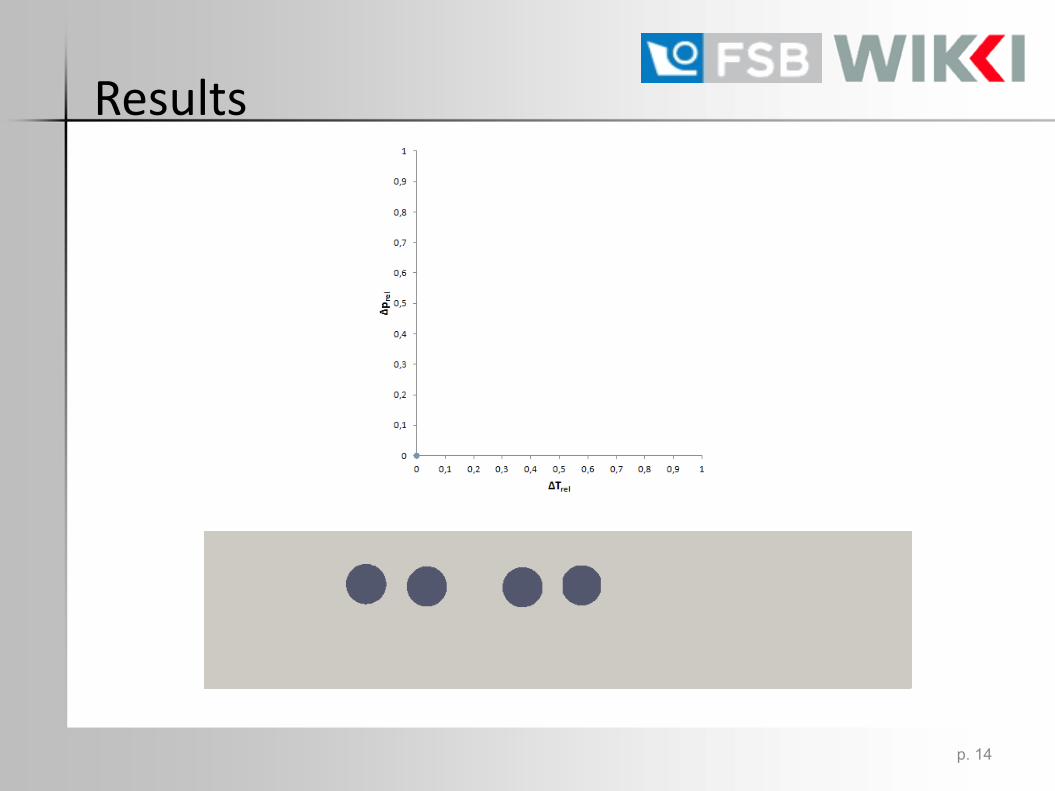
Results

p. 14

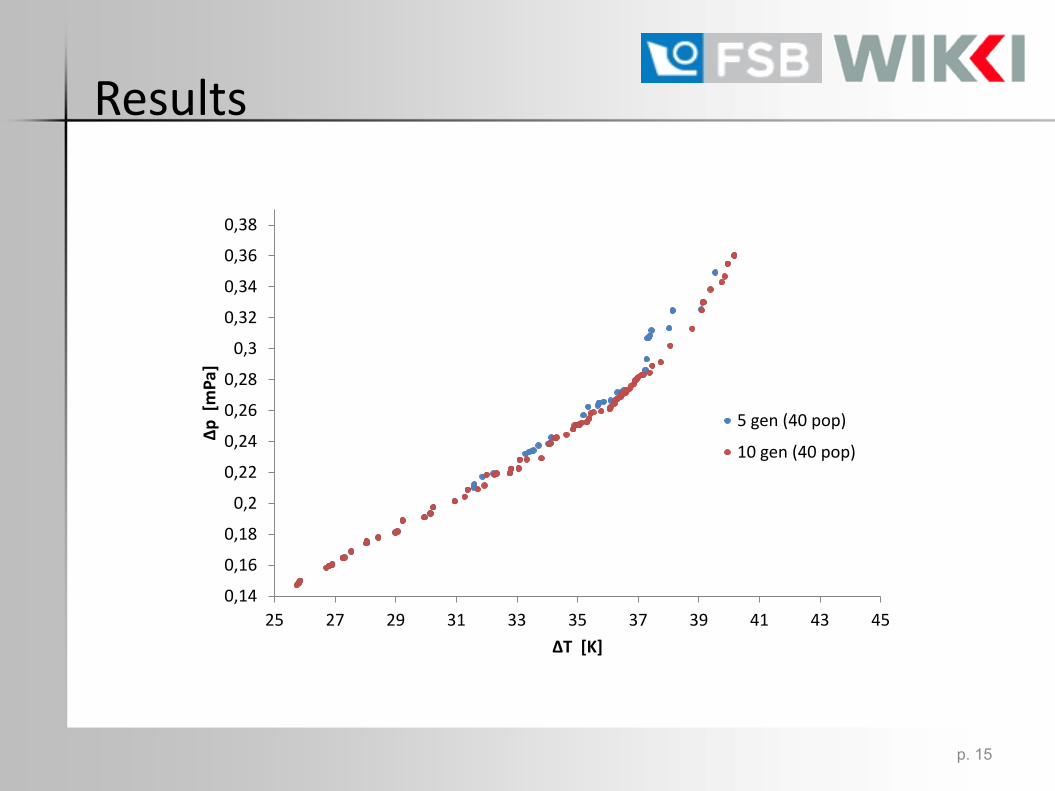
Results

0,14

0,16

0,18

0,2

0,22

0,24

0,26

0,28

0,3

0,32

0,34

0,36

0,38

25 27 29 31 33 35 37 39 41 43 45

Δp [

mPa

]

ΔT [K]

5 gen (40 pop)

10 gen (40 pop)

p. 15

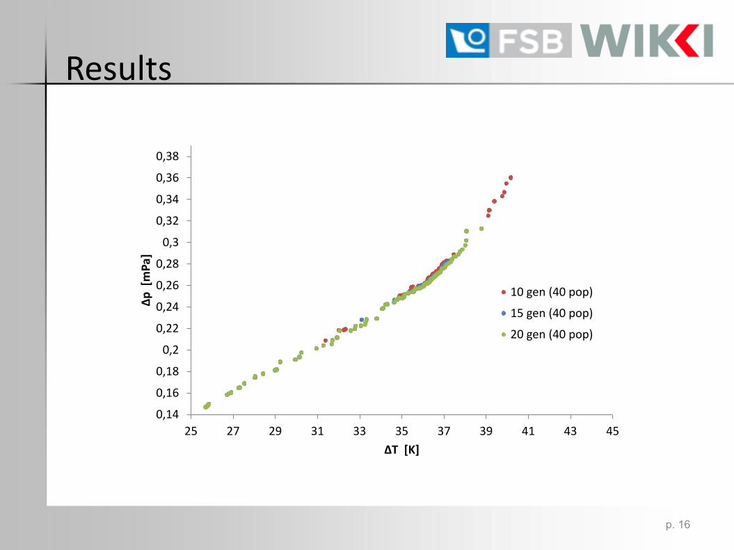
Results

0,14

0,16

0,18

0,2

0,22

0,24

0,26

0,28

0,3

0,32

0,34

0,36

0,38

25 27 29 31 33 35 37 39 41 43 45

Δp [

mPa

]

ΔT [K]

10 gen (40 pop)

15 gen (40 pop)

20 gen (40 pop)

p. 16

Results

0,14

0,19

0,24

0,29

0,34

0,39

0,44

0,49

0,54

0,59

0,64

25 27 29 31 33 35 37 39 41 43 45

Δp [

mPa

]

ΔT [K]

20 gen (40 pop)

20 gen (40 pop) 3 x-corr.

p. 17

Results

0,14

0,19

0,24

0,29

0,34

0,39

0,44

0,49

0,54

0,59

0,64

25 27 29 31 33 35 37 39 41 43 45

Δp [

mPa

]

ΔT [K]

20 gen (40 pop) 3 x-corr. 10 gen (80 pop) 3 x-corr.

p. 18

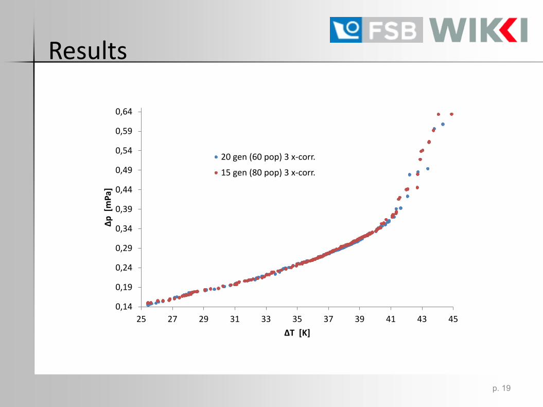
Results

0,14

0,19

0,24

0,29

0,34

0,39

0,44

0,49

0,54

0,59

0,64

25 27 29 31 33 35 37 39 41 43 45

Δp [

mPa

]

ΔT [K]

20 gen (60 pop) 3 x-corr.

15 gen (80 pop) 3 x-corr.

p. 19

Results

0,14

0,19

0,24

0,29

0,34

0,39

0,44

0,49

0,54

0,59

0,64

25 27 29 31 33 35 37 39 41 43 45

Δp [

mPa

]

ΔT [K]

5 gen (80 pop) 3 x-corr.

10 gen (80 pop) 3 x-corr.

15 gen (80 pop) 3 x-corr.

p. 20

Work in progress and in the future

In progress: – Uncertainty quantification – Robustness evaluation of the optimal points

In the future: – Workflow for obtaining pareto front using the

single objective algorithms – Optimization with gradient based methods

p. 21

Thank you!

p. 22