multi-objective optimal scheduling of a hybrid ferry with
TRANSCRIPT
electronics
Article
Multi-Objective Optimal Scheduling of a HybridFerry with Shore-to-Ship Power Supply ConsideringEnergy Storage Degradation
Kyaw Hein 1,* , Xu Yan 1,* and Gary Wilson 2
1 School of Electrical and Electronic Engineering, Nanyang Technological University,Singapore 639798, Singapore
2 Rolls-Royce Electrical, Rolls-Royce, Singapore 639798, Singapore; [email protected]* Correspondence: [email protected] (K.H.); [email protected] (X.Y.)
Received: 29 April 2020; Accepted: 19 May 2020; Published: 20 May 2020�����������������
Abstract: To improve the operation efficiency and reduce the emission of a solar power integratedhybrid ferry with shore-to-ship (S2S) power supply, a two-stage multi-objective optimal operationscheduling method is proposed. It aims to optimize the two conflicting objectives, operation cost(fuel cost of diesel generators (DGs), carbon dioxide (CO2) emission tax and S2S power exchange)and energy storage (ES/ESS) degradation cost, based on the preference of the vessel operator andsolar photovoltaic (PV) power output. For the day-ahead optimization, interval forecast data ofthe PV is used to map the solution space of the objectives with different sets of weight assignment.The solution space from the day-ahead optimization is used as a guide to determine the operatingpoint of the hour-ahead optimization. As for the hour-ahead scheduling, more accurate short-leadtime forecast data is used for the optimal operation scheduling. A detailed case study is carried outand the result indicates the operation flexibility improvement of the hybrid vessel. The case studyalso provides more in-depth information on the dispatching scheme and it is especially important ifthere are conflicting objectives in the optimization model.
Keywords: energy storage; electric ship charging; generation scheduling; hybrid electric ferry;multi-objective optimization; operation scheduling; renewable energy sources; shore-to-ship power
1. Introduction
In 2008, more than 90% of global trading was carried out by maritime transportation and itis expected to be tripled by 2025. The international maritime organization (IMO) stated that if nonecessary actions are taken to improve the energy efficiency of the vessel, carbon dioxide (CO2)emission will increase by 250% by the end of 2050 [1]. Emission at the harbor area has greaterinfluences on the onshore environment and hence the operation of vessels near shore becomes themajor concern for the marine industry [2–4]. The emission level of the ships is restricted by theauthorities and some of the on-board diesel generators (DGs) are forced to switch off when the vesselis approaching the harbor. Improvement measures such as renewable energy source (RES), energystorage system (ESS) and shore-to-ship (S2S) power supply integration, are proposed by regulatoryauthorities, and many literatures [5–26] have pointed out the applicability of such technologies onship power system operation. The proposed technologies introduce additional flexibility, as well ascomplexity in the system operation scheduling, and hence should be thoroughly explored. As a result,the key research challenge is to design an optimal operation scheduling of the more-electric vesselwith the consideration of the proposed improvement measures.
Electronics 2020, 9, 849; doi:10.3390/electronics9050849 www.mdpi.com/journal/electronics
Electronics 2020, 9, 849 2 of 21
2. Literature Review
In [5], the initiatives toward sustainable transport systems with the help of RESs such as PV arehighlighted. The findings indicate that RESs can significantly reduce the overall fuel consumption ofthe transportation network if they are managed efficiently. However, RESs are stochastic in natureand the addition of such energy sources adds complexity to the system optimal operation scheduling.The uncertainty presents in PV power generation can be efficiently addressed by the integration ofthe ES. ES not only addresses the uncertainty present in the RESs [5,6] but also provides additionaldimensions to the optimal operation scheduling of the vessels such as optimal loading of the DGs, peakshaving, energy reserve, and uninterruptible power supply [11,13,14,17–20]. Yet, full battery-poweredvessels are still fewer in number due to the limited capacity of the ES for longer voyages. Only ashort duration battery-powered or hybrid vessels are tested and developed much more frequently.An extensive simulation study in [21] has demonstrated that ES can reduce the fuel consumption ofmore-electric ships. The multi-objective nature of the ship power system with ES is further analyzedin [14]. The study has considered cooperating objectives such as fuel consumption minimizationand emission reduction. The result indicates that aside from the fuel consumption reduction, ES canalso reduce the overall CO2 emission per transport work. However, such a form of the objectiveformulation will result in ES to be charged and discharged much more frequently and hence resultingin the accelerated degradation of the ES. Furthermore, the effects of ESS integration on the PV integratedvessels are also analyzed in [15,16,23], and the results indicate that proper deployment of the ES cansuccessfully address the uncertainty present in the PV uncertainty while reducing the overall emissionof the vessel. Generally, the S2S power supply system or cold-ironing is used to further curtail theemission at seaport territory while assisting the charging of the ES. The S2S power supply allowssome or all the on-board DGs to be switched off while the vessel is at berth. A hybrid DGs/ES vesselcan benefit greatly from the S2S power supply [5,6,11]. However, the S2S power supply might usenon-renewable resources, and hence economic factors are needed to be considered while designing theoperation scheduling of the ship power system for the grid-connected operation mode [12].
In [13,14,17–19], the energy management strategies for the hybrid vessels are presented. Most ofthem address the emission and fuel cost minimization as their main objective in the optimizationproblem. However, these two objectives encourage the heavy reliance on the ES and the renewablepower generation. Over-reliance on the ES will result in frequent charging, discharging, and a highramp rate that can cause accelerated degradation. In literature, the impact of the operation loadprofile on the ES degradation is highlighted in [7,8] for the land-based power system. In [9], a generalapproach based on the forecast and the receding horizon is proposed for optimal operation whileaccounting for degradation reduction of the ES. Two-layer energy management of the microgrid withenergy storage degradation cost is presented in [10]. However, these literatures mainly focus on theland-based power system and the optimal operation of the ES for the marine power system are yet tobe explored. Furthermore, the operation of the ship power system is different from the land-basedpower system in the following ways, (1) fixed schedule for the grid-connected (at the harbor) andislanded mode of operation (during transit) (2) have higher ES to power system ratio (3) influenced bythe propulsion requirements and port arrival time. These have to be accounted for in the modelingand design of the optimal scheduling of the ship.
As for the existing work in the literature for the optimal operation scheduling of ship powersystems, a dynamic programming approach is used to limit greenhouse gas emissions with the help ofES in [21]. Rule-based and Grey wolf optimization methods are compared in [22] for fuel consumptionminimization and emission reduction for the electric ferries. Interval optimization of the hybrid vesselwith solar PV integration for the oil tanker is presented in [23]. It aims to minimize the fuel andemission cost while considering the investment cost of the ES. Generation and voyage schedulingwith the demand-side response are presented in [14,17,24] which minimize fuel consumption byappropriately adjusting the propulsion speed of the vessel. The result proves that the optimal voyagescheduling will tend to benefit large vessels which have significant impact on the drag and hull
Electronics 2020, 9, 849 3 of 21
resistance coefficients with the adjustment in the propulsion speed. Despite the attempts to reduce thefuel consumption and emission, the operation scheduling of the ship power system is multi-objective innature and the conflicting objectives of the system operation scheduling have to be carefully addressed.The vessel operators aim to optimize the operation cost (fuel consumption, cost of charging from theS2S power supply and maintenance cost), emission cost/carbon tax and ES degradation cost based onthe operating scenarios. A single objective optimization approach will tend to result in over-relianceon the resources which are not considered in the objective function. In fact, there are not many studieson the optimal operation scheduling of ship power systems which consider all the aforementionedfactors. Even if the multi-objective optimization methods are proposed, the performance analysis ofthe dispatch result of the multi-objective optimization is yet to be investigated. Furthermore, the effectof grid electricity price on the operation of hybrid vessels is not fully investigated. Thus, this paperinvestigates the optimal operation scheduling of the hybrid vessels that consider the grid electricityprice of S2S power supply, renewable energy sources, ES degradation, and greenhouse gas emissionwith the help of multi-objective optimization.
To have a better understanding of the current state of the art for the ship power system operationscheduling, two recent studies with similar research direction with the proposed method in this studyare identified. The selected research works on the optimal operation scheduling of the ship powersystem are illustrated in [25,26]. To highlight the key differences from the proposed approach inthis study, comparison with the above references are illustrated. In [25], multi-objective operationscheduling of the ship power system is carried out with a meta-heuristic optimization approach byconsidering the operation cost and emission of the vessel. Similar work on the operation scheduling ofa cruise vessel is also presented in [26] with very similar modeling and method as illustrated in [25].It employs a multi-objective deterministic optimization to identify the optimal operating point of acruise vessel. However, the aforementioned studies have yet to consider the potential integration ofsolar PV on-board the ship power system and how the solar irradiation variation will influence the finaldispatch parameters of the multi-objective optimization of the vessel. For the proposed approach inthis research work, the weight assignments of the multi-objective functions are carefully addressed byaccounting the day-ahead prediction interval data of solar irradiation. A two-stage dispatch approachwith different optimization time resolutions is also proposed to improve the dispatch accuracy andreliability of the vessel. The proposed approach also highlights and demonstrates that the selectionof the optimal operating points for the hour-ahead operation from the Pareto solution front is not atrivial task from the vessel operator’s point of view. Thus, detailed analysis such as the average rate ofchange of SOC and the Pareto front shifting with changes in the weight assignment and stochasticvariable such as solar irradiation is required to be analyzed to provide a better understanding of theoptimal operating point of the vessel. Such analyses are yet to be thoroughly explored and presentedin the literature. Furthermore, the research works in [25,26] have yet to consider the impact of ESdegradation in the multi-objective model. Generally, in the ship power system, ES is integrated notonly to ensure the emission improvement but also to improve the generation dispatch reliability byacting as a spinning reserve, emergency energy reserve, or in the standby mode of operation. As aresult of the high investment cost, the use of ES should be carefully designed and incorporated into theobjective formulation. As the degradation of the ES is not considered in the above studies, the depth ofdischarge (DOD) of the ES is higher and hence significantly affects the life of the ES. The energy reserveof ES for the emergency mode of operation is also not adhered to in these studies. In this research work,the dispatch reliability is addressed by allowing the vessel operators to identify how the ES should beoperated based on the solar PV generation. The energy reserve from the ES can be set by selecting anappropriate operating point from the Pareto front solution space. The weight assignment will alsoaffect the ramp rate of the ES and hence vessel operators have more control over the way the vesselshould be operated. Furthermore, these studies have yet to model the integration of S2S and how thegrid electricity price will influence the energy exchange with the main grid. Moreover, the above studyfocuses on the multi-energy system which is only applicable to vessels with high thermal load demand
Electronics 2020, 9, 849 4 of 21
such as cruise ships. However, in this study, a more-electric vessel with a higher penetration of the ESand solar PV are addressed to cover the wider types of vessel in the marine industry. The detailedcontributions of this research work are further summarized in the following section.
3. Contributions
The main contributions of this paper are summarized: (1) A two-stage multi-objective optimizationproblem is modeled for a hybrid vessel that encompasses the operation, emission, and ES degradationcost. The first stage (day-ahead) optimization attempts to map the solution space based on thePV interval prediction data for the performance comparison of the objective functions. From this,the optimal weights selection based on the user’s preference is selected for the second stage(hour-ahead) with shorter-time and more accurate prediction data. It allows the vessel operatorswith a basic understanding of optimization to understand the differences in the dispatch strategywith the changes in the solar irradiation (2) Analytical model of the ES degradation is modeled toincorporate into the optimal scheduling of the ship power system. Static and dynamic degradationof ES are considered for optimal scheduling which are ignored in other literature. (3) The demandresponse electricity pricing of the S2S power supply is modeled to illustrate the accurate representationof the system which has grid charging or S2S capability. (4) The impact of the uncertainty nature ofthe PV on the weight assignment is addressed with two stages of optimization before and after theuncertainty realization. Case studies with a hybrid ferry are illustrated to demonstrate the proposedoptimal scheduling. Hybrid ferry with shorter voyage distance and enough berthing duration isillustrated as a case study due to its potential benefit from the PV, ES, and S2S integration. However,there is a generality in the proposed approach and can be applied to any other type of vessel.
4. Proposed Optimal Dispatch Scheme of Hybrid Ferry with Shore-to-Ship Power Supply
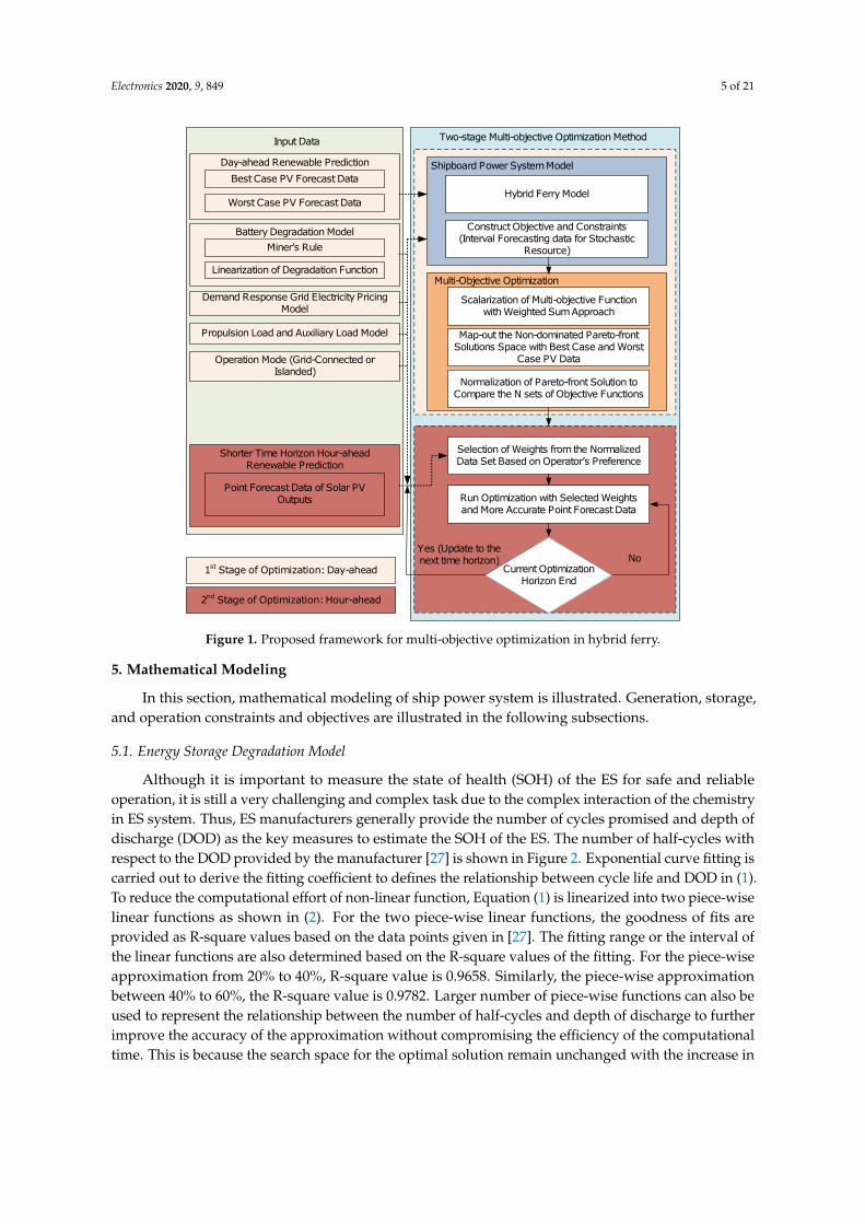
The proposed optimal dispatch scheme of a hybrid ferry involves two stages of multi-objectiveoptimizations. The main aim of the first stage of optimization is to map-out the Pareto front solutionspace based on the interval forecast data of the solar PV output and compare the performancesof the different solution sets with the help of normalization. Mapping of the solution space is atime-consuming process and the optimal weights selection for the objective functions requires adetailed understanding of the performance of the model at different operating points in the solutionspace. Hence, the first stage of optimization is carried out prior to days ahead of the actual economicdispatch. As for the second stage of the economic dispatch scheme, weights selection of the objectivefunctions is carried out based on the performance comparison on the normalized data set and theuser’s preference. With more accurate short lead-time point forecast data of the PV generation, the finaldispatch is carried out for the hour-ahead dispatch. The detailed illustration of the proposed dispatchscheme is illustrated in Figure 1.
Electronics 2020, 9, 849 5 of 21
Hybrid Ferry Model
Construct Objective and Constraints (Interval Forecasting data for Stochastic
Resource)
Scalarization of Multi-objective Function with Weighted Sum Approach
Shipboard Power System Model
Map-out the Non-dominated Pareto-front Solutions Space with Best Case and Worst
Case PV Data
Normalization of Pareto-front Solution to Compare the N sets of Objective Functions
Selection of Weights from the Normalized Data Set Based on Operator’s Preference
Run Optimization with Selected Weightsand More Accurate Point Forecast Data
Multi-Objective Optimization
Day-ahead Renewable PredictionBest Case PV Forecast Data
Worst Case PV Forecast Data
Demand Response Grid Electricity Pricing Model
Battery Degradation Model Miner’s Rule
Linearization of Degradation Function
Shorter Time Horizon Hour-ahead Renewable Prediction
Point Forecast Data of Solar PV Outputs
1st Stage of Optimization: Day-ahead
2nd Stage of Optimization: Hour-ahead
Propulsion Load and Auxiliary Load Model
Operation Mode (Grid-Connected or Islanded)
Current Optimization Horizon End
Yes (Update to the next time horizon) No
Input Data Two-stage Multi-objective Optimization Method
Figure 1. Proposed framework for multi-objective optimization in hybrid ferry.
5. Mathematical Modeling
In this section, mathematical modeling of ship power system is illustrated. Generation, storage,and operation constraints and objectives are illustrated in the following subsections.
5.1. Energy Storage Degradation Model
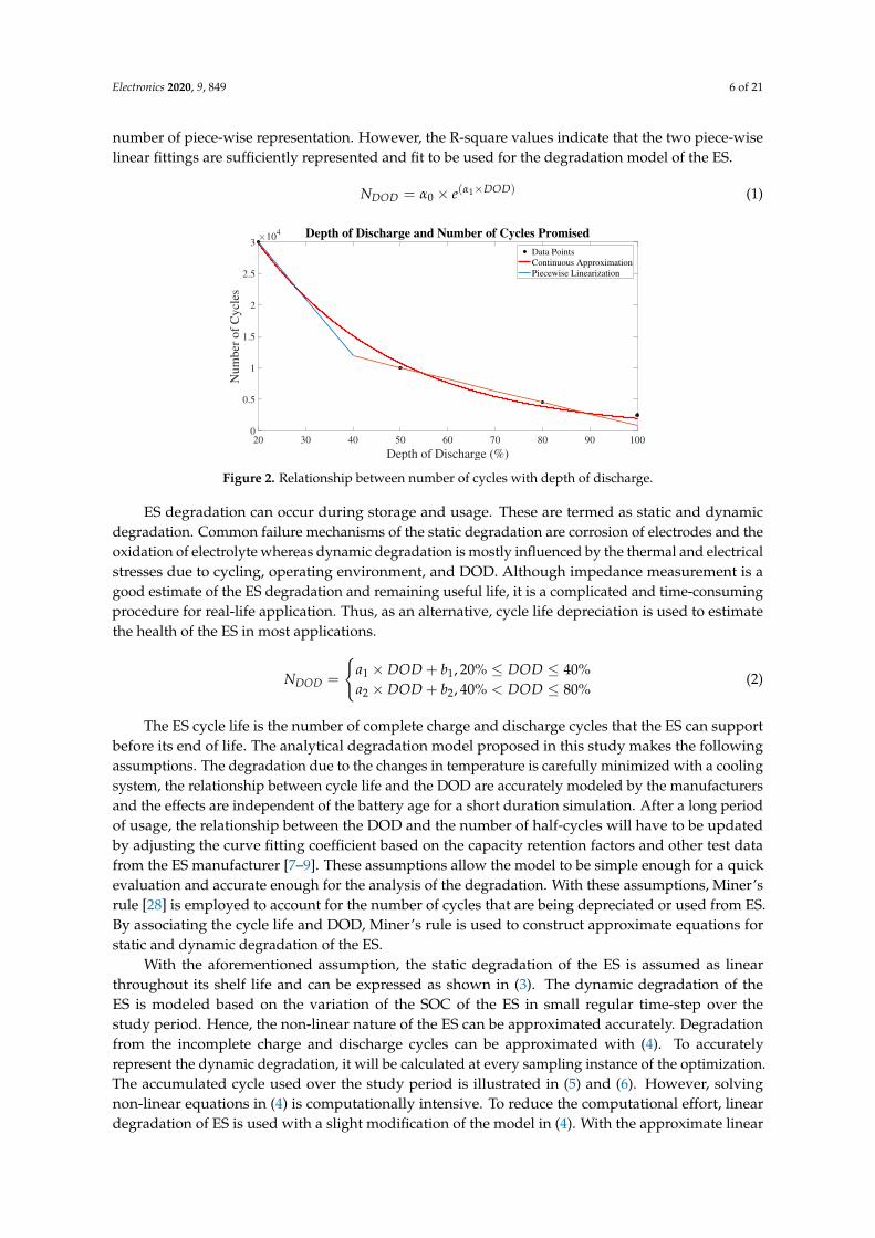
Although it is important to measure the state of health (SOH) of the ES for safe and reliableoperation, it is still a very challenging and complex task due to the complex interaction of the chemistryin ES system. Thus, ES manufacturers generally provide the number of cycles promised and depth ofdischarge (DOD) as the key measures to estimate the SOH of the ES. The number of half-cycles withrespect to the DOD provided by the manufacturer [27] is shown in Figure 2. Exponential curve fitting iscarried out to derive the fitting coefficient to defines the relationship between cycle life and DOD in (1).To reduce the computational effort of non-linear function, Equation (1) is linearized into two piece-wiselinear functions as shown in (2). For the two piece-wise linear functions, the goodness of fits areprovided as R-square values based on the data points given in [27]. The fitting range or the interval ofthe linear functions are also determined based on the R-square values of the fitting. For the piece-wiseapproximation from 20% to 40%, R-square value is 0.9658. Similarly, the piece-wise approximationbetween 40% to 60%, the R-square value is 0.9782. Larger number of piece-wise functions can also beused to represent the relationship between the number of half-cycles and depth of discharge to furtherimprove the accuracy of the approximation without compromising the efficiency of the computationaltime. This is because the search space for the optimal solution remain unchanged with the increase in
Electronics 2020, 9, 849 6 of 21
number of piece-wise representation. However, the R-square values indicate that the two piece-wiselinear fittings are sufficiently represented and fit to be used for the degradation model of the ES.
NDOD = α0 × e(α1×DOD) (1)
20 30 40 50 60 70 80 90 100
Depth of Discharge (%)
0
0.5
1
1.5
2
2.5
3N
um
ber
of
Cy
cles
104 Depth of Discharge and Number of Cycles Promised
Data Points
Continuous Approximation
Piecewise Linearization
Figure 2. Relationship between number of cycles with depth of discharge.
ES degradation can occur during storage and usage. These are termed as static and dynamicdegradation. Common failure mechanisms of the static degradation are corrosion of electrodes and theoxidation of electrolyte whereas dynamic degradation is mostly influenced by the thermal and electricalstresses due to cycling, operating environment, and DOD. Although impedance measurement is agood estimate of the ES degradation and remaining useful life, it is a complicated and time-consumingprocedure for real-life application. Thus, as an alternative, cycle life depreciation is used to estimatethe health of the ES in most applications.
NDOD =
{a1 × DOD + b1, 20% ≤ DOD ≤ 40%a2 × DOD + b2, 40% < DOD ≤ 80%
(2)
The ES cycle life is the number of complete charge and discharge cycles that the ES can supportbefore its end of life. The analytical degradation model proposed in this study makes the followingassumptions. The degradation due to the changes in temperature is carefully minimized with a coolingsystem, the relationship between cycle life and the DOD are accurately modeled by the manufacturersand the effects are independent of the battery age for a short duration simulation. After a long periodof usage, the relationship between the DOD and the number of half-cycles will have to be updatedby adjusting the curve fitting coefficient based on the capacity retention factors and other test datafrom the ES manufacturer [7–9]. These assumptions allow the model to be simple enough for a quickevaluation and accurate enough for the analysis of the degradation. With these assumptions, Miner’srule [28] is employed to account for the number of cycles that are being depreciated or used from ES.By associating the cycle life and DOD, Miner’s rule is used to construct approximate equations forstatic and dynamic degradation of the ES.
With the aforementioned assumption, the static degradation of the ES is assumed as linearthroughout its shelf life and can be expressed as shown in (3). The dynamic degradation of theES is modeled based on the variation of the SOC of the ES in small regular time-step over thestudy period. Hence, the non-linear nature of the ES can be approximated accurately. Degradationfrom the incomplete charge and discharge cycles can be approximated with (4). To accuratelyrepresent the dynamic degradation, it will be calculated at every sampling instance of the optimization.The accumulated cycle used over the study period is illustrated in (5) and (6). However, solvingnon-linear equations in (4) is computationally intensive. To reduce the computational effort, lineardegradation of ES is used with a slight modification of the model in (4). With the approximate linear
Electronics 2020, 9, 849 7 of 21
representation between cycle life and DOD as shown in (2), dynamic degradation per half-cycle fromDOD of i% to j% is linearized as shown in (7).
γs =1
2× Nstatic × tlt,ES× T (3)
γd =T
∑t=2
∣∣∣∣ 12× NDOD(t)
− 12× NDOD(t− 1)
∣∣∣∣ (4)
γacc = γs + γd (5)
tlt,ES
∑t=1
γacc(t) = 1 (6)
γd =12
∣∣∣∣∣ 1NDOD,i%
− 1NDOD,j%
∣∣∣∣∣ , i% ≤ DOD ≤ j% (7)
5.2. Propulsion Load Model
The propulsion load is approximated from a given speed profile. It depends on the resistance ofthe hull and the operating condition of the vessel. It can be approximated with (8) [14,17]. The typicalload profile of a ferry is generally categorized into 5 different operation modes; departing harbor,acceleration, approaching harbor, cruising, and at the harbor. Since ferries tend to follow a regulartravel route, operating speed, and have smaller form factor to have significant effects with propulsionadjustment, voyage scheduling is not carried out in this study.
PPr op = cP1 × vcP2 (8)
5.3. Demand Response Electricity Price Model
S2S is an appropriate solution to make harbors free from greenhouse gas emission and airpollutants while the vessel is at berth. In this study, it is assumed that the shore area is sufficientlydesigned and well-equipped for the S2S power supply and they are directly supplied by the electricityproviders from the main grid. Thus, demand response electricity pricing is modeled for S2S and isillustrated in (9). The grid electricity price is dependent on the amount of electricity acquired from theship power system. The scaling factor ζ is introduced to account for the inflation factor for the serviceprovision from the grid. It can be due to the infrastructure improvement or the grid congestion at thetime of demand. The proposed demand response pricing model is inspired by the demand responsepricing schemes that are implemented in the industry [29].
Fele(t) = fTOU(t)×(
1 + ζ ×Pgrid(t)Pgrid,max
)(9)
5.4. Hybrid Vessel Operation Model
In this study, the objectives of the optimal scheduling of ferries are to reduce the operation cost ofthe ferry such as fuel consumption, maintenance, emission, and grid charging while reducing the ESdegradation. The objectives are categorized to form two conflicting functions that are related by theweighted coefficients; w1 and w2 as shown in (10). The detailed representations of the objectives areillustrated in (11)–(17). For clarity, associative objectives which are weighted with the coefficient w1
and w2 will be termed as objective 1 and objective 2 for the remaining of the paper. It is worthwhileto note that individual weights can be assigned to objective terms from (11)–(17). Nonetheless, it ismore computationally intensive with the increase in number of separate objectives. Hence, based on
Electronics 2020, 9, 849 8 of 21
the prior literature survey and initial simulation results, the cooperative objectives and conflictingobjectives are identified [13,14,17–19].
min w1(cost f uel + costSC/SD + costDGmai + costPV
mai + costgrid + costemission) + w2costESS,deg (10)
cost f uel =T
∑t=1
N
∑n=1
Ff uel × ∆t× FCnDG(t) (11)
costSC/SD =T
∑t=1
N
∑n=1|un
DG(t)− unDG(t + 1)| × Ftrans (12)
costDGmai =
T
∑t=1
N
∑n=1
FDG,mai × PnDG(t)× ∆t (13)
costPVmai =
T
∑t=1
FPV,mai × PPV(t)× ∆t (14)
costgrid =T
∑t=1
Pgrid(t)× Fele(t)× ∆t (15)
costemission =T
∑t=1
N
∑n=1
Fco2 × cco2 × FCnDG(t)× ∆t (16)
costESS,deg = Total Life Cycle Cost×T
∑t=1
γacc (17)
Total Life Cycle Cost = IESS −SlESS
(1 + r)T +T
∑t=1
OMESS
(1 + r)t +T
∑t=1
Fch,ave × Nave × EESS,rated
(1 + r)t (18)
IESS = SESS,rated × EESS,rated (19)
DGs’ fuel consumption is computed with (11). Smaller DGs on ferries tend to have lower statetransition costs. However, to lower the number of state transitions, the total cost of state transitionas shown in (12) is used. The total DGs and PV maintenance cost are illustrated in (13) and (14).The total cost of S2S operation is expressed in (15). The total carbon tax due to emission is calculatedas shown in (16). As shown in (17), total ES degradation cost is modeled as the amount of life cyclecost that is being depreciated from its usage. The total life cycle cost of the ES in (18) is a function ofthe initial investment cost, salvage cost, operation and maintenance cost, and charging cost. The initialinvestment cost as shown in (19) is a one-time cost incurred at the start of the project. In contrast,the operation and maintenance cost (OM) are incurred throughout the operational lifecycle. ES isrequired to be charged for it to be used and the cost of charging is accounted for when calculating thelife cycle cost of the ES. Aggregated average charging price of electricity is used as the future value ofthe grid electricity price. The scaling factor 1/(1+r)t is the conversion factor of the future value to thepresent value in the total life cycle cost calculation.
N
∑i=1
PnDG(t) + Pgrid(t) + Pdis(t) + PPV(t) = Pload(t) + Pch(t) (20)
PnDG,min ≤ Pn
DG(t) ≤ PnDG,max (21)∣∣Pn
DG(t)− PnDG(t− 1)
∣∣∆t
≤ Pnramp,max (22)∣∣∣un
DG(ton/o f f )− unDG(to f f /on)
∣∣∣ ≥ tn,min on/o f fDG (23)
Electronics 2020, 9, 849 9 of 21
Pgrid,min ≤ Pgrid(t) ≤ Pgrid,max (24)
SOCmin ≤ SOC(t) ≤ SOCmax (25)
SOC(t) = SOC(t− 1) +[ηch × Pch(t)× ∆t]−
[Pdis(t)
ηdis× ∆t
]EESS,rated
× 100 (26)
Pch,min × u′ESS(t) ≤ Pch(t) ≤ Pch,max × u
′ESS(t) (27)
Pdis,min × uESS(t) ≤ Pdis(t) ≤ Pdis,max × uESS(t) (28)
FCnDG = an × (Pn
DG)2 + bn × Pn
DG + cn (29)
[PPV,min(t), PPV,max(t)] = ηPV(t)× APV ×[IrrPV,min(t), IrrPV,max(t)
](30)
Mathematical model of the ship power system is employed and the detailed operating constraintof the ship power system is illustrated in this section [13,14,17–19,21–24]. The power balance constraintin the ferry is shown in (20). In (21)–(23), the loading factor, ramp rate and minimum up/downtime constraints of the DGs are specified. Minimum and maximum power exchange with the S2Spower supply are shown in (24). ES SOC limits are specified in (25) and updated with (26). The ESmaximum and minimum charge/discharge power limits are illustrated in (27) and (28). The DGs fuelconsumption which is a factor of loading factor is approximated as shown in (29). PV output based onirradiation is carried out as interval forecast data in this study and illustrated in (30).
6. Solution Methods
The compact form of the solution methods, programming language and solver used are furtherillustrated in this section. The optimization problem is scalarized linearly with the weighted sumapproach in this study. The scalarization of the objective functions in (10) is governed by (31). Due tonon-dominated solutions, the key challenge with the multi-objective problem is to select the operationpoint. Hence, in this study, the mapping of the solution space based on the day-ahead PV predictiondata is carried out to allow the vessel operators to comprehend the operating points prior to the actualoptimal dispatch (hour-ahead). The proposed optimal dispatch problem and solution method aremodel in MATLAB with YALMIP and solve using CPLEX solver [30,31]. Once the Pareto front solutionsets are identified with the iteration process, the multi-objective decision-making process must becarried out to select the optimal trade-off between the objectives. One of the challenges with trade-offanalysis in the multi-objective optimization is that the comparison vectors are non-commensurabledue to the large difference in the numerical value. This can be overcome with the normalization of thesolution vectors (N = [N11,N12, . . . ,Nnm]) over the positive range between 0 and 1 without changingtheir physical meaning or representation. Hence, in this study, normalization is carried out to comparethe Pareto solution sets. Assuming there are n-dimensional Pareto solution sets for m-dimensionobjectives, the normalization of the individual objective criteria can be carried out for each Paretosolution set as shown in (32) [26]. Once the normalization is carried out, the optimal operating pointcan be identified by calculating the Euclidean distance from the user preference operation point.
F(x) =m
∑i=1
wi× fi(x), wi ≥ 0,m
∑i=1
wi = 1 (31)
Ni,j =( fi,j − f j,min)
( f j,max − f j,min);
{i = 1, ..., nj = 1, ..., m
(32)
7. Case Study Parameters
This section will elaborate the vessel under study and its operating parameters to be used for thecase study.
Electronics 2020, 9, 849 10 of 21
7.1. System Configuration and Parameters
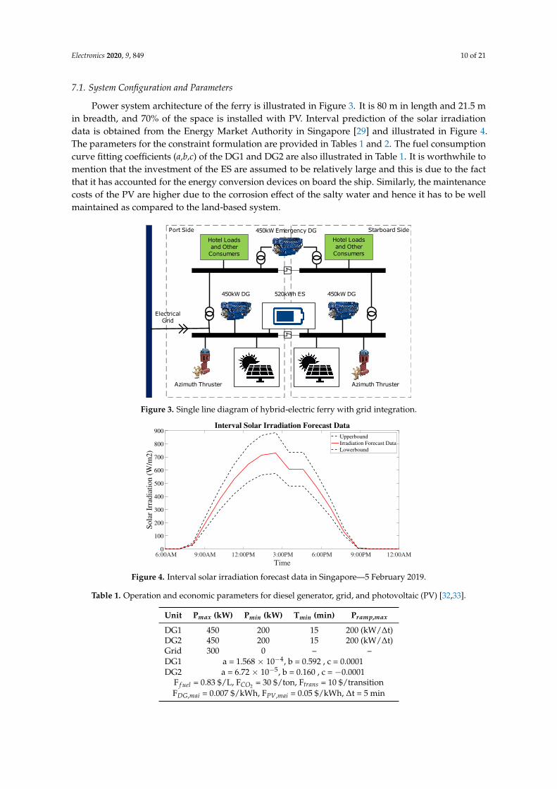
Power system architecture of the ferry is illustrated in Figure 3. It is 80 m in length and 21.5 min breadth, and 70% of the space is installed with PV. Interval prediction of the solar irradiationdata is obtained from the Energy Market Authority in Singapore [29] and illustrated in Figure 4.The parameters for the constraint formulation are provided in Tables 1 and 2. The fuel consumptioncurve fitting coefficients (a,b,c) of the DG1 and DG2 are also illustrated in Table 1. It is worthwhile tomention that the investment of the ES are assumed to be relatively large and this is due to the factthat it has accounted for the energy conversion devices on board the ship. Similarly, the maintenancecosts of the PV are higher due to the corrosion effect of the salty water and hence it has to be wellmaintained as compared to the land-based system.
Azimuth ThrusterAzimuth Thruster
Hotel Loads and Other
Consumers
Hotel Loads and Other
Consumers
Port Side Starboard Side
Electrical Grid
450kW DG450kW DG
450kW Emergency DG
520kWh ES
Figure 3. Single line diagram of hybrid-electric ferry with grid integration.
6:00AM 9:00AM 12:00PM 3:00PM 6:00PM 9:00PM 12:00AM
Time
0
100
200
300
400
500
600
700
800
900
So
lar
Irra
dia
tio
n (
W/m
2)
Interval Solar Irradiation Forecast Data
Upperbound
Irradiation Forecast Data
Lowerbound
Figure 4. Interval solar irradiation forecast data in Singapore—5 February 2019.
Table 1. Operation and economic parameters for diesel generator, grid, and photovoltaic (PV) [32,33].
Unit Pmax (kW) Pmin (kW) Tmin (min) Pramp,max
DG1 450 200 15 200 (kW/∆t)DG2 450 200 15 200 (kW/∆t)Grid 300 0 – –DG1 a = 1.568 × 10⁻⁴, b = 0.592 , c = 0.0001DG2 a = 6.72 × 10⁻⁵, b = 0.160 , c = −0.0001
F f uel = 0.83 $/L, FCO2 = 30 $/ton, Ftrans = 10 $/transitionFDG,mai = 0.007 $/kWh, FPV,mai = 0.05 $/kWh, ∆t = 5 min
Electronics 2020, 9, 849 11 of 21
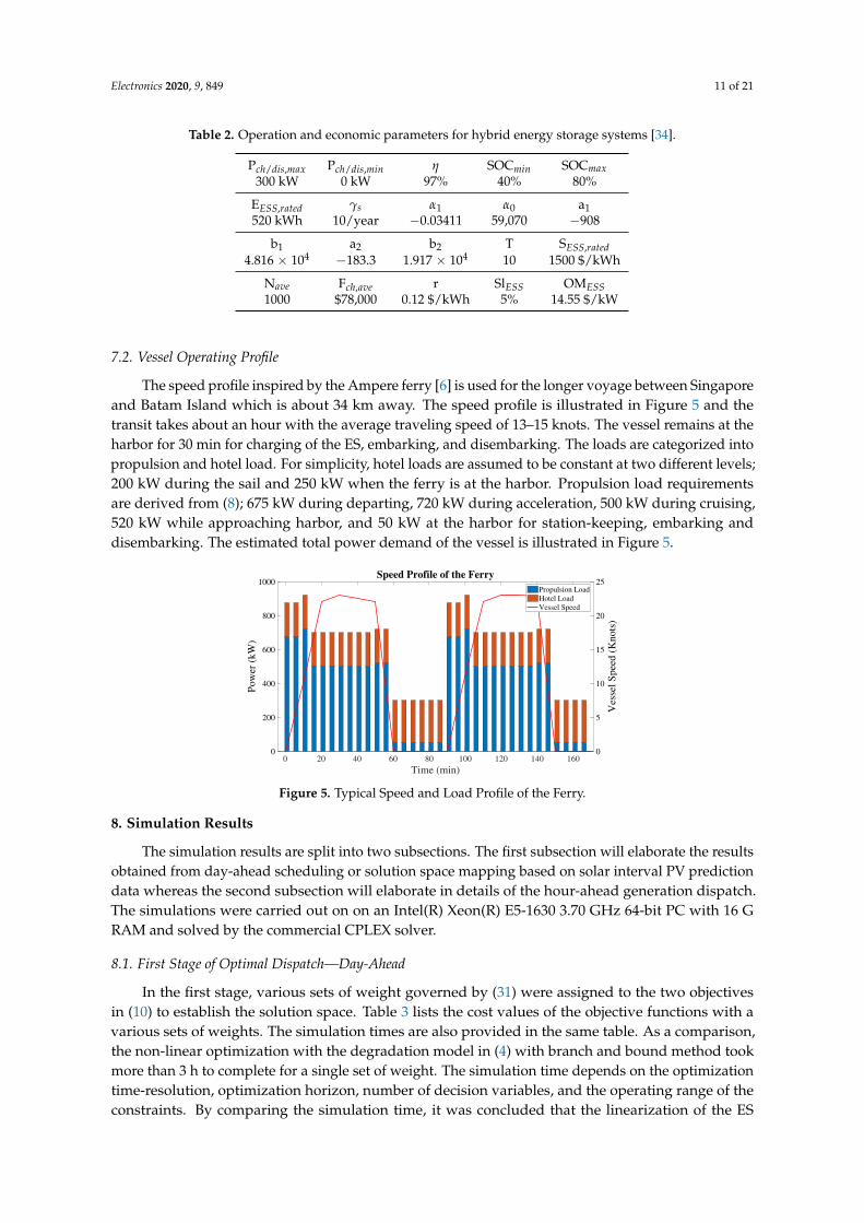
Table 2. Operation and economic parameters for hybrid energy storage systems [34].
Pch/dis,max Pch/dis,min η SOCmin SOCmax300 kW 0 kW 97% 40% 80%
EESS,rated γs α1 α0 a1520 kWh 10/year −0.03411 59,070 −908
b1 a2 b2 T SESS,rated4.816 × 104 −183.3 1.917 × 10⁴ 10 1500 $/kWh
Nave Fch,ave r SlESS OMESS1000 $78,000 0.12 $/kWh 5% 14.55 $/kW
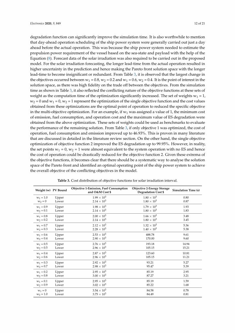
7.2. Vessel Operating Profile
The speed profile inspired by the Ampere ferry [6] is used for the longer voyage between Singaporeand Batam Island which is about 34 km away. The speed profile is illustrated in Figure 5 and thetransit takes about an hour with the average traveling speed of 13–15 knots. The vessel remains at theharbor for 30 min for charging of the ES, embarking, and disembarking. The loads are categorized intopropulsion and hotel load. For simplicity, hotel loads are assumed to be constant at two different levels;200 kW during the sail and 250 kW when the ferry is at the harbor. Propulsion load requirementsare derived from (8); 675 kW during departing, 720 kW during acceleration, 500 kW during cruising,520 kW while approaching harbor, and 50 kW at the harbor for station-keeping, embarking anddisembarking. The estimated total power demand of the vessel is illustrated in Figure 5.
0
5
10
15
20
25
Ves
sel
Sp
eed
(K
no
ts)
Speed Profile of the Ferry
0 20 40 60 80 100 120 140 160
Time (min)
0
200
400
600
800
1000
Po
wer
(k
W)
Propulsion Load
Hotel Load
Vessel Speed
Figure 5. Typical Speed and Load Profile of the Ferry.
8. Simulation Results
The simulation results are split into two subsections. The first subsection will elaborate the resultsobtained from day-ahead scheduling or solution space mapping based on solar interval PV predictiondata whereas the second subsection will elaborate in details of the hour-ahead generation dispatch.The simulations were carried out on on an Intel(R) Xeon(R) E5-1630 3.70 GHz 64-bit PC with 16 GRAM and solved by the commercial CPLEX solver.
8.1. First Stage of Optimal Dispatch—Day-Ahead
In the first stage, various sets of weight governed by (31) were assigned to the two objectivesin (10) to establish the solution space. Table 3 lists the cost values of the objective functions with avarious sets of weights. The simulation times are also provided in the same table. As a comparison,the non-linear optimization with the degradation model in (4) with branch and bound method tookmore than 3 h to complete for a single set of weight. The simulation time depends on the optimizationtime-resolution, optimization horizon, number of decision variables, and the operating range of theconstraints. By comparing the simulation time, it was concluded that the linearization of the ES
Electronics 2020, 9, 849 12 of 21
degradation function can significantly improve the simulation time. It is also worthwhile to mentionthat day-ahead operation scheduling of the ship power system were generally carried out just a dayahead before the actual operation. This was because the ship power system needed to estimate thepropulsion power requirement of the vessel based on the sea-state and payload with the help of theEquation (8). Forecast data of the solar irradiation was also required to be carried out in the proposedmodel. For the solar irradiation forecasting, the longer lead-time from the actual operation resulted inhigher uncertainty in the prediction and hence making the Pareto front solution space with the longerlead-time to become insignificant or redundant. From Table 3, it is observed that the largest change inthe objectives occurred between w1 = 0.8, w2 = 0.2 and w1 = 0.6, w2 = 0.4. It is the point of interest in thesolution space, as there was high fidelity on the trade off between the objectives. From the simulationtime as shown in Table 3, it also reflected the conflicting nature of the objective functions at these sets ofweight as the computation time of the optimization significantly increased. The set of weights w1 = 1,w2 = 0 and w1 = 0, w2 = 1 represent the optimization of the single objective function and the cost valuesobtained from these optimizations are the optimal point of operation to reduced the specific objectivein the multi-objective optimization. For an example, if w1 was assigned a value of 1, the minimum costof emission, fuel consumption, and operation cost and the maximum value of ES degradation wereobtained from the above optimization. These sets of weights could be used as benchmarks to evaluatethe performance of the remaining solution. From Table 3, if only objective 1 was optimized, the cost ofoperation, fuel consumption and emission improved up to 46.93%. This is proven in many literaturethat are discussed in detailed in the literature review section. On the other hand, the single objectiveoptimization of objective function 2 improved the ES degradation up to 99.95%. However, in reality,the set points w1 = 0, w2 = 1 were almost equivalent to the system operation with no ES and hencethe cost of operation could be drastically reduced for the objective function 2. Given these extrema ofthe objective functions, it becomes clear that there should be a systematic way to analyse the solutionspace of the Pareto front and identified an optimal operating point of the ship power system to achievethe overall objective of the conflicting objectives in the model.
Table 3. Cost distribution of objective functions for solar irradiation interval.
Weight (w) PV Bound Objective 1-Emission, Fuel Consumptionand O&M Cost $
Objective 2-Energy StorageDegradation Cost $ Simulation Time (s)
w1 = 1.0w2 = 0
Upper 1.99 × 10³ 1.80 × 10³ 0.80Lower 2.14 × 10³ 1.80 × 10³ 0.87
w1 = 0.9w2 = 0.1
Upper 1.98 × 10³ 1.79 × 10³ 1.93Lower 2.14 × 10³ 1.80 × 10³ 1.83
w1 = 0.8w2 = 0.2
Upper 2.00 × 10³ 1.66 × 10³ 3.48Lower 2.14 × 10³ 1.80 × 10³ 3.45
w1 = 0.7w2 = 0.3
Upper 2.12 × 10³ 1.32 × 10³ 5.36Lower 2.28 × 10³ 1.40 × 10³ 5.38
w1 = 0.6w2 = 0.4
Upper 2.53 × 10³ 488.78 9.61Lower 2.90 × 10³ 170.00 9.60
w1 = 0.5w2 = 0.5
Upper 2.76 × 10³ 193.18 14.94Lower 2.96 × 10³ 105.15 15.21
w1 = 0.4w2 = 0.6
Upper 2.87 × 10³ 123.60 10.81Lower 2.96 × 10³ 105.15 11.21
w1 = 0.3w2 = 0.7
Upper 2.92 × 10³ 93.21 5.27Lower 2.98 × 10³ 95.47 5.39
w1 = 0.2w2 = 0.8
Upper 2.95 × 10³ 85.19 2.95Lower 3.00 × 10³ 87.27 3.21
w1 = 0.1w2 = 0.9
Upper 2.95 × 10³ 85.19 1.59Lower 3.02 × 10³ 85.22 1.68
w1 = 0w2 = 1.0
Upper 3.54 × 10³ 84.58 0.78Lower 3.75 × 10³ 84.49 0.81
Electronics 2020, 9, 849 13 of 21
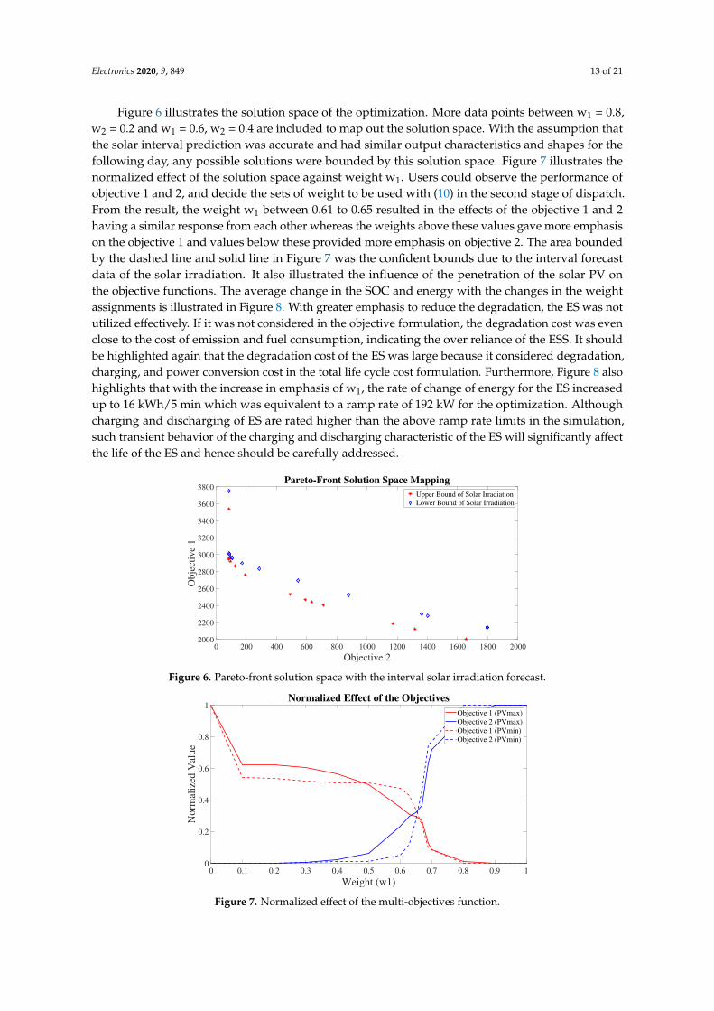
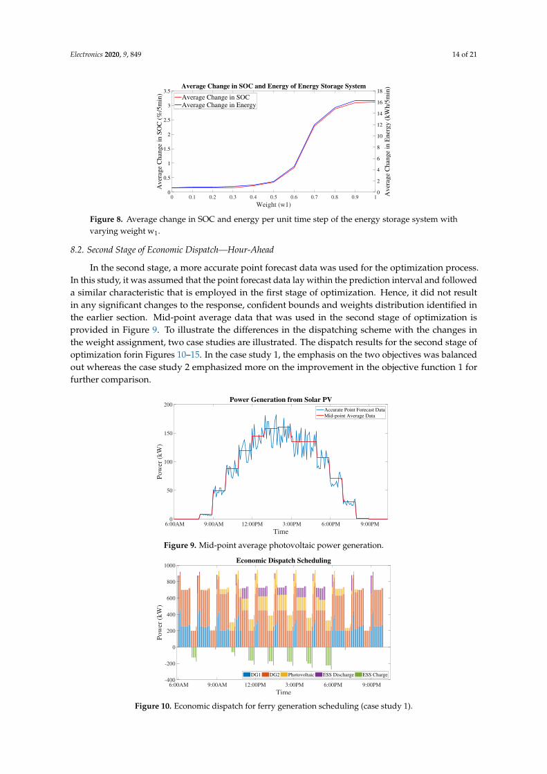
Figure 6 illustrates the solution space of the optimization. More data points between w1 = 0.8,w2 = 0.2 and w1 = 0.6, w2 = 0.4 are included to map out the solution space. With the assumption thatthe solar interval prediction was accurate and had similar output characteristics and shapes for thefollowing day, any possible solutions were bounded by this solution space. Figure 7 illustrates thenormalized effect of the solution space against weight w1. Users could observe the performance ofobjective 1 and 2, and decide the sets of weight to be used with (10) in the second stage of dispatch.From the result, the weight w1 between 0.61 to 0.65 resulted in the effects of the objective 1 and 2having a similar response from each other whereas the weights above these values gave more emphasison the objective 1 and values below these provided more emphasis on objective 2. The area boundedby the dashed line and solid line in Figure 7 was the confident bounds due to the interval forecastdata of the solar irradiation. It also illustrated the influence of the penetration of the solar PV onthe objective functions. The average change in the SOC and energy with the changes in the weightassignments is illustrated in Figure 8. With greater emphasis to reduce the degradation, the ES was notutilized effectively. If it was not considered in the objective formulation, the degradation cost was evenclose to the cost of emission and fuel consumption, indicating the over reliance of the ESS. It shouldbe highlighted again that the degradation cost of the ES was large because it considered degradation,charging, and power conversion cost in the total life cycle cost formulation. Furthermore, Figure 8 alsohighlights that with the increase in emphasis of w1, the rate of change of energy for the ES increasedup to 16 kWh/5 min which was equivalent to a ramp rate of 192 kW for the optimization. Althoughcharging and discharging of ES are rated higher than the above ramp rate limits in the simulation,such transient behavior of the charging and discharging characteristic of the ES will significantly affectthe life of the ES and hence should be carefully addressed.
0 200 400 600 800 1000 1200 1400 1600 1800 2000
Objective 2
2000
2200
2400
2600
2800
3000
3200
3400
3600
3800
Obje
ctiv
e 1
Pareto-Front Solution Space Mapping
Upper Bound of Solar Irradiation
Lower Bound of Solar Irradiation
Figure 6. Pareto-front solution space with the interval solar irradiation forecast.
0 0.1 0.2 0.3 0.4 0.5 0.6 0.7 0.8 0.9 1
Weight (w1)
0
0.2
0.4
0.6
0.8
1
Norm
aliz
ed V
alue
Normalized Effect of the Objectives
Objective 1 (PVmax)
Objective 2 (PVmax)
Objective 1 (PVmin)
Objective 2 (PVmin)
Figure 7. Normalized effect of the multi-objectives function.
Electronics 2020, 9, 849 14 of 21
0 0.1 0.2 0.3 0.4 0.5 0.6 0.7 0.8 0.9 1
Weight (w1)
0
0.5
1
1.5
2
2.5
3
3.5
Aver
age
Chan
ge
in S
OC
(%
/5m
in)
0
2
4
6
8
10
12
14
16
18
Aver
age
Chan
ge
in E
ner
gy (
kW
h/5
min
)Average Change in SOC and Energy of Energy Storage System
Average Change in SOCAverage Change in Energy
Figure 8. Average change in SOC and energy per unit time step of the energy storage system withvarying weight w1.
8.2. Second Stage of Economic Dispatch—Hour-Ahead
In the second stage, a more accurate point forecast data was used for the optimization process.In this study, it was assumed that the point forecast data lay within the prediction interval and followeda similar characteristic that is employed in the first stage of optimization. Hence, it did not resultin any significant changes to the response, confident bounds and weights distribution identified inthe earlier section. Mid-point average data that was used in the second stage of optimization isprovided in Figure 9. To illustrate the differences in the dispatching scheme with the changes inthe weight assignment, two case studies are illustrated. The dispatch results for the second stage ofoptimization forin Figures 10–15. In the case study 1, the emphasis on the two objectives was balancedout whereas the case study 2 emphasized more on the improvement in the objective function 1 forfurther comparison.
6:00AM 9:00AM 12:00PM 3:00PM 6:00PM 9:00PM
Time
0
50
100
150
200
Pow
er (
kW
)
Power Generation from Solar PV
Accurate Point Forecast Data
Mid-point Average Data
Figure 9. Mid-point average photovoltaic power generation.
Economic Dispatch Scheduling
6:00AM 9:00AM 12:00PM 3:00PM 6:00PM 9:00PM
Time
-400
-200
0
200
400
600
800
1000
Pow
er (
kW
)
DG1 DG2 Photovoltaic ESS Discharge ESS Charge
Figure 10. Economic dispatch for ferry generation scheduling (case study 1).
Electronics 2020, 9, 849 15 of 21
0.06
0.062
0.064
0.066
0.068
0.07
0.072
0.074
0.076
0.078
Gri
d E
lect
rici
ty P
rice
($
/kW
h)
Demand Response Grid Electricity Price
6:00AM 9:00AM 12:00PM 3:00PM 6:00PM 9:00PM
Time
0
50
100
150
200
250
300
Po
wer
(k
W)
Grid Power SuppliedGrid Electricity PricePeak Demand Electricity Price
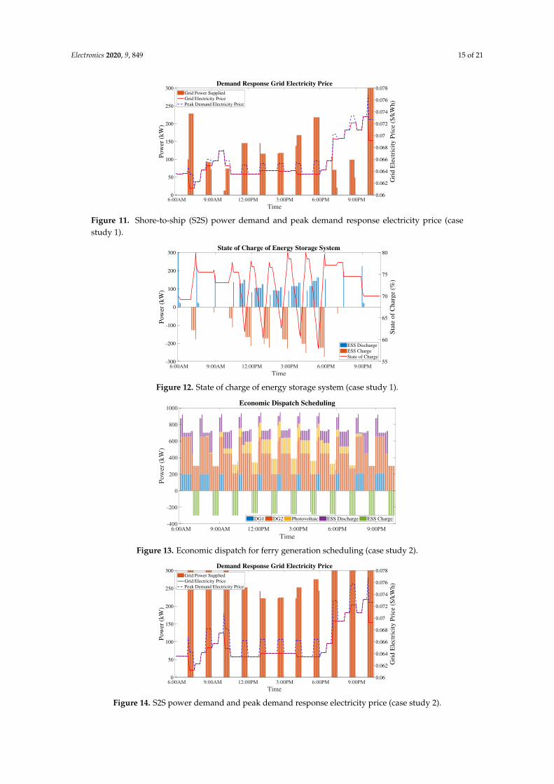
Figure 11. Shore-to-ship (S2S) power demand and peak demand response electricity price (casestudy 1).
55
60
65
70
75
80
Sta
te o
f C
har
ge
(%)
State of Charge of Energy Storage System
6:00AM 9:00AM 12:00PM 3:00PM 6:00PM 9:00PM
Time
-300
-200
-100
0
100
200
300
Po
wer
(k
W)
ESS Discharge
ESS Charge
State of Charge
Figure 12. State of charge of energy storage system (case study 1).
Economic Dispatch Scheduling
6:00AM 9:00AM 12:00PM 3:00PM 6:00PM 9:00PM
Time
-400
-200
0
200
400
600
800
1000
Po
wer
(kW
)
DG1 DG2 Photovoltaic ESS Discharge ESS Charge
Figure 13. Economic dispatch for ferry generation scheduling (case study 2).
0.06
0.062
0.064
0.066
0.068
0.07
0.072
0.074
0.076
0.078
Gri
d E
lect
rici
ty P
rice
($
/kW
h)
Demand Response Grid Electricity Price
6:00AM 9:00AM 12:00PM 3:00PM 6:00PM 9:00PM
Time
0
50
100
150
200
250
300
Po
wer
(k
W)
Grid Power SuppliedGrid Electricity PricePeak Demand Electricity Price
Figure 14. S2S power demand and peak demand response electricity price (case study 2).
Electronics 2020, 9, 849 16 of 21
40
45
50
55
60
65
70
75
80
Sta
te o
f C
har
ge
(%)
State of Charge of Energy Storage System
6:00AM 9:00AM 12:00PM 3:00PM 6:00PM 9:00PM
Time
-300
-200
-100
0
100
200
300
Pow
er (
kW
)
ESS Discharge
ESS Charge
State of Charge
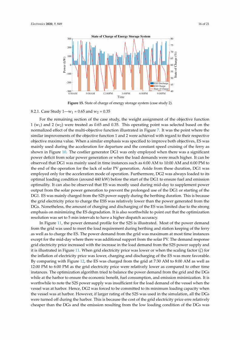
Figure 15. State of charge of energy storage system (case study 2).
8.2.1. Case Study 1—w1 = 0.65 and w2 = 0.35
For the remaining section of the case study, the weight assignment of the objective function1 (w1) and 2 (w2) were treated as 0.65 and 0.35. This operating point was selected based on thenormalized effect of the multi-objective function illustrated in Figure 7. It was the point where thesimilar improvements of the objective function 1 and 2 were achieved with regard to their respectiveobjective maxima value. When a similar emphasis was specified to improve both objectives, ES wasmainly used during the acceleration for departure and the constant speed cruising of the ferry asshown in Figure 10. The costlier generator DG1 was only employed when there was a significantpower deficit from solar power generation or when the load demands were much higher. It can beobserved that DG1 was mainly used in time instances such as 6:00 AM to 10:00 AM and 6:00 PM tothe end of the operation for the lack of solar PV generation. Aside from these duration, DG1 wasemployed only for the acceleration mode of operation. Furthermore, DG2 was always loaded to itsoptimal loading condition (around 440 kW) before the start of the DG1 to ensure fuel and emissionoptimality. It can also be observed that ES was mostly used during mid-day to supplement poweroutput from the solar power generation to prevent the prolonged use of the DG1 or starting of theDG1. ES was mainly charged from the S2S power supply during the berthing duration. This is becausethe grid electricity price to charge the ESS was relatively lower than the power generated from theDGs. Nonetheless, the amount of charging and discharging of the ES was limited due to the strongemphasis on minimizing the ES degradation. It is also worthwhile to point out that the optimizationresolution was set to 5 min intervals to have a higher dispatch accuracy.
In Figure 11, the power demand profile for the S2S is illustrated. Most of the power demandfrom the grid was used to meet the load requirement during berthing and station keeping of the ferryas well as to charge the ES. The power demand from the grid was maximum at most time instancesexcept for the mid-day where there was additional support from the solar PV. The demand responsegrid electricity price increased with the increase in the load demand from the S2S power supply andit is illustrated in Figure 11. When grid electricity price was lower or when the scaling factor (ζ) forthe inflation of electricity price was lower, charging and discharging of the ES was more favorable.By comparing with Figure 12, the ES was charged from the grid at 7:30 AM to 8:00 AM as well as12:00 PM to 6:00 PM as the grid electricity price were relatively lower as compared to other timeinstances. The optimization algorithm tried to balance the power demand from the grid and the DGswhile at the harbor to ensure the economic benefit, fuel consumption, and emission minimization. It isworthwhile to note the S2S power supply was insufficient for the load demand of the vessel when thevessel was at harbor. Hence, DG2 was forced to be committed to its minimum loading capacity whenthe vessel was at harbor. However, if larger rating of the S2S was used in the simulation, all the DGswere turned off during the harbor. This is because the cost of the grid electricity price erre relativelycheaper than the DGs and the emission resulting from the low loading condition of the DGs was
Electronics 2020, 9, 849 17 of 21
unfavourable. It can also be observed that the demand from the grid was lowered when there wassignificant support from the solar PV generation. From Figure 12, it can be observed that the ES wasmainly used during mid-day. As elaborated earlier, it was used as a supplement to the power outputfrom the solar power generation to prevent the starting of DG1. It is also worth noting that the SOCof the ES was maintained above 55% and hence the DOD of the ES was within the healthier rangeof operation. Furthermore, 55% of the energy from the ES was ensured as the energy reserve for theemergency operation conditions. Hence, it can be concluded from the detailed simulation results thatthe dispatch results were highly influenced by many factors and the proposed scheme allowed the shipoperators to have more flexibility in their optimal dispatch while providing a better understandingof the trade-off in the objectives of the chosen dispatch scheme. For the above weight distribution,the cost distributions of objective functions 1 and 2 were 2.54 × 10³ and 632.27. It also means thatthe improvements of the objective functions 1 and 2 were 28.25% and 64.9% improvement from theirrespective maxima values. By comparing with the single objective optimization results illustrated inSection 8.1, it was proven that the optimal trade off between the two objective functions was achievedbased on the weights distribution of the objective functions and updated solar PV irradiation data.Hence, the results obtained are satisfactory for the overall vessel operation.
8.2.2. Case Study 2—w1 = 0.85 and w2 = 0.15
To compare and appreciate the results obtained from the case study 1, case study 2 which isgenerally aligned with what is currently done in the literature is presented. Case study 2 emphasizedmore on the optimization of operation cost, fuel consumption, and emission tax. When more emphasiswas being paid to the objective function 1, it was observed that the economic dispatch utilized theES more frequently. In most of the operation scenarios, instead of turning on the more costly DG1,ES was more frequently used with greater charge and discharge cycles to supply the load demand.The comparison between Figures 10 and 13 illustrates that the number of operation hours of theDG1 was significantly reduced. As illustrated in Figure 14, the greater reliance of the ES resulted inthe higher S2S power demand to charge the ES. The power demand from the S2S was maximum atmost time instances except for mid-day where there was additional support from the solar PV powergeneration. The demand response electricity price for this case study is also illustrated in Figure 14.As compared to Figure 11 in case study 1, the demand response electricity price was higher due to thehigher power demand from the vessel. As the emphasis was to minimize the fuel consumption andoperation cost minimization in the case study 2, the ES was much more frequently exploited. As aresult, a higher number of charge and discharge cycles were being consumed as shown in Figure 15.Furthermore, the DOD and the number of operating hours for the ES are also significantly increasedas compared to Figure 12. It is also observed that, the economic dispatch tried to charge the ESback to higher SOC whenever it was at the harbor for the upcoming operation tasks. In this study,the cost values of the objective functions 1 and 2 were 2.07 × 10³ and 1.75 × 10³. It also meant thatthe improvements of the objective function 1 and 2 were 44.8% and 2.78% improvement from theirrespective maxima values presented in Table 3. If the results are to be compared with the case study 1,it is observed that the operation cost, fuel, and emission efficiency improved from 28.25% to 44.78%which is close to the absolute optimality of the objective function 1. However, with regard to the ESdegradation improvement, it only accounted for 2.78% improvement from its maximum value. Hence,the comparison between case study 1 and 2 has proven that such weight assignments will result in theunbalanced emphasis on the conflicting objective functions and the proposed method in this study hascarefully developed a method to address such potential issues.
In this study, the optimization time horizon for the hour-ahead optimal scheduling remained at24 h. In reality, to achieve a more accurate dispatch, the optimization horizon could be reduced to anhourly or half-day dispatch. With the updated prediction of the solar PV outputs, the objective weightsets could be updated accordingly based on the comparison study that was carried out in the first
Electronics 2020, 9, 849 18 of 21
stage (day-ahead) scheduling. Hence, the proposed methods provided additional flexibility to thesystem operation of the vessel by providing a holistic representation of the dispatching scheme.
9. Conclusions
The study proposed the optimal scheduling of the ferry with the multi-objective functions.It addresses two conflicting objectives in the problem formulation; operation cost which accountsfor fuel cost, CO2 emission cost, grid charging cost, and maintenance cost while minimizing thedegradation of the ES. The multi-objective optimization is solved with the proposed two-stageeconomic dispatch scheme. For the interval forecast data, Pareto-front solution spaces are mappedout to estimate the optimal sets of weight for the two objectives based on the user’s preferencedue to the large difference in the numerical scale. Case studies with different sets of weights areillustrated to demonstrate the effectiveness of the proposed approach in the optimal scheduling ofthe ferry. The main conclusions from this research work are summarized as follows. (1) Due tothe complexity of the model formulation and present of non-linear constraints, linearization of theconstraints such as ES degradation can improve the computation efficiency to map-out the Paretofront solution space as well as to compute the hour-ahead dispatch. The simulation times are withinseconds and hence the applicability of the proposed method for actual implementation can be assured.(2) The proposed method addresses the uncertainty present in the solar PV forecasting by mappingout the Pareto front solution space for the boundary conditions of the solar PV generation to have abetter understanding of the solution space shift for the decision making in hour-ahead scheduling.The simulation results indicate that the higher penetration of solar PV will result in the higher Paretofront shift. Without understanding the solution space, optimal dispatch of the ES and generationsources can not be assured. (3) The results also indicated that with the proper ES management, the DODof the ES can be effectively controlled by the vessel operator by adjusting the weight set points for theobjective functions. From the observation of the average rate of change of energy in ES in Figure 8,the vessel operator can set the ramp rate limit of the ES to ensure the safe operation of the ES. Similar,fuel consumption and operation cost optimization can be done simultaneously with the proper setsof weight assignment for the objective functions. (4) The results also clearly indicate the influenceof demand response grid electricity pricing scheme and the amount of solar PV generation on thepower exchange with the S2S power supply. It is also observed that ESs are mainly charged from thegrid especially when the grid electricity prices are lower. (5) The proposed two-stage multi-objectiveoptimization method improve the accuracy of the generation dispatch result by employing highertime-resolution optimization only when the uncertainty is realized in the hour-ahead scheduling.In the future, more efforts can be spent on integrating more objectives such as thermal performance ofthe ES in the optimization framework.
Author Contributions: Conceptualization, K.H., X.Y. and G.W.; formal analysis, K.H., X.Y. and G.W.; investigation,K.H., X.Y. and G.W.; methodology, K.H., X.Y. and G.W.; validation, K.H., X.Y. and G.W.; visualization, X.Y. andG.W.; writing—original draft, K.H., X.Y. and G.W.; writing—review and editing, K.H., X.Y. and G.W. All authorshave read and agreed to the published version of the manuscript.
Funding: This research received no external funding.The APC for this paper is waived by the guest editor.
Conflicts of Interest: The authors declare no conflict of interest.
Electronics 2020, 9, 849 19 of 21
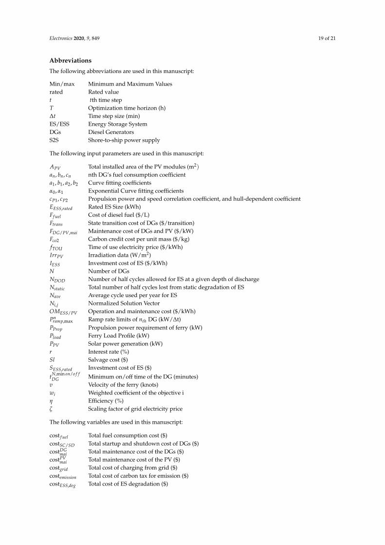
Abbreviations
The following abbreviations are used in this manuscript:
Min/max Minimum and Maximum Valuesrated Rated valuet tth time stepT Optimization time horizon (h)∆t Time step size (min)ES/ESS Energy Storage SystemDGs Diesel GeneratorsS2S Shore-to-ship power supply
The following input parameters are used in this manuscript:
APV Total installed area of the PV modules (m2)
an, bn, cn nth DG’s fuel consumption coefficienta1, b1, a2, b2 Curve fitting coefficientsα0, α1 Exponential Curve fitting coefficientscP1, cP2 Propulsion power and speed correlation coefficient, and hull-dependent coefficientEESS,rated Rated ES Size (kWh)Ff uel Cost of diesel fuel ($/L)Ftrans State transition cost of DGs ($/transition)FDG/PV,mai Maintenance cost of DGs and PV ($/kW)Fco2 Carbon credit cost per unit mass ($/kg)fTOU Time of use electricity price ($/kWh)IrrPV Irradiation data (W/m2)IESS Investment cost of ES ($/kWh)N Number of DGsNDOD Number of half cycles allowed for ES at a given depth of dischargeNstatic Total number of half cycles lost from static degradation of ESNave Average cycle used per year for ESNi,j Normalized Solution VectorOMESS/PV Operation and maintenance cost ($/kWh)Pn
ramp,max Ramp rate limits of nth DG (kW/∆t)PProp Propulsion power requirement of ferry (kW)Pload Ferry Load Profile (kW)PPV Solar power generation (kW)r Interest rate (%)Sl Salvage cost ($)SESS,rated Investment cost of ES ($)
tN,min on/o f fDG Minimum on/off time of the DG (minutes)
v Velocity of the ferry (knots)wi Weighted coefficient of the objective iη Efficiency (%)ζ Scaling factor of grid electricity price
The following variables are used in this manuscript:
cost f uel Total fuel consumption cost ($)costSC/SD Total startup and shutdown cost of DGs ($)costDG
mai Total maintenance cost of the DGs ($)costPV
mai Total maintenance cost of the PV ($)costgrid Total cost of charging from grid ($)costemission Total cost of carbon tax for emission ($)costESS,deg Total cost of ES degradation ($)
Electronics 2020, 9, 849 20 of 21
FCnDG Fuel Consumption of nth DG (liter/kW)
Fele Demand response electricity price ($/kWh)fi,j Objective function j in ith solution set ($)Pn
DG Output power of nth DG (kW)Pgrid Power supplied from the grid (kW)Pch/dis Charge and discharge power from ES (kW)SOC State of Charge of ES (%)tlt,ESS Lifetime of ES (years)un
DG Binary on/off status of the DGun
DG(ton/o f f ) State transition time instance on to offun
DG(to f f /on) State transition time instance off to onγs Static degradation of ESγd Dynamic degradation of ESγacc Accumulated degradation of ES
References
1. International Maritime Organization. Third IMO GHG Study 2014 Executive Summary and Final Reports;International Maritime Organization: London, UK, 2015.
2. European Commission. EU Strategy for Liquefied Natural Gas and Gas Storage; European Commission: Brussels,Belgium, 2016.
3. International Maritime Organization. Prevention of Air Pollution from Ships MARPOL ANNEX VL;International Maritime Organization: London, UK, 1997.
4. International Maritime Organization. Energy Efficiency Measures—Amendments MARPOL ANNEX VL;International Maritime Organization: London, UK, 2013.
5. European Commission. Roadmap to a Single European Transport Area—Towards a Competitive and ResourceEfficient Transport System; European Commission: Brussels, Belgium, 2011.
6. Corvus Energy. World’s First All-Electric Car Ferry—Vessels and Shore Charging Stations. Available online:https://corvusenergy.com/ (accessed on 5 April 2020).
7. Koller, M.; Borsche, T.; Ulbig, A.; Andersson, G. Defining a degradation cost function for optimal control ofa battery energy storage system. In Proceedings of the 2013 IEEE Grenoble Conference, Grenoble, France,16-20 June 2013; pp. 1–6.
8. Perez, A.; Moreno, R.; Moreira, R.; Orchard, M.; Strbac, G. Effect of Battery Degradation on Multi-ServicePortfolios of Energy Storage. IEEE Trans. Sustain. Energy 2016, 7, 1718–1729.
9. Abdulla, K.; De Hoog, J.; Muenzel, V.; Suits, F.; Steer, K.; Wirth, A.; Halgamuge, S. Optimal Operationof Energy Storage Systems Considering Forecasts and Battery Degradation. IEEE Trans. Smart Grid 2018,9, 2086–2096.
10. Ju, C.; wang, P.; Goel, L.; Xu, Y. A two-layer energy management system for microgrid with hybrid energystorage considering degradation costs. IEEE Trans. Smart Grid 2018, 9, 6047–6057.
11. Kumar, J.; Kumpulainen, L.; Kauhaniemi, K. Technical design aspects of harbour area grid for shore to shippower: State of the art and future solutions. Int. J. Electr. Power Energy Syst. 2019, 104, 840–852.
12. Sciberras, EA.; Zahawi, B.; Atkinson, D.J. Reducing shipboard emissions—Assessment of the role of electricaltechnologies. Transp. Res. Part D Transp. Environ. 2017; 51, 227–239.
13. Kanellos, F.D.; Prousalidis, J.M.; Tsekouras, G.J. Control system for fuel consumption minimization-gasemission limitation of full electric propulsion ship power systems. Proc. Inst. Mech. Eng. Part M J. Eng.Marit. Environ. 2014, 228, 17–28.
14. Shang, C.; Srinivasan, D.; Reindl, T. Economic and Environmental Generation and Voyage Scheduling ofAll-Electric Ships. IEEE Trans. Power Syst. 2016 31, 4087–4096.
15. Boveri, A.; Silvestro, F.; Molinas, M.; Skjong, E. Optimal Sizing of Energy Storage Systems for ShipboardApplications. IEEE Trans. Energy Convers. 2018, 34, 801–811.
16. Yao, C.; Chen, M.; Hong, Y.Y. Novel Adaptive Multi-Clustering Algorithm-Based Optimal ESS Sizing in ShipPower System Considering Uncertainty. IEEE Trans. Power Syst. 2018 33, 307–316.

Electronics 2020, 9, 849 21 of 21
17. Shang, C.; Srinivasan, D.; Reindl, T. NSGA-II for joint generation and voyage scheduling of an all-electricship. In Proceedings of the 2016 IEEE Congress on Evolutionary Computation (CEC), Vancouver, BC, Canada,24–29 July 2016.
18. Jaurola, M.; Hedin, A.; Tikkanen, S.; Huhtala, K. Optimising design and power management inenergy-efficient marine vessel power systems: A literature review. J. Mar. Eng. Technol. 2018, 18, 92–101.
19. Kanellos, F.; Anvari-Moghaddam, A.; Guerrero, J. Smart Shipboard Power System Operation andManagement. Inventions 2016, 18, 92–101.
20. Hein, K.; Xu, Y. Hybrid Energy Storage System in Naval Vessel with 2-Stage Power-sharing Algorithm.In Proceedings of the 2019 IEEE Innovative Smart Grid Technologies - Asia (ISGT Asia), Chengdu, China,21–24 May 2019; pp. 3607–3612.
21. Kanellos, F.D. Optimal power management with GHG emissions limitation in all-electric ship power systemscomprising energy storage systems. IEEE Trans. Power Syst. 2014, 29, 330–339.
22. Al-Falahi, M.D.A.; Nimma, K.S.; Jayasinghe, S.D.G.; Enshaei, H.; Guerrero, J.M. Power managementoptimization of hybrid power systems in electric ferries. Energy Convers. Manag. 2018, 172, 50–66.
23. Wen, S.; Lan, H.; Hong, Y.Y.; Yu, D.C.; Zhang, L.; Cheng, P. Allocation of ESS by interval optimizationmethod considering impact of ship swinging on hybrid PV/diesel ship power system. Appl. Energy 2016,175, 158–167.
24. Kanellos, F.D.; Tsekouras, G.J.; Hatziargyriou, N.D. Optimal demand-side management and powergeneration scheduling in an all-electric ship. IEEE Trans. Sustain. Energy 2014, 5, 1166–1175.
25. Huang, Y.; Lan, H.; Hong, Y.Y.; Wen, S.; Fang, S. Joint voyage scheduling and economic dispatch forall-electric ships with virtual energy storage systems. Energy 2020, 190, 116268.
26. Zhengmao, L.; Yan, X.; Sidun, F.; Yu, W. Multi-objective Coordinated Energy Dispatch and Voyage Schedulingfor a Multi-energy Cruising Ship. In Proceedings of the 2019 IEEE/IAS 55th Industrial and CommercialPower Systems Technical Conference (I&CPS), Calgary, AB, Canada, 5–8 May 2019; pp. 1-8.
27. LithiumWerks. Lithium Phosphate Battery. Available online: https://lithiumwerks.com/technology/(accessed on 5 April 2020).
28. Miner, M.A. Cumulative damage in fatigue J. Appl. Mech. 1945, 12, 159–164.29. Energy Market Authority. Renewable Energy: Solar Generation Profile. Available online: https://www.ema.
gov.sg/Renewable_Energy.aspx (accessed on 5 April 2020).30. Lofberg, J. YALMIP: A toolbox for modeling and optimization in MATLAB. In Proceedings of the 2004 IEEE
International Conference on Robotics and Automation (IEEE Cat. No.04CH37508), New Orleans, LA, USA,2–4 September 2004; pp. 284–289.
31. Studio-CPLEX, IBM ILOG CPLEX Optimization. User’s Manual-Version 12. Available online: https://www.ibm.com/ (accessed on 5 April 2020).
32. MQ Power. 500 kW Diesel on-Site Power Industrial Generator. Available online: http://www.powertechengines.com/MQP-DataSheets/ (accessed on 5 April 2020).
33. Cummins. Triton Power TP-C500-T1-60. Available online: https://www.americasgenerators.com/ (accessed on5 April 2020).
34. Lai, C.S.; McCulloch, M.D. Levelized cost of electricity for solar photovoltaic and electrical energy storage.Appl. Energy 2017, 150, 191–203.
c© 2020 by the authors. Licensee MDPI, Basel, Switzerland. This article is an open accessarticle distributed under the terms and conditions of the Creative Commons Attribution(CC BY) license (http://creativecommons.org/licenses/by/4.0/).