Optimal Scheduling ofIndustrial Combined Heat and Power Plants

under Time-sensitive Electricity Prices

Sumit Mitra∗, Lige Sun†, Ignacio E. Grossmann∗‡

December 24, 2012

Abstract

Combined heat and power (CHP) plants are widely used in in-dustrial applications. In the aftermath of the recession, many of theassociated production processes are under-utilized, which challengesthe competitiveness of chemical companies. However, under-utilizationcan be a chance for tighter interaction with the power grid, which is intransition to the so-called smart grid, if the CHP plant can dynamicallyreact to time-sensitive electricity prices.

In this paper, we describe a generalized mode model on a com-ponent basis that addresses the operational optimization of industrialCHP plants. The mode formulation tracks the state of each plantcomponent in a detailed manner and can account for different operat-ing modes, e.g. fuel-switching for boilers and supplementary firing forgas turbines, and transitional behavior. Transitional behavior such aswarm and cold start-ups, shutdowns and pre-computed start-up trajec-tories is modeled with modes as well. The feasible region of operationfor each component is described based on input-output relationshipsthat are thermodynamically sound, such as the Willans line for steamturbines. Furthermore, we emphasize the use of mathematically effi-cient logic constraints that allow solving the large-scale models fast.We provide an industrial case study and study the impact of differentscenarios for under-utilization.

1 Introduction

The simultaneous generation of heat and power (cogeneration) is not onlyenergy-efficient and reduces CO2 emissions, but it also helps to increase the

∗Center for Advanced Process Decision-making, Department of Chemical Engineering,

Carnegie Mellon University, Pittsburgh, PA 15213†RWTH Aachen University, Aachen, Germany

‡Corresponding author. Email address: grossmann@cmu.edu

1

robustness of the energy infrastructure by means of decentralized genera-tion. Compared to the generation of heat and power in separate facilities,efficiency improvements between 10% and 40% can be observed (Madlenerand Schmid, 2003) [1]. With applications in industrial processes, districtheating and micro generation, cogeneration is recognized to be a “proven,reliable and cost-effective” (International Energy Agency report (Kerr, 2008)[2]) energy option, “deployable in near term” (Oak Ridge National Lab re-port (Shipley et al., 2008) [3]).

The impact of cogeneration is also acknowledged by policy makers. TheG8 Summit Declaration (June 2007) [4] suggests “adopting instruments andmeasures to significantly increase the share of combined heat and power(CHP) in the generation of electricity.” An example of a such a policycan be found in the European Union, where the CHP Directive (Directive2004/8/EC, 2004) [5] sets a framework to promote growth of CHP, which hassince been adopted in national laws, e.g. in two steps in Europe’s largestenergy market, Germany. First, the Integrated Energy and Climate Pro-gramme of the German Government (Meseberg, 2007) [6] defines a target of25% for CHP generation by 2020. Second, the Combined Heat and PowerAct (KWKG, 2009) [7] outlines feed-in conditions for CHP generation. Inthe meanwhile, the share of CHP in electricity generation has risen from9.3% (2004) to 13% (2009) in Germany (Eurostat, 2012) [8]. According toa report and individual country scorecards prepared by the InternationalEnergy Agency (Kerr, 2008) [2], a large potential for future CHP develop-ments can be observed throughout the world, especially in the US and indeveloping economies such as India and China.

Many of the CHP plants are industrial CHP plants that supply steamand power to energy-intensive processes, e.g. pulp and paper mills, alu-minum plants, refineries and other chemical processes. These CHP plantsare usually run by the companies themselves or by on-site utility providers.In 2010, as a result of the recession, many of these production facilities wereunder-utilized; the capacity utilization in pulp and paper mills in the US wasat 83.1% and in aluminum plants at 68.6% (capacity utilization for primarymetals, Federal Reserve data, March 2011) [9]. In fact, the US is not theonly place where under-utilization impacts competitiveness. In the exampleof Germany, the chemical companies reside in chemical parks, where multi-ple companies run their operations to take advantage of economies of scale,e.g. in utilities (CEP, October 2011) [10]. An A.T. Kearney study (Leweand Disteldorf, 2007) [11] reveals that, among other issues, only 50% of theestate is utilized at some sites, even in a pre-recession setting. A subsequentsurvey (Lewe and Schroeter, 2010) [12] confirms that “the pressure is stillon”.

Fortunately, under-utilization can be a chance for tighter interactionwith the power grid, which is in transition to the so-called smart grid.De-regulation and an increasing share of renewable energies lead to more

2

variability in time-sensitive electricity prices, offering potential incentivesfor industrial sites as producers and consumers if they are able to copewith the fluctuations (Wassick, 2009 [13]; Samad and Kiliccote, 2012 [14]).Therefore, it is essential to characterize the flexibility of a CHP plant anduse the obtained insights to determine how to dynamically respond to thetime-sensitive electricity prices.

In the following, we will answer three main questions related to thedecision-making for CHP plants under time-sensitive electricity prices:

1. Is it technically and economically feasible to operate an under-utilizedCHP plant flexibly in interaction with the smart grid?

2. How large can the potential economic gains be, i.e. what is the optimalway to operate?

3. How can these plants be modeled such that the process flexibility iscaptured appropriately?

For this purpose, we address the operational optimization of CHP plantsby first reviewing existing approaches in the chemical engineering, powersystems and energy research community in section 2. We then develop ageneralized mode model for plant components that explicitly considers flex-ibility with respect to the feasible region of operation and dynamic behaviorin section 3 and 4. Next, we provide an industrial case study that can besolved efficiently despite the large computational model in section 5. Finally,we draw conclusions in section 6.

Additionally, if the production facility has flexibility itself to optimizeenergy consumption it might be worthwhile to integrate the operationaldecision-making of the CHP plant with that of the production facility. Thisscenario is especially feasible if the CHP plant is owned by the same companyas the production facility. Todd et al. (2009) [15] discuss the benefit of suchan approach for aluminum production and Agha et al. (2010) [16] study thejoint scheduling of a batch plant and a CHP plant using a MILP model. Notethat the resulting formulation can be nonlinear, depending on the nature ofthe industrial process. Furthermore, it is possible to enhance flexibility byinvestments in thermal storage systems, as it is explored for district heating(Christidis et al., 2012) [17] and for industrial CHP (Cole et al., 2012) [18].CHP plants can also be part of so-called virtual power plants that facilitatethe integration of different renewable energy sources (Wille-Haussmann etal., 2010) [19]. Additional benefits might be realized by interacting withpower reserve markets (Lund et al., 2012) [20]. However, in this paper,we focus on the derivation of an efficient MILP model for the operationaloptimization of CHP plants with given steam and electricity demand profilesaccording to time-sensitive electricity prices.

3

2 Literature Review

Past work on the modeling of CHP plants, mostly in the chemical engineer-ing community, addresses the design of utility systems. Approaches basedon thermodynamic targets and heuristic rules (Nishio et al., 1980) [21], opti-mization models (e.g. the LP model by Petroulas and Reklaitis (1984) [22]),as well as combinations thereof (Marechal and Kalitventzeff, 1998 [23]) areused for this purpose. Papoulias and Grossmann (1983) [24] introduce aMILP formulation for selecting the equipment from a superstructure. Fora fixed superstructure, Colmenares and Seider (1989) [25] solve an NLP forthe integrated design of a utility plant and a chemical plant. The model ofPapoulias and Grossmann (1983) [24] is refined by Bruno et al. (1998) [26]who provide a MINLP formulation that considers nonlinear characteristicssuch as steam properties, efficiencies, and gas enthalpies in combustion tur-bines. Iyer and Grossmann (1998) [27] use a linear multi-period design andoperation formulation to account for variable operating conditions. Basedon the concept of the Willans line (Willans, 1888) [28], which relates thesteam flowrate with the power output of a turbine, different formulationsare proposed to account for part load behavior within the design problemin more detail (Mavromatis and Kokossis, 1998 [29]; Varbanov et al., 2004[30]; Aguilar et al., 2007 [31]). Furthermore, the concept of the Willans lineis extended to gas turbines. These papers also follow the multi-period ap-proach to address variability in operating conditions on a design level, butdo not consider the operational problem on a short-term basis either.

Multi-period models that address the operational planning of CHP plantswithout inter-temporal constraints include the work of Micheletto et al.(2008) [32] as well as Luo et al. (2012) [33]. Micheletto et al. (2008)[32] describe a modified version of the model by Papoulias and Grossmann(1983) [24] for the operational planning of the CHP plant of a Brazilian re-finery. Luo et al. (2012) [33] consider the environmental impact of a ChineseCHP plant based on a model that follows the Willans line approach.

For the short-term scheduling of CHP plants, one of the first rigorousMILP approaches can be found in Seeger and Verstege (1991) [34]. Salgadoand Pedrero (2008) [35] review different modeling approaches and find thedata-driven approach by Makkonen and Lahdelma (2006) [36] to be the mostgeneric one. Makkonen and Lahdelma (2006) [36] represent the feasibleregion of operation of an entire CHP plant by a convex combination ofextreme points in the space of heat output, power output and cost. Tinaet al. (2012) [37] model the CHP plant of an Italian refinery based ondata regression with polynomial functions and consider compliance to theEuropean directive 2004/74/EC that defines requirements and benefits forcogeneration.

There are publications that combine a data-driven approach with logicconstraints and start-up costs, i.e. model the unit commitment of the indi-

4

vidual components in more detail. For the long-term planning of a districtheating network, Thorin et al. (2005) [38] use a similar approach as Makko-nen and Lahdelma (2006) [36] to describe the operating regimes of the in-dividual components and additionally include minimum up- and downtimeconstraints. In a similar manner, Christidis et al. (2012) [17] study theimpact of heat storage in the context of the long-term planning problem.

An alternative approach to data-driven models is based on thermody-namic balance equations for each individual component in the CHP plant.While the corresponding mass balance for each component is linear, therespective changes in enthalpy are generally nonlinear. Therefore, equip-ment efficiencies can be nonlinear, which can be addressed with three mainstrategies.

First, the efficiency is assumed to be constant which might be reasonabledepending on the component performance (Marshman et al., 2010) [39]. Sec-ond, the efficiency is approximated with a piece-wise linear function (Dvorakand Havel, 2012) [40]. Third, thermodynamic insights, such as the Willansline, are used to describe the component on an input-output basis (Ashokand Banerjee, 2003) [41]. It is important to note that the choice can bemade for each component individually and researchers often combine thethree approaches (Yusta et al., 2008 [42]; Agha et al., 2010 [16]; Velasco-Garcia et al., 2011 [43]). In the following, we describe the aforementionedpapers that use thermodynamic balance equations in more detail.

Ashok and Banerjee (2003) [41] use the concept of the Willans line ac-cording to Mavromatis and Kokossis (1998) [29] and solve a case study inthe Indian petrochemical industry. However, their formulation is nonlineardue to a quadratic objective and bilinear terms that result from multipli-cations with binary variables. Yusta et al. (2008) [42] study the economicimpact of energy exchange with the Spanish power grid for a cogenerationsystem consisting of a gas turbine and a steam turbine using a piece-wiselinear approximation for the gas turbine and a constant efficiency model forthe steam turbine. Marshman et al. (2010) [39] employ a constant efficiencymodel for steam turbines and boiler to optimize the cogeneration facility ofa paper and pulp mill. Agha et al. (2010) [16] integrate the scheduling ofa co-generation facility into the resource task network formulation (RTN)that has been used for the scheduling of manufacturing facilities (Pantelides,1994) [44]. They use piece-wise linear approximations for boiler efficienciesand constant steam turbine efficiencies. Velasco-Garcia et al. (2011) [43] uti-lize a simplified version of the model by Varbanov et al. (2004) [30] basedon the Willans line approach to model the turbines of an industrial CHPplant and also incorporate a few logic constraints. However, they only con-sider the next set point for the CHP plant, i.e. their model looks only onetime step ahead. Recently, Dvorak and Havel (2012) [40] model a districtheating plant with piece-wise linear functions and account for minimum up-and downtimes.

5

The solution of the resulting optimization problems for CHP plants canbe challenging. Dotzauer (1999) [45] uses a Lagrangean relaxation-basedheuristic to solve the operational optimization of a CHP plant that also hasa thermal storage. In subsequent publications, Lahdelma and co-workersextend their original formulation and include restrictions on minimum up-and downtime (Rong et al., 2009) [46]. They show that the problem can besolved with customized heuristic methods based on Lagrangean relaxationand dynamic programming. A MILP-based heuristic, which decomposes theproblem into a sequence of optimization problems that sequentially optimizeelectricity, heat production and economic dispatch, is developed by Sandouet al. (2005) [47].

Restrictions like minimum up- and downtimes, that are modeled in someof the previously mentioned publications, complicate the formulation andoriginate from the so-called unit commitment problem (UC). Likewise, thepower systems community studied different approaches to address the UCproblem, such as genetic algorithms, dynamic programming and Lagrangeanrelaxation as well as mathematical programming (MILP). For a detailedreview we refer to the papers by Padhy (2004) [48], and Sen and Kothari(1998) [49]. As noted by Hedman et al. (2009) [50], nowadays, MILP is themethod of choice for practitioners due to advances in solution algorithmsand computing power.

One common MILP formulation for the UC is provided by Arroyo andConejo (2000) [51]. Carrion and Arroyo (2006) [52] propose an alternativeformulation that reduces the number of binary variables. Hedman et al.(2009) [50] study the tightness for different formulations of logic constraintsin the UC and explain why the formulation of Rajan and Takriti (2005) [53]is the tightest. Ostrowski et al. (2012) [54] show computational evidencethat the original formulation by Arroyo and Conejo (2000) [51] has perfor-mance advantages. Furthermore, they give a formulation that tightens theramp rate constraints. Recently, Simoglou et al. (2010) [55] develop an UCformulation that explicitly accounts for the different phases during start-upand shutdown of units. Their formulation also includes different start-upprocedures such as hot, warm and cold start-ups.

It is important to note that the unit commitment literature usually con-siders “units” at a plant level, which means that the interactions of compo-nents within the plant are not modeled. Therefore, Cohen and Ostrowski(1996) [56] introduce the concept of operating modes that helps modelingthe characteristics of “certain types of generating units”, which have addi-tional ways of operating beyond just “on” or “off”. Cohen and Ostrowski(1996) [56] give the following examples of operating modes: combined cycleoperation, fuel switching/blending, constant/variable pressure for turbines,overfire and dual boilers. Furthermore, they show that transitions betweenmodes can be expressed as modes themselves. They use a dynamic pro-gramming approach to solve the resulting optimization problem.

6

To overcome the limitations of classical UC formulations for a tightlyintegrated power plant like a CCCT (combined cycle combustion turbine)plant, Lu and Shahidehpour (2004, 2005) [57], [58] model the inherent pro-cess flexibility with a mode model on a plant level, also using a dynamicprogramming/ Lagrangean decomposition framework. Liu et al. (2009) [59]provide a MILP model based on the level of individual components andshow with a case study that it is superior to an aggregated mode model forthe scheduling of CCCT plants due to the more accurate description of thephysical range of operation.

Mitra et al. (2012) [60] use a mode model to optimize the operation forcontinuous power-intensive processes under time-sensitive electricity pricesin the following two ways: an aggregated mode model is used for air separa-tion plants and individual plant components are modeled for cement plants(grinder).

In this work, we propose a generalized mode model on a component basisfor combined cycle CHP plants. The mode formulation tracks the state ofeach plant component in a detailed manner, and can account for different op-erating modes and transitional behavior. Different operating modes includefuel-switching for boiler, supplementary firing for gas turbines and variableoperating pressure for steam turbines. Transitional behavior such as warmstart-ups, cold start-ups, shutdowns and pre-computed trajectories duringstart-ups is modeled. The feasible region of operation for each component isdescribed based on input-output relationships that are thermodynamicallysound, such as the Willans line for steam turbines. Furthermore, we empha-size the use of mathematically efficient logic constraints that allow to solveefficiently the potentially large-scale models. We also provide an industrialcase study, and study the impact of different scenarios for under-utilization.

3 Generic Problem Statement

Given is a combined heat and power (CHP) plant with a set of plant com-ponents c ∈ C (steam turbines, gas turbines with heat recovery steam gen-erators, boilers) that can produce the utilities p ∈ P : electricity (EL) andsteam at different pressure levels (HP , MP , LP and CON (condensate)) asshown in Fig. 1. The CHP plant has to satisfy hourly demand of electricityand steam. Surplus electricity can be sold to the power grid and electric-ity can also be purchased during hours of underproduction. The electricityprices vary on an hourly basis h ∈ H and it is assumed that a forecast isavailable.

The problem is to determine modes of operation for each plant compo-nent and their respective production levels of steam and electricity. On aplant level, sales and purchases of electricity as well as overall steam produc-tion have to be determined, so that the given demand is met on an hourly

7

Figure 1: Visualization of the problem statement: superstructureof utility plant

basis. The objective is to maximize the CHP plant’s profit.

4 Model Formulation

The application of a mode model requires two major set of constraints foreach plant component (boilers, gas turbines and steam turbines as shown inFig. 1). First, the modes and the corresponding operating regions have tobe described for each component. Second, transitions between modes andoperational restrictions have to be defined. Additionally, mass balances forsteam headers, demand constraints, further operational restrictions as wellas representations for revenue and costs have to be included on a plant level.

4.1 Production Modes and Feasible Region

In this section, we first describe the general formulation for the feasibleregion of operation. The formulation is based on the idea of representing thefeasible region in the projected space of utilities. Thereafter, we customizethe linear formulation for each plant component in a way that implicitlyaccounts for nonlinear efficiencies.

Each component c ∈ C of the CHP plant has a set of discrete operating

8

modes m ∈ Mc, e.g. ”off”, ”production”, ”warm start-up” and ”cold start-up” (see nomenclature section). In every time period (hour h), only onemode can be active, which is described with the disjunctive constraint (1).The binary variable yhc,m defines the term that applies in the disjunction.

For each component c, the feasible region of operation is defined in termsof continuous variables Prhc,p for all utilities p ∈ P : electricity (EL) as wellas steam at different pressure levels, HP , MP , LP and CON (condensate).xc,m,i,p are the extreme points i of mode m of component c in terms of theutilities p. These extreme points have to be determined a-priori, which wewill describe later for each component individually. The convex combinationof the extreme points, with weight factors λh

c,m,i, defines the production Prhc,p

at hour h for each component c and utility p.

�

m∈Mc

�

i∈Iλh

c,m,ixc,m,i,p = Prhc,p ∀p

�

i∈Iλh

c,m,i = 1

0 ≤ λh

c,m,i ≤ 1

yhc,m = 1

∀c ∈ C, h ∈ H (1)

The disjunction (1) is reformulated using the convex hull (Balas (1985)[61]) to allow for solving the program with an MILP solver. The convex hullreformulation can be written with constraints (2) - (7). Note that Mc,m,p isthe maximum production of product p in mode m.

�

i∈Iλh

c,m,ixc,m,i,p = Prhc,m,p ∀c ∈ C,m ∈ Mc, p ∈ P, h ∈ H (2)

�

i∈Iλh

c,m,i = yhc,m ∀c ∈ C,m ∈ Mc, h ∈ H (3)

0 ≤ λh

c,m,i ≤ 1 ∀c ∈ C,m ∈ Mc, i ∈ I, h ∈ H (4)

Prhc,p =�

m∈Mc

Prhc,m,p ∀c ∈ C, p ∈ P, h ∈ H (5)

Prhc,m,p ≤ Mc,m,pyh

c,m ∀c ∈ C,m ∈ Mc, p ∈ P, h ∈ H (6)�

m∈Mc

yhc,m = 1 ∀c ∈ C, h ∈ H (7)

In the following, we explain for each component c ∈ C what the differ-ent operating modes m ∈ Mc are, and how the feasible region in terms ofconstraints (2) - (7) can be described.

9

Figure 2: State graph representation of a steam turbine.

4.1.1 Steam Turbines

Steam turbines expand pressurized steam to a lower pressure level and usethe extracted mechanical energy to drive an electricity generator or to sat-isfy shaft demand. There are three main types of turbines: back pressureunits, condensing units and extraction units. The operating modes for steamturbines can be classified into three categories: off mode, production modeand transitional modes.

For industrial CHP plants, most steam turbines only have one productionmode since the operating pressure and temperature of inlet as well as outletstreams are fixed. Note that it is also possible to operate steam turbinesin a variable pressure control mode with lower generation (Ostrowski andCohen, 1996 [56]), which is done for large turbines in power plants. In thissetup, the turbine’s rotor life is increased due to less temperature variationacross the load range, but the ramping ability decreases since the steampressure is controlled by the firing rate of the steam generator (Drbal et al.,1996 [62]). Examples of transitional modes include startup and shutdownprocedures, which might vary depending on the turbine’s downtime and thecorresponding temperature decrease.

The state graph of a steam turbine can be seen in Fig. 2. Each noderepresents the state (mode) of the equipment. The edges represent thedirection of the allowed transitions and show the operational constraints.In the example in Fig. 2, the steam turbine has four operating modes:“off”, “warm start-up”, “cold start-up” and “on”. The start-up proceduredepends on the downtime of the steam turbine. If the turbine was offline formore than crt hours (critical downtime), the turbine needs longer to heat upagain. At the same time, the startup procedure is slightly different, mainlyto ensure that the thermal stress limits of the turbine are not violated.Furthermore, the turbine has to follow minimum downtime and minimumuptime restrictions. We will discuss the modeling of transitional modes and

10

Figure 3: A: Conceptual representation of a single-stage steam tur-bine. B: Willans line relationship for a single-stage steam turbinein mode “on”.

associated logic constraints later in this paper.

4.1.1.1 Single-stage Steam Turbine Single-stage turbines can be clas-sified as condensing and back pressure turbines. While condensing turbinesexpand the steam into a partially condensed state, back pressure turbinesexpand the steam to a pre-defined pressure at which it is still superheated.The conceptual representation of a singe-stage steam turbine is depicted inFig. 3-A.

The relationship between power output and steam flowrate can be ex-pressed with a linear equation, the so-called Willans line (Willans, 1888 [28]).In equation (8), W is the power output and M the steam flow through theturbine. The parameters n and Wint stand for the slope and the intercept

11

of the Willans line, respectively.

W = nM −Wint (8)

The extreme points xc,m,i,p (here: c=single-stage turbine and m=production)that are used within constraints (2)-(7) for the production mode would bethe pair of steam output and power output for minimum and maximumproduction as shown in Fig. 3-B.

The Willans line is applicable for both type of turbines, although theindividual fit coefficients take different values depending on the type andturbine size (Mavromatis and Kokossis, 1998 [29]; Varbanov et al., 2004[30]; Aguilar et al., 2007 [31]). It is important to note that the Willans line,although being linear, accounts for nonlinear variations in turbine efficiency,assuming that efficiency losses are a fixed percentage of the maximum poweroutput (Mavromatis and Kokossis, 1998 [29]). The aforementioned publica-tions propose different derivations based on the maximum power output, thechange in isentropic enthalpy, and the saturation temperature difference toobtain the actual coefficients for the Willans line equation. It is important tonote that for a given steam turbine with fixed operating conditions for inletand outlet streams, the Willans line can easily be determined from operatingor manufacturer data instead of performing thermodynamic calculations.

4.1.1.2 Multi-stage Steam Turbine Multi-stage turbines mostly haveone high-pressure inlet stream, which is then expanded in a series of stages tointermediate pressure levels. In the last step, the steam is usually condensed.At each intermediate pressure level it is possible to remove steam from theturbine, which is called extraction if the extraction pressure is controlledand bleeding if it is not. In Fig. 4-A, the conceptual representation of atwo-stage turbine with extraction is shown.

Similar to a single-stage turbine, a multi-stage turbine can also be de-scribed with the idea of the Willans line. As a result, the so-called “ex-traction diagram” can be constructed, which is a convex region describedby linear constraints. In the following, we will describe how the extremepoints xc,m,i,p (here: c=multi-stage turbine and m=production) that areused within constraints (2)-(7) of this diagram are obtained.

Multi-stage turbines can be decomposed into a cascade of individual sin-gle stage turbines (Mavromatis and Kokossis, 1998 [29]). For a turbine withn expansion stages, the first n − 1 stage can be described by a series ofback pressure turbines and the nth stage corresponds to a condensing tur-bine. Ashok and Banerjee (2003) [41] as well as Valesco-Garcia et al. (2011)[43] use the individual Willans line coefficients for turbines with (multiple)extraction streams and obtain a set of linear equations.

In other words, the example of Fig. 4-A could be represented by twoWillans lines, one for each stage with a feasible region according to Fig. 3-B.

12

But what happens if we plot the combined feasible region of steam input-power output for the two stages? Assuming that the maximum flowrate ofthe first stage is greater or equal to the one of the second stage, we obtaina feasible region according to Fig. 4-B.

The line A-B represent the line of no extraction flow with the combinedWillans line slopes of the individual stages. In contrast, the line D-E corre-sponds to full extraction of the inlet steam and therefore, the slope of theWillans is that of the first stage. The line B-C also has the Willans lineslope of the first stage, because the flow through the second stage (exhaustflow) is at its maximum and only the flow through the first stage varies. Theresulting diagram is also known as “extraction diagram”, and it is usuallyprovided by the steam turbine manufacturer and commonly used in industry(e.g. Jacobs and Schneider, 2009 [63]).

Each pair of steam input-power output values within the feasible regionhas a corresponding pair of extraction and exhaust flow values. Due to theimplied mass balance, it is possible to describe the feasible region only inthe utility space of extraction flow, exhaust flow and power. Note that thefeasible region is convex in the product space due to the linear nature of theWillans line equations and mass balances are preserved.

In this work, we exploit the convexity property and use the extremepoints of the “extraction diagram” within equations (2)-(7). The approachis easily extendible to a larger number of pressure levels.

Aside from manufacturer data or analytical Willans line coefficients, wecan obtain the extreme points also from historical operating data or steady-state simulation, knowing that the underlying governing equations are theWillans lines for each stage. Given a set of operating points, the extremepoints of the convex hull can be determined with the quickhull algorithm(Barber et al., 1996 [64]) that is implemented for instance in MATLABR2010a [65].

In the context of district heating CHP plants, Lahdelma and co-workersalso use the idea of describing the feasible operation region with a convex hull(Makkonen and Lahdelma, 2006 [36]; Rong et al., 2009 [46]). However, theyrepresent an entire CHP plant with the convex of combination of triplets:power output, heat output and cost. In contrast, Thorin et al. (2005) [38]and Christidis et al. (2012) [17] model district heating CHP plants on acomponent-basis. They describe the feasible region of steam turbines inthe power output-heat output space (for a single pressure level) with linearinequalities based on operating data. Since the polyhedral representationof the feasible region can always be transformed from linear equations andinequalities (half-space representation) to a convex hull of points (vertexrepresentation), using a tool like PORTA (Christof and Lobel, 1997 [66]),we see our approaches as comparable.

13

Figure 4: A: Conceptual representation of a multi-stage steam tur-bine, here: 2-stage with extraction. B: Willans line relationshipfor mode “on” of the depicted multi-stage steam turbine

14

Figure 5: State graph for a gas turbine with heat recovery steamgenerator (HRSG).

4.1.2 Gas Turbine with Heat Recovery Steam Generator (HRSG)

Gas turbines with a heat recovery steam generator (HRSG) generate powerand use the residual heat of the exhaust gas to generate steam. The steamcan either be used for electricity production in a steam turbine or directlysent to a steam customer. Operating modes are similar to steam turbines:off, production and transitional modes. The state graph can be seen in Fig.5 and will be explained in this section.

According to Aguilar et al. (2007) [31], it is possible to derive a set oflinear equations that describes the part-load performance of a gas turbinewith a HRSG. The produced power can be related with the produced steamin three conceptual steps. First, the relationship between fuel input andpower production for part-load performance can be described with a linearfunction, similar to the Willans line. Second, the part-load exhaust flow hasto be determined. It is important to note that the exhaust flow dependson the control mode for air regulation (no, low, medium and high) thatthe gas turbine is operating in. The control modes have in common thatthe relationship between fuel input and exhaust flow can be described againwith a linear equation. Third, assuming that the operating conditions forthe HRSG are given, the heat recovered from the part-load exhaust flow canbe calculated.

4.1.2.1 HRSG modes: unfired and supplementary firing Thereare two main modes of HRSG operation: unfired and supplementary fired.The difference is that in the supplementary firing mode the exhaust gas ofthe gas turbine is mixed with an additional fuel and its combustion increasesthe available heat content in the gas, which is then used to generate steam.Note that the overall thermodynamic efficiency decreases for supplementary

15

Figure 6: Feasible region for the gas turbine with HRSG: unfiredand supplementary firing mode.

firing due to the fact that the generated heat is only used in the steamturbines to generate power.

It is possible to derive a linear equation for the total generated steamdepending on the exhaust heat and the heat of the supplementary fuel,which is burnt in the supplementary firing mode (Aguilar et al., 2007 [31]).Therefore, the feasible region (for two utilities, electricity and HP steam) forthe unfired mode can be specified with a linear equation. It is representedby its two extreme points at minimum and maximum power production asdepicted in Fig. 6. The feasible region for supplementary firing is the areaabove that line, where the heat output can be boosted by at most SFmax

GT,

the maximum heat generated by supplementary firing.Additionally, the fuel consumption of the gas turbine GT has to be

calculated according to the following equation:

fuelhGT,on = αGTPrh

GT,el+ βGT ∀h ∈ H (9)

If supplementary firing is activated, the additional fuel consumption hasto be included:

fuelhGT,SF = αGT,SF (Prh

GT,HP − (γGTPrh

GT,el+ �GT )) ∀h ∈ H (10)

4.1.3 Boiler

A boiler burns fuel and creates high pressure steam, which is then used tofeed the steam turbines of the CHP plant. Operating modes for a boiler canbe classified as: off, transition and production, whereas production modes

16

Figure 7: State graph for a boiler with multiple fuels and differentefficiency regions.

can be distinguished by the fuel used. The state graph for a boiler can befound in Fig. 7 and is explained below.

The feasible region is defined for HP steam and the relationship betweenthe HP steam output and the fuel consumption has to be established for allavailable fuels. We use a linear model, similar to the ones by Varbanov et al.(2004) [30] and Aguilar et al. (2007) [31], which can account for variationsin boiler efficiency. The model has a constant conversion ratio αc,fl basedon the net heating value of fuel fl and a constant heat loss term βc,fl forboiler c ∈ BL. Note that if fuel blending is possible, an operating mode hasto be introduced that captures the net heating values of the multiple fuelsbased on fuel composition.

fuelhc,fl

= αc,flPrh

c,on + βc,fl ∀c ∈ BL ⊂ C, fl ∈ FL ⊂ M,h ∈ H (11)

In fact, two observations justify the use of such a model. First, empiricaldata shows that the efficiency levels off above 50% load and varies only little(Aguilar et al., 2007 [31]). Second, the same data suggests that nonlinearityin boiler efficiency is less dominant for large boilers (only 1% deviation) suchas industrial cogeneration boilers. Furthermore, it is also possible to avoidlow-efficiency production of steam by setting the minimum steam productionrate e.g. at 50% load.

17

Alternatively, the feasible region of operation for fuel fl can be subdi-vided into load ranges that we call sub-modes sm ∈ SMc,m (for mode mof component c). In other words, we apply a piece-wise linearization of theboiler efficiency (Agha et al., 2010 [16]; Dvorak and Havel, 2012 [40]). Weintroduce the sub-modes sm in constraints (2) - (7) such that each feasibleregion is defined for yhc,m,sm and a disjunction over sm ∈ SMc,m is added:

�

sm∈SMc,m

yhc,m,sm = yhc,m ∀c ∈ BL ⊂ M,m ∈ Mc, h ∈ H (12)

4.2 Logic constraints for mode transitions

The switching behavior between modes of each equipment can best be visu-alized with a state graph as shown in the previous section. For each equip-ment, we need to include the set of logic constraints that fully describesthe state graph. In the following, we will present these logic constraintsand focus on obtaining a good formulation in terms of tightness in the LPrelaxation.

4.2.1 Switch variables constraints

We introduce the binary transitional variable zhc,m,m� , which is true if and

only if a transition from mode m to mode m� at component c occurs fromtime step h − 1 to h. As shown in Mitra et al. (2012) [60], the logicrelationship that couples zh

c,m,m� with the binary variables that indicate the

mode of each equipment (yhc,m) can be modeled with the following set ofequality constraints:

�

m�∈Mc

zhc,m�,m = yhc,m ∀c ∈ C, h ∈ H,m ∈ Mc (13)

�

m�∈Mc

zhc,m,m� = yh−1

c,m ∀c ∈ C, h ∈ H,m ∈ Mc (14)

4.2.1.1 Reformulation that eliminates self-transition variables Ifthe self-transition variables zhc,m,m are not required in the further modeling,e.g. for costs of self-transitions, they can be eliminated by taking the differ-ence of equation (13) and (14). At the same time, the number of constraintsis reduced.

�

m�∈Mc

zhc,m�,m −

�

m�∈Mc

zhc,m,m� = yhc,m − yh−1

c,m ∀c ∈ C, h ∈ H,m ∈ Mc (15)

18

For a component c with only two states, on and off, only one yhc,m exists

since the disjunction yhc,on + yhc,off

= 1 allows to eliminate yhc,off

. Then,constraint (15) reduces to:

zhc,off,on

− zhc,on,off

= yhc,on − yh−1c,on ∀c ∈ C, h ∈ H (16)

Equation (16) is widely known from the standard unit commitment for-mulation (Arroyo and Conejo, 2000 [51]). Therefore, constraints (13)-(14),and constraint (15), respectively, can be seen as a generalization of equation(16).

4.2.2 Forbidden Transitions

Since the original logic relationship (yh−1c,m ∧ yh

c,m�) ⇔ zhc,m,m� ∀c,m,m�, h

(from which constraints (13)-(14) were derived in Mitra et al. (2012) [60])implies ¬(yh−1

c,m ∧ yhc,m�) ⇔ ¬zh

c,m,m� ∀c,m,m�, h, it is sufficient to fix zhc,m,m�

to zero for transitions that are not allowed (denoted by the set DAL):

zhp,m,m� = 0 ∀(p,m,m�) ∈ DAL, ∀h ∈ H (17)

4.2.3 Minimum Stay Constraint

It was shown in the state graphs of the previous section that restrictionsapply, which force the equipment to stay in a certain mode once a transitionoccurs, e.g. minimum uptimes or minimum downtimes. More formally,a component c has to stay a minimum time Kmin

c,m,m� in mode m� after atransition from mode m.

In the context of the unit commitment problem, Rajan and Takriti (2005)[53] propose a formulation for the modeling of minimum up- and downtimes.They prove that their formulation is a perfect formulation in the sense thatit resembles the convex hull if the integrality conditions on the binary vari-ables are relaxed. Hedman et al. (2009) [50] compare different formulationsfor minimum up/downtime and confirm their findings. We generalize theirformulation with the transitional variables zh

c,m,m� in the following way, withMS being the set of transitions m to m� of component c with a minimumstay relationship:

yhc,m� ≥

Kminc,m,m�−1�

θ=0

zh−θ

c,m,m� ∀(c,m,m�) ∈ MS, ∀h ∈ H, (18)

It is interesting to note that the resulting formulation is also known inthe lot-sizing problem to model the minimum run length of batches (Wolseyand Belvaux, 2001 [67]).

19

4.2.4 Pre-defined sequence of modes

During transitions, it is possible that the switching behavior of a componentc can be described with a pre-defined sequence of modes, with a residencetime specified for each mode. An example can be found during start-upprocedures: first, the component c goes into the start-up mode and staysthere Kc,off,startup hours. Exactly after Kc,off,startup hours, the componentswitches form the start-up mode to the production mode. In other words,the minimum stay time Kmin

c,m,m� is also the maximum stay time.

4.2.4.1 Transitional Mode Constraints An implication of a pre-definedsequence of modes is that transitions within the sequence are coupled. Forthis purpose, let (c,m,m�,m��) ∈ Seq be the set of transitions from mode mto mode m��, which require the plant to stay in the transitional mode m� fora certain specified time Kmin

c,m,m� , as defined before. The following constraintis proposed by Mitra et al. (2012) [60]:

zh−K

minc,m,m�

c,m,m� − zhc,m�,m�� = 0 ∀(c,m,m�,m��) ∈ Seq, ∀h ∈ H (19)

As a consequence, the number of independent transitional binary vari-ables can be further reduced. Pre-solve routines implemented in MILPsolvers like CPLEX automatically detect the dependent binary variablesand remove them.

4.2.4.2 Modification of the minimum stay constraint (18) An-other implication is that the inequality constraint (18) for the minimumstay relationship becomes an equality constraint:

yhc,m� =

Kminc,m,m�−1�

θ=0

zh−θ

c,m,m� ∀(c,m,m�) ∈ Seq, ∀h ∈ H, (20)

4.2.5 State-dependent transitions

If the allowed transitions from a mode m to m� depend on the timing ofprevious transitions, we have to restrict the available transitions in hour haccordingly. One example is the dependence of the availability of start-upsequences depending on the downtime. A warm startup can be performedif the component c was shut down less hours ago than the critical downtimecrtc. If the component c was shut down more than crtc hours ago, the warmstartup is not available.

More generally, if the transition zhc,m,m� occurs at hour h, then the

transition from mode m�� to mode m occurred within the time window�TL

c,m,m�,m�� , TU

c,m,m�,m��

�. Hence, we derive the following logic statement:

20

zhc,m,m� ⇒

�

θ=TLc,m,m�,m��−1,...,TU

c,m,m�,m��

zh−θ

c,m��,m

∀ (c,m,m�,m��) ∈ StateDep, h ∈ H

(21)Using propositional logic (Raman and Grossmann, 1993 [68]) the logic

statement can be reformulated with the following constraint:

zhc,m,m� ≤

TUc,m,m�,m���

θ=TLc,m,m�,m��−1

zh−θ

c,m��,m

∀(c,m,m�,m��) ∈ StateDep, h ∈ H (22)

The resulting constraint can be seen as a generalization of a formulationin Simoglou et al. (2010) [55] for cold and warm start-ups.

4.3 Ramping constraints

Each component c has restrictions regarding its ramping behavior (up anddown). The ramping constraints can be described differently for productionmodes and for startups.

4.3.1 Load changes in production modes

The ramping constraints for load changes in a production mode can bedescribed with the following set of constraints, where RUc,m,p and RDc,m,p

are the ramping limits for up and down ramping respectively:

Prhc,m,p − Prh−1c,m,p ≤ RUc,m,py

h

c,m ∀c ∈ C,m ∈ Mc, p ∈ P, h ∈ H (23)

Prh−1c,m,p − Prhc,m,p ≤ RDc,m,py

h

c,m ∀c ∈ C,m ∈ Mc, p ∈ P, h ∈ H (24)

Note that RUc,m,p and RDc,m,p are specified for the steam flowratesin [mass/∆h] and for power in [MW/∆h], where ∆h is the chosen timediscretization (e.g. one hour).

4.3.2 Pre-defined trajectories during start-ups

Nowadays, major equipment manufacturers such as Siemens and GE em-phasize the ability of fast start-ups in order to cope with the flexibility inelectricity pricing (Emberger et al., 2005 [69]; Jacobs and Schneider, 2009[63]). These developments are enabled through equipment modifications andthe deployment of modern control algorithms such as nonlinear model pre-dictive control (NMPC). An example for a NMPC model used for the faststartup of a combined heat and power plant can be found in Lopez-Negrete

21

et al. (2012) [70]. A NMPC model can also be used to calculate the optimalstartup trajectory offline. If the profile is known a priori as a sequence ofoutput values F def,h−θ+1

c,m,m�,p , it can be included in the optimization as a pre-defined trajectory during the startup, as shown by Simoglou et al. (2010)[55].

Prhc,m�,p =h�

θ=h−Km,m�+1

zθc,m,m�F

def,h−θ+1c,m,m�,p ∀(c,m,m�) ∈ Trajectory, h ∈ H

(25)Note that the trajectory might differ for each pre-computed start-up se-

quence (cold, warm), and a trajectory could be also included for a shutdownsequence.

4.4 Mass balances

The individual components of the plant are connected by steam pipes. Theflows from component c at steam level p to component c� at steam levelp� are summarized in the set PIPES(c, p, c�, p�) and have an associatedvariable F h

c,p,c�,p� . We enforce a mass balance for each component c, using

the steam mass flow through component c, Prhc,p, which in turn is constrainedby equations (2)-(7):

�

(c�,p�)∈PIPES(c,p,c�,p�)

F h

c�,p�,c,p −�

p�∈STL

Prhc,p� = 0 ∀(c, p) ∈ IN, h ∈ H (26)

Prhc,p −�

(c�,p�)∈PIPES(c�,p�,c,p)

F h

c,p,c�,p� = 0 ∀(c, p) ∈ OUT, h ∈ H (27)

In the previous equations, the set STL is a subset of P and contains allsteam levels. IN and OUT describe at which steam levels p the componentc has an inlet or outlet stream, respectively. The mixing at each steamlevel p is described with the following equation, where F h

cust,p is the amount

of product p sent to the chemical park and F hvent,p is the amount of steam

vented:

�

(c�,p�)∈PIPES(c�,p�,c,p)

F h

c�,p�,c,p −�

(c�,p�)∈PIPES(c,p,c�,p�)

F h

c,p,c�,p� − F h

cust,p − F h

vent,p = 0

∀(c, p) ∈ MIX, h ∈ H (28)

Note that thermal energy storages could easily be incorporated in thesemass balances.

22

4.5 Steam Demand Constraint

We have to satisfy hourly steam demand for each pressure level (dhp , p ∈STL), which is expressed with the following constraint:

F h

cust,p = dhp ∀p ∈ STL, h ∈ H (29)

4.6 Energy Exchange with the Power Grid

For electricity, we define the auxiliary variable ∆elh which captures thedeviation from the hourly electricity demand, dh

el. ∆elh is split in two parts,

∆+elh and∆−elh, which are later used in the objective function to determinethe cost or revenue from the electricity sold or purchased.

∆elh =�

c∈CPrh

c,el− dh

el∀h ∈ H (30)

∆elh = ∆+elh −∆−elh ∀h ∈ H (31)

∆+elh,∆−elh ≥ 0 ∀h ∈ H (32)

Furthermore, the amount of power that is transferred to or from thegrid might be restricted by limits imposed by the substation the CHP isconnected to. We model these substation limits with the following con-straint:

|∆elh| ≤ SL ∀h ∈ H (33)

4.7 Additional logic constraints

The framework easily allows to incorporate additional logic constraints thatmodel interdependencies between components that go beyond steam bal-ances. These interdependencies can be based on technical requirements (e.g.maximum parallel start-ups or shutdowns of components), operator experi-ence or preference, or economic considerations (maximum allowed startupsor shutdowns within a given time period). Furthermore, it also possible toschedule maintenance operations. We will study the impact of the maximumallowed shutdowns (SDc for component c) later in this paper, which can beexpressed by the following constraint:

�

h∈H,m∈Mc

zhc,m,off

≤ SDc ∀c ∈ C (34)

4.8 Participation in reserve markets

As pointed out by Thorin et al. (2005) [38], it is possible to provide operatingreserve based on the difference between maximum and current generation

23

levels. Especially in the context of the integration of intermittent renewableenergy sources, reserve markets play an important role and economic benefitscan be realized if the CHP plant participates in reserve markets (Lund etal., 2012 [20]). In this paper, we do not include the participation in reservemarkets but our model can easily be augmented with additional constraintsif desired. We refer to the papers by Thorin et al. (2005) [38] and Simoglouet al. (2010) [55] for formulations that can potentially be included.

4.9 Objective Function

The objective function maximizes the profit over the total time horizon.Note that e+,h

extand e−,h

extare the external electricity prices for sales of surplus

electricity and purchase of electricity from the grid, respectively. Commonly,these two prices are the same.

max profit = revconst − cost+�

h

∆+elhe+h

ext−�

h

∆−elhe−h

ext(35)

The revenue term revconst is constant and consists of two parts, steamrevenue and internal electricity revenue. In the following equation, steamp

is the price for steam at level p and ehint

is the internal electricity price forhour h.

revconst =�

h,p∈STL

dhpsteamp +�

h

dhelehint (36)

The cost term is calculated according to the amount of fuel burned andthe number of start-ups and shutdowns:

cost =�

c,fl,h

fuelhc,fl

fuelpricefl+�

c,h

zhc,off,wst

SUWc+�

c,h

zhc,off,cst

SUCc+�

c,h

zhc,on,off

SDc

(37)In (37), fuelpricefl is the price of fuel fl. The costs coefficients SUWc,

SUCc and SDc represent warm start-ups, cold start-ups and shutdowns ofcomponent c, respectively.

It is critical to have good estimates for the cost coefficients associatedwith startups and shutdowns. Usually, these costs consist not only of theadditional fuel burnt. Moreover, it is important to also account for coststhat originate from the cyclic type of operation and the potentially increasedmaintenance cost. Lefton et al. (1997) [71] describe how these costs can beestimated based on historical data, and Stoppato et al. (2012) [72] proposea model that considers effects of creep, thermo-mechanical fatigue, welding,corrosion and oxidation.

24

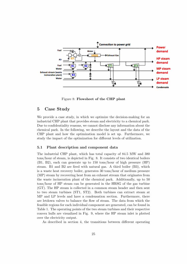
Figure 8: Flowsheet of the CHP plant

5 Case Study

We provide a case study, in which we optimize the decision-making for anindustrial CHP plant that provides steam and electricity to a chemical park.Due to confidentiality reasons, we cannot disclose any information about thechemical park. In the following, we describe the layout and the data of theCHP plant and how the optimization model is set up. Furthermore, westudy the impact of the optimization for different levels of utilization.

5.1 Plant description and component data

The industrial CHP plant, which has total capacity of 84.5 MW and 380tons/hour of steam, is depicted in Fig. 8. It consists of two identical boilers(B1, B2), each can generate up to 150 tons/hour of high pressure (HP)steam. B1 and B2 are fired with natural gas. A third boiler (B3), whichis a waste heat recovery boiler, generates 30 tons/hour of medium pressure(MP) steam by recovering heat from an exhaust stream that originates fromthe waste incineration plant of the chemical park. Additionally, up to 50tons/hour of HP steam can be generated in the HRSG of the gas turbine(GT). The HP steam is collected in a common steam header and then sentto two steam turbines (ST1, ST2). Both turbines can extract steam atMP and LP levels and have a condensation section. Furthermore, thereare letdown valves to balance the flow of steam. The data from which thefeasible regions for each individual component are generated, can be found inTable 1. The operating points of the two steam turbines and their respectiveconvex hulls are visualized in Fig. 9, where the HP steam inlet is plottedover the electricity output.

As described in section 4, the transitions between different operating

25

HP MP LP CON ELB1 75 0 0 0 0

150 0 0 0 0B2 75 0 0 0 0

150 0 0 0 0B3 0 30 0 0 0GT 20 0 0 0 4.9

50 0 0 0 13.6ST1 0 41 31 37 15.8

0 3 0 76 19.00 46 36 58 24.70 29 46 77 31.20 0 88 53 28.90 0 73 64 29.40 0 70 80 34.6

ST2 0 75 75 50 31.90 75 95 30 29.40 95 75 30 27.30 95 95 10 25.20 60 60 55 28.40 60 75 40 26.50 75 60 40 24.90 75 75 25 23.10 60 60 30 19.70 60 75 15 18.00 75 60 15 16.50 60 60 10 13.30 95 75 55 36.3

Table 1: Output data for each individual plant component, from which thefeasible region is created. HP steam: 111 bar, 520◦C; MP steam: 21 bar,320◦C; LP: 4.5 bar, 180◦C. Units: ton/hr for steam, MW for electricity.

26

Figure 9: Operating points of the steam turbines ST1 and ST2 andtheir respective convex hulls.

modes are restricted. In Table 2, the requirements for minimum uptime,the warm and cold startup times are listed. Note that the critical downtimeis 6 hours, after which only a cold startup can be performed. Boiler B3cannot be shutdown, therefore, no values are reported.

Min. uptime Warm startup time Cold startup timeB1 40 1 2B2 24 1 2

B3* - - -GT 1 1 1ST1 2 1 2ST2 4 1 2

Table 2: Requirements for transition times for all components (in hours).

The cost data for the objective function coefficients can be found in Table3. Note that the cost for warm and cold startups only include charges forthe fuel that is consumed during the startup procedure. As noted in section4.9, the additional cost for equipment wear and tear should be included aswell based on historic plant data. Due to the lack of access to this data, wecompare later in this section how shutdown restrictions impact the profit.Based on this comparison, the plant operator can assess whether a shutdownis economically feasible.

Note that due to confidentiality reasons, the reported values for variableand fixed cost coefficients in Table 3 are lumped parameters and include

27

conversion ratios from equations (9) and (11), and the fuel price for naturalgas in equation (37). While the fixed cost coefficient for gas turbine GT isonly assigned if GT is in mode “on”, the fixed cost for boilers B1 and B2are assigned independently of the state of the equipment since the boilersare not shut down completely. Instead, the boilers are always in stand-by ifno HP steam is generated and they are shut down only once per year for amajor revision. Boiler B3 has no cost term since it is a waste heat recoveryboiler that recovers the residual heat from an exhaust stream of the wasteincineration plant of the chemical park, which is provided with no extracharge.

Warm startup [$] Cold startup [$] Variable cost Fixed cost [$/h][$/ton HP]

B1 300 600 24.888 179.2B2 400 800 24.872 182.784

B3* - - - -GT 180 360 29.377 358.4ST1 200 400 - -ST2 230 460 - -

Table 3: Cost table for the individual plant components.

There is a bilateral contract between the industrial CHP plant and theconsumers in the chemical park that defines the product prices for HP, MPand LP steam as well as electricity. The corresponding prices, which areused to calculate the revenue from the chemical park, can be found in Table4. Note that these values are constant over the time horizon of one weeksince they are re-negotiated on a seasonal basis.

HP [$/ton] MP [$/ton] LP [$/ton] EL [$/MWh]Product price 38.40 24.81 9.15 109.16

(internal)

Table 4: Internal product prices based on a contract with the chemical plant(constant over the time horizon).

5.2 Model formulation

The feasible region for each plant component is modeled with equations(2)-(7). Note that the Willans line equation is not included explicitly, asdescribed in section 4. The logic constraint (15) is used to link the modevariables yhc,m for each plant component with the corresponding transitional

variables zhc,m,m� . Constraint (17) enforces that forbidden transitions cannot

be active. Minimum stay restrictions for transitions and uptime (Table 2)

28

are modeled with constraint (18). For sequence dependent transitions, suchas warm and cold startups, constraints (19), (20) and (22) are employed.

The mass balance equations (26)-(28) are included, as well as constraint(29), which enforces that the steam demand is satisfied. The demand forelectricity and steam at different pressure levels is specified on an hourly ba-sis for the time horizon of one week (168 hours). We study different demandscenarios (A-H) that can be found in Table 5, which can be distinguishedby the level of utilization. Note that the demand data assumes a constantdemand profile for the entire week, which is due to the steady-state be-havior of the associated industrial process. The electricity price forecast isassumed to be a typical week in the summer of 2008 based on PJM data(www.pjm.com) and is reported in Table 6. Constraints (30)-(32) are in-cluded to determine the amount of electricity exchanged with the grid. Thecalculation of the profit, which is maximized, is performed with constraints(9), (11) and (35)-(37).

The substation that the plant is connected with, can transmit the max-imum amount of electricity that can be produced within the CHP plant.Therefore, no restriction on the amount of electricity is included. Further-more, no rate-of-change restrictions are included since each component iscapable of ramping from the minimum production level to the maximumproduction level within the given time discretization of one hour. The num-ber of shutdowns is restricted with constraint (34), where the values for SDc

are varied within our case study. The initial state of all components is ’on’.

EL HP MP LP CON % of % ofmax Steam max EL

A-45% 16 10 75 85 0 45% 19%A-45%-B1ST1off 16 10 75 85 0 45% 19%

B-50% 30 30 80 80 0 50% 36%C-61% 40 30 100 100 0 61% 47%D-79% 40 40 120 140 0 79% 47%E-50% 60 30 80 80 0 50% 71%F-76% 60 50 120 120 0 76% 71%G-84% 75 20 100 100 100 84% 89%H-71% 70 10 140 120 0 71% 83%

Table 5: Hourly constant steam (ton/hr) and electricity demand (MWh)for the different cases. The percentages represent the level of utilizationdepending on the maximum steam/electricity output of the CHP plant. Incase A-45%-B1ST1off, boiler B1 and steam turbine ST1 are switched offpermanently due to low capacity utilization.

29

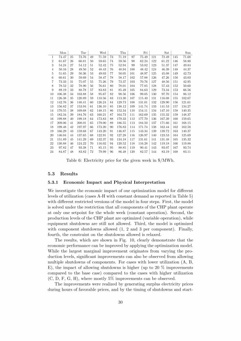
Mon Tue Wed Thu Fri Sat Sun1 74.47 25 73.76 49 71.59 73 71.19 97 75.49 121 72.49 145 71.682 61.67 26 60.81 50 59.65 74 59.56 98 62.24 122 61.22 146 58.803 54.24 27 54.12 51 52.42 75 52.94 99 53.82 123 51.37 147 49.844 50.16 28 49.50 52 48.43 76 48.94 100 48.42 124 46.39 148 44.375 51.65 29 50.36 53 49.03 77 50.05 101 48.97 125 45.08 149 42.736 60.61 30 59.69 54 58.47 78 58.17 102 57.88 126 47.26 150 43.037 73.33 31 75.07 55 75.26 79 73.37 103 70.76 127 48.56 151 42.958 78.52 32 78.90 56 76.61 80 78.01 104 77.85 128 57.43 152 50.609 89.19 33 88.78 57 83.83 81 85.49 105 84.63 129 73.34 153 66.5610 106.38 34 103.88 58 95.67 82 98.56 106 99.05 130 97.70 154 86.1211 126.38 35 120.89 59 110.56 83 113.30 107 115.40 131 116.08 155 102.6712 142.76 36 140.41 60 126.24 84 129.73 108 131.01 132 129.90 156 121.6113 156.82 37 153.94 61 136.10 85 138.12 109 141.74 133 141.53 157 134.2714 170.55 38 169.68 62 148.15 86 152.34 110 154.11 134 147.10 158 140.3515 182.34 39 184.76 63 160.21 87 164.73 111 162.69 135 155.32 159 148.3716 199.88 40 199.18 64 173.83 88 179.33 112 177.70 136 167.39 160 159.6517 209.06 41 208.01 65 179.00 89 186.55 113 184.50 137 171.66 161 168.1518 199.48 42 197.97 66 173.20 90 176.83 114 171.74 138 162.44 162 162.5819 166.29 43 159.68 67 143.20 91 146.87 115 143.34 139 139.72 163 140.3720 146.04 44 137.65 68 122.91 92 127.28 116 126.97 140 123.53 164 125.6921 151.89 45 141.29 69 132.37 93 134.18 117 131.61 141 131.48 165 135.3222 130.88 46 124.22 70 116.02 94 120.52 118 116.28 142 119.18 166 119.8823 97.82 47 93.38 71 85.15 95 88.85 119 90.41 143 93.07 167 93.7424 84.87 48 83.82 72 79.99 96 86.48 120 82.57 144 83.19 168 83.11

Table 6: Electricity price for the given week in $/MWh.

5.3 Results

5.3.1 Economic Impact and Physical Interpretation

We investigate the economic impact of our optimization model for differentlevels of utilization (cases A-H with constant demand as reported in Table 5)with different restricted versions of the model in four steps. First, the modelis solved under the restriction that all components of the CHP plant operateat only one setpoint for the whole week (constant operation). Second, theproduction levels of the CHP plant are optimized (variable operation), whileequipment shutdowns are still not allowed. Third, the model is optimizedwith component shutdowns allowed (1, 2 and 3 per component). Finally,fourth, the constraint on the shutdowns allowed is relaxed.

The results, which are shown in Fig. 10, clearly demonstrate that theeconomic performance can be improved by applying the optimization model.While the largest marginal improvement originates from varying the pro-duction levels, significant improvements can also be observed from allowingmultiple shutdowns of components. For cases with lower utilization (A, B,E), the impact of allowing shutdowns is higher (up to 20 % improvementscompared to the base case) compared to the cases with higher utilization(C, D, F, G, H), where mostly 5% improvements can be observed.

The improvements were realized by generating surplus electricity pricesduring hours of favorable prices, and by the timing of shutdowns and start-

30

Figure 10: Results: Incremental improvements in profit for casesA-H (absolute and relative) due to shutdowns.

31

Figure 11: Case A: Results on component level (in $/MWh forelectricity price, ton/hr for steam and MWh for electricity).

32

Figure 12: Case C: Results on component level (in $/MWh forelectricity price, ton/hr for steam and MWh for electricity).

33

ups of generation assets, while the CHP plant always satisfied the constantsteam and electricity demand of the chemical park. Temporary shutdownsincrease the operational profit since production is stopped when market con-ditions are not in favor to the production of surplus electricity. During thesehours, electricity is even bought from the power grid if the electricity thatis generated by expanding the HP steam according to steam demand doesnot cover the internal electricity demand (see e.g. case C). Additionally, itcan be seen that the permanent shutdown of components (case A-B1ST1off:B1 and ST1 offline) reduces the operational flexibility in such a way thatswings in electricity prices cannot be exploited to the full extent.

For two cases (A and C) with two shutdowns allowed per component, theindividual flows of the components are reported in Fig. 11 and 12. It canbe observed that the HP boilers B1 and B2 adjust their steam productionaccording to the electricity prices. During peak prices, the production is atthe maximum rate. In contrast, if prices are low during the night, the steamproduction is reduced, which is also reflected in the steam flows throughST1 and ST2. The amount of condensate is reduced, which decreases theelectricity production.

If the utilization is low enough, one boiler is even shut down. Note thatduring the same hours one of the steam turbines has to be shut down aswell due to the less amount of HP steam available. If one of the steamturbines goes offline, the extraction flows of the remaining turbine changesaccording to the steam demand such that only small amounts of steamhave to be routed through the letdown valves. The startup proceduresinvolve mostly cold startups, which seem to be more advantageous underthe given electricity prices. The gas turbine GT operates constantly due tothe associated low cost of co-generation of steam and electricity. The MPpressure boiler B3 also operate constantly since it recovers heat from theexhaust stream of the waste incineration plant of the chemical park that isprovided with no cost associated.

5.3.2 Computational Statistics

The resulting optimization model is large, it has as 49,535 variables, ofwhich 8,722 are binary, and 70,009 constraints. Despite the large size, allcases can be solved in less than 2 minutes (except case A with no restrictions,which takes about 9 minutes). The commercial solver CPLEX 12.4.0.1 wasemployed with default settings in GAMS 23.9.1 (Brooke et al., 2012 [73]) ona Intel i7-2600 (3.40 GHz) machine with 8 GB RAM, using a terminationcriterion of 0% optimality gap. The corresponding statistics can be found inTable 7. Note that the requirement of 0% gap ensures that the mathematicaloptimum is reached. If the solution process needs to be sped up, a smalltolerance can be introduced (e.g. 0.1 %).

It can be observed that the optimization problem can be solved faster

34

case constant 0 SD 1 SD 2 SD 3 SD no SDoperation allowed allowed allowed allowed restrictions

A-45% 5 5 12 38 61 526A-45%-B1ST1off 4 4 5 6 6 6

B-50% 5 5 15 62 119 25C-61% 5 5 26 53 40 10D-79% 6 7 8 9 8 8E-50% 5 5 14 54 71 25F-50% 5 5 18 36 31 29G-84% 5 5 9 9 10 10H-71% 5 5 12 11 12 8

Table 7: CPU times in seconds for the investigated cases. SD is an abbre-viation for shutdown, no restrict. means no restrictions for the number ofshutdowns within the week.

if the utilization increases. This behavior is mainly due to the fact that anincreased steam demand implies fewer alternatives for equipment shutdowns,which in turn reduces the solution space.

6 Conclusions

In this paper, we have presented a generalized mode model on a componentbasis for the optimal scheduling of combined heat and power plants undertime-sensitive electricity prices. The model is capable of tracking the statesof the components in terms of operating modes and transitional behavior,and can capture the inherent flexibility of the CHP plant. We applied themodel successfully to a real-world industrial CHP plant. When compared toconstant operation, the optimization model was able to improve the profitup to 5 % for higher utilization cases and up to 20 % for lower utilizationcases, depending on the number of shutdowns allowed. The improvementswere realized by generating surplus electricity prices during hours of favor-able prices, and by the timing of shutdowns and start-ups of generationassets. Therefore, the production profiles for each component adapted tothe swings in electricity prices, while the CHP plant always satisfied thesteam and electricity demand of the chemical park. Despite the large sizeof the resulting MILP model, the problem could be solved within a fewminutes to optimality. The efficient deterministic formulation we reportedcan serve as a basis for the development of models based on the frameworksof stochastic programming (Birge and Louveaux, 2011 [74]) or robust opti-mization (Ben-Tal et al., 2009 [75]), which address uncertainty in electricityprice data originating e.g. from intermittent renewable energy sources.

35

Acknowledgments

We would like to thank the National Science Foundation for financial supportunder grant #1159443. We are also grateful to Joachim Eisenberg for thefruitful discussions on the case study and the data provided.

Nomenclature

Sets

• C (index c): The set of components

• MIX ⊆ C: The set of mixers, that is used to formulate the massbalance for each steam level

• M(c) (index m), abbreviated as Mc: The set of modes, depending oncomponent c

• SM(c,m) (index sm), abbreviated as SMc,m: The set of sub-modes,for mode m depending on component c (e.g. operating regions withdifferent efficiencies for boilers)

• I(c,m) (index i), abbreviated as I: The set of extreme points thatrelate to mode m of component c

• P (index p): The set of products, for the CHP plant it is {HP, MP, LP, CON, EL}

• STL ⊆ P : The set of steam levels, {HP, MP, LP, CON}

• FL (index fl): The set of fuels.

• PIPES(c, p, c�, p�), IN(c, p), OUT (c�, p�): Indicate whether there is asteam pipe connection from component c at steam level p to componentc� at steam level p�.

• H (index h): The set of hours of a week in the operational model

• Seq(c,m,m�,m��): The set of possible transitions for component c frommode m to a production mode m�� with the transitional mode m� inbetween

• MS(c,m,m�): The set of transitions for component c from mode m toanother mode m� with a minimum stay relationship

• DAL(c,m,m�): The set of disallowed transitions from modem to modem� of component c

• StateDep(c,m,m�,m��): Depending on the transition from mode m��

to m, the transition from mode m to m� of component c is restricted

36

• Trajectory(c,m,m�): The set of transitions from mode m to m� ofcomponent c for which a pre-computed trajectory exists

Variables

Binary variables

• yhc,m: Determines whether component c operates in mode m in hour h

• Zh

c,m,m� : Indicates whether there is a transition from mode m to modem� at component c from hour h− 1 to h

Continuous variables

• Prhc,m,g: Production amount of product g in mode m at component cin hour h

• Prhc,g: Total production of product g at component c in hour h

• λh

c,m,i: Variable for the convex combination of slates i to describe the

feasible region of the component c of mode m in hour h

• fuelhc,m: Fuel consumption of component c in mode m

• ∆elh,∆+elh,∆−elh: Difference between produced electricity and elec-tricity demand in hour h

• F h

c,p,c�,p� : Flow from component c at steam level p to component c� atsteam level p� in hour h

• F hcust,p: Steam at steam level p that is sent to the chemical park in

hour h

• F hvent,p: Steam at steam level p that is vented in hour h

• profit: Objective function variable

• cost: Operational cost associated to fuel consumption, startups andshutdowns

Parameters

• αc,m,βc,m, γc,m, �c,m: Fitting parameters related to fuel consumptionfor mode m of component c

• e+h

ext, e−h

ext: External electricity prices in hour h for sales (+) and pur-

chases (-)

• ehint

: Internal electricity prices in hour h

37

• xc,m,i,p: Extreme points of the convex hull of the feasible regions

• Mc,m,p: BigM constant for bounds on production for component c (i.e.max. production of product p in mode m)

• Kmin

c,m,m� : Number of hours component c has to stay in mode m� aftera transition from mode m

• RUc,m,p: Maximum rate of change (up) for product p at component cin mode m

• RDc,m,p: Maximum rate of change (down) for product p at componentc in mode m

• dhp : Hourly demand for product p in hour h. It is the demand for thesteam at different pressure levels and the demand for electricity.

• SFmaxc : Maximum amount of steam generated by supplementary firing

for a gas turbine with HRSG, c ∈ GT .

• crtc: Critical downtime of component c, after which a warm startupis impossible

• TL

c,m,m�,m�� , TU

c,m,m�,m�� : Lower and upper bounds of a time window ac-cording to set StateDep

• F def,h−θ+1c,m,m�,p : Defined output of component c in mode m for product p,

θ hours after a transition from mode m to m�

• SL: Substation limit for the amount of power that is exchanged withthe power grid

• SDc: Number of allowed shutdowns during the time horizon for com-ponent c

• revconst: Constant revenue from internal steam and electricity sales

• fuelpricefl: Fuel price for fuel fl

• steamp: Internal steam price for product p (at steam level STL)

• SUWc: Warm startup cost of component c

• SUCc: Cold startup cost of component c

• SDc: Shutdown cost of component c

38

References

[1] Madlener, R.; Schmid, C., “Combined heat and power generation inliberalised markets and a carbon-constrained world,” GAIA - EcologicalPerspectives for Science and Society, vol. 12, pp. 114–120, 2003.

[2] Kerr, T., “Combined Heat and Power, Evaluating the benefits of greaterglobal investment,” 2008. International Energy Agency report.

[3] Shipley, A.; Hampson, A.; Hedman, B.; Garland, P.; Bautista, P.,“Combined Heat and Power, Effective Energy Solutions for a Sustain-able Future,” 2008. Report by Oak Ridge National Laboratory for theU.S. Department of Energy.

[4] The Press and Information Office of the Federal German Government,“Growth and Responsibility in the World Economy,” 2007. SummitDeclaration (7 June 2007).

[5] The European Parliament, “Directive 2004/8/EC of the European Par-liament and of the Council of 11 February 2004 on the promotion ofcogeneration based on a useful heat demand in the internal energy mar-ket and amending Directive 92/42/EEC,” 2004. 21/02/2004.

[6] German Federal Ministry for the Environment, Nature Conservationand Nuclear Safety, “The Integrated Energy and Climate Programmeof the German Government, background paper as of December 2007,”2007. http://www.bmu.de/english/climate/downloads/doc/40589.php,accessed 04/03/2012.

[7] German Federal Ministry of Justice, “Gesetz fur die Erhaltung, dieModernisierung und den Ausbau der Kraft-Warme-Kopplung (KWKG-Novelle),” 2009. 1. Januar 2009.

[8] The European Commission, eurostat, “Combined heat and power gen-eration, % of gross electricity generation,” 2012.

[9] Federal Reserve, “Industrial Production and Capacity Utilization,”2011. March 2011 release, accessed on 10/21/2011.

[10] German Chemical Industry Association, “Chemical Parks: IndustryLandscaping a la Germany,” Chemical Engineering Progress, vol. 107,no. 10, 2011.

[11] Lewe, T.; Disteldorf, H., “Future challenges for chemical sites, A.T.Kearney study,” 2007.

[12] Lewe, T.; Schroeter, I., “Onsite Service Providers in the Chemical In-dustry, A.T. Kearney study,” 2010.

39

[13] Wassick, J.M., “Enterprise-wide optimization in an integrated chemicalcomplex,” Computers & Chemical Engineering, vol. 33, pp. 1950–1963,2009.

[14] Samad, T.; Kiliccote, S., “Smart Grid Technologies and Applicationsfor the Industrial Sector,” Computers & Chemical Engineering, vol. inpress, 2012.

[15] Todd, D, Caufield, M., Helms, B., Starke M., Kirby B., Kueck, J., “Pro-viding Reliability Services through Demand Response: A PreliminaryEvaluation of the Demand Response Capabilities of Alcoa Inc.,” tech.rep., U.S. Department of Energy, 2009.

[16] Agha, M.; Thery, R.; Hetreux, G.; Hait, A.; Le Lann, J.M., “Integratedproduction and utility system approach for optimizing industrial unitoperations,” Energy, vol. 35, pp. 611–627, 2010.

[17] Christidis, A.; Koch, C.; Pottel, L.; Tsatsaronis G., “The contributionof heat storage to the profitable operation of combined heat and powerplants in liberalized electricity markets,” Energy, vol. 41, pp. 75–82,2012.

[18] Cole, W.J.; Powell, K.M.; Edgar, T.F., “Optimization and Control ofThermal Energy Storage Systems,” Reviews in Chemical Engineering,2012.

[19] Wille-Haussmann B.; Erge T.; Wittwer, C., “Decentralised optimisa-tion of cogeneration in virtual power plants,” Solar Energy, vol. 84,no. 4, pp. 604 – 611, 2010. International Conference CISBAT 2007.

[20] Lund, H.; Andersen, A.N.; Ostergaard, P.A.; Mathiesen, B.V.; Con-nolly, D., “From electricity smart grids to smart energy systems - Amarket operation based approach and understanding,” Energy, vol. 42,pp. 96–102, 2012.

[21] Nishio, M.; Itoh, J.; Shiroko, K.; Umeda, T., “Thermodynamic ap-proach to steam and power system design,” Industrial & EngineeringChemistry Process Design and Development, vol. 19, pp. 306–312, 1980.

[22] Petroulas, T.; Reklaitis, G. V., “Computer-aided synthesis and designof plant utility systems,” AIChE Journal, vol. 30, pp. 69–78, 1984.

[23] Marechal, F.; Kalitventzeff, B., “Process integration: Selection of theoptimal utility system,” Computers & Chemical Engineering, vol. 22,pp. 149–156, 1998.

[24] Papoulias, S.A.; Grossmann, I.E., “A structural optimization apprachin process synthesisI. Utility systems,” Computers & Chemical Engi-neering, vol. 7, pp. 695–706, 1983.

40

[25] Colmenares, T. R.; Seider, W. D., “Synthesis of utility system inte-grated with chemical process,” Industrial & Engineering Chemistry Re-search, vol. 28, pp. 84–93, 1989.

[26] Bruno, J.C.; Fernandez, F.; Castells F.; Grossmann, I.E., “MINLPModel for Optimal Synthesis and Operation of Utility Plants,” Trans-action of the Institution of Chemical Engineers, vol. 76, pp. 246–258,1998.

[27] Iyer, R.; Grossmann, I.E., “Synthesis and operational planning of utilitysystems for multiperiod operation,” Computers & Chemical Engineer-ing, vol. 22, pp. 979–993, 1998.

[28] Willans, P.W., “Economy Trials of a Non-Condensing Steam-Engine:Simple, Compound and Triple. (Including Tables and Plate at Back ofVolume),” Minutes of the Proceedings, vol. 93, pp. 128–188, 1888.

[29] Mavromatis, S.P.; Kokossis, A.C., “Conceptual optimisation of utilitynetworks and operational variations - I. Targets and level optimisation,”Chemical Engineering Science, vol. 53, pp. 1585–1608, 1998.

[30] Varbanov, P.S.; Doyle, S.; Smith, R., “Modelling and Optimization ofUtility Systems,” Chemical Engineering Research and Design, vol. 82,pp. 561–578, 2004.

[31] Aguilar, O.; Perry, S.J.; Kim, J.-K.; Smith, R., “Design and Optimiza-tion of Flexible Utility Systems Subject to Variable Conditions Part1: Modelling Framework,” Chemical Engineering Research and Design,vol. 85, pp. 1136–1148, 2007.

[32] Micheletto, S.R.; Carvalho, M.C.A.; Pinto, J.M., “Operational opti-mization of the utility system of an oil refinery,” Computers & ChemicalEngineering, vol. 32, pp. 170–185, 2008.

[33] Luo, X.; Zhang, B.; Chen, Y.; Mo, S., “Operational planning optimiza-tion of multiple interconnected steam power plants considering environ-mental costs,” Energy, vol. 37, pp. 549–561, 2012.

[34] Seeger, T.; Verstege, J., “Short Term Scheduling in Cogeneration Sys-tems,” Proc. of the 17th Power Industry Computer Application Confer-ence, pp. 106–112, 1991. May 7-10 1991, Baltimore.

[35] Salgado, F.; Pedrero, P., “Short-term operation planning on cogener-ation systems: A survey,” Electric Power Systems Research, vol. 78,pp. 835–848, 2008.

[36] Makkonen S.; Lahdelma, R., “Non-convex power plant modelling in en-ergy optimisation,” European Journal of Operational Research, vol. 171,no. 3, pp. 1113 – 1126, 2006.

41

[37] Tina, G.M.; Passarello, G., “Short-term scheduling of industrial co-generation systems for annual revenue maximisation,” Energy, vol. 42,pp. 46–56, 2012.

[38] Thorin, E; Brand, H.; Weber, C., “Long-term optimization of cogener-ation systems in a competitive market environment,” Applied Energy,vol. 81, pp. 152–169, 2005.

[39] Marshman, D.J.; Chmelyk, T.; Sidhu, M.S.; Gopaluni, R.B.; Dumont,G.A., “Energy optimization in a pulp and paper mill cogeneration fa-cility,” Applied Energy, vol. 87, pp. 3514–3525, 2010.

[40] Dvorak, M.; Havel, P., “Combined heat and power production plan-ning under liberalized market conditions,” Applied Thermal Engineer-ing, vol. in press, 2012.

[41] Ashok, S.; Banerjee, R., “Optimal Operation of Industrial Cogenerationfor Load Management,” IEEE Transactions on Power Systems, vol. 18,pp. 931–937, 2003.

[42] Yusta, J.M.; De Oliveira-De Jesus P.M.; Khodr, H.M., “Optimal energyexchange of an industrial cogeneration in a day-ahead electricity mar-ket,” Electric Power Systems Research, vol. 78, pp. 1764–1772, 2008.

[43] Velasco-Garcia, P.; Varbanov, P.S.; Arellano-Garcia H.; Wozny, G.,“Utility systems operation: Optimisation-based decision making,” Ap-plied Thermal Engineering, vol. 31, pp. 3196–3205, 2011.

[44] Pantelides, C. C., “Unified Frameworks for the Optimal Process Plan-ning and Scheduling,” Proceedings on the Second Conference on Foun-dations of Computer Aided Operations, pp. 253–274, 1994.

[45] Dotzauer, E.; Holmstrom, K.; Ravn, H.F., “Optimal Unit Commitmentand Economic Dispatch of Cogeneration Systems with a Storage,” 13thPSCC Proceedings, pp. 738–744, 1999. Trondheim, Norway, June 1999.

[46] Rong, A.; Hakonen, H..; Lahdelma, R., “A dynamic regrouping basedsequential dynamic programming algorithm for unit commitment ofcombined heat and power systems,” Energy Conversion and Manage-ment, vol. 50, pp. 1108–1115, 2009.

[47] Sandou, G.; Font, S.; Tebbani, S.; Hiretand, A.; Mondon, C., “Shortterm optimization of cogeneration systems considering heat and elec-tricity demands,” 15th Power Systems Computation Conference, Lige,Belgium, 2005.

[48] Padhy, N.P., “Unit Commitment - A Bibliographical Survey,” IEEETransactions on Power Systems, vol. 19, pp. 1196–1205, 2004.

42

[49] Sen, S.; Kothari, D.P., “Optimal thermal generating unit commitment:a review,” International Journal of Electrical Power & Energy Systems,vol. 20, pp. 443–451, 1998.

[50] Hedman, K.W.; O’Neill R.P.; Oren, S.S., “Analyzing Valid Inequalitiesof the Generation Unit Commitment Problem,” Power Systems Con-ference and Exposition, 2009. PSCE ’09. IEEE/PES, pp. 1–6, 2009.

[51] Arroyo, J.M.; Conejo, A.J., “Optimal Response of a Thermal Unit toan Electricity Spot Market,” IEEE Transactions on Power Systems,vol. 15, pp. 1098–1104, 2000.

[52] Carrion, M.; Arroyo, J.M., “A Computationally Efficient Mixed-IntegerLinear Formulation for the Thermal Unit Commitment Problem,”IEEE Transactions on Power Systems, vol. 21, pp. 1371–1378, 2006.

[53] Rajan, D.; Takriti, S., “Minimum Up/Down Polytopes of the UnitCommitment Problem with Start-Up Costs,” tech. rep., IBM ResearchDivision, 2005.

[54] Ostrowski, J; Anjos, M.F.; Vannelli, A., “Tight Mixed Integer LinearProgramming Formulations for the Unit Commitment Problem,” IEEETransactions on Power Systems, vol. 27, pp. 39–46, 2012.

[55] Simoglou, C.K.; Biskas, P.N.; Bakirtzis, A.G., “Optimal Self-Schedulingof a Thermal Producer in Short-Term Electricity Markets by MILP,”IEEE Transactions on Power Systems, vol. 25, pp. 1965–1977, 2010.

[56] Cohen, A.I.; Ostrowski, G., “Scheduling units with multiple operatingmodes in unit commitment,” IEEE Transactions on Power Systems,vol. 11, pp. 497–503, 1996.

[57] Lu, B.; Shahidehpour, M., “Short-Term Scheduling of Combined CycleUnits,” IEEE Transactions on Power Systems, vol. 19, pp. 1616–1625,2004.

[58] Lu, B.; Shahidehpour, M., “Unit Commitment with Flexible Generat-ing Units,” IEEE Transactions on Power Systems, vol. 20, pp. 1022–1034, 2005.

[59] Liu, C.; Shahidehpour, M.; Li, Z.; Fotuhi-Firuzabad, M., “Componentand Mode Models for the Short-Term Scheduling of Combined CycleUnits,” IEEE Transactions on Power Systems, vol. 24, pp. 976–990,2009.

[60] Mitra, S; Grossmann, I. E.; Pinto, J. M.; Arora, N., “Optimal Pro-duction Planning under Time-sensitive Electricity Prices for Continu-ous Power-intensive Processes,” Computers & Chemical Engineering,vol. 38, pp. 171–184, 2012.

43

[61] Balas, E., “Disjunctive Programming and a Hierarchy of Relaxationsfor Discrete Optimization Problems,” SIAM Journal on Algebraic andDiscrete Methods, vol. 6, pp. 466–486, 1985.

[62] Drbal, L.F.; Boston, P.G.; Westra, K.L., Power Plant Engineering.Springer, 1996.

[63] Jacobs, J.A.; Schneider, M., “Cogeneration Application Considera-tions,” 2009. GE Energy report.

[64] Barber, C.B.; Dobkin D.P.; Huhdanpaa, H., “The quickhull algorithmfor convex hulls,” ACM TRANSACTIONS ON MATHEMATICALSOFTWARE, vol. 22, no. 4, pp. 469–483, 1996.

[65] The MathWorks Inc., “MATLAB 7.10.0.499 (R2010a),” 2010.

[66] Christof, T.; Lobel, A., “The PORTA manual page v. 1.4.1,” tech. rep.,ZIB, Berlin, 1997.

[67] Belvaux, G.; Wolsey, L.A., “Modelling Practical Lot-Sizing Problems asMixed-Integer Programs,” Management Science, vol. 47, no. 7, pp. 993–1007, 2001.

[68] Raman, R.; Grossmann, I.E., “Modeling and Computational Tech-niques for Logic Based Integer Programming,” Computers & ChemicalEngineering, vol. 18, p. 563, 1993.

[69] Emberger, H.; Schmid, E., Gobrecht, E., “Fast Cycling Capability forNew Plants and Upgrade Opportunities,” 2005. Siemens Power Gener-ation report.

[70] Lopez-Negrete, R.; DAmato, F.J.; Biegler, L.T.; Kumar, A., “Fastnonlinear model predictive control: Formulation and industrial processapplications,” Computers & Chemical Engineering, vol. in press, 2012.

[71] Lefton, S.A.; Besuner, P.M.; Grimsrud, G.P., “Understand what it re-ally costs to cycle fossil-fired units,” Power, vol. 141, 1997. March/April1997.

[72] Stoppato, A.; Mirandola, A.; Meneghetti, G.; Lo Casto, E., “On the op-eration strategy of steam power plants working at variable load: Tech-nical and economic issues,” Energy, vol. 37, pp. 228–236, 2012.

[73] Brooke, A.; Kendrick, D.; Meeraus, A., “GAMS: A Users Guide, Re-lease 23.9.1,” The Scientific Press, South San Francisco, 2012.

[74] Birge, J.R.; Louveaux, F., Introduction to Stochastic Programming.Springer Series in Operations Research, Springer, 2011.

44

[75] Ben-Tal, A.; El Ghaoui, L.; Nemirovski, A., Robust Optimization.Princeton Series in Applied Mathematics, Princeton University Press,2009.

45