multi-hazard risk analysis: case of a simple offshore
TRANSCRIPT

PB89-145213
NATIONAL CENTER FOR EARTHQUAKEENGINEERING RESEARCH
State University of New York at Buffalo
MULTI-HAZARD RISK ANALYSIS:CASE OF A
SIMPLE OFFSHORE STRUCTURE
by
B.K. Bhartia and E.H. VanmarckeDepartment of Civil Engineering and Operations Research
Princeton UniversityPrinceton, New Jersey 08544
Technical Report NCEER-88-0023
July 21, 1988
This research was conducted at Princeton University and was partially supported by theNational Science Foundation under Grant No. EeE 86-07591.
NOTICEThis report was prepared by Princeton University as a result ofresearch sponsored by the National Center for EarthquakeEngineering Research (NCEER). Neither NCEER, associates ofNCEER, its sponsors, Princeton University or any person actingon their behalf:
a. makes any warranty, express or implied, with respect to theuse of any information, apparatus, method, or processdisclosed in this report or that such use may not infringe uponprivately owned rights; or
b. assumes any liabilities of whatsoever kind with respect to theuse of, or the damage resulting from the use of, any information, apparatus, method or process disclosed in this report.
REPORT DOCUMENTATION 11. REPORT NO.PAGE . NCEER-88-0023
4. Title and SubtitleMulti-Hazard Risk Analysis: Case of a Simple OffshoreStructure
7. Author(s)
B.K. Bhartia and E.H. Vanmarcke9. Performing Organization Name and Address
National Center for Earthquake Engineering ResearchState University of New York at BuffaloRed Jacket QuadrangleBuffalo, NY 14261
12. Sponsoring Organization Name·and Address
15. Supplementary Notes
5. Report DateJuly 21, 1988
6.
8. Performing Organization Rept. No:
10. Project/Task/Work Unit No.
11. Contract(C) or Grant(G) No.
fNCEER-87-3002,(c<'ECE-86-0 7501~)
13. Type of .Report & Period Covered
Technical Report
14.
This research was conducted at Princeton University and was partially supported by theNational Science Foundation under Grant No. ECE-86-07591.
16. Abstract (Limit: 200 words)
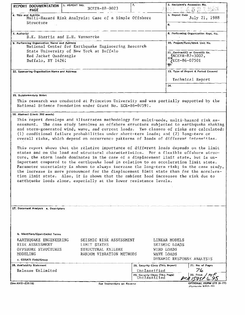
This report develops and illustrates methodology for multi-mode, multi-hazard risk assessment. The case study involves an offshore structure subjected to earthquake shakingand storm-generated wind, wave, and current loads. Two classes of risks are calculated:(1) conditional failure probabilities under short-term loads; and (2) long-term oroverall risks, which depend on occurrenc'~ patterns of loads of different intPDsfties.
This report shows that the relative importance of different loads depends on the limitstates and on the load and structural characteristics. For a flexible offshore structure, the storm loads dominates in the case of a displacement limit state, but is unimportant compared to the earthquake load in relation to an acceleration limit state.Parameter uncertainty is shown to always increase the long-term risk; in the case study,the increase is more pronounced for the displacement limit state than for the acceleration limit state. Also, it is shown that the ambient load increases the risk due toearthquake loads alone, especially at the lower resistance levels.
I--------------------------------.-------------------f17. Document Analysis a. Descriptors
b. Identifiers/Open-Ended Terms
EARTHQUAKE ENGINEERINGRISK ASSESSMENTOFFSHORE STRUCTURESMODELINGc. COSATI Field/Group
SEISMIC RISK ASSESSMENTLIMIT STATESSTRUCTURAL FAILURERANDOM VIBRATION METHODS
LINEAR MODELSSEISMIC LOADSWIND LOADSWAVE LOADSDYNAMIC RESPONSE ANALYSIS
Unclassified20. Security Class (This Page)
Unclassified
18. Availability Statement
Release Unlimited19. Security Class (This Report) I 21. No. of Pages
7-" __I 22. Price / A?~
/)~ 1S!15'"/ b.95'(See ANSI-Z39.18) See Instructions on Reverse OPTIONAL FORM 272 (4 77)
(F'nrrnpf'lv NTI~~«;;"


II[11 11--------
MULTI-HAZARD RISK ANALYSIS:CASE OF A SIMPLE OFFSHORE STRUCTURE
by
B.K. Bhartia1 and E.H. Vanmarcke2
July 21, 1988
Technical Report NCEER-88-0023
NCEER Contract Number NCEER-87-3002
NSF Master Contract Number ECE 86-07591
1 Graduate Student, Dept. of Civil Engineering, Princeton University2 Professor, Dept. of Civil Engineering, Princeton University
NATIONAL CENTER FOR EARTHQUAKE ENGINEERING RESEARCHState University of New York at BuffaloRed Jacket Quadrangle, Buffalo, NY 14261


PREFACE
The National Center for Earthquake Engineering Research (NCEER) is devoted to the expansionand dissemination of knowledge about earthquakes, the improvement of earthquake-resistantdesign, and the implementation of seismic hazard mitigation procedures to minimize loss of livesand property. The emphasis is on structures and lifelines that are found in zones of moderate tohigh seismicity throughout the United States.
NCEER's research is being carried out in an integrated and coordinated manner following astructured program. The current research program comprises four main areas:
• Existing and New Structures• Secondary and Protective Systems• Lifeline Systems• Disaster Research and Planning
This technical report pertains to Program 1, Existing and New Structures, and more specificallyto Reliability Analysis and Risk Assessment.
The long term goal of research in Existing and New Structures is to develop seismic hazardmitigation procedures through rational probabilistic risk assessment for damage or collapse ofstructures, mainly existing buildings, in regions of moderate to high seismicity. This work relieson improved definitions of seismicity and site response, experimental and analytical evaluationsof systems response, and more accurate assessment of risk factors. This technology will beincorporated in expert systems tools and improved code formats for existing and new structures.Methods of retrofit will also be developed. When this work is completed, it should be possible tocharacterize and quantify societal impact of seismic risk in various geographical regions andlarge municipalities. Toward this goal, the program has been divided into five components, asshown in the figure below:
Program Elements:
I Seismicity, Ground Motions Iand Seismic Hazards Estimates I
+I Geoteelmical Studies, Soils Iand Soil-Structure Interaction ~
t
I System Response: ITesting and Analysis I
+ r 1
I Reliability AnalysisI _ ..
and Risk Assessment IExpert Systems
iii
Tasks:Eanhquake Hazards Estimates,GrOlUld Motion Estimates,New Ground Motion Instrumentation,Eanhquake & Ground Motion Data Base.
Site Response Estimates,Large Ground Defonnation Estimates,Soil-Structure Interaction.
Typical Structures and Critical Structural Components:Testing and Analysis;Modem Analytical Tools.
Vulnerability Analysis,Reliability Analysis,Risk Assessment,Code Upgrading.
Architectural and Structural Design,Evaluation of Existing Buildings.

Reliability Analysis and Risk Assessment research constitutes one of the important areas ofExisting and New Structures. Current research addresses, among others, the following issues:
1. Code issues - Development of a probabilistic procedure to determine load and resistance factors. Load Resistance Factor Design (LRFD) includes the investigation ofwind vs. seismic issues, and of estimating design seismic loads for areas of moderateto high seismicity.
2. Response modification factors - Evaluation of RMFs for buildings and bridges whichcombine the effect of shear and bending.
3. Seismic damage - Development of damage estimation procedures which include aglobal and local damage index, and damage control by design; and development ofcomputer codes for identification of the degree of building damage and automateddamage-based design procedures.
4. Seismic reliability analysis of building structures - Development of procedures toevaluate the seismic safety of buildings which includes limit states corresponding toserviceability and collapse.
5. Retrofit procedures and restoration strategies.6. Risk assessment and societal impact.
Research projects concerned with Reliability Analysis and Risk Assessment are carried out toprovide practical tools for engineers to assess seismic risk to structures for the ultimate purposeof mitigating societal impact.
This study focuses on developing and illustrating a methodology for multi-mode, multi-hazardrisk assessment. In this report, both short-term and long-term multi-hazard risk analyses of anoff-shore platform are made. The authors also determine the influence of ambient load on theearthquake safety and the effect ofparameter uncertainty on failure probabilities.
iv

Abstract
This report develops and illustrates methodology for multi-mode, multi-hazard risk as
sessment. The case study involves an offshore structure subjected to earthquake shaking and
storm-generated wind, wave, and current loads. Two classes of risks are calculated: (1) con
ditional failure probabilities under short-term loads; and (2) long-term or overall risks, which
depend on occurrence patterns of loads of different intensities. These risks are calculated
for several combinations of earthquake and storm loads including the ambient load based
on two limit states, both of the first passage type, respectively defined in terms of allowable
displacement and acceleration at the deck level of the structure. Drift or dynamic displace
ment often controls the design of tall structures, while acceleration limit state is useful in
assessing the risk to secondary systems or acceleration-sensitive instruments mounted on
the deck. This report accounts explicitly for two distinct sources of uncertainty in the risk
assessment: one is inherent, essentially irreducible uncertainty, e.g., due to random phasing
of sinusoids in earthquake ground motion, and the other, statistical uncertainty of load and
structural parameters. In the case study, the structure is modeled as a single-degree linear
system with the response analysis performed in the frequency domain using linear random
vibration theory.
This report shows that the relative importance of different loads depends on the limit
states and on the load and structural characteristics. For a flexible offshore structure, the
storm load dominates in the case of a displacement limit state, but is unimportant compared
to the earthquake load in relation to an acceleration limit state. Parameter uncertainty
is shown to always increase the long-term risk; in the case study, the increase is more
pronounced for the displacement limit state than for the acceleration limit state. Also, it is
shown that the ambient load increases the risk due to earthquake loads alone, especially at
the lower resistance levels.
v


ACKNOWLEDGEMENT
This research was supported by the National Science Foundation through the National Center forEarthquake Engineering Research under Agreement NCEER-87-3002 on "Earthquake Engineering: Multi-Hazard Risk Assessment and Management." Any opinions, findings and conclusionsor recommendations are those of the authors and do not necessarily reflect the views of theNational Science Foundation.
vii


SECTION TITLE
TABLE OF CONTENTS
PAGE
1
2
33.13.1.13.1.23.23.2.13.2.23.33.3.13.3.23.3.33.4
4
55.15.1.15.25.2.15.2.25.2.2.15.2.2.25.2.2.35.2.2.45.2.2.55.35.4
66.16.2
INTRODUCTION 1-1
DYNAMIC MODEL 2-1
MODELING OF ENVIRONMENTAL LOADS 3-1Earthquake Load 3-1Seismic Hazard 3-1Spectral Density Function 3-1Wind Load 3-2Statistics of Wind Velocity 3-3Spectral Density Function of Fluctuating Wind Component.. 3-3Wave Load 3-4Wave Height Spectrum 3-4Gravity Waves 3-4Wave Forces and Morison's Formula 3-5Current Load 3-6
PARAMETER UNCERTAINTY .4-1
RESPONSE ANALYSIS 5-1Response to Earthquake Load 5-1Peak Response 5-2Response to Sea-storm Load 5-4Static Response 5-4Dynamic Response 5-5Wind Drag 5-5Wave Drag 5-6Wave Inertia 5-8Total Dynamic Response 5-9Peak Response 5-9Response to Earthquake Load Plus Sea-storm Load 5-10Response to Earthquake Load Plus Ambient Load 5-11
RISK ASSESSMENT 6-1Limit State 6-1Risk Analysis 6-1
IX
SECTION TITLE
TABLE OF CONTENTS (Cont'd)
PAGE
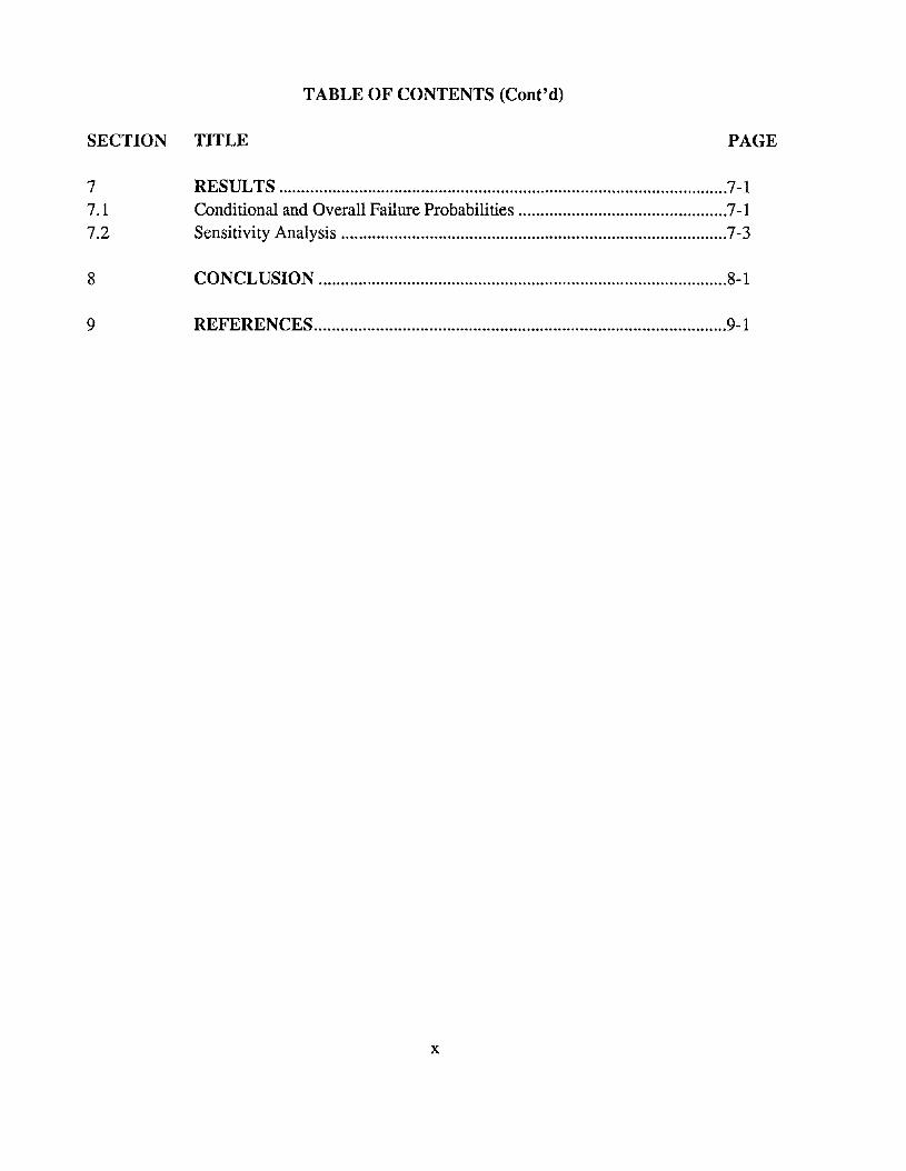
7 RESULTS 7-17.1 Conditional and Overall Failure Probabilities 7-17.2 Sensitivity Analysis 7-3
8 CONCLUSION 8-1
9 REFERENCES 9-1
x
SECTION TITLE
LIST OF ILLUSTRATIONS
PAGE
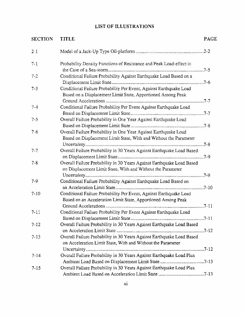
2-1 Model of a Jack-Up Type Oil-platform .2-2
7-1 Probability Density Functions of Resistance and Peak Load-effect inthe Case of a Sea-storm 7-5
7-2 Conditional Failure Probability Against Earthquake Load Based on aDisplacement Limit State 7-6
7-3 Conditional Failure Probability Per Event, Against Earthquake LoadBased on a Displacement Limit State, Apportioned Among PeakGround Accelerations 7-7
7-4 Conditional Failure Probability Per Event Against Earthquake LoadBased on Displacement Limit State 7-7
7-5 Overall Failure Probability in One Year Against Earthquake LoadBased on Displacement Limit State 7-8
7-6 Overall Failure Probability in One Year Against Earthquake LoadBased on Displacement Limit State, With and Without the ParameterUncertainty 7-8
7-7 Overall Failure Probability in 30 Years Against Earthquake Load Basedon Displacement Limit State 7-9
7-8 Overall Failure Probability in 30 Years Against Earthquake Load Basedon Displacement Limit State, With and Without the ParameterUncertainty 7-9
7-9 Conditional Failure Probability Against Earthquake Load Based onan Acceleration Limit State 7-10
7-10 Conditional Failure Probability Per Event, Against Earthquake LoadBased on an Acceleration Limit State, Apportioned Among PeakGround Accelerations 7-11
7-11 Conditional Failure Probability Per Event Against Earthquake LoadBased on Displacement Limit State 7-11
7-12 Overall Failure Probability in 30 Years Against Earthquake Load Basedon Acceleration Limit State 7-12
7-13 Overall Failure Probability in 30 Years Against Earthquake Load Basedon Acceleration Limit State, With and Without the ParameterUncertainty 7-12
7-14 Overall Failure Probability in 30 Years Against Earthquake Load PlusAmbient Load Based on Displacement Limit State 7-13
7-15 Overall Failure Probability in 30 Years Against Earthquake Load PlusAmbient Load Based on Acceleration Limit State 7-13
xi

SECTION TITLE
LIST OF ILLUSTRATIONS (Cont'd)
PAGE
7-16 Conditional Failure Probability Against Sea-storm Load Based ona Displacement Limit State 7-14
7-17 Conditional Failure Probability Per Event, Against Sea-storm LoadBased on a Displacement Limit State, Apportioned Among MeanWind Velocities 7-15
7-18 Conditional Failure Probability Per Event Against Sea-storm LoadBased on Displacement Limit State 7-15
7-19 Overall Failure Probability in 30 Years Against Sea-storm LoadBased on Displacement Limit State 7-16
7-20 Overall Failure Probability in 30 Years Against Sea-storm Load Basedon Displacement Limit State, With and Without the ParameterUncertainty 7-16
7-21 Conditional Failure Probability Against Sea-storm Load Based on anAcceleration Limit State 7-17
7-22 Conditional Failure Probability Per Event, Against Sea-storm LoadBased on an Acceleration Limit State, Apportioned Among MeanWind Velocities 7-18
7-23 Conditional Failure Probability Per Event Against Sea-Storm LoadBased on Displacement Limit State 7-18
7-24 Overall Failure Probability in 30 Years Against Sea-storm Load Basedon Acceleration Limit State 7-19
7-25 Overall Failure Probability in 30 Years Against Sea-storm Load Basedon Acceleration Limit State, With and Without the ParameterUncertainty 7-19
7-26 Overall Failure Probability in 30 Years Against Several Combinationsof Loads Based on Displacement Limit State 7-20
7-27 Overall Failure Probability in 30 Years Against Earthquake Load PlusSea-storm Load Based on Displacement Limit State, With and Withoutthe Parameter Uncertainty 7-20
7-28 Overall Failure Probability in 30 Years Against Several Combinationsof Loads Based on Acceleration Limit State 7-21
7-29 Overall Failure Probability in 30 Years Against Earthquake Load PlusSea-storm Load Based on Acceleration Limit State, With and Withoutthe Parameter Uncertainty 7-21
7-30 Sensitivity of Overall Failure Probability to the Structure's NaturalFrequency Based on Displacement Limit State 7-22
Xli

SECTION TITLE
LIST OF ILLUSTRATIONS (Cont'd)
PAGE
7-31 Sensitivity of Overall Failure Probability to the Structure's DampingRatio Based on Displacement Limit State 7-23
7-32 Sensitivity of Overall Failure Probability to the Structure's NaturalFrequency Based on Acceleration Limit State 7-24
7-33 Sensitivity of Overall Failure Probability to the Structure's DampingRatio Based on Acceleration Limit State 7-25
xiii


TABLE TITLE
LIST OF TABLES
PAGE
2-1
4-1
Dynamic Characteristics and Some Dimensions of the Platform 2-3
Statistics of Uncertain Parameters .4-2
xv


1. Introduction
Multi-hazard risk analysis is concerned with the performance of structures subjected to
multiple random loads, some of which may occur simultaneously. To focus and illustrate the
presentation of the methodology, this report examines a simple model of an offshore structure
subjected to earthquake shaking and sea-storm-generated wind, wave, and current loads.
We compute the integrated risk in the presence of multiple loads and determine the relative
importance of different loads in function of both the structural and load characteristics.
A detailed risk analysis is presented of an offshore oil-platform exposed to four different
combinations of earthquake and sea-storm loads. The load combinations are: (1) earthquake
load alone, (2) earthquake load plus ambient load, (3) sea-storm load alone, and (4) earth
quake load plus sea-storm load. The ambient load of the second load combination arises
due to the ever-present wind over the sea, and is included herein to study its impact on the
earthquake safety.
In general, "failure" is said to occur when the structure or one of its components reaches a
"limit state," i.e., a condition of undesirable behavior or performance. This report calculates
the probabilities of structural failure based on two limit states, defined, respectively, in terms
of relative displacement and (pseudo) acceleration at the deck level of the structure. The
acceleration limit state is relevent in assessing the safety of secondary systems or acceleration
sensitive instruments mounted on the deck. Two classes of failure probabilities are calculated:
(1) conditional failure probabilities under short-term loads; and (2) long-term or overall
failure probabilities, which depend on occurrence patterns of different load intensities.
We account explicitly for two distinct sources of uncertainty in evaluating the probabil
ities of a structural failure. One is inherent, irreducible, uncertainty, e.g., due to random
phasing of sinusoids in earthquake ground motion; and the other is statistical uncertainty of
the load and structural parameters. The latter uncertainty reflects the fact that limited data
are available for the load and structural characteristics to which probability distributions are
assigned instead of deterministic point values. This report seeks to evaluate the effect of this
parameter uncertainty on response statistics and failure probabilities.
The response analysis herein is performed in the frequency domain using linear random
vibration theory, i.e., the equations of motion are linearized based on equivalent linearization
1-1

techniques. Also, the response to both earthquake and sea-storm loads is assumed to be
quasi-stationary during load events of specified durations.
1-2

2. Dynamic Model
For a case study, this report considers a three-legged offshore oil-platform, 80 meters
deep, shown in Fig. 2.1. The structure is modeled as a I-DOF system with only the horizontal
motion. The rotational motion or the vertical drop of the deck are being neglected. The
deck structure for the purpose of the wind load calculation is modeled as an equivalent
rectangular wall normal to the mean wind direction, with height h and width b. The three
legs, tubular in form, are assumed to have full end fixity. Fig. 2.1b shows a dynamic model
of the structure with the dominant mode shape, 'ljJ(z), shown by the dashed line, given as
'ljJ(z) = 1 - cos (~~) , (2.1)
where z is the vertical axis with origin at the sea surface, and l the length of the legs.
Table 2.1 lists the structure's dynamic characteristics and other important dimensions. The
values for modal mass M, stiffness K, and natural frequency W n are calculated based on the
mode shape 'ljJ(z) and the modal damping ratio ( is assumed to be 4.0 %.
To calculate the modal mass, we lump a fraction fm of the virtual mass of the three legs
with the deck mass:
}vI = md + 3[md + ma(l- d)]fm, (2.2)
where md is the deck-mass, ma and m the actual and virtual mass per unit length of a single
leg, respectively, d the water depth, and (l- d) the length of a leg between the still water
level and the bottom of the deck. Factor fm based on the modal analysis [16] is found to be
0.375. The modal stiffness is calculated as
(2.3)
which is the magnitude of the horizontal force at the deck level that produces a unit deflection
at that point. E is the Young's modulus of elasticity and I the rotational moment of inertia.
Thus, the natural frequency of the structure can be written as
W n = .jK/M.
2-1
(2.4)

J0- b .1 x ~Wind
IhDECK r +1,-----,
Load I + I1.. ___ .!
IStill Wate r Level -.- I
II
I
Wave Loao/<z)/
'7zI
d, I
~ 3 EICurrent Load I
I
2EI EI II,,
Mud Lin MAT0
(a) Schematic Diagram (b) Mathematical Model
FIGURE 2-1 Model of a Jack-Up Type Oil Platfonn
2-2

Table 2.1 Dynamic Characteristics and Some Dimensions of the Platform
modal mass (kg) M 5.44x10⁶
modalstiffness(~/m) K 2.67x10⁷
modal natural freq. (rad/sec) (On 2.21
length of legs (m) I 80.0submerged depth (m) d 72.0deck-width (m) b 50.0deck-height (m) h 5.0leg-dia (outer) (m) D 3.7
2-3

3. Modeling of Environmental Loads
Short-term and long-term models for earthquake, wind, wave, and current loads are
presented below. The short-term characterization is concerned with the details of the load
time history during each load event, while the long-term model describes the recurrence
pattern of potentially damaging load events.
3.1 Earthquake Load
Earthquakes at a site occur as a sequence of events which are generally nonstationary
with respect to frequency content and intensity. For the purpose of stochastic analysis, how
ever, motions during each load event are modeled as limited duration segments of stationary
random processes.
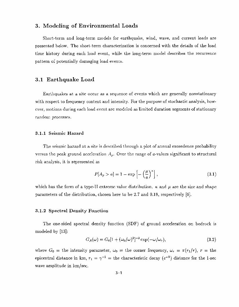
3.1.1 Seismic Hazard
The seismic hazard at a site is described through a plot of annual exceedence probability
versus the peak ground acceleration Ap • Over the range of a-values significant to structural
risk analysis, it is represented as
P[Ap > a] = 1- exp [_ (~)K] , (3.1 )
which has the form of a type-II extreme value distribution. Ii- and J1 are the size and shape
parameters of the distribution, chosen here to be 2.7 and 0.18, respectively [6].
3.1.2 Spectral Density Function
The one-sided spectral density function (SDF) of ground acceleration on bedrock is
modeled by [13]:
(3.2)
where Go = the intensity parameter, Wo = the corner frequency, Wr = 1r(rIfr) , r = the
epicentral distance in km, r1 = ')'-1 = the characteristic decay (e-1) distance for the 1-sec
wave amplitude in km/sec.
3-1

Assuming that Wo is small compared with Wr, which is the case most of the time, an
integration of Eq. 3.2 with respect to W yields the following expression for the variance of
ground acceleration:
O"~ = JGA(w)dw ~ GOwr • (3.3)
Also, the square root of the variance of ground acceleration can be expressed as the peak
ground acceleration Ap divided by a peak factor, assumed here to be 2.75:
Thus, from Eqs. 3.3 and 3.4,Go = (Ap /2.75)2,
Wr
(3.4)
(3.5)
(3.5)
which relates the spectral intensity Go to the peak ground acceleration Ap • The long-term
distribution of Ap is expressed in terms of the curve of site seismic hazard.
The strong motion durations for earthquake load events are uncertain. Their variability
is important especially in the context of nonlinear response. This report, however, treats
only the linear response, and, as a first approximation, assumes a constant duration for each
load event, set equal to 20 sec.
3.2 Wind Load
Structures exposed to gusty wind experience a fluctuating wind load. Assuming a quasi
stationary wind drag coefficient, Cd, the wind load, F(i), may be expressed as
F(i) = ~PaaCdV2(i),
where Pa is the density of air, a the exposed area of the structure normal to the mean wind,
and V(i) the fluctuating wind velocity. Wind load phenomena other than turbulence such as
vortex-shedding, galloping, and flutter are not considered. The wind velocity V(i) is resolved
into a time-independent mean value V and a stationary fluctuating part v(i):
V(i) = tl +v(i). (3.6)
When the fluctuations are small compared with the mean wind, Eq. 3.5 for the wind load
can be linearized:
F(i) ~ ~PaaCd (tl2+2Itllv(i)) ,
3-2
(3.7)
where the first term gives static load, and the second dynamic load in the direction of mean
wind.
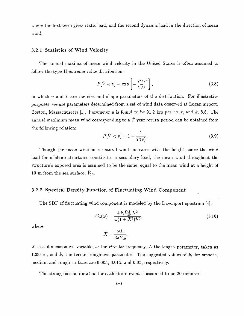
3.2.1 Statistics of Wind Velocity
The annual maxima of mean wind velocity in the United States is often assumed to
follow the type-II extreme value distribution:
(3.8)
in which u and k are the size and shape parameters of the distribution. For illustrative
purposes, we use parameters determined from a set of wind data observed at Logan airport,
Boston, Massachusetts [1]. Parameter u is found to be 91.2 km per hour, and k, 8.8. The
annual maximum mean wind corresponding to a l' year return period can be obtained from
the following relation:-] 1
P[V<v =1-1'(v)' (3.9)
(3.10)
Though the mean wind in a natural wind increases with the height, since the wind
load for offshore structures constitutes a secondary load, the mean wind throughout the
structure's exposed area is assumed to be the same, equal to the mean wind at a height of
10 m from the sea surface, "V;O.
3.2.2 Spectral Density Function of Fluctuating Wind Component
The SDF of fluctuating wind component is modeled by the Davenport spectrum [4]:
4 kr v;.~ X 2
Gv(w) = w(1 +X2)4/3'
where
x= w~ .27rVlO
X is a dimensionless variable, w the circular frequency, L the length parameter, taken as
1200 m, and kr the terrain roughness parameter. The suggested values of kr for smooth,
medium and rough surfaces are 0.005, 0.015, and 0.05, respectively.
The strong motion duration for each storm event is assumed to be 20 minutes.
3-3

(3.11 )
3.3 Wave Load
The wave load on structures is usually described in terms of sea states. A sea state is
an approximately stationary condition described by parameters with long-term fluctuations.
These parameters include the significant wave height, H s , and the mean wave period, Ts •
3.3.1 Wave Height Spectrum
The SDF of wave height in a fully developed sea is modeled in terms of mean wind
velocity, 1110, by the Pierson-Moskowitz spectrum [11]:
ag5 (~g4)GH(W) = -5 exp -11,4 4 '
W lOW
where 9 is the acceleration due to gravity, and a and ~ the spectral parameters. Common
values a = 0.0081 and ~ = 0.74 are adopted.
The significant wave height, H s , and the mean wave period, Ts , are related to the first
two moments of the wave spectrum, and hence uniquely determined by the mean wind VlO •
The mean wind thus provides a useful common base to determine the wind, wave, and
current loads.
3.3.2 Gravity Waves
The kinematics of water particle below the sea surface can be related to the wave height
through a wave theory. Several theories with various degrees of refinements are available,
but stochastic description of wave forces are generally limited to the linear theory of gravity
waves. This theory gives the particle velocity and acceleration, and the dispersion relation
ship as follows:
wH coshkzu(z, t) = - . h kd coswt,
2 sm
. w2 H cosh kz .u(z, t) = -- . h kd smwt,
2 sm
w2 = kg tanh kd,
(3.12)
(3.13)
(3.14)
where u is the particle velocity, it the particle acceleration, k the wave number, and d the
water depth.
3-4

3.3.3 Wave Forces and Morison's Formula
For waves with large wavelengths, the wave load on structures is made up of two compo
nents: a drag force, proportional to the square of the n'ormal component of incident particle
velocity; and an inertia force, associated with the normal component of particle acceleration.
For an oscillating cylinder, the wave force p~r unit lenght, F(t), is given as [10]:
F(t) = ~CdPWa lu(t) - x(t)1 (u(t) - x(t)) +CmPwbu(t) - (Cm - 1)Pwbx(t),2
(3.15)
where Cd is the drag coefficient, Cm the inertia coefficient, Pw the density of water, b the
volume of member, a the projected area of member perpendicular to the motion of fluid,
and x(t) the displacement of the structure. Denoting the relative velocity between water
particles and structure by ur(t), where
ur(t) = u(t) - x(t),
the drag force in Eq. 3.15 can be written as
(3.16)
(3.17)
The nonlinear drag force for a stochastic analysis is linearized by means of equivalent lin
earization techniques [1,5]: the nonlinear term lur(t)lur(t) is replaced with a linear term
dru(t) such that the linearized drag factor, dr, minimizes the mean squared error. Assuming
that ur(t) constitutes a Gaussian process, the equivalent linearization yields
dr = JS/7r O'Ur'
The wave forces, Eq. 3.15, can now be expressed in the following linearized form:
(3.1S)
(3.19)
As evident in Eq. 3.19, the wave force depends on the water particle motion as well as on the
structure's motion. But, since the structure's motion is expected to be small compared with
the water particle motion, the dependence of wave force on the structure's motion is ignored.
It should be noted, however, that this dependence can be easily incorporated by including
the virtual inertia and hydrodynamic drag forces in the equations of motion, and obtaining
the statistics of relative motion through iteration, which is found to converge quickly [9].
3-5

3.4 Current Load
Wind flow over the sea surface generates wind-stressed current in the direction of mean
wind, with the current velocity given as
(3.20)
where uc ( d) is the current velocity at sea surface, and c a proportionality constant, 1-5 %.
The current velocity decreases linearly with depth, dropping to zero at the sea bottom. The
current load on structures is mostly static and predominantly of the drag type.
3-6
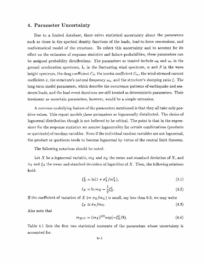
4. Parameter Uncertainty
Due to a limited database, there exists statistical uncertainty about the parameters
such as those in the spectral density functions of the loads, load-to-force conversions, and
mathematical model of the structure. To reflect this uncertainty and to account for its
effect on the estimates of response statistics and failure probabilities, these parameters can
be assigned probability distributions. The parameters so treated include Wo and Wr in the
ground acceleration spectrum, kr in the fluctuating wind spectrum, a and (3 in the wave
height spectrum, the drag coefficient Cd, the inertia coefficient Cm , the wind-stressed current
coefficient c, the structure's natural frequency Wn , and the structure's damping ratio C. The
long-term model parameters, which describe the occurrence patterns of earthquake and sea
storm loads, and the load event durations are still treated as deterministic parameters. Their
treatment as uncertain parameters, however, would be a simple extension.
A common underlying feature of the parameters mentioned is that they all take only pos
itive values. This report models ,these parameters as lognormally distributed. The choice of
lognormal distribution though is not believed to be critical. The point is that in the expres
sions for the response statistics we assume lognormality for certain combinations (products
or quotients) of random variables. Even ifthe individual random variables are not lognormal,
the product or quotients tends to become lognormal by virtue of the central limit theorem.
The following notations should be noted.
Let X be a lognormal variable, mx and (J'X the mean and standard deviation of X, and
AX and ex the mean and standard deviation of logarithm of X. Then, the following relations
hold:
(4.1)
(4.2)
el = In(1 + (J'l /m~),
1 2AX = In mx - -ex.
2
If the coefficient of variation of X (= (J'x /mx) is small, say less than 0.3, we may write
ex ~ (J'X /mx. (4.3)
Also note that
(4.4)
Table 4.1 lists the first two statistical moments of the parameters whose uncertainty is
accounted for.
4-1

The total variability of load or response quantities is made up of the inherent uncer
tainty (R) and the statistical uncertainty (U); the moments of load or response quantities
are subscripted by R or U to indicate the type of uncertainty. Thus, O"X,R denotes the stan
dard deviation of X that arises due to the inherent uncertainty, whereas O"X,U, that due to
the statistical uncertainty.
Table 4.1 Statistics of Uncertain Parameters
Parameter (X)
COo nl2 0.1
cor IOn 0.1
Kr 0.007 0.5
a 0.0081 0.1
~ 0.74 0.1
Cd 0.8 0.1
Cm 1.5 0.25
c 0.03 0.5Tn 2.84 Sec 0.15
~ 0.04 0.25
4-2

5. Response Analysis
The response analysis to dynamic loads is performed in the frequency domain using linear
random vibration theory, with forcing functions assumed to constitute segments of station
ary Gaussian processes. The response processes are also Gaussian. Based on a stationary
response analysis, this section presents the conditional statistics of peak response for load
events involving earthquake only, sea-storm only, earthquake plus sea-storm, and, finally,
earthquake plus ambient vibration. The response statistics presented are always conditional
on the load intensities characterizing each load events.
5.1 Response to Earthquake Load
Let the SDF of ground acceleration at the structure's base be GA(w). If there is a soil
layer in between the structure's base and bedrock, GA(W) can be obtained as
(5.1 )
where GA(w) is the SDF of ground acceleration at the bedrock, given by Eq. 3.2, and Hs(w)
the frequency transfer function of the soil layer. We assume that the structure is founded
on firm ground or bedrock, in which case Hs(w) = 1.0. If the situation varies, Hs(w) may
be used to reflect the effect of local soil [7,13].
Denoting the structure's relative displacement response as X e , the response spectrum
Gxe(w) can be related to the input spectrum GA(w) through a frequency-dependent ampli
fication function, He (w):
(5.2)
where H e (w) is the relative displacement response of the structure to a sinusoidal accelaration
of unit amplitude and frequency w:
(5.3)
Also, the variance of relative displacement, Var [XeJ, can be obtained as the area under its
SDF:
Var[Xe] = 100
GxJw)dw.
5-1
(5.4)

The SDF Gx.(w), however, contains parameters such as W n , (, Wo, Wr, etc. which possess
statistical uncertainty. Var [Xe] thus is seen as a random variable. The 'mean' of Var [XeJ
corresponds to the 'variance' of X e attributed to the inherent uncertainty of the ground
acceleration. Denoted here as OJ.,R' the mean of Var [XeJ is determined by evaluating the
integral (5.4) with the mean values substituted for the uncertain parameters. The 'variance'
of Var [XeJ stems from the statistical uncertainty of the load and structural parameters, and
is calculated herein as follows: A white-noise approximation for Var [Xe ] can be written as
where
(5.5)
I - exp(-wn/wr )
1 - [1 + (wo/wn )2J'
I2 = IHs (wn )12, and al = 1rGo/4 = deterministic quantity. The right hand side of Eq. 5.5
contains parameters and factors which, though uncertain, take only positive values. Invoking
the central limit theorem, Var [XeJ, thus, may be modeled as a lognormal random variable,
regardless of the form of the distributions of the underlying parameters. Now assuming
independence among the terms on the right side of Eq. 5.5, and following the notation of
section four,
e; = Var [log (Var [Xe ])]
= eZ + ge~n +eJl +eJ2'The moments of factors II and 12 are obtained through Taylor series expansion.
(5.6)
For a stationary response, the variance of pseudo acceleration is directly related to that
of the relative displacement:
(5.7)
Thus, the statistics of acceleration response can be obtained in a similar fashion as above.
5.1.1 Peak Response
The peak value of mean-zero Gaussian response process X e can be expressed as
(5.8)
5-2

where Z is a random peak factor. According to Davenport (1964):
vi + 0.557mz = 2ln Vo to + ,.j2ln v(jto
7r 1(Jz = - ,
6 .j2ln v(jto
(5.9)
(5.10)
in which v(j is the mean zero up-crossing rate and to the duration of the stationary response
process. Here, v(j is assumed to be equal to the structure's mean natural frequency (in cycles
per sec) and to is 20 sec.
The right hand side of Eq. 5.8 may be seen as a product of two random variables, the
second of which is random owing to the parameter uncertainty. Making use of the statistics
of Z and Var [XeJ, the first two moments of X pe can be shown as
(5.11 )
(5.12)
(5.13)
Recall that the subscripts Rand U indicate the variability due to the inherent uncertainty
and the statistical uncertainty, respectively. Thus, Eq. 5.13 gives the response variance that
exists solely due to the parameter uncertainty.
For the purpose of risk analysis, let the conditional peak load-effect be denoted as La,
where the subscript a indicates the response dependence on the ground motion intensity.
Then,
(5.14)
(5.15)
Note in Eq. 5.15 that for risk analysis the variances of peak response due to both the inherent
randomness and the parameter uncertainty are added together. Furthermore, the conditional
peak response is assumed to be lognormally distributed, with the mean and variance given
in Eqs. 5.14 and 5.15, respectively. This format is similar to that used in probabilistic risk
assessment in the nuclear industry [3].
5-3

5.2 Response to Sea-storm Load
A sea-storm induces a wind load having both static and dynamic components, a wave
load with only dynamic component, and a current load with only static component. The
response to a sea-storm load thus constitutes a random process with non-zero mean.
5.2.1 Static Response
The total static load, denoted as F, is the sum of drag forces due to wind and current:
The static component of wind drag, FI , is given by Eq. 3.7:
1 -2FI = '2CdPahbVIO,
(5.16)
(5.17)
where F I is conditional on mean wind, Vlo, and contains an uncertain parameter, Cd' Know
ing the statistics of Cd, the first two moments of F I can be found, which for a lognormal Cd
are
(5.18)
(5.19)
The drag force due to current, F2 , integrated over the submerged depth of the legs becomes:
(5.20)
(5.21)
where N is the number of legs, three in this case. On introducing Eq. 3.20, we obtain
1 2 - 2F2 = f,NCdPw Ddc ~o·
The coefficients Cd and c in Eq. 5.21 are taken to be lognormally distributed; assummg
independence and owing to their multiplicative form, the first two moments of F2 are
(5.22)
5-4
(; = ((;2 + 4(;2)1/2<"2,U <"Cd <"c •
If F1 and F2 are assumed independent, the first two moments of F can be written as
2 2 2O"F,U = O"l,U + 0"2,U
The total static displacement, X s , then becomes:
Xs=F/K,
where K is the modal stiffness. Thus,
mxs = mF/K.
O"x s ,u = O"F,U / K.
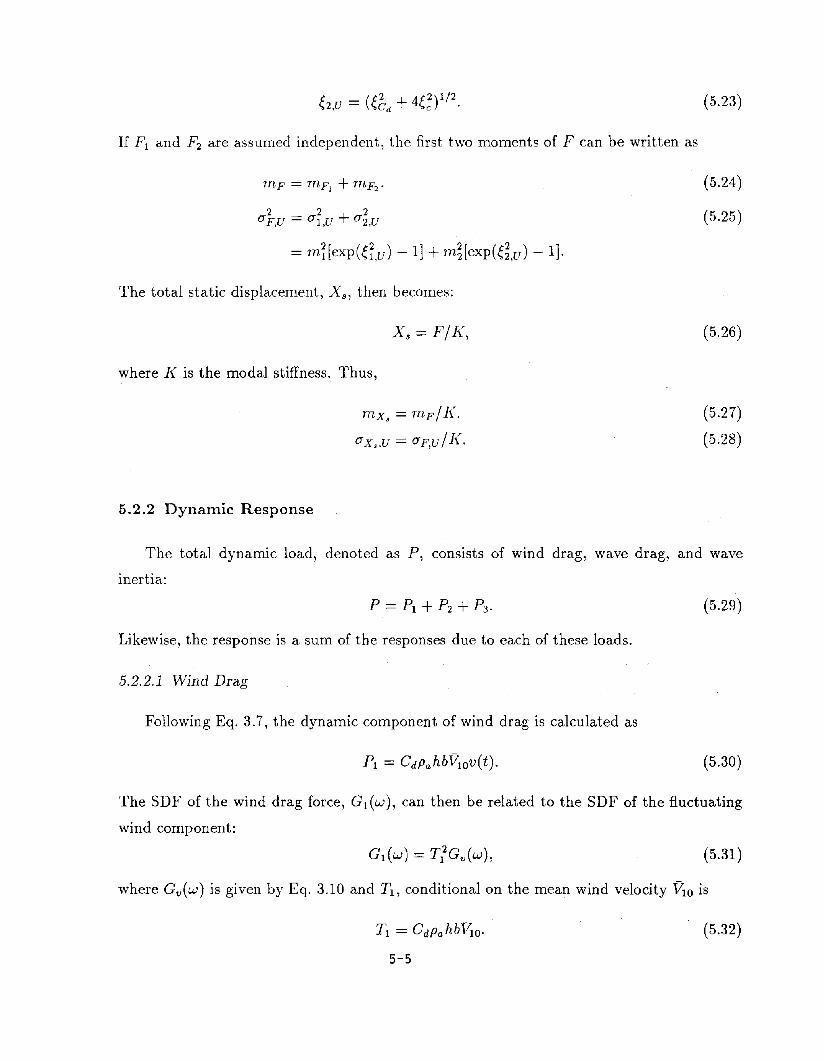
5.2.2 Dynamic Response
(5.23)
(5.24)
(5.25)
(5.26)
The total dynamic load, denoted as P, consists of wind drag, wave drag, and wave
inertia:
(5.29)
Likewise, the response is a sum of the responses due to each of these loads.
5.2.2.1 Wind Drag
Following Eq. 3.7, the dynamic component of wind drag is calculated as
(5.30)
The SDF of the wind drag force, G1 (w), can then be related to the SDF of the fluctuating
wind component:
(5.31)
where Gv(w) is given by Eq. 3.10 and Tl, conditional on the mean wind velocity VlO is
T1 = CdPahbf~o·
5-5
(5.32)
Denoting the structure's relative displacement as XI, its SDF, GX1 (w), is obtained by
(5.33)
where H(w) is the structure's amplification function, i.e., the relative displacement response
to a sinusoidal force with unit amplitude and frequency w:
(5.34)
where M is the modal mass. The variance of Xl can be obtained as the area beneath its
SDF:
Var[XI ] = 100
GX1 (w) dw. (5.35)
Again, since GX1 (w) contains uncertain parameters, Var [Xl] is seen as a random variable.
The mean of Var [Xl], denoted as ui1,R' is obtained by evaluating the integral (5.35) with the
mean values substituted for the uncertain parameters. The variance of Var [Xl] attributed
to the statistical uncertainty in parameters is obtained as follows:
1fVar [Xl] ~ M2( 3 GI(wn ).
4 wn
Upon substituting Eqs. 5.16-17, 3.10, and after some algebraic manipulations:
(5.36)
(5.37)
where
", = (P~b)' C~;13t
is a deterministic quantity. Since the uncertain parameters such as kr , Cd, (, and W n on
the right side of Eq. 5.37 take only positive values, and invoking the central limit theorem,
Var [Xl] may be modeled as a lognormal random variable. Thus,
(5.38)
5.2.2.2 Wave Drag
The sea-waves act on the structure along its height, over which the response, e.g., the
relative displacement, varies. To calculate the modal load, therefore, only a fraction f of the
5-6

wave drag and wave inertia loads are lumped to the total load at the deck level. Assuming a
triangular profile, a conservative choice, for the wave force over the height of the structure,
factor I through modal analysis [16] is found to be 0.55.
Following Eq. 3.20, the drag force due to waves, P2' integrated over the submerged depth
of the legs becomes:
ld 1
P2 = I -NCdPwDlu(z, t)lu(z, t)o 2
ld 1
= I -NCdPwD..;sr; O"u(z)u(z, t) dz.o 2
(5.39)
2 (w cosh kZ) 2 2O"u(z) = "2 sinh kd O"H' (5.40)
where O"H can be obtained from Eq. 3.11 as the root of the area below the wave height
The variance of water particle velocity, O"~(z)' is related to the variance of wave height, O"k,
see Eq. 3.12:
spectrum:
O"H = ~~;.Upon substituting Eqs. 5.40-41 into Eq. 5.39 and carrying out the integration:
(5.41)
p. _ I-1-NC D ~ V120 2 d + (2k)-1 sinh 2kdH .
2 - -/3271" dPw Vf3 2g W sinh2 kd sm wt.
The SDF of wave drag, G2 (w), then is written as
(5.42)
(5.43)
in which GH(w) is given by Eq. 3.11 and T2 , conditional on VIO ' is
To =I-1-NC D ~ V;~ W2d + (2k)-1 sinh 2kd2 -/3271" dPw Vf3 2g sinh2kd . (5.44)
Denoting the relative displacement response to wave drag as X 2 ,
(5.45)
Also, the variance of X 2 is obtained as the area below its SDF:
Var [X2]=100
GX2 (W) dw.
5-7
(5.46)

Again, since GX2 (w) contains uncertain parameters, Var [Xz] is seen as a random variable.
The mean of Var [Xz], denoted as a}2,R, is approximated by evaluating the integral (5.46)
with the mean values substituted for the uncertain parameters, and the variance of Var [Xz]
is obtained as follows:
where
(4.47)
is a deterministic quantity. As argued before, since the uncertain parameters on the right
side of Eq. 5.47 are all positive, Var [Xz] is seen as a lognormal random variable. Thus,
5.2.2.3 ""rave Inertia
e~ = Var [log(Var [Xz])]
= 4e~ +4eb d +a+ e~ + 16e~n +eJ3'
(5.48)
Following Eq 3.20, the inertia force due to waves, P3, integrated over the submerged
depth of the legs becomes:
1rDZldP3 = f NCmpw-- . u(z, t) dz4 0
1rDz WZH 1 ld
= fNCmPw----··-. kdsinwt coshkzdz4 2 smh 0
z= f'!..NCmPwDZwk H sinwt.8 .
The SnF of wave inertia, G3 (w), then is written as
(5.49)
(5.50)
where T3 is1r. W
Z
T3 = fSNCmPwDzT'
5-8
(5.51 )

Denoting the displacement response to wave inertia as X 3 ,
(5.52)
The variance of X3 is equal to the area below its SDF:
Var[X3] = 100
Gxa(w)dw. (5.53)
Here too, GXa(w) contains uncertain parameters and hence Var [X3] is seen as a random
variable. The mean of Var [X3], denoted as U.ka,R' is obtained by evaluating the integral (5.53)
with the mean values substituted for the uncertain parameters, and the variance of Var [X3]
is obtained as follows:
(5.54)
where a3 = deterministic quantity. As we argued before, since the uncertain parameters on
the right side of Eq. 5.54 are all positive, and invoking the central limit theorem, Var [X3]
may be modeled as a lognormal random variable. Thus,
e~ = Var [log(Var [X3 ])]
= e; + 4e~m +eZ + 16e~n + eJ2·
5.2.2.4 Total Dynamic Response
(5.55)
The total dynamic response, denoted as X d , is the sum of responses to wind drag, wave
drag, and wave inertia:
(5.56)
The variance of X d, conditional on the mean wind velocity VIo, is obtained by summing the
variance contributions:
(5.57)
5.2.2.5 Peak Response
The peak value of the combined dynamic response process can be written as
(5.58)
5-9
in which Z is a random peak factor, see Eqs. 5.9-10. Making use of the Eqs. 5.58-59,
statistics of random peak factor Z, and variances of Xl, X 2 , X 3 , we obtain the first two
moments of X p as presented below:
mxp = mz[O"t,Rexp(-~U4) +0"~2,Rexp(-~U4) + 0"~a,Rexp(-~~/4)]1/2.
2 2( 2 2 2)O"Xp,U = O"z O"Xl,R +O"X2,R + O"Xa,R .
O"~p,U = m~{O"~l,R[l - exp(-~U4)] + 0"~2,R[1 - exp(-~U4)]
+ O"t,R[l - exp( -a/4)]}.
(5.59)
(5.60)
(5.61)
For the purpose of risk analysis, a quantity of central interest is the conditional peak of
the total load-effect, denoted here as Lv, which is the sum of the static response and the
peak dynamic response. The subscript v indicates the response dependence on the wind
intensity. Thus,
(5.62)
(5.63)
5.3 Response to Earthquake Load Plus Sea-storm Load
When an earthquake and a sea-storm coincide, the responses to earthquake, wind, wave,
and current loads may be superimposed. The short-duration combined response then has a
static component due to wind and current loads, and a dynamic component due to earth
quake, wind and wave loads. To obtain the peak response, we calculate the peak dynamic
response and add to it the static response. The peak dynamic response is obtained by adding
the individual response variances and then multiplying the root of the total variance by a
random peak factor, dependent on the earthquake's event duration.
Let Y: be the static displacement, X s the static displacement due to wind and current
loads (Eq. 5.26), Yd the dynamic displacement, and ~ the peak dynamic displacement.
Then,
(5.64)
5-10
and
(5.65)
where Xl, X 2 , X 3 , and X e denote the dynamic displacements due to wind drag, wave drag,
wave inertia, and earthquake loads, respectively. Thus,
The first two moments of Yp are given below:
myp = mZ[O"~l,R exp( -eU4) + 0"~2,R exp(-e~/4)
+0"}3,RexP(-eU4)p/2 +O"t,R exp(-e;/4)P/2.
2 2( 2 2 2 2)0"X U = O"Z 0"X R + O"X2R + 0"X3 R + 0"X R .p, 1, , , e,
O"}p,U = m~{O"t,R[l - exp( -eU4)] +0"}2,R[1 - exp( -eU4)]
+O"t,R[l - exp( -eV4)] +O"t,R[l - exp( -e;/4)]}.
(5.66)
(5.67)
(5.68)
(5.69)
Let the conditional total peak response be denoted as L av , where the subscript indicates
the response dependence on the earthquake and sea-storm intensities, A and V, respectively.
We may write
(5.70)
(5.71)
5.4 Response to Earthquake Load Plus Ambient Load
When shaken by an earthquake offshore structures in addition experience the ambient
wind, wave, and current loads that arise from the ever-present wind over the sea. Due to
the ambient load the structure's response developes a bias, e.g., the displacement response
developes a non-zero mean in the direction of the mean wind (assuming the same direction
for the sea currents).
This load combination is a special case of the previous one, where we now specify a
nominal constant value for the wind intensity V. Denoting the total peak response as La.. ,
where the subscript a* indicates the response dependence on the earthquake intensity, A, and
a nominal sea-storm intensity, the first two moments of La.. are obtained from Eqs. 70-71,
by substituting a nominal constant value for the mean wind.
5-11


6. Risk Assessment
6.1 Limit State
An important ingredient of risk analysis is the identification of limit states, i.e., states of
undesirable structural behavior. The probabilities of structural failure are calculated with
reference to different limit states. This report considers two limit states, both of the first pas
sage type, defined, respectively, in terms of relative displacement and (pseudo) acceleration
at the deck level of the structure. Since the structure is modeled as a linear I-DOF system,
either of the two limit states can represent the allowable force, however, both cover some
distinct aspects of structural behavior: the displacement limit state may also represent ser
viceability, i.e., the allowable displacement at the deck level; and, the acceleration limit state
is pertinent to assessing the safety of secondary systems or acceleration-sensitive instruments
mounted on the deck. The allowable limits, i.e., the resistances, are often random; they are
modeled herein as lognormally distributed random variables, but with constant coefficient
of variation, set at 0.25. The structural performance is assessed with several values for the
mean resistance.
6.2 Risk Analysis
An offshore structure during its design life is subjected to intermittent loads due to
earthquakes and sea-storms. The intensities of these loads, their occurrence patterns, the
load parameters, the dynamic characteristics of the structure, and the structural resistance
are all uncertain. Some of these, for example, the intensities and the occurrence patterns
of the loads are inherently random, while others are statistically uncertain. To quantify the
performance of the structure in this uncertain environment involves calculating the proba
bilities of structural failure during a prescribed period of time (O-t). The following format
has been adopted herein to calculate the failure probabilities.
First we calculate the "conditional failure probability," Pflq,r, defined as the probability
of structural failure given that a load event of intensity q occurs and that the structural
resistance is r. The parameter q for a coincidental load event is a vector, i.e., q = av for the
event of simultaneous occurrence of earthquake and sea-storm. Also, the structural resistance
6-1

r, in general, is statistically uncertain and may degrade with time. The failure probability,
therefore, needs to be convolved with the distribution of R, the uncertain resistance, at
an appropriate stage of risk analysis. Recall that this report treats various other load and
structural parameters as random variables too, which, in effect, renders the response statistics
to be uncertain. For example, the stationary response variance to the earthquake load was
seen in section five to be random and lognormally distributed, with the variability attributed
to the uncertain parameters. There are several ways one can account for this additional
uncertainty in a risk analysis. This report adopts an approach whereby we calculate the
statistics of the peak load-effect, L q , due to the individual and coincidental load events, and
assume that the peak load-effects are lognormally distributed. The mean and the variance of
L q include the effect of uncertainty in the load and structural parameters. In other approach,
for example, the barrier crossing approach [12,14], one may first calculate the conditional
failure probability, Pflq,r,u, where the additional subscript u indicates the response dependence
on a vector of uncertain parametrs, U, and then from it obtain Pflq,r by convolution.
The conditional failure probability, Pflq,Tl for a lognormal conditional load-effect, Lq, is
calculated as
where
Pflq,r = P[Lq > r]
= <1>( -(3q),
13 - _ In J.lq
q - Vln(1 +Vlq
) ,
J.lq = r/mLqV1 +Vlq,
(6.1 )
VLq = the coefficient of variation of Lq, and <1>(.) = the probability function of a standard nor
mal variable. The index (3q is a conditional reliability index directly related to the conditional
failure probability.
The "conditional failure probability per event," Pf/rl given that an event occurs (the
event intensity is now random) and that the structural resistance is r, is then obtained by
convolving Pflq,r with the distribution of the intensity parameter Q:
Pflr = JPflq,r fQ(q) dq.
6-2
(6.2)

In a long-term risk analysis, we consider only those load events that exceed certain
thresholds on the load-event-intensities. This report sets 20 gal for the peak ground acceler
ation of earthquake load events and 36 km per hour for the mean wind velocity of sea-storm
load events, respectively, as the thresholds. The criterion for adopting these values is that
the contribution of the load events with lower intensities to the failure probabilities per event
are negligible. Setting the thresholds also gives the mean yearly event-occurrence rates, see
Eq. 3.9, and the normalized intensity distribution functions to be used in the convolution
in Eq. 6.2. The mean event-occurrence rates for earthquake and sea-storm are obtained
through Eqs. 3.1, 3.8, and 3.9 as 0.5 per year and 1.0 per year, respectively.
The long-term or "overall" probability of structural failure due to a single intermittent
load say in t years of service life is calculated as
(6.3)
where N is the total number of load events in t years. If Pllr is small and the events occur
as points in a Poisson process, Eq. (6.3) can be rewritten as
PI,t = 1- Jexp(-AtPllr) fR(r) dr,
where A is the mean yearly event-occurrence rate of the load.
(6.4)
In the case of two independent, intermittent loads, there exist three kinds of load events:
two individual load events and one coincidental load event. The overall failure probability,
assuming Poisson arrivals for the the load events, then can be calculated as [15]:
PI,t = 1- Jexp [-(V1Pllr + V2P21r + V12P12Ir)t] fR(r)dr, (6.5)
where Pilr stands for 'Pllr' for the individual events of the ith load, P121r that for the co
incidental load, Vi is the mean yearly event-occurrence rate of load i, and V12 that of the
coincidental load. For two independent loads with Poisson arrival:
Vi = Ai[1 - L Aj(to1 + t02 )],i¥-j
V12 = A1 A2(tQ1 + to2 ),
in which tOi is the event duration of load i.
6-3
(6.6)

If the failure probabilities Pilr and P12lr are very small, if the load events are rare, or if the
variability in the structural resistance is small, one may convolve Pilr and P121r individually
with the distribution of the uncertain resistance, R, to obtain the unconditional failure
probabilities per events of the individual and coincidental loads, respectively:
Pi = JPilr fR(r) dr;
P12 = JP12lr fR(r) dr.
Vie may then rewrite Eqs. 6.4 and 6.5, respectively, as
PI,t = 1 - exp( -At PI),
and
(6.7)
(6.4a)
(6.5a)
However, doing so amounts to assuming that the structural resistance from event to event is
independent, and also ignores the fact that the combined load-effect and not the individual
load-effect see the variability in the resistance. As a result, Eqs. 6.4a and 6.5a would always
yield conservative estimates for the long-term failure probabilities. In the next section, we
show several numerical results to substantiate this point.
The format of long-term risk assessment through Eqs. 6.4 and 6.5 is also easily amenable
to include any degradation in the structural resistance over time.
The conditional failure probability per event against coincidental load, i.e., that due to
the simultaneous occurrence of earthquake and sea-storm loads, is obtained by convolution:
P12!r = JJP12!av,r dFA(a) dFv(v). (6.8)
However, note that the event duration for an earthquake is only 20 sec as opposed to the
assumed 20 minutes for a sea-storm alone. Thus, a coincidental load is invariably accom
panied by a sea-storm load acting separately. Therefore, the conditional failure probability
per event of a coincidental load, P12jr, is the failure probability of a system with two failure
events in series:
P121r = 1 - (1 - P121r)(1 - P2Ir),
where P21r is the conditional failure probability per event against sea-storm loads.
6-4
(6.9)

7. Results
7.1 Conditional and Overall Failure Probabilities
In Fig. 7.1, we demonstrate the profound effect parameter uncertainty has on the response
statistics. Shown in the figure are the probability density functions of resistance and peak
response to a sea-storm load. The mean wind velocity of the sea-storm is 140 km/hr and the
mean and the coefficient of variation (COV) of the resistance are 25 cm and 0.25, respectively.
The figure shows that the presence of parameter uncertainty leads to a steep increase in the
COY of the peak response: to 0.37 from 0.04; but a slight decrease in the mean: to 15 cm
from 16 cm. A decrease in the mean occurs due to the lognormality of the stationary response
variance, as shown in section five. It is interesting to note that the simultaneous occurrence
of an increase in the COY of the peak response while a decrease in its mean may steer the
conditional failure probability either way: an increase, or may be a decrease, depending on
the load intensity and other parameters.
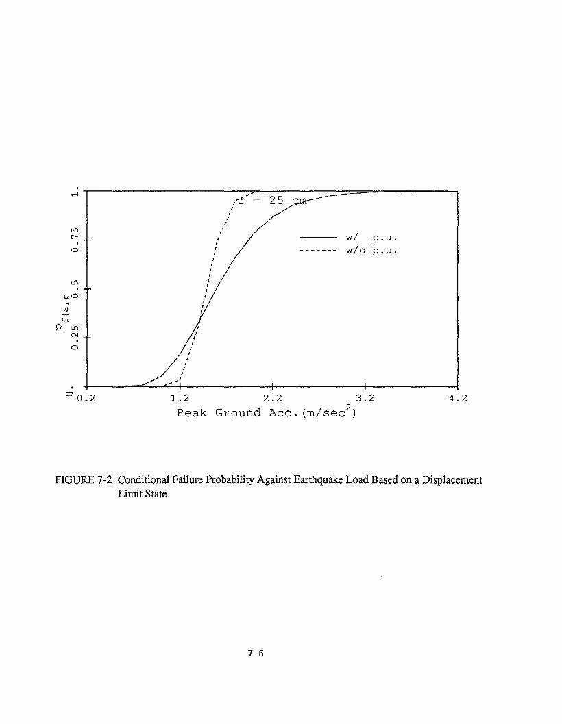
Figs. 7.2-7.8 show the probabilities of structural failure against earthquake load based
on displacement limit state. In Fig. 7.2, we plot the conditional failure probability versus the
peak ground acceleration when the allowable displacement at the deck level of the structure is
25 cm, both with and without the parameter uncertainty. Interestingly enough, the presence
of parameter uncertainty leads to an increase in the conditional failure probability only when
the peak ground acceleration is less than around 1.6 m/sec2 , a decrease otherwise. It indicates
that if the contribution of events with peak ground acceleration less than 1.6 m/sec2 outweigh
the contribution of events with higher intensity to the conditional failure probability per
event, the presence of parameter uncertainty will lead to an increase in the overall failure
probability. In Fig. 7.3, we apportion the conditional failure probability per event, Pljr,
among the contributing peak ground accelerations. We see that most of the contribution to
Pllr comes from earthquake-events with intensities around 1.5 m/sec2• In Fig. 7.4, we plot Pllr
versus resistance with and without the parameter uncertainty. The parameter uncertainty is
seen to always increase the failure probability per event, though the increase is pronounced
only at lower resistance levels. Fig. 7.5 shows the yearly failure probability versus the mean
resistance calculated in two different ways. Recall that the structural resistance possesses
statistical uncertainty, and at what stage of risk analysis the failure probability is convolved
7-1
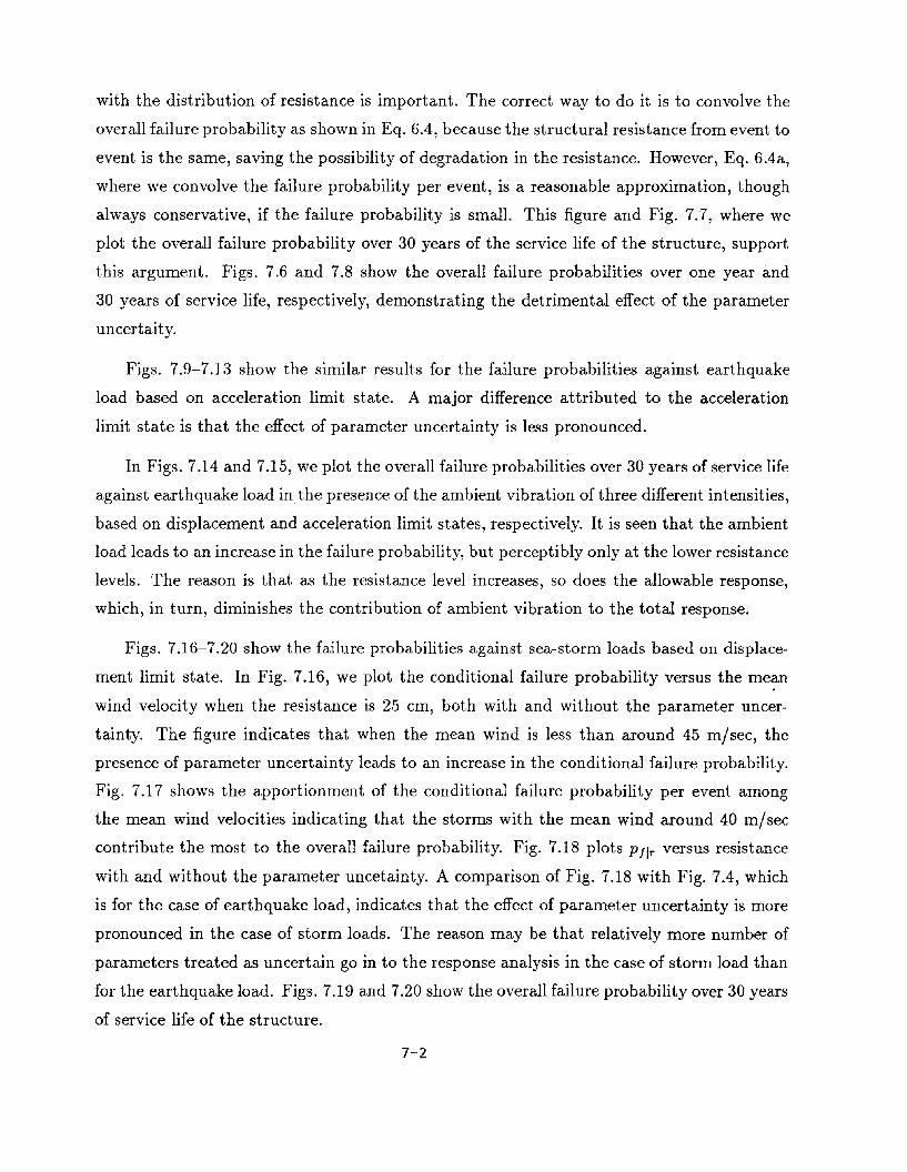
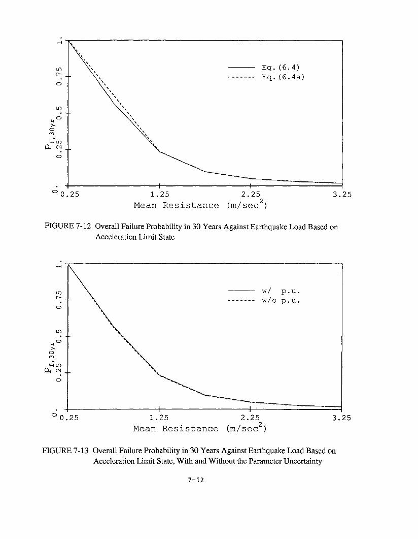
with the distribution of resistance is important. The correct way to do it is to convolve the
overall failure probability as shown in Eq. 6.4, because the structural resistance from event to
event is the same, saving the possibility of degradation in the resistance. However, Eq. 6.4a,
where we convolve the failure probability per event, is a reasonable approximation, though
always conservative, if the failure probability is small. This figure and Fig. 7.7, where we
plot the overall failure probability over 30 years of the service life of the structure, support
this argument. Figs. 7.6 and 7.8 show the overall failure probabilities over one year and
30 years of service life, respectively, demonstrating the detrimental effect of the parameter
uncertaity.
Figs. 7.9-7.13 show the similar results for the failure probabilities against earthquake
load based on acceleration limit state. A major difference attributed to the acceleration
limit state is that the effect of parameter uncertainty is less pronounced.
In Figs. 7.14 and 7.15, we plot the overall failure probabilities over 30 years of service life
against earthquake load in the presence of the ambient vibration of three different intensities,
based on displacement and acceleration limit states, respectively. It is seen that the ambient
load leads to an increase in the failure probability, but perceptibly only at "the lower resistance
levels. The reason is that as the resistance level increases, so does the allowable response,
which, in turn, diminishes the contribution of ambient vibration to the total response.
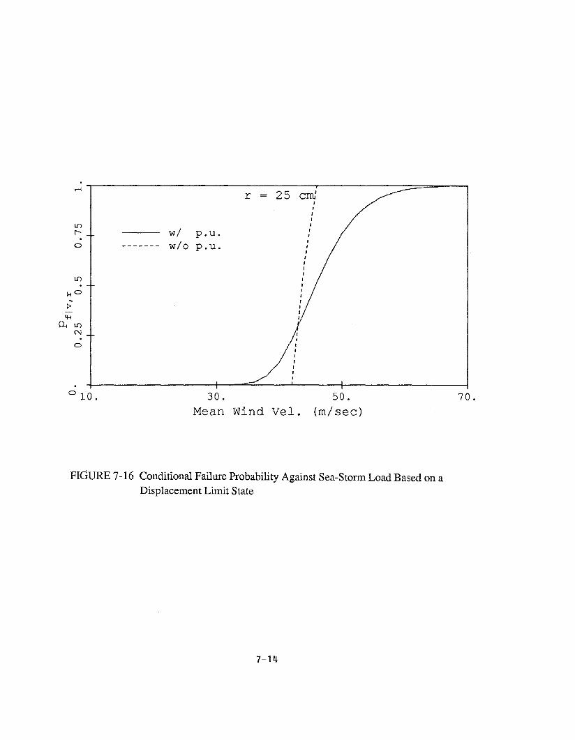
Figs. 7.16-7.20 show the failure probabilities against sea-storm loads based on displace
ment limit state. In Fig. 7.16, we plot the conditional failure probability versus the mean
wind velocity when the resistance is 25 cm, both with and without the parameter uncer
tainty. The figure indicates that when the mean wind is less than around 45 m/sec, the
presence of parameter uncertainty leads to an increase in the conditional failure probability.
Fig. 7.17 shows the apportionment of the conditional failure probability per event among
the mean wind velocities indicating that the storms with the mean wind around 40 m/sec
contribute the most to the overall failure probability. Fig. 7.18 plots P!lr versus resistance
with and without the parameter uncetainty. A comparison of Fig. 7.18 with Fig. 7.4, which
is for the case of earthquake load, indicates that the effect of parameter uncertainty is more
pronounced in the case of storm loads. The reason may be that relatively more number of
parameters treated as uncertain go in to the response analysis in the case of storm load than
for the earthquake load. Figs. 7.19 and 7.20 show the overall failure probability over 30 years
of service life of the structure.
7-2

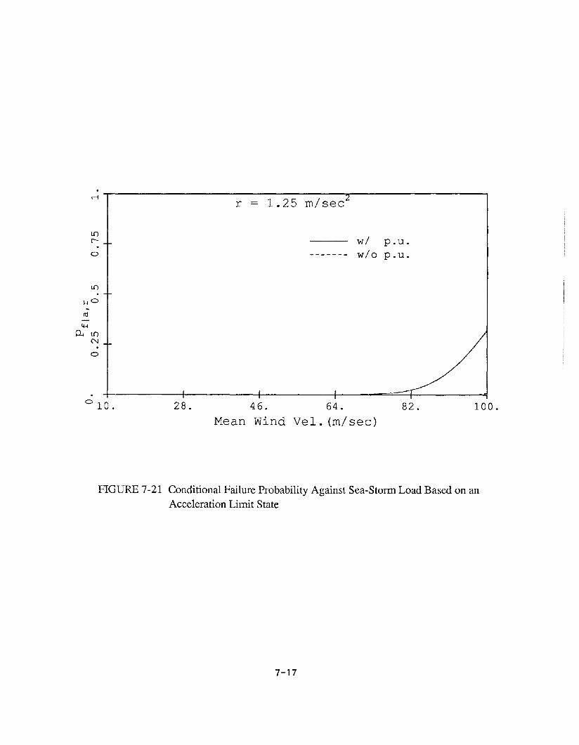
Figs. 7.21 to 7.25 show the failure probabilities against sea-storm load based on accelera
tion limit state. The results are dramatic. Both conditional and overall failure probabilities
are seen to be exceedingly small. To put the results in perspective, recall that the mean nat
ural period of the structure is 2.84 sec, far from the 25 sec period for the predominant wave.
As a result, although storm loads induce large displacements, the acceleration response is
small. This result is beneficial in that that acceleration-sensitive instruments or secondary
systems mounted on the deck are not at risk during sea-storms; though, they might get
blown off the deck.
In Fig. 7.26, based on displacement limit state, we plot the overall failure probabilities
over 30 years for four different combinations of environmental loads, namely, earthquake load
alone; earthquake load plus ambient load; sea-storm load alone; and earthquake load plus sea
storm load, with and without the load-coincidence. It is seen that the storm load governs the
design, and the effect of coincidental load on the overall risk is negligible. Fig. 7.27 shows the
30-year-overall failure probability based on displacement limit state against both earthquake
and storm loads acting on the structure, with and without the parameter uncertainty. The
parameter uncertainty is seen to substantially increase the failure probability. Figs. 7.28
7.29 show the similar results in the case of acceleration limit state indicating that in this
case the earthquake load governs the design, and the effect of parameter uncertainty is less
important.
7.2 Sensitivity Analysis
The sensitivity of 30-year-overall failure probability against both earthquake and sea
storm loads acting on the structure has been investigated with reference to the mean and the
coefficient of variation of the structure's natural frequency and the damping ratio. Figs. 7.30
and 7.31 show the results for the case of displacement limit state, while Figs. 7.32 and 7.33
for the case of acceleration limit state.
In Fig. 7.30a, we plot the 30-year-overall failure probability for three different values of
mean natural frequency of the structure. As the structure becomes stiffer, due the displace
ment type limit state, the failure probability decreases. Fig. 7.30b shows the sensitivity of the
failure probability to the variability in the natural frequency. It is apparent that the failure
7-3

probabilities are very sensitive to the variability in the natural frequency. Fig. 7.31 shows the
sensitivity of 30-year-overall failure probability to the mean and the COV of the damping
ratio. It is seen that the overall risk increases with the decrease in the mean damping and
an increase in its variability.
In Fig. 7.32, based on acceleration limit state, we plot 30-year-overall failure probability
for three different values of the mean natural frequency and three different values of its COV.
The overall risk increases as the structure becomes stiffer, because of the acceleration type
limit state. The overall risk in this case is less sensitive to the variability in the natural
frequency. Fig. 7.33 shows similar result for the structure's damping ratio.
7-4

0...--------------------------------,rl
load-effect wlo p.u.load-effect wi p.u.resistance
lI)
r->t+J-r!(f)
C<VQ
>t+J lI).r!.-I-r!,.QcD
,.Q0~
P-4L.()
N
,,..----- ...,,,,,,,
/
---0 0 • 10. 20.
Displacement30.
(meter)40. 50.
xlO-2
FIGURE 7-1 Probability Density Functions of Resistance and Peak Load-Effect in the Case of aSea-Storm
7-5
wi p.u.------- w/o p.u.
1.1)
o
..--l I-------------::..:-:--- -----=::::::::===~-----....,
,'f =,,,,,,,IIII
IIIIII
I,II
1.1)
r-
o
..ro4-l
0-.1.1)N
1.2 2.2 3.2
Peak Ground Ace. (m/ sec2
)
4.2
FIGURE 7-2 Conditional Failure Probability Against Earthquake Load Based on a DisplacementLimit State
7-6

(V)
IoriX
r - 25 cm
H
~
O-t
4--l <:l'
0
.j..J
~(1)
8~0 N
.r!.j..JH0O-tO-t~
00. 2. 4. 6.Peak Ground Acc. (m/ sec
2)
8.
(V)
IoriX U} ,..- ---,
.-i
FIGURE 7-3 Conditional Failure Probability Per Event, Against Earthquake Load Based on aDisplacement Limit State, Apportioned Among Peak Ground Accelerations
o.-i
,,,,,,,,,,,,,,,,,.. .. .. .. .. .. ..
wi p.u.------- w/o p.u.
020. 30.
Resistance40.
(cm)50.
FIGURE 7-4 Conditional Failure Probability Per Event Against Earthquake Load Based onDisplacement Limit State
7-7

(Y)
IC)
rl:x: 0 .,-- --,
rl
Lf)Eq. (6.4)
------- Eq.(6.4a)
N
0 20 . 30.Mean Resistance
40.(em)
50.
FIGURE 7-5 Overall Failure Probability in One Year Against Earthquake Load Based onDisplacement Limit State
(Y)
IC)
rl:x: 0 .,-- --,
rl
Lf)wi p.u.
------- w/o p.u.
N
----
0 20 . 30.
Mean Resistance40.
(em)50.
FIGURE 7-6 Overall Failure Probability in One Year Against Earthquake Load Based onDisplacement Limit State, With and Without the Parameter Uncertainty
7-8

NIorlX 0 ~ ....,
(V)
oN
,, ,,,,, ,, ,,, ,,,'" , , ,
Eq. (6.4)------- Eq. (6.4a)
0 20 . 30. 40.
Mean Resistance (ern)50.
FIGURE 7-7 Overall Failure Probability in 30 Years Against Earthquake Load Based onDisplacement Limit State
NIorl
X 0-,----------------------------------,(V)
wi p.u.------- wlo p.u.
oN
, , , , , , , , , ,, , , ,"
---- ------
0 20 . 30. 40.
Mean Resistance (ern)50.
FIGURE 7-8 Overall Failure Probability in 30 Years Against Earthquake Load Based onDisplacement Limit State, With and Without the Parameter Uncertainty
7-9

wi p.u.------- w/o p.u.o
o
rl,---------------=c-=---===-------.,.,----------------,/r 1 • 25m/ sec~
~
III
II
I,I,,
I,,,II,1>-1 0
0 0 . 2 1.2 2.2 3.2Peak Ground Ace. (m/ sec
2)
4.2
FIGURE 7-9 Conditional Failure Probability Against Earthquake Load Based on anAcceleration Limit State
7-10

NI0rl:x: N
rl
H
~
~ro
4--l 0
0
.wc([)
8c '<l'
00-rl
.wlY0~
~
0 0 •
r 1.25 m/sec
2. 4. 6.
Peak Ground Acc. (m/ sec2)
8.
FIGURE 7-10 Conditional Failure Probability Per Event, Against Earthquake Load Based on anAcceleration Limit State, Apportioned Among Peak Ground Accelerations
o
o
\\
\\
\\\
\\\\
\\\\
\\
\\
\\
\\
\\ ,
wi p.u.------- w/o p.u.
1.25
Resistance2.25
2(m/ sec )3.25
FIGURE 7-11 Conditional Failure Probability Per Event Against Earthquake Load Based onDisplacement Limit State
7-11
lI)
L-
o
lI)
..4-llI)
p"!N.o
,,,,,,,,,,,,,,,,,,,,,,,\ ,,
\\ ,,
1. 25Mean Resistance
Eq. (6.4)------- Eq. (6.4a)
2.252(m/ sec )
3.25
FIGURE 7-12 Overall Failure Probability in 30 Years Against Earthquake Load Based onAcceleration Limit State
lI)
L-
a
lI).H
O
>to(Y')..4-llI)
p"!N
o
a 0.25
wi p.u.w/o p.u.
1.25 2.25Mean Resistance (m/sec2
)
3.25
FIGURE 7-13 Overall Failure Probability in 30 Years Against Earthquake Load Based onAcceleration Limit State, With and Without the Parameter Uncertainty
7-12

NI0rlX 0
(Y)
V = 0 km/hr------- V 30 km/hr- - -- v = 45 km/hr
0 - - - 60 km/hrN
020. 30.Mean Resistance
40.(cm)
50.
FIGURE 7-14 Overall Failure Probability in 30 Years Against Earthquake Load Plus AmbientLoad Based on Displacement Limit State
.-l
V = 0 km/hrL1)r- v 30 km/hr0 v 45 km/hr
v = 60 km/hrL1).
1-10
>.0(V)..4-!L1)
0-4 N
0
1.25 2.25Mean Resistance (m/sec2
)
3.25
FIGURE 7-15 Overall Failure Probability in 30 Years Against Earthquake Load Plus AmbientLoad Based on Acceleration Limit State
7-13
L1)c-
o
L1)
o
wi p.u.------- w/o p.u.
r = 25 em:,,Ir,,,
II,
II,,
IIr,
II,I
0 1 0. 30.Mean Wind Vel.
50.
(m/ see)70.
FIGURE 7-16 Conditional Failure Probability Against Sea-Storm Load Based on aDisplacement Limit State
7-14

'<l'I0rl:x:
(Y)
25 ern
I--i
4-l
0..
4--l N
0
.j..J~(])
8~0 .--i
·rl.j..JH00..0..~
0 10 . 25. 40. 55. 70. 85. 100.
Mean Wind Vel. (rn/sec)
(V)
Iorl:x: 0 .- -,
.--i
FIGURE 7-17 Conditional Failure Probability Per Event, Against Sea-Stonn Load Based on aDisplacement Limit State, Apportioned Among Mean Wind Velocities
wi p.u.------- w/o p.u.
, , ,,, , , , , , ,, ,, , ... ... ...
---- ----- -------
020. 30.
Resistance40.
(ern)50.
FIGURE 7-18 Conditional Failure Probability Per Event Against Sea-Stonn Load Based onDisplacement Limit State
7-15

Eq. (6.4)- - - - - - - Eq. (6.4 a)
,,,,,,,,,,,,,,,,,,... ...... ... ...
.........
... ...............
oN
NIo...--lX 0 ..,.- ...,....- --,
(Y)
0 2 0. 30.
Mean Resistance40.
(cm)
50.
NIo...--lX 0 ..,.- --,
(Y)
FIGURE 7-19 Overall Failure Probability in 30 Years Against Sea-Storm Load Based on
Displacement Limit State
wi p.u.------- w/o p.u.
oN
------
C> 20. 30.
Mean Resistance40.
( cm)
50.
FIGURE 7-20 Overall Failure Probability in 30 Years Against Sea-Storm Load Based onDisplacement Limit State, With and Without the Parameter Uncertainty
7-16
rl
Lf)
r-
o
Lf)
14°
r = 1.25 m/sec
wi p.u.------- w/o p.u.
o 10. 28. 46. 64.
Mean Wind Vel. (m/sec)82. 100.
FIGURE 7-21 Conditional Failure Probability Against Sea-Storm Load Based on anAcceleration Limit State
7-17

\.0I0rl:x: N
.-i
~
4-1
P.. co
4--l 00
.j..JC(l)
8c o;;r
00.r!
.j..JH0P..P..
,::t:
0 10 . 28.
r = 1.25 m/sec
46. 64.
Mean Wind Vel. (m/sec)82. 100.
FIGURE 7-22 Conditional Failure Probability Per Event, Against Sea-Stonn Load Based on anAcceleration Limit State, Apportioned Among Mean Wind Velocities
<;l'
Iorl:x: 0 ..,- -,
o;;r
o(Y)
o.-i
,,,,,,,,,,,,,,,,,,,
wi p.u.------- w/o p.u.
0 0 . 25 1.25 2.25
Resistance (m/sec2)
3.25
FIGURE 7-23 Conditional Failure Probability Per Event Against Sea-Stonn Load Based onDisplacement Limit State
7-18

Eq. (6.4)------- Eq. (6.4a)
oN
NIorl
:>< i..C) ....--:-------------------------------,\N \
\\\\\\\\\\\\\\\\
1.25Mean Resistance
2.252(m/ sec )
3.25
FIGURE 7-24 Overall Failure Probability in 30 Years Against Sea-Storm Load Based onAcceleration Limit State
i..C)
r-
o
wi p.u.------- w/o p.u.
i..C)
1.25Mean Resistance
2.252(m/ sec )
3.25
FIGURE 7-25 Overall Failure in 30 Years Against Sea-Storm Load Based on AccelerationLimit State, With and Without the Parameter Uncertainty
7-19

Lf)
o
loads
- - '"""- - --
earthquake load aloneearthquake load + ambientsea-storm load aloneE + S wi load coincidenceE + S wlo load coincidence
""-'"
"'"""'-,'""',
"-............-............-'--------------------
Lf)
N
0 2 0. 30.Mean Resistance
40.(cm)
50.
FIGURE 7-26 Overall Failure Probability in 30 Years Against Several Combinations of LoadsBased on Displacement Limit State
Lf)
o
E + S wi p.u.------- E + S w/o p.u.
Lf)
N
~o
:>to(V)
------ ----
020. 30. 40.Mean Resistance (cm)
50.
FIGURE 7-27 Overall Failure Probability in 30 Years Against Earthquake Load Plus Sea-StormLoad Based on Displacement Limit State, With and Without the ParameterUncertainty
7-20

C>
earthquake load aloneearthquake load + ambient loadssea-storm load aloneE + S wi load coincidenceE + S wlo load coincidence
'------1.25
Mean Resistance2.25
2(rn/ sec )3.25
FIGURE 7-28 Overall Failure Probability in 30 Years Against Several Combinations of LoadsBased on Acceleration Limit State
E + S wi p.u.------- E + S wlo p.u.
C>
..~o...Lf)
N
C>
C> 0 .25 1.25
Mean Resistance2.25
2(rn/ sec )3.25
FIGURE 7-29 Overall Failure Probability in 30 Years Against Earthquake Load Plus Sea-StormLoad Based on Acceleration Limit State, With and Without the ParameterUncertainty
7-21
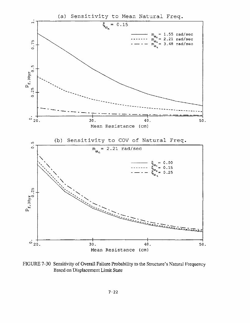
(a) Sensitivity to Mean Natural Freq.
s = 0.15ro"
a
m = 1.55 rad/secco"m = 2.21 rad/secCOil
m = 3.48 rad/secco~
------ ------- ------------
......
... ...............
............................
----~---------------
0 20 . 30. 40.
Mean Resistance (em)50.
(b) Sensitivity to COV of Natural Freq.Lf)-r- -.,
a m = 2.21 rad/secrot)
0.000.150.25
0 20 . 30. 40.
Mean Resistance (em)50.
FIGURE 7-30 Sensitivity of Overall Failure Probability to the Structure's Natural FrequencyBased on Displacement Limit State
7-22
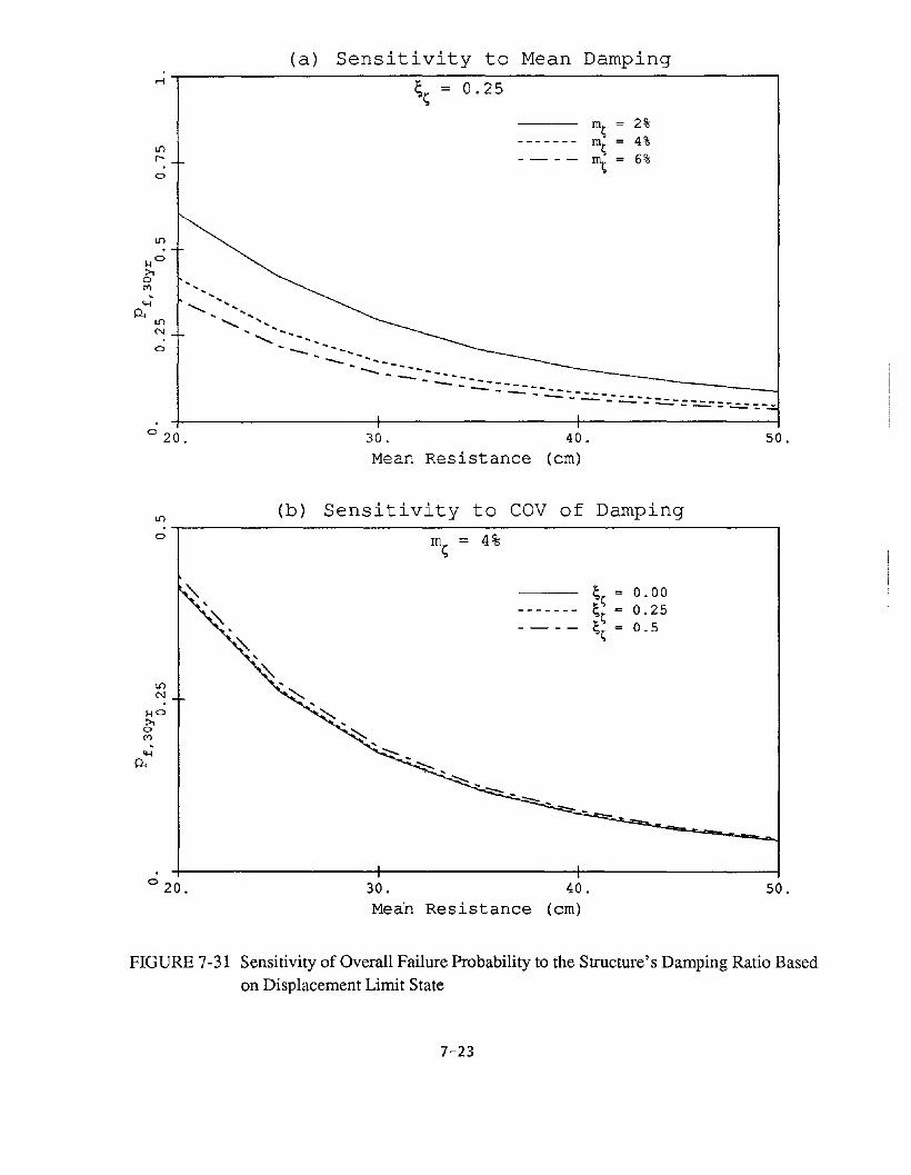
Lf)
r-
o
o
(a) Sensitivity to Mean Damping
~~ = 0.25
m = 2%~m = 4%~m = 6%~
""'""-- ........ ............ --::.- .... _---
.... -- .... :.:...-:~:-----....-.:.:,.-....-.:.:..."":""-=--=-:..=: =--=.= -=.- ....
° 20.
o
30. 40.
Mean Resistance (cm)
(b) Sensitivity to COV of Damping
m~ = 4%
50.
;\.. ~~ = 0.00
~------- ~~ = 0.25- - -- ~~ = 0.5
~ ,~
Lf)
~N
HO ~>t0C'1
....0..
~
:::00-::::-.
::::-- - ::.-- -
° 20. 30. 40.
Mean Resistance (cm)50.
FIGURE 7-31 Sensitivity of Overall Failure Probability to the Structure's Damping Ratio Basedon Displacement Limit State
7-23

(a) Sensitivity to Mean Natural Freq.
m = 1.55 rad/secco"m = 2.21 rad/secco"m = 3.48 rad/seccot\
'- -- -- ------ ---------------------
'-
--- --- --- ----
,
~ = 0.15(ill)
,\
\
\
\If)
r-
If)
<:)
<:)
If)
N
<:) 0.25 1.25 2.25
Mean Resistance (m/sec2)
3.25
(b) Sensitivity to COV of Natural Freq.rl.----------------------------------.
m = 2.21 rad/secCO/1
If)
r-<:)
<:)
<:) 0.25 1.25 2.25
Mean Resistance (m/sec2)
3.25
FIGURE 7-32 Sensitivity of Overall Failure Probability to the Structure's Natural Frequency
Based on Acceleration Limit State
7-24
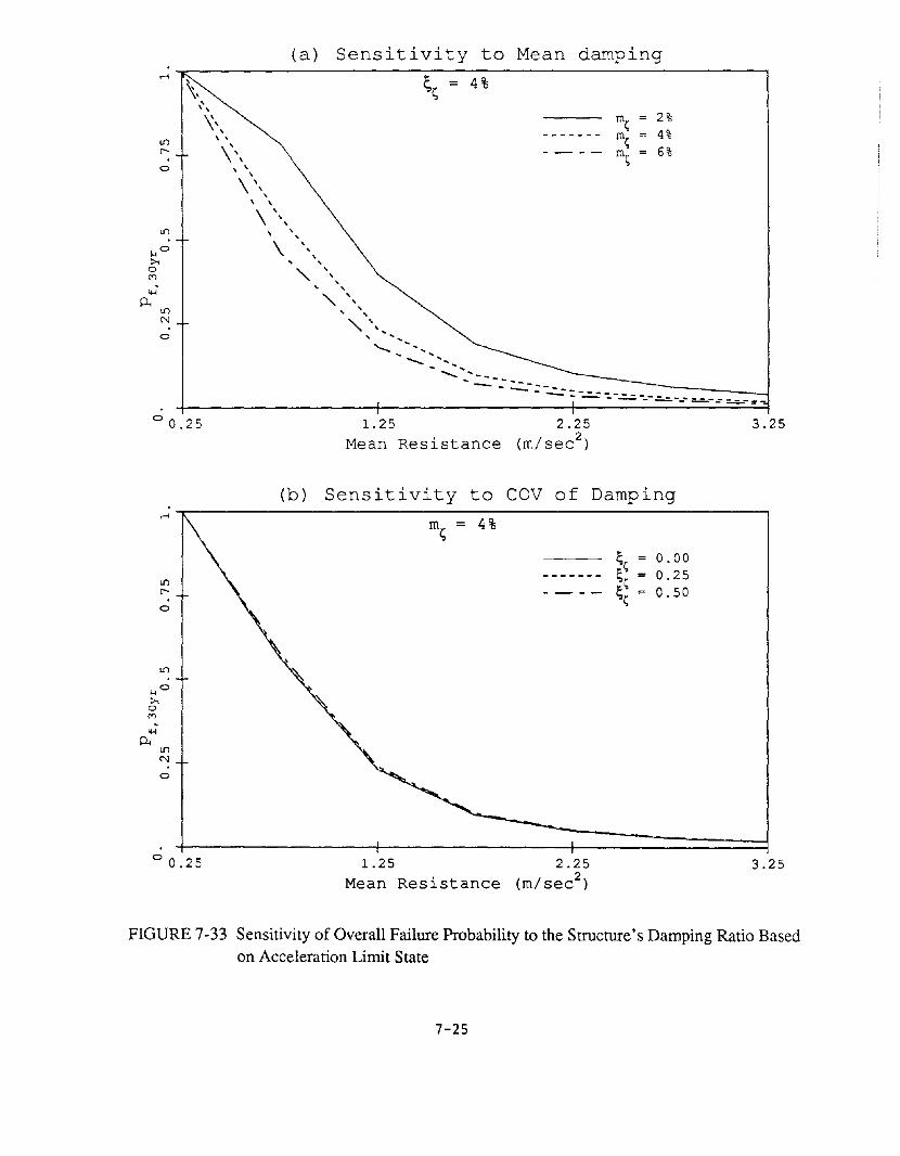
o
o
LJ)
N
o
(a) Sensitivity to Mean damping
~ := 4%~
m~ = 2%m = 4%
~m~ = 6%
1.25 2.25
Mean Resistance (m/sec2)
(b) Sensitivity to COV of Damping
m~ = 4%
0.000.250.50
3.25
1.25
Mean Resistance2.25
(m/ sec2)
3.25
FIGURE 7-33 Sensitivity of Overall Failure Probability to the Structure's Damping Ratio Basedon Acceleration Limit State
7-25


8. Conclusion
Based on two limit states, defined in terms of relative displacement and pseudo
acceleration at the deck level, and for several combinations of earthquake and sea-storm
loads, this report demonstrates the short-term and long-term multi-hazard risk analysis of
an offshore platform. It also determines the influence of ambient load on the earthquake
safety, and the effect of parameter uncertainty on failure probabilities in general. Based on
the cases studied, the following conclusions can be drawn:
1) The relative importance of loads largely depend on the limit state and the structure's
natural frequency. For a flexible offshore structure, we show that while in the case
of a displacement limit state the sea-storm load dominates, the same load is not
important in relation to an acceleration limit state. If a deflection limit state governs
the design, the margin of safety against earthquake load may be quite large.
2) The coincidental load due to the simultaneous occurrence of earthquake and sea-storm
does not influence the long-term risk of offshore structures perceptibly. However, if
the resistance level is very high, it could be of greater relative importance.
3) The ambient load increases the risk due to earthquake alone, especially at lower
resistance levels.
4) The failure probabilities are exceedingly sensitive to the mean and the variability
of a structure's natural frequency. Obtaining more and better information through
ambient vibration testing or other means is likely to be very beneficial, with respect
to safety and economy.
5) The statistical uncertainty of load and structural parameters affects failure proba
bilities in a complex manner. Depending on the load intensity, for instance, this
uncertainty may either increase or decrease the conditional fragility. However, it al
ways leads to an increase in the unconditional and overall failure probabilities. Also,
the effect is sensitive to the type of limit state; in the case study, it is found to be more
pronounced for the displacement limit state than for the acceleration limit state.
6) In related work in progress, we are extending the methodology to multi-degree models
of the structure and to limit states that are not of the first-passage type, notably,
8-1

fatigue failure and excessive inelastic deformation. Uncertainty in event duration
and the parameters of the long-term load occurrence distributions are also to be
incorporated in the model.
8-2
References
1) Benjamin, J.R., and Cornell, C.A., "Probability, Statistics, and Decision for Civil
Engineers," McGraw-Hill, New York.
2) Berge, B., and Penzien, J., "Three-dimensional stochastic response of offshore towers
to wave forces," Offshore Technology Conferences, Dallas, Texas, OTC 2050, 1974.
3) Bernreuter, D.L., Sary, J.B., Mensing, R.W., and Chung, D.H., "Seismic hazard
characterization of the Eastern United States: Methodology and interim results for
ten sites," Report for U.S. Nuclear Regulatory Commission, NUREG/CR-3756, April
1984.
4) Davenport, A.G., "Gust loading factors," Journal of the structural Division, ASCE,
June 1967.
5) Davenport, A.G., "Note on the random distribution of the largest value of a random
function with emphasis on gust loading," Proc. Inst. of Civil Engineers, London,
Vol. 28, 1964.
6) Kallberg, K., "Seismic risk in Southern California," M.l. T. Dept. of Civil Engineering
Research Report R69-31, June 1969.
7) Kanai, K., "An empirical formula for the spectrum of strong earthquake motion,"
Bull. Earthq. Res. Inst., U. of Tokyo, Vol. 39, 85-95, Tokyo.
8) Kryloff, N., and Bogoliaboff, N., "Introduction to nonlinear mechanics: Approximate
asymptotic methods," Princeton University Press, 11, 1943.
9) Malhotra, A., and Penzien, J., "Stochastic analysis of offshore structures," Earhquake
Eng. Res. Ctr. Report No. 69-6, U. of California, Berkeley, Calif. 1969.
10) Morison, J.R., Obrien, M.P., Johnson, J.W., and Schaaf, S.A., "The force exerted by
surface waves on piles," Amer. Inst. Min. Eng. Petrol Trans., TP 2846, Vol. 189,
pp. 149-154, 1950.
11) Pierson, W.J., and Moskowitz, Z., "A proposed spectral form for fully developed wind
seas based on the similarity theory of S.A. Kitaigorodskii," Journal of Geophysical
Research, Vol. 69, nr. 24, Dec. 1964.
9-1

12) Roberts, J.B., "First-passage probabilities for randomly excited systems: Diffusion
methods," Probabilistic Engineering Mechanics, Vol. 1, NO.2 1986.
13) Vanmarcke, E.H., "Spatial averaging of earthquake ground motion: the effect on
response spectra," Proceedings EPRI Workshop on Engineering Characterization of
Small-magnitude Earthquakes, 1987.
14) Vanmarcke, E.H., "On the distribution of the first-passage time for normal stationary
random process," Journal of Applied Mechanics, March 1975.
15) Wen, Y.K., "Methods for reliability of structures under multiple time varying loads,"
Journal of Nuclear Engineering and Design, Vol. 60, pp. 61-70 1980.
16) Wilson, J.F., "Dynamics of offshore structures," John Wiley & Sons, NewYork 1984.
9-2

NATIONAL CENTER FOR EARTHQUAKE ENGINEERING RESEARCHLIST OF PUBLISHED TECHNICAL REPORTS
The National Center for Earthquake Engineering Research (NCEER) publishes technical reports on a variety of subjects relatedto earthquake engineering written by authors funded through NCEER. These reports are available from both NCEER'sPublications Department and the National Technical Information Service (NTIS). Requests for reports should be directed to thePublications Department, National Center for Earthquake Engineering Research, State University of New York at Buffalo, RedJacket Quadrangle, Buffalo, New York 14261. Reports can also be requested through NTIS, 5285 Port Royal Road, Springfield,Virginia 22161. NTIS accession numbers are shown in parenthesis, if available.
NCEER-87-0001
NCEER-87-0002
NCEER-87-0003
NCEER-87-0004
NCEER-87-0005
NCEER-87-0006
NCEER-87-0007
NCEER-87-0008
NCEER-87-0009
NCEER-87-0010
NCEER-87-0011
NCEER-87-0012
NCEER-87-0013
NCEER-87-0014
NCEER-87-0015
NCEER-87-0016
NCEER-87-0017
"First-Year Program in Research, Education and Technology Transfer," 3/5/87, (PB88-134275/AS).
"Experimental Evaluation of Instantaneous Optimal Algorithms for Structural Control," by R.C. Lin,T.T. Soong and AM. Reinhorn, 4/20/87, (PB88-134341/AS).
"Experimentation Using the Earthquake Simulation Facilities at University at Buffalo," by A.M.Reinhorn and RL Ketter, to be published.
"The System Characteristics and Performance of a Shaking Table," by lS. Hwang, K.C. Chang andG.C. Lee, 6/1/87, (PB88-134259/AS).
"A Finite Element Formulation for Nonlinear Viscoplastic Material Using a Q Model," by O. Gyebi andG. Dasgupta, 11/2/87, (PB88-213764/AS).
"Symbolic Manipulation Program (SMP) - Algebraic Codes for Two and Three Dimensional FiniteElement Formulations," by X. Lee and G. Dasgupta, 11/9/87, (PB88-219522/AS).
"Instantaneous Optimal Control Laws for Tall Buildings Under Seismic Excitations," by J.N. Yang, A.Akbarpour and P. Ghaemmaghami, 6/10/87, (PB88-134333/AS).
"IDARC: Inelastic Damage Analysis of Reinforced Concrete-Frame Shear-Wall Structures," by Y.lPark, AM. Reinhorn and S.K. Kunnath, 7/20/87, (PB88-134325/AS).
"Liquefaction Potential for New York State: A Preliminary Report on Sites in Manhattan and Buffalo,"by M. Budhu, V. Vijayakumar, R.F. Giese and L. Baumgras, 8/31/87, (PB88-163704/AS).
"Vertical and Torsional Vibration of Foundations in Inhomogeneous Media," by A.S. Veletsos andKW. Dotson, 6/1/87, (PB88-134291/AS).
"Seismic Probabilistic Risk Assessment and Seismic Margins Studies for Nuclear Power Plants," byHoward H.M. Hwang, 6/15/87, (PB88-134267/AS).
"Parametric Studies of Frequency Response of Secondary Systems Under Ground-AccelerationExcitations," by Y. Yong and Y.K. Lin, 6/10/87, (PB88-134309/AS).
"Frequency Response of Secondary Systems Under Seismic Excitation," by I.A HoLung, J. Cai andY.K. Lin, 7/31/87, (PB88-134317/AS).
"Modelling Earthquake Ground Motions in Seismically Active Regions Using Parametric Time SeriesMethods," G.W. Ellis and AS. Cakmak, 8/25/87, (PB88-134283/AS).
"Detection and Assessment of Seismic Structural Damage," by E. DiPasquale and AS. Cakmak,8/25/87, (PB88-163712/AS).
"Pipeline Experiment at Parkfield, California," by l Isenberg and E. Richardson, 9/15/87,(PB88-163720/AS).
"Digital Simulation of Seismic Ground Motion," by M. Shinozuka, G. Dcodatis and T. Harada, 8/31/87,(PB88-155197/AS).
A-I

NCEER-87-0018
NCEER-87-0019
NCEER-87-0020
NCEER-87-0021
NCEER-87-0022
NCEER-87-0023
NCEER-87-0024
NCEER-87-0025
NCEER-87-0026
NCEER-87-0027
NCEER-87-0028
NCEER-88-0001
NCEER-88-0002
NCEER-88-0003
NCEER-88-0004
NCEER-88-0005
NCEER-88-0006
NCEER-88-0007
NCEER-88-0008
"Practical Considerations for Structural Control: System Uncertainty, System Time Delay and Truncation of Small Control Forces," I Yang and A Akbarpour, 8/10/87, (PB88-163738/AS).
"Modal Analysis of Nonclassically Damped Structural Systems Using Canonical Transformation," byJ.N. Yang, S. Sarkani and F.x. Long, 9/27/87, (PB88-187851/AS).
"A Nonstationary Solution in Random Vibration Theory," by IR. Red-Horse and P.D. Spanos, 11/3/87,(PB88-163746/AS).
"Horizontal Impedances for Radially Inhomogeneous Viscoelastic Soil Layers," by AS. Veletsos andKW. Dotson, 10/15/87, (PB88-150859/AS).
"Seismic Damage Assessment of Reinforced Concrete Members," by Y.S. Chung, C. Meyer and M.Shinozuka, 10/9/87, (PB88-150867/AS).
"Active Structural Control in Civil Engineering," by T.T. Soong, 11/11/87, (PB88-187778/AS).
"Vertical and Torsional Impedances for Radially Inhomogeneous Viscoelastic Soil Layers," by K.W.Dotson and A.S. Veletsos, 12/87, (PB88-187786/AS).
"Proceedings from the Symposium on Seismic Hazards, Ground Motions, Soil-Liquefaction andEngineering Practice in Eastern North America, October 20-22, 1987, edited by K.H. Jacob, 12/87,(PB88-188115/AS).
"Report on the Whittier-Narrows, California, Earthquake of October 1, 1987," by I Pantelic and AReinhorn, 11/87, (PB88-187752/AS).
"Design of a Modular Program for Transient Nonlinear Analysis of Large 3-D Building Structures," byS. Srivastav and IF. Abel, 12/30/87, (PB88-l87950/AS).
"Second-Year Program in Research, Education and Technology Transfer," 3/8/88, (PB88-219480/AS).
"Workshop on Seismic Computer Analysis and Design of Buildings With Interactive Graphics," by J.F.Abel and C.H. Conley, 1/18/88, (PB88-187760/AS).
"Optimal Control of Nonlinear Flexible Structures," IN. Yang, FX. Long and D. Wong, 1/22/88,(PB88-213772/AS).
"Substructuring Techniques in the Time Domain for Primary-Secondary Structural Systems," by G. D.Manolis and G. Juhn, 2/10/88, (PB88-213780/AS).
"Iterative Seismic Analysis of Primary-Secondary Systems," by A Singhal, L.D. Lutes and P. Spanos,2/23/88, (PB88-213798/AS).
"Stochastic Finite Element Expansion for Random Media," P. D. Spanos and R. Ghanem, 3/14/88,(PB88-213806/AS).
"Combining Structural Optimization and Structural Control," F. Y. Cheng and C. P. Pantelides, 1/10/88,(PB88-213814/AS).
"Seismic Performance Assessment of Code-Designed Structures," H.H-M. Hwang, J-W. Jaw and H-J.Shau, 3/20/88, (PB88-219423/AS).
"Reliability Analysis of Code-Designed Structures Under Natural Hazards," H.H-M. Hwang, H. Ushibaand M. Shinozuka, 2/29/88.
A-2

NCEER-88-0009
NCEER-88-0010
NCEER-88-0011
NCEER-88-0012
NCEER-88-0013
NCEER-88-0014
NCEER-88-0015
NCEER-88-0016
NCEER-88-0017
NCEER-88-0018
NCEER-88-0019
NCEER-88-0020
NCEER-88-0021
NCEER-88-0022
NCEER-88-0023
"Seismic Fragility Analysis of Shear Wall Structures," J-W Jaw and H.H-M. Hwang, 4/30/88.
"Base Isolation of a Multi-Story Building Under a Harmonic Ground Motion - A Comparison ofPerformances of Various Systems," F-G Fan, G. Ahmadi and I.G. Tadjbakhsh, 5/18/88.
"Seismic Floor Response Spectra for a Combined System by Green's Functions," F.M. Lavelle, L.A.Bergman and P.D. Spanos, 5/1/88.
"A New Solution Technique for Randomly Excited Hysteretic Structures," G.Q. Cai and Y.K. Lin,5/16/88.
"A Study of Radiation Damping and Soil-Structure Interaction Effects in the Centrifuge," K. Weissman,supervised by lH. Prevost, 5/24/88.
"Parameter Identification and Implementation of a Kinematic Plasticity Model for Frictional Soils," J.H.Prevost and D.V. Griffiths, to be published.
"Two- and Three-Dimensional Dynamic Finite Element Analyses of the Long Valley Dam," D.V.Griffiths and lH. Prevost, 6/17/88.
"Damage Assessment of Reinforced Concrete Structures in Eastern United States," A.M. Reinhorn, M.lSeidel, S.K. Kunnath and Y.l Park, 6/15/88.
"Dynamic Compliance of Vertically Loaded Strip Foundations in Multilayered Viscoelastic Soils," S.Ahmad and A.S.M. Israil, 6/17/88.
"An Experimental Study of Seismic Structural Response With Added Viscoelastic Dampers," R.C. Lin,Z. Liang, T.T. Soong and R.H. Zhang, 6/30/88.
"Experimental Investigation of Primary - Secondary System Interaction," G.D. Manolis, G. Juhn andA.M. Reinhorn, 5/27/88.
"A Response Spectrum Approach For Analysis of NoncJassically Damped Structures," J.N. Yang, S.Sarkani and F,X, Long, 4/22/88.
"Seismic Interaction of Structures and Soils: Stochastic Approach," A.S. Veletsos and A.M. Prasad,7/21/88.
"Identification of the Serviceability Limit State and Detection of Seismic Structural Damage," E.DiPasquale and A.S. Cakmak, 6/15/88.
"Multi-Hazard Risk Analysis: Case of a Simple Offshore Structure," B.K. Bhartia and E.H. Vanmarcke,7/21/88.
A-3