multi-core symbolic bisimulation minimisation · int j softw tools technol transfer (2018)...

Int J Softw Tools Technol Transfer (2018) 20:157–177https://doi.org/10.1007/s10009-017-0468-z

TACAS 2016

Multi-core symbolic bisimulation minimisation

Tom van Dijk1 · Jaco van de Pol2

Published online: 2 August 2017© The Author(s) 2017. This article is an open access publication

Abstract We introduce parallel symbolic algorithms forbisimulationminimisation, to combat the combinatorial statespace explosion along three different paths. Bisimulationminimisation reduces a transition system to the small-est system with equivalent behaviour. We consider strongand branching bisimilarity for interactive Markov chains,which combine labelled transition systems and continuous-time Markov chains. Large state spaces can be representedconcisely by symbolic techniques, based on binary deci-sion diagrams. We present specialised BDD operations tocompute the maximal bisimulation using signature-basedpartition refinement. We also study the symbolic representa-tion of the quotient system and suggest an encoding basedon representative states, rather than block numbers. Ourimplementation extends the parallel, shared memory, BDDlibrary Sylvan, to obtain a significant speedup on multi-coremachines. We propose the usage of partial signatures andof disjunctively partitioned transition relations, to increasethe parallelisation opportunities. Also our new parallel datastructure for block assignments increases scalability.We pro-vide SigrefMC, a versatile tool that can be customised forbisimulation minimisation in various contexts. In particu-lar, it supports models generated by the high-performance

Work funded by the NWO Grant 612.001.101 (MaDriD) and by FWF,NFN Grant S11408-N23 (RiSE).

B Tom van [email protected]

Jaco van de [email protected]

1 Institute for Formal Methods and Verification, JohannesKepler University, Linz, Austria

2 Formal Methods and Tools, University of Twente, Enschede,The Netherlands

model checker LTSmin, providing access to specifications inmultiple formalisms, including process algebra. The exten-sive experimental evaluation is based on various benchmarksfrom the literature. We demonstrate a speedup up to 95× forcomputing the maximal bisimulation on one processor. Inaddition, we find parallel speedups on a 48-core machine ofanother 17× for partition refinement and 24× for quotientcomputation. Our new encoding of the reduced state spaceleads to smaller BDD representations, with up to a 5162-foldreduction.

Keywords Bisimulation minimisation · Interactive Markovchains · Binary decision diagrams · Parallel algorithms

1 Introduction

One of the main challenges for model checking is that thespace and time requirements of model checking algorithmsincrease exponentially in the size of the models. This papercombines state space reduction, symbolic representation, andparallel computation, to alleviate the state space explosion.

As input models, we consider interactive Markov chains(IMC). These provide a compositional framework to studyfunctionality, performance, and dependability of reactivesystems. IMCs inherit non-deterministic choice and commu-nication from labelled transition systems, and probabilistictimed (Markovian) transitions from continuous-timeMarkovchains.

A state space reduction computes the smallest “equiva-lent”model.Weconsider strongbisimilarity,whichpreservesall behaviour, and branching bisimilarity, which abstractsfrom internal behaviour (represented by τ -steps) and onlypreserves the observable behaviour. Note that branchingbisimulation preserves the branching structure of an LTS,

123

http://crossmark.crossref.org/dialog/?doi=10.1007/s10009-017-0468-z&domain=pdf

158 T. van Dijk, J. van de Pol

thus preserving all properties expressible in CTL*-X [14].These notions correspond to strong and branching lumpingfor IMCs.

The reduced state space consists of (representatives of) theequivalence classes in the largest bisimulation, which is typ-ically computed using partition refinement. Starting with theinitial partition, in which all states are equivalent, the currentpartition is refined until the states in any equivalence classcan no longer be distinguished. Blom et al. [5] introduceda signature-based method, which defines the equivalenceclasses according to the characterising signature of a state.

Another important technique to handle large state spacesis symbolic representation. Sets of states are representedby characteristic functions, which are efficiently stored inbinary decision diagrams (BDDs). In the literature, symbolicmethods have been applied to bisimulation minimisation inseveral ways. Bouali and De Simone [8] refine the equiv-alence relation R ⊆ S × S, by iteratively removing all“bad” pairs from R, i.e., pairs of states that are no longerequivalent. For strong bisimulation,Mumme andCiardo [32]apply saturation-based methods to compute R. Wimmeret al. [40,41] use signatures to refine the partition, repre-sented by the assignment to equivalence classes P : S → C .Symbolic bisimulation based on signatures has also beenapplied to Markov chains by Derisavi [16] and Wimmer etal. [38,39].

The symbolic representation of the reduced state spacetends to be much larger than the original model. One particu-lar application of symbolic bisimulation minimisation is as abridge between symbolical models and explicit-state analy-sis algorithms. Symbolical models can have very large statespaces that are efficiently encoded using BDDs. The min-imised model has often a sufficiently small number of states,so it can be further analysed efficiently using explicit-statealgorithms.

Symbolic techniques mainly reduce the memory require-ments of model checking. To speed up the computation,developing scalable parallel algorithms is the way forward,since it takes advantage of multi-core computer systems.In [17,18,20], we implemented the multi-core BDD pack-age Sylvan, providing parallel BDD operations to symbolicmodel checking.

Parallelisation had been applied to explicit-state bisimu-lation minimisation before. Blom et al. [4,5] introduced dis-tributed signature-based bisimulation reduction. Also, [29]proposed a concurrent algorithm for bisimulation minimisa-tion which combines signatures with the approach by Paigeand Tarjan [33]. Recently,Wijs [37] implemented highly par-allel strong and branching bisimilarity checking onGPGPUs.As far as we are aware, no earlier work combines symbolicbisimulation minimisation and parallelism. This paper is anextended version of [21]. There, we demonstrated that spe-cialised BDD operations for signature refinement provide a

major speedup of the sequential algorithm, and scale acrossmultiple processors.

We extend [21] by four new results. First, we investigatehow to compute the reduced state space, i.e., the quotient ofthe original system with respect to the maximal bisimulationobtained by signature refinement. Traditionally, the quotientis computed by a sequence of standard BDD operations.Similar to computing the partition, we find that quotient com-putation benefits from specialised BDD operations. Second,we study the representation of the quotient. Traditionally,its states are encoded by using the assigned block numberas state identifier. We improve the encoding by choosingone representative state from each block. This considerablyreduces the size of the resulting BDD representation. Third,we refine our algorithm. Instead of using a monolithic tran-sition relation, we now support a disjunctive partitioningof the transition relation. This appears to be more efficientthan a monolithic transition relation and provides furtherparallelisation opportunities when computing the maximalbisimulation. Finally, we link the tool SigrefMC presentedin [21] to LTSmin, by supporting the partitioned transitionsystems generated by the symbolic backend of the LTSmintoolset [6,28,31]. Since LTSmin supports various input lan-guages, including the specification language mCRL2 [13]for process algebra, this allows us to carry out a considerablylarger set of experiments, generated from various specifica-tion languages.

Outline This paper presents the following contributions.We recapitulate the notion of partition refinementwith partialsignatures in Sect. 3. Section 4 discusses how we extendedSylvan to parallelise signature-based partition refinement. Inparticular, we develop three specialised BDD algorithms: therefine algorithm refines a partition according to a signa-ture, but maximally reuses the block number assignment ofthe previous partition (Sect. 4.3). This algorithm improvesthe operation cache usage for the computation of the signa-tures of stable blocks and enables partition refinement withpartial signatures. The inert algorithm removes all transi-tions that are not inert (Sect. 4.4). This algorithm avoids anexpensive intermediate result reported in the literature [41].We discuss the new quotient computation in Sect. 5. Spe-cialised BDD algorithms significantly speed up the quotientcomputation for the interactive transition relation (Sect. 5.1)and for theMarkovian transition relation (Sect. 5.2). The newencoding of the quotient space is explained in Sect. 5.3. Sec-tion 6 presents the implementation of these algorithms as aversatile tool that can be customised for bisimulation min-imisation in various contexts, including support for transitionsystems generated by the model checking toolset LTSmin(Sect. 6.1). Section 7 discusses experimental data based onbenchmarks from the literature. For partition refinement, wedemonstrate a speedup of up to 95× sequentially. In addition,

123

Multi-core symbolic bisimulation minimisation 159

we find parallel speedups of up to 17× due to parallelisationwith 48 cores. For quotient computation, we find a speedupof 2–10× by using specialised operations, and we find sig-nificantly smaller BDDs (up to 5162× smaller) when usinga representative state rather than the block number to encodethe new transition system.

2 Preliminaries

We recall the basic definitions of partitions, of labelledtransition systems, of continuous-time Markov chains, ofinteractive Markov chains, and of various bisimulations asin [5,26,40–42].

2.1 Partitions

Definition 1 Given a set S, a partition π of S is a subsetπ ⊆ 2S such that

⋃

C∈π

C = S and ∀C,C ′ ∈ π : (C = C ′ ∨ C ∩ C ′ = ∅)

.

The elements ofπ are called equivalence classes or blocks.If π ′ and π are two partitions, then π ′ is a refinement of π ,written π ′ π , if each block of π ′ is contained in a block ofπ . Each equivalence relation ≡ is associated with a partitionπ = S/≡. In this paper, we use π and ≡ interchangeably.

2.2 Transition systems

Definition 2 A labelled transition system (LTS) is a tuple(S,Act, T ), consisting of a set of states S, a set of labelsAct, which may contain the non-observable action τ , andtransitions T ⊆ S × Act × S.

We write sa→ t for (s, a, t) ∈ T and s

τ� when s has

no outgoing τ -transitions. We usea∗→ to denote the transitive

reflexive closure ofa→. Given an equivalence relation ≡,

we writea→≡ for

a→∩≡, i.e., transitions between equivalentstates, called inert transitions. We use

a∗→≡ for the transitivereflexive closure of

a→≡ .

Definition 3 A continuous-time Markov chain (CTMC) is atuple (S,R), consisting of a set of states S and Markoviantransitions R : S → S → R≥0.

We write sλ⇒ t for R(s)(t) = λ. The interpretation of

sλ⇒ t is that the CTMC can switch from s to t within d time

units with probability 1−e−λ·d . For a state s, we denote withR(s)(C) = ∑

s′∈C R(s)(s′) the cumulative rate to reach a setof states C ⊆ S from state s in one transition.

Definition 4 An interactive Markov chain (IMC) is a tuple(S,Act, T,R), consisting of a set of states S, a set of labelsAct that may contain the non-observable action τ , transitionsT ⊆ S ×Act× S, and Markovian transitions R : S → S →R≥0.

An IMC basically combines the features of an LTS and aCTMC [25,26]. One feature of IMCs is themaximal progressassumption. Internal interactive transitions, i.e., τ -transitions,can be assumed to take place immediately, while the prob-ability that a Markovian transition executes immediately iszero. Therefore, we may remove all Markovian transitionsfrom states that have outgoing τ -transitions: s

τ→ impliesR(s)(S) = 0. We call IMCs to which this operation has beenapplied maximal-progress-cut (mp-cut) IMCs. In the rest ofthis paper, we implicitly assume that IMCs are mp-cut.

2.3 Bisimulation

We recall strong and branching bisimulation. All discussedbisimulations are equivalence relations on the states of a tran-sition system. Two states are bisimilar if and only if there is abisimulation that relates them. So the maximal bisimulationrelates two states if and only if they are bisimilar. For LTSs,we define strong and branching bisimulation as follows [41]:

Definition 5 A strong bisimulation on an LTS is an equiva-lence relation ≡S such that for all states s, t, s′ with s ≡S tand s

a→ s′, there is a state t ′ with t a→ t ′ and s′ ≡S t ′.

Definition 6 A branching bisimulation on an LTS is anequivalence relation ≡B such that for all states s, t, s′ withs ≡B t and s

a→ s′, either

– a = τ and s′ ≡B t , or– there are states t ′, t ′′ with t

τ∗→ t ′ a→ t ′′ and t ≡B t ′ ands′ ≡B t ′′.

For CTMCs, we define strong bisimulation as follows [16,38]:

Definition 7 A strong bisimulation on a CTMC is an equiv-alence relation ≡S such that for all (s, t) ∈ ≡S and for allclasses C ∈ S/≡S , R(s)(C) = R(t)(C).

For mp-cut IMCs, we define strong and branching bisim-ulation as follows [26,42]:

Definition 8 A strong bisimulation on an mp-cut IMC is anequivalence relation ≡S such that for all (s, t) ∈ ≡S and forall classes C ∈ S/≡S ,

– sa→ s′ for some s′ ∈ C implies t

a→ t ′ for some t ′ ∈ C– R(s)(C) = R(t)(C)

123


Definition 9 A branching bisimulation on an mp-cut IMC isan equivalence relation ≡B such that for all (s, t) ∈ ≡B andfor all classes C ∈ S/≡B ,

– sa→ s′ for some s′ ∈ C implies

• a = τ and (s, s′) ∈≡B , or• there are states t ′, t ′′ ∈ S with t

τ∗→ t ′ a→ t ′′ and(t, t ′) ∈≡B and t ′′ ∈ C .

– R(s)(C) > 0 implies

• R(s)(C) = R(t ′)(C) for some t ′ ∈ S such that tτ∗→

t ′ τ� and (t, t ′) ∈≡B .

– sτ� implies t

τ∗→ t ′ τ� for some t ′

As we compare our work to [41,42], we considerdivergence-sensitive branchingbisimulation for IMCs,whichdistinguishes deadlock states (without successors) fromstates that only have self-looping transitions.

3 Signature-based bisimulation minimisation

Blom and Orzan [5] introduced a signature-based approachto compute the maximal bisimulation of an LTS, which wasfurther developed into a symbolic method by Wimmer etal. [41]. Each state is characterised by a signature, whichis the same for all equivalent states in a bisimulation. Thesesignatures are used to refine a partition of the state space untila fixed point is reached, which is the maximal bisimulation.

In the literature, multiple signatures are sometimes usedthat together fully characterise states, for example based onthe state labels, based on the rates of continuous-time tran-sitions, and based on the enabled interactive transitions. Weconsider these multiple signatures as elements of a singlesignature that fully characterises each state.

Definition 10 A signature σ(π)(s) is a tuple of functionsfi (π)(s), that together characterise each state s with respectto a partition π . Two signatures σ(π)(s) and σ(π)(t) areequivalent, if and only if for all fi , fi (π)(s) = fi (π)(t).

The signatures of the five bisimulations from Sect. 2.3are known from the literature. First, we define for all actionsa ∈ Act and equivalence classes C ∈ π :

– T(π)(s) = {(a,C) | ∃s′ ∈ C : s a→ s′}– B(π)(s) = {(a,C) | ∃s′ ∈ C : s τ∗→

π

a→ s′ ∧ ¬(a =τ ∧ s ∈ C)}

– Rs(π)(s) = C �→ R(s)(C)

– Rb(π)(s) = C �→ max({R(s′)(C) | ∃s′ : s τ∗→πs′ τ

�})

The five bisimulations are associated with the following sig-natures:

Strong bisimulation for LTS (T) [41]Branching bisimulation for LTS (B) [41]Strong bisimulation for CTMC (Rs) [38]Strong bisimulation for IMC (T,Rs) [42]Branching bisimulation for IMC (B,Rb, s

τ∗→ τ�) [42]

FunctionsT andB assign to each state s all pairs of actionsa and equivalence classes C ∈ π , such that state s can reachC by an action a either directly (T) or via any number of inertτ -steps (B). Furthermore, inert τ -steps are removed from B.Rs equalsR but with the domain restricted to the equivalenceclasses C ∈ π and represents the cumulative rate with whicheach state s can go to states inC .Rb equalsRs for states s

τ�

and takes the highest “reachable rate” for states with inert τ -transitions. In branching bisimulation for mp-cut IMCs, the“highest reachable rate” is by definition the rate that all statess

τ� inC have. The element s

τ∗→ τ� distinguishes time conver-

gent states from time divergent states [42] and is independentof the partition.

For the bisimulations of Definitions 5–9, we state:

Lemma 1 A partition π is a bisimulation, iff for all s and tthat are equivalent in π , σ(π)(s) = σ(π)(t).

For the above definitions, it is fairly straightforward toprove that they are equivalent to the classical definitionsof bisimulation. See [5,41] for the bisimulations on LTSsand [42] for the bisimulations on IMCs.

3.1 Signature-based partition refinement

As discussed above, signatures can consist of multiple ele-ments. We first define partition refinement using the fullsignature. We then define partition refinement with partialsignatures, i.e., using the elements of the signature, and dis-cuss advantages of this approach.

Definition 11 (Partition refinement with full signatures)

sigref(π, σ ) := {{t ∈ S | σ(π)(s) = σ(π)(t)} | s ∈ S}

For a given signature σ , we define the series of partitionrefinements:

π0 := {S}πn+1 := sigref(πn, σ )

The algorithm iteratively refines the initial coarsest parti-tion {S} according to the signatures of the states, until somefixed point πn+1 = πn is obtained. For monotone signatures(defined below), this fixed point is the maximal bisimulation.

123


Definition 12 A signature is monotone if for all π, π ′ withπ π ′, σ(π)(s) = σ(π)(t) implies σ(π ′)(s) = σ(π ′)(t).

For all monotone signatures, the sigref operator is mono-tone: π π ′ implies sigref(π, σ ) sigref(π ′, σ ). Hence,following Kleene’s fixed point theorem, the procedure abovereaches the greatest fixed point.

In Definition 11, the full signature is computed in everyiteration. We propose to apply partition refinement usingparts of the signature. By definition, σ(π)(s) = σ(π)(t)if and only if for all parts fi (π)(s) = fi (π)(t).

Definition 13 (Partition refinement with partial signatures)

sigref(π, fi ) := {{t ∈ S | fi (π)(s) = fi (π)(t)∧s ≡π t} | s ∈ S}

π0 := {S}πn+1 := sigref(πn, fi ) (select fi ∈ σ)

We always select some fi that refines the partition π . Afixed point is reached only when no fi refines the partitionfurther: ∀ fi ∈ σ : sigref(πn, fi ) = πn . The extra clauses ≡π t ensures that every application of sigref refines thepartition.

Theorem 1 If all parts fi are monotone, Definition 13 yieldsthe greatest fixed point.

Proof The procedure terminates since the chain is decreasing(πn+1 πn), due to the added clause s ≡π t . We reachsome fixed point πn , since sigref(πn, σ ) = πn is impliedby ∀ fi ∈ σ : sigref(πn, fi ) = πn . Finally, to prove thatwe get the greatest fixed point, assume there exists anotherfixed point ξ = sigref(ξ, σ ). Then, also ξ = sigref(ξ, fi )for all i . We prove that ξ πn by induction on n. Initially,ξ S = π0. Assume ξ πn , then for the selected i , ξ =sigref(ξ, fi ) sigref(πn, fi ) = πn+1, using monotonicityof fi .

There are several advantages to this approach due to itsflexibility. First, for any fi that is independent of the par-tition, we need to refine with respect to that fi only once.Furthermore, refinements can be applied according to differ-ent strategies. For instance, for the strong bisimulation of anmp-cut IMC, one could refine w.r.t. T until there is no morerefinement, then w.r.t. Rs until there is no more refinement,then repeat until neitherT norRs refines the partition. Finally,computing the full signature is the most memory-intensiveoperation in symbolic signature-based partition refinement.If the partial signatures are smaller than the full signature,then larger models can be minimised.

4 Symbolic signature refinement

This section describes the parallel decision diagram librarySylvan, followed by the (MT)BDDs and (MT)BDD oper-ations required for signature-based partition refinement.We describe how we encode partitions and signatures forsignature-based partition refinement. We present a new par-allelisedrefine function thatmaximally reuses block num-bers from the old partition. Finally, we present a new BDDalgorithm that computes inert transitions, i.e., restricts a tran-sition relation such that states s and s′ are in the same block.

4.1 Decision diagram algorithms in Sylvan

In symbolic model checking [11], sets of states and transi-tions are represented by their characteristic function, ratherthan stored individually. With states described by N Booleanvariables, a set S ⊆ B

N can be represented by its character-istic function f : B

N → B, where S = {s | f (s)}. Binarydecision diagrams (BDDs) are a concise and canonical rep-resentation of Boolean functions [10].

An (ordered) BDD is a directed acyclic graph with leaves0 and 1. Each internal node has a variable label xi and twooutgoing edges labelled 0 and 1. Variables are encounteredalong each path according to a fixed variable ordering. Dupli-cate nodes and nodes with two identical outgoing edges areforbidden. It is well known that for a fixed variable ordering,every Boolean function is represented by a unique BDD.

In addition to BDDs with leaves 0 and 1, multi-terminalbinary decision diagrams have been proposed [2,12] withleaves other than 0 and 1, representing functions from theBoolean space B

N onto any set. For example, MTBDDscan have leaves representing integers (encoding B

N → N),floating-point numbers (encoding B

N → R), and rationalnumbers (encoding B

N → Q). Partial functions are sup-ported using a leaf ⊥.

Sylvan [17,18,20] implements parallelised operations ondecision diagrams using parallel data structures and work-stealing.Work-stealing [7,19] is a load balancing method fortask-based parallelism. Recursive operations, such as mostBDD operations, implicitly form a tree of tasks. Independentsubtasks are stored in queues and idle processors steal tasksfrom the queues of busy processors.

See Algorithm 1 for a generic example of a BDD opera-tion. This algorithm takes two inputs, the BDDs x and y, towhich a binary operationF is applied.Most decision diagramoperations first check if the operation can be applied immedi-ately to x and y (line 2). This is typically the case when x andy are leaves. Often there are also other trivial cases that canbe checked first. We then consult the operation cache (line 4)to see if this (sub)operation has been computed earlier. Theoperation cache is required to reduce the time complexity ofBDD operations from exponential to polynomial in the size

123


1 def apply(x , y, F):2 if x and y are leaves or trivial : return F(x, y)3 Normalise/simplify parameters4 if result ← cache[(x, y,F)] : return result5 v = topVar(x ,y)6 do in parallel:7 low ← apply(xv=0, yv=0, F)8 high ← apply(xv=1, yv=1, F)9 result ← lookupBDDnode(v, low, high)

10 cache[(x, y,F)] ← result11 return result

Algorithm 1 Example of a parallelised BDD algorithm: apply a binaryoperator F to BDDs x and y.

of the BDDs. Sylvan uses a single shared unique table forall BDD nodes and a single shared operation cache for alloperations.

Often, the parameters of an operation can be normalised insomeways to increase the cache efficiency. For example,a∧band b∧ a are the same operation. In that case, normalisationrules can rewrite the parameters to some standard form inorder to increase cache utilisation, at line 3. A well-knownexample is the if-then-else algorithm, which rewrites usingrewrite rules called “standard triples” as described in [9].

If x and y are not leaves and the operation is not trivialor in the cache, we use topVar (line 5) to determine thefirst variable of the root nodes of x and y. If x and y have adifferent variable in their root node, topVar returns the firstone in the variable ordering. We then compute the recursiveapplication of F to the cofactors of x and y with respect tovariable v at lines 7–8. We write xv=i to denote the cofactorof x where variable v takes value i . Since x and y are orderedaccording to the same fixed variable ordering, we can easilyobtain xv=i . If the root node of x is on the variable v, thenxv=i is obtained by following the low (i = 0) or high (i = 1)edge of x . Otherwise, xv=i equals x . After computing thesuboperations, we compute the result by either reusing anexisting or creating a new BDD node (line 9).

Operations on decision diagrams are typically recursivelydefined on the structure of the inputs. To parallelise the oper-ation in Algorithm 1, the two independent suboperations atlines 7–8 are executed in parallel using work-stealing. Toobtain high performance in a multi-core environment, thedata structures for the BDD node table and the operationcache must be highly scalable. Sylvan implements severalnon-blocking data structures to enable good speedups [17,20].

To compute symbolic signature-based partition refine-ment, several basic operationsmust be supported by theBDDpackage (see also [41]). Sylvan implements basic operationssuch as ∧ and if-then-else, and existential quantifi-cation ∃. Negation ¬ is performed in constant time usingcomplement edges. To compute relational products of tran-sition systems, there are operations relnext (to compute

successors) and relprev (to compute predecessors and toconcatenate relations), which combine the relational productwith variable renaming. Similar operations are also imple-mented for MTBDDs. Sylvan is designed to support customBDD algorithms. We present several new algorithms below.

4.2 Encoding of signature refinement

We implement symbolic signature refinement similar to [41].However, we do not refine the partition with respect to asingle block, but with respect to all blocks simultaneously.We use a binary encoding with variables s for the currentstate, s′ for the next state, a for the action labels, and b forthe blocks. We order BDD variables a and b after s and s′,since this is required to efficiently replace signatures (on aand b) by new block numbers b (see below). Variables s ands′ are interleaved, which is a common heuristic for transitionsystems.

In [21], we ordered a before b. However, we expect that ingeneral ordering b before a is better for the following reason.If we have a before b, then when computing the signaturesand the quotient (Sect. 5), it is guaranteed that all BDD nodeson a variables have to be recreated, whereas they may bereused if a variables are last in the ordering.

To perform symbolic bisimulation, we represent a numberof sets by their characteristic functions. See also Fig. 1.

– A set of states is represented by a BDD S(s);– Transitions are represented by a BDD T (s, s′, a);– Markovian transitions are represented by an MTBDDR(s, s′),with leaves containing rational numbers (Q) thatrepresent the transition rates;

– SignaturesT andB are represented by aBDDσT (s, b, a);– Signatures Rs and Rb are represented by an MTBDD

σR(s, b), with leaves containing rational numbers (Q)that represent the rates in the signature.

We represent Markovian transitions using rational num-bers, since they offer better precision than floating-pointnumbers. The manipulation of floating-point numbers typi-cally introduces tiny rounding errors, resulting in differentresults of similar computations. This significantly affectsbisimulation reduction, often resulting in finer partitions thanthe maximal bisimulation [38], which is unacceptable.

In the literature, three methods have been proposed torepresent the partition π .

1. As an equivalence relation, using a BDD E(s, s′) = 1 iffs ≡π s′ [8,32].

2. As a partition, by assigning each block a unique number,encoded with variables b, using a BDD P(s, b) = 1 iffs ∈ Cb [16,41,42].

123


s, s

a

T (s, s , a)

s

b

a

σT (s, b, a)

s

b

σR(s, b)

s

b

P(s , b)

Fig. 1 Schematic overview of the BDDs in signature refinement

3. Using k = � log2 n� BDDs P0, . . . ,Pk−1 such thatPi (s) = 1 iff s ∈ Cb and the ith bit of b is 1. Thisrequires significant time to restore blocks for the refine-ment procedure, but can require less memory [15].

We choose to use method 2, since in practice the BDD ofP(s, b) is smaller than the BDD of E(s, s′). Using P(s, b)also has the advantage of straightforward signature compu-tation. The logarithmic representation is incompatible withour approach, sincewe refine all blocks simultaneously.Theirapproach involves restoring individual blocks to the P(s, b)representation, performing a refinement step, and compact-ing the result to the logarithmic representation. Restoring allblocks simply computes the full P(s, b).

In the implementation of signature refinement, we actu-ally encode P using s′ variables instead of s variables, i.e.,encoding from target states to block numbers. This is advan-tageous for signature computation, as the signatures σT andσR can then be computed as follows:

– σT (s, b, a) := ∃s′ : T (s, s′, a) ∧ P(s′, b)– σR(s, b) := ∃sum s′ : R(s, s′) ∧ P(s′, b)

4.3 The refine algorithm

We present a new BDD algorithm to refine partitions accord-ing to a signature, which maximally preserves previouslyassigned block numbers.

Partition refinement consists of two steps: computing thesignatures and computing the next partition. Given the sig-natures σT and/or σR for the current partition π , the newpartition can be computed as follows.

Since the chosen variable ordering has variables s, s′before a, b, each path in σ ends in a (MT)BDD represent-ing the signature for the states encoded by that path. For σT ,every path that assigns values to s ends in a BDD on a, b. For

1 def refine(σ , P):2 if result ← cache[(σ,P, iter)] : return result3 v = topVar(σ , P) # interpret s′ in P as s4 if v equals si for some i :

# match state in σ and P5 do in parallel:6 low ← refine(σsi=0, Ps′i=0)

7 high ← refine(σsi=1, Ps′i=1)

8 result ← lookupBDDnode(s′i , low, high)

9 else:# σ now encodes the state signature# P now encodes the previous block

10 B ← decodeBlock(P)

# try to claim block B if still free11 if blocks[B].sig = ⊥ :12 cas(blocks[B].sig,⊥, σ )

13 if blocks[B].sig = σ :14 result ← P15 else:16 B ← search_or_insert(σ, B)

17 result ← encodeBlock(B)18 cache[(σ,P, iter)] ← result19 return result

Algorithm 2 refine, the (MT)BDD operation that assigns blocknumbers to signatures, given a signature σ and the previouspartition P .

σR , every path that assigns values to s ends in a MTBDD onb with rational leaves.

Wimmer et al. [41] present a BDD operation refinethat “replaces” these sub-(MT)BDDs by the BDD represent-ing a unique block number for each distinct signature. Theresult is the BDD of the next partition. They use a globalcounter and a hash table to associate each signature with aunique block number. This algorithm has the disadvantagethat block number assignments are unstable. There is no guar-antee that a stable block has the same block number in thenext iteration. This has implications for the computation ofthe new signatures. When the block number of a stable blockchanges, cached results of signature computation in earlieriterations cannot be reused.

123


We modify the refine algorithm to use the current par-tition to reuse the previous block number of each state. Thisalso allows refining a partition with respect to only a partof the signature, as described in Sect. 3. The modification isapplied such that it can be parallelised in Sylvan. See Algo-rithm 2.

The algorithm has two input parameters: σ which encodesthe (partial) signature for the current partition and P whichencodes the current partition. The algorithm uses a globalcounter iter, which is the current iteration. This is necessarysince the cached results of the previous iteration cannot bereused. It also uses and updates an array blocks, whichcontains the signature of each block in the new partition. Thisarray is cleared between iterations of partition refinement.

The implementation is similar to other BDD operations,with an operation cache (lines 2 and 18) and a recursion stepfor variables in s (lines 3–8). The two recursive operationsare executed in parallel. refine simultaneously descendsin σ and P (lines 6–7), matching the valuation of si in σ ands′i in P . Block assignment happens at lines 11–17. We relyon thewell-known atomic operation compare_and_swap(cas), which atomically compares and modifies a value inmemory. This is necessary for parallel correctness. We usecas to claim the previous block number for the signature(line 12). If the block number is already claimed for a dif-ferent signature, then the current block is being split and wecall search_or_insert to assign a new block number.

Different implementations of search_and_insertare possible. We implemented a parallel hash table that usesa global counter for the next block number when insertinga new pair (σ, B), similar to [41]. We also implementedan alternative implementation that integrates the blocksarray with a skip list. A skip list is a probabilistic multi-levelordered linked list. See [35]. This implementation performedbetter in our experiments, but we omit the implementationdetails due to space constraints.

4.4 Computing inert transitions

To compute the set of inert τ -transitions for branchingbisimulation s

τ→πs′, or more generally, to compute any inert

transition relation →∩≡ with π = S/≡ with blocks b, theexpression T (s, s′) ∧ ∃b : P(s, b) ∧P(s′, b) must be evalu-ated. [41] writes that the intermediate BDD of ∃b : P(s, b)∧P(s′, b), obtained by first computing P(s, b) using variablerenaming fromP(s′, b) and then∃b : P(s, b)∧P(s′, b)usingand_exists, is very large. This is no surprise, since thisintermediate result is indeed the BDD E(s, s′), which wewere avoiding by representing the partition using P(s′, b).

The solution in [41] was to avoid computing E by com-puting the signatures and the refinement only with respect toone block at a time, which also enables several optimisationsin [40].

1 def inert(T , Ps , Ps′):2 if T = 0 : return 0

3 if result ← cache[(T ,Ps ,Ps′ )] : return result# interpret s′

i in Ps as si4 v = topVar (T , Ps , Ps′ )5 if v equals si for some i :

# match si in T with s′i in Ps

6 do in parallel:7 low ← inert(Tsi=0, Ps

s′i=0, Ps′)

8 high ← inert(Tsi=1, Pss′i=1, P

s′)

9 result ← lookupBDDnode(si , low, high)10 elif v equals s′

i for some i :# match s′

i in T with s′i in Ps′

11 do in parallel:12 low ← inert(Ts′i=0, Ps , Ps′

s′i=0)

13 high ← inert(Ts′i=1, Ps , Ps′s′i=1)

14 result ← lookupBDDnode(s′i , low, high)

15 else:# match the blocks Ps and Ps′

16 if Ps �= Ps′ : result ← 017 else: result ← T18 cache[(T ,Ps ,Ps′ ] ← result19 return result

Algorithm 3 Computes the inert transitions of a transition relation Taccording to the block assignments to current states (Ps ) and next states(Ps′ ).

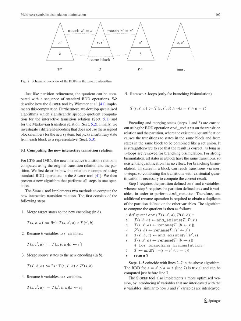
We present an alternative solution, which computes →∩ ≡ directly using a custom BDD algorithm. The inertalgorithm takes parameters T (s, s′) (T may contain othervariables ordered after s, s′) and two copies of P(s′, b): Ps

and Ps′ . The algorithm matches T and Ps on valuationsof variables s, and T and Ps′ on valuations of variables s′.See Algorithm 3, and also Fig. 2 for a schematic overview.When in the recursive call all valuations to s and s′ havebeen matched, with Ss, Ss′ ⊆ S the sets of states representedby these valuations, T is the set of actions that label thetransitions between states in Ss and Ss′ , Ps is the block thatcontains all Ss , and Ps′ is the block that contains all Ss′ .Then, if Ps �= Ps′ , the transitions are not inert and inertreturns False, removing the transition from T . Otherwise,T (which may still contain other variables ordered after s, s′,such as action labels) is returned.

5 Quotient computation

Computing the partition of the maximal bisimulation is onlythe first part of the minimisation process. Wemust also applythe partition to the original system, such that the blocks of thepartition become the states of the new transition system. Astraightforward conversion procedure encodes the new statesusing the block numbers assigned during partition refine-ment.

123


s, s s

b

s, ss

b

s = ss = s

T PsPs

Fig. 2 Schematic overview of the BDDs in the inert algorithm

Just like partition refinement, the quotient can be com-puted with a sequence of standard BDD operations. Wedescribe how the Sigref tool by Wimmer et al. [41] imple-ments this computation. Furthermore,wedevelop specialisedalgorithms which significantly speedup quotient computa-tion for the interactive transition relation (Sect. 5.1) andfor the Markovian transition relation (Sect. 5.2). Finally, weinvestigate a different encoding that does not use the assignedblock numbers for the new system, but picks an arbitrary statefrom each block as a representative (Sect. 5.3).

5.1 Computing the new interactive transition relation

For LTSs and IMCs, the new interactive transition relation iscomputed using the original transition relation and the par-tition. We first describe how this relation is computed usingstandard BDD operations in the Sigref tool [41]. We thenpresent a new algorithm that performs all steps in one oper-ation.

The Sigref tool implements two methods to compute thenew interactive transition relation. The first consists of thefollowing steps:

1. Merge target states to the new encoding (in b).

T (s, b, a) := ∃s′ : T (s, s′, a) ∧ P(s′, b)

2. Rename b variables to s′ variables.

T (s, s′, a) := T (s, b, a)[b ← s′]

3. Merge source states to the new encoding (in b).

T (s′, b, a) := ∃s : T (s, s′, a) ∧ P ′(s, b)

4. Rename b variables to s variables.

T (s, s′, a) := T (s′, b, a)[b ← s]

5. Remove τ -loops (only for branching bisimulation).

T (s, s′, a) := T (s, s′, a) ∧ ¬(s = s′ ∧ a = τ)

Encoding and merging states (steps 1 and 3) are carriedout using theBDDoperation and_exists on the transitionrelation and the partition, where the existential quantificationcauses the transitions to states in the same block and fromstates in the same block to be combined like a set union. Itis straightforward to see that the result is correct, as long asτ -loops are removed for branching bisimulation. For strongbisimulation, all states in a block have the same transitions, soexistential quantification has no effect. For branching bisim-ulation, all states in a block can reach transitions via inertτ -steps, so combining the transitions with existential quan-tification is necessary to compute the correct result.

Step 1 requires the partition defined on s′ and b variables,whereas step 3 requires the partition defined on s and b vari-ables, in order to perform and_exists. Therefore, oneadditional rename operation is required to obtain a duplicateof the partition defined on the other variables. The algorithmto compute the quotient is then as follows:

1 def quotient(T (s, s′, a), P(s′, b)):2 T (s, b, a) ← and_exists(T , P , s′)3 T (s, s′, a) ← rename(T , [b ← s′])4 P ′(s, b) ← rename(P , [s′ ← s])5 T (s′, b, a) ← and_exists(T , P ′, s)6 T (s, s′, a) ← rename(T , [b ← s])

# for branching bisimulation:7 T ← and(T , ¬(s = s′ ∧ a = τ))8 return T

Steps 1–5 coincide with lines 2–7 in the above algorithm.The BDD for s = s′ ∧ a = τ (line 7) is trivial and can becomputed just before line 7.

The Sigref tool also implements a more optimised ver-sion, by introducing b′ variables that are interleaved with theb variables, similar to how s and s′ variables are interleaved.

123


1. Merge target states to the new encoding (in b′).

T (s, b′, a) := ∃s′ : T (s, s′, a) ∧ P ′(s′, b′)


T (b, b′, a) := ∃s : T (s, a, b′) ∧ P ′′(s, b)

3. Rename b and b′ variables to s and s′ variables.

T (s, s′, a) := T (a, b, b′)[b ← s, b′ ← s′]


T (s, s′, a) := T (s, s′, a) ∧ ¬(s = s′ ∧ a = τ)

Since we use s′ and b variables for P , two rename opera-tions would be required to compute P ′(s′, b′) and P ′′(s, b).Instead, we perform this version as follows:


T (s, b, a) := ∃s′ : T (s, s′, a) ∧ P(s′, b)

2. Rename s and b variables to s′ and b′ variables.

T (s′, b′, a) := T (s, b, a)[s ← s′, b ← b′]


T (b, b′, a) := ∃s : T (s′, b′, a) ∧ P(s′, b)

4. Rename b and b′ variables to s and s′ variables.

T (s, s′, a) := T (b, b′, a)[b ← s, b′ ← s′]


T (s, s′, a) := T (s, s′, a) ∧ ¬(s = s′ ∧ a = τ)

This procedure avoids creating a copy of P by renaming.The implementation is then as follows:

1 def quotient(T (s, s′, a), P(s′, b)):2 T (s, b, a) ← and_exists(T , P , s′)3 T (s′, b′, a) ← rename(T , [s ← s′, b ← b′])4 T (b, b′, a) ← and_exists(T , P , s)5 T (s, s′, a) ← rename(T , [b ← s, b′ ← s′])

# for branching bisimulation:6 T ← and(T , ¬(s = s′ ∧ a = τ))7 return T

These algorithms still compute intermediate results thatcould be avoided by combining several steps into one opera-tion. For example, every rename operation essentially creates

1 def quotient(T , Ps , Ps′):2 if T = 0 : return 0

3 if result ← cache[(T ,Ps ,Ps′ )] : return result# interpret s′

i in Ps as si4 v = topVar (T , Ps , Ps′ )5 if v equals si for some i :

# match si in T with s′i in Ps

6 low ← quotient(Tsi=0, Pss′i=0, P

s′)

7 high ← quotient(Tsi=1, Pss′i=1, P

s′)

8 result ← or(low, high)9 elif v equals s′

i for some i :# match s′

i in T with s′i in Ps′

10 low ← quotient(Ts′i=0, Ps , Ps′s′i=0)

11 high ← quotient(Ts′i=1, Ps , Ps′s′i=1)

12 result ← or(low, high)13 else:

# remove inert τ-loops (branchingonly)

14 if Ps = Ps′ : T ← T ∧ ¬τ

# convert blocks Ps and Ps′

15 result ← makecube(Ps ,Ps′ ,T ))

16 cache[(T ,Ps ,Ps′ ] ← result17 return result

18 def makecube(Bs , Bs′ , A, V = s ∪ s′):19 if Bs = 0 ∨ Bs′ = 0 : return 020 if V = ∅ : return A21 v, V ← var(V), next(V)22 if v equals si for some i :23 low ← makecube(low(Bs),Bs′ ,A,V)

24 high ← makecube(high(Bs),Bs′ ,A,V)25 return lookupBDDnode(v, low, high)26 else:27 low ← makecube(Bs ,low(Bs′),A,V)

28 high ← makecube(Bs ,high(Bs′),A,V)29 return lookupBDDnode(v, low, high)

Algorithm4 Computes the quotient of a transition relationT accordingto the block assignments to current states (Ps ) and next states (Ps′ ).

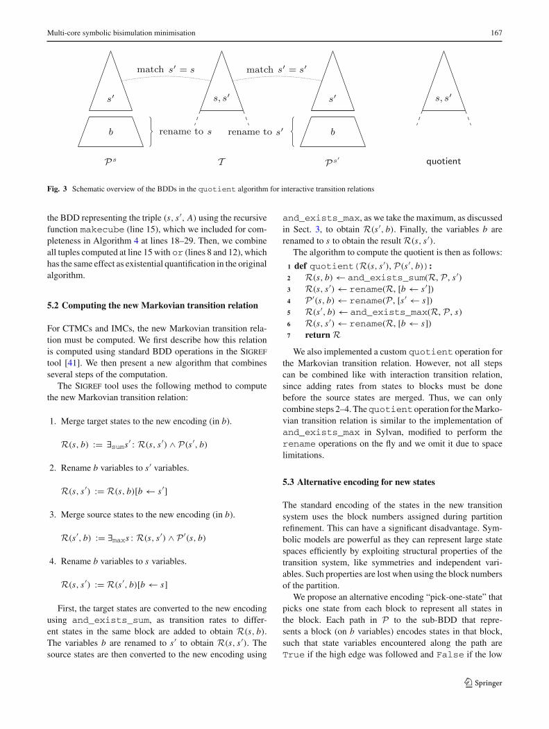
a duplicate of the original BDD, when most BDD nodesare affected by the renaming. Using a custom operation canmitigate this. Similar to the inert algorithm discussed inSect. 4.4, we implement the algorithm quotient that com-bines all steps of the above two algorithms. See Fig. 3 andAlgorithm 4. Note the similarities with Fig. 2 and Algo-rithm 3.

Like the inert operation, we evaluate and match thetransition relation with two copies of the partition (lines 1–12) and obtain the source block, the target block, and the setof actions at line 14–15. If we perform branching bisimula-tion and the source and target blocks are identical, we removethe τ transition from the obtained set of actions (line 14). Asthe two BDDs for the blocks are simple cubes that encodeexactly one block by assigning a value to each b variable, andT is the set of actions A, it is very straightforward to compute

123


s, s s

b

s, ss

b

s = ss = s

s s

T PsPs

Fig. 3 Schematic overview of the BDDs in the quotient algorithm for interactive transition relations

the BDD representing the triple (s, s′, A) using the recursivefunction makecube (line 15), which we included for com-pleteness in Algorithm 4 at lines 18–29. Then, we combineall tuples computed at line 15with or (lines 8 and 12), whichhas the same effect as existential quantification in the originalalgorithm.

5.2 Computing the new Markovian transition relation

For CTMCs and IMCs, the new Markovian transition rela-tion must be computed. We first describe how this relationis computed using standard BDD operations in the Sigreftool [41]. We then present a new algorithm that combinesseveral steps of the computation.

The Sigref tool uses the following method to computethe new Markovian transition relation:


R(s, b) := ∃sums′ : R(s, s′) ∧ P(s′, b)

2. Rename b variables to s′ variables.

R(s, s′) := R(s, b)[b ← s′]


R(s′, b) := ∃maxs : R(s, s′) ∧ P ′(s, b)

4. Rename b variables to s variables.

R(s, s′) := R(s′, b)[b ← s]

First, the target states are converted to the new encodingusing and_exists_sum, as transition rates to differ-ent states in the same block are added to obtain R(s, b).The variables b are renamed to s′ to obtain R(s, s′). Thesource states are then converted to the new encoding using

and_exists_max, as we take the maximum, as discussedin Sect. 3, to obtain R(s′, b). Finally, the variables b arerenamed to s to obtain the resultR(s, s′).

The algorithm to compute the quotient is then as follows:

1 def quotient(R(s, s′), P(s′, b)):2 R(s, b) ← and_exists_sum(R, P , s′)3 R(s, s′) ← rename(R, [b ← s′])4 P ′(s, b) ← rename(P , [s′ ← s])5 R(s′, b) ← and_exists_max(R, P , s)6 R(s, s′) ← rename(R, [b ← s])7 return R

We also implemented a custom quotient operation forthe Markovian transition relation. However, not all stepscan be combined like with interaction transition relation,since adding rates from states to blocks must be donebefore the source states are merged. Thus, we can onlycombine steps 2–4. Thequotientoperation for theMarko-vian transition relation is similar to the implementation ofand_exists_max in Sylvan, modified to perform therename operations on the fly and we omit it due to spacelimitations.

5.3 Alternative encoding for new states

The standard encoding of the states in the new transitionsystem uses the block numbers assigned during partitionrefinement. This can have a significant disadvantage. Sym-bolic models are powerful as they can represent large statespaces efficiently by exploiting structural properties of thetransition system, like symmetries and independent vari-ables. Such properties are lost when using the block numbersof the partition.

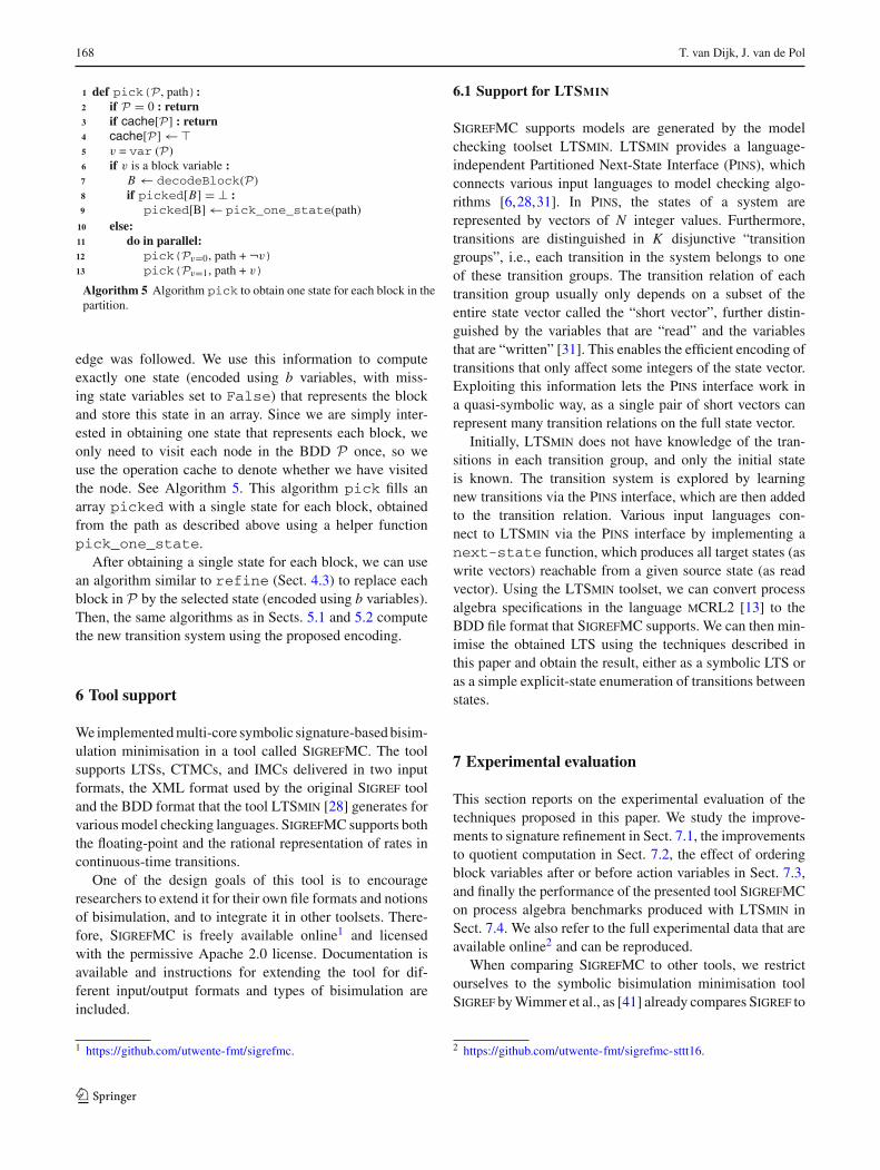
We propose an alternative encoding “pick-one-state” thatpicks one state from each block to represent all states inthe block. Each path in P to the sub-BDD that repre-sents a block (on b variables) encodes states in that block,such that state variables encountered along the path areTrue if the high edge was followed and False if the low

123


1 def pick(P , path):2 if P = 0 : return3 if cache[P] : return4 cache[P] ← �5 v = var (P)6 if v is a block variable :7 B ← decodeBlock(P)

8 if picked[B] = ⊥ :9 picked[B] ← pick_one_state(path)10 else:11 do in parallel:12 pick(Pv=0, path + ¬v)13 pick(Pv=1, path + v)

Algorithm 5 Algorithm pick to obtain one state for each block in thepartition.

edge was followed. We use this information to computeexactly one state (encoded using b variables, with miss-ing state variables set to False) that represents the blockand store this state in an array. Since we are simply inter-ested in obtaining one state that represents each block, weonly need to visit each node in the BDD P once, so weuse the operation cache to denote whether we have visitedthe node. See Algorithm 5. This algorithm pick fills anarray picked with a single state for each block, obtainedfrom the path as described above using a helper functionpick_one_state.

After obtaining a single state for each block, we can usean algorithm similar to refine (Sect. 4.3) to replace eachblock in P by the selected state (encoded using b variables).Then, the same algorithms as in Sects. 5.1 and 5.2 computethe new transition system using the proposed encoding.

6 Tool support

Weimplementedmulti-core symbolic signature-basedbisim-ulation minimisation in a tool called SigrefMC. The toolsupports LTSs, CTMCs, and IMCs delivered in two inputformats, the XML format used by the original Sigref tooland the BDD format that the tool LTSmin [28] generates forvariousmodel checking languages. SigrefMC supports boththe floating-point and the rational representation of rates incontinuous-time transitions.

One of the design goals of this tool is to encourageresearchers to extend it for their own file formats and notionsof bisimulation, and to integrate it in other toolsets. There-fore, SigrefMC is freely available online1 and licensedwith the permissive Apache 2.0 license. Documentation isavailable and instructions for extending the tool for dif-ferent input/output formats and types of bisimulation areincluded.

1 https://github.com/utwente-fmt/sigrefmc.

6.1 Support for LTSMIN

SigrefMC supports models are generated by the modelchecking toolset LTSmin. LTSmin provides a language-independent Partitioned Next-State Interface (Pins), whichconnects various input languages to model checking algo-rithms [6,28,31]. In Pins, the states of a system arerepresented by vectors of N integer values. Furthermore,transitions are distinguished in K disjunctive “transitiongroups”, i.e., each transition in the system belongs to oneof these transition groups. The transition relation of eachtransition group usually only depends on a subset of theentire state vector called the “short vector”, further distin-guished by the variables that are “read” and the variablesthat are “written” [31]. This enables the efficient encoding oftransitions that only affect some integers of the state vector.Exploiting this information lets the Pins interface work ina quasi-symbolic way, as a single pair of short vectors canrepresent many transition relations on the full state vector.

Initially, LTSmin does not have knowledge of the tran-sitions in each transition group, and only the initial stateis known. The transition system is explored by learningnew transitions via the Pins interface, which are then addedto the transition relation. Various input languages con-nect to LTSmin via the Pins interface by implementing anext-state function, which produces all target states (aswrite vectors) reachable from a given source state (as readvector). Using the LTSmin toolset, we can convert processalgebra specifications in the language mCRL2 [13] to theBDD file format that SigrefMC supports. We can then min-imise the obtained LTS using the techniques described inthis paper and obtain the result, either as a symbolic LTS oras a simple explicit-state enumeration of transitions betweenstates.

7 Experimental evaluation

This section reports on the experimental evaluation of thetechniques proposed in this paper. We study the improve-ments to signature refinement in Sect. 7.1, the improvementsto quotient computation in Sect. 7.2, the effect of orderingblock variables after or before action variables in Sect. 7.3,and finally the performance of the presented tool SigrefMCon process algebra benchmarks produced with LTSmin inSect. 7.4. We also refer to the full experimental data that areavailable online2 and can be reproduced.

When comparing SigrefMC to other tools, we restrictourselves to the symbolic bisimulation minimisation toolSigref byWimmer et al., as [41] already comparesSigref to

2 https://github.com/utwente-fmt/sigrefmc-sttt16.

123

https://github.com/utwente-fmt/sigrefmc

https://github.com/utwente-fmt/sigrefmc-sttt16


Table 1 Computation time in seconds for partition refinement on the benchmarks, comparing Sigref with SigrefMC

Model States Blocks Time Speedups

Tw T1 T48 Seq. Par. Total

LTS models (strong)

kanban03 1,024,240 85,356 92.16 10.09 0.88 9.14× 11.52× 105.29×kanban04 16,020,316 778,485 1410.66 148.15 11.37 9.52× 13.03× 124.06×kanban05 16,772,032 5,033,631 – 1284.86 73.57 – 17.47× –

kanban06 264,515,056 25,293,849 – – 2584.23 – – –

LTS models (branching)

kanban04 16,020,316 2785 8.47 0.52 0.24 16.39× 2.11× 34.60×kanban05 16,772,032 7366 34.11 1.48 0.43 22.98× 3.47× 79.81×kanban06 264,515,056 17,010 118.19 3.87 0.83 30.55× 4.65× 142.20×kanban07 268,430,272 35,456 387.16 8.83 1.66 43.86× 5.31× 232.71×kanban08 4,224,876,912 68,217 1091.67 17.91 2.98 60.96× 6.02× 366.72×kanban09 4,293,193,072 123,070 3186.48 34.23 5.51 93.10× 6.21× 578.59×

CTMC models

cycling-4 431,101 282,943 220.23 26.72 2.60 8.24× 10.29× 84.84×cycling-5 2,326,666 1,424,914 1249.23 170.28 19.42 7.34× 8.77× 64.34×fgf 80,616 38,639 71.62 8.86 0.88 8.08× 10.04× 81.20×p2p-5-6 230 336 750.29 26.96 2.99 27.83× 9.03× 251.24×p2p-6-5 230 266 248.17 9.49 1.21 26.15× 7.82× 204.47×p2p-7-5 235 336 2280.76 24.01 2.97 94.99× 8.08× 767.12×polling-16 1,572,864 98,304 792.82 118.50 10.18 6.69× 11.64× 77.85×polling-17 3,342,336 196,608 1739.01 303.65 22.58 5.73× 13.45× 77.03×polling-18 7,077,888 393,216 – 705.22 49.81 – 14.16× –

robot-020 31,160 30,780 28.15 3.21 0.60 8.78× 5.36× 47.04×robot-025 61,200 60,600 78.48 6.78 0.95 11.58× 7.11× 82.39×robot-030 106,140 105,270 174.30 12.26 1.47 14.21× 8.33× 118.44×

IMC models (strong)

ftwc01 2048 1133 1.26 1.14 0.2 1.11× 5.76× 6.38×ftwc02 32,768 16,797 154.55 102.07 15.85 1.51× 6.44× 9.75×

IMC models (branching)

ftwc01 2048 430 1.12 0.77 0.13 1.45× 6.07× 8.83×ftwc02 32,786 3886 152.9 50.39 4.89 3.03× 10.3× 31.26×

Each data point is an average of at least 15 runs. The timeout was 3600 s

other explicit-state and symbolic bisimulation minimisationtools.

7.1 Signature refinement

7.1.1 Design

To study the improvements to signature refinement thatwe present in this paper, we compared our results (usingthe skip list variant of refine) to Sigref 1.5 [40] forLTS and IMC models, and to a version of Sigref usedin [38] for CTMC models. For the CTMC models, weused Sigref with rational numbers provided by the GMP

library and SigrefMC with rational number support bySylvan. For the IMC models, version 1.5 of Sigref doesnot support the GMP library and the version used in [38]does not support IMCs. We used SigrefMC with float-ing points for a fairer comparison, but the tools give aslightly different number of blocks, due to the use of floatingpoints.

We restrict ourselves to the models presented in [38,41]and an IMC model that is part of the distribution of Sigref.These models have been generated from PRISM bench-marks using a custom version of the PRISM toolset [30].We refer to the literature for a description of thesemodels.

123


Fig. 4 Time per iteration for Sigref and SigrefMC (1 worker), andthe number of new blocks per iteration for strong bisimulation of thekanban04 LTS model

We perform experiments on the three tools using a 48-coremachine, containing 4 AMD OpteronTM 6168 processorswith 12 cores each. We measure the runtimes for the parti-tion refinement algorithm (excluding file-I/O) using Sigref,SigrefMCwith only 1worker, and SigrefMCwith 48work-ers.

Apart from the new refine and inert algorithms pre-sented in the current paper, there are several other differences.The first is that the original Sigref uses the CUDD imple-mentation of BDDs, while SigrefMC uses Sylvan, alongwith some extra BDD algorithms that avoid explicitly com-puting variable renaming of some BDDs. The second is thatSigref has several optimisations [40] that are not availablein SigrefMC.

7.1.2 Results

See Table 1 for the results of these experiments. These resultswere obtained by repeating each benchmark at least 15 times

and taking the average. The timeout was set to 3600 s. Thecolumn “States” shows the number of states before bisimu-lation minimisation and “Blocks” the number of equivalenceclasses after bisimulation minimisation. We show the wallclock time using Sigref (Tw), using SigrefMC with 1worker (T1) and using SigrefMCwith 48 workers (T48). Wecompute the sequential speedup Tw/T1, the parallel speedupT1/T48, and the total speedup Tw/T48.

Note that we obtained these results using the variableordering s, s′ < a < b; the other experiments are com-puted using the variable ordering s, s′ < b < a, as discussedbelow and in Sect. 4.2.

Due to space constraints, we do not include all results, butrestrict ourselves to larger models. We refer to the full exper-imental data that is available online. In the full set of results,excluding executions that take less than 1 s, SigrefMC isalways faster sequentially and always benefits from paral-lelism.

The results show a clear advantage for larger models. Oneinteresting result is for the p2p-7-5 model. This model isideal for symbolic bisimulation with a large number of states(235) and very few blocks after minimisation (336). For thismodel, our tool is 95× faster sequentially and has a parallelspeedup of 8×, resulting in a total speedup of 767×. Thebest parallel speedup of 17× was obtained for the kanban05model.

In almost all experiments, the signature computation dom-inates with 70–99% of the execution time sequentially. Weobserve that the refinement step sometimes benefits morefrom parallelism than signature computation, with speedupsup to 29.9×. We also find that reusing block numbers forstable blocks causes a major reduction in computation timetowards the end of the procedure. The kanban LTS mod-els and the larger polling CTMC models are an excellentcase study to demonstrate this. See Fig. 4. There is a clearcorrelation between the number of new blocks per iterationand the time per iteration for SigrefMC, while the time periteration for Sigref seems to correlate with the number ofblocks.

7.2 Quotient computation

7.2.1 Design

To study the different methods for quotient computation, weimplemented the methods described in Sects. 5.1 and 5.2:

– block-s: block encoding using standard operations– block: block encoding using specialised operations– pick: pick-one-state encoding, specialised operations

We computed the partition in SigrefMC using rationalnumbers for the Markovian transitions and with the variable

123


Table 2 Computation time in seconds for different implementations of quotient computation

block-s block pick

T1 T48 Sp. T1 T48 Sp. T1 T48 Sp.

LTS model (strong)

kanban03 24.64 1.5 16.42× 9.48 0.48 19.85× 6.72 0.35 19.08×kanban04 370.16 21.25 17.42× 129.19 7.84 16.47× 106.22 5.38 19.73×kanban05 – 175.92 – 1114.06 55.26 20.16× 740.53 33.80 21.91×

LTS model (branching)

kanban04 1.08 0.12 8.91× 0.20 0.03 6.67× 0.16 0.04 3.65×kanban05 3.48 0.33 10.71× 0.68 0.09 7.60× 0.51 0.10 5.05×kanban06 11.44 1.10 10.38× 1.90 0.27 6.95× 1.42 0.30 4.78×kanban07 29.94 3.02 9.93× 5.38 0.77 7.00× 3.17 0.64 4.93×kanban08 110.47 8.34 13.24× 11.52 1.52 7.56× 7.01 1.29 5.44×kanban09 200.44 18.77 10.68× 27.05 3.83 7.06× 14.21 2.74 5.19×

CTMC model

cycling-4 170.2 9.51 17.91× 40.22 3.05 13.21× 59.51 3.32 17.90×cycling-5 1039.17 55.52 18.72× 231.25 14.01 16.50× 294.15 13.48 21.83×fgf 17.77 1.64 10.83× 6.12 0.61 9.99× 7.42 0.73 10.20×kanban-3 19.32 1.5 12.87× 6.4 0.58 11.07× 7.04 0.49 14.26×kanban-4 285.52 14.72 19.40× 81.57 4.67 17.48× 104.65 5.08 20.60×p2p-5-6 22.1 2.34 9.45× 9.66 1.12 8.63× 10.25 1.41 7.29×p2p-6-5 7.45 0.91 8.17× 3.41 0.45 7.64× 3.67 0.55 6.71×p2p-7-5 17.55 2.02 8.71× 8.84 1.05 8.39× 9.26 1.19 7.79×polling-16 176.47 8.74 20.20× 95.33 4.83 19.76× 66.25 4.49 14.75×polling-17 416.17 20.65 20.16× 223.11 11.51 19.39× 161.74 10.02 16.14×polling-18 1063.13 53.38 19.92× 542.02 26.43 20.51× 359.49 21.68 16.58×robot-020 3.47 0.27 12.68× 1.72 0.16 10.83× 1.55 0.12 12.57×robot-025 6.97 0.54 13.00× 3.39 0.32 10.66× 2.91 0.25 11.83×robot-030 12.36 1.03 12.04× 5.84 0.53 10.98× 4.81 0.41 11.78×

IMC model (strong)

ftwc01 1.62 0.16 10.06× 1.69 0.14 12.22× 0.96 0.08 11.98×ftwc02 208.89 20.78 10.05× 370.16 36.65 10.10× 301.88 15.34 19.68×

IMC model (branching)

ftwc01 0.36 0.05 6.99× 0.3 0.03 9.00× 0.19 0.03 6.83×ftwc02 17.13 1.72 9.98× 15.73 1.45 10.86× 5.24 0.49 10.77×

Each data point is an average of at least 12 runs. The timeout was 1200 s to compute the partition and the quotient

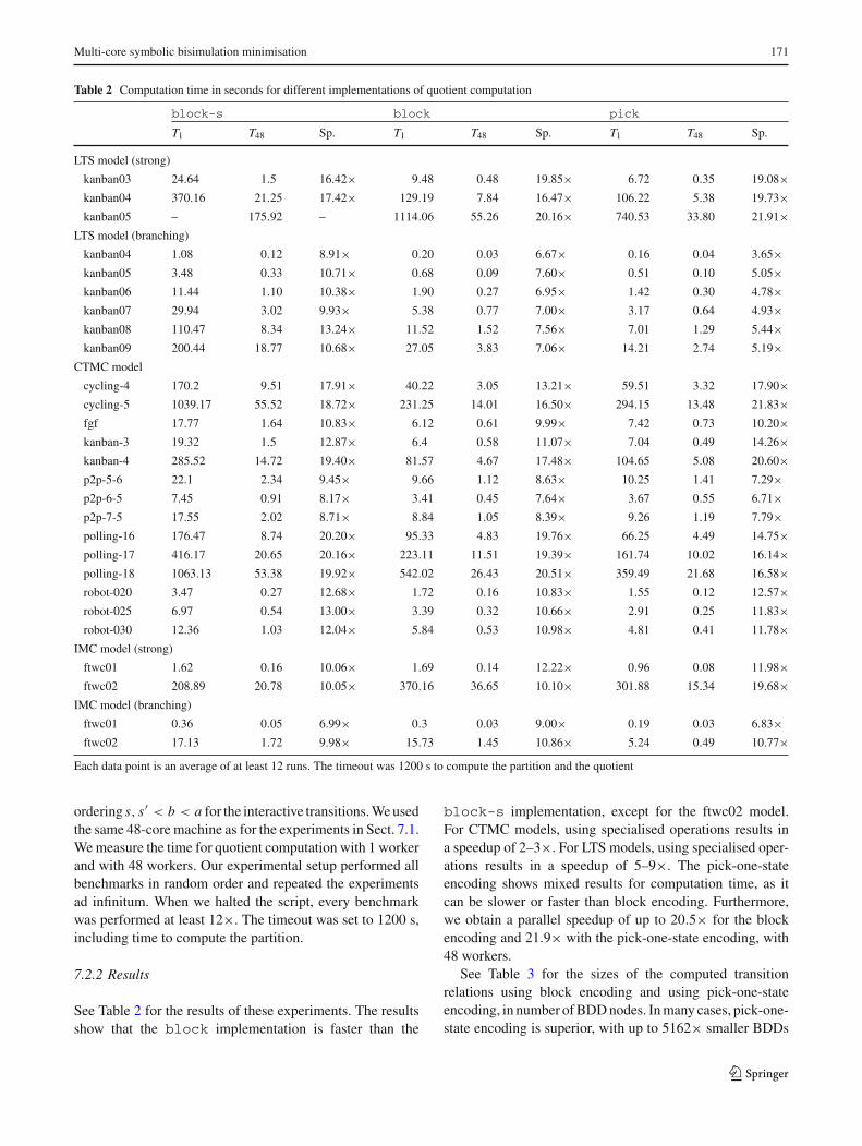
ordering s, s′ < b < a for the interactive transitions.Weusedthe same 48-core machine as for the experiments in Sect. 7.1.Wemeasure the time for quotient computation with 1 workerand with 48 workers. Our experimental setup performed allbenchmarks in random order and repeated the experimentsad infinitum. When we halted the script, every benchmarkwas performed at least 12×. The timeout was set to 1200 s,including time to compute the partition.

7.2.2 Results

See Table 2 for the results of these experiments. The resultsshow that the block implementation is faster than the

block-s implementation, except for the ftwc02 model.For CTMC models, using specialised operations results ina speedup of 2–3×. For LTS models, using specialised oper-ations results in a speedup of 5–9×. The pick-one-stateencoding shows mixed results for computation time, as itcan be slower or faster than block encoding. Furthermore,we obtain a parallel speedup of up to 20.5× for the blockencoding and 21.9× with the pick-one-state encoding, with48 workers.

See Table 3 for the sizes of the computed transitionrelations using block encoding and using pick-one-stateencoding, in number ofBDDnodes. Inmany cases, pick-one-state encoding is superior, with up to 5162× smaller BDDs

123


Table 3 Number of BDDnodes for the transition relation after quotientcomputation, for the block number encoding and the pick-one-stateencoding

block pick factor

LTS (strong)

kanban03 710,359 6137 115.75×kanban04 6,553,843 14,599 448.92×kanban05 43,901,839 27,600 1590.65×

LTS (branching)

kanban04 17,510 1081 16.20×kanban05 47,920 1259 38.06×kanban06 110,069 1944 56.62×kanban07 233,902 1999 117.01×kanban08 442,890 2838 156.06×kanban09 800,649 3388 236.32×

IMC (strong)

ftwc01 47,859 660 72.51×ftwc02 5,669,528 1208 4693.32×

IMC (branching)

ftwc01 2137 285 7.50×ftwc02 49,093 413 118.87×ftwc03 1,236,052 541 2284.75×

CTMC

cycling-4 1,869,641 185,824 10.06×cycling-5 8,960,365 430,936 20.79×fgf 422,954 38,452 11.00×kanban-3 354,774 2473 143.46×kanban-4 3,032,327 4899 618.97×p2p-5-6 1513 2635 0.57×p2p-6-5 1039 2151 0.48×p2p-7-5 1428 3057 0.47×polling-16 715,145 494 1447.66×polling-17 1,442,013 529 2725.92×polling-18 2,901,462 562 5162.74×robot-020 148,385 3790 39.15×robot-025 260,514 4785 54.44×robot-030 411,624 5512 74.68×

for the polling models. For the p2p models, block encodingis superior, likely due to the small number of blocks afterbisimulation minimisation.

7.3 Variable ordering

7.3.1 Design

As discussed in Sect. 4.2, we can choose to order blockvariables b before or after action variables a in the variableordering of theBDDs. To compare the ordering s, s′ < a < b

and s, s′ < b < a, we compare signature refinement andquotient computation for the kanban LTS models.

We expect that in general ordering b before a is the bestchoice. If we have a variables before b variables, then it isguaranteed that all BDD nodes on a variables are recreatedwhen we compute signatures for partition refinement andwhen we compute the quotient, whereas they may be reusedif a variables are last in the ordering.

7.3.2 Results

See Table 4 for the results of this experiment. All data pointsare computed with at least 5 runs. We computed the quo-tient using the pick-one-state algorithm. We see that in mostcases the ordering with b before a is superior. We observea stronger effect for partition refinement than for quotientcomputation. The surprising exception is quotient computa-tion of the kanban04 model with strong bisimulation, wherethe ordering with a before b is slightly better, although thetotal time still favours ordering b before a.

7.4 Process algebra experiments

7.4.1 Design

As described in Sect. 6.1, we extended SigrefMC withsupport for BDDs produced by the model checking toolsetLTSmin from process algebra models specified in themCRL2 specification language.

We first took a number of communication protocols fromthe mCRL2 example directory, in particular the boundedretransmission protocol (BRP) and the Sliding Window Pro-tocol (SWP). We made them parametric in the number ofdata elements, number of retries, window size, etc. We alsoinclude a number of distributed algorithms. We ported theprobabilistic leader election protocols [3], based on Dolev–Klawe–Rodeh and Franklin, fromμCRL tomCRL2. We alsoincluded Hesselink’s hardware register [27]. Finally, we alsoincluded an industrial case study: Workload ManagementSystem of the computation grid at the Large Hadron ColliderLHC (CERN), specified in [36].

This leads to the following specifications:

– SWP_m_n: the Sliding Window Protocol [1] on mdata items, with window size n. This specifies a one-directional version of the sliding window protocol. nsubsequent data items can be sent and acknowledged inarbitrary order. This requires sequence numbers mod-ulo 2n. Its external behaviour is equivalent to a 2n-placebuffer.

– BRP_m_�_n: the bounded retransmission protocol [24]on m data items, sending a list of length � and with n

123


Table 4 Computation time in seconds on the LTS benchmarks, with the variable orders s, s′ < a < b and s, s′ < b < a, for both partitionrefinement and quotient computation, with 1 worker and 48 workers

Model (bisimulation) Partition, 1 worker Partition, 48 workers Quotient, 1 worker Quotient, 48 workers

a < b b < a a < b b < a a < b b < a a < b b < a

kanban03 (strong) 8.69 6.86 1.10 1.01 6.83 6.72 0.36 0.35

kanban04 (strong) 127.54 102.11 13.86 11.66 98.12 106.22 4.25 5.38

kanban05 (strong) 1211.20 1076.17 99.63 95.09 854.62 740.53 34.17 33.80

kanban04 (branching) 0.40 0.38 0.22 0.23 0.16 0.16 0.04 0.04






retries. This protocol extends the ABP, but gives up aftern retries. The status of the transmission is returned toboth the sender and the receiver. The external behaviouris a bit complicated, since the sender cannot distinguishif the last data element or the last acknowledgement gotlost.

– DKR_n: randomised variant [3] of Dolev–Klawe–Rod-eh’s [22] Leader Election Protocol on a uni-directionalring with n anonymous partners. Several rounds may beneeded when partners choose the same identity. The pro-tocol is based on hop counters and on an alternating bit todistinguish subsequent rounds. The external behaviour isequivalent to a single leader action.

– Franklin_n_m: randomised variant [3] of Franklin’sLeader Election Protocol [23], but now on a bidirectionalringwith n partners, usingm ≤ n different identities. Theexternal behaviour is again equivalent to a single leaderaction.

– Hesselink_n: Hesselink’s handshake register [27], con-structed from four safe registers and four Boolean atomicregisters, modelled in mCRL2 by Groote, and used forexperimentation in [34].

– WMS: this models the Workload Management Systemof the DIRAC (Distributed Infrastructure with RemoteAgent Control) for the Large Hadron Collider experi-ments at CERN, as described in [36].

We used the following toolchain to generate input files forSigrefMC:

1. mcrl22lps -Dfvn from the mCRL2 toolset to gen-erate LPS files from the specifications

2. lps2lts-sym --vset=lddmc from the LTSmintoolset to generate the transition systems in LDD formatfrom the LPS files

3. ldd2bdd from the LTSmin toolset to convert the tran-sition systems from LDDs to BDDs

To evaluate SigrefMC on these models, we performedthe same experiments as in Sect. 7.2.

Wemeasure the time for partition refinement and quotientcomputation with 1 worker and with 48 workers. Our exper-imental setup performed all benchmarks in random orderand repeated the experiments ad infinitum. When we haltedthe script, every benchmark was performed at least 6×. Thetimeout was set to 1200 s for the entire program, i.e., partitionrefinement and quotient computation.

7.4.2 Results

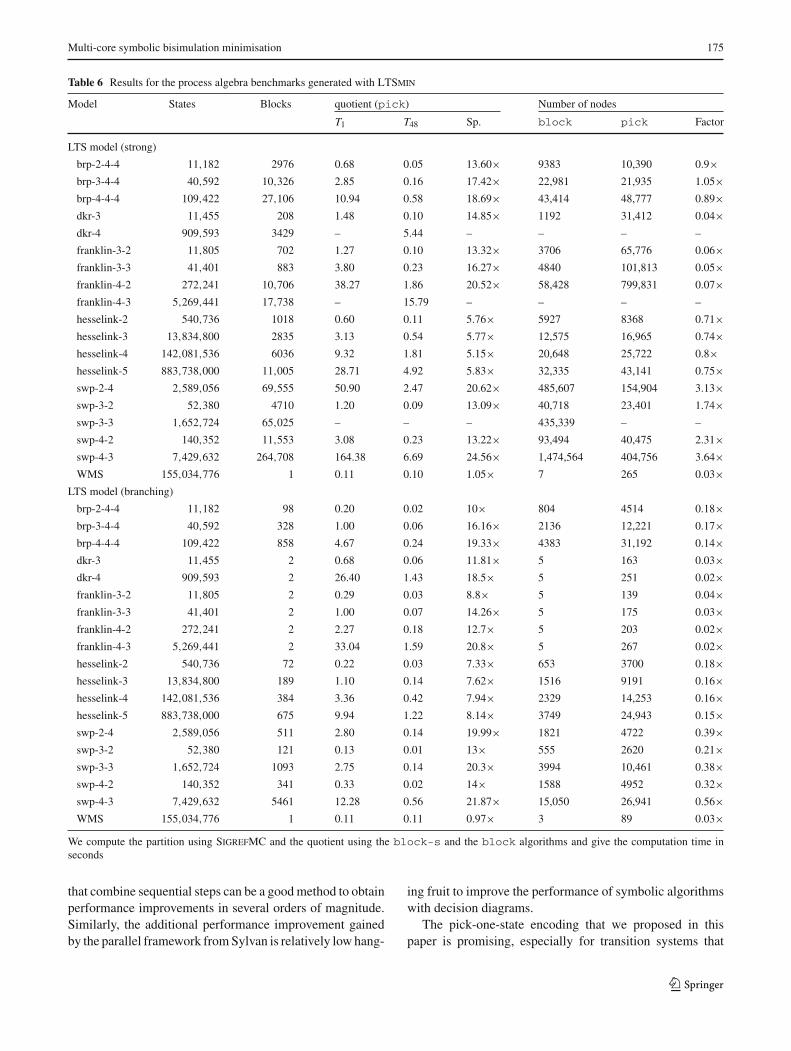
The results are summarised in Tables 5 and 6. We do notinclude all results to conserve space; all results from theexperiments are available online.

It is interesting to see that both strong andbranchingbisim-ulation result in huge reductions. We see clear benefit fromparallel processing, with speedups of up to 24.7× for sig-nature refinement and up to 24.5× for quotient computation(block encoding)

The pick-one-state encoding does not work so well here.Probably because the number of blocks is low; also the statevectors are relatively long. For a few models, the pick-one-state encoding works relatively well; these are models thathave a high number of blocks.

8 Conclusions

Originally,we intended to investigate parallelism in symbolicbisimulation minimisation. To our surprise, we obtained amuchhigher sequential speedupusing specialisedBDDoper-ations, as demonstrated by the results in Table 1 and Fig. 4.

123


Table 5 Results for the process algebra benchmarks generated with LTSmin

Model States Blocks Signature refinement Quotient (block-s) Quotient (block)

T1 T48 Sp. T1 T48 Sp. T1 T48 Sp.

LTS model (strong)

brp-2-4-4 11,182 2976 3.92 0.35 11.23× 1.32 0.43 3.08× 0.57 0.04 13.26×brp-3-4-4 40,592 10,326 13.50 0.92 14.75× 5.30 0.63 8.48× 2.45 0.14 17.53×brp-4-4-4 109,422 27,106 38.91 2.23 17.43× 18.03 1.49 12.10× 9.84 0.52 18.93×dkr-3 11,455 208 7.64 0.54 14.05× 3.64 0.38 9.57× 1.31 0.09 14.50×dkr-4 909,593 3429 – 115.28 – – 25.86 – – 4.99 –

franklin-3-2 11,805 702 7.15 0.47 15.21× 4.71 0.42 11.12× 0.99 0.07 13.55×franklin-3-3 41,401 883 24 1.24 19.40× 16.25 1.05 15.52× 3.13 0.19 16.46×franklin-4-2 272,241 10,706 330.56 14.67 22.53× 204.68 9.65 21.21× 28.04 1.43 19.63×franklin-4-3 5,269,441 17,738 – 441.56 – – 115.02 – – 13.87 –

hesselink-2 540,736 1018 3.49 0.34 10.30× 1.96 0.30 6.60× 0.43 0.07 5.94×hesselink-3 13,834,800 2835 17.70 1.42 12.50× 16.16 1.57 10.27× 2.33 0.35 6.58×hesselink-4 142,081,536 6036 51.41 3.56 14.44× 66.71 5.37 12.43× 7.01 1.21 5.78×hesselink-5 883,738,000 11,005 179.85 12.61 14.26× 313.42 25.40 12.34× 22.32 3.64 6.14×swp-2-4 2,589,056 69,555 267.46 11.33 23.60× 258.66 13.40 19.30× 30.78 1.39 22.21×swp-3-2 52,380 4710 4.12 0.25 16.45× 4.98 0.39 12.71× 0.73 0.05 14.57×swp-3-3 1,652,724 65,025 142.60 6.13 23.26× 188.10 9.60 19.60× 24.89 1.11 22.39×swp-4-2 140,352 11,553 9.77 0.54 18.02× 13.18 0.98 13.40× 1.96 0.12 16.10×swp-4-3 7,429,632 – 630.73 25.92 24.34× – 47.05 – 111.69 4.55 24.56×WMS 155,034,776 1 0.12 0.02 4.91× 0.11 0.20 0.56× 0.10 0.13 0.79×


brp-2-4-4 11,182 98 3.63 0.36 10.11× 0.28 0.10 2.67× 0.18 0.02 7.71×brp-3-4-4 40,592 328 13.78 0.98 14.08× 0.28 0.10 2.67× 0.18 0.02 7.71×brp-4-4-4 109,422 858 39.71 2.16 18.38× 4.04 0.48 8.47× 4.52 0.23 19.64×dkr-3 11,455 2 4.46 0.33 13.39× 0.94 0.38 2.47× 0.63 0.05 11.79×dkr-4 909,593 2 349.24 15.31 22.81× 45.30 10.60 4.27× 25.73 1.37 18.82×franklin-3-2 11,805 2 3.62 0.29 12.58× 0.53 0.35 1.50× 0.28 0.04 6.64×franklin-3-3 41,401 2 11.94 0.66 17.96× 1.80 0.47 3.88× 0.95 0.07 13.55×franklin-4-2 272,241 2 50.97 2.40 21.28× 4.76 1.76 2.71× 2.19 0.18 12.28×franklin-4-3 5,269,441 2 807.72 32.69 24.71× 67.70 22.37 3.03× 31.94 1.56 20.52×hesselink-2 540,736 72 7.64 0.79 9.71× 0.73 0.15 4.80× 0.19 0.03 6.33×hesselink-3 13,834,800 189 37.10 2.76 13.46× 5.88 0.66 8.86× 0.94 0.13 7.36×hesselink-4 142,081,536 384 114.37 7.98 14.33× 26.66 2.05 12.97× 2.79 0.38 7.44×hesselink-5 883,738,000 675 351.69 23.93 14.70× 102.95 7.38 13.95× 8.33 1.11 7.49×swp-2-4 2,589,056 511 116.16 5.08 22.88× 20.58 1.33 15.53× 2.32 0.13 18.09×swp-3-2 52,380 121 4.41 0.31 14.07× 0.67 0.09 7.76× 0.11 0.01 11.00×swp-3-3 1,652,724 1093 135.99 6.21 21.88× 18.35 1.16 15.84× 2.34 0.12 19.51×swp-4-2 140,352 341 8.13 0.46 17.85× 1.96 0.34 5.74× 0.28 0.03 11.13×swp-4-3 7,429,632 5461 420.09 17.13 24.52× 99.64 5.42 18.38× 10.59 0.49 21.68×WMS 155,034,776 1 0.36 0.22 1.66× 0.11 0.22 0.51× 0.10 0.11 0.93×

We compute the partition using SigrefMC and the quotient using the block-s and the block algorithms and give the computation time inseconds

The specialised BDD operations offer a clear advantagesequentially and the integration with Sylvan results in decentparallel speedups. Our best result had a total speedup of767×. By also using specialisedBDDoperations for quotient

computation, we demonstrated performance improvementsin 2–10× over using standard BDD operations.

The success of this approach suggests that for applica-tions that involve decision diagrams, specialised operations

123


Table 6 Results for the process algebra benchmarks generated with LTSmin

Model States Blocks quotient (pick) Number of nodes

T1 T48 Sp. block pick Factor

LTS model (strong)

brp-2-4-4 11,182 2976 0.68 0.05 13.60× 9383 10,390 0.9×brp-3-4-4 40,592 10,326 2.85 0.16 17.42× 22,981 21,935 1.05×brp-4-4-4 109,422 27,106 10.94 0.58 18.69× 43,414 48,777 0.89×dkr-3 11,455 208 1.48 0.10 14.85× 1192 31,412 0.04×dkr-4 909,593 3429 – 5.44 – – – –

franklin-3-2 11,805 702 1.27 0.10 13.32× 3706 65,776 0.06×franklin-3-3 41,401 883 3.80 0.23 16.27× 4840 101,813 0.05×franklin-4-2 272,241 10,706 38.27 1.86 20.52× 58,428 799,831 0.07×franklin-4-3 5,269,441 17,738 – 15.79 – – – –

hesselink-2 540,736 1018 0.60 0.11 5.76× 5927 8368 0.71×hesselink-3 13,834,800 2835 3.13 0.54 5.77× 12,575 16,965 0.74×hesselink-4 142,081,536 6036 9.32 1.81 5.15× 20,648 25,722 0.8×hesselink-5 883,738,000 11,005 28.71 4.92 5.83× 32,335 43,141 0.75×swp-2-4 2,589,056 69,555 50.90 2.47 20.62× 485,607 154,904 3.13×swp-3-2 52,380 4710 1.20 0.09 13.09× 40,718 23,401 1.74×swp-3-3 1,652,724 65,025 – – – 435,339 – –

swp-4-2 140,352 11,553 3.08 0.23 13.22× 93,494 40,475 2.31×swp-4-3 7,429,632 264,708 164.38 6.69 24.56× 1,474,564 404,756 3.64×WMS 155,034,776 1 0.11 0.10 1.05× 7 265 0.03×


brp-2-4-4 11,182 98 0.20 0.02 10× 804 4514 0.18×brp-3-4-4 40,592 328 1.00 0.06 16.16× 2136 12,221 0.17×brp-4-4-4 109,422 858 4.67 0.24 19.33× 4383 31,192 0.14×dkr-3 11,455 2 0.68 0.06 11.81× 5 163 0.03×dkr-4 909,593 2 26.40 1.43 18.5× 5 251 0.02×franklin-3-2 11,805 2 0.29 0.03 8.8× 5 139 0.04×franklin-3-3 41,401 2 1.00 0.07 14.26× 5 175 0.03×franklin-4-2 272,241 2 2.27 0.18 12.7× 5 203 0.02×franklin-4-3 5,269,441 2 33.04 1.59 20.8× 5 267 0.02×hesselink-2 540,736 72 0.22 0.03 7.33× 653 3700 0.18×hesselink-3 13,834,800 189 1.10 0.14 7.62× 1516 9191 0.16×hesselink-4 142,081,536 384 3.36 0.42 7.94× 2329 14,253 0.16×hesselink-5 883,738,000 675 9.94 1.22 8.14× 3749 24,943 0.15×swp-2-4 2,589,056 511 2.80 0.14 19.99× 1821 4722 0.39×swp-3-2 52,380 121 0.13 0.01 13× 555 2620 0.21×swp-3-3 1,652,724 1093 2.75 0.14 20.3× 3994 10,461 0.38×swp-4-2 140,352 341 0.33 0.02 14× 1588 4952 0.32×swp-4-3 7,429,632 5461 12.28 0.56 21.87× 15,050 26,941 0.56×WMS 155,034,776 1 0.11 0.11 0.97× 3 89 0.03×

We compute the partition using SigrefMC and the quotient using the block-s and the block algorithms and give the computation time inseconds

that combine sequential steps can be a goodmethod to obtainperformance improvements in several orders of magnitude.Similarly, the additional performance improvement gainedby the parallel framework fromSylvan is relatively low hang-

ing fruit to improve the performance of symbolic algorithmswith decision diagrams.

The pick-one-state encoding that we proposed in thispaper is promising, especially for transition systems that

123


are still relatively large after bisimulation minimisation. Theimplementation discussed here just picked an arbitrary state;we expect that better heuristics may be developed in thefuture.

A limitation of this study is that we only measured theperformance on the benchmarks that were used in [38,40]and on several benchmarks from the mCRL2 distribution.

Acknowledgements Openaccess fundingprovidedby JohannesKeplerUniversity Linz.

Open Access This article is distributed under the terms of the CreativeCommons Attribution 4.0 International License (http://creativecommons.org/licenses/by/4.0/), which permits unrestricted use, distribution,and reproduction in any medium, provided you give appropriate creditto the original author(s) and the source, provide a link to the CreativeCommons license, and indicate if changes were made.

References

1. Badban, B., Fokkink, W., Groote, J.F., Pang, J., van de Pol, J.: Ver-ification of a sliding window protocol in μCRL and PVS. FormalAsp. Comput. 17(3), 342–388 (2005)

2. Bahar, R.I., Frohm, E.A., Gaona, C.M., Hachtel, G.D., Macii, E.,Pardo, A., Somenzi, F.: Algebraic decision diagrams and theirapplications. ICCAD 1993, 188–191 (1993)

3. Bakhshi, R., Fokkink, W., Pang, J., van de Pol, J.: Leader electionin anonymous rings: Franklin goes probabilistic. In: Ausiello, G.,Karhumäki, J., Mauri, G., Ong, C.L. (eds.) TCS’08, IFIP, vol. 273,pp. 57–72. Springer, Berlin (2008)

4. Blom, S., Haverkort, B.R., Kuntz, M., van de Pol, J.: DistributedMarkovian bisimulation reduction aimed at CSL model checking.ENTCS 220(2), 35–50 (2008)

5. Blom, S., Orzan, S.: Distributed branching bisimulation reductionof state spaces. ENTCS 89(1), 99–113 (2003)

6. Blom, S., van de Pol, J., Weber, M.: LTSmin: distributed andsymbolic reachability. In: CAV, LNCS, vol. 6174, pp. 354–359.Springer (2010)

7. Blumofe, R.D.: Scheduling multithreaded computations by workstealing. In: FOCS, pp. 356–368. IEEE Computer Society (1994)

8. Bouali, A., de Simone,R.: Symbolic bisimulationminimisation. In:Computer Aided Verification, 4th International Workshop, LNCS,vol. 663, pp. 96–108. Springer (1992)

9. Brace, K.S., Rudell, R.L., Bryant, R.E.: Efficient implementationof a BDD package. In: DAC, pp. 40–45 (1990)

10. Bryant, R.E.: Graph-based algorithms for Boolean functionmanip-ulation. IEEE Trans. Comput. C–35(8), 677–691 (1986)

11. Burch, J., Clarke, E., Long, D., McMillan, K., Dill, D.: Symbolicmodel checking for sequential circuit verification. IEEE Trans.Comput. Aided Des. Integr. Circuits Syst. 13(4), 401–424 (1994)

12. Clarke, E.M.,McMillan, K.L., Zhao, X., Fujita,M., Yang, J.: Spec-tral transforms for large Boolean functions with applications totechnology mapping. In: DAC, pp. 54–60 (1993)

13. Cranen, S., Groote, J.F., Keiren, J.J.A., Stappers, F.P.M., de Vink,E.P.,Wesselink,W.,Willemse, T.A.C.: An overview of themCRL2toolset and its recent advances. In: TACAS, LNCS, vol. 7795, pp.199–213. Springer (2013)

14. De Nicola, R., Vaandrager, F.W.: Three logics for branching bisim-ulation. J. ACM 42(2), 458–487 (1995)

15. Derisavi, S.: A symbolic algorithm for optimalMarkov chain lump-ing. TACAS 2007, 139–154 (2007)

16. Derisavi, S.: Signature-based symbolic algorithm for optimalMarkov chain lumping. In: QEST 2007, pp. 141–150. IEEE Com-puter Society (2007)

17. van Dijk, T.: Sylvan: multi-core decision diagrams. Ph.D. thesis,University of Twente (2016)

18. van Dijk, T., Laarman, A., van de Pol, J.: Multi-core BDD opera-tions for symbolic reachability. ENTCS 296, 127–143 (2013)

19. vanDijk, T., vandePol, J.: Lace: non-blocking split deque forwork-stealing. In: MuCoCoS, LNCS, vol. 8806, pp. 206–217. Springer(2014)

20. van Dijk, T., van de Pol, J.: Sylvan: multi-core decision diagrams.In: TACAS, LNCS, vol. 9035, pp. 677–691. Springer (2015)

21. van Dijk, T., van de Pol, J.: Multi-core symbolic bisimulation min-imisation. In: TACAS, LNCS, vol. 9636, pp. 332–348. Springer(2016)

22. Dolev, D., Klawe, M.M., Rodeh, M.: An o(n log n) unidirectionaldistributed algorithm for extrema finding in a circle. J. Algorithms3(3), 245–260 (1982)

23. Franklin, W.R.: On an improved algorithm for decentralizedextrema finding in circular configurations of processors. Commun.ACM 25(5), 336–337 (1982)

24. Groote, J.F., van de Pol, J.: A bounded retransmission protocol forlarge data packets. In: Wirsing, M., Nivat, M. (eds.) AMAST’96,LNCS 1101, pp. 536–550. Springer, Berlin (1996)

25. Hermanns, H.: Interactive Markov Chains: The Quest for Quan-tified Quality, Lecture Notes in Computer Science, vol. 2428.Springer, Berlin (2002)

26. Hermanns, H., Katoen, J.: The how and why of interactive Markovchains. In: FMCO’09, LNCS 6286, pp. 311–337. Springer (2009)

27. Hesselink, W.H.: Invariants for the construction of a handshakeregister. Inf. Process. Lett. 68(4), 173–177 (1998)

28. Kant, G., Laarman, A., Meijer, J., van de Pol, J., Blom, S.,van Dijk, T.: LTSmin: high-performance language-independentmodel checking. In: TACAS 2015, LNCS, vol. 9035, pp. 692–707.Springer (2015)

29. Kulakowski, K.: Concurrent bisimulation algorithm. CoRR.arXiv:1311.7635 (2013)

30. Kwiatkowska, M.Z., Norman, G., Parker, D.: PRISM 4.0: verifica-tion of probabilistic real-time systems. In: CAV, LNCS, vol. 6806,pp. 585–591. Springer (2011)

31. Meijer, J., Kant, G., Blom, S., van de Pol, J.: Read, write and copydependencies for symbolic model checking. In: Yahav, E. (ed.)HVC, LNCS, vol. 8855, pp. 204–219. Springer, Berlin (2014)

32. Mumme, M., Ciardo, G.: An efficient fully symbolic bisimulationalgorithm for non-deterministic systems. Int. J. Found. Comput.Sci. 24(2), 263–282 (2013)

33. Paige, R., Tarjan, R.E.: Three partition refinement algorithms.SIAM J. Comput. 16(6), 973–989 (1987)

34. van de Pol, J., Timmer,M.: State space reduction of linear processesusing control flow reconstruction. In: Liu, Z., Ravn, A.P. (eds.)ATVA’09, LNCS, vol. 5799, pp. 54–68. Springer, Berlin (2009)

35. Pugh, W.: Skip lists: a probabilistic alternative to balanced trees.Commun. ACM 33(6), 668–676 (1990)

36. Remenska, D., Willemse, T.A.C., Verstoep, K., Fokkink, W., Tem-plon, J., Bal, H.E.: Using model checking to analyze the systembehavior of the LHC production grid. In: CCGrid’12, pp. 335–343.IEEE Computer Society (2012)

37. Wijs,A.:GPUaccelerated strong and branching bisimilarity check-ing. TACAS 2015, 368–383 (2015)

38. Wimmer, R., Becker, B.: Correctness issues of symbolic bisimula-tion computation for Markov chains. In: MMB&DFT, LNCS, vol.5987, pp. 287–301. Springer (2010)

39. Wimmer, R., Derisavi, S., Hermanns,H.: Symbolic partition refine-ment with automatic balancing of time and space. Perform. Eval.67(9), 816–836 (2010)

123

http://creativecommons.org/licenses/by/4.0/

http://creativecommons.org/licenses/by/4.0/

http://arxiv.org/abs/1311.7635


40. Wimmer, R., Herbstritt, M., Becker, B.: Optimization techniquesfor BDD-based bisimulation computation. In: 17th GLSVLSI, pp.405–410. ACM (2007)

41. Wimmer, R., Herbstritt, M., Hermanns, H., Strampp, K., Becker,B.: Sigref—a symbolic bisimulation tool box. In: ATVA, LNCS,vol. 4218, pp. 477–492. Springer (2006)

42. Wimmer, R., Hermanns, H., Herbstritt, M., Becker, B.: Towardssymbolic stochastic aggregation. Technical Report, SFB/TR 14AVACS (2007)

123

multi-core symbolic bisimulation minimisation · int j softw tools technol transfer (2018)...

Documents