multi-camera intelligent space for a robust, fast and easy ... · 6 wireless localisation with...
TRANSCRIPT

Multi-camera intelligent space for arobust, fast and easy deployment of
proactive robots in complex anddynamic environments
Adrián Canedo Rodríguez
DEPARTAMENTO DE ELECTRÓNICA E COMPUTACIÓN
CENTRO SINGULAR DE INVESTIGACIÓN EN TECNOLOXÍAS DA INFORMACIÓN
UNIVERSIDADE DE SANTIAGO DE COMPOSTELA


UNIVERSIDADE DE SANTIAGO DE COMPOSTELA
Centro Singular de Investigación en Tecnoloxías da InformaciónDepartamento de Electrónica e Computación
Thesis
MULTI-CAMERA INTELLIGENT SPACE FOR A ROBUST, FASTAND EASY DEPLOYMENT OF PROACTIVE ROBOTS IN
COMPLEX AND DYNAMIC ENVIRONMENTS
Author:Adrián Canedo Rodríguez
PhD supervisors:Dr. Roberto Iglesias RodríguezDr. Carlos Vázquez Regueiro
June 2015

Dr. Roberto Iglesias Rodríguez, Profesor Titular de Universidad del Área de Ciencias de la
Computación e Inteligencia Artificial de la Universidade de Santiago de Compostela e
investigador adscrito al Centro Singular de Investigación en Tecnoloxías da Información
(CITIUS).
Dr. Carlos Vázquez Regueiro, Profesor Titular de Universidad del Grupo de Arquitectura de
Computadores de la Universidade de A Coruña.
HACEN CONSTAR:
Que la memoria titulada MULTI-CAMERA INTELLIGENT SPACE FOR A ROBUST, FAST ANDEASY DEPLOYMENT OF PROACTIVE ROBOTS IN COMPLEX AND DYNAMIC ENVIRON-MENTS ha sido realizada por D. Adrián Canedo Rodríguez bajo nuestra dirección en el Centro Sin-
gular de Investigación en Tecnoloxías da Información - Departamento de Electrónica e Computación de
la Universidade de Santiago de Compostela, y constituye la Tesis que presenta para optar al título de
Doctor.
Junio 2015
Dr. Roberto IglesiasRodríguez
Director de la tesis
Dr. Carlos VázquezRegueiro
Director de la tesis
Adrián Canedo RodríguezAutor de la tesis


To my parents and sister

All my life I’ve had one dream: to achieve my
many goals
Homer J. Simpson
Estuda moito, neno, que o que aprendas ninguén
cho vai a poder quitar
María Catoira


Acknowledgments
To the Centro Singular de Investigación en Tecnoloxías da Información (CITIUS), to the De-
partamento de Electrónica e Computación, and to the Grupo de Sistemas Intelixentes of theUniversity of Santiago de Compostela, for providing me with the necessary resources formy research. To the Spanish Government, that has provided the funding to carry out thisthesis through the research grant BES-2010-040813 FPI-MICINN, and the research projectsIntelligent and distributed control scenario for the fast and easy deployment of robots in di-
verse environments (TIN2009-07737) and Service robots that learn from you and like you
(TIN2012-32262).
To Dr. Roberto Iglesias and Dr. Carlos V. Regueiro, the directors of this thesis. Fromthem, I learned most of the things I know about robotics and artificial intelligence. Mostimportantly, they taught me what a researcher is supossed to be.
To Dr. Victor Alvarez-Santos and Dr. Cristina Gamallo, my "thesis-mates" over all theseyears. Thank you for your support, your help, and the passion you put in everything we dotogether. Thank you for enjoying this process with me.
To Dr. Senen Barro, because he has always given me great advice. To David Santos-Saavedra, Dr. Jose Manuel Rodríguez Ascaríz, Dr. Xose Manuel Pardo, Dr. Manuel Fernan-dez-Delgado and Dr. Eva Cernadas, because they have always helped me disinterestedly inmany matters and they have made very relevant contributions to this thesis. To Jose ManuelAbuin and Ignacio Cabado, because they have developed part of the work presented in thisthesis as part of their Final Degree Projects.
To my many work-mates, for making my thesis time a wonderful experience. To myfamily and friends, for being there.
June 2015


Contents
Resumen 1
Abstract 11
1 Introduction 151.1 The rise of service robots . . . . . . . . . . . . . . . . . . . . . . . . . . . . 151.2 Intelligent spaces . . . . . . . . . . . . . . . . . . . . . . . . . . . . . . . . 181.3 Goal of the thesis . . . . . . . . . . . . . . . . . . . . . . . . . . . . . . . . 21
2 Intelligent space for a fast robot deployment 252.1 Camera agents . . . . . . . . . . . . . . . . . . . . . . . . . . . . . . . . . . 262.2 Robot agents . . . . . . . . . . . . . . . . . . . . . . . . . . . . . . . . . . 282.3 Fast and easy deployment . . . . . . . . . . . . . . . . . . . . . . . . . . . . 292.4 Where is the intelligence? . . . . . . . . . . . . . . . . . . . . . . . . . . . . 31
3 Detection of robots and call events 333.1 Robot detection: an overview . . . . . . . . . . . . . . . . . . . . . . . . . . 33
3.1.1 Robot detection and tracking with object classifiers . . . . . . . . . . 333.1.2 Robot detection and tracking with passive markers . . . . . . . . . . 343.1.3 Robot detection and tracking with active markers . . . . . . . . . . . 36
3.2 Detection and tracking algorithm with active markers . . . . . . . . . . . . . 373.2.1 Stage 1: blob detection and tracking . . . . . . . . . . . . . . . . . . 383.2.2 Stage 2: robot’s marker recognition . . . . . . . . . . . . . . . . . . 393.2.3 Stage 3: robot detection . . . . . . . . . . . . . . . . . . . . . . . . 433.2.4 Stage 4: pose estimation . . . . . . . . . . . . . . . . . . . . . . . . 44

xii Contents
3.2.5 Experimental results: robot detection and tracking . . . . . . . . . . 453.2.6 Experimental results: scalability with the number of robots . . . . . . 50
3.3 Call event detection . . . . . . . . . . . . . . . . . . . . . . . . . . . . . . 523.3.1 People or groups of people standing still at specific areas . . . . . . . 533.3.2 Person waving at a camera . . . . . . . . . . . . . . . . . . . . . . . 55
3.4 Discussion . . . . . . . . . . . . . . . . . . . . . . . . . . . . . . . . . . . . 56
4 Self-organised and distributed route planning 594.1 Cameras with overlapping FOVs . . . . . . . . . . . . . . . . . . . . . . . . 60
4.1.1 Dynamic neighbourhood detection . . . . . . . . . . . . . . . . . . . 624.1.2 Distributed route planning . . . . . . . . . . . . . . . . . . . . . . . 644.1.3 Support to robot navigation . . . . . . . . . . . . . . . . . . . . . . 664.1.4 Experimental results: robot with a passive marker . . . . . . . . . . . 674.1.5 Experimental results: robot with active markers . . . . . . . . . . . . 69
4.2 Cameras with non overlapping FOVs . . . . . . . . . . . . . . . . . . . . . . 724.2.1 Dynamic neighbourhood detection . . . . . . . . . . . . . . . . . . . 744.2.2 Distributed route planning . . . . . . . . . . . . . . . . . . . . . . . 754.2.3 Support to robot navigation . . . . . . . . . . . . . . . . . . . . . . 764.2.4 Experimental results with active markers . . . . . . . . . . . . . . . 76
4.3 Dynamic neighbourhood detection from the movement of people in theenvironment . . . . . . . . . . . . . . . . . . . . . . . . . . . . . . . . . . . 804.3.1 Person detection . . . . . . . . . . . . . . . . . . . . . . . . . . . . 814.3.2 Person characterisation . . . . . . . . . . . . . . . . . . . . . . . . . 824.3.3 Person re-identification . . . . . . . . . . . . . . . . . . . . . . . . . 824.3.4 Neighbourhood link establishment . . . . . . . . . . . . . . . . . . . 83
4.4 Discussion . . . . . . . . . . . . . . . . . . . . . . . . . . . . . . . . . . . . 84
5 Multisensor localisation 875.1 Robot localisation vs. Simultaneous Localisation And Mapping (SLAM):
choosing a functional approach . . . . . . . . . . . . . . . . . . . . . . . . . 885.2 Multi-sensor fusion for robot localisation: an overview . . . . . . . . . . . . 895.3 Preliminary study: complementary sensors for robot localisation . . . . . . . 94
5.3.1 Robot localisation tests . . . . . . . . . . . . . . . . . . . . . . . . . 975.3.2 Conclussions of the preliminary study of robot localisation . . . . . . 102

Contents xiii
5.4 Multisensor localisation algorithm . . . . . . . . . . . . . . . . . . . . . . . 1035.4.1 Recursive Bayes filtering to estimate the pose probability distribution 1055.4.2 Implementation of the recursive Bayes filtering with particle filters . . 108
5.5 Sensor observation models . . . . . . . . . . . . . . . . . . . . . . . . . . . 1125.5.1 2D laser rangefinder - Observation model . . . . . . . . . . . . . . . 1155.5.2 WiFi - Observation model . . . . . . . . . . . . . . . . . . . . . . . 1155.5.3 Magnetic compass - Observation model . . . . . . . . . . . . . . . . 1255.5.4 Camera network - Observation model . . . . . . . . . . . . . . . . . 1275.5.5 Scene recognition from robot camera - Observation model . . . . . . 128
5.6 Fast deployment and scalability . . . . . . . . . . . . . . . . . . . . . . . . . 1315.6.1 Fast deployment . . . . . . . . . . . . . . . . . . . . . . . . . . . . 1315.6.2 Scalability with the number of robots . . . . . . . . . . . . . . . . . 1335.6.3 Scalability with the number of sensors . . . . . . . . . . . . . . . . . 133
5.7 Experimental results . . . . . . . . . . . . . . . . . . . . . . . . . . . . . . 1355.7.1 Laser, WiFi ε-SVR and compass with spatial stationary distortion . . 1365.7.2 Laser, WiFi GP Regression, multi-camera network and compass with
non-stationary distortion . . . . . . . . . . . . . . . . . . . . . . . . 1425.7.3 Scene recognition . . . . . . . . . . . . . . . . . . . . . . . . . . . . 154
5.8 Discussion . . . . . . . . . . . . . . . . . . . . . . . . . . . . . . . . . . . . 157
6 Wireless localisation with varying transmission power 1616.1 Wireless sensor nodes (motes) for mobile robot localisation . . . . . . . . . . 1626.2 Experimental results . . . . . . . . . . . . . . . . . . . . . . . . . . . . . . 165
6.2.1 Results - Performance of motes vs. WiFi at a fixed transmission power 1686.2.2 Results - Varying the transmission power . . . . . . . . . . . . . . . 171
6.3 Discussion . . . . . . . . . . . . . . . . . . . . . . . . . . . . . . . . . . . . 173
7 Integration with a tour-guide robot 1757.1 Person following . . . . . . . . . . . . . . . . . . . . . . . . . . . . . . . . 176
7.1.1 Human detector . . . . . . . . . . . . . . . . . . . . . . . . . . . . . 1787.1.2 Human discrimination . . . . . . . . . . . . . . . . . . . . . . . . . 1837.1.3 Person following controller . . . . . . . . . . . . . . . . . . . . . . . 191
7.2 Human robot-interaction . . . . . . . . . . . . . . . . . . . . . . . . . . . . 1917.2.1 Hand gesture recognition . . . . . . . . . . . . . . . . . . . . . . . . 192

xiv Contents
7.2.2 Augmented reality graphical user interface with voice feedback . . . 1947.3 The route recording and reproduction architecture . . . . . . . . . . . . . . . 197
7.3.1 Route recording architecture . . . . . . . . . . . . . . . . . . . . . . 1977.3.2 Route reproduction architecture . . . . . . . . . . . . . . . . . . . . 199
7.4 Tests in the robotics laboratory . . . . . . . . . . . . . . . . . . . . . . . . . 2027.5 Discussion . . . . . . . . . . . . . . . . . . . . . . . . . . . . . . . . . . . . 204
8 Situm: indoor positioning for smartphones 2078.1 The problem, the idea, and the first contact with the market . . . . . . . . . . 2078.2 The technology . . . . . . . . . . . . . . . . . . . . . . . . . . . . . . . . . 2088.3 The product . . . . . . . . . . . . . . . . . . . . . . . . . . . . . . . . . . . 2108.4 The business model . . . . . . . . . . . . . . . . . . . . . . . . . . . . . . . 2118.5 The team . . . . . . . . . . . . . . . . . . . . . . . . . . . . . . . . . . . . 2118.6 Achievements . . . . . . . . . . . . . . . . . . . . . . . . . . . . . . . . . . 2118.7 Future . . . . . . . . . . . . . . . . . . . . . . . . . . . . . . . . . . . . . . 212
9 Conclusions 2139.1 Future work . . . . . . . . . . . . . . . . . . . . . . . . . . . . . . . . . . . 218
10 Derived works 22110.1 Publications in journals indexed in JCR . . . . . . . . . . . . . . . . . . . . 22110.2 Publications in journals with other quality indexes . . . . . . . . . . . . . . 22210.3 Publications in international conferences . . . . . . . . . . . . . . . . . . . . 22210.4 Publications in spanish conferences . . . . . . . . . . . . . . . . . . . . . . 22310.5 Computer software . . . . . . . . . . . . . . . . . . . . . . . . . . . . . . . 22410.6 Entrepreneurship . . . . . . . . . . . . . . . . . . . . . . . . . . . . . . . . 224
Bibliography 225
List of Figures 243
List of Tables 249

Resumen
Los robots y los dispositivos robóticos tendrán un gran impacto en muchos mercados exis-tentes y emergentes, entre ellos, el sector de los robots de servicio, tanto profesionales comodomésticos. En el futuro, se espera que los robots trabajen con nosotros y que nos ayudenen muchas circunstancias diferentes: serán parte de nuestra vida cotidiana como asistentes,colaborarán en el cuidado de personas mayores, etc. Por este motivo, uno de los retos másrelevantes en la robótica actual es la integración de los robots en entornos cotidianos.
Los casos de éxito en robótica autónoma móvil se han restringido hasta ahora a escenariospoco amplios y bien definidos, en los que las condiciones de contorno son conocidas a priori.Por tanto, en estos escenarios el robot puede recurrir a programas de control pre-instalados,diseñados específicamente para el entorno en el que el robot se mueve. Sin embargo, lasnuevas aplicaciones de robots de servicios personales y profesionales exigen robots más in-teligentes, que deberán operar en ambientes menos restrictivos. Se espera que estos robotssean capaces de realizar tareas cada vez más complejas en entornos cada vez menos estruc-turados y conocidos, donde cada vez se necesite menos instrucción o supervisión humana.En este sentido, los robots también deberán reconocer personas e interactuar con ellas, enentornos que cambian dinámicamente.
Sin embargo, esto es difícil de lograr con robots autónomos que utilizan sólo la informa-ción proporcionada por sus propios sensores (sensores de a bordo). Para hacer frente a esto,la comunidad robótica ha venido explorando la construcción de espacios inteligentes, es de-cir, espacios donde existen multitud de sensores y dispositivos inteligentes distribuidos por elentorno, que proporcionan información útil al robot. Cada vez más investigadores constatanel potencial innovador de integrar tecnologías robóticas con tecnologías de campos como lacomputación ubicua, las redes de sensores y la inteligencia ambiental. Esta integración, a

2 Resumen
menudo denominada "Robótica Ubicua" o "Sistemas Robóticos en Red", proporciona unaforma nueva de construir sistemas de robots inteligentes al servicio de las personas.
En esta tesis, exploraremos el uso de estos espacios inteligentes para construir robots queoperen en entornos complejos en períodos cortos de tiempo y de forma robusta. Nuestrapropuesta consiste en la construcción de un espacio inteligente que permita un desplieguefácil, rápido y robusto de robots en diferentes entornos. Esta solución debe permitir a losrobots moverse y operar de manera eficiente en entornos desconocidos, y debe ser escalablecon el número de robots y otros elementos. Nuestro espacio inteligente consistirá en una reddistribuida de cámaras inteligentes y robots autónomos. Las cámaras detectarán situacionesque podrían requerir la presencia de los robots, les informarán acerca de estas situaciones ytambién apoyarán su movimiento en el entorno. Los robots, por otra parte, deberán navegarcon seguridad hacia las zonas donde se produzcan estas situaciones. Con esta propuesta,los robots no sólo serán capaces de reaccionar a los acontecimientos que se produzcan ensu entorno más inmediato, sino a los que se produzcan en cualquier parte del entorno, siéstos son detectados por las cámaras. Como consecuencia, los robots podrán reaccionar a lasnecesidades de los usuarios, independientemente de dónde estén. Esto hará que los robotssean percibidos como más inteligentes, útiles y con más iniciativa. Además, la red de cámarasapoyará a los robots en sus tareas y enriquecerá sus modelos del entorno. Esto tendrá comoresultado un despliegue más rápido y sencillo y un funcionamiento más robusto.
Nuestros robots deben operar en entornos frecuentados por personas, como hospitales omuseos. Estos ambientes son relativamente estáticos, en el sentido de que los cambios dediseño no son frecuentes (por ejemplo, nuevas paredes, movimiento de muebles, etc.). Sinembargo, las condiciones de estos entornos son inherentemente dinámicas: siempre habrágente moviéndose alrededor de los robots, la iluminación podrá cambiar constantemente, etc.Los robots deberán ejecutar sus tareas correctamente en estas condiciones y deberán hacerlode forma continua. Sin embargo, la inteligencia necesaria para lograr este objetivo no tiene porqué ser propiedad exclusiva de los robots. De hecho, bajo el paradigma de la robótica ubicua,la inteligencia se distribuye entre todos los agentes, cámaras y robots en nuestro caso. Elgrado de inteligencia que pongamos en cada agente definirá en gran medida el rendimiento delsistema en su conjunto, sus funcionalidades, el comportamiento de cada agente, las relacionesentre ellos, etc. Teniendo esto en cuenta, en esta tesis exploraremos dos alternativas, en cuantoa la forma en que se distribuye la inteligencia en nuestro sistema: inteligencia colectiva einteligencia centralizada.

3
Bajo el paradigma de la inteligencia colectiva, la inteligencia se distribuye equitativa-mente entre todos los agentes. La inteligencia global surge de la interacción entre los agentesindividuales y no hay un agente central que soporte la mayor parte de la toma de decisiones.Esto es de alguna manera similar a lo que ocurre en los procesos auto-organizados que seobservan en la naturaleza, donde no hay jerarquía ni centralización. En este caso, asumimosque es posible obtener robots que operen en entornos desconocidos a priori cuando su com-portamiento surge de la interacción entre un conjunto de agentes independientes (cámaras),que cualquier usuario puede colocar en diferentes lugares del entorno. Estos agentes, inicial-mente idénticos, serán capaces de observar el comportamiento de humanos y robots, aprenderde forma paralela, adaptarse y especializarse en el control de los robots. En este sentido,nuestras cámaras deben ser capaces de detectar y realizar un seguimiento de los robots y loshumanos de forma robusta en condiciones difíciles: cambios de iluminación, gente movién-dose alrededor del robot, etc. Además, deben ser capaces de descubrir a sus cámaras vecinasy de guiar la navegación de los robots a través de rutas de cámaras. Por su parte, los robotssólo deberán seguir las instrucciones de las cámaras y evitar colisiones con obstáculos. Paraconseguir esto, en esta tesis se han abordado los siguientes hitos:
1. Se ha diseñado e implementado una red de cámaras que pueden ser desplegadas deforma fácil y rápida en distintos entornos. Nuestras cámaras tienen gran capacidadcomputacional y pueden alimentarse mediante un enchufe o a través de sus propiasbaterías, con 4 horas de autonomía. Además, pueden comunicarse de forma inalámbricaentre ellas y con los robots.
2. Se ha desarrollado una arquitectura software que controla la interacción entre todos losagentes del sistema. Esta arquitectura considera la existencia de dos tipos de agentes:agentes-robot y agentes-cámara. La arquitectura propuesta es totalmente distribuida ybasada en procesos auto-organizables como los que se observan habitualmente en lanaturaleza. Además, nuestra arquitectura es muy escalable, lo que nos permite eliminare introducir agentes en el sistema sin apenas necesidad de reconfigurarlo.
3. Se ha estudiado la posibilidad de detectar y seguir al robot desde las cámaras utilizandotanto técnicas de reconocimiento de objetos como técnicas basadas en la instalaciónde marcadores pasivos en el robot (marcadores que no emiten luz). Ninguna de estastécnicas ha arrojado resultados satisfactorios en el contexto de aplicación de esta tesis,por lo que se ha diseñado y desarrollado un algoritmo para la detección y seguimiento

4 Resumen
del robot desde las cámaras basado en el uso de marcadores activos. Este algoritmo hamostrado una gran robustez y puede ser computado en tiempo real. Además, hemosdemostrado que nuestro algoritmo puede detectar y seguir múltiples robots, e inclusoidentificar a cada uno de ellos.
4. Se ha desarrollado un sistema que permite a las cámaras detectar situaciones que re-quieran la presencia de los robots. Más en concreto, hemos desarrollado algoritmosque detectan: 1) gente saludando a las cámaras, 2) gente parada en ciertas áreas. Am-bos algoritmos se han propuesto como ejemplos concretos de eventos de llamada quepueden requerir la presencia de nuestros robots. Sin embargo, nos gustaría destacarque el concepto de evento de llamada puede ajustarse a múltiples aplicaciones robóti-cas. Por ejemplo, las cámaras podrían detectar charcos de agua para ayudar a un robotlimpiador, amenazas potenciales para ayudar a un robot vigilante, etc. Además, la de-tección de eventos de llamada podría ampliarse a otro tipo de dispositivos: por ejemplo,el usuario podría tener un “tag” o un teléfono inteligente a través del cual podría llamaral robot.
5. Hemos desarrollado un conjunto de algoritmos que permiten al sistema trabajar bajoel paradigma de inteligencia colectiva. Con estos algoritmos, las cámaras son capacesde: 1) detectar a sus cámaras vecinas, 2) construir rutas de cámaras a través de las queel robot puede desplazarse, 3) asignar un evento de llamada a un robot disponible, 4)apoyar la navegación del robot hacia este evento de llamada. Hemos mostrado quenuestras cámaras pueden establecer vínculos de vecindad cuando sus campos de visiónse superponen, en base a la detección simultánea de alguno de los robots que se muevenpor el entorno.
6. En caso de que no haya superposición de campos de visión de la red de cámaras: 1)nuestros robots pueden construir mapas de navegación entre cámaras vecinas que per-mitirán el desplazamiento entre sus campos de visión (estos mapas se pueden construir,por ejemplo, utilizando un escáner láser 2D), 2) las cámaras pueden detectar relacionesde vecindad a través de la re-identificación de personas que se muevan por el entorno.Experimentos en condiciones reales han demostrado la capacidad de nuestro sistemapara trabajar con robots que no concentran toda la inteligencia, sino que ésta se dis-tribuye entre todos los agentes. Los resultados experimentales han mostrado que nues-
5
tra propuesta es viable incluso en configuraciones donde el robot tiene una inteligenciamuy limitada.
En segundo lugar, bajo el paradigma de la inteligencia centralizada, se le asignará a untipo de agente mucha más inteligencia que al resto. Por tanto, a este agente se le asignará unmayor peso de cara a la toma de decisiones y coordinación, y su rendimiento tendrá una im-portancia mayor que el de otros agentes. Para explorar este paradigma, en esta tesis el papel deagente central será asignado al agente robot y la mayor parte de esta inteligencia se dedicará ala tarea de localización y navegación. Más concretamente, nuestros robots implementarán es-trategias de localización multi-sensorial, fusionando información de fuentes complementariasa fin de lograr comportamientos robustos en entornos dinámicos y no estructurados. Entreotras fuentes de información, nuestros robots integrarán la información recibida de la red decámaras. Bajo este paradigma, se han abordado los siguientes hitos:
1. A raíz de un estudio preliminar de las fortalezas y debilidades de diferentes fuentes deinformación que pueden ser utilizadas para localizar a un robot se ha llegado a la con-clusión de que ningún sensor se comporta correctamente en todas las situaciones, peroque la combinación de sensores complementarios incrementa notablemente la robustezde los sistemas de localización.
2. Se ha desarrollado un algoritmo de localización que combina la información prove-niente de múltiples sensores. Este algoritmo es capaz de proporcionar una estimaciónde la posición del robot robusta y precisa, incluso en situaciones donde algoritmos queutilizan un sólo sensor suelen fallar. Nuestro algoritmo puede fusionar información deun número arbitrario de sensores, incluso si no están sincronizados, trabajan a diferentefrecuencia, o si algunos de ellos dejan de funcionar.
3. Hemos testado nuestro algoritmo de posicionamiento con múltiples sensores y hemospropuesto modelos de observación para cada uno de ellos.
a) Escáner láser 2D: hemos propuesto un modelo que tiene en cuenta las diferenciasentre la firma láser recibida y la esperada, tanto en su forma global como en cadauno de sus valores concretos.
b) Brújula: hemos propuesto un modelo que tiene en cuenta las distorsiones magnéti-cas del entorno, de cara a minimizar su influencia en las lecturas de orientación.

6 Resumen
c) Tarjeta receptora WiFi y una tarjeta receptora radio (banda 433MHz): hemos pro-puesto y analizado tres técnicas diferentes que permiten realizar posicionamientoen base a las potencia de las señales inalámbricas recibidas en cada instante.
d) Red de cámaras externas: hemos propuesto un modelo capaz de estimar la posi-ción del robot a partir de la lista de cámaras que lo detectan en cada instante.
e) Cámara montada en el robot: hemos desarrollado un modelo basado en reconoci-miento de escenas que permite estimar la posición más probable del robot a partirde una imagen.
4. Hemos realizado un estudio experimental completo de nuestro algoritmo de localiza-ción, tanto en condiciones controladas como en operación real durante demostracionesrobóticas con usuarios. Se ha estudiado el comportamiento del algoritmo tanto uti-lizando cada sensor por separado, como utilizando la mayoría de sus combinaciones.Nuestra principal conclusión ha sido que, con significancia estadística, la fusión de sen-sores complementarios tiende a incrementar la precisión y robustez de las estimacionesde localización.
5. Hemos diseñado transceptores inalámbricos (motes) y los hemos integrado en nuestrosistema de posicionamiento en interiores. Estos transceptores usan el módulo CC1110,un “system-on-chip” de bajo coste y consumo. Este módulo cuenta con un procesadorde frecuencia inferior a 1GHz y se comunica en la banda 433MHz ISM.
6. También hemos estudiado el rendimiento de nuestro algoritmo de posicionamientocuando los transmisores inalámbricos del entorno son capaces de variar su potenciade transmisión en tiempo real. A través de un estudio experimental, hemos demostradoque esta habilidad tiende a mejorar el rendimiento de un sistema de posicionamientoinalámbrico.
7. Finalmente, hemos diseñado una metodología que permite a cualquier usuario desplegary calibrar nuestro sistema en un corto periodo de tiempo en diferentes entornos.
Nuestra propuesta es una solución genérica que tiene cabida en muchas aplicaciones derobots de servicio diferentes. En esta tesis, hemos integrado nuestro espacio inteligente con unrobot guía de propósito general que hemos desarrollado como ejemplo concreto de aplicación.Este robot está destinado a funcionar en diferentes entornos y eventos sociales, tales como

7
museos, conferencias o demostraciones de robótica. Nuestro robot es capaz de detectar yrastrear a las personas que se encuentran a su alrededor, de seguir a un instructor por todoel entorno, de aprender rutas de interés del instructor y de reproducirlas para los visitantesdel evento. Por otra parte, el robot puede interactuar con los usuarios, utilizando técnicas dereconocimiento de gestos y una interfaz de realidad aumentada. Este robot se ha mostrado yse ha testado en múltiples ocasiones tanto en centros de investigación como en otros entornos,como museos, escuelas, institutos y universidades. Durante estas demostraciones, nuestrorobot ha sido utilizado con éxito por personas de diferentes edades y entornos.
Una tesis no es un trabajo cerrado, sino que debería abrir líneas de trabajo que puedandar lugar a resultados interesantes en el futuro. En este sentido, creemos que esta tesis dejaespacio para mejorar y para abrir nuevas líneas de investigación, como por ejemplo:
1. Durante la tesis se muestra que bajo el paradigma de inteligencia colectiva, el robotpodría comportarse de forma inestable si las cámaras fallasen. Por otra parte, bajo elparadigma de la inteligencia centralizada, se muestra que el sistema completo dependede la correcta construcción de un mapa del entorno durante la fase de despliegue. Sieste mapa no pudiese ser construido, el sistema no sería capaz de operar correctamente.En nuestra opinión, sería interesante explorar una solución intermedia. Por una parte,las cámaras podrían ayudar al robot durante la etapa de despliegue, de cara a explorar elentorno y calibrar todos los sistemas automáticamente. Después, el robot podría basarsus acciones en sus propias estimaciones de posición. En caso de que el algoritmo deposicionamiento fallase, las cámaras podrían apoyar la navegación del robot.
2. Sería de gran utilidad mejorar la detección de eventos de interés, para que se pudiesendetectar un número mayor de situaciones. La comunidad de Visión por Computadorha desarrollado decenas de algoritmos encaminados a la caracterización y detección decomportamientos de personas. Este tipo de técnicas podrían ser utilizadas para inferirsi se precisa o no la asistencia del robot en situaciones más diversas que las planteadasen esta tesis.
3. En este sentido, consideramos también que la introducción de teléfonos inteligentes enel sistema sería muy interesante. Los teléfonos pueden ser localizados en el entorno ylos usuarios podrían utilizarlos para solicitar la asistencia del robot. Además, el sistemapodría rastrear a los usuarios para determinar su comportamiento e incluso generarnuevos eventos de llamada.

8 Resumen
4. El modelo de localización basado en cámaras externas estima la posición aproximadadel robot teniendo únicamente en cuenta la lista de cámaras que lo detectan en cadainstante. Sería interesante desarrollar un modelo más exacto que tuviese en cuenta laposición del robot en la imagen y su correspondencia con el entorno físico.
5. La presencia de personas alrededor del robot distorsiona en gran medida sus medidassensoriales (p. ej. las personas alrededor del robot ocluyen la visión del escáner láser,provocando distorsiones significativas en sus medidas). Consideramos que la inclusiónde sensores robustos a estas situaciones puede mejorar el rendimiento de nuestro robot.En este sentido, en el futuro incorporaremos a nuestro robot una cámara omnidirec-cional que apunte al techo y detecte puntos de referencia en él (p. ej. luces).
6. Creemos que sería recomendable incluir en nuestro robot sensores y técnicas de per-cepción 3D de cara a evitar situaciones peligrosas (p. ej. caída por escaleras) y lograruna navegación más robusta y segura. Además, también sería interesante integrar estapercepción 3D en el proceso de localización.
7. Durante la tesis se ha demostrado que el uso de potencias de transmisión variablesmejora significativamente el rendimiento de los sistemas de posicionamiento inalám-bricos. Esto abre la posibilidad de que un agente robot pueda cambiar o influir en elfuncionamiento de algunos o todos los agentes del entorno inteligente para mejorar supropio comportamiento y ser más eficaz. Por ejemplo, el robot sería capaz de modificarla potencia de transmisión de los emisores inalámbricos, de cara a descartar hipótesisde localización de forma proactiva (localización activa).
8. Consideramos de gran interés el uso del chip radio que hemos diseñado para comuni-cación entre los elementos del sistema. Este chip presenta un consumo menor que otrassoluciones para comunicación (p. ej. WiFi) y aporta una gran flexibilidad en cuanto asu configuración.
9. Para finalizar, continuaremos mejorando el comportamiento y las funcionalidades denuestro robot guía de propósito general.
Las arquitecturas, comportamientos y algoritmos que han sido propuestos en esta tesis vanmás allá del ámbito de la robótica. En los años venideros, se espera que los robots se integrenen entornos como hospitales, museos u oficinas. Esta nueva generación de robots deberá

9
ser capaz de navegar de forma autónoma y de operar de forma robusta de condiciones pocofavorables: cambios de iluminación, gente moviéndose alrededor del robot, etc. Además,los robots deberán ser capaces de detectar humanos independientemente de donde éstos seencuentren, interaccionar con ellos, seguirlos y cooperar, tal y como hacen nuestros robots.Por otra parte, en la actualidad se observa una tendencia a poblar los entornos con dispositivosconectados con capacidad de procesamiento y percepción, como cámaras, balizas Bluetoothy todo tipo de sensores. Por todas estas razones, creemos que lo que ha sido propuesto dentrodel marco de esta tesis puede formar parte de la base de futuras arquitecturas robóticas ycomportamientos que puede que incluso sean comercializables en los próximos años.
Finalmente, nos gustaría destacar que esta tesis ha arrojado múltiples resultados de granrelevancia. En primer lugar, el contenido que se recoge en esta tesis ha dado lugar a 7 publi-caciones en revistas indexadas en JCR y 1 publicación en revista con otros índices de calidad.Además, esta tesis también ha dado lugar a 6 publicaciones en congresos internacionales y 4publicaciones en congresos nacionales. Finalmente, nos gustaría destacar que el conocimientoadquirido durante esta tesis es la base de la empresa Situm Technologies, una spin-off de laUniversidade de Santiago de Compostela de la que el autor de esta tesis es socio fundador.Situm desarrolla y comercializa tecnologías de localización en interiores para telà c©fonosinteligentes. La tecnología de Situm se basa en la fusión inteligente de todos los sensores deltelà c©fono inteligente (WiFi, BLE, magnetómetro) y en la estimación precisa del desplaza-miento del usuario utilizando el acelerómetro y giróscopo de estos dispositivos. A pesar dehaber sido fundada en 2014, Situm ya cuenta con un equipo de más de 10 personas, ha sidogalardonada con diversos premios, ha recibido apoyo financiero por parte de un fondo decapital riesgo y ha conseguido facturar más de 100.000 AC hasta la fecha.


Abstract
One of the current challenges in robotics is the integration of robots in everyday environments.Successes in applications of autonomous mobile robotics have been so far restricted to welldefined, fairly narrow application scenarios in which boundary conditions and exceptions arelargely known a priori. Nevertheless, personal and professional service robot applicationsdemand more intelligent robots because they must perform complex tasks in decreasinglywell-structured and known environments, where less human instruction or supervision shouldbe needed over time.
However, it is difficult to achieve this with stand-alone robots that use only the informationprovided by their own sensors (on-board sensors). In this thesis, we will explore the use ofintelligent spaces (i.e. spaces where many sensors and intelligent devices are distributed andwhich provide information to the robot), to get robots operating in complex environments ina short period of time. Our proposal is to build an intelligent space that allows an easy, fast,and robust deployment of robots in different environments. This solution must allow robots tomove and operate efficiently in unknown environments, and it must be scalable to the numberof robots and other elements.
Our intelligent space will consist of a distributed network of intelligent cameras and au-tonomous robots. The cameras will detect situations that might require the presence of therobots, inform them about these situations, and also support their movement in the environ-ment. The robots, on the other hand, will navigate safely within this space towards the areaswhere these situations happen. With this proposal, our robots are not only able to react toevents that occur in their surroundings, but to events that occur anywhere. As a consequence,the robots can react to the needs of the users regardless of where the users are. This will lookas if our robots are more intelligent, useful, and have more initiative. In addition, the network

12 Abstract
of cameras will support the robots on their tasks, and enrich their environment models. Thiswill result on a faster, easier and more robust robot deployment and operation.
In this thesis, we will explore two alternatives, regarding how the intelligence is distributedamong the agents: collective intelligence and centralised intelligence. Under the collectiveintelligence paradigm, intelligence is fairly distributed among robots and cameras. Global in-telligence arises from the interaction among individual agents, and there is not a central agentthat handles most decision making. This is somehow similar to self-organization processesthat are usually observed in nature, where there is no hierarchy nor centralisation. In this case,we assume that it is possible to get robots operating in a priori unknown environments whentheir behaviour emerges from the interaction amongst an ensemble of independent agents(cameras), that any user can place in different locations of the environment. These agents,initially identical, will be able to observe human and robot behaviour, learn in parallel, adaptand specialize in the control of the robots. To this extent, our cameras will be able to detectand track robots and humans robustly, to discover their camera neighbours, and to guide therobot navigation through routes of these cameras. Meanwhile, the robots must only followthe instructions of the cameras and negotiate obstacles in order to avoid collisions. In order toaccomplish this, we have achieved the following milestones:
1. We have designed and implemented a network of cameras that can be deployed in a fastand easy manner in different environments. These cameras can communicate wirelesslyamong them and with the robots.
2. We have developed a software architecture that controls the interaction amongst all theagents of the system. The architecture is fully distributed and very scalable.
3. We have designed and developed an algorithm for robot detection and tracking basedon active markers. Our algorithm has shown to be very robust in real experiments, andcan work in real-time with several robots.
4. We have developed a system to detect situations that may require the presence of therobots from the cameras. Specifically, we have developed algorithms for the detectionof: 1) people waving at the cameras, 2) people standing in certain areas. Both algo-rithms have been proposed as specific examples of call events that might require thepresence of our robots.

13
5. We have developed a set of algorithms that allows the system to work under the collec-tive intelligence paradigm. With these algorithms, the cameras were able to: 1) detecttheir camera neighbours, 2) construct routes of cameras through which the robot cannavigate, 3) assign a call event to an available robot, 4) support the robot navigationtowards this call event. We have shown that our cameras can establish neighbourhoodlinks when their Fields of View (FOVs) overlap, attending at simultaneous detections ofthe robot. In other case: 1) the robot can construct maps for navigation between neigh-bour cameras (e.g. occupancy maps from a 2D laser scanner), 2) the cameras can detecttheir neighbourhood relationships by re-identifying people walking around. Real worldexperiments have shown the feasibility of our proposal to work with “naive” robots.
On the other hand, under the centralised intelligence paradigm, one type of agent will beassigned much more intelligence than the rest. Therefore, this agent will make most decisionmaking and coordination, and its performance will have a higher importance than that of otheragents. To explore this paradigm, in this thesis, the role of central agent will be played by therobot agent, and most of this intelligence will be devoted to the task of self-localisation andnavigation. More concretely, our robots will implement multi-sensor localisation strategiesthat fuse the information of complementary sources, in order to achieve a robust robot be-haviour in dynamic and unstructured environments. Under this paradigm, we have achievedthe following milestones:
1. We have performed an experimental study about the strengths and weaknesses of dif-ferent information sources to be used for the task of robot localisation. The study hasshown that no source performs well in every situation, but the combination of comple-mentary sensors may lead to more robust localisation algorithms.
2. We have developed a robot localisation algorithm that combines the information frommultiple sensors. This algorithm is able to provide robust and precise localisation esti-mates even in situations where single-sensor localization techniques usually fail. It canfuse the information of an arbitrary number of sensors, even if they are not synchro-nised, work at different data rates, or if some of them stop working. We have tested ouralgorithm with the following sensors: a 2D laser range finder, a magnetic compass, aWiFi reception card, a radio reception card (433 MHz band), the network of externalcameras, and a camera mounted in the robot. We have also proposed one or severalobservation models for each sensor.

14 Abstract
3. We have performed a complete experimental study of the localisation algorithm, in bothcontrolled and real conditions during robotics demonstrations in front of users. We havestudied the behaviour of the algorithm when using each single sensor and most of theircombinations. Our main conclusion was that, with statistical significance, the fusion ofcomplementary sensors tends to increase the precision and robustness of the localisationestimates.
4. We have designed wireless transmitters (motes) and we have integrated them into ourindoor positioning algorithm. Our motes use an inexpensive, low-power sub-1-GHzsystem-on-chip (CC1110) working in the 433-MHz ISM band.
5. We have studied the performance of our positioning algorithm when the wireless trans-mitters in the environment are able to vary their transmission power. Through an exper-imental study, we have demonstrated that this ability tends to improve the performanceof a wireless positioning system. This opens the door for future improvements in theline of active localisation. Under this paradigm, the robot would be able to modifythe transmission power of the transmitters in order to discard localisation hypothesesproactively. In general, this will allow robot-agents to influence the behaviour of otheragents of the intelligent environment in order to improve its own behaviour and beingmore effective.
6. Finally, we have designed a methodology that allows any user to deploy and calibratethis system in a short period of time in different environments.
Our proposal is a generic solution that can be applied to many different service robotapplications. In this thesis, we have integrated our intelligent space with a general purposeguide robot that we have developed in the past, as an specific example of application. Thisrobot is aimed to operate in different social environments, such as museums, conferences,or robotics demonstrations in research centres. Our robot is able to detect and track peoplearound him, follow an instructor around the environment, learn routes of interest from theinstructor, and reproduce them for the visitors of the event. Moreover, the robot is able tointeract with humans using gesture recognition techniques and an augmented reality interface.

CHAPTER 1
INTRODUCTION
1.1 The rise of service robots
There are two kinds of robots: industrial robots and service robots. The ISO 8373:1994standard defines an industrial robot as an “automatically controlled, re-programmable, multi-purpose manipulator programmable in three or more axes”. An industrial robot can be eithermobile or fixed, although the most common ones are fixed robotic arms used for tasks such aswelding, painting, assembly or packaging. Figure 1.1-(a) shows an example of an industrialrobot used to weld. On the other hand, the International Federation of Robotics states that “aservice robot is a robot which operates semi or fully autonomously to perform services usefulto the well-being of humans and equipment, excluding manufacturing operations”. Figures1.1-(b) and 1.1-(c) show examples of professional and personal service robots, respectively.
Industrial robots operate under pre-defined conditions, and the tasks that they have to per-form are usually clearly defined at design stage. On the other hand, service robots operateunder non pre-defined conditions, in environments where strict boundary conditions do notexist, such as museums, conferences, or shopping centres. In these places, environmentalchanges are frequent, people walk around, the robot can move almost anywhere, etc. There-fore, the interaction of the robot with the environment and with the users presents a highdegree of uncertainty. In fact, successes in applications of autonomous service robots haveso far been restricted to well defined, fairly narrow application scenarios in which boundaryconditions and exceptions are largely known a priori, and in which the robot is therefore ableto resort to pre-installed control programs specifically designed for the environment where therobot moves.

16 Chapter 1. Introduction
(a) Industrial robot (b) Professional service robot (c) Personal service robot
Figure 1.1: Examples of the different types of robots: industrial, a welding robot from ABB; professional, a pickand place agricultural robot from Harvest Automation; and personal robots, a vacuum cleaner Roombafrom iRobot.
Industrial robotics is an established field that has produced hundreds of successful robotmodels used in industries all around the world. On the contrary, most service robotics appli-cations are still confined within research centres. In fact, service robots currently representa tenth of the sales of industrial robots. However, in the following decades, personal servicerobots are expected to become part of our everyday life, either as assistants, house appliances,collaborating with the care of the elderly, etc. In this regard, the International Federation ofRobotics (IFR) has estimated [1] that more than 4 million personal service robots were soldin 2013 (28% growth with respect to 2012), which represents a total market value of 1.7 B$.The same organisation estimates that in the period 2014-2017 more than 31 million personalservice robots will be sold, representing a total value of 11 B$ in the whole period. Simi-larly, the Japanese Ministry of Economy, Trade and Industry and the Industrial TechnologyDevelopment Organisation has also forecasted a growth of almost 1700% of service robotsin Japan: from 0.45BAC to 7.8BAC in the period 2011-2020 (Fig. 1.2). According to the pre-dictions shown in Fig. 1.2, service robots sales are expected to surpass the industrial robotsaround year 2020.
Nowadays, the robotics community has already developed a first generation of personalservice robots that performs limited yet useful tasks for humans in human environments, en-abled by progresses in robotics’ core fields such as computer vision, navigation, or machinelearning. In parallel, hardware elements like processors, memories, sensors, and motors havebeen continuously improving, while their price has been dropping. This makes roboticistspositive about the possibility of building quality robots available to the vast majority of soci-

1.1. The rise of service robots 17
0
20
40
60
80
100
120
140
160
2010 2015 2020 2025 2030 2035
Service sector
Agriculture
Robot technologies
Manufacturing
1000
sof
M.AC
Figure 1.2: Market size estimates for the service robotics sector in Japan. Source: the Japanese Ministry ofEconomy, Trade and Industry and New Energy and the Industrial Technology DevelopmentOrganisation (NEDO).
ety. Moreover, since some companies are already investing in business models such as robotrenting, getting robots to work in places like museums, conferences, or shopping centres willbecome more affordable. Even more, according to our experience, more and more researchgroups are being requested to take their robots to social events (e.g., public demonstrations).In our opinion, all of this reflects the increasing interest of society for robots that assist, edu-cate, or entertain in social spaces.
At this point, it is paramount to start providing affordable solutions to answer to society’sdemand. There are still a number of challenges that should be overcome in order to allow theserobots to reach the mass consumer market. More specifically, the robotics community [2] hasidentified the following ones:
C1. The development of systems that can perceive the environment and the humans in amore robust and reliable level.
C2. The development of autonomous systems that are capable of learning from the user andthe robot’s experience.
C3. The development of cognitive and reasoning systems that are able to operate in dynamicand non structured environments.

18 Chapter 1. Introduction
C4. The development of interfaces that allow and ease the human-robot interaction.
C5. The development of systems that are capable of autonomously managing the robot’senergy, exploring new energy sources.
C6. The design of modular architectures for the development and reuse of advances systems.
In this thesis, we will address the challenge C3: the development of systems that are ableto operate in dynamic and non structured environments. In addition, we consider that thereare two problems that are restraining this first generation of robots to get out of the researchcentres: (1) the cost of the deployment of robotic systems in unknown environments, and (2)the seamless integration of robotic technologies in the environments where people works andlives. Ideally, the deployment of robots in new environments should be fast and easy, but inpractice it requires experts to adapt both the hardware and the software of the robotic systemsto the environment. This includes programming “ad hoc” controllers, calibrating the robotsensors, gathering knowledge about the environment (e.g., metric maps), etc. This adaptationis not trivial and may require several days of work, making the process inefficient and costly.Instead, we believe that the deployment must be as automatic as possible, prioritizing onlineadaptation and learning over pre-tuned behaviours, knowledge injection, and manual tuningin general. On the other hand, the seamless integration of the robots in our environments willrequire robots and intelligent systems that are able to interact with people in a natural way,be easy to use even to non-experts, perceive the whole environment and the events that occurwithin them, and show initiative to offer the services by anticipating users’ needs.
1.2 Intelligent spaces
Ubiquitous computing enhances computer use by making many computers available through-
out the physical environment, while making them effectively invisible to the user [3]. This wasstated in 1993 by Mark Weiser, father of the term “ubiquitous computing”. He envisioned aworld were computing would be immersed in the environments where people live and work,allowing interaction in a natural way through gestures and speech. By invisible, he meant thatcomputing tools should allow the users to focus on the tasks, instead of in the tools. As such,computing should be used unnoticed and without the need of technical knowledge about theequipment.

1.2. Intelligent spaces 19
Intelligent spaces were born as a direct consequence of these new ideas. Intelligent spacesare environments equipped with networks of sensors and actuators able to perceive their sur-rounding world, interact with people, and provide different services to them. To date, severalresearch projects have explored the concept of intelligent spaces both in corporate [4, 5] anddomestic environments [6, 7, 8]. Even more, there is a current trend (“Internet of Things”) topopulate our environments with networked devices with processing and sensing capabilities,such as cameras, Bluetooth beacons, and all sorts of sensors.
Unfortunately, most service robots still carry out all the deliberation and action selectionon-board, based only on their own perceptions. This is the case of a great number of the mostremarkable personal robots of the last decades, such as Rhino (1995) [9], Minerva (1999)[10], Robox (2003) [11], Tourbot (2005) [12], and Urbano (2008) [13]. These robots are onlyable to react to events that occur in their surroundings and interact with users that are nearthem, which is very restrictive. Opposed to this philosophy, a new paradigm called ubiquitousrobotics [14] proposes to integrate robots as part of intelligent spaces. Therefore, the intel-ligence, perception and action components would be distributed amongst a set of networkeddevices (robots, laptops, smart-phones, sensors...). Within this paradigm, for instance, a robotcan perceive users’ needs anywhere in the intelligent space, regardless of where the robot is.This will look like if the robot has initiative, and it will improve people’s opinion on its role.On the other hand, this ubiquitous space could enrich the robot’s models of the environment,and support it on the tasks that it carries out. This will definitelly reduce the dependency ofprevious knowledge and hard-wired controllers, which will result in a faster robot deployment.
Lee et al. (Hashimoto Labs.) were pioneers in combining intelligent spaces and robotics[15]. They proposed a system of distributed sensors (typically cameras) with processing andcomputing capabilities. With this system, they were able to support robots’ navigation [16, 17]in small spaces (two cameras in less than 30 square meters). Similarly, the MEPHISTO project[18, 19] proposed to build 3D models of the environment from the images of highly-coupledcameras. Then, they utilized these models for path planning and robot navigation. Theirexperiments were performed in a small space (a building’s hall) with four overlapped cameras.Finally, the Electronics Department of the University of Alcalá (Spain) has proposed severalapproaches for 3D robot localization and tracking, using a single camera [20] or a cameraring [21, 22]. Moreover, they have proposed a navigation control strategy that uses 4 infraredcameras [23], which was tested in a 45 m2 laboratory with four cameras.

20 Chapter 1. Introduction
All of these works have demonstrated the feasibility of robot navigation supported by ex-ternal cameras. Regretfully, all of them have been designed and validated to work in smallplaces with a great number of sensors, which compromises their scalability and cost. Further-more, they are not focused on the provision of useful services for the users, but mainly onthe robot localization and support of its navigation by the cameras. Moreover, they rely on acentralized processing of the information, and wired communications, making the scalabilityeven harder.
A different concept is explored in the PEIS Ecology (Ecology of Physically EmbeddedIntelligent Systems) [24, 25], which distributes the sensing and actuation capabilities of robotswithin a device network, such as a domotic home would do. They focus on high level tasks,such as in designing a framework to integrate a great number of heterogeneous devices andfunctionalities [26] (cooperative work, cooperative perception, cooperative re-configurationupon failure or environment changes...). However, this project does not tackle low level taskscritical for our purposes, such as robot navigation or path planning.
The Japan NRS project and the URUS project went a step further. The NRS projectfocuses on user-friendly interaction between humans and networked environments. These en-vironments consist of sensors, robots and other devices to perceive the users, interact withthem, and offer them different services. They demonstrated the use of their systems in largereal field settings, such as science museums [27], shopping malls [28], or train stations [29],during long term exhibitions. In these works, most communications are wired and all process-ing takes place in a central server, which compromises the systems’ scalability. On the otherhand, their robots are not fully autonomous, since a human operator controls them in certainsituations. Finally, they did not use video-cameras to sense the environment, which is a sen-sor that can provide rich information of the environments and human activities. On the otherhand, the URUS project (Ubiquitous networking Robotics in Urban Settings) [30, 31, 32, 33]proposes a network of robots, cameras and other networked devices to perform different tasks(informative tasks, goods transportation, surveillance, etc.) in wide urban areas (experimen-tal setup of 10,000 m2). The cameras of the system are able to detects robots and personsand recognise gestures from persons. The robots, on the other hand, are able to navigate au-tonomously throughout the environment. In this system, the cameras are always in the samefixed positions, most communications are wired, and the control processes (e.g., task alloca-tion) and information processing takes place in a central station, etc. This makes clear thatneither the efficiency of the deployment phase nor other characteristics such as the scalability

1.3. Goal of the thesis 21
and flexibility to introduce new elements in the system were considered (probably becausethe system is intended to operate always in the same urban area).
The projects above are the most representative in the context of intelligent spaces andmobile robots. Even more, Sanfeliu et al. [34] described the last three projects (PEIS, NRSand URUS) as “the three major on-going projects in Network Robotic Systems” by the endof 2008, and to the best of our knowledge, this assertion is still valid. We consider thatthe described works do not target the problem of the efficient robot deployment in unknownenvironments. Thus, a solution to get robots out of the laboratories within reasonable timesand costs is still to be proposed.
1.3 Goal of the thesis
In this thesis, we propose to combine technologies from ubiquitous computing, intelligentspaces, and robotics, in an attempt to provide robots with initiative and get them to workrobustly in different environments. Our proposal is to build an intelligent space that allowsfor an easy, fast, and robust deployment of robots in different environments. This solutionmust allow robots to move and operate efficiently in unknown environments, and it must bescalable to the number of robots and other elements.
Our intelligent space will consist of a distributed network of intelligent cameras and au-tonomous robots. The cameras will detect situations that might require the presence of therobots, inform them about these situations, and also support their movement in the environ-ment. The robots, on the other hand, will navigate safely within this space towards the areaswhere these situations happen. With this proposal, our robots are not only able to react toevents that occur in their surroundings, but to events that occur anywhere. As a consequence,the robots can react to the needs of the users regardless of where the users are. This will lookas if our robots are more intelligent, useful, and have more initiative. In addition, the networkof cameras will support the robots on their tasks, and enrich their environment models. Thiswill result on a faster, easier and more robust robot deployment and operation.
Our proposal is a generic solution that can be applied to many different service robotapplications. In this thesis, we have used our intelligent space with a general purpose guiderobot that we have developed in the past [35], as an specific example of application. Thisrobot is aimed to operate in different social environments, such as museums, conferences,or robotics demonstrations in research centres. Our robot is able to detect and track people

22 Chapter 1. Introduction
around him, follow an instructor around the environment, learn routes of interest from theinstructor, and reproduce them for the visitors of the event. Moreover, the robot is able tointeract with humans using gesture recognition techniques and an augmented reality interface.
This thesis is organised as follows:
1. Chapter 2. We provide a general description of our intelligent space, focusing on thehardware construction of cameras and robots, and on the general tasks that they mustperform.
2. Chapter 3 . We describe the algorithms used by the cameras to detect the robots and thesituations that require their presence.
3. Chapter 4. We describe the distributed software architecture that controls the interac-tion amongst all the agents of the system, and that ensures that all the tasks are per-formed adequately. More concretely, we describe how the cameras are able to: 1)detect their camera neighbours, 2) construct routes of cameras through which the robotcan navigate, 3) assign a call event to an available robot, 4) support the robot naviga-tion towards these call event. In this chapter, we assume that the robot does not haveany self-localisation capability, and only simple navigation abilities. Therefore, all theintelligence is assigned to the cameras.
4. Chapter 5. We describe a robot localisation algorithm that combines the informationfrom multiple sensors. This algorithm is able to provide robust and precise localisationestimates even in situations where single-sensor localization techniques usually fail. Wehave tried this algorithm with the following sensors: a 2D laser range finder, a magneticcompass, a WiFi reception card, the network of external cameras, and a camera mountedin the robot.
5. Chapter 6. We explore the use of varying transmission powers to increase the per-formance of a wireless localization system. To this extent, we have designed a robotpositioning system based on wireless motes. Our motes use an inexpensive, low-powersub-1-GHz system-on-chip (CC1110) working in the 433-MHz ISM band.
6. Chapter 7. We describe our general purpose guide robot, and its integration with theresults of this thesis.

1.3. Goal of the thesis 23
7. Chapter 8. We describe the company Situm Technologies, which provides indoor posi-tioning technologies for smartphones. The author of this thesis is co-founder of SitumTechnologies, and part of the know-how acquired during this thesis was transferred tothe company.
8. Chapter 9. We describe the main conclusions of this thesis and explore the researchlines that this thesis opens for future work.


CHAPTER 2
INTELLIGENT SPACE FOR A FAST ROBOT
DEPLOYMENT
Intelligent spaces are able to perceive the environment, the people, and the events that occurin them. Additionally, they have the ability to perform actions that affect the environment andthe people, and to provide communication capabilities among the different elements of thespace. For instance, an intelligent space in a building might perceive the temperature in everyroom, plus the presence of people or the preferences of each person, in order to regulate thisvariable. Similarly, we believe that an intelligent space for mobile robotics should perceivesituations that require the presence of robots and people within the environment. Likewise,the robots will be in charge of performing the core robotic tasks, supported by the intelligentspace, that provides information to help them in these duties.
With this in mind, we have designed an intelligent space composed of two main elements(Fig. 2.1): (a) an intelligent control system formed by camera-agents spread out on the en-vironment (CAM1 to CAM7 in the figure), and (b) autonomous robots navigating on it (RAand RB, in the figure). The cameras are able to detect the robot, detect situations that mightrequire the presence of the robots (call events, CE en the figure), inform them about thesesituations, and also support their navigation. The robots, on the other hand, navigate safelywithin this space towards the areas where these situations happen. When they arrive, they candevelop different tasks.
Note that the concept of call event can be accommodated to a wide range of roboticsapplications. For instance, we could detect water spills to aid a cleaning robot, potential

26 Chapter 2. Intelligent space for a fast robot deployment
Figure 2.1: Example of operation of our system. We can observe 7 cameras (C1 to C7), their Fields of View (FOVC1 to FOV C7), and 2 robots (RA and RB). Camera C3 is detecting a call event (CE), robot RA is beingseen from camera C5 and robot RB from camera C1. We can also see a trajectory which the robot RAcan follow to get to CE.
threats to aid a security robot, etc. In the case of a tour-guide robot, call events may betriggered by users asking explicitly for assistance (e.g., by waving in front of a camera). Evenmore, call events can be activated even if no user triggers them explicitly, for instance takinginto account the behaviour of the people in the environment. For instance, the cameras coulddetect groups of people that are staying still at the entrance of a museum, infer that theymay need assistance, and send them the robot. Upon arrival, the robot would offer theminformation, assistance, etc.
2.1 Camera agents
Each of our camera-agents consists of an aluminium structure like that of Fig. 2.2, which iseasy to transport, deploy and pick up. This aluminium structure has two parts: a box and amast with one or more cameras on top. The box has a polycarbonate cover, and contains aprocessing unit (e.g. laptop), a WiFi Access Point and four 12V lead-acid batteries. Moreover,each box contains a DC/AC laptop adapter (to power up the laptop using the batteries), anda AC/DC 12A battery charger. The autonomy of the camera agent is 4 hours when using thebatteries, and indefinite when the battery charger is connected to a wall plug.

2.1. Camera agents 27
Figure 2.2: Camera agent.
From a functional perspective, the cameras have to carry out four main tasks:
1. Detect and track the robot (Sec. 3). The cameras will need to detect any robot withintheir Field of View (FOV) and track its position. They will also be required to distin-guish among different robots.
2. Establish neighbourhood relationships among them (Sec. 4). The cameras must detectwho are their camera neighbours and establish neighbourhood relationships with them.
3. Detect events which require the robots’ presence (Sec. 3). These events are called call
events.

28 Chapter 2. Intelligent space for a fast robot deployment
4. Calculate routes of cameras through which the robot can navigate towards where a callevent was detected.
5. Support the robot navigation towards where its presence is required.
2.2 Robot agents
We work with Pioneer 3DX robots like the one in Fig. 2.3. These robots are equipped with aprocessing unit (laptop) and four main sensors: a laser scanner, a magnetic compass, a WiFinetwork card, and a Microsoft Kinect. In addition, we have placed in our robots a set of colourLED strips, that form patterns that can be recognized from the cameras, as we will explain inSec. 3. Finally, our robots have a screen, a microphone, and speakers. These elements supportthe interaction of the robot with the users.
Our robots carry out one main task: navigate safely towards call events detected by thecameras. In addition, we must bear in mind that, as an example application, we will integrateour proposal with a general purpose tour-guide robot that we have developed in the past [35].This tour-guide robot and the integration with our system is described in Sec. 7. As a briefintroduction, this robot has the following abilities:
– Person following. The robot is able to detect and track a human, distinguish him fromothers, and follow him.
– Interaction with humans. Our robot recognises human’s gestures (commands). De-pending on the gestures recognised, it executes different behaviours.
– Route recording. An instructor can teach the robot different routes of interest in theevent where the robot operates. To this extent, the robot must follow this instructoralong the desired route. Moreover, the robot can record voice messages at points ofinterest within the route.
– Route reproduction. A visitor of the event where the robot operates can request therobot to reproduce the routes and voice messages previously recorded.

2.3. Fast and easy deployment 29
Figure 2.3: Robot agent and its main components: base, sensors, active markers and processing unit.
2.3 Fast and easy deployment
During the last decades, we have seen how the deployment time of non-ubiquitous robots hasdecreased up to an acceptable point. For instance, Rhino and Minerva originally required180 and 30 days of installation respectively, while Tourbot and Webfair could be deployed inless than two days [12]. Following this trend, Urbano required less than an hour for a basicinstallation (map building for localization) [13].
Previous works on ubiquitous robotics have focused on developing intelligent spaces thatwould work at fixed locations, instead of allowing to use them in different environments (Sec.1). Therefore, the problem of the easy and fast robot deployment has not been addressedproperly in this kind of systems. On the contrary, we have made an special effort to make oursystem easy and fast to deploy in different environments. All the elements of our system are

30 Chapter 2. Intelligent space for a fast robot deployment
easy to transport, to mount and, over all, to configure. As we will see, we always prioritiseself-configuration over manual tuning. In addition, we have provided all the agents of thesystem with sufficient computational power to process their sensor information locally, insteadof having to send this information to a central server. This allowed us to use only wirelesscommunications, avoiding the cost of deploying a wired network infrastructure. Moreover,all the agents are powered by batteries, which can be hot-swapped. This allows our systemto work even if the environment does not have an electric power infrastructure, althoughobviously this is highly recommended. Finally, the system is scalable and flexible, meaningthat the introduction or elimination of elements during operation is easy and fast (no re-designand minimal re-configuration required). Therefore, we can introduce or eliminate cameras androbots without major adjustments, which makes the deployment very incremental.
The use of the system in a new environment goes through two different stages: a “deploy-ment” phase, and an “operation” phase. The “deployment” phase consists on placing all theelements in the environment, and configuring them correctly. We have designed a methodol-ogy to achieve this deployment, which consists on the following steps:
1. The user deploys the cameras in the environment.
2. The user moves the robot within the environment (Fig. 2.4). During this process, boththe robot and the cameras gather information that is required for the efficient function-ing of the system. The user may move the robot either: a) with a joystick or, 2) with
Figure 2.4: Example of deployment of our system. The user drives the robot around the environment to capture allthe data needed for calibration.

2.4. Where is the intelligence? 31
our person-following behaviour with gesture based interaction and voice feedback (Sec.7). We have observed in real tests that non-expert users are able to perform this stepsuccessfully using any of both methods.
With this methodology, a single user can deploy and configure a system of 5 cameras and1 robot in an environment of 1100 m2 in less than 1 hour (Sec. 5). On the other hand, duringthe “operation” phase is when the system provides the services that are useful for the users.
2.4 Where is the intelligence?
Under the ubiquitous robotics paradigm, the intelligence is distributed amongst a set of agents,which are embodied in networked devices such as robots, smart cameras, smart-phones, etc.The degree of intelligence that we put in each agent will greatly define the functionalities ofthe system as a whole, the behaviour of each agent, the relationships among them, etc. In thisthesis, we will consider two different paradigms:
– Collective intelligence. Under this paradigm, intelligence is fairly distributed amongagents. Global intelligence arises from the interaction among individual agents, andthere is not a central agent that handles most decision making. This is somehow similarto self-organization processes that are usually observed in nature, where there is no hi-erarchy nor centralisation. In this scenario, for instance, robots will be able to negotiateobstacles and navigate between specific locations, but they will need the help of the restof the agents.
– Centralised intelligence. Under this paradigm, one type of agent will be assigned muchmore intelligence than the rest of the agents. Therefore, this agent will make most ofdecision making and coordination, and its performance will have a higher importancethan that of other agents. To explore this paradigm, in this thesis, the role of centralagent will be played by the robot agent.
Note that these are not crisp definitions, as there is a range of possibilities between fullycentralised and fully collective intelligence. Moreover, a system may transition between col-lective and centralised intelligence, or viceversa. For instance, a robot may rely heavily ona camera network that supports its navigation, until it constructs a model of the environmentthat allows the robot to make its own decision making autonomously. Similarly, an intelligent

32 Chapter 2. Intelligent space for a fast robot deployment
robot that does all the decision making may help cameras to establish neighbourhood rela-tionships among them. This will increase the intelligence of the cameras and allow the robotto transfer some of its responsibilities to them.

CHAPTER 3
DETECTION OF ROBOTS AND CALL EVENTS
The objective of the camera-agents in an intelligent space is to support the operation of robotsand to detect call events (situations that require the presence of the robots). This implies thatthe cameras will need to carry out two visual recognition tasks: 1) the detection and trackingof the robots, and 2) the detection of call events that happen in the environment. These taskswill be performed by the cameras in any of the two approaches detailed in the previous section(collective intelligence vs. intelligence centralised on the robot).
In this chapter, we will explain the approach that we have followed to accomplish bothtasks. First of all, we will describe how to detect robots with object classifiers and passivemarkers. Then, we will explain an algorithm to detect robots that carry active markers. Finally,we will describe how our cameras can detect people and groups of people that require thepresence of the robots, as specific examples of call events.
3.1 Robot detection: an overview
In this section, we will describe the different approaches we have considered in order to detectour robots from the cameras.
3.1.1 Robot detection and tracking with object classifiers
Our first approach was to use standard object recognition techniques, as a generic approachto detect a robot. These techniques aim at finding and identifying objects in an image orvideo sequence, by using classifiers previously trained with examples of each object class.

34 Chapter 3. Detection of robots and call events
We tried two of the most popular techniques. First, we tried a method proposed by Dalalet al. [36], based on an SVM (Support Vector Machine) classifier with HOG features (His-togram of Oriented Gradients). Second, we used the standard Viola-Jones detector [37, 38],based on Haar-like features and cascades of decision-tree classifiers. We carried out severalexperiments and after analysing the results we decided to discard both techniques, because:
1. The process of training the classifiers was tedious and time consuming. As a test, wehave built a small database of approximately 200 positive examples and 2000 negativeexamples and trained the algorithms with them. The training process took several hoursand the results were not very promising in real experiments, due to high rates of falsepositives and false negatives. This might have happened because the cameras have todetect the robots in different lighting conditions, positions, angles, sizes (very close orvery far away from the cameras), etc. We believe that we could get better results with alarger database, but it did not seem reasonable to spend weeks collecting images of therobot and training the classifiers.
2. The Dalal method required too much computation to be processed in real-time (almosta second for each image). On the contrary, the Viola-Jones method could be computedin real time, but the results were not satisfactory: high rate of false positives and falsenegatives.
3. We wanted to be able to detect several robots and to distinguish them. Since all ofour robots are Pioneer 3DX or similar, we would have to put a different markers in eachrobot, and train the classifiers to distinguish them. Given the poor results obtained whentrying to detect a single robot, we did not even try to tackle this task.
These observations have led us to discard the use of these standard object recognitiontechniques. Instead, we tried to put markers in our robots, to simplify the detection andidentification of the robots.
3.1.2 Robot detection and tracking with passive markers
Our second approach to detect the robot from the cameras was to use passive markers. First ofall, we put a matte carton marker on top of the robot, like the one shown in Fig. 3.1. Then, thecameras filtered each video image to erase all the colours, except the marker’s colour. Thisresulted on a list of blobs of the same colour as the marker (in our context, a blob is a set of

3.1. Robot detection: an overview 35
Figure 3.1: Robot detection with a blue passive marker. We represent: 1) the centroid of the robot blob with a greendot, 2) the area where the blob is detected with a small green box, 3) the area where the marker will besearched in next image frame with a big green box, 4) the direction of movement of the robot with agreen line, and 5) the direction where the robot should aim (call event) with a red line.
connected pixels of the same colour). From this list, the cameras would select the blob withthe closest height-width ratio to the one of the robot. Then, the cameras would just track thisblob over time, by searching for it in subsequent image frames. Moreover, by computing thedisplacement of the blob among consecutive frames, we would be able to detect direction andorientation of the movement of the robot (Fig. 3.1).
With this method, we were able to detect the robot efficiently and the cameras were ableto support the robot navigation throughout the environment (see experiments in Secs. 4.1.4and 4.1.5). However, this method had two main flaws:
1. The colour filtering stage produced a high number of false positives, that sometimeswere very difficult to filter out based on height-width ratio rules. Therefore, noise blobswould be from time to time mistaken as a robot. This would introduce errors in therobot navigation. This was not a big issue because we were able to solve this problemby using background subtraction techniques [39], which basically delete everything inthe image that is part of the background (e.g. remains static for a long time).

36 Chapter 3. Detection of robots and call events
2. The marker appearance, as seen from the cameras, was very dependent on the lightingconditions. Therefore, this required a fine adjustment of the parameters of the colourfilters for each camera, which was tedious and inefficient. Even then, when we haddifferent lighting conditions within the same scene, these parameters could only beadjusted to work properly under one of the different conditions (e.g. we could onlydetect the robot within dark or light areas, but not both within the same scene). As aresult, it was common that the camera would lose the robot, which would end up in therobot not being able to navigate properly.
Consequently, we decided to use markers that emit light (active markers) in order to makethe robot detection robust against changes in lighting conditions, texture, colour, etc.
3.1.3 Robot detection and tracking with active markers
Provided the results obtained with the two methods mentioned before, we have decided todesign a robot detection and tracking system based on light emitting markers of differentcolours that we mount in our robots (active markers). These markers can form different colourpatterns that are easy to recognise from the images. We preferred this solution for severalreasons:
1. When tracking rigid objects, using artificial markers tends to provide higher accuracyrates than the use of natural features [40].
2. According to our experience, it is not possible to extract reliable features at the distancesthat we want our system to work (up to 20 meters), neither considering the robot as anobject that must be identified nor using passive markers.
3. We require our system to work in various illumination conditions, which can rangefrom over illuminated spots to semi-dark places. In our experiments, we observed thatneither the robot natural features nor passive markers were robust enough to cope withthis (similar problems were reported by [41, 42]).
4. The use of markers of different colours enables our cameras to differ among multiplerobots, and thus increase the scalability of the system.

3.2. Detection and tracking algorithm with active markers 37
5. Using markers relieves us of having to train classification algorithms with images ofour robots, which can be a unmanageable if we want to have decent detection rates indifferent environments, illumination conditions, etc.
6. Overall, the use of markers simplifies the robot detection problem. Therefore, we candesign simpler algorithms that can work in real-time.
We weighed up the use of different active marker mechanisms. For instance, Cassinis etal. [41] built an active marker with a circular grid of high intensity red LEDs pointing downtowards a mirror that reflects the light upwards to the cameras. The LEDs pulse at a givenfrequency that the cameras recognize to detect the robot position. The mirror’s orientation,controlled by the robot, provides the robot’s orientation. Similarly, Kim et al. [43] proposeda LED cube whose sides pulsed at different frequencies, which allowed them to measure themarker’s orientation. Although both approaches are robust (especially [41]), we believe thatthey add unnecessary complexity for our purposes. We also considered the use of IR LEDs[23], but their performance is very bad under natural illumination conditions.
In our case, we decided to build an active marker with two red and two blue LED strips,like the one shown in Fig. 2.3. Our cameras must detect this colour pattern, and measure itsposition and orientation, in order to retrieve the position and orientation of the robot. Thistask is carried out by our “detection and tracking” algorithm, described in the next section.
3.2 Detection and tracking algorithm with active markers
Our “detection and tracking” algorithm is shown in Fig. 3.2. First of all, the algorithmperforms a colour filtering to search for the colour LEDs in the camera images. Since we areusing active markers, the colour filtering is much robust to the illumination conditions thanwhen using passive ones. Then, the algorithm seeks the robot’s marker pattern in the colourfiltered image, and calculates its position and orientation. We have divided this algorithm infour main stages: (1) blob detection and tracking, (2) robot’s marker recognition, (3) robotdetection, and (4) robot’s pose estimation. In the following sections, we describe each of thesestages in detail.
We would like to point out that our algorithm allows us to use more than one robot simul-taneously: it is sufficient that each robot carries a marker with a different colour pattern (seethe experiment in Sec. 3.2.6). However, for the sake of clarity, we will describe the algorithm

38 Chapter 3. Detection of robots and call events
Figure 3.2: Robot detection and tracking algorithm. Continuous arrows indicate flow of execution. Dashed arrowsindicate influence relationships. Dotted arrows indicate data input/output.
with the example of the detection and tracking of a single robot that carries the marker shownin Fig. 2.3.
3.2.1 Stage 1: blob detection and tracking
Figure 3.3 shows the blob detection and tracking stage of our algorithm. In our context, ablob is a set of connected pixels of the same colour. The first step of this stage (step A, Fig.3.3) filters out the pixels whose colour does not match up with any of the colours of the LED

3.2. Detection and tracking algorithm with active markers 39
Figure 3.3: Stage 1: Blob detection and tracking.
strips (red and blue in this case, as in Fig. 2.3). Two kinds of pixels, and therefore blobs, willpass this filtering process: the robot blobs, and spurious blobs (pixels that match the coloursof the LED strips, but are due to artificial lights, reflections of the light coming out from therobot active markers, etc.).
After this filtering, we assign a Kalman Filter to each blob (step B, Fig. 3.3). Thus, wecan assign an identity to each blob and track it over consecutive frames (B1, B2, B3, etc.,in Fig. 3.3). Basically, each filter will contain information about the position and velocity(movement) of a blob on the image. Therefore, we can “predict” the expected position andvelocity of each blob when a new frame comes. With this information, each blob detected inthe new frame can be associated with the closest “predicted” blob. This process is repeatedfor each frame, to keep track of the blobs on the image.
3.2.2 Stage 2: robot’s marker recognition
In this stage, represented in Fig. 3.4, we identify the groups of blobs that may correspond tothe robot’s marker LED strips. For example, in Fig. 3.3, these blobs would be B6, B7, B8,and B9. To do this, we carry out the three stage process described in the next subsections,aimed to calculate the degree of similarity (likelihood) between each group of detected blobsand the robot marker.
Shape analysis of each blob
First of all, we evaluate whether or not the aspect ratio (height-width ratio) of each blob isapproximately equal to the aspect ratio of the LED strips of the marker (this value is six inour case). From this evaluation, we assign a likelihood to each individual blob, and only thosewith a non-zero likelihood will be considered in the next step (eligible blobs, step C at Fig.3.4).

40 Chapter 3. Detection of robots and call events
Figure 3.4: Stage 2: Robot’s marker recognition.
Pattern construction and matching
LEDs do not have univocal features, thus their blobs cannot be identified independently. Nev-ertheless, the group of LEDs of the marker forms a known colour pattern, called marker model
patterns. To detect this pattern in the images, we construct groups of eligible blobs and calcu-late their respective colour patterns (step D, Fig. 3.4). These patterns will be called detected

3.2. Detection and tracking algorithm with active markers 41
patterns. Then, we match the detected patterns against the marker model patterns (step E,Fig. 3.4).
We have chosen a pattern representation that captures: (a) the blobs that form the pattern,(b) their colours, and (c) their geometrical disposition. The identification of the blobs on eachpattern is straightforward, because we have already identified each blob in the blob detectionand tracking step. The same applies to their colours: the colour filtering step (step 1, Fig.3.2) has already separated the blobs in red and blue ones. Finally, to codify the geometricaldisposition of the blobs of the group, we adapt the concept of chain code [44], well known inthe Computer Vision community: if, like in Fig. 3.5-(b), each blob is represented as a point,the geometry of the group of blobs can be represented by the set of sequential displacementsthat connect an initial blob (point) with the remaining ones. Given the shape of our marker,we allow displacements in the four directions sketched in Fig. 3.5-(a): right, up, left anddown, which can be codified as 0, 1, 2, and 3, respectively. Note that we calculate thesedisplacements with respect to the blob coordinates, not to the image coordinates (Fig. 3.5-(a)): this makes our chain codes invariant to rotations lower than ±90. Clearly, the points ofFig. 3.5-(b) accept several representations, depending on the election of the initial blob and onthe rotation sense of the displacements (clockwise or counter-clockwise): 0-3-2, 3-0-1, 1-0-3,0-1-2, etc.
At this point, we are able to construct the pattern of each group of blobs, based on theproperties previously described. The marker model patterns (Fig. 3.4) will be formed byall the possible combinations of 2, 3, and 4 blobs of the model (B1-B2, B1-B2-B3, B1-B2-
(a) (b)
Figure 3.5: Chain code representation.(a) Displacement codes of the chain code. We calculate the displacementswith respect to the blob coordinates: invariance on rotations lower than ±90. (b) Examples of chaincodes of a set of four points. Not all possible chain codes are included.

42 Chapter 3. Detection of robots and call events
B3-B4, etc.). First of all, we calculate the chain code of each sequence. For example, thesequence B1-B2-B4-B3 would be associated with the chain code 0-3-2. Then, we constructthe sequence of colours of the blob sequence. In the same example, since B1 and B3 are red,and B2 and B4 are blue, the colours for B1-B2-B4-B3 will be R-B-B-R. This codification mayseem redundant, but we are just codifying all the possible colours and geometrical dispositionsof the blobs, in the absence of a mechanism to identify them univocally.
We follow a similar process to construct the detected patterns (step D, Fig. 3.4). Then, wematch the detected patterns with the marker model patterns (step E, Fig. 3.4). This results ina list of selected patterns, one of which might be the true pattern of the robot.
Geometry analysis of each pattern
Finally, our algorithm measures the geometrical likelihood of the selected patterns
(step F, Fig. 3.4). This likelihood represents the degree of compliance of each selected pat-
tern with the geometrical restrictions of the robot marker model (e.g., the distances among theblobs of the patterns must be similar to the distances among the LED strips of the marker). Wecompute the geometrical likelihood of each selected pattern as the product of the likelihoodsof its pairs of blobs: for example, the likelihood of the group of blobs B1-B3-B4-B2 wouldbe the product of the likelihoods B1-B3, B3-B4, and B4-B2. Then, we multiply the obtainedlikelihood with the likelihood of each individual blob (from the eligible blobs list, Fig. 3.4).To calculate the likelihood of each pair of blobs, we measure the degree of compliance withthe following criteria:
1. The blobs must be similar in height, width, and orientation (represented as H, W and θ
in Fig. 3.6-(a), respectively).
2. The blobs must respect certain distances among them.
a) If the blobs are collinear (like blobs B1 and B3 in Fig. 3.6-(a)), the distance in x
(Dx in Fig. 3.6-(a)) must be approximately zero, and the distance in y (Dy in Fig.3.6-(a)) approximately twice the height of one of the blobs.
b) If the blobs are not collinear (like blobs B1 and B2 in Fig. 3.6-(a)), Dy must beapproximately zero, and Dx less or approximately equal to the height of one of theblobs.

3.2. Detection and tracking algorithm with active markers 43
Like in the case of the chain codes (Fig. 3.5), all the criteria are calculated with respectto the coordinates of the blob, not with respect to the coordinates of the image (except for theblob’s orientation). Hence, this likelihood measurement will be invariant to rotations.
(a) (b)
Figure 3.6: Geometry of active markers. (a) Geometric properties taken into account in the pattern matchingprocess: Blob width W , height H, and angle with respect to the horizontal axis θ , and horizontal (Dx)and vertical (Dy) distance among blobs. (b) Robot position and orientation estimation.
3.2.3 Stage 3: robot detection
So far, our algorithm is able to determine a list of blob groups that might correspond to themarker of the robot in the scene, and the degree of similarity of each group with the marker(likelihood). This list will be called the list of eligible patterns (Fig. 3.4). First of all, to decidewhich one of these patterns corresponds to the robot that carries the marker, our algorithmdiscards those that do not persist over a minimum time interval (persistence time interval).Next, the algorithm calculates the average likelihood of the remaining blob groups over thementioned interval (step 6, Fig. 3.2).
The persistence time interval was introduced to increase the robustness of the algorithmagainst spurious noises: reflections of the marker or ambient lights, objects moving around,spurious noise that passes the colour filter, etc. While the robot blob groups are usuallystable (high average likelihood rates over long time intervals), noise blobs are rather erratic

44 Chapter 3. Detection of robots and call events
in persistence, shape, and position (possible instantaneous likelihood peaks, but low averagelikelihood rates in general). On the other hand, this interval softens the impact of momentarydrops on the likelihood of the robot blob groups.
At this point, the algorithm is able to decide whether there is a robot present in the cameraimages (step H, Fig. 3.2). The decision process varies depending on whether the algorithmhas previously detected a robot or not. In case that the robot was detected in the previousiteration, the algorithm checks if its previously detected blob group exists in the current listof eligible patterns. If that is the case, the algorithm selects the same blob group as in theprevious iteration, provided that its likelihood is higher than zero. It may also occur thatsome of the blobs of this group do not exist anymore. In this case, the algorithm selects theeligible pattern with the highest number of blobs in common with the group selected in theprevious iteration. In following iterations, the algorithm will seek to extend this group withnew blobs, to recover from the loss of the missing blobs. This ensures the stability of the robottracking and its robustness against temporary occlusions (e.g. people walking by the robot).On the other hand, if the blob group detected in previous iterations disappears completely,or if the robot was not detected in the previous iteration, the algorithm simply selects theeligible pattern with the highest number of blobs. In case of a tie among two or more groups,the algorithm selects the one with the highest average likelihood over the persistence time
interval.
3.2.4 Stage 4: pose estimation
The last stage of the algorithm (step I, Fig. 3.2) calculates the robot pose in the image (positionand orientation). The robot position is calculated by projecting the centre of masses of itsblobs onto the ground plane (star in Fig. 3.6-(b)). We know the real dimensions of the LEDlights and their height with respect to the ground, so the projection is straightforward. Withregard to the robot orientation, the algorithm first decides whether the robot is giving its frontor its back to the camera, considering the chain code and the colours of its blobs. Then,the orientation direction, represented as an arrow in Fig. 3.6-(b), is calculated from the linesconnecting parallel blobs. Although this does not give a high precision, it is more than enoughfor our purposes.

3.2. Detection and tracking algorithm with active markers 45
Figure 3.7: Experimental setup of the robot detection and tracking experiment with active markers. We havedeployed 5 cameras in the environment (A, B, C, D, E), and we have moved the robot through thedashed trajectory while the cameras were recording.
3.2.5 Experimental results: robot detection and tracking
We have tested our algorithm at the Department of Electronics and Computer Science, at theUniversity of Santiago de Compostela, Spain (Fig. 3.7). The robot used was a Pioneer P3DXequipped with a SICK-LMS200 laser. On the other hand, each camera-agent used either aUnibrain Fire-i camera or a PointGrey Chameleon CMLN-13S2C with an omnidirectionallens. Both models worked at a frame rate of 15 fps and at a resolution of 640× 480 pixels.The processing units were Intel Core 2 Duo CPUs ([email protected] GHz, [email protected] GHz, orT5600 Mobile [email protected] GHz) with 4 GB RAM. To build the camera software, we usedthe OpenCV 2.2 library [45].
We have deployed 5 cameras in the experimental environment as shown in Fig. 3.7. Then,we have moved the robot at a maximum speed of 0.5 m/s through a trajectory that crossedthe FOVs of the 5 cameras. In this experiment, camera B recorded the robot at a distance upto 4 m (approximately), E up to 15 m, A and C up to 30 m, and D up to 50 m (see Fig. 3.8).With the video recorded by each camera, we have constructed a dataset of 12564 frames. Wehave executed our algorithm on this dataset with different parameter combinations to test theirimpact on the performance of our algorithm. Particularly, we have considered variations on:
– Colour Filters. To detect the marker of the robot, we need to detect its colours first(see Sec. 3.2.1). We define each colour that has to be detected as an interval in the HSVcolour space. To detect the colours of the marker, we filter out every pixel whose colouris out of the desired intervals. We observed that the illumination conditions affect the

46 Chapter 3. Detection of robots and call events
(a) (b)
(c) (d)
Figure 3.8: Example of camera captures from the experiment in Fig. 3.7: (a) camera A, (b) camera C, (c) camera D,(d) camera E. The detected marker is rounded by a convex polygon, and each of its blobs is tagged witha circle.
S and V colour components very strongly, thus their corresponding intervals have tobe adjusted for each environment. A careful adjustment is prohibitive if we want todeploy our robots quickly, but a coarse one may let undesired colours pass the filteringstage. For these reasons, we assessed the performance of the algorithm with two colourfilters: (1) one with carefully adjusted intervals, and (2) another with coarsely adjustedintervals.
– Persistence Time Interval. This refers to the number of consecutive frames in which therobot marker has to be detected to consider that there is a robot in the FOV of the camera(see Sec. 3.2.3). We analysed two scenarios to measure the impact of this interval: (1)

3.2. Detection and tracking algorithm with active markers 47
interval length equal to zero (no interval), (2) interval length equal to 10 frames (0.66s).
For each frame, our algorithm tells us whether it detected the robot, and if that is the case,its position. To analyse the results, we classified each frame into one of the following fiveclasses (confusion matrix in Table 3.1):
– True Positive (T P): if there was a robot in the scene and the camera detected it. Thehigher the better.
– False Positive—Robot in Scene (FPRS): if there was a robot in the scene and the cameradetected another element. The lower the better.
– False Negative (FN): if there was a robot in the scene and the camera did not detect it.The lower the better.
– False Positive—No Robot in Scene (FPNRS): if there was no robot in the scene but thecamera detected one. The lower the better.
– True Negative (T N): if there was no robot in the scene and the camera did not detectany robot. The higher the better.
We divided the False Positives in two different groups to have a separate measure of thenoise caused by the markers’ lights reflections (which commonly causes the FPRS rate) fromthe rest of the noise (which commonly causes the FPNRS rate).
Is there a robot?
Yes No
Det
ects Robot
The detection correspondsT P
FPNRSwith the real robot
The detection does not correspondFPRS
with the real robot
Nothing FN T N
Table 3.1: Confusion matrix used to classify the robot detection and tracking algorithm results.

48 Chapter 3. Detection of robots and call events
To analyse the results, we have considered two different levels of requirement regardingthe maximum distance at which our algorithm must detect the robot: (1) arbitrarily largedistances, and (2) distances below 20 m. We are mostly interested in this last case, because athigher distances, the marker is too small to be detected accurately.
Table 3.2 shows the results that we have obtained in this analysis. From these results, wecan draw the following conclusions. First of all, Table 3.2 shows that the average FP rates arelow, and the average T N rates are high. This ensures that when the algorithm detects a robot,this detection is usually correct. This is very adequate for our needs, because an incorrectrobot detection may result in an incorrect information sent to the robot, and thus in a wrongrobot navigation. In the same column, we see that the average T P and FN rates are not ideal,but acceptable for our purposes: if a camera fails to detect a robot occasionally, our systemwill still be able to support the robot navigation, because the acquisition rate of each camerais high with respect to the speed of the robot. In fact, it is enough if the cameras are able todetect and send information to the robot every few seconds.
On the other hand, we observe that the results of the algorithm are the best when we usecarefully adjusted colour filters. However, to tune them in every camera at deployment timewould be prohibitive. Fortunately, we also observe that we obtain similar results if we use apersistence time interval of 10 frames, even with coarsely adjusted colour filters. Specifically,this improves the FP and T N rates, which are the most important for us. Therefore, we canadjust the colours filters coarsely, which can be done very quickly, and still achieve a greatrobustness on the detection and tracking of the robot. Finally, as it was expected, the overallresults of the algorithm improve when we do not require the algorithm to detect the robot atdistances greater than 20 m. The most typical scenario in real deployments is highlighted inboldface.
We have also used the following metrics to measure the classifier performance [46]:
– Positive Predictive Value or Precision (PPV ): proportion of frames where the robot isdetected and the detection is correct (takes values in the interval [0, 1], the higher thebetter).
PPV =T P
T P+FPRS +FPNRS(3.1)
– Negative Predictive Value (NPV ): proportion of frames where the robot is not detectedand there is no robot (takes values in the interval [0, 1], the higher the better).

3.2. Detection and tracking algorithm with active markers 49
MaxDist = ∞ MaxDist = 20m
ColFilt = Coarse ColFilt = Careful ColFilt = Coarse ColFilt = Careful
Int = 0 Int = 10 Int = 0 Int = 10 Int = 0 Int = 10 Int = 0 Int = 10 AvgT P 0.530 0.451 0.609 0.516 0.760 0.614 0.872 0.764 0.639T N 0.960 0.999 1.000 1.000 0.946 0.999 1.000 1.000 0.988
FPRS 0.240 0.007 0.018 0.006 0.132 0.003 0.028 0.009 0.055FPNRS 0.042 0.001 0.000 0.000 0.054 0.001 0.000 0.000 0.012
FN 0.234 0.543 0.373 0.479 0.108 0.383 0.101 0.228 0.306PPV 0.627 0.983 0.971 0.989 0.725 0.992 0.969 0.989 0.906NPV 0.881 0.769 0.829 0.790 0.962 0.893 0.966 0.926 0.877T PR 0.693 0.454 0.620 0.519 0.876 0.616 0.897 0.770 0.680MCC 0.485 0.632 0.700 0.666 0.713 0.717 0.879 0.804 0.699
Table 3.2: Classification results of the detection and tracking algorithm with active markers. We have analysedeight different scenarios by varying: MaxDist (maximum distance at which we require the cameras todetect the robot), ColFilt (whether the colour filters have been coarsely or carefully adjusted), and Int(time persistence interval). The typical configuration that we use on robot control experiments (Sec.4.1.5) is highlighted in boldface. The acronyms are: TP (True Positives), TN (True Negatives), FP-RS(False Positive—Robot in Scene), FP-NRS (False Positive—Not Robot in Scene),FN (False Negatives),PPV(Positive Predictive Value or Precision), Negative Predictive Value (NPV), TPR (True Positive Rateor Recall), MCC (Matthews Correlation Coefficient).
NPV =T N
T N +FN(3.2)
– True Positive Rate or Sensitivity/Recall (T PR): proportion of frames where there is arobot and is correctly detected (takes values in the interval [0, 1], the higher the better).
T PR =T P
T P+FN(3.3)
– Matthews Correlation Coefficient (MCC): measures the quality of the classifications(takes values in the interval [-1, 1], with −1 representing an inverse prediction, 0 anaverage random prediction and +1 a perfect prediction).
MCC =T P ·T N− (FPRS +FPNRS) ·FN
(T P+FPRS +FPNRS)(T P+FN)(T N +FPRS +FPNRS)(T N +FN)(3.4)
For the reasons already mentioned, the robot control problem requires to maximize thePPV rate, and maintain an acceptable NPV rate and T PR value. The results in Table 3.2 con-firm that our algorithm is very well suited to this problem. Moreover, the MCC values, whichmeasure the quality of the classifications, confirm the good performance of the proposed clas-sifier.

50 Chapter 3. Detection of robots and call events
Summarizing, we conclude that our algorithm is very robust to be used in our system. Wehave also observed that the use of the persistence time interval ensures the robustness of thealgorithm even with coarsely adjusted colour filters. This guarantees that we will be able todeploy our system in different environments in a fast and easy manner.
In addition, we think that it is important to point out that in the real operation of thesystem we are able to use always the same colour filters (highlighted in boldface in Table3.2), for all the cameras, and regardless of the illumination conditions. We have tried ouralgorithm in different environments with satisfactory results: Fig. 3.9 contains two examplesof challenging situations where our algorithm is able to perform correctly (a dark corridorduring the night, and at a sports pavilion under direct intense sunlight).
(a) (b)
Figure 3.9: Robot detection under different illumination conditions.
3.2.6 Experimental results: scalability with the number of robots
We have performed an experiment to test our robot detection and tracking algorithm withmore than one robot. This experiment was performed at the CITIUS research building (Cen-tro de Investigación en Tecnologías de la Información de la Universidad de Santiago de Com-postela), in Santiago de Compostela (Spain). In the experiment, we have deployed four Mi-crosoft HD-5000 cameras working at a frame rate of 15 fps and at a resolution of 640×480pixels. The processing units of the cameras were Intel i7-2670QM CPU @ 2.20 GHz with4 GB RAM. Then, we moved a Pioneer P3DX and a Pioneer 3AT robot through the envi-ronment (each robot carried a different active marker). Figure 3.10-(a) shows the disposition

3.2. Detection and tracking algorithm with active markers 51
(a) (b)
Figure 3.10: Deployment of our self-organised multi-agent network with two robots working in the environment. a)FOV of each camera, and trajectory of one of the robots. b) Snapshot of both robots taken fromcamera C.
of the cameras in the environment and the trajectory followed by one of the robots, and Fig.3.10-(b) shows both robots seen from one of the cameras.
Table 3.3 shows the results of the experiment. On the one hand, the T P, T N, FPRS, FPNRS,and FN rates are similar to those obtained with one robot (Sec. 3.2.5). On the other hand, themisclassification rate (MISCL) indicates that our algorithm almost never confuses one robotwith the other. This ensures that increasing the number of robots to be detected does notdegrade the performance of the algorithm.
T P T N FPRS FPNRS FN MISCLRobot1 0.781 0.995 0.031 0.005 0.18 0.004Robot2 0.821 0.996 0.283 0.004 0.151 0.009
Table 3.3: Classification results of the detection and tracking algorithm with active markers with two robots.MISCL (misclassification rate) is the percentage of frames where the algorithm confuses one robot withthe other. The rest of the acronyms have been defined in Sec. 3.2.5.
Finally, Table 3.4 shows the processing time per image of our algorithm using a moderncomputer . We can extract three main conclusions. First, it takes around 16 ms to detect a roboton each image. This time is very low, taking into account that our cameras provide one imageeach 66 ms (acquisition rate of 15 f ps). Second, the computational time does not increasewhen executing more than one camera concurrently, as expected of a multi-core processor.Finally, the processing time scales linearly with the number of robots to be detected, eachrobot increasing this time in 16 ms (e.g., 2 robots require 32 ms). We would like to point out

52 Chapter 3. Detection of robots and call events
that the current processing time is good enough for our requirements, but there is still a lotof room for improvement: code optimization, parallelization, use of GPU, etc. For example,right now each camera computes the detection of all the robots in the same CPU core, but itcould instead compute the detection of each robot in a different core.
NumRobots = 1 NumRobots = 2
NumCams = 1 NumCams = 2 NumCams = 1 NumCams = 2
Cam1 Cam1 Cam2 Cam1 Cam1 Cam2µ(ms) 15.66 16.60 16.31 32.57 32.63 32.57σ(ms) 1.37 1.49 1.67 3.27 3.24 3.27
Table 3.4: Execution times of the robot detection and tracking algorithm with active markers. µ is the averageprocessing time per image (in milliseconds), and σ is the standard deviation (in milliseconds).NumRobots refers to the number of different robots that the algorithm tries to detect. NumCams refers tothe number of camera-agents executed on a single computer (concurrently).
3.3 Call event detection
In the previous section, we have explained how the cameras are able to detect and track therobot. In this section, we will explain how the cameras can detect situations that require thepresence of the robots (call events). With both abilities, our cameras will be able to supportthe robot navigation within the environment towards where their presence is required.
The concept of call event is generic and can be accommodated to a wide range of roboticapplications. In the context application of our work (tour-guide robot), we have consideredtwo simple call events situations, but in other contexts other call events could be implemented.The call events that we will consider are: 1) the detection of a person (or group of persons)standing still in specific areas, and 2) the detection of a person waving at a camera. Ourcameras will consider both as situations that require the presence of a robot. In the first case,we will assume that users standing still at the same place for long periods of time might bebored, lost or waiting for someone to offer them information. Therefore the robot shouldapproach them, showing a proactive behaviour and therefore improving peoples’ opinion onits role. In the second case, we will assume that users will wave at a camera when they wantto receive help or information from the robot. In this case, the robot works on users’ demand.
The work described in this section was developed in collaboration with Dr. Pablo Quintiaand Ignacio Cabado, and presented as part of their PhD Tesis [47] and Final Degree Project
3.3. Call event detection 53
[48] (respectively). We would like to point out that it is not an objective of this thesis tocontribute to the field of person detection and tracking. On the contrary, our aim was just toprovide a proof-of-concept of a real application of call events.
3.3.1 People or groups of people standing still at specific areas
In order to detect people standing still, each camera needs to detect and track the peoplemoving within its FOV. We have relied in simple and fast techniques that can be computed inreal-time, therefore we discarded object detection techniques such as those explained in Sec3.1.1. Instead, we first apply a background subtraction algorithm [39] to the original image(Fig. 3.11-(a)) just consider the objects that do not belong to the background. This gives us ablack and white image like the one in Fig. 3.11-(b), with the foreground pixels in white. Thesepixels can be connected to form blobs (sets of connected pixels of the same colour). Our goalis to decide which blobs are persons, and which blobs are not. First of all, we remove allthe blobs that do not have a certain minimum area (typically noise blobs), because some maycorrespond to shadows, areas where an illumination change occurred, etc. Then, we grouptogether all the blobs that are sufficiently close. This is necessary because individual objectsare rarely captured by a single blob. For instance, in Fig. 3.11-(c) the camera might detecta separation within the leg of the person (e.g. due to a lighting reflection). After the joiningprocess, we compute the width, height and aspect ratio (width-height ratio) of each group ofblobs, and decide which ones correspond to a person (Fig. 3.11-(d)).
Afterwards, we must track each detected person over consecutive frames. Finally, weextract certain features of the movement of each person over time, such as a history of thepositions that he occupied in the image (dots in Fig. 3.12). With this history of positions, wecan decide whether or not a certain person has been within a certain area for a long period oftime, which would trigger a call to the robots.
We can also detect groups of people standing in certain areas. In this case, the cameraswill join together persons that are close to each other to form groups of people. Similarly, anyperson can be included in an existing group, and groups can even be joined together, followingthe same distance criteria. Obviously, the same rules apply when splitting groups: if a personor group of persons separate from the rest, the group may be split in two. Figure 3.13 containsseveral examples of this process.
After this, the cameras must track the detected groups over consecutive frames, in a similarway as with the individual persons (based on the current and previous area and position of each

54 Chapter 3. Detection of robots and call events
(a) (b)
(c) (d)
Figure 3.11: Background subtraction example. a) Original image. b) Binary image, with the background pixels inblack and the foreground pixels in white. c) Image where noisy blobs have been erased and two blobscorresponding to the same person that should be joined. d) Person detection after joining the blobs.
(a) (b)
Figure 3.12: Detection of a person standing in a certain area. a) before a certain time threshold, and b) after acertain time threshold (call event triggered).

3.3. Call event detection 55
(a) (b)
(c) (d)
Figure 3.13: Group split and join example. a) Two persons are close enough to be part of the same group. b) Theseparation between both persons grows, therefore the group splits in two. c) A new group of personsenters the scene. d) One person of the initial group is close enough to the new group to join it.
group). Then, the cameras can compute a history of the positions occupied by each group,and detect whether a group has been standing in certain areas for a long period of time. Wewould like to mention that we were also able to detect the number of persons in each group.This was very useful in order to assign a priority value whenever the cameras called the robotfor assistance (larger groups would have larger priorities).
3.3.2 Person waving at a camera
In this case, the cameras look for individual persons, standing still, that are waving at them.First of all, the cameras detect and track each person within their FOV, just like we explained

56 Chapter 3. Detection of robots and call events
(a) (b)
Figure 3.14: Gesture detection. a) Extraction of characteristic points that will be tracked over time. b) Detection ofa waving gesture.
in Sec. 3.3.1. Then, the camera tries to detect waving gestures that might be performed by anyperson that is not moving (Fig. 3.14-(a)). This is done by computing over several frames theoptical flow within the upper half of each persons’ bounding box, where the waving gestureis expected. The optical flow is the pattern of apparent motion of image objects between twoconsecutive frames caused by the movement of the object or the camera.
To compute the optical flow, we first extract characteristic points from the upper half ofeach persons’ bounding box using the Shi&Tomassi algorithm [49]. An example of extractionof this points can be seen in Fig. 3.14-(a). Then, these points are tracked over consecutiveframes using the Lucas&Kanade algorithm [50]. Therefore, we can store the history of posi-tions of each point, the history of displacements, and other features such as the average speedof each point or of all the points. Taking into account that waving gestures tend to have a cer-tain amplitude, speed and time duration (within an interval), we can detect waving gesturesusing these features. Figure 3.14-(b) contains an example where one of the cameras detecteda waving gesture from an user.
3.4 Discussion
In this section, we have described how our intelligent cameras are able to detect robots andcall events. Although this is not a central objective of this thesis, we have achieved adequatedetection mechanisms that ensure a correct operation of our system. First of all, we have

3.4. Discussion 57
described an algorithm for robot detection based on active markers that we put on our robots.This algorithm allows us to detect robots robustly and efficiently, and to distinguish amongthem. Then, we have suggested methods to detect: 1) people waving at the cameras, and2) people entering certain predefined areas. Both events have been used as examples of callevents to which our robots could attend, but we would like to remark that other events can bedetected.

CHAPTER 4
SELF-ORGANISED AND DISTRIBUTED ROUTE
PLANNING
In Section 2, we have explained that in addition to detecting call events, the network of in-telligent cameras had another objective: to support the robot’s navigation. Depending on theamount of intelligence assigned to each agent, this support will be more or less relevant. Forinstance, the cameras could just help the robots to estimate their position in the environment(more intelligence on the robots), or they could direct the whole navigation process (moreintelligence on the cameras). In this chapter, the cameras will handle most of the complexityof the navigation process. The intelligence will be fairly distributed among all the cameras(“collective intelligence”), so there will not be a “central” agent guiding the robot. Instead,the coordination among agents will be fully distributed, based on local interactions amongstindependent agents and self-organization processes, similar to those usual in biology. Thiswill provide us with a robust and redundant system, that scales well with the size of the envi-ronment and the number of cameras and robots. This system will be flexible to the changes inthe environment, to the number of agents used, and to their disposition.
To support the robot navigation in this scenario, each camera needs to carry out four maintasks:
1. Discover who are its neighbouring cameras.
2. Detect situations that require the presence of the robots (call events).

60 Chapter 4. Self-organised and distributed route planning
3. Calculate routes of cameras through which the robot can navigate to reach these callevents.
4. Support the robot navigation towards the next camera on the route (when the robot iswithin its FOV). This process ends when the robot arrives to the call event.
In this chapter, we will explain the software architecture and the algorithmic processes thatallow our cameras and robots to fulfill this tasks. In Sec. 4.1, we will assume that neighbourcameras have at least some degree of overlap among their FOVs (e.g. cameras C4 and C2 inFig. 2.4). Therefore, the robot can move among them without traversing non covered areas.Then, in Sec. 4.2 we will explore the possibility of having neighbour cameras whose FOVsdo not overlap (e.g. cameras C4 and C5 in Fig. 2.4). This implies that the robot will need totraverse non covered areas, therefore it will require a higher degree of intelligence. Finally,we will discuss the results obtained (Sec. 4.4).
4.1 Cameras with overlapping FOVs
The overall software architecture that allows our system to accomplish all these tasks is repre-sented in Fig. 4.1. Internally, each camera or robot-agent consists on a number of concurrentmodules that that are able communicate and share data internally. Moreover, both types ofagents can exchange messages over an IEEE 802.11 local wireless network via UDP (contin-uous arrows). We will represent these messages with a tag of the form X2Y_TYPE, where X
is the sender, Y the receiver, and TYPE the type of the message. For example, C2R_CALL
would be the message that a camera sends to a robot when calling it to attend an event.We observe that the camera-agents are composed by four kinds of modules:
– Vision Module: responsible for the detection and tracking of robots and call events.Most of its functionality has already been described in Chapter 3.
– Network Module: responsible for network communications.
– Neighborhood Module: responsible for the detection of neighbourhood relationshipswith other cameras.
– Call Modules: responsible for the assignment of the call events detected to the appro-priate robots.

4.1. Cameras with overlapping FOVs 61
Figure 4.1: Software architecture of our system (cameras with overlapping FOVs).

62 Chapter 4. Self-organised and distributed route planning
On the other hand, the software that controls each robot runs just two concurrent modules:
– Network Module: responsible of network communications (Fig. 4.1).
– Control Module: implements the robot intelligence. In the case of “collective intelli-gence” (intelligence on the cameras), this module just implements the robot navigationalgorithm, using naive controllers that require the support of the cameras. In other case,this module is responsible for the tasks of robot localisation and autonomous naviga-tion.
Note that there might be other different modules depending on the tasks that the robot hasto perform. For instance, in the case of a tour-guide robot, some of these models could be:person detection and tracking, person following behaviours, route reproduction, reproductionof visual and auditive information, etc.
In the following sections, we will review the main tasks that our camera-agents needto perform, in order to support the robot navigation towards call events: detection of theirneighbour cameras, computation of routes of cameras through which the robot can navigate,and support of the robot movement from a camera to the next camera on the route.
4.1.1 Dynamic neighbourhood detection
The cameras can support the robot navigation by calculating sequences of cameras (routes)through which the robots can move. In order to do so, the cameras must know who are theirneighbours. In our system, each camera can determine its neighbourhood relationships auto-matically. This is done by detecting parts of their FOV that overlap with the FOV of othercameras. These overlapping areas in the FOV will be called Neighbourhood Regions fromnow on. More concretely, each camera divides its FOV in squared regions, and calculatesthe Neighbourhood Probability of each region with all the remaining cameras. The Neigh-bourhood Probability of each region of camera i, with respect to each camera j (i 6= j), is thelikelihood that this region overlaps with any part of the FOV of camera j.
These likelihoods depend on the simultaneous detection of the presence of the robotamong cameras. Essentially, simultaneous detections among cameras increase their Neigh-bourhood Probability, and non simultaneous detections decrease it. During the “deploy-ment” phase, we move a robot around the environment to force these simultaneous detec-tions. When a camera detects a robot, it stores and broadcasts its position to all the other

4.1. Cameras with overlapping FOVs 63
cameras (C2C_ROBOTPOS in Camera Vision Module, Fig. 4.1). Of course, this camera mayreceive similar messages from others (Camera Network Module, Fig. 4.1), when they detecta robot as well. Periodically, each camera checks whether the detection of the robot is takingplace simultaneously with the detection of the same robot but from any other camera (CameraNeighbourhood Module, Fig. 4.1). When two cameras detect a robot simultaneously, theyincrease the Neighbourhood Probability of the region where the robot was detected. On thecontrary, when this detection does not take place simultaneously, they decrease this probabil-ity. We compute all the probability updates using a Bayesian binary filter [51].
The process described before runs continuously so that the cameras can update their neigh-bourhood information at any time: they can establish new neighbourhood relationships (e.g.if we include a new camera), modify them (e.g. if we change the FOV of a camera), or elim-inate existing ones (e.g. if we remove a camera). Figure 4.2 represents the evolution of theNeighbourhood Probabilities between two cameras, A and B. Initially (Fig. 4.2-(a)), therewere no simultaneous robot detections among them, so the Neighbourhood Probability waszero for all the regions. After a few common robot detections (Fig. 4.2-(b)), both camerasrecognised their common regions with probability close to one. Therefore, they established aneighbourhood link, and tagged those regions as Neighbourhood Regions.
Figure 4.2: Evolution of the Neighbourhood Probability of two cameras A and B through time. Blackrepresents a probability equal to zero, and white a probability equal to one. a) Initially, thecameras assume no neighbourhood relationships. b) Nevertheless, as the robot is moved around and thetime elapses, the simultaneous detections allow the establishment of non-null neighbourhood valuesbetween both cameras.

64 Chapter 4. Self-organised and distributed route planning
The neighbourhood relationships among the cameras could also be established based onthe detection of persons in the environment. This will be explored in Sec. 4.3.
4.1.2 Distributed route planning
A route is an ordered list of cameras through which the robot can navigate. Basically, therobot will go from the FOV of one of the cameras to the FOV of the next camera on the route,without needing metric maps of the environment. These routes will be generated as a resultof local interactions amongst the cameras, without the intervention of any central agent. Wewill explain the route planning process through the example shown in Fig. 4.3.
1. A camera detects a call event (CE) that requires the presence of a robot (Vision Module,Fig. 4.1). Then, a Call Module of this camera broadcasts a call message to all the robots(C2R_CALL broadcast, Fig. 4.1). In Fig. 4.3-(a) camera C1 detects a call event, andbroadcasts a call to all the robots.
2. Each robot receives this call (Robot Network Module, Fig. 4.1). Those that are free(IDLE state) accept it, and send an acceptance to all the cameras (C2R_ACCEPTCALL,Fig. 4.1). In Fig. 4.3-(a), we assume that robot RA is free and broadcasts a callacceptance.
(a) (b)
Figure 4.3: Distributed route planning procedure with overlapping FOVs. Cameras (C1-C5) have established theirneighbourhood relationships, forming a network altogether. a) Call event detection and call for robots.b) Back-propagation process for route formation. See Section 4.1.2 for a detailed explanation.

4.1. Cameras with overlapping FOVs 65
3. The cameras that receive this acceptance (Camera Network Module, Fig 4.1) and areseeing the robot that issued it, start a back-propagation process to create a route. Whena camera receives this message, it appends its identity on it and forwards it to its neigh-bours (except to those through which the message has already passed). For example, inFig. 4.3-(b), C5 is detecting the robot SA, so it sends both to C3 and C4 a message withthe route C5. Likewise, C3 forwards to C1 a message with the route C5-C3. Similarly,C4 sends to C2 a message with the route C5-C4. Finally, C2 sends to C1 a messagewith the route C5-C4-C2.
4. Finally, the camera that has issued the call receives all the back-propagated acceptanceswith all the feasible routes (Camera Network Module, Fig. 4.1). The active Call Mod-ule of this camera (Fig. 4.1) selects the route that minimizes the number of cameras in-volved, and informs the corresponding robot (C2R_INFORMROUTE, Fig. 4.1). Then,it waits until the robot arrives, provided that it accepts the route (Call Module, Fig.4.1). In the example of Fig. 4.3-(b), camera C1 receives two possible routes (C5-C3
and C5-C4-C2), selects the first one, appends its identity to it, and sends the resultingroute (C5-C3-C1) to the robot.
It is clear after this description that the route planning does not emerge from a globally co-ordinated process, but from a self-organized process coming from multiple local interactionsamong neighbouring agents, which only handle local information. The proposed distributedrouting process adapts to any changes without needing any manual tuning, without the inter-vention of any central entity, and without requiring any cameras to monitor the state of theothers. The malfunction of a camera does not collapse the performance of the system, sincethe calling camera would still receive the remaining routes in the network. For example, inFig. 4.3, if the camera C3 fails, the camera D1 still receives the route C5-C4-C2-C1. If thereis not any route (e.g. if cameras C4 and C3 fail in Fig. 4.3), the cameras can ask the user toestablish new neighbourhood connections.

66 Chapter 4. Self-organised and distributed route planning
4.1.3 Support to robot navigation
Any robot following a route must traverse the FOVs of those cameras involved in it. To thisextent, each camera on the route helps the robot to move towards the next NeighbourhoodRegion, so that the robot reaches the FOV of the next camera in the route. This remote controlprocess is illustrated in Fig. 4.4. First of all, if a camera sees a robot (Vision Module, Fig. 4.1),it informs it about this fact (C2R_HELLO in Fig. 4.1). If the robot is following a route, it sendsthis information to the camera (C2R_INFORMSTATE in Robot Network Module, Fig. 4.1).Then, the camera measures the robot’s position and orientation, and informs the robot aboutthe direction that it should follow to get to next Neighbourhood Region (C2R_UPDATEMOV
in Camera Vision Module, Fig. 4.1).The camera will repeat this process (e.g., each few seconds) until the robot arrives at the
next camera, which will continue guiding the robot by the same process, and so on. Thecontrol of the robot is purely reactive, updated with each new camera command. Unlike mostproposals [17, 52, 41, 18, 31], we do not require our cameras to calculate the robot position inthe world coordinates (just its orientation or movement direction), and hence we do not needto calibrate the cameras.
On the other hand, the robot navigation is based on the classic but robust Vector FieldHistogram controller [53]: the robot moves towards the goal position commanded by the
Figure 4.4: Remote control process example. First, Camera 1 (CAM1) detects the Robot A (RA) and asks it aboutits current route. RA answers with its route, and CAM1 corrects its movement direction towards thenext camera on the route (CAM2). This process continues until RA reaches the Field of View ofCamera 2 (CAM2), which will start a similar process to steer the robot towards Camera 3, and so on.

4.1. Cameras with overlapping FOVs 67
camera, which exerts an attractive force on it, while the obstacles detected by the laser scannerexert repulsive forces, so that the robot avoids colliding with them.
Figure 4.5 shows an example of support of robot navigation from a camera. In this ex-ample, the robot has to reach the point tagged with a star (next camera on the route). To thisextent, the camera detects the position and orientation of the robot, and calculates the move-ment direction towards the star (green arrow). Meanwhile, the robot calculates the forces thatrepel it from the obstacles (red arrows). Finally, the resultant movement direction results froma lineal combination of both repulsive and attractive forces.
(a) (b)
Figure 4.5: Example of support of robot navigation from a camera using a Potential Fields Controller. The starrepresents the position that the robot has to reach. The red arrows represent repulsive forces exertedfrom the obstacles in the environment. The green arrow represent the attractive force towards the goalposition. The blue arrow represents the resultant force, which indicates the movement direction.
4.1.4 Experimental results: robot with a passive marker
First of all, we have tested our system with a robot carrying a passive marker (see Fig. 3.1). Inthis case, the camera-agents implemented the robot detection and tracking algorithm based onpassive markers described in Sec. 3.1.2. We have tested this configuration at the Departmentof Electronics & Computer Science, at the University of Santiago de Compostela, Spain. Wehave used a Pioneer P3DX robot with a SICK-LMS200 laser. On the other hand, we haveused either a Unibrain Fire-i camera, or a PointGrey Chameleon CMLN-13S2C camera witha FUJINON FUJIFILM Vari-focal CCTV Lens (omnidirectional). Both models worked ata frame rate of 15 fps and at a resolution of 640× 480 pixels. The processing units were

68 Chapter 4. Self-organised and distributed route planning
either a DELL Latitude E550 (Intel(R) Core(TM) 2 Duo P8600 @ 2.4 GHz, 4 GB RAM) or aToshiba Satellite A100-497 (Intel(R) Core(TM) 2 Duo T5600 @ 1.83 GHz, 4 GB RAM). Thesoftware of the robot controller was implemented using the Player(v-3.0.2)-Stage(v.4.0.0),and the software of the cameras used the OpenCV 2.2 library [45]. Finally, messages werepassed over an IEEE 802.11g local wireless network via UDP.
The objective of the experiment was to test how the cameras detect a call event, establishneighbourhood relationships among them, form global routes, and support robot navigationto reach the call event. To this extent, we have performed three different tests, represented inFig. 4.6. In all the tests, we have used a call event simulated by software for simplicity.
In the first test (Fig. 4.6-(a)), the network consisted on a robot-agent (R), four camera-agents (C1, C2, C3, C4) and a call event (CE). During the experiment, C4 sighted the callevent (CE), started the robot call process, and triggered the route formation. Upon receptionof the route, R started navigating through the network towards CE, supported by C1, C2,C3 and C4 (in this order, from left to right, bottom to top in the Figure), while avoiding theobstacles detected. In the second and in the third tests, the network consisted on three cameras
(a) (b) (c)
Figure 4.6: Trajectories described by the robot in three tests. a) The robot R navigates from the FOV of camera C1,passing through C2, C3 and finally C4, which triggered the call upon detection of the call event CE. b,c)the robot navigates from the FOV of camera C1, passing through C2, towards C3. The map andtrajectory of the robot was obtained from the robot’s odometry and laser readings using the PMAPSLAM library. In the figure we can also see the approximate positions of the cameras and their FOVs.

4.1. Cameras with overlapping FOVs 69
(C1, C2, C3) instead of four. The performances during these other two tests were similarto the performance of the first one, described above. The robot’s trajectories during theseexperiments are shown in Fig. 4.6-(b-c). These trajectories and the maps of the scenario wereobtained from the robot’s odometry and laser logs using the PMAP SLAM library, compatiblewith Player-Stage. We repeated these tests a few times, obtaining in all of them a satisfactoryperformance of the robot.
Although the results are satisfactory, there is room for improvement. Particularly, observethat the trajectories are a bit curvy, and therefore inefficient. This was due to the poor perfor-mance of the robot detection and tracking algorithm with passive markers (Sec. 3.1.2), andthe lack of intelligence of the robot controller.
In this experiment each camera has only two neighbours, nevertheless the FOV of three ormore cameras might overlap and therefore the number of neighbouring cameras can be higherthan two. Our system would be able to cope with this, because the route that is finally selectedto be followed by the robot is always the one that involves the fewest number of cameras.
4.1.5 Experimental results: robot with active markers
In a second experiment, we have tested our system with a robot carrying active markers (seeFig. 3.6). In this case, the camera-agents implemented the robot detection and tracking algo-rithm based on active markers described in Sec. 3.1.3. We have tested this configuration atthe Department of Electronics and Computer Science, at the University of Santiago de Com-postela, Spain. In this experiment, we have deployed seven camera-agents (C1 to C7) and arobot-agent (R) (Fig. 4.7-(a)). Each camera covered one corridor, and each had two neigh-bours at most (their FOVs can be seen both in Figs. 4.7 and 3.8). For instance, cameras C2and C3 covered two perpendicular corridors, being C1 and C3 the neighbours of C2, and C2and C4 the neighbours of C3. After the deployment of the system, the cameras recognisedtheir camera neighbours correctly.
Initially, in all the experiments there was only one camera detecting the robot, and onecamera detecting a call event. This last camera always called the robot, and the robot acceptedthe call. Next, the cameras calculated the appropriate route of cameras towards the call event.Finally, the robot moved through this route supported by the cameras. We show three ofthe most representative robot trajectories from these experiments in Fig. 4.7-(b,c,d). In allthe experiments, the robot moved at the maximum possible speed considering its weight (0.5m/s). As an example, in Fig. 4.8 we show the linear speed of the robot during the trajectory

70 Chapter 4. Self-organised and distributed route planning
(a) (b)
(c) (d)
Figure 4.7: a) Camera network deployed in the experiments. Each camera is represented by a letter (from C1 toC7), and each FOV is represented by a coloured region. The trajectory represented is the same as in (c).b) Robot trajectory through the route C1-C2-C3-C4-C5 (60 m long). c) Robot trajectory through theroute C2-C3-C4-C5-C6-C7 (70 m long). d) Robot trajectory through the route C5-C4-C3-C2 (50 mlong). We provide explanations of each trajectory in the text.
in Fig. 4.7-(c). The speed of the robot varies depending upon the environment and the cameracommands. We obtained all these data from the robot’s odometry and laser logs using thePMAP SLAM library, compatible with Player-Stage. The maps and trajectories were obtainedoff-line just for visualization purposes: as we have explained before, so far our system doesnot need maps of the environment.
In the first experiment (Fig. 4.7-(b)) camera C7 sighted the call event, started the robotcall process, and triggered the route formation. Upon reception of the calculated route (C2-C3-C4-C5-C6-C7), the robot moved towards the call event position supported by the cameraswhile avoiding the obstacles detected (from camera C2). The experiment shows that most ofthe trajectory is regular and most transitions among cameras are smooth. This trajectory was70 m long.
In the second experiment (Fig. 4.7-(c)) camera C4 sighted the call event, and the robotnavigated through the route C1-C2-C3-C4-C5, starting from camera C1. The trajectory was

4.1. Cameras with overlapping FOVs 71
60 m long, and as in the previous experiment, the result was satisfactory. Fig. 4.8 representsthe linear speed of the robot during this trajectory.
In both experiments, the robot movement was counter-clockwise. In the last experiment(Fig. 4.7-(d)), we tested a clockwise movement. In this case, camera C2 detected the callevent, and the robot moved towards it through the route C5-C4-C3-C2, starting from cameraC5. The trajectory length was 50 m long approximately.
Figure 4.8: Linear speed of the robot during the experiment represented in Fig. 4.7-(c).
We observe that the robot movement is now much smoother than in the previous exper-iments (Sec. 4.1.4). This is because the robot detection and tracking algorithm with activemarkers is much more precise and robust than its homologous with passive markers. Nev-ertheless, we have observed in the trajectories two kinds of anomalies that require furtherexplanation. We have tagged these anomalies in Fig. 4.7-(b,c,d) either with a red or a bluecircle, depending on the kind of error. First, red circles represent parts of the trajectory wherethe cameras estimated incorrectly the orientation of the robot, causing momentary naviga-tion errors. This kind of anomaly is not common, but nevertheless it is clear that our systemrecovers from it very quickly. Second, blue circles represent anomalies during transitionsamong cameras. For instance, in the transition from C3 to C4 represented in Fig. 4.7-(b), therobot should have moved straight on, but instead it turned slightly. This happened because thecamera C3 provided the robot with an inaccurate orientation command to get to the FOV ofcamera C5. In general, we have observed that orientation commands are less accurate as the
72 Chapter 4. Self-organised and distributed route planning
robot gets farther from the camera commanding it (C3 in this case) and closer to the objectivearea (the FOV of C4, in this case). However, this problem is not critical nor common: as wecan see, it did not appear in the experiments in Fig. 4.7(c,d).
On the other hand, the problem observed during the transitions from cameras C5 to C4and vice versa is more important. During these transitions, there were time lapses whenthe robot navigated without guidance (blue circles). We observed that the overlap betweencameras C4 and C5 was not sufficient, depending on the trajectory followed by the robot.These anomalies are rather harmless, but nevertheless we can correct them by increasing theFOV overlap amongst both cameras. Another option would be to use alternative systems toprovide the robots with information to traverse the areas that the cameras do not cover. Thiswould allow us to eliminate the need of overlapping FOV among neighbouring cameras.
We have performed many of these experiments varying the initial position of the robot andof the call event. The system proved to be robust, because the robot always arrived within acircle of 2 m around the call event area. We believe that this is sufficient for most real worldapplications where our system could be used. For example, this would suffice if the robot ismeant to approach groups of people to offer them information, or to navigate towards areaswhere an anomaly is detected. On the other hand, in all the experiments that we have carriedout, the success of the robot was 100%.
4.2 Cameras with non overlapping FOVs
In the previous section, we have assumed that two cameras could only be neighbours if theirFOVs overlapped (partially, at least). With this restriction, we need a large amount of camerasto cover relatively small areas. Moreover, the deployment of the cameras is not as easy as wewould like. On one hand, the cameras should always be placed in elevated positions pointingin a direction which ensures that their FOVs cover medium distances. On the other hand,cameras on the same mast should be pointed downwards to ensure an overlap between theirFOVs, but this limits the coverage to short distances. To achieve a solution that satisfies bothrequirements, we usually need to orient our cameras very carefully. This process requiresexpertise and increases the complexity of the deployment. We have also used wide-anglecameras to alleviate this problem, but in turn they add distortion to the images, and they donot work well in medium distances.

4.2. Cameras with non overlapping FOVs 73
Figure 4.9: Software architecture of our system (cameras with non-overlapping FOVs). We highlight thedifferences with Fig. 4.1 in green.

74 Chapter 4. Self-organised and distributed route planning
It is clear that the FOV overlap assumption is highly restrictive. In this section we willdescribe several changes we have carried out to mitigate this restriction. The new softwarearchitecture is depicted in Fig. 4.9, with the changes with respect to the previous one in green.
4.2.1 Dynamic neighbourhood detection
In order to alleviate the FOV overlap restriction, we will consider that two cameras are neigh-bours if the robot can move among them without passing through any other camera. This mayhappen in two cases:
1. Obviously, when their FOVs overlap. For example, cameras C1 and C2 in Fig. 4.10.
2. When their FOVs do not overlap, but there is a passable path among them which doesnot cross the FOV of any other camera. For example, cameras C4 and C5 in Fig. 4.10.This extends and generalizes the first case.
In order to capture the neighbourhood relationships among the cameras, we move the robotaround the environment during the “deployment” phase. The process by which overlappingcameras discover their neighbourhood relationships has been already explained in Sec. 4.1.1.The second case, where two cameras whose FOVs do not overlap can be neighbours, is morechallenging. In this case, when the robot is moving within the FOV of a camera, this camera
Figure 4.10: Example of our system’s deployment. To capture the neighbourhood relationships of the cameras, wemove the robot in the environment. The Network Topology is implicit, i.e. the cameras only storeinformation about their local neighbours (overlapping FOVs and/or interconnection maps).

4.2. Cameras with non overlapping FOVs 75
sends periodic messages to it (C2R_HELLO in Camera Vision Module, Fig. 4.9). Because ofthis, it is clear that when the robot is moving and it is not receiving any of these messages,we can assume that it is moving in a non-covered area. Therefore, the robot begins to mapthis local area, until it reaches the next camera FOV. Then, it informs both cameras (the lastcamera which saw the robot and the new one that is seeing it) about their neighbourhoodrelationship, and sends them the map which connects them. When the cameras receive thismap (R2C_NEWMAP, Camera Network Module in Fig. 4.9), they store it and update theirneighbourhood relationships (Camera Neighbourhood Module, Fig. 4.9).
As an example of this process, in Fig. 4.10, when the robot exits the FOV of C4, it mapsits trajectory until it reaches the FOV of C5, building the local map M1. Then, it sends thismap M1 to C4 and C5, which store it and establish a neighbourhood relationship betweenthem. Instead of a map, we could also use any way to move from one place to another:a robot-behaviour like wall-following, a trajectory (e.g. based on odometry, GPS, or WIFIlocalization), etc. The environment can now be represented as an implicit topological graph(Implicit Network Topology, Fig. 4.10), where the nodes are either cameras or maps, andthe arcs their neighbourhood links. This representation is used just for clarification: no agentkeeps global information of any sort.
Again, the process of dynamic neighbourhood detection runs continuously so that thecameras can update their neighbourhood information any time: they can establish new neigh-bourhood relationships (e.g. if we include a new camera), modify them (e.g. if we change theFOV of a camera), or eliminate existing ones (e.g. if we remove a camera).
4.2.2 Distributed route planning
The distributed route planning process is similar to that explained in Sec. 4.1.2. First of all,a camera detects a call event and broadcasts a call message. This is what happens with thecamera C1 in the example shown in Fig. 4.11-(a). Then, the robots that can accept the callbroadcast an acceptance message to all the cameras, such as the robot RA does in Fig. 4.11-(a). This acceptance starts a similar backpropagation process to the one described in Sec.4.1.2. Again, when a camera receives this message, it appends its identity to the message andforwards it to its neighbours (if the message has not passed through them yet). However, inthis case if the camera is connected to a neighbour by a map, it will append the identity ofthe map (to the message forwarded to this particular neighbour). Finally, the camera that hasissued the call will receive all the feasible routes, that may or may not contain interconnection

76 Chapter 4. Self-organised and distributed route planning
maps. For instance, in Fig. 4.11 we observe how the system calculates two feasible routes:C5-M1-C3-C1 and C5-C4-M2-C2-C1. From the two, camera C1 will choose the shortest one(C5-M1-C3-C1).
(a) (b)
Figure 4.11: Schematic representation of the distributed route computation in a network of 5 cameras (C1 to C5), 2maps (M1 and M2) and 1 robot (RA). a) Camera C1 detects a call event and calls for robots. b) Thecameras back-propagate the robot acceptance message to form a route. The first element of themessage contains the identity of the robot, and the second the route.
4.2.3 Support to robot navigation
As in Sec. 4.1.3, the robot navigates through the route of cameras calculated by the network:each camera supports its movement towards the next camera on the route until it reaches thecall event. In case that the robot has to traverse an area amongst two cameras that is notcovered by any of them, it will have to navigate using their interconnection map. To thisextent, the robot will be headed to its entry point from the camera that is seeing it. Then, therobot will ask the camera for the map (R2C_ASKMAP in Robot Network Module, Fig. 4.9),and the camera will send it to it (C2R_MAP in Camera Network Module, Fig. 4.9). Finally,the robot will use the map to navigate towards the next camera on the route.
4.2.4 Experimental results with active markers
We have tested this proposal at the Department of Electronics & Computer Science, at theUniversity of Santiago de Compostela, Spain. We have deployed our system using differentcamera distributions (Figs. 4.12-(a-c), cameras C1, C2, C3 and C4), and one robot (R). Cam-

4.2. Cameras with non overlapping FOVs 77
era C1 shared a mast with C2, and camera C3 another one with C4. In all the tests, C4 wasthe camera seeing the call event (CE). The system calculated the route of cameras and maps(if any), and supported the robot navigation towards the call event, at an approximate linearspeed of 0.4m/s.
We have made many experiments to test our system, all of them successful, but we havejust selected the three most representative to show in this thesis. In the first experiment (Fig.4.12-(a)), there is some overlap between the FOV of the neighbouring cameras, such as inSec. 4.1.5. In the second (Fig. 4.12-(b)), there is some overlap between some of the FOVsof neighbouring cameras, but there are also cameras whose FOVs do not overlap. In the third(Fig. 4.12-(c)), there is no overlap between any two neighbouring cameras. The maps usedby our robot to navigate among neighbour cameras were metric maps built with the PMAPSLAM library [53]. It is important to be aware of the fact that the trajectories and the mapsshown in Fig. 4.12 have been obtained only for visualization purposes, but our system doesnot use a complete map of the environment.
In the first experiment (Fig. 4.12-(a)), all the cameras’ FOVs overlap by pairs (C1 withC2, C2 with C3, C3 with C4). This can be seen in Fig. 4.13, which shows a capture of eachcamera with their overlapping FOV areas shaded. In this experiment, the robot moves alwayssupported by at least one camera, without needing any interconnection map. The robot’strajectory is smooth, even during the transition between cameras.
With this restriction of overlapping FOVs between neighbour cameras, the area coveredis relatively small, and the robot trajectory is short (around 30 meters). We have alreadydiscussed that the overlapping FOV restriction has several drawbacks. For instance, it leadsto a system that requires too many cameras to cover a wide area. Moreover, it forces the usersto orientate the cameras very carefully to satisfy the restriction (e.g. cameras C1, C2, and C3in Fig. 4.13 had to be rotated), or to use wide-angle cameras (like C4 in Fig. 4.13).
In the second experiment (Fig. 4.12-(b)), only the FOVs of cameras C2 and C3 overlap.During the “deployment” phase, we have moved our robot to create a map between C1 and C2(M1), and between C3 and C4 (M2). In Fig. 4.14 we show frames captured from the camerasand a representation of the local metric maps.
To get to the call event (CE), the robot alternates between a navigation directly supportedby the cameras (like in the previous experiment) and a map based navigation. In this last case,the robot uses Adaptive Monte-Carlo Localization (AMCL) for localization, Wavefront forpath planning, and Vector Field Histogram (VFH) for navigation [53]. The robot trajectory

78 Chapter 4. Self-organised and distributed route planning
(a) (b)
(c)
Figure 4.12: Examples of maps and trajectories obtained from three different tests of our system (robot with activemarkers). a) There is some overlap between the FOVs of all the neighbouring cameras. b) There areneighbouring cameras whose FOVs do not overlap. c) There is no overlap between any two cameras.These maps were not used for robot navigation: they were obtained after the experiments just forvisualization purposes.

4.2. Cameras with non overlapping FOVs 79
Figure 4.13: Frames captured simultaneously from the cameras on the first experiment (Fig. 4.12-(a)). The overlapbetween FOVs are shaded in blue, and they are connected with double arrows.
Figure 4.14: Frames captured simultaneously from the cameras on the second experiment (Fig. 4.12-(b)), andrepresentation of the metric maps among them. The overlap between FOVs and the entry/exit areas ofthe maps are shaded in blue and connected with double arrows.
(Fig. 4.12-(b)) is smooth both when controlled by the camera and when based on a map (andon the transitions). Moreover, as we can see in Figs. 4.12 and 4.14, now we cover wider areas,and the robot is able to move along longer trajectories (around 40 meters in this experiment).
Finally, in the third experiment (Fig. 4.12-(c)) there is no overlap between the FOVs ofany cameras. In this experiment, the robot navigates from C1 to C2 using the map M1, fromC2 to C3 using M2, and from C3 to C4 using M3. Here, we cover a much wider area withthe same number of cameras, and the robot is able to move along a longer trajectory than inthe previous experiments (around 80 meters). The robot moved smoothly along the wholetrajectory, except when it entered in the FOV of camera C4 (Fig. 4.12-(c)). Here, it moved
80 Chapter 4. Self-organised and distributed route planning
incorrectly for a moment, because the Vision Module of camera C4 estimated wrongly theorientation of the robot. However, our system is very robust to these situations, therefore inthis particular case the robot was able to recover, and it finally got to the CE position withoutany problem.
Note that the uncovered area mapped by M2 is particularly large. In this area, it is notpossible to detect call events from the cameras: generally speaking, the more space we leaveuncovered by the cameras, the less real time feedback the robot receives from them. Thisdegrades the robots’ ability to detect user’s needs out of its immediate surroundings, loosingthe benefits from the Ubiquituous Robot approach [14]. Thus, as a rule of thumb, the lessuncovered areas, the better our system will work. However, as we demonstrate with thisexperiment, we also provide the possibility to work with wide non covered areas. This may bebeneficial in different situations: when these areas are non interesting for call event detection,when their illumination conditions cause a bad performance of the cameras, when there arerestrictions that prohibit their monitorization, etc.
4.3 Dynamic neighbourhood detection from the movement ofpeople in the environment
The work presented in this section has been developed in collaboration with Jose M. Abuin,and has been presented as part of his Final Degree Project [54]. In the previous section, wehave proposed that two cameras should be considered neighbours even if their FOVs do notoverlap, provided that there is a passable path among them, and this path does not cross theFOV of any other camera. To detect these paths, we proposed to move the robot around andrely on the re-identification of the robot from the cameras. The robot could just map the spacebetween cameras and use it to navigate when no camera is detecting it.
In this section, we will continue exploring this concept. Now, instead of detecting passablepaths by relying on the robot, we will try to detect persons that have passed through severalcameras, in order to establish neighbourhood links [55, 56]. First of all, each camera willdetect and track the persons within its FOV. Then, each camera will extract features of thesepersons and build a model of each of them. These models will be broadcasted to all thecameras. Therefore, each camera can compare the persons that it is detecting with the modelsavailable, in order to re-identify people that has already been detected by other cameras. The

4.3. Dynamic neighbourhood detection from the movement of people in the environment 81
number of re-identifications will serve to compute a probability of neighbourhood relationshipamong the cameras.
We would like to remark that the dynamic neighbourhood detection task will usually beperformed during deployment time. Therefore, we will not have severe real-time constraintslike in other cases, such as when detecting a robot to support its navigation smoothly. Evenmore, we could just record all the video sequences during deployment, and perform the neigh-bourhood detection offline. Consequently, we can use almost any algorithm, regardless of howcomputationally intensive it is.
4.3.1 Person detection
First of all, the cameras must detect the people within their FOV. Note that in this case wedo not have severe real-time constraints, therefore we can use state-of-the-art algorithms.Therefore, we will use the person detector algorithm available in the OpenCV 2.4 library[45]. This detector is based on the extraction of HOG features [36] and classification using aSVM classifier [57] and a sliding window approach.
The output of the person detector is a bounding box surrounding each person (Fig. 4.15).We prefer to be conservative when establishing new links among cameras. Therefore, it is
Figure 4.15: Person detection. First, we detect the persons in the scene (green bounding box) and then we refine theresults by detecting their heads (purple circle).

82 Chapter 4. Self-organised and distributed route planning
very important that false positives remain as low as possible, but we will be tolerant to falsenegatives. For this reason, we refine the results by trying to detect the head of each person.This will be done with Viola-Jones head detector [37] provided by OpenCV 2.4. This detectorfinds rectangular regions in a given image that are likely to contain the objects the detector hasbeen trained for (heads in this case). The detection is based on Haar-like features and weakclassifiers (decision trees) trained using AdaBoost [58].
4.3.2 Person characterisation
Each person detected has to be described. To this extent, we extract several features fromthe torso of the person: hue and saturation values of the colour in the HSV space, CenterSymmetric Local Binary Pattern (csLBP) features [59], and the partial derivatives in the hor-izontal and vertical directions [60]. Then, we build a histogram hist f with each feature f ,that will be updated with each new detection of the same person. The set of histogramsHi = hist i
H ,hist iS,hist i
LBP,hist idx,hist i
dy will be the model that we will use to re-identify eachperson i. Therefore, each camera will send periodically the histograms of the persons thathave passed through its FOV to the rest of the cameras, along with the timestamps of thedetections. The comparison of visual features using histograms has the advantage of beinginvariant to the size of the human region, and to the pose of the human [61, 62].
4.3.3 Person re-identification
With each new frame, the cameras will detect several persons within their FOVs, and build orupdate their models. These models can be checked against the models of the persons detectedin other cameras. If the model of a person being detected is very similar to the model of aperson detected by other camera, we will assume that a re-identification has been produced.To evaluate the similarity among each pair of models Hi and H j, we will use the average ofthe Bhattacharyya distance among each pair of histograms:
dmodel(Hi,H j) =1n f
n f
∑f=1
b∑
k=1
√hist i
f (k)hist jf (k)
1b
√b∑
k=1hist i
f (k)b∑
k=1hist j
f (k)
1/2
(4.1)

4.3. Dynamic neighbourhood detection from the movement of people in the environment 83
where f represents a certain feature, n f the number of features, and b is the number ofbins in those histograms. This similarity measurement gives us a number between 0 and 1,where 1 means more similarity.
4.3.4 Neighbourhood link establishment
After some time, there will be several persons that will pass through the FOV of the camerasin the network. Therefore, we would expect several re-identifications to occur. Each cameraCi will count the number of re-identifications with each other camera C j (which will be rep-resented as ni j
reid) and communicate it to the rest. Therefore, we can establish a measurementof the probability or likelihood of each neighbourhood link among two cameras Ci and C j as:
p(Ci,C j) =max(ni j
reid ,njireid)
max∀k,l∈C
(nklreid)
(4.2)
where C = C1, . . . ,CnC is the whole set of cameras (nC is the total number of cameras).Figure 4.16-(a) contains an example of a camera network used in one experiment, and Fig.4.16-(b) the result of the neighbourhood establishment process after 15 minutes. The resultsdepend on the topology of the network, the number of persons that are walking around, andthe running time. Nevertheless, we can observe how the process captures the neighbourhoodrelationships correctly, giving more likelihood to those where the affluence of people is higher.Note that the link between cameras C2 and C3 has been established incorrectly, however witha low likelihood. This happened because some persons that moved from the area covered bycamera C2 to the area covered by camera C3 where not detected by camera C4, therefore theydid not contribute to the link between C2 and C4, but to that of C2 and C3. In addition, weobserved that the neighbourhood link among C1 and C3 was not established. This happenedbecause the number of people that moved among them in the experiment was not sufficient.
This information serves to calculate routes of cameras through which the robot can move.Moreover, we have inferred the average time that a person needs to get from one camera toanother. Therefore, the robot can know approximately how long it would take him to navigateamong each pair of cameras. This would be very interesting if we wanted our robot to performautomatic exploration of the environment, since it would reduce the inherent uncertainty ofthis process.

84 Chapter 4. Self-organised and distributed route planning
(a) (b)
Figure 4.16: a) Camera network with the real neighbourhood connections as dotted lines. b) Establishedneighbourhood connections among cameras (the wider the line, the likelier the connection).
4.4 Discussion
In this chapter, we have presented a software architecture and algorithmic procedures to op-erate our multi-agent system following the collective intelligence paradigm. Our architectureis fully distributed amongst the agents, based on local interactions amongst them and self-organization processes. The system we have proposed is robust and redundant, and scaleswell with the size of the environment and the number of cameras and robots. Moreover, it isflexible to the changes in the environment, to the number of agents used, and to their disposi-tion.
Under the collective intelligence paradigm, intelligence and decision making is fairly dis-tributed among agents. Therefore, global intelligence arises from individual interactions with-out the intervention of a central agent. In our case, a great deal of intelligence was assigned tothe network of camera-agents: although initially identical, they were able to observe humanand robot behaviour, learn in parallel, and specialize in the control of the robots. Meanwhile,the robots only followed the instructions of the cameras and negotiated obstacles in order to

4.4. Discussion 85
avoid collisions. Although this approach has proven to be effective, we must bear in mind thatin real operation the cameras may not be completely reliable at all times. For instance, thecameras may fail sporadically due to extreme illumination conditions, or people walking bythe robot may occlude their vision. In these cases, the robot behaviour might not be as robustas we expect.
This issue can be mitigated by assigning more intelligence and decision making capabilityto the robots. In our case, this intelligence will be devoted to perform the localisation andnavigation tasks autonomously. On the one hand, this will make our system more robust andless sensitive to the failures of the cameras. On the other hand, these strategies will allow therobot to navigate through areas that are not covered by the cameras very naturally.


CHAPTER 5
MULTISENSOR LOCALISATION
Hitherto, we have described a distributed and self-organised system of cameras and robotsthat can be deployed in different environments in a fast and easy manner. This system wasbased on the collective intelligence paradigm, where intelligence is fairly distributed amongagents. In our system, the cameras detect situations that require the presence of the robots,and guide them towards the areas where these situations take place. In order to support therobot navigation, the cameras are able to detect their camera neighbours and compute routesof cameras through which the robot can navigate.
We have seen that if the FOVs of two cameras overlap, the robots can move betweenthem just by following commands from the cameras. In addition, robots can move betweennon-overlapping cameras using local maps among them. However, none of these solutionsis excessively robust. For instance, if the cameras fail, the performance of the system maysuffer. However, we want to build robots that are able to operate in environments where thereis people performing different activities, such as hospitals or museums. In these environments,the conditions are inherently dynamic: there will always be people moving around the robots,the illumination conditions will change depending on the time of the day, etc. Robots mustexecute their tasks correctly under these conditions, and they must do it on a continuous basis.
In order to achieve this, we will explore solutions based on the centralised intelligenceparadigm, that assign most of the intelligence to the robots in order to exploit their capabil-ities. More concretely, we will enable our robots to determine their position accurately androbustly at all times (with or without the help of the cameras), so our robots will be able tonavigate autonomously. To this extent, we will propose a multi-sensor fusion algorithm for

88 Chapter 5. Multisensor localisation
mobile robot localisation based on particle filters [63]. We will explore the fusion of informa-tion sources both on-board and off-board the robot, such as: a) a 2D laser range finder, a WiFipositioning system designed by us, a camera mounted on the robot, a magnetic compass (in-formation sources on-board of the robot), and b) our network of external cameras (informationsources off-board of the robot).
First of all, in Sec. 5.1 we will discuss whether plain robot localisation or SimultaneousLocalisation and Mapping (SLAM) should be used in our context. After that, in Sec. 5.2 wewill review the most important works regarding mobile robot localisation, giving particularemphasis to multi-sensor fusion techniques. Then, in Sec. 5.3 we will describe a preliminaryexperimental study that we have performed regarding strategies that can be used in mobilerobot localisation. After this study, we will propose our own multi-sensor localisation algo-rithm (Sec. 5.4), describe how to integrate each sensor in this algorithm (Sec. 5.5), and discusssome of the properties of the algorithm (Sec. 5.6). Finally, in Sec. 5.7 we will describe themain experimental results that we have obtained.
5.1 Robot localisation vs. Simultaneous Localisation And Map-ping (SLAM): choosing a functional approach
Mobile robot localisation is the problem of determining the pose (position and orientation) of arobot relative to a map. This problem is one of the most important in mobile robotics, becausemost robotic tasks require knowledge of the robot pose [63, 64]. In order to work, localisationalgorithms need a map of the working environment. This map is usually constructed by therobot, using Simultaneous Localisation and Mapping (SLAM) techniques [63]. Theoretically,these techniques could be used to construct the initial map, to localise the robot during itsoperation, and to update the map continuously.
However, in this thesis we will opt for a simpler but more functional approach. Again,our robot will work in two stages: deployment and operation. During the deployment stage,we will construct a map of the environment where our robot will work, using standard SLAMtechniques. We will assume that we can create this map under controlled circumstances whenthe place is not crowded with people (e.g. non-working hours), and that this map will notbe modified once created. Then, during the operation stage, the robot will use this map tolocalise itself, and to navigate towards where the users require it.

5.2. Multi-sensor fusion for robot localisation: an overview 89
Of course, we could update the map continuously, but taking into account that the work-ing environment does not change significantly, this adds little value while it consumes scarcecomputational resources. Moreover, in our experience continuous SLAM may eventually in-tegrate people around the robot as part of the map, which would lead to failures. For instance,in the experiment of Fig. 5.1 our robot was following a group of people, and the Gmap-ping SLAM [65] algorithm integrated their legs as part of the free environment (dots on thecorridors). These situations are still very challenging for state-of-the-art SLAM [66].
Figure 5.1: Laser occupancy map created with the Gmapping algorithm. The map was polluted due to the presenceof people around the robot.
5.2 Multi-sensor fusion for robot localisation: an overview
Most localisation systems rely on the information provided by one sensor, such as sonar sen-sors [67], 2D lasers [63], 3D lasers [33], cameras mounted on the robot [68], etc. Nevertheless,there is not such a thing as a perfect sensor: each sensor has its limitations, and no sensor isapplicable to all situations. Therefore, we can not expect these systems to respond robustlyin every single situation that may happen in the real world. Localisation works have tackledthis problem mostly by exploring the use of new sensors and by designing increasingly com-plex algorithms. In a complementary way, we want to explore the use of multi-sensor fusiontechniques [69]: we believe that we can increase the robustness and redundancy of localisa-tion systems by combining the information of sensors of different nature, which may fail indifferent situations.

90 Chapter 5. Multisensor localisation
Conceptually, we can categorise information sources depending on whether they are betterat providing global or local estimates of the robot position. Sensors from the first group canprovide a rough estimate and ensure that the robot is not completely lost, while the sensors ofthe second group can help on achieving high accuracy.
1. Global estimates. Sources such as wireless localisation or external cameras can providerough global estimates of the robot position. For instance, when a camera detects arobot, the robot knows that it must be within its FOV. Similarly, when the robot receivesa certain signal power from three or more wireless transmitters, the area where thisreception is possible can be roughly delimited. In both cases it is unlikely to receive thesame measurement in a totally different area, therefore the position estimate will be ofhigh confidence (although it might not be highly accurate).
2. Local estimates. Sources such as 2D/3D laser range finders or on-board cameras mightnot be able to provide global estimates with great confidence at all times. This is be-cause they might provide similar information on different areas. For instance, for acamera all the corridors of a hospital might look alike, therefore distinguishing amongthem might not be a trivial task. On the other hand, these sources usually can achievehighly accurate estimates, specifically when previous estimates of the robot pose areavailable.
Simultaneous Localisation and Mapping (SLAM) and mobile robot localisation has beentraditionally approached by using one sensor only. A common approach has been to use on-board sensors that capture features of the world from the point of view of the robot. The mosttypical features are: a) distances to objects provided by sonars [67] or 2D [63] and 3D laserrange finders [33], b) images provided by monocular [70] or omnidirectional cameras [68], c)combinations of both provided by RGBD [71] or stereo cameras [72].
Usually, algorithms using these sensors are able to achieve sub-meter accuracy, but sufferfrom common problems that impact their robustness. First of all, the sensors may have differ-ent perception limitations (e.g. laser range finders might not detect glass walls, and camerasmight be affected by illumination changes). On the other hand, they are unable to distinguishamongst dependencies that are similar to each other. For instance, in our experiments 2D laserrange finders find it difficult to distinguish among geometrically similar rooms [73].
Vision based techniques such as Visual SLAM [74] rely on the detection and matching ofvisual cues, but in indoor spaces the distance to the scene is usually small and many identical

5.2. Multi-sensor fusion for robot localisation: an overview 91
(a) (b)
Figure 5.2: Wrong image matching from visual cues using RTAB-MAP SLAM [71]. The robot extracts visual cuesfrom the image provided by the camera (upper image) and detects a match with an image stored duringthe mapping stage (lower image). a) Miss-match due to the presence of a similar object (extinguisher).b) Miss-match caused by similarities in the furniture (all the offices in this building have the samefurniture).
(a) (b) (c)
Figure 5.3: Challenging situations for Visual SLAM. a) No visual cues can be detected in an image (lack oftexture). b) An RGBD sensor detects the presence of many areas out of range during a normal roboticsdemonstration. c) A person blocks the robot vision while the robot is following him.
structures exist. In Fig. 5.2 we show two situations were Visual SLAM failed in our testsdue to the reasons mentioned before. In addition, indoor spaces sometimes lack of sufficienttexture to extract relevant features (Fig. 5.3-(a)). 3D information provided by RGBD camerasor 3D lasers can be helpful, but RGBD cameras are hard to use in wide open environments
92 Chapter 5. Multisensor localisation
due to their limited depth range (Fig. 5.3-(b)) and the cost of 3D lasers might be prohibitivedepending on the application.
Finally, the presence of people distorts the measurements of all these sensors significantly.For instance, people walking around the robot can block the range measurements of a laser orthe vision of a camera and difficult the localisation (Fig. 5.3-(c)). Additionally, dynamic andcrowded environments are still an active area of research in Visual SLAM techniques [74, 68].For instance, in crowded environments Visual SLAM algorithms might not be able to extractsignificant visual cues due to the presence of people close to the camera, or even worse, theymight extract visual cues from humans and fail [66].
Other works achieve localisation using external elements. For instance, wireless position-ing systems use the signal received from Bluetooth beacons or WiFi Access Points to estimatethe position of the robot [75, 76, 77, 78, 79, 80]. The accuracy of these systems is lower thanthe one obtained with the strategies based on range finders or cameras. In compensation, theyrarely give estimates far away from the real position, which is common when laser or camera-based systems get lost (e.g. due to environment similarities). It is known that factors such asthe presence of people, changes in humidity and even changes on the environment furnitureaffect wireless signals [81, 82, 83, 84, 85, 86]. However, in these situations these localisa-tion systems usually experiment a drop on accuracy [84], but not to the point of leading to acompletely lost robot. Consequently, wireless localisation algorithms could help to providea coarse estimate of the robot position, while range or camera-based sensors could refine theestimation.
Other authors have relied on sensor networks able to measure directly the position of therobot. For instance, Corke et al. [87] deployed a network of 54 Mica motes and used a flyingrobot with a GPS to localise the motes on the network. Then, the motes would be used tolocalise and guide the robot. In addition, Brscic et al. [88] used a network of 49 3D rangesensors (time-of-flight and RGBD cameras, and 3D lasers) and were able to track both robotsand persons in a 900 m2 space. This approach can localise the robot with high accuracy, butrequires a high number of expensive hardware devices and is not exempt from problems suchas occlusions caused by people.
The use of camera sensor networks is more common. Typically, the position and/or fieldof view of each camera is computed first (this stage is usually known as camera calibration),and then the camera network can localise the robot. Camera calibration can be performedby extracting visual information from moving objects (e.g. persons) or by detecting common

5.2. Multi-sensor fusion for robot localisation: an overview 93
features among overlapping fields of view [89]. In addition, mobile nodes [90] and evenrobots [91, 52, 92] can be used to locate the position of the cameras, and then the cameranetwork can localise the robot accurately. For instance, in [52] Rekleitis et al. were able tocalibrate a network of 7 cameras in a 450 m2 environment. They recognised that additionalsensing would be needed in areas not covered by the cameras, and the presence of people wasnot considered in these works.
Most previous works did not consider the benefits of using several sensors for mobilerobot localisation. In contrast, Zhang et al. [93] have presented a sensor fusion strategy forline-based SLAM (Simultaneous Localisation and Mapping) with a monocular camera anda laser range-finder. They demonstrated that the fusion of both sensors improved the resultswith respect to the use of individual sensors. Biswas et al. [94] analysed the strengths andweaknesses of sensors such as a laser range-finder, a depth camera, and WiFi. They showedthat no single sensor is universally superior for localisation, but it is possible to bound thelocalisation error by selecting different sensors for different areas of the map. Gamallo etal. fused a low cost GPS and visual information using a particle filter for outdoor robotlocalisation. They demonstrated that both sensors were complementary and that their sensorfusion produced significantly better results than when considering each sensor individually[95]. Quigley et al. [96] reached similar conclusions (sensor fusion is essential) when tryingto perform localisation with WiFi and computer vision of a mobile device carried by an user.
These works have only combined the information of on-board sensors, assuming self-contained, stand-alone robots which do all the sensing, deliberation and action selectionon board, based only on their own perceptions. However, recent advances in UbiquituousRobotics [14] and Networked Robots [97] have demonstrated the benefits of coordinatingrobots and sensor networks. In this regard, Lee et al. [17, 16] suggested systems of dis-tributed sensors (typically cameras) to support robots’ navigation in small spaces (e.g. twocameras in less than 30 m2). Similarly, the MEPHISTO project built 3D models of the en-vironment using highly-coupled cameras, and then used these models for path planning androbot navigation [18]. On the other hand, Fernandez et al. [23] used 4 infrared cameras tolocate and guide a robot within a small environment. Likewise, Losada et al. [22] used anexternal array of cameras for 3D robot localisation and tracking in a 8× 8 m2 environment.These works have demonstrated the feasibility of robot localisation using external cameras insmall spaces. Regretfully, these systems do not scale well with the size of the environment,due to the high density of sensors required. Moreover, these works did not address the fusion

94 Chapter 5. Multisensor localisation
of sensors of different nature (in-board and off-board sensors), lacking some of the benefits ofmulti-sensor fusion.
The closest works to our philosophy are the Japan NRS project and the URUS project. TheNRS project deployed networked systems of robots and environmental sensors in large realfield settings, such as science museums [27], and shopping malls [28]. They performed robotlocalisation using external infrared cameras [27], or external laser range-finders [28], but it isnot clear whether they use on-board sensors as well. On the contrary, the URUS project [31]used a particle filter for robot localisation with a 2D and a 3D laser range finder, a compass,and a GPS [33], and they have evaluated this proposal mainly outdoors. They also suggestedto include an external network of cameras, but unfortunately they validated this proposal onlyin simulation. They recognised that the deployment and calibration of the cameras would bevery challenging in practice [33].
5.3 Preliminary study: complementary sensors for robot locali-sation
In this section, we will study different strategies that can be used in mobile robot localisation,using either commercial solutions or open software. Our objective is to gather a first visionof how different sensors or systems can complement each other to increase the precision androbustness of localisation strategies, before implementing our own multi-sensor localisationsystem. To this extent, we will analyse the use of:
1. 2D laser based probabilistic localisation. A 2D laser range finder provides a set of rangemeasurements on a 2D plane among the robot and nearby objects. In order to infer theposition of the robot, this information can be matched against an occupancy map ofthe environment (a grid where each cell may correspond with free or occupied space).For instance, in Fig. 5.4 it is clear that the robot can only be somewhere in a long andnarrow corridor. This information can be easily exploited by probabilistic localisationtechniques such as those explained in the previous section to provide estimations of thepose of the robot. More specifically, we will use the Adaptive Monte-Carlo Localisationalgorithm (AMCL) [98] (provided by Player/Stage).
2. WiFi localisation. From the wide range of wireless location systems available [77], wehave decided to use WIFI location systems. These systems enable our robots to infer
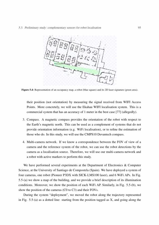
5.3. Preliminary study: complementary sensors for robot localisation 95
Figure 5.4: Representation of an occupancy map, a robot (blue square) and its 2D laser signature (green area).
their position (not orientation) by measuring the signal received from WIFI AccessPoints. More concretely, we will use the Ekahau WIFI localisation system. This is acommercial system that has an accuracy of 1 meter in the best case [77] (allegedly).
3. Compass. A magnetic compass provides the orientation of the robot with respect tothe Earth’s magnetic north. This can be used as a complement of systems that do notprovide orientation information (e.g. WiFi localisation), or to refine the estimation ofthose who do. In this study, we will use the CMPS10 Devantech compass.
4. Multi-camera network. If we know a correspondence between the FOV of view of acamera and the reference system of the robot, we can use the robot detections by thecamera as a localisation source. Therefore, we will use our multi-camera network anda robot with active markers to perform this study.
We have performed several experiments at the Department of Electronics & ComputerScience, at the University of Santiago de Compostela (Spain). We have deployed a system offour cameras, one robot (Pioneer P3DX with SICK-LMS100 laser), and 6 WiFi APs. In Fig.5.5-(a) we show a map of the building, and we provide a brief description of its illuminationconditions. Moreover, we show the position of each WiFi AP. Similarly, in Fig. 5.5-(b), weshow the position of the cameras (C0 to C3) and their FOVs.
During the system “deployment”, we moved the robot along the trajectory representedin Fig. 5.5-(a) as a dotted line: starting from the position tagged as X, and going along the

96 Chapter 5. Multisensor localisation
(a) (b)
Figure 5.5: Representation of the experimental setup for the preliminary robot localisation study. a) Map of thebuilding with a description of its illumination conditions and the positions of the WiFi APs. b) Map ofthe building with the position of the cameras (C0 to C3) and their FOVs.
dashed arrow. Then, we constructed a map from the laser and odometry information usingSimultaneous Localisation And Mapping techniques (SLAM) [51]. After that, we calibratedthe Ekahau location system with the recorded data.
We configured each information source to send data at different rates.
– Cameras: 1 time per second at most. Each camera sends information to the robot (viathe wireless network) when it detects it.
– AMCL (probabilistic localisation): 1 time per 100 milliseconds.
– Ekahau tags (WIFI location): 1 time per second at most. In practice the robot receivesone location reading each 3 to 5 seconds, due to network delays, communication drops,etc.
– Compass: 1 time per 100 milliseconds.
After the “deployment” phase, we performed several tests. In each test, we injected intoAMCL the initial pose of the robot, to ensure a proper initial localisation. Then, we moved therobot around the environment at an average speed of 0.4m/s, following different trajectoriesalong the same corridors shown in Fig. 5.5-(a) (either in clockwise or counter-clockwisedirections). Meanwhile, we recorded each detection of the robot from the cameras, the Ekahaulocation positions, the compass readings, and the succession of poses estimated by the AMCLalgorithm.

5.3. Preliminary study: complementary sensors for robot localisation 97
5.3.1 Robot localisation tests
Figures 5.6 to 5.10 represent five representative robot localisation tests. In each figure, fromleft to right, we represent: the AMCL positions of the robot, its Ekahau positions, and itspositions when each camera detected it (AMCL and Ekahau positions). For the sake of clarity,we down-sampled the AMCL readings by a factor of 10, so we represent 1 AMCL readingper second. Below, we describe each experiment in detail.
In the experiment in Fig. 5.6, we moved the robot clockwise. It is clear that AMCL,Ekahau, and the cameras localised the robot smoothly. It is also clear that Ekahau providesless data than AMCL, since its data rate is lower. In addition, we observe that the periodicityof Ekahau is unstable: for example, the number of Ekahau location readings is significantlylower in region A than in the rest of the experiment. The explanation is simple: the numberof communication failures increased there, primarily between the robot tag and the Ekahauserver. On the other hand, we observe that Ekahau fails to localise the robot in some regions(e.g. B and C), even if no communication failures were observed. This underlines anotherEkahau weakness: its uncertainty, which can go up to 5 meters.
In the experiment in Fig. 5.7, we also moved the robot clockwise. In this experiment,AMCL performed well during the whole experiment. On the other hand, Ekahau failed tolocalise the robot in region A: this was due to communication failures. Particularly remarkableis the fact that cameras C3 and C2 failed to detect the robot (regions B and C respectively).At that time, bright sunlight was coming from the windows (see Fig. 5.5-(a)), which reducedthe apparent intensity of the LED marker as seen from the cameras. As a result, the camerasC2 and C3 were unable to detect the robot. This highlights the importance of working withcomplementary information sources: in this case, if we only relied in the cameras, the robotwould be lost.
In the experiment in Fig. 5.8, the robot movement was counter-clockwise. In this exper-iment, Ekahau performed poorly: it provided very few location readings in regions A and B,and almost no readings in regions C and D. Looking at the high number of robot detectionsfrom the cameras, it is clear that they were able to communicate at all times. On the otherhand, we checked that the robot was able to communicate with the Ekahau server as well.Thus, the Ekahau tag alone failed again to communicate its position to the server, or Ekahaufailed to provide any estimation. Again, this shows that a single information source alone isnot enough to deal with all the possible situations.

98 Chapter 5. Multisensor localisation
In the experiment in Fig. 5.9, the robot movement was counter-clockwise again. Wewould like to emphasise two facts. First, the fact that AMCL got temporarily lost in regionA. This was caused by a small error in the initialisation of AMCL: the initial pose was 0.5meters away from the robot real position. This shows that AMCL performance depends verystrongly on the precision of its initialisation, but it also shows that AMCL is able to recoverfrom this error. Finally, in Fig. 5.9-(d) we can see the big delays suffered by Ekahau. Forexample, when the camera C0 detects the robot in region C, Ekahau considers that the robotis still at region B: in this case, the robot tag informed the Ekahau server about its positionwith a delay of 8 to 10 seconds.
The last experiment is represented in Fig. 5.10. Here, we moved the robot clockwise,but we initialised ACML as if the robot were going to be moved counter-clockwise: in otherwords, the initial AMCL orientation had an error of 180 degrees. As we can see, AMCLlocalisation was incorrect during the whole test: while the real robot path starts and ends atregion A, AMCL estimated that the path started out of the corridors (region B), and ended atregion C, 20 meters away from the real end point. On the contrary, Ekahau and the camerasperformed reasonably well: both could have helped AMCL to recover from the initial error.
Figure 5.6: Test number 1 in the preliminary study for robot localisation.
Figure 5.7: Test number 2 in the preliminary study for robot localisation.

5.3. Preliminary study: complementary sensors for robot localisation 99
Figure 5.8: Test number 3 in the preliminary study for robot localisation.
Figure 5.9: Test number 4 in the preliminary study for robot localisation.
Figure 5.10: Test number 5 in the preliminary study for robot localisation.

100 Chapter 5. Multisensor localisation
Correspondence between map and camera-robot detections
From the Figs. 5.6-(c,d)-5.10-(c,d), we can deduce that it is possible to find a correspondencebetween the FOV of each camera and the area of the map that it covers. This could be doneby matching the camera detections with the AMCL and Ekahau localisation information. Onthe other hand, the position of each camera can be retrieved by placing an Ekahau locationtag in each camera box. We have explored this last option: in Fig. 5.11, we show the suc-cessive camera positions provided by Ekahau during one experiment. Instead of obtaininga single position, we obtain a cloud of positions, due to the inherent uncertainty of Ekahau.Besides robot localisation, this information can be used to establish robust neighbourhoodrelationships among the cameras.
Figure 5.11: Successive positions received from the Ekahau tags attached to the cameras.
Compass
We have also recorded the robot orientation readings provided by the magnetic compass. Werepresent them in Fig. 5.12, as well as the robot orientation provided by the AMCL algorithm.Figure 5.12-(a) represents a counter-clockwise trajectory (initial orientation is 0), and Fig.5.12-(b) represents a clockwise trajectory (initial orientation is 180).
The robot trajectory was square-like, as in Fig 5.5-(a). Thus, at each corner, the robotshould turn 90, and in the end, the robot should have turned 360 in total. For this reason, inFig. 5.12-(a) we represented five regions of interest, A, B, C, D, and E, where the average ori-entation of the robot should be around 0, 90, 180, 270, and 360, respectively. Similarly,

5.3. Preliminary study: complementary sensors for robot localisation 101
Figure 5.12: Robot orientation provided by AMCL and the magnetic compass in two different tests. The orientationrange is [0,360). Therefore, when the orientation is 359 and the robot turns left, the orientationvalue becomes 0. Similarly, when the orientation is 0 and the robot turns right, the orientation valuebecomes 360. a) The navigation direction was counter-clockwise. b) The navigation direction wasclockwise.
in Fig. 5.12-(b), the average orientation of the robot should be around 180, 270, 360, 90,and 180 for regions A, B, C, D, and E, respectively. In absence of a more reliable groundtruth, this can give an insight about the accuracy of the orientation estimations. Note thatthe robot movement was squiggly (Figs. 5.6 to 5.10), what explains the oscillations on theorientation measurements.
From Fig. 5.12, we draw three conclusions. First, the compass is affected by a constantbias, which causes an accumulative error. This bias is typically caused by the presence of fer-

102 Chapter 5. Multisensor localisation
rous objects near the compass: in our case, the metal structure of the robot. A simple compasscalibration should mitigate this effect significantly. Second, even with this bias effect, thecompass error is reasonably low in most cases. This would provide a sufficient accuracy tocomplement the Ekahau location system, and even to improve AMCL estimations when theyare especially erroneous (like in Fig. 5.10-(a)). Third, except for the bias effect, the shape de-scribed by both orientation measurements (AMCL and compass) looks alike, which indicatesthat other ferrous/magnetic elements, such as motors, electric machines, or electric cables,did not affect significantly the performance of the compass. Nevertheless, we are not veryconfident on this, since in other tests we have observed that objects such as vending machinesor data centre rooms cause magnetic interferences that induce important errors.
5.3.2 Conclussions of the preliminary study of robot localisation
From this study, we can draw several conclusions. First of all, we have observed that Ekahauaccuracy is not very high, its measurements arrive with big delay, and any communicationissue affects it strongly. In fact, we have observed that the precision and robustness of Ekahauis very unsatisfactory, despite of being regarded as one of the most precise nowadays [77, 76].Moreover, the Ekahau calibration was tedious, time consuming and error prone, because itrequired us to move all around the environment constantly informing the Ekahau computer ofits position. For these reasons, we have decided to develop our own WiFi localisation system.
More importantly, we have observed that no information source is reliable in all the situa-tions. For example, the cameras can not be used in the presence of direct sunlight, and AMCLperformance depends heavily on the quality of its initial pose estimate. With respect to themagnetic compass, we have seen how ferrous objects near it may cause measurement drifts.On the other hand, Ekahau has several drawbacks as well, as we have already explained. Table5.1 summarises how different situations may affect the performance of each sensor.
On the other hand, we have seen the nature of the errors that affect each information sourcediffers from the rest. Moreover, as we summarise in Table 5.2, each sensor has different prop-erties that make it suitable for situations, but not for others. For instance, WiFi and cameraswork at low data rates and do not give precise estimates of the robot position. This makes themunable to respond rapidly to changes on the robot pose or the environment, therefore they arenot advisable for local localisation (tracking). However, they demonstrated to be very reliablein telling roughly the area were the robot is. Therefore, they can be used for global localisa-tion. On the other hand, laser and compass work at higher data rates and provide very accurate

5.4. Multisensor localisation algorithm 103
Camera WiFi Laser-Map CompassOclussion No Yes No YesOut-of-FOV No Yes Yes YesIllumination No Yes Yes YesCommunication No No Yes YesEM interferences Yes No Yes No
Table 5.1: Is each sensor robust to situations such as occlussion, robot out-of-FOV, severe illumination conditions,communication failures and electro magnetic interferences?
Camera WiFi Laser-Map CompassData rate ≤ 1Hz ≤ 1Hz ≥ 1Hz ≥ 1HzRough global localisation Yes Yes1 No Yes2
Precise local localisation No No Yes Yes2
Table 5.2: Summary of relevant properties of each sensor for mobile robot localisation. 1 Position only, 2
orientation only.
measurements, so they can respond rapidly and accurately to changes on the robot pose or theenvironment. Therefore, they can be used for local localisation (tracking). However, lasercan not distinguish areas with similar geometric structure (e.g. corridors), no matter how farthey are. On the other hand, the compass does not provide position estimates, although theinformation it provides can be relevant both to improve the accuracy of the local localisationestimates, and to reduce the uncertainty when the robot is operating in global localisation.
From this considerations, it seems that each source can complement each other to achievea more robust and redundant system. In the next section, we will propose and validate alocalisation methodology based on the probabilistic fusion of several independent sensors.
5.4 Multisensor localisation algorithm
In the previous section, we have performed an experimental study whose main conclusionwas that the use of complementary sensors could improve the robustness and precision oflocalisation systems. In this section, we will describe and validate an algorithm that is ableto combine the information of several information sources to solve the task of mobile robotlocalisation. Our localisation algorithm is aimed to be used in environments such as museumsor office environments, where layout changes are not frequent. As we have already explained,

104 Chapter 5. Multisensor localisation
we decided that the most functional approach was to build a map of the environment in adeployment stage, and then use this map during the operation stage. Our objective is not topropose yet another localisation algorithm, but to build a localisation system that is robust inreal situations (e.g. people moving around the robot) by fusing the information of multiplesensors.
Most of the main works in mobile robot localisation use Bayesian filtering techniques[51]. These techniques maintain a probabilistic model of the state of a system which evolvesover time and is periodically observed by a sensor (or sensors). From all the Bayesian filter-ing approaches, Kalman filters and particle filters are by far the most popular. Kalman filterswork well when [63] : a) the robot motion is linear, b) the motion and sensor noises are white,Gaussian and can be modelled accurately, c) there is an explicit and unimodal mapping (obser-vation model) between states and observations, and d) the best estimate of the state is unique(unimodal probability distribution over the state space). Some of these conditions do not holdin the context of robot localisation. For instance, the robot movement is usually non-linear,although this would not be a critical issue, given the low linear and turn acceleration that ourrobots can achieve. Moreover, Kalman filter variants such as the Extended Kalman Filter orthe Unscented Kalman Filter [51] could be used. However, other restrictions are critical in ourcontext. For instance, in practice it may be hard to model with Gaussian distributions the ob-servation models and their noises. Above all, the most important problem is that observationmodels and therefore state probability distributions are usually multi-modal.
Particle filters [51] are a powerful yet efficient alternative to Kalman filters. Particle fil-ters do not make any of the previous assumptions. First of all, they work with non-linearnon-Gaussian systems with multi-modal probability distributions, where there is no explicitmapping between sensor observations and system states. This allows us to maintain sev-eral localisation estimates simultaneously, which is very useful when sensor readings are notsufficiently discriminative to estimate an unique position. Moreover, with particle filters theprobabilistic mapping between sensor measurements and position candidates can follow anyprobabilistic distribution. This provides us with a great flexibility when modelling the locali-sation sensors. Moreover, these filters are very robust even if the system and sensor noises arepoorly estimated [63]. Therefore, particle filters will be our choice in order to implement ourlocalisation algorithm.
Our localisation system has to estimate, at every instant t, the pose of the robot (state) st =
(xt ,yt ,θt) with respect to a map, where (xt ,yt) represents the position in cartesian coordinates,

5.4. Multisensor localisation algorithm 105
and θt the orientation. Our system estimates this pose based on: 1) perceptual informationZt = z1
t , ...,znz
tt (set of nz
t sensor measurements available at time t), and 2) control data ut
(the robot movement as provided by odometry encoders). In addition, we will estimate Σt(s)
(the covariance of st ). In order to accomplish our goal, our system iterates over a two-stepprocess:
1. Pose probability estimation (Secs. 5.4.1-5.4.2). This step computes the pose probabilitydistribution over all possible robot poses. This distribution is usually called the belief
distribution, and it represents the belief that any possible pose refers to the actual currentposition and orientation of the robot. As the pose of the robot changes over time so doesthe belief distribution bel(st).
2. Pose estimation (Sec. 5.4.2). Estimation of the most likely current pose st from thepose probability distribution bel(st).
5.4.1 Recursive Bayes filtering to estimate the pose probability distri-bution
In the Bayesian filtering approach to dynamic pose estimation, the belief distribution is theposterior probability density function of the pose based on all the available information, i.e.the set of actions taken by the robot ut:1 = ut ,ut−1, ...,u1, and the set of received sensormeasurements Zt:1 = Zt ,Zt−1, ...,Z1 [63, 99].
bel(st) = p(st |Zt:1,ut:1) (5.1)
In our case, an estimate of the robot’s pose is required every time that the robot performsan action and receives a set of sensor measurements. Computation of Eq. 5.1 requires to storethe complete data set, and process it as a batch when new data becomes available. Instead,a recursive filter is a much more convenient solution: the received data can be processedsequentially, and previous data can be discarded. One can derive such filter by using theBayes rule [63]:
bel(st) ∝ p(Zt |st ,Zt−1:1,ut:1)p(st |Zt−1:1,ut:1) (5.2)
and the law of total probability [63]:
bel(st) ∝ p(Zt |st ,Zt−1:1,ut:1)∫
p(st |st−1,Zt−1:1,ut:1)bel(st−1)dst−1 (5.3)

106 Chapter 5. Multisensor localisation
The recursive Bayes filter in the context of robot localisation is also known as Markovlocalisation, because of what is called the Markov assumption [63]. This assumption statesthat past and future data are independent if one knows the current state (pose). In other words,provided the current state, past states or data are not relevant to future predictions. Therefore,the knowledge of st−1 and ut is enough to predict st :
p(st |st−1,Zt−1:1,ut:1) = p(st |st−1,ut) (5.4)
Similarly, the knowledge of st is enough to predict Zt :
p(Zt |st ,Zt−1:1,ut:1) = p(Zt |st) (5.5)
Therefore Eq. 5.3 can be rewritten as:
bel(st) ∝ p(Zt |st)∫
p(st |st−1,ut)bel(st−1)dst−1 (5.6)
This is the general form of the recursive Bayes filter, represented in Fig. 5.13. Initially,the first belief distribution bel0(s) may be initialised randomly, e.g. following an uniformdistribution. Then, the filter performs iteratively in two stages: prediction and update.
Figure 5.13: Block diagram of the recursive Bayes filter for mobile robot localisation.

5.4. Multisensor localisation algorithm 107
Prediction
The prediction stage predicts a new belief distribution ˆbel(st) of the pose of the robot from oneinstant to the next one, considering the current actions taken by the robot ut (robot movement)and the previous distribution bel(st−1).
ˆbel(st) =∫
p(st |st−1,ut) bel(st−1) dst−1 (5.7)
The term p(st |st−1,ut) is called the motion model of the robot. It describes, from a prob-abilistic perspective, the evolution of the pose when only the actions taken by the robot areconsidered. This model depends on the specific kinematics of the robot (i.e. how much itsposition will evolve considering the angular and linear velocities performed).
Update
The update stage uses the latest sensor measurements Zt to correct the belief distributionpreviously predicted ˆbel(st), producing the true posterior distribution bel(st):
bel(st) ∝ p(Zt |st) · ˆbel(st) (5.8)
The function p(Zt |st) is called the observation model: it specifies the probability of re-ceiving a certain measurement Zt provided that the robot is in a certain pose st . Therefore,Eq. 5.8 corrects ˆbel(st) based on the similarity between the sensor data received Zt and thesensor data expected to be received from each possible pose st . Under this approach, the mostprobable poses will be those with the highest similarity between expected and received sensordata.
The joint probability function p(Zt |st) is hard to estimate in practice, specially if we havenon-synchronised sensors that work at different rates. Assuming that the sensors are condi-tionally independent provided st :
bel(st) ∝ ˆbel(st)nz
t
∏k=1
p(zkt |st) (5.9)
Note that each observation model depends on the specific sensor that it represents (we willexplain in Sec. 5.5 how these models are obtained). Moreover, note that at each instant t weonly take into account Zt , the set of nt
z readings received at that instant. In other words, thealgorithm does not require a reading from every sensor at each update. Therefore, the sensors

108 Chapter 5. Multisensor localisation
do not need to be synchronised, because the algorithm will integrate their information when itis available. For the same reason, the sensors do not need to have the same data rate. However,in practice it is a good idea to not allow a sensor to provide data much faster than the rest (e.g.10 times faster), because it would dominate the fusion. Finally, since Eq. 5.9 allows us tohave a variable number of sensors, the algorithm will continue working even if some sensorsstop providing data. Moreover, we can include new sensors in the fusion process even if therobot is in operation. All these situations are very challenging but our system handles themproperly, as we will see in Sec. 5.7. This ensures the robustness and scalability of the fusionmethodology.
5.4.2 Implementation of the recursive Bayes filtering with particle fil-ters
The problem of the Bayesian filtering described before is that in practice it is not straight-forward to compute belt(s). However, there exist several methods to approximate probabilitydensity functions (PDFs) as mixture models, that is, as the weighted sum of a finite numberof simple distributions, usually known as kernels. One popular method is the Sequential Im-portance Sampling (SIS) algorithm (also known as particle filter) [63, 99, 100, 101], whichimplements the recursive Bayesian filter described above using sequential Monte Carlo simu-lations.
This method is based on the following idea. Assume that, at time t, we have a set ofnp samples from bel(st) (usually called particles). This sample set will be represented asPt = Pi
t = (sit ,ω
it ), ∀ i ∈ 1, ...,np , where si
t is the pose of the sample, and ω it a weight
associated to the sample (the sum of the weights must add up to 1). In this case, we couldapproximate bel(st) as [100, 101]:
bel(st)≈np
∑i=1
ωit ·δ (si
t − st) (5.10)
where δ (sit − st) is the Dirac’s delta function centred at si
t . Note that the more weightthe particle has, the more likely its pose is. Unfortunately, we can not easily take samplesfrom the marginal distribution bel(st) = p(st |Zt:1,ut:1) [100]. Instead, we will sample fromp(st:0|Zt:1,ut:1) (target distribution), and ignore the samples st−1:0. The samples are cho-sen using the principle of importance sampling [100, 101]: since the target distribution isunknown, we will sample from a proposal distribution q(st:0|Zt:1,ut:1) defined by us (from

5.4. Multisensor localisation algorithm 109
which it is easy to take samples) and weight each sample i according to:
ωit =
p(sit:0|Zt:1,ut:1)
q(sit:0|Zt:1,ut:1)
(5.11)
Assuming that the following factorisation is possible (Markov assumption):
q(st:0|Zt:1,ut:1) = q(st |st−1,Zt ,ut)q(st−1:0|Zt−1:1,ut−1:1) (5.12)
it can be shown that we can compute Eq. 5.11 recursively in terms of ω it−1 [100, 101]:
ωit ∝
p(Zt |sit)p(si
t |sit−1,ut)
q(sit |si
t−1,Zt ,ut)ω
it−1 (5.13)
Therefore, at time t we can simply sample a new pose for each particle from the proposaldistribution q(st |st−1,Zt ,ut). A convenient choice for this function is the motion model of therobot:
q(st |st−1,Zt ,ut) = p(st |st−1,ut) (5.14)
Consequently:ω
it ∝ ω
it−1 p(Zt |si
t) (5.15)
With this in mind, our particle filter performs as follows. First of all, a set of particles P0
is generated with random poses si0 and equal weights ω i
0. Then, the algorithm iterates over thefollowing steps:
1. Prediction. With each robot displacement ut , we sample a new pose sit for each particle
using the robot motion model:
sit ∼ p(st |si
t−1,ut) ∀ i ∈ 1, ...,np (5.16)
In practice, this can be interpreted as a displacement of each particle as indicated byut , plus some random noise in position and orientation to accommodate the error of theodometry of the robot (see [63] for details and other options).
2. Update. We correct the weight of each particle with Zt (sensor information available attime t):
ωit ∝ ω
it−1 p(Zt |si
t) = ωit−1
nzt
∏k=1
p(zkt |si
t) (5.17)
This way, each particle will integrate the past sensor information (using the previousweight) and the fusion of the current sensor information. The weights are normalisedto sum up to one.

110 Chapter 5. Multisensor localisation
Resampling
The particle filter algorithm suffers from the sample depletion phenomenon [101, 102]: aftera while, all but one particle will have negligible weights. The degree of depletion can bedefined as the effective number of effective particles [101, 102]:
Ne f f =1
∑npi=1(ω
it )
2(5.18)
The maximum number of effective particles is Ne f f = np, when all weights are equal(ω i
t = 1/np, lower degree of depletion). The minimum number of particles is Ne f f = 1, whenonly one particle accumulates all the weight (this is undesirable, highest degree of depletion).
In order to correct the depletion phenomenon, it is common to perform a resampling stepwhen the number of effective particles falls below a certain threshold value (e.g. 2
3 np). The re-sampling step consists on the construction of a new set of particles from the current one. Firstof all, we take nnr particles from the current set with probability proportional to their weightusing the Low Variance Resampling technique [63] (we may repeat particles). Secondly, wegenerate a variable number nr of random particles (nnr +nr = np). The generation of randomparticles allows the algorithm to recover when it converges erroneously to a wrong pose. Wecalculate nr by keeping a long term average ω l
t and a short term average ωst of the weight of
the particle set:
ωlt = ω
lt−1 +α
l ·
(1np
np
∑i=1
ωit −ω
lt−1
)(5.19)
ωst = ω
st−1 +α
s ·
(1np
np
∑i=1
ωit −ω
st−1
)(5.20)
nr =
⌈np ·max
(0,1− ωs
t
ω lt
)⌉(5.21)
where 0 < α l << αs < 1. The ratio ωst /ω l
t estimates whether the quality of the particle setis increasing (increasing ratio) or decreasing (decreasing ratio). Therefore, the more this ratiodecreases, the more random particles we generate.
The impact of the resampling step can be seen in Fig. 5.14. In Fig. 5.14-(a), the particleswere initialised randomly. Then, the robot started to move and to integrate information, goingthrough cycles of prediction and update steps. This lead to particles with different weights,and therefore to several resampling steps. Figs. 5.14-(b-c) show the evolution of the cloud ofparticles after the occurrence of succesive resamplings. Observe that the algorithm tends to

5.4. Multisensor localisation algorithm 111
(a) (b)
(c) (d)
Figure 5.14: Particle filter evolution. a) Initially, all the particles are distributed randomly across the environment.b-c) Soon, particles start to concentrate around the most problable areas (given a number of sensorreadings and robot displacements). d) Finally, most particles converge around the most probable pose(bottom-right part of the image).
accumulate particles in the areas where the robot might be with the highest probability, untilit converges to the true robot pose (Fig. 5.14-(d)).
Pose estimation
At this point, we have computed bel(st), and we need to estimate the most likely pose st :
st = argmaxsbel(st) (5.22)

112 Chapter 5. Multisensor localisation
In our case, we have to estimate this pose from the particle set Pt . There are many othermethods to achieve this: a weighted mean over all the particles is one of the most popular [63].However, in some cases methods based on simple analytics like that one might deal strangeresults. For instance, when we have two or more bulks of particles with similar weights indifferent positions, a weighted mean would estimate that the correct position is between thesetwo sets, in the region of lowest probability.
To solve these issues, we propose a clustering based process. The key idea is that mostparticles will concentrate in few regions (the most likely regions), therefore we should be ableto detect pose hypotheses (clusters of particles), and select one of them. To this extent, weperform the following two-step process:
1. Hypothesis generation. First of all, we use agglomerate clustering [103] to group theparticles in clusters. Each particle will be assigned to its closest cluster, provided thatthe distance between the particle and the cluster centroid is lower than a threshold dis-tance in position distth−xy and in orientation distth−θ . Otherwise, the particle will createa new cluster. Each cluster i can be interpreted as an hypothesis about the position ofthe robot. We will represent each hypothesis as H i
t = Ωit ,µ
it ,Σ
it, where Ωi
t is the totalweight of the particles contained in the cluster i, µ i
t is the average pose of the particlesof the cluster, and Σi
t is their covariance matrix. The influence of each particle on thesetwo statistics (mean and covariance) is proportional to its weight.
2. Hypothesis selection. We will select the hypothesis that accumulates more weight, pro-vided that this accumulated weight exceeds certain threshold: Ωi
t > Ωth (Ωth ∈ [0.5,1]).Then, the robot pose st will be µ i
t and the covariance Σt(s) will be Σit . In the next step,
this hypothesis will be chosen again if Ωit > 1−Ωth. This increases the stability of the
hypothesis selection.
5.5 Sensor observation models
Our system fuses the information from all the sensors using their observation models (Eq.5.17). In order to train the observation models, we must: 1) capture a number of measurementsat different points of the environment (calibration data), and 2) build the training sets. Thislast step requires us to relate each measurement with the position where it was measured.There exist a number of alternatives to accomplish this. For instance, there are systems that

5.5. Sensor observation models 113
provide the position of the robot at every instant (e.g. external infrared cameras for 3D markertracking, such as Tracking Tools from Natural Point). However, these systems are extremelyexpensive and adequate only for small areas. As an alternative, an user may indicate whereeach measurement took place, but this method has some serious drawbacks: it is tedious, timeconsuming and error prone. Instead, we follow the procedure depicted in Fig. 5.15 and whichcan be summarised in the following steps:
1. Collect the calibration data by moving the robot around the environment. The condi-tions of the environment must favour the quality of the data (e.g. no people movingaround the robot).
2. Process the collected data off-line.
a) Build the occupancy map of the environment: a grid where each cell may cor-respond with free or occupied space. Figure 5.16 contains an example of an oc-
Figure 5.15: Procedure to calibrate the observation models.

114 Chapter 5. Multisensor localisation
cupancy map. To construct this map we use an SLAM algorithm with laser andodometry information.
b) Compute the trajectory followed by the robot and associate each pose with itstimestamp (xt ,yt ,θt).
c) Build a training set for each sensor. Each training set contains the data capturedby a sensor associated with the corresponding pose (zi
t ,xt ,yt ,θt ).
d) Train the observation model of each sensor (p(zi,s)).
Our sensor fusion methodology allows us to use a variable number of sensors of differentnature (we discuss some practical constraints in Sec. 5.6.3). To demonstrate the performanceof this methodology in practice, we will use a 2D laser range-finder, an WiFi receiver, a mag-netic compass, an external camera network, and a camera mounted on the robot. Hereafter,we will propose an observation model and a mapping strategy for each sensor. We follow ageneral methodology that allows us to calibrate the sensors with few data (fast deployment)avoiding overfitting, and that can be easily adapted to other sensors.
Figure 5.16: Example of a laser occupancy map MO. White represents free space, black represents occupied space,and grey represents unknown space.

5.5. Sensor observation models 115
5.5.1 2D laser rangefinder - Observation model
At any time instant t, a 2D laser range finder provides a set zlt = l1
t , ..., lnlt of nl range mea-
surements among the robot and the nearby objects. All ranges are on the same plane (typically,parallel to the ground), each one pointing on a different angle. This vector is usually called thelaser signature. The signatures observed at different poses are usually different: therefore, wecan compute the likelihood of a certain pose depending on how much the signature receivedresembles the one expected from that pose.
To this extent, we must build a map of expected signatures. We will refer to this map asthe laser ranges map MLR. The occupancy map MO serves as a base to calculate MLR. Foreach cell, we calculate a vector of distances between the cell and the nearest occupied cell(in several radial directions, with a certain angular resolution). We use MLR to calculate theexpected laser signature zl(s) = l1(s), ..., lnl
(s) at each possible robot pose according to themap. With this information, we approximate the laser observation model by the similaritybetween zl(s) and zl
t :p(zl
t |s) = hd(zl(s),zlt) · td(zl(s),zl
t) (5.23)
where hd(zl(s),zlt) estimates the shape similarity among both laser scans (measured and
expected) using the Hellinger distance [104]:
hd(zl(s),zlt) =
1−
nl
∑i=1
√li(s) · li
t
1nl
√nl
∑i=1
li(s)nl
∑i=1
lit
1/2
(5.24)
and td(zl(s),zlt) takes scale into account by calculating the average difference among each
pair of range measurements (li(s), lit ), normalized in the range [0,1] using a triangular func-
tion:
td(zl(s),zlt) =
[1nl
nl
∑i=1
max(
1− |li(s)− li
t |maxLD
,0)]
(5.25)
The parameter maxLD (maximum laser difference) indicates the maximum allowed differ-ence among each pair of laser ranges.
5.5.2 WiFi - Observation model
There are several technologies that have been used in wireless indoor positioning [75, 76, 77],such as RFID, UWB, Bluetooth, TV, or GSM. However, WiFi positioning has been the most

116 Chapter 5. Multisensor localisation
popular alternative by far. WiFi localisation is usually based on fingerprinting [105, 106]. Fin-gerprinting refers to techniques that: 1) on a calibration stage, collect features or fingerprints
of the wireless signal and the location where they were measured to build a radio map, and 2)on a use stage, estimate the position of the receptor by matching online measurements withthe radio map. Usually, the RSSI (Received Signal Strength Indication) features are used,which are related to the signal power received from the Access Points.
There are two basic kinds of radio-maps that can be constructed with fingerprinting tech-niques: model-based and empirical maps [105]. Model-based maps are defined by a set ofparameters that specify the characteristics of the environment (e.g. walls, materials, etc.)and/or the characteristics of the signal propagation. These parameters are usually adjustedusing calibration data. On the other hand, empirical methods (which tend to achieve better re-sults [107, 108]), work directly with the fingerprints to build radio maps. There are two kindsof empirical maps: deterministic and probabilistic maps [105]. Deterministic maps assign asingle value to each position of the map, such as a fingerprint in that position, or an average ofthe closest fingerprints. The most important drawback of these maps is that a single value cannot capture the random nature of wireless signals. As a solution, probabilistic maps charac-terise the wireless signal at each position using probability distributions [106] (e.g. Gaussian,Log-Normal, Weibull, etc.).
On the other hand, almost any algorithm from the fields of machine learning and estima-tion could be used as a position estimation method. Usually, estimation methods are dividedin two groups [105, 106]: deterministic and probabilistic. Deterministic methods estimate thelocation of the receptor directly from the value of the measurements received. Techniquessuch as Artificial Neural Networks [109, 110], Support Vector Machines [73, 111] and Near-est Neighbours and its variants [106, 112, 107] have been used to implement deterministiclocalisation techniques. On the other hand, probabilistic methods estimate the position ofthe device as part of a random process. Usually, they integrate the measurements sequen-tially, and exploit information about the movement of the device or about the topology ofthe environment. It has been shown that probabilistic techniques tend to have better resultsthan deterministic ones [106]. Probabilistic methods are usually based on Bayesian inference[106], Hidden Markov Models [113], or particle filters [73, 114].
In this section, we will explore the use of empirical probabilistic maps and probabilisticalgorithms for wireless positioning. We will capture the data that we will use to build the radiomap with a WiFi card on-board the robot. This card is able to receive the signal power from

5.5. Sensor observation models 117
the WiFi APs in the environment. This information can be represented as zwt = w1
t , ...,wnw
tt ,
where nwt is the number of APs available at time t, and wi
t is the power in dBms of the ith APat time t. Using the data captured at the “data collection” stage (Fig. 5.15), we build a trainingset for each AP Dw
i = (xt ,yt) ; wit). Each sample of the training set consists on an output
wit (power of the ith AP received from the scan at time t), associated with an input (xt ,yt)
(position where the scan took place).This “fingerprinting” data set can be used to calibrate the WiFi observation models using
several supervised learning techniques. Essentially, we want to know the probability of re-ceiving a certain measurement zw
t when the robot is in any position (xt ,yt). In this thesis, wewill explore different options in order to achieve this goal. In short, these options are:
1. Compute the most probable position (xwt , y
wt ) for a certain measurement. This can be
achieved with any regression technique, trained with the measurements as inputs andthe positions where they were taken as outputs. Then, we can define the observationmodel as a function of probability around that position. In our case, we have tested theperformance of the ε-Support Vector Regression technique.
2. Compute directly the probability of receiving a certain measurement zwt from every
position (xt ,yt). This can be achieved in two different ways:
a) Estimating from training data the expected measurement values zwt at each posi-
tion (xt ,yt). This can be easily achieved with spatial regression techniques, trainedwith the positions were we have taken measurement as inputs, and the actual mea-surements as outputs. Then, we can compute the differences between zw
t and zwt at
each position, to define the observation model as a function of these differences.In this thesis, we have used the Gaussian Processes Regression technique (GPregression).
b) Estimating, for each measurement in the training set, the density function of itsoccurrences in the whole space. This can be achieved with any density func-tion estimation technique. The training input is a collection of measurementsand the positions where they were taken, and the output the estimated densityacross space. Therefore, the observation model will be defined by these densityfunctions: when a new measurement arrives, its probability will be related to thedensity of occurrence of that measurement at each position. In our case, we haveused a technique based on Gaussian Mixture Models.

118 Chapter 5. Multisensor localisation
Computation of the most probable position: ε-Support Vector Regression
The first strategy we have tested to create the WiFi observation model consists on translatingthe Wi-Fi measurements zw
t into an intermediate estimate of the robot’s position (xwt , y
wt ), and
then obtain the measurement model from these estimations. In order to estimate xwt and yw
t ,we use two regression functions f w
x and f wy :
xwt = f w
x (w1t , ...,w
nw
t ) (5.26)
ywt = f w
y (w1t , ...,w
nw
t ) (5.27)
where nw is the number of APs in the environment, and wit is the power in dBms of the ith
AP at time t. In order to learn f wx and f w
y , we have chosen the ε-Support Vector Regressiontechnique with Gaussian Radial Basis Function kernels (ε-SVR-RBF) [115]. The predictionerror of the ε-SVR-RBF can be approximated by a zero mean Laplace distribution [115], andtherefore the observation model of our Wi-Fi sensor is defined by Eq. 5.28:
p(zwt |s) =
[1
2σw(x)exp(−|x
w− x|σw(x)
)][1
2σw(y)exp(−|y
w− y|σw(y)
)](5.28)
where σw(x) and σw(y) are the noise parameters, which can be estimated from training data.
Computation of expected values at each position: Gaussian Processes Re-gression
The second strategy that we have analysed to create the WiFi observation model consists onestimating the expected measurement values zw
t at each position (xt ,yt), and then deriving theobservation model. We have mentioned that we could use any spatial regression techniquefor this purpose. In this thesis, we will used Gaussian Processes regression (GP regression)[116].
GP regression has already been described as a powerful tool to solve regression problems,and has already been used with great success to build probabilistic radio-maps [80, 117].Particularly, Duvallet et al. described several of their advantages to map the WiFi signal[80]. These advantages apply to the compass and the cameras as well. First, GPs are non-parametric, so they do not require a regression model to fit the data. Second, both linear andnon-linear models may emerge from the regression (whichever fits best the data). Third, GPsare continuous, meaning that: a) training points do not have to be gathered at regularly spaced

5.5. Sensor observation models 119
intervals, b) the environment does not need to be discretised, and c) predictions can be gen-erated for any point in the environment. Finally, contrary to other alternatives such as ε-SVR[57], GPs correctly handle uncertainty in both the process and the estimation and naturallyprovide probabilistic estimations. We would like to add to this list that GPs are speciallysuited to solve 2D spatial regression problems, because of the use of a kernel function thatcan model the spatial correlation among nearby points in the environment. In addition, due totheir probabilistic nature, GP regression techniques provide probabilistic observation models,therefore they can be integrated naturally with Bayesian inference algorithms [80, 117].
As in any regression problem, GP regression attempts at predicting a continuous output ofa system for any arbitrary input d∗in. Gaussian Processes are a supervised learning technique,therefore they require a training data set D = (din;dout)|i = 1, ...,n. This data set consistson n samples in Rd such that:
dout = f (din)+ ε (5.29)
where f is the function that defines the system, and ε is additive Gaussian noise with zeromean and variance σ2
n . Following a matrix notation, Din is the d×n matrix containing the setof training inputs, and dout the 1×n vector containing the set of training outputs.
GPs rely on a covariance function kernel k(dpin,d
qin) that specifies the correlation among
inputs. The idea behind this function is that input points that are close to each other are likelyto have similar output values. There are many choices for this kernel [116], but in this thesiswe have used the squared exponential kernel [80]:
k(dpin,d
qin) = σ
2f exp
(−1
2(dp
in−dqin)
tL(dpin−dq
in)
)(5.30)
where L is a diagonal matrix whose diagonal elements are scale parameters of the kernelfor each dimension of the input. This kernel can be represented as a matrix K. Moreover, wewill represent as k∗ the vector of covariances between an arbitrary input d∗in and the traininginputs in Din. The covariance among inputs leads to the definition of the covariance amongoutputs:
cov(dpout ,d
qout) = K +σ
2n I, (5.31)
where I is the identity matrix and σ2n is the observation noise.
Gaussian Processes do not compute the function f directly. Instead, they define a distri-bution of probability over functions that aim at explaining the training data. For any arbitraryinput point d∗in, the posterior distribution over these functions will be:

120 Chapter 5. Multisensor localisation
p( f (d∗in)|d∗in,D)∼N (µ∗,σ∗2) (5.32)
whereµ∗ = k∗t(K +σ
2n I)−1dout (5.33)
σ∗2 = k(d∗in,d∗in)− k∗t(K +σ
2n I)−1k∗ (5.34)
In other words, given any input d∗in and a training set D, GP regression predicts a prob-abilistic output defined as a normal function centred in µ∗ (most probable output) with atypical deviation of σ∗. The typical deviation models the noise in the training data and theuncertainty of the prediction at the same time. All the parameters of the GP regression canbe learned from training data by maximizing the log marginal likelihood of the observationsconditioned on the parameters [116].
In our case, the regression will compute, for each AP, the functions µwi (x,y) and σw
i (x,y).These functions represent the average and the typical deviation of the signal strength of theith AP across the environment. Figure 5.17 shows a representation of these functions for asample AP.
These functions will be the base of the observation model of the WiFi. First of all, we willcompute the observation model of each AP independently:
p(wit |s) ∝
1λ wσw
i (x,y)√
2πexp
[−1
2
(wi
t −µwi (x,y)
λ wσwi (x,y)
)2]
(5.35)
(a) µwi (x,y) (b) σw
i (x,y)
Figure 5.17: Output of the Gaussian Process regression for a sample WiFi AP. a) The lowest values (red)correspond to the highest power. It is clear that the AP was located near the position (10m, 10m), andthat the propagation of the WiFi signal is not isotropic, therefore very hard to model analytically. b)The lowest values (red) correspond to the lowest typical deviation power.

5.5. Sensor observation models 121
where λ w is a parameter that scales the typical deviation estimated by the GP regression.Therefore, it modifies the confidence that we have in the sensor model (the greater λ w, thelower the confidence and the higher the tolerance towards noise). If we assume that thetransmitters are conditionally independent given an arbitrary pose s:
p(zwt |s) ∝
nwt
∏i=1
p(wit |s) (5.36)
where p(wit |s) represents the probability that the robot receives a signal power wi
t from theith transmitter, assuming that the robot is at pose s.
In our experience this approximation is not robust, because it depends too much on theoutput of each individual function p(wi
t |s). This is because the combination is a product ofprobabilities, so even if most functions agree on a certain pose, a single function that has avalue near zero around that pose will cause the product to fall close to zero. This is representedin Fig. 5.18-(a), where even if most models p(wi
t |s) would predict a position around s ≈ 0(probably correctly), a single model (p(w5
t |s)) is enough to distort the prediction p(zwt |s) so
that the maximum falls at a intersection between all the distributions (probably incorrect).This represents an issue because even small noises on the power received from the transmitterscan have a big impact on the robustness of the predictions.
We would like to remark that wireless signal power measurements fluctuate due to severalfactors, such as hardware construction of the receiver, device orientation, human presence,humidity, and changes in the environment such as open/locked doors (see [81, 82, 83, 84, 85,86]). For instance, in [81] fluctuations of up to ±7.5 dBm were reported in static environ-ments. Similarly, in [82] variations of 3dBm were observed depending on the orientation ofthe wireless receiver, and the presence of people caused differences of up to 8dBm. These ef-fects are much more drastic in environments were multipath signal propagation does not exist[118]. However, this is not the case of indoor wireless positioning, because in indoor spacesthere always exist more than one propagation path from transmitter to receiver. Obviously,these fluctuations have an effect on the positioning error. For instance, in [84] the positioningerror increased from 2.10m in ideal conditions to 3.06m due to changes in humidity, to 3.96m
due to the presence of people, and to 7.17 m due to the effect of opens doors.Therefore, a simple voting scheme can be a much more robust solution:
p(zwt |s) ∝
nwt
∑i=1
p(wit |s) (5.37)

122 Chapter 5. Multisensor localisation
(a) (b)
Figure 5.18: Likelihood distribution resultant from: a) Eq. 5.36 (product), b) Eq. 5.37 (sum). Each blue linerepresents an individual function p(wi
t |s), and the green line the fusion of these functions using Eq.5.36 or 5.37, respectively.
The underlying idea is that each individual model can contribute to the final prediction,but no model should have such an influence as in Eq. 5.36. Essentially, Eq. 5.37 solvesthis problem by aggregating the individual probabilities. This is represented in Fig. 5.18-(b),where the maximum value of p(zw
t |s) is achieved where most p(wit |s) achieve their respective
maximum (where most distributions agree), which is probably the correct prediction. Theresultant distribution is therefore less affected by individual fluctuations.
Figure 5.19 shows two examples of this likelihood distribution when the robot is at twodifferent positions. Note that in both cases the distribution is multi-modal, but there is usuallyan area that concentrates most of the likelihood.
(a) (b)
Figure 5.19: Likelihood distribution provided by the WiFi observation model for two different sensor readings(highest values in blue, lowest values in red).

5.5. Sensor observation models 123
Computation of density functions: Gaussian Mixture Models
In the previous section, we have estimated the expected measurement values zwt at each posi-
tion (xt ,yt) from training data using GP Regression. Then, we have shown how to computethe observation model taking into account the difference between the received measurementszw
t and the expected measurements zwt at each position. In this section, we will estimate di-
rectly the probability of receiving a measurement based on the density of occurrence of thatmeasurement at each position. This can be achieved using density estimation techniques, suchas Gaussian Mixture Models [119].
A density estimation problem can be defined as follows: given a set D = d1, ...,dN of N
data points in nd dimensions, and a family F of probability density functions on Rnd , find theprobability density f (d) that is most likely to have generated those points. Mixture Modelstry to compute this function f (d) as a weighted sum of K functions fk(d):
f (d) =K
∑k=1
λk fk(d) (5.38)
where the numbers λk are called the mixture probabilities, because λk≥ 0 and ∑Kk=1 λk = 1.
In principle, the family F could be formed by completely arbitrary functions, but in practice itis common to use parametric mixture models, where the functions fk(d) are all from the sameparametric family, so the model becomes:
f (d) =K
∑k=1
λk fk(d;θk) (5.39)
where θk are the parameters of each function fk(d). A usual choice is to use a family F ofGaussian functions, therefore:
f (d) =K
∑k=1
λkN (d; µk,Σk) (5.40)
The mixture model has a set of parameters θ = λ1, . . . ,λk,µ1, . . . ,µk,Σ1, . . . ,Σk. Thedensity estimation problem can now be defined as the problem of finding the vector θ ofparameters that specifies the model from which the training points are most likely to be drawn.To this extent, we will use the Maximum Likelihood criteria, which defines the likelihood ofobserving the data as a function of the parameters. Assuming independent data:
l(θ) =N
∏n=1
f (dn;θ) (5.41)

124 Chapter 5. Multisensor localisation
For Mixtures of Gaussians, we have:
l(θ) =N
∏n=1
K
∑k=1
λkN (d; µk,Σk) (5.42)
and the parametric density estimation problem will be solved by finding the vector θ thatmaximises this likelihood function, that is:
θ = argmaxθ
l(θ) (5.43)
To achieve this, we can use any maximisation algorithm. Particularly, we have used theExpectation-Maximisation algorithm [119], which works particularly well for this problem.More precisely, we have computed a density function for each WiFi AP, using the trainingsets Dw
i that we have captured during the deployment stage. In this case, the training inputswill be of the form (xt ,yt ,wi
t), and the output will be directly the density of occurrence of eachdata point. Therefore, the observation model of each AP can be defined as:
p(wit |s) =
K
∑k=1
λkN (d; µk,Σk) (5.44)
and the complete observation model can be computed by combining the observation mod-els of all the APs using a simple voting scheme:
p(zwt |s) ∝
nwt
∑i=1
p(wit |s) (5.45)
In practice, we did not achieve satisfactory results using this method. We found the fol-lowing issues:
– The algorithm tends to overfit. This is expectable, because in a context of fast de-ployment the ratio between the amount of data and the size of the environment is low,therefore the training data will not be very diverse. However, we have observed that thismethod overfits more than the GP regression approach. We have tried to add syntheticdata to increase the noise of the training set. This improved the results, but they werestill not satisfactory.
– No spatial interpolation capability. The overfit makes Gaussian functions to have smallcovariance components. Therefore, in the areas where we do not have training data themodel always gives us probability values near to zero (e.g. areas farther away than 1metre from the nearest training point).
5.5. Sensor observation models 125
– Penalisation of areas with a low number of training points. The algorithm tries to ex-plain the data “in average”. In practice, this means that the Gaussians will tend to becentred around areas near the centre of the map (where we usually have more trainingpoints), but not on the periphery. Therefore, the results on the periphery are usually notgood. We could solve this by balancing the data, but since we already have few datapoints, this does not give good results.
Given these problems, in this thesis we did not use this method in real robot operation.
5.5.3 Magnetic compass - Observation model
A magnetic compass is a low cost sensor available in many robots. It provides the orientationzc
t = θ ct of the robot with respect to the Earth’s magnetic north. The compass measurements
are affected by magnetic fields produced by elements common in public indoor environments,like metallic structures, vending machines, etc. Therefore, the observation model shouldaccount for the existance of these distortions. We will explore two ways of modelling thesenoises:
1. Assuming that the probability of distortion does not vary across the environment (sta-tionary distortion).
2. Assuming that the probabilty of distortion changes depending on where the robot is(non stationary distortion).
Stationary distortion
In this case, we will assume that the measurement noise is Gaussian and independent of therobot position:
p(zc|s) = 1σ c√
2πexp
[−1
2
(θc−θ
σ c
)2]
(5.46)
where θ is the orientation component of the robot pose s, and σ c is a noise parameter of thissensor, which can be estimated experimentally. This assumption is reasonable in absence ofstrong magnetic interferences, which would require a more complex alternative.

126 Chapter 5. Multisensor localisation
Non-stationary distortion
In this case, we must model the distortion across the whole environment. First of all, wecollect a set of k true robot orientations θ T = θ T
1 , ...,θTk , and we store the corresponding set
of compass readings θ c = θ c1 , ...,θ
ck . Then, we compute the differences among both sets:
ec = ec1, ...,e
ck= |θ c
1 −θT1 |, ..., |θ c
k −θTk | (5.47)
Wherever the spurious magnetic interference is strong, this difference (error) will be high,which indicates that the compass is not reliable. With this information, we build a training setDc = (xt ,yt) ; ec
t ). Each sample of the training set consists on a sample output ect (error of
the compass at time t, associated with a sample input (xt ,yt) (position where the error tookplace). Applying GP regression to this training set, we build µc(x,y) and σ c(x,y), the averageand typical deviation of the error across the environment (Fig. 5.20). These functions are thebase of the observation model that we propose:
p(zct |s) =
1σ ec(x,y)
√2π
exp
[−1
2
(zc
t −θ
σ ec(x,y)
)2]
(5.48)
where θ is the orientation component of the robot pose s, and σ ec(x,y) is a noise parameterthat we approximate as:
σec(x,y) = µ
c(x,y)+λcσ
c(x,y) (5.49)
(a) µc(x,y) (b) σ c(x,y)
Figure 5.20: Average and typical deviation of the compass error in radians across the environment. In the blue areasthe average magnetic interference is strong, and in the red areas it is weak.

5.5. Sensor observation models 127
This way, we take into account the errors that induce the magnetic interferences in differ-ent parts of the environment (µc(x,y)), together with the typical deviation of that error andthe uncertainty of the regression (σ c(x,y)) scaled by a factor λ c.
5.5.4 Camera network - Observation model
Our cameras use a robot detection algorithm based on active markers (LED lights) that weplace on our robots [120] (already described in Sec. 3.1.3). This algorithm allows the camerasto detect multiple robots very robustly in crowded environments and in real time. We haveseen that this algorithm is very conservative, in the sense that it almost never produces a falsepositive (false robot detection). This comes at the cost of a lower true positive detection rate[120] (Sec. 3.2.5).
While a camera detects a robot, it sends the robot a periodic message (e.g. every 2 seconds)that contains the identity of the camera. Therefore, the robot can construct vectors zC
t =
C1t , . . . ,C
nCt , where nC is the total number of cameras and Ci
t states whether or not eachcamera is detecting the robot:
Cit =
1, if camera i detects the robot at time t
0, if camera i does not detect the robot at time t(5.50)
With this information, we can reconstruct the FOV coverage of each camera over the map.To this extent, we construct a training set for each camera DC
i = (xt ,yt) ; Cit. Each sample
of the training set consists on a sample output Cit (whether or not the camera i detected the
robot at time t), associated with a sample input (xt ,yt) (position at time t).With this training set, we compute the FOV map of each camera using the GP regression
technique again. This gives us the functions µCi (x,y) and σC
i (x,y) for each camera i: averageand typical deviation of the likelihood that the camera detects the robot when the robot is ateach position. Therefore, the areas with the highest µC
i (x,y) values actually correspond to theFOV of camera i (Fig. 5.21)
Taking this into account, we propose the following observation model for the cameras:
p(zCt |s) = ∏
j∈i|Cit=1
µCj (x,y) (5.51)
This model will be used whenever the robot receives a detection message from a camera(only taking into account the cameras that detect the robot at that instant, Ci
t = 1). Therefore,

128 Chapter 5. Multisensor localisation
Figure 5.21: Likelihood of robot detection from a sample camera: µC(x,y). The highest probability corresponds tothe FOV of the camera (in blue).
the most likely robot positions will be those within the FOV of the cameras that detectedthe robot. Note that in this case we are not using the typical deviation µC
j (x,y), because weare only interested in determining the FOV of each camera and in weighting each particledepending on whether it falls within the FOV of the cameras that are detecting the robot.
We have discarded the use of a model able to give a more precise estimation of the realrobot position (e.g. taking into account the robot position in the image). This is becausewe have observed that these models require more calibration points than our simple modelin order to give accurate estimates (therefore they are less recommendable in the context offast deployment with non expert users, as we will see in next section). Moreover, this simplemodel has proven to be reliable enough for our purposes.
In this thesis, we are interested on studying whether the fusion of different sensors im-proves the performance of a positioning algorithm (even if their sensor models are simpleand naive). In this regard, despite the simplicity of the suggested model, the cameras con-tribute notably to the correct performance of the system (see experiments in Sec. 5.7). Whenfused with other sensors, even this simple model can provide sufficiently accurate and ro-bust pose estimates. Obviously, camera models able to provide more accurate pose estimates[90, 91, 52, 92, 121] should improve these results even more.
5.5.5 Scene recognition from robot camera - Observation model
One of the limitations of today’s robots is related to scene recognition. Robots are still unableto understand their environments, and therefore they are not aware if they are moving in a

5.5. Sensor observation models 129
room that is similar to another one where they have been moving previously. The automaticdetection of representative situations -a room without people that can be tidied up, peoplesitting in a sofa or children playing, people that have just entered home, amongst others- wouldrepresent an important qualitative leap forward, as robots would stop from being passive andtransform into robots with “initiative”. On the other hand, scene recognition might be usefulto help the robot in estimating its pose: identifying the scene where the robot is could help todetermine the robot position faster and in a more reliable way.
In this thesis, we have collaborated with David Santos-Saavedra in order to develop andintegrate an scene recognition system as a sensor for our localisation algorithm. The scenerecognition system assumes that the robot will take one observation from a camera (MicrosoftKinect) at some location and this image will be classified to identify the environment/scene.The different classes represent general categories of places and not particular instances. Forinstance, in a house the classifier may assign different labels to a kitchen and a corridor, butthe same label to two corridors.
We have carried an exhaustive analysis of the performance of different SVM classifierswhich use different image descriptors to solve the task of scene recognition [122]. As a resultof this analysis we found out that working with a representation that combines global andlocal features is the best option [122]. The global descriptor we have chosen is the Local
Difference Binary Pattern (LDBP). This descriptor is composed by the Local Difference Sign
Binary Pattern (LSBP) and the Local Difference Magnitude Binary Pattern (LMBP).The LSBP, also referred to as the Census Transform (CT) [123], is a non-parametric local
transform based on the comparison amongst the intensity value of each pixel of the imagewith its eight neighbouring pixels, as illustrated in Fig. 5.22. As we can see in this Fig., if thecentre pixel is bigger than (or equal to) one of its neighbours, a bit 1 is set in the correspondinglocation. Otherwise a bit 0 is set. The eight bits generated after all the comparisons have tobe put together following always the same order, and then they are converted to a base-10number in the interval [0,255]. This process maps a 3× 3 image patch to one of 256 cases,each corresponding to a special type of local structure, and it is repeated for every pixel of theoriginal image.
Regarding the LMBP, its computation is very similar to the LSB, but in this case theintensity (magnitude value) of every pixel is compared with its eight neighbouring pixels. Ifthe difference in intensity amongst the centre pixel and one of its neighbours is higher than a

130 Chapter 5. Multisensor localisation
Figure 5.22: Illustration of the LSBP Process on a 3×3 image patch.
threshold, a bit 1 is set, otherwise a bit 0 is set. Like in the case of the LSBP, after conversion,we will obtain a base-10 number as result.
Thus, for every image we can compute the holistic representation given by the combina-tion of the LMBP and the LSBP. Both the LSBP and the LMBP histograms 256-dimensional,therefore their combination is 512-dimensional (the bins of the histograms are each one of thevalues that the LMBP and LSBP can take). It is a common practice to suppress the first andthe last bins of these histograms, due to noise cancellation and the removal of not significantinformation, obtaining a final size of 508. We have also used spatial pyramids to get an holis-tic representation at different abstraction levels, and principal component analysis (PCA) toreduce the dimension of the final descriptor.
Regarding the use of local descriptors (i.e. the discovering of salient points in the im-age), we have used a bag-of-visual-words model [124]. This model works on three stages:1) extraction of the local descriptors; 2) quantization of the descriptors into a codebook, 3)description of the image as a collection of words. We have used SURF [125] to detect theinterest points and their description, and K-means to cluster them into a codebook. Finally,we represent images using a histogram of the visual words.
For each image, the concatenation of the descriptors (histograms) previously described(LDBP and bag-of-visual-words) will be used as the input of our classifier, a Support VectorMachine (SVM). This classifier will assign each image a label from the set L = L1, . . . ,LnL(nL is the total number of classes, i. e. different scenes recognised in the environment). Takinginto account that each robot pose s can be assigned univocally with a label Ls (the label ofthe true scene corresponding to that pose), the observation model of the scene classifier is theprobability of receiving a certain observation zS
t = Lt when the true label is Ls:
p(zSt |s) = p(zS
t = Lt |Ls) (5.52)

5.6. Fast deployment and scalability 131
(a) (b)
Figure 5.23: Likelihood of two different scenes as provided by the scene recognition observation model (whiterepresents a higher likelihood).
This probability is given by the confusion matrix obtained in the training process of theclassifier. In Fig. 5.23 we show the likelihood provided by the scene recognition observationmodel with two different scenes.
5.6 Fast deployment and scalability
In this section, we describe how our system can be deployed quickly in any environment.Then, we discuss the scalability of our system with respect to the number of robots and to thenumber of sensors.
5.6.1 Fast deployment
The deployment of our system and the construction of the maps is fast, easy and can be doneeven by non specialists. Following the method suggested in Sec. 5.5:
1. The user deploys the cameras in the environment.
2. The user moves the robot within the environment while the robot captures informationfrom every sensor (data collection in Fig. 5.15). The user may move the robot either:

132 Chapter 5. Multisensor localisation
Figure 5.24: Representation of the basement floor of the CITIUS research centre.
a) with a joystick or, 2) with our person-following behaviour with gesture based inter-action and voice feedback (Sec. 7). We have seen that non-expert users are able toperform this step successfully using any of both methods.
3. The robot builds the occupancy map, the path followed during calibration, the trainingsets and calibrates the observation models (off-line data processing in Fig. 5.15).
We have deployed our system in different environments. In this thesis, we will focus on adeployment carried out in the basement floor of the CITIUS research centre (Centro Singularde Investigación en Tecnoloxías da Información da Universidade de Santiago de Compostela,Spain). Figure 5.24 shows an sketch of the experimental area. A typical experimental setup isdescribed in Sec. 5.7.2.
A single user can deploy and calibrate our system in less than one hour in a 1100 m2
building like this one. Since we want the deployment to be fast, the number of robot runsin the environment will be limited. Therefore, we will only be able to capture a limitednumber of observations from each sensor (e.g. 20 robot detections per camera on average).Nevertheless, even if the training sets obtained are very small, we have found that our systemworks properly.

5.6. Fast deployment and scalability 133
5.6.2 Scalability with the number of robots
Theoretically, our system could be used by more than one robot. As a simple and naive ap-proach, each robot can construct its own map and sensor models, but this is not very practical.Alternatively, one robot can construct all the maps and models, and transfer them to the rest.
Even more, the map can be constructed collaboratively using multi-robot SLAM tech-niques [126], and the models can be trained by joining the calibration data of the robots. Inthese last two cases, the camera network model will be valid for any robot out of the box. Thesame applies to the compass model, because although there might be differences among theircompasses, they will not be large in any case.
Similarly, the laser model of one robot can be used in others provided that lasers aremounted at a similar height in all of them. On the contrary, the transference of WiFi local-isation models is a bit trickier, because there will exist reception differences across differentWiFi cards [127]. However, the impact of these errors is not larger than others (e.g. peoplewalking around), and they can be compensated with other sensors. Furthermore, there existmethods to correct these differences [127].
5.6.3 Scalability with the number of sensors
We have already shown that our fusion methodology is scalable to the number of sensors (Eq.5.9, Sec. 5.4.1), at least theoretically. In practice, expanding the number of sensors mightincrease: a) time required for deployment, data collection and model training, b) the powerconsumption of the robot, c) the computational cost of the algorithm.
Deployment, data collection and model training time
Information sources that require the deployment of elements (e.g. wireless beacons, cameras,landmarks, etc.) increase the deployment time. The deployment and configuration of eachinformation source is different, therefore each one affects the deployment effort differently.
Similarly, each information source requires a training set. All the training sets can becaptured at once as described in Sec. 5.6, and this is true for other sensors such as 3D lasers,sonar range-finders, on-board cameras, etc. Therefore, the collection of training data does notlimit the number of sensors we can use.
Finally, each sensor model must be trained individually. This increases the global trainingtime, but this increment depends on the nature of each sensor. For instance, the creation of

134 Chapter 5. Multisensor localisation
the occupancy map and laser ranges map of the environment represented in Fig. 5.24 took10 minutes each (approximately). Then, the calibration of the WiFi, compass and camera-network model took less than 1 minute each. Other sensor models, such as 3D lasers orcameras on the robot might need even more time.
As a conclusion, in practice we should use our best judgement and not deploy any numberof sensors, but just those that contribute to increase the precision, robustness and redundancyof the system.
Power consumption
The sensors of the robot usually require a fraction of the energy consumed by motors andprocessing units. Nevertheless, batteries have a limited capacity, therefore in practice anarbitrarily large number of sensors may affect the robot’s autonomy.
Computational cost
Robots typically operate on a periodic control loop (e.g. period of 250 ms). At each iteration,the robot receives the sensor information, processes it, decides the best action to take andexecutes this action. The sum of time required by localisation (Tloc) and non localisationprocessings (Tnoloc) must not exceed the period of the loop (Tloop):
Tloc +Tnoloc 6 Tloop (5.53)
Tloc is approximately the sum of the processing time of each particle filter step: prediction,update, resampling and pose estimation.
Tloc ≈ Tprediction +Tupdate +Tresampling +Tpose−estimation (5.54)
Only Tupdate depends on the number of sensors. More concretely, during the update stepwe compute p(zk|si) for each sensor measurement zk provided the pose si of each particle.The time Tsensor(zk,si) needed for this is different for each sensor: negligible for some (e.g.compass or WiFi localisation), and very expensive for others (e.g. 3D laser). We know that:
Tupdate =np
∑i=1
nz
∑k=1
Tsensor(zk,si) (5.55)
This shows that for fixed number of particles np, the Tupdate grows linearly with the numberof sensors. Moreover, the computation of this step is highly paralelisable. Therefore, the

5.7. Experimental results 135
most important constraint is not the number of sensors, but the inclussion of sensors whoseobservation models are very expensive to compute.
5.7 Experimental results
We have performed several localisation experiments to test our system with the followingobjectives: 1) evaluate the performance of the fusion algorithm with different sensor com-binations, 2) evaluate each observation model, 3) see whether the fusion of complementarysensors tends to improve the performance of the system, and 4) evaluate whether our proposalworks in the context of fast deployment.
All the experiments followed a similar methodology. First of all, we deployed our sys-tem in the experimental environment. Then, we moved the robot around the environment tobuild a map and collect all the information needed to calibrate the sensor models. After that,we moved the robot along a different trajectories, while it captured information from all thesources. With this information, we run our algorithm with different sensor combinations. Toout carry an statistical analysis, we run our algorithm several times for each sensor combina-tion, using the same data and sensor observation models, but different random initialisationconditions. In each execution, the robot starts with no knowledge about its pose (global local-isation), until the algorithm converges to a pose estimate (tracking). Finally, we compared thetrajectory estimated by the algorithm with the real trajectory (ground-truth), and we evaluateda number of the following statistics:
1. Error in position and orientation (exy and eθ ): difference between the pose estimatedby the algorithm and the ground-truth (the lower the better).
2. Convergence time (tconv): time that passes until the algorithm provides the first estima-tion of the pose (the lower the better). We consider that the algorithm has convergedwhen the clustering step discovers a sufficiently important cluster of particles (Sec.5.4.2).
3. Convergence percentage (%tloc): percentage of time that the algorithm provides anestimation of the pose (the higher the better).
4. Stability (%tloc−conv): percentage of time that the algorithm provides an estimation ofthe pose after the first convergence (the higher the better). This is similar to the previous

136 Chapter 5. Multisensor localisation
metric, but stability gives direct information about the probability that the algorithmloses track of the robot pose.
In order to collect the ground truth of each trajectory, we have followed a procedure in-spired in other works [33]. First of all, an expert initialises the localisation algorithm with theinitial true pose of the robot during the trajectory, which is known. Then, the algorithm pro-cesses the laser and odometry information, and generates the trajectory followed by the robot.Finally, each pose of the trajectory is either accepted or rejected by the expert, who comparesthe real laser signature with the signature expected from that pose (visual inspection).
We have evaluated the accuracy of the ground-truth obtained by this procedure. We havemoved the robot around the environment, forcing its trajectory to pass over 8 checkpoints.Then, we measured the real robot pose at each checkpoint. Finally, we have compared eachreal pose with the corresponding pose estimated by the ground-truth construction procedure.We have obtained a median difference of 0.254m in position and 0.033 rad in orientation. Weare aware that the use of a high precision localisation system would have been a better optionto build the ground truth. However, we did not have access to a system able to work with suchmechanism on such big areas. Moreover, we believe that the results obtained are adequate forthe purposes of this thesis.
From now on, we will represent each sensor by a letter (L=laser, W=WiFi, C=cameras,c=compass, S=scene classifier) and the combination of sensors as the sum of letters (e.g.L+W is the combination of laser and WiFi). In the following subsections we analyse eachexperiment in detail.
In the following sections, we will describe three different sets of experiments that we haveperformed. First of all, in Sec. 5.7.1 we evaluate the performance of our algorithm using a2D laser, an ε-SVR WiFi positioning system and a compass with spatial stationary distortion.Then, in Sec. 5.7.2 we evaluate the performance of our algorithm using a 2D laser, a GPregression WiFi positioning system, a compass with non-stationary distortion and a networkof cameras. Finally, in Sec. 5.7.3 we have tested the performance of our algorithm when usingan scene recognition algorithm.
5.7.1 Laser, WiFi ε-SVR and compass with spatial stationary distortion
The objective of the first set of experiments is to validate our sensor fusion algorithm experi-mentally. Moreover, we will evaluating the performance of the following observation models:

5.7. Experimental results 137
laser, WiFi ε-SVR and compass with spatial stationary distortion. We have performed theexperiment at the CITIUS research centre (Centro Singular de Investigación en Tecnoloxíasda Información da Universidade de Santiago de Compostela, Spain), in an area of 1100 m2
approximately. Figure 5.25 shows an sketch of the experimental area, and Fig. 5.26 thecorresponding occupancy map. We have used a Pioneer P3DX robot equipped with a SICK-LMS100 laser, a Devantech CMPS10 magnetic compass, a Cisco WUSB54GCv3 Wifi USBcard, and 15 WiFi APs (only those that belonged to the building).
Model calibration
During the “deployment” phase, we have moved the robot around the environment to buildthe occupancy map and gather experimental data. This data was used to calibration the ob-servation models of the different sensors. From the data, we determined (heuristically), theparameters of the laser and compass sensor models: maxLD = 2 and σ c = 1. Then, we trainedthe WiFi ε-SVR model with the following sets: training set of 1891 patterns, validation set of722 patterns, and test set of 644 patterns.
The parameter ε was set to 0.001, and the remaining parameters (C and γ) were computedby grid search with the validation set [115]. The best combination was achieved with thevalues C = 8 and γ = 2−16). Using these parameters, we have achieved an average error of4.87 meters in the test set, which is similar to the Ekahau solution, but without the drawbacksthat we have mentioned earlier (Sec. 5.3). Finally, we have estimated the noise parametersof the measurement model through a 5-fold cross validation with the training and validationsets [115], which yielded the values of σw(x) = 2.59 and σw(y) = 2.42. In the experimentswe will assume higher values to accommodate errors that might not be present in the trainingdata.
Localisation results
We have recorded two different robot trajectories in the experimental environment. The firstone is a 100 meters trajectory (performed in 161 seconds), that starts in the centre of regionA (Fig. 5.25), and goes trough the main corridor and down the ramp to finish in the lowestlevel (region E, Fig. 5.25). The second is a trajectory where the robot was just spinning for51 seconds inside region A (Fig. 5.25).
We have evaluated the localisation algorithm with different sensor combinations: 1) laseronly (L), 2) laser and compass (L+ c), 3) Wi-Fi only (W ), 4) Wi-Fi and compass (W + c), 5)
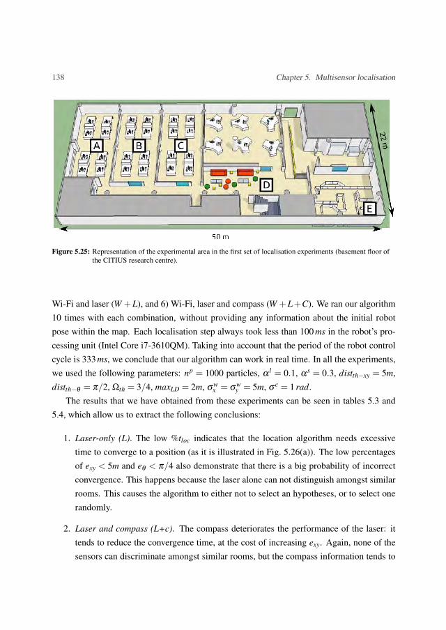
138 Chapter 5. Multisensor localisation
Figure 5.25: Representation of the experimental area in the first set of localisation experiments (basement floor ofthe CITIUS research centre).
Wi-Fi and laser (W +L), and 6) Wi-Fi, laser and compass (W +L+C). We ran our algorithm10 times with each combination, without providing any information about the initial robotpose within the map. Each localisation step always took less than 100 ms in the robot’s pro-cessing unit (Intel Core i7-3610QM). Taking into account that the period of the robot controlcycle is 333 ms, we conclude that our algorithm can work in real time. In all the experiments,we used the following parameters: np = 1000 particles, α l = 0.1, αs = 0.3, distth−xy = 5m,distth−θ = π/2, Ωth = 3/4, maxLD = 2m, σw
x = σwy = 5m, σ c = 1 rad.
The results that we have obtained from these experiments can be seen in tables 5.3 and5.4, which allow us to extract the following conclusions:
1. Laser-only (L). The low %tloc indicates that the location algorithm needs excessivetime to converge to a position (as it is illustrated in Fig. 5.26(a)). The low percentagesof exy < 5m and eθ < π/4 also demonstrate that there is a big probability of incorrectconvergence. This happens because the laser alone can not distinguish amongst similarrooms. This causes the algorithm to either not to select an hypotheses, or to select onerandomly.
2. Laser and compass (L+c). The compass deteriorates the performance of the laser: ittends to reduce the convergence time, at the cost of increasing exy. Again, none of thesensors can discriminate amongst similar rooms, but the compass information tends to

5.7. Experimental results 139
Traj.1L L+ c W W + c W +L W +L+ c
µ σ µ σ µ σ µ σ µ σ µ σ
exy (m) 1.81 2.25 2.67 2.88 2.72 0.30 2.54 0.36 0.77 0.38 0.52 0.15eθ (rad) 0.14 0.18 0.07 0.02 0.25 0.05 0.12 0.03 0.15 0.12 0.08 0.02
exy < 5m (%) 87.5 18.2 76.5 23.0 93.4 2.37 98.6 0.07 97.6 3.45 99.3 0.00eθ < π/4 (%) 97.8 5.80 100 0.00 95.0 3.50 98.3 0.67 97.2 0.45 99.8 0.06
tloc (%) 74.4 15.6 79.9 7.7 76.6 6.4 87.0 3.68 84.2 2.63 93.3 2.18
Table 5.3: Results for trajectory 1 on the first set of experiments. We provide averages (µ) and standard deviations(σ ) of: error in position (exy) and orientation (eθ ), percentage of time that the error in position is below 5meters, percentage of time that the error in orientation is below π/4 rad, and percentage of time that thealgorithm is able to provide a localisation estimation (tloc). Bolded numbers highlight the best results.
Traj.2L L+ c W W + c W +L W +L+ c
µ σ µ σ µ σ µ σ µ σ µ σ
exy (m) 0.42 0.44 5.65 5.77 1.22 0.42 1.83 0.71 0.92 0.61 0.59 0.30eθ (rad) 0.14 1.68 0.07 0.05 1.80 0.57 0.17 0.06 1.62 1.37 0.18 0.11
exy < 5m (%) 100 0.00 44.4 52.7 100 0.00 99.0 2.23 100 0 100 0.00eθ < π/4 (%) 66.7 57.7 100 0.00 13.4 21.5 100 0.00 48.9 48.4 100 0
tloc (%) 13.9 25.2 41.0 25.3 45.1 15.9 70.2 18.6 60.4 13.6 80.6 4.59
Table 5.4: Results for trajectory 2 on the first set of experiments. We provide averages (µ) and standard deviations(σ ) of: error in position (exy) and orientation (eθ ), percentage of time that the error in position is below 5meters, percentage of time that the error in orientation is below π/4 rad, and percentage of time that thealgorithm is able to provide a localisation estimation (tloc). Bolded numbers highlight the best results.
reduce the diversity of particles. This increases the probability of convergence towardsa random hypothesis.
3. Wi-Fi only (W). It has high exy values, but the percentage of exy < 5m is also quite high.This means that even though Wi-Fi might not have a high accuracy in short distances itis very adequate to discriminate amongst spatially distant hypotheses. In the example,amongst the laboratories (A, B, C in Fig. 5.25) and the large corridor in our building.

140 Chapter 5. Multisensor localisation
(a) Poor localisation results when using only laser data.
(b) High localisation performance example when using all the sensors in our robot (laser, wifi and compass).
Figure 5.26: Two trajectory samples (grey line) generated with our localisation algorithm on the first set ofexperiments. The ground truth trajectory is represented with grey squares. Letters A and Z representthe start and end points, respectively, of the trajectory. Letter B represents the point where ouralgorithm starts to output a pose estimate, and the grey star represents the actual position of the robotat that moment. Letter C indicates a zone in Fig. 5.26(a) where our algorithm had to correct its poseestimate.

5.7. Experimental results 141
4. Trajectory 1 vs 2. If we compare the results obtained for the two trajectories, we cansee that the main difference is that %tloc is much higher in the first one. This happensbecause in the second trajectory the robot is just spinning, continuously obtaining thesame (or similar) sensor data, therefore the data is not discriminative enough to obtaina fast first estimate of the robot’s pose.
5. Wi-Fi and compass (W+c). The compass improves slightly the performance of the Wi-Fi. Noticeably, it reduces the percentage of eθ > π/4 to a 0%.
6. Wi-Fi and laser (W+L). The Wi-Fi helps the laser to discard spatially distant hypothe-ses. This improves %tloc, and increases the percentage of exy < 5. However, the Wi-Fiadds noise, which tends to increase the values of exy and eθ .
7. Wi-Fi, laser, and compass (W+L+c). This is the best combination, as we illustratein Fig. 5.26(b), which overcomes the drawbacks shown in Fig. 5.26(a). It shows apercentage of exy < 5 above the 99%, and a percentage of eθ < π/4 of 100%. Moreover,the high value of tloc (80.59% in trajectory 2 and 93.3% in trajectory 1), and the low σ
values indicate a fast and stable convergence (convergence time below 11 seconds).
Discussion of the first set of experiments
We have proved that the combination of information sources with non-correlated errors tendsto perform better than solutions based on single sensors alone [128]. It avoids the confusionbetween similar spaces, and it provides accurate localisation estimates. We have also testedsome of our observation models, and validated our multisensor fusion algorithm for robotlocalisation.
Although not reflected in the experimental data, we have observed that the WiFi obser-vation model can be improved. We have observed that sometimes the robot receives similarWiFi measurements in different areas of the environment. This causes the ε-SVR to predictthat the robot is in any of those areas almost randomly, which causes the robot estimate to“jump” continuously. This problem is not unique to ε-SVR, but to any regression method thataims to predict a single intermediate position. Instead, a method such as GP regression (Sec.5.5.2), that estimates the potentially multi-modal probability distribution of receiving a certainmeasurement zw
t across the whole environment might be more adequate for WiFi localisation.On the other hand, we have noted that the compass model works well in general, but there
are certain areas where the magnetic interferences are too strong and distort the measurements

142 Chapter 5. Multisensor localisation
completely. In this case, orientation values should be discarded, but the stationary model doesnot allow that. Therefore, we believe that a non-stationary model could improve the results inthese situations.
5.7.2 Laser, WiFi GP Regression, multi-camera network and compasswith non-stationary distortion
Again, we have deployed our system in the basement floor of the CITIUS research cen-tre. Figure 5.27 shows an sketch of the experimental area. We have used a Pioneer P3DXrobot equipped with a SICK-LMS100 laser, a Devantech CMPS10 magnetic compass, a CiscoWUSB54GCv3 Wifi USB card, 9 WiFi APs (not belonging to the building), and a network of5 Microsoft HD-5000 usb cameras (C1 to C5 in Fig. 5.27), each one connected to a laptop.Table 5.5 shows a summary of a calibration trajectory in this environment, which took lessthan 20 minutes. Figs. 5.28-(a) and 5.28-(b) show two training sets gathered to calibrate theWiFi and the cameras following our methodology (respectively). Figure 5.29 shows the resultof the WiFi calibration, and Fig. 5.30 the result of the camera calibration.
This time, we have performed a total of four localisation experiments, each reflectingdifferent common situations of robot operation in environments where people works and lives.In experiment 1 (trajectory 1, Table 5.5) the robot moves within an area that is very similar to
Figure 5.27: Representation of the experimental area on the second set of experiments. Tags A, B, C, D and Ecorrespond to relevant zones (see Sec. 5.7) Tags C1, C2, C3, C4, and C5 represent the locations of thecameras. We also show the APs position and the cameras FOV.

5.7. Experimental results 143
Trajectory Length Odometry Laser WiFi Cameras CompassCalibration 1148s/646m 11462 56334 841 109 11483
1 198s/76m 1972 9830 137 29 19792 185s/65m 1857 8271 128 27 18583 110s/40m 1100 5476 76 38 11014 87s/27m 703 3492 60 20 8725 133s/50m 1331 6644 92 9 13316 90s/25m 908 4513 62 16 907
Table 5.5: Summary of each trajectory in the second set of experiments: length (in seconds and meters), andnumber of readings of odometry, laser, WiFi, cameras (cams), and compass.
(a) (b)
Figure 5.28: Calibration points recorded on the setup of the second set of experiments: a) WiFi, b) network ofcameras (each camera is shown with a different colour).
others (environment symmetries). In experiment 2 (trajectory 2, Table 5.5), we have analysedthe impact on our algorithm of several furniture rearrangements (environment changes). Inexperiment 3 (trajectories 3 and 4, Table 5.5) the robot was following a group of persons(group following). Finally, experiment 4 (trajectories 5 and 6, Table 5.5) was performedduring a real robotics demonstration in front of visitors (crowded environment).
In all the localisation experiments, we have used the following parameters: np = 4000 par-ticles, α l = 0.1, αs = 0.3, distth−xy = 5m, distth−θ = π/2, Ωth = 3/4, maxLD = 2m, λ c = 1,λ w = 4. We have executed our algorithm with a period of 333 ms (control cycle), enough toensure correct performance of the tasks carried out by our robot (e.g. planning and naviga-tion). The execution of the localisation algorithm takes approximately 30 ms of the control

144 Chapter 5. Multisensor localisation
Figure 5.29: Average power (in absolute dBms) of each WiFi AP computed from the data captured during the setupof the second set of experiments. The lower (red), the more powerful. The higher (blue), the lesspowerful.
Figure 5.30: Camera maps MC computed from the calibration data captured during the second set of experiments.A high likelihood (blue) indicates camera coverage. From left to right, we show the maps of camerasC1, C2, C3, C4, and C5 (see Fig. 5.27).
cycle (less than in the previous experiment, due to code optimisation). This indicates that ouralgorithm can work in real time.
Experiment 1. Environment similarities.
The first experiment corresponds with the trajectory shown in Fig. 5.31. Figs. 5.31-(a) and5.31-(b) show the ground truth and represent the error at each position when using only laseror the combination of all the sensors (respectively). In addition, Figs. 5.31-(c), 5.31-(d), and5.31-(e) show the performance boxplots for the 3 sensor combinations mentioned before.

5.7. Experimental results 145
We observe that the laser was useless during this experiment: it is not able to convergemost of the time, and when it does the error is extremely high. This happens because thetrajectory is confined only to room A, which is very similar to rooms B and C (see Fig. 5.27).Indeed, the algorithm chooses randomly among these rooms when it uses only the the laserinformation.
On the contrary, we observe that using all the sensors improves dramatically the results.This happens because the WiFi and the cameras break the influence of the similarity amongthe rooms.
Experiment 2. Changes in the environment.
The second experiment corresponds with the trajectory in Fig. 5.32. This trajectory is evenmore challenging, because we have rearranged the layout of the sofas and tables of area D(Fig. 5.27). Again, the experimental results show that the laser is useless on its own: sincewe have changed the environment, the signature of the laser can not match to the signatureexpected from the map. The fusion of all the sensors improves the results. Note that in thiscase, the combination W+C+c outperforms the rest. This indicates that the laser is introducingsevere errors. However, the fusion of all the sensors is able to mitigate them.
Experiment 3. Group following.
The third experiment corresponds to two trajectories, one of which is shown in Fig. 5.33 (theother is similar, but in an opposite direction). These trajectories are ideal for the laser, becausethe robot traverses very different areas, which mitigates the errors derived from similaritiesin the environment. During the trajectories the robot was following a person, while otherfour were walking by the robot (see Fig. 5.34-(a)). This is a typical situation for our guide-tour robot [129]. We expected that the legs of the people around the robot would distortsignificantly the laser signatures.
Figure 5.33 shows the experimental results when the robot follows these trajectories. Theaccuracy of the laser is very high, therefore we conclude that the presence of small groups ofpeople do not lead to failure when using the laser alone. On the one hand, this indicates that asubstantial part of the laser signature still contains valid information, despite of the occlusion.On the other, this demonstrates the robustness of the laser observation model that we havesuggested. Given the good performance of the laser alone, the main contribution of the sensorfusion is the reduction of the convergence time (Fig. 5.33-(c)). This is because the laser alone

146 Chapter 5. Multisensor localisation
(a) exy (meters): L
(b) exy (meters): L+W+C+c
(c) exy (meters) (d) tconv (seconds) (e) %tloc−conv (percentage)
Figure 5.31: Results of the trajectory of experiment 1 from the second set of experiments (Sec. 5.7.2). a-b) Colourred represents exy ≥ 3m, and colour green represents exy < 3m. c-d-e) exy, tconv and %tloc boxplots forthe sensor combinations (L+W +C+ c, L and W +C+ c).

5.7. Experimental results 147
(a) exy (meters): L
(b) exy (meters): L+W+C+c
(c) exy (meters) (d) tconv (seconds) (e) %tloc−conv (percentage)
Figure 5.32: Results of the trajectory of experiment 2 from the second set of experiments (Sec. 5.7.2). a-b) Colourred represents exy ≥ 3m, and colour green represents exy < 3m. c-d-e) exy, tconv and %tloc boxplots forthe sensor combinations (L+W +C+ c, L and W +C+ c).

148 Chapter 5. Multisensor localisation
(a) exy (meters): L
(b) exy (meters): L+W+C+c
(c) exy (meters) (d) tconv (seconds) (e) %tloc−conv (percentage)
Figure 5.33: Results of the trajectory of experiment 3 from the second set of experiments (Sec. 5.7.2). a-b) Colourred represents exy ≥ 3m, and colour green represents exy < 3m. c-d-e) exy, tconv and %tloc boxplots forthe sensor combinations (L+W +C+ c, L and W +C+ c).

5.7. Experimental results 149
(a) (b)
Figure 5.34: a) Picture taken while the robot is following a person and other four people walk nearby (experiment 3of the second set of experiments , Sec. 5.7.2). b) Picture taken while the robot is moving in a crowdedarea during a robotics demonstration (experiment 4 of the second set of experiments , Sec. 5.7.2)
can not converge while moving inside room A due to its similarities with rooms B and C, aswe have seen in Sec 5.7.2.
As a curiosity, in Fig. 5.33-(b) we see that the error of sensor fusion grows after theconvergence always in the same region. We have observed that this is due to errors introducedby the compass, due to very strong magnetic interferences in that area (see Fig. 5.20).
Experiment 4. Crowded environment.
This experiment corresponds with two trajectories, one of which is shown in Fig. 5.35 (theother one is similar). We have carried out this experiment while the robot was operatingin a real social event (Fig. 5.34-(b)). We have recorded the trajectories during a roboticsdemonstration in front of 20 external visitors approximately. Some visitors were movingaround the robot in different directions, others were standing still alone or in groups, etc.Therefore, we would expect that they would occlude the laser with their legs significantly.
The results of this experiment are shown in Fig. 5.35. First of all, we observe a cleardifference between the performance of the laser in this experiment and the previous one (Sec.5.7.2). In the previous experiment, the moderate presence of people did not affect the lasersignificantly. However, the current experiment shows that the density of people that we mightfind in real situations does affect the laser performance in terms of accuracy, convergence

150 Chapter 5. Multisensor localisation
(a) exy (meters): L
(b) exy (meters): L+W+C+c
(c) exy (meters) (d) tconv (seconds) (e) %tloc−conv (percentage)
Figure 5.35: Results of the trajectory of experiment 4 from the second set of experiments (Sec. 5.7.2). a-b) Colourred represents exy ≥ 3m, and colour green represents exy < 3m. c-d-e) exy, tconv and %tloc boxplots forthe sensor combinations (L+W +C+ c, L and W +C+ c).

5.7. Experimental results 151
time and stability. In fact, the part of the trajectory in Fig. 5.35-(a) where the error is highercorresponds to the area shown in Fig. 5.34-(b), where there are many people around therobot. On the other hand, during the rest of the trajectory there were no people around therobot. Finally, we observe that the fusion of all the sensors works very robustly even in thesechallenging situations. The algorithm converges very fast, it is very stable and the errors arevery low.
Discussion of the second set of experiments
In Fig. 5.36 and Table 5.6 we show the average and standard deviation of the performance ofthe system for every metric (exy, eθ , tconv, %tloc). We have considered each sensor combina-tion and we have used the data from all the experiments. On the other hand, in Table 5.7 werank the performance (with statistical significance) of each sensor combination. Consideringthese results, we can conclude that the best combination is laser, WiFi, cameras, and compass(L+W+C+c), since it is the only one that is among the bests in all the categories. Moreover,we can draw the following conclusions:
– The WiFi tends to produce reasonably good results in terms of position accuracy, con-vergence time and stability. For instance, it is always present in the combinations thatmaximise %tloc (Table 5.7). Since the WiFi does not provide orientation information,the orientation accuracy is poorer (although acceptable in most cases). Overall, it hasproven to be a very robust and stable information source.
– The cameras (C) are always present in the combinations that minimise the tconv (Table5.7). On the other hand, they seem to perform worse than the WiFi in position andorientation error and stability. However, experiments have shown that only the stabilitydifferences are significant. Nevertheless, we believe that a wider experimental analysiswould have pointed out accuracy differences among them. This is because, on the onehand, the cameras are the sensors that provide less information. This happens becausethey provide information at a lower rate, the presence of people occludes the robot, andthe range of detection is limited to 15 meters in practice. On the other hand, the WiFiAPs have bigger ranges which overlap significantly, providing redundancy. Moreover,the presence of people affects the WiFi less than the cameras.
– The laser alone performed poorly because of its inability to deal with symmetries,changes in the environment, and crowded spaces. On the other hand, we have found

152 Chapter 5. Multisensor localisation
out that the laser works well when: a) the trajectory is sufficiently large and diverse, b)there is few or no people around the robot.
– The compass improves the orientation accuracy. The robotics community tends to as-sume that a compass can not be used for robot localisation, because of the magneticinterferences of the environment [64, 31]. However, we have demonstrated that even alow cost compass can be used if we model adequately the magnetic interferences of theenvironment (Sec. 5.5.3). On the other hand, the compass may cause errors in areaswhere the magnetic interference is very strong (see Fig. 5.20). Nevertheless, this shouldbe solved with a finer adjustment of the compass model.
(a) exy (meters) (b) eθ (radians)
(c) tconv (seconds) (d) %tloc−conv (percentage)
Figure 5.36: Boxplots of the performance of the localisation in all the experiments of the second set with differentsensor combinations.
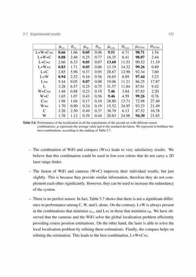
5.7. Experimental results 153
µexy σexy µeθσeθ
µtconv σtconv µ%tloc σ%tloc
L+W+C+c 0.66 1.66 0.05 0.06 9.51 6.71 98.71 1.54L+W+C 0.88 2.46 0.25 0.77 16.35 8.41 98.07 2.44L+C+c 2.66 6.33 0.05 0.07 13.60 11.53 90.52 11.19L+W+c 0.83 1.71 0.05 0.06 13.19 14.32 99.26 0.89
L+C 2.85 5.96 0.37 0.95 28.67 12.90 92.34 7.60L+W 0.94 2.52 0.16 0.56 18.65 8.89 97.44 3.23L+c 5.44 9.05 0.07 0.08 19.06 11.21 86.25 17.87
L 3.28 6.57 0.25 0.75 31.57 11.84 87.61 9.42W+C+c 1.48 0.88 0.23 0.19 7.46 3.84 97.82 2.20
W+C 1.65 1.07 0.43 0.56 9.46 4.59 99.26 0.76C+c 1.98 1.04 0.17 0.10 28.80 13.71 72.98 27.40W+c 1.70 0.90 0.24 0.19 15.52 24.95 93.23 21.49
C 3.26 2.50 0.49 0.37 38.79 6.13 87.52 16.78W 1.76 1.12 0.39 0.44 20.83 24.96 94.30 21.65
Table 5.6: Performance of the localisation in all the experiments of the second set with different sensorcombinations. µ represents the average value and σ the standard deviation. We represent in boldface thebest combinations, according to the ranking of Table 5.7.
– The combination of WiFi and compass (W+c) leads to very satisfactory results. Webelieve that this combination could be used in low-cost robots that do not carry a 2Dlaser range finder.
– The fusion of WiFi and cameras (W+C) improves their individual results, but justslightly. This is because they provide similar information, therefore they do not com-plement each other significantly. However, they can be used to increase the redundancyof the system.
– There is no perfect sensor. In fact, Table 5.7 shows that there is not a significant differ-ence in performance among C, W, and L alone. On the contrary, L+W is always presentin the combinations that minimise exy, and L+c in those that minimise eθ . We have ob-served that the cameras and the WiFi solve the global localisation problem efficientlyproviding coarse position estimations. On the other hand, the laser is able to solve thelocal localisation problem by refining these estimations. Finally, the compass helps onrefining the orientation. This leads to the best combination, L+W+C+c.

154 Chapter 5. Multisensor localisation
– The algorithm performs correctly with any subset of sensors available, even if they workat different rates or if they stop working: if a sensor is not available, the performancejust degrades gracefully.
exy eθ tconv %tloc−conv
Ranking
L+W+C+c L+W+c L+W+C+c W+CL+W+c L+C+c W+C WL+W+C L+W+C+c W+C+c L+W+c
L+W L+c L+C+c L+W+CW+C+c L+W+C L+W+c L+WL+C+c C+c W+c L+W+C+c
W L+W L+W+C L+CW+C W+C+c C+c W+C+cW+c W+c L+W W+cL+C L+C C L+cL+c C W L+C+c
L W+C L+C C+cC W L+c L
C+c L L CFriedmanAlignedRanksp-value
0.00017 0.0000017 0.00020 0.0072
Holmp-value 0.00000020 0.000000019 0.00039 0.000034
Table 5.7: Ranking of each sensor combination according to different statistical measurements using the FriedmanAligned Ranks method [130]. We highlight in boldface the best combinations. We separate combinationswith horizontal rows when there is a significant different among them (post-hoc Holm test [130] withα = 0.05). These statistical tests were performed using the STAC web tool [131]. The Holm p-valuerefers to the adjusted p-value of the first combination of the ranking that performs significantly worsethan one of the best group.
5.7.3 Scene recognition
In this experiment, we have analysed the performance of scene recognition in mobile robotpositioning. To have a baseline for comparison, we have also analysed the performance ofother sensors in the experiment: laser, WiFi with GP regression, compass with non-stationarydistortion, and a network of cameras. We have performed 2 experiments at the CITIUS re-

5.7. Experimental results 155
search building, one in the basement floor and one in the ground floor. We have used a PioneerP3DX robot equipped with a SICK-LMS100 laser, a Devantech CMPS10 magnetic compass,a Kinect camera, a laptop with Wi-Fi connectivity (Intel Core i7-3610QM @ 2.3GHz, 6GBRAM), 5 WiFi APs, and a network of 5 Microsoft HD-5000 USB cameras (each one con-nected to a laptop). We have established a period of 1000ms (control cycle) to execute ouralgorithm.
In this experiment, we have followed a methodology similar to other experiments. First,we have moved the robot along the environment following different trajectories and collectingall sensors information (training data sets). Then, we have run the localisation algorithm overthe trajectories with different the sensor combinations (10 times with each combination). Wehave considered the error in position exy, the convergence time tconv, and the stability tloc−conv
of the algorithm. To explain the experiments, we will use L to refer to the laser, W to the WiFipositioning, C to the cameras, c to the compass and K to the Kinect with scene recognition.
Both experiments took place at the basement and ground floor of the CITIUS building(Fig. 5.37), respectively. Figure 5.38 shows the performances achieved with all the sensorcombinations in the first experiment, and Fig. 5.39 the performances achieved in the secondexperiment. We are mainly interested in combinations that include the Kinect sensor but wealso show the performance of the localisation system achieved with other sensors.
It is interesting to study how Kinect sensor works compared to Wi-Fi or the network ofcameras, since all of them provide a probability grid for the localisation system. As we can seein Fig. 5.38-(a), Kinect has a slightly worse performance to sensors such as WiFi positioningand the network of cameras when looking at exy and tloc−conv. However, the convergence timestconv of Kinect are significantly worse than those of WiFi and cameras. This result is directly
(a) (b)
Figure 5.37: Occupancy maps created using GMapping SLAM algorithm for the third set of experiments: a)basement floor map, b) ground floor map.

156 Chapter 5. Multisensor localisation
Figure 5.38: Results of the basement floor experiment from the third set of experiments: a) exy, b) tconv, c) tloc−conv.
Figure 5.39: Results of the ground floor experiment from the third set of experiments: a) exy, b) tconv, c) tloc−conv.
related to the accuracy of the image classifier (88% success rate in these experiments [122]).Even more, the convergence time of Kinect in the basement floor (Fig. 5.38) is significantlyworse than in the ground floor, because this last environment is much more diverse and thereexist less symmetries, therefore the classifier performs more robustly and accurately.
The combination W+K shows how WiFi and Kinect work together. The result reveals thatthey provide a similar information and, therefore, their combination does not achieve betteraccuracy. However, the combination always improves the stability. Finally, the performancewhen grouping many sensors together (e.g. like L+W+C+c+K or L+W+C+K), includingKinect as part of the system, improves slightly the accuracy in pose estimation and timerequired to get the first robot pose. Similarly, the stability is always improved when combiningsensors.

5.8. Discussion 157
These experimental results show that scene recognition can be used for mobile robot lo-calisation. Moreover, once more the experiments show how adding information sources canimprove the robustness of the positioning system.
5.8 Discussion
In this chapter, we have presented a localisation algorithm based on particle filters that fusesthe information of several sensors of different natures. Our algorithm is able to fuse bothon-board and external sensors, even if they are not synchronised or work at different datarates. Our algorithm is scalable (able to handle a variable number of sensors) and highlyparallelisable. We have demonstrated the use of this algorithm with multiple sensors, and wehave suggested one or more probabilistic observation models for each of them:
– 2D laser range-finder: we have suggested a model that takes into account the differencesbetween the expected and received laser signature, both regarding their shape and eachof their concrete values.
– Magnetic compass: we have suggested a model that takes into account the magneticdistortions present in the environment. This allows us to minimise their influence in theorientation readings.
– WiFi receiver card: we have suggested three different techniques that allow us to pin-point the position of the robot using the signal power received from the WiFi APs in theenvironment.
– Camera network: we have designed a model that is able to estimate the position of therobot based on the list of cameras that detect it at each instant.
– Camera on-board of the robot: we have developed a model based on scene recognitiontechniques, that allows us to estimate the most probable robot position from an imagetaken by the camera.
We have also demonstrated how to calibrate each sensor model with few data withoutoverfitting (context of fast deployment). The algorithm, the methodology, the mapping strat-egy and the probabilistic modelling can be extended to other sensors as well.
The suggested methodology was designed taking into account the casuistry of servicerobots (particularly, tour-guide robots). Our robots learn informative routes by following

158 Chapter 5. Multisensor localisation
an instructor around. During this process, the robot maps the whole working environment,so the mapping does not add much overhead to the deployment. Moreover, if we wantedto deploy not one but many similar robots, all of them could use same calibration models(at least theoretically), therefore the calibration effort would not increase. Nevertheless, webelieve that automatic exploration would be a nice feature to have. The robot could explorethe environment on its own or supported by the cameras [132, 133] prior to the route learningprocess. Even more, we could explore hybrid alternatives, where the robot would be able tocomplete the mapping directed by the instructor with autonomous exploration.
We have performed experiments in both controlled and real operation conditions. Wehave demonstrated that our system can be deployed in a fast and easy manner even by nonexpert users. Moreover, experiments have shown that our system is able to cope with differentchallenges typical of social environments: a) people walking by the robot, b) crowded envi-ronments, c) changes in the environment, and d) similarities among different areas. We haveseen that there are two main kinds of sensors: a) those that provide rough global estimatesof the robot position, and b) those that provide precise local estimates. With sensors of thefirst group, the robot will receive an estimation of its position almost guaranteed, although itmight not have the highest precision. On the contrary, with sensors of the second group, therobot might be subject to temporary loses, although the precision of the estimation is usuallyhigher than with the first group. With statistical significance, we can affirm that the robustnessof the system increases as more sensors are fused (specifically when fusing sensors from bothgroups). In fact, the fusion of all the sensors is always among the top performers for all theparameters analysed (with statistical significance). Finally, we have demonstrated that ouralgorithm performs correctly with any subset of sensors available, even if they work at differ-ent rates or if they stop working: if a sensor is not available, the performance just degradesgracefully.
With this in mind, it is clear that our system no longer depends exclusively on the informa-tion of the multi-camera network. Now, the robot can localise itself and navigate without theirhelp, that is, it can be a “smart” robot. However, this approach is not perfect either, becausethe system depends completely on the occupancy map that we generate at deployment time.There will be situations where we might not be able to build such a map accurately, at least incertain areas (e.g. in environments with slippery floors where the robot wheels might slide).In this case, the external cameras can still be used to support the robot navigation, even if the

5.8. Discussion 159
localisation algorithm can not work momentarily or during the whole operation. Moreover,the cameras will still be used to detect situations of interest to which the robot should attend.


CHAPTER 6
WIRELESS LOCALISATION WITH VARYING
TRANSMISSION POWER
In this thesis, one of our objectives is to be able to deploy robots in different environments,in a fast and easy manner. We have seen that having a robust localisation system is importantwhen we want our robots to perform their tasks correctly. In the previous chapter, we havedemonstrated the potential of WiFi positioning, specifically when combined with other sen-sors, such as 2D laser range-finders. In this chapter, we will explore a more flexible wirelesspositioning alternative.
WiFi transmitters used in WiFi positioning systems are mostly commercial. Therefore,they use similar transmission powers that can not be modified. We consider that the use oftransmitters that can vary their transmission power could lead to a number of benefits. Onthe one hand, each environment is different, and using a default transmission power may notbe the most optimum solution. On the other, different parts of the environment or differentsituations might require different levels of accuracy and robustness, and therefore differenttransmission powers. For instance, the signal attenuation of a high power transmitter mightnot be noticeable in a small room, so it might not be possible to distinguish where the robotis within the room. On the contrary, a low power transmitter might not be received out ofa region close to it, so we could know whether the robot is within this region. Even more,different transmission powers lead to different signal propagations, which provide differentinformation. Therefore, the use of transmitters with varying transmission power will increasethe discrimination ability of the localisation system. In the extreme, these transmission pow-

162 Chapter 6. Wireless localisation with varying transmission power
ers could be changed by the robot itself. This would allow the robot to discard localisationhypotheses actively depending on different criteria: the quality of the current localisation es-timate, the task at hand, the part of the environment where the robot is, etc. In fact, the abilityof the robot to change the transmission power of the motes would be more profound than that.This ability would take us back to the collective intelligence paradigm: now, not only theintelligent environment would be able to modify the robot behaviour, but the robot would beable to change the way the environment works as well. Taking this into account, in this thesiswe will explore the use of wireless transmitters that are able to vary their transmission power.
In this chapter, we describe the wireless motes that we have designed in the context of thisthesis, and how we have integrated them into our localisation algorithm (Sec. 6.1). After that,in Sec. 6.2 we describe the experiments that we have carried out in order to test whether ornot varying the transmission power increases the quality of wireless positioning systems.
6.1 Wireless sensor nodes (motes) for mobile robot localisation
In this thesis, we will use specifically designed wireless sensor nodes [134, 135], also knownas motes. We could have used other alternatives, such as commercial WiFi APs or Bluetoothbeacons, but motes are a flexible and convenient solution for our purposes. Moreover, moteshave several characteristics that make them very appealing for mobile robot applications:
– Control over the software and hardware of the mote. This enables the adjustment of thetransmission power, among other properties.
– Communication capabilities. Motes can be used for communication among robots andenvironment elements.
– Low power consumption. Motes usually consume much less power that their WiFi APs.What is more important, designers have full control over it.
– Homogeneous hardware. It is known that different WiFi receptors have different recep-tion properties, which constitute a challenge for wireless localisation algorithms [136].Having homogeneous hardware limits this phenomenon, and simplifies the workingconditions of the robots, which enhances the robustness and reduces the cost of designand deployment.

6.1. Wireless sensor nodes (motes) for mobile robot localisation 163
– Several frequency bands. This might be interesting if we want to avoid interferenceswith existing systems (such as WiFi networks), or to comply with radiation policies ofthe application environment (e.g. in hospitals or industrial plants).
We have designed and developed motes with the help of Dr. Jose Manuel Rodríguez As-cariz, from the University of Alcalá. Our motes use a CC1110 SoC (Fig. 6.1-(a)), that com-bines an industry-standard enhanced 8051 MCU and an excellent performance RF transceiverCC1101 that operates in the 433 MHz band. These motes can be produced for less than 15 eeach, allow the modification of several transmission parameters, and have a very small powerconsumption. More concretely, our motes operate at 3V and consume less than 10 uA in sleepmode, 34 mA when transmitting at 10 dBm (maximum power), and 0.1 mA when configuredfor our robot localisation purposes (assuming a 2 ms data burst every 1 s at maximum trans-mission power, 10 dBm). Therefore, they consume approximately 0.1W in the worst case,and 0.1 mW in a typical setting. Just to give a comparison, we have measured that the powerconsumption of a commercial router (Linksys WAG200G) is 4.5W even when it is not trans-mitting information. Every mote is powered by two AAA batteries with an estimated batterylife of several months in a typical setting. We have programmed the motes to operate at a 10kbps data rate, using GFSK modulation in the 433 MHz ISM band with 19 kHz of deviationand 100 kHz of RX bandwidth filters.
(a) (b)
Figure 6.1: a) Prototype of a mote using a CC1110 sub-1GHz SoC with a monopole antenna. b) Radiation patternof the monopole antenna for an arbitrary transmission power.

164 Chapter 6. Wireless localisation with varying transmission power
We have equipped each mote with a 1.8 dBi monopole antenna from MaxStream (Fig.6.1-(a)). The radiation pattern of this antenna is illustrated in Fig. 6.1-(b). In the azimuthradiation graph, we observe that the antenna radiates equally in all the directions of the planeparallel to the ground. We will estimate the position of the robot in this plane (2D robotlocalisation). In the elevation radiation graph, we observe that the antenna also radiates indirections that are not parallel to the ground. Therefore, in principle the motes could be usedto estimate the attitude of a receiver. For instance, they could distinguish among differentfloors, or the attitude of a drone, although this goes beyond the scope of this thesis. Moreover,in this last case other sensors (e.g. sonar sensors) could provide higher precision, becauseindoor ceilings are rarely high and the attenuation from the ground to the ceiling would notbe perceivable.
Our motes can be used both for communications and localisation purposes, but in this the-sis we will focus in the latter. In this regard, we have programmed some of the motes to senddata packages periodically (transmitter motes). The data sent in the packages indicates theoutput power at which the packages are transmitted, and the ID of the transmitting mote. Onthe other hand, the receiver motes were programmed to receive these packages and measurethe power of the signal received. These motes are placed on board of the robot.
Most of the positioning works with motes have been devoted to the localisation of thestatic motes that form the sensor network [137, 138]. There have been a few attempts to usemotes in person [139] and robot positioning applications [140, 31], but examples are scarce.Therefore, we will propose our own localisation system based on motes. More concretely, theobservation model of these motes will be the same used with the WiFi technology describedin Sec. 5.5.2 based on the GP Regression technique. Therefore, we do not need to make anychanges in the algorithm nor in the deployment methodology.
Figure 6.2 shows a representation of the functions µk(x,y) and σ k(x,y) for a sample mote.Figure 6.3 shows two examples of this likelihood distribution when the robot is at two differentpositions. Note that in both cases the distribution is multi-modal, but there is usually an areathat concentrates most of the likelihood.

6.2. Experimental results 165
(a) µwi (x,y) (b) σw
i (x,y)
Figure 6.2: Output of the GP regression for a sample mote. a) The lowest values (red) correspond to the highestpower. It is clear that the mote was located near the position (40m,16m). b) The lowest values (red)correspond to the lowest typical deviation power.
(a) (b)
Figure 6.3: Likelihood distribution provided by the mote observation model at two different positions (highestvalues in blue, lowest values in red).
6.2 Experimental results
The objective of these experiments is to test whether the use of varying transmission powersincreases the quality of a wireless robot positioning system. To these extent, we will performtwo different experiments:
1. Analysis of the performance of localisation with motes and WiFi localisation using afixed transmission power in both cases. We want to compare their performance to seewhether localisation with motes could be used in the context of mobile robot localisa-tion. It is known that the performance of WiFi localisation depends on the quality ofthe WiFi card attached to the robot [136]. Therefore, to obtain a more reliable result,we will perform this experiment by using 3 different WiFi cards.
2. Analysis of the performance of the localisation with motes when using different trans-mission powers. We will also explore if using motes that change their transmission

166 Chapter 6. Wireless localisation with varying transmission power
power dynamically increases the performance of the localisation algorithm. This is im-portant, because if this is the case, robots could change the transmission power of motesto achieve a better performance (e.g. active localisation, where the robot may ask themotes to modify the transmission power in order to validate or reject localisation hy-potheses).
We have performed experiments in two different floors of the CITIUS research centre(Centro Singular de Investigación en Tecnoloxías da Información da Universidade de Santiagode Compostela, Spain). We have deployed 6 WiFi Access Points and 6 motes at each floor(each mote was placed near to an AP, to achieve a fair comparison). The WiFi APs are TP-Link TD-W8968 with EIRP<20dBm (Equivalent Isotropically Radiated Power). These APshave 2 dipole antennas of 5dBi each, while each mote has a 1.8dBi monopole antenna (Sec.6.1). The radiation pattern of each WiFi antenna in the azimuth plane (the relevant in oursystem) is similar to the pattern of each mote antenna (Fig. 6.1). On the other hand, we haveused a Pioneer P3DX robot equipped with a SICK-LMS100 laser, 1 mote (receiver), and 3different commercial WiFi receiver cards.
To collect the experimental data, we have moved the robot around the environment with ajoystick. During this process, the robot recorded the information received from the odometryencoders, the laser, and the signal power received by the mote and the WiFi cards. Table 6.1shows a summary of the data collected, and Fig. 6.4 a representation of the trajectory followedby the robot. Note that one of our experiments involves changing the power transmission ofthe motes. In principle, we would have to repeat the data capture stage as many times asthe number of transmission powers that we would like to explore (re-configuring the motesevery time). Instead, we have programmed the transmission motes to send a new package ofdata each 250ms. Each package is transmitted with a different power: -40 dBm, -30 dBm,-20 dBm, -10 dBm, 0 dBm, 5 dBm, 7 dBm, and 10 dBm. Therefore, the first package istransmitted at -40dBm, after 250ms a new package is transmitted at -30dBm, and so on. The
Experiment Length Odometry Laser Motes WiFi0 WiFi1 WiFi21 2330s/878m 23245 115846 1150 1673 1691 11552 2894s/1245m 28898 144136 2756 2093 2108 1416
Table 6.1: Summary of each experimental trajectory: length (in seconds and meters), and number of readings ofodometry, laser, and WiFi.

6.2. Experimental results 167
(a)
(b)
Figure 6.4: Trajectory followed by the robot during the capture of the experimental data for localisation withvarying transmits power in the CITIUS building. a) Ground floor. b) First floor.
cycle is repeated after 2 seconds, after the package at 10 dBm is transmitted. On the otherhand, the robot’s mote receives this packages, and every 2 seconds it sends to the robot avector containing the signal power of the last packages received. This way, to analyse theperformance under a certain transmission power, we just have to discard all packages exceptthose transmitted at the power that we want to analyse. Moreover, this same data can be usedto analyse the performance when the transmission power changes periodically.
After the experimental data was captured, we divided it in two subsets:
– Training set. Represents approximately the first 33% of the data set. We used thisset to construct the map (with the laser and odometry information) and to calibrate theobservation models of the mote and the 3 WiFi cards (with the signal power receivedby each of them).

168 Chapter 6. Wireless localisation with varying transmission power
– Testing sets. The remainder of the data set was divided randomly in 20 parts of 120seconds each. Each part was used to test the performance of our localisation algorithm.
In each experiment, we execute the algorithm using each of all the test sets (20 times each,to carry out statistical analyses). In each execution, the robot starts with no knowledge aboutits pose (global localisation), until the algorithm converges to a pose estimate (tracking). Thelocalisation algorithm estimates the trajectory followed by the robot using the robot odometryand the signal power received from the WiFi APs or motes (depending on the case). Finally,we compare this trajectory with the real trajectory (ground-truth), in order to evaluate:
1. Error in position and orientation (exy and eθ ): difference between the pose estimatedby the algorithm and the ground-truth (the lower the better).
2. Convergence ratio (%tloc): percentage of time that the algorithm provides an estimationof the pose (the higher the better). We consider that the algorithm has converged whenthe clustering step discovers a sufficiently important cluster of particles (Sec. 5.4.2).
We have always used the following parameters: np = 2000 particles, αs = 0.01, α f = 0.1,distth−xy = 5m, distth−θ = π/2, Ωth = 3/4. We have executed our algorithm with a period of333 ms (control cycle), enough to ensure the correct performance of the tasks carried out byour robot (e.g. planning and navigation). The execution of the localisation algorithm takesapproximately 15 ms of the control cycle. This indicates that our algorithm can work in realtime.
6.2.1 Results - Performance of motes vs. WiFi at a fixed transmissionpower
In this experiment, we have analysed the performance of the localisation algorithm usingmotes and WiFi APs at a fixed transmission power (we have used the same power for motesand WiFi APs). As we have explained, the performance of WiFi localisation depends on thequality of the WiFi card attached to the robot, so we will use 3 different WiFi cards in thisexperiment. Figure. 6.5 shows the radio maps of one floor, for each receiver. We can seethat the radio maps depend greatly on the hardware of the receiver [136]: each radio map isdifferent from the rest, not only between motes and WiFi, but among the 3 WiFi receivers aswell.

6.2. Experimental results 169
Figure 6.5: Radio maps generated with one of the data sets.
Figure 6.6 shows the performance results of the localisation with motes and WiFi. Theexperiments were performed using different values of the parameter λ w. This parameter scalesthe typical deviation estimated by the GP regression (Eq. 5.35). Therefore, it modifies theconfidence that we have in the sensor model (the greater the λ w, the lower the confidence andthe higher the tolerance towards noise). We can draw the following conclusions:
1. Higher values of λ w tend to give better results. On the one hand, this happens becauseparticle filters work better when they are conservative about the confidence put in ob-servation models [63]. On the other, the training data was captured during a limitedamount of time under very stable circumstances. Therefore, any regression algorithmwill tend to over-fit, but the λ w parameter helps to mitigate this problem. However, thevalue of the parameter can not be arbitrarily large: the larger λ w, the less informationthe observation model provides. Results show that the best trade-off is a value of λ w
between 3 and 4.
2. WiFi localisation results depend greatly on the hardware that we use: we have obtainedvery different results with each WiFi receiver.
3. Performance results of localisation with motes are at least as good as the best resultsof WiFi localisation. Therefore, our proposal is just as valid as WiFi localisation to beused for wireless robot localisation.

170 Chapter 6. Wireless localisation with varying transmission power
(a) exy
(b) eθ
(c) %tloc
Figure 6.6: Comparisson of the performance of the algorithm using the motes (blue) and each WiFi card (yellow,green, red) with fixed transmission power.

6.2. Experimental results 171
6.2.2 Results - Varying the transmission power
In this experiment, we have compared the performance of the localisation algorithm using:1) motes with different transmission powers, 2) motes that change the transmission powerperiodically, and 3) the best WiFi receptor of the previous experiments, whose transmissionpower can not be modified. In this case, we could only use 4 out of the 6 total transmittermotes, because the other 2 did not allow us to change the transmission power due to firmwarerestrictions. Obviously, we used only the 4 WiFi APs that were near the selected motes, toensure a fair comparison.
Note that we did not have to repeat the data capture stage, because the motes were alreadysending a new package of data each 250ms, each package with a different power (-40 dBm,-30 dBm, -20 dBm, -10 dBm, 0 dBm, 5 dBm, 7 dBm, and 10 dBm). Therefore, to analyse theresults with a certain fixed transmission power, we just have to discard all the packages, exceptthose transmitted with that power. Similarly, to analyse the results with a varying transmissionpower, we can consider that we have 8 “virtual” motes for every real mote (because eachreal mote transmits at 8 different powers per cycle). Therefore, to analyse the performancewhen varying the transmission power, we have trained a total of 32 “virtual” observationmodels, and we have just integrated each mote package using the observation model of itscorresponding “virtual” mote.
Figure 6.7 shows the performance results in this experiment, and Table 6.2 ranks theperformance of each configuration. The experiments were performed using a values of λ w.We can draw the following conclusions:
1. The best configuration is always the one that uses varying transmission power, and thedifference is significant when considering exy and eθ . This suggests that the use ofvarying transmission powers provides useful information that improves the localisationresults. This opens the door for future improvements in the line of active localisation.Under this paradigm, the robot would be able to modify the transmission power of themotes in order to discard localisation hypotheses proactively.
2. The second best configuration is, in this case, the one obtained when using the WiFicard. This contradicts partially the results obtained in the previous section, where themotes performed just as good as the best WiFi card. Nevertheless, just as in the pre-vious case, the results may vary depending on a number of factors: number of APs,distribution in the environment, environmental conditions, etc.

172 Chapter 6. Wireless localisation with varying transmission power
(a) exy
(b) eθ
(c) %tloc
Figure 6.7: Comparison of the performance of the algorithm using: a) motes with different fixed transmissionpowers (tagged as -30 dBm, -20 dBm, -10 dBm, 0 dBm, 5 dBm, 7 dBm, or 10 dBm), b) motes thatchange their transmission power periodically (tagged as All), and c) the WiFi card that performed betterin the previous experiment (tagged as WiFi1). We have discarded the results obtained when using atransmission power of -40 dBm, because the algorithm did not converge most of the times.

6.3. Discussion 173
Ranking exy eθ %tloc1 (best) All All All
2 WiFi1 WiFi1 WiFi13 0dB 7dB 7dB4 5dB -10dB 10dB5 7dB 10dB 0dB6 -10dB 5dB 5dB7 10dB 0dB -10dB
8 (worst) -20dB -20dB -20dB
Table 6.2: Ranking of the second experiment according to different statistical measurements using the FriedmanAligned Ranks method [130] (p− value = 0.05). We highlight in boldface the winning configuration.We separate configurations with horizontal rows when there is a significant different among them(post-hoc Holm test [130] with α = 0.05). These statistical tests were performed using the STAC webtool [131]. We have analysed performance of the algorithm using the motes with different transmissionpowers (tagged as -20 dBm, -10 dBm, 0 dBm, 5 dBm, 7 dBm, and 10 dBm), with varying transmissionpower (tagged as All), and with the best WiFi card of the previous experiment (tagged as WiFi1). Wehave discarded the results obtained when using a transmission power of -40 dBm (because the algorithmdid not converge most of the times) and -30 dBm (because the algorithm did not converge sometimes).
3. There is no significant difference among the different transmission powers analysed,considering exy and eθ . However, powers above 0 dBm perform better on the con-vergence rate results (%tloc). This makes sense, because motes with low transmissionpower can only be received in the surroundings of the mote. Therefore, the algorithmwill only converge when passing near one of them. We can extract two recommen-dations from these results. First of all, motes should use a transmission power of 0dBm, which is the lowest one with the best results. Second, lower transmission powersmight be used as well (e.g. proximity based localisation), but a greater number of motesshould be used.
6.3 Discussion
We have demonstrated that the use of transmitters with varying transmission powers can im-prove the performance of wireless positioning systems. We have proven this result with awireless localisation system for mobile robots. In particular, we have designed a system basedon motes that operate in the 433 MHz band. The motes allow to modify several transmissionparameters, and have a very small power consumption. We have presented the hardware and

174 Chapter 6. Wireless localisation with varying transmission power
software design of the motes, and we have described how to integrate them with a localisationalgorithm based on particle filters.
The experimental results described in this thesis show that the localisation with motes isat least as good as WiFi localisation. This shows that mote localisation is a viable alternativeto WiFi localisation. Nevertheless, working with motes provides some interesting characteris-tics that make them very appealing: a) control over the software and hardware of the mote, b)homogeneous hardware, c) full control of the communication capabilities, d) low power con-sumption, etc. However, our objective is not to substitute WiFi localisation systems, thereforewe believe that both technologies could even co-exist in a robotics application, in order toincrease the redundancy of the system.
In addition, experimental results have shown that different transmission powers result indifferent performances. Particularly, the performance was optimum when using transmissionpowers above 0 dBm. Most importantly, we have analysed the performance of the algorithmwhen using motes that vary their transmission power periodically. The results show thatthis configuration improves the results significantly with respect to any other configuration.This suggests that the use of varying transmission powers provides useful information thatimproves the localisation results. This result is as valid for our motes as it is for other wirelesstechnologies, provided that they allow the modification of the transmission power. This opensa door to explore new research lines such as active localisation, where the robot can modifyproactively the power of the transmitters, in order to discard localisation hypothesis actively.
In the future, we will use the mote system to provide communications among our robotsand other intelligent elements, such as a network of intelligent cameras that we have developed[141, 120]. In addition, we will further explore the use of patterns of varying transmissionpowers to improve the robot localisation. Finally, we will explore the use of the motes in activelocalisation strategies, where the robot will ask the motes to vary their power to improve thelocalisation results.

CHAPTER 7
INTEGRATION WITH A TOUR-GUIDE ROBOT
In Chapter 1, we have indicated that our proposal is a generic solution that can be appliedto many different service robot applications. In this thesis, we have integrated our intelligentspace with a general purpose guide robot that we have developed in the past [35], as an specificexample of application. In this chapter, we will present such tour-guide robot, and how it isconnected to the work that we have presented so far. The development of this tour-guide robotwas carried out in collaboration with Dr. Victor Alvarez-Santos.
Our tour-guide robot has four main abilities:
– Person following (Sec. 7.1). Our robot is able to follow a human around the environ-ment. Therefore, the robot must be able to detect and track this human, distinguish himfrom others, and follow him. To this extent, it uses the information provided by a 2Dlaser range-finder and a RGB-D camera (e.g. Microsoft Kinect).
– Interact with humans (Sec. 7.2). The robot recognises human’s commands based ongestures, and it executes different behaviours according to the command recognised.This interaction reduces the learning curve needed to operate with the robot.
– Route recording (Sec. 7.3.1). Using the person following ability, an instructor can teachthe robot different routes of interest in the event where the robot operates. Moreover,the robot will be able to record voice messages at points of interest within the route.
– Route reproduction (Sec. 7.3.2). Our robot can reproduce the routes and voice messagesunder command from a visitor of the event. To this extent, our robot must be able to

176 Chapter 7. Integration with a tour-guide robot
Figure 7.1: The tour-guide robot following an instructor in a narrow test-environment.
compute paths dynamically, and navigate in an environment that might be crowded ormight present variations on the furniture.
Some of the aforementioned behaviours use the results described in the previous chapters.For instance, both the route recording and the route reproduction behaviours require the robotto be able to localise itself. This ability is provided by the multi-sensor localisation algo-rithm presented in Chapter 5. Moreover, our cameras will help the robot on the detection ofthe events that require their presence, such as a person that is waving at them. This personmight be an instructor that wants to call the robot to show it a route, or a visitor that wantsinformation about the event.
7.1 Person following
Person-following ability is a key element for most service robots that interact with humans.For instance, service robots will be usually required by humans for help in a different locationthan where the robot is. In this case, the most natural way for the human to get robot helpwould be to ask the robot to follow him to that new location (Fig. 7.1).
Figure 7.2 shows an overview of the software architecture of our person following be-haviour. We can see that the person following behaviour (shaded in grey) consists of threemain processes:

7.1. Person following 177
Camera detector
Laser leg detector
human regions
target position
Camera data
Laser data
Human discrimination
Robot controller
Communicationframework
(ROS)
vx,vang
human positions
Human detector
Data fusion
Figure 7.2: Schematic representation of the person following behaviour (shaded in grey) and its interaction with thecommunication framework (ROS [142]) and the robot sensors. The system uses information from twosensors: a RGB-D camera and a laser scanner. Then, it processes this information to obtain the positionof the target, and send to the robot the desired angular and linear velocities.
1. Human detector (Sec. 7.1.1). First of all, our robot must be able to detect humans inorder to follow them. Contrary to most related works, we will not base human detectionon the detection of their faces. Instead, human’s bodies will be detected [143, 144] fromthe data provided by a RGB-D camera (human detection) and a 2D laser rangefinder(leg detection). This removes a limitation from other works: the humans who are beingfollowed do not have to face the robot anymore.
2. Human discrimination or tracking (Sec. 7.1.2). Our robot must be able to track anspecific human (target) in order to follow him, while avoiding any confusion of thishuman with others around him (distractors). We will introduce an adaptive strategythat is able to enhance the discrimination between the target and the distractors. Thisstrategy consists on the dynamic weighting of a set of selected visual features accordingto their discrimination ability at each instant.

178 Chapter 7. Integration with a tour-guide robot
3. Person following controller (Sec 7.1.3). Finally, our robot must be able to follow thetarget safely. The person following controller avoids obstacles and maintains the targetat a safe distance and centred in the robot’s field of view. Our controller is very simple,based on the Potential Fields controller [145].
7.1.1 Human detector
Our human detector, represented in Fig. 7.3, combines the results of 2 modules: 1) a humandetector that uses depth images from a RGB-D camera [144], and 2) a laser leg detector.
Pre-processing
human regions
Camera data
Laser data
human positions
Human detector
Data fusion
Segmentation GroupingClassification
Leg-like
Pre-processing Segmentation Merging ClassificationHuman-like
Figure 7.3: Flowchart of the full human detection process that takes place in our tour-guide robot.
Human detector from depth images (RGB-D camera)
The main goal of our human detection algorithm is to detect standing humans from a mobileplatform, regardless of their orientation. Since the robot is moving continuously, we can notuse background subtraction or common motion detection techniques. Strategies that lookfor certain parts of the human body have been discarded as well: a face detector or a head-shoulders detector would not work when those parts are occluded due to the orientation ofthe human. In this context, we have decided to design an algorithm able to detect humans

7.1. Person following 179
on depth images (provided by a RGB-D sensor such as Microsoft Kinect). Assuming thathumans are not touching each other, the method proceeds as follows [144] :
1. Pre-processing of the depth image. First of all, we remove the floor from the depthimage. This is done by erasing the pixels below a certain height from the ground (e.g.10 cm). This height can be computing taking into account the height at which we haveplaced the RGB-D camera. Then, we remove low precision data (any pixel farther awaythan 4 meters from the camera).
2. Depth difference segmentation. In Fig. 7.4-(a) we can see an illustration of a depthimage and its corresponding RGB image. The depth image is coloured using a greyscale, where black represents a far distance and white a close one. We compare eachpixel value with the values of its adjacent pixels. If we find a depth difference greaterthan a threshold, we mark that pixel as being part of the contour of an object. We haveillustrated this step with the magnifying glass of Fig. 7.4-(a). The result of this processare the contours of multiple objects in the image as we illustrate in Fig. 7.4-(b).
3. Merging of broken objects. There are some objects that due to its pose or orientationmight be segmented in several smaller objects. An example of this segmentation canbe seen in Fig. 7.4-(b) with the chair, where the armrests were identified as individualobjects. To correct this, we compute the positions of every small object identified inthe previous step, and if they are close enough to a big object (e.g. less than 0.3 m) we
(a) (b) (c)
Figure 7.4: Different stages in our human detector algorithm for depth images. (a) The algorithm starts searchingfor big depth different amongst adjacent pixels. (b) Then, it connects those regions defining the contoursof multiple objects. (c) Finally, the algorithm merges the contours which might be part of another tocreate big objects, and selects only those which meet the properties of a human (size, shape, etc).

180 Chapter 7. Integration with a tour-guide robot
join them together. Figure 7.4-(c) illustrates this process with an example, where thedifferent parts of the chair were put together.
4. Classification of objects. In this final stage, we compute several properties of eachobject such as height, average width and area. Using these properties we classify theobjects into human or non-human. In the example of Fig. 7.4-(c), we filter out the chairfor being too wide for such a short height.
It is obvious that an object with a volume and shape of a human can be misclassified.Fortunately, we have found very few objects in real world experiments with these properties,and even when one is misclassified it did not represent a real problem for the tracking of theactual target of our robot.
The biggest advantages of this method are: a) it requires small computational power (usesless than 10 ms on a 2012 Intel R©Core i7 laptop), b) it is able to detect humans regardless oftheir orientation (Fig. 7.5), c) it is able to detect humans partially occluded by other humans(Fig. 7.5-(c-e)), or when they are close to the robot and only a part of their body is visible, andd) it is able to reach pixel level segmentation of the human body, leaving most of the back-ground outside the detected region. On the other hand, the major drawback of this algorithmis that if two humans are touching each other it will either: a) not detect them as humans, orb) detect them as a single human (Fig. 7.5-(f)).
The laser leg detector
The role of this second detector is to improve the robustness of the human detection algo-rithm presented above. Our laser leg detector is based on the work by Gockley et al. [146].Essentially, it works in a similar way than our human detector for depth images:
1. First, we pre-process the laser data to remove noisy data. It is quite frequent that a partof laser beam detects the edge of an object, while the other part detects the background.When this happens, the distance value that we obtain is the average of both points,which introduces noise in our algorithm.
2. Then, we break up the laser data into segments. The start and end points of a segmentare defined by the points where there is a depth difference higher than a threshold (weset it to 0.1 m).

7.1. Person following 181
(a) Two humans in different poses (b) A poster correctly filtered as non-human
(c) Three humans with partial occlusions (d) Three humans in different poses
(e) People is detected up to a level of occlusion (f) Two humans are detected as one (green)
Figure 7.5: Different examples of our human detector for depth images. The samples are taken from differentscenes recorded in several real demonstrations where we have showcased our tour-guide robot. Ahuman is detected only if his body is shaded with some colour, and his position drawn in front.

182 Chapter 7. Integration with a tour-guide robot
3. Next, we extract legs segments and group them by pairs. A leg is any segment with alength between 0.05 m and 0.45 m (no separation between legs in this last case).
The results of this algorithm are the positions of the detected pairs of legs.
Increasing the field of view of the camera
The field of view of the camera is narrower than that of the laser. This might be a problemwhen the robot is following a human who moves faster than the robot. For this reason, wehave decided to include an small actuator to rotate the robot’s camera horizontally towardsthe position of the human target. We have attached a Dynamixel AX-12A motor on top ofthe mast that holds the Kinect camera in our robot (Fig. 7.6). With this motor, we can rotatehorizontally the camera between -70 and +70 degrees.
Figure 7.6: The Dynamixel AX-12A installed on top of the mast that holds the camera. This configuration allow usto pan the robot’s camera.
Sensor fusion in the human detector
Finally, we fuse the information from both detectors to remove false positives. Figure 7.7illustrates the sensor fusion process with one example. In the left side of the image, we cansee how the laser leg detector has found three pairs of legs located at the positions L1, L2
and L3. On the right side of the image, our human detector for depth images detects threehumans located at the positions H1, H2 and H3. A simple matching of both sets of positions

7.1. Person following 183
L1
L2
H1
H2
H3
Robot
0.7m
4m
60deg
L3
Depth camera
L1
L2
L3270deg
Laser scanner
Figure 7.7: Illustration of the fusion of the results from the laser leg detection algorithm and the depth humandetector in our tour-guide robot.
is able to discard humans detected by only one detector (e.g. H3 and L3). In this matching weuse a threshold of 0.5 m. In the end, this process leaves the tour-guide robot with two robustdetections (H1, H2). Note that, since the camera might be rotated, we need to compute thetransform between the frame of references of camera and the laser at each iteration.
Our human detector has proved to be very effective in the tests that we have carried outwith our tour-guide robot, as we have shown with the samples of Fig. 7.5. Moreover, thewhole human detection task takes no more than 15ms in a 2012 Intel R©Core i7 laptop, whichleaves enough processing power for other tasks. This is very important in any service robot,since they usually have to deal with several problems at the same time.
7.1.2 Human discrimination
In service robots, human discrimination is often called human identification, human recogni-tion or human tracking. All these designations refer to the problem of identifying the humansin the robot’s surroundings, i.e. which one should a robot follow, avoiding mistaking him withother users. This discrimination is a critical task in our robot and in service robots in general.

184 Chapter 7. Integration with a tour-guide robot
Therefore, we have made a considerable effort to obtain a robust human discrimination solu-tion, that is able to cope with changes in illumination and temporary occlusions of the target.Our solution takes into account the previous positions of target and distractors, as well as ahistory of their visual features.
The discrimination of the target from the distractors can be seen as a classification prob-lem, where R = r1,r2, ...,rnr is the set of detected human regions at the current instant (asgiven by the human detector), H = h1,h2, ...,hnh is the set of recognised humans that ourrobot has recently seen, and h1 is the robot’s target. Our task is to classify each of the humanregions ri into its corresponding human h j. The probability of a human region ri of being aninstance of a human h j will be:
P(h j|ri) ∝ Ppos(h j|ri)+Pap(h j|ri) (7.1)
where Ppos(h j|ri) is the probability according to dpos(h j,ri) (distance in meters between ri andh j):
Ppos(h j|ri) =
1 if dpos(h j,ri)≤ 0.31−dpos(h j ,ri)
0.7 if dpos(h j,ri)> 0.3 & dpos(h j,ri)< 1
0 if dpos(h j,ri)≥ 1
(7.2)
On the other hand, Pap(h j|ri) is the probability according to the appearance, or similaritybetween ri and h j:
Pap(h j|ri) = similarity(h j,ri) =1n f
n f
∑f=1
d f (h j,ri) ∈ [0,1] (7.3)
where n f is the number of visual features that are compared, and d f (h j,ri) is the Bhat-tacharyya distance between the histogram of feature f in the human region (hist f (ri)), andthe histogram of feature f in the human model (hist f (h j)):
d f (h j,ri) =
√√√√b−1
∑k=0
√histk
f (h j)histkf (ri) (7.4)
where b is the number of bins in those histograms. The comparison of visual features usinghistograms has the advantage of being invariant to the size of the human region, and to thepose of the human [61, 62].

7.1. Person following 185
Finally, a region ri ∈ R will be classified as belonging to the class h j ∈ H when it max-imises P(h j|ri), that is:
h∗j = argmaxh
P(h|ri) (7.5)
with the restriction that we will only assign a human region to the target class when theprobability is higher than 0.8, and 0.5 for any other class distinct from the target. Finally,once we have classified the human regions we will update each human with the properties ofits corresponding region.
Analysis of visual features for human discrimination
It is obvious that the visual features play an important role on a correct discrimination betweenthe robot’s target and the distractors. The visual properties of an object can be classified intocolour and texture, and each one can be described with several features. However, many ofthese features are redundant (i.e. colour spaces), and computing all of them is not a feasibleoption for our tour-guide robot. Therefore, we have carried out an experimental study todetermine which features should be included in our visual representation of the human (visualmodel). In this section, we will provide a brief insight of the study and its results (for moredetails, please refer to [147]).
The features that we have considered have been presented in other works and have showngood performance in object recognition or pattern classification problems. We had to dis-card some popular features due to the real-time computational requirements of our robot (e.g.Fourier, Gabor or Radon [148] transforms, and SIFT/SURF features [149, 150]). We haveanalysed the performance of a subset of 27 features:
– Texture features: a) Local Binary Patterns (LBP) [151], b) Census-LBP (Census) [152],c) Centre-Symmetric-LBP (csLBP) [59], d) Semantic-Local Binary Patterns (SLBP)[153], e) Edge density (ED) [154], f) Gradient orientation (HOG) [36], g) Edge de-scriptor (EHD, inspired on the MPEG-7 Edge Histogram Descriptor [155]), h) first andsecond grey level derivatives(∂x,∂y,∂ 2x,∂ 2y) along the horizontal and vertical axes ofa grey scale image [60].
– Colour features: HLS, LAB, YCbCr, HSV , and Grey. These are all common represen-tations of colour (colour spaces).

186 Chapter 7. Integration with a tour-guide robot
Computing all these features is not a feasible option for a mobile robot with limited com-putational capabilities. Therefore, we have selected the most appropriate subset of features toaccomplish our human discrimination task. The selection was based on four criteria:
1. Redundancy: features must provide different information than those that we have al-ready selected.
2. Relevancy: features must contain useful information for the task.
3. Performance: features must perform adequately in the problem.
4. Computation time: in case that there are two models of similar performance, it willprevail the one with the lowest number of features.
(a) First 13th features in the ranking
(b) (Cont.) Next 14th features in our ranking
Figure 7.8: Increase of mutual information within the features in the visual model, every time that a new feature isincluded. For space reasons the top graph continues in the bottom one. The x-axis represents theordered list of features, i.e. H2 from the top table is the first feature in our ranking, while Y is the lastone. The y axis shows the amount of mutual information between each feature on the x-axis, and therest of features that have already been selected (features on the left).The mutual information increaseseach time that a feature is selected because there is always at least an small redundancy with theprevious ones.
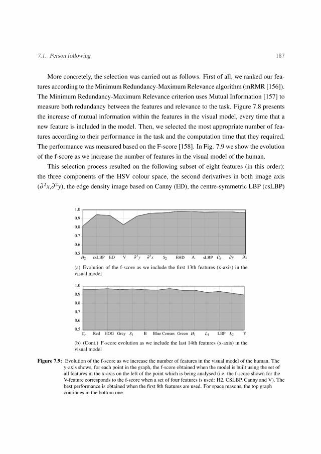
7.1. Person following 187
More concretely, the selection was carried out as follows. First of all, we ranked our fea-tures according to the Minimum Redundancy-Maximum Relevance algorithm (mRMR [156]).The Minimum Redundancy-Maximum Relevance criterion uses Mutual Information [157] tomeasure both redundancy between the features and relevance to the task. Figure 7.8 presentsthe increase of mutual information within the features in the visual model, every time that anew feature is included in the model. Then, we selected the most appropriate number of fea-tures according to their performance in the task and the computation time that they required.The performance was measured based on the F-score [158]. In Fig. 7.9 we show the evolutionof the f-score as we increase the number of features in the visual model of the human.
This selection process resulted on the following subset of eight features (in this order):the three components of the HSV colour space, the second derivatives in both image axis(∂ 2x,∂ 2y), the edge density image based on Canny (ED), the centre-symmetric LBP (csLBP)
(a) Evolution of the f-score as we include the first 13th features (x-axis) in thevisual model
(b) (Cont.) F-score evolution as we include the last 14th features (x-axis) in thevisual model
Figure 7.9: Evolution of the f-score as we increase the number of features in the visual model of the human. They-axis shows, for each point in the graph, the f-score obtained when the model is built using the set ofall features in the x-axis on the left of the point which is being analysed (i.e. the f-score shown for theV-feature corresponds to the f-score when a set of four features is used: H2, CSLBP, Canny and V). Thebest performance is obtained when the first 8th features are used. For space reasons, the top graphcontinues in the bottom one.

188 Chapter 7. Integration with a tour-guide robot
and the edge histogram based on the MPEG-7 edge histogram (EHD). This subset of visualfeatures will be used from now on to identify and distinguish the robot’s target from thedistractors.
Online feature weighting
We have just described how we have selected a suitable set of visual features to distinguishthe robot’s target from the distractors. All of these features describe different properties of animage, and most of the time all of them are useful to discriminate between humans. However,there might be some complex situations in which some features are more discriminant thanothers, or even situations where some features will not allow that discrimination. Since thenumber of possible situations that a robot might encounter when working with humans islarge, we believe that the robot itself must be able to adapt its visual models for each situation.The algorithm that we describe in this section provides our tour-guide robot with the necessaryadaptability to these real world situations.
Starting from the procedure described in Sec. 7.1.2, we replace Eq. 7.3 with a new mea-surement that considers the weights w f of the different features:
Pap(h j|ri) = similarity(h j,ri) =
n f
∑f=1
w f d f (h j,ri) ∈ [0,1] (7.6)
These weights will be updated dynamically according to:
w f ∝ w f + score f (7.7)
where score f measures the ability of each feature to distinguish target from distractors.We must bear in mind that these weights must be normalised. After testing several scorefunctions [147], we have decided to use a score function based on the Bhattacharyya distanceamong histograms (defined in Eq. 7.4). Basically, the best feature should be the one that: a)minimises the Bhattacharyya distance between the feature histogram of the region classified astarget and the target model (d f ,1, in Eq. 7.8), and b) maximises the average distance betweenthe histograms of the distractors and that of the current target model (d f ,2 in Eq. 7.8):
score f = d f ,2−d f ,1 (7.8)
This way, the online feature weighting process adapts dynamically the weight of the visualfeatures that compose the visual model to enhance the discrimination between the target and
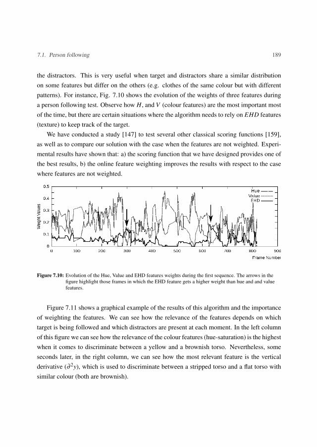
7.1. Person following 189
the distractors. This is very useful when target and distractors share a similar distributionon some features but differ on the others (e.g. clothes of the same colour but with differentpatterns). For instance, Fig. 7.10 shows the evolution of the weights of three features duringa person following test. Observe how H, and V (colour features) are the most important mostof the time, but there are certain situations where the algorithm needs to rely on EHD features(texture) to keep track of the target.
We have conducted a study [147] to test several other classical scoring functions [159],as well as to compare our solution with the case when the features are not weighted. Experi-mental results have shown that: a) the scoring function that we have designed provides one ofthe best results, b) the online feature weighting improves the results with respect to the casewhere features are not weighted.
Figure 7.10: Evolution of the Hue, Value and EHD features weights during the first sequence. The arrows in thefigure highlight those frames in which the EHD feature gets a higher weight than hue and and valuefeatures.
Figure 7.11 shows a graphical example of the results of this algorithm and the importanceof weighting the features. We can see how the relevance of the features depends on whichtarget is being followed and which distractors are present at each moment. In the left columnof this figure we can see how the relevance of the colour features (hue-saturation) is the highestwhen it comes to discriminate between a yellow and a brownish torso. Nevertheless, someseconds later, in the right column, we can see how the most relevant feature is the verticalderivative (∂ 2y), which is used to discriminate between a stripped torso and a flat torso withsimilar colour (both are brownish).

190 Chapter 7. Integration with a tour-guide robot
0
0.1
0.2
0.3
0.4
0.5
0
0.1
0.2
0.3
0.4
0.5
H2 S2V ∂ 2x∂ 2yED EHDcsLBP H2 S2V ∂ 2x∂ 2yED EHDcsLBP
Weighting
Not weighting
Figure 7.11: Two situations where the online feature weighting selects the most appropriate features to discriminatethe target (brownish with horizontal stripes) from the distractor present at each moment. Left column:the distractor’s torso is of a different colour, therefore H2 and S2 are selected. Right column: thedistractor’s torso colour (when mixed with the background) is similar to the target colour, however thehorizontal stripes are a good choice to discriminate amongst both torsos, therefore the weight of ∂ 2y isincreased.

7.2. Human robot-interaction 191
7.1.3 Person following controller
Once the robot is able to detect and track the target, it must follow him around the environ-ment. In this case, the robot’s controller must: a) avoid obstacles and b) maintain the human ata safe distance (e.g. 1 meter), centred in the robot’s field of view. We have designed an ad-hoccontroller based on the potential fields technique [145]: the target position exerts an attractiveforce, and the obstacles around the robot determine the repulsive forces. The target positionis provided by the human tracking module (Sec. 7.1.2), and the repulsive vector by the lasersignature. From the sum of both attractive and repulsive forces we obtain the resultant force,that can be translated into a linear and angular velocity in order to follow the human target.On the other hand, we also want to maintain a safe distance with the human. Therefore, wewill not send linear velocities other than zero to the robot when the distance with the targethas been met.
The main advantage of this method is that it is very simple to implement and fast tocompute, while it gives good results in most situations. However, we have observed somedrawbacks, such as when many people is surrounding the robot. In this case, the repulsiveforces are strong and might modify the robot’s trajectory in a way that makes the robot loseits target. A similar problem arises when the robot is working in narrow spaces or when ittries to cross some doors: either it moves really slow or it is unable to follow the human.
7.2 Human robot-interaction
In the previous section we have described an essential part of the human-robot interaction:how to detect, identify, discriminate and track humans from our robot. In this section, we willdescribe how the robot communicates with the users. We will consider two kinds of users: theroute instructor, and the visitor of an event where the robot operates. The robot’s instructorwill be able to: a) teach new routes to our robot, and b) record voice messages that describepoints of interest within the route. On the other hand, the visitor will have the opportunity toselect a route from those that were taught by the instructor. Then, our robot will follow theroute path, stopping at each point of interest and reproducing the corresponding message.
We can classify the human-robot interaction of our tour-guide robot depending on thedirection of the communication:
– From human to robot (gesture interaction). The instructor will be able to: a) tell therobot that he will be teaching a route, b) tell the robot when to start and stop recording

192 Chapter 7. Integration with a tour-guide robot
a voice message within the route, and c) tell the robot that the route teaching processhas finished. On the other hand, the visitors will be able to: a) ask the robot about theroutes available, and b) ask the robot to show them the desired route.
– From robot to human. Our robot provides information of two different kinds: a) graph-ical user interface with augmented reality and voice feedback (to ease the interactionwith the users), and b) voice messages and sounds while reproducing a route.
The interaction scheme that we have designed [160] for our tour-guide robot is intended tolet everyone use our robot with an very short training period. Our solution consists on: a) thehand interaction (gestures), and b) an augmented reality graphical user interface (AR-GUI)with voice feedback.
7.2.1 Hand gesture recognition
The users of our tour-guide robot will be able to send commands to it using hand movements.To this extent, our robot needs to localise and track the hands and recognise the gestures. Wecurrently recognize the following gestures: wave, push, join hands, and the swipe-left/right
gestures. Whenever the robot recognizes one of these gestures, it carries out the actionsassociated to it.
First of all, when a new user is in front of the robot, the robot will ask him to hold hishands up towards the robot as illustrated in Fig. 7.12. Then, the robot analyses the rangeimages provided by the RGB-D camera in order to look for two hand-sized objects located infront of the user at a certain height. This initialisation was in general accepted by the userswho tested the system, who did not consider it an awkward requirement.
Then, the robot tracks the hands and tries to recognise gestures from the history of posi-tions. To this extent, we model each gesture with a Finite State Machine (FSM) [161]. Thisreduces complexity and overhead, and has proved to perform reasonably well. The inputs ofthe FSM are series of points that describe lines in the 3D space filtered with the least-squaresmethod. A gesture usually comprises between 10 and 30 consecutive points (this marginintroduces speed tolerance and flexibility in the gesture trajectory).
Figure 7.13 shows four trajectory samples and the outcome of each one when it matchesa swipe-left gesture. Examples A and B are accepted as swipe-left gestures showing certaingesture size and speed tolerance. Example C is rejected because although the hand trajectory

7.2. Human robot-interaction 193
Figure 7.12: The robot is detecting a human who stopped in front of it. The human raises his hands up towards therobot. This allows the robot to detect the hands and start tracking them, in order to recognisecommands from the human.
could fit the pattern, it is performed very slowly. Example D is rejected because the handtrajectory does not fit the line.
The tracking and recognition processes run in less than 30ms. Therefore, it is highlyunlikely that we will lose the hands due to rapid hand movements. On the other hand, theseprocesses employ only range data, so we will be able to detect the hands in any environment,regardless of the background colour (there is no interference between it and the hands).

194 Chapter 7. Integration with a tour-guide robot
A
B
C
D
Figure 7.13: Different examples of gesture recognition and rejection for the swipe-left pattern (simplified in the 2Dspace). The gesture start and end points are drawn with green points. The gesture path is representedwith the dotted line and the red points. The black arrow simulates the straight line that fits the points.
7.2.2 Augmented reality graphical user interface with voice feedback
In order to help the user and guide his communication with the robot, we have designedan augmented reality graphical user interface (AR-GUI) with virtual buttons which can beactivated using hand movements. The AR-GUI provides on-screen information and voicefeedback to keep the user informed about what the robot is sensing and what he expects fromthe user at every moment. The AR-GUI is the users’ window to what the robot sees, thinks,and expects from him.
The AR-GUI is the central element of our robot’s interaction capabilities. It is displayedin the robot’s screen, and its main characteristic is that the user can see himself as in a mirror,along with several virtual elements which ease the interaction. Currently, the virtual elementsthat we use are (see Fig. 7.14):

7.2. Human robot-interaction 195
A B C
D E F
G H I
J K L
Figure 7.14: Augmented reality graphical user interface (AR-GUI) displayed on the robot’s screen. We can see howa user enters the robot’s field of view, initialises his hand positions and starts giving commands to therobot.

196 Chapter 7. Integration with a tour-guide robot
– The human body is shaded with a random colour when he is being detected by the robot.Moreover, in case that a human is the robot’s target (i.e. when following him), his bodyis shaded in green.
– When a human is performing the initialisation pose to let the robot detect his hands(Fig. 7.12), two red boxes will pop up, to indicate where the user should put his hands.
– Blackout of the areas not visible for the robot: i.e. if a human is outside the workingrange of the robot’s human detector, he will not appear in the screen.
– Two virtual balls, drawn over each hand while they are being detected and tracked.
– Virtual buttons to command actions to the robot: i.e. the instructor of our robot will beable to start recording a new route by holding his hand over a virtual button for a coupleof seconds.
In Fig. 7.14 we can see a sequence of screenshots from the AR-GUI taken when perform-ing a typical interaction with our guide robot. First, when a human walks into the robot’s fieldof view (Fig. 7.14.A), his body is coloured in a random colour distinct from green. Then,when that user is standing in front of the robot a voice message asks him to please, put your
hands up towards the robot, and immediately two red boxes are drawn at the positions wherethe user should put his hands (Fig. 7.14.B). This step helps a robot’s user to correctly performthe initialisation pose.
When the robot has detected the user’s hands, the hand positions are marked with twovirtual balls. At the same time, two buttons (one for recording and another for reproducingroutes), appear on the screen (Fig. 7.14.C), and a voice message requests the user to select anaction. Then, the user of our example can activate the record a new route button by holdinghis hand over it for a couple of seconds, as shown in Fig. 7.14.D. At that point, the AR-GUI shades his body in green (Fig. 7.14.E) and the robot starts following the user around theenvironment. Again, the user receives information via voice about the action: the robot is nowrecording a route. At any point, the user may record a voice message by activating the buttonto record a voice message (Fig. 7.14.F), speaking loudly to the robot, and then stopping therecording by pressing a button again. The message will be reproduced immediately afterwardsto offer the user a chance to record it again. The voice message will be stored with the routeinformation, and can thus be reproduced at the same point of the route where it was recorded.Once the user has taught the new route to the robot, he activates the stop the route recording

7.3. The route recording and reproduction architecture 197
button (Fig. 7.14.G), and the information on the route is stored in the robot, so that the robotcan reproduce it afterwards.
Once the robot has learnt several routes, it can offer its guidance services to anyone whostops in front of it, and asks for a route to be reproduced by activating the button as shownin Fig. 7.14.H. This button leads to a sub-menu with as many buttons as routes are available(Fig. 7.14.I), while the robot reproduces a voice message asking to choose one route. Whenthe user choses a route, the robot finishes the hand interaction (Fig. 7.14.J) and starts reproduc-ing this route. Finally, when a user decides that he no longer wishes to interact with the robot,he can wave off. A voice message saying goodbye is reproduced and his body will appearshaded in a colour other than green. This process is shown in Fig. 7.14.K and Fig. 7.14.L.
It is important to note that our guide robot allows humans to walk freely. In the case thatthe user is walking too fast for the robot, he is informed by a voice message to please, walk
slower. Also, if the user walks outside the working range, he is informed with a voice messagesaying, I lost you, and then the user is responsible for coming back to be recognised by thesystem.
7.3 The route recording and reproduction architecture
In this section, we will describe the architecture that allows our robot to learn routes from aninstructor and to reproduce them in front of users.
7.3.1 Route recording architecture
Figure 7.15 illustrates the route recording process, as well as the rest of the elements involvedin the process (the localisation algorithm, the AR-GUI, and the voice recording process), andthe communication between all of them. We have integrated our system using ROS (RobotOperating System). The localisation algorithm is an asynchronously, always-working, inde-pendent node. That is, it is continuously estimating the robot’s pose with every new sensorinformation available. During the entire recording, the pose estimation should be correct andprecise (errors below 1 meter). This is one of the reasons why we have made an special effortinto obtaining a robust localization solution. On the other hand, the route recording processmay be launched by the instructor at any time. Then, it remains in the background, waking upin two cases:

198 Chapter 7. Integration with a tour-guide robot
Figure 7.15: Schematic representation of the route recording process of our tour-guide robot, as well as the rest ofthe elements that take part in this process.
– When the localisation algorithm estimates a new pose (~st ). In this case, it will decidewhether to store ~st or not based on how far ~st is from the latest pose stored in the route.
– When the AR-GUI informs about a point of interest. In this case, it will store the voicemessage recorded by the instructor, alongside the latest estimated robot pose (~st ).

7.3. The route recording and reproduction architecture 199
Therefore, the routes of our robot are composed of a sequence of robot poses (which wecall way-points), intercalated with point of interest (which consist of a robot’s pose and avoice message). This data will be used by the route reproduction process to mimic the path ofthe robot and to reproduce the voice messages at the same places where they were originallyrecorded.
7.3.2 Route reproduction architecture
A visitor of an event can demand any route from our tour-guide robot, regardless of the placewhere the robot is. This means that the first task that our robot has to accomplish is to travel tothe first point of the route from its current position. Then, it will need to reproduce the routein the most accurately, dealing with the dynamic nature of the environment.
In order to describe this process, we can define a route r as a list of robot’s poses ~sr1, ...,
~srnr where nr is the number of stored poses (or way points). Some of these way points can
actually be points of interest, if they are associated with voice messages. The goal of the routereproduction behaviour of our robot is to visit each of those points in the specified order, andto reproduce the associated voice message if there is one.
Global planner: navfn
In Fig. 7.16 we can see that the route reproduction process starts when the AR-GUI demandsa route (start route). At this moment, the behaviour picks a way point (~sr
1) and plans a validpath from the robot’s pose (~st ) to that point. These points can be separated several dozenof meters, and planning a valid path might not be a trivial problem. In our case, we havechosen a classical solution, Dijkstra’s algorithm [162]. It is a good solution in terms of effi-ciency and simplicity, and it was able to provide good results in all cases that we have tested.More specifically, we have used an improved version which is available in the ROS globalnavigation planner navfn 1.
This algorithm requires us to build a cost-map of the environment where the robot operates(global costmap in Fig. 7.16). This costmap will be used as the graph in which Dijkstra’salgorithm will search for a minimum cost plan between the two points. In order to build thecostmap of the environment we need: a) an occupancy map of the environment (which iscreated during the deployment stage of the robot, as described in Sec. 5.5), b) the robot’s
1http://wiki.ros.org/navfn

200 Chapter 7. Integration with a tour-guide robot
Figure 7.16: Schematic representation of the navigation node used for route reproduction in our tour-guide robot. Itis a ROS based node with a global planner for path planning (navfn) and a local planner based on theDynamic Window Approach (DWA) for navigation.
estimated pose ~st , c) the current data from the laser scanner, and d) the radius of the robotminr.
The costmap is initialised using the occupancy map of the environment: we assign thehighest value in the costmap to those cells that are marked as occupied in the occupancy map,and a low value to those cells that are marked as free space. Then, using the robot’s estimatedpose and the laser signature, we create new occupied cells in the costmap, and in the same way,we also release cells that were previously marked as occupied. We need to do this becausethere might be obstacles in the environment that are not in the map, such as humans, but there

7.3. The route recording and reproduction architecture 201
might also be furniture which has been moved, releasing previously occupied space. The laststage to build the costmap consists in marking as occupied those free cells that are closer thanminr to an occupied cell, as the robot will not be able to visit those cells without colliding.This process is known as inflating the obstacles of the map.
Local planner: Dynamic Window Approach
At this point, our algorithm will use the costmap to plan a valid path from the robot’s positiontowards the start point of the route. This plan will be handed out to a second element: thelocal navigation planner (Fig. 7.16). The local planner is the element responsible for movingsafely our robot in the environment, while it follows the path plan. In order to face thisproblem, we use a popular algorithm that is able to solve the task with an small computationaloverhead: the Dynamic Window Approach (DWA) 2 [163]. Basically, this algorithm simulatesvarious trajectories which are generated by sampling the linear and angular velocities of therobot. Then, each simulated trajectory is scored according to different criteria. In the end, thetrajectory with the highest score is chosen, and the velocities which generated that trajectoryare executed in the robot’s base. This algorithm allows us to continuously re-evaluate therobot’s trajectory, and thus avoid dynamic obstacles such as persons walking in the robot’spath.
An important element of DWA is how we score the simulated trajectories. In each cycle,we need to create a second costmap, which we call the local costmap. In order to do this, weuse the laser signature and the computed path plan. First, obstacles are inflated in the sameway than in the other costmap, and then we assign different weights to the free space cells,according to how far they are from the planned path. Therefore, using this local costmap,trajectories can be scored taking into account how close they are to the desired path and ondifferent parameters like proximity to obstacles or achieved speed.
Route execution
When our tour-guide robot has reached the start point of the route, it will make a short beep(Reproduce sound in Fig. 7.16), pick the next way point and start a similar process to navigatetowards it. That is, we will compute a new path plan using Dijkstra’s algorithm and safely
2http://wiki.ros.org/dwa_local_planner

202 Chapter 7. Integration with a tour-guide robot
execute it using the Dynamic Window Approach. We repeat this process until the last pointof the route is reached or the visitor stops the robot.
Additionally, our route might contain points of interest, which are treated similarly to anormal way-point. The main difference is that the robot will stop in that point for a while,until the associated voice message is fully played back (Reproduce sound in Fig. 7.16).
Finally, we have also implemented several rules to increase the flexibility of the robot,and to deal with unreachable route points. First, we consider a point as visited when the robotmoves at a close distance (0.5m from the route point). This prevents our robot from spendingmany seconds moving slowly to reach a goal pose with a high precision, and thus increasesthe overall robot’s speed. Second, when our robot’s detect that a point within the route isunreachable, i.e. a human is blocking the path, we proceed in two different ways. In the firstone, the robot will clear his local costmap from the nearest obstacles and perform an in-placerotation to check for alternative paths. If there is still no valid path, the robot will perform amore aggressive reset of the costmap, completely clearing it and performing another in-placerotation to rebuild it. If this also fails, we will consider the second alternative: the robot iscompletely blocked, and therefore we will allow it to skip that way-point and move to thenext one. In case that the robot skips a point, it will make a recognisable error sound to let theuser’s know that there was a problem.
7.4 Tests in the robotics laboratory
In this section, we want to illustrate the performance of the route reproduction module thatwe have designed for our tour-guide robot. For this reason, we will describe two routes thatwe have recorded in our robotics laboratory (Fig. 7.17). In this laboratory we have settled anindoor environment with five rooms. We have chosen this laboratory as the first test-bed forthe route-management in our robot because it is similar in size (100m2) and space arrangement(five rooms) with most homes or offices nowadays.
The routes that we have recorded are illustrated in Fig. 7.18 with a dotted line (robot’strajectory during recording) and small dark grey circles (recorded way-points). The resultobtained when reproducing the route is illustrated in Fig. 7.18 with a light grey line. In theseexamples we can see how the robot has to previously find a valid path from its initial pose (Cin Fig. 7.18) to the initial point of the route (A in Fig. 7.18). Once the robot has reached thefirst point of the route, it moves from one way-point to the next one, avoiding obstacles in the

7.4. Tests in the robotics laboratory 203
environment (two humans walking randomly) without separating from the path more than afew dozens of centimetres. Moreover, when the robot reached a point of interest, it played thevoice message recorded by the instructor. Finally, when the robot finished the reproduction ofthe route, it played a bell sound and waited for new commands from any other human.
The first route (Fig. 7.18, left) was recorded in 56 seconds, and it is 15.3 m long. In thisroute no points of interest were recorded by the instructor, but it is interesting in order tonotice how fast can anyone teach a route path to the robot in a home-like environment withnarrow corridors. In this experiment, the robot had to travel 29.2 m in order to find the firstpoint of the route and mimic the complete route path.
The second route (Fig. 7.18, right) was recorded in 155 seconds, and it is 40.8 m long.When reproducing this route the robot travelled 52.8 m. In this route, the instructor recordedthree voice messages at the points of interest. These messages were very short: around 5seconds each one. Our tour-guide robot allows the record and reproduction of a complexroute in few time by non experts.
Moreover, we have showcased our tour-guide robot during many demonstrations in ourresearch centre (CITIUS). These demonstrations are part of a program for visitors, in whichwe show them the results of our research activity. In this regard, Fig. 7.19 shows a pictureof a visitor teaching our robot a route inside our laboratory (Fig. 7.17). Then, the rest of the
Figure 7.17: CITIUS robotics laboratory (100m2) where we have conducted several route reproduction tests. We setup an environment with 5 rooms, and recorded and reproduced several routes while two humans werewalking around.

204 Chapter 7. Integration with a tour-guide robot
Figure 7.18: Robot trajectories while recording (dotted) and reproducing (light grey) two routes. The small circlesrepresent the stored way-points. The points marked with the letters A and B represent the first and lastpoints of each route, respectively. The points marked with letter C are the location of the robot when itwas asked to reproduce the route, and the points marked with the letter D in the second route are thelocations of points of interest as specified by the route teacher.
pictures show how our robot reproduces a route that it has just learnt. In many demonstrationsour tour-guide robot did not have problems to reproduce the routes, however in some of themit had to perform in-place rotations to clear out blocked space. This situation happens whenthe environment differs significantly from the one in the occupancy map of the robot, whichmight be a common problem when the visitors are mainly kids who play around with furniturein our laboratory.
7.5 Discussion
In this thesis, we have integrated our intelligent space with a general purpose guide robot thatwe have developed in the past, as an specific example of application. This robot is aimed tooperate in different environments, such as museums, conferences, or robotics demonstrationsin research centres. Our robot is able to detect and track people around him, follow an instruc-tor around the environment, learn routes of interest from the instructor, and reproduce themfor the visitors of the event. Moreover, the robot is able to interact with humans using gesturerecognition techniques and an augmented reality interface.
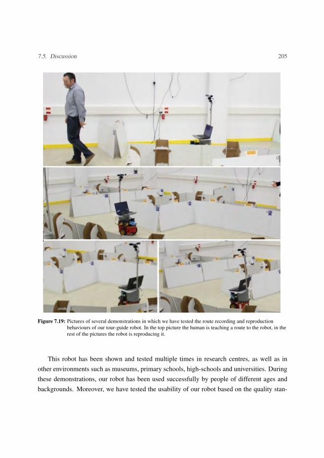
7.5. Discussion 205
Figure 7.19: Pictures of several demonstrations in which we have tested the route recording and reproductionbehaviours of our tour-guide robot. In the top picture the human is teaching a route to the robot, in therest of the pictures the robot is reproducing it.
This robot has been shown and tested multiple times in research centres, as well as inother environments such as museums, primary schools, high-schools and universities. Duringthese demonstrations, our robot has been used successfully by people of different ages andbackgrounds. Moreover, we have tested the usability of our robot based on the quality stan-

206 Chapter 7. Integration with a tour-guide robot
dard ISO/IEC-9126-4, by monitoring the users while they interacted with our robot and bygathering their opinions through polls.

CHAPTER 8
SITUM: INDOOR POSITIONING FOR
SMARTPHONES
We believe that we, as researchers, have the responsibility to transfer the knowledge thatwe create to society. This means, of course, to publish articles, to educate students, to fillpatents and to participate in divulgative activities. In addition, we believe that one of ourmain responsibilities is to actually apply the technologies we create to solve the problems ofsociety, to create commercial value.
For this reason, in 2013 we started studying the possibility of creating an indoor position-ing technology for smartphones. Nowadays, this germinal idea has given birth to a companycalled Situm Technologies, a spin-off of the University of Santiago de Compostela. Situm hasgrown up to a team of 11 members and is already selling its products and generating revenue.
In this chapter, we will provide a brief description of Situm: its initial idea, its technologyand products, its business model, its team, its achievements and its future.
8.1 The problem, the idea, and the first contact with the market
Every product must solve a real problem or need for real people. This is a basic and fun-damental law when the goal is to launch a product into the market. No matter how unique,technologically advanced, elegant, disruptive and well designed the product is, if it does notsolve a real problem for which customers are willing to pay, it is worthless.

208 Chapter 8. Situm: indoor positioning for smartphones
In our case, the problem was that the GPS does not work indoors. We knew that theGPS had enabled the proliferation of Location Based Services (LBS), such as guidance fordrivers and pedestrians, but these services could only be used outdoors. If we had a reliableindoor location technology (a GPS for indoor spaces), a new world of services would bepossible. The market growth estimations agreed with this perspective. In fact, the globalindoor location market was estimated to be $935.05 million in 2014 and expected to growto $4,424.1 million by 2019. This represents an estimated Compound Annual Growth Rate(CAGR) of 36.5% from 2014 to 2019 (source: MarketsAndMarkets1). This told us two things:1) that the indoor positioning problem was relevant for a big number of potential customers,and 2) that customers were willing to pay for solutions related to this problem.
Under this perspective, we identified a number of sectors where indoor positioning tech-nologies could be applied: shopping malls and commercial areas, supermarkets, museums,hospitals, airports, etc. We envisioned a number of use cases for each sector. With an ade-quate solution, passengers on airports could get step-by-step guidance to their boarding gates,hospitals and factories could know the position of their employees to respond faster on emer-gency situations, commercial centres and supermarkets could know the position and trajectoryof each costumer and obtain relevant information for marketing studies, etc. Then, we iden-tified local people involved in each sector, and met with some of them to present them ourideas. Our objective was to gather information about the different applications of an indoorpositioning technology in each sector, and to propose the development of pilot projects to testthe use cases. The feedback from the first meetings was very positive, so we decided to builda prototype of an indoor positioning technology.
8.2 The technology
In 2013, indoor positioning companies (e.g. Ekahau) were offering technologies that requiredthe installation of expensive hardware and/or could only track the position of specific hard-ware devices (e.g. hardware tags). These technologies could only be applied to domainswhere it was be possible to afford the installation costs and where the users would agree oncarrying the tracking devices (e.g. hospitals or industrial plants). Moreover, from our experi-ence with Ekahau, an state of the art system, we knew that these technologies could not offerenough precision and robustness for demanding applications, such as turn-by-turn guidance.
1http://www.marketsandmarkets.com/PressReleases/indoor-location.asp

8.2. The technology 209
We believed that an indoor positioning technology that aspired to reach the mass marketshould be compatible with modern smartphones, because their adoption was on track to be-come universal. Therefore, we developed our own indoor positioning technology for thesedevices. This technology is based on:
1. Intelligent sensor fusion. Our technology is able to fuse the information received fromthe different sensors of the smartphone: WiFi, Bluetooth Low Energy (BLE) and mag-netometer. This makes our technology robust and versatile.
2. Inertial navigation. To achieve the highest precision, our technology estimates the dis-placement of the user from the readings of the accelerometer and gyroscope of thesmartphone.
3. Cloud computation. A server receives the sensor information from every smartphone,estimates its position and sends it back (Fig. 8.1).
The results were very positive. First of all, our technology could achieve high precision(up to 1 meter) and robustness. Second, it could be configured very quickly in any building,mainly because it could work with existing WiFi networks without installing additional hard-ware. Finally, unlike most competitors, our technology could work in multi-level buildings.
Figure 8.1: Cloud-based indoor positioning technology.

210 Chapter 8. Situm: indoor positioning for smartphones
This technology, by itself, did not solve any problem for which a customer was willing topay. Therefore, we created a product that used this technology, and that could provide valueto potential customers.
8.3 The product
On top of our indoor positioning technology, we built a Software Development Kit (SDK),illustrated in Fig. 8.2. The idea was to enable any developer to build apps and location basedservices based on our technology. Other than the cloud-based positioning server, the SDKconsists on two components:
1. Situm Dashboard. Web panel that allows to configure our indoor positioning system:create a new building and upload its map, create points of interest to where users can beguided (e.g. emergency exits), create alerts that users will receive when passing througha certain area (e.g. shopping promotions), etc. In addition, this panel shows positioningstatistics: number of visitors within a period, popularity of each area of the building,etc.
Figure 8.2: Situm Software Development Kit.

8.4. The business model 211
2. Situm API. Set of tools oriented to the development of apps for Android/iOS. Thesetools allow any developer to integrate our technology into any smartphone app, in a fastand easy manner.
In paralell, we worked on the definition of a business model that would allow us to sellthis product to our customers.
8.4 The business model
Currently, we offer our products to software development companies that want to create lo-cation based apps for their clients. The revenue model is based on license fees and royaltieson the final product revenues. In addition, in some sectors we are exploring the possibility ofdeveloping final products ourselves.
8.5 The team
Situm has 11 team members at the moment. All the founders are or have been researchersof the CITIUS: Dr. Victor Alvarez-Santos (Chief Executive Officer), Adrian Canedo (ChiefTechnology Officer) and Dr. Cristina Gamallo (R&D manager). Each of them has worked forseveral years in the topics of indoor positioning and robotics. They have more than 25 sci-entific publications, a wide experience in software development, and business training. Thedevelopment team is completed by 6 developers with a wide experience on their respective ar-eas: Felix Queiruga (web back-end), Maria Reino (web front-end), Pablo Vazquez (web front-end), Abraham Barros (mobile), Javier Casanova (mobile), and Dario Villar (C++). Finally,Miguel Perez is in charge of corporate communication, and Daniel Sanmartin of finance.
The company also counts with the invaluable support of the other three founders, that playthe role of scientific advisors on the topics of indoor positioning and machine learning: Dr.Senén Barro and Dr. Roberto Iglesias (University of Santiago de Compostela, Spain) and Dr.Carlos V. Regueiro (University of A Coruña, Spain).
8.6 Achievements
Situm has already developed the core of the indoor positioning technology and product. Ithas installed the technology in 9 buildings: 4 in Santiago de Compostela, 4 in Madrid and 1

212 Chapter 8. Situm: indoor positioning for smartphones
in Barcelona. It has also several projects going on with clients of different sectors, the mostimportant as a technology provider of Telefónica. In this project, it will install the indoorpositioning system in 22 Galician hospitals and health centers.
In addition, Situm has received several recognitions:
1. Winners of the Smart Ideas contest 2014 (Smart City program, Council of A Coruña).
2. First national price in Yuzz 2014 (Banco Santander, CISE).
3. First price in Galicia Open Future 2015 (Xunta de Galicia, Telefónica).
4. Best elevator pitch at the Singularity University events (supported by entities such asNASA, Google and the IMPACT accelerator).
Finally, Situm has been backed financially by S. C. R. Unirisco (venture capital) andENISA.
8.7 Future
Situm started 2 years ago as a compromise between 3 PhD students and 3 senior researchers,that wanted to apply their know-how to build a product that could enter the market. Nowa-days, Situm has a team of 11 members that has developed a tangible product that is alreadygenerating revenue (more than 100.000 AC so far). In the future, Situm aspires to maintain atechnologically advanced product able to evolve according to the requirements yet to come,and to provide its technology in buildings all around the world.

CHAPTER 9
CONCLUSIONS
The goal of this thesis was to develop robotic systems that are able to operate robustly indynamic and non structured environments. In addition, we wanted to be able to deploy thesesystems in different environments in a fast and easy manner, and to provide robots with ini-tiative to respond proactively to the needs of the users. To this extent, we have combinedtechnologies from ubiquitous computing, ambient intelligence, and robotics. More specifi-cally, we have built an intelligent space that consists of a distributed network of intelligentcameras and autonomous robots. The cameras are spread out on the environment, detectingsituations that might require the presence of the robots (call events), informing them aboutthese situations, and also supporting their movement in the environment. The robots, on theother hand, must navigate safely within this space towards the areas where these situationshappen. With this proposal, our robots are not only able to react to events that occur in theirsurroundings, but to events that occur anywhere. As a consequence, the robots can react to theneeds of the users regardless of where the users are. This will look as if our robots are moreintelligent, useful, and have more initiative. In addition, the network of cameras will supportthe robots on their tasks, and enrich their environment models. This will result on a faster,easier and more robust robot deployment and operation. The intelligence needed to achievea robust performance of the system can be distributed amongst all the agents, cameras androbots in our case. In this thesis, we have explored two alternatives: collective intelligenceand centralised intelligence.
Under the collective intelligence paradigm, intelligence is fairly distributed among agents.Global intelligence arises from individual interactions without the intervention of a central

214 Chapter 9. Conclusions
agent, similarly to self-organization processes that occur in nature. We have assumed thatrobots can operate in a priori unknown environments when their behaviour emerges from theinteraction amongst an ensemble of independent agents (cameras), that any user can placein different locations of the environment. These agents, initially identical, observe humanand robot behaviour, learn in parallel, adapt and specialise in the control of the robots. Tothis extent, our cameras were able to detect and track robots and humans robustly, underchallenging conditions: changing illumination, crowded environments, etc. Moreover, theycould discover their camera neighbours, and guide the robot navigation through routes ofthese cameras. Meanwhile, the robots only had to follow the instructions of the cameras andnegotiate obstacles in order to avoid collisions. In order to accomplish this, we have achievedthe following milestones:
1. We have designed and implemented a network of cameras that can be deployed in afast and easy manner in different environments. Our cameras have high computationcapabilities and can work connected to a wall plug or using their own batteries with anautonomy of up to 4 hours. Moreover, they can communicate wirelessly among themand with the robots.
2. We have developed a software architecture that controls the interaction amongst allthe agents of the system. This architecture considers the existence of two differentagents: robot-agents and camera-agents. The architecture is fully distributed and veryscalable. This allows us to remove or introduce agents in the system with minimumreconfiguration requirements.
3. We have studied the possibility of detecting and tracking the robot from the camerasusing object recognition techniques and techniques based on the detection of passivemarkers mounted on the robot (markers that do not emit light). However, none ofthese techniques has given satisfactory results in the context of application of this the-sis. Therefore, we have designed and developed an algorithm for robot detection andtracking based on active markers. Our algorithm has shown to be very robust in realexperiments, and can work in real-time. Moreover, we have shown that we can de-tect and track multiple robots, and even identify each of them, while the computationalrequirements scale linearly with the number of robots.
4. We have developed a system to detect situations that may require the presence of therobots from the cameras. Specifically, we have developed algorithms for the detection

215
of: 1) people waving at the cameras, 2) people standing in certain areas. Both algo-rithms have been proposed as specific examples of call events that might require thepresence of our robots. We would like to point out that the concept of call event can beaccommodated to a wide range of robotics applications. For instance, we could detectwater spills to aid a cleaning robot, potential threats to aid a security robot, etc. More-over, call events could be triggered by other kind of devices: for instance, the user coulduse a “tag” or an smartphone to call the robot.
5. We have developed a set of algorithms that allows the system to work under the collec-tive intelligence paradigm. With these algorithms, the cameras where able to: 1) detecttheir camera neighbours, 2) construct routes of cameras through which the robot cannavigate, 3) assign a call event to an available robot, 4) support the robot navigationtowards this call event. We have shown that our cameras can establish neighbourhoodlinks when their Fields of View (FOVs) overlap, attending at simultaneous detections ofthe robot. In other case: 1) the robot can construct maps for navigation between neigh-bour cameras (e.g. occupancy maps from a 2D laser scanner), 2) the cameras can detecttheir neighbourhood relationships by re-identifying people walking around. Real worldexperiments have shown the feasibility of our proposal to work with “naive” robots.
On the other hand, under the centralised intelligence paradigm, one type of agent is as-signed much more intelligence than the rest. In this case, the network of cameras will bestill responsible of detecting the call events, and they will support the movement of the robotsin the environment. In particular, they will inform the robot when they see it. Neverthe-less, the robot will be the agent that makes most decision making, and its performance willhave the highest importance. This option implies that the robot is able to estimate its po-sition accurately and robustly, therefore most of the intelligence was devoted to the task ofself-localisation and navigation. Our robots implemented multi-sensor localisation strategiesthat fuse the information of complementary sources, in order to achieve a robust robot be-haviour in dynamic and unstructured environments. Under this paradigm, we have achievedthe following milestones:
1. We have performed an experimental study about the strengths and weaknesses of dif-ferent information sources to be used for the task of robot localisation: a 2D laser rangefinder, a magnetic compass, a commercial WiFi localisation system, and the networkof external cameras. The study shown that no source performs well in every situation,

216 Chapter 9. Conclusions
but the combination of complementary sensors may lead to more robust localisationalgorithms.
2. We have developed a robot localisation algorithm that combines the information frommultiple sensors. This algorithm is able to provide robust and precise localisation esti-mates even in situations where single-sensor localization techniques usually fail. It canfuse the information of an arbitrary number of sensors, even if they are not synchro-nised, work at different data rates, or if some of them stop working. We have tried thisalgorithm with the following sensors: a 2D laser range finder, a magnetic compass, aWiFi reception card, a radio reception card (433 MHz band), the network of externalcameras, and a camera mounted in the robot.
3. We have tested our positioning algorithm with multiple sensors, and we have proposedobservation models for each of them:
a) 2D laser scanner: we have proposed a model that takes into account the differencesamong the expected and received laser signature, both regarding their shape aswell as their concrete values.
b) Compass: we have proposed a model that takes into account the magnetic dis-tortions of the environment, in order to minimise their influence in orientationreadings.
c) WiFi reception card and radio reception card (433MHz band): we have proposedand analysed three different techniques that allowed us to perform indoor posi-tioning based on the power of the wireless signals received.
d) Camera network: we have proposed a model able to estimate the position of therobot based on the list of cameras that detect it at every instant.
e) Camera mounted in the robot: we have developed a model based on scene recog-nition that allows us to estimate the most probable robot position based on animage captured by the camera mounted on the robot.
4. We have performed a complete experimental study of the localisation algorithm, in bothcontrolled and real conditions during robotics demonstrations in front of users. We havestudied the behaviour of the algorithm when using each single sensor and most of theircombinations. Our main conclusion was that, with statistical significance, the fusion of

217
complementary sensors tends to increase the precision and robustness of the localisationestimates.
5. We have designed wireless transmitters (motes) and we have integrated them into ourindoor positioning algorithm. Our motes use an inexpensive, low-power sub-1-GHzsystem-on-chip (CC1110) working in the 433-MHz ISM band.
6. We have studied the performance of our positioning algorithm when the wireless trans-mitters in the environment are able to vary their transmission power. Through an exper-imental study, we have demonstrated that this ability tends to improve the performanceof a wireless positioning system. This opens the door for future improvements in theline of active localisation. Under this paradigm, the robot would be able to modifythe transmission power of the transmitters in order to discard localisation hypothesesproactively.
7. We have integrated our intelligent space with a general purpose guide robot, as an spe-cific example of application. Our tour guide robot is aimed to operate in different socialenvironments, such as museums, conferences, or robotics demonstrations in researchcentres. Our robot is able to detect and track people around him, follow an instructoraround the environment, learn routes of interest from the instructor, and reproduce themfor the visitors of the event. Moreover, the robot is able to interact with humans usinggesture recognition techniques and an augmented reality interface.
8. Finally, we have designed a methodology that allows any user to deploy and calibratethis system in a short period of time in different environments.
The architectures, behaviours and algorithms that have been proposed within this thesiscan go beyond the scope of robotics. In the coming years, robots are called to populatenew environments like hospitals, museums, or offices. These new generations of robots willneed to be able to navigate autonomously and perform robustly under difficult conditions:challenging illumination, people walking around the robot, etc. Moreover, robots will needto be aware of humans regardless of where they are, interact with them, follow them, andcooperate with them. Even more, there is a current trend (“Internet of Things”) to populateour environments with networked devices with processing and sensing capabilities, such ascameras, Bluetooth beacons, and all sorts of sensors. The robotics community should notmiss the opportunity of enriching and improve the robots’ behaviours and services with the

218 Chapter 9. Conclusions
possibility that this new trend offers. For all these reasons, we believe that what has beenproposed within this thesis (in part or as a whole) can be the basis for future robot architecturesand behaviours that might even reach the market in the coming years.
Finally, we would like to highlight that the indoor positioning knowledge derived from thisthesis is the base of Situm Technologies, a company that provides indoor positioning technolo-gies for smartphones. This company has received several recognitions, financial backing froma venture capital fund, and has already generated more than 100.000 AC in revenue.
9.1 Future work
A thesis is not a closed work, but it should open lines of work that may lead to interestingresults in the future. In this regard, we believe that this thesis leaves room for future improve-ment and for new interesting research lines. Just to mention but a few:
1. We have explored two different solutions: collective intelligence and centralised intelli-gence. We demonstrated that it was possible to obtain robust navigation of robots underthe collective intelligence paradigm, by supporting them with a network of intelligentcameras. We have seen as well that this could lead to poor performance if the camerasfailed. As an alternative, we moved most of the intelligence to the robot, leading to arobot that was able to localise themselves and navigate autonomously. This approachhad a problem too: the whole system depended on the construction of a previous mapof the environment, so if the map could not be built for any reason, the robot would fail.We believe that it would be worth to explore an intermediate solution. The camerascould help the robot during the deployment stage, in order to explore the environmentautonomously and calibrate all the systems. Then, the robot could rely on its localisa-tion estimates, unless the localisation algorithm failed, in which case the cameras wouldstill be able to support its navigation.
2. We would like to continue exploring the detection of call events. The Computer Visioncommunity has developed dozens of algorithms aimed at the characterisation of peoplebehaviour. This could be used as a way to infer whether or not the assistance of therobot is needed.
3. We believe that the introduction of smartphones in this system would be very interest-ing. Smartphones have perception and processing capabilities, and they can interact

9.1. Future work 219
with the user. Moreover, as we have demonstrated with our experience at Situm Tech-nologies, they can be localised within the environment with sufficient precision. There-fore, users could use them to call a robot, and the system could track them to infer thebehaviour of the users and trigger call events.
4. We would like to improve the observation models of the external cameras and the cam-era mounted on top of the robot. Both showed good results, but we think that theinformation that they provide has much more potential. For instance, in our currentproposal, when a camera sees the robot, the robot only knows that it is within the FOVof the camera. However, cameras could be used to give a more precise estimation ofthe position of the robot in the map.
5. We would like to explore the use of other sensors in our localisation system. Partic-ularly, we would like to include an omni-directional camera pointing to the ceiling.Gamallo et al. [68] demonstrated that this sensor could be used to obtain very robustglobal and local localisation estimates.
6. We have seen that 3D perception could help our robot in order to avoid dangeroussituations (e.g. falling down stairs) and to achieve a more robust and safe navigation.In addition, it would also be interesting to integrate 3D perception in the positioningprocess.
7. We have seen that the use of varying transmission powers improves significantly theperformance of wireless positioning systems. We will continue on exploring the use ofdifferent power transmission patterns. In addition, we will explore active localisationstrategies, where the robot can modify the power of the transmitters proactively, inorder to discard localisation hypotheses. This opens the possibility of robot-agentsinfluencing the behaviour of other agents of the intelligent environment in order toimprove its own behaviour and being more effective.
8. We would like to explore the use of radio technologies in the 433 MHz band for com-munications amongst the elements of our system.
9. Finally, we will continue on improving our tour-guide robot. Particularly, we wouldlike to: 1) improve the human detector so that it is able to segment humans that aretouching each other, 2) provide a more robust and natural hand-tracking (now it requires

220 Chapter 9. Conclusions
initialisation), 3) enable the robot to learn gestures and associate them with actions, 4)introduce speech recognition techniques.

CHAPTER 10
DERIVED WORKS
This thesis has generated several results of great relevancy. First of all, the contents of thisthesis have been reported in 7 publications in journals indexed in JCR, in 1 publication in ajournal with other quality index, in 6 publications in international congresses and in 4 publi-cations in national congresses. We have also registered our multi-sensor indoor positioningsoftware at the “Oficina Española de Patentes y Marcas” (Spanish Patent and Trademark Of-fice) and we have created the company Situm Technologies, an spin-off of the University ofSantiago de Compostela.
10.1 Publications in journals indexed in JCR
1. A. Canedo-Rodriguez, J. M. Rodriguez, V. Alvarez-Santos, R. Iglesias and C. V.Regueiro. “Mobile Robot Positioning with 433-MHz Wireless Motes with VaryingTransmission Powers and a Particle Filter”. Sensors, vol. 15, pp. 10194–10220, 2015.Impact factor: 2.048 (10 of 57 - Q1 in category: Instruments & instrumentation).
2. A. Canedo-Rodriguez, V. Alvarez-Santos, C.V. Regueiro, R. Iglesias, S. Barro and J.Presedo. “Particle filter robot localisation through robust fusion of laser, WiFi, com-pass, and a network of external cameras”. Information Fusion, available online. Impactfactor: 3.472 (12 of 121 - Q1 in category: Computer Science, Artificial Intelligence).
3. V. Alvarez-Santos, A. Canedo-Rodriguez, R. Iglesias, X.M. Pardo, C.V. Regueiroand M. Fernandez-Delgado. “Route learning and reproduction in a tour-guide robot”.

222 Chapter 10. Derived works
Robotics and Autonomous Systems, vol. 63, p. 2, pp. 206-213, 2015. Impact factor:1.105 (11 of 21 - Q3 in category: Robotics).
4. V. Alvarez-Santos, R. Iglesias, X.M. Pardo, C.V. Regueiro and A. Canedo-Rodriguez.“Gesture-based interaction with voice feedback for a tour-guide robot”. Journal of Vi-
sual Communication and Image Representation, no. 2, vol 13, pp. 499–509, 2014.Impact factor: 1.361 (30 of 105 - Q2 in category: Computer Science, Software Engi-neering)
5. V. Alvarez-Santos, X.M. Pardo, R. Iglesias, A. Canedo-Rodriguez and C.V Regueiro.“Feature analysis for human recognition and discrimination: Application to a person-following behaviour in a mobile robot”. Robotics and Autonomous Systems, no. 8, vol.60, pp. 1021–1036, 2012. Impact factor: 1.156 (9 of 21 - Q2 in category: Robotics).
6. A. Canedo-Rodriguez, R. Iglesias, C.V. Regueiro, V. Alvarez-Santos and X.M. Pardo.“Self-organized multi-camera network for a fast and easy deployment of ubiquitousrobots in unknown environments”. Sensors, no. 1, vol 13, p. 426–454, 2013. Impactfactor: 2.048 (10 of 57 - Q1 in category: Instruments & instrumentation).
7. A. Canedo-Rodriguez, C.V. Regueiro, R. Iglesias, V. Alvarez-Santos and X.M. Pardo.“Self-organized multi-camera network for ubiquituous robot deployment in unknownenvironments”. Robotics and Autonomous Systems, no. 7, vol. 61, pp. 667–675, 2012.Impact factor: 1.105 (11 de 21 - Q3 in category: Robotics).
10.2 Publications in journals with other quality indexes
1. A. Canedo-Rodriguez, V. Alvarez-Santos, C.V. Regueiro, X.M. Pardo and R. Iglesias.“Multi-agent system for fast deployment of a guide robot in unknown environments”.Special Issue on Advances on Physical Agents. In Journal of Physical Agents, vol. 6no. 1, pp. 31-41, 2012.
10.3 Publications in international conferences
1. D. Santos-Saavedra, A. Canedo-Rodriguez, X. M. Pardo, R. Iglesias, C. V. Regueiro.“Scene recognition for robot localization in difficult environments”. Foundations on

10.4. Publications in spanish conferences 223
Natural and Artificial Computation, Lecture Notes in Computer Science, Proceedings
of the IWINAC 2015, under review.
2. D. Santos-Saavedra, X. M. Pardo, R. Iglesias, A. Canedo-Rodriguez and V. Alvarez-Santos. “Scene recognition invariant to symmetrical reflections and illumination con-ditions in robotics”. Proceedings of the 7th Iberian Conference on Pattern Recognition
and Image Analysis (IbPRIA 2015), accepted.
3. V. Alvarez-Santos, A. Canedo-Rodriguez, R. Iglesias, X.M. Pardo and C.V. Regueiro.“Route learning and reproduction in a tour-guide robot”. Foundations on Natural and
Artificial Computation, Lecture Notes in Computer Science, Proceedings of the IWINAC
2013, vol. 6686 pp. 112-121, 2013.
4. A. Canedo-Rodriguez, V. Alvarez-Santos, D. Santos-Saavedra, C. Gamallo, M. Fer-nandez-Delgado, R. Iglesias and C.V. Regueiro. “Robust multi-sensor system for mo-bile robot localization”. Foundations on Natural and Artificial Computation, Lecture
Notes in Computer Science, Proceedings of the IWINAC 2013, vol. 6686 pp. pp. 112-121, 2013.
5. V. Alvarez-Santos, X. M. Pardo, R. Iglesias, A. Canedo-Rodriguez and C. V. Regueiro.“Online Feature Weighting for Human Discrimination in a Person Following Robot”.Foundations on Natural and Artificial Computation, Lecture Notes in Computer Sci-
ence, Proceedings of the IWINAC 2011, vol. 6686, pp. 222-232, 2011.
6. A. Canedo-Rodriguez, R. Iglesias, C. V. Regueiro, V. Alvarez-Santos, X. M. Pardo.“Self-organized Multi-agent System for Robot Deployment in Unknown Environ-ments”. Foundations on Natural and Artificial Computation, Lecture Notes in Com-
puter Science, Proceedings of the IWINAC 2011, vol. 6686, pp. 165-174, 2011.
10.4 Publications in spanish conferences
1. D. Santos-Saavedra, X. M. Pardo, R. Iglesias, V. Alvarez-Santos, A. Canedo-Rodriguezand C. V. Regueiro. “Global image features for scene recognition invariant to sym-metrical reflections in robotics”. Proceedings of the XV Workshop of Physical Agents
(WAF2014), pp. 29-37, 2014.

224 Chapter 10. Derived works
2. V. Álvarez-Santos, R. Iglesias, X. M. Pardo, C. V. Regueiro and A. Canedo-Rodriguez.“Gesture based interface with voice feedback for a guide robot”. Proceedings of the XIII
Workshop of Physical Agents (WAF2012), pp. 135-144, 2012.
3. A. Canedo-Rodriguez, D. Santos-Saavedra, V. Alvarez-Santos, C. V. Regueiro, R.Iglesias and X.M. Pardo. “Analysis of different localization systems suitable for a fastand easy deployment of robots in diverse environments”. Proceedings of the XIII Work-
shop of Physical Agents (WAF2012), pp. 39-46, 2012.
4. A. Canedo-Rodriguez, V. Alvarez-Santos, C.V. Regueiro, X.M. Pardo and R. Iglesias.“Multi-agent system for fast deployment of a guide robot in unknown environments”.Proceedings of the XII Workshop of Physical Agents (WAF2011), pages 23-30, 2011.
10.5 Computer software
1. Software “Motor de localización en interiores”, registered at the Oficina Española dePatentes y Marcas (Spanish Patent and Trademark Office) with number SC-089-15.
10.6 Entrepreneurship
1. Situm Technologies S. L., a company that provides indoor positioning technologies forsmartphones.

Bibliography
[1] I. F. of Robotics, “World robotics 2014 executive summary,” tech. rep., InternationalFederation of Robotics, 2014.
[2] C. Balaguer, A. Barrientos, P. Sanz, R. Sanz, and E. Zalama, “Libro blanco de larobotica,” De la investigación al desarrollo y futuras aplicaciones. CEA-GTROB
subencionado por el MEC. Espana, 2007.
[3] M. Weiser, “Some computer science issues in ubiquitous computing,”Communications of the ACM, vol. 36, no. 7, pp. 75–84, 1993.
[4] R. Want, B. N. Schilit, N. I. Adams, R. Gold, K. Petersen, D. Goldberg, J. R. Ellis,and M. Weiser, “The parctab ubiquitous computing experiment,” in Mobile
Computing, pp. 45–101, Springer, 1996.
[5] K. Ara, N. Kanehira, D. O. Olguin, B. N. Waber, T. Kim, A. Mohan, P. Gloor,R. Laubacher, D. Oster, A. Pentland, et al., “Sensible organizations: Changing ourbusinesses and work styles through sensor data,” Information and Media
Technologies, vol. 3, no. 3, pp. 604–615, 2008.
[6] B. Brumitt, B. Meyers, J. Krumm, A. Kern, and S. Shafer, “Easyliving: Technologiesfor intelligent environments,” in Handheld and ubiquitous computing, pp. 12–29,Springer, 2000.
[7] M. Mozer, Lessons from an adaptive house. PhD thesis, University of Colorado, 2004.
[8] K. Irie, K. Umeda, and M. Wada, Construction of an Intelligent Room using
Distributed Camera System. INTECH Open Access Publisher, 2008.

226 Bibliography
[9] J. Buhmann, W. Burgard, A. B. Cremers, D. Fox, T. Hofmann, F. E. Schneider,J. Strikos, and S. Thrun, “The mobile robot rhino,” AI Magazine, vol. 16, no. 2, p. 31,1995.
[10] S. Thrun, M. Bennewitz, W. Burgard, A. B. Cremers, F. Dellaert, D. Fox, D. Hahnel,C. Rosenberg, N. Roy, J. Schulte, et al., “Minerva: A second-generation museumtour-guide robot,” in IEEE international conference on Robotics and automation,vol. 3, IEEE, 1999.
[11] R. Siegwart, K. O. Arras, S. Bouabdallah, D. Burnier, G. Froidevaux, X. Greppin,B. Jensen, A. Lorotte, L. Mayor, M. Meisser, et al., “Robox at expo. 02: A large-scaleinstallation of personal robots,” Robotics and Autonomous Systems, vol. 42, no. 3,pp. 203–222, 2003.
[12] P. Trahanias, W. Burgard, A. Argyros, D. Hahnel, H. Baltzakis, P. Pfaff, andC. Stachniss, “Tourbot and webfair: Web-operated mobile robots for tele-presence inpopulated exhibitions,” IEEE Robotics & Automation Magazine, vol. 12, no. 2,pp. 77–89, 2005.
[13] D. Rodriguez-Losada, F. Matia, R. Galan, M. Hernando, J. M. Montero, and J. M.Lucas, “Urbano, an interactive mobile tour-guide robot,” Advances in Service
Robotics, Ed. H. Seok. In-Teh, pp. 229–252, 2008.
[14] J.-H. Kim, K.-H. Lee, Y.-D. Kim, N. S. Kuppuswamy, and J. Jo, “Ubiquitous Robot:A New Paradigm for Integrated Services,” in IEEE International Conference on
Robotics and Automation, pp. 2853–2868, 2007.
[15] J.-H. Lee and H. Hashimoto, “Intelligent spaceâconcept and contents,” Advanced
Robotics, vol. 16, no. 3, pp. 265–280, 2002.
[16] J. H. Lee, K. Morioka, N. Ando, and H. Hashimoto, “Cooperation of distributedintelligent sensors in intelligent environment,” IEEE/ASME Transactions on
Mechatronics, vol. 9, no. 3, pp. 535–543, 2004.
[17] J. H. Lee and H. Hashimoto, “Controlling mobile robots in distributed intelligentsensor network,” IEEE Transactions on Industrial Electronics, vol. 50, no. 5,pp. 890–902, 2003.

Bibliography 227
[18] P. Steinhaus, M. Strand, and R. Dillmann, “Autonomous robot navigation inhuman-centered environments based on 3D data fusion,” EURASIP Journal on
Applied Signal Processing, vol. 2007, no. 1, pp. 224–235, 2007.
[19] P. Steinhaus, M. Walther, B. Giesler, and R. Dillmann, “3d global and mobile sensordata fusion for mobile platform navigation,” in Robotics and Automation, 2004.
Proceedings. ICRA’04. 2004 IEEE International Conference on, vol. 4,pp. 3325–3330, IEEE, 2004.
[20] D. Pizarro, M. Mazo, E. Santiso, M. Marron, D. Jimenez, S. Cobreces, and C. Losada,“Localization of mobile robots using odometry and an external vision sensor,”Sensors, vol. 10, no. 4, pp. 3655–3680, 2010.
[21] C. Losada, M. Mazo, S. Palazuelos, D. Pizarro, and M. Marrón, “Multi-camera sensorsystem for 3d segmentation and localization of multiple mobile robots,” Sensors,vol. 10, no. 4, pp. 3261–3279, 2010.
[22] C. Losada, M. Mazo, S. E. Palazuelos, D. Pizarro, M. Marron, and J. F. Velasco,“Identification and tracking of robots in an intelligent space using static cameras andan XPFCP,” Robotics and Autonomous Systems, vol. 61, pp. 75–85, Dec. 2012.
[23] I. Fernandez, M. Mazo, J. L. Lazaro, D. Pizarro, E. Santiso, P. Martin, and C. Losada,“Guidance of a mobile robot using an array of static cameras located in theenvironment,” Autonomous Robots, vol. 23, no. 4, pp. 305–324, 2007.
[24] A. Saffiotti and M. Broxvall, “Peis ecologies: Ambient intelligence meets autonomousrobotics,” in Proceedings of the 2005 joint conference on Smart objects and ambient
intelligence: innovative context-aware services: usages and technologies,pp. 277–281, ACM, 2005.
[25] A. Saffiotti, M. Broxvall, M. Gritti, K. LeBlanc, R. Lundh, J. Rashid, B. Seo, and Y.-J.Cho, “The peis-ecology project: vision and results,” in IEEE/RSJ International
Conference on Intelligent Robots and Systems, pp. 2329–2335, IEEE, 2008.
[26] R. Lundh, L. Karlsson, and A. Saffiotti, “Autonomous functional configuration of anetwork robot system,” Robotics and Autonomous Systems, vol. 56, no. 10,pp. 819–830, 2008.

228 Bibliography
[27] M. Shiomi, T. Kanda, H. Ishiguro, and N. Hagita, “Interactive Humanoid Robots for aScience Museum,” IEEE Intelligent Systems, vol. 22, pp. 25–32, Mar. 2007.
[28] M. Shiomi, T. Kanda, D. F. Glas, S. Satake, H. Ishiguro, and N. Hagita, “Field trial ofnetworked social robots in a shopping mall,” in IEEE/RSJ International Conference
on Intelligent Robots and Systems, pp. 2846–2853, IEEE, 2009.
[29] M. Shiomi, D. Sakamoto, T. Kanda, C. T. Ishi, H. Ishiguro, and N. Hagita, “Field trialof a networked robot at a train station,” International Journal of Social Robotics,vol. 3, no. 1, pp. 27–40, 2011.
[30] A. Sanfeliu, J. Andrade-Cetto, et al., “Ubiquitous networking robotics in urbansettings,” in Proceedings of the IEEE/RSJ IROS Workshop on Network Robot Systems,pp. 9–15, 2006.
[31] A. Sanfeliu, J. Andrade-Cetto, M. Barbosa, R. Bowden, J. Capitan, A. Corominas,A. Gilbert, J. Illingworth, L. Merino, J. M. Mirats, P. Moreno, A. Ollero, J. Sequeira,and M. T. J. Spaan, “Decentralized sensor fusion for Ubiquitous Networking Roboticsin Urban Areas,” Sensors, vol. 10, pp. 2274–2314, Jan. 2010.
[32] M. Barbosa, A. Bernardino, D. Figueira, J. Gaspar, N. Gonçalves, P. U. Lima,P. Moreno, A. Pahliani, J. Santos-Victor, M. T. Spaan, et al., “Isrobotnet: A testbed forsensor and robot network systems,” in IEEE/RSJ International Conference on
Intelligent Robots and Systems, pp. 2827–2833, IEEE, 2009.
[33] A. Corominas Murtra, Map-based localization for urban service mobile robotics. PhDthesis, Universitat Politècnica de Catalunya, 2011.
[34] A. Sanfeliu, N. Hagita, and A. Saffiotti, “Network robot systems,” Robotics and
Autonomous Systems, vol. 56, no. 10, pp. 793–797, 2008.
[35] V. Alvarez-Santos, Development of a general purpose tour-guide robot able to learn
routes from people and to adapt and move in unstructured and crowded environments.2014.
[36] N. Dalal and B. Triggs, “Histograms of oriented gradients for human detection,” inIEEE Computer Society Conference on Computer Vision and Pattern Recognition,vol. 1, pp. 886–893, IEEE, 2005.

Bibliography 229
[37] P. Viola and M. Jones, “Rapid object detection using a boosted cascade of simplefeatures,” in Proceedings of the 2001 IEEE Computer Society Conference on
Computer Vision and Pattern Recognition, vol. 1, pp. I–511, IEEE, 2001.
[38] R. Lienhart and J. Maydt, “An extended set of haar-like features for rapid objectdetection,” in International Conference on Image Processing, vol. 1, pp. I–900, IEEE,2002.
[39] P. KaewTraKulPong and R. Bowden, “An improved adaptive background mixturemodel for real-time tracking with shadow detection,” in Video-based surveillance
systems, pp. 135–144, Springer, 2002.
[40] V. Lepetit and P. Fua, “Monocular model-based 3d tracking of rigid objects: Asurvey,” Foundations and trends in computer graphics and vision, vol. 1,no. CVLAB-ARTICLE-2005-002, pp. 1–89, 2005.
[41] R. Cassinis and F. Tampalini, “Amirolos an active marker internet-based robotlocalization system,” Robotics and Autonomous Systems, vol. 55, no. 4, pp. 306–315,2007.
[42] G. Mayer, H. Utz, and G. K. Kraetzschmar, “Playing robot soccer under natural light:A case study,” in RoboCup 2003: Robot Soccer World Cup VII, pp. 238–249,Springer, 2004.
[43] D. Kim, J. Choi, and M. Park, “Detection of multi-active markers and pose forformation control,” in International Conference on Control Automation and Systems,pp. 943–946, IEEE, 2010.
[44] H. Freeman, “On the encoding of arbitrary geometric configurations,” IRE
Transactions on Electronic Computers, no. 2, pp. 260–268, 1961.
[45] G. Bradski and A. Kaehler, Learning OpenCV: Computer vision with the OpenCV
library. O’reilly, 2008.
[46] P. Baldi, S. Brunak, Y. Chauvin, C. A. Andersen, and H. Nielsen, “Assessing theaccuracy of prediction algorithms for classification: an overview,” Bioinformatics,vol. 16, no. 5, pp. 412–424, 2000.

230 Bibliography
[47] P. Quintia, Robots able to learn and adapt to the environment based on their own
experiences. PhD thesis, Universidade de Santiago de Compostela, 2013.
[48] I. Cabado-Lago, Reconocimiento de acciones mediante un sistema de vision por
ordenador. 2012.
[49] J. Shi and C. Tomasi, “Good features to track,” in IEEE Computer Society Conference
on Computer Vision and Pattern Recognition, pp. 593–600, IEEE, 1994.
[50] J.-Y. Bouguet, “Pyramidal implementation of the affine lucas kanade feature trackerdescription of the algorithm,” Intel Corporation, vol. 5, pp. 1–10, 2001.
[51] S. Thrun, W. Burgard, D. Fox, et al., Probabilistic robotics, vol. 1. MIT pressCambridge, 2005.
[52] I. Rekleitis, D. Meger, and G. Dudek, “Simultaneous planning, localization, andmapping in a camera sensor network,” Robotics and Autonomous Systems, vol. 54,no. 11, pp. 921–932, 2006.
[53] B. Gerkey, R. T. Vaughan, and A. Howard, “The player/stage project: Tools formulti-robot and distributed sensor systems,” in Proceedings of the 11th international
conference on advanced robotics, vol. 1, pp. 317–323, 2003.
[54] J. M. Abuin-Mosquera, Reconocimiento de personas desde diferentes puntos de vista
en un entorno con mÃoltiples cámaras. 2012.
[55] D. Makris, T. Ellis, and J. Black, “Bridging the gaps between cameras,” inProceedings of the 2004 IEEE Computer Society Conference on Computer Vision and
Pattern Recognition, vol. 2, pp. 205–210, IEEE, 2004.
[56] H. Ben Shitrit, J. Berclaz, F. Fleuret, and P. Fua, “Tracking multiple people underglobal appearance constraints,” in IEEE International Conference on Computer Vision
(ICCV), pp. 137–144, IEEE, 2011.
[57] C. Chang and C. Lin, “LIBSVM: a library for support vector machines,” ACM
Transactions on Intelligent Systems and Technology, vol. 2, no. 3, pp. 27:1 – 27:27,2011.
Bibliography 231
[58] Y. Freund, R. Schapire, and N. Abe, “A short introduction to boosting,” Journal of
Japanese Society for Artificial Intelligence, vol. 14, no. 5, pp. 771–780, 1999.
[59] M. Heikkilä, M. Pietikäinen, and C. Schmid, “Description of interest regions withcenter-symmetric local binary patterns,” in Computer Vision, Graphics and Image
Processing, pp. 58–69, Springer, 2006.
[60] C.-H. Kuo, C. Huang, and R. Nevatia, “Multi-target tracking by on-line learneddiscriminative appearance models,” in IEEE Conference on Computer Vision and
Pattern Recognition (CVPR), pp. 685–692, IEEE, 2010.
[61] G. Cielniak, T. Duckett, and A. J. Lilienthal, “Data association and occlusion handlingfor vision-based people tracking by mobile robots,” Robotics and Autonomous
Systems, vol. 58, no. 5, pp. 435–443, 2010.
[62] N. Bellotto and H. Hu, “Multimodal people tracking and identification for servicerobots,” International Journal of Information Acquisition, vol. 5, no. 03, pp. 209–221,2008.
[63] S. Thrun, W. Burgard, and D. Fox, Probabilistic robotics. Cambridge, MA: MITPress, 2005.
[64] U. Nehmzow, Mobile robotics. Springer, 2003.
[65] G. Grisetti, C. Stachniss, and W. Burgard, “Improved Techniques for Grid MappingWith Rao-Blackwellized Particle Filters,” IEEE Transactions on Robotics, vol. 23,no. 1, pp. 34–46, 2007.
[66] H. Morioka, S. Yi, and O. Hasegawa, “Vision-based mobile robot’s slam andnavigation in crowded environments,” in IEEE/RSJ International Conference on
Intelligent Robots and Systems, pp. 3998–4005, Sept 2011.
[67] J. D. Tardos, J. Neira, P. M. Newman, and J. J. Leonard, “Robust Mapping andLocalization in Indoor Environments Using Sonar Data,” The International Journal of
Robotics Research, vol. 21, pp. 311–330, Apr. 2002.
[68] C. Gamallo, M. Mucientes, and C. V. Regueiro, “Omnidirectional visual slam undersevere occlusions,” Robotics and Autonomous Systems, vol. 65, pp. 76–87, 2015.

232 Bibliography
[69] B. Khaleghi, A. Khamis, F. O. Karray, and S. N. Razavi, “Multisensor data fusion: Areview of the state-of-the-art,” Information Fusion, vol. 14, pp. 28–44, Jan. 2013.
[70] A. J. Davison, I. D. Reid, N. D. Molton, and O. Stasse, “Monoslam: Real-time singlecamera slam,” IEEE Transactions on Pattern Analysis and Machine Intelligence,vol. 29, no. 6, pp. 1052–1067, 2007.
[71] M. Labbe and F. Michaud, “Online global loop closure detection for large-scalemulti-session graph-based slam,” in IEEE/RSJ International Conference on Intelligent
Robots and Systems, pp. 2661–2666, Sept 2014.
[72] J. Wolf, W. Burgard, and H. Burkhardt, “Robust vision-based localization bycombining an image-retrieval system with monte carlo localization,” IEEE
Transactions on Robotics, vol. 21, no. 2, pp. 208–216, 2005.
[73] A. Canedo-Rodriguez, V. Alvarez-Santos, D. Santos-Saavedra, C. Gamallo,M. Fernandez-Delgado, R. Iglesias, and C. Regueiro, “Robust multi-sensor system formobile robot localization,” in Natural and Artificial Computation in Engineering and
Medical Applications, vol. 7931 of Lecture Notes in Computer Science, pp. 92–101,2013.
[74] J. Fuentes-Pacheco, J. Ruiz-Ascencio, and J. M. Rendón-Mancha, “Visualsimultaneous localization and mapping: a survey,” Artificial Intelligence Review,vol. 43, no. 1, pp. 55–81, 2015.
[75] G. Deak, K. Curran, and J. Condell, “A survey of active and passive indoor localisationsystems,” Computer Communications, vol. 35, no. 16, pp. 1939–1954, 2012.
[76] Y. Gu, A. Lo, and I. Niemegeers, “A survey of indoor positioning systems for wirelesspersonal networks,” IEEE Communications Surveys & Tutorials, vol. 11, no. 1,pp. 13–32, 2009.
[77] H. Liu, H. Darabi, P. Banerjee, and J. Liu, “Survey of wireless indoor positioningtechniques and systems,” IEEE Transactions on Systems, Man, and Cybernetics, Part
C: Applications and Reviews, vol. 37, no. 6, pp. 1067–1080, 2007.
[78] A. M. Ladd, K. E. Bekris, A. Rudys, L. E. Kavraki, and D. S. Wallach,“Robotics-based location sensing using wireless ethernet,” Wireless Networks, vol. 11,no. 1-2, pp. 189–204, 2005.

Bibliography 233
[79] J. Fink and V. Kumar, “Online methods for radio signal mapping with mobile robots,”in IEEE International Conference on Robotics and Automation, pp. 1940–1945, May2010.
[80] F. Duvallet and A. D. Tews, “WiFi position estimation in industrial environmentsusing Gaussian processes,” in IEEE/RSJ International Conference on Intelligent
Robots and Systems, pp. 2216–2221, Sept. 2008.
[81] F. Della Rosa, M. Pelosi, and J. Nurmi, “Human-induced effects on rss rangingmeasurements for cooperative positioning,” International Journal of Navigation and
Observation, vol. 2012, pp. 1–13, 2012.
[82] Y. Chapre, P. Mohapatra, S. Jha, and A. Seneviratne, “Received signal strengthindicator and its analysis in a typical wlan system (short paper),” in IEEE 38th
Conference on Local Computer Networks, pp. 304–307, Oct 2013.
[83] K. Kaemarungsi and P. Krishnamurthy, “Properties of indoor received signal strengthfor wlan location fingerprinting,” in The First Annual International Conference on
Mobile and Ubiquitous Systems: Networking and Services, pp. 14–23, Aug 2004.
[84] Y.-C. Chen, J.-R. Chiang, H.-h. Chu, P. Huang, and A. W. Tsui, “Sensor-assisted wi-fiindoor location system for adapting to environmental dynamics,” in Proceedings of
the 8th ACM international symposium on Modeling, analysis and simulation of
wireless and mobile systems, pp. 118–125, 2005.
[85] G. Deak, K. Curran, J. Condell, and U. Londonderry, “Device-free passivelocalization using rssi-based wireless network nodes,” in PGNeT 2010-The Eleventh
Annual Postgraduate Symposium on the Convergence of Telecommunications,
Networking and Broadcasting, pp. 241–246, 2010.
[86] J. Ryckaert, P. De Doncker, R. Meys, A. de Le Hoye, and S. Donnay, “Channel modelfor wireless communication around human body,” Electronics letters, vol. 40, no. 9,pp. 543–544, 2004.
[87] P. Corke, R. Peterson, and D. Rus, “Localization and navigation assisted by networkedcooperating sensors and robots,” The International Journal of Robotics Research,vol. 24, no. 9, pp. 771–786, 2005.

234 Bibliography
[88] D. Brscic, T. Kanda, T. Ikeda, and T. Miyashita, “Person tracking in large publicspaces using 3-d range sensors,” IEEE Transactions on Human-Machine Systems,vol. 43, pp. 522–534, Nov 2013.
[89] D. Devarajan, Z. Cheng, and R. Radke, “Calibrating distributed camera networks,”Proceedings of the IEEE, vol. 96, pp. 1625–1639, Oct 2008.
[90] Y. He, X. Shen, Y. Liu, L. Mo, and G. Dai, “Listen: Non-interactive localization inwireless camera sensor networks,” in IEEE 31st Real-Time Systems Symposium,pp. 205–214, Nov 2010.
[91] I. Rekleitis and G. Dudek, “Automated calibration of a camera sensor network,” inIEEE/RSJ International Conference on Intelligent Robots and Systems,pp. 3384–3389, Aug 2005.
[92] D. Meger, D. Marinakis, I. Rekleitis, and G. Dudek, “Inferring a probabilitydistribution function for the pose of a sensor network using a mobile robot,” in IEEE
International Conference on Robotics and Automation, pp. 756–762, 2009.
[93] X. Zhang, A. B. Rad, and Y.-K. Wong, “Sensor fusion of monocular cameras and laserrangefinders for line-based Simultaneous Localization and Mapping (SLAM) tasks inautonomous mobile robots,” Sensors, vol. 12, pp. 429–452, Jan. 2012.
[94] J. Biswas and M. Veloso, “Multi-sensor mobile robot localization for diverseenvironments,” in RoboCup 2013: Robot Soccer World Cup XVII, pp. 468–479, 2013.
[95] C. Gamallo, P. Quintia, R. Iglesias, J. V. Lorenzo, and C. V. Regueiro, “Combinationof a low cost GPS with visual localization based on a previous map for outdoornavigation,” in 11th International Conference on Intelligent Systems Design and
Applications, pp. 1146–1151, 2011.
[96] M. Quigley, D. Stavens, A. Coates, and S. Thrun, “Sub-meter indoor localization inunmodified environments with inexpensive sensors,” IEEE/RSJ International
Conference on Intelligent Robots and Systems, pp. 2039–2046, 2010.
[97] A. Sanfeliu, N. Hagita, and A. Saffiotti, “Network robot systems,” Robotics and
Autonomous Systems, vol. 56, pp. 793–797, Oct. 2008.

Bibliography 235
[98] S. Thrun, D. Fox, W. Burgard, and F. Dellaert, “Robust monte carlo localization formobile robots,” Artificial intelligence, vol. 128, no. 1, pp. 99–141, 2001.
[99] D. Fox, “Adapting the Sample Size in Particle Filters Through KLD-Sampling,” The
International Journal of Robotics Research, vol. 22, pp. 985–1003, Dec. 2003.
[100] M. Klaas, N. D. Freitas, and A. Doucet, “Toward practical N2 Monte Carlo: Themarginal particle filter,” pp. 308–315, 2005.
[101] M. S. Arulampalam, S. Maskell, N. Gordon, and T. Clapp, “A tutorial on particlefilters for online nonlinear/non-Gaussian Bayesian tracking,” IEEE Transactions on
Signal Processing, vol. 50, no. 2, pp. 174–188, 2002.
[102] F. Gustafsson, “Particle filter theory and practice with positioning applications,” IEEE
Aerospace and Electronic Systems Magazine, vol. 25, pp. 53–82, July 2010.
[103] R. Xu and D. Wunsch, “Survey of clustering algorithms,” IEEE transactions on neural
networks, vol. 16, pp. 645–678, May 2005.
[104] D. Pollard, A user’s guide to measure theoretic probability. Cambridge UniversityPress, 2002.
[105] M. Kjaergaard, “A taxonomy for radio location fingerprinting,” in Location-and
Context-Awareness, vol. 4718 of Lecture Notes in Computer Science, pp. 139–156,2007.
[106] V. Honkavirta, T. Perala, S. Ali-Loytty, and R. Piché, “A comparative survey of wlanlocation fingerprinting methods,” in 6th Workshop on Positioning, Navigation and
Communication, pp. 243–251, 2009.
[107] J. Yim, S. Jeong, K. Gwon, and J. Joo, “Improvement of kalman filters for wlan basedindoor tracking,” Expert Systems with Applications, vol. 37, no. 1, pp. 426–433, 2010.
[108] M. Ocana, L. Bergasa, M. Sotelo, J. Nuevo, and R. Flores, “Indoor robot localizationsystem using wifi signal measure and minimizing calibration effort,” in Proceedings of
the IEEE International Symposium on Industrial Electroncs, vol. 4, pp. 1545–1550,2005.

236 Bibliography
[109] R. Battiti, A. Villani, and T. Le Nhat, “Neural network models for intelligentnetworks: deriving the location from signal patterns,” Proceedings of the First Annual
Symposium on Autonomous Intelligent Networks and Systems, 2002.
[110] K. Derr and M. Manic, “Wireless based object tracking based on neural networks,” in3rd IEEE Conference on Industrial Electronics and Applications, pp. 308–313, IEEE,2008.
[111] M. Brunato and R. Battiti, “Statistical learning theory for location fingerprinting inwireless lans,” Computer Networks, vol. 47, no. 6, pp. 825–845, 2005.
[112] B. Li, J. Salter, A. G. Dempster, and C. Rizos, “Indoor positioning techniques basedon wireless lan,” in First IEEE International Conference on Wireless Broadband and
Ultra Wideband Communications, pp. 13–16, 2006.
[113] J. Krumm and E. Horvitz, “Locadio: inferring motion and location from wi-fi signalstrengths,” in The First Annual International Conference on Mobile and Ubiquitous
Systems: Networking and Services, pp. 4–13, Aug 2004.
[114] J. Biswas and M. Veloso, “Wifi localization and navigation for autonomous indoormobile robots,” in IEEE International Conference on Robotics and Automation,pp. 4379–4384, IEEE, 2010.
[115] C.-C. Chang and C.-J. Lin, “Libsvm: a library for support vector machines,” ACM
Transactions on Intelligent Systems and Technology (TIST), vol. 2, no. 3, p. 27, 2011.
[116] C. E. Rasmussen and C. K. I. Williams, Gaussian processes for machine learning.MIT Press, 2006.
[117] B. Ferris, D. Haehnel, and D. Fox, “Gaussian processes for signal strength-basedlocation estimation,” in Proceedings of Robotics Science and Systems, Citeseer, 2006.
[118] T. B. Welch, R. L. Musselman, B. A. Emessiene, P. D. Gift, D. K. Choudhury, D. N.Cassadine, and S. M. Yano, “The effects of the human body on uwb signalpropagation in an indoor environment,” IEEE Journal on Selected Areas in
Communications, vol. 20, no. 9, pp. 1778–1782, 2002.
[119] C. M. Bishop et al., Pattern recognition and machine learning, vol. 4. springer NewYork, 2006.

Bibliography 237
[120] A. Canedo-Rodriguez, R. Iglesias, C. V. Regueiro, V. Alvarez-Santos, and X. M.Pardo, “Self-organized multi-camera network for a fast and easy deployment ofubiquitous robots in unknown environments.,” Sensors, vol. 13, pp. 426–454, Jan.2013.
[121] M. Rampinelli, V. B. Covre, F. M. de Queiroz, R. F. Vassallo, T. F. Bastos-Filho, andM. Mazo, “An intelligent space for mobile robot localization using a multi-camerasystem,” Sensors, vol. 14, no. 8, pp. 15039–15064, 2014.
[122] D. Santos-Saavedra, X. M. Pardo, R. Iglesias, A. Canedo-Rodríguez, andV. Álvarez-Santos, “Scene recognition invariant to symmetrical reflections andillumination conditions in robotics,” in Accepted in IbPRIA 2015: 7th Iberian
Conference on Pattern Recognition and Image Analysis, 2015.
[123] J. Wu and J. M. Rehg, “Centrist: A visual descriptor for scene categorization,” IEEE
Transactions on Pattern Analysis and Machine Intelligence, vol. 33, no. 8,pp. 1489–1501, 2011.
[124] J. Yang, Y.-G. Jiang, A. G. Hauptmann, and C.-W. Ngo, “Evaluatingbag-of-visual-words representations in scene classification,” in Proceedings of the
international workshop on Workshop on multimedia information retrieval,pp. 197–206, ACM, 2007.
[125] H. Bay, A. Ess, T. Tuytelaars, and L. Van Gool, “Speeded-up robust features (surf),”Computer vision and image understanding, vol. 110, no. 3, pp. 346–359, 2008.
[126] A. Howard, “Multi-robot simultaneous localization and mapping using particlefilters,” The International Journal of Robotics Research, vol. 25, no. 12,pp. 1243–1256, 2006.
[127] A. W. Tsui, Y.-H. Chuang, and H.-H. Chu, “Unsupervised learning for solving rsshardware variance problem in wifi localization,” Mobile Networks and Applications,vol. 14, no. 5, pp. 677–691, 2009.
[128] A. Canedo-Rodriguez, D. Santos-Saavedra, V. Alvarez-Santos, C. V. Regueiro,R. Iglesias, and X. M. Pardo, “Analysis of different localization systems suitable for afast and easy deployment of robots in diverse environments,” in Workshop of Physical
Agents, pp. 39–46, 2012.

238 Bibliography
[129] V. Alvarez-Santos, X. M. Pardo, R. Iglesias, A. Canedo-Rodriguez, and C. V.Regueiro, “Feature analysis for human recognition and discrimination: Application toa person-following behaviour in a mobile robot,” Robotics and Autonomous Systems,vol. 60, pp. 1021–1036, Aug. 2012.
[130] J. Derrac, S. Garcia, D. Molina, and F. Herrera, “A practical tutorial on the use ofnonparametric statistical tests as a methodology for comparing evolutionary andswarm intelligence algorithms,” Swarm and Evolutionary Computation, vol. 1,pp. 3–18, Mar. 2011.
[131] I. Rodríguez-Fdez, A. Canosa, M. Mucientes, and A. Bugarín, “STAC: a web platformfor the comparison of algorithms using statistical tests,” 2015.
[132] D. Meger, I. Rekleitis, and G. Dudek, “Heuristic search planning to reduce explorationuncertainty,” in IEEE/RSJ International Conference on Intelligent Robots and
Systems, pp. 3392–3399, 2008.
[133] I. Rekleitis, “Simultaneous localization and uncertainty reduction on maps (slurm):Ear based exploration,” in IEEE International Conference on Robotics and
Biomimetics (ROBIO), pp. 501–507, 2012.
[134] I. F. Akyildiz, W. Su, Y. Sankarasubramaniam, and E. Cayirci, “Wireless sensornetworks: a survey,” Computer networks, vol. 38, no. 4, pp. 393–422, 2002.
[135] J. Yick, B. Mukherjee, and D. Ghosal, “Wireless sensor network survey,” Computer
networks, vol. 52, no. 12, pp. 2292–2330, 2008.
[136] G. Lui, T. Gallagher, B. Li, A. Dempster, and C. Rizos, “Differences in rssi readingsmade by different wi-fi chipsets: A limitation of wlan localization,” in International
Conference on Localization and GNSS, pp. 53–57, June 2011.
[137] M. Allen, E. Gaura, R. Newman, and S. Mount, “Experimental localization withmica2 motes,” in Technical Proceedings of the 2006 NSTI Nanotechnology
Conference and Trade Show, vol. 3, pp. 435–440, 2006.
[138] L. Wang and Q. Xu, “Gps-free localization algorithm for wireless sensor networks,”Sensors, vol. 10, no. 6, pp. 5899–5926, 2010.

Bibliography 239
[139] L. Klingbeil and T. Wark, “A wireless sensor network for real-time indoor localisationand motion monitoring,” in International Conference on Information Processing in
Sensor Networks, pp. 39–50, 2008.
[140] G. Fu, J. Zhang, W. Chen, F. Peng, P. Yang, and C. Chen, “Precise localization ofmobile robots via odometry and wireless sensor network,” International Journal of
Advanced Robotic Systems, pp. 1–13, 2013.
[141] A. Canedo-Rodriguez, C. V. Regueiro, R. Iglesias, V. Alvarez-Santos, and X. M.Pardo, “Self-organized multi-camera network for ubiquitous robot deployment inunknown environments,” Robotics and Autonomous Systems, vol. 61, pp. 667–675,July 2013.
[142] M. Quigley, K. Conley, B. Gerkey, J. Faust, T. Foote, J. Leibs, R. Wheeler, and A. Y.Ng, “Ros: an open-source robot operating system,” in ICRA workshop on open source
software, vol. 3, 2009.
[143] V. Alvarez-Santos, X. M. Pardo, R. Iglesias, A. Canedo-Rodriguez, and C. V.Regueiro, “Online feature weighting for human discrimination in a person followingrobot,” in Foundations on Natural and Artificial Computation, pp. 222–232, SpringerBerlin Heidelberg, 2011.
[144] V. Alvarez-Santos, R. Iglesias, X. Pardo, C. Regueiro, and A. Canedo-Rodriguez,“Gesture-based interaction with voice feedback for a tour-guide robot,” Journal of
Visual Communication and Image Representation, vol. 25, no. 2, pp. 499–509, 2014.
[145] H. M. Choset, Principles of robot motion: theory, algorithms, and implementations.MIT press, 2005.
[146] R. Gockley, J. Forlizzi, and R. Simmons, “Natural person-following behavior forsocial robots,” in Proceedings of the ACM/IEEE international conference on
Human-robot interaction, pp. 17–24, ACM, 2007.
[147] V. Alvarez-Santos, X. M. Pardo, R. Iglesias, A. Canedo-Rodriguez, and C. V.Regueiro, “Feature analysis for human recognition and discrimination: Application toa person-following behaviour in a mobile robot,” Robotics and Autonomous Systems,vol. 60, no. 8, pp. 1021–1036, 2012.

240 Bibliography
[148] H. Zhou, P. Miller, and J. Zhang, “Age classification using radon transform andentropy based scaling svm.,” in BMVC, pp. 1–12, 2011.
[149] H. Zhou, Y. Yuan, and C. Shi, “Object tracking using sift features and mean shift,”Computer Vision and Image Understanding, vol. 113, no. 3, pp. 345–352, 2009.
[150] D. Gossow, P. Decker, and D. Paulus, “An evaluation of open source surfimplementations,” in RoboCup 2010: Robot Soccer World Cup XIV, pp. 169–179,Springer, 2011.
[151] T. Ojala, M. Pietikäinen, and D. Harwood, “A comparative study of texture measureswith classification based on featured distributions,” Pattern recognition, vol. 29, no. 1,pp. 51–59, 1996.
[152] R. Zabih and J. Woodfill, “Non-parametric local transforms for computing visualcorrespondence,” in Computer VisionâECCV’94, pp. 151–158, Springer, 1994.
[153] Y. Mu, S. Yan, Y. Liu, T. Huang, and B. Zhou, “Discriminative local binary patternsfor human detection in personal album,” in IEEE Conference on Computer Vision and
Pattern Recognition, pp. 1–8, IEEE, 2008.
[154] J. Canny, “A computational approach to edge detection,” IEEE Transactions on
Pattern Analysis and Machine Intelligence, no. 6, pp. 679–698, 1986.
[155] C. S. Won, D. K. Park, and S.-J. Park, “Efficient use of mpeg-7 edge histogramdescriptor,” Etri Journal, vol. 24, no. 1, pp. 23–30, 2002.
[156] H. Peng, F. Long, and C. Ding, “Feature selection based on mutual informationcriteria of max-dependency, max-relevance, and min-redundancy,” IEEE Transactions
on Pattern Analysis and Machine Intelligence, vol. 27, no. 8, pp. 1226–1238, 2005.
[157] C. E. Shannon, “A mathematical theory of communication,” ACM SIGMOBILE
Mobile Computing and Communications Review, vol. 5, no. 1, pp. 3–55, 2001.
[158] C. van Rijsbergen, Information Retrieval. 1979. Butterworth, 1979.
[159] V. S. N. Prasad, A. Faheema, and S. Rakshit, “Feature selection in example-basedimage retrieval systems.,” in ICVGIP, Citeseer, 2002.

Bibliography 241
[160] V. Alvarez-Santos, R. Iglesias, X. M. Pardo, C. V. Regueiro, andA. Canedo-Rodriguez, “Gesture-based interaction with voice feedback for atour-guide robot,” Journal of Visual Communication and Image Representation,vol. 25, pp. 499–509, Feb. 2014.
[161] M. Roccetti, G. Marfia, and A. Semeraro, “Playing into the wild: A gesture-basedinterface for gaming in public spaces,” Journal of Visual Communication and Image
Representation, vol. 23, no. 3, pp. 426–440, 2012.
[162] E. W. Dijkstra, “A note on two problems in connexion with graphs,” Numerische
mathematik, vol. 1, no. 1, pp. 269–271, 1959.
[163] D. Fox, W. Burgard, and S. Thrun, “The dynamic window approach to collisionavoidance,” IEEE Robotics & Automation Magazine, vol. 4, no. 1, pp. 23–33, 1997.


List of Figures
Fig. 1.1 Examples of the different types of robots . . . . . . . . . . . . . . . . . . . 16Fig. 1.2 Japanese robot market size forecasts . . . . . . . . . . . . . . . . . . . . . . 17
Fig. 2.1 Representation of the intelligent space of robots and cameras . . . . . . . . 26Fig. 2.2 Camera agent . . . . . . . . . . . . . . . . . . . . . . . . . . . . . . . . . . 27Fig. 2.3 Robot agent . . . . . . . . . . . . . . . . . . . . . . . . . . . . . . . . . . 29Fig. 2.4 Representation of an user capturing data during the deployment phase . . . . 30
Fig. 3.1 Robot detection with a blue passive marker . . . . . . . . . . . . . . . . . . 35Fig. 3.2 Robot detection and tracking algorithm . . . . . . . . . . . . . . . . . . . . 38Fig. 3.3 Blob detection and tracking stage (robot detection algorithm) . . . . . . . . 39Fig. 3.4 Robot’s marker recognition stage (robot detection algorithm) . . . . . . . . 40Fig. 3.5 Chain code representation . . . . . . . . . . . . . . . . . . . . . . . . . . . 41Fig. 3.6 Geometry of active markers . . . . . . . . . . . . . . . . . . . . . . . . . . 43Fig. 3.7 Experimental setup of the robot detection and tracking experiment with
active markers . . . . . . . . . . . . . . . . . . . . . . . . . . . . . . . . . 45Fig. 3.8 Example of camera captures during the robot detection and tracking
experiment with active markers . . . . . . . . . . . . . . . . . . . . . . . . 46Fig. 3.9 Robot detection under different illumination conditions . . . . . . . . . . . 50Fig. 3.10 Images from the camera network with two robots working in the environment 51Fig. 3.11 Background subtraction example . . . . . . . . . . . . . . . . . . . . . . . 54Fig. 3.12 Detection of a person standing in a certain area . . . . . . . . . . . . . . . . 54Fig. 3.13 Example of splitting and joining a group of persons in an image . . . . . . . 55Fig. 3.14 Detection of a person making a gesture in front of a camera . . . . . . . . . 56

244 List of Figures
Fig. 4.1 Software architecture of our system (cameras with overlapping FOVs) . . . 61Fig. 4.2 Evolution of the Neighbourhood Probability of two cameras A and B
through time . . . . . . . . . . . . . . . . . . . . . . . . . . . . . . . . . . 63Fig. 4.3 Distributed route planning procedure with overlapping FOVs . . . . . . . . 64Fig. 4.4 Example of remote control of a robot by a camera . . . . . . . . . . . . . . 66Fig. 4.5 Example of support of robot navigation from a camera using a Potential
Fields Controller . . . . . . . . . . . . . . . . . . . . . . . . . . . . . . . . 67Fig. 4.6 Trajectories described by the robot with passive markers when supported by
the cameras . . . . . . . . . . . . . . . . . . . . . . . . . . . . . . . . . . . 68Fig. 4.7 Trajectories described by the robot with active markers when supported by
the cameras . . . . . . . . . . . . . . . . . . . . . . . . . . . . . . . . . . . 70Fig. 4.8 Linear speed of the robot with active markers when supported by the cameras 71Fig. 4.9 Software architecture of our system (cameras with non-overlapping FOVs) . 73Fig. 4.10 An user moves the robot during the system deployment with non overlapping
FOVs . . . . . . . . . . . . . . . . . . . . . . . . . . . . . . . . . . . . . . 74Fig. 4.11 Distributed route computation in a network of 5 cameras (non-overlapping
FOVs) . . . . . . . . . . . . . . . . . . . . . . . . . . . . . . . . . . . . . 76Fig. 4.12 Results of the navigation of a robot with active markers supported by the
cameras (non-overlapping FOVs) . . . . . . . . . . . . . . . . . . . . . . . 78Fig. 4.13 Images taken from a network of cameras with overlapping FOVs during one
experiment . . . . . . . . . . . . . . . . . . . . . . . . . . . . . . . . . . . 79Fig. 4.14 Images taken from cameras and interconnection maps during an experiment
(non-overlapping FOVs) . . . . . . . . . . . . . . . . . . . . . . . . . . . . 79Fig. 4.15 Person detection example . . . . . . . . . . . . . . . . . . . . . . . . . . . 81Fig. 4.16 Results of the camera neighbourhood detection experiment based on person
re-identification . . . . . . . . . . . . . . . . . . . . . . . . . . . . . . . . 84
Fig. 5.1 Laser occupancy map polluted due to the presence of people around the robot 89Fig. 5.2 Wrong image matching from visual cues using a Visual SLAM algorithm . . 91Fig. 5.3 Challenging situations for Visual SLAM . . . . . . . . . . . . . . . . . . . 91Fig. 5.4 Representation of an occupancy map, a robot and its 2D laser signature . . . 95Fig. 5.5 Experimental setup for the preliminary robot localisation study . . . . . . . 96Fig. 5.6 Test number 1 in the preliminary study for robot localisation . . . . . . . . . 98Fig. 5.7 Test number 2 in the preliminary study for robot localisation . . . . . . . . . 98

List of Figures 245
Fig. 5.8 Test number 3 in the preliminary study for robot localisation . . . . . . . . . 99Fig. 5.9 Test number 4 in the preliminary study for robot localisation . . . . . . . . . 99Fig. 5.10 Test number 5 in the preliminary study for robot localisation . . . . . . . . . 99Fig. 5.11 Representation of the position of the cameras estimated by Ekahau . . . . . 100Fig. 5.12 Robot orientation provided by AMCL and a magnetic compass . . . . . . . 101Fig. 5.13 Block diagram of the recursive Bayes filter for mobile robot localisation . . 106Fig. 5.14 Representation of the evolution of a particle filter . . . . . . . . . . . . . . . 111Fig. 5.15 Procedure to calibrate observation models . . . . . . . . . . . . . . . . . . . 113Fig. 5.16 Example of a laser occupancy map . . . . . . . . . . . . . . . . . . . . . . 114Fig. 5.17 Representation of the strength of a WiFi AP given by the Gaussian Process
regression technique . . . . . . . . . . . . . . . . . . . . . . . . . . . . . . 120Fig. 5.18 Likelihood distribution resultant from the product and sum of observation
models . . . . . . . . . . . . . . . . . . . . . . . . . . . . . . . . . . . . . 122Fig. 5.19 Example of likelihood distribution provided by the WiFi observation model . 122Fig. 5.20 Average and typical deviation of the compass error in radians across the
environment . . . . . . . . . . . . . . . . . . . . . . . . . . . . . . . . . . 126Fig. 5.21 Likelihood of robot detection from a sample camera . . . . . . . . . . . . . 128Fig. 5.22 Illustration of the LSBP Process on a 3×3 image patch . . . . . . . . . . . 130Fig. 5.23 Likelihood of two different scenes as provided by the scene recognition
observation model . . . . . . . . . . . . . . . . . . . . . . . . . . . . . . . 131Fig. 5.24 Representation of the basement floor of the CITIUS research centre . . . . . 132Fig. 5.25 Representation of the experimental area in the first set of localisation
experiments (basement floor of the CITIUS research centre) . . . . . . . . . 138Fig. 5.26 Trajectory samples that illustrate the location performance in the first set of
localisation experiments . . . . . . . . . . . . . . . . . . . . . . . . . . . . 140Fig. 5.27 Representation of the experimental area on the second set of localisation
experiments . . . . . . . . . . . . . . . . . . . . . . . . . . . . . . . . . . 142Fig. 5.28 Calibration points recorded on the setup of the second set of experiments . . 143Fig. 5.29 Average power of WiFi APs during the setup of the second set of experiments 144Fig. 5.30 Camera maps computed during the second set of experiments . . . . . . . . 144Fig. 5.31 Results of the trajectory of experiment 1 from the second set of localisation
experiments . . . . . . . . . . . . . . . . . . . . . . . . . . . . . . . . . . 146

246 List of Figures
Fig. 5.32 Results of the trajectory of experiment 2 from the second set of localisationexperiments . . . . . . . . . . . . . . . . . . . . . . . . . . . . . . . . . . 147
Fig. 5.33 Results of the trajectory of experiment 3 from the second set of localisationexperiments . . . . . . . . . . . . . . . . . . . . . . . . . . . . . . . . . . 148
Fig. 5.34 Images of our robot surrounded by people during the second set oflocalisation experiments . . . . . . . . . . . . . . . . . . . . . . . . . . . . 149
Fig. 5.35 Results of the trajectory of experiment 4 from the second set of localisationexperiments . . . . . . . . . . . . . . . . . . . . . . . . . . . . . . . . . . 150
Fig. 5.36 Boxplots of the performance in all the localisation experiments of the secondset . . . . . . . . . . . . . . . . . . . . . . . . . . . . . . . . . . . . . . . 152
Fig. 5.37 Occupancy maps created during the second set of localisation experiments . 155Fig. 5.38 Experimental results in the basement floor experiment from the third set of
localisation experiments . . . . . . . . . . . . . . . . . . . . . . . . . . . . 156Fig. 5.39 Results in the ground floor experiment from the third set of localisation
experiments . . . . . . . . . . . . . . . . . . . . . . . . . . . . . . . . . . 156
Fig. 6.1 Mote prototype . . . . . . . . . . . . . . . . . . . . . . . . . . . . . . . . . 163Fig. 6.2 Signal strength of a sample mote as provided by the GP regression technique 165Fig. 6.3 Likelihood distribution provided by the mote observation model at two
different positions . . . . . . . . . . . . . . . . . . . . . . . . . . . . . . . 165Fig. 6.4 Representation of the trajectories followed by the robot in the experiments
with motes . . . . . . . . . . . . . . . . . . . . . . . . . . . . . . . . . . . 167Fig. 6.5 WiFi and motes radio maps . . . . . . . . . . . . . . . . . . . . . . . . . . 169Fig. 6.6 Comparisson of the performance of the localisation algorithm using motes
and WiFi . . . . . . . . . . . . . . . . . . . . . . . . . . . . . . . . . . . . 170Fig. 6.7 Comparison of the performance of the algorithm using motes with different
fixed transmission powers, motes with varying transmission powers, and aWiFi card . . . . . . . . . . . . . . . . . . . . . . . . . . . . . . . . . . . . 172
Fig. 7.1 Tour-guide robot following an instructor . . . . . . . . . . . . . . . . . . . 176Fig. 7.2 Person following behaviour . . . . . . . . . . . . . . . . . . . . . . . . . . 177Fig. 7.3 Human detection flowchart . . . . . . . . . . . . . . . . . . . . . . . . . . 178Fig. 7.4 Different stages in our human detector algorithm for depth images . . . . . . 179Fig. 7.5 Examples of our human detector for depth images . . . . . . . . . . . . . . 181

List of Figures 247
Fig. 7.6 The Dynamixel AX-12A installed on top of the robot. . . . . . . . . . . . . 182Fig. 7.7 Sensor fusion in the human detector . . . . . . . . . . . . . . . . . . . . . . 183Fig. 7.8 Increase of mutual information within the features in the visual model, every
time that a new feature is included . . . . . . . . . . . . . . . . . . . . . . . 186Fig. 7.9 Evolution of the f-score as we increase the number of features in the visual
model of the human . . . . . . . . . . . . . . . . . . . . . . . . . . . . . . 187Fig. 7.10 Sample of the evolution of the feature weights . . . . . . . . . . . . . . . . 189Fig. 7.11 Comparison of results with and without using online feature weighting. (I) . 190Fig. 7.12 Initialisation pose . . . . . . . . . . . . . . . . . . . . . . . . . . . . . . . 193Fig. 7.13 Examples of gestures being recognised and rejected . . . . . . . . . . . . . 194Fig. 7.14 AR-GUI as it displayed in the robot’s screen . . . . . . . . . . . . . . . . . 195Fig. 7.15 Schematic representation of the elements involved in route recording . . . . 198Fig. 7.16 Schematic representation of the navigation node used for route reproduction 200Fig. 7.17 Picture of our robotics laboratory, where many tests took place. . . . . . . . 203Fig. 7.18 Comparison of robot trajectories while recording and reproducing . . . . . . 204Fig. 7.19 Pictures of several route reproduction demonstrations . . . . . . . . . . . . 205
Fig. 8.1 Cloud-based indoor positioning technology. . . . . . . . . . . . . . . . . . . 209Fig. 8.2 Situm Software Development Kit. . . . . . . . . . . . . . . . . . . . . . . . 210


List of Tables
Table 3.1 Confusion matrix used to classify the robot detection and trackingalgorithm results . . . . . . . . . . . . . . . . . . . . . . . . . . . . . . . 47
Table 3.2 Classification results of the detection and tracking algorithm with activemarkers . . . . . . . . . . . . . . . . . . . . . . . . . . . . . . . . . . . . 49
Table 3.3 Classification results of the detection and tracking algorithm with activemarkers with two robots . . . . . . . . . . . . . . . . . . . . . . . . . . . 51
Table 3.4 Execution times of the robot detection and tracking algorithm with activemarkers . . . . . . . . . . . . . . . . . . . . . . . . . . . . . . . . . . . . 52
Table 5.1 Robustness comparisson among different sensors . . . . . . . . . . . . . . 103Table 5.2 Summary of relevant properties of each sensor for mobile robot localisation 103Table 5.3 Localisation statistics for trajectory 1 of the first set of localisation
experiments . . . . . . . . . . . . . . . . . . . . . . . . . . . . . . . . . . 139Table 5.4 Localisation statistics for trajectory 2 of the first set of localisation
experiments . . . . . . . . . . . . . . . . . . . . . . . . . . . . . . . . . . 139Table 5.5 Summary of each trajectory in the second set of experiments . . . . . . . . 143Table 5.6 Performance of the localisation in all the experiments of the second set with
different sensor combinations . . . . . . . . . . . . . . . . . . . . . . . . 153Table 5.7 Ranking of each sensor combination during the second set of localisation
experiments . . . . . . . . . . . . . . . . . . . . . . . . . . . . . . . . . . 154
Table 6.1 Summary of the trajectories of the experiments with motes . . . . . . . . . 166Table 6.2 Ranking of the experiment with motes and varying transmission powers . . 173
