Technical ReportNumber 727

Computer Laboratory

UCAM-CL-TR-727ISSN 1476-2986

A novel auto-calibration systemfor wireless sensor motes

Ruoshui Liu, Ian J. Wassell

September 2008

15 JJ Thomson Avenue

Cambridge CB3 0FD

United Kingdom

phone +44 1223 763500

http://www.cl.cam.ac.uk/

c© 2008 Ruoshui Liu, Ian J. Wassell

Technical reports published by the University of CambridgeComputer Laboratory are freely available via the Internet:

http://www.cl.cam.ac.uk/techreports/

ISSN 1476-2986

3

A novel auto-calibration system for wireless

sensor motes

Ruoshui Liu and Ian J. Wassell

Abstract

In recent years, Wireless Sensor Networks (WSNs) research has undergone a quiet revolution, providing a new paradigm for sensing and disseminating information from various environments. In reality, the wireless propagation channel in many harsh environments has a significant impact on the coverage range and quality of the radio links between the wireless nodes (motes). Therefore, the use of diversity techniques (e.g., frequency diversity and spatial diversity) must be considered to ameliorate the notoriously variable and unpredictable point-to-point radio communication links. However, in order to determine the space and frequency diversity characteristics of the channel, accurate measurements need to be made. The most representative and inexpensive solution is to use motes, however they suffer poor accuracy owing to their low-cost and compromised radio frequency (RF) performance.

In this report we present a novel automated calibration system for characterising mote RF performance. The proposed strategy provides us with good knowledge of the actual mote transmit power, RSSI characteristics and receive sensitivity by establishing calibration tables for transmitting and receiving mote pairs over their operating frequency range. The validated results show that our automated calibration system can achieve an increase of 5.1± dB in the RSSI accuracy. In addition, measurements of the mote transmit power show a significant difference from that claimed in the manufacturer's data sheet. The proposed calibration method can also be easily applied to wireless sensor motes from virtually any vendor, provided they have a RF connector.

1 Introduction

Wireless sensor networks (WSNs) promise to have a significant impact on a broad range of applications relating to structural engineering, agriculture and forestry, national security, energy, food, logistics and transportation [1]. A WSN is a collection of self-contained, micro-electro-mechanical devices; these nodes are colloquially referred to as motes. Each of them contains a computational unit, memory, a wireless network radio and a power supply. They are deployed in the environments of interest

4

to monitor various physical conditions, such as temperature, relative humidity, pressure, vibration, sound, motion, and various pollutants. Furthermore, recent advances in technology of hybrid circuits, Micro-Electro-Mechanical Systems (MEMS), and mixed signal Application-Specific Integrated Circuit (ASIC) design have already decreased the size, weight and cost of sensors (e.g., pressure transducers, hydrophones, multi-parameter water probes) by orders of magnitude. Many aspects of WSN design, including network architecture, protocols, signal processing and hardware have previously been studied [2]. However, the planning, deployment and management of WSN systems have received relatively little attention to date. This is unfortunate since in most applications, a WSN needs to be carefully planned, deployed and managed if it is to meet service expectations. It is also the case that planning, deployment and management tools, where they exist, are poorly integrated and posses limited functionality. This is partly as a result of simplistic assumptions concerning wireless propagation and its effect on communication link performance. In fact, radio communication links between wireless motes are notoriously variable and unpredictable, which has a significant impact on the coverage range and quality of the radio link. A link that is acceptable today may be poor tomorrow due to environmental conditions, e.g., new obstacles, unanticipated interferers and myriad other factors [3]. That is, propagation path loss, channel fading, RF interference and changes in the physical environment that block communication links all contribute to the dramatic variation in the received signal strength and error rate of the communication links. These effects need to be taken into account in the design of effective planning and deployment tools. In addition to improved planning and deployment tools, the task of implementing WSNs can be eased by improving the performance of the communication links between motes. To do this, it is worthwhile to investigate techniques such as frequency and spatial diversity to see if they can improve the coverage and robustness of WSNs in the environments of interest. The potential benefits of using the proposed diversity techniques need to be quantified by performing accurate propagation measurements in the environments of interest. To do this in a realistic and inexpensive way we propose the use of standard motes manufactured by Crossbow Technology Inc. [6], namely MicaZ motes. However, we need to undertake a comprehensive analysis of mote RF performance to determine their suitability for this task. Specifically, we require knowledge of the mote transmit power and Receive Signal Strength Indicator (RSSI) characteristics over the system operating frequency range. The use of standard motes will also permit us to take channel measurements in situations that closely replicate actual WSN deployments. However, it is necessary that we calibrate them in advance. This is because these motes are typically deployed en masse and so must be inexpensive and have low power consumption. Based upon preliminary measurements it appears that the mote RF performance is usually below the manufacturers' quoted specifications, and that

5

their characteristics vary from one to another after production. Therefore, it appears that conducting measurements using uncalibrated motes is not to be recommended [4, 5]. We show in this report how mote variability can be overcome using our proposed method for automatically calibrating pairs of motes using a networked computer driven instrument system. Our approach uses a MATALB based computational environment running on a PC to control a signal generator, a spectrum analyser and a pair of transmitting (Tx) and receiving (Rx) motes to establish an accurate relationship between the hardware dependent RSSI values and the true input power at the receiver antenna connector. Moreover, accurate knowledge of the transmit power at the transmitter antenna connector enables accurate estimation of path loss over the frequency band of interest to be performed. These measurements form the basis of lookup tables for any pair of Tx and Rx motes. Finally, the actual receive sensitivity can be revealed from this tabulated information. Accurate knowledge of these parameters as a function of operating frequency enables us to use the motes as a calibrated measurement system. The automated calibration system targets the Berkeley MicaZ platform from Crossbow Technology Inc. However, this method can be easily adapted and applied to any other platforms from different vendors, provided they have a RF connector. We begin in Section 2 by presenting some background concerning our research and introducing the components that are involved in the proposed calibration system. Section 3 details the design of the calibration subsystem for the mote receiver and the design of the calibration subsystem for the mote transmitter. Both contain an overview of the subsystems and the algorithms that are used to control the system. This leads naturally to the implementation of the two automated calibration subsystems, as will be described in Section 4. Section 5 describes how the performance improvements yielded by the proposed calibration lookup tables for both the transmitter and the receiver motes are quantified. Finally, concluding remarks are given in Section 6.

2 Background and related work

Device calibration is the process of forcing a device to conform to a given input/output mapping. This is often done by adjusting the device internally but can equivalently be done externally by passing the device's output through a calibration function that maps the actual device response to the desired response [7]. A more formal description of calibration is this: each device has a set of parameters

β . The purpose of calibration is to choose the correct parameters for each device

such that they, in conjunction with a calibration function, will translate any actual

6

device output r into the corresponding desired output r * . The calibration function must therefore be of the form

),(* βrfr = . (1)

In traditional calibration, we observe the device in a controlled environment and map its observed output r to the desired output r * , perhaps using a form of regression or a lookup table. There is some research effort being undertaken concerning the calibration of WSNs. Whitehouse and Culler [7] proposed macro-calibration by framing calibration as general parameter estimation for their specific ad-hoc localization system in WSNs. While Lau and Lyons [8] investigated the approach of using the entire WSN to calibrate motes dynamically. These researches concentrate on the overall performance of the sensor network. Moreover, they argued that the micro-calibration of individual sensor among hundreds or thousands of devices can be inefficient in terms of time, manpower and monetary cost. However, these approaches are inadequate for our specific measurement of mote RF performance. RSSI values, transmit power and the receive sensitivity are all the critical parameters that need to be carefully studied while analysing the mote RF performance. Unfortunately, real motes appear to perform differently to and often below their published specifications. This greatly reduces their value as a measurement system unless they can be calibrated in a straightforward and timely manner. The proposed automatic calibration system achieves these aims and is described in the following subsections.

2.1 MicaZ

The Berkeley MicaZ [9] mote was selected as our measurement platform. It is a 2.4 GHz Mote module used for enabling low-power, wireless sensor networks. The platform board MPR2400 is based on the Atmel ATmega128L. The ATmega128L is a low-power microcontroller which runs programs from its internal flash memory. Figure 2.1 shows the MPR2400-MicaZ.

7

A single processor board MPR2400 can be configured to run developers’ sensor application/processing and the network/radio communication stack simultaneously. The 51-pin expansion connector supports Analog Inputs, Digital I/O, I2C, SPI and UART interfaces. These interfaces make it easy to connect to a wide variety of external peripherals.

2.1.1 CC2420 radio transceiver

The CC2420 RF transceiver is mounted on the MPR2400 board for the purpose of wireless communication. It is a single-chip 2.4 GHz IEEE 802.15.4 compliant RF transceiver designed for low power and low voltage wireless applications [10]. CC2420 includes a digital direct sequence spread spectrum (DSSS) baseband modem providing a spreading gain of 9 dB and an effective data rate of 250 kbps. The MicaZ’s CC2420 radio can be tuned from 2.048 GHz to 3.072 GHz which includes the global Industrial, Scientific and Medical (ISM) band at 2.4 GHz. IEEE 802.15.4 channels are numbered from 11 (2.405 GHz) to 26 (2.480 GHz) each separated by 5 MHz. The CC2420 provides one very important piece of metadata about received packets. This is received signal strength indicator (RSSI), which is a measurement of the power in dBm present in a received radio signal. It is calculated over the first eight symbols after the start of a packet frame. RSSI can also be sampled at other times, to detect the ambient RF energy. RF transmission power is programmable from 0 dBm to -25 dBm. Typically, the CC2420 consumes the current of 18.8 mA in the transmit mode and that of 17.4 mA in the receive mode and have a typical sensitivity of -95 dBm.

Figure 2.1: Photo of the MPR2400-MicaZ with standard antenna.

8

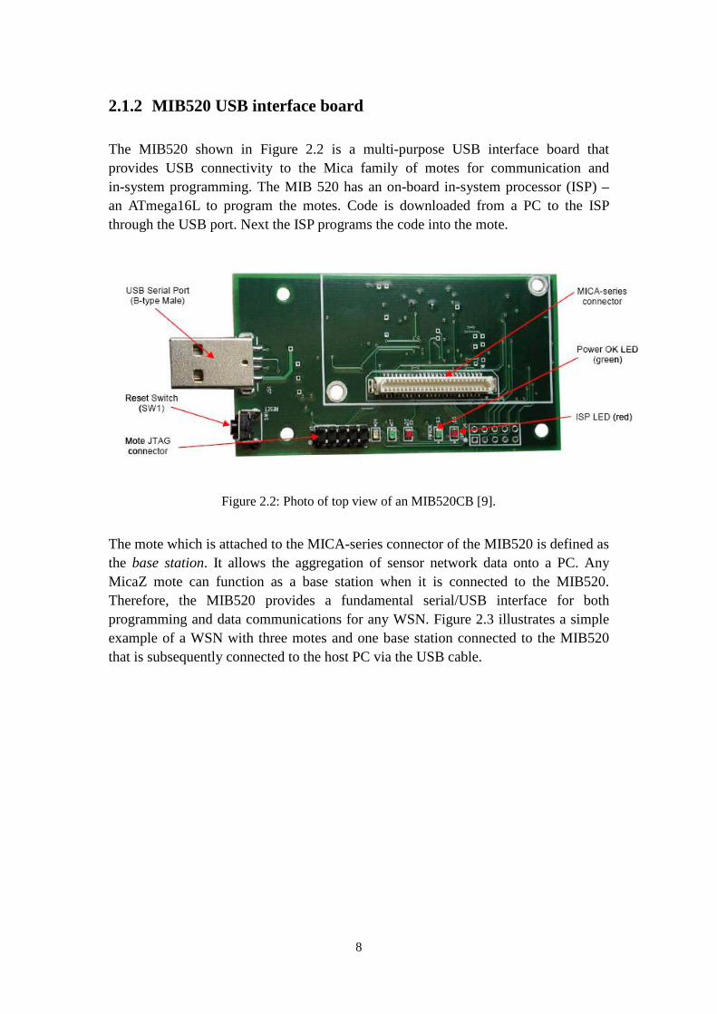
2.1.2 MIB520 USB interface board

The MIB520 shown in Figure 2.2 is a multi-purpose USB interface board that provides USB connectivity to the Mica family of motes for communication and in-system programming. The MIB 520 has an on-board in-system processor (ISP) – an ATmega16L to program the motes. Code is downloaded from a PC to the ISP through the USB port. Next the ISP programs the code into the mote.

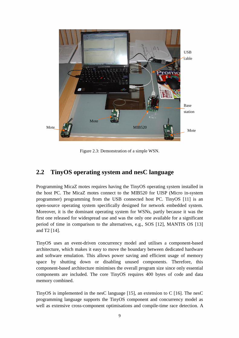
The mote which is attached to the MICA-series connector of the MIB520 is defined as the base station. It allows the aggregation of sensor network data onto a PC. Any MicaZ mote can function as a base station when it is connected to the MIB520. Therefore, the MIB520 provides a fundamental serial/USB interface for both programming and data communications for any WSN. Figure 2.3 illustrates a simple example of a WSN with three motes and one base station connected to the MIB520 that is subsequently connected to the host PC via the USB cable.

Figure 2.2: Photo of top view of an MIB520CB [9].

9

2.2 TinyOS operating system and nesC language

Programming MicaZ motes requires having the TinyOS operating system installed in the host PC. The MicaZ motes connect to the MIB520 for UISP (Micro in-system programmer) programming from the USB connected host PC. TinyOS [11] is an open-source operating system specifically designed for network embedded system. Moreover, it is the dominant operating system for WSNs, partly because it was the first one released for widespread use and was the only one available for a significant period of time in comparison to the alternatives, e.g., SOS [12], MANTIS OS [13] and T2 [14]. TinyOS uses an event-driven concurrency model and utilises a component-based architecture, which makes it easy to move the boundary between dedicated hardware and software emulation. This allows power saving and efficient usage of memory space by shutting down or disabling unused components. Therefore, this component-based architecture minimises the overall program size since only essential components are included. The core TinyOS requires 400 bytes of code and data memory combined. TinyOS is implemented in the nesC language [15], an extension to C [16]. The nesC programming language supports the TinyOS component and concurrency model as well as extensive cross-component optimisations and compile-time race detection. A

Figure 2.3: Demonstration of a simple WSN.

USB

cable

MIB520

Base

station

Mote

Mote Mote

10

complete TinyOS system consists of a tiny scheduler and a graph of components, each of which is an independent computational entity that exposes one or more interfaces. There are two types of components in nesC: modules and configurations. Any component can provide and also use interfaces. Modules provide application code, implementing one or more interfaces. Configurations are used to wire other components together, connecting interfaces used by components to interfaces provided by others. Applications written in nesC that run on wireless sensor motes are built by writing and assembling different components as required. The interfaces are the only point of access to the component, and they are also bidirectional: they contain commands and events. Commands and events are mechanisms for inter-component communication. A command is typically a request to a component to perform some service, such as initiating a sensor reading, while an event signals the completion of that service. Events may also be signaled asynchronously, for example, due to hardware interrupts or message arrival. From a traditional OS perspective, commands are analogous to downcalls and events to upcalls. Generally speaking, every nesC application is described by a top level configuration that wires together the components used. This arrangement is shown in Figure 2.4.

TinyOS as well as nesC provide a revolutionary solution for networked embedded systems such as motes by implementing an efficient framework for modularity and a resource-constrained, event-driven concurrency model. TinyOS is by no means a finished system. It continues to evolve and grow, and the latest version of TinyOS is

A generic application

Main StdControl

StdControl

StdControl

StdControl

StdControl

Component 1

Component 2

Component M

Other interfaces

Other interfaces

Other interfaces

Component

(application

code) Other interfaces

Figure 2.4: Top level configuration for a generic application, where the

interfaces in red are provided by components and the interfaces in blue

are used by components.

11

TinyOS 2.x. During the time when the proposed auto-calibration system was developed, TinyOS 1.1.15 and nesC 1.1-1w were used.

2.3 MATLAB and measurement instruments

It is very useful for us to be able to interact with a wireless mote or sensor network using MATLAB. MATLAB is a powerful matrix-based programming language with a number of libraries available for plotting and analysing data. It provides a command-like environment from which users can send or receive messages to or from their WSN and analyse data after collection. Users can also use all of TinyOS’s Java tools from within the MATALB environment for easy visualisation and manipulation of incoming and outgoing data. In addition to this, MATLAB provides a very rich library of toolboxes to users for various purposes. The version of MATLAB used here is 7.5.0.342 (R2007b). The ultimate goal of the proposed automated calibration system is to control every component using MATLAB in order to establish calibration lookup tables for both receive and transmit motes. The utilisation of the Instrument Control Toolbox built in MATLAB makes it possible to interact with the measurement instruments involved. The Instrument Control Toolbox of version 2.5 lets users communicate with instruments, such as oscilloscopes, function generators, and analytical instruments, directly from MATLAB. With the toolbox, users can generate data in MATLAB to send out to an instrument, or read data into MATLAB for analysis and visualisation. The toolbox realises the communication between MATLAB and instruments by providing a consistent interface to all devices independent of hardware manufacturer, protocol, or driver. Generally speaking, the Instrument Control Toolbox provides three ways to communicate with instruments, including: Instrument drivers : The toolbox supports VXIplug&play, IVI, and MATLAB

instrument drivers. VXIplug&play and IVI instrument drivers often ship with instruments and are also available from the instrument manufacturers’ web sites. MATLAB instrument drivers can be created by using driver development tools provided in the Instrument Control Toolbox. The biggest advantage of this approach is that learning instrument-specific commands, such as Standard Commands for Programmable Instruments (SCPI), is avoided and common MATLAB terminology is used to interact with instruments.

Communication protocols: The toolbox supports communication protocols, including GPIB, serial, TCP/IP, and UDP, for directly communicating with instruments. Alternatively, instruments can be accessed by using Virtual Instrument Software Architecture (VISA) [17] over GPIB, VXI, USB, TCP/IP, and serial buses. The SCPI is required to control programmable test and measurement devices.

Test and Measurement Tool: This is the GUI which allows users to communicate with and configure instruments without writing code. This tool can

12

also automatically generate M-code from instrument control sessions for fine-grained modification.

In our application, MATLAB needs to control two types of measurement instruments, specifically the Agilent E4432B ESG-D3000B RF signal generator and the Anritsu MS2721A spectrum analyser. The signal generator operates over a frequency range from 250 kHz to 3 GHz, and it uses a USB/GPIB interface that enables fast and direct communication between the host PC and the instrument. Therefore, MATLAB can send commands to the signal generator via the USB/GPIB bus. The spectrum analyser is small, portable and easy to use with measurement capability for applications up to 7.1 GHz. It is used as a part of the automated calibration system for Tx motes, and a direct Ethernet connection via a RJ-45 cable is required to connect the spectrum analyser to the PC for programming the instrument and capturing the measured data into MATLAB.

3 Design

The automated calibration system for wireless sensor motes proposed in this report consists of two subsystems. One is for the mote receiver and the other one is for the mote transmitter. The calibration procedure for both receiver and transmitter can be carried out in an unattended manner by running MATLAB programs to schedule the process. Although the automated calibration system was initially developed for MicaZ motes from Crossbow Technology Inc., this generic method can also be easily extended and applied to any other platforms from different vendors, provided they have a RF connector. The methodology is detailed in the subsequent sections.

3.1 Auto-calibration subsystem for the mote receiver

The analysis of the mote RF performance is based on the precise measurement of metadata RSSI values. They are generated at the hardware level of the CC2420 transceiver of an Rx mote. Subsequently, we see that this parameter is hardware dependent and varies from one mote to another. In our automated calibration subsystem for the Rx mote, we designed a system that eliminates the hardware dependency by creating an accurate relationship between the RSSI values and the actual received power at the Rx mote antenna connector. As can be seen in Figure 3.1,

13

in normal use the Rx mote at the base station receives RF signals, measures the RSSI values that are conveyed to the host PC via a USB interface. The Rx mote has an MMCX connector which is usually attached to a one-quarter wavelength monopole whip antenna. The RSSI values are computed in the mote hardware and are provided as a digital value that can be read from the 8 bit, signed 2’s complement RSSI.RSSI_VAL register. It is averaged over 8 symbol periods (128 µs), in accordance with [18]. In the MicaZ specifications, the RSSI register value RSSI.RSSI_VAL is referred to the power P at the RF connector by:

OFFSETRSSIVALRSSIP __ += [dBm] (1)

where the RSSI_OFFSET is found empirically during system development from the front end gain. From the specifications, RSSI_OFFSET is approximately -45. Subsequently, this will result in a hardware dependence of the estimated received power P due to the use of the empirical offset value and the assumed linear behaviour of the RSSI characteristic. In addition, the manufacturer’s data sheet [10] states that the RSSI accuracy is specified as 6± dB. In order to use the MicaZ as a measurement instrument we need to improve the accuracy of the RSSI values as an estimate of the received power P.

Rx mote

(BS) RSSI PC

Whip antenna

MMCX connector

Rx mote

(BS) RSSI PC

MMCX connector

USB cable

USB cable

1 2

Figure 3.1: Top: the Rx mote is usually attached to a whip antenna.

Bottom: the whip antenna is disconnected from the MMCX

connector.

14

To reduce the uncertainty in the measurement of power P, we disconnect the antenna from the mote as shown in Figure 3.1 (bottom) and connect this port to a RF signal generator that provides accurately known RF power levels at the mote input. This permits us to map the input power P to the indicated RSSI values given by the mote. This mapping is stored in the form of a look-up table that permits us to map RSSI values to accurate values of P and so mitigate the uncertainty of the input power P. The signal generator has been chosen for the following reasons:

• It provides accurately known levels of input power P at the Rx mote antenna connector.

• The signal generator can deliver a wide range of power output levels that permits calibration over a wide range of mote input power.

• We are not reliant on the calibration of the Tx mote. Figure 3.2 displays the top level configuration of the auto-calibration subsystem for the mote receiver.

For our measurement application we need to calibrate the RSSI for all the 16 available frequency channels from channel 11 (2.405 GHz) to channel 26 (2.480 GHz) in steps of 5 MHz. Therefore, this requires the calibration of the Rx mote over these channels by establishing 16 lookup tables. The automated calibration system shown in Figure 3.2 uses a PC with MATLAB installed to control a signal generator while the PC also logs the RSSI_VAL register values from the Rx mote under test. On each frequency channel, the PC sends commands to increment the output power of the

PC

MATLAB

USB

cable

Received

Packets

Rx mote

(BS)

RG316

Coaxial cable S

1

2

Power

Splitter

USB/GPIB

Commands sent from

MATLAB

Signal

Generator

Tx

mote

RG316

Coaxial cable

Figure 3.2: Top level configuration of the auto-calibration subsystem for

the mote receiver, where the solid arrows represent the direction of data

flow.

Connector

MMCX connector

15

signal generator from -100 dBm to -20 dBm in steps of 1 dBm in order to cover the expected range of input powers at the Rx mote antenna connector. The Rx mote that is acting as the base station is directly connected to the PC via a USB port. The Tx mote sends valid packets all the time via the coaxial cables to ensure that the Rx mote under test can capture the receive data and transfer it to the PC. To do this a combiner (power splitter) is used to combine the signal generator output with the Tx mote output prior to application to the Rx mote under test. All valid received packets contain the RSSI_VAL register values generated by the hardware. These values directly relate to the received “background noise” which in this case is actually the known signal power from the signal generator. The values are combined with the data corresponding with the valid received packets and then logged by the PC. The output power from the signal generator is increased in steps of 1 dBm whenever MATLAB receives 8 valid packets from the Rx mote. This ensures that each RSSI_VAL register value can always be associated with the corresponding input power P at the Rx mote antenna connector. However, the utilisation of the power splitter and one piece of coaxial cable (RG316) between the signal generator output and the Rx mote MMCX connector introduces some insertion loss which needs to be accounted for by using a correction factor. Therefore, the actual input power at the Rx mote MMCX connector is given by:

splitterpowcablegensig LLPP __ −−= [dBm] (2)

where P is the input power at the Rx mote antenna MMCX connector, Psig_gen is the output power from the signal generator, Lcable is the coaxial cable loss, and Lpow_splitter is the power splitter loss.

3.1.1 Message format

The actual format of the messages that are transmitted and received between the Tx mote and the Rx mote in our calibration process is illustrated in Figure 3.3 (a), and the actual format of the messages that are sent from the Rx mote (BS) to the host PC is illustrated in Figure 3.3 (b).

16

Bytes: 2 2 10

Number of packets Source

node 0xFF … … … 0xFF

Bytes: 2 2 1 1 8

Number of packets Source

node RSSI_VAL Status byte 0xFF … 0xFF

The messages generated and transferred from the Rx mote to the host PC contain all the necessary information for establishing the lookup tables. The total length of one packet message is 14 bytes. The first two bytes are the counter values that are incremented by one once the message is released successfully by the radio at the Tx mote. The next two bytes are the source node indicating the node number of the Tx mote. This is defined at the compile time. The RSSI_VAL register value is generated by the Rx mote hardware and uses a 1 byte signed 2’s complement format. The RSSI_VALID status bit is located at the second bit in the status byte, and it indicates when the RSSI value is valid. This information is generated every time a packet is received at the Rx mote. When it is set to ‘1’, this indicates that the receiver has been enabled for at least 8 symbol periods [10]. In TinyOS 1.x there is no supported interface for direct acquisition of RSSI_VAL register values and status byte. The only way we found to read them is to apply the following commands simultaneously:

call HPLCC2420.cmd(0) (C1) call HPLCC2420.read(0x13) (C2)

The first command reads the status byte at address 0x0 that identifies whether the RSSI_VALID bit is valid. The next command reads the ‘background noise’ power value stored in RSSI_VAL register. Note that RSSI_VAL register values are located in the lower 8 bits of address 0x13. Once the RSSI_VAL register value is computed and read out from the hardware, it is then included within the received packet to be transferred back to the host PC for construction of the lookup tables. During the post-processing required for constructing the Rx lookup tables, the packets are discarded if their corresponding RSSI_VALID status bits are set to ‘0’.

Figure 3.3: (a) Format of messages actually transmitted and

received between Tx mote and Rx mote over the radio. (b) Format

of messages actually transmitted and received between BS and host

PC.

(b)

(a)

17

3.1.2 Clear Channel Assessment threshold

The Clear Channel Assessment (CCA) signal is determined by comparing the measured RSSI value with a programmable threshold value. The CCA function is used to implement the CSMA-CA functionality specified in [18]. The CC2420 transceiver checks whether the radio channel is clear before attempting a transmission of a packet by looking to see if the interference from other transmitters is above the threshold. It does this to avoid causing interference and packet loss to other motes. The carrier sense threshold level is programmed using RSSI.CCA_THR which is located in the upper 8 bits at the register address 0x13. The CCA threshold value is represented as a signed 2’s complement number. The CCA signal goes active when the received signal is below the threshold. The default value of CCA is approximately -77 dBm. However, this value is inappropriate in our proposed auto-calibration system for the motes. The Rx mote needs to be calibrated for a wide range of received power (i.e., signal generator output power), therefore, at the Tx mote either the CCA function has to be disabled or the CCA threshold has to be increased. The most straightforward way is to increase the CCA threshold to -10 dBm. Thus the signal generator can now sweep its output power from -100 dBm to -20 dBm without preventing the Tx mote from transmitting and so disabling reception at the Rx mote. This is accomplished by modifying the following code in TinyOS 1.x module CC2420ControlM.nc:

where ‘23’ is the reset value of the CCA_THR in hexadecimal, and the ‘80’ is the reset value of the RSSI_VAL. Subsequently, the revised CCA threshold for the calibration purpose is now -10 dBm after adding the RSSI_OFFSET of -45 to 0x23.

3.1.3 Applications running on Tx and Rx motes

In the auto-calibration subsystem for the Rx mote under test the appropriate application programs must be running on both Tx and Rx motes to ensure the correct data flow. The application which runs on the Tx mote is compiled to be an executable file based on four main files, i.e., the configuration file CountDualC.nc, the module file CountDualM.nc, the header file CountMsg.h, and the make file makefile. The frequency needs to be changed in the makefile for each channel calibration. The application which runs on the Rx mote is also compiled to be an executable file based on four main files, i.e., the configuration file TOSBase.nc, the module file

gCurrentParameters[CP_RSSI] = 0x2380 (C3)

CCA_THR [7:0]

RSSI_VAL [7:0]

18

TOSBaseM.nc, the header file CountMsg.h, and the make file makefile. The frequency also needs to be synchronised with the that for the Tx mote by manually setting the parameter in the makefile.

3.1.4 Control program for the signal generator

The signal generator must be controlled from within MATLAB environment via the GPIB communication protocol, since the supported instrument driver for the Agilent E4432B ESG-D3000B series is not available at present. The signal generator transmits an unmodulated RF carrier frequency on one of 16 channels at a time. The signal generator output power lies in the range from -100 to -20 dBm. The signal generator only increments its transmit power by a 1 dB step if 8 valid packets from the Rx mote under test are received. Otherwise, the signal generator remains at its current power output. The can be viewed in the simplified flow chart of Figure 3.4.

The output power from the signal generator is recorded in a matrix along with the RSSI_VAL register values by MATLAB for the construction of the lookup tables.

3.2 Auto-calibration subsystem for the mote transmitter

The auto-calibration subsystem for the mote transmitter consists of three main components: a host PC with MATLAB installed, a spectrum analyser, and the mote

Number of packets 8≤ true

Signal generator power ++

false

Figure 3.4: Simplified flow chart of programming the signal

generator.

19

transmitter under calibration. Figure 3.5 shows the overview of the automatic calibration subsystem for the transmitting mote.

The Tx mote transmits the modulated packets by using the software defined transmit power (usually the maximum) for each of the 16 available radio channels. The frequency channel is incremented at a time interval of 5 minutes in order that the transmitted power is stable. MATLAB requests the spectrum analyser to measure the mote Tx power and then logs the returned values. Note that the max hold feature is used on the spectrum analyser since the Tx mote does not transmit continuously, i.e., there are gaps between the transmitted packets. Consequently, the lookup table of the measured transmit power from the Tx mote’s antenna connector can be established by recording the actual transmitted powers at each of the 16 radio frequency channels. The Tx mote needs to be operated in transmit mode all the time, and the message format is the same as that used for the auto-calibration subsystem of the Rx mote explained in Section 3.1.1. The RG316 coaxial cable with a length of 1 m is used to connect the Tx mote to the spectrum analyser. Therefore, the insertion loss of this cable must be taken into account when calculating the output power from the Tx mote connector. This is done by using Equation 3:

cablemeasuredTx LPP += [dBm] (3)

where PTx is the output power from the Tx mote connector, Pmeaured is the measured transmit power at the input of the spectrum analyser, and Lcable is the cable loss.

3.2.1 Calibration program running on the Tx mote

A dedicated application program runs on the Tx mote to enable the transmission of packets from the Tx mote under test. The transmission interval of packets is defined to be 0.25s, and the Tx mote changes the carrier frequency from 2.405 GHz (channel 11)

PC

MATLAB

Spectrum

Analyser Tx

RG316

Coaxial cable

Commands sent

from MATLAB

Measured Tx power

into MATLAB

Figure 3.5: Overview of the automatic calibration subsystem for the

transmitting mote, where the solid arrows represent the direction of

data flow.

Ethernet link

MMCX connector

20

to 2.480 GHz (channel 26) in steps of 5 MHz every 5 minutes. This requires the frequency change timer to be set to an interval of 5 minutes to trigger the frequency channel increment. In TinyOS 1.x, the TimerC.nc module used to create the timer for the application is claimed to have the interface Timer having a maximum interval specified by an unsigned 32 bit number, where an increment in the counter occurs once per clock tick, and 1024 ticks are equal to 1 second. However, this is not correct in practice. From investigations it appears that a more reasonable maximum time interval of the Timer interface is specified by an unsigned 16 bit number which is approximately 1 minute. This does not satisfy the requirements of our calibration program, and the Tx mote stops transmitting once the timer increases to a value beyond this limit. Therefore, nested timing loops have been implemented to overcome this problem. Specifically, two timers, namely Timer 1 and Timer 2, are used in the application program. Timer 1 expires every 30s and increments the counter by 1. When the counter reaches 8, the program will initiate Timer 2 and stop Timer 1. Timer 2 then triggers the frequency change when it expires, and the program restart Timer 1. The resultant time will be 5 minutes. The design of the application comprises four files, namely the configuration CountDualTxC.nc, the module CountDualTxM.nc, the header file CountMsg.h, and the make file Makefile.

3.2.2 Control program for the spectrum analyser

The Anritsu MS2721A spectrum analyser can be connected to the host PC shown in Figure 3.5 using a USB connection or a Direct Ethernet connection. It has been confirmed by the Anritsu manufacturing division that the MS2721A can only be controlled by the VISA I/O library (that is mentioned in Section 2.3) over the Ethernet link. Therefore, the SCPI commands [19] written in MATLAB M-file can be sent to the signal generator over the TCP/IP bus. The algorithm of this control program is explained in Figure 3.6.

21

The spectrum analyser needs to be operating at the same frequency channel on which the Tx mote is transmitting. It records the measured input power at the end of every 5 minute interval and returns it to the host PC. Therefore, the timing issue must be taken into account when the spectrum analyser and the Tx mote under test are working together, since they function individually without communicating with each other. MATLAB should start sending the control program to the spectrum analyser immediately after the Tx mote is switched on for transmission. The control program is named as calibrate_Tx_final.m. It is written in MATLAB M-file using SCPI commands.

Initialise the

spectrum analyser

Timer 5≤ minutes

Acquire the measured transmit

power, and increment the frequency

false

true

Figure 3.6: Flow chart of control program which MATLAB uses to

send commands and acquire data to and from the spectrum analyser.

22

4 Implementation of auto-calibration subsystem for

the mote receiver

4.1 Output power characteristics of the signal generator

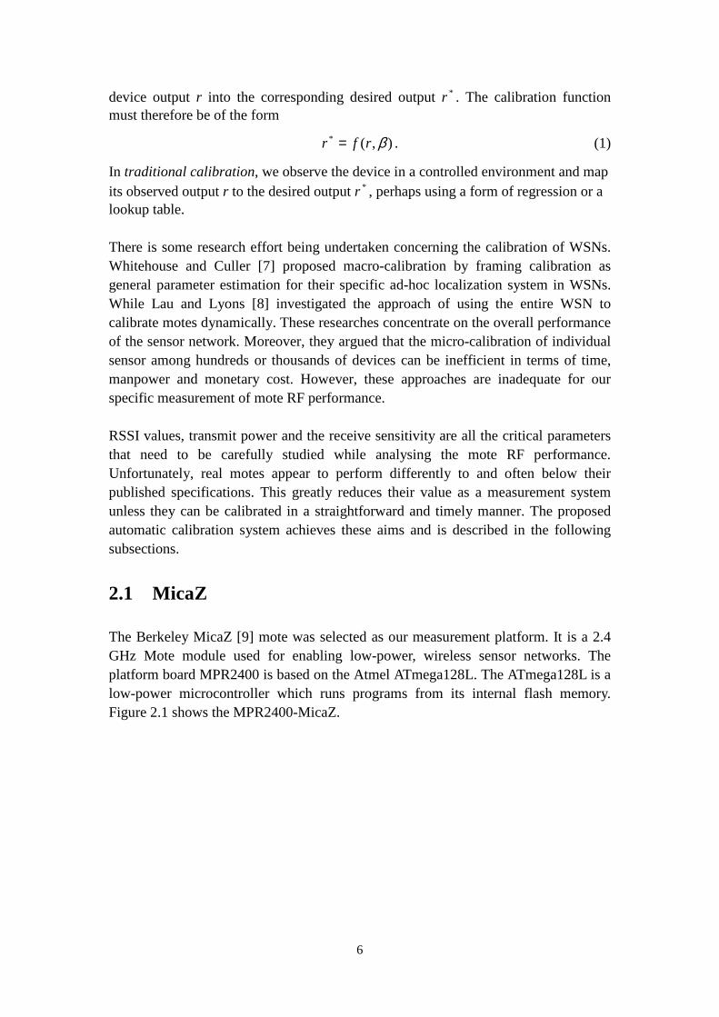
It is important to measure the output power characteristics of the signal generator across the frequency channels of interest in order to ensure that it does not have any effect on the automated calibration subsystem shown in Figure 3.2. To achieve this, the signal generator is connected to the spectrum analyser directly using only two low loss adaptors. The signal generator transmits an unmodulated carrier with the output power set to 0 dBm. The output power characteristic of the signal generator is displayed in Figure 4.1.

It can be seen that the measured output power of the signal generator has a maximum value of -0.36 dBm and a minimum value of -0.50 dBm over the frequency band of interest. The insertion loss of the adaptors is negligible. Generally speaking, the signal generator has a flat response in frequency, i.e., it does not vary significantly as the frequency changes from channel 11 (2.405 GHz) to channel 26 (2.480 GHz).

Figure 4.1: Output power characteristics of the signal generator

across 16 frequency channels, where the nominal output power is

set to 0 dBm. The unit along y-axis is in dBm.

23

4.2 Frequency response and insertion loss of the power

splitter

The power splitter used in the system is the Mini-Circuits ZN2PD2-50+ [20]. It is specified for operation over a frequency range from 500 to 5000 MHz. It has three ports, namely SUMPORT (marked as S), PORT 1 (marked as 1), and PORT 2 (marked as 2), as shown in Figure 3.2. The signal from the Tx mote into port 1 and the signal from the signal generator into port 2 is combined and output from port S is connected to the base station. In order to obtain the power P at the Rx mote antenna connector, the attenuation loss due to the insertion of the splitter in Equation 2 has to be accounted for. Indeed, any non-flatness in the frequency response could eventually be compensated for if required.

The loss of the power splitter between port 2 and port S as a function of frequency is measured by inserting the power splitter between the spectrum analyser and the signal generator, while Port 1 is connected to a 50Ω termination. The transmit power of the signal generator is set to -10 dBm.

Figure 4.2 shows a very clear drop in the measured power at port S compared to the

Figure 4.2: Frequency response of the power splitter

ZN2PD2-50+ across 16 frequency channels, where the default

output power of the signal generator is -10 dBm. The y-axis is in

dBm.

24

-10 dBm level applied at port 2. It also shows a flat response across all 16 frequency channels. The average insertion loss that the power splitter contributes to the automated calibration subsystem for the Rx mote under test is approximately 4.0 dB.

4.3 Frequency response and insertion loss of the RG316

coaxial cable

The RG316 coaxial cable is one metre long, and it is used to connect power splitter port S to the Rx mote connector. The term Lcable in Equation 2 describes the attenuation loss which the coaxial cable contributes to the whole system. However, it is very difficult to measure the practical frequency response and insertion loss of the coaxial cable separately due to its incompatible connectors with those on the spectrum analyser and the signal generator. Consequently, the frequency response of the one metre coaxial cable is assumed to be flat and according to the manufacturers’ data sheet has an attenuation of 1.54 dB/m [21]. Table 4.1 summarises all the components which contribute insertion loss to the system shown in Figure 3.2.

The components Terms in Equation 2 Attenuation

loss (dB)

Power splitter (between Port 2 and Port S) Lpow_splitter 4.00

RG316 coaxial cable (One metre) Lcable 1.54

Total loss Ltotal 5.54

Ltotal is the correction factor which must be subtracted from the transmit power defined by the signal generator in order to calculate the input power P at the Rx mote connector according to Equation 2.

4.4 Lookup tables for the mote receiver under test

The Tx mote transmits packets at time intervals of 0.25s. The signal generator will not increment its transmit power until the MATLAB code at the PC successfully receives and logs 8 packets from the Rx mote under test. The actual input power P can be computed by subtracting the total loss Ltotal from the Psig_gen within MATLAB for every packet received. RSSI_VAL can be read directly from the fifth byte of the message defined in Section 3.3. This process must be repeated 16 times, once for each of 16 frequency channels. Therefore, the lookup tables can be established by plotting

Table 4.1: Summary of components which make the contribution of the

attenuation loss to the auto-calibration subsystem for the Rx mote under

test, where the middle column lists their corresponding terms described in

Equation 2.

25

the Pinput values against the RSSI_VAL values. In our experiment the MicaZ mote labeled as Surge 6 is used for the Rx mote under test, and the MicaZ mote labeled as Surge 7 is used for the Tx mote.

4.4.1 Raw lookup tables for the mote receiver under test

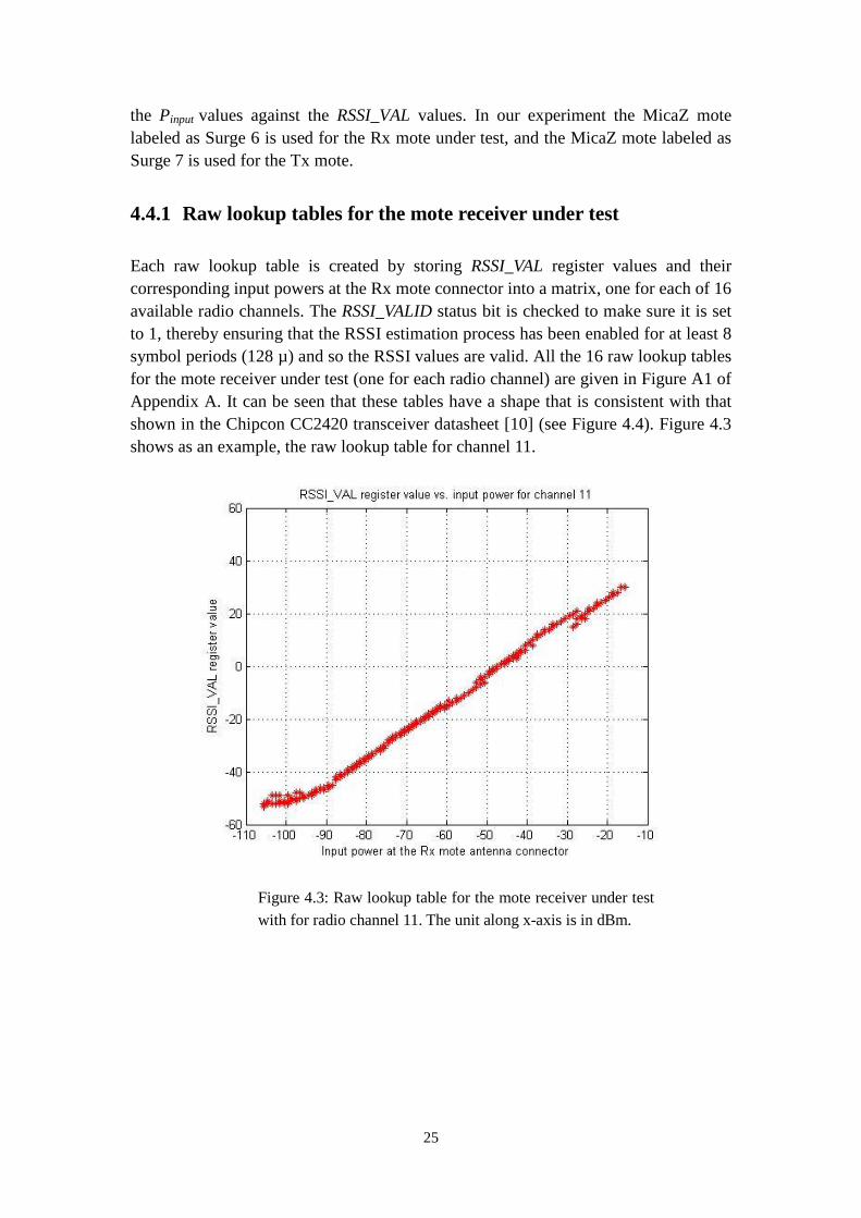
Each raw lookup table is created by storing RSSI_VAL register values and their corresponding input powers at the Rx mote connector into a matrix, one for each of 16 available radio channels. The RSSI_VALID status bit is checked to make sure it is set to 1, thereby ensuring that the RSSI estimation process has been enabled for at least 8 symbol periods (128 µ) and so the RSSI values are valid. All the 16 raw lookup tables for the mote receiver under test (one for each radio channel) are given in Figure A1 of Appendix A. It can be seen that these tables have a shape that is consistent with that shown in the Chipcon CC2420 transceiver datasheet [10] (see Figure 4.4). Figure 4.3 shows as an example, the raw lookup table for channel 11.

Figure 4.3: Raw lookup table for the mote receiver under test

with for radio channel 11. The unit along x-axis is in dBm.

26

4.4.2 Lookup tables after averaging and rounding

Because the input power P impinging at the Rx mote connector does not increment until eight packets have been successfully received by the base station, these eight packets all have the same input power. Therefore, to reduce the effect of measurement noise at the receiver we choose to calculate the average of the eight RSSI_VAL register values logged at the PC that correspond to the same input power. By default MALTAB would return the mean value of these to four decimal places. However, this is rounded to the nearest integer value so that it has the same format as that originally read from the mote register. The processing of the 16 raw lookup tables is illustrated in Figure 4.5. Every raw table must go through two processing blocks, i.e., averaging and rounding. Figure 4.6 shows one of the 16 (actually for channel 11) lookup tables after the process of averaging and rounding respectively. All 16 sets are given in Figure A2 of Appendix A. Figure 4.6 (a) corresponds to the processed table after averaging, and Figure 4.6 (b) corresponds to the processed table after the rounding process.

Figure 4.4: Typical RSSI value vs. input

power from [10].

27

…

…

Raw table 1

Raw table 16

Averaging process block

Rounding process block

…

Figure 4.5: Processing blocks of averaging and rounding applied to the 16 raw lookup tables for the mote receiver under test.

…

…

(a)

Processed table 16

Processed table 1

28

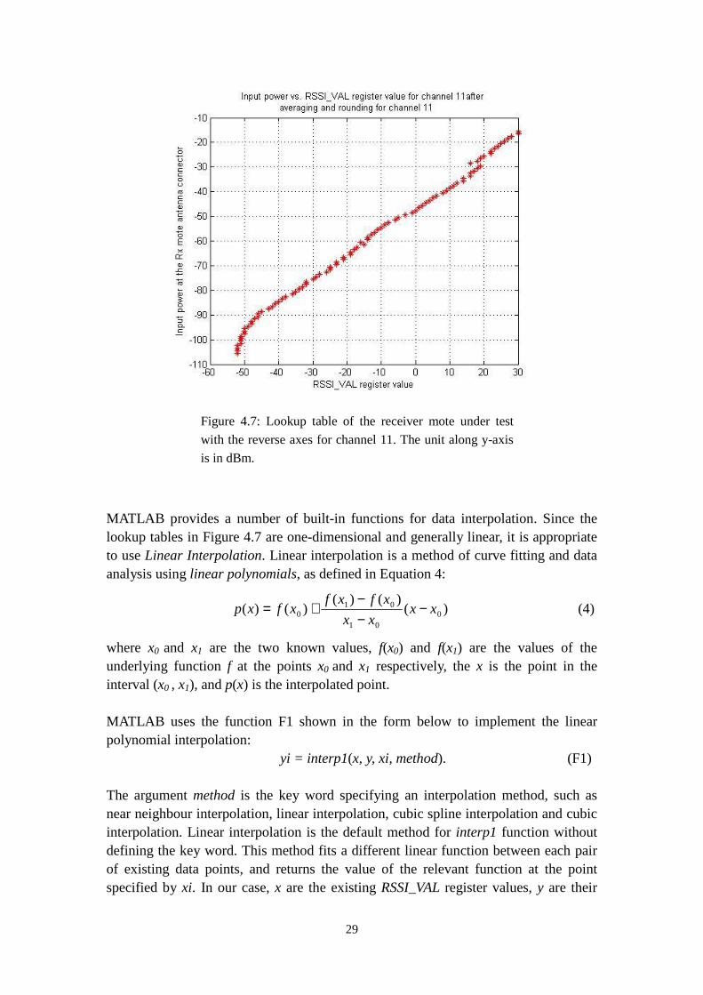
4.4.3 Lookup tables after the interpolation

It has been found that after going through the averaging and rounding process some RSSI_VAL register values are missing. This becomes more obvious in Figure 4.7 (for channel 11) when the lookup tables are plotted with the X and Y axes swapped compared with that shown in Figure 4.6. Clearly, the missing RSSI_VAL values do not have a corresponding input power P in the table. To address this problem interpolation techniques are applied to insert the missing RSSI_VAL values in order to complete the lookup tables. Consequently, we can now associate all the possible RSSI_VAL values to an input power P within the range of interest.

(b)

Figure 4.6: One of 16 sets of lookup tables after the processes

of averaging and rounding for channel 11. (a) corresponds to

the processed lookup table after averaging, and (b) corresponds

to the processed lookup table after rounding. The unit along

x-axis in both plots is in dBm.

29

MATLAB provides a number of built-in functions for data interpolation. Since the lookup tables in Figure 4.7 are one-dimensional and generally linear, it is appropriate to use Linear Interpolation. Linear interpolation is a method of curve fitting and data analysis using linear polynomials, as defined in Equation 4:

)()()(

)()( 001

010 xx

xx

xfxfxfxp −

−−

+= (4)

where x0 and x1 are the two known values, f(x0) and f(x1) are the values of the underlying function f at the points x0 and x1 respectively, the x is the point in the interval (x0 , x1), and p(x) is the interpolated point. MATLAB uses the function F1 shown in the form below to implement the linear polynomial interpolation:

yi = interp1(x, y, xi, method). (F1) The argument method is the key word specifying an interpolation method, such as near neighbour interpolation, linear interpolation, cubic spline interpolation and cubic interpolation. Linear interpolation is the default method for interp1 function without defining the key word. This method fits a different linear function between each pair of existing data points, and returns the value of the relevant function at the point specified by xi. In our case, x are the existing RSSI_VAL register values, y are their

Figure 4.7: Lookup table of the receiver mote under test

with the reverse axes for channel 11. The unit along y-axis

is in dBm.

30

corresponding input powers P, xi are the missing RSSI_VAL register values, and yi are the missing input powers P. The algorithm for finding the missing RSSI_VAL register values is explained below: Sort the existing RSSI_VAL register values into ascending order. Find the difference between adjacent elements. Search and find the position where the difference is not zero indicating missing

values. Go through a loop to compute and insert every missing RSSI_VAL register value

based on the value of difference between adjacent elements. The implementation of this algorithm in MATLAB M-file is illustrated in Figure 4.8.

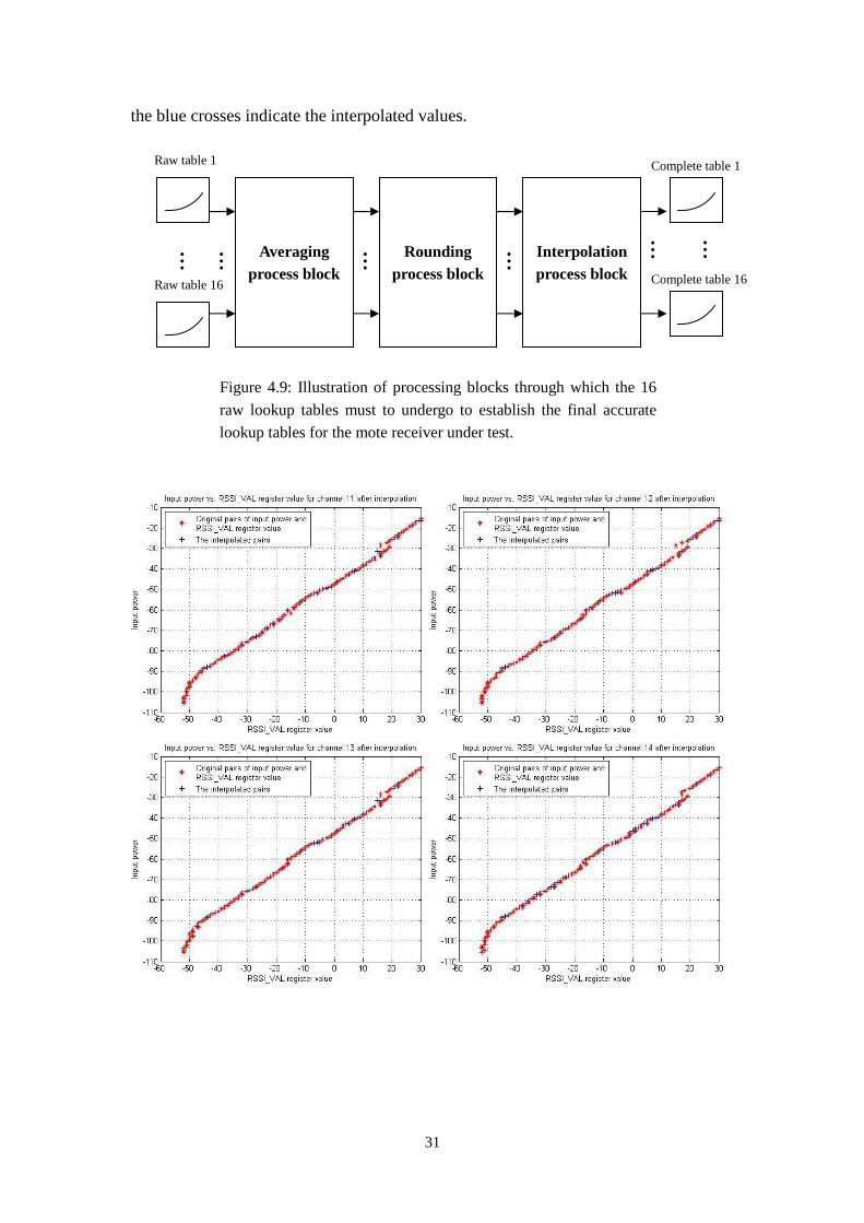
Once the missing RSSI_VAL register values are found, the function F1 must be used to interpolate the missing input powers P corresponding to the inserted RSSI_VAL values. Finally, the 16 complete lookup tables can be established after going through the processing blocks shown in Figure 4.9, and they are illustrated in Figure 4.10 where

rssi_val = sortrows(rssi_val); % Sort RSSI_VAL register value in acceding order.

function [ missing_RSSI ] = locate_missing_RSSI_reg_val (rssi_val)

% Initialise the parameters.

missing_RSSI = [];

% Find the difference between adjacent elements.

a = [1 diff(rssi_val)];

a(a = 1) = 0;

a(a>0) = a(a>0) - 1;

% Search and find the position where the missing values are.

[row col val] = find(a);

% Compute and insert every missing RSSI_VAL values based on the difference.

for m = 1:length(val)

rssi_val_col = col(1,m);

for n = 1:val(1,m)

RSSI = rssi_val(1,rssi_val_col) - n;

missing_RSSI = [missing_RSSI RSSI];

end

end

end

Figure 4.8: Illustration of the algorithm of finding the missing RSSI_VAL register values in MATLAB M-file.

31

the blue crosses indicate the interpolated values.

…

…

Raw table 1

Raw table 16

Averaging process block

Rounding process block

…

Figure 4.9: Illustration of processing blocks through which the 16

raw lookup tables must to undergo to establish the final accurate

lookup tables for the mote receiver under test.

Interpolation process block

… …

Complete table 1

Complete table 16

…

32

33

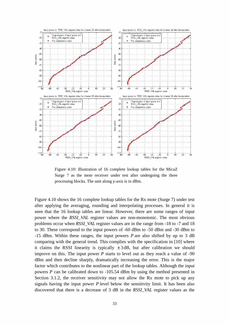
Figure 4.10 shows the 16 complete lookup tables for the Rx mote (Surge 7) under test after applying the averaging, rounding and interpolating processes. In general it is seen that the 16 lookup tables are linear. However, there are some ranges of input power where the RSSI_VAL register values are non-monotonic. The most obvious problems occur when RSSI_VAL register values are in the range from -18 to -7 and 18 to 30. These correspond to the input powers of -60 dBm to -50 dBm and -30 dBm to -15 dBm. Within these ranges, the input powers P are also shifted by up to 3 dB comparing with the general trend. This complies with the specification in [10] where it claims the RSSI linearity is typically 3± dB, but after calibration we should improve on this. The input power P starts to level out as they reach a value of -90 dBm and then decline sharply, dramatically increasing the error. This is the major factor which contributes to the nonlinear part of the lookup tables. Although the input powers P can be calibrated down to -105.54 dBm by using the method presented in Section 3.1.2, the receiver sensitivity may not allow the Rx mote to pick up any signals having the input power P level below the sensitivity limit. It has been also discovered that there is a decrease of 3 dB in the RSSI_VAL register values as the

Figure 4.10: Illustration of 16 complete lookup tables for the MicaZ

Surge 7 as the mote receiver under test after undergoing the three

processing blocks. The unit along y-axis is in dBm.

34

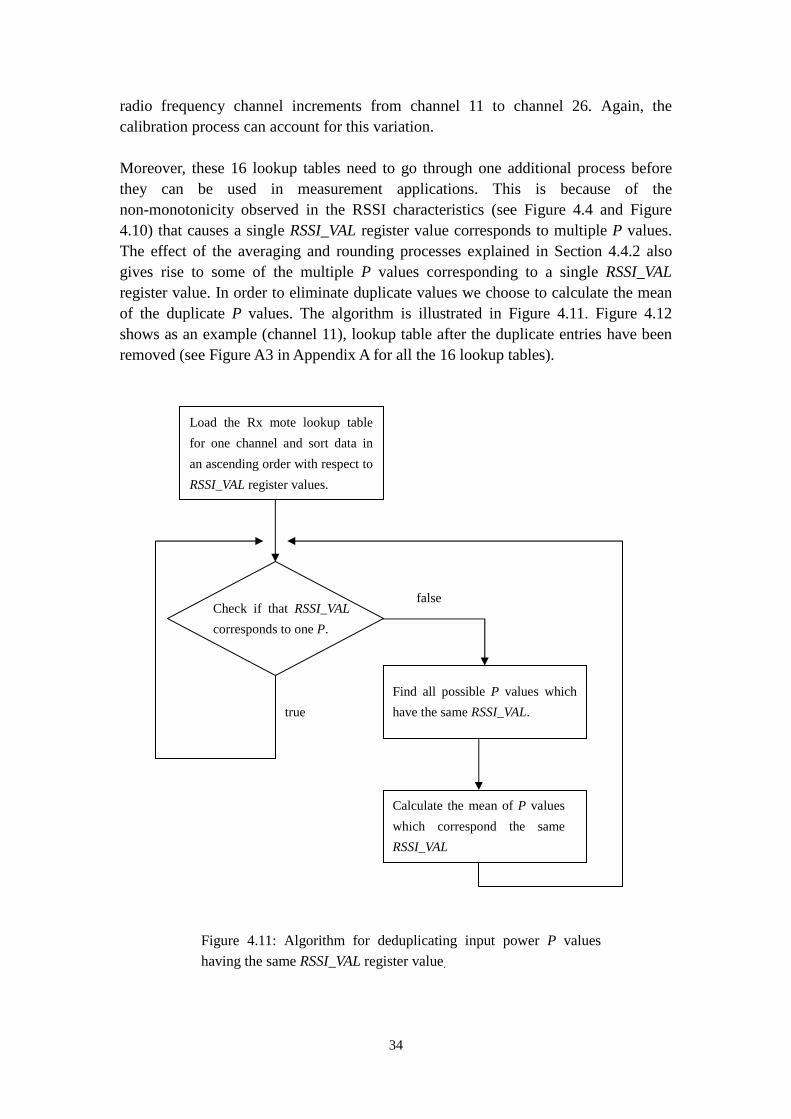
radio frequency channel increments from channel 11 to channel 26. Again, the calibration process can account for this variation. Moreover, these 16 lookup tables need to go through one additional process before they can be used in measurement applications. This is because of the non-monotonicity observed in the RSSI characteristics (see Figure 4.4 and Figure 4.10) that causes a single RSSI_VAL register value corresponds to multiple P values. The effect of the averaging and rounding processes explained in Section 4.4.2 also gives rise to some of the multiple P values corresponding to a single RSSI_VAL register value. In order to eliminate duplicate values we choose to calculate the mean of the duplicate P values. The algorithm is illustrated in Figure 4.11. Figure 4.12 shows as an example (channel 11), lookup table after the duplicate entries have been removed (see Figure A3 in Appendix A for all the 16 lookup tables).

Load the Rx mote lookup table

for one channel and sort data in

an ascending order with respect to

RSSI_VAL register values.

Check if that RSSI_VAL

corresponds to one P.

Find all possible P values which

have the same RSSI_VAL.

Calculate the mean of P values

which correspond the same

RSSI_VAL

false

true

Figure 4.11: Algorithm for deduplicating input power P values

having the same RSSI_VAL register value.

35

4.5 Lookup table for the mote transmitter under test

Figure 3.5 shows the overview of the auto-calibration subsystem for the mote transmitter under test. The transmit power was set to 0 dBm in the Tx mote. Since the Tx mote transmits modulated packets of the format defined in Figure 3.3 (a), the spectrum analyser must be set properly to measure the modulated spectrum of incoming messages. Its parameters can be set within the initialisation phase using the control program sent to the spectrum analyser from MATLAB. Table 4.2 shows the measurement parameter settings for the spectrum analyser.

Parameters Setting Parameters Setting Span 10 MHz RBW 3 MHz Auto Atten OFF VBW 3 MHz Atten Lvl 0 dB RBW/VBW 1 Reference Lvl 0 dB Preamp OFF

Table 4.2: Summary of parameter settings on the spectrum analyser for

measuring the modulated spectrum of incoming messages.

Figure 4.12: Lookup table for the Rx mote under

test after the process of deduplicating for channel

11. The unit along y-axis is in dBm.

36

Figure 4.12 shows the measured transmit power Pmeasured (see Equation 3) from the Tx mote (Surge 6) at the input of the spectrum analyser for all 16 frequency channels. However, these are the powers after the attenuation loss due to 1 m of RG316 coaxial cable as shown in Figure 3.5. The actual transmit power PTx of the Tx mote (Surge 6) under calibration is the output power at its connector, so we need to calculate it by using Equation 3. Figure 4.13 shows the final lookup table of the actual transmit power PTx for the Tx mote (Surge 6).

Figure 4.12: Measured transmitted powers from the Tx mote

(Surge 6) under test at the input of spectrum analyser across

the 16 frequency channels.

37

It can be seen from Figure 4.13 that actual transmit power at the Tx mote antenna connector varies as a function of channel number and deviates from the manufacturer’s specification. Here, the default transmit power is set at 0 dBm. In addition to the large deviation between the actual measured value and the defined value for each radio frequency channel, the actual transmit power also decreases as the radio channel number increases with a maximum variation of about 2 dB. The calibration process will considerably reduce errors owing to these issues.

5 Evaluation of the auto-calibration system

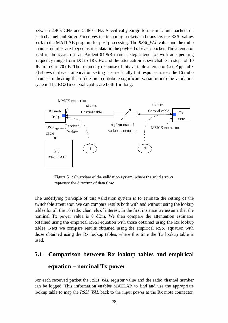
The 16 lookup tables for the mote receiver and that for the mote transmitter have been established by implementing two separate auto-calibration subsystems as explained in Section 3 and Section 4. These two subsystems form one complete auto-calibration system for the wireless sensor motes. Finally, a validation process has been developed to evaluate the overall performance of this auto-calibration system. The overview of this system is shown Figure 5.1. The validation system consists of a Tx mote, a Rx mote acting as the base station, a variable attenuator and a host PC with MATLAB installed. The Tx mote is the one labelled as Surge 6, and the Rx mote is the one labelled as Surge 7. Note that the 16 Rx lookup tables for Surge 7 and the Tx lookup table for Surge 6 have been created as described previously. Surge 6 transmits a packet every 0.25s. It also transmits for 1s on each of the 16 radio channels that lie

Figure 4.13: Final lookup table of the Tx mote (Surge 6) under

test across the 16 frequency channels.

38

between 2.405 GHz and 2.480 GHz. Specifically Surge 6 transmits four packets on each channel and Surge 7 receives the incoming packets and transfers the RSSI values back to the MATLAB program for post processing. The RSSI_VAL value and the radio channel number are logged as metadata in the payload of every packet. The attenuator used in the system is an Agilent-8495B manual step attenuator with an operating frequency range from DC to 18 GHz and the attenuation is switchable in steps of 10 dB from 0 to 70 dB. The frequency response of this variable attenuator (see Appendix B) shows that each attenuation setting has a virtually flat response across the 16 radio channels indicating that it does not contribute significant variation into the validation system. The RG316 coaxial cables are both 1 m long.

The underlying principle of this validation system is to estimate the setting of the switchable attenuator. We can compare results both with and without using the lookup tables for all the 16 radio channels of interest. In the first instance we assume that the nominal Tx power value is 0 dBm. We then compare the attenuation estimates obtained using the empirical RSSI equation with those obtained using the Rx lookup tables. Next we compare results obtained using the empirical RSSI equation with those obtained using the Rx lookup tables, where this time the Tx lookup table is used.

5.1 Comparison between Rx lookup tables and empirical

equation – nominal Tx power

For each received packet the RSSI_VAL register value and the radio channel number can be logged. This information enables MATLAB to find and use the appropriate lookup table to map the RSSI_VAL back to the input power at the Rx mote connector.

PC

MATLAB

USB

cable

Received

Packets

Rx mote

(BS)

RG316

Coaxial cable Tx

mote

RG316

Coaxial cable

Figure 5.1: Overview of the validation system, where the solid arrows

represent the direction of data flow.

MMCX connector

MMCX connector Agilent manual

variable attenuator

1 2

39

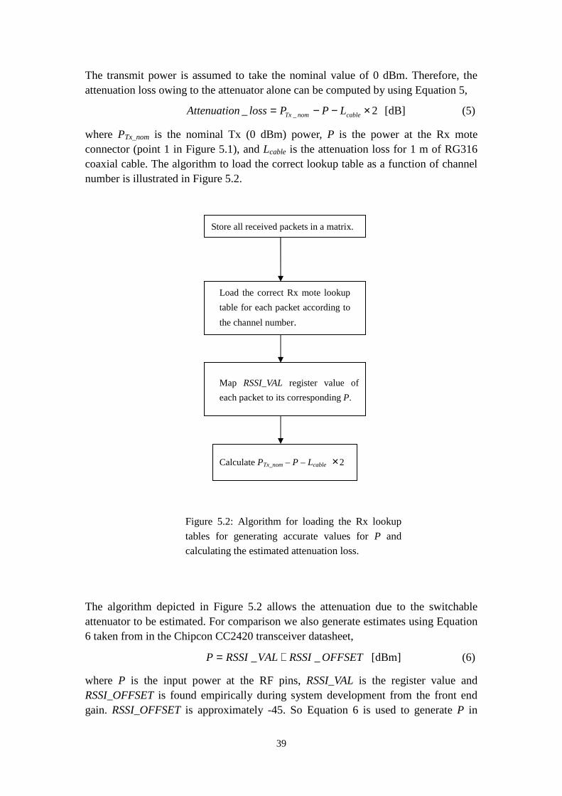
The transmit power is assumed to take the nominal value of 0 dBm. Therefore, the attenuation loss owing to the attenuator alone can be computed by using Equation 5,

2_ _ ×−−= cablenomTx LPPlossnAttenuatio [dB] (5)

where PTx_nom is the nominal Tx (0 dBm) power, P is the power at the Rx mote connector (point 1 in Figure 5.1), and Lcable is the attenuation loss for 1 m of RG316 coaxial cable. The algorithm to load the correct lookup table as a function of channel number is illustrated in Figure 5.2.

The algorithm depicted in Figure 5.2 allows the attenuation due to the switchable attenuator to be estimated. For comparison we also generate estimates using Equation 6 taken from in the Chipcon CC2420 transceiver datasheet,

OFFSETRSSIVALRSSIP __ += [dBm] (6)

where P is the input power at the RF pins, RSSI_VAL is the register value and RSSI_OFFSET is found empirically during system development from the front end gain. RSSI_OFFSET is approximately -45. So Equation 6 is used to generate P in

Store all received packets in a matrix.

Calculate PTx_nom – P – Lcable ×2

Figure 5.2: Algorithm for loading the Rx lookup

tables for generating accurate values for P and

calculating the estimated attenuation loss.

Map RSSI_VAL register value of

each packet to its corresponding P.

Load the correct Rx mote lookup

table for each packet according to

the channel number.

40

Equation 5 instead of the Rx lookup tables.

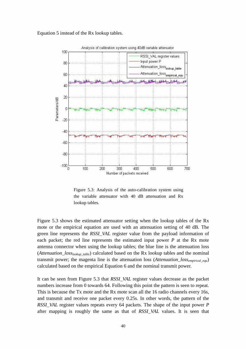
Figure 5.3 shows the estimated attenuator setting when the lookup tables of the Rx mote or the empirical equation are used with an attenuation setting of 40 dB. The green line represents the RSSI_VAL register value from the payload information of each packet; the red line represents the estimated input power P at the Rx mote antenna connector when using the lookup tables; the blue line is the attenuation loss (Attenuation_losslookup_table) calculated based on the Rx lookup tables and the nominal transmit power; the magenta line is the attenuation loss (Attenuation_lossempirical_equ) calculated based on the empirical Equation 6 and the nominal transmit power. It can be seen from Figure 5.3 that RSSI_VAL register values decrease as the packet numbers increase from 0 towards 64. Following this point the pattern is seen to repeat. This is because the Tx mote and the Rx mote scan all the 16 radio channels every 16s, and transmit and receive one packet every 0.25s. In other words, the pattern of the RSSI_VAL register values repeats every 64 packets. The shape of the input power P after mapping is roughly the same as that of RSSI_VAL values. It is seen that

Figure 5.3: Analysis of the auto-calibration system using

the variable attenuator with 40 dB attenuation and Rx

lookup tables.

41

Attenuation_losslookup_table and Attenuation_lossempirical_equ have similar responses with an approximate difference of 1.5 dB between them. However, both of them show a rise in the estimated attenuator setting at places where there is a decrease in RSSI_VAL values. Neither Attenuation_losslookup_table nor Attenuation_lossempirical_equ yield a good estimate of the actual attenuator setting of 40 dB. This is caused by not using the Tx lookup table that compensates for the variation in actual transmit power from the Tx mote as a function of the Tx channel.

5.2 Comparison between Rx lookup tables and empirical

equation – Tx lookup table

The actual transmit power on each radio channel can also be read out from the lookup table for the Tx mote based on the metadata of the radio channel number in the packet. Therefore, the attenuation loss owing to the attenuator alone can be computed by using Equation 7,

2_ __ ×−−= cabletablelookupTx LPPlossnAttenuatio [dB] (7)

where PTx_lookup_table is the transmit power at the Tx mote connector (point 2 in Figure 5.1), P is the power at the Rx mote connector (point 1), and Lcable is the attenuation loss for 1 m of RG316 coaxial cable. The algorithm to load the correct Tx and the Rx lookup tables is illustrated in Figure 5.4. The algorithm depicted in the figure allows the attenuation due to the switchable attenuator to be estimated. For comparison we also generate estimates using Equation 6 to estimate the input power P.

42

For a complete evaluation, attenuator setting estimates have been performed using the Rx lookup tables or the empirical equation at various attenuation settings from 10 dB to 70 dB. Figure 5.5 to Figure 5.11 show the performances of both schemes where the green line represents the RSSI_VAL register value from the payload information of each packet; the red line represents the estimated input power P at the Rx mote antenna connector when using the lookup tables; the blue line is the attenuation loss (Attenuation_losslookup_table) calculated based on the Tx and the Rx lookup tables; and the magenta line is the attenuation loss (Attenuation_lossempirical_equ) calculated based on the Tx lookup table and the empirical Equation 6.

Store all received packets in a matrix.

Calculate PTx_lookup_table – P – Lcable ×2

Figure 5.4: Algorithm for loading the Tx and the

Rx lookup tables for generating accurate values for

P and PTx_lookup_table and calculating the estimated

attenuation loss.

Map RSSI_VAL register value of

each packet to its corresponding

P.

Load the correct Rx mote lookup

table for each packet according to

the channel number.

Load the Tx mote lookup

table.

Search for the correct transmit

power for each packet according

to the channel number on which

the packet is transmitted.

43

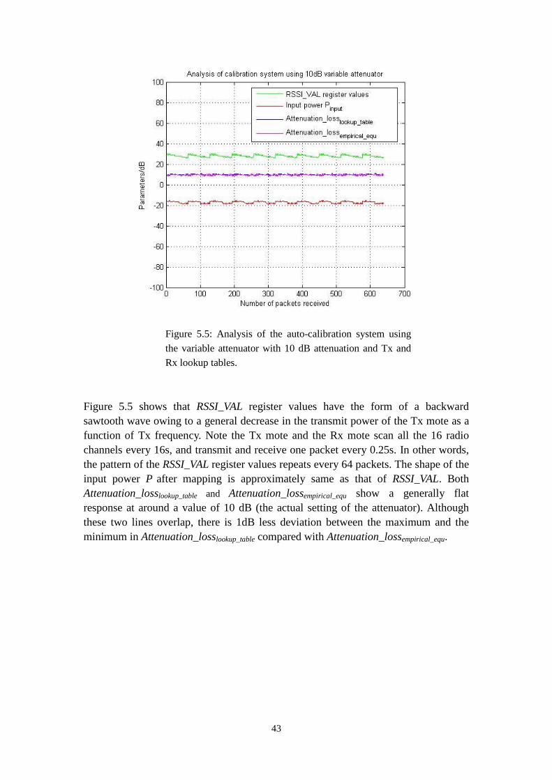
Figure 5.5 shows that RSSI_VAL register values have the form of a backward sawtooth wave owing to a general decrease in the transmit power of the Tx mote as a function of Tx frequency. Note the Tx mote and the Rx mote scan all the 16 radio channels every 16s, and transmit and receive one packet every 0.25s. In other words, the pattern of the RSSI_VAL register values repeats every 64 packets. The shape of the input power P after mapping is approximately same as that of RSSI_VAL. Both Attenuation_losslookup_table and Attenuation_lossempirical_equ show a generally flat response at around a value of 10 dB (the actual setting of the attenuator). Although these two lines overlap, there is 1dB less deviation between the maximum and the minimum in Attenuation_losslookup_table compared with Attenuation_lossempirical_equ.

Figure 5.5: Analysis of the auto-calibration system using

the variable attenuator with 10 dB attenuation and Tx and

Rx lookup tables.

44

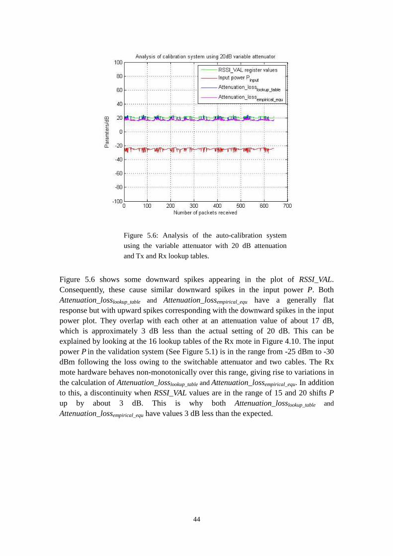
Figure 5.6 shows some downward spikes appearing in the plot of RSSI_VAL. Consequently, these cause similar downward spikes in the input power P. Both Attenuation_losslookup_table and Attenuation_lossempirical_equ have a generally flat response but with upward spikes corresponding with the downward spikes in the input power plot. They overlap with each other at an attenuation value of about 17 dB, which is approximately 3 dB less than the actual setting of 20 dB. This can be explained by looking at the 16 lookup tables of the Rx mote in Figure 4.10. The input power P in the validation system (See Figure 5.1) is in the range from -25 dBm to -30 dBm following the loss owing to the switchable attenuator and two cables. The Rx mote hardware behaves non-monotonically over this range, giving rise to variations in the calculation of Attenuation_losslookup_table and Attenuation_lossempirical_equ. In addition to this, a discontinuity when RSSI_VAL values are in the range of 15 and 20 shifts P

up by about 3 dB. This is why both Attenuation_losslookup_table and

Attenuation_lossempirical_equ have values 3 dB less than the expected.

Figure 5.6: Analysis of the auto-calibration system

using the variable attenuator with 20 dB attenuation

and Tx and Rx lookup tables.

45

Figure 5.7 shows an evident difference between Attenuation_losslookup_table and

Attenuation_lossempirical_equ despite their similar shape. The Attenuation_losslookup_table plot lies in the range from 30 dB to 32 dB with a mean value of 31.32 dB, whereas the Attenuation_lossempirical_equ plot lies in the range from 26 dB to 29 dB with a mean value of 28.16 dB. So Attenuation_losslookup_table is about 1 dB closer to the actual attenuator setting (see Appendix B) than is Attenuation_lossempirical_equ. Generally, the calculation based on the implementation of the lookup tables provides us with a more accurate result than using the empirical equation.

Figure 5.7: Analysis of the auto-calibration system

using the variable attenuator with 30 dB attenuation

and Tx and Rx lookup tables.

46

From Figure 5.8 it can be seen that Attenuation_losslookup_table achieves a better performance than Attenuation_lossempirical_equ when the switchable attenuator is set at 40 dB. The mean value of Attenuation_losslookup_table in the figure is 40.25 dB which is approximately the same as the attenuator setting of 40 dB. On the other hand, Attenuation_lossempirical_equ performs worse having a mean value of 38.53 dB, about 1.5 dB less than the actual attenuator setting. For a nominal attenuator setting of 50 dB it can be seen from Figure 5.9 that Attenuation_losslookup_table and Attenuation_lossempirical_equ give similar performances with both exhibiting repetitive fluctuations. The mean values of Attenuation_losslookup_table and Attenuation_lossempirical_equ are 47.58 dB and 48.44 dB respectively. This can be explained by looking at the lookup tables of the Rx mote in Figure 4.10, where the RSSI_VAL register values lie in the range from -13 to -8 when the attenuator is set to 50 dB. When they are mapped back to the input power P at point 1 of the validation system in Figure 5.1, the values of P lie in the range from -56 dBm to -58 dBm. This happens to be in a ‘lumpy’ range of the lookup tables. This range not only changes the linear property of the lookup tables by increasing the slope, but also contributes to the fluctuations that occur in both Attenuation_losslookup_table and Attenuation_lossempirical_equ in Figure 5.9.

Figure 5.8: Analysis of the auto-calibration system using

the variable attenuator with 40 dB attenuation and Tx and

Rx lookup tables.

47

Figure 5.10: Analysis of the auto-calibration system

using the variable attenuator with 60 dB attenuation Tx

and Rx lookup tables.

Figure 5.9: Analysis of the auto-calibration system using

the variable attenuator with 50 dB attenuation and Tx and

Rx lookup tables.

48

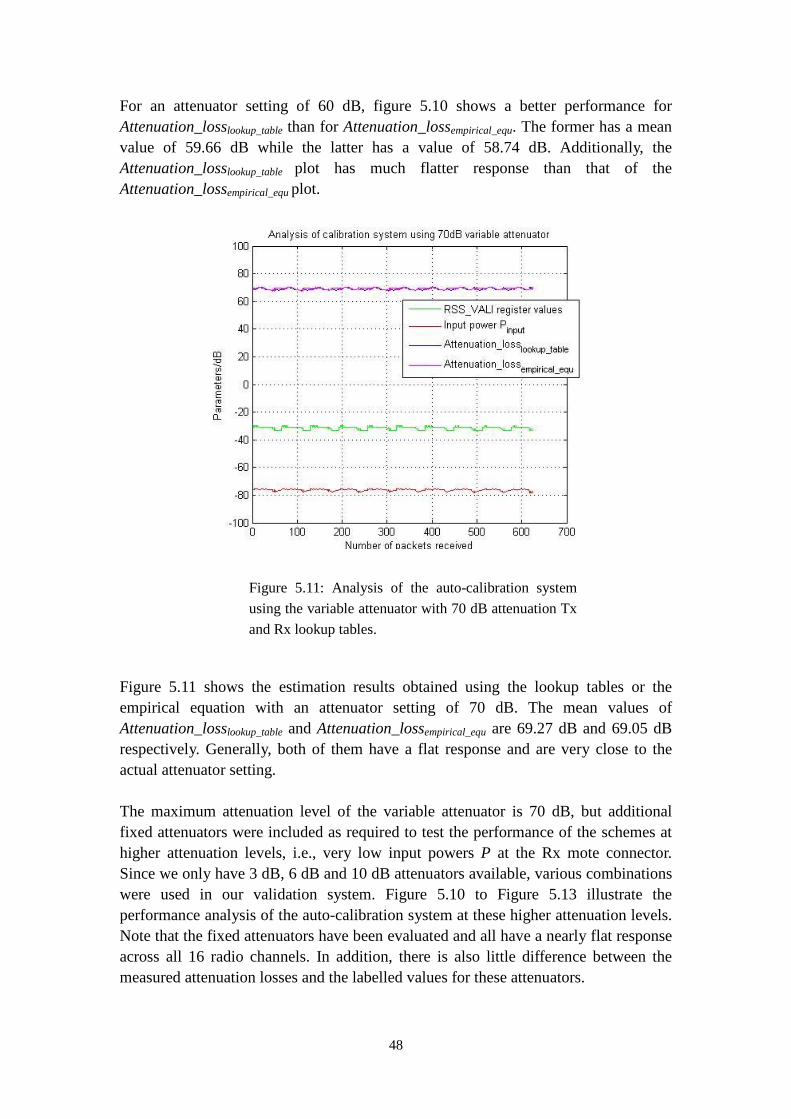
For an attenuator setting of 60 dB, figure 5.10 shows a better performance for Attenuation_losslookup_table than for Attenuation_lossempirical_equ. The former has a mean value of 59.66 dB while the latter has a value of 58.74 dB. Additionally, the Attenuation_losslookup_table plot has much flatter response than that of the Attenuation_lossempirical_equ plot.

Figure 5.11 shows the estimation results obtained using the lookup tables or the empirical equation with an attenuator setting of 70 dB. The mean values of Attenuation_losslookup_table and Attenuation_lossempirical_equ are 69.27 dB and 69.05 dB respectively. Generally, both of them have a flat response and are very close to the actual attenuator setting. The maximum attenuation level of the variable attenuator is 70 dB, but additional fixed attenuators were included as required to test the performance of the schemes at higher attenuation levels, i.e., very low input powers P at the Rx mote connector. Since we only have 3 dB, 6 dB and 10 dB attenuators available, various combinations were used in our validation system. Figure 5.10 to Figure 5.13 illustrate the performance analysis of the auto-calibration system at these higher attenuation levels. Note that the fixed attenuators have been evaluated and all have a nearly flat response across all 16 radio channels. In addition, there is also little difference between the measured attenuation losses and the labelled values for these attenuators.

Figure 5.11: Analysis of the auto-calibration system

using the variable attenuator with 70 dB attenuation Tx

and Rx lookup tables.

49

From Figure 5.12 it can be seen clearly that though the mean values given by Attenuation_losslookup_table and Attenuation_lossempirical_equ are about 79 dB, both exhibit quite large fluctuations. In addition, it should also be noted that some packets are being dropped at the receiving mote owing to low levels of received power. Figure 5.13 shows the performance with an 83 dB attenuation level. The mean values of Attenuation_losslookup_table and Attenuation_lossempirical_equ are approximately 81 dB and 82 dB respectively. The input power P is down to -88 dBm where even more received packets are lost compared with the previous case. This implies that Chipcon CC2420 transceiver is approaching its receiver sensitivity limit. The claimed receiver sensitivity is typically -95 dBm to -90 dBm [10].

Figure 5.12: Analysis of the auto-calibration system using the

attenuation of 79 dB. It consists of the variable attenuator of 70

dB, one 3 dB attenuator and one 6 dB attenuator.

50

Figure 5.14: Analysis of the auto-calibration system using

the attenuation of 86 dB. It consists of the variable

attenuator of 70 dB, one 6 dB attenuator and one 10 dB

attenuator.

Figure 5.13: Analysis of the auto-calibration system using the

attenuation of 83 dB. It consists of the variable attenuator of

70 dB, one 3 dB attenuator and one 10 dB attenuator.

51

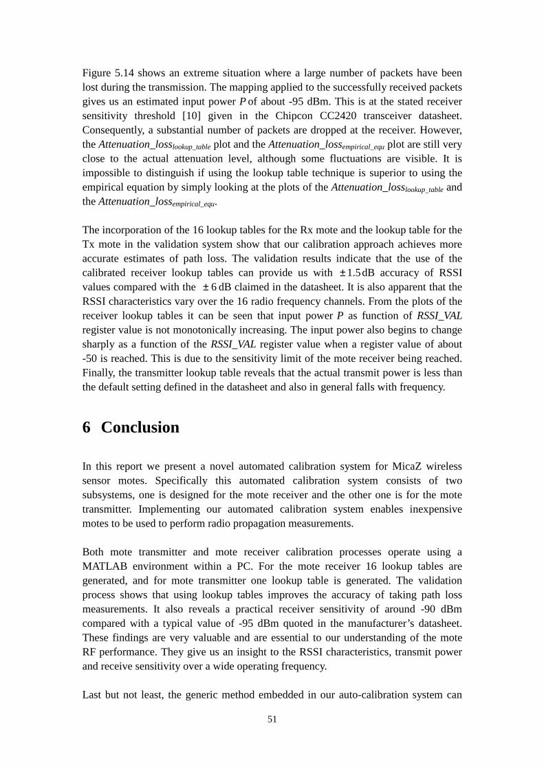
Figure 5.14 shows an extreme situation where a large number of packets have been lost during the transmission. The mapping applied to the successfully received packets gives us an estimated input power P of about -95 dBm. This is at the stated receiver sensitivity threshold [10] given in the Chipcon CC2420 transceiver datasheet. Consequently, a substantial number of packets are dropped at the receiver. However, the Attenuation_losslookup_table plot and the Attenuation_lossempirical_equ plot are still very close to the actual attenuation level, although some fluctuations are visible. It is impossible to distinguish if using the lookup table technique is superior to using the empirical equation by simply looking at the plots of the Attenuation_losslookup_table and the Attenuation_lossempirical_equ. The incorporation of the 16 lookup tables for the Rx mote and the lookup table for the Tx mote in the validation system show that our calibration approach achieves more accurate estimates of path loss. The validation results indicate that the use of the calibrated receiver lookup tables can provide us with 5.1± dB accuracy of RSSI values compared with the 6± dB claimed in the datasheet. It is also apparent that the RSSI characteristics vary over the 16 radio frequency channels. From the plots of the receiver lookup tables it can be seen that input power P as function of RSSI_VAL register value is not monotonically increasing. The input power also begins to change sharply as a function of the RSSI_VAL register value when a register value of about -50 is reached. This is due to the sensitivity limit of the mote receiver being reached. Finally, the transmitter lookup table reveals that the actual transmit power is less than the default setting defined in the datasheet and also in general falls with frequency.

6 Conclusion

In this report we present a novel automated calibration system for MicaZ wireless sensor motes. Specifically this automated calibration system consists of two subsystems, one is designed for the mote receiver and the other one is for the mote transmitter. Implementing our automated calibration system enables inexpensive motes to be used to perform radio propagation measurements. Both mote transmitter and mote receiver calibration processes operate using a MATLAB environment within a PC. For the mote receiver 16 lookup tables are generated, and for mote transmitter one lookup table is generated. The validation process shows that using lookup tables improves the accuracy of taking path loss measurements. It also reveals a practical receiver sensitivity of around -90 dBm compared with a typical value of -95 dBm quoted in the manufacturer’s datasheet. These findings are very valuable and are essential to our understanding of the mote RF performance. They give us an insight to the RSSI characteristics, transmit power and receive sensitivity over a wide operating frequency. Last but not least, the generic method embedded in our auto-calibration system can

52

also be easily applied to any other wireless sensor mote platforms from different vendors, provided they have an RF connector. In the future the research could be extended by investigating the possibility of reducing the time taken to perform the proposed automated calibration processes to enable mass calibration of wireless sensor motes. Moreover, we have shown that standard motes can be used as the low cost portable measurement equipment after going through the automated calibration process. For example the calibrated motes could be used to perform path loss measurements as a function of frequency in order to quantify the likely benefits of applying frequency diversity techniques.

53

References

[1] I. F. Akyildiz, W. Su, Y. Sankarasubramaniam, and E. Cayirci, “Wireless sensor networks: a survey," Computer Networks (Amsterdam, Netherlands: 1999), vol. 38, no. 4, pp. 393-422, 2002. [Online].Available: http://citeseer.ist.psu.edu/akyildiz02wireless.html

[2] K. Romer and F. Mattern, “The design space of wireless sensor networks," IEEE

Wireless Communications, vol. 11, no. 6, pp. 54-61, December 2004. [3] Technical overview of time synchronized mesh protocol (TSMP), Dust Networks,

2006. [Online]. Available: http://dustnetworks.com/docs/TSMP_Whitepaper.pdf [4] S. Saha and P. Bajcsy, “System design issues for applications using wireless

sensor networks," Automated Learning Group, National Centre for Supercomputing Applications, Tech. Rep. Technical Report alg03, August 2003.

[5] Y. Yao and J. Gehrke, “The cougar approach to in-network query processing in

sensor networks," 2002. [Online].Available: http://citeseer.ist.psu.edu/yao02cougar.html

[6] Crossbow Technology Inc. [Online]. Available: http://www.xbow.com [7] K. Whitehouse and D. Culler, “Calibration as parameter estimation in sensor

networks," in Proceedings of the 1st ACM international workshop on Wireless sensor networks and applications, pp. 59-67, 2002.

[8] B. Lau and M. Lyons, “Lazy calibration for wireless sensor networks," 2007. [9] MPR-MIB Users Manual, Crossbow Technology Inc. [Online]. Available:

http://www.xbow.com/Support/Support_pdf_files/MPR-MIB_Series_Users_Manual.pdf

[10] 2.4 GHz IEEE 802.15.4/ZigBee-ready RF Transceiver, CC2420 Data Sheet,

Chipcon AS. [Online]. Available: http://focus.ti.com/lit/ds/symlink/cc2420.pdf [11]J. Hill, R. Szewczyk, A. Woo, S. Hollar, D. E. Culler, and K. S. J. Pister. “System

Architecture Directions for Networks Sensors,” in Architecture Support for Programming Languages and Operating System, pp. 93-104, 2000.

[12] C. C. Han, R. K. Rengaswamy, R. Shea, E. Kohler, and M. Srivastava. “SOS: A

dynamic operating system for sensor networks,” in Proceedings of the Third

54

International Conference on Mobile Systems, Applications, and Services (Mobisys), 2005.

[13] H. Abrach, S. Bhatti, J. Carlson, H. Dai, J. Rose, A. Sheth, B. Shucker, J. Deng, and R. Han. “MANTIS: System support for multimodal NeTworks of in-situ sensors,” in Proceedings of the 2nd ACM international conference on Wireless Sensor Networks and Applications (WSNA), pp. 50-59, 2003.

[14] P. Levis, D. Gay, V. Handziski, J. H. Hauer, B. Greenstein, M. Turon, J. Hui, C.

Sharp, R. Szewczyk, and others. “T2: A second generation os for embedded sensor networks,” Telecommunication Networks Group, Technische Universitat Berlin, Tech. Rep. TKN-05-007, Nov, 2005.

[15] D. Gay, P. Levis, R. von Behren, M. Welsh, E. Brewer, and D. Culler. “The nesC

language: A holistic approach to networked embedded systems,” in Proceedings of Programming Language Design and Implementation (PLDI), June 2003.

[16] B. W. Kernighan and D. M. Ritchie. “The C Programming Language, Second

Edition,” Prentice Hall, 1988. [17] VPP-4.3: The VISA Library, IVI Foundation, 2008. [Online]. Available:

http://www.ivifoundation.org/docs/vpp43.pdf [18] IEEE std. 802.15.4 – 2003: Wireless Medium Access Control (MAC) and

Physical Layer (PHY) specifications for Low Rate Wireless Personal Area Networks (LR-WPANs). [Online]. Available: http://standards.ieee.org/getieee802/download/802.15.4-2003.pdf

[19] MS2721A Spectrum Analyzer Programming Manual, Anritsu Company. [Online].

Available: http://www.us.anritsu.com/downloads/files/10580-00104.pdf [20] Mini-Circuits: Power Splitter/Combiner: ZN2PD2-50-SMA, Mini-Circuits.

[Online]. Available: http://www.minicircuits.com/pdfs/ZN2PD2-50.pdf [21] Datasheet, Solewise Ltd. [Online]. Available: http://www.solewise.co.uk/

55

Appendix A

1 16 raw lookup tables for the Rx mote under test

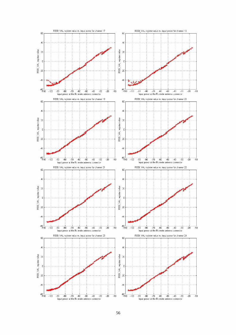
56

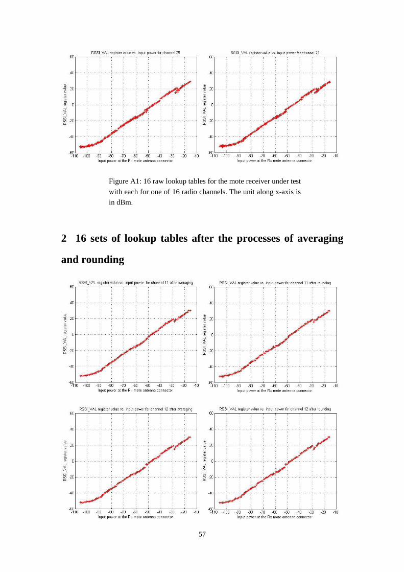
57

2 16 sets of lookup tables after the processes of averaging

and rounding

Figure A1: 16 raw lookup tables for the mote receiver under test

with each for one of 16 radio channels. The unit along x-axis is

in dBm.

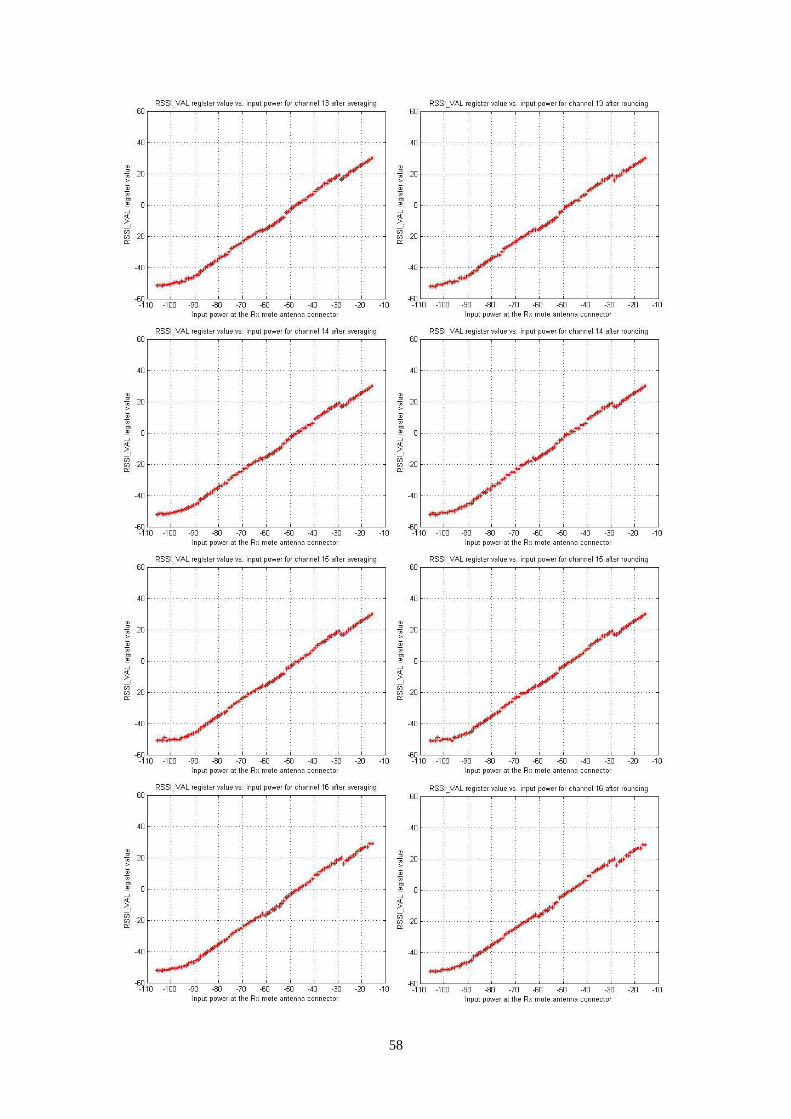
58

59

60

61

3 16 lookup tables after the process of deduplicating for the

Rx mote under test

Figure A2: 16 sets of lookup tables after the processes of averaging and rounding. The unit along x-axis is in dBm.

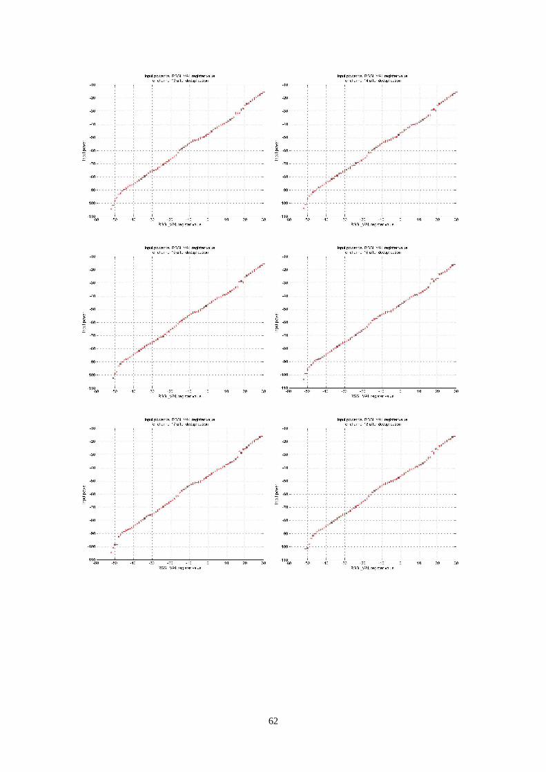
62

63

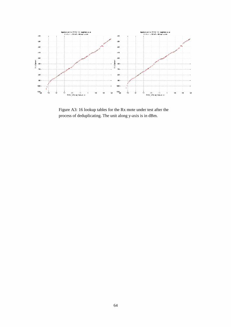
64

Figure A3: 16 lookup tables for the Rx mote under test after the

process of deduplicating. The unit along y-axis is in dBm.

65

Appendix B

1 Frequency response of Agilent-8495B manual step

attenuator

Measured attenuation on different radio Channels (dB) Attenuation

level (dB) 11 12 13 14 15 16 17 18

10 10.67 10.70 10.69 10.70 10.74 10.66 10.66 10.62

20 20.57 20.58 20.56 20.54 20.56 20.55 20.54 20.51

30 30.55 30.49 30.52 30.54 30.58 30.57 30.52 30.48

40 40.48 40.45 40.47 40.41 40.40 40.41 40.38 40.39

50 50.42 50.49 50.46 50.37 50.36 50.36 50.38 50.32

60 60.32 60.31 60.34 60.30 60.29 60.35 60.34 60.30

70 70.32 70.24 70.33 70.24 70.31 70.26 70.29 70.14

Measured attenuation on different radio Channels (dB) Attenuation

level (dB) 19 20 21 22 23 24 25 26

10 10.57 10.54 10.54 10.56 10.54 10.57 10.45 10.45

20 20.48 20.44 20.45 20.48 20.52 20.58 20.46 20.46

30 30.49 30.52 30.48 30.43 30.40 30.44 30.34 30.36

40 40.40 40.34 40.34 40.40 40.42 40.48 40.31 40.32

50 50.28 50.24 50.25 50.24 50.25 50.31 50.20 50.22

60 60.24 60.25 60.23 60.28 60.18 60.19 60.09 60.15

70 70.14 70.15 70.19 70.15 70.04 70.06 70.02 70.06

Table B1: Frequency response of Agilent-8945B manual step attenuator at the different attenuation level from 10 dB to 70 dB.