mtech adsa final 2nd jan 1,2,3,4

ADVANCED DATA STRUCTURES AND ALGORITHMS

SYLLABUS

UNIT I

Algorithms, Performance Analysis- Time Complexity And Space Complexity, Asymptotic Notation-Big Oh, Omega And Theta Notations, Complexity Analysis Examples. Data Structures-Linear And Non Linear Data Structures, Adt Concept, Linear List Adt, Array Representation, Linked Representation, Vector Representation, Singly Linked Lists -Insertion, Deletion, Search Operations, Doubly Linked Lists-Insertion, Deletion Operations, Circular Lists. Representation Of Single, Two Dimensional Arrays, Sparse Matrices And Their Representation.

UNIT II

Stack And Queue Adts, Array And Linked List Representations, Infix To Postfix Conversion Using Stack, Implementation Of Recursion, Circular Queue-Insertion And Deletion, Dequeue Adt, Array And Linked List Representations, Priority Queue Adt, Implementation Using Heaps, Insertion Into A Max Heap, Deletion From A Max Heap, Java.Util Package-Arraylist, Linked List, Vector Classes, Stacks And Queues In Java.Util, Iterators In Java.Util.

UNIT III

Searching–Linear And Binary Search Methods, Hashing-Hash Functions, Collision Resolution Methods-Open Addressing, Chaining, Hashing In Java.Util-Hashmap, Hashset, Hashtable. Sorting –Bubble Sort, Insertion Sort, Quick Sort, Merge Sort, Heap Sort, Radix Sort, Comparison Of Sorting Methods.

UNIT IV

Trees- Ordinary And Binary Trees Terminology, Properties Of Binary Trees, Binary Tree Adt, Representations, Recursive And Non Recursive Traversals, Java Code For Traversals, Threaded Binary Trees. Graphs- Graphs Terminology, Graph Adt, Representations, Graph Traversals/Search Methods-Dfs And Bfs, Java Code For Graph Traversals, Applications Of Graphs-Minimum Cost Spanning Tree Using Kruskal’s Algorithm, Dijkstra’s Algorithm For Single Source Shortest Path Problem.

UNIT V

Search Trees- Binary Search Tree-Binary Search Tree Adt, Insertion, Deletion And Searching Operations, Balanced Search Trees, Avl Trees-Definition And Examples Only, Red Black Trees – Definition And Examples Only, B-Trees-Definition, Insertion And Searching Operations, Trees In Java.Util- Treeset, Tree Map Classes, Tries(Examples Only),Comparison Of Search Trees. Text Compression-Huffman Coding And Decoding, Pattern Matching-Kmp Algorithm.

TEXTBOOK:

1. Data structures, Algorithms and Applications in Java, S.Sahni, Universities Press.

2. Data structures and Algorithms in Java, Adam Drozdek, 3rd edition, Cengage Learning.

3. Data structures and Algorithm Analysis in Java, M.A.Weiss, 2nd edition, Addison-Wesley (Pearson Education).

REFERENCES:

1. Java for Programmers, Deitel and Deitel, Pearson education.

N@ru Mtech Cse(1-1) Study Material (R13)

2. Data structures and Algorithms in Java, R.Lafore, Pearson education. 3. Java: The Complete Reference, 8th editon, Herbert Schildt, TMH. 4. Data structures and Algorithms in Java, M.T.Goodrich, R.Tomassia, 3rd edition,

Wiley India Edition. 5. Data structures and the Java Collection Frame work,W.J.Collins, Mc Graw Hill. 6. Classic Data structures in Java, T.Budd, Addison-Wesley (Pearson Education). 7. Data structures with Java, Ford and Topp, Pearson Education. 8. Data structures using Java, D.S.Malik and P.S.Nair, Cengage learning. 9. Data structures with Java, J.R.Hubbard and A.Huray, PHI Pvt. Ltd. 10. Data structures and Software Development in an Object-Oriented Domain,

J.P.Tremblay and G.A.Cheston, Java edition, Pearson Education.

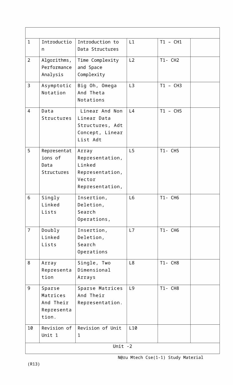
SESSION PLAN:

Sl.No.

Topic in Syllabus

Modules and Sub Modules

Lecture No. Suggested Books

Remarks

Unit -1

1 Introduction Introduction to Data Structures

L1 T1 – CH1

2 Algorithms, Performance Analysis

Time Complexity and Space Complexity

L2 T1- CH2

3 Asymptotic Notation

Big Oh, Omega And Theta Notations

L3 T1 – CH3

4 Data Structures

Linear And Non Linear Data Structures, Adt Concept, Linear List Adt

L4 T1 – CH5

5 Representations of Data Structures

Array Representation, Linked Representation, Vector Representation,

L5 T1- CH5

6 Singly Linked Lists

Insertion, Deletion, Search Operations,

L6 T1- CH6

7 Doubly Linked Lists

Insertion, Deletion, Search Operations

L7 T1- CH6

8 Array Representation

Single, Two Dimensional Arrays

L8 T1- CH8

9 Sparse Matrices And Their Representation.

Sparse Matrices And Their Representation.

L9 T1- CH8

10 Revision of Unit 1

Revision of Unit 1 L10


Unit -2

11 Stack Adt Insert, delete, search operations

L11 T1- CH9

12 Queue Adt Insert, delete, search operations

L12 T1- CH9

13 Representations of Stacks and Queues

Array And Linked List Representations

L13 T1- CH9

14 Conversions Infix To Postfix Conversion Using Stacks

L14 T1- CH9

15 Implementation Of Recursion

Implementation Of Recursion

L15 T2- CH5

16 Circular Queue Insertion And Deletion

L16 T2- CH5

17 Dequeue Adt Array And Linked List Representations

L17 T2- CH8

18 Priority Queue Adt

Implementation Using Heaps

L18 T1- CH13,T2-4

19 Heaps Insertion Into A Max Heap, Deletion From A Max Heap, Java.Util Package-Arraylist, Linked List, Vector Classes, Stacks And Queues In Java.Util, Iterators In Java.Util.

L19 T1- CH13



Unit – 3

21 Searching Linear And Binary Search Methods

L21 T2- CH3

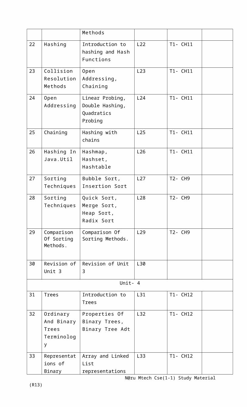
22 Hashing Introduction to hashing and Hash Functions

L22 T1- CH11

23 Collision Resolution Methods

Open Addressing, Chaining

L23 T1- CH11

24 Open Addressing

Linear Probing, Double Hashing, Quadratics Probing

L24 T1- CH11

25 Chaining Hashing with chains L25 T1- CH11

26 Hashing In Hashmap, Hashset, L26 T1- CH11


Java.Util Hashtable

27 Sorting Techniques

Bubble Sort, Insertion Sort

L27 T2- CH9

28 Sorting Techniques

Quick Sort, Merge Sort, Heap Sort, Radix Sort

L28 T2- CH9

29 Comparison Of Sorting Methods.

Comparison Of Sorting Methods.

L29 T2- CH9



Unit- 4

31 Trees Introduction to Trees L31 T1- CH12

32 Ordinary And Binary Trees Terminology

Properties Of Binary Trees, Binary Tree Adt

L32 T1- CH12

33 Representations of Binary Trees

Array and Linked List representations of Binary Trees

L33 T1- CH12

34 Traversals of Binary Trees

Recursive And Non Recursive Traversals

L34 T1- CH12

35 Java Code For Traversals

Java Code For Traversals

L35 T1- CH12

36 Threaded Binary Trees

Insert, search, Delete operations

L36 T1- CH12

37 Graph Adt, Representations

Graph Traversals L37 T1- CH17

38 Search Methods

Dfs And Bfs L38 T1- CH17

39 Java Code For Graph Traversals

Applications Of Graphs-Minimum Cost Spanning Tree Using Kruskal’s Algorithm, Dijkstra’s Algorithm For Single Source Shortest Path Problem.

L39 T1- CH17



Unit – 5

41 Search Trees Introduction to Binary Search Tree

L41 T1- CH15

42 Binary Search Tree Adt

Insertion, Deletion And Searching

L42 T1- CH15


Operations

43 Balanced Search Trees

Avl Trees-Definition And Examples

L43 T1- CH16

44 Red Black Trees

Definition And Examples

L44 T1- CH16

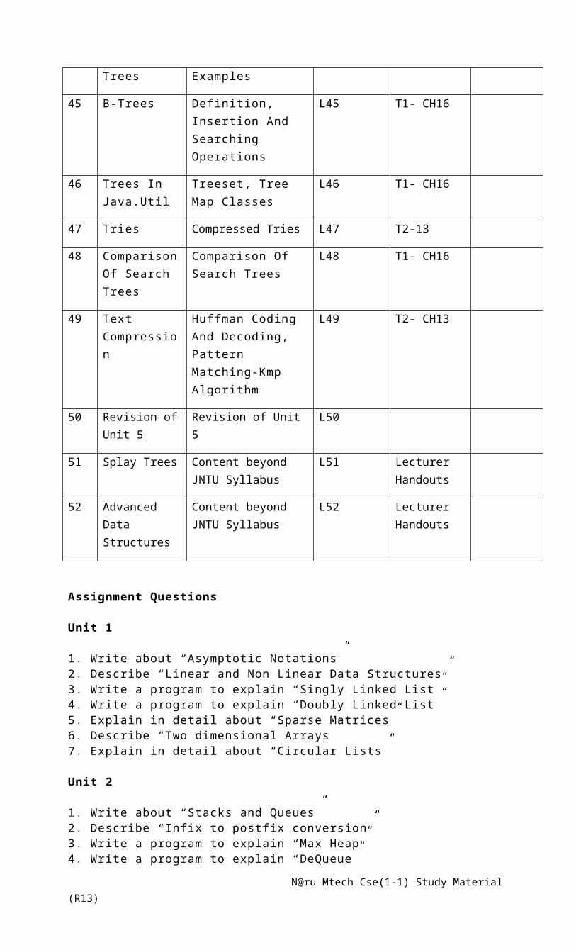
45 B-Trees Definition, Insertion And Searching Operations

L45 T1- CH16

46 Trees In Java.Util

Treeset, Tree Map Classes

L46 T1- CH16

47 Tries Compressed Tries L47 T2-13

48 Comparison Of Search Trees

Comparison Of Search Trees

L48 T1- CH16

49 Text Compression

Huffman Coding And Decoding, Pattern Matching-Kmp Algorithm

L49 T2- CH13



51 Splay Trees Content beyond JNTU Syllabus

L51 Lecturer Handouts

52 Advanced Data Structures

Content beyond JNTU Syllabus

L52 Lecturer Handouts

Assignment Questions

Unit 1

1. Write about “Asymptotic Notations”2. Describe “Linear and Non Linear Data Structures”3. Write a program to explain “Singly Linked List”4. Write a program to explain “Doubly Linked List”5. Explain in detail about “Sparse Matrices”6. Describe “Two dimensional Arrays”7. Explain in detail about “Circular Lists”

Unit 2

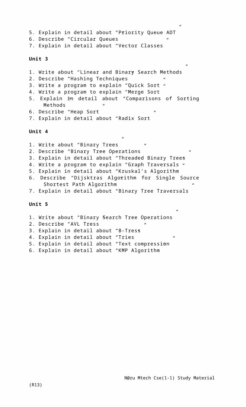
1. Write about “Stacks and Queues”2. Describe “Infix to postfix conversion”3. Write a program to explain “Max Heap”4. Write a program to explain “DeQueue”5. Explain in detail about “Priority Queue ADT”6. Describe “Circular Queues”7. Explain in detail about “Vector Classes”

Unit 3

1. Write about “Linear and Binary Search Methods”


2. Describe “Hashing Techniques”3. Write a program to explain “Quick Sort”4. Write a program to explain “Merge Sort”5. Explain in detail about “Comparisons of Sorting Methods”6. Describe “Heap Sort”7. Explain in detail about “Radix Sort”

Unit 4

1. Write about “Binary Trees”2. Describe “Binary Tree Operations”3. Explain in detail about “Threaded Binary Trees”4. Write a program to explain “Graph Traversals”5. Explain in detail about “Kruskal’s Algorithm”6. Describe “Dijsktras Algorithm for Single Source Shortest Path

Algorithm”7. Explain in detail about “Binary Tree Traversals”

Unit 5

1. Write about “Binary Search Tree Operations”2. Describe “AVL Tress”3. Explain in detail about “B-Tress”4. Explain in detail about “Tries”5. Explain in detail about “Text compression”6. Explain in detail about “KMP Algorithm”

UNIT – 1

Contents:

1. Explain in detail about an “Algorithm”

An algorithm is a finite set of instructions that is followed accomplishes a particular task. (or) an algorithm is a step-by-step process of solving a particular problem. The algorithm must satisfy the following criteria.

Input: zero ore more quantities are exactly supplied.

Output: At least one quantity is produced.

Definiteness: Each instruction is clear and unambiguous.

Finiteness: The algorithm should be finite that means after a finite number of steps it should


terminate.

Effectiveness: Every step of the algorithm should be feasible.

Ex: algorithm to count the sum of n numbers

Algorithm sum (1,n)

{

Result:=0;

For i:=1 to n do i:=i+1;

result:=result + i;

}

2. Describe Performance Analysis in detail?

The efficiency of an algorithm can be decided by measuring the performance of an algorithm. We can measure the performance of an algorithm by computing the amount of time and storage requirement.

2.1 Space Complexity:

The space complexity can be defined as amount of memory required by an algorithm to run.

To compute the space complexity we use two factors: constant and instance characteristic. The space requirement s(p) can be given as

S(p)= c + sp

Where c is constant i.e., fixed part and it denotes the space of inputs and outputs. This space is an amount of memory space taken by instruction, variable and identifiers.

The term Space Complexity is misused for Auxiliary Space at many places.

Auxiliary Space is the extra space or temporary space used by an algorithm.

Space Complexity of an algorithm is total space taken by the algorithm with respect to the input size. Space complexity includes both Auxiliary space and space used by input.

For example, if we want to compare standard sorting algorithms on the basis of space, then Auxiliary Space would be better criteria than Space Complexity. Merge Sort uses O(n) auxiliary space, Insertion sort and Heap Sort use O(1) auxiliary space. Space complexity of all these sorting algorithms is O(n)

Space complexity is a measure of the amount of working storage an algorithm needs. That means how much memory, in the worst case, is needed at any point in the algorithm. As with time complexity, we're mostly concerned with how the space needs grow, in big-Oh terms, as the size N of the input problem grows.

For example,

int sum(int x, int y, int z) { int r = x + y + z; return r;}

requires 3 units of space for the parameters and 1 for the local variable, and this never changes, so this is O(1).


int sum(int a[], int n) { int r = 0; for (int i = 0; i < n; ++i) { r += a[i]; } return r;}

requires n units for a, plus space for n, r and i, so it's O(n)

2.2 Time Complexity:

The time complexity of an algorithm is the amount of computer time required by analgorithm to run to completion.

There are two types of computing time- compile time and rum time. The timecomplexity is generally computed using run time or execution time.

It is difficult to compute the time complexity in terms of physically clocked time. Forinstance in multiuser system, executing time depends on many factors such as systemload, number of other programs running, instruction set used.

The time complexity is therefore given in terms of frequency count.

Frequency count is basically a count denoting number of times of execution ofstatement.

Ex:

Algorithm sum(A,B,C,m,n) frequency total

{ - -

For i:= 1 to m do m+1 m+1

For j:= 1 to n do m(n+1) m(n+1)

C[i,j]:= A[I,j] –B[ i,j]; mn mn

} - -

2mn+2m+1

So the time complexity of above algorithm is ‘mn’ by neglecting the constants.

3) Explain in detail about “Asymptotic Notations”?

Measuring Efficiency is depend upon the following

When algorithm is applied to a large data set, will finish relatively quickly. Speed and memory usage

Measuring speed-we measure algorithm speed in terms of Operations relative to input size.

Big O Notation

Definition: Let f(x) and g(x) be two functions; We say thatf(x) O(g(x))

if there exists a constant c, Xo > 0 such that f(x)≤c*g(x) for all X ≥ Xo.

f (x) is asymptotically less than or equal to g(x)

Big-O gives an asymptotic upper bound.


C*g(x)

g(x)f(x)

x

y

xo

Big-Omega Notation:

Definition: Letf (x)andg(x) be two functions; We say thatf(x) (g(x))

if there exists a constant c, Xo ≥ 0such that f(x) ≥ c*g(x) for all X ≥ Xo

f(x) is asymptotically greater than or equal to g(x)

Big-Omega gives an asymptotic lower bound


C*g(x)

g(x)f(x)

x

y

xo

Big Θ Notation:

Definition: Let f(x) and g(x) be two functions ; We say thatf(x) (g(x)) if there exists a constant c1, c2, Xo > 0; such that for every integer x x0 we have c1g(x) ≥ f(x) ≥ c2g(x)

F(x) is asymptotically equal to g(x)

F(x) is bounded above and below by g(x)

Big-Theta gives an asymptotic equivalence

4) Illustrate ‘Linear and nonlinear data structures’ in brief?

Data structure is a systematic way of organizing and accessing data. There are two types of Non-Primitive Data Structures. They are,

Linear data structures are lists, stacks and queues Non-Linear data structures are trees and graphs

List ADT

List is a collection of elements arranged in sequential manner. Hence a list is a sequence of zero

or more elements of given type, the form of list is

a1, a2, a3, a4 ,……………………..an (n>=0)

where

n - Number of elements in the list

a1 - First element in the list

an- Last element in the list

Lists can be represented in two ways:

Elements stored with arrays

Elements stored with pointers

List is an abstract data type that includes a finite set of items.

4.1 Operations:


C2*g(x)

g(x)f(x)

x

y

xo

C1*g(x)

empty () - returns true if the list is empty, otherwise false

size() - returns the size of the list

get(index) - returns the index of the first occurrence of ‘x’ in the list, returns ‘-1’

if ‘x’ not in the list

erase(index) - delete the element based on the given index. Elements with higher

index have their index reduced by 1.

insert(index, x) - insert ‘x’ at the given index, elements with the index >= index

have their index increased by 1.

output() - output the list elements from the left to right.

We know that in the array implementation of lists, the sequential organization is provided

implicitly by its index. We use the index for accessing and manipulation of array elements.

One major problem with the arrays is that size of an array must be specified precisely

at the beginning. This may be difficult task in many practical applications. Other problems

are due to the difficulty in insertion and deletion at the beginning of the array since it takes

time O(n).

A completely different way to represent a list is to make each item in the list part of a

structure that also contains a ‘link’ to the structure containing the next item as shown in the

following fig, this type of list is called a linked list, because it is a list whose order is given by

links from one to the next.

Types of Linked Lists:

Basically there are four types of linked list single linked list doubly linked list circular linked list circular – doubly linked list

Single Linked List: the simplest kind of linked list is a single –linked list, which hasone link per

node. This link points to the next node in the list or to a null value if it is the finalnode.

Doubly Linked List: a more sophisticated kind of linked list is a doubly linked list or

two way linked list. Each node has two links:

One of them points to previous node or points to a null value if it is the first node.

The other points to the next node or points to a null value if it is a final node.

Circular Linked List: in this, the first and the final nodes are linked together. In fact in

a singly circular linked list each node has one link. Similarly, to an ordinary singly linked list,

except that the next link of the last node points to the first node.

Circular Doubly Linked List: in this, each mode has two links, similarly to doubly

linked list, except that the previous link of the first node points to the last node and the next


link of the last node points to the first node.

Advantages: Memory is allocated dynamically. Insertion and deletion is easy. Data is deleted physically.

5) Explain in detail about “Representations of Linear List with a program”?

A list or sequence is an abstract data type that implements a finite ordered collection of values, where the same value may occur more than once. An instance of a list is a computer representation of the mathematical concept of a finite sequence; the (potentially) infinite analog of a list is a stream. Lists are a basic example of containers, as they contain other values. Each instance of a value in the list is usually called an item, entry, or element of the list; if the same value occurs multiple times, each occurrence is considered a distinct item. Lists are distinguished from arrays in that lists only allow sequential access, while arrays allow random access.

The name list is also used for several concrete data structures that can be used to implement abstract lists, especially linked lists.

The so-called static list structures allow only inspection and enumeration of the values. A mutable or dynamic list may allow items to be inserted, replaced, or deleted during the list's existence.

Linear List Array Representation

Use a one-dimensional array element[]

L = (a, b, c, d, e)

Store element i of list in element[i].

A java Program for Array Representation of Linear List

A List Interfacepublic interface List { public void createList(int n); public void insertFirst(Object ob); public void insertAfterbjectob, Object pos); (O public Object deleteFirst(); public Object deleteAfter(Object pos); publicbooleanisEmpty(); publicintsize(); }An ArrayListClassclassArrayListimplements List { classNode { Object data; int next;


http://en.wikipedia.org/wiki/Mutable_object

http://en.wikipedia.org/wiki/Linked_list

http://en.wikipedia.org/wiki/Data_structures

http://en.wikipedia.org/wiki/Random_access

http://en.wikipedia.org/wiki/Array_data_type

http://en.wikipedia.org/wiki/Container_(abstract_data_type)

http://en.wikipedia.org/wiki/Stream_(type_theory)

http://en.wikipedia.org/wiki/Sequence_(mathematics)

http://en.wikipedia.org/wiki/Mathematics

http://en.wikipedia.org/wiki/Value_(computer_science)

http://en.wikipedia.org/wiki/Abstract_data_type

Node(Object ob, inti) // constructor { data = ob; next = i; } } int MAXSIZE; // max number of nodes in the list Node list[]; // create list array int head, count; // count: current number of nodes in the list ArrayList(int s) // constructor { MAXSIZE = s; list = new Node[MAXSIZE]; }

public void initializeList() { for( int p = 0; p < MAXSIZE-1; p++ ) list[p] = new Node(null, p+1); list[MAXSIZE-1] = new Node(null, -1); } public void createList(int n) // create ‘n’ nodes { int p; for( p = 0; p < n; p++ ) { list[p] = new Node(11+11*p, p+1); count++; } list[p-1].next = -1; // end of the list } public void insertFirst(Object item) { if( count == MAXSIZE ) { System.out.println("***List is FULL"); return; } int p = getNode(); if( p != -1 ) { list[p].data = item; if(isEmpty() ) list[p].next = -1; else list[p].next = head; head = p; count++; } } public void insertAfter(Object item, Object x) { if( count == MAXSIZE ) { System.out.println("***List is FULL"); return; } int q = getNode(); // get the available position to insert new node int p = find(x); // get the index (position) of the Object x if( q != -1 ) { list[q].data = item; list[q].next = list[p].next; list[p].next = q;count++; } } publicintgetNode() // returns available node index { for( int p = 0; p < MAXSIZE; p++ ) if(list[p].data == null) return p; return -1; }


publicintfind(Object ob) // find the index (position) of the Object ob{ int p = head; while( p != -1) { if( list[p].data == ob ) return p; p = list[p].next; // advance to next node } return -1; } public Object deleteFirst() { if( isEmpty() ) { System.out.println("List is empty: no deletion"); return null; } Object tmp = list[head].data; if( list[head].next == -1 ) // if the list contains one node, head = -1; // make list empty. elsehead = list[head].next; count--; // update count returntmp; } public Object deleteAfter(Object x) { int p = find(x); if( p == -1 || list[p].next == -1 ) { System.out.println("No deletion"); return null; } int q = list[p].next; Object tmp = list[q].data; list[p].next = list[q].next; count--; returntmp; } public void display() { int p = head; System.out.print("\nList: [ " ); while( p != -1) { System.out.print(list[p].data + " "); // print data p = list[p].next; // advance to next node } System.out.println("]\n");// } publicbooleanisEmpty() { if(count == 0) return true; else return false; }publicintsize() { return count; } }Testing ArrayListClass

classArrayListDemo{ public static void main(String[] args) { ArrayListlinkedList = new ArrayList(10); linkedList.initializeList(); linkedList.createList(4); // create 4 nodes linkedList.display(); // print the list System.out.print("InsertFirst 55:"); linkedList.insertFirst(55); linkedList.display();


System.out.print("Insert 66 after 33:"); linkedList.insertAfter(66, 33); // insert 66 after 33 linkedList.display(); Object item = linkedList.deleteFirst(); System.out.println("Deleted node: " + item);

linkedList.display(); System.out.print("InsertFirst 77:"); linkedList.insertFirst(77); linkedList.display(); item = linkedList.deleteAfter(22); // delete node after node 22 System.out.println("Deleted node: " + item); linkedList.display(); System.out.println("size(): " + linkedList.size()); } }

b) Linked Representation

Let L = (e1,e2,…,en)– Each element ei is represented in a separate node– Each node has exactly one link field that is used to locate the next element in the

linear list– The last node, en, has no node to link to and so its link field is NULL.

This structure is also called a chain.

A LinkedListClass

classLinkedListimplements List { classNode { Object data; // data item Node next; // refers to next node in the list Node( Object d ) // constructor { data = d; } // ‘next’ is automatically set to null } Node head; // head refers to first node Node p; // p refers to current node int count; // current number of nodes public void createList(int n) // create 'n' nodes { p = new Node(11); // create first node head = p; // assign mem. address of 'p' to 'head' for(inti = 1; i< n; i++ ) // create 'n-1' nodes p = p.next = new Node(11 + 11*i); count = n; } public void insertFirst(Object item) // insert at the beginning of list { p = new Node(item); // create new node p.next = head; // new node refers to old head head = p; // new head refers to new node count++; }


public void insertAfter(Object item,Object key) { p = find(key); // get “location of key item” if( p == null ) System.out.println(key + " key is not found"); else{ Node q = new Node(item); // create new node q.next = p.next; // new node next refers to p.nextp.next = q; // p.next refers to new node count++; } } public Node find(Object key) { p = head; while( p != null ) // start at beginning of list until end of list { if(p.data == key ) return p; // if found, return key addressp = p.next; // move to next node } return null; // if key search is unsuccessful, return null } public Object deleteFirst() // delete first node { if(isEmpty() ) { System.out.println("List is empty: no deletion"); return null; }

Node tmp = head; // tmpsaves reference to head head = tmp.next; count--; returntmp.data; }

public Object deleteAfter(Object key) // delete node after key item { p = find(key); // p = “location of key node” if( p == null ) { System.out.println(key + " key is not found"); return null; } if(p.next == null ) // if(there is no node after key node) { System.out.println("No deletion"); return null; } else{ Nodetmp = p.next; // save node after key node p.next = tmp.next; // point to next of node deleted count--; returntmp.data; // return deleted node } } public void displayList() { p = head; // assign mem. address of 'head' to 'p' System.out.print("\nLinked List: "); while( p != null ) // start at beginning of list until end of list { System.out.print(p.data + " -> "); // print data p = p.next; // move to next node } System.out.println(p); // prints 'null' }

publicbooleanisEmpty() // true if list is empty { return (head == null); }


publicint size() { return count; } } // end of LinkeList class

Testing LinkedListClassclassLinkedListDemo{ public static void main(String[] args) { LinkedList list = new LinkedList(); // create list object

list.createList(4); // create 4 nodes list.displayList(); list.insertFirst(55); // insert 55 as first node list.displayList();

list.insertAfter(66, 33); // insert 66 after 33 list.displayList(); Object item = list.deleteFirst(); // delete first node if( item != null ) { System.out.println("deleteFirst(): " + item); list.displayList(); } item = list.deleteAfter(22); // delete a node after node(22) if( item != null ) { System.out.println("deleteAfter(22): " + item); list.displayList(); } System.out.println("size(): " + list.size()); } }

6) Explain in detail about “Single Linked List” with a java program?

The simplest kind of linked list is a single –linked list, which has one link per node. This link

points to the next node in the list or to a null value if it is the final node.

A linked list is a data structure consisting of a group of nodes which together represent a

sequence. Under the simplest form, each node is composed of a datum and a reference (in other

words, a link) to the next node in the sequence; more complex variants add additional links. This

structure allows for efficient insertion or removal of elements from any position in the sequence.

Linked lists are among the simplest and most common data structures. They can be used to implement several other common abstract data types, including lists (the abstract data type), stacks, queues, associative arrays, and S-expressions, though it is not uncommon to implement the other data structures directly without using a list as the basis of implementation.

The principal benefit of a linked list over a conventional array is that the list elements can easily be inserted or removed without reallocation or reorganization of the entire structure because the data items need not be stored contiguously in memory or on disk. Linked lists allow insertion and removal of nodes at any point in the list, and can do so with a constant number of operations if the link previous to the link being added or removed is maintained during list traversal.

On the other hand, simple linked lists by themselves do not allow random access to the data, or any form of efficient indexing. Thus, many basic operations — such as obtaining the last node of the list (assuming that the last node is not maintained as separate node reference in the list


http://en.wikipedia.org/wiki/Random_access

http://en.wikipedia.org/wiki/Array_data_structure

http://en.wikipedia.org/wiki/S-expression

http://en.wikipedia.org/wiki/Associative_array

http://en.wikipedia.org/wiki/Queue_(abstract_data_type)

http://en.wikipedia.org/wiki/Stack_(abstract_data_type)

http://en.wikipedia.org/wiki/List_(abstract_data_type)

http://en.wikipedia.org/wiki/Abstract_data_type

http://en.wikipedia.org/wiki/Reference_(computer_science)

http://en.wikipedia.org/wiki/Node_(computer_science)

http://en.wikipedia.org/wiki/Data_structure

structure), or finding a node that contains a given datum, or locating the place where a new node should be inserted — may require scanning most or all of the list elements.

Program:

import java.lang.*;import java.util.*;

public class Node{ Node data; node next;}

public class SinglyLinkeList{ Node start; int size;

public SinnglyLinkedList(){ start=null; size=0;}

public void add(Node data){ if(size=0) { start=new Node(); start.next=null; start.data=data; } else { Node currentnode=getnode(size-1); Node newnode=new Node(); newnode.data=data; newnode.next=null; currentnode.next=newnode; } size++; }

public void insertfront(Node data) { if(size==0) { Node newnode=new Node(); start.next=null; start.data=data; } else {


Node newnode=new Node(); newnode.data=data; newnode.next=start; } size++; }

public void insertAt(int position,Node data) { if(position==0) { insertatfront(Node data); } else if(position==size-1) { insertatlast(data); } else { Node tempnode=getNodeAt(position-1); Node newnode= new Node(); newnode.data=data; newnode.next=tempnode.next; size++; } }

public Node getFirst() { return getNodeAt(0); } public Node getLast() { return getNodeAt(size-1); } public Node removeAtFirst() { if(size==0) { System.out.println("Empty List "); } else { Node tempnode=getNodeAt(position-1); Node data=tempnode.next.data; tempnode.next=tempnode.next.next; size--; return data; } }

Node data=start.data; start=start.next; size--;


return data; } } public Node removeAtLast() { if(size==0) { System.out.println("Empty List "); } else { Node data=getNodeAt(size-1); Node data=tempnode.next.data; size--; return data; }}

public string void main(string[] args) {

LinkedList l1=new LinkedList(); BufferReader bf=new BufferReader(new InputStreamReader(Sysyem.in)); System.out.println("1->Add Element 2->Remove Last 3->Insert Front 4->Insert at position 5->REmove Front 6-> Remove At Last 7->Exit ");

string choice;choice.readline();int choiceNum= Integer.parseInt(choice);string str;switch(choiceNum){ case 1: System.out.println("Enter the element to be inserted "); str =bf.readline(); l1.add(str); break;

case 2: System.out.println("Linked List before removing element : "+l1); System.out.println("Linked List after removing element : "); l1.removeLast(); break;

case 3: System.out.println("Linked List before inserting element at first: "+l1); System.out.println("Enter the element to be inserted at first: "); str.readline(); l1.insertfront(str); System.out.println("Linked List after inserting at first : "+l1); break;

case 4: System.out.println("Linked List before inserting element at particular position: "+l1); System.out.println("Enter the element position & element : "); str.readline(); string str1; str1.readline(); l1.insertAt(str,str1); System.out.println("Linked List after inserting at particular Position :"+l1); break;

case 5: System.out.println("Linked LIst before removing front element: "+l1);


System.out.println("Linked List after removing front element : "); l1.removeAtFirst(); break;

case 6: System.out.println("Linked List before removing last element: "+l1); System.out.println("Linked List after removing last element :"); l1.removeAtLast();

default:break; } } }

7) Explain in detail about “Double Linked List” with a java program?

A more sophisticated kind of linked list is a doubly linked list or two way linked list. Each node

has two links:

One of them points to previous node or points to a null value if it is the first node.

The other points to the next node or points to a null value if it is a final node.

a doubly-linked list is a linked data structure that consists of a set of sequentially linked records called nodes. Each node contains two fields, called links, that are references to the previous and to the next node in the sequence of nodes. The beginning and ending nodes' previous and next links, respectively, point to some kind of terminator, typically a sentinel node or null, to facilitate traversal of the list. If there is only one sentinel node, then the list is circularly linked via the sentinel node. It can be conceptualized as two singly linked lists formed from the same data items, but in opposite sequential orders.

The two node links allow traversal of the list in either direction. While adding or removing a node in a doubly-linked list requires changing more links than the same operations on a singly linked list, the operations are simpler and potentially more efficient (for nodes other than first nodes) because there is no need to keep track of the previous node during traversal or no need to traverse the list to find the previous node, so that its link can be modified.

Program:

class Link { public long dData; // data item public Link next; // next link in list public Link previous; // previous link in list// ------------------------------------------------------------- public Link(long d) // constructor { dData = d; }// ------------------------------------------------------------- public void displayLink() // display this link { System.out.print(dData + " "); }// ------------------------------------------------------------- } // end class Link

class DoublyLinkedList


http://en.wikipedia.org/wiki/Linked_list

http://en.wikipedia.org/wiki/Null_pointer

http://en.wikipedia.org/wiki/Sentinel_node

http://en.wikipedia.org/wiki/Reference_(computer_science)

http://en.wikipedia.org/wiki/Field_(computer_science)


http://en.wikipedia.org/wiki/Record_(computer_science)

http://en.wikipedia.org/wiki/Linked_data_structure

{ private Link first; // ref to first item private Link last; // ref to last item// ------------------------------------------------------------- public DoublyLinkedList() // constructor { first = null; // no items on list yet last = null; }// ------------------------------------------------------------- public boolean isEmpty() // true if no links { return first==null; }// ------------------------------------------------------------- public void insertFirst(long dd) // insert at front of list { Link newLink = new Link(dd); // make new link

if( isEmpty() ) // if empty list, last = newLink; // newLink <-- last else first.previous = newLink; // newLink <-- old first newLink.next = first; // newLink --> old first first = newLink; // first --> newLink }// ------------------------------------------------------------- public void insertLast(long dd) // insert at end of list { Link newLink = new Link(dd); // make new link if( isEmpty() ) // if empty list, first = newLink; // first --> newLink else { last.next = newLink; // old last --> newLink newLink.previous = last; // old last <-- newLink } last = newLink; // newLink <-- last }// ------------------------------------------------------------- public Link deleteFirst() // delete first link { // (assumes non-empty list) Link temp = first; if(first.next == null) // if only one item last = null; // null <-- last else first.next.previous = null; // null <-- old next first = first.next; // first --> old next return temp; }// ------------------------------------------------------------- public Link deleteLast() // delete last link { // (assumes non-empty list) Link temp = last; if(first.next == null) // if only one item first = null; // first --> null


else last.previous.next = null; // old previous --> null last = last.previous; // old previous <-- last return temp; }// ------------------------------------------------------------- // insert dd just after key public boolean insertAfter(long key, long dd) { // (assumes non-empty list) Link current = first; // start at beginning while(current.dData != key) // until match is found, { current = current.next; // move to next link if(current == null) return false; // didn't find it } Link newLink = new Link(dd); // make new link

if(current==last) // if last link, { newLink.next = null; // newLink --> null last = newLink; // newLink <-- last } else // not last link, { newLink.next = current.next; // newLink --> old next // newLink <-- old next current.next.previous = newLink; } newLink.previous = current; // old current <-- newLink current.next = newLink; // old current --> newLink return true; // found it, did insertion }// ------------------------------------------------------------- public Link deleteKey(long key) // delete item w/ given key { // (assumes non-empty list) Link current = first; // start at beginning while(current.dData != key) // until match is found, { current = current.next; // move to next link if(current == null) return null; // didn't find it } if(current==first) // found it; first item? first = current.next; // first --> old next else // not first // old previous --> old next current.previous.next = current.next;

if(current==last) // last item? last = current.previous; // old previous <-- last else // not last // old previous <-- old next current.next.previous = current.previous;


return current; // return value }// ------------------------------------------------------------- public void displayForward() { System.out.print("List (first-->last): "); Link current = first; // start at beginning while(current != null) // until end of list, { current.displayLink(); // display data current = current.next; // move to next link } System.out.println(""); }// ------------------------------------------------------------- public void displayBackward() { System.out.print("List (last-->first): "); Link current = last; // start at end while(current != null) // until start of list, { current.displayLink(); // display data current = current.previous; // move to previous link } System.out.println(""); }// ------------------------------------------------------------- } // end class DoublyLinkedList

class DoublyLinkedApp { public static void main(String[] args) { // make a new list DoublyLinkedList theList = new DoublyLinkedList();

theList.insertFirst(22); // insert at front theList.insertFirst(44); theList.insertFirst(66);

theList.insertLast(11); // insert at rear theList.insertLast(33); theList.insertLast(55);

theList.displayForward(); // display list forward theList.displayBackward(); // display list backward

theList.deleteFirst(); // delete first item theList.deleteLast(); // delete last item theList.deleteKey(11); // delete item with key 11

theList.displayForward(); // display list forward

theList.insertAfter(22, 77); // insert 77 after 22 theList.insertAfter(33, 88); // insert 88 after 33


theList.displayForward(); // display list forward } // end main() } // end class DoublyLinkedApp

7) Explain in detail about “Circular List”?

Circular list

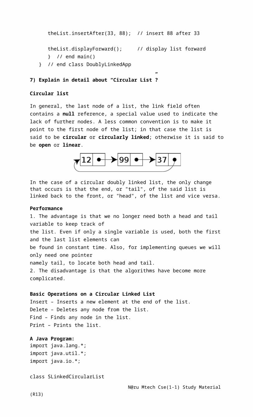
In general, the last node of a list, the link field often contains a null reference, a special value used to indicate the lack of further nodes. A less common convention is to make it point to the first node of the list; in that case the list is said to be circular or circularly linked; otherwise it is said to be open or linear.

In the case of a circular doubly linked list, the only change that occurs is that the end, or "tail", of the said list is linked back to the front, or "head", of the list and vice versa.

Performance1. The advantage is that we no longer need both a head and tail variable to keep track ofthe list. Even if only a single variable is used, both the first and the last list elements canbe found in constant time. Also, for implementing queues we will only need one pointernamely tail, to locate both head and tail.2. The disadvantage is that the algorithms have become more complicated.

Basic Operations on a Circular Linked ListInsert – Inserts a new element at the end of the list.Delete – Deletes any node from the list.Find – Finds any node in the list.Print – Prints the list.

A Java Program:import java.lang.*;import java.util.*;import java.io.*; class SLinkedCircularList{ private int data; private SLinkedCircularList next; public SLinkedCircularList() { data = 0; next = this; } public SLinkedCircularList(int value) { data = value; next = this; }



public SLinkedCircularList InsertNext(int value) { SLinkedCircularList node = new SLinkedCircularList(value); if (this.next == this) // only one node in the circular list { // Easy to handle, after the two lines of executions, // there will be two nodes in the circular list node.next = this; this.next = node; } else { // Insert in the middle SLinkedCircularList temp = this.next; node.next = temp; this.next = node; } return node; } public int DeleteNext() { if (this.next == this) { System.out.println("\nThe node can not be deleted as there is only one node in the circular list"); return 0; } SLinkedCircularList node = this.next; this.next = this.next.next; node = null; return 1; } public void Traverse() { Traverse(this); } public void Traverse(SLinkedCircularList node) { if (node == null) node = this; System.out.println("\n\nTraversing in Forward Direction\n\n"); SLinkedCircularList startnode = node; do { System.out.println(node.data); node = node.next;


} while (node != startnode); } public int GetNumberOfNodes() { return GetNumberOfNodes(this); } public int GetNumberOfNodes(SLinkedCircularList node) { if (node == null) node = this; int count = 0; SLinkedCircularList startnode = node; do { count++; node = node.next; } while (node != startnode); System.out.println("\nCurrent Node Value: " + node.data); System.out.println("\nTotal nodes in Circular List: " + count); return count; } public static void main(String[] args) { SLinkedCircularList node1 = new SLinkedCircularList(1); node1.DeleteNext(); // Delete will fail in this case. SLinkedCircularList node2 = node1.InsertNext(2); node1.DeleteNext(); // It will delete the node2. node2 = node1.InsertNext(2); // Insert it again SLinkedCircularList node3 = node2.InsertNext(3); SLinkedCircularList node4 = node3.InsertNext(4); SLinkedCircularList node5 = node4.InsertNext(5); node1.GetNumberOfNodes(); node3.GetNumberOfNodes(); node5.GetNumberOfNodes(); node1.Traverse(); node3.DeleteNext(); // delete the node "4" node2.Traverse(); node1.GetNumberOfNodes(); node3.GetNumberOfNodes();


node5.GetNumberOfNodes(); }}

8) Explain in detail about “Sparse Matrices”?

Data structures used to maintain sparse matrices must provide access to the nonzero elements of a matrix in a manner which facilitates efficient implementation of the algorithms that are examined in Section 8. The current sparse matrix implementation also seeks to support a high degree of generality both in problem size and the definition of a matrix element. Among other things, this implies that the algorithms must be able to solve problems that are too large to fit into core.

Simply put, the fundamental sparse matrix data structure is: Each matrix is a relation in a data base, and Each nonzero element of a matrix is a tuple in a matrix relation.

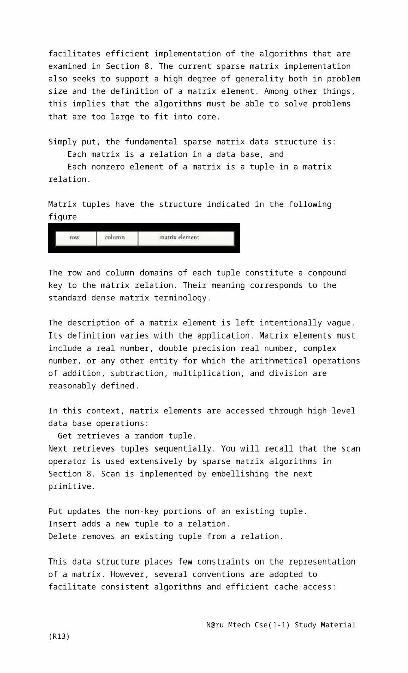
Matrix tuples have the structure indicated in the following figure

The row and column domains of each tuple constitute a compound key to the matrix relation. Their meaning corresponds to the standard dense matrix terminology.

The description of a matrix element is left intentionally vague. Its definition varies with the application. Matrix elements must include a real number, double precision real number, complex number, or any other entity for which the arithmetical operations of addition, subtraction, multiplication, and division are reasonably defined.

In this context, matrix elements are accessed through high level data base operations: Get retrieves a random tuple.Next retrieves tuples sequentially. You will recall that the scan operator is used extensively by sparse matrix algorithms in Section 8. Scan is implemented by embellishing the next primitive.

Put updates the non-key portions of an existing tuple.Insert adds a new tuple to a relation.Delete removes an existing tuple from a relation.

This data structure places few constraints on the representation of a matrix. However, several conventions are adopted to facilitate consistent algorithms and efficient cache access:

Matrices have one-based indexing, i.e. the row and column indices of an n×n matrix range from 1 to n.

Column zero exists for each row of an asymmetric matrix. Column zero serves as a row header and facilitates row operations. It does not enter into the calculations.

A symmetric matrix matrix is stored as an upper triangular matrix. In this representation, the diagonal element anchors row operations as well as entering into the computations. Column zero is not used for symmetric matrices.

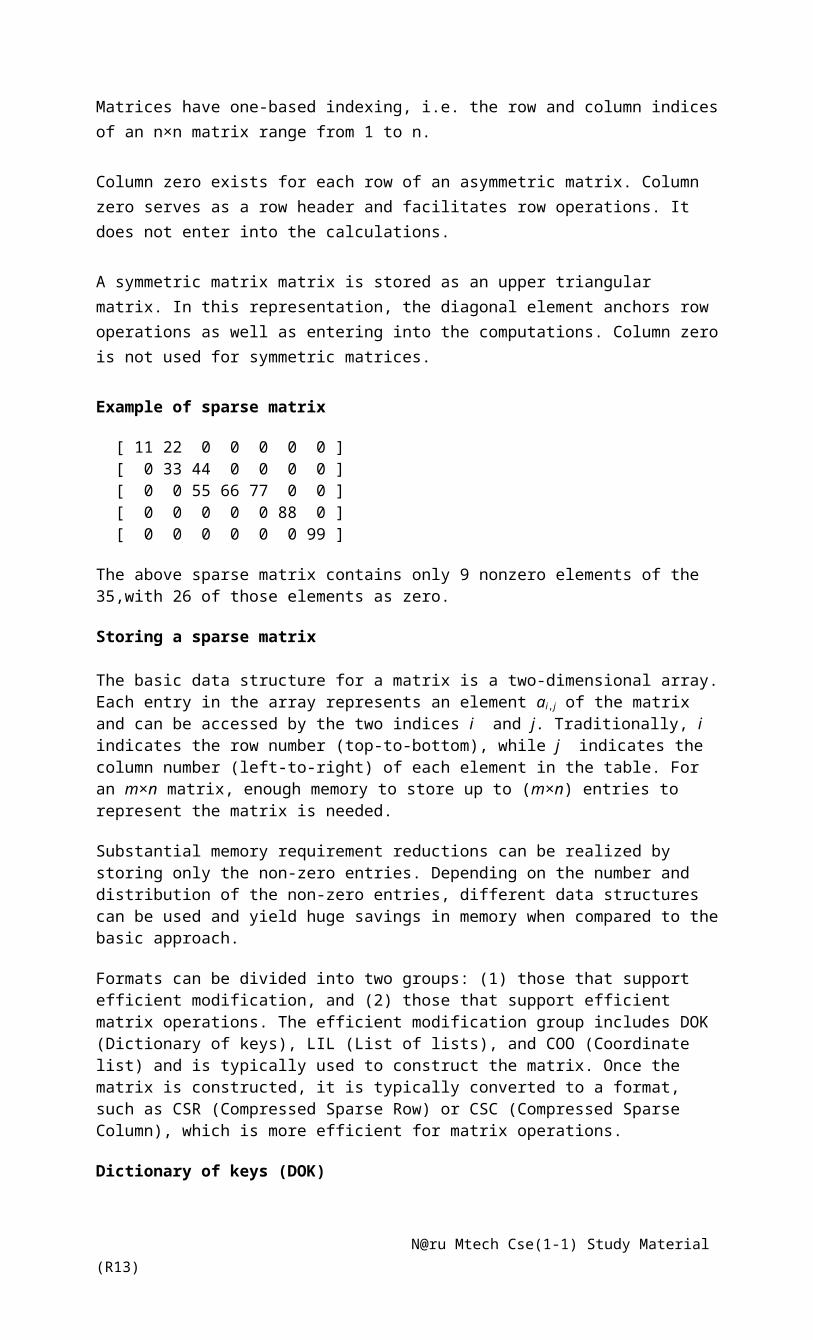
Example of sparse matrix


[ 11 22 0 0 0 0 0 ] [ 0 33 44 0 0 0 0 ] [ 0 0 55 66 77 0 0 ] [ 0 0 0 0 0 88 0 ] [ 0 0 0 0 0 0 99 ]

The above sparse matrix contains only 9 nonzero elements of the 35,with 26 of those elements as zero.

Storing a sparse matrix

The basic data structure for a matrix is a two-dimensional array. Each entry in the array represents an element ai,j of the matrix and can be accessed by the two indices i and j. Traditionally, i indicates the row number (top-to-bottom), while j indicates the column number (left-to-right) of each element in the table. For an m×n matrix, enough memory to store up to (m×n) entries to represent the matrix is needed.

Substantial memory requirement reductions can be realized by storing only the non-zero entries. Depending on the number and distribution of the non-zero entries, different data structures can be used and yield huge savings in memory when compared to the basic approach.

Formats can be divided into two groups: (1) those that support efficient modification, and (2) those that support efficient matrix operations. The efficient modification group includes DOK (Dictionary of keys), LIL (List of lists), and COO (Coordinate list) and is typically used to construct the matrix. Once the matrix is constructed, it is typically converted to a format, such as CSR (Compressed Sparse Row) or CSC (Compressed Sparse Column), which is more efficient for matrix operations.

Dictionary of keys (DOK)

DOK represents non-zero values as a dictionary (e.g., a hash table or binary search tree) mapping (row, column)-pairs to values. This format is good for incrementally constructing a sparse array, but poor for iterating over non-zero values in sorted order. One typically creates the matrix with this format, then converts to another format for processing

List of lists (LIL)

LIL stores one list per row, where each entry stores a column index and value. Typically, these entries are kept sorted by column index for faster lookup. This is another format which is good for incremental matrix construction.

Coordinate list (COO)

COO stores a list of (row, column, value) tuples. Ideally, the entries are sorted (by row index, then column index) to improve random access times. This is another format which is good for incremental matrix construction.

JNTU Previous Questions

1. Explain Big-O-Notation and its properties [Sept 2010]Ans: Refer Unit 1 and Question no.32. Explain about O-mega and Theta Notations. [March 2010]Ans: Refer Unit 1 and Question no.33. How can you do insert, delete operations in Doubly Linked List? [March 2010]Ans: Refer Unit 1 and Question no.74. Explain the characteristics of algorithms. [May 2012]Ans: Refer Unit 1 and Question no.15. How algorithm’s performance is analyzed? Explain. [March 2011]Ans: Refer Unit 1 and Question no.2


http://en.wikipedia.org/wiki/Ordered_pair

http://en.wikipedia.org/wiki/Binary_search_tree

http://en.wikipedia.org/wiki/Hash_table

http://en.wikipedia.org/wiki/Computer_storage

http://en.wikipedia.org/wiki/Array_data_structure

6. Briefly explain the linked representation of a linear list and also discuss operations on it.[May 2012]

Ans: Refer Unit 1 and Question no.4

UNIT – 2

Contents:1. Explain in detail about “Stack ADT”?

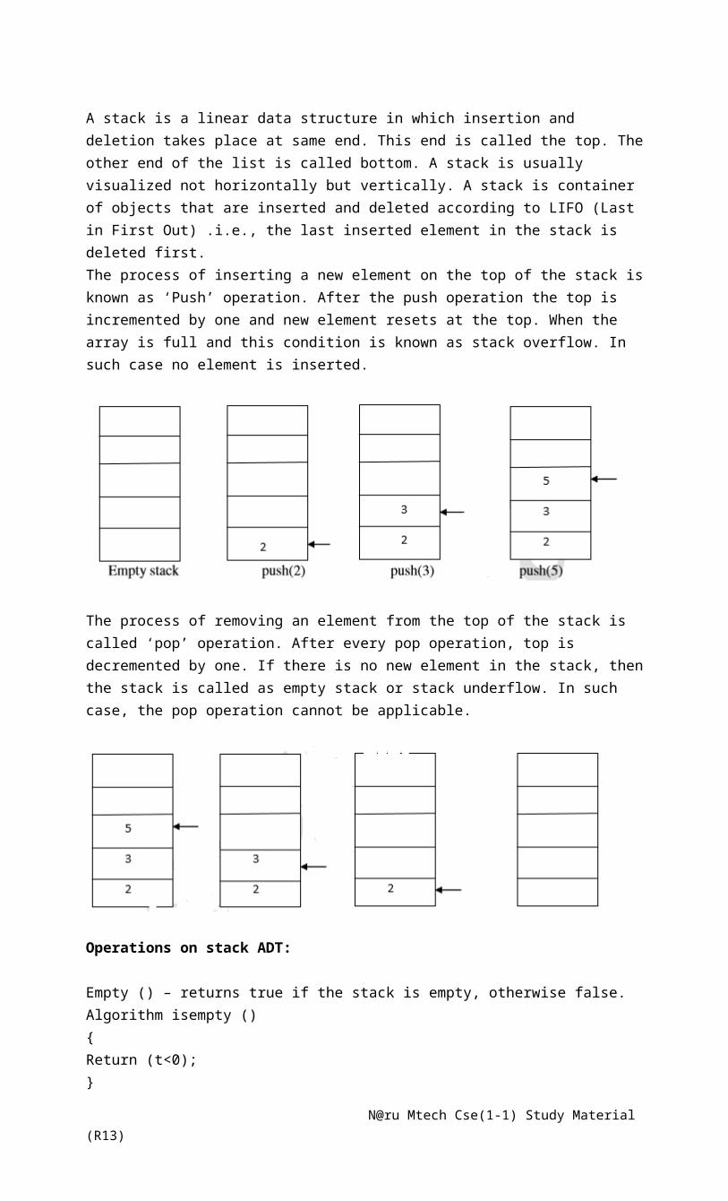
A stack is a linear data structure in which insertion and deletion takes place at same end. This end is called the top. The other end of the list is called bottom. A stack is usually visualized not horizontally but vertically. A stack is container of objects that are inserted and deleted according to LIFO (Last in First Out) .i.e., the last inserted element in the stack is deleted first. The process of inserting a new element on the top of the stack is known as ‘Push’ operation. After the push operation the top is incremented by one and new element resets at the top. When the array is full and this condition is known as stack overflow. In such case no element is inserted.

The process of removing an element from the top of the stack is called ‘pop’ operation. After every pop operation, top is decremented by one. If there is no new element in the stack, then the stack is called as empty stack or stack underflow. In such case, the pop operation cannot be applicable.

Operations on stack ADT:

Empty () – returns true if the stack is empty, otherwise false. Algorithm isempty () { Return (t<0); } Size() - returns the number of elements in the stack Algorithm size() {


Return t+1;}Top() - returns the top element of the stack Algorithm top() { If isempty() then Throw StackEmptyException; Return s[t]; } Pop() - deletes the top element from the stack Algorithm pop() { If isempty() then Throw StackEmptyException; a<- s[t]; t<- t-1; return a; } Push(x) - add the element ‘x’ to top of the stack. Algorithm Push(a) { if size() = N then Throw StackEmptyException; Else t<-t+1; s[t]<-a; } The time complexity of stack to perform all its operations is O(1).

a) Array Implementation of Stack ADT

A Stack Interfacepublic interfaceStack { public void push(Object ob);

public Object pop(); public Object peek(); public boolean isEmpty(); public int size(); }

An ArrayStack Class

public class ArrayStack implements Stack { private Object a[]; private int top; // stack top public ArrayStack(int n) // constructor { a = new Object[n]; // create stack array top = -1; // no items in the stack } public void push(Object item) // add an item on top of stack { if(top == a.length-1) { System.out.println("Stack is full"); return; } top++; // increment top a[top] = item; // insert an item


} public Object pop() // remove an item from top of stack { if( isEmpty() ) { System.out.println("Stack is empty"); return null; } Object item = a[top]; // access top item top--; // decrement top return item; } public Object peek() // get top item of stack { if( isEmpty() ) return null; return a[top]; } public boolean isEmpty() // true if stack is empty { return (top == -1); } public int size() // returns number of items in the stack { return top+1; } }Testing ArrayStack Class

class ArrayStackDemo { public static void main(String[] args) { ArrayStack stk = new ArrayStack(4); // create stack of size 4 Object item; stk.push('A'); // push 3 items onto stack stk.push('B'); stk.push('C'); System.out.println("size(): "+ stk.size()); item = stk.pop(); // delete item System.out.println(item + " is deleted"); stk.push('D'); // add three more items to the stack stk.push('E'); stk.push('F'); System.out.println(stk.pop() + " is deleted"); stk.push('G'); // push one item item = stk.peek(); // get top item from the stack System.out.println(item + " is on top of stack"); } }

b) Linked List Implementation of Stack ADT

public class LinkedStack implements Stack { private class Node { public Object data; public Node next; public Node(Object data, Node next) { this.data = data; this.next = next; } } private Node top = null; public void push(Object item) { top = new Node(item, top); } public Object pop() {


Object item = peek(); top = top.next; return item; } public boolean isEmpty() { return top == null; } public Object peek() { if (top == null) { throw new NoSuchElementException(); } return top.data; } public int size() { int count = 0; for (Node node = top; node != null; node = node.next) { count++; } return count; }}

2. Explain in detail about “Queue ADT”?

A queue is a linear, sequential list of items that are accessed in the order First in First out (FIFO) i.e., the first item inserted in a queue is also one to be deleted. The insertion of element to queue is done at one end called ‘rear’, and deletion or access of element from the queue will be done at other end called ‘front’.

After dequeue, which returns 2


After dequeue, which returns 4

Operations on queue ADT Size() - returns the number of elements in the queue Algorithm size() { Return (f+r); } Empty() - returns whether queue is empty Algorithm empty() { Return (f=r); } Front() - returns the first element in the queue Algorithm front() { if isempty() then Throw QueueEmptyException; return a[f]; } Enqueue() - insert an element to the queue Algorithm enqueue() { if isempty() then Throw QueueEmptyException; temp<- q[f]; f<-f+1; return temp; }Dequeue() – delete the element from the queue Algorithm dequeue() { If size()= N-1 then Throw QueueFullException; Else q[r] <-a; r<- r+1; } The time complexity to perform above operations is O(1)

a) Array Representation of Queue ADT:

import java.io.*; import java.lang.*; class clrqueue


{ DataInputStream get=new DataInputStream(System.in); int a[]; int i,front=0,rear=0,n,item,count=0; void getdata() { try { System.out.println("Enter the limit"); n=Integer.parseInt(get.readLine()); a=new int[n]; } catch(Exception e) { System.out.println(e.getMessage()); } } void enqueue() { try { if(count<n) { System.out.println("Enter the element to be added:"); item=Integer.parseInt(get.readLine()); a[rear]=item; rear++; count++; } else System.out.println("QUEUE IS FULL"); } catch(Exception e) { System.out.println(e.getMessage()); } } void dequeue() { if(count!=0) { System.out.println("The item deleted is:"+a[front]); front++; count--; } else System.out.println("QUEUE IS EMPTY"); if(rear==n) rear=0; } void display() { int m=0; if(count==0)


System.out.println("QUEUE IS EMPTY"); else { for(i=front;m<count;i++,m++) System.out.println(" "+a[i%n]); } } } class myclrqueue { public static void main(String arg[]) { DataInputStream get=new DataInputStream(System.in); int ch; clrqueue obj=new clrqueue(); obj.getdata(); try { do { System.out.println(" 1.Enqueue 2.Dequeue 3.Display 4.Exit"); System.out.println("Enter the choice"); ch=Integer.parseInt(get.readLine()); switch (ch) { case 1: obj.enqueue(); break; case 2: obj.dequeue(); break; case 3: obj.display(); break; } } while(ch!=4); } catch(Exception e) { System.out.println(e.getMessage()); } } }

b) Linked List Representation of QUEUE ADT

import java.io.*;class Node{ public int item; public Node next; public Node(int val) {


item = val; }}class LinkedList{ private Node front,rear; public LinkedList() { front = null; rear = null; } public void insert(int val) { Node newNode = new Node(val); if (front == null) { front = rear = newNode; } else { rear.next = newNode; rear = newNode; } } public int delete() { if(front==null) { System.out.println("Queue is Empty"); return 0; } else { int temp = front.item; front = front.next; return temp; } } public void display() { if(front==null) { System.out.println("Queue is Empty"); } else { System.out.println("Elements in the Queue"); Node current = front; while(current != null) { System.out.println("[" + current.item + "] "); current = current.next; } System.out.println(""); } }


}

class QueueLinkedList{ public static void main(String[] args) throws IOException { LinkedList ll = new LinkedList(); System.out.println("1INSERT\n2.DELETE\n3.DISPLAY"); while(true) { System.out.println("Enter the Key of the Operation"); int c=Integer.parseInt((new BufferedReader(new InputStreamReader(System.in))).readLine()); switch(c) { case 1: System.out.println("Enter the Element"); int val=Integer.parseInt((new BufferedReader(new InputStreamReader(System.in))).readLine()); ll.insert(val); break; case 2: int temp=ll.delete(); if(temp!=0) System.out.println("Element deleted is [" + temp + "] "); break; case 3: ll.display(); break; case 4: System.exit(0); default: System.out.println("You have entered invalid Key.\n Try again"); } } }}3. Explain in detail about “Circular Queue”?

A circular queue is a particular implementation of a queue. It is very efficient. It is also quite useful in low level code, because insertion and deletion are totally independent, which means that you don’t have to worry about an interrupt handler trying to do an insertion at the same time as your main code is doing a deletion.

A circular queue consists of an array that contains the items in the queue, two array indexes and an optional length. The indexes are called the head and tail pointers. Is the queue empty or full?There is a problem with this: Both an empty queue and a full queue would be indicated by having the head and tail point to the same element. There are two ways around this: either maintain a variable with the number of items in the queue, or create the array with one more element that you will actually need so that the queue is never full.Operations


Insertion and deletion are very simple.To insert, write the element to the tail index and increment the tail, wrapping if necessary. To delete, save the head element and increment the head, wrapping if necessary.

A circular buffer first starts empty and of some predefined length. For example, this is a 7-element buffer:

Assume that a 1 is written into the middle of the buffer (exact starting location does not matter in a circular buffer):

Then assume that two more elements are added — 2 & 3 — which get appended after the 1:

If two elements are then removed from the buffer, the oldest values inside the buffer are removed. The two elements removed, in this case, are 1 & 2 leaving the buffer with just a 3:

If the buffer has 7 elements then it is completely full:

A consequence of the circular buffer is that when it is full and a subsequent write is performed, then it starts overwriting the oldest data. In this case, two more elements — A & B — are added and they overwrite the 3 & 4:

Alternatively, the routines that manage the buffer could prevent overwriting the data and return an error or raise an exception. Whether or not data is overwritten is up to the semantics of the buffer routines or the application using the circular buffer.

Finally, if two elements are now removed then what would be returned is not 3 & 4 but 5 & 6 because A & B overwrote the 3 & the 4 yielding the buffer with:

A Java Program for Circular Queue

import java.io.*;

import java.lang.*;

class clrqueue

{

DataInputStream get=new DataInputStream(System.in);

int a[];


int i,front=0,rear=0,n,item,count=0;

void getdata()

{

try

{

System.out.println("Enter the limit");

n=Integer.parseInt(get.readLine());

a=new int[n];

}

catch(Exception e)

{

System.out.println(e.getMessage());

}

}

void enqueue()

{

try

{

if(count<n)

{

System.out.println("Enter the element to be added:");

item=Integer.parseInt(get.readLine());

a[rear]=item;

rear++;

count++;

}

else

System.out.println("QUEUE IS FULL");

}

catch(Exception e)

{


}


}

void dequeue()

{

if(count!=0)

{

System.out.println("The item deleted is:"+a[front]);

front++;

count--;

}

else

System.out.println("QUEUE IS EMPTY");

if(rear==n)

rear=0;

}

void display()

{

int m=0;

if(count==0)

System.out.println("QUEUE IS EMPTY");

else

{

for(i=front;m<count;i++,m++)

System.out.println(" "+a[i%n]);

}

}

}

class myclrqueue

{

public static void main(String arg[])

{

DataInputStream get=new DataInputStream(System.in);

int ch;

clrqueue obj=new clrqueue();


obj.getdata();

try

{

do

{

System.out.println(" 1.Enqueue 2.Dequeue 3.Display 4.Exit");

System.out.println("Enter the choice");

ch=Integer.parseInt(get.readLine());

switch (ch)

{

case 1:

obj.enqueue();

break;

case 2:

obj.dequeue();

break;

case 3:

obj.display();

break;

}

}

while(ch!=4);

}

catch(Exception e)

{


}

}

}

4. Explain in detail about “Dequeue ADT”?

A double-ended queue or dequeue is simply a combination of a stack and a queue in that items can be inserted or removed from both ends.

“double-ended queue” – queue-like linear data structure


http://notes.komputerwiz.net:8000/wiki/Queue_(ADT)

http://notes.komputerwiz.net:8000/wiki/Stack_(ADT)

that supports insertion and deletion of items at both ends of the queue richer ADT than both the queue and the stack ADT

Functions int size() — Returns how many items are in the deque. bool isEmpty() — Returns whether the deque is empty (i.e. size is 0).

void insertFirst(Object o) — Puts an object at the front.

void insertLast(Object o) — Puts an object at the back.

Object removeFirst() — Removes the object from the front and returns it.

Object removeLast() — Removes the object from the back and returns it.

Object first() — Peeks at the front item without removing it.

Object last() — Peeks at the back item without removing it.

Singly Linked List implementation – Inefficient! Removal at the rear takes Θ(n) time.

Doubly Linked List implementation – each node has “prev” and “next” link, hence all operations run at O(1) time

Run Time – Good! all methods run in constant O(1) timeSpace Usage – Good! O(n), n – current no of elements in the stack

A java Program for DEQUEUE ADT.

import java.lang.reflect.Array; class Deque<Item> { private int maxSize=100; private final Item[] array; private int front,rear; private int numberOfItems; public Deque() { array=(Item[])(new Object[maxSize]); front=0; rear=-1; numberOfItems=0; } public boolean isEmpty() { return (numberOfItems==0); } public void addFirst(Item item) { if(front==0) front=maxSize;


array[--front]=item; numberOfItems++; } public void addLast(Item item) { if(rear==maxSize-1) rear=-1; array[++rear]=item; numberOfItems++; } public Item removeFirst() { Item temp=array[front++]; if(front==maxSize) front=0; numberOfItems--; return temp; } public Item removeLast() { Item temp=array[rear--]; if(rear==-1) rear=maxSize-1; numberOfItems--; return temp; } public int getFirst() { return front; } public int getLast() { return rear; } public static void main(String[] args) { Deque<String> element1=new Deque<String>(); Deque<String> element2=new Deque<String>(); for(int i=0;i<args.length;i++) element1.addFirst(args[i]); try { for(;element1.numberOfItems+1>0;) { String temp=element1.removeFirst(); System.out.println(temp); } } catch(Exception ex) { System.out.println("End Of Execution due to remove from empty queue"); } System.out.println(); for(int i=0;i<args.length;i++) element2.addLast(args[i]);


try { for(;element2.numberOfItems+1>0;) { String temp=element2.removeLast(); System.out.println(temp); } } catch(Exception ex) { System.out.println("End Of Execution due to remove from empty queue"); } }

5. Write a java program for Infix To Postfix Conversion Using Stack

class InfixToPostfix { java.util.Stack<Character> stk = new java.util.Stack<Character>(); public String toPostfix(String infix) { infix = "(" + infix + ")"; // enclose infix expr within parentheses String postfix = ""; /* scan the infix char-by-char until end of string is reached */ for( int i=0; i<infix.length(); i++) { char ch, item; ch = infix.charAt(i); if( isOperand(ch) ) // if(ch is an operand), then postfix = postfix + ch; // append ch to postfix stringif( ch == '(' ) // if(ch is a left-bracket), then stk.push(ch); // push onto the stack if( isOperator(ch) ) // if(ch is an operator), then { item = stk.pop(); // pop an item from the stack /* if(item is an operator), then check the precedence of ch and item*/ if( isOperator(item) ) { if( precedence(item) >= precedence(ch) ) { stk.push(item); stk.push(ch); } else { postfix = postfix + item; stk.push(ch); } } else { stk.push(item); stk.push(ch); } } // end of if(isOperator(ch)) if( ch == ')' ) { item = stk.pop(); while( item != '(' ) { postfix = postfix + item; item = stk.pop();


} } } // end of for-loop return postfix; } // end of toPostfix() method public boolean isOperand(char c) { return(c >= 'A' && c <= 'Z'); } public boolean isOperator(char c) { return( c=='+' || c=='-' || c=='*' || c=='/' ); } public int precedence(char c) { int rank = 1; // rank = 1 for '*’ or '/' if( c == '+' || c == '-' ) rank = 2; return rank; } } ///////////////////////// InfixToPostfixDemo.java /////////////// class InfixToPostfixDemo { public static void main(String args[]) {InfixToPostfix obj = new InfixToPostfix(); String infix = "A*(B+C/D)-E"; System.out.println("infix: " + infix ); System.out.println("postfix:"+obj.toPostfix(infix) ); }}

6. Explain in detail about “Priority Queue ADT”?

A priority queue is a collection of zero or more elements. Each element has a priority orvalue. There are two types of priority queues:

Ascending Priority Queue (Min)Descending Priority Queue (Max)

Ascending/Min Priority Queue:It is a collection of elements, which are inserted in any order but the smallest i.e., elementwith minimum priority can be removed.

Descending/Min Priority Queue:It is a collection of elements, which are inserted in any order but the largest element i.e.,element with maximum priority can be removed.

Implementation of Priority Queue:The Priority Queue is implemented by using arrays, linked list and heap data structure. TheHeap data structure. The heap data structure is the best way for implementing the priority queueefficiently.

Operations on Priority queue ADT:Empty() - return true iff the queue is emptySize() - return number of elements in the queueTop() - return element with maximum priorityPop() - remove the element with largest priority from the queue or lowest priorityfrom the queuePush(x) - insert the element ‘x’ into the queue

Applications:


These are used for job scheduling in operating system. In network communication, to manage limited band width for transmission, the priority

queueis used.

These are used to manage discrete events in simulation modelling.

7. Explain in detail about “Heaps”?

Heap is a complete binary tree, whose elements is stored at internal nodes and has the keyssatisfying the heap order property. Heap Data structure is of two types:

Max Heap Min Heap

Max Heap: A max heap is a tree in which the values in each node are greater than or equal tothese in its children.

Min Heap: A min heap is a tree in which the values in each node are less than or equal to these inits children.

Heap Operations

Insertion (Push)To insert an element x into heap, we create a hole in the next available location, sinceotherwise tree will not be complete. If x can be placed in the hole without violating the heap order,then we do so and are done. Otherwise we slide the element that is in the hole’s parent node in the hole.The following fig shows that to insert 14. We create a hole in the next available heap location.Inserting 14 in the hole would violate the heap order property. So 31 is slide down into the hole. This


strategy is continued until the correct location for 14 is found.

This general strategy is known as ‘Precolate up’. The new element is percolated up the heapuntil the correct location is found.

Insertion is easily implemented with as shown below:Template <class T>Push(const T &x){If( isfull()){Throw overflow();Int hole = ++overflow();Int hole = ++currentsize;For( ; hole >1 && x< array[hole/2] ; hole=/2)Array[hole]=array[hole/2];Array[hole]=x;}

Deletion (Pop)If the priority queue is ascending or min priority queue, then only smallest is deleted at eachtime. If the priority queue is descending/ max priority queue then only the largest element is deleted ateach time. The following example shows deleting the smallest element for the previous priority queue.i.e., 13

Initially


The code to implement pop() isTemplate <class T>Pop(){If( isempty())Throw undeflow();T lastelement = heap[ heapsize--];Int currentnode=1;Child=2;While(child< = heapsize){If(child < heapsize && heap[child] < heap [child+1])Child++;If(lastelement > = heap [child])Break;Heap[currentnode] = heap [child];Currentnode = child;


Child = *2}Heap[currentnode]=lastelemnt;}The time complexity to perform above operations is O(logn).

8. Explain in detail about Java.Util Package-Arraylist, Linked List, Vector Classes,stack, queue and iterators.

Java.Util Package-Arraylist

The java.util.ArrayList class provides resizable-array and implements the List interface.Following are the important points about ArrayList:

It implements all optional list operations and it also permits all elements, includes null. It provides methods to manipulate the size of the array that is used internally to store the

list.

The constant factor is low compared to that for the LinkedList implementation.

Class declaration

Following is the declaration for java.util.ArrayList class:

public class ArrayList<E> extends AbstractList<E> implements List<E>, RandomAccess, Cloneable, Serializable

Here <E> represents an Element. For example, if you're building an array list of Integers then you'd initialize it as

ArrayList<Integer> list = new ArrayList<Integer>();

Class constructorsS.N. Constructor & Description1 ArrayList()

This constructor is used to create an empty list with an initial capacity sufficient to hold 10 elements.

2 ArrayList(Collection<? extends E> c)This constructor is used to create a list containing the elements of the specified collection.

3 ArrayList(int initialCapacity)This constructor is used to create an empty list with an initial capacity.

Class methodsS.N. Method & Description1 boolean add(E e)

This method appends the specified element to the end of this list.2 void add(int index, E element)

This method inserts the specified element at the specified position in this list.3 boolean addAll(Collection<? extends E> c)

This method appends all of the elements in the specified collection to the end of this list, in the order that they are returned by the specified collection's Iterator

4 boolean addAll(int index, Collection<? extends E> c)


This method inserts all of the elements in the specified collection into this list, starting at the specified position.

5 void clear()This method removes all of the elements from this list.

6 Object clone()This method returns a shallow copy of this ArrayList instance.

Java.Util Package-Linkedlist

The java.util.LinkedList class operations perform we can expect for a doubly-linked list. Operations that index into the list will traverse the list from the beginning or the end, whichever is closer to the specified index.

Class declaration

Following is the declaration for java.util.LinkedList class:

public class LinkedList<E>

extends AbstractSequentialList<E>

implements List<E>, Deque<E>, Cloneable, Serializable

Parameters

Following is the parameter for java.util.LinkedList class:

E -- This is the type of elements held in this collection.

Field

Fields inherited from class java.util.AbstractList.

Class constructorsS.N. Constructor & Description

1LinkedList() This constructs constructs an empty list.

2LinkedList(Collection<? extends E> c) This constructs a list containing the elements of the specified collection, in the order they are returned by the collection's iterator.

Class methodsS.N. Method & Description

1boolean add(E e)This method appends the specified element to the end of this list.

2void add(int index, E element)This method inserts the specified element at the specified position in this list.

3boolean addAll(Collection<? extends E> c) This method appends all of the elements in the specified collection to the end of this list, in the order that they are returned by the specified collection's iterator.

4boolean addAll(int index, Collection<? extends E> c) This method inserts all of the elements in the specified collection into this list, starting at the specified position.

5void addFirst(E e) This method returns inserts the specified element at the beginning of this list..


http://www.tutorialspoint.com/java/util/linkedlist_addfirst.htm

http://www.tutorialspoint.com/java/util/linkedlist_addall_collection.htm

http://www.tutorialspoint.com/java/util/linkedlist_addall.htm

http://www.tutorialspoint.com/java/util/linkedlist_add_index.htm

http://www.tutorialspoint.com/java/util/linkedlist_add.htm

6void addLast(E e) This method returns appends the specified element to the end of this list.

7void clear() This method removes all of the elements from this list.

8Object clone() This method returns returns a shallow copy of this LinkedList.

9boolean contains(Object o) This method returns true if this list contains the specified element.

10Iterator<E> descendingIterator() This method returns an iterator over the elements in this deque in reverse sequential order.

Java.Util Package-Vector Classes

The java.util.Vector class implements a growable array of objects. Similar to an Array, it contains components that can be accessed using an integer index.

Following are the important points about Vector:

The size of a Vector can grow or shrink as needed to accommodate adding and removing items.

Each vector tries to optimize storage management by maintaining a capacity and a capacityIncrement.

As of the Java 2 platform v1.2, this class was retrofitted to implement the List interface.

Unlike the new collection implementations, Vector is synchronized.

This class is a member of the Java Collections Framework.

Class declaration

Following is the declaration for java.util.Vector class:

public class Vector<E> extends AbstractList<E> implements List<E>, RandomAccess, Cloneable, Serializable

Here <E> represents an Element, which could be any class. For example, if you're building an array list of Integers then you'd initialize it as follows:

ArrayList<Integer> list = new ArrayList<Integer>();

Class constructorsS.N. Constructor & Description1 Vector()

This constructor is used to create an empty vector so that its internal data array has size 10 and its standard capacity increment is zero.

2 Vector(Collection<? extends E> c)This constructor is used to create a vector containing the elements of the specified collection, in the order they are returned by the collection's iterator.

3 Vector(int initialCapacity)This constructor is used to create an empty vector with the specified initial capacity and with its capacity increment equal to zero.

4 Vector(int initialCapacity, int capacityIncrement)


http://www.tutorialspoint.com/java/util/linkedlist_descendingiterator.htm

http://www.tutorialspoint.com/java/util/linkedlist_contains.htm

http://www.tutorialspoint.com/java/util/linkedlist_clone.htm

http://www.tutorialspoint.com/java/util/linkedlist_clear.htm

http://www.tutorialspoint.com/java/util/linkedlist_addlast.htm

This constructor is used to create an empty vector with the specified initial capacity and capacity increment.

Class methods

S.N. Method & Description1 boolean add(E e)

This method appends the specified element to the end of this Vector.2 void add(int index, E element)

This method inserts the specified element at the specified position in this Vector.3 boolean addAll(Collection<? extends E> c)

This method appends all of the elements in the specified Collection to the end of this Vector.4 boolean addAll(int index, Collection<? extends E> c)

This method inserts all of the elements in the specified Collection into this Vector at the specified position.

5 void addElement(E obj)This method adds the specified component to the end of this vector, increasing its size by

one.6 int capacity()

This method returns the current capacity of this vector.7 void clear()

This method removes all of the elements from this vector.8 clone clone()

This method returns a clone of this vector.9 boolean contains(Object o)

This method returns true if this vector contains the specified element.

Java.Util Package-Stacks

The java.util.Stack class represents a last-in-first-out (LIFO) stack of objects.

When a stack is first created, it contains no items.

In this class, the last element inserted is accessed first.

Class declaration

Following is the declaration for java.util.Stack class:

public class Stack<E> extends Vector<E>

Class constructors

S.N. Constructor & Description1 Stack()

This constructor creates an empty stack.

Class methods

S.N. Method & Description1 boolean empty()

This method tests if this stack is empty.2 E peek()

This method looks at the object at the top of this stack without removing it from the stack.3 E pop()

This method removes the object at the top of this stack and returns that object as the value of this function.4 E push(E item)

This method pushes an item onto the top of this stack.5 int search(Object o)

This method returns the 1-based position where an object is on this stack.

____________________________________________________________________________________


Java.util.Interfaces

The java.util.Interfaces contains the collections framework, legacy collection classes, event model, date and time facilities, internationalization, and miscellaneous utility classes (a string tokenizer, a random-number generator, and a bit array).

S.N. Intreface & Description

1 Deque<E> This is a linear collection that supports element insertion and removal at both ends.2 Enumeration<E> This is an object that implements the Enumeration interface generates a series of elements, one at a time.3 EventListener This is a tagging interface that all event listener interfaces must extend.4 Formattable This is the Formattable interface must be implemented by any class that needs to perform custom formatting using the 's' conversion specifier of Formatter. 5 Iterator<E> This is an iterator over a collection.6 Queue<E> This is a collection designed for holding elements prior to processing.

JNTU PREVIOUS QUESTIONS1. Implement a Queue as a Linked List. [MARCH 2010]Ans: Refer Unit 2 Question No.22. Write short notes on Priority Queues. [SEPT 2010] [APR 2011][APR 2012]Ans: Refer Unit 2 Question No.63. Discuss in detail about the stacks. [NOV 2011]Ans: Refer Unit 2 Question No.1


UNIT – 3

CONTENTS

1) Explain in detail about “LINEAR SEARCH”?

Linear search or sequential search is a method for finding a particular value in a list that consists of checking every one of its elements, one at a time and in sequence, until the desired one is found.

Linear search is the simplest search algorithm; it is a special case of brute-force search. Its worst case cost is proportional to the number of elements in the list; and so is its expected cost, if all list elements are equally likely to be searched for.

Analysis

For a list with n items, the best case is when the value is equal to the first element of the list, in which case only one comparison is needed. The worst case is when the value is not in the list (or occurs only once at the end of the list), in which case n comparisons are needed.

If the value being sought occurs k times in the list, and all orderings of the list are equally likely, the expected number of comparisons is

For example, if the value being sought occurs once in the list, and all orderings of the list are

equally likely, the expected number of comparisons is However, if it is known that it occurs once, then at most n - 1 comparisons are needed, and the expected number of comparisons

is

Application

Linear search is usually very simple to implement, and is practical when the list has only a few elements, or when performing a single search in an unordered list.


http://en.wikipedia.org/wiki/Average-case_complexity

http://en.wikipedia.org/wiki/Worst-case_complexity

http://en.wikipedia.org/wiki/Worst-case_complexity

http://en.wikipedia.org/wiki/Brute-force_search

http://en.wikipedia.org/wiki/Search_algorithm

http://en.wikipedia.org/wiki/List_(computing)

When many values have to be searched in the same list, it often pays to pre-process the list in order to use a faster method. For example, one may sort the list and use binary search, or build any efficient search data structure from it. Should the content of the list change frequently, repeated re-organization may be more trouble than it is worth.

As a result, even though in theory other search algorithms may be faster than linear search (for instance binary search), in practice even on medium sized arrays (around 100 items or less) it might be infeasible to use anything else. On larger arrays, it only makes sense to use other, faster search methods if the data is large enough, because the initial time to prepare (sort) the data is comparable to many linear searches

Program in Java

import java.util.Scanner; class LinearSearch { public static void main(String args[]) { int c, n, search, array[]; Scanner in = new Scanner(System.in); System.out.println("Enter number of elements"); n = in.nextInt(); array = new int[n]; System.out.println("Enter " + n + " integers"); for (c = 0; c < n; c++) array[c] = in.nextInt(); System.out.println("Enter value to find"); search = in.nextInt(); for (c = 0; c < n; c++) { if (array[c] == search) /* Searching element is present */ { System.out.println(search + " is present at location " + (c + 1) + "."); break; } } if (c == n) /* Searching element is absent */ System.out.println(search + " is not present in array."); }}

2) Explain in detail about “BINARY SEARCH”?

A Binary search or half-interval search algorithm finds the position of a specified input value (the search "key") within an array sorted by key value. In each step, the algorithm compares the search key value with the key value of the middle element of the array. If the keys match, then a matching element has been found and its index, or position, is returned. Otherwise, if the search key is less than the middle element's key, then the algorithm repeats its action on the sub-array to the left of the middle element or, if the search key is greater, on the sub-array to the right. If the


http://en.wikipedia.org/wiki/Sorted_array

http://en.wikipedia.org/wiki/Algorithm

http://en.wikipedia.org/wiki/Binary_search

http://en.wikipedia.org/wiki/Search_data_structure

http://en.wikipedia.org/wiki/Sort_(computing)

remaining array to be searched is empty, then the key cannot be found in the array and a special "not found" indication is returned.

A binary search halves the number of items to check with each iteration, so locating an item (or determining its absence) takes logarithmic time. A binary search is a dichotomic divide and conquer search algorithm.

Performance

With each test that fails to find a match at the probed position, the search is continued with one or other of the two sub-intervals, each at most half the size. More precisely, if the number of items, N, is odd then both sub-intervals will contain (N−1)/2 elements, while if N is even then the two sub-intervals contain N/2−1 and N/2 elements.

If the original number of items is N then after the first iteration there will be at most N/2 items remaining, then at most N/4 items, at most N/8 items, and so on. In the worst case, when the value is not in the list, the algorithm must continue iterating until the span has been made empty;

this will have taken at most ⌊log2(N)+1⌋ iterations, where the ⌊ ⌋ notation denotes the floor function that rounds its argument down to an integer. This worst case analysis is tight: for any N

there exists a query that takes exactly ⌊log2(N)+1⌋ iterations. When compared to linear search, whose worst-case behaviour is N iterations, we see that binary search is substantially faster as N grows large. For example, to search a list of one million items takes as many as one million iterations with linear search, but never more than twenty iterations with binary search. However, a binary search can only be performed if the list is in sorted order.

Program in Java

import java.util.Scanner; class BinarySearch { public static void main(String args[]) { int c, first, last, middle, n, search, array[]; Scanner in = new Scanner(System.in); System.out.println("Enter number of elements"); n = in.nextInt(); array = new int[n]; System.out.println("Enter " + n + " integers"); for (c = 0; c < n; c++) array[c] = in.nextInt(); System.out.println("Enter value to find"); search = in.nextInt(); first = 0; last = n - 1; middle = (first + last)/2; while( first <= last ) { if ( array[middle] < search ) first = middle + 1;


http://en.wikipedia.org/wiki/Linear_search

http://en.wikipedia.org/wiki/Binary_logarithm

http://en.wikipedia.org/wiki/Worst_case_analysis

http://en.wikipedia.org/wiki/Floor_function

http://en.wikipedia.org/wiki/Floor_function

http://en.wikipedia.org/wiki/Binary_logarithm

http://en.wikipedia.org/wiki/Search_algorithm

http://en.wikipedia.org/wiki/Divide_and_conquer_algorithm


http://en.wikipedia.org/wiki/Dichotomic_search

http://en.wikipedia.org/wiki/Logarithmic_time

else if ( array[middle] == search ) { System.out.println(search + " found at location " + (middle + 1) + "."); break; } else last = middle - 1; middle = (first + last)/2; } if ( first > last ) System.out.println(search + " is not present in the list.\n"); }}

3) Explain In detail about ‘HASHING Techniques’?

A hash function is any algorithm that maps data of a variable length to data of a fixed length. The values returned by a hash function are called hash values, hash codes, hash sums, checksums or simply hashes.

Hash functions are primarily used to generate fixed-length output data that acts as a shortened reference to the original data. This is useful when the original data is too cumbersome to use in its entirety.

One practical use is a data structure called a hash table where the data is stored associatively. Searching linearly for a person's name in a list becomes cumbersome as the length of the list increases, but the hashed value can be used to store a reference to the original data and retrieve constant time (barring collisions). Another use is in cryptography, the science of encoding and safeguarding data. It is easy to generate hash values from input data and easy to verify that the data matches the hash, but hard to 'fake' a hash value to hide malicious data. This is the principle behind the Pretty Good Privacy algorithm for data validation.

Hash functions are also frequently used to accelerate table lookup or data comparison tasks such as finding items in a database, detecting duplicated or similar records in a large file and finding similar stretches in DNA sequences.

A hash function should be deterministic: when it is invoked twice on pieces of data that should be considered equal (e.g., two strings containing exactly the same characters), the function should produce the same value. This is crucial to the correctness of virtually all algorithms based on hashing. In the case of a hash table, the lookup operation should look at the slot where the insertion algorithm actually stored the data that is being sought for, so it needs the same hash value.

Hash functions are typically not invertible, meaning that it is not possible to reconstruct the input datum x from its hash value h(x) alone. In many applications, it is common that several values hash to the same value, a condition called a hash collision. Since collisions cause "confusion" of objects, which can make exact hash-based algorithm slower approximate ones less precise, hash functions are designed to minimize the probability of collisions. For cryptographic uses, hash functions are engineered in such a way that is impossible to reconstruct any input from the hash alone without expending great amounts of computing time (see also One-way function).

Hash functions are related to (and often confused with) checksums, check digits, fingerprints, randomization functions, error-correcting codes, and cryptographic. Although these concepts overlap to some extent, each has its own uses and requirements and is designed and optimized


http://en.wikipedia.org/wiki/One-way_function

http://en.wikipedia.org/wiki/Inverse_function

http://en.wikipedia.org/wiki/Deterministic_algorithm

http://en.wikipedia.org/wiki/Pretty_Good_Privacy

http://en.wikipedia.org/wiki/Cryptography


http://en.wikipedia.org/wiki/Checksums

http://en.wikipedia.org/wiki/Data_(computing)

http://en.wikipedia.org/wiki/Algorithm

differently. The Hash Keeper database maintained by the American National Drug Intelligence Center, for instance, is more aptly described as a catalog of file fingerprints than of hash values.

Hash tables

Hash functions are primarily used in hash tables, to quickly locate a data record (e.g., a dictionary definition) given its search key (the headword). Specifically, the hash function is used to map the search key to an index; the index gives the place in the hash table where the corresponding record should be stored. Hash tables, in turn, are used to implement associative arrays and dynamic sets.

Typically, the domain of a hash function (the set of possible keys) is larger than its range (the number of different table indexes), and so it will map several different keys to the same index. Therefore, each slot of a hash table is associated with (implicitly or explicitly) a set of records, rather than a single record. For this reason, each slot of a hash table is often called a bucket, and hash values are also called bucket indices.

Thus, the hash function only hints at the record's location—it tells where one should start looking for it. Still, in a half-full table, a good hash function will typically narrow the search down to only one or two entries.

Hash Table Operations

– Search: compute f(k) and see if a pair exists– Insert: compute f(k) and place it in that position

– Delete: compute f(k) and delete the pair in that position

Ideal Hashing Example

Pairs are: (22,a),(33,c),(3,d),(72,e),(85,f)

Hash table is ht[0:7], b = 8 (where b is the number of positions in the hash table)

Hash function f is key % b = key % 8

Where does (25,g) go? The home bucket for (25,g) is already occupied by (33,c)

à This situation is called collision


http://en.wikipedia.org/wiki/Set_(mathematics)

http://en.wikipedia.org/wiki/Set_(abstract_data_type)



http://en.wikipedia.org/wiki/Primary_key

http://en.wikipedia.org/wiki/Dictionary


Keys that have the same home bucket are called synonyms– 25 and 33 are synonyms with respect to the hash function that is in use

A collision occurs when the home bucket for a new pair is occupied by a pair with different key

An overflow occurs when there is no space in the home bucket for the new pair

When a bucket can hold only one pair, collisions and overflows occur together

Need a method to handle overflows

Hash Table Issues

The choice of hash function Overflow handling

The size (number of buckets) of hash table

Hash Functions

Two parts

1. Convert key into an integer in case the key is not

2. Map an integer into a home bucket

– f(k) is an integer in the range [0,b-1],where b is the number of buckets in the table

Mapping Into a Home Bucket

Most common method is by division

homeBucket = k % divisor

Divisor equals to the number of buckets b 0 <= homeBucket < divisor = b

Overflow Handling

Search the hash table in some systematic fashion for a bucket that is not full

– Linear probing (linear open addressing)– Quadratic probing

– Double Hashing

Eliminate overflows by permitting each bucket to keep a list of all pairs for which it is home bucket

- Hashing with Chains


Linear probing:

In general, our collision resolution strategy is to generate a sequence of hash table slots (probe sequence) that can hold the record; test each slot until find empty one (probing)

For example, D=8, keys a,b,c,d have hash values h(a)=3, h(b)=0, h(c)=4, h(d)=3

Where do we insert d? 3 already filled

Probe sequence using linear hashing:

h1(d) = (h(d)+1)%8 = 4%8 = 4

h2(d) = (h(d)+2)%8 = 5%8 = 5*

h3(d) = (h(d)+3)%8 = 6%8 = 6

etc.

7, 0, 1, 2

Wraps around the beginning of the table!

Linear probing: hi(x) = (h(x) + i) % D

all buckets in table will be candidates for inserting a new record before the probe sequence returns to home position

clustering of records, leads to long probing sequences

Linear probing with skipping: hi(x) = (h(x) + ic) % D

c constant other than 1

records with adjacent home buckets will not follow same probe sequence

Quadratic probing

Quadratic probing is an open addressing scheme in computer programming for resolving collisions in hash tables—when an incoming data's hash value indicates it should be stored in an already-occupied slot or bucket. Quadratic probing operates by taking the original hash index and adding successive values of an arbitrary quadratic polynomial until an open slot is found.

For a given hash value, the indices generated by linear probing are as follows:


http://en.wikipedia.org/wiki/Linear_probing

http://en.wikipedia.org/wiki/Quadratic_polynomial


http://en.wikipedia.org/wiki/Computer_programming

This method results in primary clustering, and as the cluster grows larger, the search for those items hashing within the cluster becomes less efficient.

An example sequence using quadratic probing is:

Quadratic probing can be a more efficient algorithm in a closed hash table, since it better avoids the clustering problem that can occur with linear probing, although it is not immune. It also provides good memory caching because it preserves some locality of reference; however, linear probing has greater locality and, thus, better cache performance.

Quadratic probing is used in the Berkeley Fast File System to allocate free blocks. The allocation routine chooses a new cylinder-group when the current is nearly full using quadratic probing, because of the speed it shows in finding unused cylinder-groups.

Let h(k) be a hash function that maps an element k to an integer in [0,m-1], where m is the size of the table. Let the ith probe position for a value k be given by the function

where c2 ≠ 0. If c2 = 0, then h(k,i) degrades to a linear probe. For a given hash table, the values of c1 and c2 remain constant.

Examples:

If , then the probe sequence will be

For m = 2n, a good choice for the constants are c1 = c2 = 1/2, as the values of h(k,i) for i in [0,m-1] are all distinct. This leads to a probe sequence of

where the values increase by 1, 2, 3, ...

For prime m > 2, most choices of c1 and c2 will make h(k,i) distinct for i in [0, (m-1)/2]. Such choices include c1 = c2 = 1/2, c1 = c2 = 1, and c1 = 0, c2 = 1. Because there are only about m/2 distinct probes for a given element, it is difficult to guarantee that insertions will succeed when the load factor is > 1/2.

Double Hashing

(1) Use one hash function to determine the first slot

(2) Use a second hash function to determine the increment for the probe sequence

h(k,i) = (h1(k) + i h2(k) ) mod m, i=0,1,...

• Initial probe: h1(k)

• Second probe is offset by h2(k) mod m, so on ...

• Advantage: avoids clustering

• Disadvantage: harder to delete an element

• Can generate m2 probe sequences maximum

Hashing with Chains



http://en.wikipedia.org/wiki/Linear_probing

http://en.wikipedia.org/wiki/Hash_function

http://en.wikipedia.org/wiki/Berkeley_Fast_File_System

http://en.wikipedia.org/wiki/Locality_of_reference

http://en.wikipedia.org/wiki/Primary_clustering

Hash table can handle overflows using chaining. Each bucket keeps a chain of all pairs for which it is the home bucket

Program for Hashing In Java.Util Hashtable

HashTest.java public class HashTest {

static BufferedReader reader (String fileName) throws Exception {// Code omitted to save paper.

}

// Arguments are the file of words and the table size.public static void main (String [ ] args) throws Exception {

if (args.length != 2) {System.err.println ("Wrong number of arguments.");System.exit (1);

}BufferedReader wordReader;int tableSize = Integer.parseInt (args[1]);Hashtable table = new Hashtable (tableSize);String word;

// Load the words into the table.int wordCount = 0;wordReader = reader (args[0]);do {

try {word = wordReader.readLine ();

} catch (Exception e) ...if (word == null) {

break;} else {

wordCount++;table.put (word, new Integer(wordCount));

}} while (true);

// Now see how long it takes to look up all the words.wordReader = reader (args[0]);long startTime = System.currentTimeMillis ( );do {

try {word = wordReader.readLine ();

} catch (Exception e) ...if (word == null) {


break;} else {

boolean result = table.containsKey (word);}

} while (true);long finishTime = System.currentTimeMillis ( );System.out.println ("Time to hash " + wordCount + " words is "

+ (finishTime-startTime) + " milliseconds.");table.printStatistics ( );

}}

Hashtable.java public class Hashtable {

private static boolean DEBUGGING = false;private LinkedList [] myTable;

public Hashtable (int size) {myTable = new LinkedList [size];for (int k=0; k<size; k++) {

myTable[k] = new LinkedList ( );}

}

private static long hash (String key) {// Uncomment one of the following lines to use the corresponding hash function.// return hash1 (key);// return hash2 (key);// return hash3 (key);// return Math.abs (key.hashCode ( ));

}

// Slight variation on the ETH hashing algorithmprivate static int MAGIC1 = 257;private static long hash1 (String key) {

long h = 1;for (int k=0; k<key.length(); k++) {

h = ((h % MAGIC1)+1) * (int) key.charAt(k);}return h;

}

// Slight variation on the GNU-cpp hashing algorithmprivate static int MAGIC2 = 4;private static long hash2 (String key) {

long h = 0;for (int k=0; k<key.length(); k++) {

h = MAGIC2 * h + (int) key.charAt(k);}return h << 1 >>> 1;

}

// Slight variation on the GNU-cc1 hashing algorithmprivate static int MAGIC3 = 613;private static long hash3 (String key) {

long h = key.length();for (int k=0; k<key.length(); k++) {

h = MAGIC3 * h + (int) key.charAt(k);}return h << 2 >>> 2;

}


// Add the key to the table. The value is included just for compatibility with// the Hashtable class in java.util.public void put (String key, Integer value) {

int h = (int) (hash (key) % myTable.length);if (!myTable[h].find (key)) {

myTable[h].insert (new Info (key, value));if (DEBUGGING) {

System.out.println ("Inserting " + key);}

} else {System.err.println (key + " already in table.");

}}

// Return true if key is in the table, and false otherwise.public boolean containsKey (String key) {

int h = (int) (hash (key) % myTable.length);return (myTable[h].find(key));

}

// Print statistics about the table:// the maximum length of a collision list;// the optimal length of a collision list;// the average number of comparisons needed for a successful search;// the standard deviation for the number of comparisons needed for// a successful search.public void printStatistics ( ) {

// Code omitted to save paper.}

}// Auxiliary classes follow in the file; code is omitted to save paper.

TTThashTest.java import java.util.*;

public class TTThashTest {// Measure the time to put all possible Tic-tac-toe boards into the hash table.

public static void main (String [ ] args) {Hashtable table = new Hashtable ( );long startTime = System.currentTimeMillis ( );for (int k=0; k<19683; k++) {

TTTboard b = new TTTboard (k);table.put (b, new Integer (k));

}long finishTime = System.currentTimeMillis ( );System.out.println ("Time to insert all Tic-tac-toe boards = "

+ (finishTime-startTime));}

}

Java.Util – Hashmap

java.util

Class HashMap<K,V>

java.lang.Object

java.util.AbstractMap<K,V>


http://docs.oracle.com/javase/7/docs/api/java/util/AbstractMap.html

http://docs.oracle.com/javase/7/docs/api/java/lang/Object.html

java.util.HashMap<K,V>

Type Parameters:

K - the type of keys maintained by this map

V - the type of mapped values

All Implemented Interfaces:

Serializable, Cloneable, Map<K,V>

Direct Known Subclasses:

LinkedHashMap, PrinterStateReasons

public class HashMap<K,V>extends AbstractMap<K,V>implements Map<K,V>, Cloneable, SerializableHash table based implementation of the Map interface. This implementation provides all of the optional map operations, and permits null values and the null key. (The HashMap class is roughly equivalent to Hashtable, except that it is unsynchronized and permits nulls.) This class makes no guarantees as to the order of the map; in particular, it does not guarantee that the order will remain constant over time.

This implementation provides constant-time performance for the basic operations (get and put), assuming the hash function disperses the elements properly among the buckets. Iteration over collection views requires time proportional to the "capacity" of the HashMap instance (the number of buckets) plus its size (the number of key-value mappings). Thus, it's very important not to set the initial capacity too high (or the load factor too low) if iteration performance is important.

An instance of HashMap has two parameters that affect its performance: initial capacity and load factor. The capacity is the number of buckets in the hash table, and the initial capacity is simply the capacity at the time the hash table is created. The load factor is a measure of how full the hash table is allowed to get before its capacity is automatically increased. When the number of entries in the hash table exceeds the product of the load factor and the current capacity, the hash table is rehashed (that is, internal data structures are rebuilt) so that the hash table has approximately twice the number of buckets.

As a general rule, the default load factor (.75) offers a good tradeoff between time and space costs. Higher values decrease the space overhead but increase the lookup cost (reflected in most of the operations of the HashMap class, including get and put). The expected number of entries in the map and its load factor should be taken into account when setting its initial capacity, so as to minimize the number of rehash operations. If the initial capacity is greater than the maximum number of entries divided by the load factor, no rehash operations will ever occur.

If many mappings are to be stored in a HashMap instance, creating it with a sufficiently large capacity will allow the mappings to be stored more efficiently than letting it perform automatic rehashing as needed to grow the table.

Note that this implementation is not synchronized. If multiple threads access a hash map concurrently, and at least one of the threads modifies the map structurally, it must be synchronized externally. (A structural modification is any operation that adds or deletes one or more mappings; merely changing the value associated with a key that an instance already contains is not a structural modification.) This is typically accomplished by synchronizing on some object that naturally encapsulates the map. If no such object exists, the map should be "wrapped" using the Collections.synchronizedMap method. This is best done at creation time, to prevent accidental unsynchronized access to the map:

Map m = Collections.synchronizedMap(new HashMap(...));


http://docs.oracle.com/javase/7/docs/api/java/util/Collections.html#synchronizedMap(java.util.Map)

http://docs.oracle.com/javase/7/docs/api/java/io/Serializable.html

http://docs.oracle.com/javase/7/docs/api/java/lang/Cloneable.html

http://docs.oracle.com/javase/7/docs/api/java/util/Map.html

http://docs.oracle.com/javase/7/docs/api/java/util/AbstractMap.html

http://docs.oracle.com/javase/7/docs/api/javax/print/attribute/standard/PrinterStateReasons.html

http://docs.oracle.com/javase/7/docs/api/java/util/LinkedHashMap.html

http://docs.oracle.com/javase/7/docs/api/java/util/Map.html



The iterators returned by all of this class's "collection view methods" are fail-fast: if the map is structurally modified at any time after the iterator is created, in any way except through the iterator's own remove method, the iterator will throw aConcurrentModificationException. Thus, in the face of concurrent modification, the iterator fails quickly and cleanly, rather than risking arbitrary, non-deterministic behavior at an undetermined time in the future.

Note that the fail-fast behavior of an iterator cannot be guaranteed as it is, generally speaking, impossible to make any hard guarantees in the presence of unsynchronized concurrent modification. Fail-fast iterators throwConcurrentModificationException on a best-effort basis. Therefore, it would be wrong to write a program that depended on this exception for its correctness: the fail-fast behavior of iterators should be used only to detect bugs.

JAVA.Util Hash Set

java.util

Class HashSet<E>

java.lang.Object

java.util.AbstractCollection<E>

java.util.AbstractSet<E>

java.util.HashSet<E>

Type Parameters:

E - the type of elements maintained by this set

All Implemented Interfaces:

Serializable, Cloneable, Iterable<E>, Collection<E>, Set<E>

Direct Known Subclasses:

JobStateReasons, LinkedHashSet

public class HashSet<E>extends AbstractSet<E>implements Set<E>, Cloneable, SerializableThis class implements the Set interface, backed by a hash table (actually a HashMap instance). It makes no guarantees as to the iteration order of the set; in particular, it does not guarantee that the order will remain constant over time. This class permits the null element.

This class offers constant time performance for the basic operations (add, remove, contains and size), assuming the hash function disperses the elements properly among the buckets. Iterating over this set requires time proportional to the sum of the HashSet instance's size (the number of elements) plus the "capacity" of the backing HashMap instance (the number of buckets). Thus, it's very important not to set the initial capacity too high (or the load factor too low) if iteration performance is important.

Note that this implementation is not synchronized. If multiple threads access a hash set concurrently, and at least one of the threads modifies the set, it must be synchronized externally. This is typically accomplished by synchronizing on some object that naturally encapsulates the set. If no such object exists, the set should be "wrapped" using the Collections.synchronizedSet method. This is best done at creation time, to prevent accidental unsynchronized access to the set:

Set s = Collections.synchronizedSet(new HashSet(...));

The iterators returned by this class's iterator method are fail-fast: if the set is modified at any time after the iterator is created, in any way except through the iterator's own remove method, the


http://docs.oracle.com/javase/7/docs/api/java/util/Collections.html#synchronizedSet(java.util.Set)



http://docs.oracle.com/javase/7/docs/api/java/util/Set.html

http://docs.oracle.com/javase/7/docs/api/java/util/AbstractSet.html

http://docs.oracle.com/javase/7/docs/api/java/util/LinkedHashSet.html

http://docs.oracle.com/javase/7/docs/api/javax/print/attribute/standard/JobStateReasons.html

http://docs.oracle.com/javase/7/docs/api/java/util/Set.html

http://docs.oracle.com/javase/7/docs/api/java/util/Collection.html

http://docs.oracle.com/javase/7/docs/api/java/lang/Iterable.html



http://docs.oracle.com/javase/7/docs/api/java/util/AbstractSet.html

http://docs.oracle.com/javase/7/docs/api/java/util/AbstractCollection.html

http://docs.oracle.com/javase/7/docs/api/java/lang/Object.html

http://docs.oracle.com/javase/7/docs/api/java/util/ConcurrentModificationException.html

Iterator throws aConcurrentModificationException. Thus, in the face of concurrent modification, the iterator fails quickly and cleanly, rather than risking arbitrary, non-deterministic behavior at an undetermined time in the future.

Note that the fail-fast behavior of an iterator cannot be guaranteed as it is, generally speaking, impossible to make any hard guarantees in the presence of unsynchronized concurrent modification. Fail-fast iterators throwConcurrentModificationException on a best-effort basis. Therefore, it would be wrong to write a program that depended on this exception for its correctness: the fail-fast behavior of iterators should be used only to detect bugs.

4) Describe Bubble Sorting Technique?

Bubble Sort

Bubble sort, sometimes incorrectly referred to as sinking sort, is a simple sorting algorithm that works by repeatedly stepping through the list to be sorted, comparing each pair of adjacent items and swapping them if they are in the wrong order. The pass through the list is repeated until no swaps are needed, which indicates that the list is sorted. The algorithm gets its name from the way smaller elements "bubble" to the top of the list. Because it only uses comparisons to operate on elements, it is a comparison sort. Although the algorithm is simple, most of the other sorting algorithms are more efficient for large lists.

Bubble sort has worst-case and average complexity both О(n2), where n is the number of items being sorted. There exist many sorting algorithms with substantially better worst-case or average complexity of O(n log n). Even other О(n2) sorting algorithms, such as insertion sort, tend to have better performance than bubble sort. Therefore, bubble sort is not a practical sorting algorithm when n is large.

The only significant advantage that bubble sort has over most other implementations, even quicksort, but not insertion sort, is that the ability to detect that the list is sorted is efficiently built into the algorithm. Performance of bubble sort over an already-sorted list (best-case) is O(n). By contrast, most other algorithms, even those with better average-case complexity, perform their entire sorting process on the set and thus are more complex. However, not only does insertion sort have this mechanism too, but it also performs better on a list that is substantially sorted (having a small number of inversions).

Bubble sort should be avoided in case of large collections. It will not be efficient in case of reverse ordered collection.

Step-by-step example

Let us take the array of numbers "5 1 4 2 8", and sort the array from lowest number to greatest number using bubble sort. In each step, elements written in bold are being compared. Three passes will be required.

First Pass:( 5 1 4 2 8 ) ( 1 5 4 2 8 ), Here, algorithm compares the first two elements, and swaps since 5 > 1.( 1 5 4 2 8 ) ( 1 4 5 2 8 ), Swap since 5 > 4( 1 4 5 2 8 ) ( 1 4 2 5 8 ), Swap since 5 > 2( 1 4 2 5 8 ) ( 1 4 2 5 8 ), Now, since these elements are already in order (8 > 5), algorithm does not swap them.Second Pass:( 1 4 2 5 8 ) ( 1 4 2 5 8 )( 1 4 2 5 8 ) ( 1 2 4 5 8 ), Swap since 4 > 2( 1 2 4 5 8 ) ( 1 2 4 5 8 )( 1 2 4 5 8 ) ( 1 2 4 5 8 )Now, the array is already sorted, but our algorithm does not know if it is completed. The algorithm needs one whole pass without any swap to know it is sorted.


http://en.wikipedia.org/wiki/Inversion_(discrete_mathematics)

http://en.wikipedia.org/wiki/Insertion_sort

http://en.wikipedia.org/wiki/Average-case_complexity


http://en.wikipedia.org/wiki/Quicksort


http://en.wikipedia.org/wiki/Big_o_notation

http://en.wikipedia.org/wiki/Comparison_sort

http://en.wikipedia.org/wiki/Swap_(computer_science)

http://en.wikipedia.org/wiki/Sorting_algorithm

http://docs.oracle.com/javase/7/docs/api/java/util/ConcurrentModificationException.html

Third Pass:( 1 2 4 5 8 ) ( 1 2 4 5 8 )( 1 2 4 5 8 ) ( 1 2 4 5 8 )( 1 2 4 5 8 ) ( 1 2 4 5 8 )( 1 2 4 5 8 ) ( 1 2 4 5 8 )

Java Program for Bubble Sort

import java.util.Scanner; class BubbleSort { public static void main(String []args) { int n, c, d, swap; Scanner in = new Scanner(System.in); System.out.println("Input number of integers to sort"); n = in.nextInt(); int array[] = new int[n]; System.out.println("Enter " + n + " integers"); for (c = 0; c < n; c++) array[c] = in.nextInt(); for (c = 0; c < ( n - 1 ); c++) { for (d = 0; d < n - c - 1; d++) { if (array[d] > array[d+1]) /* For descending order use < */ { swap = array[d]; array[d] = array[d+1]; array[d+1] = swap; } } } System.out.println("Sorted list of numbers"); for (c = 0; c < n; c++) System.out.println(array[c]); }}

5) Describe Insertion Sorting Technique?

Insertion sort is a simple sorting algorithm that builds the final sorted array (or list) one item at a time. It is much less efficient on large lists than more advanced algorithms such as quicksort, heapsort, or merge sort. However, insertion sort provides several advantages:

Simple implementation Efficient for (quite) small data sets

Adaptive (i.e., efficient) for data sets that are already substantially sorted: the time complexity is O(n + d), where d is the number of inversions

More efficient in practice than most other simple quadratic (i.e., O(n2)) algorithms such as selection sort or bubble sort; the best case (nearly sorted input) is O(n)

Stable ; i.e., does not change the relative order of elements with equal keys

In-place ; i.e., only requires a constant amount O(1) of additional memory space

Online ; i.e., can sort a list as it receives it


http://en.wikipedia.org/wiki/Online_algorithm

http://en.wikipedia.org/wiki/In-place_algorithm

http://en.wikipedia.org/wiki/Stable_sort

http://en.wikipedia.org/wiki/Big_O_notation

http://en.wikipedia.org/wiki/Bubble_sort

http://en.wikipedia.org/wiki/Selection_sort

http://en.wikipedia.org/wiki/Big_O_notation

http://en.wikipedia.org/wiki/Inversion_(discrete_mathematics)

http://en.wikipedia.org/wiki/Time_complexity

http://en.wikipedia.org/wiki/Time_complexity

http://en.wikipedia.org/wiki/Adaptive_sort

http://en.wikipedia.org/wiki/Merge_sort

http://en.wikipedia.org/wiki/Heapsort


http://en.wikipedia.org/wiki/Sorted_array


Best, worst, and average cases

Animation of the insertion sort sorting a 30 element array.

he best case input is an array that is already sorted. In this case insertion sort has a linear running time (i.e., Θ(n)). During each iteration, the first remaining element of the input is only compared with the right-most element of the sorted subsection of the array.

The simplest worst case input is an array sorted in reverse order. The set of all worst case inputs consists of all arrays where each element is the smallest or second-smallest of the elements before it. In these cases every iteration of the inner loop will scan and shift the entire sorted subsection of the array before inserting the next element. This gives insertion sort a quadratic running time (i.e., O(n2)).

The average case is also quadratic, which makes insertion sort impractical for sorting large arrays. However, insertion sort is one of the fastest algorithms for sorting very small arrays, even faster than quicksort; indeed, good quicksort implementations use insertion sort for arrays smaller than a certain threshold, also when arising as subproblems; the exact threshold must be determined experimentally and depends on the machine, but is commonly around ten.

Example: The following table shows the steps for sorting the sequence {3, 7, 4, 9, 5, 2, 6, 1}. In each step, the item under consideration is underlined. The item that was moved (or left in place because it was biggest yet considered) in the previous step is shown in bold.

3 7 4 9 5 2 6 1 3 7 4 9 5 2 6 1 3 7 4 9 5 2 6 1 3 4 7 9 5 2 6 1 3 4 7 9 5 2 6 1 3 4 5 7 9 2 6 1 2 3 4 5 7 9 6 1 2 3 4 5 6 7 9 1 1 2 3 4 5 6 7 9

Java Program for Insertion Sort:

public class InsertionSort

{ public static void main(String a[]){ int i; int array[] = {12,9,4,99,120,1,3,10}; System.out.println("\n\n RoseIndia\n\n"); System.out.println(" Selection Sort\n\n"); System.out.println("Values Before the sort:\n"); for(i = 0; i < array.length; i++) System.out.print( array[i]+" "); System.out.println(); insertion_srt(array, array.length); System.out.print("Values after the sort:\n"); for(i = 0; i <array.length; i++) System.out.print(array[i]+" "); System.out.println(); System.out.println("PAUSE"); }

public static void insertion_srt(int array[], int n){




http://en.wikipedia.org/wiki/Big_Theta_notation

for (int i = 1; i < n; i++){ int j = i; int B = array[i]; while ((j > 0) && (array[j-1] > B)){ array[j] = array[j-1]; j--; } array[j] = B; } }}

6) Describe Quick Sorting Technique?

Quick sort, or partition-exchange sort, is a sorting algorithm developed by Tony Hoare that, on average, makes O(n log n) comparisons to sort n items. In the worst case, it makes O(n2) comparisons, though this behavior is rare. Quicksort is often faster in practice than other O(n log n) algorithms.[1] Additionally, quicksort's sequential and localized memory references work well with a cache. Quicksort is a comparison sort and, in efficient implementations, is not a stable sort. Quicksort can be implemented with an in-place partitioning algorithm, so the entire sort can be done with only O(log n) additional space used by the stack during the recursion.[2]

Quicksort is a divide and conquer algorithm. Quicksort first divides a large list into two smaller sub-lists: the low elements and the high elements. Quicksort can then recursively sort the sub-lists.

The steps are:

1. Pick an element, called a pivot, from the list.2. Reorder the list so that all elements with values less than the pivot come before the pivot,

while all elements with values greater than the pivot come after it (equal values can go either way). After this partitioning, the pivot is in its final position. This is called the partition operation.

3. Recursively apply the above steps to the sub-list of elements with smaller values and separately the sub-list of elements with greater values.

The base case of the recursion are lists of size zero or one, which never need to be sorted.

first and last are end points of region to sort

• if first < last • Partition using pivot, which ends in pivIndex

• Apply Quicksort recursively to left subarray

• Apply Quicksort recursively to right subarray

Performance: O(n log n) provide pivIndex not always too close to the end

Performance O(n2) when pivIndex always near end


http://en.wikipedia.org/wiki/Recursion_(computer_science)

http://en.wikipedia.org/wiki/Recursion_(computer_science)

http://en.wikipedia.org/wiki/List_(computing)


http://en.wikipedia.org/wiki/Quicksort#cite_note-2

http://en.wikipedia.org/wiki/In-place_algorithm


http://en.wikipedia.org/wiki/Comparison_sort

http://en.wikipedia.org/wiki/CPU_cache

http://en.wikipedia.org/wiki/Quicksort#cite_note-1

http://en.wikipedia.org/wiki/Best,_worst_and_average_case

http://en.wikipedia.org/wiki/Best,_worst_and_average_case

http://en.wikipedia.org/wiki/Tony_Hoare


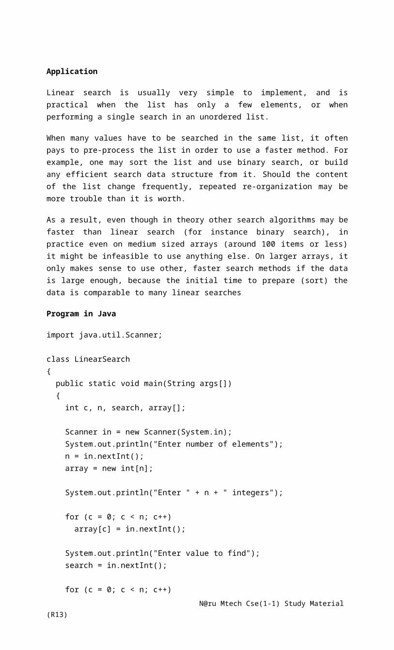
Example:

Java Program for Quick Sort:

import java.util.ArrayList;

public class MyQuickSort {

/** * @param args */ public static void main(String[] args) {

//int[] a = { 1, 23, 45, 2, 8, 134, 9, 4, 2000 }; int a[]={23,44,1,2009,2,88,123,7,999,1040,88}; quickSort(a, 0, a.length - 1); System.out.println(a); ArrayList al = new ArrayList(); }

public static void quickSort(int[] a, int p, int r) { if(p<r) { int q=partition(a,p,r); quickSort(a,p,q); quickSort(a,q+1,r); } }

private static int partition(int[] a, int p, int r) {

int x = a[p]; int i = p-1 ; int j = r+1 ;

while (true) { i++; while ( i< r && a[i] < x)


i++; j--; while (j>p && a[j] > x) j--;

if (i < j) swap(a, i, j); else return j; } }

private static void swap(int[] a, int i, int j) { // TODO Auto-generated method stub int temp = a[i]; a[i] = a[j]; a[j] = temp; }}

7) Describe Merge Sorting Technique?

Merge Sort

• A merge is a common data processing operation:

• Performed on two sequences of data

• Items in both sequences use same compareTo

• Both sequences in ordered of this compareTo

• Goal: Combine the two sorted sequences in one larger sorted sequence

• Merge sort merges longer and longer sequences

Merging two sequences:

1. Access the first item from both sequences

2. While neither sequence is finished

1. Compare the current items of both

2. Copy smaller current item to the output

3. Access next item from that input sequence

3. Copy any remaining from first sequence to output

4. Copy any remaining from second to output


Analysis of Merge

• Two input sequences, total length n elements

• Must move each element to the output

• Merge time is O(n)

• Must store both input and output sequences

• An array cannot be merged in place

• Additional space needed: O(n)

Overview:

• Split array into two halves

• Sort the left half (recursively)

• Sort the right half (recursively)

• Merge the two sorted halves

Example


Program for Merge Sort

public class Mergesort { private int[] numbers; private int[] helper;

private int number;

public void sort(int[] values) { this.numbers = values; number = values.length; this.helper = new int[number]; mergesort(0, number - 1); }

private void mergesort(int low, int high) { // check if low is smaller then high, if not then the array is sorted if (low < high) { // Get the index of the element which is in the middle int middle = low + (high - low) / 2; // Sort the left side of the array mergesort(low, middle); // Sort the right side of the array mergesort(middle + 1, high); // Combine them both merge(low, middle, high); } }

private void merge(int low, int middle, int high) {

// Copy both parts into the helper array for (int i = low; i <= high; i++) { helper[i] = numbers[i]; }

int i = low; int j = middle + 1; int k = low; // Copy the smallest values from either the left or the right side back // to the original array while (i <= middle && j <= high) { if (helper[i] <= helper[j]) { numbers[k] = helper[i]; i++; } else { numbers[k] = helper[j]; j++; } k++; } // Copy the rest of the left side of the array into the target array while (i <= middle) { numbers[k] = helper[i]; k++; i++; }

}}


8) Describe Heap Sorting Technique?

Heapsort

• Merge sort time is O(n log n)

• But requires (temporarily) n extra storage items

• Heapsort

• Works in place: no additional storage

• Offers same O(n log n) performance

• Idea (not quite in-place):

• Insert each element into a priority queue

• Repeatedly remove from priority queue to array

• Array slots go from 0 to n-1

Heap Sort Example:


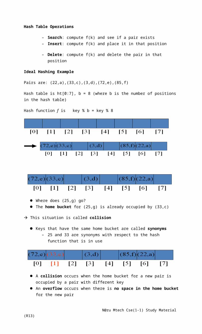
//Source code for Heap Sort public class HeapSort { private static int[] a; private static int n; private static int left; private static int right; private static int largest; public static void buildheap(int []a){ n=a.length-1; for(int i=n/2;i>=0;i–){ maxheap(a,i); } } public static void maxheap(int[] a, int i){ left=2*i; right=2*i+1; if(left <= n && a[left] > a[i]){ largest=left; } else{ largest=i; } if(right <= n && a[right] > a[largest]){ largest=right; } if(largest!=i){ exchange(i,largest); maxheap(a, largest); }


} public static void exchange(int i, int j){ int t=a[i]; a[i]=a[j]; a[j]=t; } public static void sort(int []a0){ a=a0; buildheap(a); for(int i=n;i>0;i–){ exchange(0, i); n=n-1; maxheap(a, 0); } } public static void main(String[] args) { int []a1={4,1,3,2,16,9,10,14,8,7}; sort(a1); for(int i=0;i<a1.length;i++){ System.out.print(a1[i] + " "); } } }

9) Describe Radix Sorting Technique?

Each key is first figuratively dropped into one level of buckets corresponding to the value of the rightmost digit. Each bucket preserves the original order of the keys as the keys are dropped into the bucket. There is a one-to-one correspondence between the number of buckets and the number of values that can be represented by a digit. Then, the process repeats with the next neighbouring digit until there are no more digits to process. In other words:

1. Take the least significant digit (or group of bits, both being examples of radices) of each key.

2. Group the keys based on that digit, but otherwise keep the original order of keys. (This is what makes the LSD radix sort a stable sort).

3. Repeat the grouping process with each more significant digit.

The sort in step 2 is usually done using bucket sort or counting sort, which are efficient in this case since there are usually only a small number of digits.

An example

Original, unsorted list:

170, 45, 75, 90, 802, 2,24, 66

Sorting by least significant digit (1s place) gives:

170, 90, 802, 2, 24, 45, 75, 66

Notice that we keep 802 before 2, because 802 occurred before 2 in the original list, and similarly for pairs 170 & 90 and 45 & 75.


http://en.wikipedia.org/wiki/Counting_sort

http://en.wikipedia.org/wiki/Bucket_sort


http://en.wikipedia.org/wiki/Radix

Sorting by next digit (10s place) gives:

802, 2, 24, 45, 66, 170, 75, 90

Notice that 802 again comes before 2 as 802 comes before 2 in the previous list.

Sorting by most significant digit (100s place) gives:

2, 24, 45, 66, 75, 90, 170, 802

It is important to realize that each of the above steps requires just a single pass over the data, since each item can be placed in its correct bucket without having to be compared with other items.

Some LSD radix sort implementations allocate space for buckets by first counting the number of keys that belong in each bucket before moving keys into those buckets. The number of times that each digit occurs is stored in an array. Consider the previous list of keys viewed in a different way:

170, 045, 075, 090, 002, 024, 802, 066

The first counting pass starts on the least significant digit of each key, producing an array of bucket sizes:

2 (bucket size for digits of 0: 170, 090)


1 (bucket size for digits of 4: 024)



A second counting pass on the next more significant digit of each key will produce an array of bucket sizes:







A third and final counting pass on the most significant digit of each key will produce an array of bucket sizes:

6 (bucket size for digits of 0: 002, 024, 045, 066, 075, 090)



At least one LSD radix sort implementation now counts the number of times that each digit occurs in each column for all columns in a single counting pass. (See the external links section.) Other LSD radix sort implementations allocate space for buckets dynamically as the space is needed.


http://en.wikipedia.org/wiki/Radix_sort#External_links

http://en.wikipedia.org/wiki/Array_data_type

Java Program for RADIX SORT

public class RadixSort{ //----------------------------------------------------------------- // Perform a radix sort on a set of numeric values. //----------------------------------------------------------------- public static void main ( String[] args) { //demonstrate what happens when you violate ADT's basic principles. //Authors code contains only 4-digit integers. If you add a 3-digit integer it "bombs".int[] list = {7843, 4568, 8765, 6543, 7865, 4532, 9987, 3241,

6589, 6622, 211, 2564};

String temp; Integer numObj; int digit, num;

ArrayQueue<Integer>[] digitQueues = (ArrayQueue<Integer>[])(new ArrayQueue[10]); for (int digitVal = 0; digitVal <= 9; digitVal++) digitQueues[digitVal] = new ArrayQueue<Integer>();

// sort the list for (int position=0; position <= 3; position++) { for (int scan=0; scan < list.length; scan++) { temp = String.valueOf (list[scan]); digit = Character.digit (temp.charAt(3-position), 10); digitQueues[digit].enqueue (new Integer(list[scan])); }

// gather numbers back into list num = 0; for (int digitVal = 0; digitVal <= 9; digitVal++) { while (!(digitQueues[digitVal].isEmpty())) { numObj = digitQueues[digitVal].dequeue(); list[num] = numObj.intValue(); num++; } } }

// output the sorted list for (int scan=0; scan < list.length; scan++) System.out.println (list[scan]); }}

10. Draw a table to show comparison of Sorting Algorithms

Comparison of Sortig Algorithms

Sorting Technique Worst Case Average Case

Selection Sort n2 n2

Bubble Sort n2 n2


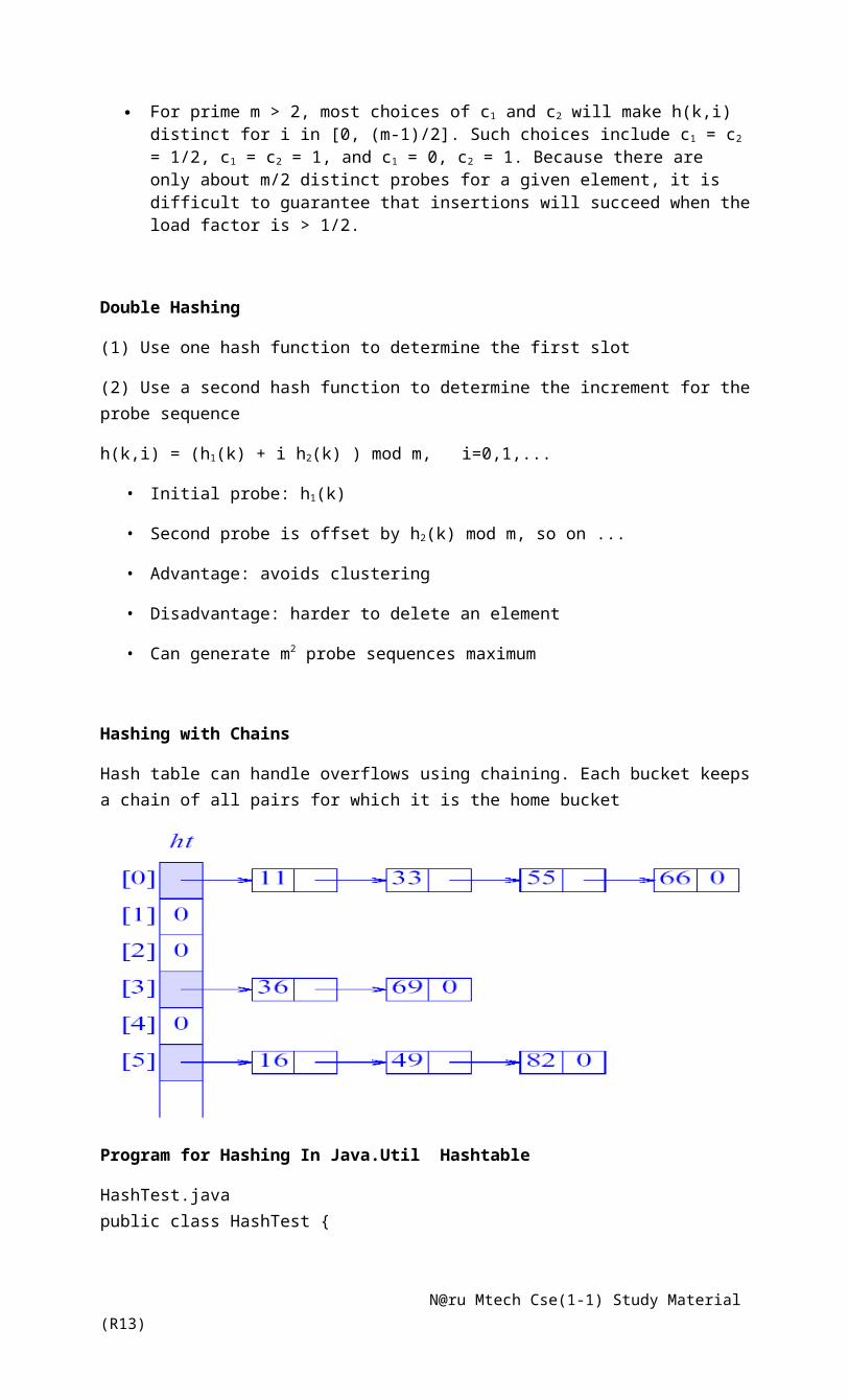
Insertion Sort n2 n2

Merge Sort nlogn nlogn

Quick Sort n2 nlogn

Radix Sort n n

Tree Sort n2 nlogn

Heap Sort nlogn nlogn


1. Implement Heap Sort. [MARCH 2010]

Ans. Refer Unit 3 and Question no. 8

2. Write short notes on Hashing [MARCH 2010]


3. Implement Radix Sort. [SEPT 2010],[NOV 2012]


4. Implement Quick Sort. [SEPT 2010]


5. Explain collision handling schemes [APRIL 2011] [MAY 2012]


6. Implement Quick Sort. [APRIL 2011]



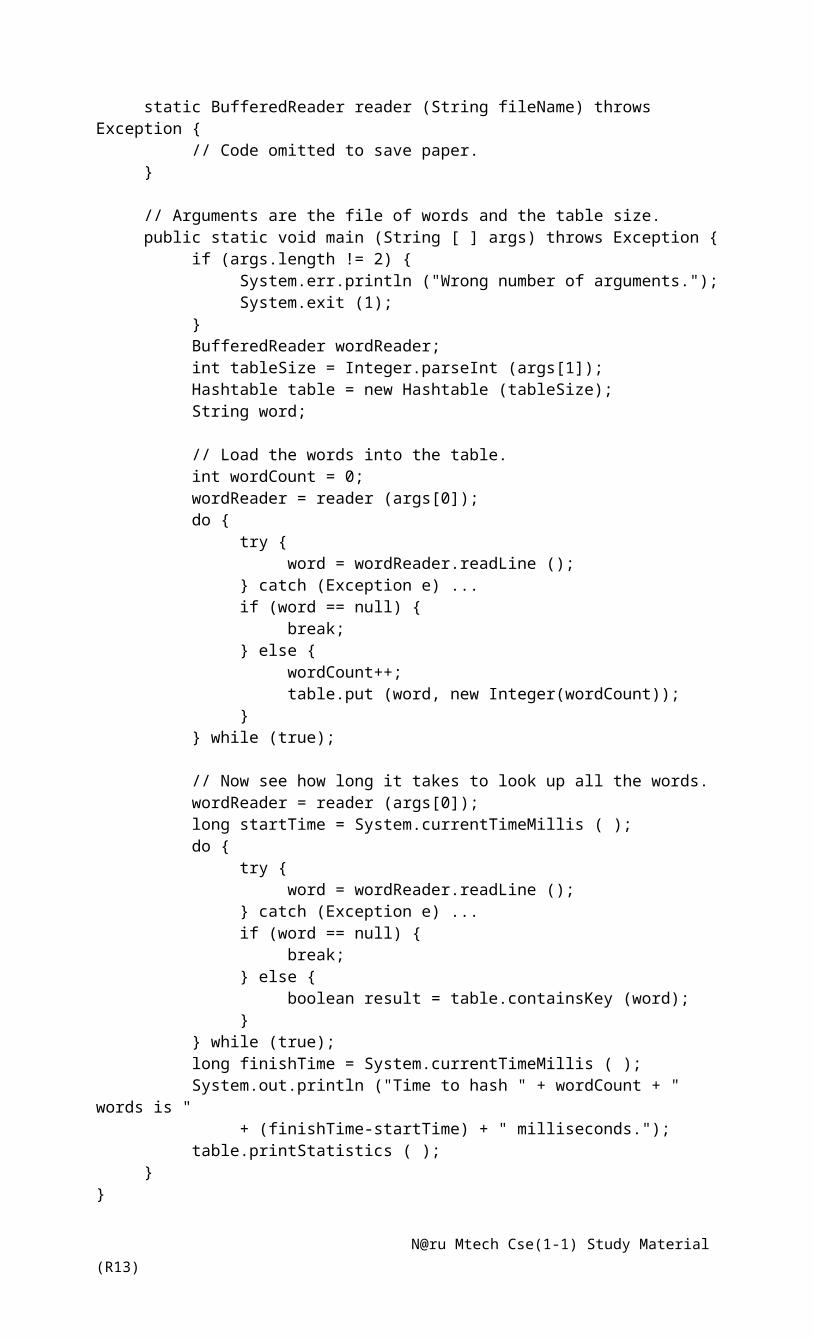
UNIT - 4

Contents:

1) Explain in detail about “Binary Trees”

A binary tree‘t’ is a finite collection of elements. When a binary tree is not empty, it has root element and the remaining elements (if any) are positioned into two binary trees, which are called the left and right sub trees of ‘t’.

The essential difference between a binary tree and a tree are

Each element in a binary tree has exactly two sub trees. Each element in a tree can have any number of sub trees. The sub trees of each element in a binary tree are ordered. That is, we distinguish

between the left and right sub trees. The sub trees are unordered. A binary tree can be empty whereas tree cannot.

Properties

A tree with ‘n’ nodes has exactly ‘n-1’ edges, n>0 Every node except the root has exactly one parent and the root node does not have a

parent. There is exactly one path connecting any two nodes in a tree.

Types of Binary Trees:

Full Binary Tree: The height of a binary tree of height ‘h’ that contains exactly 2h -1 elements is called a full binary tree. The following specified a full binary tree.


Suppose we number the elements in a full binary tree of height ‘h’ using the number through 2h-1. We begin at level1 and go down to level ‘h’. Within the levels are numbered left to right. The elements of the full binary tree of the above fig., have been numbered in this way.

Complete Binary Tree: Now suppose we delete the ‘k’ elements numbered 2h-1, 1 < = i < = 2h. The resulting binary tree is called a complete binary tree is shown below:

Note that full binary tree is special case of complete binary tree. Also, note that the height of complete binary tree contains ‘n’ elements is log 2 (n+1).

Left –Skewed Binary Tree: if the right sub tree is missing in every node of a binary tree, then it is known as left – skewed binary tree.

Right – Skewed Binary Tree: if the list sub tree is missing in every node of a binary tree, then it is known as right – skewed binary tree.

Representation of Binary Trees

Array – Base Representation: the array representation of binary tree utilizes the following property:

Let i, 1 <= i <= n, be the number assigned to an element of a complete binary tree, the following are true:

If i=1, then this is the root of the binary tree, if i>1, then the parent of this element has been assigned the number [ i/2].


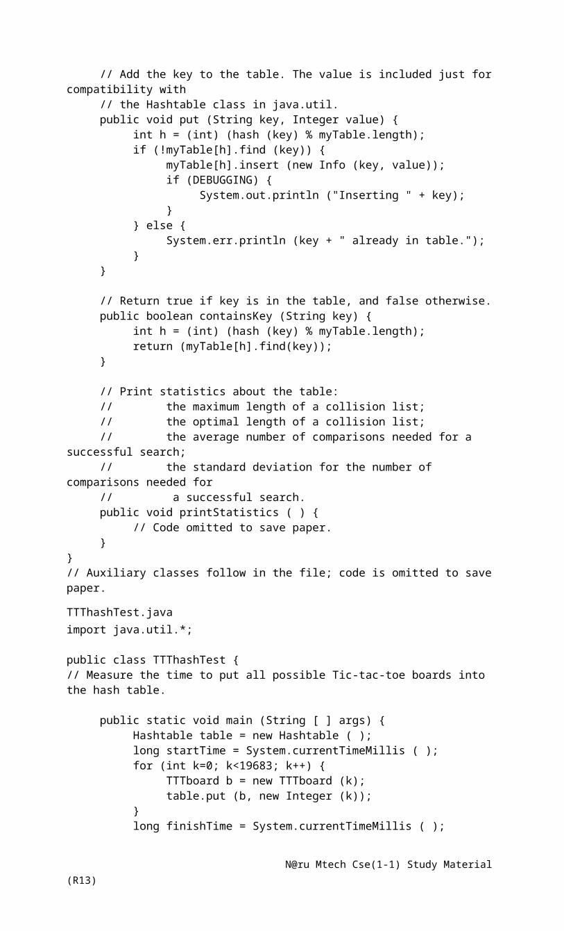
If 2i >1, then this element has no left child. Otherwise, its left child has been assigned the number 2i.

If 2i+1 > n, then this element has no right child. Otherwise its right child has been the number 2i +1.

The binary tree is represented in an array by sorting each element at the array position corresponding to the number assigned to it. The following fig shows the array representations for its binary trees, missing elements are represented by empty boxes.

A binary tree that has ‘n’ elements may require an array of size up to 2n (including position 0) for its representation. This maximum size is needed when each element (except the root) of the n- element binary tree is right child of its parent.

Linked Representation: The most popular way to represent a binary tree is by using links or pointers. A node that has exactly two pointer fields represents each element. Let us call these pointer fields ‘left child’ and ‘right child’. In addition to these two pointer fields, each node has a field named ‘element’.

Each pointer from a parent node to a child node represents an edge drawing of a binary tree. Since an n-elements binary tree has exactly n-1 edges, we are left with 2n-(n+1)= n+1 pointer fields that has no value. These pointer fields are set to NULL. The following fig shows the linked representation of the binary tree is

2) Explain in detail about “Tree Traversals”

There are four common ways to traverse a binary tree

Pre-order In-order Post-order Level-order

Pre-order: in this type, the root is visited first, followed by the left sub tree followed by right sub tree. Thus, the pre order traversal of the sample tree shown below is


Pre-order traversal is: D – B –A – C –F –E –G

Pre-order traversal will be implemented using the following code:

Template <class T>

Void Preorder (binaryTreeNode <T> *t)

{

If(t != NULL)

{

Visit(t);

Preorder( t->leftchild);

Preorder(t->rightchild);

}

}

In-order: the left sub tree is traversed first, followed by the root, and finally by the right sub tree. Thus, the in-order traversal of the sample tree shown earlier would yield the sequence.

A- B – C- D – E – F –G

It will be implemented by the following code

Template <class T>

Void inorder (binaryTreeNode <T> *t)

{

If(t != NULL)

{

inorder( t->leftchild);

visit(t);

inorder(t->rightchild);

}

}

Post-order: the left sub tree is traversed first, followed by the right sub tree and followed by the root. The post order traversal of the sample tree shown earlier would yield sequence

A- C – B- E- G- F – D.


The code to implement this traversal is

Template <class T>

Void Postorder (binaryTreeNode <T> *t)

{

If(t != NULL)

{

Postorder( t->leftchild);

Postorder(t->rightchild);

Visit(t);

}

}

Level-order: elements are visited by level from the top to bottom with in levels, elements are visited from left to right. It is quite difficult to write a recursive function for level order traversal as the correct data structure to use here is a queue and not a stack. Thus the levelorder traversal for the above specified tree is

D- B- E- A- C – F

The code to implement this traversal is:

Template <class T>

Void Levelorder (binarytreenode <T> *t)

{

Arrayqueue <binarytreenode <T> *> q;

While(t != NULL)

{

Visit(t);

If( t->leftchild !=NULL);

q.push(t->leftchild);

if(t->rightchild !=NULL)

q.push(t->rightchild);

try

{

t= q. front();

}

Catch(queue empty)

{

Return;


}

q. pop();

}

}

The time complexity of above specified traversals are O(n).

Java Code for Binary Tree Traversals

public class BinaryTree {

Node root;

public void addNode(int key, String name) {

// Create a new Node and initialize it

Node newNode = new Node(key, name);

// If there is no root this becomes root

if (root == null) {

root = newNode;

} else {

// Set root as the Node we will start

// with as we traverse the tree

Node focusNode = root;

// Future parent for our new Node

Node parent;

while (true) {

// root is the top parent so we start // there


parent = focusNode;

// Check if the new node should go on

// the left side of the parent node

if (key < focusNode.key) {

// Switch focus to the left child

focusNode = focusNode.leftChild;

// If the left child has no children

if (focusNode == null) {

// then place the new node on the left of it

parent.leftChild = newNode; return; // All Done

}

} else { // If we get here put the node on the right

focusNode = focusNode.rightChild;

// If the right child has no children

if (focusNode == null) {

// then place the new node on the right of it

parent.rightChild = newNode;

return; // All Done

}

}

}


}

}

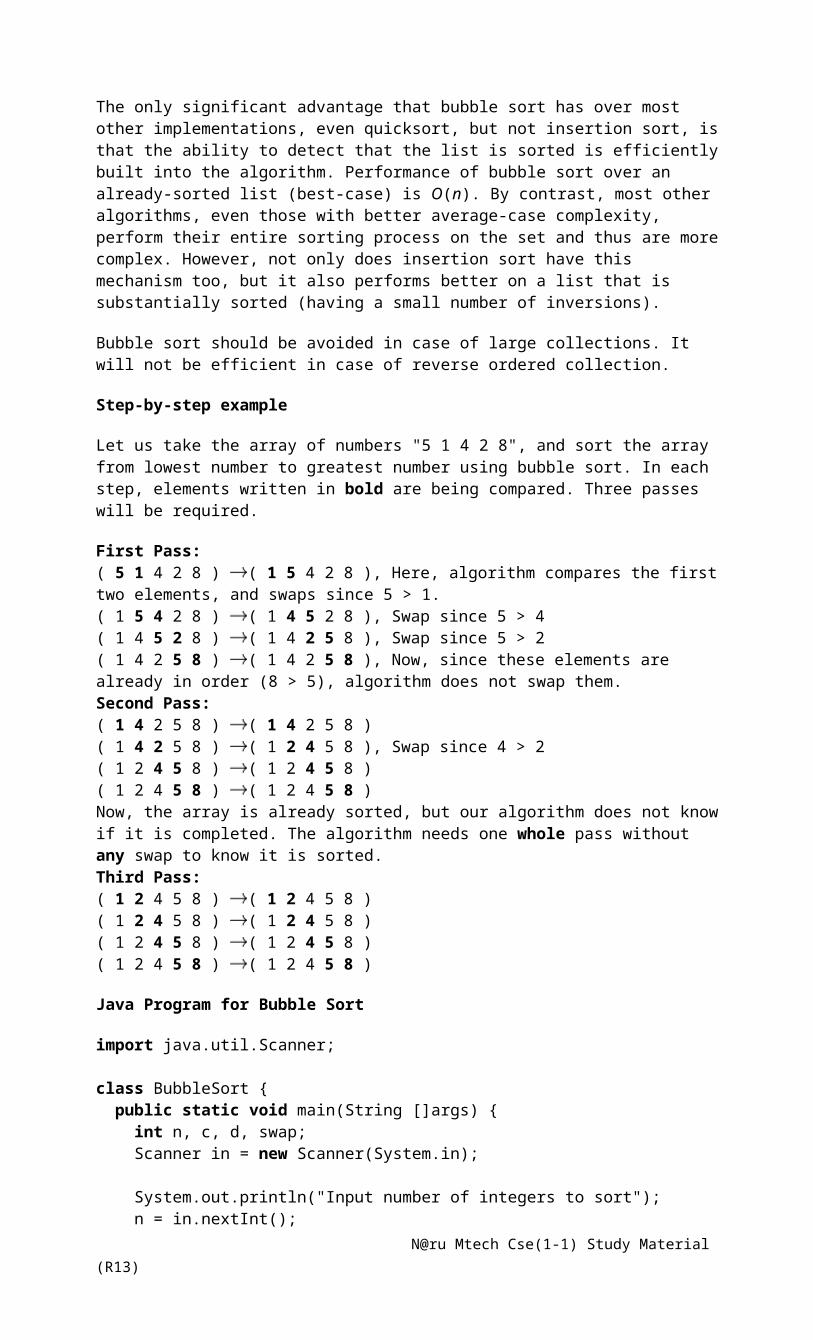
// All nodes are visited in ascending order

// Recursion is used to go to one node and

// then go to its child nodes and so forth

public void inOrderTraverseTree(Node focusNode) {

if (focusNode != null) {

// Traverse the left node

inOrderTraverseTree(focusNode.leftChild);

// Visit the currently focused on node

System.out.println(focusNode);

// Traverse the right node

inOrderTraverseTree(focusNode.rightChild);

}

}

public void preorderTraverseTree(Node focusNode) {



preorderTraverseTree(focusNode.leftChild);

preorderTraverseTree(focusNode.rightChild);

}

}


public void postOrderTraverseTree(Node focusNode) {


postOrderTraverseTree(focusNode.leftChild); postOrderTraverseTree(focusNode.rightChild);


}

}

public Node findNode(int key) {

// Start at the top of the tree

Node focusNode = root;

// While we haven't found the Node

// keep looking

while (focusNode.key != key) {

// If we should search to the left

if (key < focusNode.key) {

// Shift the focus Node to the left child

focusNode = focusNode.leftChild;

} else {

// Shift the focus Node to the right child

focusNode = focusNode.rightChild;

}


// The node wasn't found

if (focusNode == null) return null;

}

return focusNode;

}

public static void main(String[] args) {

BinaryTree theTree = new BinaryTree();

theTree.addNode(50, "Boss");

theTree.addNode(25, "Vice President");

theTree.addNode(15, "Office Manager");

theTree.addNode(30, "Secretary");

theTree.addNode(75, "Sales Manager");

theTree.addNode(85, "Salesman 1");

// Different ways to traverse binary trees

// theTree.inOrderTraverseTree(theTree.root);

// theTree.preorderTraverseTree(theTree.root);

// theTree.postOrderTraverseTree(theTree.root);

// Find the node with key 75

System.out.println("\nNode with the key 75");


System.out.println(theTree.findNode(75));

}}

class Node {

int key; String name;

Node leftChild;

Node rightChild;

Node(int key, String name) {

this.key = key; this.name = name;

}

public String toString() {

return name + " has the key " + key;

/*

* return name + " has the key " + key + "\nLeft Child: " + leftChild + * "\nRight Child: " + rightChild + "\n";

*/

}

}

3) Explain in detail about “Threaded Binary Trees”?

When a binary tree is represented using pointers then pointers to empty sub tree are set to NULL. That is, the left pointer of a node whose left child is an empty sub tree is normally set to NULL. Similarly, the right pointer of a node whose right child is an empty sub tree is also set to NULL. Thus, a large number of pointers are set to NULL. These NULL pointers could be used in different and more effective way.


Assume that the left pointer of a node ‘n’ is set to NULL as the left child of ‘n’ is an empty sub tree. Then the left pointer of ‘n’ can be set to point to the in order predecessor of ‘n’. Similarly, if the right child of a node ‘m’ is empty then the right pointer of ‘m’ is empty then the right pointer of ‘m’ can be set to point to in order successor of ‘m’. the following fig shows a threaded binary tree, lines with arrows represents threads.

In the above fig., links with arrows heads indicate links leading to in order successors while other lines denote the usual links in a binary tree. Note that link with arrows and the normal links indicate different relationship between nodes and the links are no longer used to describe only ‘parent-child’ relationship. Consequently, it must be understood whether the left or right link of node ‘n’ is

leading to its children or to in order predecessor of ‘n’ or to the in order successor of ‘n’. Two flags, left flag and right flag are used per node to indicate the type of its left or right links. If left flag of a node is ‘0’ then its left link leads to the left sub tree of ‘n’. Otherwise, the left link leads to the in order predecessor of ‘n’. Similarly, if the right flag of a node ‘n’ is ‘0’ then the right link leads to the right sub

tree of ‘n’, otherwise the right link leads to the in-order successor ‘n’. The left and right link leading to in-order predecessors or successors are called threaded to distinguish them from the conventional links of a binary tree. The links are used as threads only they would have a pointed to empty sub-tree on a non-threaded binary tree. Every node in a threaded binary tree must contain the flags, to indicate whether its left and right pointers are threads. Hence the structure of a node in such trees contain two more fields: ‘data’, ‘left’ and ‘right’ as shown in the following fig.,

The traversal sequence of the nodes of the above specified tree is

In-order: D- J- H- K- B- E- A- F- C- I- G

Pre-order: A- B- D- H- J- K- E- C- F- G- I

Post-order: D- J- K- H- E- B- F- I- G- C- A


4) Explain in detail about “Graphs”

A graph is a collection of vertices or nodes, connected by a collection of edges. Formally G is a finite set defined as (V,E).

where

V- set of Vertices

E- set of Edges

G = ( V, E)

V= { 1, 2, 3, 4, 5}

E= { e1, e2, e3, e4, e5, e6}

Applications:

• These are used in communication and transportation networks.

• These are used in shape description in computer – aided design and geometric information system and scheduling system.

Directed Graph (Diagraph)

A graph G consists of finite set V – called the vertices or nodes, E- set of ordered pairs, called edges of G. self loops are allowed in diagraph.

’

Representation of Graphs:

There are two commonly used methods of representing the graphs

Adjacency Matrix:

In this method the graph can be represented by using matrix of n*n such that

A[i] [j] = 1 if (I, j) is an edge else 0

If the diagraph has weights we can store the weights in the matrix.


Adjacency list:

In this method graph can be represented using linked list. In this method there is an array of linked list for each vertex V in the graph. If the edge have weights then these weights can be stored in the linked list elements.

5) Explain in detail about “Graph Searching Algorithms”

•A systematically follow up of the edges the graph in order to visit the vertices of the graph is called graph searching.

•There are two basic searching algorithms:

i) Breadth –First –Searchii) Depth –First –Search

The difference between those is in order in which they explore the un visited edges of the graph.

Breadth –first –Search

BFS follows the following rules:

•Select an unvisited node V, visit it, have it be the root in a BFS tree being formed. Its level is called the current level.

•For each node x in the current level, in the order in which the level nodes were visited, visit all unvisited neighbors of x. the newly visited nodes from this level from a new level. This new level becomes the next current level.

•Repeat step2 for all unvisited vertices.

•Repeat from step1 until no more vertices remaining.

Ex: consider the following graph

BFS Sequence is A-B-C-D-E-F-G-H

Java Program for BFS

import java.io.*;

class bfs1

{

public static void main(String args[]) throws IOException

{


int i,n,j,k;

System.out.println("No. of vertices :") ;

BufferedReader br= new BufferedReader (new InputStreamReader(System.in));

n =Integer.parseInt(br.readLine());

int q[] = new int[10];

int m[] = new int[10];

int a[][] = new int[10][10];

for (i=0; i<10; i++)

{

m[i] = 0;

}

System.out.println("\n\nEnter 1 if edge is present, 0 if not");

for (i=0; i<n; i++)

{

System.out.println("\n");

for (j=i; j<n; j++)

{

System.out.println("Edge between " + (i+1) + " and " + (j+1)+ ":" );

a[i][j]=Integer.parseInt(br.readLine());

a[j][i]=a[i][j];

}

a[i][i]=0;

}

System.out.println("\nOrder of accessed nodes : \n");

q[0] = 0; m[0] = 1;

int u;

int node=1;

int beg1=1, beg=0;

while(node>0)

{


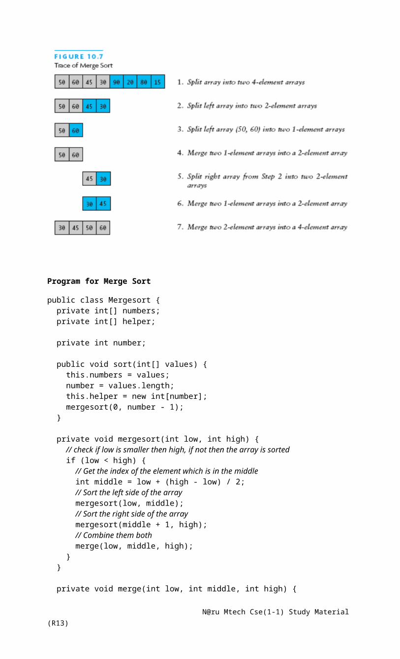
u=q[beg];beg++;

System.out.println(" " +(u+1));

node--;

for(j=0;j<n;j++)

{

if(a[u][j]==1)

{

if(m[j]==0)

{

m[j]=1;

q[beg1]=j;

node++;

beg1++;

}

}

}

}

}

}

DepthFirstSearch

It begins from then a particular vertex, then one of its child is visited and then the child of child is visited. This process continuous until we reach the bottom of the graph.

Ex: consider the following graph


The DFS Sequence is : A-B-E-F-C-D-G-H

Java Program for DFS

import java.io.*;

class dfs

{

static void dfs(int a[][], int m[], int i, int n)

{

int j;

System.out.println("\t" + (i+1));

m[i] = 1;

for(j=0; j<n; j++)

if(a[i][j]==1 && m[j]==0)

dfs(a,m,j,n);

}

public static void main(String args[]) throws IOException

{

int n, i, j;

System.out.println("No. of vertices : ");

BufferedReader br= new BufferedReader (new InputStreamReader(System.in))

n =Integer.parseInt(br.readLine());

int m[]= new int[n];

int a[][] = new int[n][n];

for (i=0; i<n; i++)


{

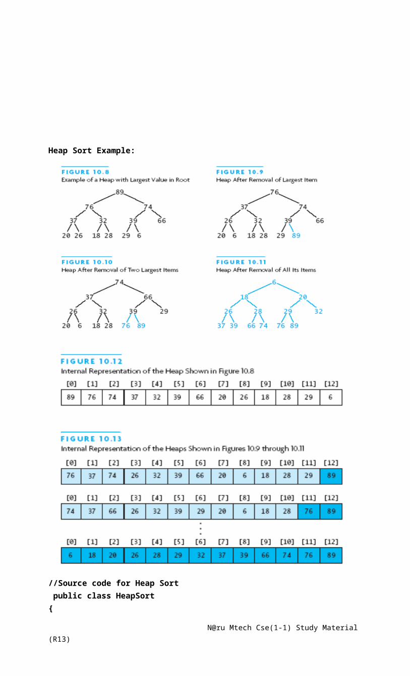
m[i] = 0;

}

System.out.println("\n\nEnter 1 if edge is present, 0 if not");

for (i=0; i<n; i++)

{

System.out.println("\n");

for (j=i; j<n; j++)

{

System.out.println("Edge between " + (i+1) + " and " + (j+1)+ " : ");

a[i][j] =Integer.parseInt(br.readLine());

a[j][i]=a[i][j];

}

a[i][i] = 0;

}

System.out.println("\nOrder of accessed nodes : \n");

for (i=0; i<n; i++)

if (m[i]==0)

dfs(a,m,i,n);

}

}

6) Explain in detail about “Spanning Trees”

Minimum Spanning Trees:

A minimum spanning tree connects all nodes in a given graph

A MST must be a connected and undirected graph

A MST can have weighted edges

Multiple MSTs can exist within a given undirected graph

Multiple MSTs can be generated depending on which algorithm is used

If you wish to have an MST start at a specific node


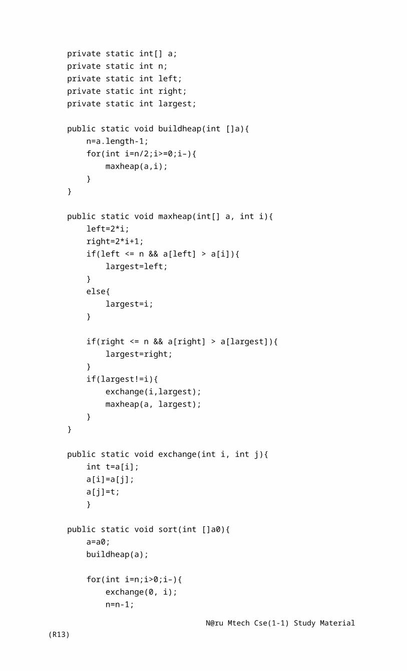
However, if there are weighted edges and all weighted edges are unique, only one MST will exist

Real Life Application of a MST

A cable TV company is laying cable in a new neighborhood. If it is constrained to bury the cable only along certain paths, then there would be a graph representing which points are connected by those paths. Some of those paths might be more expensive, because they are longer, or require the cable to be buried deeper; these paths would be represented by edges with larger weights. A minimum spanning tree would be the network with the lowest total cost.

Kruskal’s Algorithm

Created in 1957 by Joseph Kruskal

Finds the MST by taking the smallest weight in the graph and connecting the two nodes and repeating until all nodes are connected to just one tree

This is done by creating a priority queue using the weights as keys

Each node starts off as it’s own tree

While the queue is not empty, if the edge retrieved connects two trees, connect them, if not, discard it

Once the queue is empty, you are left with the minimum spanning tree

An example for Kruskal’s Algorithm

Step 1:

Step 2:


Step 3

Step 4


Step 5

Step 6


Step 7

7) Explain in detail about “Dijkstra’s Algorithm”

Single-Source Shortest Path Problem

Single-Source Shortest Path Problem - The problem of finding shortest paths from a source vertex v to all other vertices in the graph.


Dijkstra's algorithm - is a solution to the single-source shortest path problem in graph theory.

Works on both directed and undirected graphs. However, all edges must have nonnegative weights.

Approach: Greedy

Input: Weighted graph G={E,V} and source vertex v∈V, such that all edge weights are nonnegative

Output: Lengths of shortest paths (or the shortest paths themselves) from a given source vertex

v∈V to all other vertices

Dijkstra's algorithm – Pseudocode

dist[s] ←0 (distance to source vertex is zero)

for all v ∈ V–{s} do dist[v] ←∞ (set all other distances to infinity)

S←∅ (S, the set of visited vertices is initially empty) Q←V (Q, the queue initially contains all vertices)

while Q ≠∅ (while the queue is not empty) do u ← mindistance(Q,dist) (select the element of Q with the min. distance)

S←S∪{u} (add u to list of visited vertices)

for all v ∈ neighbors[u] do if dist[v] > dist[u] + w(u, v) (if new shortest path found) then d[v] ←d[u] + w(u, v) (set new value of shortest path)

(if desired, add traceback code)

return dist

An Example:

Step 1:

Step 2:


Step 3:

Step 4:

Step 5:


Step 6:

Step 7:

Step 8:


Implementations and Running Times

The simplest implementation is to store vertices in an array or linked list. This will produce a running time of

O(|V|^2 + |E|)

For sparse graphs, or graphs with very few edges and many nodes, it can be implemented more efficiently storing the graph in an adjacency list using a binary heap or priority queue. This will produce a running time of

O((|E|+|V|) log |V|)

As with all greedy algorithms, we need to make sure that it is a correct algorithm (e.g., it always returns the right solution if it is given correct input).


1. Write about BFS Graph Traversal [SEPT 2010] [MARCH 2010]

Ans: Refer Unit 4 Question no.5

2. Implement Kruskal’s Algorithm for Minimum Cost Spanning Trees. [SEPT 2010]


3. Discuss graph traversal techniques. [NOV 2011] [MAY 2012]


4. Explain the properties of a binary tree. [APRIL 2011]



mtech adsa final 2nd jan 1,2,3,4

Documents

java code

data structureslinear

linear data structures

advanced data structures

classic data structures

binary trees terminology

comparison of search

insertion sort