msc in big data analytics department of computer...

MSc in Big Data Analytics

Department of Computer Science

RKMVERI, Belur Campus

Program Outcomes

Program Specific Outcomes

Course Outcomes

1

Program outcomes

• Inculcate critical thinking to carry out scientific investigation objectively without being biased with

preconceived notions.

• Equip the student with skills to analyze problems, formulate an hypothesis, evaluate and validate

results, and draw reasonable conclusions thereof.

• Prepare students for pursuing research or careers in industry in mathematical sciences and allied fields

• Imbibe effective scientific and/or technical communication in both oral and writing.

• Continue to acquire relevant knowledge and skills appropriate to professional activities and demonstrate

highest standards of ethical issues in mathematical sciences.

• Create awareness to become an enlightened citizen with commitment to deliver ones responsibilities

within the scope of bestowed rights and privileges.

Program Specific Outcomes

• Basic understanding of statistical methods, probability, mathematical foundations, and computing

methods relevant to data analytics.

• Knowledge about storage, organization, and manipulation of structured data.

• Understand the challenges associated with big data computing.

• Training in contemporary big data technologies

• Understanding about the analytics chain beginning with problem identification and translation, fol-

lowed by model building and validation with the aim of knowledge discovery in the given domain.

• Applying dimensionality reduction techniques in finding patterns/features/factors in big data.

• Estimation of various statistics from stored and/or streaming data in the iterative process of model

selection and model building.

• Future event prediction associated with a degree of uncertainty.

• Modelling optimization techniques such as linear programming, non-linear programming, transporta-

tion techniques in various problem domains such as marketing and supply chain management.

• Interpret analytical models to make better business decisions.

2

DA102

Basic Statistics

Time: TBAPlace: IH402 & Bhaskara Lab

Dr. Sudipta Das

[email protected]

Office: IH404, Prajnabhavan, RKMVERI, BelurOffice Hours: 11 pm—12 noon, 3 pm—4 pm(+91) 99039 73750

Course Description: DA102 is going to provide an introduction to some basic statistical methods foranalysis of categorical and continuous data. Students will also learn to make practical use of the statisticalcomputer package R.

Prerequisite(s): NANote(s): Syllabus changes yearly and may be modified during the term itself, depending on the circum-stances. However, students will be evaluated only on the basis of topics covered in the course.Course url:Credit Hours: 4

Text(s):

Statistics;

David Freedman, Pobert Pisani and Roger Purves

The visual display of Quantitative Information;

Edward Tufte

Mathematical Statistics with Applications;

Kandethody M. Ramachandran and ChrisP.Tsokos

Course Objectives:

Knowledge acquired: Students will get to know(1) fundamental statistical concepts and some of their basic applications in real world.(2) organizing, managing, and presenting data,(3) how to use a wide variety of specific statistical methods, and,(4) computer programming in R.

Skills gained: The students will be able to(1) apply technologies in organizing different types of data,(2) present results effectively by making appropriate displays, summaries, and tables of data,(3) perform simple statistical analyses using R(4) analyze the data and come up with correct interpretations and relevant conclusions.

1

Course Outline (tentative) and Syllabus:The weekly coverage might change as it depends on the progress of the class. However, you must keep upwith the reading assignments. Each week assumes 4 hour lectures. Quizzes will be unannounced.

Week Content

Week 1 Introduction, Types of Data, Data Collection, Introduction to R, R fundamentals, Arith-metic with R

Week 2Tabular Representation: Frequency Tables, Numerical Data Handling, Vectors, Matrices,Categorical Data Handling

Week 3 Data frames, Lists, R programming, Conditionals and Control Flow, Loops, Functions

Week 4Graphical Representation: Bar diagram, Pie-chart, Histogram, Data Visualization in R,Basis R graphics, Different plot types, Plot customizations

Week 5Descriptive Numerical Measures:- Measures of Central Tendency, Measures of Variability,Measure of Skewness, KurtosisQuiz 1

Week 6 Descriptive Statistics using R:- Exploring Categorical Data, Exploring Numerical Data

Week 7 Numerical Summaries, Box and Whiskers PlotWeek 8 Problem Session, Review for Midterm exam

Week 9 Concept of sample and population, Empirical distribution, Fitting probability distribution

Week 10 Goodness of fit, Distribution fitting in R

Week 11Analysis of bivariate data:- Correlation, Scatter plotRepresenting bivariate data in R

Week 12 Simple linear regression

Week 13Linear Regression in RQuiz 2

Week 14 Two-way contingency tables, Measures of association, Testing for dependence

Week 15 Problem Session, Review for Final Exam

2

DA321 Modeling for Operations Management

InstructorSudeep Mallick, [email protected]

Course Description:DA321 deals with the topics in modelling techniques for accomplishingoperations management tasks for business. In particular, the course will coveradvanced techniques of operations research and modelling along with theirapplications in various business domains with a special focus on supply chainmanagement and supply chain analytics.

Prerequisite(s): Basic course in Operations Research covering LinearProgramming fundamentals.Credit Hours: 4

Text(s):

Operations Research, seventh revised edition (2014)P K Gupta and D S HiraISBN: 81-219-0218-9

Introduction to Operations Research, eighth edition Frederick S. Hillier & Gerald J. Lieberman ISBN: 0-07-252744-7

Operations Research: An Introduction, ninth editionHamdy A. TahaISBN: 978-93-325-1822-3

AMPL: A Modeling Language for Mathematical Programming, second Editionwww.ampl.com

Course Objectives:

Knowledge acquired:1. Different operations research modelling techniques.2. Application of the modelling techniques in business domains.3. Hands-on implementation of the models using computer software such as

MS-EXCEL, CPLEX solvers.

Skills acquired: Students will be able to1. apply the appropriate operations research technique to formulate

mathematical models of the business problem2. implement and evaluate alternative models of the problem in computer

softwareGrade Distribution:Assignments 20%, Internal Test 20%, Mid-term exam 30%, Final exam 30%Course Outline (tentative) and Syllabus:

http://www.ampl.com/

mailto:[email protected]

Week ContentWeek 1 Advanced Linear Programming: Duality theory, Dual Simplex

method Reading assignment: Chapter 6, GH / Chapter 4, HT

Week 2 Lab session on Linear Programming and Sensitivity Analysis withAMPL (CPLEX solver)

Lab assignment 1, Reading assignment: AMPL manualWeek 3 Supply chain management modelling: supply chain management

definition, modelling, production planning decisions Reading assignment: Instructor notes

Week 4 Lab session on modelling aggregate planning problemsWeek 5 Transportation problem: transportation model, solution

techniques, variations. Reading assignment: Chapter 3, GH / Chapter 5, HT Transportation problem Lab sessions Lab instructions: Instructor notes

Week 6 Multi-stage transportation problem: formulation, solutiontechniques, truck allocation problem, Traveling SalesmanProblem, vehicle routing problem

Reading assignment: Instructor notes Internal test 1

Week 7 Assignment problem: assignment, solution techniques Reading assignment: Chapter 4, GH / Chapter 5. HT Lab assignment 2

Week 8 Integer programming: problem formulation and solutiontechniques

Reading assignment: Chapter 6, GH / Chapter 9, HT Review for Midterm Exam

Week 9 Non-linear Programming: problem formulation and solutiontechniques

Reading assignment: Chapter 16, GH / Chapter 21, HT Lab assignment 3

Week 10 Inventory management: deterministic inventory models, cycleinventory models

Reading assignment: Chapter 12, GH / Chapter 13, HT Internal test 2

Week 11 Inventory management: stochastic inventory models, safetystock models

Reading assignment: Chapter 12, GH / Chapter 13, HT Lab session: Inventory management modeling Reading assignment: Instructor notes

Week 12 Lab Session: Supply chain management beer gameWeek 13 Queueing theory: pure birth and death models

Reading assignment: Chapter 10, GH / Chapter 18, HT Reading assignment: Chapter 10, GH / Chapter 18, HT

Week 14 Queueing theory: general poisson model, specialised poissonqueues

Lab session: queueing theory Reading assignment: Chapter 10, GH / Chapter 18, HT Lab assignment 4

Week 15 Queueing theory: queueing decision models Reading assignment: Chapter 10, GH / Chapter 18, HT

DA205 Data Mining

Instructor: Prof. Aditya Bagchi

Course Description: The quantity and variety of online data is increasing very rapidly. The datamining process includes data selection and cleaning, machine learning techniques to “learn” knowledge thatis “hidden” in data, and the reporting and visualization of the resulting knowledge. This course will coverthese issues.

Prerequisite(s): First course in DBMS,Credit Hours: 2

Text(s):

• Data Mining Concepts and techniques, J. Han and M. Kamber, Morgan Kaufmann.

• Mining of Massive datasets, A. Rajaraman, J. Leskovec, J.D. Ullman

• Mining the WEB, S. Chakrabarti, Morgan Kaufmann.

Course Objectives:

Knowledge acquired: At the finish of this course, students will be quite empowered and will know(1) standard data mining problems and associated algorithms.(2) how to apply and implement standard algorithms in similar problem.

Competence Developed: The student will be able to(1) Understand a data environment, extract relevant features and identify necessary algorithms forrequired analysis.(2) Accumulation, extraction and analysis of Social network data.

Course Outline (tentative) and Syllabus: The weekly coverage might change as it depends onthe progress of the class. However, you must keep up with the reading assignments. Each week assumes 4hour lectures.

1. Introduction to Data Mining concept, Data Cleaning, transformation, reduction and summarization.(1 lecture = 2 hours)

2. Data Integration - Multi and federated database design, Data Warehouse concept and architecture. (2lectures = 4 hours)

3. Online Analytical Processing and Data Cube. (2 lectures =4 Hours)

4. Mining frequent patterns and association of items, Apriori algorithm with fixed and variable support,improvements over Apriori method - Hash-based method, Transaction reduction method, Partitioningtechnique, Dynamic itemset counting method. (2 Lectures = 4 Hours)

5. Frequent Pattern growth and generation of FP-tree, Mining closed itemsets. (1 Lecture = 2 Hours)

6. Multilevel Association rule, Association rules with constraints, discretization of data and associationrule clustering system. (1 Lecture = 2 Hours)

7. Association mining to Correlation analysis. (1 Lecture = 2 Hours)

8. Mining time-series and sequence data. (2 Lectures = 4 Hours)

9. Finding similar items and functions for distance measures. (4 Lectures = 8 Hours)

10. Recommendation system, content based and collaborative filtering methods. (5 Lectures = 10 Hours)

11. Graph mining and social network analysis. (5 Lectures = 10 Hours)

1

DA220Machine Learning

Instructor: Tanmay Basu

Course Description: DA220 deals with topics in supervised and unsupervised learning methodolo-gies. In particular, the course will cover different advanced models of data classification and clusteringtechniques, their merits and limitations, different use cases and applications of these methods. Moreover,different advanced unsupervised and supervised feature engineering schemes to improve the performance ofthe learning techniques will be discussed.

Prerequisite(s): (1) Linear Algebra and (2) Probability and Stochastic processesCredit Hours: 4

Text(s):

Introduction to Machine Learning E. Alpaydin ISBN: 978-0262-32573-8The Elements of Statistical Learning J. H. Friedman, R. Tibshirani, and T. Hastie ISBN: 978-0387-84884-6Pattern Recognition S. Theodoridis and K. Koutroumbas ISBN: 0-12-685875-6Pattern Classification R. O. Duda, P. E. Hart and D. G. Stork ISBN: 978-0-471-05669-0Introduction to Information Retrieval C. D. Manning, P. Raghavan and H. Schutze ISBN: 978-0-521-86571-5

Course Objectives:

Knowledge Acquired:

1) The background and working principles of various supervised learning techniques viz., linearregression, logistic regression, bayes and naive bayes classifiers, support vector machine etc. andtheir applications.

2) The importance of cross validation to optimize the parameters of a classifier.

3) The idea of different kinds of clustering techniques e.g., k-means, k-medoid, single-linkage, DB-SCAN algorithms and their merits and demerits.

4) The significance of feature engineering to improve the performance of the learning techniques andoverview of various supervised and unsupervised feature engineering techniques.

5) The essence of different methods e.g., precision, recall etc. to evaluate the performance of themachine learning techniques.

Skills Gained: The students will be able to

1) pre-process and analyze the characteristics of different types of standard data,

2) work on scikit-learn, a standard machine learning library,

3) evaluate the performance of different machine learning techniques for a particular application andvalidate the significance of the results obtained.

Competence Developed:

1) Build skills to implement different classification and clustering techniques as per requirement toextract valuable information from any type of data set.

2) Can train a classifier on an unknown data set to optimize its performance

3) Develop novel solutions to identify significant features in data e.g., identify the feedback of po-tential buyers over online markets to increase the popularity of different products.

Evaluation:Assignments 50% Midterm Exam 25% Endterm Exam 25%

Course Outline (tentative) and Syllabus:The weekly coverage might change as it depends on the progress of the class. However, you must keep upwith the reading assignments. Each week assumes 4 hour lectures.

1

Week Contents

Week 1

• Overview of machine learning: idea of supervised and unsupervised learning, regres-sion vs classification, concept of training and test set, classification vs clustering andsignificance of feature engineering

• Linear regression: least square and least mean square methods

Week 2• Bayes decision rule: bayes theorem, bayes classifier and error rate of bayes classifier• Minimum distance classifier and linear discriminant function as derived from Bayes

decision rule

Week 3• Naive bayes classifier: gaussian model, multinomial model, bernoulli model• k-Nearest Neighbor (kNN) decision rule: idea of kNN classifier, distance weighted kNN

decision rule and other variations of kNN decision rule

Week 4• Perceptron learning algorithm: incremental and batch version, proof of convergence• XOR problem, two layer perceptrons to resolve XOR problem, introduction to multi-

layer perceptrons

Week 5 • Discussion on different aspects of linear discriminant functions for data classification• Logistic regression and maximum margin classifier

Week 6 • Support vector machine (SVM): hard margin• Soft margin SVM classifier

Week 7 • Cross validation and parameter tuning• Different techniques to evaluate the classifiers e.g., precision, recall and f-measure

Week 8• The basics to work with Scikit-learn: a machine learning repository in python• How to implement different classifiers in scikit-learn, tune the parameters and evaluate

the performance

Week 9• Text classification(case study for data classification): overview of text data, stemming

and stopword removal, tf-idf weighting scheme and n-gram approach.• How to work with text data in scikit-learn

Week 10

• Assignment 2: Evaluate the performance of different classifiers to classify a newswiree.g., Reuters-21578.

• Review for midterm exam• Data clustering: overview, cluster validity index

Week 11 • Partitional clustering methods: k-means, bisecting k-means• k-medoid, buckshot clustering techniques

Week 12• Hierarchical clustering techniques: single linkage, average linkage and group average

hierarchical clustering algorithms• Density based clustering technique e.g., DBSCAN

Week 13• Feature engineering: overview of feature selection, supervised and unsupervised feature

selection techniques• Overview of principal component analysis for feature extraction

Week 14• How to work with Wordnet, an English lexical database• Sentiment analysis (case study for data clustering): overview, description of a data set

of interest for sentiment identification, sentiment analysis using Wordnet

Week 15• Assignment 2: Sentiment analysis from short message texts• Practice class for the second assignment• Review for endterm exam

2

DA104 Probability and Stochastic Processes

Instructor

Dr. Arijit Chakraborty (ISI Kolkata)

Course Description:

DA104 deals with technologies and engineering solutions for enabling big data processing andanalytics . More specifically, it deals with the tools for data processing, data management andprogramming in the distributed programming paradigm using techniques of MapReduce programming,NoSQL distributed databases, streaming data processing, data injestion, graph processing anddistributed machine learning for big data use cases.

Prerequisite(s): (1) Basic knowledge of python and Java programming languages (2) Tabular dataprocessing / SQL queries. (3) Basic knowledge of common machine learning algorithms.Credit Hours: 4

Text(s):

1. Introduction to time series analysis; PJ Brockwell and RA Davis2. Time Series Analysis and Its Applications; Robert H. Shumway and David S. Stoffer 3. Introduction to Statistical time series; WA Fuller4. A first course in Probability, Sheldon Ross, Pearson Education, 20105. Time Series Analysis; Wilfredo Palma6. P. G. Hoel, S. C. Port and C. J. Stone: Introduction to Probability Theory, University Book

Stall/Houghton Mifflin, New Delhi/New York, 1998/1971.

Syllabus

1. Basic Probabilitya. Introductionb. Sample Spacesc. Probability Measuresd. Computing Probabilities: Counting Methods i. The Multiplication Principle ii. Permutations and Combinationse. Conditional Probabilityf. Independence

2. Random Variablesa. Discrete Random Variables i. Bernoulli Random Variables ii. The Binomial Distribution iii. Geometric and Negative Binomial Distributions iv. The Hypergeometric Distribution v. The Poisson Distributionb. Continuous Random Variables

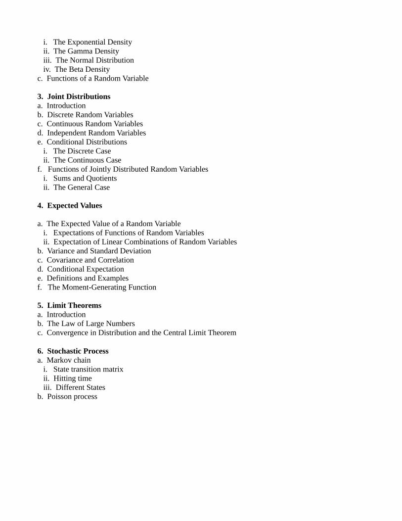
i. The Exponential Density ii. The Gamma Density iii. The Normal Distribution iv. The Beta Densityc. Functions of a Random Variable

3. Joint Distributionsa. Introductionb. Discrete Random Variablesc. Continuous Random Variablesd. Independent Random Variablese. Conditional Distributions i. The Discrete Case ii. The Continuous Casef. Functions of Jointly Distributed Random Variables i. Sums and Quotients ii. The General Case

4. Expected Values

a. The Expected Value of a Random Variable i. Expectations of Functions of Random Variables ii. Expectation of Linear Combinations of Random Variablesb. Variance and Standard Deviationc. Covariance and Correlationd. Conditional Expectatione. Definitions and Examplesf. The Moment-Generating Function

5. Limit Theoremsa. Introductionb. The Law of Large Numbersc. Convergence in Distribution and the Central Limit Theorem

6. Stochastic Processa. Markov chain i. State transition matrix ii. Hitting time iii. Different Statesb. Poisson process

DA230Enabling Technologies for Big Data Computing

InstructorSudeep Mallick, [email protected]

Course Description:DA230 deals with technologies and engineering solutions for enabling big dataprocessing and analytics . More specifically, it deals with the tools for dataprocessing, data management and programming in the distributed programmingparadigm using techniques of MapReduce programming, NoSQL distributeddatabases, streaming data processing, data injestion, graph processing anddistributed machine learning for big data use cases.

Prerequisite(s): (1) Basic knowledge of python and Java programminglanguages (2) Tabular data processing / SQL queries. (3) Basic knowledge ofcommon machine learning algorithms.Credit Hours: 4

Text(s):

Hadoop: The Definitive Guide, fourth editionTom WhiteISBN: 978-1-491-90163-2

Hadoop in Action, edition: 2011 Chuck LamISBN: 978-1-935-18219-1

Spark in Action, edition: 2017Petar Zecevic & Marko BonaciISBN: 978-93-5119-948-9

Data-Intensive Text Processing with MapReduce, edition: 2010Jimmy Lin & Chris DyerISBN: 978-1-608-45342-9

mailto:[email protected]

Course Outline (tentative) and Syllabus:The weekly coverage might change as it depends on the progress of the class.Each week assumes 4 hour lectures.

Week ContentWeek 1 Big data computing paradigm and Hadoop: big data, hadoop

architecture Reading assignment: Chapter 1, LD & Chapter 1, TW Lab: setting up Hadoop platform in standalone mode

Week 2 Hadoop MapReduce (MR): Lab session with simple MR algorithmsin Hadoop standalone mode

Reading assignment: Chapter 2, LD & Chapter 2, TWWeek 3 Hadoop Distributed File System (HDFS), YARN and MR

architecture, daemons, serialization concept, command lineparameters: Lab session

Reading assignment: Chapter 3-5 & 7, TWWeek 4 Implementing algorithms in MR - joins, sort, text processing, etc.:

Lab session Reading assignment: Chapter 3, LD & Chapter 7, TW Lab assignment 1

Week 5 Hadoop operations in Cluster Mode, Hadoop on AWS Cloud: Labsession

Reading assignment: Instructor notesWeek 6 Understanding NoSQL using Pig: Lab Session

Reading assignment: Chapter 16, TW Lab assignment 2

Week 7 Introduction to Apache Spark platform and architecture, RDD, Reading assignment: Chapters 1-3, ZB

Week 8 Mapping, joining, sorting, grouping data with Spark RDD: Labsession

Reading assignment: Chapter 4, ZB Review for Mid term exam

Week 9 Advanced usage of Spark API: Lab session Reading assignment: Chapter 4, ZB Lab assignment 3

Week 10 NoSQL queries using Spark DataFrame and Spark SQL: Labsession

Reading assignment: Chapter 5, ZBWeek 11 Using SQL Commands with Spark: Lab session

Reading assignment: Chapter 5, ZBWeek 12 Machine Learning using Spark MLib: Lab session

Reading assignment: Chapter 7, ZBWeek 13 Machine Learning using Spark ML: Lab session

Reading assignment: Chapter 8, ZB Lab assignment 4

Week 14 Spark operations in Cluster Mode, Spark on AWS Cloud: Labsession

Reading assignment: Chapter 11, ZBWeek 15 Graph processing with Spark GraphX: Lab session

Reading assignment: Chapter 9, ZB

DA210

Advanced Statistics


Instructor: TBA

Course Description: DA*** introduce the conceptual foundations of statistical methods and how toapply them to address more advanced statistical question. The goal of the course is to teach students howone can effectively use data and statistical methods to make evidence based business decisions. Statisticalanalyses will be performed using R and Excel.

Prerequisite(s): NANote(s): Syllabus changes yearly and may be modified during the term itself, depending on the circum-stances. However, students will be evaluated only on the basis of topics covered in the course.Course url:Credit Hours: 4

Text(s):

Statistical Inference;

P. J. Bickel and K. A. Docksum

Introduction to Linear Regression Analysis;

Douglas C. Montgomery

Course Objectives:

Knowledge acquired: Students will get to know(1) advance statistical concepts and some of their basic applications in real world,(2) the appropriate statistical analysis technique for a business problem,(3) the appropriateness of statistical analyses, results, and inferences , and,(4) advance data analysis in R.

Skills gained: The students will be able to(1) use data to make evidence based decisions that are technically perfect,(2) communicate the purposes of the data analyses,(3) interpret the findings from the data analysis, and the implications of those findings,(4) implement the statistical method using R and Excel.

1


Week Content

Week 1 Point Estimation, Method of moments, Likelihood function, Maximum likelihood equations,Unbiased estimator

Week 2 Mean square error, Minimum variance unbiased estimator, Consistent estimator, Efficiency

Week 3Uniformly minimum variance unbiased estimator, Efficient estimator, Sufficient estimator,Jointly sufficient Minimal sufficient statistic

Week 4 Interval Estimation, Large Sample Confidence Intervals: One Sample Case

Week 5Small Sample Confidence Intervals for µ, Confidence Interval for the Population Variance,Confidence Interval Concerning Two Population Parameters

Week 6Type of Hypotheses, Two types of errors, The level of significance, The p-value or attainedsignificance level,

Week 7The NeymanPearson Lemma, Likelihood Ratio Tests, Parametric tests for equality of meansand variances.

Week 8 Problem Session, Review for Midterm exam

Week 9 Linear Model, Gauss Markov Model

Week 10 Inferences on the Least-Squares Estimators

Week 11 Analysis of variance.

Week 12 Multiple linear regressionn Matrix Notation for Linear Regression

Week 13 Regression Diagnostics, Forward, backward and stepwise regression,

Week 14 Logistic Regression.

Week 15 Problem Session, Review for Final Exam

2

DA330

Advanced Machine Learning

Tanmay Basu

Email: [email protected]: https://www.researchgate.net/profile/Tanmay Basu

Office: IH 405, Prajna Bhavan, RKMVERI, Belur, West Bengal, 711 202Office Hours: 11 pm-5 pmPhone: (+91)33 2654 9999

Course Description: DA330 deals with topics in supervised and unsupervised learning methodologies.In particular, the course will cover different advanced models of data classification and clustering techniques,their merits and limitations, different use cases and applications of these methods. Moreover, different ad-vanced unsupervised and supervised feature engineering schemes to improve the performance of the learningtechniques will be discussed.

Prerequisite(s): (1) Machine Learning, (2) Linear Algebra and (3) Basic Statistics.Note(s): Syllabus changes yearly and may be modified during the term itself, depending on the circum-stances. However, students will be evaluated only on the basis of topics covered in the course.Course URL:Credit Hours: 4

Text(s):

Introduction to Machine Learning

E. AlpaydinISBN: 978-0262-32573-8

The Elements of Statistical Learning

J. H. Friedman, R. Tibshirani, and T. HastieISBN: 978-0387-84884-6

Neural Networks and Learning Machines

S. HaykinISBN: 978-0-13-14713-99

Deep Learning

I. Goodfellow, Y. Bengio and A. CourvilleISBN: 978-0262-03561-3Pattern Recognition and Machine Learning

C. M. BishopISBN: 978-0387-31073-2

Probabilistic Graphical Models: Principles and Tech-

niques

D. Koller and N. FriedmanISBN: 978-0262-01319-2

Introduction to Information Retrieval

C. D. Manning, P. Raghavan and H. SchutzeISBN: 978-0-521-86571-5

Course Objectives:

Knowledge acquired: (1) Different advanced models of learning techniques,(2) their merits and limitations, and,(3) applications.

Skills gained: The students will be able to(1) analyze complex characteristics of different types of data,(2) knowledge discovery from high dimensional and large volume of data efficiently, and,(3) creating advanced machine learning tools for data analysis.

1

Grade Distribution:Assignments 50%, Midterm Exam 20%, Endterm Exam 30%

Course Outline (tentative) and Syllabus:The weekly coverage might change as it depends on the progress of the class. However, you must keep upwith the reading assignments. Each week assumes 4 hour lectures.

Week Contents

Week 1 • Overview of machine learning: concept of supervised and unsupervised learning• Decision tree classification: C4.5 algorithm

Week 2 • Random forest classifier• Discussion on overfitting of data. Boosting and bagging techniques

Week 3 • Non linear support vector machine (SVM): Method and Applications• Detailed discussion on SVM using kernels

Week 4 • Neural network: overview, XOR problem, two layer perceptrons• Architecture of multilayer feedforward network

Week 5 • Backpropagation algorithm for multilayer neural networks• Neural network using radial basis function: method and applications

Week 6 • Design and analysis of recurrent neural networks• Deep learning: a case study

Week 7 • Assignment 1: design of efficient neural networks for large and complex data of interest• Overview of data clustering and expectation maximization method

Week 8• Spectral clustering method• Non negative matrix factorization for data clustering• Review for midterm exam

Week 9 • Fuzzy c-means clustering technique• Overview of recommender systems

Week 10 • Different types of recommender systems and their applications• Probabilistic graphical model: an overview

Week 11 • Learning in Bayesian networks• Markov random fields

Week 12 • Hidden markov model: methods and applications• Temporal data mining

Week 13 • Conditional random fields (CRF)• Overview of named entity recognition (NER) in text: A case study

Week 14 • Named entity recognition: Inherent vs contextual features, rule based method• Rule based text mining using regular expressions

Week 15• Gazetteer based and CRF based method for NER• Assignment 2: Automatic de-identification of protected information from clinical notes• Review for endterm exam

2

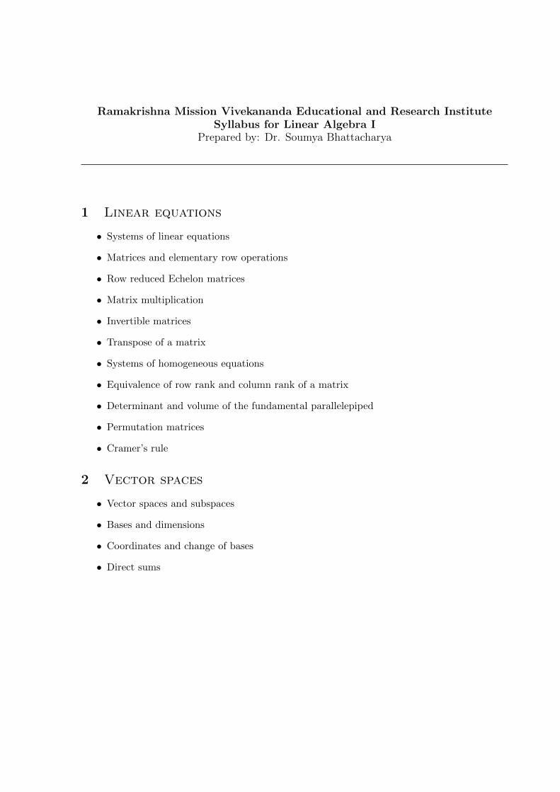
Ramakrishna Mission Vivekananda Educational and Research InstituteSyllabus for Linear Algebra I

Prepared by: Dr. Soumya Bhattacharya

1 Linear equations

• Systems of linear equations

• Matrices and elementary row operations

• Row reduced Echelon matrices

• Matrix multiplication

• Invertible matrices

• Transpose of a matrix

• Systems of homogeneous equations

• Equivalence of row rank and column rank of a matrix

• Determinant and volume of the fundamental parallelepiped

• Permutation matrices

• Cramer’s rule

2 Vector spaces

• Vector spaces and subspaces

• Bases and dimensions

• Coordinates and change of bases

• Direct sums

3 Linear transformations

• The Rank-Nullity theorem

• Matrix of a linear transformation

• Linear operators and isomorphism of vector spaces

• Determinant of a linear operator

• Linear functionals

• Annihilators

• The double dual

4 Eigenvalues and eigenvectors

• Eigenvalues and eigenvectors of matrices

• The characteristic polynomial

• Algebraic and geometric multiplicities of eigenvalues

• Diagonalizability

• Cayley-Hamilton theorem

• Solving linear recurrences

5 Bilinear forms

• Matrix of a bilinear form

• Symmetric and positive definite bilinear forms

• Normed spaces

• Cauchy-Schwarz inequality and triangle inequality

• Angle between two vectors

• Orthogonal complement

• Projection

• Gram-Schmidt orthogonalization

• Hermitian operators

• The Spectral theorem

Page 2

6 Introduction to linear programming

• Bounded and unbounded sets

• Convex functions

• Convex cone

• Interior points and boundary points

• Extreme points or vertices

• Convex hulls and convex polyhedra

• Supporting and separating hyperplanes

• Formulating linear programming problems

• Feasible solutions and optimal solutions

• Graphical method

• The basic principle of Simplex method

• Big-M method

Reference books

1. M. Artin, Algebra, Prentice Hall.

2. K. M. Hoffmann, R. Kunze, Linear Algebra, Prentice Hall.

3. G. Strang, Introduction to Linear Algebra, Wellesley-Cambridge Press.

4. L. I. Gass, Linear Programming, Tata McGraw Hills.

5. G. Hadley, Linear Programming, Narosa Publishing House.

The students by the end of the course will be able to explain:

• How to check whether a given system of linear equations has any solution or not.

• How to find the solutions (if any) of a system of linear equations.

• Why a system of linear equations with more variables than equations always has a solution,whereas a system of such equations with more equations than variables may not have anysolution at all.

• How to find the rank and nullity of a matrix.

• Why each permutation matrix is of full rank.

Page 3

• Why a matrix is invertible if and only if it has nonzero determinant and how to find theinverse of such a matrix.

• Why a matrix with more columns than rows (resp. more rows than columns) does nothave a left (resp. right) inverse.

• How to extend a basis of a subspace of a vector space V to a basis of V .

• How a change of basis affects the coordinates of a given vector.

• Why both the ranks of a matrix A and its transpose AT are the same as that of ATA.

• Why the determinant of the matrix of a linear operator does not depend on the choice ofthe basis of the ambient space.

• Why the sum of the dimension of a subspace W of a vector space V and the dimension ofthe annihilator of W is the dimension of V .

• Why the double dual of a vector space V is canonically isomorphic to V itself.

• Why the fact that a certain conjugate of a given matrix A is diagonal is equivalent to thefact that the space on which A acts by left multiplication is a direct sum of the eigenspacesof A.

• Why every idempotent matrix is diagonalizable.

• Why conjugate matrices have the same eigenvalues with the same algebraic and geometricmultiplicities.

• What Cayley-Hamilton theorem states and why replacing the variable t by the squarematrix A in det(tI −A) does not lead to a proof of this theorem.

• How to solve a linear recurrence whose associated matrix is diagonalizable.

• Why the determinant of an upper or lower triangular matrix is the product of its diagonalentries.

• Why two diagonalizable matrices commute if and only if they are simultaneously diago-nalizable.

• Why for a matrix which represent the dot product with respect to some basis, it is necessaryand sufficient to be symmetric and positive definite.

• Why for a symmetric matrix to be positive definite, it is necessary and sufficient for it tohave strictly positive eigenvalues.

• What is the role of the Cauchy-Schwarz inequality in defining the angle between twovectors.

• Why the elements in a basis a subspaceW of V and the elements in a basis of the orthogonalcomplement of W are linearly independent.

• How to orthogonalize a given basis of an inner product space.

Page 4

• Why each inner product on a real vector space V induces an isomorphism between V andits dual.

• Why any symmetric matrix is diagonalizable and why all its eigenvalues are real.

• Why in a closed and bounded convex region, a convex function attains its maximum atthe boundary.

• Why it suffices to check only the corner points to find a solution to a given linear pro-gramming problem, whose feasible region is a convex polyhedron.

Sample questions

Linear equations

1. Let A be a square matrix. Show that the following conditions are equivalent:

(i) The system of equations AX = 0 has only the trivial solution X = 0.

(ii) A is invertible.

2. Show that a matrix with more columns than rows (resp. more rows than columns) does nothave a left (resp. right) inverse.

3. Explain why a system of linear equations with more variables than equations always has asolution, whereas a system of such equations with more equations than variables may not haveany solution at all.

4. Let An = 0. Let I denote the identity matrix of the same size as that of A. Compute theinverse of A− I.

5. Prove that if A is invertible, then (At)−1 = (A−1)t.

6. Compute the determinant of the following matrix:

2 1

1 2 1 01 2 1

. . .. . .

. . .

0 1 2 1

1 2

n×n

.

Page 5

7. Let n be a positive integer and let

A =

2 −1

−1 2 −1 0−1 2 −1

. . .. . .

. . .

0 −1 2 −1

−1 2

n×n

.

Find the value of the determinant of the matrix A.

8. Show that every permutation matrix is of full rank.


2 −2

−1 5 −2 0−2 5 −2

. . .. . .

. . .

−2 5 −2

0 −2 5 −1

−2 2

n×n

.


3 2

1 3 2 01 3 2

. . .. . .

. . .

0 1 3 2

1 3

n×n

.

11. If possible, find all the solutions of the equation XY − Y X = I in 3× 3 real matrices X,Y .

12. Let A ∈Mn,n(R). Show that

(detA)2 ≤n∏i=1

(n∑k=1

A2k,i

),

where Ak,i denotes the k, i-th entry of A.

Page 6

13. Let

A =

2 −2 −4−1 3 41 −2 −3

∈M3,3(R).

Find the inverse of the matrix(37 ·A372 + 2 · I

).

Vector spaces and linear transformations

14. Let f and g be two nonzero linear functionals on a finite dimensional real vector space Vsuch that their nullspaces (i.e. kernels) coincide. Show that there exists a c ∈ R such thatf = cg.

15. Show that if the product of two n× n matrices is 0, then sum of their ranks is less than orequal to n.

16. The cross product of two vectors in R3 can be generalized for n ≥ 3 to a product of n − 1vectors in Rn as follows: For x(1), . . . , x(n−1) ∈ Rn, define

x(1) × . . .× x(n−1) :=n∑i=1

(−1)i+1(detAi) · ei,

where A ∈Mn−1,n(R) is the matrix, whose rows are x(1), . . . , x(n−1) and Ai is the submatrix ofA obtained by deleting the i-th column of A. Similarly as in the case n = 3, the cross productx(1) × · · · × x(n−1) is given by the formal expansion of

det

e1 e2 · · · en

x(1)1 x

(1)2 · · · x

(1)n

......

...

x(n−1)1 x

(n−1)2 · · · x

(n−1)n

w.r.t. the first row. Show that the following assertions hold for the generalized cross product:

a) x(1)× . . .×x(i−1)×(x+y)×x(i+1)× . . .×x(n−1) = x(1)× . . .×x(i−1)×x×x(i+1)× . . .×x(n−1)+x(1) × . . .× x(i−1) × y × x(i+1) × . . .× x(n−1).

b) x(1)×. . .×x(i−1)×λx×x(i+1)×. . .×x(n−1) = λ(x(1) × . . .× x(i−1) × x× x(i+1) × . . .× x(n−1)

).

c) x(1) × . . .× x(n−1) = 0 ⇔ x(1), . . . , x(n−1) are linearly dependent.

d) 〈x(1) × . . .× x(n−1), y〉 = det

y1 y2 · · · yn

x(1)1 x

(1)2 · · · x

(1)n

......

...

x(n−1)1 x

(n−1)2 · · · x

(n−1)n

.

e) 〈x(1) × . . .× x(n−1), x(i)〉 = 0 for i ∈ {1, . . . , n− 1}.

17. For any matrix A, show that the ranks of A and ATA are the same.

Page 7

18. Let n ≥ 3, A ∈ On and x(1), . . . , x(n−1) ∈ Rn. Define the linear map ϕA : Rn −→ Rn byϕ(v) = Av and let the generalized cross product of n− 1 vectors in Rn be defined as in the lastexercise. Show that:

ϕA(x(1)

)× · · · × ϕA

(x(n−1)

)= detA · ϕA

(x(1) × · · · × x(n−1)

).

19. Let V and W be finite dimensional vector spaces and let iV : V → V and iW : W →W beidentity maps. Let φ : V → W and ψ : W → V be two linear maps. Show that iV − ψ ◦ φ isinvertible if and only if iW − φ ◦ ψ is invertible.

20. If W1 and W2 are two subspaces of a vector space V , then show that

(W1 +W2)0 = W 0

1 ∩W 02 .

21. If W1 and W2 are two subspaces of a vector space V , then show that

(W1 ∩W2)0 = W 0

1 +W 02 .

22. Let V = R3 and let B =

1

03

,

112

,

011

be a basis of V . Compute the dual basis B∗

of V ∗.

23. Let V,W finite dimensional vector spaces over a field K and let ϕ : V →W be a linear map.(1) Show that ϕ∗ : W ∗ → V ∗ is a linear map.(2) Show that ψ : HomK(V,W ) −→ HomK(W ∗, V ∗), ϕ 7→ ϕ∗ is an isomorphism.

24. Let V,W be finiet dimensional vector spaces over a field K and let ϕ : V → W be a linearmap.(1) Show that if ϕ is surjective, then ϕ∗ injective.(2) Show that if ϕ is injective, then ϕ∗ is surjective.

Eigenvalues and eigenvectors

25. Let A be a diagonalizable matrix. Show that A and AT are conjugate.

26. Let v, w ∈ Rn are eigenvectors of a matrix A ∈ Mn,n(R) with corresponding eigenvalues λand µ respectively. Show that if v + w is also an eigenvector of A, then λ = µ.

27. Let V = Rn and A ∈Mn,n(R) be a diagonalizable matrix. Show that:

V = (ker ϕA)⊕ (Im ϕA),

where the map ϕA : V −→ V is defined by ϕA(v) := Av for all v ∈ V .

28. Find a closed formula for the n-th term of the linear recurrence defined as follows: F0 =0, F1 = 1 and

Fn+1 = 3Fn − 2Fn−1.

Page 8

29. Let A ∈ On with detA = −1. Show that −1 is an eigenvalue of A with an odd algebraicmultiplicity.

30. Let n be a positive odd integer and let A ∈ SOn. Show that 1 is an eigenvalue of A.

31. If each row sum of a real square matrix A is 1, show that 1 is an eigenvalue of A.

32. Let A be a 2017× 2017 matrix with all its diagonal entries equal to 2017. If all the rest ofthe entries of A are 1, find the distinct eigenvalues of A.

33. Let λ be an eigenvalue of the n × n matrix A = (aij). Show that there exists a positiveinteger k ≤ n such that

|λ− akk| ≤n∑

j=1, j 6=k|ajk|.

34. Let A be a diagonalizable matrix. Show that A and AT have the same eigenvalues with thesame algebraic and geometric multiplicities.

35. (a) Let A be a 3× 3 matrix with real entries such that A3 = A. Show that A is diagonaliz-able.(b) Let n be a positive integer. Let A be a n × n matrix with real entries such that A2 = A.Show that A is diagonalizable.

36. Let A be a diagonalizable matrix. Show that A and AT have the same eigenvalues with thesame algebraic and geometric multiplicities.

37. Let A be a 3 × 3 matrix with positive determinant. Let PA(t) denote the characteristicpolynomial of A. If PA(−1) > 1, show that A is diagonalizable.

38. Let A be a 3× 3 matrix with real entries. If PA(−1) > 0 > PA(1), where PA(t) denotes thecharacteristic polynomial of A, show that A is diagonalizable.

39. (a) Show that similar matrices (i.e. conjugate matrices) have the same eigenvalues with thesame algebraic and geometric multiplicities.(b) Give examples of two matrices with the same characteristic polynomial but with an eigenvaluewhich does not have the same geometric multiplicity.

40. Let A be a 3× 3 matrix with real entries such that A3 = A. Show that A is diagonalizable.

41. Let n be a positive integer and let A be a n× n matrix with real entries such that A3 = A.Show that A is diagonalizable.

42. For an n× n matrix A and be the characteristic polynomial PA(t) of A, is the following acorrect proof of Cayley-Hamilton theorem?

PA(A) = det(A · In −A) = det(A−A) = 0.

Justify your answer.

Page 9

43. Determine the eigenvalues of the orthogonal matrix

A =1

2·

1 + 1√2−1 1√

2− 1

1− 1√2

1 − 1√2− 1

1√

2 1

.

44. (a) Find a closed formula for the n-th term of the linear recurrence defined as follows:F0 = 0, F1 = 1 and

Fn+1 = 2Fn + Fn−1

by diagonalizing the matrix

(2 11 0

).

(b) Explain why the above method fails to help us in finding a closed formula for the n-th termof the linear recurrence defined as follows: F0 = 0, F1 = 1 and

Fn+1 = 2Fn − Fn−1.

45. Let A be a 5 × 5 real matrix with negative determinant. If PA(±2) > 0 > PA(±1), wherePA(t) denotes the characteristic polynomial of A, show that A is diagonalizable.

46. We say that two matrices A and B are simultaneously diagonalizable if there exists aninvertible matrix P such that both PAP−1 and PBP−1 are diagonal. Show that two diago-nalizable matrices A and B commute with each other if and only if they are simultaneouslydiagonalizable.

47. Find a closed formula for the n-th term of the linear recurrence defined as follows: F0 = 0,F1 = 1 and

Fn+1 = 3Fn − 2Fn−1.

48. Solve the following equation for a 2× 2 matrix X:

X2 =

(5 44 5

).

49. Let

A =

3 −1 11 −1 11 −1 3

and B =

3 1 1−1 −1 −11 1 3

.

Without doing any calculations, explain for which one of the matrices A + B and AB, theeigenvectors form a basis of R3.(b) (3 points) Determine that basis of eigenvectors of R3 for one of the matrices A+B or AB.

50. Construct and example of the scenario where α, β, γ ∈ Rn such that α ⊥ β, γ 6= 0 and A,B are n× n matrices such that A · α = aγ and B · β = bγ, where a is a nonzero eigenvalue of Aand b is a nonzero eigenvalue of B.

Page 10

Bilinear forms

51. How many n× n real matrices are both symmetric and orthogonal? Justify your answer.

52. We call a linear map Rn an isometry if it preserves the dot product on Rn. Show that leftmultiplication by a real square matrix A defines an isometry on Rn if and only if A is orthogonal.

53. How many n×n complex matrices are there which are positive definite, self-adjoint as wellas unitary?

54. For any complex square matrix A, show that the ranks of A and A∗ are equal.

55. Show that if the columns of a square matrix form an orthonormal basis of Cn, then its rowsdo too.

56. Let B ∈Mn,n(R). Show that

ker ϕB := (Im ϕBT)⊥,

where the map ϕB : Rn −→ Rn is defined by ϕB(v) = Bv.

57. Let V = R4 and let f : V −→ V such that f2 = 0. Show that for each triplet v1, v2, v3 ∈Im f , we have

Vol(v1, v2, v3) = 0.

58. Let V = C2 and let s be a symmetric bilinear form on V . Let q : V −→ R be the quadraticform corresponding to s. Suppose, for all z1, z2 ∈ C, we have

q

((z1z2

))= |z1|2 + |z2|2 + i(z1z2 − z1z2).

Compute the determinant of the matrix representing s with respect to the basis B =

{(1i

),

(1 + i

1

)}.

59. Let V be a real vector space with inner product s and let v1, . . . , vn ∈ V r {0} such thats(vi, vj) = 0 for all i, j ∈ {1, . . . , n}. For v ∈ V , we define ‖v‖ =

√s(v, v).

(1) Show that for all v ∈ V , we have

n∑i=1

s(v, vi)2

‖vi‖2≤ ‖v‖2 . (1)

(2) Determine all the cases when the equality holds in (1).

60. Let V be a finite dimensional vector space and let P and Q be projection maps from V toV . Show that the following are equivalent:

(a) P ◦Q = Q ◦ P = 0.

(b) P +Q is a projection.

Page 11

(c) P ◦Q+Q ◦ P = 0.

61. Let V = R3 be the three dimensional euclidean space with the usual dot product and let

U be the subspace of V which is spanned by

1−10

and

101

. Determine the matrix of the

orthogonal projection PU with respect to the standard basis of V .

62. Do the following exercise without using the Spectral Theorem:

(1) Let A =

(a bb d

)∈M2,2(R). Show that A is diagonalizable.

(2) Let B ∈M3,3(R) be a symmetric matrix. Show that B is diagonalizable.

63. Let V be a finite dimensional real vector space. For v, w ∈ V \ {0}, we define the angle](v, w) between the vectors v und w as the uniquely determined number ϑ ∈ [0, π], for which

s(v, w) = cosϑ ‖v‖‖w‖.

We call ϕ ∈ End(V ) conformal if ϕ is injective and if

](v, w) = ](ϕ(v), ϕ(w)) for all v, w ∈ V \ {0}.

Show that a linear map ϕ is conformal if and only if there exists an isometry ψ ∈ End(V ) anda λ ∈ R \ {0} such that ϕ = λ · ψ.

64. Find all the unitary matrices A such that s(v, w) := 〈v,Aw〉 defines an inner product onCn, where 〈 , 〉 denotes the canonical inner product on Cn.

65. Let V be a finite dimensional vector space over R. Show that each bilinear form on V canbe uniquely written as the sum of a symmetric and a skew-symmetric bilinear form.

66. Let s be a symmetric bilinear form on a vector space V . If there are vectors v, w ∈ V , suchthat s(v, w) 6= 0, show that there is a vector v ∈ V , such that s(v, v) 6= 0.

67. Let V be the vector space of the complex-valued continuous functions on the unit circle inC. a) Show that

〈f, g〉 :=

∫ 2π

0f(eiθ)g(eiθ)dθ

defines an inner product on V .b) Define the subspace W ⊆ V by W := {f(eiθ) : f(x) ∈ C[x] and deg(f) ≤ n}. Find anorthonormal basis of W w.r.t. the above inner product.

Page 12

68. Let A be the following 3× 3 matrix:1 1 11 −1 −11 −1 1

.

(a) Without any computation, explain why there must exist a basis of R3 consisting only of theeigenvectors of A.(b) Find such a basis of R3.(c) Determine whether or not the bilinear form s : R3 → R given by s(u, v) := uTAv defines aninner product on R3.

69. (a) Let V be a finite dimensional vector space over R and let f and g be two linear functionalson V such that ker f = ker g. Show that there exists an r ∈ R such that g = rf .(b) Let ϕ1, ϕ2, . . . , ϕ5 be linear functionals on a vector space V such that there does not existany vector v ∈ V for which ϕ1(v) = ϕ2(v) = · · · = ϕ5(v). Show that dimV ≤ 5.

70. Let w =

123

and let the linear map f : R3 → R be defined by

f(v) = vTw

for all v ∈ R3.a) Find an orthonormal basis of Ker f w.r.t. dot product.b) Extend this orthonormal basis of Ker f to an orthonormal basis of R3.

71. Let P2(R) denote the set of polynomials of degree ≤ 2 with real coefficients. Define thelinear map φ : P2(R) → R by φ(f) = f(1). Determine (Ker φ)⊥ with respect to the followinginner product:

s(f, g) =

∫ 1

−1f(t)g(t)dt.

72. Let P3(R) denote the set of polynomials of degree ≤ 3 with real coefficients. On P3(R), wedefine the symmetric bilinear form s by

s(f, g) =

∫ 1

−1f(t)g(t)dt.

a) Determine the matrix representtation of s w.r.t. the basis {1, t, t2, t3}.b) Show that s is positive definit.c) Determine an orthonormal basis of P3(R).

73. Show that the eigenvectors associated with distinct eigenvalues of a self-adjoint matrix areorthogonal.

Page 13

74. Let A ∈ Mn,n(R) have eigenvalues λ1, λ2, . . . , λn ∈ R which are not necessarily distinct.Suppose v1, v2, . . . , vn ∈ Rn are eigenvectors of A associated with the eigenvalues λ1, λ2, . . . , λnrespectively, such that vi ⊥ vj if i 6= j. Show that A is symmetric.

75. Let A ∈ Mn,n(R) a skew symmetric matrix. Let v und w be two eigenvectors of A corre-sponding respectively to the distinct eigenvalues λ1 and λ2. Show that v and w are orthogonalto each other (w.r.t. the dot product).

76. Let A ∈Mn,n(C) be a self-adjoint matrix. Show that the eigenvalues of A are real.

77. How many orthonormal bases (w.r.t. the dot product) are there in Rn , so that all theentries of the basis vectors are integers?

78. Let V = Cn, let A ∈Mn,n(C) a self-adjoint Matrix and let the linear operator φA : V −→ Vbe defined by φA(v) = Av. Let W be a subspace of V , so that φA(W ) ⊆ W (i.e. φA(w) ∈ Wfor all w ∈W ). Show that

φA(W⊥) ∩W = {0}.

79. Let V = R2 and let s a symmetric bilinear form on V . let q : V −→ R be the quadraticform corresponding to s given by

q

((xy

))= x2 + 5xy + y2.

Determine the matrix of s w.r.t. the basis B =

{(21

),

(−12

)}of R2.

80. Let V be a finite dimensional vector space over R with an inner product 〈 , 〉 and letf : V → R be a linear map. Show that there is an uniquely determined vector vf such that forall v ∈ V , we have

f(v) = 〈v, vf 〉.

81. Given

A =

3 −1 0−1 0 10 1 −1

∈M3,3(R),

find a matrix g ∈ GL3(R), such that gTAg is of the formIk −IlO

.

Page 14

82. Draw the curve C :=

{(xy

)∈ R2

∣∣∣∣ 3x2 + 4xy + 3y2 = 5

}.

83. Let X ∈ Mn,n(C) be a self-adjoint matrix and suppose m be a positive integer such thatXm = I. Show that X3 − 2X2 −X + 2I = 0.

84. Let n ∈ Z≥2. Show that s(A,B) := tr(A · BT) defines an inner product on V = Mn,n(R).Let ϕ ∈ End(V ) be defined by

ϕ(A) = AT.

(1) Show that ϕ is hermitian.(2) Show that ϕ is an isometry.(3) Find the eigenvalues of ϕ.(4) Find an orthonormal basis B of V , made up of the eigenvectors ef ϕ.(5) Find the algebraic multiplicities ef the eigenvalues of ϕ.

85. Let for x ∈ R, the matrix Ax defined by

Ax :=1

1 + x+ x2

−x x+ x2 1 + x1 + x −x x+ x2

x+ x2 1 + x −x

.

(1) Show that for all x ∈ R, we have Ax ∈ SO3.(2) Conclude from (1) that for all real x 6= ±1, there exists a gx ∈ O3 and an αx ∈ (0, π)∪(π, 2π)such that

gxAxg−1x =

1 0 00 cosαx − sinαx0 sinαx cosαx

.

(3) Determine the complex eigenvalues of Ax for x = 1 +√

2 +√

3 + 1+√3√

2.

86. (1) Find a matrix g ∈ O2 which diagonalizes the matrix A =

(13 1212 13

).

(2) Find a matrix X ∈ M2,2(R), which defines a scalar product through s(v, w) = 〈v,Xw〉 onR2 and which satisfies the following equation:

X2 −A = 0.

87. Let A ∈Mn,n(R) be a symmetric matrix and let B ∈Mn,n(R) be a skew-symmetric matrix.

Let M = A+ iB and let v :=

λ1...λn

, where λ1, . . . , λn are the eigenvalues of M . Show that

‖v‖ =

√√√√ n∑j,k=1

|Mjk|2,

w.r.t. the canonical norm on Cn.

Page 15

88. Let φ : Cn → Cn be a nilpotent, hermitian endomorphism. Show that: φ = 0.

89. Let A,B ∈Mn,n(C) be two self-adjoint matrices. Show that the following are equivalent:(1) There is an unitary matrix g such that both gAg−1 and gBg−1 are diagonal matrices.(2) The matrix AB is self-adjoint.(3) AB = BA.

90. (1) Let A,B ∈Mn,n(C) be nilpotent matrices such that AB = BA holds. Show that A+Bis nilpotent.(2) Let A,B ∈ Mn,n(C) and r, s ∈ Z>0 such that Ar = I, Bs = 0 and AB = BA. Show thatA−B is invertible.

91. Let

A =

1 −2 20 −2 1−2 1 −2

∈M3,3(R).

(1) Find a decomposition A = D+N , where D is a diagonal matrix an N is a nilpotente Matrix.(2) Berechnen Sie A2012.

92. Let A ∈Mn,n(R) be a nilpotent matrix and let V = Mn,n(R). Let ϕ ∈ End(V ) defined by

ϕ(B) = AB −BA for B ∈ V .

Show that ϕ is nilpotent on V .

93. Let V = Rn with s = 〈·, ·〉 and let B = {v1, . . . , vn} an orthonormal basis of V . LetUi = (span{vi})⊥ for i ∈ {1, . . . , n}. Show that

SUi ◦ SUj = SUj ◦ SUi

for i, j ∈ {1, . . . , n}, where SUi and SUj are the reflections in Ui and Uj .

94. Let V be a finite dimensional vectore space and let P ∈ End(V ) be a projektion. LetId ∈ End(V ) the identity map of V (i.e. Id(v) = v for all v ∈ V ). Show that(1) Id−P is a projektion.(2) Id−2P is bijective.(3) E0 ⊕ E1 = V , where E0 and E1 are respectively the eigenspaces of P corresponding to theeigenvalues 0 and 1.

95. Let A ∈Mn,n(C) and let B = A−A∗. Show that B is diagonalizable and the real parts ofall the eigenvalues of B are zero.

Page 16

96. Let A ∈ SO2. Show that there is a skew symmetric matrix X ∈M2,2(R), such that

exp(X) = A.

97. Let V = R5 and let ` ∈ V ∗ be given by `(v) = v1 + 2v2 + 3v3 + 4v4 + 5v5 fur v =

v1...v5

∈ V .

(1) Find an orthonormal basis of ker ` w.r.t. the dot product.(2) Extend this basis of ker ` to an orthonormal basis of V .

98. Let V = R4, let

A =1

2

2 1 2 −31 2 −3 22 −3 2 1−3 2 1 2

∈M4,4(R)

and let s be the symmetric bilinear form whose associated matrix is A.(1) Determine a basis A of V , such that MA(s) is a diagonal matrix.(2) Determine a basis B of V , such that

MB(s) =

Ik −IlO

.

99. Let V = R3 with s = 〈·, ·〉 (the dot product), let U = span

2

10

,

10−1

be a subspace

of V and let SU be the reflection in in U .(1) Determine a matrix representation of SU , w.r.t. the canonical basis A of V .(2) Show that M(SU )A ∈ O3 and decide whether M(SU )A ∈ SO3 oder M(SU )A 6∈ SO3 or not.

Introduction to linear programming

100. Maximize f(x, y, z) := 6x+3y+10z using Simplex method under the following constraints:

4x+ y + z ≤ 5,

2x+ y + 4z ≤ 5,

x+ 5y + z ≤ 6,

where x, y and z are non-negative rational numbers.

101. Minimize f(x, y, z) := x+ 2y + 9z using big-M method under the following constraints:

2x+ y + 4z ≥ 5,

2x+ 3y + z ≥ 4,


Page 17

102. (a) A convex linear combination of v1, v2, . . . , vn ∈ Rm is a a linear combination of theform t1v1 + · · · + tnvn, where t1 + · · · + tn = 1.For example, the points on the straight lineconnecting v1 and v2 is given by tv1 + (1− t)v2, where t lies in the interval [0, 1] ⊂ R. Show thatany arbitrary point in a triangle in Rm with vertices v1, v2 and v3 is given by a convex linearcombination of its vertices.(b) Show that any arbitrary point in a tetrahedron in Rm with vertices v1, v2, v3 and v4 is givenby a convex linear combination of its vertices.

103. Let f : R2 → R be defined by f(x, y) := 2x+ 3y. Find the maximum value attained by fin the region where 2y − x ≤ 10, 3x+ 2y ≤ 9 and 2x+ 5y ≥ 8.

104. Maximize f(x, y, z) := 2x+5y+3z using Simplex method under the following constraints:

14x+ 8y + 5z ≤ 15,

12x+ 7y + 8z ≤ 14,

3x+ 17y + 9z ≤ 16,


105. Minimize f(x, y, z) := x+ 9y + 9z using big-M method under the following constraints:

6x+ y + 5z ≥ 11,

4x+ 7y + 2z ≥ 9,


106. (a) Recall that any arbitrary point in a convex polyhedron is given by a convex linearcombination of its vertices. Using this, show that the minimum and the maximum valuesattained by a linear functional f : Rn → R in a convex polyhedron P ⊂ Rn is the same as theminimum and the maximum values attained by f at the set of the vertices of P.(b) Let f : R2 → R be defined by f(x, y) := 5x− 3y. Find the maximum value attained by f inthe region where 4y − 3x ≤ 10, 7x+ 2y ≤ 9 and 2x+ 5y ≥ 8.

107. Maximize f(x, y, z) := 3x+ y+ 3z using Simplex method under the following constraints:

2x+ y + z ≤ 2,

x+ 2y + 3z ≤ 5,

2x+ 2y + z ≤ 6,


108. Maximize f(x, y, z) := 3x+ y + 4z using big-M method under the following constraints:

x+ 3y + 4z ≤ 20,

2x+ y + z ≥ 8,

3x+ 2y + 3z = 18,


Page 18

Department of Computer Sc. RKMVERI Belur CS 244 Syllabus

CS 244 : Introduction to Optimization TechniquesCourse Overview: The process of making optimal judgement according to various criteria is known as the

science of decision making. A mathematical programming problem, also known as an optimization problem,is a special class of problem where we are concerned with the optimal use of limited resources to meet somedesired objective(s). Mathematical models (simulation based and/or analytical based) are used in provid-ing guidelines for making effective decisions under constraints. This course covers three major analyticaltopics in mathematical programming [linear, nonlinear and integer programming]. On each topic, the the-ory and modeling aspects are discussed first, and subsequently solution techniques or algorithms are covered.

Prerequisite(s): Linear AlgebraCredit Hours: 4Course Objectives: Optimization techniques are used in various fields like machine learning, graph the-ory, VLSI design and complex networks. In all these applications/fields, mathematical programming theorysupplies the notion of optimal solution via the optimality conditions, and mathematical programming algo-rithms provide tools for training and/or solving large scale models. Students will have knowledge of theoryand applications of several classes of math programs.

Text(s): The course material will be drawn from multiple book chapters, journal articles, reviewed tutorialsetc. However, the following two books are recommended texts for this course.

• Linear programming and Network Flows, Wiley-Blackwell; 4th Edition, 2010M. S. Bazaraa, John J. Jarvis and Hanif D. Sheral, ISBN-13: 978-0470462720

• Nonlinear Programming: Theory and Algorithms, Wiley-Blackwell; 3rd Edition (2006)M. S. Bazaraa, Hanif D. Sherali, C. M. Shetty, ISBN-13: 978-0471486008

Course Policies:

• Grades

Grades in the C range represent performance that meets expectations; Grades in the B rangerepresent performance that is substantially better than the expectations; Grades in the Arange represent work that is excellent.

• Assignments

1. Students are expected to work independently. Discussion amongst students is encouraged butoffering and accepting solutions from others is an act of dishonesty and students can be penalizedaccording to the Academic Honesty Policy.

2. No late assignments will be accepted under any circumstances.

• Attendance and Absence

Students are not supposed to miss class without prior notice/permission. Students are responsiblefor all missed work, regardless of the reason for absence. It is also the absentee’s responsibility toget all missing notes or materials.

Grade Distribution:Assignments 40%Midterm Exam 20%Final Exam 40%

Grading Policy: Approximate grade assignments:>= 90.0 % A+75.0 – 89.9 % A60.0 – 74.9 % B50.0 – 59.9 % Cabout 35.0 – 49.9 % D<= 34.9% F

Page 1

Department of Computer Sc. RKMVERI Belur CS 244 Syllabus

Table 1: Topics Covered

Mathematical Preliminaries

• Theory of Sets and Functions,• Vctor spaces,• Matrices and Determinants,• Convex sets and convex cones,• Convex and concave functions,• Generalized concavity

Linear Programming

• The (Conventional) Linear Programming Model• The Simplex Method: Tableau And Computation• Special Simplex Method And Implementations• Duality And Sensitivity Analysis

Integer Programming

• Formulating Integer Programing Problems• Solving Integer Programs (Branch-and-Bound Enumeration, Implicit Enumeration,

Cutting Plane Methods )

Nonlinear Programming: Theory

• Constrained Optimization Problem (equality and inequality constraints)• Necessary and Suffiecent conditions• Constraint Qualification• Lanrangian Duality and Saddle Point Optimality Criteria

Nonlinear Programming: Algorithms

• The concept of Algorithm• Algorithms for Uconstrained Optimization• Constraint Qualification• Algorithms for Constrained Optimization (Penalty Function, Barrier Function, Feasi-

ble Direction)

Special Topics (if time permits)

• Semi-definite and Semi-infinte Programs• Quadratic Programming• Linear Fractional programming• Separable Programming

Page 2

DA311

Time Series


Dr. Sudipta Das

[email protected]

Office: IH404, Prajnabhavan, RKMVERI, BelurOffice Hours: 11 pm—12 noon, 3 pm—4 pm(+91) 99039 73750

Course Description: DA311 is going to provide a broad introduction to the most fundamental method-ologies and techniques used in time series analysis.

Prerequisite(s): (1) Probability & Stochastic Process and (2) Linear Algebra.Note(s): Syllabus changes yearly and may be modified during the term itself, depending on the circum-stances. However, students will be evaluated only on the basis of topics covered in the course.Course url:Credit Hours: 4

Text(s):

Introduction to time series analysis;PJ Brockwell and RA Davis

Time Series Analysis and Its Applications;Robert H. Shumway and David S. Stoffer

Introduction to Statistical time series;WA Fuller

Time Series Analysis;Wilfredo Palma

Course Objectives:

Knowledge acquired: Students will get to know(1) Different time series models MA, AR, ARMA, ARIMA(2) Autocorrelation and Partial Autocorrelation functions,(3) Method of time series modelling, in presence of seasonality, and,(4) Different non-linear time series models such as ARCH and GARCH.

Skills gained: The students will be able to(1) explore trend and seasonality in time series data by exploratory data analysis,(2) implement stationary as well as non-stationary models through parameter estimation,(3) compute forecast for time series data.

1

Grade Distribution:Assignments 20%Quizzes 10%Midterm Exam 20%Final Exam 50%

Grading Policy: There will be relative grading such that the cutoff for A grade will not be less than75% and cutoff for F grade will not be more than 34.9%. Grade distribution will follow normal bell curve(usually, A: ≥ µ + 3σ/2, B: µ + σ/2 . . . µ + 3σ/2 C: µ − σ/2 . . . µ + σ/2, D: µ − 3σ/2 . . . µ − σ/2, and F:< µ− 3σ/2)Approximate grade assignments:

>= 90.0 A+75.0 – 89.9 A60.0 – 74.9 B50.0 – 59.9 Cabout 35.0 – 49.9 D<= 34.9 F

Course Policies:

• General

1. Computing devices are not to be used during any exams unless instructed to do so.

2. Quizzes and exams are closed books and closed notes.

3. Quizzes are unannounced but they are frequently held after a topic has been covered.

4. No makeup quizzes or exams will be given.

• Grades

Grades in the C range represent performance that meets expectations; Grades in the B rangerepresent performance that is substantially better than the expectations; Grades in the Arange represent work that is excellent.

• Labs and Assignments

1. Students are expected to work independently. Offering and accepting solutions from others isan act of dishonesty and students can be penalized according to the Academic Honesty Policy.Discussion amongst students is encouraged, but when in doubt, direct your questions to theprofessor, tutor, or lab assistant. Many students find it helpful to consult their peers while doingassignments. This practice is legitimate and to be expected. However, it is not acceptable practiceto pool thoughts and produce common answers. To avoid this situation, it is suggested thatstudents not write anything down during such talks, but keep mental notes for later developmentof their own.

2. No late assignments will be accepted under any circumstances.

• Attendance and Absences

1. Attendance is expected and will be taken each class. Students are not supposed to miss classwithout prior notice/permission. Any absences may result in point and/or grade deductions.

2. Students are responsible for all missed work, regardless of the reason for absence. It is also theabsentee’s responsibility to get all missing notes or materials.

2


Week Content

Week 1• The Nature of Time Series Data• Financial, Economic, Climatic, Biomedical, Sociological Data.• Reading assignment: Chapter 1, BD

Week 2

• Time Series Statistical Models• Components of time series: Trend, Seasonality and randomness• Whiteness Testing• Quiz 1

Week 3

• Stationary time series• Linear process• Strong and weak stationarity• Causality, invertibility and minimality• Reading assignment: Chapter 2, BD

Week 4

• Auto Regressive model• Moving Average model• Auto Regressive model• Moving Average models

Week 5

• Auto-covariance Function• Auto-correlation Function• Partial Auto-correlation Function• Reading assignment: Chapter 3, BD

Week 6

• Estimating Sample mean,• Estimating Auto-correlation function• Estimating Partial autocorrelation functions• Quiz 2

Week 7

• YuleWalker estimation• Burgs algorithm• Maximum Likelihood Estimation• Reading assignment: Chapter 5, BD

Week 8• Order Selection• The AIC, BIC and AICC criterion• Review for Midterm Exam

3

Week Content

Week 9• Forecasting• Minimum MSE Forecast• Forecast Error

Week 10• Forecasting Stationary Time Series• The DurbinLevinson Algorithm• The Innovations Algorithm

Week 11• Non-stationarity time series• Unit root tests• Reading assignment: Chapter 6, BD

Week 12• ARIMA Processes• Forecasting ARIMA Models• Quiz 3

Week 13• Modelling seasonal time series• Seasonal ARIMA Models• Forecasting SARIMA Processes

Week 14• Nonlinear Time Series• Testing for Linearity• Heteroskedastic Data

Week 15

• Auto-regressive conditional heteroskedastic model• Generalized auto-regressive conditional heteroskedastic model• Reading assignment: Chapter 5, SS• Review for Final Exam

4

DA101

Computing for Data Science

Time: TBA

Place: MB212 / Vijnana Computing Lab

Instructor: Dhyanagamyananda

[email protected], [email protected]

url: http://cs.rkmvu.ac.in/~swat/Office: MB205, Medhabhavan, RKMVERI, BelurOffice Hours: 10 pm—12 noon, 3 pm—5 pm(+91) 033-2654 9999

Course Description: DA101 is an introductory course in Data Science giving anoverview of programming, and computing techniques. This course is specially designed forstudents of Mathematics, Physics, and Statistics.

Prerequisite(s): (1) Basic logic and mathematics.Note(s): Syllabus changes yearly and may be modified during the term itself, depending onthe circumstances. However, students will be evaluated only on the basis of topics coveredin the course.Moodle url: http://moodle.rkmvu.ac.in/course/view.php?id=58Credit Hours: 4

Text(s):

Algorithms in Data Science, First editionBrian Steele, John Chandler, & Swarna Reddy

How to proram in Python

Louden & Louden

How to proram in Java

Louden & Louden

Relevant Internet resources

Course Objectives:

Knowledge acquired: .

1

(1) Turing machine model of computing.(2) Computer programming in python and java.(3) Algorithm design and analysis(4) Simulation.

Skills gained: The students will be able to1. distinguish between computing and non-computing tasks.2. read and understand a program written in Python, and Java.3. represent basic data as data structures suited to computing.4. break down a computing problem into individual steps and code them in python orjava.5. measure the performance and efficiency of an algorithm in terms of time and spacecomplexity.6. understand graph theoritical concepts applied to algorithm.7. interact with relational database using sql.8. use simulation techniques in solving computational problems.

Grade Distribution:Assignments 20%Quizzes 10%Midterm Exam 20%Final Exam 40%

Grading Policy: There will be relative grading such that the cutoff for A grade will notbe less than 75% and cutoff for F grade will not be more than 34.9%. Grade distribution willfollow normal bell curve (usually, A: ≥ µ+3σ/2, B: µ+σ/2 . . . µ+3σ/2 C: µ−σ/2 . . . µ+σ/2,D: µ− 3σ/2 . . . µ− σ/2, and F: < µ− 3σ/2)Approximate grade assignments:

>= 90.0 A+75.0 – 89.9 A60.0 – 74.9 B50.0 – 59.9 Cabout 35.0 – 49.9 D<= 34.9 F

Course Policies:

• General course policies, Grades, Labs and assignments, Attendance andAbsences These clauses are common to all courses. And it can be found in theprogram schedule.

Course Outline (tentative) and Syllabus:The weekly coverage might change as it depends on the progress of the class. However, youmust keep up with the reading assignments. Each week assumes 4 hour lectures. Quizzeswill be unannounced.

2

Week Content

Week 1• Definition of computing, Binary representation of numbers intergers,floating point, text.

• Reading assignment:

Week 2

• Unconventional / application specific file formats, like media. Bitmaprepresentation for monochromatic image and generalizing the represen-tation for RGB. File metadata, Speed of CPU, Memory, Secondary stor-age, DMA. Hardisk organization into Cylinder, Track, and Sectors forstoring data.

• Reading assignment: XBitmap from Wiki.• Programming assignment 1:• Quiz 1

Week 3 • Using and understanding the basics of Linux.• Lab activity.

Week 4

• Learning programming using Python. arrays([], [][]), conditional struc-tures (if), and iterative structures (while, for), defining functions, usinglibrary functions.

• Programming assignment:

Week 5

• Dictionary data structure in python, File access in python, Sorting andSearching algorithms, appreciating complexity of algorithms. Program-ming using numerical methods.

• Programming assignment:• Quiz 2

Week 6

• Basics of Turing machine as a model of computing, analysing the per-formance of a program, time complexity, space complexity, differencebetween efficiency and performance, Analyse the first sorting algorithm.

• Home assignment:

Week 7

• Basic notations of complexity like Big Oh, omega etc, and their mathe-matical definitions, given a programme to compute the complexity mea-sures.

• Reading assignment: Chapter 2.4, BJS• Home assignment:• Quiz 3

Week 8 • Discussion on the reading assignment, and implementing in the lab.• Review for Midterm Exam

3

Week Content

Week 9,10,11

• Programming in SQL (Structured query language) to query relationaldatabases.

• Home assignment 4• Quiz at the end of three weeks.

Week 12

• Representation of graphs, basic algorithms like minimum spanning tree,matching etc.

• Home assignment 7• Quiz 5

Week 13• Monte-Carlo simulation• Reading assignment:• Home assignment 8

Week 14,15,16 • Object oriented programming using Java

4

DA310Multivariate Statistics

Instructor: Sudipta Das

Course Description: This course DA310 deals with a broad introduction to the most fundamentalmethodologies and techniques used in time series analysis

Prerequisite(s): Basic Statistics, Probability and Stochastic ProcessesNote(s): Syllabus changes yearly and may be modified during the term itself, depending on the circum-stances. However, students will be evaluated only on the basis of topics covered in the course.Credit: 2 (four), approximately 32 credit hours

Text(s):

1. Applied multivariate statistical analysis: Richard A. Johnson and Dean W. Wichern, Prentice Hall2002.

Evaluation: Theory 60% + Practical/lab 40%

Course Objectives:

Knowledge gained : At the finish of the course the student will know

• Different matrix operations and SVD

• Multivariate normal distribution and its properties

• Multivariate hypothesis testing

• Multivariate analysis of variance and covariance

• Regression analysis

• principal component analysis

• Discriminant analysis

• Factor analysis

Skills acquired : The student will be able to

• Carry out exploratory multivariate data analysis in R and Excel

• To plot multivariate data and compute descriptive statistics

• Test a data for multivariate normality by graphically and computationally in R

• Perform statistical inference on multivariate means including hypothesis testing, confidence ellip-soid calculation and different types of confidence intervals estimation

• Build multivariate regression model in R

• Extract the features of the data by principal component analysis in R

• Express the data as functions of a number of important causes by the method of factor analysisin R

• To assign objects (or data points) to one group among a number of groups by the method ofdiscriminant analysis in R

Competence developed : The course covers theoretical, computational, and interpretive issues of multi-variate data analysis using R and Excel. Overall, given real data from varied disciplines, students willbe able to apply their mathematical knowledge, methodologies and computational tools to characterizeand analyse it. As a result, important features of the data can be extracted as well some statisticalconclusion can be made.

1

Course Outline (tentative) and Syllabus:

1. Representation of multivariate data, bivariate and multivariate distributions, multinomial distribution,multivariate normal distribution, sample mean and sample dispersion matrix, concepts of locationdepth in multivariate data.(20hrs)

2. Principal component analysis (10hrs)

3. Classification (10hrs)

4. Factor Analysis (10hrs)

5. Clustering (10hrs)

2

DA320 Operations Research

Instructor: Sudeep Mallick

Course Description: CS3210 deals with the topics in problem formulation, modelling and basic so-lution techniques in operations research. It is deemed as a first course in this area. It is intended thatthe course will enable students to take up advanced study in operations research and analytics based onoperations research.

Prerequisite(s): Basic course in Linear Algebra.Credit Hours: 4

Text(s):

1. Operations Research, seventh revised edition (2014), P K Gupta and D S Hira, ISBN: 81-219-0218-9

2. Introduction to Operations Research, eighth edition, Frederick S. Hillier & Gerald J. Lieberman, ISBN:0-07-252744-7

3. Operations Research: An Introduction, ninth edition, Hamdy A. Taha, ISBN: 978-93-325-1822-3

4. AMPL: A Modeling Language for Mathematical Programming, second Edition, www.ampl.com

Course Objectives:Knowledge gained: At the finish of the course the student will know

1) Problem formulation in operations research for problems in various application domains such asoperations management, marketing, production, finance and others.

2) Modelling techniques such as linear programming and translation of any given problem descriptionto a linear programming mathematical model.

3) Solution techniques such as simplex method and its variations and special cases.

4) Effect to change of parameters on a model using basic algebraic sensitivity analysis techniques.

5) Use of software tools to solve simple models

Skills acquired: The students will be able to

1) develop a mathematical model, clearly state model building assumptions starting from a problemdescription.

2) apply the appropriate operations research technique to formulate optimization models.

3) implement and evaluate alternative models of optimization problems using CPLEX software inAMPL modelling language as well as MS-EXCEL.

Competence developed: The student develop the

1. Ability to translate a given problem description into a mathematical model for optimization.

2. Ability to identify and elicit information about the essential parameters of any given optimizationproblem.

3. Ability to identify and use appropriate optimization modelling tools (software) for a given problemsize and description..

Evaluation: Midterm Lab Exam 20% Term Project 40% Endterm Theory Exam 40%


1

www.ampl.com

Week 1• Problem formulation for linear programming problems I

• Reading assignment: Chapter 1, HT

Week 2• Problem formulation for linear programming problems II


Week 3• Problem formulation for linear programming problems III


Week 4• Problem formulation for linear programming problems IV

• Reading assignment: Chapter 1-3, HL

Week 5• Problem formulation for linear programming problems V

• Reading assignment: Chapter 1-3, HL

Week 6

• Solving linear programming problem graphical approach

• RReading assignment: Chapter 3, HT

• Internal test 1

Week 7• Solving linear programming problem algebraic approach

• Reading assignment: Chapter 3, HT / Chapter 4, HL

Week 8• Solving linear programming problem simplex method


Week 9• Solving linear programming problem simplex method variations Big M method and

Artificial variables


Week 10• Solving linear programming problem simplex method special cases degeneracy, alter-

native optima, unbounded solution and infeasible solution


Week 11 • Lab Session: Solving LP problems using AMPL / CPLEX I

Week 12 • Lab Session: Solving LP problems using AMPL / CPLEX - II

• Internal test 2

Week 13• Sensitivity analysis graphical approach


Week 14• Sensitivity analysis algebraic approach


Week 15 • Lab Session: Sensitivity analysis of LP problems using AMPL / CPLEX

• Course review

2

DA240 Introduction to Econometrics

Instructor:

Course Description: This course is going to provide a broad introduction to the most fundamentalmethodologies and techniques used in Econometrics. Students will learn the details of regression analysisand its applications in real life scenario.

Prerequisite(s): NoneCredit: 2 (four), approximately 32 credit hours

Text(s):

1. Introduction to Econometrics by G. S. MADDALA.

Knowledge: The students get to know

• Assumptions of Linear Regression and why are they required.

• The “BLUE” properties of Least Square Estimators.

• Relation between R2 and r2, where r is correlation coefficient between x and y.

• Pairwise correlation tells nothing about multicolinearity except very high correlation near to 1. Evenwith less correlation coefficient value (like 0.2) multicolinearity may occur.

• Test of Multicolinearity. VIF test and its threshold value.

• Dropping a variable from model due to multicolinearity is not a right one.

• Distribution of β (the LS estimator) applying Law of Large Number.

• Detection of heteroscedasticity using different statistical hypothesis testing like Gold-Fields Quandttest, Gleizer test.

• Impact of heteroscedasiticity on β.

• Generalized Least Square Estimation of β.

• Linear Regression when x is stochastic.

• Definition of Exogeneity and Endogeneity.

• Problem of Endogeneity.

• Hypothesis testing (Housman test) to detect Endogeneity

• Handling of Endogeneity by IV estimator(Instrumental Variable).

Evaluation: Theory 60% + Practical/lab 40%


1. Brief discussion about regression analysis.

2. Least Square Estimators

3. Multicolinearity

4. Heteroscedasticity

5. Generalized Least Square Estimation.

6. Exogeneity and Endogeneity.

7. IV estimator(Instrumental Variable)

1

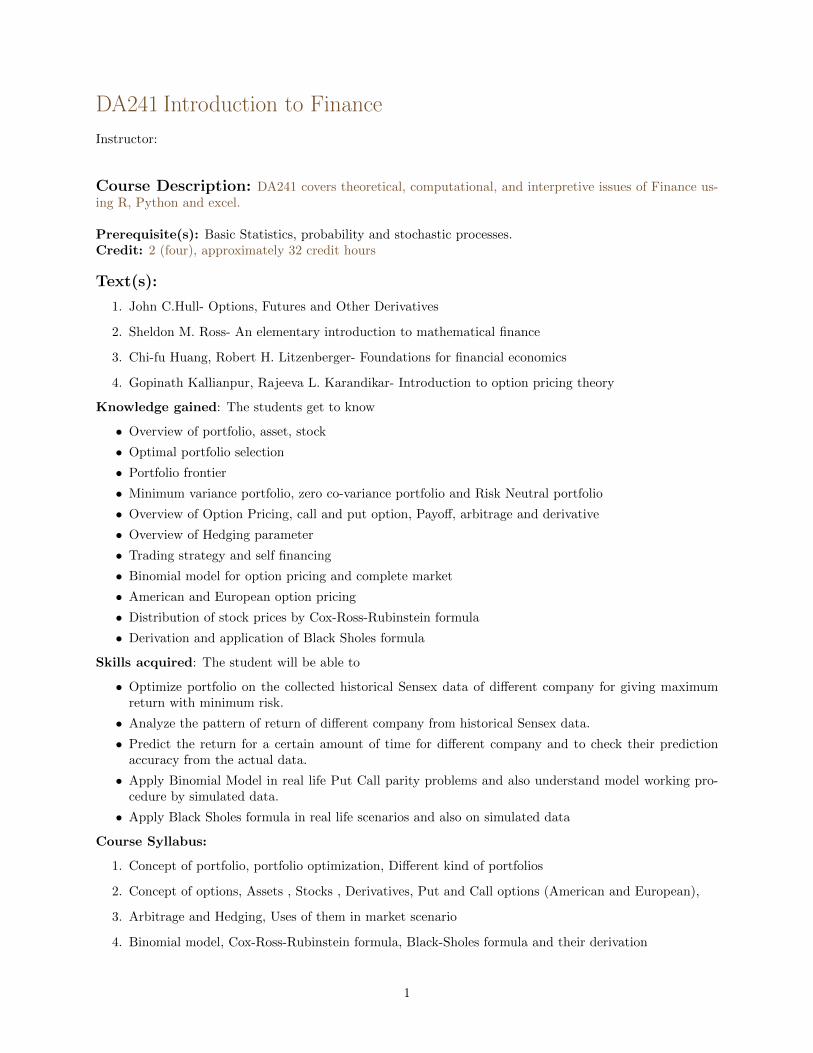
DA241 Introduction to Finance

Instructor:

Course Description: DA241 covers theoretical, computational, and interpretive issues of Finance us-ing R, Python and excel.

Prerequisite(s): Basic Statistics, probability and stochastic processes.Credit: 2 (four), approximately 32 credit hours

Text(s):

1. John C.Hull- Options, Futures and Other Derivatives

2. Sheldon M. Ross- An elementary introduction to mathematical finance

3. Chi-fu Huang, Robert H. Litzenberger- Foundations for financial economics

4. Gopinath Kallianpur, Rajeeva L. Karandikar- Introduction to option pricing theory

Knowledge gained: The students get to know

• Overview of portfolio, asset, stock

• Optimal portfolio selection

• Portfolio frontier

• Minimum variance portfolio, zero co-variance portfolio and Risk Neutral portfolio

• Overview of Option Pricing, call and put option, Payoff, arbitrage and derivative

• Overview of Hedging parameter

• Trading strategy and self financing

• Binomial model for option pricing and complete market

• American and European option pricing

• Distribution of stock prices by Cox-Ross-Rubinstein formula

• Derivation and application of Black Sholes formula

Skills acquired: The student will be able to

• Optimize portfolio on the collected historical Sensex data of different company for giving maximumreturn with minimum risk.

• Analyze the pattern of return of different company from historical Sensex data.

• Predict the return for a certain amount of time for different company and to check their predictionaccuracy from the actual data.

• Apply Binomial Model in real life Put Call parity problems and also understand model working pro-cedure by simulated data.

• Apply Black Sholes formula in real life scenarios and also on simulated data

Course Syllabus:

1. Concept of portfolio, portfolio optimization, Different kind of portfolios

2. Concept of options, Assets , Stocks , Derivatives, Put and Call options (American and European),

3. Arbitrage and Hedging, Uses of them in market scenario

4. Binomial model, Cox-Ross-Rubinstein formula, Black-Sholes formula and their derivation

1

msc in big data analytics department of computer...

Documents