Mr. Madoff’s Amazing Returns: An Analysis

of the Split-Strike Conversion Strategy

Carole Bernard∗ Phelim Boyle†‡

University of Waterloo Wilfrid Laurier University

May 18, 2009

Abstract

It is now known that the very impressive investment returns generated by Bernie

Madoff were based on a sophisticated Ponzi scheme. Madoff claimed to use a split-

strike conversion strategy. This strategy consists of a long equity position plus a long

put and a short call. In this paper we examine Madoff’s returns and compare his

investment performance with what could have been obtained using a split-strike con-

version strategy based on the historical data. We also analyze the split-strike strategy

in general and derive expressions for the expected return, standard deviation, Sharpe

ratio and correlation with the market of this strategy. We find that Madoff’s returns lie

well outside their theoretical bounds and should have raised suspicions about Madoff’s

performance.

Keywords: Madoff, split-strike conversion strategy, performance measurement, derivatives.

∗University of Waterloo, email: c3bernar@uwaterloo.ca.†Corresponding author. Phelim Boyle is with the School of Business and Economics, Wilfrid Laurier

University, 75 University Avenue West, Waterloo, ON, N2L 3C5, CANADA. email: pboyle@wlu.ca. Tel:+15198840710 extension: 3852

‡We thank Prof. Gurdip Bakshi for giving us the implied volatility skew data. We would like to ac-knowledge support from the Natural Sciences and Engineering Research Council of Canada. We also thankPetr Kobelevskiy for excellent research assistance and M. Suchanecki for his careful comments on a previousversion of this paper.

1

Mr. Madoff’s Amazing Returns:

An Analysis of the Split-Strike Conversion Strategy

1 Introduction

In December 2008, the investment operation of Bernie Madoff was exposed as a giant Ponzi

scheme1. Madoff had attracted a wide following because he delivered consistently high re-

turns with very low volatility over a long period. He claimed to use a split-strike conversion

strategy to obtain these low risk returns. This strategy involves taking a long position in

equities together with a short call and a long put on an equity index to lower the volatility

of the position. We know now that these returns were fictitious. The Madoff affair raises the

obvious questions as to why it was not discovered earlier and why investors and regulators

missed the various red flags. A number of these points are discussed in Markopoulos (2009)

and Gregoriou and Lhabitant (2009). The paper of Clauss, Roncalli and Weisang (2009)

complements our work. It focuses on risk management implications of Madoff’s fraud, in

particular on the lack of regulation and proposes to improve capital requirements for opera-

tional risk.

This paper discusses certain aspects of the split-strike strategy and analyzes the reported

performance of Madoff’s funds. We analyze the Fairfield Sentry Ltd hedge fund which was

one of Madoff’s feeder funds. Fairfield Sentry describes its strategy as follows.

The Fund seeks to obtain capital appreciation of its assets principally through

the utilization of a nontraditional options strategy described as a split-strike con-

version to which the Fund allocates the predominant portion of its assets. The

investment strategy has defined risk and reward parameters. The establishment

of a typical position entails (i) the purchase of a group or basket of securities

that are intended to highly correlate to the S&P 100 Index, (ii) the purchase of

out-of-the-money S&P 100 Index put options with a notional value approximately

equal to the market value of the basket of equity securities and (iii) the sale of

out-of-the-money S&P 100 Index call options with a notional value approximately

equal to the market value of the basket of equity securities. The basket typically

1In a Ponzi Scheme, returns to investors came from their own money or money paid by subsequentinvestors rather than from any actual profit earned. See a discussion on Ponzi Schemes in Bhattacharya(2003).

2

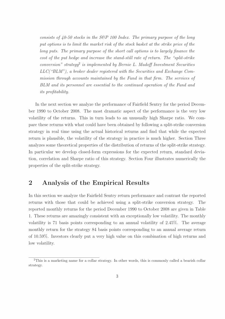
consists of 40-50 stocks in the S&P 100 Index. The primary purpose of the long

put options is to limit the market risk of the stock basket at the strike price of the

long puts. The primary purpose of the short call options is to largely finance the

cost of the put hedge and increase the stand-still rate of return. The “split-strike

conversion” strategy2 is implemented by Bernie L. Madoff Investment Securities

LLC(“BLM”), a broker dealer registered with the Securities and Exchange Com-

mission through accounts maintained by the Fund in that firm. The services of

BLM and its personnel are essential to the continued operation of the Fund and

its profitability.

In the next section we analyze the performance of Fairfield Sentry for the period Decem-

ber 1990 to October 2008. The most dramatic aspect of the performance is the very low

volatility of the returns. This in turn leads to an unusually high Sharpe ratio. We com-

pare these returns with what could have been obtained by following a split-strike conversion

strategy in real time using the actual historical returns and find that while the expected

return is plausible, the volatility of the strategy in practice is much higher. Section Three

analyzes some theoretical properties of the distribution of returns of the split-strike strategy.

In particular we develop closed-form expressions for the expected return, standard devia-

tion, correlation and Sharpe ratio of this strategy. Section Four illustrates numerically the

properties of the split-strike strategy.

2 Analysis of the Empirical Results

In this section we analyze the Fairfield Sentry return performance and contrast the reported

returns with those that could be achieved using a split-strike conversion strategy. The

reported monthly returns for the period December 1990 to October 2008 are given in Table

1. These returns are amazingly consistent with an exceptionally low volatility. The monthly

volatility is 71 basis points corresponding to an annual volatility of 2.45%. The average

monthly return for the strategy 84 basis points corresponding to an annual average return

of 10.59%. Investors clearly put a very high value on this combination of high returns and

low volatility.

2This is a marketing name for a collar strategy. In other words, this is commonly called a bearish collarstrategy.

3

Table 1: Fairfield Sentry monthly returns from Dec. 1990 to Oct. 2008.

Year Jan Feb Mar Apr May Jun Jul Aug Sep Oct Nov Dec

2008 0.63 0.06 0.18 0.93 0.81 -0.06 0.72 0.71 0.50 -0.06 na na2007 0.29 -0.11 1.64 0.98 0.81 0.34 0.17 0.31 0.97 0.46 1.04 0.232006 0.70 0.20 1.31 0.94 0.70 0.51 1.06 0.77 0.68 0.42 0.86 0.862005 0.51 0.37 0.85 0.14 0.63 0.46 0.13 0.16 0.89 1.61 0.75 0.542004 0.88 0.44 -0.01 0.37 0.59 1.21 0.02 1.26 0.46 0.03 0.79 0.242003 -0.35 -0.05 1.85 0.03 0.9 0.93 1.37 0.16 0.86 1.26 -0.14 0.252002 -0.04 0.53 0.39 1.09 2.05 0.19 3.29 -0.13 0.06 0.66 0.09 0.002001 2.14 0.08 1.07 1.26 0.26 0.17 0.38 0.94 0.66 1.22 1.14 0.122000 2.14 0.13 1.77 0.27 1.30 0.73 0.58 1.26 0.18 0.86 0.62 0.361999 1.99 0.11 2.22 0.29 1.45 1.70 0.36 0.87 0.66 1.05 1.54 0.321998 0.85 1.23 1.68 0.36 1.69 1.22 0.76 0.21 0.98 1.86 0.78 0.261997 2.38 0.67 0.80 1.10 0.57 1.28 0.68 0.28 2.32 0.49 1.49 0.361996 1.42 0.66 1.16 0.57 1.34 0.15 1.86 0.20 1.16 1.03 1.51 0.411995 0.85 0.69 0.78 1.62 1.65 0.43 1.02 -0.24 1.63 1.53 0.44 1.031994 2.11 -0.44 1.45 1.75 0.44 0.23 1.71 0.35 0.75 1.81 -0.64 0.601993 -0.09 1.86 1.79 -0.01 1.65 0.79 0.02 1.71 0.28 1.71 0.19 0.391992 0.42 2.72 0.94 2.79 -0.27 1.22 -0.09 0.85 0.33 1.33 1.35 1.361991 3.01 1.40 0.52 1.32 1.82 0.30 1.98 1.00 0.73 2.75 0.01 1.561990 2.77

If these returns were in fact achievable they would dominate those obtained from investing

directly in the S&P 500 Index for instance. In fact investing in the index offers comparable

returns with much higher volatility. Figure 1 compares the Fairfield Sentry (FS) performance

with the strategy of investing directly in the S&P 500 with dividends reinvested over the

period December 1990 to October 2008. It shows how an initial investment of one hundred

would have grown under both assumptions. One hundred invested in the FS fund would

have accumulated to 603.8 by October 2008 whereas one hundred invested in the S&P would

have accumulated to 433.03 by October 2008 reflecting a lower growth rate. The annual

return from investing in the S&P has been 9.64% with a standard deviation of 14.28% over

the 17 years and eleven months period. We note that we assume no expenses in the S&P

investment and it is not clear if the Fairfield Sentry returns are net3 of expenses.

We note that the growth of the investment in Fairfield Sentry is approximately linear.

3It is conventional for hedge fund returns to be quoted net of expenses. These expenses include a fee onthe total assets plus an incentive fee based on the performance of the fund. See Gregoriou and Lhabitant(2009) as well as Markopolos (2009) and SEC (2005) for more discussion on the unusual fee structure ofMadoff’s fund.

4

We also explore this issue in Figure 1. The top green line represents a linear increase of

2.343 per month starting at 100 in December 1990 to October 2008. The bottom green line

assumes that a constant monthly compounded4 growth rate of 84 basis points per year. This

assumes that the fund increases at a constant compound rate of return each month. We note

that the actual performance of the FS Fund lies inside these two green lines.

0 50 100 150 2000

100

200

300

400

500

600

700

800

Time in months: Dec 1990 to Oct 2008

Accu

mul

atio

n

Figure 1: Accumulated investment proceeds using the Fairfield Sentry returns given in Table1 and investment in the S&P 500 with dividends reinvested.

The Fairfield Sentry performance is in red and the S&P 500 accumulation is in blue. The top greenline shows how the initial 100 accumulates to 603.78 in October 2008 if the dollar increase is constantand equal to 2.343 per month. The bottom green line shows how the initial 100 in December 1990accumulates to 603.78 in October 2008 under a constant monthly compounded growth rate.

Given the consistently high returns and the incredibly low volatility of the FS returns it

is of interest to examine what sort of returns could be expected under a split-strike strategy

during this period. To do so, we assume that a hypothetical investor takes a long position in

the S&P 500 Index starting in December 1990. At the same time he buys a put option on the

4 This rate is actually .008398 and it corresponds to a geometric growth rate per month. Thus we have(1.008398)215 = 6.0377.

5

index and sells short a call option on the S&P 500 Index5. For the purpose of illustration,

we assume that the strike price of the put is 5% below the initial spot price of the index and

that the strike price of the call is 5% above the initial spot price of the index6. Both options

are assumed to be European and have a one month maturity. Typically the call price will

exceed the put price and the proceeds are invested for one month at the risk-free rate. At

the end of the month the option positions are settled in cash. If there is a loss under the

option strategy it is financed in the first place from the risk-free investment of the net option

premiums and if that is not enough by selling enough shares of the index.

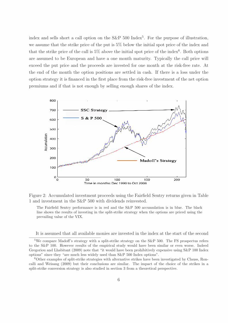
Figure 2: Accumulated investment proceeds using the Fairfield Sentry returns given in Table1 and investment in the S&P 500 with dividends reinvested.

The Fairfield Sentry performance is in red and the S&P 500 accumulation is in blue. The blackline shows the results of investing in the split-strike strategy when the options are priced using theprevailing value of the VIX.

It is assumed that all available monies are invested in the index at the start of the second

5We compare Madoff’s strategy with a split-strike strategy on the S&P 500. The FS prospectus refersto the S&P 100. However results of the empirical study would have been similar or even worse. IndeedGregoriou and Lhabitant (2009) note that “it would have been prohibitively expensive using S&P 100 Indexoptions” since they “are much less widely used than S&P 500 Index options”.

6Other examples of split-strike strategies with alternative strikes have been investigated by Clauss, Ron-calli and Weisang (2009) but their conclusions are similar. The impact of the choice of the strikes in asplit-strike conversion strategy is also studied in section 3 from a theoretical perspective.

6

month and the same option strategy is implemented. This procedure is repeated every month

for 215 months. We ignore transaction costs and any price impact of the trades. In order to

price the options we use the Black-Scholes formula. As a proxy for the implied volatility we

use the VIX to price both7 the call and put options. The average level of the VIX over this

period is 19.24%. We use the prevailing one month US T-bill rates to proxy the risk-free

rates in pricing the options.

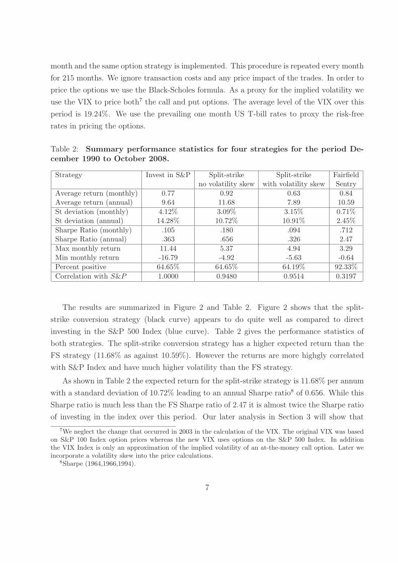
Table 2: Summary performance statistics for four strategies for the period De-

cember 1990 to October 2008.

Strategy Invest in S&P Split-strike Split-strike Fairfieldno volatility skew with volatility skew Sentry

Average return (monthly) 0.77 0.92 0.63 0.84Average return (annual) 9.64 11.68 7.89 10.59

St deviation (monthly) 4.12% 3.09% 3.15% 0.71%St deviation (annual) 14.28% 10.72% 10.91% 2.45%

Sharpe Ratio (monthly) .105 .180 .094 .712Sharpe Ratio (annual) .363 .656 .326 2.47

Max monthly return 11.44 5.37 4.94 3.29Min monthly return -16.79 -4.92 -5.63 -0.64

Percent positive 64.65% 64.65% 64.19% 92.33%

Correlation with S&P 1.0000 0.9480 0.9514 0.3197

The results are summarized in Figure 2 and Table 2. Figure 2 shows that the split-

strike conversion strategy (black curve) appears to do quite well as compared to direct

investing in the S&P 500 Index (blue curve). Table 2 gives the performance statistics of

both strategies. The split-strike conversion strategy has a higher expected return than the

FS strategy (11.68% as against 10.59%). However the returns are more highgly correlated

with S&P Index and have much higher volatility than the FS strategy.

As shown in Table 2 the expected return for the split-strike strategy is 11.68% per annum

with a standard deviation of 10.72% leading to an annual Sharpe ratio8 of 0.656. While this

Sharpe ratio is much less than the FS Sharpe ratio of 2.47 it is almost twice the Sharpe ratio

of investing in the index over this period. Our later analysis in Section 3 will show that

7We neglect the change that occurred in 2003 in the calculation of the VIX. The original VIX was basedon S&P 100 Index option prices whereas the new VIX uses options on the S&P 500 Index. In additionthe VIX Index is only an approximation of the implied volatility of an at-the-money call option. Later weincorporate a volatility skew into the price calculations.

8Sharpe (1964,1966,1994).

7

the split-strike conversion cannot produce a Sharpe ratio twice as big as direct investing in

the index. As we will discuss later, there is a maximum possible Sharpe ratio that could be

achieved (Goetzmann et al. (2002)). So this result is very surprising. Another way could be

to compare the variance and the expected return of Madoff to other stocks and hedge funds.

Clauss et al. (2009) show that all funds that have a significant investment in Madoff’s fund

lie outside the efficiency frontier of the CAPM (see Figure 2 of Clauss et al. (2009)).

The option prices that were used to construct the black curve in Figure 2 or 3 assume

that both the call and put options were priced using the prevailing value of the VIX.

Figure 3: Accumulated investment proceeds using the Fairfield Sentry returns given in Table1 and investment in the S&P 500 with dividends reinvested.

The Fairfield Sentry performance is in red and the S&P 500 accumulation is in blue. The blackline shows the results of investing in the split-strike strategy when the options are priced usingthe prevailing value of the VIX. The green line shows the results of investing in the Split-StrikeConversion strategy when the options are priced using a volatility skew assumption based on datakindly supplied by Prof. Gurdip Bakshi.

It is well known that there is a volatility skew whereby the implied volatility at a fixed

maturity is a decreasing function of the strike price. For example Zhang and Shu (2004) find

that over the five year period from 1995 to 1999 the average implied volatility at the money

for short term options is 19% whereas the average implied volatility for out-of-the money

8

calls is 17% and the average implied volatility for out-of-the money puts is 21%. To obtain

the Figure 3, we use data for the implied volatility skew over 1990 to 2008.

Looking at the impact of the skew complements the study of Clauss et al. (2009). These

authors show that it is possible to construct a split-strike strategy with a very low volatility

but then it also has a very low return (to do so, one needs to buy put options almost at-

the-money). Then, they argue that the only way to obtain a similar trend of the returns

as Madoff’s returns is to assume that Madoff was an outstanding stock-picker. Ignoring the

skew but including an 8.5% extra return per year, Clauss et al. (2009) construct a split-strike

strategy that gives similar returns as Madoff (see Figure 5 of Clauss et al. (2009). Including

the impact of the skew on the strategy’s cost in their study would lead to a much higher

extra return than 8.5%. Note that if Madoff was indeed able to generate an 8.5% additional

return by picking the right stock, then buying so much protection as he claimed would have

been unnecessary.

Manipulation Proof Performance Measures

Recently Goetzmann, Ingersoll, Spiegel and Welch (2007) (GISW) have developed a manip-

ulation free portfolio performance measure. GISW demonstrate that their measure is robust

to various manipulation strategies. Even though their measure was not designed to detect

outright fraud it can provide valuable insights on the nature of the split-strike strategy and

the Fairfield Sentry returns. The formula for the GISW measure Θ for a series of N monthly

returns is defined as follows

Θ =1

(1 − ρ)hln

(1

N

N∑

i=1

[1 + rpi

1 + rfi

]1−ρ)

(1)

where

• rpi is the rate of return on the portfolio for month i ,

• rfi is the risk-free rate for month i ,

• h is the time interval in years. Here h = 112

.

• ρ corresponds to the relative risk aversion of the investor.

GISW note that this measure Θ has an intuitive economic interpretation. It measures the

portfolio’s implied excess return after adjusting for risk. Thus for the risk-free portfolio,

9

Θ = 0. If one had a portfolio that earned exactly fifty basis points above the risk-free rate

every month with no variation this portfolio would have Θ = .06. If the portfolio is risky

then Θ decreases if a more risk-averse investor is considered. Table 3 shows the values of the

GISW measure for direct investment in the S&P, the split-strike strategy (incorporating the

volatility skew) and the Fairfield Sentry returns for different levels of ρ.

Table 3: Values of Θ corresponding to different levels of ρ for three investment

strategies

Value of ρ Invest in S&P Split-strike Fairfieldwith volatility skew Sentry

2 0.0309 0.0237 0.05973 0.0201 0.0177 0.05944 0.0090 0.0117 0.05925 -0.0025 0.0056 0.058910 -0.0664 -0.0254 0.0575

Table 3 shows that the Fairfield Sentry portfolio outperforms the other strategies based

on this measure. If the investor becomes more risk averse the value of Θ declines rapidly for

the investment in the S&P and the split-strike strategy. However Θ hardly changes at all for

the Fairfield Sentry returns. The Fairfield Sentry returns correspond to an extra six percent

per year above the risk-free rate for all investors even the most risk averse. Mr Madoff’s

returns were ingeniously designed to appeal to even the most risk averse investors.

This section showed that returns on Fairfield Sentry portfolio looked very suspicious.

There is empirical evidence that volatility was too low, that the Sharpe ratios were too high

to be true. However they were designed such that any investors would be willing to receive

these returns even the most risk averse. Investors chose to invest with B. Madoff because

they had full confidence in B. Madoff. He was a former chairman of the NASDAQ. “His solid

and consistent track record generated a mixture of amazement, fascination, and curiosity.

Investing with him was an exclusive privilege (...) All Madoff investors should in retrospect

kick themselves for not asking more questions before investing. As many of them have learned

there is no substitute for due diligence (...) there were a number of red flags in Madoff’s

investment advisory business that should have been identified as serious concerns and warded

off potential clients.” (Gregoriou and Lhabitant (2009)). The next section supplements this

empirical study by providing some formal analysis of what the returns under a split-strike

conversion should be in the well-accepted model of Black and Scholes. This theoretical study

10

confirms the previous analysis and shows also that even a simple model could help to identify

a fraud and detect unrealistic returns.

3 Theoretical Analysis of Split-Strike Strategy

The following section is a theoretical analysis of the split-strike strategy. It is implemented in

the standard Black-Scholes framework. The goal of this section is to provide some theoretical

support to the suspicion that Fairfield Sentry portfolio was committing a fraud that could

have been detected much earlier.

The market is assumed to be arbitrage-free. Let S0 be the price of the underlying index

at current time zero. Assume the index pays no dividends and follows a geometric Brownian

motion under the real world measure P so that

dSt = µ St dt + σ St dWt (2)

where Wt is a standard Brownian motion on a probability space (Ω,F , P ) with respect to the

filtration Ft, and µ and σ are constants. The risk-free rate r is constant and continuously

compounded. The index value at time h writes as Sh = S0 exp( (

µ − σ2

2

)h + σWh

). It

follows a lognormal distribution. Its two first moments are given as follows,

EP [Sh] = S0e

µh

VarP [Sh] = S20e

2µh(eσ2h − 1

) (3)

We first describe the split-strike strategy, then derive the first two moments of the standard

call and put options and finally obtain some theoretical results about the expected return,

the standard deviation, the correlation and the Sharpe ratio of the split-strike strategy.

3.1 Split-Strike Strategy

Suppose the time horizon is h. At time zero, the portfolio manager buys one share of the

index and simultaneously sells a call option at a premium c0 and buys a put option at the

premium p0. The call option has a strike price Kc, the put option has a strike price Kp where

Kc > S0 > Kp.

11

Both options have the same time to maturity T ≥ h and are priced by the Black-Scholes

formula. The time zero value of the portfolio V0 is

V0 = S0 = S0 + (c0 − p0) + (long put + short call) (4)

We assume that the amount (c0 − p0) accumulates to the end of the period at the risk-free

rate. The value of the call option (respectively the put option) at time h if the stock price

is Sh is denoted by Ch (respectively Ph). The value of the portfolio at time h is

Vh = Sh + (c0 − p0)erh + (Ph − Ch). (5)

Remark 1 When Kc = Kp = K, the payoff of the strategy is deterministic and equal to

Vh = S0erh (6)

This is a straightforward consequence of the call-put parity. Indeed, the call-put parity

relationship applied at time h implies Vh = Ke−r(T−h) + (c0 − p0)erh. But at time 0, the

call-put parity can be written as c0 − p0 = S0 − Ke−rT . Thus (6) is proved.

We are interested in the general case when Kp the strike of the put option is different

from the strike Kc of the call option. The Sharpe ratio of this portfolio is

SR (Vh) =

EP [Vh]V0

− erh

√VarP [Vh]

V 20

=EP [Vh] − S0e

rh

√VarP [Vh]

(7)

since V0 = S0. The expected value of the portfolio and its standard deviation are respectively

calculated as follows

EP [Vh] = EP [Sh] + EP [Ph] − EP [Ch] + (c0 − p0)e

rh

VarP [Vh] = VarP [Sh] + VarP [Ph] + VarP [Ch] + 2 (CovP (Sh,Ph) − CovP (Sh, Ch) − CovP (Ch,Ph))

To derive expressions of the Sharpe ratio, the expected return and the variance of the

split-strike strategy, we need to know the moments of standard options. The next paragraph

gives the expressions of the first moment of standard options. Second moments are provided

in the appendix.

12

3.2 First moments of standard options under the physical measure

The price dynamics of the underlying asset S under the P measure are given by (2). Denote

by XT the payoff of the option (in the case of the call option XT = max(ST − Kc, 0) and in

the case of the put XT = max(Kp − ST , 0)). Let h be such that 0 < h < T . Denote by Xh

the value of the derivative at time h.

Let us denote by Ch and Ph the value at time h of respectively the call option and the

put option in the Black-Scholes framework. The price is expressed at time h with current

asset price Sh at time h, with respective exercise prices Kc and Kp and maturity T .

Ch := C[Sh, h,Kc, T ], Ph := P [Sh, h,Kp, T ].

Proposition 3.1. First moments of standard options:

The first moments of this call option and this put option are respectively given as follows

EP [Ch] = C[S0e

µh, 0, Kcerh, T

]= S0e

µh Φ(d1(Kc)

)− Kce

rh e−rT Φ(d2(Kc)

), (8)

EP [Ph] = P[S0e

µh, 0, Kperh, T

]= Kpe

rh e−rT Φ(−d2(Kp)

)− S0e

µh Φ(−d1(Kp)

), (9)

where

d1(K) =ln(

S0eµh

Kerh

)+(r + σ2

2

)T

σ√

T; d2(K) = d1(K) − σ

√T

and Φ is the cdf of a standard normal distribution N (0,1).

It turns out that in the case of standard call and put options, explicit formulae for their

first and second moments are available in Cox and Rubinstein (1985)9. A full proof of the

proposition is provided in the appendix.

The first moment of the distribution of the call price has a simple and intuitive form.

Note that the resulting expression is equal to a Black-Scholes call option with the same time

to maturity as the initial call and the same volatility and interest rate. However it has a

higher input asset price and a higher input strike price. The new input asset price is equal

to the expected value (under P ) of the asset price at time h, EP [Sh] = S0eµh. The new

input strike price is equal to the original strike price, respectively Kc or Kp, accumulated at

the risk-free rate.

9Chapter 6, footnote 34 for the first moments and footnote 43 for the covariance between two calls.

13

The limit cases when h = 0 or h = T are easily verified. When h = 0, the result is

well-known. When h = T , the result can be found in the appendix of Goetzmann et al.

(2002,2007).

3.3 Properties of the Split-Strike Strategy

In this section, we present a number of useful results concerning the split-strike conversion

strategy. To derive these results, we use formulae for the moments of the option prices given

in the previous section or in the appendix. The first proposition related to the expected

return under the Split-Strike Conversion strategy.

Proposition 3.2. Expectation of the strategy:

The expected payoff of the strategy is equal to

EP [Vh] = S0eµh − C

[S0e

µh, 0, Kcerh, T

]+ P

[S0e

µh, 0, Kperh, T

]+ (c0 − p0)e

rh.

When Kc = Kp = K, Vh is deterministic and its expectation is equal to EP [Vh] = S0erh.

The result is a consequence of Proposition 3.1. The special case when Kc = Kp = K is

established earlier. See expression (6).

Remark 2 The expected return from the strategy is an increasing function of Kc and an

increasing function of Kp.

Remark 3 The split-strike strategy has a lower expected return and a lower variance than

a direct investment in the index10:

EP [Vh] 6 EP [Sh] and VarP [Vh] 6 VarP [Sh].

Proposition 3.3. Variance and Sharpe ratio of the strategy:

The variance of the strategy at time h is equal to

VarP [Vh] = S20e

2µh(eσ2h − 1

)+ VC + VP − 2CovC,P − 2CovC,S + 2CovS,P

10Proof available from the authors upon request.

14

where

VC = EP [C2h] − EP [Ch]

2

VP = EP [P2h] − EP [Ph]

2

CovC,P = EP [ChPh] − EP [Ch]EP [Ch]

CovC,S = EP [ChSh] − EP [Ch] S0eµh

CovP,S = EP [PhSh] − EP [Ph] S0eµh

First moments can be found in Proposition 3.1 and formulae for second moments are in the

appendix A (see (18) and (19)) and the 3 cross products: EP [ChPh] ,EP [ChSh] ,EP [PhSh]

can be found in the Appendix B.

The Sharpe ratio of the strategy is defined by the equation (7):

SR (Vh) =EP [Vh] − S0e

rh

√VarP [Vh]

where the expectation is given in proposition 3.2.

The Sharpe ratio is not defined when Kp = Kc because both the numerator and the

denominator are equal to zero. This fact will be explained in the numerical analysis in the

following section.

Proposition 3.4. Correlation of the strategy with the index S:

The correlation can be written as

Corr(Vh, Sh) =VarP [Sh] − CovC,S + CovP,S√

VarP [Vh] S0eµh√

eσ2h − 1

where all terms are given in Prop. 3.3.

The correlation of the strategy with the index is of course equal to 0 when Kc = Kp, but

similar to the Sharpe ratio, it is not defined at zero.

4 Numerical Analysis

Consider a split-strike strategy with maturity T = h. Similar results hold when h < T . We

consider two cases. First, we assume the strikes of respectively the call option and the put

option are given by

Kc = S0 + b Kp = S0 − b (10)

15

where b ∈ [0, S0]. Second, we study the case when Kp and Kc are chosen independently. We

will finally discuss optimal choices of the two strikes.

4.1 Case when the strikes are Kc = S0+b, Kp = S0−b with b ∈ [0, S0]

We plot the expected payoff of the strategy and the standard deviation when b varies in

Figure 4. We assume plausible values for the parameters of the financial market. The

conclusions hold for other choices of the volatility σ, the interest rate r, the instantaneous

expected return µ and maturity of the strategy T . Note that it is not necessary that h = T .

0 20 40 60 80 100103

104

105

106

107

108

109

110

111

112

b

Expe

ctatio

n

0 20 40 60 80 1000

5

10

15

20

25

b

Stan

dard

Devia

tion

S0erh

Expected Payoff of the strategy

E[Vh]

Expected payoff of investing in the index:

S0eµ h

Standard deviation of the strategy

std(Vh)

Standard deviation of investing in the index

Figure 4: Expectation and standard deviation of the split-strike strategy.Assume S0 = 100, σ = 20%, µ = 0.1 and r = 0.04. Assume h = 1, T = 1. The strikes of the call andthe put are Kc = S0 + b and Kp = S0 − b. On the left panel, we display the expected payoff of thestrategy and of an investment in the index (EP [V (h)] and EP [Sh]). The right panel represents thestandard deviations std[V (h)] and std[Sh]. The range of b is [0,100].

Consistent with our theoretical findings, Figure 4 shows that the expected return of a

split-strike strategy is always lower than the expected return of investing in the index. A

lower expected return is compensated by a lower standard deviation. Note that as b goes

to 0, the expected payoff of the strategy converges to S0erh which means that the return

of the strategy is the risk-free rate. This is not a surprise because when Kc = Kp = S0,

V (h) = S0erh. In this case V (h) is deterministic and its variance is equal to 0.

Figure 5 displays the Sharpe ratio of the strategy against the Sharpe ratio of investing

in the index with a horizon h = T = 1 year. We observe that the positions in options

can enhance the Sharpe ratio. However the enhancement is bounded from below as well as

16

from above. Goetzmann et al. (2002) show that there is a maximum possible Sharpe ratio

attainable in the complete market of Black-Scholes. The formula for this maximum Sharpe

ratio when h = T is √e

(µ−r)2T

σ2 − 1.

In addition the limit11 of the Sharpe ratio when b → 0,

limb→0+

SR (VT ) =Φ(a2) − Φ(a2)√Φ(a2)(1 − Φ(a2))

where a2 = µ√

T

σ− σ

√T

2, a2 = r

√T

σ− σ

√T

2. When b = 0, the strategy is equivalent to investing

in bonds and the Sharpe ratio is not defined.

0 10 20 30 40 50 60 70 80 90 1000.24

0.25

0.26

0.27

0.28

0.29

0.3

0.31

Sh

arp

e R

atio

b

Sharpe Ratio of the Split−Strike Strategy

Sharpe Ratio of Investingin the Index

Maximum Sharpe Ratio

Figure 5: Sharpe ratio of the split-strike conversion strategy compared to the Sharpe ratioof investing in the index.

Here σ = 20%, µ = 0.1, r = 0.04 and h = 1, T = 1. The strikes of the call and the put arerespectively equal to Kc = S0 + b and Kp = S0 − b, b ∈ [0, 100].

Figure 5 assumes σ = 20%, µ = 0.1, r = 0.04 and h = T = 1 year. In this case, the

minimum Sharpe ratio is 0.2432 and the maximum Sharpe ratio is equal to 0.3069. Note

also that Figure 5 is consistent with Figure 3 of Lhabitant (1998).

11Proof available from the authors upon request.

17

Finally, in Figure 6 we investigate the correlation between the strategy and the index

and the beta of the strategy. We assume the underlying index S is a good proxy for the

financial market. Then the beta is defined as follows:

β =CovP

(Vh

V0, Sh

S0

)

VarP

(Sh

S0

) =CovP (Vh, Sh)

VarP (Sh)

Formulas for the covariance of Vh and Sh are established in Proposition 3.3 and explicitly

given in the Appendix B.

0 50 1000.7

0.75

0.8

0.85

0.9

0.95

1

b

Corre

lation

betwe

en V

and S

0 50 1000

0.1

0.2

0.3

0.4

0.5

0.6

0.7

0.8

0.9

1

b

Beta

β of th

e stra

tegy

Figure 6: Correlation between Sh and Vh and Beta of the strategy.Here σ = 20%, µ = 0.1, r = 0.04 and h = T = 1. The strikes of the call and the put are respectivelyequal to Kc = S0 + b and Kp = S0 − b. b ∈ [0, 100].

Figure 6 shows that the strategy is highly correlated with the index and that the beta

lies between zero and one. When b = 0, the strategy is deterministic and the correlation is

not defined but the beta is defined and equal to 0. Similar to the Sharpe ratio, the limit of

the correlation when b → 0+ is positive

limb→0+

Corr (VT , ST ) =Φ(a1) − Φ(a2)√

Φ(a2)(1 − Φ(a2)) (eσ2T − 1)

where12 a1 = µ√

T

σ+ σ

√T

2, a2 = µ

√T

σ− σ

√T

2. If b > 0, the correlation is always greater

12Proof available from the authors upon request.

18

than 0.732 (which is its limit calculated with the same parameters as before). However, as

reported to the SEC in 2005 by H. Markopolos, the beta of the strategy was 0.06 and the

correlation with the index was only 0.3 (see attachment 1 on Fairfield Sentry Performance

Data in 2005 in SEC(2005)). The formal analysis in this section confirms that the returns

claimed by Madoff are theoretically impossible.

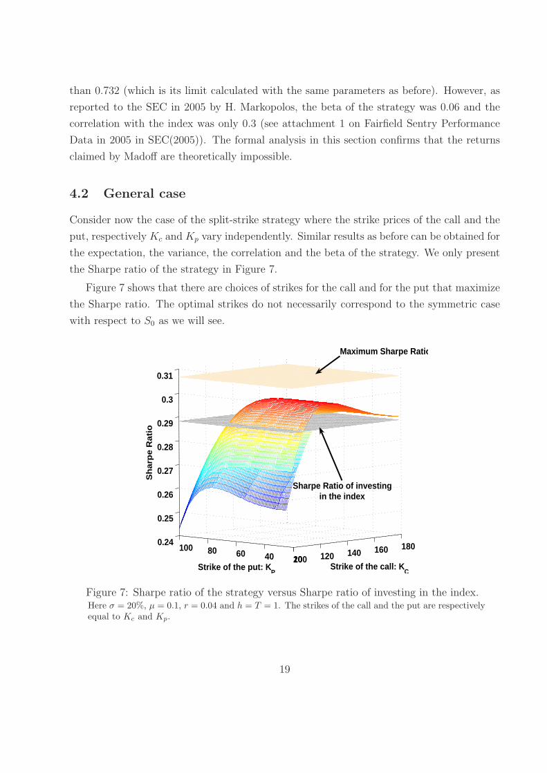
4.2 General case

Consider now the case of the split-strike strategy where the strike prices of the call and the

put, respectively Kc and Kp vary independently. Similar results as before can be obtained for

the expectation, the variance, the correlation and the beta of the strategy. We only present

the Sharpe ratio of the strategy in Figure 7.

Figure 7 shows that there are choices of strikes for the call and for the put that maximize

the Sharpe ratio. The optimal strikes do not necessarily correspond to the symmetric case

with respect to S0 as we will see.

100 120 140 160 18020406080100

0.24

0.25

0.26

0.27

0.28

0.29

0.3

0.31

Strike of the call: KCStrike of the put: K

P

Sh

arp

e R

atio

Maximum Sharpe Ratio

Sharpe Ratio of investingin the index

Figure 7: Sharpe ratio of the strategy versus Sharpe ratio of investing in the index.Here σ = 20%, µ = 0.1, r = 0.04 and h = T = 1. The strikes of the call and the put are respectivelyequal to Kc and Kp.

19

4.3 Optimal choice of the parameters Kp and Kc

In this last subsection, we numerically derive the optimal strikes of the put and of the call in

a split-strike strategy for different choices of the horizon h = T . The objective is to maximize

the Sharpe ratio over the given maturity.

Figure 8: Choice of the strikes Kc and Kp to maximize the Sharpe ratioHere σ = 20%, µ = 10% and r = 4%. The strikes of the call and the put are respectively equal to Kc

and Kp. On the left panel, the optimal strikes K∗c and K∗

p are determined in the general case. Onthe right panel, the optima are compared with the ones obtained by maximizing the Sharpe ratiowhen strikes are symmetric with respect to S0. In this case, the optima are denoted by Kc = S0 +b∗

and Kp = S0 − b∗

0 0.5 1 1.5 2 2.5 30

20

40

60

80

100

120

140

Maturity h

Str

ike

s

Kc* : Optimal Call strike

maximizing the Sharpe ratio of the Split−Strike strategy with horizon h

Kp* : Optimal Put strike

maximizing the Sharpe ratio of the Split−Strike strategy with horizon h

0 0.5 1 1.5 2 2.5 30

20

40

60

80

100

120

140

160

Maturity h

Str

ike

s

Kp*

S0 − b*

S0 + b*

Kc*

As mentioned in the literature by Goetzmann et al. (2007) and by Cvitanic, Lazrak and

Wang (2009), the choice of the horizon can dramatically change the results. With a longer

horizon, it is optimal to buy a call with a higher strike and a put with a lower strike. Note

also that it is optimal not to have a perfectly symmetric split-strike strategy. It is optimal

to buy a put option more deeply out-of-the-money than the call option.

20

5 Conclusions

This paper analyzed certain features of Bernie Madoff’s investment performance. It is now

known that these results were based on a giant Ponzi scheme which flourished for a long

time despite several red flags and the highly suspicious nature of the returns. Indeed were it

not for the current financial crisis it seems likely that the Madoff investment scheme would

still be in operation.

We implemented a version of the split-strike strategy similar to the one allegedly used

by Madoff and compared the results with those reported by Fairfield Sentry one of Madoff’s

feeder funds. The Sharpe ratio based on our version of the split strike strategy was very much

lower than Fairfield Sentry’s Sharpe ratio over the same period. In addition the correlation

between the split-strike strategy and the market was more than twice the corresponding

correlation for the Madoff strategy. One of the most unbelievable statistics of Madoff’s

performance is the very low volatility. This makes the Madoff’s returns very attractive even

to the most risk averse investors. These returns were concocted in a very clever way.

Our theoretical analysis reaches the same conclusions. There are closed-form expressions

for the moments of the split strike strategy and its correlation with the market. In addition

there is a theoretical maximum Sharpe ratio that can be obtained using options. We find

that the performance statistics reported by Fairfield Sentry lie well outside their theoretical

bounds. These results are incredible in the most literal sense.

In summary there are some simple quantitative diagnostics that should have raised sus-

picions about Madoff’s performance.

21

Appendix

Let us first recall some of the key properties of the normal distribution and of the bivariatenormal distribution that will be useful to derive a closed-form expression of the Sharperatio of the strategy under study. Consider X ∼ N (µx, σ

2x) and denote by g (x, µx, σ

2x) the

corresponding pdf. Let c ∈ R. The pdf of X satisfies

g(x, µx, σ

2x

)ecx = g(x, µx + cσ2

x, σ2x) eµxc+

c2σ2x

2 , (11)

or in other words, if fX denotes the pdf of X then

fX (x) ecx = fX+cσ2x(x) eµxc+

c2σ2x

2 .

Consider (X,Y ) following the bivariate distribution

(X,Y ) ∼ N2

(µx, σ

2x, µy, σ

2y , ρ),

then X ∼ N (µx, σ2x) and Y ∼ N

(µy, σ

2y

)are two correlated normal random variables with

correlation coefficient ρ. The pdf of (X,Y ) can be written as

f(x, µx, σ

2x, y, µy, σ

2y , ρ)

=1

2π

1

σxσy (1 − ρ2)e−(

(x−µx )2

σ2x

+(y−µy )2

σ2y

−2ρ(x−µx )(y−µy )

σxσy

)

.

We are going to make use of one particular property of the pdf of the bivariate normaldistribution. Given two real numbers α, β, one has

eαx+βy f(x, 0, σ2

x, y, 0, σ2y , 0)

= eα2

2+β2

2 f(x, ασ2

x, σ2x, y, βσ2

y , σ2y , 0). (12)

We will have to correctly choose α and β to calculate the different integrals that will appearlater in our calculations.

A Moments of Standard Options

Using standard results, the price at time h of an option can be expressed as a conditionalexpectation under the risk neutral measure Q defined by its Radon-Nikodym derivative:

LT :=dQ

dP= exp

−(

µ − r

σ

)WT − 1

2

(µ − r)2

σ2T

. (13)

Then from the Girsanov theorem, we know that under the new probability measure Q,Bt = Wt + µ−r

σt is a standard Brownian motion with respect to Ft and the stock price

dynamic are expressed as dSt = r St dt + σ St dBt.

22

The price of the derivative at time h can be expressed as

Xh = e−r(T−h)EQ [XT |Fh] . (14)

We are interested in EP [Xh], the expectation under the physical measure of the value attime h of the strategy. Using equation (14) we can derive a compact expression for the firstmoment of the distribution as a double expectation with the outer expectation taken overthe P -measure and the inner expectation over the Q-measure.

First moment of the call option

The expression we want to calculate is given by

EP [Ch] = EP

[e−r(T−h)

EQ

[max (ST − K)+ | Fh

]].

Using Black-Scholes formula, one obtains,

EP [Ch] = EP

[ShΦ (d1) − Ke−r(T−h) Φ (d2)

],

where

d1 =ln(

Sh

K

)+(r + σ2

2

)(T − h)

σ√

T − h, d2 = d1 − σ

√T − h.

Since Wt is a standard Brownian motion under P , WT−Wh√T−h

is independent of Fh and followsa standard normal distribution, one can also write the above formula as follows:

EP [Ch] = EP

[ShEP

[1WT −Wh

√

T−h<d1

| Fh

]]− Ke−r(T−h)

EP

[EP

[1WT −Wh

√

T−h<d2

| Fh

]]. (15)

However, as we have that Sh = S0eµh−σ2

2h+σWh , we get

d1 = Wh√T−h

+ln(S0

K )+(µ−σ2

2

)h+(r+σ2

2

)(T−h)

σ√

T−h= Wh√

T−h+ d,

d2 = Wh√T−h

+ d − σ√

T − h,

where

d =ln(

S0

K

)+(µ − σ2

2

)h +

(r + σ2

2

)(T − h)

σ√

T − h.

The calculation of (15) can be split into two parts:

23

• The second part is straightforward:

EP

[EP

[1WT −Wh

√

T−h<d2

| Fh

]]= P

(WT − Wh√

T − h− Wh√

T − h< d − σ

√T − h

)

= Φ

((d − σ

√T − h)

√T − h

T

).

The last equality comes from the fact that WT−Wh√T−h

− Wh√T−h

∼ N(0,√

TT−h

).

• For the first part, we can write it as

S0e

(µ−σ2

2

)hEP

[e

σ√

T−hWh

√

T−hEP

[1WT −Wh

√

T−h<d1

| Fh

]](16)

WT−Wh√T−h

and Wh√T−h

are two independent normally distributed random variables. Thus

the expectation term in (16) can be also written as the following double integral

∫ +∞

−∞

∫ +∞

−∞eσ

√T−hx

1y+x<d f

(x, 0,

h

T − h, y, 0, 1, 0

)dxdy.

Applying formula (12) with α = σ√

T − h and β = 0, one obtains

eσ2(T−h)

2

∫ +∞

−∞

∫ +∞

−∞1y+x<d f

(x, σ

h√T − h

,h

T − h, y, 0, 1, 0

)dxdy,

which is equal to the probability a normally distributed X ∼ N(σ h√

T−h, T

T−h

)is less

than d:

eσ2(T−h)

2 Φ

d − σ h√

T−h√T

T−h

.

Then one obtains the following (simple) expression:

EP [Ch] = S0eµhΦ

(log(

S0

K

)+ ε1

σ√

T

)− Ke−r(T−h)Φ

(log(

S0

K

)+ ε2

σ√

T

)

where ε1 =(µ + σ2

2

)T − (µ − r) (T − h) and ε2 = ε1 − σ2T . We recognize the expression of

the price of a call option:

EP [Ch] = S0eµhΦ

(d1

)− (Kerh)e−rT Φ

(d2

)= C

[S0e

µh, 0, Kerh, T],

24

where

d1 =log(

S0eµh

Kerh

)+(r + σ2

2

)T

σ√

Td2 = d1 − σ

√T . (17)

The proof of the first moment of the put option is similar and omitted.

Second moment of the call option

Proposition A.1. Second moments of standard options:The second moments of the call and put option are given as follows,

EP

[C2

h

]= S2

0e2µheσ2hΦ2

(d1(Kc) +

σh√T

, d1(Kc) +σh√T

,h

T

)

−2Ke−r(T−h)S0eµhΦ2

(d1(Kc), d2(Kc) +

σh√T

,h

T

)

+K2e−2r(T−h)Φ2

(d2(Kc), d2(Kc),

h

T

)(18)

EP

[P2

h

]= S2

0e2µheσ2hΦ2

(−d1(Kp) −

σh√T

, −d1(Kp) −σh√T

,h

T

)

−2Ke−r(T−h)S0eµhΦ2

(−d1(Kp), −d2(Kp) −

σh√T

,h

T

)

+K2e−2r(T−h)Φ2

(−d2(Kp), −d2(Kp),

h

T

)(19)

where

d1(K) =ln(

S0eµh

Kerh

)+(r + σ2

2

)T

σ√

T; d2(K) = d1(K) − σ

√T

and where Φ2(x, y, ρ) is the bivariate standard normal distribution function with correlationparameter ρ.

Remark 4 In the case when h = T , the result is given in the appendix of Goetzmann etal. (2007). In this case, the result can be simplified and expressed as a combination of theunivariate standard normal distribution (since Φ2(a, b, 1) = Φ(min(a, b))).

The Black-Scholes call price expressed at time h with current asset price Sh at time h,with exercise price K and with maturity T is given by

Ch = Sh Φ(d1) − K e−r(T−h)Φ(d2)

25

where

d1 =ln(

Sh

K

)+(r + σ2

2

)(T − h)

σ√

T − h, d2 = d1 − σ

√T − h.

We are now looking for an expression of the second moment:

EP

[C2

h

]= EP

[S2

hΦ(d1)2 − 2ShΦ(d1)Ke−r(T−h)Φ(d2) + K2e−2r(T−h)Φ(d2)

2]

= E1 − 2Ke−r(T−h)E2 + K2e−2r(T−h)E3.

Let us get an expression for the 3 expectations that appear in the above sum:

E1 := EP

[S2

hΦ(d1)2], E2 := EP [ShΦ(d1)Φ(d2)] , E3 := EP

[Φ(d2)

2]

Computation of the first term E1:

E1 = S20e

2µh−σ2hEP

e2σX Φ

σX + ln

(S0e

(µ−

σ2

2

)h

K

)+(r + σ2

2

)(T − h)

σ√

T − h

2

where X = Wh is independent of the σ-field Ft and follows N (0, h). Let us define by Y andZ random variables independent of X and of the σ-field Ft that both follow N (0, T − h).Denote by

k :=1

σln

S0e

(µ−σ2

2

)h

K

+

(r +

σ2

2

)(T − h)

σ.

Therefore,E1 = S2

0e2µh−σ2h

EP

[e2σX P (Y < X + k) P (Z < X + k)

].

This could be written in terms of integrals

E1 = S20e

2µh−σ2h

∫ +∞

−∞

∫ +∞

−∞

∫ +∞

−∞e2σx

1y−x<k1z−x<kg(x, 0, h)g(y, 0, T )g(z, 0, T )dxdydz,

where g(x, µx, σ2x) denotes the pdf of N (µx, σ

2x). Using (11), it could be rewritten as

E1 = S20e

2µh+σ2h

∫ +∞

−∞

∫ +∞

−∞

∫ +∞

−∞1y−x<k1z−x<kg(x, 2σh, h)g(y, 0, T )g(z, 0, T )dxdydz.

Denote by X = X + 2σh. The above expression could now be written as

E1 = S20e

2(µ−σ2

2

)hP(Y − X < k, Z − X < k

),

26

where (Y − X, Z − X) follows a bivariate normal distribution. Y − X ∼ N (−2σh, T ),

Z − X ∼ N (−2σh, T ) and the correlation is ρ = hT. Thus,

E1 = S20e

2µheσ2hΦ2

(γ, γ,

h

T

),

where

γ :=

ln

(S0e

(µ−

σ2

2

)h

K

)+(r + σ2

2

)(T − h) + 2σ2h

σ√

T

and Φ2(a, b, ρ) is the probability that X < a and Y < b when (X,Y ) are two standardN (0, 1) r.v. following a bivariate normal distribution with correlation ρ. The expressioncould be simplified as follows:

E1 = S20e

2µheσ2hΦ2

(d1 +

σh√T

, d1 +σh√T

,h

T

)

where d1 is defined earlier (see expression (17)).

Computation of the second term E2 := EP [ShΦ(d1)Φ(d2)] .

One can also write it as

E2 = S0e

(µ−σ2

2

)hEP

[eσX Φ

(X + k√T − h

)Φ

(X + p√T − h

)|Ft

],

where X = Wh is Fh-measurable follows N (0, h) and where k and p are given by

k := 1σ

ln

(S0e

(µ−

σ2

2

)h

K

)+(r + σ2

2

)(T−h)

σ,

p := 1σ

ln

(S0e

(µ−

σ2

2

)h

K

)+(r − σ2

2

)(T−h)

σ.

Note that p and k are both Fh measurable. Let us now define by Y and Z two randomvariables independent of X and of the σ-field Fh that both follow N (0, T − h). E2 could bewritten in terms of integrals,

E2 = S0eµh−σ2

2h

∫ +∞

−∞

∫ +∞

−∞

∫ +∞

−∞eσx

1y−x<k1z−x<pg(x, 0, h)g(y, 0, T )g(z, 0, T )dxdydz,

27

where g(x, µx, σ2x) denotes the pdf of N (µx, σ

2x). Using (11), it could be rewritten as:

E2 = S0eµh

∫ +∞

−∞

∫ +∞

−∞

∫ +∞

−∞1y−x<k1z−x<pg(x, σh, h)g(y, 0, T )g(z, 0, T )dxdydz.

Denote by X = X + σh. The above expression could now be written as:

E2 = S20e

µhP(Y − X < k, Z − X < p

),

where (Y − X, Z − X) follows a bivariate normal distribution. Y − X ∼ N (−σh, T ),

Z − X ∼ N (−σh, T ) and the correlation is ρ = hT. Thus, E2 = S0e

µhΦ2

(k+σh√

T, p+σh√

T, h

T

).

The expression could be simplified as

E2 = S0eµhΦ2

(d1, d2 +

σh√T

,h

T

)

where d2 was defined earlier by (17).

Computation of the third term E3: Similarly, one obtains

E3 = Φ2

(d2, d2,

h

T

).

Second moment of the Put Option

Similarly, one can prove that

EP

[P2

h

]= F1 − 2Ke−r(T−h)F2 + K2e−2r(T−h)F3

where the 3 expectations Fi are defined as follows:

F1 := EP

[S2

hΦ(−d1)2], F2 := EP [ShΦ(−d1)Φ(−d2)] , F3 := EP

[Φ(−d2)

2]

Omitting the details, one obtains

F1 = S20e

2µheσ2hΦ2

(−d1 − σh√

T, −d1 − σh√

T, h

T

)

F2 = S0eµhΦ2

(−d1, −d2 − σh√

T, h

T

)

F3 = Φ2

(−d2, −d2,

hT

).

28

B Computation of the Covariance terms

Ch = Sh Φ(d1(Kc)) − Kc e−r(T−h)Φ(d2(Kc))

Ph = Kp e−r(T−h)Φ(−d2(Kp)) − Sh Φ(−d1(Kp))

where d1(K) =ln(

ShK

)+(r+σ2

2

)(T−h)

σ√

T−h, d2(K) = d1(K) − σ

√T − h.

EP [ChPh] = Kpe−r(T−h)EP [ShΦ (d1(Kc)) Φ (−d2(Kp))]

−KcKpe−2r(T−h)EP [Φ (d2(Kc)) Φ (−d2(Kp))]

−EP [S2hΦ (d1(Kc)) Φ (−d1(Kp))]

+Kce−r(T−h)EP [ShΦ (d2(Kc)) Φ (−d1(Kp))]

EP [ChSh] = EP [S2h Φ (d1(Kc))] − Kc e−r(T−h)EP [ShΦ (d2(Kc))]

EP [PhSh] = Kp e−r(T−h)EP [ShΦ (−d2(Kp))] − EP [S2h Φ (−d1(Kp))]

The formulas for these expectations are given as follows,

EP [ShΦ(d1)Φ(−d2)] = S0eµhΦ2

(d1(Kc), −d2(Kp) −

σh√T

, − h

T

)

EP [Φ(d2)Φ(−d2)] = Φ2

(d2(Kc),−d2(Kp), − h

T

)

EP

[S2

hΦ(d1)Φ(−d1)]

= S20e

2µheσ2hΦ2

(d1(Kc) +

σh√T

, −d1(Kp) −σh√T

, − h

T

)

EP [ShΦ(−d1)Φ(d2)] = S0eµhΦ2

(−d1(Kp), d2(Kc) +

σh√T

,−h

T

)

EP

[S2

h Φ(d1)]

= S20e

2µheσ2hΦ

(d1(Kc) +

σh√T

)

EP [ShΦ(d2)] = S0eµhΦ

(d2(Kc) +

σh√T

)

EP [ShΦ(−d2)] = S0eµhΦ

(−d2(Kp) −

σh√T

)

EP

[S2

h Φ(−d1)]

= S20e

2µheσ2hΦ

(−d1(Kp) −

σh√T

)

where

d1(K) =ln(

S0eµh

Kerh

)+ (r + σ2

2)T

σ√

T, d2(K) = d1 − σ

√T

29

References

[1] Bhattacharya U. (2003) “The optimal design of Ponzi schemes in finite economies”,Journal of Financial Intermediation, 12(1), 2-24.

[2] Clauss P., T. Roncalli and G. Weisang (2009) “Risk Management Lessons from MadoffFraud”, Working Paper available at http://ssrn.com/abstract=1358086.

[3] Credit Suisse report (14 January 2009) Market Commentary, Equity Derivatives Strat-egy, “Split-Strike Conversions” by E. Tom and S. Palsson.

[4] Cox J.C. and M. Rubinstein (1985) “Options Markets”, Prentice Hall, 1985.

[5] Cvitanic J., A. Lazrak and T. Wang (2009) “Implications of the Sharpe Ratio as aPerformance Measure in Multi-Period Settings”, Journal of Economic Dynamics andControl, 32, 1622-1649.

[6] Goetzmann W., J. Ingersoll, M. Spiegel and I. Welch (2002) “Sharpening Sharpe Ratios”NBER Working Paper Series, Paper No 9116.

[7] Goetzmann W., J. Ingersoll, M. Spiegel and I. Welch (2007) “Portfolio Performance Ma-nipulation and Manipulation-proof Performance Measures”, Review of Financial Stud-ies, 20(5), 1503-1546.

[8] Gregoriou G. and F.-S. Lhabitant (2009) “Madoff: A Riot of Red Flags”, WorkingPaper, EDHEC Risk and Asset Management Research Center.

[9] Hull J.C. (2008) “Options, Futures, and Other Derivatives”, Prentice Hall, 7th edition.

[10] Lhabitant F.-S. (1998) “Derivatives in portfolio management Why beating the marketis easy”, Working Paper, EDHEC Risk and Asset Management Research Center.

[11] Markopolos H. (2009) “Testimony to the US House of Representatives”, Committee onFinancial Services, February 4.

[12] SEC (2005) “The World’s Largest Hedge Fund is a Fraud”, Report submitted to theSEC, November 7, 2005.

[13] Sharpe W. (1964) “Capital Asset Prices: A Theory of Market Equilibrium under con-dition of Risk”, Journal of Finance, 19, 425-442.

[14] Sharpe W. (1966) “Mutual Fund Performance”, Journal of Business, 39, 119-138.

[15] Sharpe W. (1994) “The Sharpe Ratio”, Journal of Portfolio Management, 49-58.

[16] Zhang J.E. and J. Shu (2003) “Pricing S&P 500 Index Options with Heston’s Model”,2003 IEEE International Conference on Computational Intelligence for Financial Engi-neering.

30